Symmetry, Integrability and Geometry: Methods and Applications SIGMA 15 (2019), 018, 20 pages

Perspectives on the Asymptotic Geometry

of the Hitchin Moduli Space

Laura FREDRICKSON

Stanford University, Department of Mathematics, 380 Serra Mall, Stanford, CA 94305, USA

E-mail: lfredrickson@stanford.edu

URL: https://web.stanford.edu/~ljfred4/

Received September 23, 2018, in final form February 25, 2019; Published online March 11, 2019

https://doi.org/10.3842/SIGMA.2019.018

Abstract. We survey some recent developments in the asymptotic geometry of the Hitchinmoduli space, starting with an introduction to the Hitchin moduli space and hyperkahlergeometry.

Key words: Hitchin moduli space; Higgs bundles; hyperkahler metric

2010 Mathematics Subject Classification: 53C07; 53C26

Fix a compact Riemann surface C. In his seminal paper “The self-duality equations ona Riemann surface” [22], Hitchin introduced the moduli spaceM of SL(2,C)-Higgs bundles on Cand proved that M admits a hyperkahler metric gM. In these notes, we give an introductionto the hyperkahler geometry of the Hitchin moduli space, focusing on the geometry of the endsof the Hitchin moduli space. In the last section (Section 4), we briefly survey some recentdevelopments in the description of the asymptotic geometry of M. We start with Gaiotto–Moore–Neitzke’s conjectural description in [17, 18] and survey recent progress in [12, 13, 14,27, 28]. We take a meandering path through more classical geometric results to get there. InSection 1, we give a survey of the results in Hitchin’s original paper [22], since many currentlines of research originate there. In Section 2, we focus on the hyperkahler metric on theHitchin moduli space. In order to more fully describe the conjectured picture of the hyperkahlermetric on the Hitchin moduli space, we take a detour into the classification of noncompacthyperkahler 4-manifolds as ALE, ALF, ALG, and ALH, highlighting some classical and morerecent results. In Section 3, we consider the spectral data of the Hitchin moduli space. Wedescribe the abelianization of Hitchin’s equations near the ends of the moduli space, and theresulting importance of the spectral data for the asymptotic geometry.

1 A tour of the Hitchin moduli space

Given the data of

• C, a compact Riemann surface of genus γC ≥ 2 (unless indicated otherwise), and

• E → C, a complex vector bundle of rank n

we get a Hitchin moduli space M.

In one avatar, the Hitchin moduli space is the moduli space of GL(n,C)-Higgs bundles upto equivalence. In another avatar, the Hitchin moduli space is the moduli space of GL(n,C)-flat connections up to equivalence. In this section, we define these objects and explain thecorrespondence between Higgs bundles (a holomorphic object) and flat connections and their

This paper is a contribution to the Special Issue on Geometry and Physics of Hitchin Systems. The fullcollection is available at https://www.emis.de/journals/SIGMA/hitchin-systems.html

arX

iv:1

809.

0573

5v2

[m

ath.

AG

] 1

1 M

ar 2

019

2 L. Fredrickson

associated representations (a representation theoretic object). We survey many of the resultsappearing in Nigel Hitchin’s seminal paper for the complex Lie group GC = SL(2,C) [22].

1.1 Motivation: Narasimhan–Seshadri correspondence

For the sake of motivation, there is an earlier example of a correspondence between holomorphicobjects and representations. In 1965, Narasimhan and Seshadri proved the equivalence betweenstable holomorphic vector bundles on a compact Riemann surface C and irreducible projectiveunitary representations of the fundamental group [31]. In 1983, Donaldson gave a more directproof of this fact using the differential geometry of connections on holomorphic bundles [10].We specialize to the degree 0 case for simplicity, so that projective unitary representations aresimply unitary representations.

Theorem 1.1 ([10]). Let E be a indecomposable holomorphic bundle of deg E = 0 and rankn over a Riemann surface C. The holomorphic bundle E is stable if, and only if, there is anirreducible flat unitary connection on E. Taking the holonomy representation of this connection,we have the following equivalence:

stable holomorphic bundlesE

/∼↔

flat U(n)-connections∇

/∼

↔

irreducible representationsρ : π1(C)→ U(n)

/∼

.

This map from a holomorphic bundle E to a flat connection ∇ features a distinguishedhermitian metric h on E . First, note that given any hermitian metric h on a holomorphicbundle E , there is a unique connection D(∂E , h) called the Chern connection characterized bythe property that (1) D0,1 = ∂E and (2) D is unitary with the respect to h, i.e., d〈s1, s2〉h =〈Ds1, s2〉h + 〈s1, Ds2〉h. The proof of Theorem 1.1 relies on the following fact: given a stableholomorphic bundle E of degree 0, there is a hermitian metric h – known as a Hermitian–Einsteinmetric – such that the Chern connection is flat. Consequently, the flat connection associatedto E is ∇ = D(∂E , h), where h is the Hermitian–Einstein metric.

The nonabelian Hodge correspondence, which interpolates between the two avatars of theHitchin moduli space, also features a distinguished hermitian metric.

1.2 Definition of the Hitchin moduli space

Higgs bundles and the Hitchin moduli space first appeared in Nigel Hitchin’s beautiful paper“The self-duality equations on a Riemann surface” [22]. We specialize to the degree 0 case forsimplicity.

Definition 1.2. Fix a complex vector bundle E → C of degree 0. A Higgs bundle on E → Cis a pair (∂E , ϕ) where

• ∂E is a holomorphic structure on E (We’ll denote the corresponding holomorphic vectorbundle by E = (E, ∂E).)

• ϕ ∈ Ω1,0(C,EndE) is called the “Higgs field”

satisfying ∂Eϕ = 0. (Alternatively, the Higgs field is a holomorphic map ϕ : E → E ⊗KC , whereKC = T 1,0(C) is the canonical bundle.)

Remark 1.3. If we want GC = SL(n,C) rather than GL(n,C), we must impose the conditiontrϕ = 0, since sl(n,C) consists of traceless matrices. Additionally, we insist that Det E ' OC ,as holomorphic line bundles.

Perspectives on the Asymptotic Geometry of the Hitchin Moduli Space 3

Definition 1.4. Fix a Higgs bundle (E , ϕ). A hermitian metric on E, the underlying complexvector bundle, is harmonic if

FD(∂E ,h) +[ϕ,ϕ∗h

]= 0.

Here FD is the curvature of D; ϕ∗h is the hermitian adjoint1 of ϕ with respect to h.

Definition 1.5. A triple (∂E , ϕ, h) is a solution of Hitchin’s equations if (∂E , ϕ) is a Higgsbundle and h is harmonic, i.e.,

∂Eϕ = 0, FD(∂E ,h) +[ϕ,ϕ∗h

]= 0. (1.1)

Definition 1.6. Fix a complex vector bundle E → C. The associated Hitchin moduli space Mconsists of triples

(∂E , ϕ, h

)solving Hitchin’s equations, up to complex gauge equivalence

g · (∂E , ϕ, h) =(g−1 ∂E g, g−1ϕg, g · h

), where (g · h)(v, w) = h(gv, gw),

for g ∈ Γ(C,Aut(E)).

The Hitchin moduli space is a manifold with singularities. When γC ≥ 2, the dimension ofthe U(n)-Hitchin moduli space is dimRM(C,U(n)) = 4

(n2(g − 1) + 1

); the dimension of the

SU(n)-Hitchin moduli space is dimRM(C,SU(n)) = 4(n2 − 1

)(g − 1).

Exercise 1.7. Verify that the following triple (∂E , tϕ, ht) on C solves Hitchin’s equations:

∂E = ∂, tϕ = t

(0 1z 0

)dz, ht =

(|z|1/2eut(|z|)

|z|−1/2e−ut(|z|)

),

where ut = ut(|z|) is the solution of the ODE(d2

d|z|2+

1

|z|d

d|z|

)ut = 8t2|z| sinh(2ut),

with boundary conditions ut(|z|) ∼ −12 log |z| near |z| = 0 and lim

|z|→∞ut(|z|) = 0. It may be

useful to note:

• In a local holomorphic frame where ∂E = ∂, the curvature is FD(∂E ,h) = ∂(h−1∂h

).

When h is diagonal, FD(∂E ,h) = ∂∂ log h.

• Let z = x+ iy be a local holomorphic coordinate. Then, ∂∂ν = 14

(d2

dx2+ d2

dy2

)ν dz ∧ dz.

Note: This is the model solution featured in [14, 18, 27]. The base curve is CP1 with anirregular singularity at ∞ [15].

1.3 Nonabelian Hodge correspondence

The Hitchin moduli space M is hyperkahler. As a consequence, it has a CP1-worth of complexstructures, labeled by parameter ζ ∈ CP1. Two avatars of the Hitchin moduli space are

• the Higgs bundle moduli space (ζ = 0), and

• the moduli space of flat GL(n,C)-connections ζ ∈ C×.

1In a local holomorphic coordinate z and a local holomorphic frame for (E, ∂E), if ϕ = Φdz, then ϕ∗h =h−1Φ∗hdz.

4 L. Fredrickson

Starting with the triple [(∂E , ϕ, h)] in M, the associated Higgs bundle[(∂E , ϕ

)]is obtained

by forgetting the harmonic metric h. Starting with the triple[(∂E , ϕ, h

)], for each ζ ∈ C×, the

associated flat connection is [∇ζ ] where

∇ζ = ζϕ+D(∂E ,h) + ζ−1ϕ∗h . (1.2)

The nonabelian Hodge correspondence describes the correspondence between solutions of Hit-chin’s equations, Higgs bundles, and flat connections. It answers questions that include “WhatHiggs bundles admit harmonic metrics?” and “Can any flat connection be produced in thisway?”

Exercise 1.8. Use Hitchin’s equations in (1.1) to verify that ∇ζ in (1.2) is flat.

What Higgs bundles (E , ϕ) admit harmonic metrics h? The following algebraic stabilitycondition guarantees the existence of a harmonic metric. Moreover, any harmonic metric on anindecomposable Higgs bundle is unique up to rescaling by a constant. We define stability forholomorphic bundles, before generalizing it to Higgs bundles.

Definition 1.9. A holomorphic bundle E is stable if for every proper holomorphic subbundleF ⊂ E , the slopes µ(F) := degF

rankF satisfy

µ(F) < µ(E).

Definition 1.10. A Higgs bundle (E , ϕ) is stable if for every ϕ-invariant proper holomorphicsubbundle F ⊂ E , the slopes satisfy

µ(F) < µ(E).

A Higgs bundle (E , ϕ) is polystable if it is the direct sum of stable Higgs bundles of the sameslope.

Theorem 1.11 ([22, 35]). A Higgs bundle admits a harmonic metric if, and only if, it is poly-stable.

The nonabelian Hodge correspondence gives an equivalence between Higgs bundles, solutionsof Hitchin’s equations, and flat connections. Admittedly, our presentation in this paper focuseson the equivalence between Higgs bundles and solutions of Hitchin’s equations, while neglectingflat connections. For more on the equivalence between flat connections and solutions of Hitchin’sequations, see, for example, [37].

Theorem 1.12 (nonabelian Hodge correspondence, [6, 11, 22, 35]). Fix a complex vector bundleE → C of rank n and degree 0, and take GC = SL(n,C). There is a correspondence betweenpolystable SL(n,C)-Higgs bundles and completely reducible SL(n,C)-connections2:

polystable Higgs bundle(∂E , ϕ

) /∼↔

soln of Hitchin’s eq(∂E , ϕ, h

) /∼

↔

completely reducibleflat SL(n,C)-connection ∇

/∼

.

In this correspondence(∂E , ϕ

)is stable if, and only if, the associated flat connection is irre-

ducible; this is the smooth locus of M.

2Let E be a complex vector bundle. A connection∇ is called completely reducible if every∇-invariant subbundleF ⊂ E has a ∇-invariant complement. A connection ∇ is called irreducible if there are no nontrivial proper ∇-invariant subbundles.

Perspectives on the Asymptotic Geometry of the Hitchin Moduli Space 5

In the above correspondence, we typically associate the connection ∇ζ=1 from (1.2). To geta representation, we use the Riemann–Hilbert equivalence

flat SL(n,C)-connections∇

/∼←→

representation

ρ : π1(C)→ SL(n,C)

/∼

.

To go from a flat connection to a representation, simply take the monodromy of a connection.In the other direction, to go from a representation ρ to a bundle with flat connection, takethe trivial bundle Cn → C on the universal cover π : C → C and equip it with the trivial flatconnection given by exterior differentiation. The bundle with flat connection on C is obtainedby quotienting by the following equivalence relation on pairs (x, v) ∈ C×Cn: for any γ ∈ π1(C),

(x, v) ∼(π∗γ · x, ρ(γ)v

).

Here, π∗γ is the path in C; it is the lift of γ with initial point x ∈ C; π∗γ · x is the terminalpoint of the path π∗γ.

Exercise 1.13. Describe the Higgs bundles (E , ϕ) in the GL(1,C)-Higgs bundle moduli spaceover C.

Exercise 1.14.

(a) Describe χSL(2,C)

(T 2), the SL(2,C) character variety of T 2.

(b) Describe an isomorphism ψ :(C× × C×

)/σ → χSL(2,C)

(T 2)

where σ : (a, b) 7→ (−a,−b).

1.4 Hitchin fibration

The Hitchin fibration is a surjective holomorphic map

Hit : M B ' C12

dimCM, (1.3)

(∂E , ϕ, h) 7→ charϕ(λ) [encodes eigenvalues of ϕ],

where charϕ(λ) is the characteristic polynomial of ϕ. Fundamentally, the Hitchin fibration Hitmaps the Higgs field ϕ to its eigenvalues λ1, . . . , λn (multivalued sections of KC). With themap Hit, M is a “an algebraic completely integrable system”3. The 1

2 -dimensional compactcomplex torus fibers degenerate over a complex codimension-one locus Bsing, as indicated inFig. 1. The most singular fiber, Hit−1(0) ⊂ M, is called the “nilpotent cone”, and it containsthe space of stable holomorphic vector bundles. Let B′ = B − Bsing and call M′ = Hit−1(B′)the regular locus of the Hitchin moduli space. It is obvious that the Hitchin moduli spaceM isnoncompact, since B is noncompact.

Figure 1. Hitchin fibration.

3An algebraic completely integrable systemM is a holomorphic symplectic space fibered over a complex base Bwith dimC B = 1

2dimCM; the fibers are Lagrangian; generic fibers are abelian varieties [9].

6 L. Fredrickson

Specializing to the case SL(2,C), note that

charϕ(λ) = (λ− λ1)(λ− λ2) = λ2 − (λ1 + λ2)λ+ λ1λ2 = λ2 − trϕλ+ detϕ.

Note that trϕ = 0 and detϕ ∈ H0(C,K2

C

). Consequently, the Hitchin base B is parametrized

by the space of holomorphic quadratic differentials H0(C,K2

C

).

Exercise 1.15. Use the Riemann–Roch formula to verify directly that the complex dimensionof BSL(2,C) is 3(g − 1).

Hint: The Riemann–Roch formula for line bundles L → C states that

h0(C,L)− h0(C,L−1 ⊗KC

)= deg(L) + 1− g,

where h0(C,L) is the dimension of H0(C,L), the space of holomorphic sections of L. Additio-nally, deg(KC) = 2g − 2.

The Hitchin fibration has a collection of distinguished sections, known as “Hitchin sections”.For the SL(2,C)-Hitchin moduli space, there are 22γC -Hitchin sections labeled by a choice of

a spin structure on C. Given a spin structure K1/2C , the corresponding Hitchin section is

B →M,

q2 7→ E = K−1/2C ⊕K1/2

C , ϕ =

(0 1q2 0

), h =

(hK−1/2C

0

0 hK

1/2C

).

To interpret ϕ, view “1” as the identity map K1/2C → K

−1/2C ⊗KC ' K

1/2C , and view tensoring

by q2 as a map K−1/2C → K

1/2C ⊗KC ' K−1/2

C ⊗K2C . The hermitian metric respects this direct

sum, and the metric component hK−1/2C

= h−1

K1/2C

is determined from Hitchin’s equations.

The Hitchin section is related to uniformization. From hK−1/2C

, we get a hermitian met-

ric hK−1C

on the inverse of the holomorphic tangent bundle K−1C =

(T 1,0(C)

)−1. Note that this

bundle is related to the usual tangent bundle TC. From [22, Theorem 11.2],

g = q2 +

(hK−1

C+|q2|2

hK−1C

)+ q2 (1.4)

is a Riemannian metric on C of Gaussian curvature −4. The map between Teichmuller spaceTeich(C) and H0

(C,K2

C

)is further discussed in [38, Section 3]. Note that if q2 = 0, then the

Riemannian metric g in (1.4) belongs to the conformal class given by the complex structureon C. This is the “uniformizing metric” and the corresponding Higgs bundle in (1.5) is calledthe “uniformizing point”.

Exercise 1.16. Consider the Higgs bundle

E = K−1/2C ⊕K1/2

C , ϕ =

(0 10 0

), (1.5)

where 1 is the identity map K1/2C → K

−1/2C ⊗KC .

(a) Show that the holomorphic bundle E is unstable by exhibiting a destabilizing subbundle,i.e., a holomorphic subbundle L such that

µ(L) ≥ µ(E).

It might be helpful to note that degKC = 2γC − 2, where γC ≥ 2 is the genus.

(b) Describe the group of automorphisms of K−1/2C ⊕K1/2

C . Show that the destabilizing bundlefrom (a) is unique, i.e., it is preserved by all holomorphic automorphisms.

(c) Show that the Higgs bundle (E , ϕ) is stable. Where is the condition “γC ≥ 2” used?

Perspectives on the Asymptotic Geometry of the Hitchin Moduli Space 7

1.5 U(1)-action and topology

There is a C×-action on the Higgs bundle moduli space given by

ξ ∈ C× :[(∂E , ϕ)

]7→[(∂E , ξϕ)

].

(Here [(∂E , ϕ)] denotes the equivalence class in M.) Similarly, we get a U(1)-action on theHitchin moduli space:

eiθ ∈ U(1) :[(∂E , ϕ, h)

]7→[(∂E , e

iθϕ, h)].

The U(1)-action preserves the Kahler form on M and generates a moment map4

µ =

∫C

tr(ϕ ∧ ϕ∗h

).

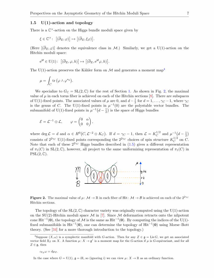
We specialize to GC = SL(2,C) for the rest of Section 1. As shown in Fig. 2, the maximalvalue of µ in each torus fiber is achieved on each of the Hitchin sections [8]. There are subspacesof U(1)-fixed points. The associated values of µ are 0, and d− 1

2 for d = 1, . . . , γC − 1, where γCis the genus of C. The U(1)-fixed points in µ−1(0) are the polystable vector bundles. Thesubmanifold of U(1)-fixed points in µ−1

(d− 1

2

)is the space of Higgs bundles

E = L−1 ⊕ L, ϕ =

(0 α0 0

),

where degL = d and α ∈ H0(C,L−2 ⊗ KC

). If d = γC − 1, then L = K

1/2C and µ−1

(d − 1

2

)consists of 22γC U(1)-fixed points corresponding the 22γC choices of spin structure K

1/2C on C.

Note that each of these 22γC Higgs bundles described in (1.5) gives a different representationof π1(C) in SL(2,C), however, all project to the same uniformizing representation of π1(C) inPSL(2,C).

Figure 2. The maximal value of µ : M→ R in each fiber of Hit : M→ B is achieved on each of the 22γC

Hitchin sections.

The topology of the SL(2,C) character variety was originally computed using the U(1)-actionon the SU(2)-Hitchin moduli space M in [7]. Since M deformation retracts onto the nilpotentcone Hit−1(0), the topology ofM is the same as Hit−1(0). By computing the indices of the U(1)-fixed submanifolds in Hit−1(0), one can determine the topology of Hit−1(0) using Morse–Botttheory. (See [34] for a more thorough introduction to the topology.)

4Suppose (X,ω) is a symplectic manifold with G-action. Then for any Z ∈ g = LieG, we get an associatedvector field XZ on X. A function µ : X → g∗ is a moment map for the G-action if µ is G-equivariant, and for allZ ∈ g, then

ιXZω = dµZ .

In the case where G = U(1), g = iR, so (ignoring i) we can view µ : X → R as an ordinary function.

8 L. Fredrickson

1.6 SL(2,R)-Higgs bundles

Recall, the nonabelian Hodge correspondence gives us the following equivalence:stable SL(2,C)-Higgs bundles

(∂E , ϕ)

/∼

←→

irreducible representationsρ : π1(C)→ SL(2,C)

/∼

.

One can define an SL(2,R)-Higgs bundle as a SL(2,C)-Higgs bundle which correspond toa SL(2,R)-representation:⋃

SL(2,R)-Higgs bundles

(∂E , ϕ)

/∼

←→

⋃irreducible representationsρ : π1(C)→ SL(2,R)

/∼.

The Lie subalgebra sl(2,R) ⊂ sl(2,C) is preserved by the map Φ→ Φ. Consequently, SL(2,R)-Higgs bundles can be viewed as SL(2,C)-Higgs bundles with additional conditions:

• E has an orthogonal structure Q : E → E∗, and

• ϕ is Q-symmetric, i.e., ϕTQ = Qϕ,

E E ⊗KC

E∗ E∗ ⊗KC .

ϕ

Q Q

ϕT

Note that the harmonic metric h will in turn satisfy hTQh = Q. We have already encounteredsome SL(2,R)-Higgs bundles. Namely, all Higgs bundles in the Hitchin sections are SL(2,R)-Higgs bundles. To see this, just take the orthogonal structure Q = ( 0 1

1 0 ) where the “1”s represent

the identity maps K1/2C →

(K−1/2C

)∗and K

−1/2C →

(K

1/2C

)∗.

2 The hyperkahler structure of the Hitchin moduli space

As a hyperkahler space, the Hitchin moduli space has a rich geometric structure. At least twoongoing lines of research motivate us to consider the hyperkahler geometry.

• There are many recent results about “branes” in Hitchin moduli space.

• There are recent results about the asymptotic geometry of the hyperkahler metric.

In this section, we give an introduction to hyperkahler geometry before specializing to thehyperkahler geometry of the Hitchin moduli space. An excellent additional reference is [33].

2.1 Introduction to hyperkahler geometry

A hyperkahler manifold is a manifold whose tangent space admits an action of I, J , K compatiblewith a single metric. To give a more precise definition of “hyperkahler”, we first have to define“Kahler”.

Definition 2.1. Let (X, I) be a complex manifold of dimCX = n.

• A hermitian metric on (X, I) is a Riemannian metric g such that g(v, w) = g(Iv, Iw).

Let ∇ denote the Levi-Civita connection5 on TX induced by g.

5Recall that the Levi-Civita connection on (X, g) is the unique connection that (1) preserves the metric, i.e.,∇g = 0 and (2) is torsion-free, i.e., for any vector fields ∇XY −∇YX = [X,Y ].

Perspectives on the Asymptotic Geometry of the Hitchin Moduli Space 9

• A hermitian metric g on (X, I) is Kahler if ∇I = 0.

• If (X, g, I) is Kahler, the Kahler form ω ∈ Ω1,1(X) is defined by ω(v, w) = g(Iv, w).

Example 2.2. C is Kahler. The complex structure I is given by multiplication by i, theRiemannian metric is g = dx2 + dy2 = dzdz, and the Kahler form is ω = dx ∧ dy = i

2dz ∧ dz.

It is easy to find examples of Kahler manifolds. For example, any complex submanifold ofCPn inherits a Kahler metric. Hyperkahler manifolds are much more rigid, so it is harder tofind examples.

Definition 2.3. A hyperkahler manifold is a tuple (X, g, I, J,K) where (X, g) is a Riemannianmanifold equipped with 3 complex structures I, J , K – obeying the usual quaternionic relations –such that (X, g, •) is Kahler, for • = I, J,K.

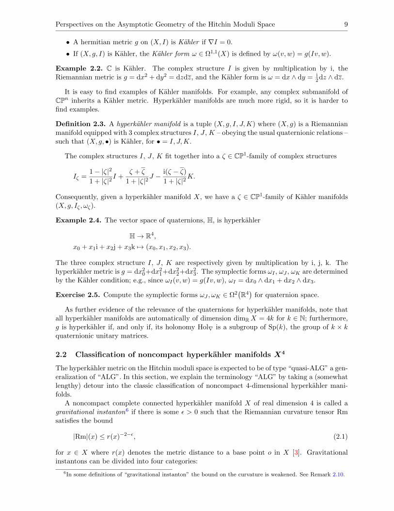
The complex structures I, J , K fit together into a ζ ∈ CP1-family of complex structures

Iζ =1− |ζ|2

1 + |ζ|2I +

ζ + ζ

1 + |ζ|2J − i(ζ − ζ)

1 + |ζ|2K.

Consequently, given a hyperkahler manifold X, we have a ζ ∈ CP1-family of Kahler manifolds(X, g, Iζ , ωζ).

Example 2.4. The vector space of quaternions, H, is hyperkahler

H→ R4,

x0 + x1i + x2j + x3k 7→ (x0, x1, x2, x3).

The three complex structure I, J , K are respectively given by multiplication by i, j, k. Thehyperkahler metric is g = dx2

0+dx21+dx2

2+dx23. The symplectic forms ωI , ωJ , ωK are determined

by the Kahler condition; e.g., since ωI(v, w) = g(Iv, w), ωI = dx0 ∧ dx1 + dx2 ∧ dx3.

Exercise 2.5. Compute the symplectic forms ωJ , ωK ∈ Ω2(R4)

for quaternion space.

As further evidence of the relevance of the quaternions for hyperkahler manifolds, note thatall hyperkahler manifolds are automatically of dimension dimRX = 4k for k ∈ N; furthermore,g is hyperkahler if, and only if, its holonomy Hol∇ is a subgroup of Sp(k), the group of k × kquaternionic unitary matrices.

2.2 Classification of noncompact hyperkahler manifolds X4

The hyperkahler metric on the Hitchin moduli space is expected to be of type “quasi-ALG” a gen-eralization of “ALG”. In this section, we explain the terminology “ALG” by taking a (somewhatlengthy) detour into the classic classification of noncompact 4-dimensional hyperkahler mani-folds.

A noncompact complete connected hyperkahler manifold X of real dimension 4 is called agravitational instanton6 if there is some ε > 0 such that the Riemannian curvature tensor Rmsatisfies the bound

|Rm|(x) ≤ r(x)−2−ε, (2.1)

for x ∈ X where r(x) denotes the metric distance to a base point o in X [3]. Gravitationalinstantons can be divided into four categories:

6In some definitions of “gravitational instanton” the bound on the curvature is weakened. See Remark 2.10.

10 L. Fredrickson

• ALE “asymptotically locally Euclidean” O(r4)

ex) H ' R4,• ALF “asymptotically locally flat” O

(r3)

ex) R3 × S1,• ALG [not an abbreviation] O

(r2)

ex) R2 × T 2,• ALH [not an abbreviation] O

(r1)

ex) R× T 3.Here, this coarse classification is by the dimension of the asymptotic tangent cone. The asymp-totic tangent cones are, respectively,• ALE C2/Γ where Γ is a finite subgroup of SU(2),• ALF R3 or R3/Z2,• ALG Cβ, where Cβ is a cone of angle 2πβ for β ∈ (0, 1],• ALH R+.

Within each broad category (ALE/ALF/ALG/ALH), we have a finer classification by geometrictype. Chen–Chen proved that any connected complete gravitational instanton with curvaturedecay like (2.1) must be asymptotic to some standard model. This is the data of a geometrictype [3]. For each geometric type, we have a moduli space of hyperkahler manifolds of that type.We will focus on the geometric classification for the cases ALE and ALG, since the ALE storyis classical and the ALG story is most relevant for the Hitchin moduli space.

The geometric classification of ALE hyperkahler metrics has been completed. The data forthe geometric type is a finite subgroup Γ of SU(2). Using this subgroup, define the singularspace

XΓ = C2/Γ.

Every ALE hyperkahler 4-manifold is diffeomorphic to the minimal resolution of XΓ for some Γ[26]. The moduli spaceMΓ of ALE instantons of type Γ is non-empty and is parameterized by theintegrals of the Kahler forms ωI , ωJ , ωK over the integer-valued second-homology lattice [25, 26].The asymptotic tangent cone of any X ∈MΓ is C2/Γ.

Example 2.6. Γ = Zk acts on (z = x0 + ix1, w = x2 + ix3) by (z, w) 7→(e2πi/kz, e2πi/kw

). The

moduli space MZkhas dimension 3k − 6 [19, 21].

For ALG gravitational instantons, the finer geometric classification is by the geometry atinfinity. These standard models are torus bundles over the flat cone Cβ of cone angle 2πβ ∈(0, 2π]. The list of torus bundles E → Cβ is quite restricted.

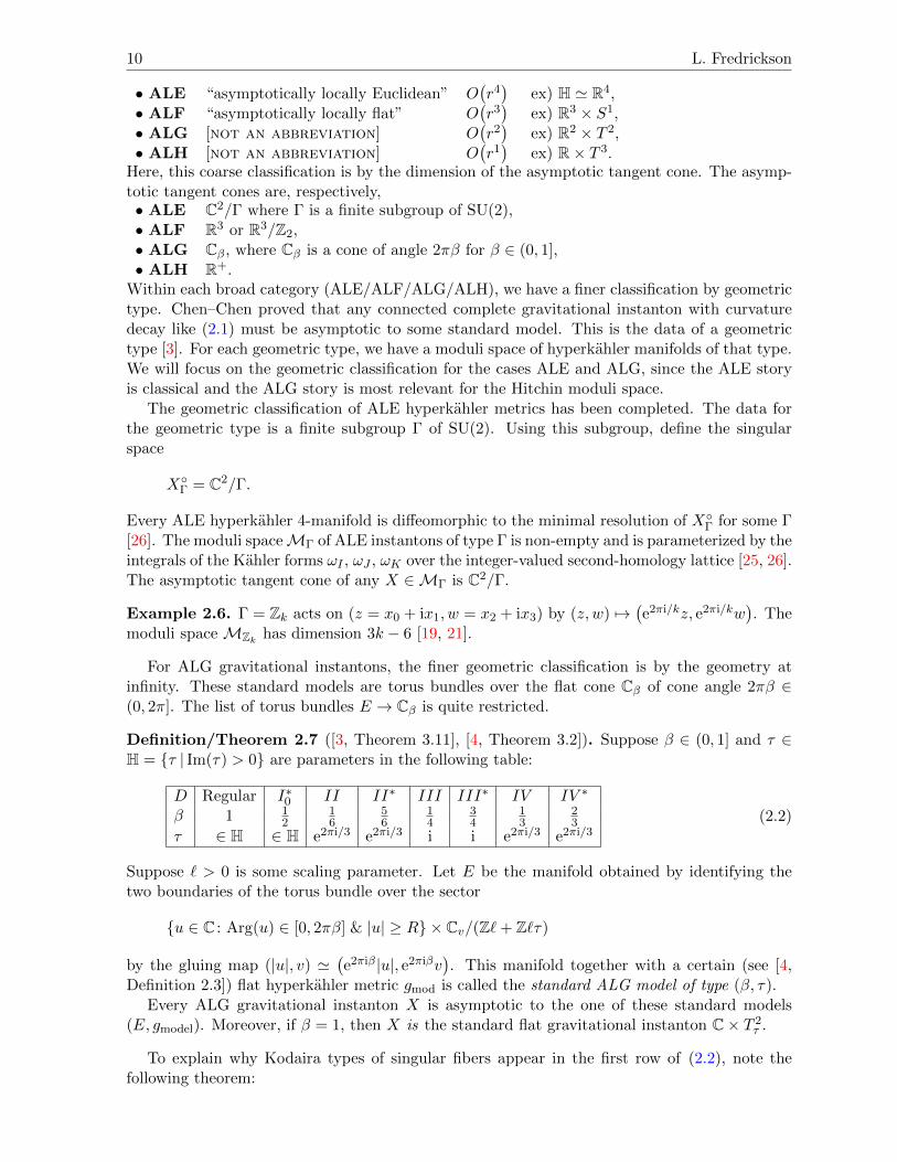
Definition/Theorem 2.7 ([3, Theorem 3.11], [4, Theorem 3.2]). Suppose β ∈ (0, 1] and τ ∈H = τ | Im(τ) > 0 are parameters in the following table:

D Regular I∗0 II II∗ III III∗ IV IV ∗

β 1 12

16

56

14

34

13

23

τ ∈ H ∈ H e2πi/3 e2πi/3 i i e2πi/3 e2πi/3(2.2)

Suppose ` > 0 is some scaling parameter. Let E be the manifold obtained by identifying thetwo boundaries of the torus bundle over the sector

u ∈ C : Arg(u) ∈ [0, 2πβ] & |u| ≥ R × Cv/(Z`+ Z`τ)

by the gluing map (|u|, v) '(e2πiβ|u|, e2πiβv

). This manifold together with a certain (see [4,

Definition 2.3]) flat hyperkahler metric gmod is called the standard ALG model of type (β, τ).Every ALG gravitational instanton X is asymptotic to the one of these standard models

(E, gmodel). Moreover, if β = 1, then X is the standard flat gravitational instanton C× T 2τ .

To explain why Kodaira types of singular fibers appear in the first row of (2.2), note thefollowing theorem:

Perspectives on the Asymptotic Geometry of the Hitchin Moduli Space 11

Theorem 2.8 ([3]). Any ALG gravitational instanton X can be compactified in a complexanalytic sense. I.e., there exists a compact elliptic surface7 X with a meromorphic functionψ : X → CP1 whose generic fiber is a complex torus. The fiber D = ψ−1(∞) is either regularor singular of Kodaira type I∗0 , II, II∗, III, III∗, IV , IV ∗. Moreover, there is some ζ ∈ CP1

such that (X, Iζ) is biholomorphic to X −D.

Remark 2.9. Looking forward, this fibration ψ should loosely remind you of the Hitchin fibra-tion Hit : M→ B ' C

12

dimCM.

Remark 2.10. There are other definitions of gravitational instantons appearing in the literaturewithout the strict curvature bounds in (2.1). Stranger things can happen if we remove thesecurvature bounds. Given any noncompact complete connected hyperkahler manifold X of realdimension 4, one can associate a number based on the asymptotic volume growth of Br, a ballof radius r. With the definition of gravitational instantons in (2.1), the volume growth is aninteger: 4, 3, 2, 1. Without the curvature bounds in (2.1), the volume growth need not be aninteger. There are no hyperkahler metrics with growth between r3 and r4 [29]. However, Heinconstructed an example of a hyperkahler metric with volume growth r4/3 [20]. Chen–Chen callthis an example of type ALG∗ since the growth rate 4

3 is the in ALG-like interval (1, 2]. The “∗”indicates that the modulus of the torus fibers is changing; it is unbounded asymptotically, i.e.,the torus fiber is becoming very long and thin.

2.3 The hyperkahler metric on the Hitchin moduli space

The Hitchin moduli space has a hyperkahler metric. To hint at the origins of the hyperkahlerstructure, we instead discuss the origin of the CP1-family of complex structures on the Hitchinmoduli space. The CP1-family of complex structures arises from the complex structure on theRiemann surface C and the complex structure on the group GC; these respectively, give the Iand J complex structures on M.

Each of these complex structures Iζ gives an avatar of the Hitchin moduli space as a complexmanifold:

• Mζ=0 = (M, Iζ=0) is the Higgs bundle moduli space;

• Mζ∈C× is the moduli space of flat connections;

• Mζ=∞ is the moduli space of anti-Higgs bundles.

Note that these can be genuinely different as complex manifolds. For M =M(T 2τ ,GL(1,C)

),

M0 ' C× T 2τ , Mζ∈C× ' C× × C×, M∞ ' C× T 2

−τ , (2.3)

where T 2τ = C/(Z ⊕ τZ) is the complex torus with parameter τ . The hyperkahler metric on

M0 ' R2x0,x1 × T

2x3,x4 is g = dx2

0 + dx21 + dx2

2 + dx23, which is indeed ALG.

In general, the hyperkahler metric on Hitchin moduli space is expected to be of type “quasi-ALG” which is some generalization8 of ALG. In higher dimensions “ALG” has not be formally

7Furthermore, from [4, Theorem 1.3], ψ : X → CP1 is a rational elliptic surface in the sense of [4, Definition 2.7]8This term “QALG” has not been formally defined, but QALG is supposed to generalize ALG in an analogous

way as QALE generalizes ALE and QAC generalizes AC.Dominic Joyce considered a higher-dimensional version of ALE, and subsequently defined QALE. In this context,

a (Q)ALE metric is a Kahler metric on a manifold of real-dimension 2n with asymptotic volume growth like r2n.Fix a finite subgroup Γ ⊂ U(n). If Γ acts freely on Cn − 0, then Cn/Γ has an isolated quotient singularityat 0. The appropriate class of Kahler metrics on the resolution X of Cn/Γ [23] are ALE metrics. If however,Γ does not act freely, then the singularities of Cn/Γ extend to the ends. The appropriate class of Kahler metricson resolution X of non-isolated quotient singularities are called quasi-ALE or QALE [24].

For quasi-asymptotically conical (QAC) versus AC, see for example [5].

12 L. Fredrickson

defined; however, by analogy with the 4-dimensional case described in Section 2.2, any higher-dimensional ALG hyperkahler manifold should be asymptotic to a flat torus bundle over a half-dimensional complex vector space. Moreover, the modulus of the torus lattice should staybounded. (This condition on the modulus rules out higher-dimensional generalizations of Hein’sALG∗ example in Remark 2.10.)

For the Hitchin moduli space, the Hitchin fibration Hit : M → B should asymptoticallygive the torus fibration over a half-dimensional complex vector space. It certainly does in theALG example of (2.3)! Because the singular locus typically intersects the ends of the Hitchinbase B, we will typically not have a nondegenerate asymptotic torus fibration ψ : M → B.Consequently, in these cases, the Hitchin moduli space is instead expected to be “QALG”, asdescribed in footnote 8, rather than ALG.

2.4 The hyperkahler metric

Alternatively, the Hitchin moduli space can be viewed as pairs[(∂A,Φ)

]solving Hitchin’s equa-

tions given a fixed complex vector bundle E → C with fixed hermitian metric. Once we’vefixed a hermitian metric, we only consider gauge transformations which fix the hermitian met-ric. This gives a reduction from complex gauge transformations GC = GL(E) to unitary gaugetransformations G = U(E)-gauge transformations.

The hyperkahler metric onM is defined using the unitary formulation of Hitchin’s equationsin terms of pairs (∂A,Φ). First, consider the configuration space C of all pairs (∂A,Φ) solvingHitchin’s equations – without taking gauge equivalence. The space of holomorphic structureson E is an affine space modeled on Ω0,1(C,EndE). The space of all Higgs fields is the vectorspace Ω1,0(C,EndE). Thus, the set of pairs (∂A,Φ) solving Hitchin’s equations sits inside anaffine space modeled on

Ω0,1(C,EndE)× Ω1,0(C,EndE).

This product space has a natural L2-metric given by

g((A0,1

1 , Φ1

),(A0,1

2 , Φ2

))= 2i

∫C

⟨Φ1∧, Φ2

⟩−⟨A0,1

1∧, A0,1

2

⟩,

where the hermitian inner products are taken only on the matrix-valued piece, so that 〈Φ1∧, Φ2〉

is a (1, 1)-form. The factor 2i appears since dz ∧ dz = −2idx ∧ dy. The hyperkahler metric gMon M descends from this L2-metric g. Note that any tangent vector [(A0,1, Φ)] ∈ T[(∂A,Φ)]Mhas multiple representatives. The hyperkahler metric gM on M is defined so that

‖[(A0,1, Φ)]‖gM = min(A0,1,Φ)∈[(A0,1,Φ)]

‖(A0,1, Φ)‖g.

The minimizing representative is said to be in “Coulomb gauge”. We will call this naturalhyperkahler metric gM “Hitchin’s hyperkahler L2-metric”.

2.5 Branes in the Hitchin moduli space

Recently, there have been a number of results about branes in the Hitchin moduli space. (See [1]for a survey of results and further directions.)

Definition 2.11. A brane is an object in one of the following categories:

• [A-side, i.e., symplectic] Fukaya category, or

• [B-side, i.e., complex] derived category of coherent sheaves.

Perspectives on the Asymptotic Geometry of the Hitchin Moduli Space 13

The approximate data of an (A/B)-brane in a (symplectic/complex) manifold X is

• a submanifold Y ⊂ X, together with

• (E,∇)→ Y , a vector bundle with connection.

Further ignoring bundles, an A-brane in a symplectic manifold (X,ω) “is” a Lagrangian sub-manifold9 of X. A B-brane in a complex manifold (X, I) “is” a holomorphic submanifold.

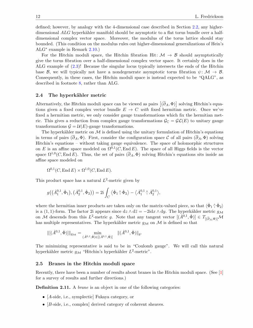
If X is hyperkahler, then X has a triple of Kahler structures (X, g, I, ωI , J, ωJ ,K, ωK). Withrespect to the triple of Kahler structures, a (B,A,A) brane in X “is” a submanifold Y whichis holomorphic with respect to I, Lagrangian with respect to ωJ , and Lagrangian with respectto ωK . Not all types exis – only (B,A,A), (A,B,A), (A,A,B) and (B,B,B)-branes exist.

Given a (B,A,A) brane Y ⊂ X, one might ask whether the submanifold Y is holomorphicwith respect to Iζ or Lagrangian with respect to ωζ for any of the other Kahler structures(X, g, Iζ , ωζ). In fact, as shown in Fig. 3, Y is holomorphic with respect to both ±I, and Y isLagrangian for |ζ| = 1 – the whole circle containing J and K. It is neither holomorphic, norLagrangian for any other value ζ. Similar statements hold for (A,B,A) and (A,A,B) branes.

Figure 3. (B,A,A)-brane.

Exercise 2.12. Let Y be the (x0, x1)-plane in quaternion space.

(a) Show that Y is (the support of) a (B,A,A) brane, i.e., it’s holomorphic with respect to Iand Lagrangian with respect to ωJ and ωK .

(b) Is Y holomorphic with respect to any other complex structure Iζ? Is Y Lagrangian withrespect to any other symplectic structure ωζ?

Many recent results concern constructions of different families of branes inside the Hitchinmoduli space. For example, some branes – including the Hitchin section, which is a (B,A,A)-brane – are constructed as fixed point sets of certain involutions on the moduli space of Higgsbundles. (See, for example, [2]). Langlands duality, shown in (2.4), exchanges the brane types.For example, (B,A,A)-branes in the G-Hitchin moduli space MG get mapped to (B,B,B)-branes in the LG-Hitchin moduli space MLG

MG MLG

BG ' BLG.

(2.4)

3 Spectral interpretation and limiting configurations

In Section 1.4, we introduced the Hitchin fibration. Now, we

1) give a geometric interpretation of the Hitchin fibration, and

2) give a construction of the harmonic metric for a Higgs bundle near the ends of the modulispace.

9Let (X,ω) be a symplectic manifold. Recall a submanifold L is Lagrangian if dimR L = 12

dimRX and ω|L = 0.

14 L. Fredrickson

3.1 Spectral data

The Hitchin fibration, introduced in (1.3), is a map

Hit : M B ' C12

dimCM,(∂E , ϕ, h

)7→ charϕ(λ),

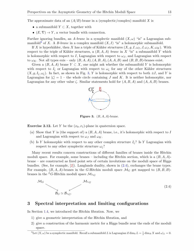
where the characteristic polynomial charϕ λ encodes the eigenvalues λ1, . . . , λn of ϕ. There aretwo additional interpretations of B that are useful:

Figure 4. Hitchin fibration.

• [algebraic interpretation] The coefficients of

charϕ(λ) = λn + q1λn−1 + q2λ

n−2 + · · ·+ qn−1λ+ qn

are sections qi ∈ H0(C,Ki

C

). Consequently, the Hitchin base B can be identified with the

complex vector space of coefficients of charϕ(λ). For example,

BGL(n,C) =n⊕i=1

H0(C,Ki

C

)3 (q1, . . . , qn), and

BSL(n,C) =n⊕i=2

H0(C,Ki

C

)3 (q2, . . . , qn),

since for SL(n,C), q1 = − trϕ = 0.

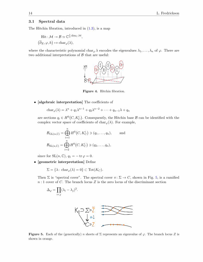
• [geometric interpretation] Define

Σ = λ : charϕ(λ) = 0 ⊂ Tot(KC).

Then Σ is “spectral cover”. The spectral cover π : Σ → C, shown in Fig. 5, is a ramifiedn : 1 cover of C. The branch locus Z is the zero locus of the discriminant section

∆ϕ =∏i<j

(λi − λj)2.

Figure 5. Each of the (generically) n sheets of Σ represents an eigenvalue of ϕ. The branch locus Z is

shown in orange.

Perspectives on the Asymptotic Geometry of the Hitchin Moduli Space 15

For GL(n,C) and SL(n,C)-Higgs bundles, the regular locus M′, discussed in Section 1.4,consists of Higgs bundles lying over smooth spectral covers Σ.

Exercise 3.1.

(a) What bundle is the discriminant section ∆ϕ a section of? What is the number of zerosof ∆ϕ with multiplicity?

(b) Use this to compute the number of ramification points of π : Σ→ C (with multiplicity).

(c) Compute the genus of Σ.Hint: In the case of unramified N : 1 covers π : S′ → S, the Riemann–Hurwitz formulasays that χ(S′) = Nχ(S) where χ(S) = 2(γS − 1) is the Euler characteristic and γS is thegenus of S. In the case of ramified covers, this is corrected to

χ(S′) = Nχ(S)−∑P∈Z

(eP − 1),

where Z ⊂ S′ is the set of points of S′ where π locally looks like π(z) = zeP . The number ePis called the “ramification index”.

Fact 3.2. For SL(2,C), Hit :(∂E , ϕ, h

)7→ detϕ = q2, so the branch locus Z is the set of zeros

of detϕ. Call p ∈ Z a simple zero if q2 ∼ zdz2, and call p a kth order zero if q2 ∼ zkdz2. ForMSL(2,C), q2 has only simple zeros ⇔ Σ is smooth ⇔ the spectral cover Σ lies in the regular

locus B′ = B − Bsing ⇔ Hit−1(Σ) is a compact abelian variety.

Having given a geometric interpretation of the Hitchin base B, we now give a geometric inter-pretation of the torus fibers of Hit : M′ → B′. (We restrict to the regular locus M′ → B′ sincethe torus fibers degenerate over the singular locus Bsing.) As shown in Fig. 6, the eigenspacesof a Higgs field ϕ can be encoded in a line bundle L → Σ. Note that E ' π∗L. The torus fiberHit−1(Σ) is some space of line bundles over the spectral cover Σ. For GL(n,C), this fiber is theJacobian, Jac(Σ). For SL(n,C), this fiber is the Prym variety Prym(Σ, C). Here, we have a sub-variety of the Jacobian because of the trivialization of determinant as Det(π∗L) ' Det E ' O.

Figure 6. Each sheet of the spectral cover Σ → C over a point x ∈ C corresponds to an eigenvalue

of ϕ(x). The fiber of the spectral line bundle L is the associated eigenspace of ϕ(x).

3.2 Limits in the Hitchin moduli space

In [17, 18], Gaiotto–Moore–Neitzke give a conjectural description of the hyperkahler metric gM.Gaiotto–Moore–Neitzke’s conjecture suggests that – surprisingly – much of the asymptotic geo-metry of M can be derived from the abelian data L → Σ. (We give a survey of this conjectureand recent progress in Section 4.) In this section, we describe how solutions of Hitchin’s equationsat the ends of the moduli space come naturally from the abelian data L → Σ. This is an earlyhint of the importance of the abelian data for the asymptotic geometry of the Hitchin modulispace.

16 L. Fredrickson

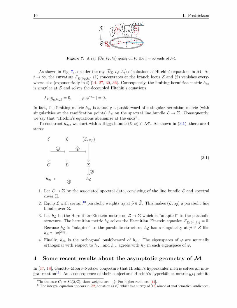
Figure 7. A ray(∂E , tϕ, ht

)going off to the t =∞ ends of M.

As shown in Fig. 7, consider the ray(∂E , tϕ, ht

)of solutions of Hitchin’s equations inM. As

t→∞, the curvature FD(∂E ,ht)(1) concentrates at the branch locus Z and (2) vanishes every-

where else (exponentially in t) [14, 27, 30, 36]. Consequently, the limiting hermitian metric h∞is singular at Z and solves the decoupled Hitchin’s equations

FD(∂E ,h∞) = 0, [ϕ,ϕ∗h∞ ] = 0.

In fact, the limiting metric h∞ is actually a pushforward of a singular hermitian metric (withsingularities at the ramification points) hL on the spectral line bundle L → Σ. Consequently,we say that “Hitchin’s equations abelianize at the ends”.

To construct h∞, we start with a Higgs bundle (E , ϕ) ∈ M′. As shown in (3.1), there are 4steps:

E L (L, αp)

C Σ Σ

h∞ hL

1© 2©

3©

4©

(3.1)

1. Let L → Σ be the associated spectral data, consisting of the line bundle L and spectralcover Σ.

2. Equip L with certain10 parabolic weights αp at p ∈ Z. This makes (L, αp) a parabolic linebundle over Σ.

3. Let hL be the Hermitian–Einstein metric on L → Σ which is “adapted” to the parabolicstructure. The hermitian metric hL solves the Hermitian–Einstein equation FD(∂L,h`)

= 0.

Because hL is “adapted” to the parabolic structure, hL has a singularity at p ∈ Z likehL ' |w|2αp .

4. Finally, h∞ is the orthogonal pushforward of hL. The eigenspaces of ϕ are mutuallyorthogonal with respect to h∞, and h∞ agrees with hL in each eigenspace of ϕ.

4 Some recent results about the asymptotic geometry of MIn [17, 18], Gaiotto–Moore–Neitzke conjecture that Hitchin’s hyperkahler metric solves an inte-gral relation11. As a consequence of their conjecture, Hitchin’s hyperkahler metric gM admits

10In the case GC = SL(2,C), these weights are − 12. For higher rank, see [14].

11The integral equation appears in [32, equation (4.8)] which is a survey of [18] aimed at mathematical audiences.

Perspectives on the Asymptotic Geometry of the Hitchin Moduli Space 17

an expansion in terms of a simpler hyperkahler metric gsf , known as the “semiflat metric”. Thesemiflat metric gsf is smooth on M′ and exists because M is a algebraic completely integrablesystem [16, Theorem 3.8]. Thus it is deeply related to the spectral data.

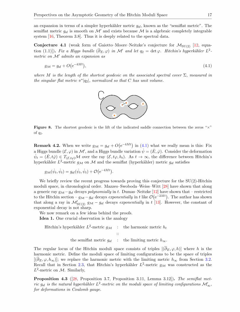
Conjecture 4.1 (weak form of Gaiotto–Moore–Neitzke’s conjecture for MSU(2) [12, equa-

tion (1.1)]). Fix a Higgs bundle (∂E , ϕ) in M′ and let q2 = detϕ. Hitchin’s hyperkahler L2-metric on M′ admits an expansion as

gM = gsf +O(e−4Mt

), (4.1)

where M is the length of the shortest geodesic on the associated spectral cover Σ, measured inthe singular flat metric π∗|q2|, normalized so that C has unit volume.

Figure 8. The shortest geodesic is the lift of the indicated saddle connection between the zeros “×”

of q2.

Remark 4.2. When we write gM = gsf + O(e−4Mt

)in (4.1) what we really mean is this: Fix

a Higgs bundle (E , ϕ) inM′, and a Higgs bundle variation ψ = (E, ϕ). Consider the deformationψt = (E, tϕ) ∈ T(E,tϕ)M over the ray (E , tϕ, ht). As t → ∞, the difference between Hitchin’shyperkahler L2-metric gM on M and the semiflat (hyperkahler) metric gsf satisfies

gM(ψt, ψt) = gsf(ψt, ψt) +O(e−4Mt

).

We briefly review the recent progress towards proving this conjecture for the SU(2)-Hitchinmoduli space, in chronological order. Mazzeo–Swoboda–Weiss–Witt [28] have shown that alonga generic ray gM−gsf decays polynomially in t. Dumas–Neitzke [12] have shown that – restrictedto the Hitchin section – gM−gsf decays exponentially in t like O

(e−2Mt

). The author has shown

that along a ray in M′SU(2) gM − gsf decays exponentially in t [13]. However, the constant ofexponential decay is not sharp.

We now remark on a few ideas behind the proofs.Idea 1. One crucial observation is the analogy

Hitchin’s hyperkahler L2-metric gM : the harmonic metric ht

::

the semiflat metric gsf : the limiting metric h∞.

The regular locus of the Hitchin moduli space consists of triples [(∂E , ϕ, h)] where h is theharmonic metric. Define the moduli space of limiting configurations to be the space of triples[(∂E , ϕ, h∞)]; we replace the harmonic metric with the limiting metric h∞ from Section 3.2.Recall that in Section 2.3, that Hitchin’s hyperkahler L2-metric gM was constructed as theL2-metric on M. Similarly,

Proposition 4.3 ([28, Proposition 3.7, Proposition 3.11, Lemma 3.12]). The semiflat met-ric gsf is the natural hyperkahler L2-metric on the moduli space of limiting configurations M′∞,for deformations in Coulomb gauge.

18 L. Fredrickson

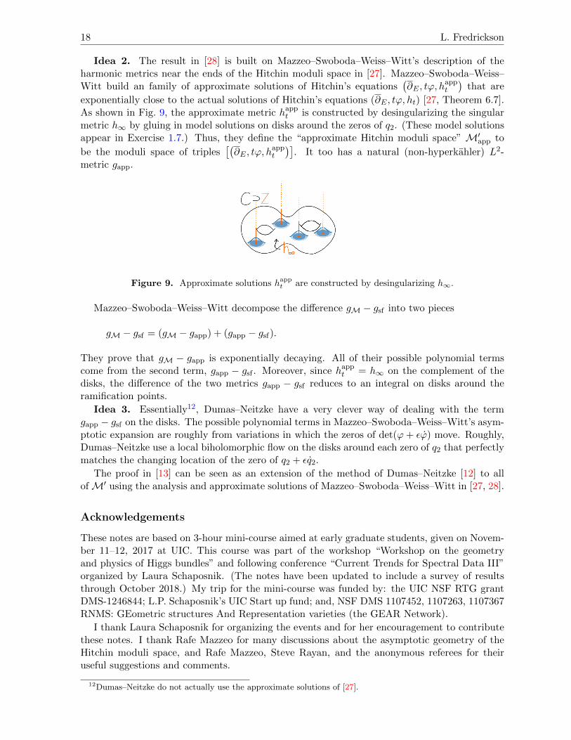
Idea 2. The result in [28] is built on Mazzeo–Swoboda–Weiss–Witt’s description of theharmonic metrics near the ends of the Hitchin moduli space in [27]. Mazzeo–Swoboda–Weiss–Witt build an family of approximate solutions of Hitchin’s equations

(∂E , tϕ, h

appt

)that are

exponentially close to the actual solutions of Hitchin’s equations (∂E , tϕ, ht) [27, Theorem 6.7].As shown in Fig. 9, the approximate metric happ

t is constructed by desingularizing the singularmetric h∞ by gluing in model solutions on disks around the zeros of q2. (These model solutionsappear in Exercise 1.7.) Thus, they define the “approximate Hitchin moduli space” M′app to

be the moduli space of triples[(∂E , tϕ, h

appt

)]. It too has a natural (non-hyperkahler) L2-

metric gapp.

Figure 9. Approximate solutions happt are constructed by desingularizing h∞.

Mazzeo–Swoboda–Weiss–Witt decompose the difference gM − gsf into two pieces

gM − gsf = (gM − gapp) + (gapp − gsf).

They prove that gM − gapp is exponentially decaying. All of their possible polynomial termscome from the second term, gapp − gsf . Moreover, since happ

t = h∞ on the complement of thedisks, the difference of the two metrics gapp − gsf reduces to an integral on disks around theramification points.

Idea 3. Essentially12, Dumas–Neitzke have a very clever way of dealing with the termgapp − gsf on the disks. The possible polynomial terms in Mazzeo–Swoboda–Weiss–Witt’s asym-ptotic expansion are roughly from variations in which the zeros of det(ϕ+ εϕ) move. Roughly,Dumas–Neitzke use a local biholomorphic flow on the disks around each zero of q2 that perfectlymatches the changing location of the zero of q2 + εq2.

The proof in [13] can be seen as an extension of the method of Dumas–Neitzke [12] to allofM′ using the analysis and approximate solutions of Mazzeo–Swoboda–Weiss–Witt in [27, 28].

Acknowledgements

These notes are based on 3-hour mini-course aimed at early graduate students, given on Novem-ber 11–12, 2017 at UIC. This course was part of the workshop “Workshop on the geometryand physics of Higgs bundles” and following conference “Current Trends for Spectral Data III”organized by Laura Schaposnik. (The notes have been updated to include a survey of resultsthrough October 2018.) My trip for the mini-course was funded by: the UIC NSF RTG grantDMS-1246844; L.P. Schaposnik’s UIC Start up fund; and, NSF DMS 1107452, 1107263, 1107367RNMS: GEometric structures And Representation varieties (the GEAR Network).

I thank Laura Schaposnik for organizing the events and for her encouragement to contributethese notes. I thank Rafe Mazzeo for many discussions about the asymptotic geometry of theHitchin moduli space, and Rafe Mazzeo, Steve Rayan, and the anonymous referees for theiruseful suggestions and comments.

12Dumas–Neitzke do not actually use the approximate solutions of [27].

Perspectives on the Asymptotic Geometry of the Hitchin Moduli Space 19

References

[1] Anderson L.B., Esole M., Fredrickson L., Schaposnik L.P., Singular geometry and Higgs bundles in stringtheory, SIGMA 14 (2018), 037, 27 pages, arXiv:1710.0845.

[2] Baraglia D., Schaposnik L.P., Real structures on moduli spaces of Higgs bundles, Adv. Theor. Math. Phys.20 (2016), 525–551, arXiv:1309.1195.

[3] Chen G., Chen X., Gravitational instantons with faster than quadratic decay (I), arXiv:1505.01790.

[4] Chen G., Chen X., Gravitational instantons with faster than quadratic decay (III), arXiv:1603.08465.

[5] Conlon R.J., Degeratu A., Rochon F., Quasi-asymptotically conical Calabi–Yau manifolds,arXiv:1611.04410.

[6] Corlette K., Flat G-bundles with canonical metrics, J. Differential Geom. 28 (1988), 361–382.

[7] Daskalopoulos G.D., Wentworth R.A., Wilkin G., Cohomology of SL(2,C) character varieties of surfacegroups and the action of the Torelli group, Asian J. Math. 14 (2010), 359–383, arXiv:0808.0131.

[8] Deroin B., Tholozan N., Dominating surface group representations by Fuchsian ones, Int. Math. Res. Not.2016 (2016), 4145–4166, arXiv:1311.2919.

[9] Donagi R., Markman E., Spectral covers, algebraically completely integrable, Hamiltonian systems, andmoduli of bundles, in Integrable Systems and Quantum Groups (Montecatini Terme, 1993), Lecture Notesin Math., Vol. 1620, Springer, Berlin, 1996, 1–119, arXiv:alg-geom/9507017.

[10] Donaldson S.K., A new proof of a theorem of Narasimhan and Seshadri, J. Differential Geom. 18 (1983),269–277.

[11] Donaldson S.K., Twisted harmonic maps and the self-duality equations, Proc. London Math. Soc. 55 (1987),127–131.

[12] Dumas D., Neitzke A., Asymptotics of Hitchin’s metric on the Hitchin section, Comm. Math. Phys., toappear, arXiv:1802.07200.

[13] Fredrickson L., Exponential decay for the asymptotic geometry of the Hitchin metric, arXiv:1810.01554.

[14] Fredrickson L., Generic ends of the moduli space of SL(n,C)-Higgs bundles, arXiv:1810.01556.

[15] Fredrickson L., Neitzke A., From S1-fixed points to W-algebra representations, arXiv:1709.06142.

[16] Freed D.S., Special Kahler manifolds, Comm. Math. Phys. 203 (1999), 31–52, arXiv:hep-th/9712042.

[17] Gaiotto D., Moore G.W., Neitzke A., Four-dimensional wall-crossing via three-dimensional field theory,Comm. Math. Phys. 299 (2010), 163–224, arXiv:0807.4723.

[18] Gaiotto D., Moore G.W., Neitzke A., Wall-crossing, Hitchin systems, and the WKB approximation, Adv.Math. 234 (2013), 239–403, arXiv:0907.3987.

[19] Gibbons G.W., Hawking S.W., Gravitational multi-instantons, Phys. Lett. B 78 (1978), 430–432.

[20] Hein H.-J., Gravitational instantons from rational elliptic surfaces, J. Amer. Math. Soc. 25 (2012), 355–393.

[21] Hitchin N.J., Polygons and gravitons, Math. Proc. Cambridge Philos. Soc. 85 (1979), 465–476.

[22] Hitchin N.J., The self-duality equations on a Riemann surface, Proc. London Math. Soc. 55 (1987), 59–126.

[23] Joyce D., Asymptotically locally Euclidean metrics with holonomy SU(m), Ann. Global Anal. Geom. 19(2001), 55–73, arXiv:math.AG/9905041.

[24] Joyce D., Quasi-ALE metrics with holonomy SU(m) and Sp(m), Ann. Global Anal. Geom. 19 (2001), 103–132, arXiv:math.AG/9905043.

[25] Kronheimer P.B., The construction of ALE spaces as hyper-Kahler quotients, J. Differential Geom. 29(1989), 665–683.

[26] Kronheimer P.B., A Torelli-type theorem for gravitational instantons, J. Differential Geom. 29 (1989),685–697.

[27] Mazzeo R., Swoboda J., Weiss H., Witt F., Ends of the moduli space of Higgs bundles, Duke Math. J. 165(2016), 2227–2271, arXiv:1405.5765.

[28] Mazzeo R., Swoboda J., Weiss H., Witt F., Asymptotic geometry of the Hitchin metric, arXiv:1709.03433.

[29] Minerbe V., On the asymptotic geometry of gravitational instantons, Ann. Sci. Ec. Norm. Super. (4) 43(2010), 883–924.

[30] Mochizuki T., Asymptotic behaviour of certain families of harmonic bundles on Riemann surfaces, J. Topol.9 (2016), 1021–1073, arXiv:1508.05997.

20 L. Fredrickson

[31] Narasimhan M.S., Seshadri C.S., Stable and unitary vector bundles on a compact Riemann surface, Ann.of Math. 82 (1965), 540–567.

[32] Neitzke A., Notes on a new construction of hyperkahler metrics, arXiv:1308.2198.

[33] Neitzke A., Moduli of Higgs bundles, 2016, available at http://www.ma.utexas.edu/users/neitzke/

teaching/392C-higgs-bundles/higgs-bundles.pdf.

[34] Rayan S., Aspects of the topology and combinatorics of Higgs bundle moduli spaces, SIGMA 14 (2018),129, 18 pages, arXiv:1809.05732.

[35] Simpson C.T., Higgs bundles and local systems, Inst. Hautes Etudes Sci. Publ. Math. (1992), 5–95.

[36] Taubes C.H., PSL(2;C) connections on 3-manifolds with L2 bounds on curvature, Camb. J. Math. 1 (2013),239–397, arXiv:1205.0514.

[37] Wentworth R.A., Higgs bundles and local systems on Riemann surfaces, in Geometry and Quantiza-tion of Moduli Spaces, Adv. Courses Math. CRM Barcelona, Birkhauser/Springer, Cham, 2016, 165–219,arXiv:1402.4203.

[38] Wolf M., The Teichmuller theory of harmonic maps, J. Differential Geom. 29 (1989), 449–479.