Copyright © Cengage Learning. All rights reserved.

14.4 Tangent Planes andLinear Approximations

2

Tangent PlanesSuppose a surface S has equation z = f (x, y), where f hascontinuous first partial derivatives, and let P(x0, y0, z0) be apoint on S.

Let C1 and C2 be the curves obtained by intersecting thevertical planes y = y0 and x = x0 with the surface S. Thenthe point P lies on both C1 and C2.

Let T1 and T2 be the tangent lines to the curves C1 and C2at the point P.

3

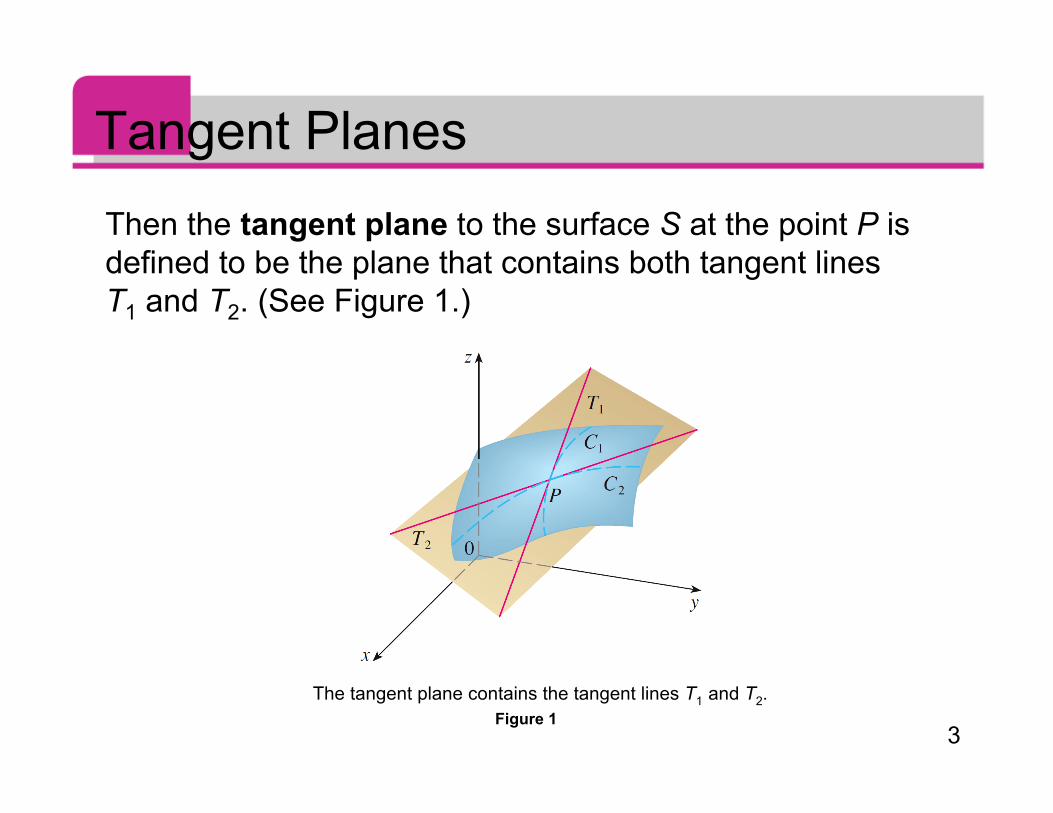
Tangent PlanesThen the tangent plane to the surface S at the point P isdefined to be the plane that contains both tangent linesT1 and T2. (See Figure 1.)

Figure 1The tangent plane contains the tangent lines T1 and T2.

4

Tangent PlanesIf C is any other curve that lies on the surface S andpasses through P, then its tangent line at P also lies in thetangent plane.

Therefore you can think of the tangent plane to S at P asconsisting of all possible tangent lines at P to curves that lieon S and pass through P. The tangent plane at P is theplane that most closely approximates the surface S nearthe point P. We know that any plane passing through thepoint P(x0, y0, z0) has an equation of the form

A (x – x0) + B (y – y0) + C (z – z0) = 0

5

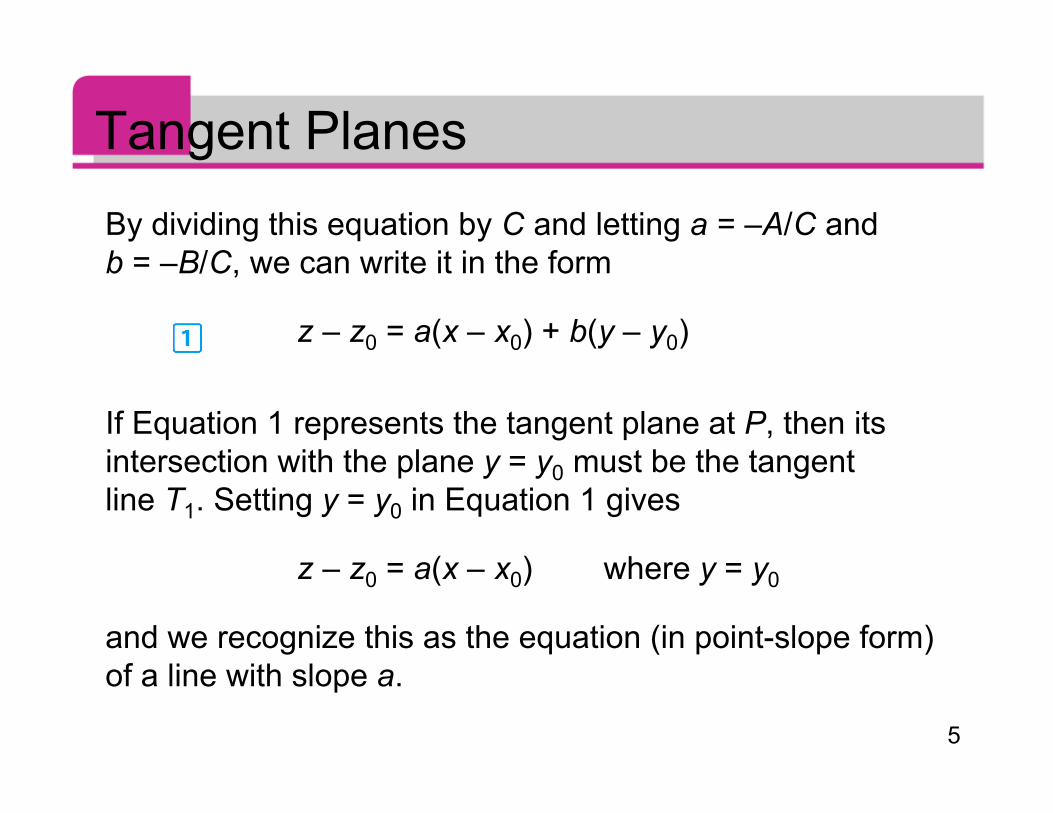
Tangent PlanesBy dividing this equation by C and letting a = –A/C andb = –B/C, we can write it in the form

z – z0 = a(x – x0) + b(y – y0)

If Equation 1 represents the tangent plane at P, then itsintersection with the plane y = y0 must be the tangentline T1. Setting y = y0 in Equation 1 gives

z – z0 = a(x – x0) where y = y0

and we recognize this as the equation (in point-slope form)of a line with slope a.

6

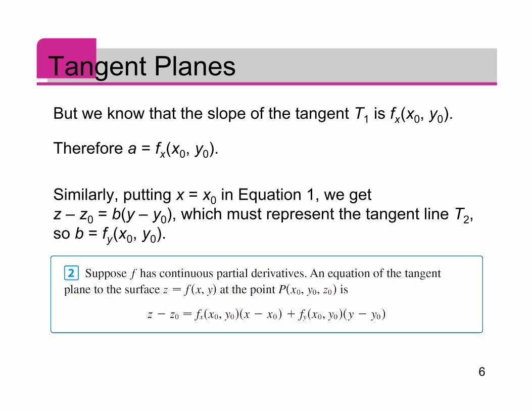
Tangent PlanesBut we know that the slope of the tangent T1 is fx (x0, y0).

Therefore a = fx (x0, y0).

Similarly, putting x = x0 in Equation 1, we getz – z0 = b(y – y0), which must represent the tangent line T2,so b = fy (x0, y0).

7

Example 1Find the tangent plane to the elliptic paraboloid z = 2x2 + y2

at the point (1, 1, 3).

Solution:Let f (x, y) = 2x2 + y2.Then fx(x, y) = 4x fy(x, y) = 2y fx(1, 1) = 4 fy(1, 1) = 2

Then (2) gives the equation of the tangent plane at(1, 1, 3) as

z – 3 = 4(x – 1) + 2(y – 1)or z = 4x + 2y – 3

8

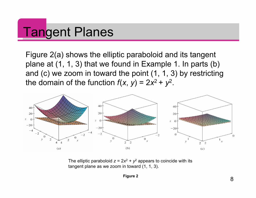
Tangent PlanesFigure 2(a) shows the elliptic paraboloid and its tangentplane at (1, 1, 3) that we found in Example 1. In parts (b)and (c) we zoom in toward the point (1, 1, 3) by restrictingthe domain of the function f (x, y) = 2x2 + y2.

Figure 2

The elliptic paraboloid z = 2x2 + y2 appears to coincide with its tangent plane as we zoom in toward (1, 1, 3).

9

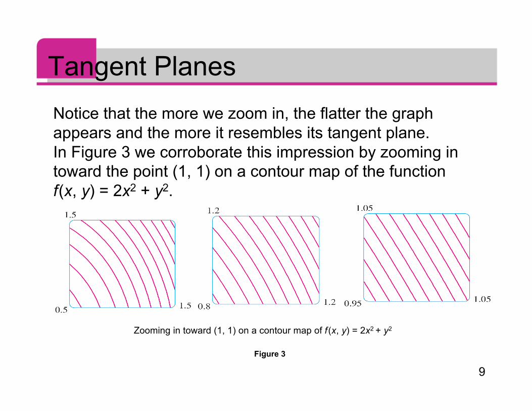
Tangent PlanesNotice that the more we zoom in, the flatter the graphappears and the more it resembles its tangent plane.In Figure 3 we corroborate this impression by zooming intoward the point (1, 1) on a contour map of the functionf (x, y) = 2x2 + y2.

Figure 3

Zooming in toward (1, 1) on a contour map of f (x, y) = 2x2 + y2

10

Tangent PlanesNotice that the more we zoom in, the more the level curveslook like equally spaced parallel lines, which ischaracteristic of a plane.

11

Linear ApproximationsIn Example 1 we found that an equation of the tangentplane to the graph of the function f (x, y) = 2x2 + y2 at thepoint (1, 1, 3) is z = 4x + 2y – 3. Therefore, the linearfunction of two variables

L(x, y) = 4x + 2y – 3

is a good approximation to f (x, y) when (x, y) is near (1, 1).The function L is called the linearization of f at (1, 1) andthe approximation

f (x, y) ≈ 4x + 2y – 3

is called the linear approximation or tangent planeapproximation of f at (1, 1).

12

Linear ApproximationsFor instance, at the point (1.1, 0.95) the linearapproximation gives

f (1.1, 0.95) ≈ 4(1.1) + 2(0.95) – 3 = 3.3

which is quite close to the true value of

f (1.1, 0.95) = 2(1.1)2 + (0.95)2 = 3.3225.

But if we take a point farther away from (1, 1), such as(2, 3), we no longer get a good approximation.

In fact, L(2, 3) = 11 whereas f (2, 3) = 17.

13

Linear ApproximationsIn general, we know from (2) that an equation of thetangent plane to the graph of a function f of two variables atthe point (a, b, f (a, b)) is

z = f (a, b) + fx(a, b)(x – a) + fy(a, b)(y – b)

The linear function whose graph is this tangent plane,namely

L (x, y) = f (a, b) + fx(a, b)(x – a) + fy(a, b)(y – b)

is called the linearization of f at (a, b).

14

Linear ApproximationsThe approximation

f (x, y) ≈ f (a, b) + fx(a, b)(x – a) + fy(a, b)(y – b)

is called the linear approximation or the tangent planeapproximation of f at (a, b).

15

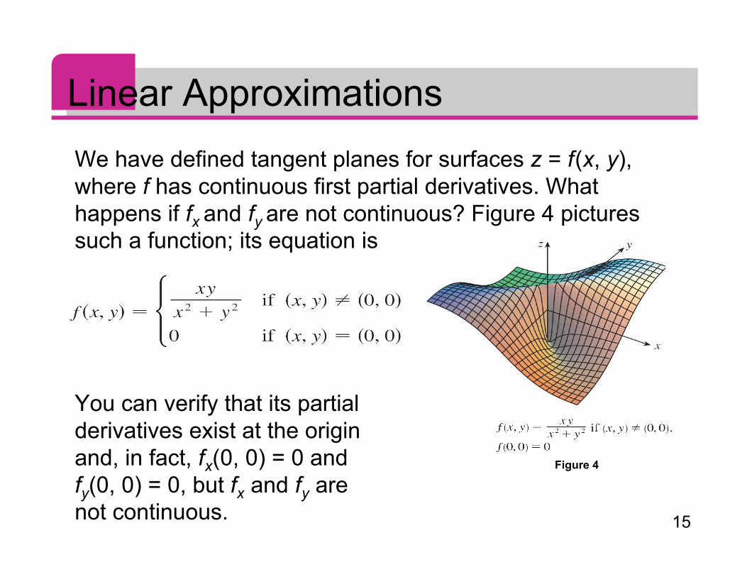
Linear ApproximationsWe have defined tangent planes for surfaces z = f (x, y),where f has continuous first partial derivatives. Whathappens if fx and fy are not continuous? Figure 4 picturessuch a function; its equation is

You can verify that its partialderivatives exist at the originand, in fact, fx(0, 0) = 0 andfy(0, 0) = 0, but fx and fy arenot continuous.

Figure 4

16

Linear ApproximationsThe linear approximation would be f (x, y) ≈ 0, but f (x, y) =at all points on the line y = x.

So a function of two variables can behave badly eventhough both of its partial derivatives exist.

To rule out such behavior, we formulate the idea of adifferentiable function of two variables.

Recall that for a function of one variable, y = f (x), if xchanges from a to a + Δx, we defined the increment of y as

Δy = f (a + Δx) – f (a)

17

Linear Approximations

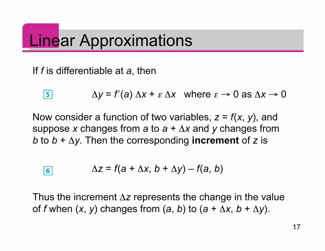
If f is differentiable at a, then

Δy = f ʹ′(a) Δx + ε Δx where ε → 0 as Δx → 0

Now consider a function of two variables, z = f (x, y), andsuppose x changes from a to a + Δx and y changes fromb to b + Δy. Then the corresponding increment of z is

Δz = f (a + Δx, b + Δy) – f (a, b)

Thus the increment Δz represents the change in the valueof f when (x, y) changes from (a, b) to (a + Δx, b + Δy).

18

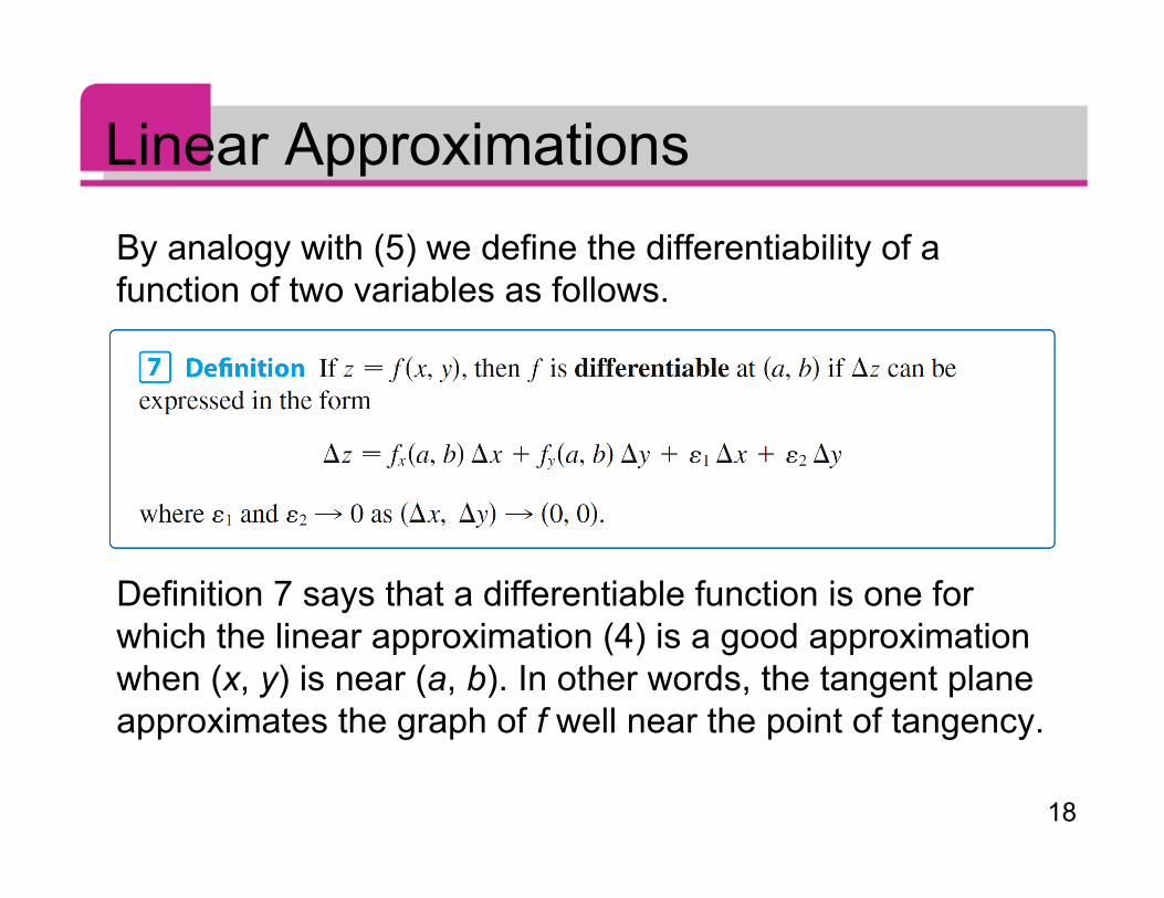
Linear ApproximationsBy analogy with (5) we define the differentiability of afunction of two variables as follows.

Definition 7 says that a differentiable function is one forwhich the linear approximation (4) is a good approximationwhen (x, y) is near (a, b). In other words, the tangent planeapproximates the graph of f well near the point of tangency.

19

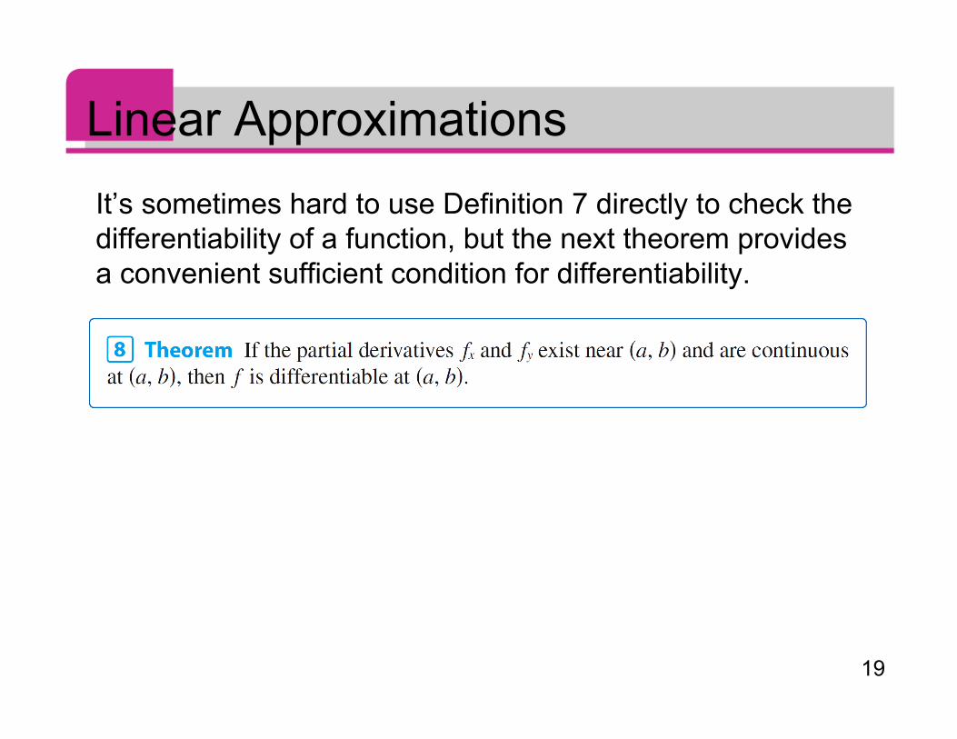
Linear ApproximationsIt’s sometimes hard to use Definition 7 directly to check thedifferentiability of a function, but the next theorem providesa convenient sufficient condition for differentiability.

20

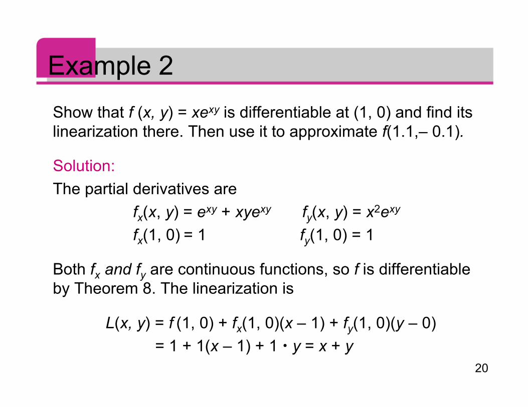
Example 2Show that f (x, y) = xexy is differentiable at (1, 0) and find itslinearization there. Then use it to approximate f(1.1,– 0.1).

Solution:The partial derivatives are fx(x, y) = exy + xyexy fy(x, y) = x2exy

fx(1, 0) = 1 fy(1, 0) = 1

Both fx and fy are continuous functions, so f is differentiableby Theorem 8. The linearization is

L(x, y) = f (1, 0) + fx(1, 0)(x – 1) + fy(1, 0)(y – 0) = 1 + 1(x – 1) + 1 y = x + y

21

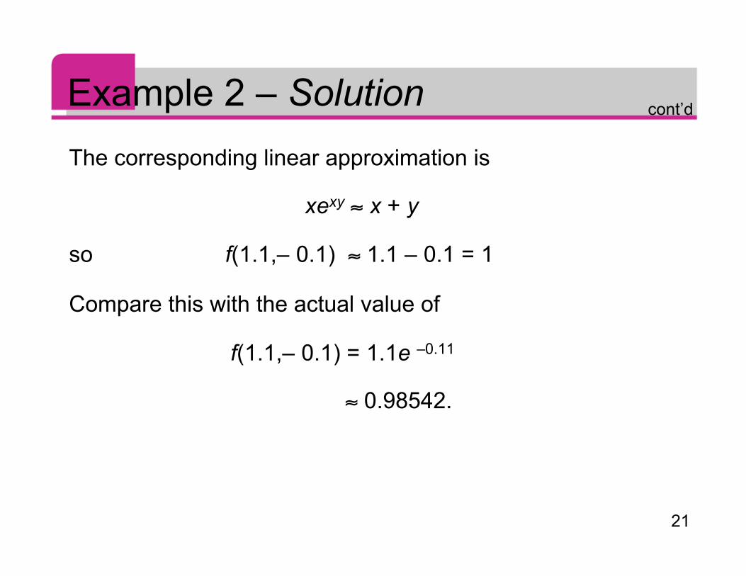
Example 2 – SolutionThe corresponding linear approximation is

xexy ≈ x + y

so f(1.1,– 0.1) ≈ 1.1 – 0.1 = 1

Compare this with the actual value of

f(1.1,– 0.1) = 1.1e –0.11

≈ 0.98542.

cont’d

22

DifferentialsFor a differentiable function of one variable, y = f (x), wedefine the differential dx to be an independent variable; thatis, dx can be given the value of any real number.

The differential of y is then defined as

dy = f ʹ′(x) dx

23

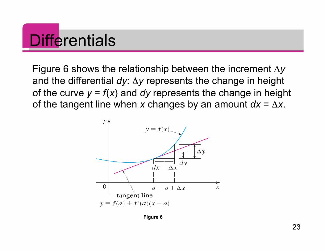
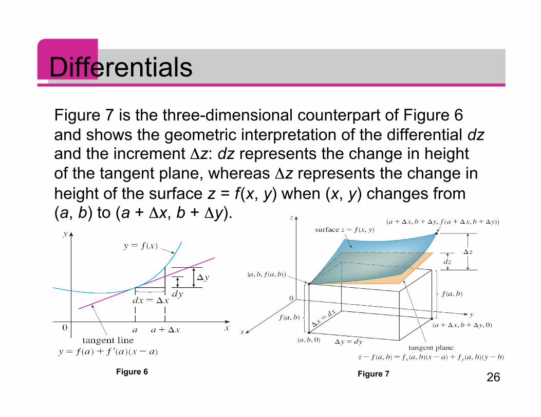
DifferentialsFigure 6 shows the relationship between the increment Δyand the differential dy: Δy represents the change in heightof the curve y = f (x) and dy represents the change in heightof the tangent line when x changes by an amount dx = Δx.

Figure 6

24

DifferentialsFor a differentiable function of two variables, z = f (x, y), wedefine the differentials dx and dy to be independentvariables; that is, they can be given any values. Then thedifferential dz, also called the total differential, isdefined by

Sometimes the notation df is used in place of dz.

25

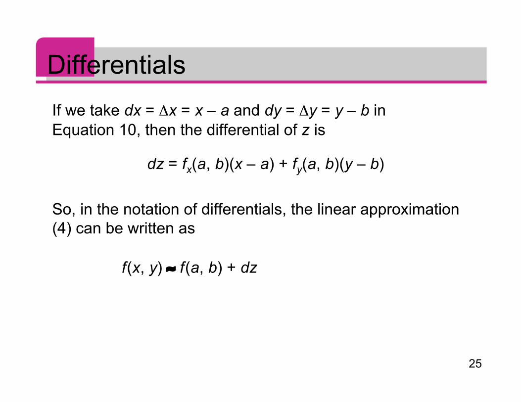
DifferentialsIf we take dx = Δx = x – a and dy = Δy = y – b inEquation 10, then the differential of z is

dz = fx(a, b)(x – a) + fy(a, b)(y – b)

So, in the notation of differentials, the linear approximation(4) can be written as

f (x, y) ≈ f (a, b) + dz

26

DifferentialsFigure 7 is the three-dimensional counterpart of Figure 6and shows the geometric interpretation of the differential dzand the increment Δz: dz represents the change in heightof the tangent plane, whereas Δz represents the change inheight of the surface z = f (x, y) when (x, y) changes from(a, b) to (a + Δx, b + Δy).

Figure 6 Figure 7

27

Example 4(a) If z = f (x, y) = x2 + 3xy – y2, find the differential dz.

(b) If x changes from 2 to 2.05 and y changes from 3 to2.96, compare the values of Δz and dz.

Solution:(a) Definition 10 gives

28

Example 4 – Solution(b) Putting x = 2, dx = Δx = 0.05, y = 3, and dy = Δy = –0.04, we get

dz = [2(2) + 3(3)]0.05 + [3(2) – 2(3)](–0.04)

The increment of z is Δz = f (2.05, 2.96) – f (2, 3) = [(2.05)2 + 3(2.05)(2.96) – (2.96)2]

– [22 + 3(2)(3) – 32] = 0.6449

Notice that Δz ≈ dz but dz is easier to compute.

cont’d

= 0.65

29

Functions of Three or More Variables

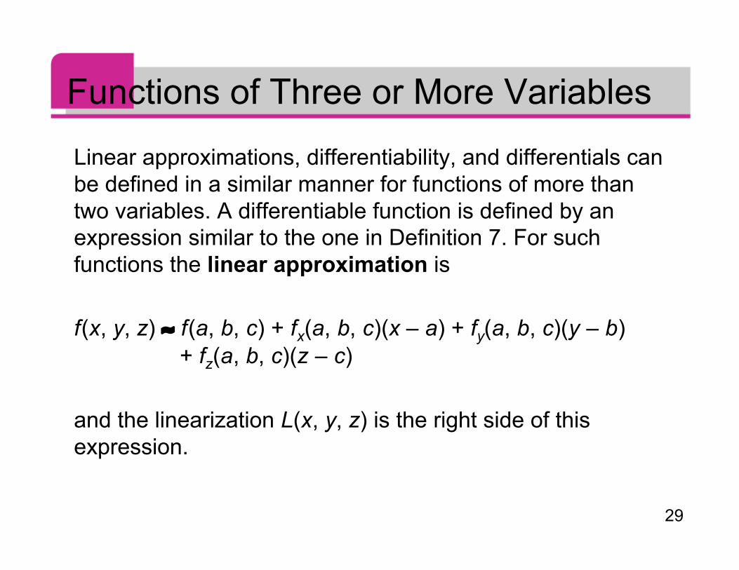
Linear approximations, differentiability, and differentials canbe defined in a similar manner for functions of more thantwo variables. A differentiable function is defined by anexpression similar to the one in Definition 7. For suchfunctions the linear approximation is

f (x, y, z) ≈ f (a, b, c) + fx(a, b, c)(x – a) + fy(a, b, c)(y – b) + fz(a, b, c)(z – c)

and the linearization L(x, y, z) is the right side of thisexpression.

30

Functions of Three or More Variables

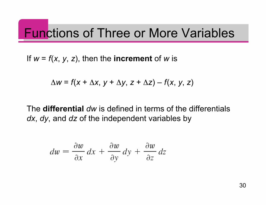
If w = f (x, y, z), then the increment of w is

Δw = f (x + Δx, y + Δy, z + Δz) – f (x, y, z)

The differential dw is defined in terms of the differentialsdx, dy, and dz of the independent variables by

31

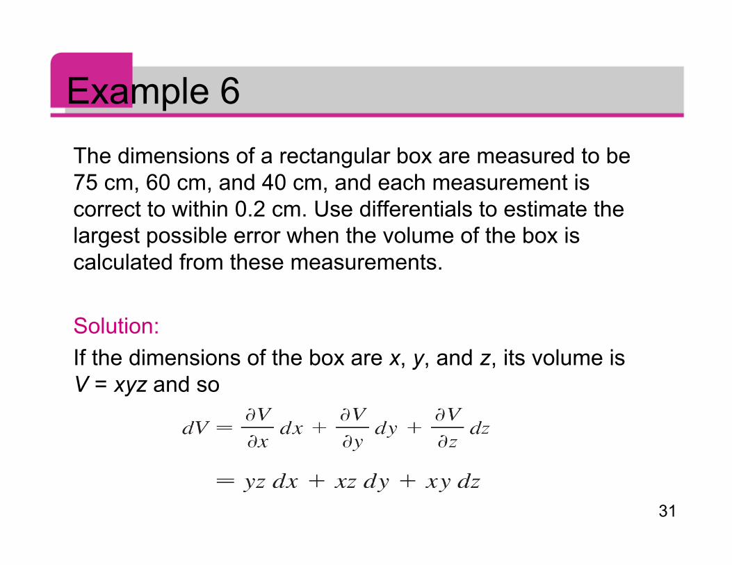
Example 6The dimensions of a rectangular box are measured to be75 cm, 60 cm, and 40 cm, and each measurement iscorrect to within 0.2 cm. Use differentials to estimate thelargest possible error when the volume of the box iscalculated from these measurements.

Solution:If the dimensions of the box are x, y, and z, its volume isV = xyz and so

32

Example 6 – Solution

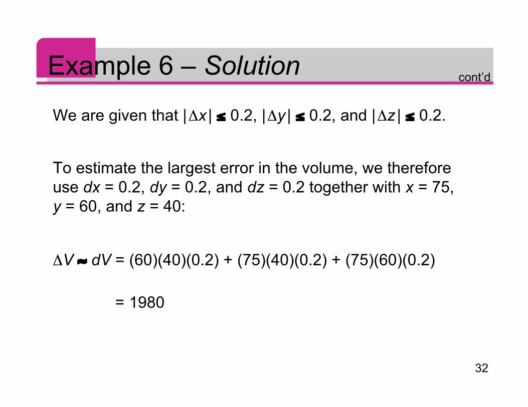
We are given that | Δx | ≤ 0.2, | Δy | ≤ 0.2, and | Δz | ≤ 0.2.

To estimate the largest error in the volume, we thereforeuse dx = 0.2, dy = 0.2, and dz = 0.2 together with x = 75,y = 60, and z = 40:

ΔV ≈ dV = (60)(40)(0.2) + (75)(40)(0.2) + (75)(60)(0.2)

= 1980

cont’d

33

Example 6 – SolutionThus an error of only 0.2 cm in measuring each dimensioncould lead to an error of approximately 1980 cm3 in thecalculated volume! This may seem like a large error, but it’sonly about 1% of the volume of the box.

cont’d