13 Formation of Spectral Lines - Astrophysics Data …ads.harvard.edu/books/1989fsa..book/AbookC13.pdf13 ⋅ Formation of Spectral Lines This choice often causes some grief, for there

II ⋅ Stellar Atmospheres

Copyright (2003) George W. Collins, II

13

Formation of Spectral Lines

. . . Certainly the existence of such striking features as the dark spectral lines that break up the spectra of stars implies the presence of absorption processes that operate in a highly selective manner. The most obvious candidates for this selective absorption are the bound-bound atomic transitions occurring in the abundant species of common elements. Although we saw in Chapter 11 that bound-bound atomic transitions could, when they occur in very large numbers, depress large regions of the spectrum, some transitions will produce lines that dominate the nearby spectrum in a very singular manner. The contrast between these lines and the neighboring spectrum is often so marked that the investigator tends to make a distinction between a specific line and the neighboring spectrum by denoting the spectrum at nearby wavelengths as the "continuum" spectrum.

330

13 ⋅ Formation of Spectral Lines

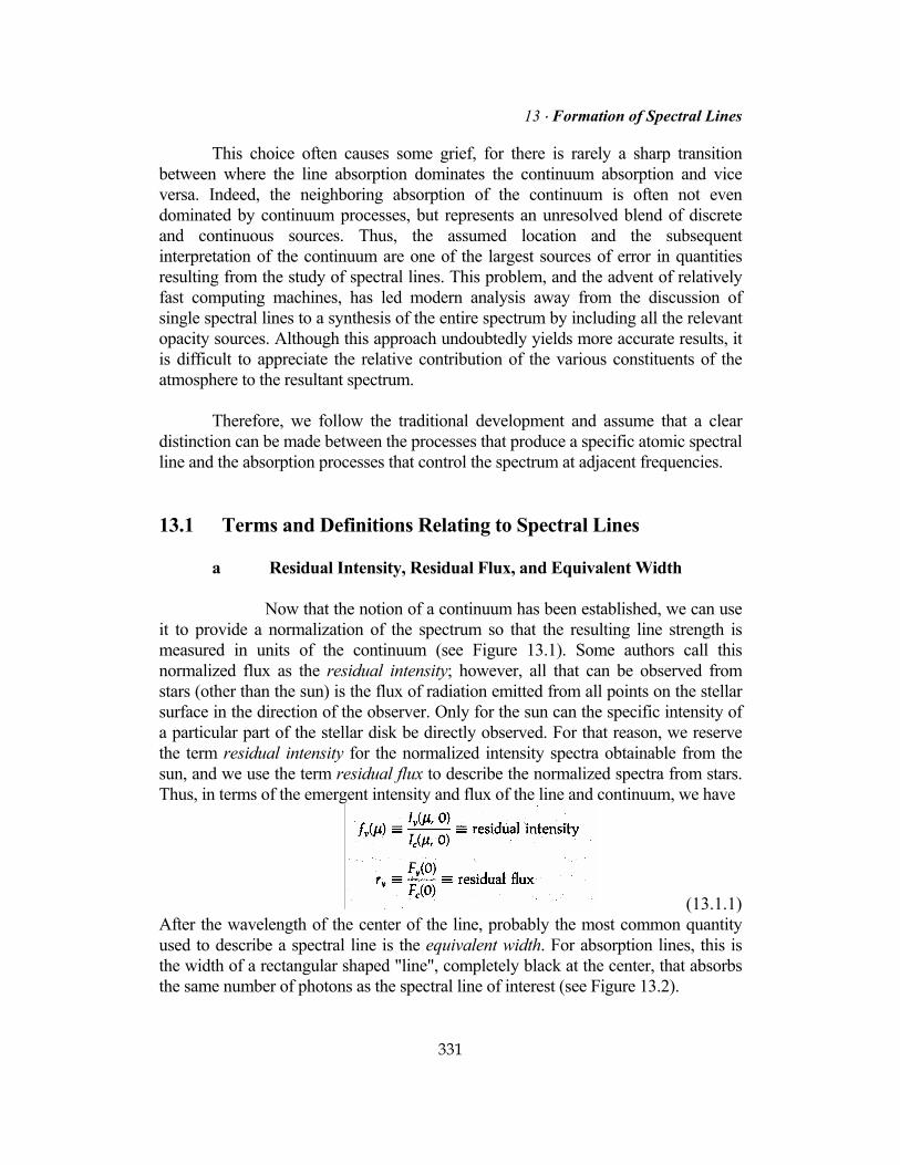
This choice often causes some grief, for there is rarely a sharp transition between where the line absorption dominates the continuum absorption and vice versa. Indeed, the neighboring absorption of the continuum is often not even dominated by continuum processes, but represents an unresolved blend of discrete and continuous sources. Thus, the assumed location and the subsequent interpretation of the continuum are one of the largest sources of error in quantities resulting from the study of spectral lines. This problem, and the advent of relatively fast computing machines, has led modern analysis away from the discussion of single spectral lines to a synthesis of the entire spectrum by including all the relevant opacity sources. Although this approach undoubtedly yields more accurate results, it is difficult to appreciate the relative contribution of the various constituents of the atmosphere to the resultant spectrum. Therefore, we follow the traditional development and assume that a clear distinction can be made between the processes that produce a specific atomic spectral line and the absorption processes that control the spectrum at adjacent frequencies. 13.1 Terms and Definitions Relating to Spectral Lines a Residual Intensity, Residual Flux, and Equivalent Width Now that the notion of a continuum has been established, we can use it to provide a normalization of the spectrum so that the resulting line strength is measured in units of the continuum (see Figure 13.1). Some authors call this normalized flux as the residual intensity; however, all that can be observed from stars (other than the sun) is the flux of radiation emitted from all points on the stellar surface in the direction of the observer. Only for the sun can the specific intensity of a particular part of the stellar disk be directly observed. For that reason, we reserve the term residual intensity for the normalized intensity spectra obtainable from the sun, and we use the term residual flux to describe the normalized spectra from stars. Thus, in terms of the emergent intensity and flux of the line and continuum, we have

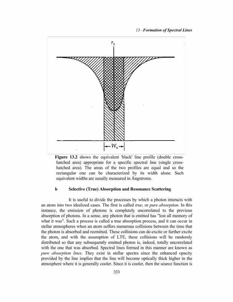
(13.1.1) After the wavelength of the center of the line, probably the most common quantity used to describe a spectral line is the equivalent width. For absorption lines, this is the width of a rectangular shaped "line", completely black at the center, that absorbs the same number of photons as the spectral line of interest (see Figure 13.2).

331


Figure 13.1 shows the shape of a spectral line as it might be observed in units of the absolute flux in the spectrum (panel a). Panel b depicts the same line after normalization by the continuum flux.

We may formally express this definition by

(13.1.2) It is customary to write integrals of this type as ranging from 0 to 4 largely for convenience. What is meant in reality is that the integral should cover those wavelengths for which (1 - rλ) is significantly different from zero. As long as the line is relatively narrow (that is, δλ <<λ0),

(13.1.3)

332


Figure 13.2 shows the equivalent 'black' line profile (double cross-hatched area) appropriate for a specific spectral line (single cross-hatched area). The areas of the two profiles are equal and so the rectangular one can be characterized by its width alone. Such equivalent widths are usually measured in Ångstroms.

b Selective (True) Absorption and Resonance Scattering It is useful to divide the processes by which a photon interacts with an atom into two idealized cases. The first is called true, or pure absorption. In this instance, the emission of photons is completely uncorrelated to the previous absorption of photons. In a sense, any photon that is emitted has "lost all memory of what it was". Such a process is called a true absorption process, and it can occur in stellar atmospheres when an atom suffers numerous collisions between the time that the photon is absorbed and reemitted. These collisions can de-excite or further excite the atom, and with the assumption of LTE, these collisions will be randomly distributed so that any subsequently emitted photon is, indeed, totally uncorrelated with the one that was absorbed. Spectral lines formed in this manner are known as pure absorption lines. They exist in stellar spectra since the enhanced opacity provided by the line implies that the line will become optically thick higher in the atmosphere where it is generally cooler. Since it is cooler, then the source function is

333


smaller and the emergent intensity is less than that of the neighboring continuum. The second type of process is called resonance scattering and it results in the loss of photons in a specialized and indirect manner. Here the photon has a "perfect memory" of its origin. The emitted photon is completely correlated in frequency with the absorbed photon. In Chapter 9, we described such a process as a coherent scattering and lines for which this is true are known as scattering lines. In contrast to the case of pure absorption, a scattering line is formed when the emitted photon is created so soon after the prior absorption that there is no time for the atom to be perturbed by collisions, and the probability of a transition to the prior state is very great. Such cases occur from those states that have very short lifetimes and only one lower level to which the electron can jump. The resonance line transitions meet all these conditions, and hence any resonance line is likely to be a strong scattering line. However, it is possible for any strong line to behave as a scattering line if the probability of returning to the previous state is very large. The same photon that was absorbed is then reemitted, with no net energy exchange with the atom. This is essentially the condition for an interaction to be termed a scattering. The scattering process does not directly result in any loss of energy from the radiation field, but by changing the direction of the photon the process lengthens the stay of the photon in the atmosphere making it subject to destruction by continuum absorption processes. Thus, we can divide spectral lines into two types; the pure absorption lines, where the absorbed energy of the photon is fully shared with the gas, and the resonance scattering lines where it is not. In Chapter 9 we showed that nature is really more complicated than this and in reality most lines can be viewed as a mixture of these two extreme states. However, the radiative transfer of these two kinds of lines is quite different, and understanding the behavior of these two limiting cases will provide a comprehensive basis for understanding the behavior of spectral lines in general. The different behavior of these two processes is clearly seen by noting that the energy of a pure absorption process is shared immediately with the gas while that of a resonance scattering processes is not. Scattering is a fully conservative process and therefore cannot, by itself, result in the destruction of photons. However, scattering does change the direction of a photon, thereby increasing the distance that the photon must travel through the atmosphere before escaping into interstellar space. Any process that lengthens the path of a photon through the atmosphere also enhances the probability that the photon will be absorbed by some other process such as continuum absorption. Thus, the redirection of line photons that results from resonant scattering also produces a net loss of these photons relative to those in the neighboring continuum. This, then, is the origin of the resonance scattering lines in stellar spectra.

334


c Equation of Radiative Transfer for Spectral Line Radiation It is customary to denote the part of the mass extinction coefficient that results from pure absorption processes by the letter κ, while the part that results from scattering is represented by the Greek letter σ. Those photon interactions that occur as a result of absorptions within the line are subscripted by the letter ν. Since the continuum processes generally vary quite slowly across a spectral line, we omit the subscript ν entirely. Thus,

(13.1.4) Since the origin of the equation of radiative transfer was dealt with extensively in Section 9.2, we provide only a brief derivation here. Basically we balance the energy passing in and out of a differential volume along a specific path through the atmosphere. If we do this for a plane-parallel atmosphere where we keep the line and continuum processes separate, we get

(13.1.5) where the first term on the right-hand side represents the energy lost from the beam. The second and third terms on the right-hand side denote the contributions to the beam within the differential volume. The first of these is just due to thermal emission, while the second results from scattering by both line and continuum processes. By making the usual identification between the Planck function and the processes of thermal emission and absorption, the equation of radiative transfer for line radiation becomes

(13.1.6) where the optical depth in the line τν is given by

(13.1.7)

335


13.2 Transfer of Line Radiation through the Atmosphere Calculating a stellar spectral line is rather simpler than constructing a model stellar atmosphere since the structure of the atmosphere can be assumed to be known. We need only bring those methods discussed in Chapter 10 for the solution of the equation of transfer to bear on the solution of equation (13.1.6). However, to obtain the line profile, we also have to solve the same equation with κν = σν = 0 so that we may determine the continuum flux with which to normalize the line profile. Although this procedure will indeed work and is in fact used for most modern line profile calculations, it is very difficult to obtain any insight into the behavior of scattering and absorption lines from the numerical output. However, their behavior can be seen in some older semi-analytic solutions to simple models of line transfer. a Schuster-Schwarzschild Model Atmosphere for Scattering Lines The Schuster-Schwarzschild model atmosphere is perhaps the simplest model that one can suggest for line formation. It is to spectral line transfer theory what the gray atmosphere is to atmosphere theory. The model is basically appropriate for strong resonance lines which are formed in a thin layer overlying the photosphere (see Figure 13.3). If the lines of interest are quite strong, then the opacity in the continuum is negligible compared to the line opacity. Furthermore, since the process of scattering is fully conservative and the photons do not exchange energy with the local constituents of the atmosphere, we need not worry about the physical conditions in the cool gas that overlies the photosphere. Just as with the gray atmosphere, pure scattering decouples the radiation field from the physics of the gas. We further assume that the optical depth in the line corresponding to the location of the photosphere is finite. The plane-parallel equation of radiative transfer appropriate for this model can be obtained from equation (13.1.6) by specifying the values for the absorption and scattering coefficients. Thus,

(13.2.1) where

(13.2.2) Since the line extinction coefficient is entirely due to scattering, it is not surprising that equation (13.2.1) looks like the transfer equation for the gray atmosphere [equation (10.2.1)]. This means that radiative equilibrium requires the flux to be constant at each frequency throughout the line. To be sure, the constant

336


will be different for each frequency, but the flux at any particular frequency will not vary with the depth. The condition of monochromatic flux constancy can be expressed as

(13.2.3)

Figure 13.3 shows a schematic representation of the Schuster-Schwarzschild Model Atmosphere for the formation of strong scattering lines.

Solution of the Radiative Transfer Equation for the Schuster-Schwarzschild Model Since the equation of transfer for line radiation in this model formally resembles the gray atmosphere equation; we may use the results of Chapter 10 to find the solution. Specifically, equation (10.2.31) gives a general result for the solution of the plane-parallel finite gray atmosphere. However, to keep the discussion simple, we take n = 2. Then the appropriate zeros of the Legendre polynomials require that

31±=iµ and equation (10.2.31) becomes

(13.2.4) where the subscripts '+' and '-' refer to the outward- and inward-directed streams of radiation, respectively. Applying the surface boundary condition that I_ (0) = 0 we find

(13.2.5) and the complete solution becomes

337


(13.2.6) This solution for the gray atmosphere is sometimes called the Chandrasekhar two-stream approximation. It conceptually replaces the entire radiation field by two streams of radiation directed along a line oriented about 54 degrees ( 3

1±=iµ ) to the normal of the atmosphere. The result is nearly identical to that obtained from the Eddington approximation, only the angle is slightly different. Residual Flux and Intensity for the Schuster-Schwarzschild Model The ratio of the emergent flux in the line to that of the continuum can be obtained immediately by requiring that the line intensity incident on the base of the cool gas be the same as the emergent intensity in the neighboring continuum, so that

(13.2.7) Here τ0 is the optical depth at any frequency in the line measured at the base of the atmosphere. This value is zero for all frequencies corresponding to the continuum. The quantity Fc is just the continuum flux. Thus, the residual flux is

(13.2.8) However, to complete the description of the Schuster-Schwarzschild model, we would like an expression for the residual intensity fν. To obtain the angle dependence of the intensity we have to appeal to the classical solution of the equation of transfer for a finite atmosphere, so that the emergent intensity is

(13.2.9) The value for the mean intensity Jν(τν) can be obtained directly from the two-stream approximation as

(13.2.10) Substitution of this into equation (13.2.9) and then into the definition for the residual intensity [equation (13.1.1)] yields

(13.2.11) Remember that t0 is a function of frequency, and so its behavior with frequency will determine the line shape or profile. 338


To see how scattering lines will vary in strength across the surface of a stellar disk, consider some limiting cases.

(13.2.12) The first of equations (13.2.12) represents relatively weak spectral lines (or the wings of strong lines). Here there is no angular dependence whatsoever except that dictated by the limb-darkening of the continuum. Thus, we can expect that even weak scattering lines will be visible at all points on the stellar disk with equal strength. While the strong lines described by the second of equations (13.2.12) do show some limb-darkening through the dependence on µ, that dependence is not great. The range in line strength to be expected for a strong scattering line between one formed near the center of the disk and one formed at the limb is about a factor of 2. As we see, this contrasts greatly with the behavior of spectral lines formed by pure absorption processes. However, a model that includes absorption processes must include information about the atmospheric structure and so will be somewhat more sophisticated. One such model atmosphere is known as the Milne-Eddington model. b Milne-Eddington Model Atmosphere for the Formation of

Spectral Lines To appreciate the importance of pure absorption in the formation of a spectral line, we must acknowledge the fact that pure absorption processes imply an interaction between the radiation field and the particles that make up the gas. Thus, we will have to specify something about the behavior of the opacity and source function with optical depth. The trick is to place as few limitations as possible so as to preserve generality and to make those limitations "reasonable" and yet specify the situation sufficiently to guarantee a unique solution. The Milne-Eddington model is considerably more sophisticated than the Schuster-Schwarzschild model and is correspondingly more complicated. It attempts to simultaneously include the effects of absorption and scattering in the line extinction coefficient (that is, κν+σν). Let us define the following parameters in terms of the absorption and scattering coefficients of the line and continuum:

339


(13.2.13) The parameter εν measures the relative importance of pure absorption to total extinction for processes involving the spectral line, and ην is a measure of the line strength, since it is a ratio of the total line extinction coefficient to that of the continuum. The Milne-Eddington model does make the somewhat restrictive assumption that scattering processes are relatively unimportant for continuum photons. Hence, σ = 0. The parameter ℒ is clearly not linearly independent of εν and ην, but is useful to introduce because it measures the relative importance of total absorption to total extinction for all processes of the line and continuum that operate on the photons passing through the atmosphere. By substituting these values into the equation for the transfer of line radiation [equation (13.1.6)], we have the appropriate equation of transfer for the Milne-Eddington model atmosphere

(13.2.14) A simpler equation of transfer for the continuum radiation can be obtained simply by letting κν and σν go to zero, so that

(13.2.15) Now if we relate the structure of the atmosphere to the source function in the line through its behavior in the continuum, we can write

(13.2.16) Here, we have made use of the Eddington approximation where the asymptotic behavior of the source function with optical depth is linear [see equation (10.2.32)]. To find the behavior of the residual intensity and flux for the line, we follow basically the same steps as for the Schuster-Schwarzschild model. Solution of the Equation of Radiative Transfer for the Milne-Eddington Model Atmosphere Before we can solve equations (13.2.14), we must make one additional assumption regarding the behavior of the opacity coefficients with atmospheric depth. We assume that both εν and ην (and hence ℒν) are not functions of depth in the atmosphere and can therefore be regarded as constants in the equation

340


of transfer [equations (13.2.14)]. While it is certainly unreasonable to expect that any of the absorption or scattering coefficients are independent of depth, since they depend strongly on temperature, it is not unreasonable to think that their ratios may be approximately constant. If we now solve equation (13.2.14) by taking moments of the equation, we obtain

(13.2.17) Using that part of the Eddington approximation that says Kν . Jν/3 and differentiating the second of equations (13.2.17), we get

(13.2.18) Now we can relate Bν(t) to the optical depth in the line by noting that

(13.2.19) so that

(13.2.20) This allows us to write

(13.2.21) Substitution of this depth dependence of the Planck function admits a solution of equation (13.2.18) of the form

(13.2.22) where the constants c1 and c2 are to be determined from the boundary conditions. Unlike the Schuster-Schwarzschild model atmosphere, the Milne-Eddington model is a semi-infinite atmosphere so that at large depths we may be assured that Jν → Bν which requires c1 = 0. To determine c2, we apply the part of the Eddington approximation that we have not used [that is, Jν(0) = ½Fν(0)]. This can be combined with the assumption about Kν to determine a value for the derivative of Jν at the surface, namely,

341


(13.2.23) The right-hand side of this result is obtained from the solution [equation (13.2.22)] itself. If we differentiate that solution and evaluate the result at the surface, we have

(13.2.24) which yields the following value of c2:

(13.2.25) Had we used the Chandrasekhar two-stream approximation to solve the equation of transfer, we would have gotten

(13.2.26) This indicates that the solution is not too sensitive to the mode of solution of the equation of transfer. Residual Flux and Intensity for the Milne-Eddington Model The residual flux can be obtained from its definition and the Eddington approximation so that

(13.2.27) In the continuum, ην = 0 and ℒν = 1 so that

(13.2.28) This leads to a residual flux given by

3.2.29) To evaluate the residual intensity, we must again use the classical solution to the equation of transfer. However, to do so, we must have expressions for the source function in the line and continuum. It is clear from the equation of transfer [equation (13.2.14)] that the line source function is

342 (13.2.30)


Again, remembering that in the continuum ℒν = 1 , we see that the source function for the continuum is just

(13.2.31) Substitution of these two source functions into the classical solution for the equation of transfer, and some algebra, gives the residual intensity as

(13.2.32) Some aspects of this solution should not surprise us. For example, the term a+bµ is simply 1/µ times the Laplace transform of the continuum source function a+bt. Similarly, the numerator of the first term is the Laplace transform of the Planck fnction in the line, so that the lead term of equation (13.2.32) is just the ratio of the Laplace transforms of the absorption components of the line to the continuum source functions. This is to be expected from the result obtained for limb-darkening in Chapter 10 [equations (10.1.19), and (10.1.20)]. Since the second term vanishes for the case of pure absorption (that is, ℒ → 1), this term must represent the contribution of scattering in the line to the residual intensity. Asymptotic Behavior of the Residual Flux and Intensity Because of the increased generality of the Milne-Eddington model over the Schuster-Schwarzschild model, we can investigate the asymptotic behavior of the line not only with strength but also as the line extinction coefficient ranges from pure absorption to pure scattering. In the case of pure absorption εν = 1, ℒν = 1 and equations (13.2.29) and (13.2.32) become

(13.2.33) Note that in an isothermal atmosphere (that is, b = 0) both the residual intensity and the flux are asymptotic to unity and the line disappears. Thus, as one might expect, if there are no temperature gradients, there can be no spectral absorption lines. The radiation field would then be in STE and the source function as well as the radiation field would be given by the Planck function regardless of the dependence of the absorption coefficient on frequency. For stellar atmospheres, this has the more immediate implication that the stronger the source function gradient the stronger the line. This is the simple explanation of why the central depths of the lines in late-type stars are so much darker than those for the early-type stars. For the later type stars, the visible part of the spectrum tends to lie at wavelengths shorter than that of the stellar energy maximum. For these wavelengths, the source function varies as a large power of the

343


temperature so that the stellar temperature gradient produces a very steep source function gradient. For the early-type stars, the visible part of the spectrum lies well to the red end of the energy maximum on what is generally called the Rayleigh-Jeans tail of the energy distribution. Here the source function varies quite slowly so that the temperature gradient produces a gentler source function gradient and weaker absorption lines. If we investigate the case for strong absorption lines, we have

(13.2.34) and as one expects, the above results hold if b = 0. However, in a normal stellar atmosphere where b ≠ 0 even the strongest line must vanish as µ → 0 at the limb. Thus we expect that the pure absorption component of the line extinction coefficient will play no role in determining the line strength at the limb of the star. This is easier to understand if we consider the physical situation encountered at the limb. The observer's line of sight just grazes the atmosphere passing through a region of reasonably constant conditions including the temperature. Thus, there are no temperature or source function gradients along the line of sight. If no photons are scattered from other locations into the line of sight, then the only contribution to the observed intensity comes from a nearly isothermal sight line through the atmosphere. If there are no gradients, there are no pure absorption lines. In the event that ην << 1, which prevails for weak absorption lines, the residual flux and intensity are given by

(13.2.35) As one might expect, the line strength is simply proportional to ην, which is proportional to κν which in turn is proportional to the number abundance of absorbers. Hence for weak lines we expect that the strength of the line would primarily depend on the abundance of the element giving rise to the line.

In the case of pure scattering, εν=0, which requires that

(13.2.36) For the situation where ην >> 1 and we have very strong scattering lines, the residual flux and intensity become

344


(13.2.37) Even in the event that the atmosphere is isothermal, scattering lines will persist. Indeed, even at the limb of an isothermal atmosphere, the residual intensity is still of the order of one-half of the residual flux which nicely illustrates the ubiquitous property of scattering lines. The physical reason for this is that these lines do not depend on the thermodynamic properties of the gas for their existence. The lines result from the existence of a boundary or a surface to the atmosphere. If there were no surface, then again conditions of STE would prevail and there would be no lines of any kind. However, the presence of a boundary permits the selective escape of photons. Those that are heavily scattered will wander about in the atmosphere for a greater time than those photons that do not experience scattering. Hence, the likelihood that the photons will be absorbed by continuum processes and thereby removed from the beam is increased. This will happen in an isothermal atmosphere as well as in a normal atmosphere. Thus, scattering lines will always be present in a stellar spectrum. For the case of weak scattering lines, ην = 1,and ℒν = 1 causing the residual flux and intensity to take the form

(13.2.38) for ην<<1. Under these conditions, the residual flux takes on the form of the result for the case of weak pure absorption. However, even in this case the limb-darkening behavior of the line as given by fν is different from the corresponding expression [equation (13.2.35)] for weak absorption. Even at the limb of an isothermal atmosphere a weak scattering line will be visible. The main purpose of studying these approximate atmospheres is to gain some feeling for the manner in which line strengths vary and to see which parameters are most instrumental in determining the extent of that variation. Lines formed under the conditions of pure absorption behave in a qualitatively different manner from lines where the extinction coefficient is dominated by scattering. You must keep this idea clearly in mind whenever you wish to relate an observed line strength or shape to a theoretically determined model. You must do the radiative transfer correctly.

345


Knowledge of the behavior of spectral lines also will serve you well when you try to understand the results of a complex model atmosphere computer code. If the line does not behave in a manner described by these simple models, then there must be a good and compelling reason that should be understood by the investigator. Although the 1940s and 1050s generated additional approaches to the problem of radiative transfer of line radiation, most of that work has been superceded by the advent of high-speed computers and large complex atmosphere codes. The contemporary approach basically treats the line absorption coefficient as an additional opacity source that has a strongly variable frequency dependence. Thus, no special distinction is made between opacity due to lines and that of the continuum. The problem of locating the continuum for the purposes of generating a line profile is then about the same for the model maker as for the observer. The many complex physical processes that contribute to the shape of the line, and whose importance varies with position in the atmosphere, are automatically included in the calculations. However, for obtaining insight into the processes of line formation, these simple models remain most useful. Problems 1. Find equivalent expressions for the asymptotic behavior of the residual

intensity and flux as given by equations (13.2.33) through (13.2.37) for the case where the radiative transfer equation is solved by the Chandrasekhar two-stream approximation.

2. Find expressions for the residual intensity and flux of a Schuster-

Schwarzschild atmosphere if the equation of transfer is to be solved by using the Chandrasekhar nth-order approximation.

3. Show that the expression for fν can be used to obtain the expression for rν for the Milne-Eddington atmosphere.

4. Find an expression for rν in a Milne-Eddington atmosphere where the source function in the continuum is given by

5. Derive expressions for a Milne-Eddington type of model atmosphere of finite

optical depth τ0 for fν(µ) and rν. Assume the atmosphere is illuminated from below by a uniform isotropic intensity I0.

346


347

6. Compare the results of Problem 5 to the results obtained for a the semi-infinite Milne-Eddington atmosphere for strong absorption lines and strong scattering lines and b the Schuster-Schwarzschild atmosphere for strong scattering lines and weak scattering lines. 7. If the law of limb-darkening for lines formed in a Schuster-Schwarzschild atmosphere can be written as

find a and b in terms of the continuum flux and the optical depth of the line τ0.

8. Find an expression for the residual flux from a Schuster-Schwarzschild atmosphere if the continuum photospheric intensity has the form

9. Use a model atmosphere code to generate rν for the spectral line of your choice, and compare the results to those of a Milne-Eddington atmosphere with the same effective temperature. Clearly state all assumptions and approximations that you make.

Supplemental Reading A reasonable derivation of the solution of the equation of radiative transfer for the Milne-Eddington model atmosphere can be found in

Aller, L. H.: The Atmospheres of the Sun and Stars, 2d ed. Ronald, New York, 1963, pp.349 - 352

An excellent general reference for the formation of spectral lines is: Jefferies, J. T.: Spectral Line Formation, Blaisdell, Waltham, Mass., 1968. In particular, Jefferies discusses the Schuster-Schwarzschild atmosphere in Section 3.2 p.30. A quite complete discussion of classical line transport theory can be found in these two books:

Mihalas, D.: Stellar Atmospheres, 2d ed., W.H.Freeman, San Francisco, 1978, pp. 308 - 316. Mihalas, D.: Stellar Atmospheres, W.H.Freeman, San Francisco, 1970, pp.323 - 332.

Documents

13 Formation of Spectral Lines - Astrophysics Data …ads.harvard.edu/books/1989fsa..book/AbookC13.pdf13 ⋅ Formation of Spectral Lines This choice often causes some grief, for there