8 - Stellar Pulsation and Oscillationads.harvard.edu/books/1989fsa..book/AbookC08.pdf · 2003-01-29 · 8 ⋅ Stellar Pulsation and Oscillation (8.1.12) Substitution of this form

8 ⋅ Stellar Pulsation and Oscillation

Copyright (2003) George W. Collins, II

8

Stellar Pulsation and Oscillation

. . .

201

That some stars vary in brightness has been known from time immemorial. That this variation is the result of intrinsic changes in the star itself has been known for less than 100 years and the causes of those variations have been understood for less than 30 years. It is not a simple matter to distinguish the light variations resulting from eclipses by a companion from those caused by physical changes in the star itself. However, for the cepheid variables (named for the prototype example δ Cepheii), the treatment of the light variations as if they resulted from eclipses by a companion leads to some absurd results. If this were the case, the orbit of the companion would have to be highly elliptical with the semimajor axes pointed toward the earth. This somewhat Ptolemaic view suggests that the binary hypothesis is incorrect but is far from conclusive. Further analysis shows that the sum of the radii for the two hypothetical stars would exceed their separation. Such a situation is even less likely. However, the coup degrace is administered to the binary hypothesis when one considers the radial velocity curve produced by the star throughout a period of light variation. Here one finds that maximum radial velocity occurs near minimum light, which is nearly the reverse of that required by the binary hypothesis. Thus, one is left with almost no other option than to conclude that this class of stars is intrinsically varying.

1 ⋅ Stellar Interiors

While a number of other types of stars were seen to exhibit similar behavior, considerable interest was generated by the Cepheid variables themselves when it was found that a relationship exists between the period of variability and the absolute luminosity at maximum brightness. This period-luminosity relationship was found to hold true, in one form or another, for the intrinsic variables. While it is true that the RR Lyrae stars have basically the same absolute magnitude regardless of their period, this can be viewed as a period luminosity relation since the very determination of the RR Lyrae nature of a star establishes its luminosity. Thus, variable stars could be used as "standard candles" for the purposes of distance determination. Although it is not necessary to understand the physical processes giving rise to the variation of light in these stars to use them to determine distances to associated objects, the lack of such understanding may result in large errors of interpretation. Such was the case with the Cepheid variables, and the result was an error in the distances to galaxies of about a factor of 2. Although this error was uncovered before the nature of stellar pulsation was understood, there can be little doubt that such an understanding would have signaled the danger much earlier and possibly prevented much confusion. The detailed nature of the origin of pulsation for the intrinsic variables was not understood until the computational power existed for the accurate construction of model stars. Then, for the two most important classes of intrinsic variables, it was found that the mechanism producing the light variations resulted from oscillations in the ionization equilibrium in the outer layers of the star and had nothing to do with oscillations in the energy generation process itself. However, in order to construct these models, it is necessary to have some idea about the nature of the stars themselves. Here their variations provide the clues required. From the stability of the periods of these pulsating stars, it is clear that the oscillations are resonant oscillations, and their periods will tell us much about the stars involved. We have already established the conceptual foundation for this determination in the Virial theorem. 8.1 Linear Adiabatic Radial Oscillations Just as the pitch or oscillation frequency of an orchestral chime conveys information about its length, so the oscillation period of a pulsating variable should indicate its size. The low-pitch, or long- period, chimes or bells are characteristically larger than higher-pitch ones. So it is with the most common of the pulsating stars. The RR Lyrae stars having pulsational periods of less than a day are both hotter and less luminous, and therefore smaller, than the longer-period Cepheid variables. The Cepheid variables in turn are significantly hotter and smaller than the even longer period Mira variables. Only for the cataclysmic variables, where the pulsations are probably mediated by an outside source, does this size-period relationship fail. This is as it should be, for the pulsation of a star, being a hydrodynamic phenomenon, 202


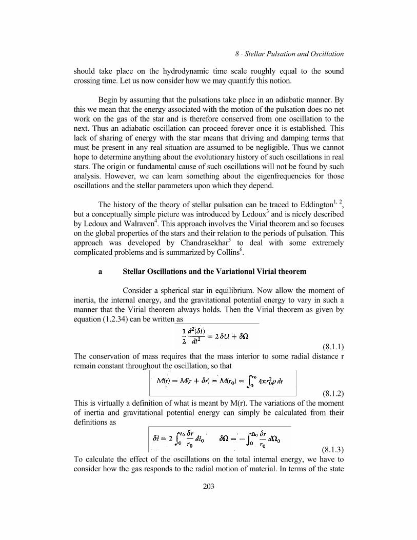
should take place on the hydrodynamic time scale roughly equal to the sound crossing time. Let us now consider how we may quantify this notion. Begin by assuming that the pulsations take place in an adiabatic manner. By this we mean that the energy associated with the motion of the pulsation does no net work on the gas of the star and is therefore conserved from one oscillation to the next. Thus an adiabatic oscillation can proceed forever once it is established. This lack of sharing of energy with the star means that driving and damping terms that must be present in any real situation are assumed to be negligible. Thus we cannot hope to determine anything about the evolutionary history of such oscillations in real stars. The origin or fundamental cause of such oscillations will not be found by such analysis. However, we can learn something about the eigenfrequencies for those oscillations and the stellar parameters upon which they depend. The history of the theory of stellar pulsation can be traced to Eddington1, 2, but a conceptually simple picture was introduced by Ledoux3 and is nicely described by Ledoux and Walraven4. This approach involves the Virial theorem and so focuses on the global properties of the stars and their relation to the periods of pulsation. This approach was developed by Chandrasekhar5 to deal with some extremely complicated problems and is summarized by Collins6. a Stellar Oscillations and the Variational Virial theorem Consider a spherical star in equilibrium. Now allow the moment of inertia, the internal energy, and the gravitational potential energy to vary in such a manner that the Virial theorem always holds. Then the Virial theorem as given by equation (1.2.34) can be written as

(8.1.1) The conservation of mass requires that the mass interior to some radial distance r remain constant throughout the oscillation, so that

(8.1.2) This is virtually a definition of what is meant by M(r). The variations of the moment of inertia and gravitational potential energy can simply be calculated from their definitions as

(8.1.3) To calculate the effect of the oscillations on the total internal energy, we have to consider how the gas responds to the radial motion of material. In terms of the state

203


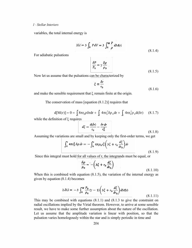
variables, the total internal energy is

(8.1.4) For adiabatic pulsations

(8.1.5) Now let us assume that the pulsations can be characterized by

(8.1.6) and make the sensible requirement that ξ remain finite at the origin. The conservation of mass [equation (8.1.2)] requires that

∫ ∫ ∫ δρπ+δρπ+ρδπ==r

0

r

0

r

0 0200

200 )r(dr4drr4rdrr80)]r(M[d (8.1.7)

while the definition of ξ requires

(8.1.8) Assuming the variations are small and by keeping only the first-order terms, we get

(8.1.9) Since this integral must hold for all values of r, the integrands must be equal, or

(8.1.10) When this is combined with equation (8.1.5), the variation of the internal energy as given by equation (8.1.4) becomes

(8.1.11) This may be combined with equations (8.1.1) and (8.1.3 to give the constraint on radial oscillations implied by the Virial theorem. However, to arrive at some sensible result, we have to make some further assumption about the nature of the oscillation. Let us assume that the amplitude variation is linear with position, so that the pulsation varies homologously within the star and is simply periodic in time and 204


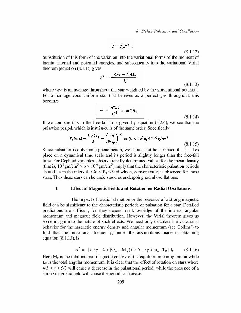
(8.1.12) Substitution of this form of the variation into the variational forms of the moment of inertia, internal and potential energies, and subsequently into the variational Virial theorem [equation (8.1.1)] gives

(8.1.13) where <γ> is an average throughout the star weighted by the gravitational potential. For a homogeneous uniform star that behaves as a perfect gas throughout, this becomes

(8.1.14) If we compare this to the free-fall time given by equation (3.2.6), we see that the pulsation period, which is just 2π/σ, is of the same order. Specifically

(8.1.15) Since pulsation is a dynamic phenomenon, we should not be surprised that it takes place on a dynamical time scale and its period is slightly longer than the free-fall time. For Cepheid variables, observationally determined values for the mean density (that is, 10-3gm/cm3 > p > 10-6 gm/cm3) imply that the characteristic pulsation periods should lie in the interval 0.3d < Pp < 90d which, conveniently, is observed for these stars. Thus these stars can be understood as undergoing radial oscillations.

b Effect of Magnetic Fields and Rotation on Radial Oscillations The impact of rotational motion or the presence of a strong magnetic field can be significant to the characteristic periods of pulsation for a star. Detailed predictions are difficult, for they depend on knowledge of the internal angular momentum and magnetic field distribution. However, the Virial theorem gives us some insight into the nature of such effects. We need only calculate the variational behavior for the magnetic energy density and angular momentum (see Collins6) to find that the pulsational frequency, under the assumptions made in obtaining equation (8.1.13), is

0002 35)M(43[ ω>γ−<+−Ω>−γ<−=σ L0 ]/I0 (8.1.16)

Here M0 is the total internal magnetic energy of the equilibrium configuration while L0 is the total angular momentum. It is clear that the effect of rotation on stars where 4/3 < γ < 5/3 will cause a decrease in the pulsational period, while the presence of a strong magnetic field will cause the period to increase.

205


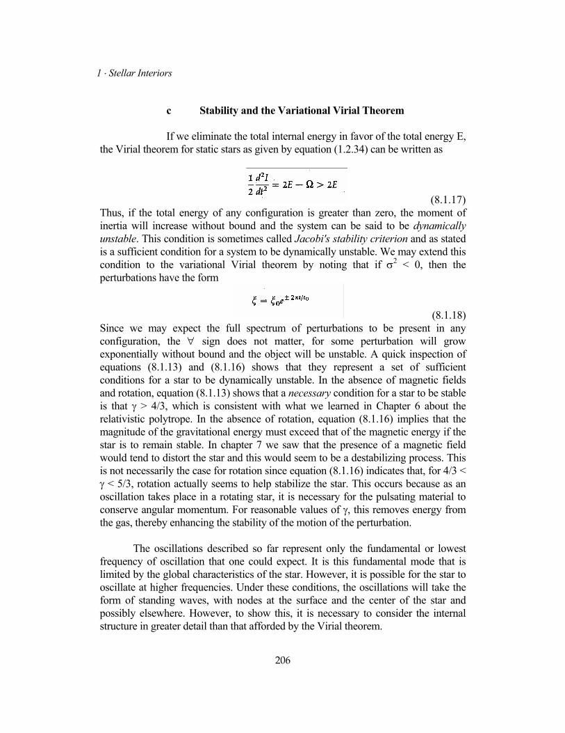
c Stability and the Variational Virial Theorem If we eliminate the total internal energy in favor of the total energy E, the Virial theorem for static stars as given by equation (1.2.34) can be written as

(8.1.17) Thus, if the total energy of any configuration is greater than zero, the moment of inertia will increase without bound and the system can be said to be dynamically unstable. This condition is sometimes called Jacobi's stability criterion and as stated is a sufficient condition for a system to be dynamically unstable. We may extend this condition to the variational Virial theorem by noting that if σ2 < 0, then the perturbations have the form

(8.1.18) Since we may expect the full spectrum of perturbations to be present in any configuration, the ∀ sign does not matter, for some perturbation will grow exponentially without bound and the object will be unstable. A quick inspection of equations (8.1.13) and (8.1.16) shows that they represent a set of sufficient conditions for a star to be dynamically unstable. In the absence of magnetic fields and rotation, equation (8.1.13) shows that a necessary condition for a star to be stable is that γ > 4/3, which is consistent with what we learned in Chapter 6 about the relativistic polytrope. In the absence of rotation, equation (8.1.16) implies that the magnitude of the gravitational energy must exceed that of the magnetic energy if the star is to remain stable. In chapter 7 we saw that the presence of a magnetic field would tend to distort the star and this would seem to be a destabilizing process. This is not necessarily the case for rotation since equation (8.1.16) indicates that, for 4/3 < γ < 5/3, rotation actually seems to help stabilize the star. This occurs because as an oscillation takes place in a rotating star, it is necessary for the pulsating material to conserve angular momentum. For reasonable values of γ, this removes energy from the gas, thereby enhancing the stability of the motion of the perturbation. The oscillations described so far represent only the fundamental or lowest frequency of oscillation that one could expect. It is this fundamental mode that is limited by the global characteristics of the star. However, it is possible for the star to oscillate at higher frequencies. Under these conditions, the oscillations will take the form of standing waves, with nodes at the surface and the center of the star and possibly elsewhere. However, to show this, it is necessary to consider the internal structure in greater detail than that afforded by the Virial theorem.

206


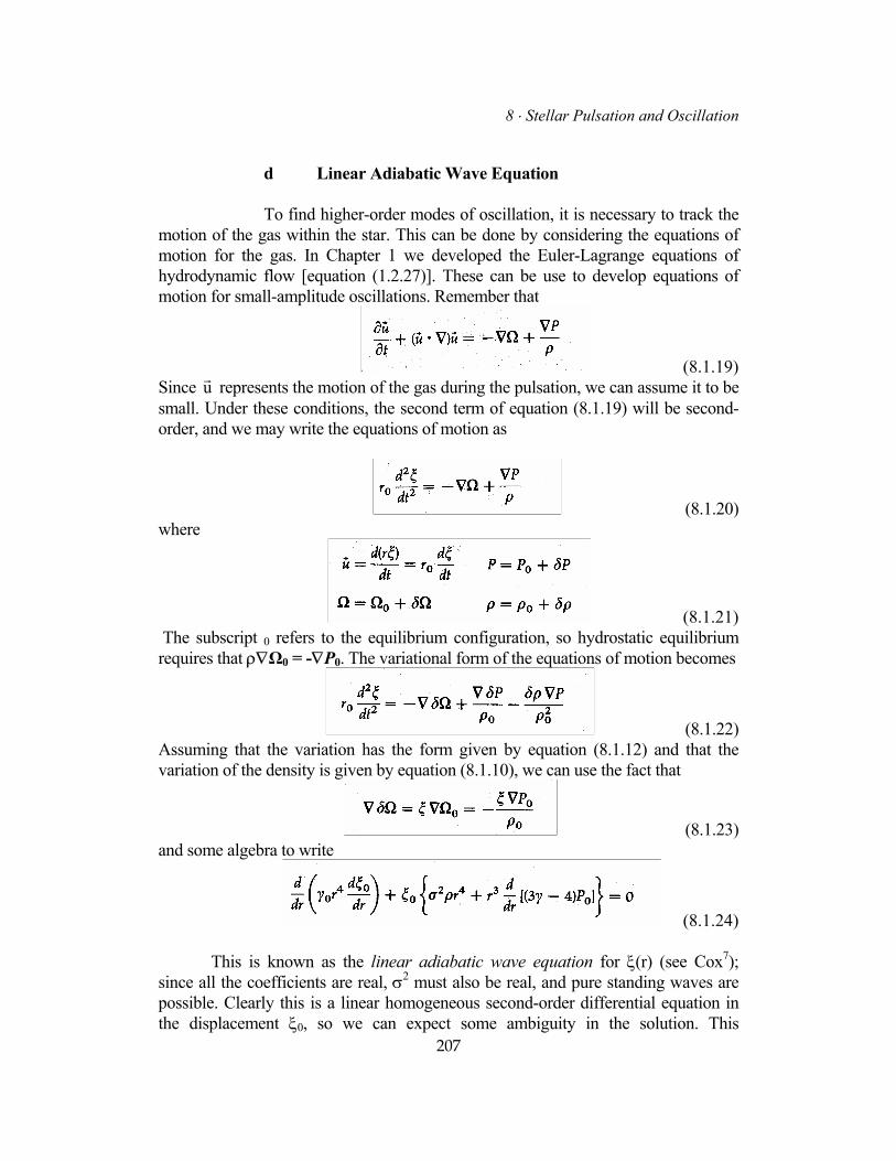
d Linear Adiabatic Wave Equation To find higher-order modes of oscillation, it is necessary to track the motion of the gas within the star. This can be done by considering the equations of motion for the gas. In Chapter 1 we developed the Euler-Lagrange equations of hydrodynamic flow [equation (1.2.27)]. These can be use to develop equations of motion for small-amplitude oscillations. Remember that

(8.1.19) Since represents the motion of the gas during the pulsation, we can assume it to be small. Under these conditions, the second term of equation (8.1.19) will be second-order, and we may write the equations of motion as

ur

(8.1.20) where

(8.1.21) The subscript 0 refers to the equilibrium configuration, so hydrostatic equilibrium requires that ρ∇Ω0 = -∇P0. The variational form of the equations of motion becomes

(8.1.22) Assuming that the variation has the form given by equation (8.1.12) and that the variation of the density is given by equation (8.1.10), we can use the fact that

(8.1.23) and some algebra to write

(8.1.24)

207

This is known as the linear adiabatic wave equation for ξ(r) (see Cox7); since all the coefficients are real, σ2 must also be real, and pure standing waves are possible. Clearly this is a linear homogeneous second-order differential equation in the displacement ξ0, so we can expect some ambiguity in the solution. This


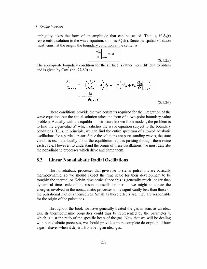
ambiguity takes the form of an amplitude that can be scaled. That is, if ξ0(r) represents a solution to the wave equation, so does Aξ0(r). Since the spatial variation must vanish at the origin, the boundary condition at the center is

(8.1.25) The appropriate boundary condition for the surface is rather more difficult to obtain and is given by Cox7 (pp. 77-80) as

(8.1.26) These conditions provide the two constants required for the integration of the wave equation, but the actual solution takes the form of a two-point boundary-value problem. Actually with the equilibrium structure known from models, the problem is to find the eigenvalue σ2 which satisfies the wave equation subject to the boundary conditions. Thus, in principle, we can find the entire spectrum of allowed adiabatic oscillations for a particular star. Since the solutions are pure standing waves, the state variables oscillate locally about the equilibrium values passing through them twice each cycle. However, to understand the origin of these oscillations, we must describe the nonadiabatic processes which drive and damp them. 8.2 Linear Nonadiabatic Radial Oscillations The nonadiabatic processes that give rise to stellar pulsations are basically thermodynamic, so we should expect the time scale for their development to be roughly the thermal or Kelvin time scale. Since this is generally much longer than dynamical time scale of the resonant oscillation period, we might anticipate the energies involved in the nonadiabatic processes to be significantly less than those of the pulsational motions themselves. Small as these effects are, they are responsible for the origin of the pulsations. Throughout the book we have generally treated the gas in stars as an ideal gas. Its thermodynamic properties could thus be represented by the parameter γ, which is just the ratio of the specific heats of the gas. Now that we will be dealing with nonadiabatic processes, we should provide a more complete description of how a gas behaves when it departs from being an ideal gas. 208


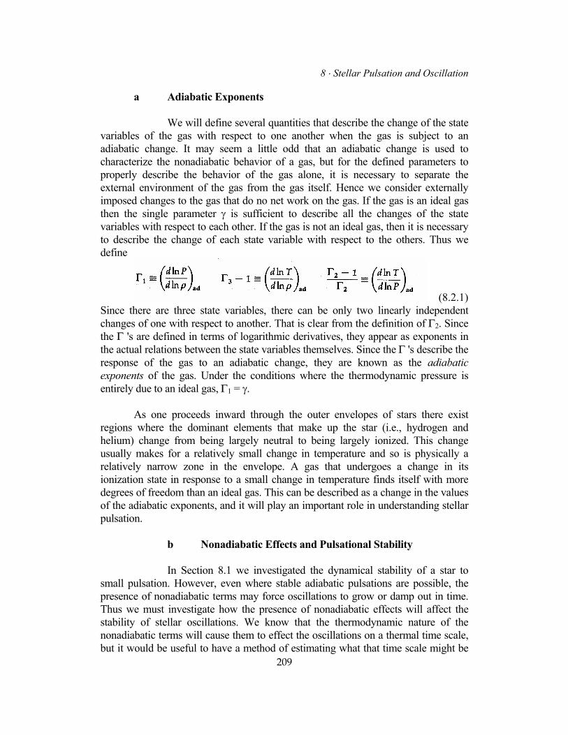
a Adiabatic Exponents We will define several quantities that describe the change of the state variables of the gas with respect to one another when the gas is subject to an adiabatic change. It may seem a little odd that an adiabatic change is used to characterize the nonadiabatic behavior of a gas, but for the defined parameters to properly describe the behavior of the gas alone, it is necessary to separate the external environment of the gas from the gas itself. Hence we consider externally imposed changes to the gas that do no net work on the gas. If the gas is an ideal gas then the single parameter γ is sufficient to describe all the changes of the state variables with respect to each other. If the gas is not an ideal gas, then it is necessary to describe the change of each state variable with respect to the others. Thus we define

(8.2.1) Since there are three state variables, there can be only two linearly independent changes of one with respect to another. That is clear from the definition of Γ2. Since the Γ 's are defined in terms of logarithmic derivatives, they appear as exponents in the actual relations between the state variables themselves. Since the Γ 's describe the response of the gas to an adiabatic change, they are known as the adiabatic exponents of the gas. Under the conditions where the thermodynamic pressure is entirely due to an ideal gas, Γ1 = γ. As one proceeds inward through the outer envelopes of stars there exist regions where the dominant elements that make up the star (i.e., hydrogen and helium) change from being largely neutral to being largely ionized. This change usually makes for a relatively small change in temperature and so is physically a relatively narrow zone in the envelope. A gas that undergoes a change in its ionization state in response to a small change in temperature finds itself with more degrees of freedom than an ideal gas. This can be described as a change in the values of the adiabatic exponents, and it will play an important role in understanding stellar pulsation. b Nonadiabatic Effects and Pulsational Stability

209

In Section 8.1 we investigated the dynamical stability of a star to small pulsation. However, even where stable adiabatic pulsations are possible, the presence of nonadiabatic terms may force oscillations to grow or damp out in time. Thus we must investigate how the presence of nonadiabatic effects will affect the stability of stellar oscillations. We know that the thermodynamic nature of the nonadiabatic terms will cause them to effect the oscillations on a thermal time scale, but it would be useful to have a method of estimating what that time scale might be


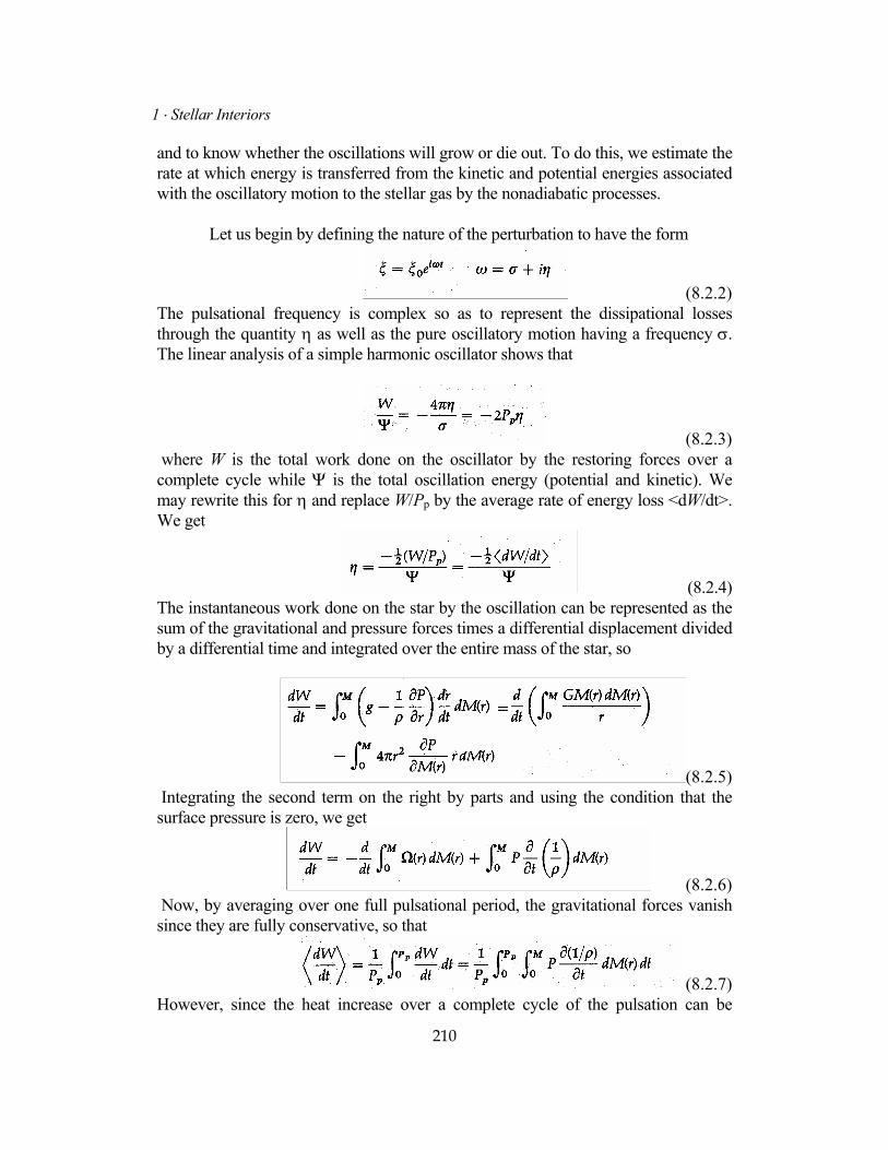
and to know whether the oscillations will grow or die out. To do this, we estimate the rate at which energy is transferred from the kinetic and potential energies associated with the oscillatory motion to the stellar gas by the nonadiabatic processes. Let us begin by defining the nature of the perturbation to have the form

(8.2.2) The pulsational frequency is complex so as to represent the dissipational losses through the quantity η as well as the pure oscillatory motion having a frequency σ. The linear analysis of a simple harmonic oscillator shows that

(8.2.3) where W is the total work done on the oscillator by the restoring forces over a complete cycle while Ψ is the total oscillation energy (potential and kinetic). We may rewrite this for η and replace W/Pp by the average rate of energy loss <dW/dt>. We get

(8.2.4) The instantaneous work done on the star by the oscillation can be represented as the sum of the gravitational and pressure forces times a differential displacement divided by a differential time and integrated over the entire mass of the star, so

(8.2.5) Integrating the second term on the right by parts and using the condition that the surface pressure is zero, we get

(8.2.6) Now, by averaging over one full pulsational period, the gravitational forces vanish since they are fully conservative, so that

(8.2.7) However, since the heat increase over a complete cycle of the pulsation can be

210


expressed in terms of the pressure and density changes,

(8.2.8) which means that the average energy transfer can be written as

(8.2.9) Since the pulsation represents a closed cycle the star, behaves as if it were a Carnot engine. If <dW/dt> > 0, then the pressure forces are doing positive work on the star and some source of that work must be found. Indeed, each mass shell may be treated separately by calculating the ∫PdV forces for that shell. So the star may be viewed as a sum of Carnot engines, some of which feed energy into the pulsation and others which remove it. If the sum of all the Carnot engines produce <dW/dt> > 0, the star is unstable and the oscillations will grow on a thermal time scale τth [see equation (3.2.12)] which we can estimate from the inverse of η. Thus

(8.2.10) Cox7 (see p. 117) finds that τth/Pp ranges from the order of 1 to about 1000 for common variables extending from the Mira variables to the RR Lyrae stars, respectively. This would imply that the pulsations in these stars ought to damp out in less than 1000 periods due to thermal losses. Since this is clearly not the case, we must find some sort of driving mechanism. c Constructing Pulsational Models While it is possible to develop a nonadiabatic wave equation (see Cox7, pp. 72, 73) similar to equation (8.1.24), we forgo doing so here. Instead let us consider a few aspects of the actual construction of a pulsating model. In principle, one has a complete equilibrium model which provides the run of state variables throughout the stars at equilibrium. It is against this background that one formulates the problem of how those state variables will vary with position and time. By assuming a variation of the form given in equation (8.2.2) for each of the state variables, one has the four dependent variables δr/r0, δρ/ρ0, ρT/T0, and δL/L0, with M(r) as the independent variable. The situation is similar to that encountered in Chapter 4 when we arranged the variables in the same manner to utilize the Henyey scheme for the construction of equilibrium models. Just as the construction of those models involved the solution of a two-point boundary-value problem for a particular eigenvalue, so this problem involves finding the complex eigenfrequency ω.

211


It is clear that unlike the linear adiabatic wave equation, the linear nonadiabatic wave equation will be complex. Hence the four dependent variables will be complex, with the real part describing the oscillatory motion and the imaginary part describing the damping of the solution. The central boundary conditions can make use of the fact that all variations must vanish at the center. Indeed, many early models8, 9 simply required the solution to go over to the adiabatic solution in the deep interior of the star. However, the surface boundary conditions are rather trickier. Perhaps the simplest condition that can be employed at the surface is the radiative condition

(8.2.11) In addition to the difficulties of posing the correct boundary conditions, significant numerical problems are encountered in the actual solution. These problems were overcome by Castor10 and Iben11 so that reliable pulsational models can now be obtained. d Pulsational Behavior of Stars We have already indicated that the helium and hydrogen ionization zones might be expected to play a significant role in determining the actual nature of pulsating stars, since they represent zones where the value of Γ3 varies with position. However, such zones exist in all stars, but not all stars exhibit radial oscillations. Indeed, further thought about the role of ionization zones would lead one to believe that the destabilizing effect on a radial oscillation entering the ionization zone from below brought about by the rapidly declining value of Γ3 would be offset by the damping effect of a rising Γ3 at the top of the zone. For the majority of stars this appears to be the case. Something else must be operative, and to understand its nature, we must consider the nature of nonadiabatic forces near the surface of the star. Consider the part of the stellar envelope that is relatively near the surface. This region is what Cox7 (pp. 140, 141) has called the transition zone. As one moves up through the stellar envelope toward the surface, the thermal cooling time steadily decreases. The nearer one is to the surface, the less time is required for energy to diffuse to the surface and escape. Thus the nonadiabatic effects will be more pronounced since pulsational energy that appears as thermal energy will be quickly radiated away. Changes in the luminosity generated deeper in the star will become "frozen in" the star and not travel with the wave. When this transition zone coincides with an ionization zone, the potential exists for the nonadiabatic effects of ionization to also be "frozen in". Thus, if the ionization zone lies at the right depth, the driving

212


effects caused by the decline in Γ3 upon entering the zone will not be reversed upon leaving, because the luminosity changes so induced become "frozen in". Since the conditions for ionization are set by atomic physics, we should expect that stars with the appropriate effective temperatures and gravities to produce an ionization zone at the correct diffusion depth corresponding to the transition zone will exhibit radial pulsations. There is indeed a region on the H-R diagram known as the instability strip which encompasses the Cepheid variables, W Virginis stars, δ Scuti stars, RR-Lyrae stars, and Dwarf Cepheids where this condition appears to be met for the He II ionization zone. The He II ionization zone seems to be the dominant zone for most of the common variable stars. The H and He I ionization zones lie so close together that they may be virtually considered as one. They invariably lie above the He II ionization zone in a region where the luminosity changes have already been frozen in and so play little role in the hot stars. However, this zone is suspected of introducing a phase shift between the luminosity variations and the radial velocity variation from that which is expected. Normally one would expect the time of maximum compression to be the time of maximum luminosity. However, the luminosity maximum lags somewhat, and this may result from its being delayed in the hydrogen ionization zone. In late-type variables where the He II zone is so deep as to be below the transition zone, the hydrogen ionization zone may be the primary driver of the pulsations. However, for these stars the situation becomes complicated by the large geometric extent of the atmosphere and the complex nature of the opacity. We have seen how the onset of He II ionization at the appropriate place in the star can cause conditions to exist that will drive pulsations simply by a rapid decline of Γ3. This cause of pulsation is called the γ-mechanism. However, there is another contributor to the destabilizing effect of ionization. In most of the stellar interior, an increase in temperature is accompanied by a decline in opacity. Certainly Kramer’s law [equation (4.1.19)] implies this. Thus any temperature increase accompanying the compression of a passing pulsational perturbation would cause a decline in the local opacity and a release of the radiation trapped there. This would tend to stabilize the region against pulsations by removing the pulsational energy in the form of radiation. However, at low temperatures a rise in temperature results in an increase in opacity. This effect was largely responsible for the nearly vertical tracks of collapsing convective protostars (see Section 5.2c). If the opacity increases with increasing temperature, the opacity will tend to trap the energy at that point and prevent the energy from diffusing away. This is a destabilizing effect that tends to feed the pulsations, and it has been called the κ mechanism. Of these two, the γ mechanism seems to be the more important for the pulsation of Cepheid variables. When the oscillations become large, the linear theory we have been

213


describing becomes invalid. However, the complications introduced by these nonlinearities are well beyond the scope of this book, and we leave them to others to discuss.

8.3 Nonradial Oscillations So far we have considered only those oscillations that involve the radial coordinate only. While these oscillations seem sufficient to explain the majority of known pulsating stars, other less dramatic phenomena result from more complicated oscillations. Indeed, one would expect that most pulsational energy would appear in the fundamental radial mode of oscillation, and it is precisely those modes involving the modulation of the greatest amount of energy that can be most easily detected. However, the detection of short-period oscillations of low amplitude in the sun suggests that more complicated types of oscillations can occur. Their importance to the structural models of the sun and their probable detection in some early-type stars require that we spend a little time discussing them. However, the subject is too broad and many of the results are too uncertain to do more than sketch the nature of the problem. To give the greatest insight into the nature of the problem, I will concentrate on the adiabatic oscillations. The true cause of the oscillations lies in nonadiabatic theory, as it did for radial oscillations, and the results are still rather uncertain. In addition, the theory for oscillations among stars that are not spherically symmetric is still in its infancy. It was clear from Chapter 6 that the loss of spherical symmetry resulted in a substantial increase in the complexity of the theoretical description. No less is to be expected from pulsation theory. From the small amount of energy involved in the present cases of nonradial oscillations, it will be appropriate to use perturbation theory and to assume that the amplitudes of the oscillations are small. a Nature and Form of Oscillations Just as there exists a wave equation for radial oscillations, so there is a wave equation for nonradial oscillations. However, instead of being a scalar equation in the radial coordinate r alone, it will be a vector equation whose solution will represent the behavior of the displacement vector rrδ and the associated variations of the state variables in the various dimensions that define the star. Since our problem will be an adiabatic one, the solutions will be undamped waves propagating not only along the radial coordinate but also over the surface coordinates. In Chapter 7 we saw that it was possible to represent the polar angle variation in terms of a series of Legendre polynomials. This was a special case of a much more general representation of the angular variation of solutions to a wide range of important physical equations. Laplace's equation, the Schrödinger equation, 214


and the wave equation of classical electrodynamics are only a few of the equations whose solutions can be described in terms of spherical harmonics. Spherical harmonics are basically the product of the elements of two sets of functions. One set of functions describes the solution variation in the polar angle and is represented by the orthonormal Legendre polynomials. The orthogonal functions that describe the behavior in the azimuthal coordinate are just . Thus the spherical harmonics are defined

φmie13 as

(8.3.1) As long as the star remains spherical, the equation describing the nonradial oscillations will also be separable in spherical coordinates, and the orthogonality of the spherical harmonics will guarantee that the full solution can be represented in terms of them. Since some of the solutions to the radial wave equation were standing waves, we should not be surprised if that were also the case for the nonradial oscillations. The linearity of the small-oscillation equations guarantees that the sum of any two solutions is also a solution. So a standing wave is just the interference pattern of two oppositely directed traveling waves of similar amplitude. Just as there could be higher-order modes of the radial wave equation excited, so higher-order waves in the azimuthal and polar angles can be present. However, different modes in each of the coordinates may combine to provide a much richer multiplicity of possible oscillations for the nonradial case. Thus the solution will have the form

(8.3.2) The quantity ℜ is a function of the radial coordinate only and represents the eigenfunctions that are possible in the radial direction. Different orders are usually denoted by the letter n. The periodic behavior of the spherical harmonics implies that the parameters l and m will denote the different eigenfunctions in the polar and azimuthal coordinates, respectively. Deubner and Gough13 give a nice way of seeing this. Consider cases when the wavelength of the oscillation is much less than the stellar dimensions. Under these conditions Lamb14 showed that the equations of motion can be reduced to the familiar form

(8.3.3) where

215


(8.3.4) and cs is just the local speed of sound. This is simply the equation for a simple harmonic oscillator; here K is the local wave number and in this instance is related to the frequency of oscillation ω, scale height h, and local gravity g by

(8.3.5) where

(8.3.5a) Thus we may expect that the general solution for the equations of motion will consist of a complicated interplay of waves propagating in all three coordinates. Also the specific nature of these waves will depend on the structure of the star, with the low-frequency wave anchored deep in the interior and the high-frequency waves determined largely by the local structure of the star nearer the surface. To try to bring some order to the multiplicity of oscillations that may be present in stars, let us consider an idealized case. b Homogeneous Model and Classification of Modes Consider a homogeneous star of uniform density. Admittedly this is an unrealistic case in the real world, but it has the virtue that the eigenfrequencies of the equations of motion can be found and have a particularly simple form. Cowling15 found that the eigenfrequencies could be organized into several groups based on the physical mechanisms primarily responsible for their propagation. These modes all have their counterparts in the solutions of more realistic models, and so Cowling's classification scheme provides a useful basis for identifying the types of modes to be expected in real stars. Following Cox7 (p. 235), we can define a dimensionless frequency

(8.3.6) The radial oscillation modes are then given by

(8.3.7) 216


which for large n are approximately given by

(8.3.8) The negative root in equation (8.3.7) and its asymptotic counterpart in the g modes of equations (8.3.8) imply that ƒ2

ln < 0. So the star is dynamically unstable, and this is a result of the homogeneous model's being unstable to convection. In real stars this is not generally the case, and the g modes can be real. The terminology has its roots in the nature of the oscillations corresponding to each of the modes. The p modes are known as pressure modes; they can be viewed as pressure or acoustic waves and are characterized by relatively large radial pressure disturbances. For n = 0 they correspond to the radial oscillations studied in the previous two sections. Thus, as n increases, the p modes can be roughly viewed as radial standing waves having n nodes. It would be reasonable to call them longitudinal waves. On the other hand, stable oscillations characterized by the g modes can be viewed as transverse waves. They are also known as gravity waves (not to be confused with gravitational waves, which are a phenomenon of the general theory of relativity); because the primary force acting as a restoring force for the oscillation is the local gravity. These waves are characterized by relatively small pressure and density variations and are largely transverse in their physical displacement. The most common analogy to these waves is water waves where the restoring force is clearly that of gravity and virtually no pressure or density changes are involved. Curiously the case for n = l and n >> 1 leads to

(8.3.9) and a characteristic frequency that is independent of the order n. Physically such a condition would correspond to small blobs of material having a typical size much less than the stellar dimension, moving radially, and exhibiting small pressure and density changes. This is a fairly good description of a convective element and is often taken as a basis for describing the expected spectrum for convective blobs in a region unstable to convection. Thus the presence of g modes in a region stable against convection may be the result of excitation by a lower-lying convective region. The actual frequencies of oscillation for the g modes are always less than those for the corresponding p mode (see Figure 8.1). Lying between these two classes of modes is a solitary mode called the f mode. This mode is generally attributed to Lord Kelvin and is characterized by ∇ ⋅ δr = 0 for the homogeneous model. This implies that both δP and δρ are zero as for an incompressible fluid. However, this is not true for stellar models in general, and 217


so this mode is sometimes referred to as the pseudo-Kelvin mode. Its dimensionless eigenfrequency for the homogeneous model is given by

(8.3.10) This eigenfrequency is independent of Γ1 which is to be expected since δP and δp are both zero. That condition also implies a link between the radial and angular displacements so that oscillations in the radial coordinate are uniquely linked to displacements in the radial coordinate. There are no stable modes for l < 2.

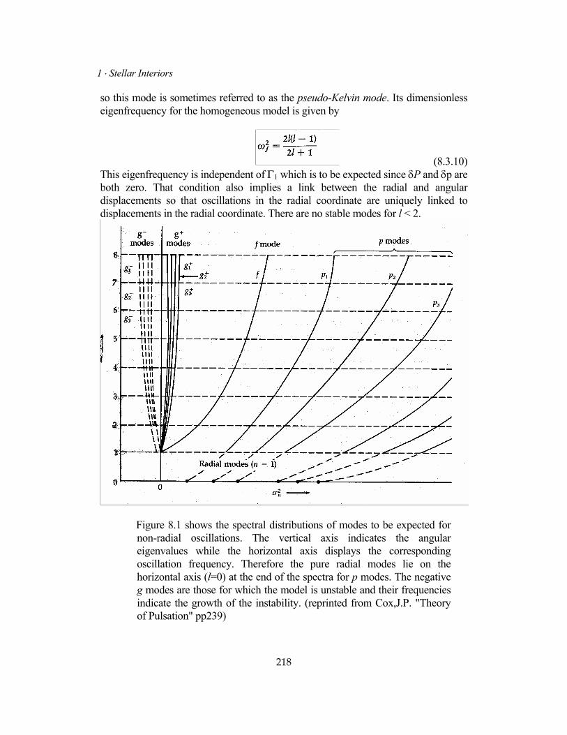
Figure 8.1 shows the spectral distributions of modes to be expected for non-radial oscillations. The vertical axis indicates the angular eigenvalues while the horizontal axis displays the corresponding oscillation frequency. Therefore the pure radial modes lie on the horizontal axis (l=0) at the end of the spectra for p modes. The negative g modes are those for which the model is unstable and their frequencies indicate the growth of the instability. (reprinted from Cox,J.P. "Theory of Pulsation" pp239)

218


c Toroidal Oscillations There remains one last class of oscillations that we have not considered. So far we have been faithful to our assumption of spherical symmetry and discussed no modes that have a dependence on the azimuthal angle φ so that m = 0. To have included cases where m ≠ 0 would have been to admit the existence of a preferred plane and thereby violate the assumption of spherical symmetry. Thus the modes described so far will present surface phenomena that are independent of the orientation of the star. This will not be the case for m ≠ 0. However, there is no a priori reason why azimuthal modes cannot exist. Indeed, for each value of l there are 2l + 1 allowed values of m (that is, m = 0, ∀1, ∀2, ∀ ⋅ ⋅ ⋅ ∀l) which represent waves that propagate in the ∀ φ direction. Of course for a nonrotating star there is no preferred direction of propagation, so these modes are degenerate and there are only l + 1 distinct possibilities. Papaloizou and Pringle16 have shown that for rotation, this degeneracy is broken and the resulting modes correspond to traveling waves around the rotational axis of the star similar to Rossby waves in the earth's atmosphere, so they designated them r modes. These waves travel with a characteristic velocity that is approximately 1/m times the rotational period of the star. Thus such a wave would be seen by an observer to be moving at a rate that is slightly faster (+m) and slightly slower (-m) than the rotational speed of the star. Any comprehensive analysis of the effects of rotation must deal with the effects of angular momentum conservation as well as shape distortion and is therefore quite difficult. However, there can be little doubt that rotation will influence the values for the eigenfrequencies for the p and g modes. Although the overall effects of rotation are extremely complicated, there is some evidence from nonadiabatic studies that the prograde modes are somewhat less stable and therefore more likely to be excited, than the retrograde modes. It is possible to have such modes in a star for which the total angular momentum is zero. In the case where l = 1 such modes represent uniform rotation of the object. For l > 1 the modes would represent torsional oscillations. In the simplest case where l = 2, one hemisphere would rotate, say clockwise, while the other hemisphere rotated counterclockwise. Unfortunately, to stabilize such an oscillation, some sort of shear would have to be sustained by the stellar material. Such restoring shears are simply absent in normal stars. However, in white dwarfs and neutron stars, at least part of the star is expected to be in a crystalline phase and this matter could perhaps sustain such oscillations.

219


d Nonradial Oscillations and Stellar Structure From all that we have discussed so far, clearly the spectrum of oscillations present in a star depends critically on the structure of the star. If it were possible to observe the full spectrum of these oscillations, including their frequency and amplitude, quite sensitive tests of the internal structure of the equilibrium model would be possible. The analogy has been made to geophysicists who deduce the internal structure of the earth from the propagation of seismic waves produced by earthquakes. So strong is this analogy that the term helioseismology has come into fairly common use to describe oscillation analysis as applied to the sun. Clearly, in the case of the sun, we have an opportunity to map the oscillation structure with a high degree of accuracy. While research in this area is ongoing, both p and g modes have been detected. The p modes are usually characterized by the generic term 5-minute oscillations. Oscillations described by 1 < l < 1000 have been detected, and the power (amplitude) of those oscillations has been determined. This is done by mapping the radial velocity field of the entire solar disk over extended periods and performing a Fourier analysis of the result for periodic structures. Clearly the velocity of an oscillatory displacement is simply related to the displacement and to the frequency itself. Thus the highly accurately determined velocity measurements provide accurate knowledge of the amplitude and frequencies of the oscillations that are present. The ability to resolve closely spaced frequencies simply requires a long, continuous series of observations. In addition to the p modes, g modes with characteristic periods ranging from just under 3 hours to nearly 6 days have been reported. There is some disagreement among observers as to what constitutes actual periodic waves and which modes are "aliases" of other periodic phenomena and the data-sampling procedure. However, the existence of the g modes is quite likely. In general, the low-order modes represent wave structures that penetrate deeply into the interior, while the higher-frequency modes are confined to the outer layers of the sun. Indeed, the highest-frequency p modes are probably confined to the solar atmosphere itself. Thus the full spectrum of the solar oscillations allows a continuous depth probe of the internal solar structure. The standard solar model reproduces the overall properties of the oscillation spectrum, but fails to fit that spectrum in detail. There is some indication that the standard solar model may have a helium abundance that is somewhat low. Ulrich and Rhodes17 conclude that the failure of the standard solar model to fit the observations of the oscillation spectrum is real and lies outside the errors of either theory or observation. This would place it in the same category as the solar neutrino problem. Hopefully the solution of one can provide a solution for the other.

220


There are strong indications that nonradial modes have been detected in other stars. β Cephei stars are suspected to exhibit the effects of traveling waves on their surfaces in their spectra. Papaloizou and Pringle16 explain the short period oscillations seen in some cataclysmic variables to the r modes of surface traveling waves. In addition18, 19 sharp absorption features that move through the broad absorption lines of some rapidly rotating stars have been interpreted as representing nonradial oscillations. If this is proves to be the case, then the observations indicate the existence of a phenomenon for which there is no clear theoretical description. For reasons already mentioned, pulsation theory in the presence of extreme rotation is extremely difficult and far from well developed. However, should nonradial oscillations be unambiguously measured for these stars, the potential for detailed understanding of their internal structure is considerable. Given the uncertainties regarding the effects of rotation on the internal structure of these stars, every effort should be made to explore these observations as a probe of the stellar interior. Problems 1. Show how equations (8.3.8) and (8.3.9) can be obtained from equation

(8.3.7). 2. Use the Virial theorem to find the fundamental radial pulsation period for a homogeneous star where the equation of state is

3. Compute the lowest-order mode for polytropes with indices n of 1.5, 2.5, and

3 for stellar masses M = 1.5M⊙ and 30M⊙ . 4. Assuming that the shear forces resulting from the crystalline structure of a

white dwarf near the Chandrasekhar limit were sufficient to permit torsional oscillations, estimate the frequency of the lowest-order mode.

5. Show how the wave equation [equation (8.1.24)] is obtained from the

equations of motion [equation (8.1.19)]. References and Supplemental Reading 1. Eddington, A.S.: On the Pulsations of a Gaseous Star and the Problem of the

Cepheid Variables. Part I, Mon. Not. R. astr. Soc., 79, 1918, pp. 2 - 22.

221


2. Eddington, A.S.: The Internal Constitution of the Stars, Dover, New York, 1959, chap. 8.

3. Ledoux, P.: On the Radial Pulsation of Stars", Ap.J. 102, 1945, pp.143 - 153 4. Ledoux, P., and Walraven, Th.: "Variable Stars", Handb. d. Phys., Vol. 51, Springer-Verlag Berlin, 1958, pp.353 - 601. 5. Chandrasekhar, S.: Hydrodynamic and Hydromagnetic Stability, Oxford University Press, London, 1961. 6. Collins, G.W.,II: The Virial Theorem in Stellar Astrophysics, Pachart Press, Tucson, Ariz., 1978. 7. Cox, J.P.: Theory of Stellar Pulsation, Princeton University Press, Princeton N.J., 1980. 8. Baker,N., and Kippenhahn, R.: The Pulsations of Models of δ Cephei Stars", z. f. Astrophys. 54, 1962, pp.114 - 151. 9. Cox, J.P.: On Second Helium Ionization as a Cause of Pulsational Instability

in Stars, Ap.J. 138, 1963, pp.487 - 536. 10. Castor, J.I.: On the Calculation of Linear, Nonadiabatic Pulsations of Stellar

Models, Ap.J. 166, 1971, pp.109 - 129. 11. Iben, I., Jr.: On the Specification of the Blue Edge Of The RR Lyrae

Instability Strip, Ap.J. 166, 1971, pp.131 - 151. 12. Arfken, G.: Mathematical Methods for Physicists, 2nd. ed. Academic, New

York, 1970, pp.569 - 572. 13. Deubner, F.-L., and Gough, D. "Helioseismology: Oscillations as a

Diagnostic of the Solar Interior", Annual Reviews of Astronomy and Astrophysics, vol. 22, Annual Reviews, Palo Alto, Calif., 1984, pp.593 - 619.

14. Lamb, H.: Hydrodynamics 5th.ed., Cambridge University Press, New York,

1924, pp.467 - 484. 15. Cowling, T.G.: The Non-radial Oscillations of Polytropic Stars, Mon. Not.

R. astr. Soc., 101, 1941, pp.367 - 373. 222


16. Papaloizou,J.C.B., and Pringle,J.E.: Non-radial Oscillations of Rotating

Star and Their Relevance to the Short-Period Oscillations of Cataclysmic Variables, Mon. Not. R. astr. Soc., 182, 1978, pp.423 - 442. 17. Ulrich, R.K., and Rhodes, E.J., Jr.: Testing Solar Models with Global Solar

Oscillations in the 5-Minute Band, Ap.J. 265, 1983, pp.551 - 563. 18. Penrod, G.D. "Nonradial Pulsations and the Be Phenomenon", Physics of Be

Stars, Ed: A.Slettebak and T.P.Snow, Cambridge University Press, Cambridge, 1987, p. 463.

19. Smith, M.A., Gies, D.R. and Penrod, G.D.: "Spectral Transients in the Line

Profiles of l Eridani", Physics of Be Stars, Ed: A.Slettebak and T.P.Snow, Cambridge University Press, Cambridge, 1987, pp. 464-467.

For a background of the observational material that initiated much of the interest in pulsating stars, read Shapley, H.: On the Nature and Cause of Cepheid Variables Ap. J. 40, 1940, pp.448

- 465. One of the most readable books on stellar pulsation remains Rosseland, S.: The Pulsation Theory of Variable Stars, Dover, New York, 1964. An excellent review of the nonadiabatic effects in stellar pulsation theory can be found in

Christy, R.F.: Pulsation Theory, Annual Reviews of Astronomy and Astrophysics, Vol. 4, Annual Reviews, Palo Alto, Calif., 1966,

pp.353 - 392.

223

224


Epilogue to Part I: Stellar Interiors We have presented the study of stellar interiors as a subject that builds from a minimal base of assumptions to the description of some of the most exotic objects in the universe. To describe the structure of most stars in a qualitative manner, we need only construct equilibrium models which follow a polytropic law. To improve that description and to understand the evolution of stars, it is necessary to add a substantial amount of physics and to construct steady-state models. We illustrated the nature of the physics to be added, but many more details need to be included to create models of contemporary accuracy. We did not examine in detail those instances for which steady-state models fail because of rapid evolution which requires hydrodynamic equilibrium to be invoked. However, we did sketch some consequences of this rapid evolution. We saw that it is possible to understand all the stellar evolution that takes place on a time scale longer than the dynamical time in light of a sequence of equilibrium models linked by estimates of the dominant mode of energy transport required for the construction of steady-state models. This approach yields a good qualitative picture of stellar evolution from pre-main sequence contraction through the helium-burning phases. Finally, we investigated some problems that lie outside the normal theory of stellar structure and evolution primarily to indicate the direction in which research in these areas has been proceeding. The one axiom that has dominated Part I of the book is STE. This enabled us to characterize the stellar gas and radiation field entirely in terms of the state variables P, T, and ρ. This was possible because the mean free path for particles and photons was much smaller than the characteristic size of the star. As the boundary is approached, systematic differences from the statistical energy distribution expected from STE will appear, but by the time this begins to happen, the structure of the star will usually be determined. However, to know what the star will look like, we have to consider this region in greater detail. Such an investigation is the aim of Part II.

Documents

8 - Stellar Pulsation and Oscillationads.harvard.edu/books/1989fsa..book/AbookC08.pdf · 2003-01-29 · 8 ⋅ Stellar Pulsation and Oscillation (8.1.12) Substitution of this form