15 Breakdown of Local Thermodynamic Equilibriumads.harvard.edu/books/1989fsa..book/AbookC15.pdf · II ⋅ Stellar Atmospheres 15.1 Phenomena Which Produce Departures from Local Thermodynamic

II ⋅ Stellar Atmospheres

Copyright (2003) George W. Collins, II

15

Breakdown of Local Thermodynamic Equilibrium

. . . Thus far we have made considerable use of the concepts of equilibrium. In the stellar interior, the departures from a steady equilibrium distribution for the photons and gas particles were so small that it was safe to assume that all the constituents of the gas behaved as if they were in STE. However, near the surface of the star, photons escape in such a manner that their energy distribution departs from that expected for thermodynamic equilibrium, producing all the complexities that are seen in stellar spectra. However, the mean free path for collisions between the particles that make up the gas remained short compared to that of the photons, and so the collisions could be regarded as random. More importantly, the majority of the collisions between photons and the gas particles could be viewed as occurring between particles in thermodynamic equilibrium. Therefore, while the radiation field departs from that of a black body, the interactions determining the state of the gas continue to lead to the establishment of an energy distribution for the gas particles characteristic of thermodynamic equilibrium. This happy state allowed the complex properties of the gas to be determined by the local temperature alone and is known as LTE.

398

15 ⋅ Breakdown of Local Thermodynamic Equilibrium However, in the upper reaches of the atmosphere, the density declines to such a point that collisions between gas particles and the remaining "equilibrium" photons will be insufficient for the establishment of LTE. When this occurs, the energy level populations of the excited atoms are no longer governed by the Saha-Boltzmann ionization-excitation formula, but are specified by the specific properties of the atoms and their interactions. Although the state of the gas is still given by a time-independent distribution function and can be said to be in steady or statistical equilibrium, that equilibrium distribution is no longer the maximal one determined by random collisions. We have seen that the duration of an atom in any given state of excitation is determined by the properties of that atomic state. Thus, any collection of similar atoms will attempt to rearrange their states of excitation in accordance with the atomic properties of their species. Only when the interactions with randomly moving particles are sufficient to overwhelm this tendency will the conditions of LTE prevail. When these interactions fail to dominate, a new equilibrium condition will be established that is different from LTE. Unfortunately, to find this distribution, we have to calculate the rates at which excitation and de-excitation occur for each atomic level in each species and to determine the population levels that are stationary in time. We must include collisions that take place with other constituents of the gas as well as with the radiation field while including the propensity of atoms to spontaneously change their state of excitation. To do this completely and correctly for all atoms is a task of monumental proportions and currently is beyond the capability of even the fastest computers. Thus we will have to make some approximations. In order for the approximations to be appropriate, we first consider the state of the gas that prevails when LTE first begins to fail. A vast volume of literature exists relating to the failure of LTE and it would be impossible to cover it all. Although the absorption of some photon produced by bound-bound transitions occurs in that part of the spectrum through which the majority of the stellar flux flows, only occasionally is the absorption by specific lines large enough to actually influence the structure of the atmosphere itself. However, in these instances, departures from LTE can affect changes in the atmosphere's structure as well as in the line itself. In the case of hydrogen, departures in the population of the excited levels will also change the "continuous" opacity coefficient and produce further changes in the upper atmosphere structure. To a lesser extent, this may also be true of helium. Therefore, any careful modeling of a stellar atmosphere must include these effects at a very basic level. However, the understanding of the physics of non-LTE is most easily obtained through its effects on specific atomic transitions. In addition, since departures from LTE primarily occur in the upper layers of the atmosphere and therefore affect the formation of the stellar spectra, we concentrate on this aspect of the subject. 399


15.1 Phenomena Which Produce Departures from Local Thermodynamic Equilibrium

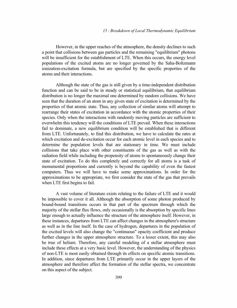
a Principle of Detailed Balancing Under the assumption of LTE, the material particles of the gas are assumed to be in a state that can be characterized by a single parameter known as the temperature. Under these conditions, the populations of the various energy levels of the atoms of the gas will be given by Maxwell-Boltzmann statistics regardless of the atomic parameters that dictate the likelihood that an electron will make a specific transition. Clearly the level populations are constant in time. Thus the flow into any energy level must be balanced by the flow out of that level. This condition must hold in any time-independent state. However, in thermodynamic equilibrium, not only must the net flow be zero, so must the net flows that arise from individual levels. That is, every absorption must be balanced by an emission. Every process must be matched by its inverse. This concept is known as the principle of detailed balancing. Consider what would transpire if this were not so. Assume that the values of the atomic parameters governing a specific set of transitions are such that absorptions from level 1 to level 3 of a hypothetical atom having only three levels are vastly more likely than absorptions to level 2 (see figure 15.1). Then a time-independent equilibrium could only be established by transitions from level 1 to level 3 followed by transitions from level 3 to level 2 and then to level 1. There would basically be a cyclical flow of electrons from levels 1 → 3 → 2 → 1. The energy to supply the absorptions would come from either the radiation field or collisions with other particles. To understand the relation of this example to LTE, consider a radiation-less gas where all excitations and de-excitations result from collisions. Then such a cyclical flow would result in energy corresponding to the 1 → 3 transition being systematically transferred to the energy ranges corresponding to the transitions 3 → 2 and 2 → 1. This would lead to a departure of the energy momentum distribution from that required by Maxwell-Boltzmann statistics and hence a departure from LTE. But since we have assumed LTE, this process cannot happen and the upward transitions must balance the downward transitions. Any process that tends to drive the populations away from the values they would have under the principle of detailed balancing will generate a departure from LTE. In the example, we considered the case of a radiationless gas so that the departures had to arise in the velocity distributions of the colliding particles. In the upper reaches of the atmosphere, a larger and larger fraction of the atomic collisions are occurring with photons that are departing further and further from the Planck function representing their thermodynamic equilibrium distribution. These interactions will force the level populations to depart from the values they would have under LTE. 400

15 ⋅ Breakdown of Local Thermodynamic Equilibrium

Figure 15.1 shows the conditions that must prevail in the case of detailed balancing (panel a) and for interlocking (panel b).The transition from level(1) to level (3) might be a resonance line and hence quite strong. The conditions that prevail in the atmosphere can then affect the line strengths of the other lines that otherwise might be accurately described by LTE.

b Interlocking Consider a set of lines that have the same upper level (see Figure 15.1). Any set of lines that arise from the same upper level is said to be interlocked (see R.Woolley and D.Stibbs1). Lines that are interlocked are subject to the cyclical processes such as we used in the discussion of detailed balancing and are therefore candidates to generate departures from LTE. Consider a set of lines formed from transitions such as those shown in Figure 15.1. If we assume that the transition from 163 is a resonance line, then it is likely to be formed quite high up in the atmosphere where the departures from LTE are the largest. However, since this line is interlocked with the lines resulting from transitions 3 → 2 and 3 →1, we can expect the departures affecting the resonance line to be reflected in the line strengths of the other lines. In general, the effect of a strong line formed high in the atmosphere under conditions of non-LTE that is interlocked with weaker lines formed deeper in the atmosphere is to fill in those lines, so that they appear even weaker than would otherwise be expected. A specific example involves the red lines of Ca II(λλ8498, λλ8662, λλ8542), which are interlocked with the strong Fraunhofer H and K resonance lines. The red lines tend to appear abnormally weak because of the photons fed into them in the upper atmosphere from the interlocked Fraunhofer H & K lines.

401


c Collisional versus Photoionization We have suggested that it is the relative dominance of the interaction of photons over particles that leads to departures from LTE that are manifest in the lines. Consider how this notion can be quantified. The number of photoionizations from a particular state of excitation that takes place in a given volume per second will depend on the number of available atoms and the number of ionizing photons. We can express this condition as

(15.1.1) The frequency ν0 corresponds to the energy required to ionize the atomic state under consideration. The integral on the far right-hand side is essentially the number of ionizing photons (modulo 4π), so that this expression really serves as a definition of Rik as the rate coefficient for photoionizations from the ith state to the continuum. In a similar manner, we may describe the number of collisional ionizations by

(15.1.2) Here, Cik is the rate at which atoms in the ith state are ionized by collisions with particles in the gas. The quantity σ(v) is the collision cross section of the particular atomic state, and it must be determined either empirically or by means of a lengthy quantum mechanical calculation; and f(v) is the velocity distribution function of the particles. In the upper reaches of the atmosphere, the energy distribution functions of the constituents of the gas depart from their thermodynamic equilibrium values. The electrons are among the last particles to undergo this departure because their mean free path is always less than that for photons and because the electrons suffer many more collisions per unit time than the ions. Under conditions of thermodynamic equilibrium, the speeds of the electrons will be higher than those of the ions by (mh A/me)½ as a result of the equipartition of energy. Thus we may generally ignore collisions of ions of atomic weight A with anything other than electrons. Since the electrons are among the last particles to depart from thermodynamic equilibrium, we can assume that the velocity distribution f(v) is given by Maxwell-Boltzmann statistics. Under this assumption Ωik will depend on atomic properties and the temperature alone. If we replace Jν with Bν(T), then we can estimate the ratio of photoionizations to collisional ionizations Rik/Cik under conditions that prevail in the atmospheres of normal stars. Karl Heintz Böhm2 has used this procedure along with the semi-classical Thomson cross section for the ion to estimate this ratio. Böhm finds that only for the upper-lying energy levels and at high temperatures and densities will collisional ionizations dominate over photoionizations. Thus, for most

402

15 ⋅ Breakdown of Local Thermodynamic Equilibrium lines in most stars we cannot expect electronic collisions to maintain the atomic-level populations that would be expected from LTE. So we are left with little choice but to develop expressions for the energy-level populations based on the notion that the sum of all transitions into and out of a level must be zero. This is the weakest condition that will yield an atmosphere that is time-independent. 15.2 Rate Equations for Statistical Equilibrium The condition that the sum of all transitions into and out of any specific level must be zero implies that there is no net change of any level populations. This means that we can write an expression that describes the flow into and out of each level, incorporating the detailed physics that governs the flow from one level to another. These expressions are known as the rate equations for statistical equilibrium. The unknowns are the level populations for each energy level which will appear in every expression for which a transition between the respective states is allowed. Thus we have a system of n simultaneous equations for the level populations of n states. Unfortunately, as we saw in estimating the rates of collisional ionization and photoionization, it is necessary to know the radiation field to determine the coefficients in the rate equations. Thus any solution will require self-consistency between the radiative transfer solution and the statistical equilibrium solution. Fortunately, a method for the solution of the radiative transfer and statistical equilibrium equations can be integrated easily in the iterative algorithm used to model the atmosphere (see Chapter 12). All that is required is to determine the source function in the line appropriate for the non-LTE state. Since an atom has an infinite number of allowed states as well as an infinite number of continuum states that must be considered, some practical limit will have to be found. For the purpose of showing how the rate equations can be developed, we consider two simple cases. a Two-Level Atom It is possible to describe the transitions between two bound states we did for photo- and collisional ionization. Indeed, for the radiative processes, basically we have already done so in (Section 11.3) through the use of the Einstein coefficients. However, since we are dealing with only two levels, we must be careful to describe exactly what happens to a photon that is absorbed by the transition from level 1 to level 2. Since the level is not arbitrarily sharp, there may be some redistribution of energy within the level. Now since the effects of non-LTE will affect the level populations at various depths within the atmosphere, we expect these effects will affect the line profile as well as the line strength. Thus, we must be clear as to what other effects might change the line profile. For that reason, we assume complete redistribution of the line radiation. This is not an essential assumption, but rather a convenient one. 403


If we define the probability of the absorption of a photon at frequency ν' by

(15.2.1) and the probability of reemission of a photon at frequency ν as

(15.2.2) then the concept of the redistribution function describes to what extent these photons are correlated in frequency. In Chapter 9, we introduced a fairly general notion of complete redistribution by stating that ν' and ν would not be correlated. Thus,

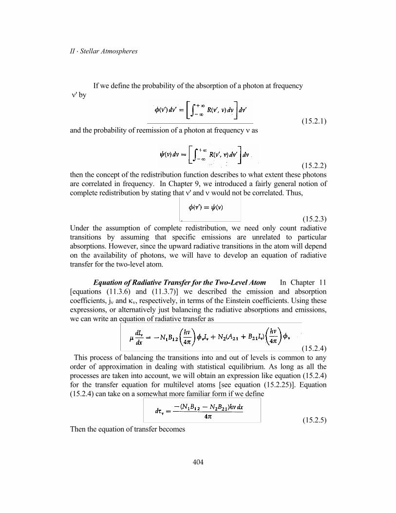
(15.2.3) Under the assumption of complete redistribution, we need only count radiative transitions by assuming that specific emissions are unrelated to particular absorptions. However, since the upward radiative transitions in the atom will depend on the availability of photons, we will have to develop an equation of radiative transfer for the two-level atom. Equation of Radiative Transfer for the Two-Level Atom In Chapter 11 [equations (11.3.6) and (11.3.7)] we described the emission and absorption coefficients, jν and κν, respectively, in terms of the Einstein coefficients. Using these expressions, or alternatively just balancing the radiative absorptions and emissions, we can write an equation of radiative transfer as

(15.2.4) This process of balancing the transitions into and out of levels is common to any order of approximation in dealing with statistical equilibrium. As long as all the processes are taken into account, we will obtain an expression like equation (15.2.4) for the transfer equation for multilevel atoms [see equation (15.2.25)]. Equation (15.2.4) can take on a somewhat more familiar form if we define

(15.2.5) Then the equation of transfer becomes

404


(15.2.6) where

(15.2.7) Making use of the relationships between the Einstein coefficients determined in Chapter 11 [equation (11.3.5)], we can further write

(15.2.8) Under conditions of LTE

(15.2.9) so that we recover the expected result for the source function, namely

(15.2.10) Two-Level-Atom Statistical Equilibrium Equations The solution to equation (15.2.6) will provide us with a value of the radiation field required to determine the number of radiative transitions. Thus the total number of upward transitions in the two-level atom is

(15.2.11) Similarly, the number of downward transitions is

(15.2.12) The requirement that the level populations be stationary means that

(15.2.13) so that the ratio of level populations is

(15.2.14)

405


Now consider a situation where there is no radiation field and the collisions are driven by particles characterized by a maxwellian energy distribution. Under these conditions, the principle of detailed balancing requires that

(15.2.15) or

(15.2.16) This argument is similar to that used to obtain the relationships between the Einstein coefficients and since the collision coefficients depend basically on atomic constants, equation (15.2.16) must hold under fairly arbitrary conditions. Specifically, the result will be unaffected by the presence of a radiation field. Thus we may use it and the relations between the Einstein coefficients [equations (11.3.5)] to write the line source function as

15.2.17) If we let

(15.2.18) then the source function takes on the more familiar form

(15.2.19) The quantity ε is, in some sense, a measure of the departure from LTE and is sometimes called the departure coefficient. A similar method for describing the departures from LTE suffered by an atom is to define

(15.2.20) where N j is the level population expected in LTE so that bj is just the ratio of the actual population to that given by the Saha-Boltzmann formula. From that definition, equation (15.2.14), and the relations among the Einstein coefficients we get

(15.2.21) 406

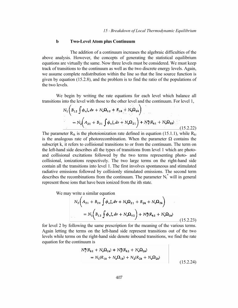
15 ⋅ Breakdown of Local Thermodynamic Equilibrium b Two-Level Atom plus Continuum The addition of a continuum increases the algebraic difficulties of the above analysis. However, the concepts of generating the statistical equilibrium equations are virtually the same. Now three levels must be considered. We must keep track of transitions to the continuum as well as the two discrete energy levels. Again, we assume complete redistribution within the line so that the line source function is given by equation (15.2.8), and the problem is to find the ratio of the populations of the two levels. We begin by writing the rate equations for each level which balance all transitions into the level with those to the other level and the continuum. For level 1,

(15.2.22) The parameter Rik is the photoionization rate defined in equation (15.1.1), while Rki is the analogous rate of photorecombination. When the parameter Ω contains the subscript k, it refers to collisional transitions to or from the continuum. The term on the left-hand side describes all the types of transitions from level 1 which are photo- and collisional excitations followed by the two terms representing photo- and collisional, ionizations respectively. The two large terms on the right-hand side contain all the transitions into level 1. The first involves spontaneous and stimulated radiative emissions followed by collisionly stimulated emissions. The second term describes the recombinations from the continuum. The parameter Ni

* will in general represent those ions that have been ionized from the ith state. We may write a similar equation

(15.2.23) for level 2 by following the same prescription for the meaning of the various terms. Again letting the terms on the left-hand side represent transitions out of the two levels while terms on the right-hand side denote inbound transitions, we find the rate equation for the continuum is

(15.2.24)

407


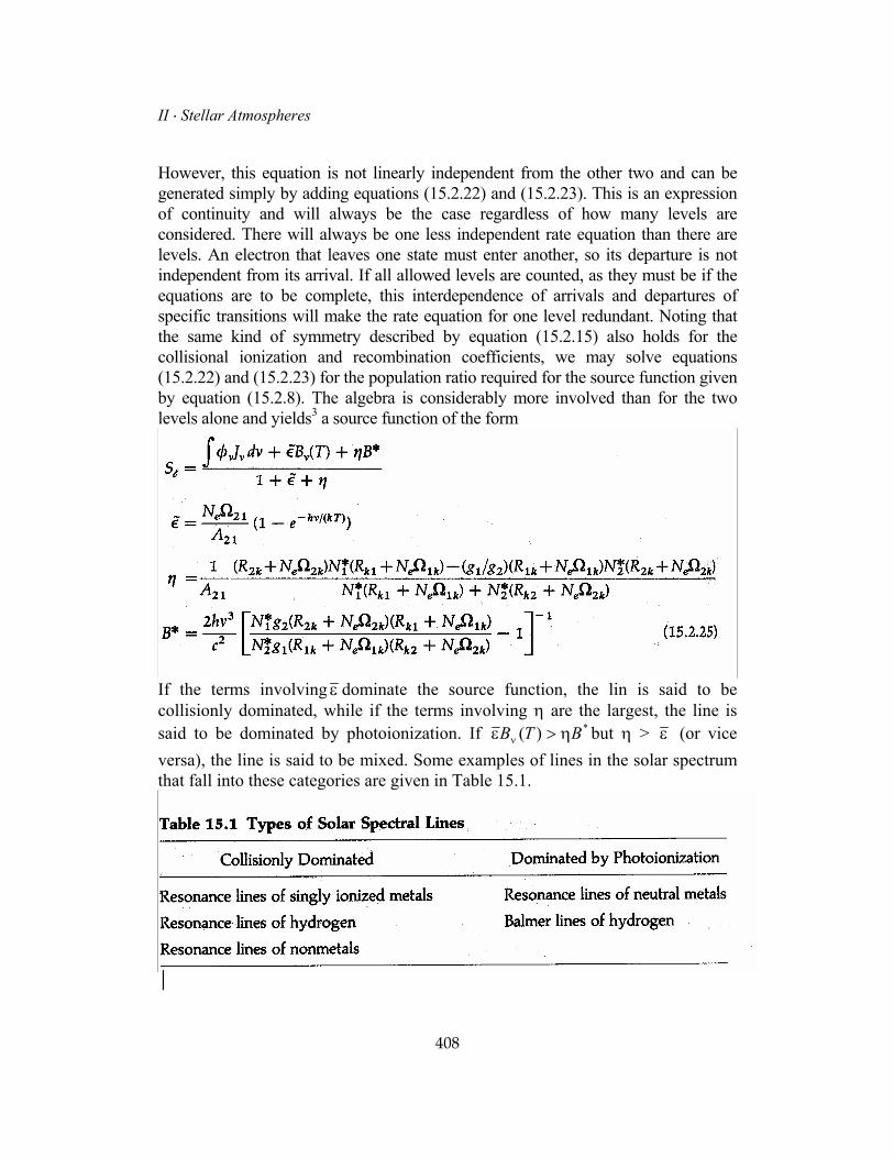
However, this equation is not linearly independent from the other two and can be generated simply by adding equations (15.2.22) and (15.2.23). This is an expression of continuity and will always be the case regardless of how many levels are considered. There will always be one less independent rate equation than there are levels. An electron that leaves one state must enter another, so its departure is not independent from its arrival. If all allowed levels are counted, as they must be if the equations are to be complete, this interdependence of arrivals and departures of specific transitions will make the rate equation for one level redundant. Noting that the same kind of symmetry described by equation (15.2.15) also holds for the collisional ionization and recombination coefficients, we may solve equations (15.2.22) and (15.2.23) for the population ratio required for the source function given by equation (15.2.8). The algebra is considerably more involved than for the two levels alone and yields3 a source function of the form

If the terms involving ε dominate the source function, the lin is said to be collisionly dominated, while if the terms involving η are the largest, the line is said to be dominated by photoionization. If *)( BTB η>ε ν but η > ε (or vice versa), the line is said to be mixed. Some examples of lines in the solar spectrum that fall into these categories are given in Table 15.1.

408

15 ⋅ Breakdown of Local Thermodynamic Equilibrium c Multilevel Atom A great deal of effort has gone into approximating the actual case of many levels of excitation by setting up and solving the rate equations for three and four levels or approximating any particular transition of interest by an "equivalent two level atom" (see D.Mihalas3, pp. 391-394). However, the advent of modern, swift computers has made most of these approximations obsolete. Instead, one considers an n-level atom (with continuum) and solves the rate equations directly. We have already indicated that this procedure can be integrated into the standard algorithm for generating a model atmosphere quite easily. Consider the generalization of equations (15.2.22) through (15.2.24). Simply writing equations for each level, by balancing the transitions into the level with those out of the level, will yield a set of equations which are linear in the level populations. However, as we have already indicated, these equations are redundant by one. So far we have only needed population ratios for the source function, but if we are to find the population levels themselves, we will need an additional constraint. The most obvious constraint is that the total number of atoms and ions must add up to the abundance specified for the atmosphere. Mihalas4 suggests using charge conservation, which is a logically equivalent constraint. Whatever additional constraint is chosen, it should be linear in the level populations so that the linear nature of the equations is not lost. It is clear that the equations are irrevocably coupled to the radiation field through the photoexcitation and ionization terms. It is this coupling that led to the rather messy expressions for the source functions of the two-level atom. However, if one takes the radiation field and electron density as known, then the rate equations have the form

(15.2.26) where A is a matrix whose elements are the coefficients multiplying the population levels and

ris a vector whose elements are the populations of the energy levels for

all species considered in the calculation. The only nonzero element of the constant vector

N

Br

arises from the additional continuity constraint that replaced the redundant level equation. These equations are fairly sparse and can be solved quickly and accurately by well-known techniques.

409

Since the standard procedure for the construction of a model atmosphere is an iterative one wherein an initial guess for the temperature distribution gives rise to the atmospheric structure, which in turn allows for the solution of the equation of radiative transfer, the solution of the rate equations can readily be included in this process. The usual procedure is to construct a model atmosphere in LTE that nearly


satisfies radiative equilibrium. At some predetermined level of accuracy, the rate equations are substituted for the Saha-Boltzmann excitation and ionization equations by using the existing structure (electron density and temperature distribution) and radiation field. The resulting population levels are then used to calculate opacities and the atmospheric structure for the next iteration. One may even chose to use an iterative algorithm for the solution of the linear equations, for an initial guess of the LTE populations will probably be quite close to the correct populations for many of the levels that are included. The number of levels of excitation that should be included is somewhat dictated by the problem of interest. Depending on the state of ionization, four levels are usually enough to provide sufficient accuracy. However, some codes routinely employ as many as eight. One criterion of use is to include as many levels as is necessary to reach those whose level populations are adequately given by the Saha-Boltzmann ionization-excitation formula. Many authors consider the model to be a non-LTE model if hydrogen alone has been treated by means of rate equations while everything else is obtained from the Saha-Boltzmann formula. For the structure of normal stellar atmospheres, this is usually sufficient. However, should specific spectral lines be of interest, one should consider whether the level populations of the element in question should also be determined from a non-LTE calculation. This decision will largely be determined by the conditions under which the line is formed. As a rule of thumb, if the line occurs in the red or infra-red spectral region, consideration should be given to a non-LTE calculation. The hotter the star, the more this consideration becomes imperative. d Thermalization Length Before we turn to the solution of the equation of radiative transfer for lines affected by non-LTE effects, we should an additional concept which helps characterize the physical processes that lead to departures from LTE. It is known as the thermalization length. In LTE all the properties of the gas are determined by the local values of the state variables. However, as soon as radiative processes become important in establishing the populations of the energy levels of the gas, the problem becomes global. Let l be the mean free path of a photon between absorptions or scatterings and ℒ be the mean free path between collisional destructions. If scatterings dominate over collisions, then ℒ will not be a "straight line" distance through the atmosphere. Indeed, ℒ >> l if Aij >> Cij. That is, if the probability of radiative de-excitation is very much greater than the probability of collisional de-excitation, then an average photon will have to travel much farther to be destroyed by a collision than by a radiative interaction. However, ℒ >> l if Cij >> Aij. In this instance, all photons that interact radiatively will be destroyed by collisions.

410

15 ⋅ Breakdown of Local Thermodynamic Equilibrium If the flow of photons is dominated by scatterings, then the character of the radiation field will be determined by photons that originate within a sphere of radius ℒ rather than l. However, ℒ should be regarded as an upper limit because many radiative interactions are pure absorptions that result in the thermalization of the photon as surely as any collisional interaction. In the case when ℒ >> l, some photons will travel a straight-line distance equal to ℒ, but not many. A better estimate for an average length traveled before the photon is thermalized would include other interactions through the notion of a "random walk". If n is the ratio of radiative to collisional interactions, then a better estimate of the thermalization length would be

(15.2.27) If the range of temperature is large over a distance corresponding to the thermalization length lth, then the local radiation field will be characterized by a temperature quite different from the local kinetic gas temperature. These departures of the radiation field from the local equilibrium temperature will ultimately force the gas out of thermodynamic equilibrium. Clearly, the greatest variation in temperature within the thermalization sphere will occur as one approaches the boundary of the atmosphere. Thus it is no surprise that these departures increase near the boundary. Let us now turn to the effects of non-LTE on the transfer of radiation. 15.3 Non-LTE Transfer of Radiation and the Redistribution Function

While we did indicate how departures of the populations of the energy levels from their LTE values could be included in the construction of a model atmosphere so that any structural effects are included, the major emphasis of the effects of non-LTE has been on the strengths and shapes of spectral lines. During the discussion of the two level atom, we saw that the form of the source function was somewhat different from what we discussed in Chapter 10. Indeed, the equation of transfer [equation (15.2.6)] for complete redistribution appears in a form somewhat different from the customary plane-parallel equation of transfer. Therefore, it should not be surprising to find that the effects of non-LTE can modify the profile of a spectral line. The extent and nature of this modification will depend on the nature of the redistribution function as well as on the magnitude of the departures from LTE. Since we already introduced the case of complete redistribution [equations (15.2.1) and (15.2.2), we begin by looking for a radiative transfer solution for the case where the emitted and absorbed photons within a spectral line are completely uncorrelated.

411


a Complete Redistribution In Chapter 14, we devoted a great deal of effort to developing expressions for the atomic absorption coefficient for spectral lines that were broadened by a number of phenomena. However, we dealt tacitly with absorption and emission processes as if no energy were exchanged with the gas between the absorption and reemission of the photon. Actually this connection was not necessary for the calculation of the atomic line absorption coefficient, but this connection is required for calculating the radiative transfer of the line radiation. Again, for the case of pure absorption there is no relationship between absorbed and emitted photons. However, in the case of scattering, as with the Schuster-Schwarzschild atmosphere, the relationship between the absorbed and reemitted photons was assumed to be perfect. That is, the scattering was assumed to be completely coherent. In a stellar atmosphere, this is rarely the case because micro-perturbations occurring between the atoms and surrounding particles will result in small exchanges of energy, so that the electron can be viewed as undergoing transitions within the broadened energy level. If those transitions are numerous during the lifetime of the excited state, then the energy of the photon that is emitted will be uncorrelated with that of the absorbed photon. In some sense the electron will "lose all memory" of the details of the transition that brought it to the excited state. The absorbed radiation will then be completely redistributed throughout the line. This is the situation that was described by equations (15.2.1) through (15.2.3), and led to the equation of transfer (15.2.6) for complete redistribution of line radiation. Although this equation has a slightly different form from what we are used to, it can be put into a familiar form by letting

(15.3.1) It now takes on the form of equation (10.1.1), and by using the classical solution discussed in Chapter 10, we can obtain an integral equation for the mean intensity in the line in terms of the source function.

(15.3.2) This can then be substituted into equation (15.2.19) to obtain an integral equation for the source function in the line.

(15.3.3)

412

15 ⋅ Breakdown of Local Thermodynamic Equilibrium The integral over x results from the integral of the mean intensity over all frequencies in the line [see equation (15.2.19)]. Note the similarity between this result and the integral equation for the source function in the case of coherent scattering [equation (9.1.14)]. Only the kernel of the integral has been modified by what is essentially a moment in frequency space weighted by the line profile function φx(t). This is clearly seen if we write the kernel as

(15.3.4) so that the source function equation becomes a Schwarzschild-Milne equation of the form

(15.3.5) Since

(15.3.6) the kernel is symmetric in τx and t, so that K(τx,t) = K(t,τx). This is the same symmetry property as the exponential integral E1τ-t in equation 10.1.14. Unfortunately, for an arbitrary depth dependence of φx(t), equations (15.3.4) and (15.3.5) must be solved numerically. Fortunately, all the methods for the solution of Schwarzschild-Milne equations discussed in Chapter 10 are applicable to the solution of this integral equation. While it is possible to obtain some insight into the behavior of the solution for the case where φx(t) ≠ f(t) (see Mihalas3, pp.366-369), the insight is of dubious value because it is the solution for a special case of a special case. However, a property of such solutions, and of noncoherent scattering in general, is that the core of the line profile is somewhat filled in at the expense of the wings. As we saw for the two-level atom with continuum, the source function takes on a more complicated form. Thus we turn to the more general situation involving partial redistribution. b Hummer Redistribution Functions The advent of swift computers has made it practical to model the more complete description of the redistribution of photons in spectral lines. However, the attempts to describe this phenomenon quantitatively go back to L.Henyey5 who carried out detailed balancing within an energy level to describe the way in which photons are actually redistributed across a spectral line. Unfortunately, the computing power of the time was not up to the task, and this approach to the problem has gone virtually unnoticed. More recently, D.Hummer6 has classified the problem of redistribution into four main categories which are widely used today. For 413


these cases, the energy levels are characterized by Lorentz profiles which are appropriate for a wide range of lines. Regrettably, for the strong lines of hydrogen, many helium lines as well as most strong resonance lines, this characterization is inappropriate (see Chapter 14) and an entirely different analysis must be undertaken. This remains one of the current nagging problems of stellar astrophysics. However, the Hummer classification and analysis provides considerable insight into the problems of partial redistribution and enables rather complete analyses of many lines with Lorentz profiles produced by the impact phase-shift theory of collisional broadening. Let us begin the discussion of the Hummer redistribution functions with a few definitions. Let p(ξ', ξ)dξ be the probability that an absorbed photon having frequency ξ' is scattered into the frequency interval ξ→ ξ+ dξ. Furthermore, let the probability density function p(ξ', ξ) be normalized so that ∫p(ξ', ξ) dξ' = 1. That is, the absorbed photon must go somewhere. If this is not an appropriate result for the description of some lines, the probability of scattering can be absorbed in the scattering coefficient (see Section 9.2). In addition, let g(n',n ) be the probability density function describing scattering from a direction n ' into n , also normalized so that the integral over all solid angles, [∫g(n', n) dΩ]/(4π) = 1. For isotropic scattering, g(n',n ) = 1, while in the case of Rayleigh Scattering g(n', n ) = 3[1 + (n'⋅n)2]/4. We further define f(ξ') dξ' as the relative [that is, ∫ f (ξ') dξ' = 1 ] probability that a photon with frequency ξ' is absorbed. These probability density functions can be used to describe the redistribution function introduced in Chapter 9. In choosing to represent the redistribution function in this manner, it is tacitly assumed that the redistribution of photons in frequency is independent of the direction of scattering. This is clearly not the case for atoms in motion, but for an observer located in the rest frame of the atom it is usually a reasonable assumption. The problem of Doppler shifts is largely geometry and can be handled separately. Thus, the probability that a photon will be absorbed at frequency ξ' and reemitted at a frequency ξ is

(15.3.7) David Hummer6 has considered a number of cases where f, p, and g, take on special values which characterize the energy levels and represent common conditions that are satisfied by many atomic lines. Emission and Absorption Probability Density Functions for the Four Cases Considered by Hummer Consider first the case of coherent scattering where both energy levels are infinitely sharp. Then the absorption and reemission probability density functions will be given by

414


(15.3.8) If the lower level is broadened by collisional radiation damping but the upper level remains sharp, then the absorption probability density function is a Lorentz profile while the reemission probability density function remains a delta function, so that

15.3.9) If the lower level is sharp but the upper level is broadened by collisional radiation damping, then both probability density functions are given Lorentz profiles since the transitions into and out of the upper level are from a broadened state. Thus,

(15.3.10) Since ξ' and ξ are uncorrelated, this case represents a case of complete redistribution of noncoherent scattering. Hummer gives the joint probability of transitions from a broadened lower level to a broadened upper level and back again as

(15.3.11) This probability must be calculated as a unit since ξ' is the same for both f and p. Unfortunately a careful analysis of this function shows that the lower level is considered to be sharp for the reemitted photon and therefore is inconsistent with the assumption made about the absorption. Therefore, it will not satisfy detailed balancing in an environment that presupposes LTE. A correct quantum mechanical analysis7 gives

415


(15.3.12)

A little inspection of this rather messy result shows that it is symmetric in ξ' and ξ, which it must be if it is to obey detailed balancing. In addition, the function has two relative maxima at ξ' = ξ and ξ' = ν0. Since the center of the two energy levels represent a very likely transition, transitions from the middle of the lower level and back again will be quite common. Under these conditions ξ' = ξ and the scattering is fully coherent. On the other hand, transitions from the exact center of the lower level (ξ' = ν0) will also be very common. However, the return transition can be to any place in the lower level with frequency ξ. Since the function is symmetric in ξ' and ξ, the reverse process can also happen. Both these processes are fully noncoherent so that the relative maxima occur for the cases of fully coherent and noncoherent scattering with the partially coherent photons being represented by the remainder of the joint probability distribution function. Effects of Doppler Motion on the Redistribution Functions Consider an atom in motion relative to some fixed reference frame with a velocity r . If a photon has a frequency ξ' as seen by the atom, the corresponding frequency in the rest frame is

v

(15.3.13) Similarly, the photon emitted by the atom will be seen in the rest frame, Doppler-shifted from its atomic value by

(15.3.14) Thus the redistribution function that is seen by an observer in the rest frame is

(15.3.15) 416

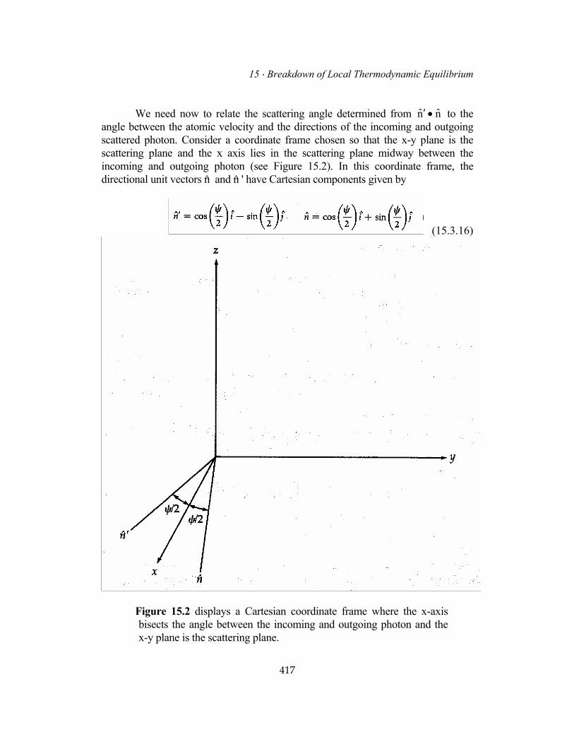
15 ⋅ Breakdown of Local Thermodynamic Equilibrium We need now to relate the scattering angle determined from to the angle between the atomic velocity and the directions of the incoming and outgoing scattered photon. Consider a coordinate frame chosen so that the x-y plane is the scattering plane and the x axis lies in the scattering plane midway between the incoming and outgoing photon (see Figure 15.2). In this coordinate frame, the directional unit vectors n and n ' have Cartesian components given by

nn •′

(15.3.16)

Figure 15.2 displays a Cartesian coordinate frame where the x-axis bisects the angle between the incoming and outgoing photon and the x-y plane is the scattering plane.

417


Now if we assume that the atoms have a maxwellian velocity distribution

(15.3.17) we can obtain the behavior of an ensemble of atoms by averaging equation (15.3.15) over all velocity. First it is convenient to make the variable transformations

(15.3.18) so that the components of the particle's velocity projected along the directions of the photon's path become

(15.3.19) and the velocity distribution is

(15.3.20) The symbol means duudr xduyduz. We define the ensemble average over the velocity of the redistribution function as

(15.3.21) or

(15.3.22) A coordinate rotation by y/2 about the y axis so that n ' is aligned with x (see Figure 15.2) leads to the equivalent, but useful, form

418


(15.3.23) We are now in a position to evaluate the effects of thermal Doppler motion on the four cases given by Hummer6, represented by equations (15.3.8) through (15.3.12). The substitution of these forms of f(ξ') and p(ξ', ξ) into equation (15.3.22) or equation (15.3.23) will yield the desired result. The frequencies ξ' and ξ must be Doppler shifted according to equations (15.3.13) and (15.3.14) and some difficulty may be encountered for the case of direct forward or back scattering (that is, β = 0) and when one of the distribution functions is a delta function (i.e., for a sharp energy level). The fact that β = 0 for these cases should be invoked before any variable transformations are made for the purposes of evaluating the integrals. Making a final transformation to a set of dimensionless frequencies

(15.3.24) we can obtain the following result for Hummer's case I:

(15.3.25) Consider what the emitted radiation would look like for an ensemble of atoms illuminated by an isotropic uniform radiation field I0. Substitution of such a radiation field into equation (9.2.29) would yield

(15.3.26) which after some algebra gives

(15.3.27) This implies that the emission of the radiation would have exactly the same form as the absorption profile. But this was our definition of complete redistribution [see equation (15.2.3)]. Thus, although a single atom behaves coherently, an ensemble of thermally moving atoms will produce a line profile that is equivalent to one suffering complete redistribution of the radiation over the Doppler core. Perhaps this is not too surprising since the motion of the atoms is totally uncorrelated so that the Doppler shifts produced by the various motions will mimic complete redistribution. 419


As one proceeds with the progressively more complicated cases, the results become correspondingly more complicated to derive and express. Hummer's cases II and III yield

(15.3.28) and

(15.3.29) respectively. There is little point in giving the result for case IV as given by equation (15.3.11). But the result for the correct case IV (sometimes called case V) that is obtained from equation (15.3.12) is of some interest and is given by McKenna8 as

(15.3.30) where

(15.3.31) and the function K(a,x), which is known as the shifted Voigt function is defined by

(15.3.32)

420

15 ⋅ Breakdown of Local Thermodynamic Equilibrium Unfortunately, all these redistribution functions contain the scattering angle ψ explicitly and so by themselves are difficult to use for the calculation of line profiles. Not only does the scattering angle appear in the part of the redistribution function resulting from the effects of the Doppler motion, but also the scattering angle is contained in the phase function g(n', ). Thus, the Doppler motion can be viewed as merely complicating the phase function. While there are methods for dealing with the angle dependence of the redistribution function (see McKenna

n

9), they are difficult and beyond the present scope of this discussion. They are, however, of considerable importance to those interested in the state of polarization of the line radiation. For most cases, the phase function is assumed to be isotropic, and we may remove the angle dependence introduced by the Doppler motion by averaging the redistribution function over all angles, as we did with velocity. These averaged forms for the redistribution functions can then be inserted directly into the equation of radiative transfer. As long as the radiation field is nearly isotropic and the angular scattering dependence (phase function) is also isotropic, this approximation is quite accurate. However, always remember that it is indeed an approximation. Angle-Averaged Redistribution Functions We should remember from Chapter 13 [equation (13.2.14)], and the meaning of the redistribution function [see equation (9.2.29)], that the equation of transfer for line radiation can be written as

(15.3.33) Here the parameter ℒν is not to be considered constant with depth as it was for the Milne-Eddington atmosphere. If we assume that the radiation field is nearly isotropic, then we can integrate the equation of radiative transfer over µ and write

(15.3.34) If we define the angle-averaged redistribution function as

(15.3.35) then in terms of the absorption and reemission probabilities f(ξ') and p(ξ', ξ) it becomes

(15.3.36) 421


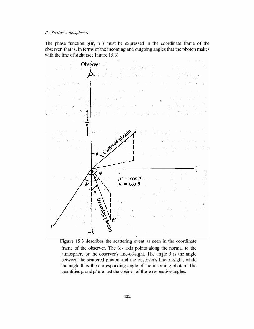
The phase function g(n', n ) must be expressed in the coordinate frame of the observer, that is, in terms of the incoming and outgoing angles that the photon makes with the line of sight (see Figure 15.3).

Figure 15.3 describes the scattering event as seen in the coordinate frame of the observer. The k - axis points along the normal to the atmosphere or the observer's line-of-sight. The angle θ is the angle between the scattered photon and the observer's line-of-sight, while the angle θ' is the corresponding angle of the incoming photon. The quantities µ and µ' are just the cosines of these respective angles.

ˆ

422

15 ⋅ Breakdown of Local Thermodynamic Equilibrium We may write the phase function g(n', n ) as

(15.3.37) so that the angle-averaged redistribution function becomes

(15.3.38) The two most common types of phase functions are isotropic scattering and Rayleigh scattering. Although the latter occurs more frequently in nature, the former is used more often because of its simplicity. Evaluating these phase functions in terms of the observer's coordinate frame yields

(15.3.39) In general, the appropriate procedure for calculating the angle-averaged redistribution functions involves carrying out the integrals in equation (15.3.38) and then applying the effects of Doppler broadening so as to obtain a redistribution function for the four cases described by Hummer. For the first two cases, the delta function representing the upper and lower levels requires that some care be used in the evaluation of the integrals (see Mihalas4, pp. 422-433). In terms of the normalized frequency x, the results of all that algebra are, for case I

(15.3.40) For case II the result is somewhat more complicated where

(15.3.41) while for case III it is more complex still:

(15.3.42) Note that for all these cases the redistribution function is symmetric in x and x'. From equations (15.2.1) through (15.2.3), it is clear that the angle-averaged

423


redistribution functions will yield a complete redistribution profile in spite of the fact that case I is completely coherent. To demonstrate the effect introduced by an anisotropic phase function, we give the results for redistribution by electrons. Although we have always considered electron scattering to be fully coherent in the atom's coordinate frame, the effect of Doppler motion can introduce frequency shifts that will broaden a spectral line. This is a negligible effect when we are calculating the flow of radiation in the continuum, but it can introduce significant broadening of spectral lines. If we assume that the scattering function for electrons is isotropic, then the appropriate angle-averaged redistribution function has the form

(15.3.43) However, the correct phase function for electron scattering is the Rayleigh phase function given in the observer's coordinate frame by the second of equations (15.3.39). The angle-averaged redistribution function for this case has been computed by Hummer and Mihalas10 and is

Clearly the use of the correct phase function causes a significant increase in the complexity of the angle-averaged redistribution function. Since the angle-averaged redistribution function itself represents an approximation requiring an isotropic radiation field, one cannot help but wonder if the effort is justified. We must also remember that the entire discussion of the four Hummer cases relied on the absorption and reemission profiles being given by Lorentz profiles in the more complicated cases. While considerable effort has been put into calculating the Voigt functions and functions related to them that arise in the generation of the redistribution functions11, some of the most interesting lines in stellar astrophysics are poorly described by Lorentz profiles. Perhaps the most notable example is the lines of hydrogen. At present, there is no quantitative representation of the redistribution function for any of the hydrogen lines. While noncoherent scattering is probably appropriate for the cores of these lines, it most certainly is not for the wings. Since a great deal of astrophysical information rests on matching theoretical line profiles of the Balmer lines to those of stars, greater effort should be made on the correct modeling of these lines, including the appropriate redistribution functions. The situation is even worse when one tries to estimate the polarization to be expected within a spectral line. It is a common myth in astrophysics that the radiation

424

15 ⋅ Breakdown of Local Thermodynamic Equilibrium in a spectral line should be locally unpolarized. Hence, the global observation of spectral lines should show no net polarization. While this is true for simple lines that result only from pure absorption, it is not true for lines that result from resonant scattering. The phase function for a line undergoing resonant scattering is essentially the same as that for electron scattering - the Rayleigh phase function. While noncoherent scattering processes will tend to destroy the polarization information, those parts of the line not subject to complete redistribution will produce strong local polarization. If the source of the radiation does not exhibit symmetry about the line of sight, then the sum of the local net polarization will not average to zero as seen by the observer. Thus there should be a very strong wavelength polarization through such a line which, while difficult to model, has the potential of placing very tight constraints on the nature of the source. Recently McKenna12 has shown that this polarization, known to exist in the specific intensity profiles of the sun, can be successfully modeled by proper treatment of the redistribution function and a careful analysis of the transfer of polarized radiation. So it is clear that the opportunity is there remaining to be exploited. The existence of modern computers now makes this feasible. 15.4 Line Blanketing and Its Inclusion in the Construction of Model Stellar Atmospheres and Its Inclusion in the Construction of Model Stellar Atmospheres

In Chapter 10, we indicated that the presence of myriads of weak spectral lines could add significantly to the total opacity in certain parts of the spectrum and virtually blanket the emerging flux forcing it to appear in other less opaque regions of the spectrum. This is particularly true for the early-type stars for which the major contribution from these lines occurs in the ultraviolet part of the spectrum, where most of the radiative flux flows from the atmosphere. Although it is not strictly a non-LTE effect, the existence of these lines generally formed high in the atmosphere can result in structural changes to the atmosphere not unlike those of non-LTE. The addition of opacity high up in the atmosphere tends to heat the layers immediately below and is sometimes called backwarming.

425

Because of their sheer number, the inclusion of these lines in the calculation of the opacity coefficient poses some significant problems. The simple approach of including sufficient frequency points to represent the presence of all these lines would simply make the computational problem unmanageable with even the largest of computing machines that exist or can be imagined. Since the early attempts of Chandrasekhar13, many efforts have been made to include these effects in the modeling of stellar atmospheres. These early efforts incorporated approximating the lines by a series of frequency "pickets". That is, the frequency dependence would be represented by a discontinuous series of opaque regions that alternate with transparent regions. One could then average over larger sections of the spectrum to obtain a mean line opacity for the entire region. However, this did not represent the


effect on the photon flow through the alternatingly opaque and relatively transparent regions with any great accuracy. Others tried using harmonic mean line opacities to reduce this problem. Of these attempts, two have survived and are worthy of consideration. a Opacity Sampling This conceptually simple method of including line blanketing takes advantage of the extremely large number of spectral lines. The basic approach is to represent the frequency-dependent opacity of all the lines as completely as possible. This requires tabulating a list of all the likely lines and their relative strengths. For an element like iron, this could mean the systematic listing of several million lines. In addition, the line shape for each line must be known. This is usually taken to be a Voigt function for it represents an excellent approximation for the vast majority of weak lines. However, its use requires that some estimate of the appropriate damping constant be obtained for each line. In many cases, the Voigt function has been approximated by the Doppler broadening function on the assumption that the damping wings of the line are relatively unimportant. At any frequency the total line absorption coefficient is simply the sum of the significant contributions of lines that contribute to the opacity at that frequency, weighted by the relative abundance of the absorbing species. These abundances are usually obtained by assuming that LTE prevails and so the Saha-Boltzmann ionization-excitation equation can be used. If one were to pick a very large number of frequencies, this procedure would yield an accurate representation of the effects of metallic line blanketing. However, it would also require prodigious quantities of computing time for modeling the atmosphere. Sneden et al.14 have shown that sufficient accuracy can be obtained by choosing far fewer frequency points than would be required to represent each line accurately. Although the choice of randomly distributed frequency points which represent large chunks of the frequency domain means that the opacity will be seriously overestimated in some regions and underestimated in others, it is possible to obtain accurate structural results for the atmosphere if a large enough sample of frequency points is chosen. This sample need not be anywhere near as large as that required to represent the individual lines, for what is important for the structure is only the net flow of photons. Thus, if the frequency sampling is sufficiently large to describe the photon flow over reasonably large parts of the spectrum, the resulting structure and the contribution of millions of lines will be accurately represented. This procedure will begin to fail in the higher regions of the atmosphere where the lines become very sharp and non-LTE effects become increasingly important. In practice, this procedure may require the use of several thousand frequency points whereas the correct representation of several million spectral lines would require tens of millions of frequency points. For this reason (and others), this approach has been extremely successful as applied to the structure of late-type model atmospheres where the

426

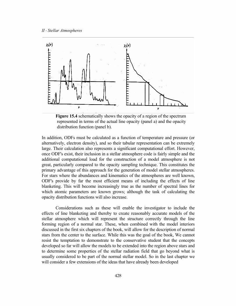
15 ⋅ Breakdown of Local Thermodynamic Equilibrium opacity is dominated by the literally millions of bound-bound transitions occurring in molecules. The larger the number of weak lines and the more uniform their distribution, the more accurate this procedure becomes. However, the longer the lists of spectral lines, the more computer time will be required to carry out the calculation. This entire procedure is generally known as opacity sampling and it possesses a great degree of flexibility in that all aspects of the stellar model that may affect the line broadening can be included ab initio for each model. This is not the case with the competing approach to line blanketing. b Opacity Distribution Functions This approach to describing the absorption by large numbers of lines also involves a form of statistical sampling. However, here the statistical representation is carried out over even larger regions of the spectra than was the case for the opacity sampling scheme. This approach has its origins in the mean opacity concept alluded to earlier. However, instead of replacing the complicated variation of the line opacity over some region of the spectrum with its mean, consider the fraction of the spectral range that has a line opacity less than or equal to some given value. For small intervals of the range, this may be a fairly large number since small intervals correspond to the presence of line cores. If one considers larger fractions of the interval, the total opacity per unit frequency interval of this larger region will decrease, because the spaces between the lines will be included. Thus, an opacity distribution function represents the probability that a randomly chosen point in the interval will have an opacity less than or equal to the given value (see Figure 15.4). The proper name for this function should be the inverse cumulative opacity probability distribution function, but in astronomy it is usually referred to as just the opacity distribution function or (ODF). Carpenter15 gives a very complete description of the details of computing these functions while a somewhat less complete picture is given by Kurucz and Pettymann16and by Mihalas 4(pp. 167-169). The ODF gives the probability that the opacity is a particular fraction of a known value for any range of the frequency interval, and the ODF may be obtained from a graph that is fairly simple to characterize by simple functions. This approach allows the contribution to the total opacity due to spectral lines appropriate for that range of the interval to be calculated. Unfortunately, the magnitude of that given value will depend on the chemical composition and the details of the individual line-broadening mechanisms. Thus, any change in the chemical composition, turbulent broadening, etc., will require a recalculation of the ODF.

427


Figure 15.4 schematically shows the opacity of a region of the spectrum represented in terms of the actual line opacity (panel a) and the opacity distribution function (panel b).

In addition, ODFs must be calculated as a function of temperature and pressure (or alternatively, electron density), and so their tabular representation can be extremely large. Their calculation also represents a significant computational effort. However, once ODF's exist, their inclusion in a stellar atmosphere code is fairly simple and the additional computational load for the construction of a model atmosphere is not great, particularly compared to the opacity sampling technique. This constitutes the primary advantage of this approach for the generation of model stellar atmospheres. For stars where the abundances and kinematics of the atmospheres are well known, ODF's provide by far the most efficient means of including the effects of line blanketing. This will become increasingly true as the number of spectral lines for which atomic parameters are known grows; although the task of calculating the opacity distribution functions will also increase. Considerations such as these will enable the investigator to include the effects of line blanketing and thereby to create reasonably accurate models of the stellar atmosphere which will represent the structure correctly through the line forming region of a normal star. These, when combined with the model interiors discussed in the first six chapters of the book, will allow for the description of normal stars from the center to the surface. While this was the goal of the book, We cannot resist the temptation to demonstrate to the conservative student that the concepts developed so far will allow the models to be extended into the region above stars and to determine some properties of the stellar radiation field that go beyond what is usually considered to be part of the normal stellar model. So in the last chapter we will consider a few extensions of the ideas that have already been developed

428

15 ⋅ Breakdown of Local Thermodynamic Equilibrium Problems 1. Estimate the ratio of collisional ionization to photoionization for hydrogen

from the ground state, and compare it to the ratio from the second level. Assume the pressure is 300 bars. Obtain the physical constants you may need from the literature, but give the appropriate references.

2. Calculate the Doppler-broadened angle-averaged redistribution function for Hummer's case I, but assuming a Rayleigh phase function [i.e., find <R(x,x')>I,B] and compare it to <R(x,x')>I,A and the result for electron scattering.

3. Show that

is indeed a solution to

and obtain an integral equation for Sl. 4. Describe the mechanisms which determine the Lyα profile in the sun. Be

specific about the relative importance of these mechanisms and the parts of the profile that they affect.

5. Given a line profile of the form

find Sl. Assume complete redistribution of the line radiation. State what further assumptions you may need; indicate your method of solution and your reasons for choosing it.

6. Show explicitly how equation (15.2.21) is obtained. 7. Show how equation (15.3.25) is implied by equation (15.3.15). 8. How does equation (15.3.27) follow from equation (15.3.26). 9. Derive equations (15.3.28) and (15.3.29). 10. Use equation (15.3.30) to obtain the angle-averaged form of <RIV,A(x',x)>. 11. Show explicitly how equations (15.3.40) and (15.3.41) are obtained. 429


References and Supplemental Reading 1. Woolley, R.v.d.R., and Stibbs, D.W.N. The Outer Layers of a Star, Oxford University Press, London, 1953, p. 152. 2. Böhm, K.-H. "Basic Theory of Line Formation", Stellar Atmospheres, (Ed.:

J. Greenstein), Stars and Stellar Systems: Compendium of Astronomy and Astrophysics, Vol.6, University of Chicago Press, 1960, pp. 88 - 155.

3. Mihalas, D. Stellar Atmospheres, W.H. Freeman, San Francisco, 1970, pp. 337 - 378. 4. Mihalas, D. Stellar Atmospheres, 2d ed., W.H. Freeman, San Francisco,

1978, pp. 138. 5. Henyey, L. Near Thermodynamic Radiative Equilibrium, Ap.J. 103, 1946,

pp. 332 - 350. 6. Hummer, D.G. Non-Coherent Scattering, Mon. Not. R. astr. Soc. 125, 1962,

pp. 21 - 37. 7. Omont, A., Smith, E.R., and Cooper, J. Redistribution of Resonance

Radiation I. The Effect of Collisions, Ap.J. 175, 1972, pp. 185 - 199. 8. McKenna,S. A Reinvestigation of Redistribution Functions RIII and RIV, Ap.

J. 175, 1980, pp. 283 - 293. 9. McKenna, S. The Transfer of Polarized Radiation in Spectral

Lines:Formalism and Solutions in Simple Cases, Astrophy. & Sp. Sci., 108, 1985, pp. 31 - 66.

10. Hummer, D.G., and Mihalas, D. Line Formation with Non-Coherent

Electron Scattering in O and B Stars, Ap.J. Lett. 150, 1967, pp. 57 - 59. 11. McKenna, S. A Method of Computing the Complex Probability Functionand

Other Related Functions over the Whole Complex Plane, Astrophy. & Sp. Sci. 107, 1984, pp. 71 - 83.

12. McKenna, S. The Transfer of Polarized Radiation in Spectral Lines: Solar-

Type Stellar Atmospheres, Astrophy. & Sp. Sci., 106, 1984, pp. 283 - 297. 430


431

13. Chandrasekhar,S. The Radiative Equilibrium of the Outer Layers of a Star with Special Reference to the Blanketing Effect of the Reversing Layer, Mon. Not. R. astr. Soc. 96, 1936, pp. 21 - 42.

14. Sneden, C., Johnson, H.R., and Krupp, B.M. A Statistical Method for

Treating Molecular Line Opacities, Ap. J. 204, 1976, pp. 281 - 289. 15. Carpenter,K.G. A Study of Magnetic, Line-Blanketed Model Atmospheres,

doctoral dissertation: The Ohio State University, Columbus, 1983. 16. Kurucz, R., and Peytremann, E. A Table of Semiemperical gf Values Part 3,

SAO Special Report #362, 1975. Although they have been cited frequently, the serious student of departures from LTE should read both these: Mihalas, D.: Stellar Atmospheres, W.H.Freeman, San Francisco, 1970, chaps. 7-10, 12, 13. and Mihalas, D.: Stellar Atmospheres, 2d ed., W.H.Freeman, San Francisco,

1978, chaps. 11-13. A somewhat different perspective on the two-level and multilevel atom can be found in: Jefferies, J.T.: Spectral Line Formation, Blaisdell, New York, 1968, chaps. 7, 8. Although the reference is somewhat old, the physical content is such that I would still recommend reading the entire chapter: Böhm, K.-H.: "Basic Theory of Line Formation", Stellar Atmospheres, (Ed.:

J.Greenstein), Stars and Stellar Systems: Compendium of Astronomy and Astrophysics, Vol.6, University of Chicago Press, Chicago, 1960, chap. 3.

Documents

15 Breakdown of Local Thermodynamic Equilibriumads.harvard.edu/books/1989fsa..book/AbookC15.pdf · II ⋅ Stellar Atmospheres 15.1 Phenomena Which Produce Departures from Local Thermodynamic