12978 Surjit Bhalla Two Policy Briefs

8/2/2019 12978 Surjit Bhalla Two Policy Briefs

http://slidepdf.com/reader/full/12978-surjit-bhalla-two-policy-briefs 1/29

Imagine There’s No Country: Poverty, Inequality and Growth in the Era of Globalization

By

Surjit S. Bhalla*

Published by the Institute for International Economics ,September 26, 2002

Enclosed are Two Policy Briefs based on the findings of the book:

Has Growth Been Pro-Poor in the era of Globalization? 1-16

Who has Lost out to Globalization? 17-27

References 28

* Managing Director, Oxus Research & Investments, B-189 Greater Kailash – I,New Delhi 110048, India • Email: [email protected]

mailto:[email protected]

mailto:[email protected]



Policy Brief: Has Growth Been Pro-Poor in the era of Globalization?

Abstracted from Imagine There’s No Country: Poverty, Inequality and Growth in the era of Globalization , by Surjit S. Bhalla. Published by the Institute for International Economics, September 2002

1. Introduction & Overview

Does growth benefit the poor? This vital question assumes added importance in this new

era of globalization, which, some have claimed, has benefited the rich at the expense of

the poor. The success or failure of globalization depends, ultimately, not on whether

individual countries benefit but rather – and how – individuals benefit from this process.In addition to the problem of individuals versus countries, the discussion about the

nature or “quality” of growth (i.e., has growth been pro-poor?) has been marred by

problems of definition and measurement. New results, presented in Imagine there’s no

country: Poverty, inequality and Growth in the era of Globalization go a long way in

addressing these issues, and find that growth has, indeed, been resoundingly pro-poor

during the 1980s and 1990s.

The distribution of benefits from growth between countries raises the issue of individualsversus countries. Whether growth – on a regional or global level – has been pro-poor or

not depends on whether it has disproportionately (and positively) impacted poor

individuals ; this matters more than the country of origin of these individuals. Thus, if

growth has benefited 90 percent of the world’s poor, but has done so in only 10 percent

of the world’s countries, it would be correct to regard this as being pro-poor. In other

words, if poor people in China and India (who have historically constituted a vast

majority of the world’s poor) have gained from growth, the fact that poor people in some

other country (say, Ethiopia) have not gained does not indicate that growth has not beenpro-poor. This conclusion is independent of the possibility that the poor in Ethiopia have

not gained because there has not been much growth for anybody to share.

1



2. Measuring Growth, Inequality and Poverty: The Simple Accounting Procedure

The results presented in Imagine … are derived from an important methodological

advancement that makes possible the conversion of quintile distribution data on

expenditures and/or incomes, into percentile data and, further, the pooling of individual

country data to obtain regional or world distributions. While several questions can be

answered with existing data sets, this conversion allows analysis at a more

disaggregated level, which is absolutely necessary for answering the most important

questions pertaining to levels and trend in individual inequality, and levels and trends in

absolute poverty. Why is this the case? Because distribution data are not available at a

more disaggregated level than quintiles; the best that is possible is quintile data, and

even that too for a few countries, and also too aggregated for countries like China where

250 million people (20 percent) are being attributed the same level of average quintile

income.

What is required is a more disaggregated estimate of intra-country expenditures e.g. a

percentile distribution for each country-year distribution. This method would attribute the

same income to only 12.5 million in China, and the same income to each 2.8 million

people in the US, and the same income to each 600,000 people in the United Kingdom.

Towards this end, the Simple Accounting Procedure (SAP) of estimating Lorenz curve

distributions was developed, a procedure which yields 100 percentiles1 and therefore

means for 100 different and equal (in size) sets of individuals for each distribution year.

The difference between SAP and world inequality distributions developed by Berry et. al

(1983), Bourguignon-Morrisson (1999), Milanovic (1999), and Imagine … (first estimate

in June 2000, Bhalla(2000c)) - is that the first three do not construct such detailed

distributions of income2. The Bourguignon-Morrisson method has an average of 11

means per distribution and Milanovic’s combination of rural and urban data for some

Notes:

1The developed method allows even greater fine-tuning e.g. a 200 or 400 point distribution.

However, the gains from further disaggregation are probably not that great. Such increasedprecision is unlikely to change the mean income at each percentile level.2

In a very recent paper, May 2002, Sala-I-Martin also constructs a world income distribution butexaggerates when he contends that “ to our knowledge, this is the first attempt to construct aworld income distribution by aggregating individual country distribution” (p.2). That credit shouldrightfully go to the pioneering work of Berry et. al. in 1983, a work also cited by Sala-I-Martin.

2



countries yields an average of around 12 different “means” per country year. The SAP

method, moreover, is shown to be extremely accurate in “reproducing” percentile means

based on unit level data, as well as in reproducing broad indices of inequality like the

Gini.

3. The Growth-Poverty Connection

The key to understanding whether the growth process is operating in a neutral manner is

whether the poor participate “evenly” in the growth process; and evenly is defined as the

elasticity of the incomes of the poor with respect to average growth. If poverty is now

defined by not the level of the incomes of the poor, but by the proportion of population

with incomes below a specific level P (the poverty line), the answer becomes more

complex, not least because now there is a non-linear cumulative distribution function

(relating the proportion of population that is poor, the head-count ratio, HCR, to income

Y) involved. HCR now is censored above at 100 and below at 0 i.e. it ranges between no

poor (HCR equal to 0 percent) to the entire population poor (HCR equal to 100 percent).

With HCR as the variable in question, how can one determine if the growth process has

been “even” or “neutral” (“equivalent” to an elasticity equal to 1 in the incomes of the

poor model), pro-poor (equivalent to an elasticity greater than 1) or pro-rich (equivalent

to elasticity less than 1)?

Since we are talking about income poverty, the relationship should be “exhaustive” i.e.

the entire growth in income should be accounted for. By definition, changes in HCR are

equal to the sum of changes caused by incomes going up (holding the distribution of

income, I = F(Y) constant) and the changes caused by the distribution of income

changing, holding the level of income constant. In terms of first differences in logs, one

obtains,

)log(*)log(*)log( ld yd HCRd β α += (Equation 1)

Where, by definition, (α + β )=13

3

Ravallion-Datt introduce an error here; they suggest that there is a third “residual” term inequation 10.1, when conceptually there isn’t one. Kakwani(1997) correctly argues that there is no

3



This equation has been estimated by several authors, and while intuitive, it yields the

wrong answers; it is, in fact, impossible to accurately determine the percentage change

in the HCR from the above model. Several authors argue, incorrectly, that the ratio of α

to (α + β ) is indicative of whether the nature of growth is pro-poor, since the shape of the

distribution elasticity (a concept elaborated on below) plays an important role in

translating (or not translating) growth into poverty reduction.

4. Pro-poor Elasticity – With growth it can be infinite, with growth it can be zero

The most prevalent result using the wrong model (Equation 1) is that the pro-poor

elasticity, (ratio of α to (α + β )) this elasticity varies between 1.5 to 3, with the mode

around 24. It is not clear, however, as to what meaning one should attach to this

estimated elasticity. What the model states is that for each 10 percent increase in

incomes, HCR is expected to decline by 20 percent (elasticity of 2). This may seem

large, and indicative of the growth process being massively pro-poor. But, of course, the

elasticity, whatever its magnitude, is silent on the important question of whether the

growth process is pro-poor. Left unanswered is the question of how much should HCR

have declined by if the growth was “neutral” i.e. one unaccompanied by any change in

inequality.

The dependent variable is a percentage change in a ratio. If the initial value of the HCR

was 30, then a decline of 20 percent is equivalent to a decrease of only six percentage

points. Thus, a 10 percent increase in incomes in this example will lead to a 6

percentage point decline in the head-count ratio. But what should have happened? An 8

percent decline, a 10 percent, or perhaps 4 percent? We do not know, unless we know

the shape of the distribution elasticity.

The problem is caused by the fact that coefficient α in the above equation is a function of

the poverty line P . The problems this can cause for estimation is explained in heuristic

terms as follows. Assume the maximum income of the poor in a society is $0.5 per

capita per day, and the poverty line P is double this amount at $ 1. Now if all incomes go

residual. The problem with both interpretations is that they are defining the left hand side in logfirst difference terms, rather than arithmetic first difference terms. See below.4

See Collier-Dollar, Kakwani, Ravallion.

4



up by 10 percent, there will obviously be no decline in the HCR from 100 percent; the

maximum income goes up to 0.55, still far below the poverty line, P. So the elasticity of

HCR with respect to income growth (α in equation 1) is zero. Now assume that the mean

(not maximum) income of the poor is 0.5, and that the standard deviation of the incomes

of the poor is 0.1. Again a 10 percent increase in income will not make any dent in the

HCR i.e. the elasticity is zero. Now assume that all the poor have an income equal to

0.99. A 1.1 percent increase in income will now mean that the HCR will move from 100

percent to zero percent in one fell swoop; close to an infinite elasticity, or a equal to

infinity.

The above are unrealistic, but informative, examples. What they all point to is the

importance of incorporating into the calculations the knowledge of where the mean

income of the poor, and the nature of its distribution, is with respect to the poverty line,

P. This is a non-linear affair, which perhaps is one reason analysts have not attempted

to compute it.

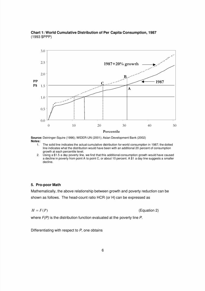
Chart 1 shows the cumulative distribution for the developing world for 1987, as well as

the same distribution “shocked” with a 20 percent across the board increase. An

increase in income of 20 percent will involve a movement from point A to point B; the

difference in the head count ratios is given by the movement from A to C. The

calculation of how much poverty reduction is expected is dependent on the amount of

growth, the poverty line, and where the poverty line is at the point of impact or the point

of departure . That these are not simple calculations, and that they definitely do not yield

anything even approximating the model that has been traditionally been estimated, is

shown by the pro-poor math below.

5



Chart 1: World Cumulative Distribution of Per Capita Consumption, 1987(1993 $PPP)

0.0

0.5

1.0

1.5

2.0

2.5

3.0

0 10 20 30 40 50

Percentile

PPP$

1987

1987+20% growth

A

B

C

Source: Deininger-Squire (1996); WIDER-UN (2001); Asian Development Bank (2002)Notes:

1. The solid line indicates the actual cumulative distribution for world consumption in 1987; the dottedline indicates what the distribution would have been with an additional 20 percent of consumption

growth at each percentile level.2. Using a $1.5 a day poverty line, we find that this additional consumption growth would have causeda decline in poverty from point A to point C, or about 10 percent. A $1 a day line suggests a smallerdecline.

5. Pro-poor Math

Mathematically, the above relationship between growth and poverty reduction can be

shown as follows. The head-count ratio HCR (or H) can be expressed as

)(PF H = (Equation 2)

where F(P) is the distribution function evaluated at the poverty line P .

Differentiating with respect to P, one obtains

6



dP p f dH )(= (Equation 3)

where f(P) is the first derivative of F(P) or the density at point P . Multiplying the

numerator and denominator by P , one obtains

) / (*)(* PdP p f PdH = (Equation 4)

where dH is the change in HCR in percentage points, not percent, when incomes at the

poverty line change by (dP/P ).

Equation 4 relates the arithmetic change in the head count ratio and suggests that it is a

non-linear function of the log-change in the poverty line, P, or equivalently, in the

log(change) in the incomes of the poor. These changes are computed at the poverty

line, and since incomes change, the magnitude of P*f(P) will change with growth and/or

the poverty line.

Equation 4 is not the equation estimated by the authors of the pro-poor literature e.g.

Kakwani, Ravallion. These authors estimate equation (1). That equation has log change

of the head count ratio on the left hand side. Converting Equation 4 to the same

dependent variable as Equation 1, one obtains,

) / (*)(*) / () / ( PdPP f H P H dH = (Equation 5)

Now the dependent variable in equation 4 matches with that in the “original” pro-poor

model, but the rest of the equation does not match. Note that there is no separate

inequality term on the right-hand side in the above theoretically derived equation.

Equation 1 is an artificial reduced form equation, one that has to hold in an identity

sense, but one that does not follow from any theoretical model. The separate effects of

income change and inequality change cannot be isolated by equation 5. What this (and

Equation 4) yields is the expected change in poverty given a certain amount of growth

around the poverty line . Whether growth is pro-poor or not is yielded in an ex-post

fashion i.e. if actual decline is greater than the expected decline, the growth was pro-

poor; if less, it was anti-poor.

7



Rewriting Equation 4,

) / (* Y dY dH γ = (Equation 6)

where γ (Gamma) is a function of the income distribution and the poverty line P in the

previous (lagged) time-period, t-1, and dY/Y is the mean growth in incomes from t-1 to

time period t, around the poverty line. If income distribution does not change, then a

given change in income, “adjusted” or “filtered” by gamma (also called the “shape of the

distribution” elasticity, or SDE), will lead to an identical change in the head count ratio. If

this elasticity is low e.g. 0.3, then a 10 percent growth in incomes will only lead to a 3

percent decline in the head count ratio, provided that the distribution stays constant.

It should be emphasized that it does not matter how equal the distribution is at an initial

point for the predicted decline in poverty to be larger, or smaller. Sometimes, the

interaction between a highly unequal distribution and a given poverty line can yield a

high gamma; sometimes, the interaction between a highly equal distribution and the

poverty line can yield a low gamma. It is the level of gamma that translates a given

amount of growth into an “expected” poverty decline.

If interest is in whether growth was pro-poor or not, it can either be observed by noting

the change in inequality e.g. quintile shares, or by noting whether the actual decline in

poverty was greater than the expected decline. Terming the pro-poor elasticity as the

trickle-down elasticity (TDE), it is derived as the ratio between the “predicted” decline in

poverty and the actual decline, and where the predicted decline is based on no change

in inequality i.e.

)] / (*)(* /[* / PdPP f PdH dH dH TDE == (Equation 7)

If the absolute value of TDE is greater than 1, then this indicates that the decline in

poverty was greater than expected i.e. growth was pro-poor. If the absolute value of the

ratio is less than 1, then growth was anti-poor.

8



6. Empirical estimates of pro-poor growth

In the above correct formulation, (Equation 6), the expected decline in poverty is equal to

the change in adjusted income (gamma multiplied by income change). The value of

gamma varies with where the poverty line is with respect to the distribution. If income

distribution stays the same, and incomes increase (e.g. India, the last twenty years or

so) then gamma can decline, increase, or stay the same, even with the same poverty

line! On average (and this is a more circumspect average than most) a given amount of

neutral growth is consistent with half that amount in decline in poverty; e.g. a 10 %

neutral growth is typically associated with a decline in the head count ratio of only 5

percentage points.

Since the discussion is exclusively about income (consumption) poverty, then, ceteris

paribus , every adjusted income change has to translate into an equivalent amount of

poverty change. If the coefficient deviates from unity, then this deviation represents the

effect of changes in income distribution. This model, therefore, is the appropriate vehicle

to examine not only whether income distributional changes are important, but also their

magnitude (deviation from unity).

7. Estimation of the pro-poor elasticity

While conceptually simple, estimating Equation 6 is not an easy task. It involves the

estimation of the density function around the poverty line, and that too for each survey

year, and each poverty line. What can be done, and the approach used here, is that the

coefficient gamma is estimated for each distribution for each year and for each of the

different poverty lines used. The estimation is done by “shocking” the distribution by plus

and minus 2.5 percent (for a total of 5 percent) for the distribution at the particular

poverty line and calculating the resulting change in the head count ratio. This change,

divided by 5, is an estimate of the arc elasticity, gamma.5

5Deaton-Tarozzi (2000) present estimates of “gamma” for state level consumption distributions

in India, 1993-94. In the literature, they are the only ones to present this elasticity. The authors donot translate this computation into a relationship between growth and poverty decline, and/orwhether the growth was neutral, pro-poor etc.

9



The correct model of estimation, therefore, has change in the HCR on the left hand side,

and the product of the lagged shape of the distribution effect (gamma or SDE) and

income growth on the right hand side. The latter (product of lagged SDE and growth) is

the “correct measure” of income growth in equations involving the change in the head

count ratio and income growth. In the traditional model, the difference in HCR is

regressed only on growth.6

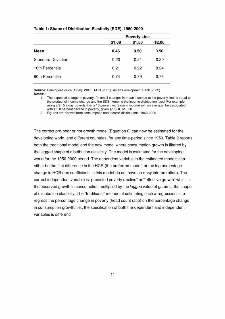
Table 1 reports on the estimated “shape of distribution” coefficients for three different

poverty lines - $1.08, $ 1.50, and $ 2, all in PPP 1993 prices. They all show a consistent

pattern – the means are clustered around 0.5, and the 10th and 90th percentile are

around 0.25 and 0.75 respectively. This robustness leads to the following two

conclusions. First, that a given amount of consumption growth, ceteris paribus , and no

distribution change, will only lead to a change of about half that amount in the HCR.

Thus, the statement should not be that a 20 percent growth in consumption “only” led to

a decline of 10 percentage points in the HCR. If this happens, growth has certainly been

neutral if not pro poor; second, this result holds at an average level, is highly non-linear,

and judgments about whether particular growth episodes have been pro or anti poor

have to be filtered by knowledge of what the shape of the distribution function was for

that time-period.

6This is the important difference, and non-equivalence, between the income coefficient of the

traditionally estimated model and the new formulation. To reiterate, the model estimated byKakwani, Ravallion etc. simply has the growth term on the right hand side; the correctly specifiedmodel has the growth term multiplied by the highly non-linear coefficient gamma.

10



Table 1: Shape of Distribution Elasticity (SDE), 1960-2000

Poverty Line

$1.08 $1.50 $2.00

Mean 0.46 0.50 0.50

Standard Deviation 0.20 0.21 0.20

10th Percentile 0.21 0.22 0.24

90th Percentile 0.74 0.79 0.76

Source: Deininger-Squire (1996); WIDER-UN (2001); Asian Development Bank (2002)Notes:

1. The expected change in poverty, for small changes in mean incomes at the poverty line, is equal tothe product of income change and the SDE, keeping the income distribution fixed. For example,using a $1.5 a day poverty line, a 10 percent increase in income will, on average, be associatedwith a 5.0 percent decline in poverty, given an SDE of 0.50.

2. Figures are derived from consumption and income distributions, 1960-2000

The correct pro-poor or not growth model (Equation 6) can now be estimated for the

developing world, and different countries, for any time-period since 1950. Table 2 reports

both the traditional model and the new model where consumption growth is filtered by

the lagged shape of distribution elasticity. The model is estimated for the developing

world for the 1950-2000 period. The dependent variable in the estimated models can

either be the first difference in the HCR (the preferred model) or the log percentagechange in HCR (the coefficients in this model do not have an easy interpretation). The

correct independent variable is “predicted poverty decline” or “‘effective growth” which is

the observed growth in consumption multiplied by the lagged value of gamma, the shape

of distribution elasticity. The “traditional” method of estimating such a regression is to

regress the percentage change in poverty (head count ratio) on the percentage change

in consumption growth, i.e., the specification of both the dependent and independent

variables is different!

11



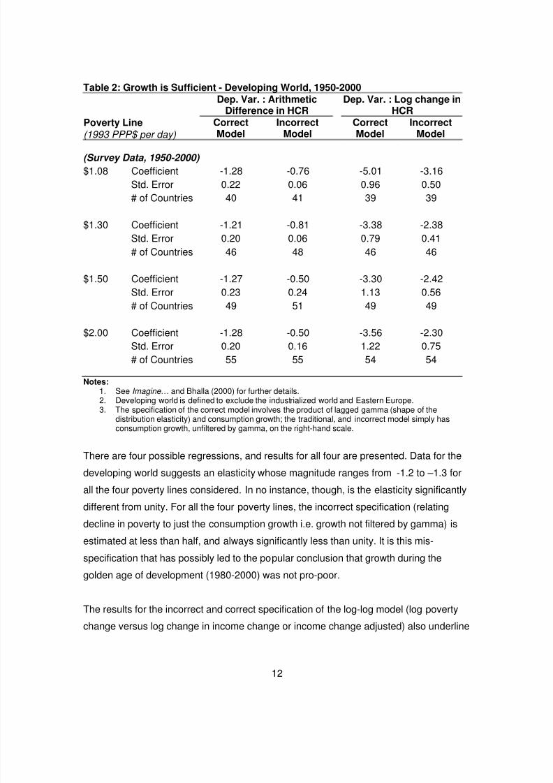
Table 2: Growth is Sufficient - Developing World, 1950-2000Dep. Var. : Arithmetic

Difference in HCRDep. Var. : Log change in

HCRPoverty Line

(1993 PPP$ per day)

Correct

Model

Incorrect

Model

Correct

Model

Incorrect

Model

(Survey Data, 1950-2000)

$1.08 Coefficient -1.28 -0.76 -5.01 -3.16

Std. Error 0.22 0.06 0.96 0.50

# of Countries 40 41 39 39

$1.30 Coefficient -1.21 -0.81 -3.38 -2.38

Std. Error 0.20 0.06 0.79 0.41


$1.50 Coefficient -1.27 -0.50 -3.30 -2.42

Std. Error 0.23 0.24 1.13 0.56


$2.00 Coefficient -1.28 -0.50 -3.56 -2.30

Std. Error 0.20 0.16 1.22 0.75


Notes:1. See Imagine … and Bhalla (2000) for further details.2. Developing world is defined to exclude the industrialized world and Eastern Europe.

3. The specification of the correct model involves the product of lagged gamma (shape of thedistribution elasticity) and consumption growth; the traditional, and incorrect model simply hasconsumption growth, unfiltered by gamma, on the right-hand scale.

There are four possible regressions, and results for all four are presented. Data for the

developing world suggests an elasticity whose magnitude ranges from -1.2 to –1.3 for

all the four poverty lines considered. In no instance, though, is the elasticity significantly

different from unity. For all the four poverty lines, the incorrect specification (relating

decline in poverty to just the consumption growth i.e. growth not filtered by gamma) is

estimated at less than half, and always significantly less than unity. It is this mis-

specification that has possibly led to the popular conclusion that growth during the

golden age of development (1980-2000) was not pro-poor.

The results for the incorrect and correct specification of the log-log model (log poverty

change versus log change in income change or income change adjusted) also underline

12



the importance of gamma. As modeled by others, the incorrect elasticity is observed to

be near 2 – actually around 2.3, with the lowest poverty line yielding this elasticity to be

3.2. In each instance, however, the correct specification yields to an elasticity that is

significantly higher, and higher by about 50 percent – centered around 3.4, and equal to

5 for the $1.08 poverty line.

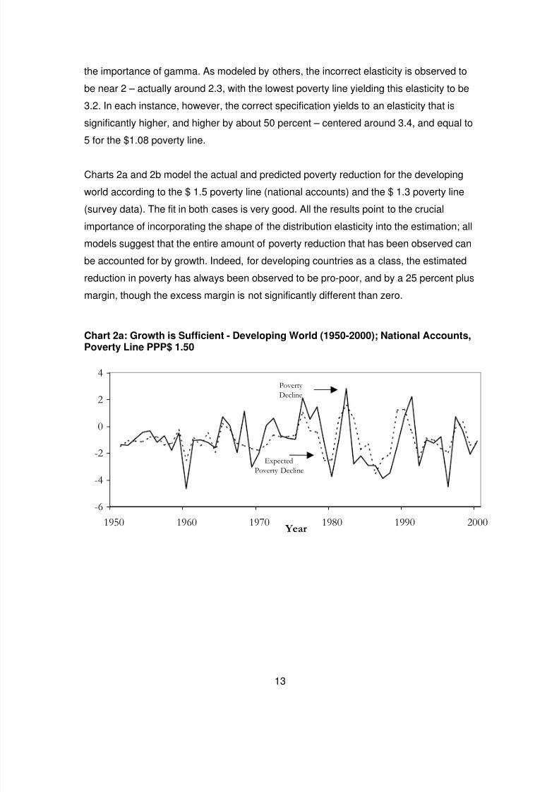
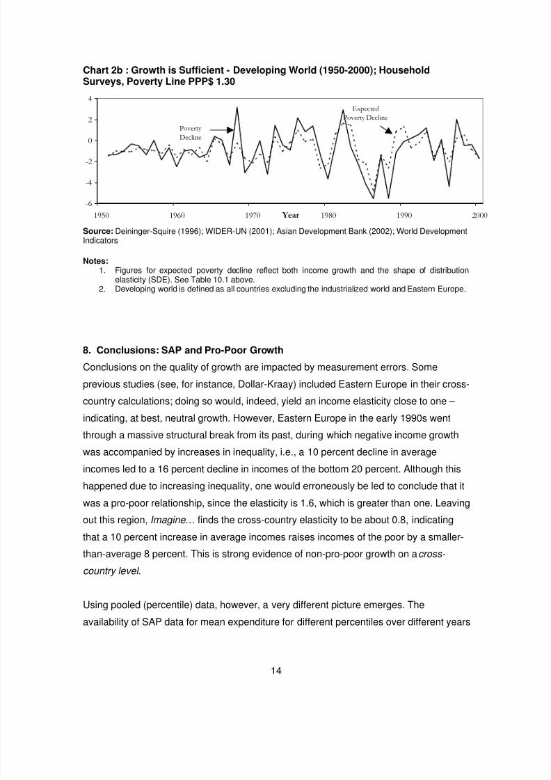
Charts 2a and 2b model the actual and predicted poverty reduction for the developing

world according to the $ 1.5 poverty line (national accounts) and the $ 1.3 poverty line

(survey data). The fit in both cases is very good. All the results point to the crucial

importance of incorporating the shape of the distribution elasticity into the estimation; all

models suggest that the entire amount of poverty reduction that has been observed can

be accounted for by growth. Indeed, for developing countries as a class, the estimated

reduction in poverty has always been observed to be pro-poor, and by a 25 percent plus

margin, though the excess margin is not significantly different than zero.

Chart 2a: Growth is Sufficient - Developing World (1950-2000); National Accounts,Poverty Line PPP$ 1.50

-6

-4

-2

0

2

4

1950 1960 1970 1980 1990 2000 Year

Poverty

Decline

Expected

Poverty Decline

13



Chart 2b : Growth is Sufficient - Developing World (1950-2000); HouseholdSurveys, Poverty Line PPP$ 1.30

-6

-4

-2

0

2

4

1950 1960 1970 1980 1990 2000 Year

Poverty

Decline

Expected

Poverty Decline

Source: Deininger-Squire (1996); WIDER-UN (2001); Asian Development Bank (2002); World DevelopmentIndicators

Notes:

1. Figures for expected poverty decline reflect both income growth and the shape of distributionelasticity (SDE). See Table 10.1 above.2. Developing world is defined as all countries excluding the industrialized world and Eastern Europe.

8. Conclusions: SAP and Pro-Poor Growth

Conclusions on the quality of growth are impacted by measurement errors. Some

previous studies (see, for instance, Dollar-Kraay) included Eastern Europe in their cross-

country calculations; doing so would, indeed, yield an income elasticity close to one –

indicating, at best, neutral growth. However, Eastern Europe in the early 1990s went

through a massive structural break from its past, during which negative income growth

was accompanied by increases in inequality, i.e., a 10 percent decline in average

incomes led to a 16 percent decline in incomes of the bottom 20 percent. Although this

happened due to increasing inequality, one would erroneously be led to conclude that it

was a pro-poor relationship, since the elasticity is 1.6, which is greater than one. Leaving

out this region, Imagine … finds the cross-country elasticity to be about 0.8, indicating

that a 10 percent increase in average incomes raises incomes of the poor by a smaller-

than-average 8 percent. This is strong evidence of non-pro-poor growth on a cross-

country level .

Using pooled (percentile) data, however, a very different picture emerges. The

availability of SAP data for mean expenditure for different percentiles over different years

14



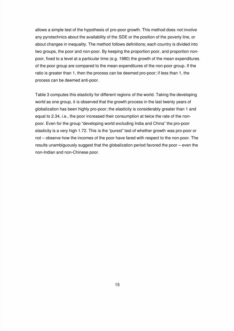
allows a simple test of the hypothesis of pro-poor growth. This method does not involve

any pyrotechnics about the availability of the SDE or the position of the poverty line, or

about changes in inequality. The method follows definitions; each country is divided into

two groups, the poor and non-poor. By keeping the proportion poor, and proportion non-

poor, fixed to a level at a particular time (e.g. 1980) the growth of the mean expenditures

of the poor group are compared to the mean expenditures of the non-poor group. If the

ratio is greater than 1, then the process can be deemed pro-poor; if less than 1, the

process can be deemed anti-poor.

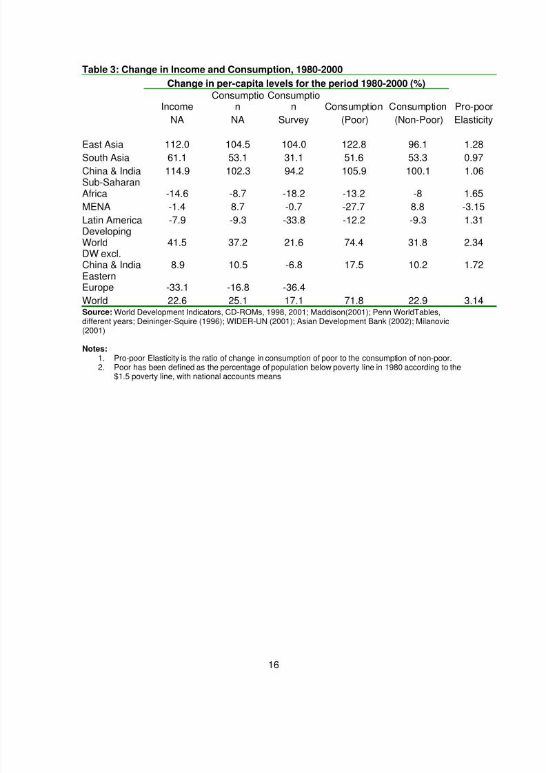
Table 3 computes this elasticity for different regions of the world. Taking the developing

world as one group, it is observed that the growth process in the last twenty years of

globalization has been highly pro-poor; the elasticity is considerably greater than 1 and

equal to 2.34, i.e., the poor increased their consumption at twice the rate of the non-

poor. Even for the group “developing world excluding India and China” the pro-poor

elasticity is a very high 1.72. This is the “purest” test of whether growth was pro-poor or

not – observe how the incomes of the poor have fared with respect to the non-poor. The

results unambiguously suggest that the globalization period favored the poor – even the

non-Indian and non-Chinese poor.

15



Table 3: Change in Income and Consumption, 1980-2000

Change in per-capita levels for the period 1980-2000 (%)

IncomeConsumptio

nConsumptio

n Consumption Consumption Pro-poor

NA NA Survey (Poor) (Non-Poor) Elasticity

East Asia 112.0 104.5 104.0 122.8 96.1 1.28

South Asia 61.1 53.1 31.1 51.6 53.3 0.97

China & India 114.9 102.3 94.2 105.9 100.1 1.06Sub-SaharanAfrica -14.6 -8.7 -18.2 -13.2 -8 1.65

MENA -1.4 8.7 -0.7 -27.7 8.8 -3.15

Latin America -7.9 -9.3 -33.8 -12.2 -9.3 1.31DevelopingWorld 41.5 37.2 21.6 74.4 31.8 2.34DW excl.China & India 8.9 10.5 -6.8 17.5 10.2 1.72EasternEurope -33.1 -16.8 -36.4

World 22.6 25.1 17.1 71.8 22.9 3.14Source: World Development Indicators, CD-ROMs, 1998, 2001; Maddison(2001); Penn WorldTables,different years; Deininger-Squire (1996); WIDER-UN (2001); Asian Development Bank (2002); Milanovic(2001)

Notes:1. Pro-poor Elasticity is the ratio of change in consumption of poor to the consumption of non-poor.2. Poor has been defined as the percentage of population below poverty line in 1980 according to the

$1.5 poverty line, with national accounts means

16



Policy Brief: Who has Lost out to Globalization?

Abstracted from Imagine There’s No Country: Poverty, Inequality and Growth in the era of Globalization , by Surjit S. Bhalla. Published by the Institute for International Economics, September 2002

1. Introduction & OverviewDespite globalization’s many benefits, indeed, despite it favoring the developing world by

its very nature, there is strong (and vocal) opposition to the process from certain groups.

This raises some important questions. What lies at the root of such opposition – reality,

or perception? Does globalization favor some groups (or countries) at the cost of others?

Evidence suggests that no one has “lost out” to globalization in an absolute sense.

There is, however, strong evidence of convergence during the last twenty-odd years.

There is consistent and strong evidence about how globalization is helping to equalize

wages for similar productivity levels, and the major beneficiaries here are the residents

of the developing world, particularly the two-thirds of the developing world that resides in

Asia. There is even stronger evidence that world inequality is in a declining mode for the

first time in 200 years. The strongest evidence pertains to the importance of the

globalization period for the poor countries, and the poor within these countries. Several

indicators of well-being (education, health, political and civil liberties) point to the fact

that the golden age of development has just been experienced.

Imagine …presents a strong case that the very success of globalization threatens a

single distinct group – the middle classes in the industrialized world – and thereby

generates the type (and the composition ) of opposition to globalization that has been

witnessed in the recent past. Very roughly, the world can be divided into two halves: the

developing countries, and the industrialized world. Within these halves are three broad

income groups: the poor (bottom 30 percent), the middle classes (the 30th to the 80th

percentile), and the rich (top 20 percent). It is useful to see how globalization has

impacted these groups. Significantly, the developing world in general (and the Asian

“elite”, or top 10 percent of the population, in particular) has achieved huge gains over

the past twenty years both in absolute terms, and especially relative to the industrialized

17



world’s middle classes. As a group, the developing world has achieved a 1 percentage

point per annum acceleration in growth rates during the globalization era (i.e., 3.1

percent growth per annum during 1980-2000, compared with 2.1 percent annually during

the previous twenty years). In stark contrast, the industrialized world has seen a

deceleration amounting to 1.7 percentage points per annum (1.6 percent per annum

growth now, 3.3 percent per annum in the previous twenty years). This, more than any

other factor, is responsible for the negative image that “globalization“ evokes in some.

The non-Asian third of the developing world was not very globalization-lucky. The

globalization period was not good for either Latin America or Africa, but the process of

globalization itself cannot be held responsible for this. (If anything, it may have been a

failure to participate fully in globalization that caused Latin America and Africa to

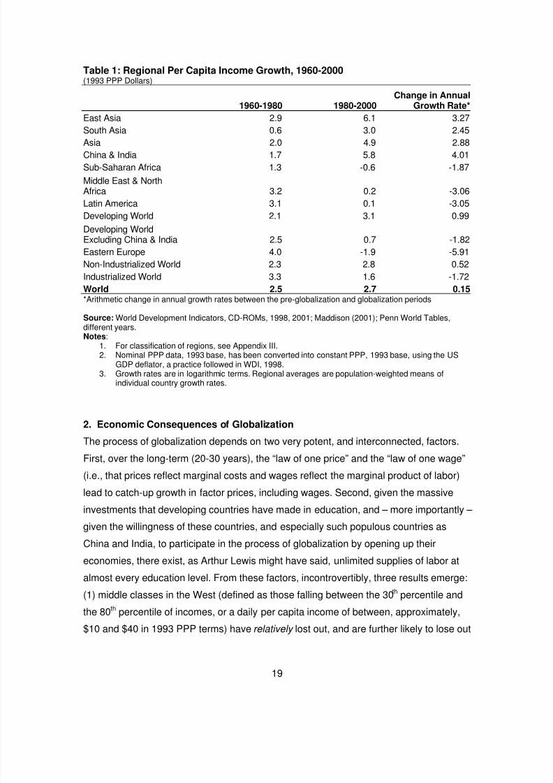
experience stagnation.) After almost doubling per-capita income from 1960 to 1980,

Latin American economies barely maintained their 1980 levels, and that too over a

twenty year period (Table 1). The genuinely tragic story is that of Sub-Saharan Africa,

which did worse as per capita incomes declined by 12 percent during the last two

decades. (It is little realized, but this region had more than double the per capita income

of Asia in 1960; today, the average Asian has double the income of an average African.)

The reasons for this stagnation are many, including, prominently, the devastation

wreaked by HIV/AIDS. For the world community, this should be the major target of

attention. On a positive note, there is no reason why the positive forces of globalization

should also not catch up with Africa.

18



Table 1: Regional Per Capita Income Growth, 1960-2000(1993 PPP Dollars)

1960-1980 1980-2000Change in Annual

Growth Rate*

East Asia 2.9 6.1 3.27

South Asia 0.6 3.0 2.45

Asia 2.0 4.9 2.88

China & India 1.7 5.8 4.01

Sub-Saharan Africa 1.3 -0.6 -1.87

Middle East & NorthAfrica 3.2 0.2 -3.06

Latin America 3.1 0.1 -3.05

Developing World 2.1 3.1 0.99

Developing WorldExcluding China & India 2.5 0.7 -1.82

Eastern Europe 4.0 -1.9 -5.91

Non-Industrialized World 2.3 2.8 0.52

Industrialized World 3.3 1.6 -1.72World 2.5 2.7 0.15*Arithmetic change in annual growth rates between the pre-globalization and globalization periods

Source: World Development Indicators, CD-ROMs, 1998, 2001; Maddison (2001); Penn World Tables,different years.Notes:

1. For classification of regions, see Appendix III.2. Nominal PPP data, 1993 base, has been converted into constant PPP, 1993 base, using the US

GDP deflator, a practice followed in WDI, 1998.3. Growth rates are in logarithmic terms. Regional averages are population-weighted means of

individual country growth rates.

2. Economic Consequences of Globalization

The process of globalization depends on two very potent, and interconnected, factors.

First, over the long-term (20-30 years), the “law of one price” and the “law of one wage”

(i.e., that prices reflect marginal costs and wages reflect the marginal product of labor)

lead to catch-up growth in factor prices, including wages. Second, given the massive

investments that developing countries have made in education, and – more importantly –

given the willingness of these countries, and especially such populous countries as

China and India, to participate in the process of globalization by opening up theireconomies, there exist, as Arthur Lewis might have said, unlimited supplies of labor at

almost every education level. From these factors, incontrovertibly, three results emerge:

(1) middle classes in the West (defined as those falling between the 30th percentile and

the 80th percentile of incomes, or a daily per capita income of between, approximately,

$10 and $40 in 1993 PPP terms) have relatively lost out, and are further likely to lose out

19



the most to the elite classes in the developing world; (2) world inequality has improved

significantly, and will continue to do so; and (3) the poor are also benefiting from

globalization. The first result, in particular, explains much of the opposition to

globalization.

3. Divergence or Convergence?

Did worldwide individual and country inequality worsen during the period of

globalization? The contention of Pritchett, UN, IMF and the World Bank (and others not

quoted) was that there was divergence in per capita output; while the simple data on per

capita output in developing and developed countries indicated just the opposite, and did

so in a convincing fashion. Are the divergent results a function of the time-period

chosen? No. Note that if one goes sufficiently back, especially to pre-Industrial

Revolution times, one will tautologically define and find divergence. Today, countries are

rich and poor; back then, all countries were the same.

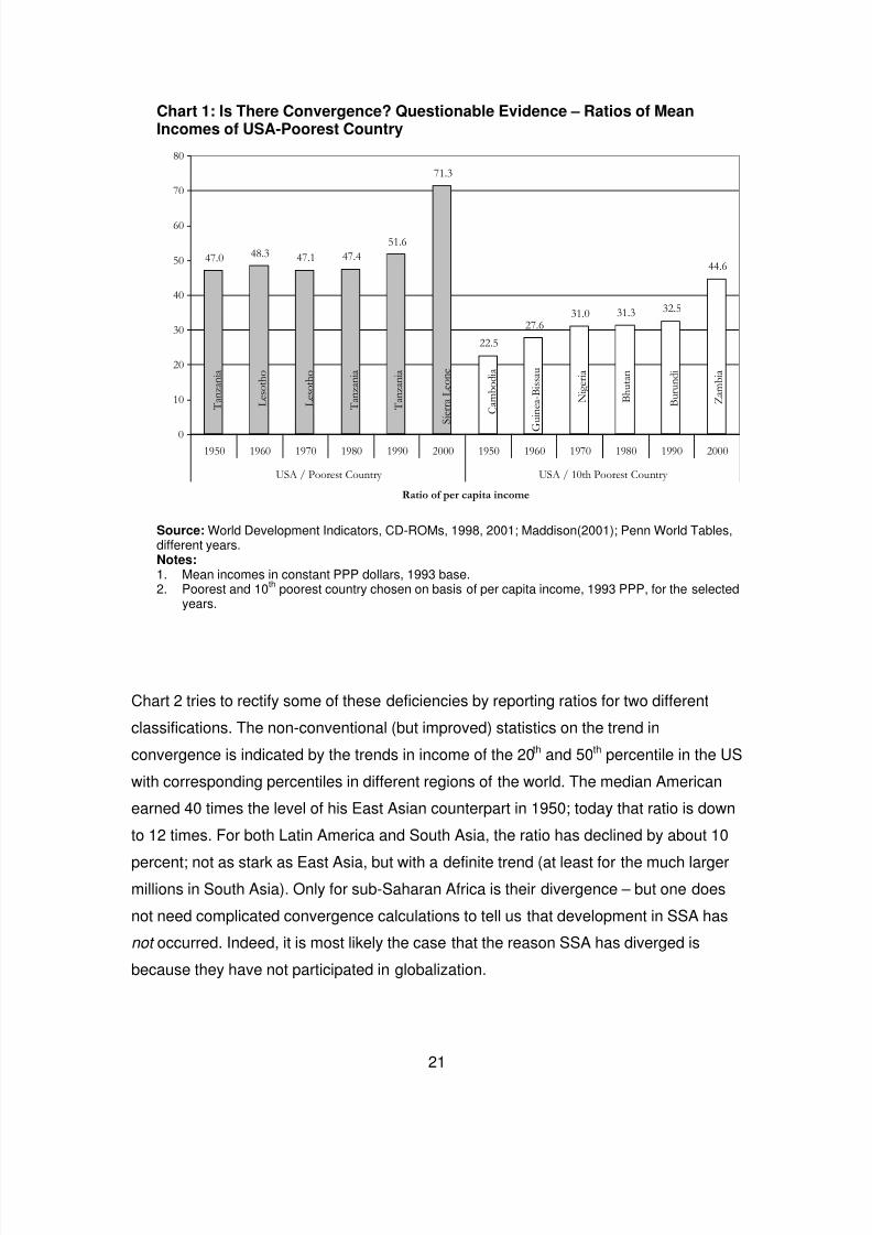
The real source of the difference between the distinguished divergence tribe and those

that argue that there has been overwhelming convergence is not in terms of the time-

period but in the set of statistics chosen. In particular, the divergent calculation is often

done in terms of the relative incomes of those residing at the technology frontier (the

richest country, typically the US) and those residing in the poorest country (one that is

changing continuously over time); this ratio suffers from a severe self-selection bias.

(Chart 1 illustrates the type of “evidence” that is often used to support the case for

divergence.) The second and equally severe problem with this self-selection analysis is

that its unit of analysis is the poorest country rather than the poorest people . And even if

it were the poorest people, it should be the poorest fraction of people.

20



Chart 1: Is There Convergence? Questionable Evidence – Ratios of MeanIncomes of USA-Poorest Country

47.0 48.3 47.1 47.4

51.6

71.3

22.5

27.631.0 31.3 32.5

44.6

0

10

20

30

40

50

60

70

80

1950 1960 1970 1980 1990 2000 1950 1960 1970 1980 1990 2000

USA / Poorest Country USA / 10th Poorest Country

Ratio of per capita income

T a n z a n i a

L e s o t h o

L e s o t h o

T a n z a n i a

T a n z a n i a

S i e r r a L e o n e

C a m b o d i a

G u i n e a - B i s s a u

N i g e r i a

B h u t a n

B u r u n d i

Z a m b i a

Source: World Development Indicators, CD-ROMs, 1998, 2001; Maddison(2001); Penn World Tables,different years.Notes:1. Mean incomes in constant PPP dollars, 1993 base.2. Poorest and 10

thpoorest country chosen on basis of per capita income, 1993 PPP, for the selected

years.

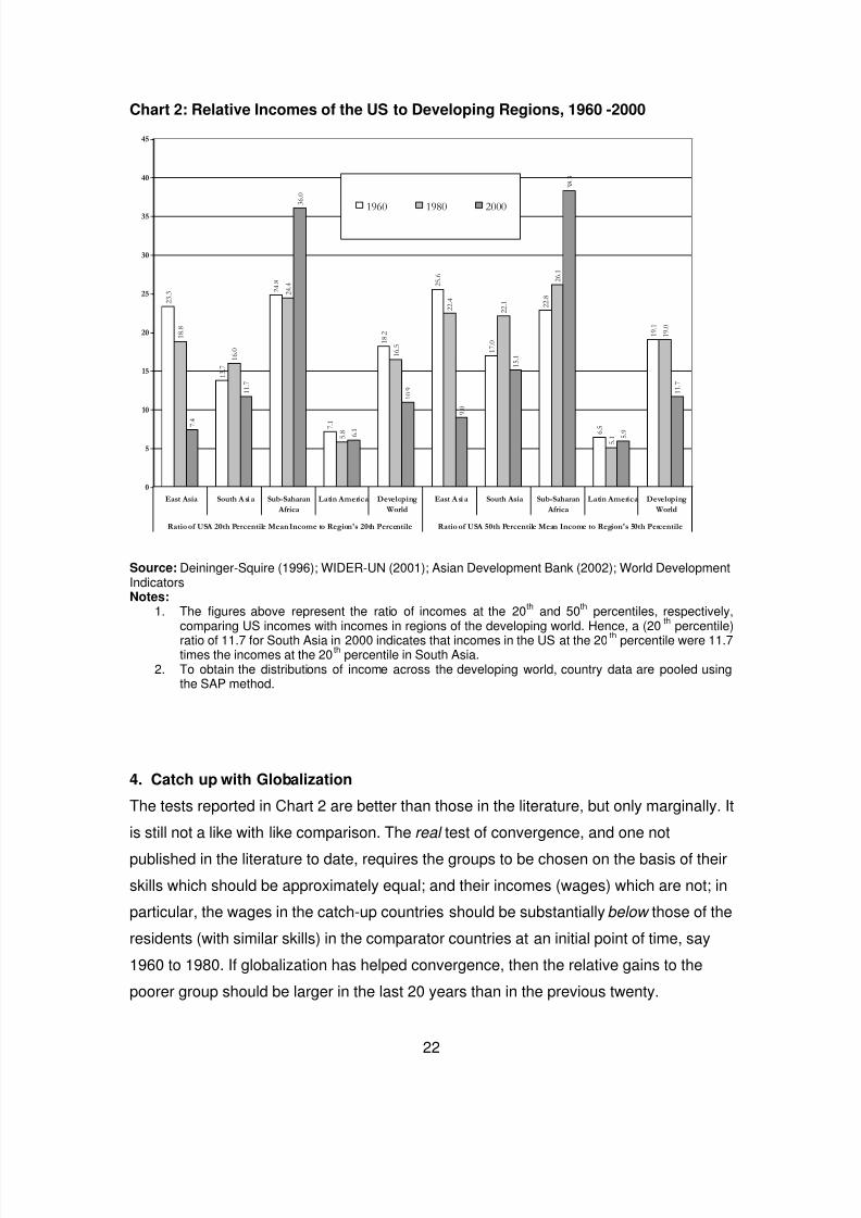
Chart 2 tries to rectify some of these deficiencies by reporting ratios for two different

classifications. The non-conventional (but improved) statistics on the trend in

convergence is indicated by the trends in income of the 20th and 50th percentile in the US

with corresponding percentiles in different regions of the world. The median American

earned 40 times the level of his East Asian counterpart in 1950; today that ratio is down

to 12 times. For both Latin America and South Asia, the ratio has declined by about 10

percent; not as stark as East Asia, but with a definite trend (at least for the much largermillions in South Asia). Only for sub-Saharan Africa is their divergence – but one does

not need complicated convergence calculations to tell us that development in SSA has

not occurred. Indeed, it is most likely the case that the reason SSA has diverged is

because they have not participated in globalization.

21



Chart 2: Relative Incomes of the US to Developing Regions, 1960 -2000

2 3 . 3

1 3 . 7

2 4 . 8

7 . 1

1 8 . 2

2 5 . 6

1 7 . 0

2 2 . 8

6 . 5

1 9 . 1

1 8 . 8

1 6 . 0

2 4 . 4

5 . 8

1 6 . 5

2 2 . 4

2 2 . 1

2 6 . 1

5 . 1

1 9 . 0

7

. 4

1 1 . 7

3 6 . 0

6 . 1

1 0 . 9

9 . 0

1 5 . 1

3 8 . 3

5 . 9

1 1 . 7

0

5

10

15

20

25

30

35

40

45

East Asia South A si a Sub-Saharan

Africa

Latin America Developing

World

East A si a South Asia Sub-Saharan

Africa

Latin America Developing

World

Ratio of USA 20th Percentile Mean Income to Region's 20th Percentile Ratio of USA 50th Percentile Mean Income to Region's 50th Percentile

1960 1980 2000

Source: Deininger-Squire (1996); WIDER-UN (2001); Asian Development Bank (2002); World DevelopmentIndicatorsNotes:

1. The figures above represent the ratio of incomes at the 20th

and 50th

percentiles, respectively,comparing US incomes with incomes in regions of the developing world. Hence, a (20

thpercentile)

ratio of 11.7 for South Asia in 2000 indicates that incomes in the US at the 20th

percentile were 11.7times the incomes at the 20

thpercentile in South Asia.

2. To obtain the distributions of income across the developing world, country data are pooled usingthe SAP method.

4. Catch up with Globalization

The tests reported in Chart 2 are better than those in the literature, but only marginally. It

is still not a like with like comparison. The real test of convergence, and one not

published in the literature to date, requires the groups to be chosen on the basis of their

skills which should be approximately equal; and their incomes (wages) which are not; in

particular, the wages in the catch-up countries should be substantially below those of the

residents (with similar skills) in the comparator countries at an initial point of time, say

1960 to 1980. If globalization has helped convergence, then the relative gains to the

poorer group should be larger in the last 20 years than in the previous twenty.

22



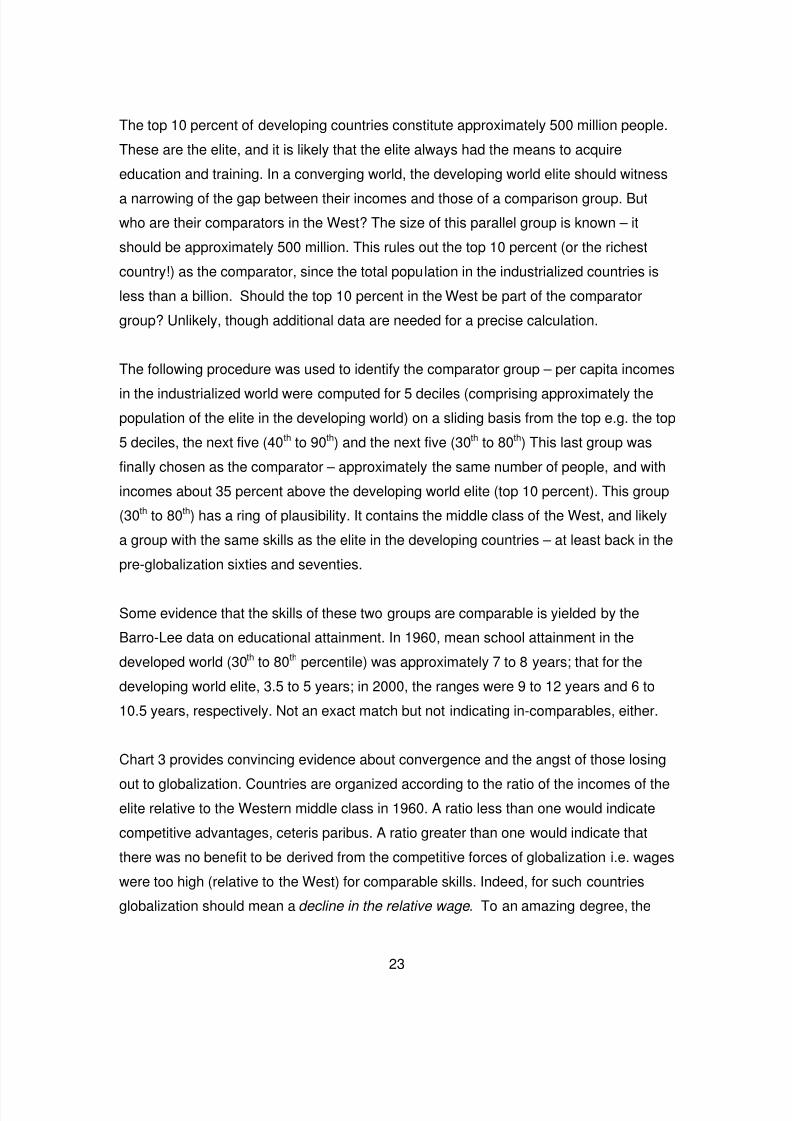
The top 10 percent of developing countries constitute approximately 500 million people.

These are the elite, and it is likely that the elite always had the means to acquire

education and training. In a converging world, the developing world elite should witness

a narrowing of the gap between their incomes and those of a comparison group. But

who are their comparators in the West? The size of this parallel group is known – it

should be approximately 500 million. This rules out the top 10 percent (or the richest

country!) as the comparator, since the total population in the industrialized countries is

less than a billion. Should the top 10 percent in the West be part of the comparator

group? Unlikely, though additional data are needed for a precise calculation.

The following procedure was used to identify the comparator group – per capita incomes

in the industrialized world were computed for 5 deciles (comprising approximately the

population of the elite in the developing world) on a sliding basis from the top e.g. the top

5 deciles, the next five (40 th to 90th) and the next five (30th to 80th) This last group was

finally chosen as the comparator – approximately the same number of people, and with

incomes about 35 percent above the developing world elite (top 10 percent). This group

(30th to 80th) has a ring of plausibility. It contains the middle class of the West, and likely

a group with the same skills as the elite in the developing countries – at least back in the

pre-globalization sixties and seventies.

Some evidence that the skills of these two groups are comparable is yielded by the

Barro-Lee data on educational attainment. In 1960, mean school attainment in the

developed world (30th to 80th percentile) was approximately 7 to 8 years; that for the

developing world elite, 3.5 to 5 years; in 2000, the ranges were 9 to 12 years and 6 to

10.5 years, respectively. Not an exact match but not indicating in-comparables, either.

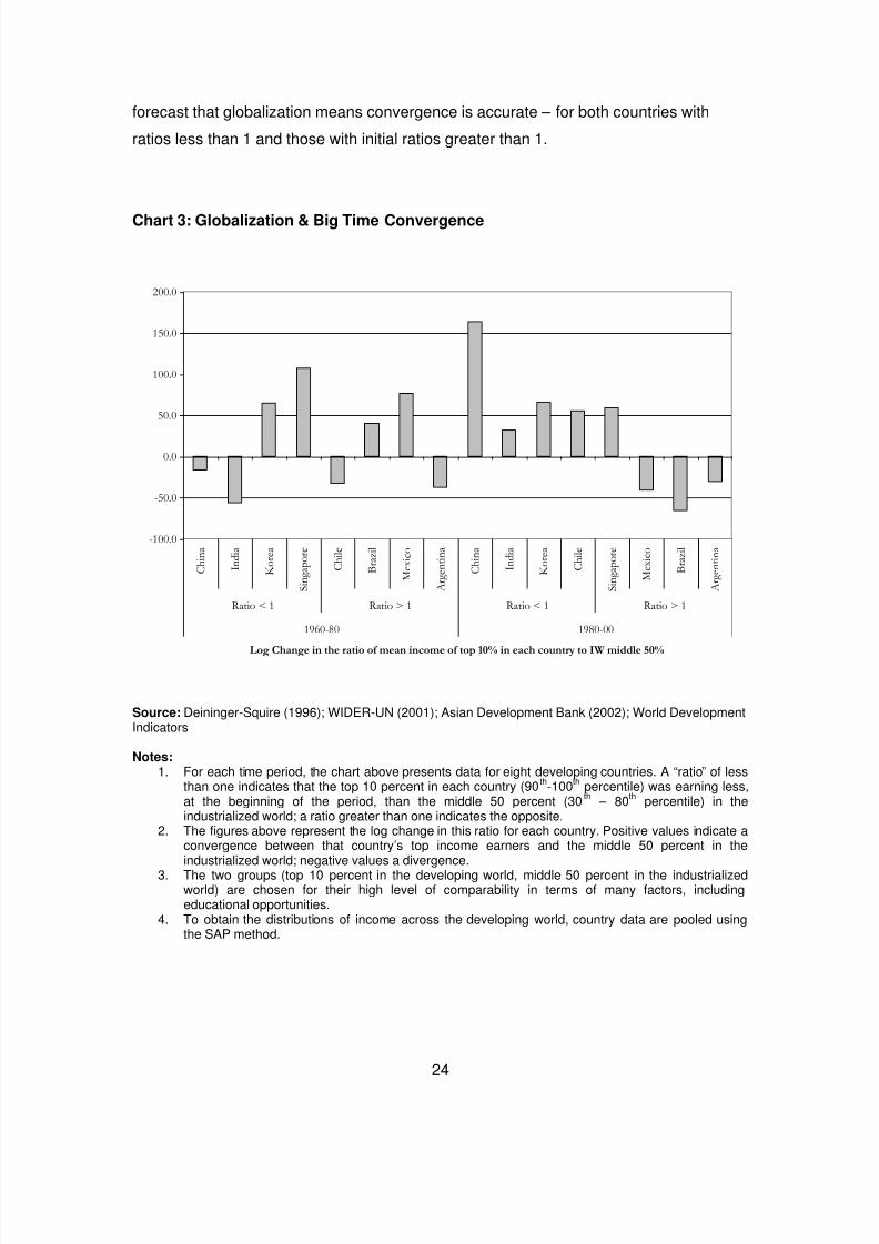
Chart 3 provides convincing evidence about convergence and the angst of those losing

out to globalization. Countries are organized according to the ratio of the incomes of theelite relative to the Western middle class in 1960. A ratio less than one would indicate

competitive advantages, ceteris paribus. A ratio greater than one would indicate that

there was no benefit to be derived from the competitive forces of globalization i.e. wages

were too high (relative to the West) for comparable skills. Indeed, for such countries

globalization should mean a decline in the relative wage . To an amazing degree, the

23



forecast that globalization means convergence is accurate – for both countries with

ratios less than 1 and those with initial ratios greater than 1.

Chart 3: Globalization & Big Time Convergence

-100.0

-50.0

0.0

50.0

100.0

150.0

200.0

C h i n a

I n d i a

K o r e a

S i n g a p o r e

C h i l e

B r a z i l

M e x i c o

A r g e n t i n a

C h i n a

I n d i a

K o r e a

C h i l e

S i n g a p o r e

M e x i c o

B r a z i l

A r g e n t i n a

Ratio < 1 Ratio > 1 Ratio < 1 Ratio > 1

1960-80 1980-00

Log Change in the ratio of mean income of top 10% in each country to IW middle 50%

Source: Deininger-Squire (1996); WIDER-UN (2001); Asian Development Bank (2002); World DevelopmentIndicators

Notes:1. For each time period, the chart above presents data for eight developing countries. A “ratio” of less

than one indicates that the top 10 percent in each country (90th

-100th

percentile) was earning less,at the beginning of the period, than the middle 50 percent (30

th– 80

thpercentile) in the

industrialized world; a ratio greater than one indicates the opposite.2. The figures above represent the log change in this ratio for each country. Positive values indicate a

convergence between that country’s top income earners and the middle 50 percent in theindustrialized world; negative values a divergence.

3. The two groups (top 10 percent in the developing world, middle 50 percent in the industrializedworld) are chosen for their high level of comparability in terms of many factors, includingeducational opportunities.

4. To obtain the distributions of income across the developing world, country data are pooled usingthe SAP method.

24



From 1960 to 1980, the elite in Asian countries had income (wages) relative to their

comparators of approximately 41 percent i.e. the middle class westerners had incomes

approximately two and a half times that of the Asian elite. During this golden age of the

western middle class, real incomes almost doubled registering an annual growth of 3.2

percent per year. Aspirations are built on experience, and the experience was very good.

The Asian elite (constituting about three-fourths of the developing world elite per se ) also

matched the progress of their Western counterparts; their relative income had inched up

to 43 percent, from 40 percent earlier. The next twenty years turned out to be the golden

age for Asia. While the growth in the absolute incomes of the Western middle class

slowed down to a crawl – only 1.3 percent per annum, less than half of that experienced

by their parents – that of the Asian elite accelerated – to 4.7 percent per annum,

compared with 3 percent in the 1960-80 period, or a 93 percent period increase,

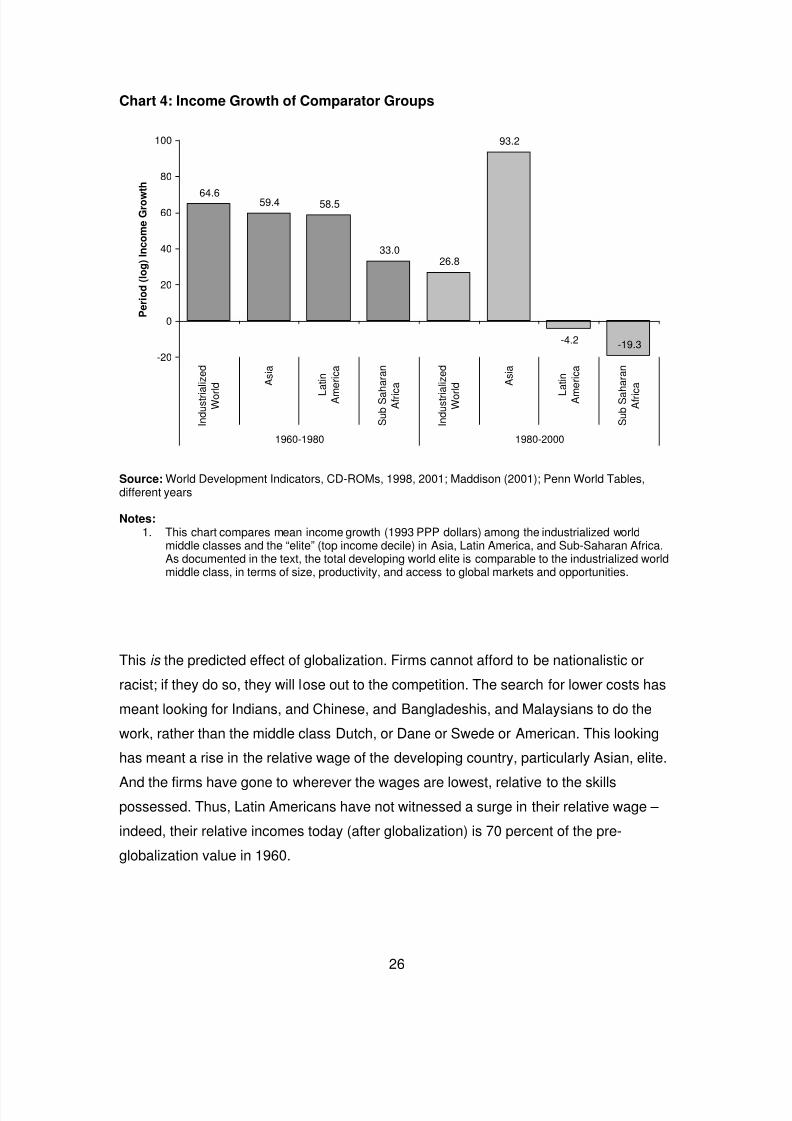
compared with 59 percent in the previous twenty years (Chart 4). The relative incomes

of the Asian elite (the one of concern for tests of convergence) accelerated to 60 percent

of their counterpart incomes in 2000. This relative income, as mentioned above, was 43

percent in 1980.

25



Chart 4: Income Growth of Comparator Groups

64.6 59.4 58.5

33.026.8

93.2

-4.2 -19.3-20

0

20

40

60

80

100

I n d u s t r i a l i z e d

W o r l d A

s i a

L

a t i n

A m

e r i c a

S u b S a h a r a n

A f r i c

a

I n d u s t r i a l i z e d

W o r l d A

s i a

L

a t i n

A m

e r i c a

S u b S a h a r a n

A f r i c

a

1960-1980 1980-2000

P e r i o d ( l o g ) I n c o m e G r o w

t h

Source: World Development Indicators, CD-ROMs, 1998, 2001; Maddison (2001); Penn World Tables,different years

Notes:1. This chart compares mean income growth (1993 PPP dollars) among the industrialized world

middle classes and the “elite” (top income decile) in Asia, Latin America, and Sub-Saharan Africa.As documented in the text, the total developing world elite is comparable to the industrialized worldmiddle class, in terms of size, productivity, and access to global markets and opportunities.

This is the predicted effect of globalization. Firms cannot afford to be nationalistic or

racist; if they do so, they will lose out to the competition. The search for lower costs has

meant looking for Indians, and Chinese, and Bangladeshis, and Malaysians to do the

work, rather than the middle class Dutch, or Dane or Swede or American. This looking

has meant a rise in the relative wage of the developing country, particularly Asian, elite.

And the firms have gone to wherever the wages are lowest, relative to the skillspossessed. Thus, Latin Americans have not witnessed a surge in their relative wage –

indeed, their relative incomes today (after globalization) is 70 percent of the pre-

globalization value in 1960.

26



5. Conclusions

There is an explanation for why there is a protest against globalization – only it does not

have anything to do with the poor getting poorer, or the rich getting richer faster. The

explanation is that because of globalization, the entire middle class in the North has had

to lower its expectations of a better life. It is the “poor elite” in the South that is getting

richer at a faster pace than that experienced by almost any such large group of people

(500 million) in history. The middle class in the North feels it is at their expense and they

are at least partially right.

Globalization is a democratic force; it is the ultimate leveler; and a force not kind to those

“unnaturally” at the top of the heap. It is a very visible process, abruptly changing

employment possibilities, challenging social norms etc. Structural adjustment- and

conditionality-linked credit from the World Bank or the IMF is linked in popular perception

with globalization; so, too, is privatization or the shutting down of often-inefficient state-

owned enterprises. Perception (clouded, as it often is, by ideology) says that such

externally-imposed changes must be bad for the nation, and especially bad for the poor;

cold, hard numbers say that, in fact, globalization is very good , both for the poor, and for

the middle classes and the elite in the developing world.

One should be witnessing Latin Americans as the leaders of the anti-globalization

brigade, but one does not. Perhaps they realize that in the uncompetitive world of the

sixties, they derived rents from their closeness to Western markets, and that with lower

transaction costs (almost zero in the age of the internet and instant communication)

these rents have disappeared. One should not be seeing Asians in the anti-globalization

camp, and one does not. One should be seeing middle-class Westerners disappointed

with what globalization has brought for them – more competition for their skills, a

decrease in their rents, and a sharp fall in their expectations for future growth. A collapse

from a 3.2 percent annual growth, or a doubling in real incomes in one generation, to an

increase of only 1.3 percent a year or a doubling in 55 years (three generations) andperhaps not even in one’s working life. To be sure, one does witness non-white

intellectuals articulating anti-globalization theses; why this is so is more a question for a

psychiatrist to answer, rather than an economist.

27



References

Asian Development Bank, (2001), RETA-5917, “Research Project on Developing aPoverty Database”,

Bhalla, Surjit, (2002), Imagine There’s no Country: Poverty, Inequality and Growth in the era of Globalization . Washington, D.C.: Institute for International Economics

Collier, Paul, and Dollar, David, (2000), “Can the World Cut Poverty in Half? How policyReform and Effective Aid can meet the International Development Goals”, mimeo,Development Research Group, World Bank, July.

Deininger, Klaus, and Lyn Squire, (1996), “A new data set measuring income inequality”,World Bank Economic Review, September.

Dollar, David, and Kraay, Aart, (2001), “Trade, Growth and Poverty”, mimeo, WorldBank, March.

Kakwani, Nanak, (1997), “On Measuring Growth and Inequality Components of Changesin Poverty with Application to Thailand”, forthcoming, Journal of Quantitative Economics.

Maddison, Angus, (2001), The World Economy: A Millennial Perspective , DevelopmentCenter of the Organisation for Economic Co-Operation and Development, April.

Prichett, Lant, (2001), “Divergence, Big Time”, mimeo, World Bank, July 7.

Ravallion, Martin, and Datt, Gaurav, (1999), “ When is Growth Pro-Poor?”, Evidencefrom the Diverse Experiences of India’s States”, mimeo, World Bank’s PovertyReduction and Economic Management Week, , Washington DC, July.

United Nations, Human Development Report 1999 , Oxford University Press.

WIDER – U.N, (2001), “World Income Inequality Database”, available atwww.wider.unu.edu/wiid.

World Bank, World Development Indicators, CD-ROMS, 1996-2001.

World Bank, (2000), World Development Report: Attacking Poverty , Oxford UniversityPress, Washington DC.

http://www.wider.unu.edu/wiid

http://www.wider.unu.edu/wiid

Documents

12978 Surjit Bhalla Two Policy Briefs