Entropy of mixing gas

Masatsugu Sei Suzuki

Department of Physics, SUNY at Binghamton

(Date: Septemnrt 09, 2017)

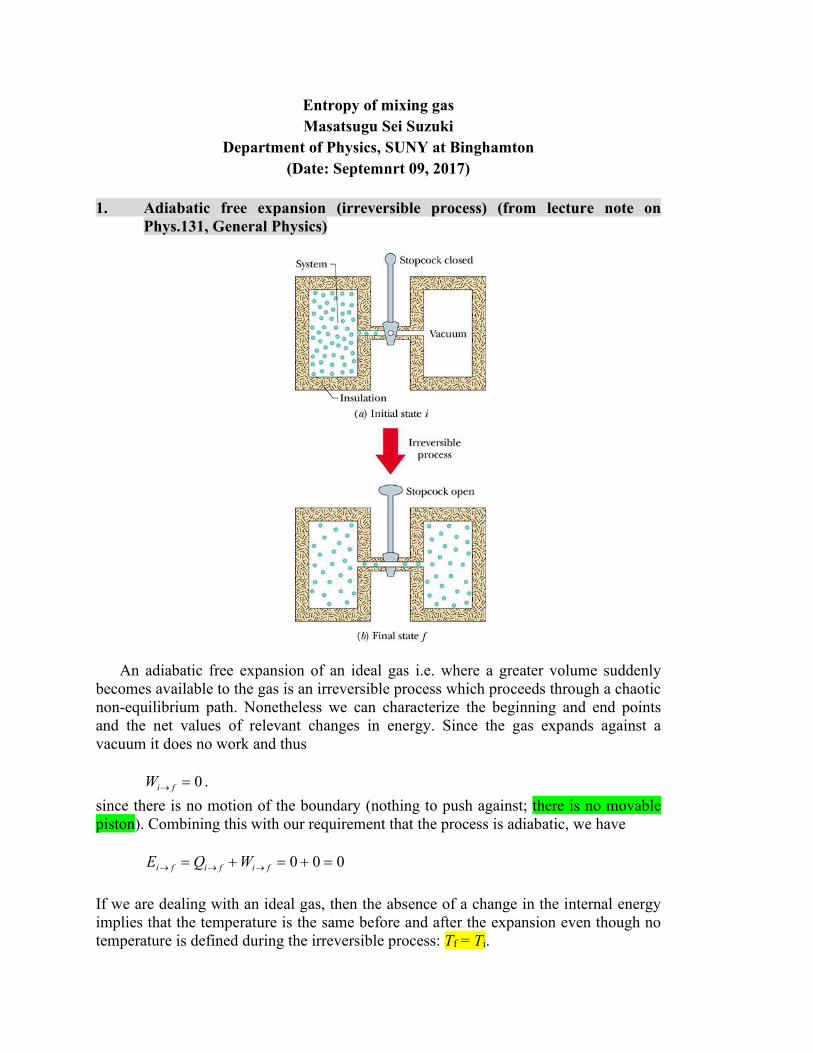
1. Adiabatic free expansion (irreversible process) (from lecture note on

Phys.131, General Physics)

An adiabatic free expansion of an ideal gas i.e. where a greater volume suddenly

becomes available to the gas is an irreversible process which proceeds through a chaotic

non-equilibrium path. Nonetheless we can characterize the beginning and end points

and the net values of relevant changes in energy. Since the gas expands against a

vacuum it does no work and thus

0 fiW .

since there is no motion of the boundary (nothing to push against; there is no movable

piston). Combining this with our requirement that the process is adiabatic, we have

000 fififi WQE

If we are dealing with an ideal gas, then the absence of a change in the internal energy

implies that the temperature is the same before and after the expansion even though no

temperature is defined during the irreversible process: Tf = Ti.

In order to calculate the entropy of this process, we need to find an equivalent

reversible path that shares the same initial and final state. A simple choice is an

isothermal, reversible expansion in which the gas pushes slowly against a piston. Using

the equation of state for an ideal gas this implies that

ffii VPVP

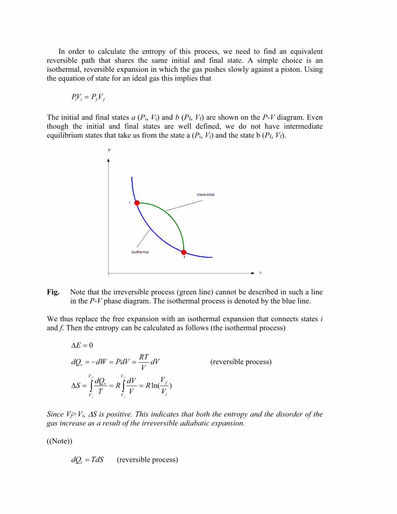
The initial and final states a (Pi, Vi) and b (Pf, Vf) are shown on the P-V diagram. Even

though the initial and final states are well defined, we do not have intermediate

equilibrium states that take us from the state a (Pi, Vi) and the state b (Pf, Vf).

Fig. Note that the irreversible process (green line) cannot be described in such a line

in the P-V phase diagram. The isothermal process is denoted by the blue line.

We thus replace the free expansion with an isothermal expansion that connects states i

and f. Then the entropy can be calculated as follows (the isothermal process)

)ln(

0

i

f

V

V

V

V

r

r

V

VR

V

dVR

T

dQS

dVV

RTPdVdWdQ

E

f

i

f

i

(reversible process)

Since Vf>Vi, S is positive. This indicates that both the entropy and the disorder of the

gas increase as a result of the irreversible adiabatic expansion.

((Note))

TdSdQr (reversible process)

dST

dQirr

Even if 0irrdQ (adiabatic process),

0dS .

Note that 0dS for the irreversible process and 0dS for the reversible process.

2. The entropy for the adiabatic free expansion (microscopic states)

Entropy can be treated from a microscopic viewpoint through statistical analysis of

molecular motions. We consider a microscopic model to examine the free expansion of

an ideal gas. The gas molecules are represented as particles moving randomly. Suppose

that the gas is initially confined to the volume Vi. When the membrane is removed, the

molecules eventually are distributed throughout the greater volume Vf of the entire

container. For a given uniform distribution of gas in the volume, there are a large

number of equivalent microstates, and the entropy of the gas can be related to the

number of microstates corresponding to a given macro-state.

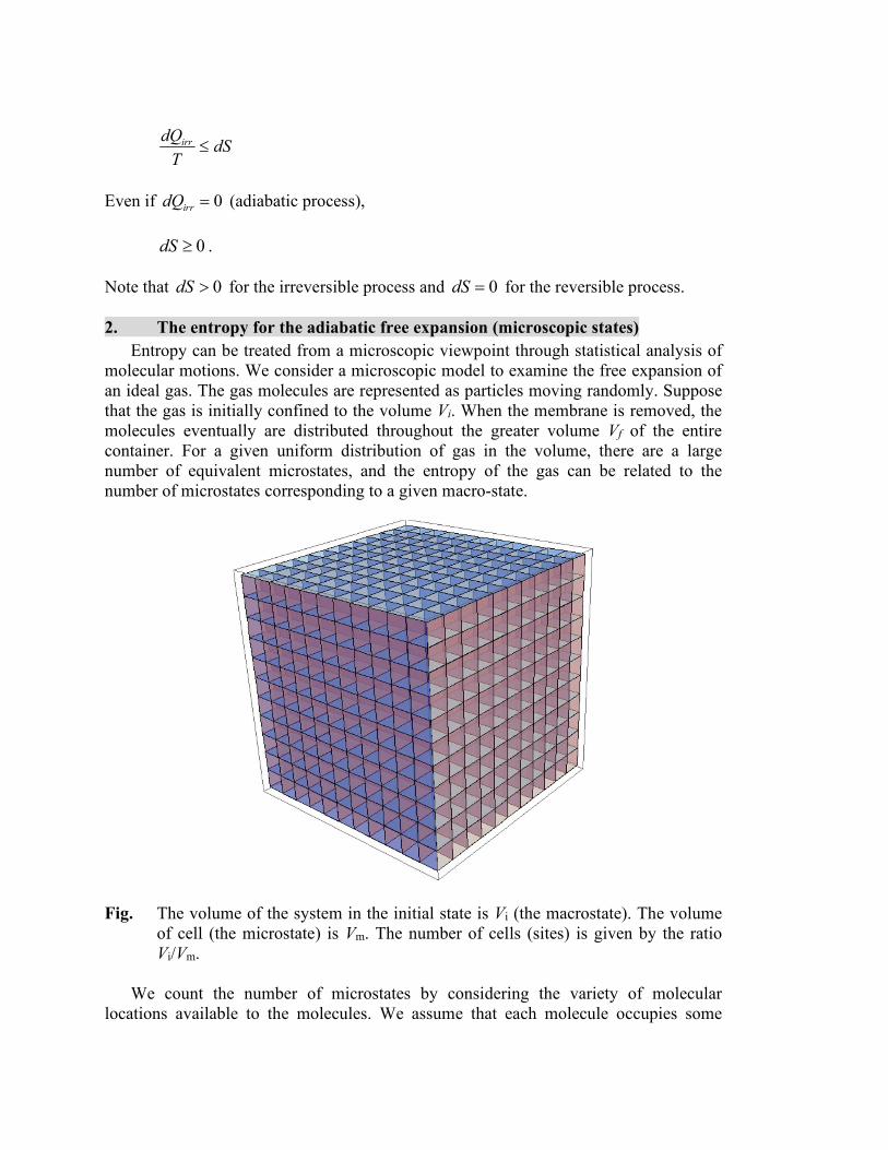
Fig. The volume of the system in the initial state is Vi (the macrostate). The volume

of cell (the microstate) is Vm. The number of cells (sites) is given by the ratio

Vi/Vm.

We count the number of microstates by considering the variety of molecular

locations available to the molecules. We assume that each molecule occupies some

microscopic volume mV . The total number of possible locations of a single molecule in

a macroscopic initial volume iV is the ratio

m

ii

V

Vw ,

which is a very large number. The number iw represents the number of the microstates,

or the number of available sites. We assume that the probability of a molecule

occupying any of these sites are equal.

Neglecting the very small probability of having two molecules occupy the same site,

each molecule may go into any of the wi sites, and so the number of ways of locating N

molecules in the volume becomes

N

m

iN

iiV

VwW

.

Similarly, when the volume is increased to Vf, the number of ways of locating N

molecules increases to

N

m

fN

ffV

VwW

.

Then the change of entropy is obtained as

)ln(

)]ln()[ln(

)]ln()[ln()]ln()[ln(

lnln

lnln

i

f

B

ifB

miBmfB

N

m

iB

N

m

f

B

iBfB

if

V

VNk

VVNk

VVNkVVNk

V

Vk

V

Vk

WkWk

SSS

When ANN , we have

)ln()ln(i

f

i

f

BAV

VR

V

VkNS

We note that the entropy S is related to the number of microstates for a given macrostate

as

WkS B ln .

The more microstates there are that correspond to a given macrostate, the greater the

entropy of that macrostate. There are many more microstates associated with disordered

macrostates than with ordered macrostates. Therefore, it is concluded that the entropy is

a measure of disorder. Although our discussion used the specific example of the

adiabatic free expansion of an ideal gas, a more rigorous development of the statistical

interpretation of entropy would lead us to the same conclusion.

3. Entropy change of mixing gas

((Kubo, Thermodynamics))

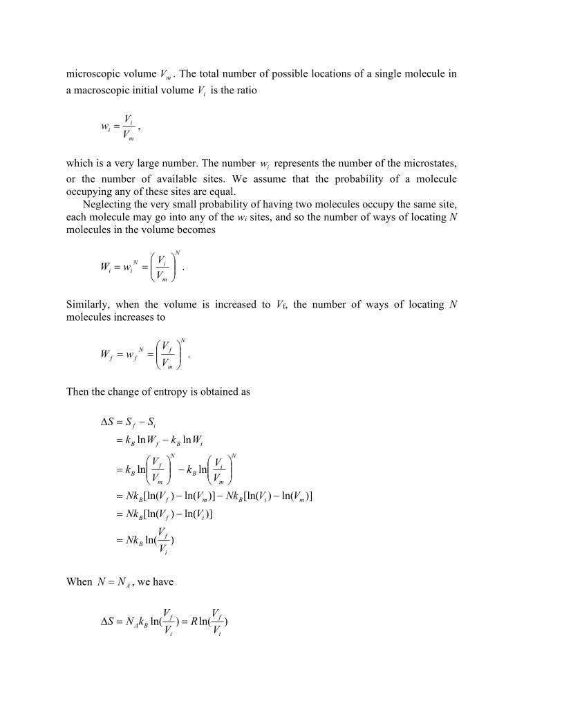
Two kinds of ideal gases at equal pressure and temperature, initially separated into

two containers, are mixed by diffusion. Show that the entropy is increased in this

process by an amount

)]ln()ln([21

22

21

11

nn

nn

nn

nnRS

where n1 and n2 are the moles of components gasses. Assume that no change in pressure

and temperature occurs due to the diffusion and the partial pressure of each gas in the

mixture is proportional to the molar concentration.

Fig. Initial state. Two gases are separated into two containers by a wall.

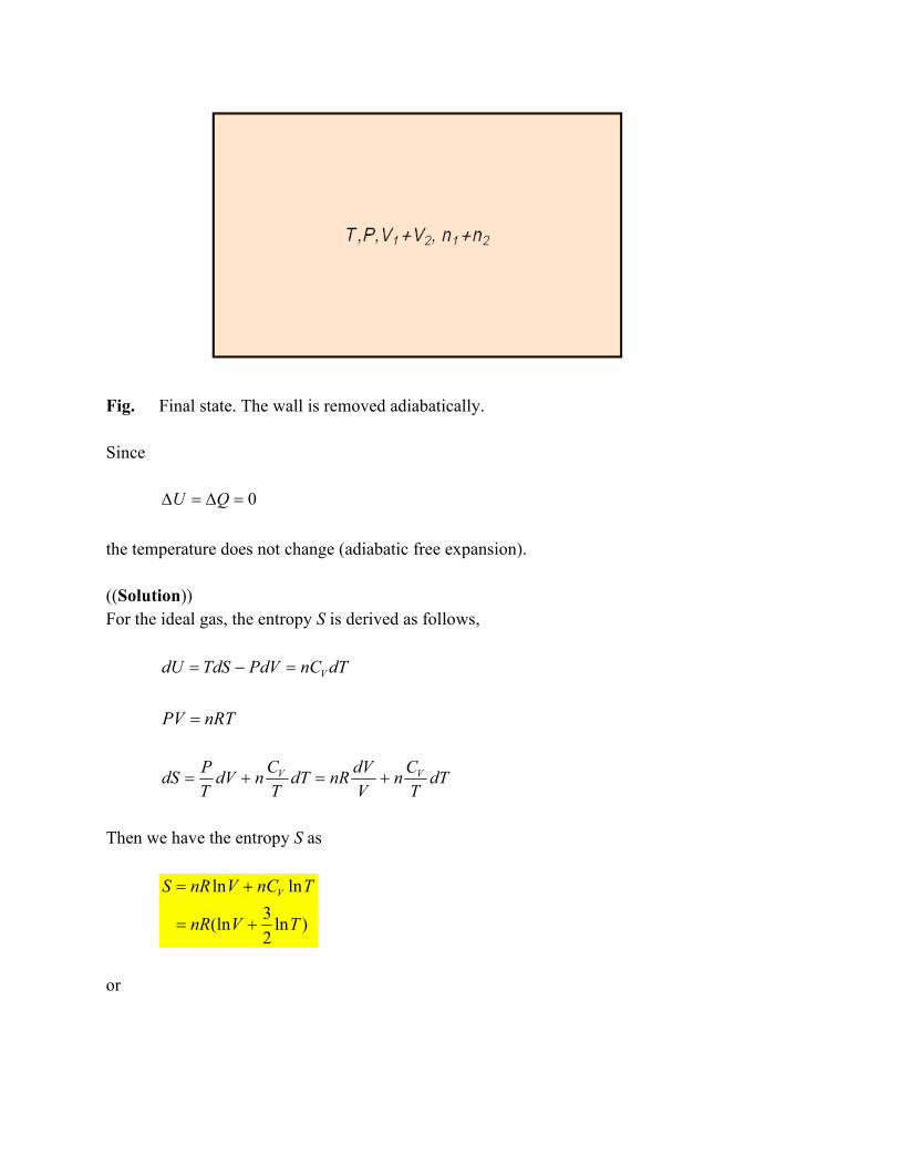
Fig. Final state. The wall is removed adiabatically.

Since

0 QU

the temperature does not change (adiabatic free expansion).

((Solution))

For the ideal gas, the entropy S is derived as follows,

dTnCPdVTdSdU V

nRTPV

dTT

Cn

V

dVnRdT

T

CndV

T

PdS VV

Then we have the entropy S as

)ln2

3(ln

lnln

TVnR

TnCVnRS V

or

)ln(]lnln[

)ln(lnln)(

)]ln(ln[lnln

)ln(ln

nRnCPCVCn

nRnCPnCVCRn

nRVPnCVnR

nR

PVnCVnRS

VVP

VVV

V

V

where we use RCV2

3 .

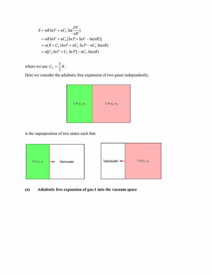
Here we consider the adiabatic free expansion of two gases independently.

is the superposition of two states such that

(a) Adiabatic free expansion of gas-1 into the vacuum space

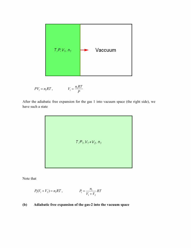
RTnPV 11 , P

RTnV 1

1

After the adiabatic free expansion for the gas 1 into vacuum space (the right side), we

have such a state

Note that

RTnVVP 1211 )( , RTVV

nP

21

11

(b) Adiabatic free expansion of the gas-2 into the vacuum space

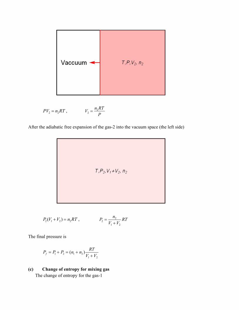
RTnPV 22 , P

RTnV 2

2

After the adiabatic free expansion of the gas-2 into the vacuum space (the left side)

RTnVVP 2212 )( , RTVV

nP

21

22

The final pressure is

21

2121 )(VV

RTnnPPPf

(c) Change of entropy for mixing gas

The change of entropy for the gas-1

1 1 1 2 1 1 1 1

1 21

1

[ ln( ) ln ] [ ln( ) ln ]

ln( )

V VS n R V V n C T n R V n C T

V Vn R

V

The change of entropy for the gas-2

)ln(

]ln)ln([]ln)ln([

2

212

22222122

V

VVRn

TCnVRnTCnVVRnS VV

The total change of entropy (universe) is

)]ln()ln([

)]ln()ln([

)ln()ln(

21

22

21

11

21

22

21

11

2

212

1

211

21

nn

nn

nn

nnR

VV

VRn

VV

VRn

V

VVRn

V

VVRn

SSS

or

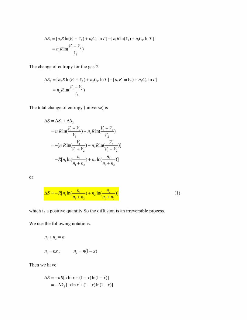
)]ln()ln([21

22

21

11

nn

nn

nn

nnRS

(1)

which is a positive quantity So the diffusion is an irreversible process.

We use the following notations.

nnn 21

nxn 1 , )1(2 xnn

Then we have

)]1ln()1(ln[[

)]1ln()1(ln[

xxxxNk

xxxxnRS

B

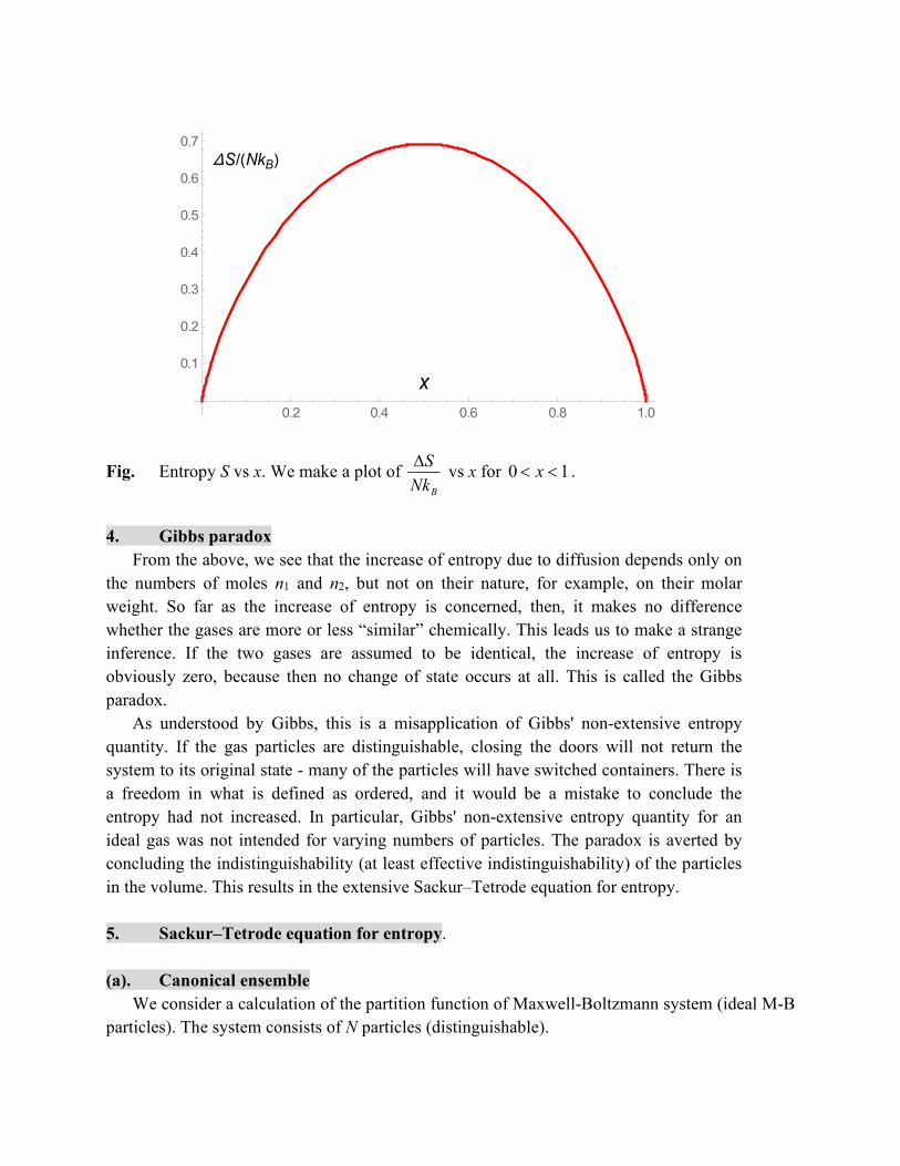
Fig. Entropy S vs x. We make a plot of B

S

Nk

vs x for 0 1x .

4. Gibbs paradox

From the above, we see that the increase of entropy due to diffusion depends only on

the numbers of moles n1 and n2, but not on their nature, for example, on their molar

weight. So far as the increase of entropy is concerned, then, it makes no difference

whether the gases are more or less “similar” chemically. This leads us to make a strange

inference. If the two gases are assumed to be identical, the increase of entropy is

obviously zero, because then no change of state occurs at all. This is called the Gibbs

paradox.

As understood by Gibbs, this is a misapplication of Gibbs' non-extensive entropy

quantity. If the gas particles are distinguishable, closing the doors will not return the

system to its original state - many of the particles will have switched containers. There is

a freedom in what is defined as ordered, and it would be a mistake to conclude the

entropy had not increased. In particular, Gibbs' non-extensive entropy quantity for an

ideal gas was not intended for varying numbers of particles. The paradox is averted by

concluding the indistinguishability (at least effective indistinguishability) of the particles

in the volume. This results in the extensive Sackur–Tetrode equation for entropy.

5. Sackur–Tetrode equation for entropy.

(a). Canonical ensemble

We consider a calculation of the partition function of Maxwell-Boltzmann system (ideal M-B

particles). The system consists of N particles (distinguishable).

S NkB

x

0.2 0.4 0.6 0.8 1.0

0.1

0.2

0.3

0.4

0.5

0.6

0.7

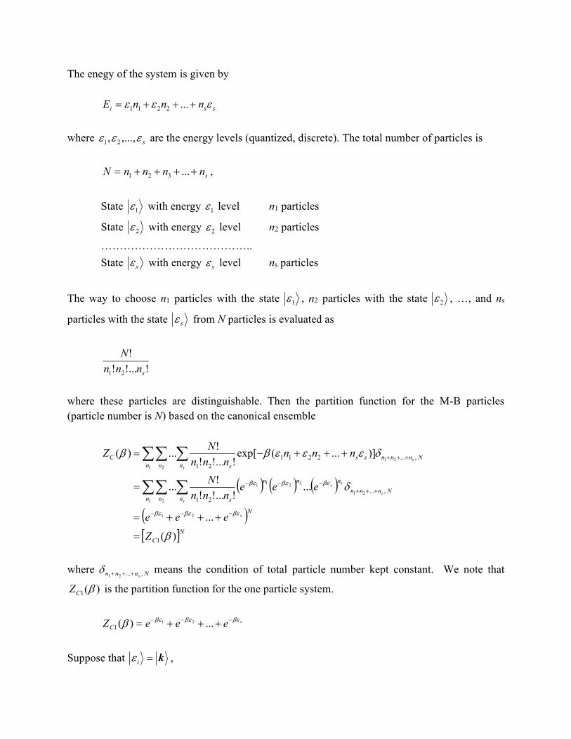
The enegy of the system is given by

ssi nnnE ...2211

where s ,...,, 21 are the energy levels (quantized, discrete). The total number of particles is

snnnnN ...321 ,

State 1 with energy 1 level n1 particles

State 2 with energy 2 level n2 particles

…………………………………..

State s with energy s level ns particles

The way to choose n1 particles with the state 1 , n2 particles with the state 2 , …, and ns

particles with the state s from N particles is evaluated as

!!...!

!

21 snnn

N

where these particles are distinguishable. Then the partition function for the M-B particles

(particle number is N) based on the canonical ensemble

NC

N

n n n

Nnnn

nnn

s

n n n

Nnnnss

s

C

Z

eee

eeennn

N

nnnnnn

NZ

s

s

s

ss

s

s

)(

...

...!!...!

!...

)]...(exp[!!...!

!...)(

1

,...

21

,...2211

21

21

1 2

21

22

11

1 2

21

where Nnnn s ,...21 means the condition of total particle number kept constant. We note that

)(1 CZ is the partition function for the one particle system.

seeeZC

...)( 21

1

Suppose that ki ,

m2

22k

k

ℏ

instead of i .

kkkH

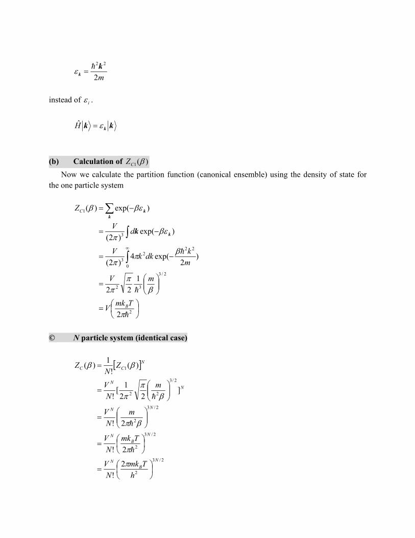
(b) Calculation of )(1 CZ

Now we calculate the partition function (canonical ensemble) using the density of state for

the one particle system

2

2/3

32

0

222

3

3

1

2

1

22

)2

exp(4)2(

)exp()2(

)exp()(

ℏ

ℏ

ℏ

TmkV

mV

m

kdkk

V

dV

Z

B

C

k

k

k

k

© N particle system (identical case)

2/3

2

2/3

2

2/3

2

2/3

22

1

2

!

2!

2!

]22

1[

!

)(!

1)(

N

B

N

N

B

N

NN

NN

N

CC

h

Tmk

N

V

Tmk

N

V

m

N

V

m

N

V

ZN

Z

ℏ

ℏ

ℏ

Note that

2/332 )2(

1

8

1

22

1

,

2h

ℏ

The Helmholtz free energy:

)]2

ln(2

31ln

2

3[ln

)]2

ln(2

3ln

2

3lnln[

)]2

ln(2

3ln

2

3!lnln[

),,(ln

2

2

2

h

mkT

N

VTNk

h

mkNT

NNNNVNTk

h

mkNT

NNVNTk

VTZTkF

BB

BB

BB

CB

or

)]2

ln(2

31ln

2

3[ln

2h

mkT

N

VTNkF B

B

),,(ln VTZ C is obtained as

)]2

ln(2

31ln

2

3[ln),,(ln

2h

mkT

N

VNVTZ B

C

The average energy

TNk

Z

ZT

Tk

T

F

TTE

B

V

V

B

V

2

3

ln

ln2

2

or

TNkE B2

3

The heat capacity at constant volume:

B

V

V NkT

EC

2

3

For ANN , we have RCV2

3 , where R is the gas constant. The heat capacity at constant

pressure is

RRCvCP2

5 , (Mayer’s relation)

The entropy S is

]2

5)

2ln(

2

3[ln

)]2

ln(2

31ln

2

3[ln

2

3

2

2

h

Tmk

N

VNk

h

mkT

N

VNkNk

T

FES

BB

BBB

or

]2

5)

2ln(

2

3[ln

2

h

Tmk

N

VNkS B

B

(Sackur–Tetrode equation)

The pressure P is

V

TNk

V

FP B

T

or

TNkPV B

8. Gibbs paradox (revisited)

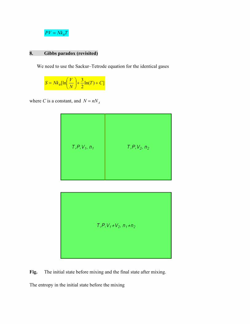
We need to use the Sackur–Tetrode equation for the identical gases

])ln(2

3[ln CT

N

VNkS B

where C is a constant, and AnNN

Fig. The initial state before mixing and the final state after mixing.

The entropy in the initial state before the mixing

])ln(2

3[ln)(

])ln(2

3[ln

])ln(2

3[ln

])ln(2

3[ln

])ln(2

3[ln

21

2

1

2

22

1

11

CTP

TkRnn

CTPN

RTRn

CTPN

RTRn

CTNn

VRn

CTNn

VRnS

B

A

A

A

A

i

since RTnPV 11 and RTnPV 22

CTNn

VRnS

A

i

)]ln(

2

3[ln

1

11

The entropy in the final state after the mixing is

])ln(2

3[ln)(

])ln(2

3[ln)(

])ln(2

3

)([ln)(

21

21

21

2121

CTP

TkRnn

CTPN

RTRnn

CTNnn

VVRnnS

B

A

A

f

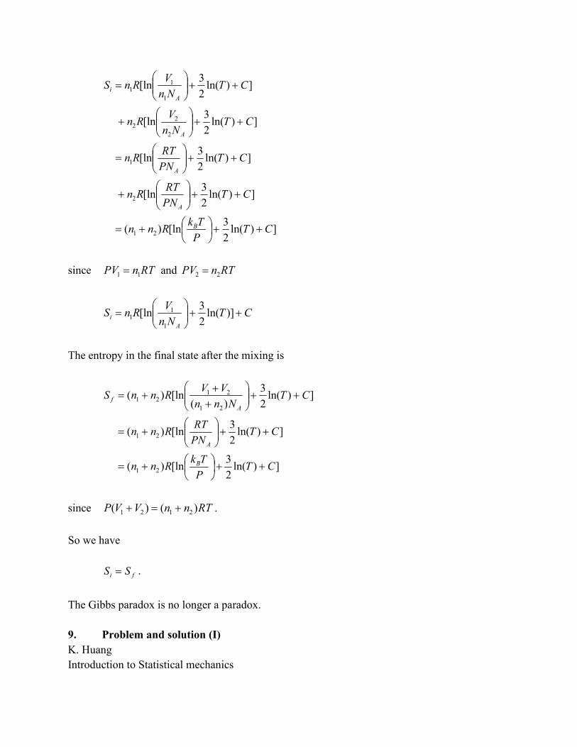
since RTnnVVP )()( 2121 .

So we have

fi SS .

The Gibbs paradox is no longer a paradox.

9. Problem and solution (I)

K. Huang

Introduction to Statistical mechanics

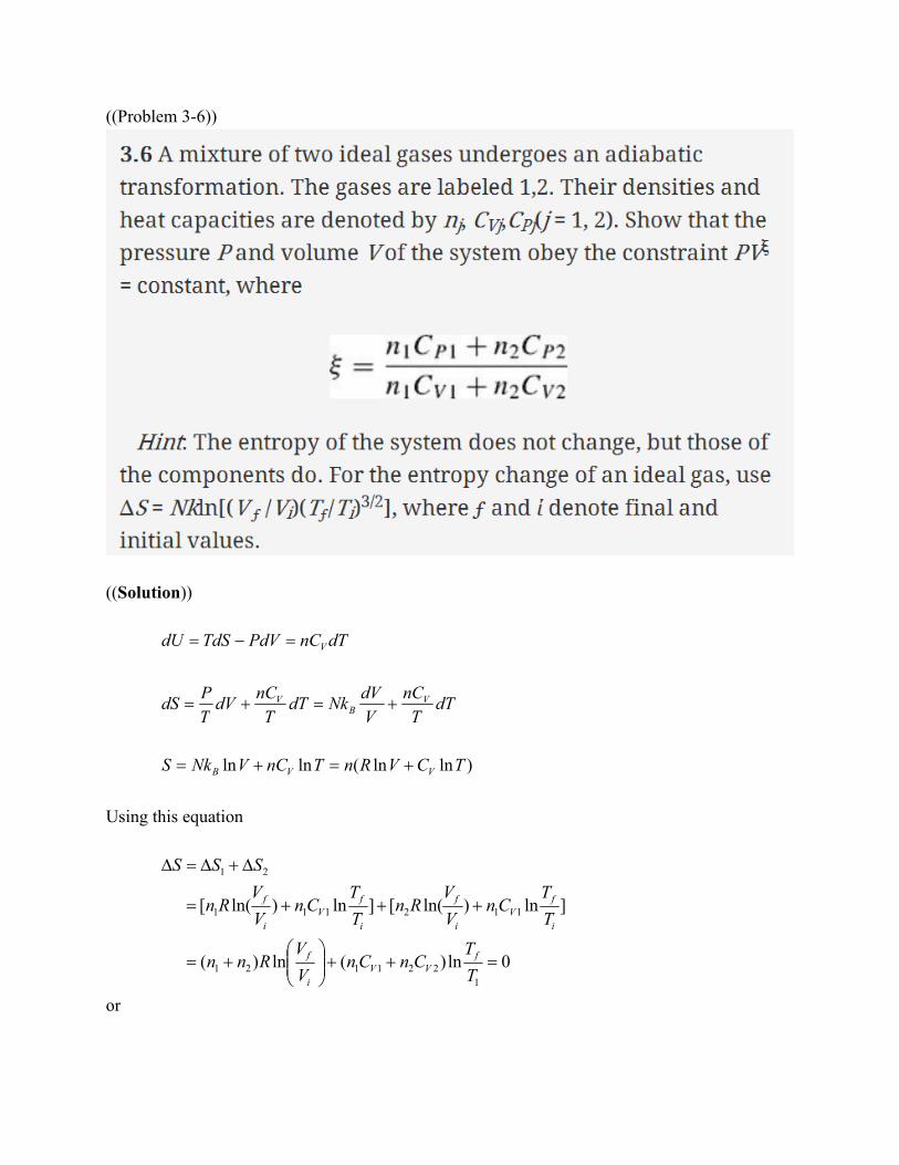
((Problem 3-6))

((Solution))

dTnCPdVTdSdU V

dTT

nC

V

dVNkdT

T

nCdV

T

PdS V

BV

)lnln(lnln TCVRnTnCVNkS VVB

Using this equation

0ln)(ln)(

]ln)ln([]ln)ln([

1

221121

112111

21

T

TCnCn

V

VRnn

T

TCn

V

VRn

T

TCn

V

VRn

SSS

f

VV

i

f

i

f

V

i

f

i

f

V

i

f

or

0lnln)(

)(

12211

21

T

T

V

V

CnCn

Rnn f

i

f

VV

or

0lnln

i

f

i

f

V

V

T

T

where

)(

)(

2211

21

VV CnCn

Rnn

or

constantTV

Putting RTnnnRTPV )( 21

constantPV

where

2211

2211

2211

221121

2211

21

)()(

)(

)(1

1

VV

PP

VV

VV

VV

CnCn

CnCn

CnCn

CnCnRnn

CnCn

Rnn

______________________________________________________________________

REFERENCES

M. Planck, Theory of Heat (Macmillan, 1957).

R. Kubo, Thermodynamics: An Advanced Course with Problems and Solutions (North

Holland, 1968).

F. Reif, Fundamentals of Statistical and Thermal Physics (McGraw-Hill, 1965).

C. Kittel and H. Kroemer, Thermal Physics, second edition (W.H. Freeman, 1980).