Mixing Probabilities, Priors and Kernels via Entropy Pooling

www.garp.org D E C E M B E R 2 0 1 1 RISK PROFESSIONAL 32

T H E Q U A N T C L A S S R O O M B Y AT T I L I O M E U C C I

Mixing Probabilities, Priors and Kernels

via Entropy PoolingHow to emphasize certain historical scenarios for risk

and portfolio management, according to their similarity with the current market conditions.

he Fully Flexible Probabilities framework discussed in Meucci (2010) represents the multi-variate distribution f of an arbitrary set of risk drivers, X (X1,...,XN)´, non-parametrically in terms of scenario-proba-bility pairs, as follows:

where the joint scenarios can be historical realizations or the outcome of simulations. The use of Fully Flexible Probabilities permits all sorts of manipula-tions of distributions essential for risk and portfolio manage-ment, such as pricing and aggregation (see Meucci, 2011) and the estimate of portfolio risk from these distributions.

The probabilities in the Fully Flexible Probabilities frame-work (1) can be set by crisp conditioning, kernel smoothing, ex-ponential time decay, etc. (see Figure 1, right).

(1)

Figure 1: Fully Flexible Probabilities Specification via Entropy Pooling

Another approach to set the probabilities in (1) is based on the Entropy Pooling technique by Meucci (2008). Entropy Pooling is a generalized Bayesian approach to process views on the market. It starts from two inputs, a prior market distri-bution, f0, and a set of generalized views or stress tests, , and yields a posterior distribution f that is close to the prior, but incorporates the views.

Entropy Pooling can be used in the non-parametric sce-

TMixing Probabilities, Priors and Kernels

via Entropy PoolingAttilio Meucci1

1 IntroductionThe Fully Flexible Probabilities framework discussed in Meucci (2010) repre-sents the multivariate distribution of an arbitrary set of risk drivers X ≡(1 )

0 non-parametrically in terms of scenario-probability pairs,

⇐⇒ {x }=1 , (1)

where the joint scenarios x ≡ (1 )0 can be historical realizations orthe outcome of simulations. The use of Fully Flexible Probabilities permits allsorts of manipulations of distributions essential for risk and portfolio manage-ment, such as pricing and aggregation, see Meucci (2011), and the estimate ofportfolio risk from these distributions.The probabilities in the Fully Flexible Probabilities framework (1) can be

set by crisp conditioning, kernel smoothing, exponential time decay, etc., referto Figure 1.Another approach to set the probabilities in (1) is based on the Entropy

Pooling technique by Meucci (2008). Entropy Pooling is a generalized Bayesianapproach to process views on the market. Entropy Pooling starts from twoinputs, a prior market distribution 0 and a set of generalized views or stress-tests V, and yields a posterior distribution that is close to the prior, butincorporates the views. Entropy Pooling can be used in the non-parametricscenario-probability representation of the Fully Flexible Probabilities framework(1), in which case it provides an optimal way to specify the probabilities p ≡(1 )

0 of the scenarios. Alternatively, Entropy Pooling can be used withparametric distributions that are fully specied by a set of parameters θ,such as the normal distribution.

1The author is grateful to Garli Beibi and David Elliott

1

Mixing Probabilities, Priors and Kernelsvia Entropy Pooling

Attilio Meucci1



⇐⇒ {x }=1 , (1)






1

Mixing Probabilities, Priors and Kernelsvia Entropy Pooling

Attilio Meucci1



⇐⇒ {x }=1 , (1)






1

33 RISK PROFESSIONAL D E C E M B E R 2 0 1 1 www.garp.org www.garp.org D E C E M B E R 2 0 1 1 RISK PROFESSIONAL 34

nario-probability representation of the Fully Flexible Prob-abilities framework (1), in which case it provides an optimal way to specify the probabilities p (p1,...,pJ)´of the scenarios. Alternatively, it can be used with parametric distributions f that are fully specified by a set of parameters , such as the normal distribution.

In this article, we show that Entropy Pooling represents the most general approach to optimally specify the probabilities of the scenarios (1) and includes common approaches (such as kernel smoothing) as special cases, when the prior distribution f0 contains no information. We will also demonstrate how to use Entropy Pooling to overlay different kernels/signals to an informative prior in a statistically sound way.

The remainder of the article will proceed as follows. In Section 2, we review common approaches to assign prob-abilities in (1) and we generalize such approaches using fuzzy membership functions.

In Section 3, we review the non-parametric implementa-tion of Entropy Pooling. Furthermore, we show how Entropy Pooling includes fuzzy membership probabilities. Finally, we discuss how to leverage Entropy Pooling to mix the above ap-proaches and overlay prior information to different estima-tion techniques.

In Section 4, we present a risk management case study, where we model the probabilities of the historical simulations of a portfolio P&L. Using Entropy Pooling we overlay to an exponentially time-decayed prior a kernel that modulates the probabilities according to the current state of implied volatil-ity and interest rates.

Time/State Conditioning and Fuzzy MembershipHere we review a few popular methods to specify the prob-abilities in the Fully Flexible Probabilities framework (1) ex-ogenously. For applications of these methods to risk manage-ment, refer to Meucci (2010).

If the scenarios are historical and we are at time T, a simple approach to specify probabilities exogenously is to discard old data and rely only on the most recent window of time . This entails setting the probabilities in (1), as follows:

An approach to assign weights to historical scenarios dif-ferent from the rolling window (2) is exponential smoothing

given set χ. Using a fuzzy membership mx for a given set χ of potential

market outcomes for the market χ, we can set the probability of each scenario as proportional to the degree of membership of that scenario to the set of outcomes

A trivial example of membership function is the following indicator function, which defines crisp conditioning (4):

With the indicator function, membership is either maximal and equal to 1, if x belongs to χ, or minimal and equal to 0, if x does not belong to χ.

A second example of membership function is the kernel (5), which is a membership function for the singleton χ

The membership of x to is maximal when x is . The larger the distance d of x from , the less x "belongs" to , and thus the closer to 0 the membership of x.

Entropy PoolingThe probability specification (8) assumes no prior knowledge of the distribution of the market risk drivers X. In this case, fuzzy membership is the most general approach to assign probabilities to the scenarios in (1). Here, we show how non-parametric Entropy Pooling further generalizes fuzzy mem-bership specifications to the case when prior information is available, or when we must blend together more than one membership specification.

First, we review the non-parametric Entropy Pooling imple-mentation. (Please refer to the original article Meucci (2008) for more details and more generality, as well as for the code.)

The starting point for non-parametric Entropy Pooling is a prior distribution f (0) for the risk drivers X, represented as in (1) by a set of scenarios and associated probabilities, as fol-lows:

The second input is a view on the market X, or a stress-

test. Thus, a generalized view on X is a statement on the yet-to-be-defined distribution defined on the same scenarios A large class of such views can be characterized as expressions on the expectations of arbitrary functions of the market v(X), as follows:

where v* is a threshold value that determines the intensity of the view.

To illustrate a typical view, consider the standard views, a la Black and Litterman (1990), on the expected value aX of select portfolios returns aX, where X represents the returns of N securities, and a is a K x N matrix, whose each row are the weights of a different portfolio. Such view can be written as in (12), where

Our ultimate goal is to compute a posterior distribution f that departs from the prior to incorporate the views. The posterior distribution f is specified by new probabilities p on the same scenarios (11). To this purpose, we measure the "dis-tance" between two sets of probabilities p and p0 by the rela-tive entropy

The relative entropy is a "distance" in that (13) is zero only if p = p0, and it becomes larger as p diverges away from p0. We then define the posterior as the closest distribution to the prior, as measured by (13), which satisfies the views (12), as follows:

where the notation p means that p satisfies the view (12).Applications of Entropy Pooling to the probabilities in the

Fully Flexible Probabilities framework are manifold. For in-stance, with Entropy Pooling, we can compute exponentially decayed covariances where the correlations and the variances are decayed at different rates. Other applications include con-ditioning the posterior according to expectations on a market panic indicator. (For more details see Meucci, 2010.)

As highlighted in Figure 1, the Entropy Pooling posterior (14) also includes as special cases the probabilities defined in terms of fuzzy membership functions (8). Indeed, let us as-sume that in the Entropy Pooling optimization (14), the prior

where > 0 is a given half-life for the decay.

An approach to assigning probabilities related to the rolling window (2) that does not depend on time, but rather on state, is crisp conditioning: the probabilities are set as non-null, and all equal, as long as the scenarios of the market drivers xj lie in a given domain χ. Using the indicator function 1χ (x), which is 1 if x X and 0 otherwise, we obtain

An enhanced version of crisp conditioning for assigning probabilities, related to the rich literature on machine learn-ing, is kernel smoothing. First, we recall that a kernel k (x) is defined by a positive non-increasing generator function k(d) [0.1], a target , a distance function d (x,y) and a radius, or bandwidth, , as follows:

For example, the Gaussian kernel reads

where the additional parameter is a symmetric, positive def-inite matrix. The Gaussian kernel (6) is in the form (5), where d is the Mahalanobis distance

Using a kernel we can condition the market variables X smoothly, by setting the probability of each scenario as pro-portional to the kernel evaluated on that scenario, as follows:

As we show in Appendix A.1, available at http://symmys.com/node/353, the crisp state conditioning (4) includes the rolling window (2) as a special case, and kernel smoothing (7) includes the time-decayed exponential smoothing (3) as a spe-cial case (see Figure 1).

We can generalize further the concepts of crisp condition-ing and kernel smoothing by means of fuzzy membership functions. Fuzzy membership to a given set χ is defined in terms of a "membership" function mχ(x) with values in the range [0,1], which describes to what extent x belongs to a

T H E Q U A N T C L A S S R O O M B Y AT T I L I O M E U C C I T H E Q U A N T C L A S S R O O M B Y AT T I L I O M E U C C I

2 Time/state conditioning and fuzzy member-ship

Here we review a few, popular methods to exogenously specify the probabilitiesin the Fully Flexible Probabilities framework (1). For applications of thesemethods to risk management, refer to Meucci (2010).If the scenarios are historical and we are at time , a simple approach to

exogenously specify probabilities is to discard old data and rely only on themost recent window of time . This entails setting the probabilities in (1) asfollows

∝½1 if − 0 otherwise.

. (2)

An approach to assign weights to historical scenarios different from therolling window (2) is exponential smoothing

∝ −ln 2 |− |, (3)

where 0 is a given half-life for the decay.An approach to assigning probabilities related to the rolling window (2)

that does not depend on time, but rather on state, is crisp conditioning: theprobabilities are set as non-null, and all equal, as long as the scenarios of themarket drivers x lie in a given domain X . Using the indicator function 1X (x),which is 1 if x ∈ X and 0 otherwise, we obtain

∝ 1X (x) (4)

An enhanced version of crisp conditioning for assigning probabilities, relatedto the rich literature on machine learning, is kernel smoothing. First, we recallthat a kernel (x) is dened by a positive non-increasing generator function () ∈ [0 1], a target μ, a distance function (xy), and a radius, or bandwidth, as follows

(x) ≡ ( (xμ)

). (5)


(x) ≡ −122(x−)0−1(x−), (6)

where the additional parameter σ is a symmetric, positive denite matrix. TheGaussian kernel (6) is in the form (5), where is the Mahalanobis distance2 (xμ) ≡ (x− μ)0 σ−1 (x− μ).Using a kernel we can condition the market variables X smoothly, by setting

the probability of each scenario as proportional to the kernel evaluated on thatscenario

∝ (x). (7)

3

(2)





. (2)


∝ −ln 2 |− |, (3)



∝ 1X (x) (4)


(x) ≡ ( (xμ)

). (5)


(x) ≡ −122(x−)0−1(x−), (6)



∝ (x). (7)

3





. (2)


∝ −ln 2 |− |, (3)



∝ 1X (x) (4)


(x) ≡ ( (xμ)

). (5)


(x) ≡ −122(x−)0−1(x−), (6)



∝ (x). (7)

3





. (2)


∝ −ln 2 |− |, (3)



∝ 1X (x) (4)


(x) ≡ ( (xμ)

). (5)


(x) ≡ −122(x−)0−1(x−), (6)



∝ (x). (7)

3





. (2)


∝ −ln 2 |− |, (3)



∝ 1X (x) (4)


(x) ≡ ( (xμ)

). (5)


(x) ≡ −122(x−)0−1(x−), (6)



∝ (x). (7)

3





. (2)


∝ −ln 2 |− |, (3)



∝ 1X (x) (4)


(x) ≡ ( (xμ)

). (5)


(x) ≡ −122(x−)0−1(x−), (6)



∝ (x). (7)

3





. (2)


∝ −ln 2 |− |, (3)



∝ 1X (x) (4)


(x) ≡ ( (xμ)

). (5)


(x) ≡ −122(x−)0−1(x−), (6)



∝ (x). (7)

3

(4)

(5)

(6)

(7)

As we show in Appendix A.1, available at http://symmys.com/node/353,the crisp state conditioning (4) includes the rolling window (2) as a special case,and kernel smoothing (7) includes the time decayed exponential smoothing (3)as a special case, see Figure 1.We can generalize further the concepts of crisp conditioning and kernel

smoothing by means of fuzzy membership functions. Fuzzy membership to agiven set X is dened in terms of a "membership" function X (x) with valuesin the range [0 1], which describes to what extent x belongs to a given set X .Using a fuzzy membership X for a given set X of potential market outcomesfor the market X, we can set the probability of each scenario as proportional tothe degree of membership of that scenario to the set of outcomes

∝ X (x). (8)

A trivial example of membership function is the indicator function thatdenes crisp conditioning (4)

X (x) ≡ 1X (x) . (9)

With the indicator function, membership is either maximal, and equal to 1, ifx belongs to X , or minimal, and equal to 0, if x does not belong to X .A second example of membership function is the kernel (5), which is a mem-

bership function for the singleton X ≡ μ

(x) ≡ (x) . (10)

The membership of x to μ is maximal when x is μ. The larger the distance of x from μ, the less x "belongs" to μ and thus the closer to 0 the membershipof x.

3 Entropy PoolingThe probability specication (8) assumes no prior knowledge of the distributionof the market risk drivers X. In this case, fuzzy membership is the most generalapproach to assign probabilities to the scenarios in (1). Here we show how non-parametric Entropy Pooling further generalizes fuzzy membership specicationsto the case when prior information is available, or when we must blend togethermore than one membership specication.First, we review the non-parametric Entropy Pooling implementation. Please

refer to the original article Meucci (2008) for more details, more generality, andfor the code.The starting point for non-parametric Entropy Pooling is a prior distribution

(0) for the risk drivers X, represented as in (1) by a set of scenarios andassociated probabilities

0 ⇐⇒ {x (0) }=1 . (11)

4



∝ X (x). (8)


X (x) ≡ 1X (x) . (9)



(x) ≡ (x) . (10)





0 ⇐⇒ {x (0) }=1 . (11)

4



∝ X (x). (8)


X (x) ≡ 1X (x) . (9)



(x) ≡ (x) . (10)





0 ⇐⇒ {x (0) }=1 . (11)

4



∝ X (x). (8)


X (x) ≡ 1X (x) . (9)



(x) ≡ (x) . (10)





0 ⇐⇒ {x (0) }=1 . (11)

4

The second input is a view on the market X, or a stress-test. Thus a gen-eralized view on X is a statement on the yet-to-be dened distribution denedon the same scenarios ⇐⇒ {x }=1 . A large class of such views canbe characterized as expressions on the expectations of arbitrary functions of themarket (X).

V : Ep { (X)} ≥ ∗, (12)

where ∗ is a threshold value that determines the intensity of the view.To illustrate a typical view, consider the standard views a-la Black and

Litterman (1990) on the expected value μaX of select portfolios returns aX,where X represents the returns of securities, and a is a × matrix, whoseeach row are the weights of a different portfolio. Such view can be written as in(12), where (X) ≡ (a0−a0)0 and ∗ ≡ (μaX−μ0aX)0.Our ultimate goal is to compute a posterior distribution which departs

from the prior to incorporate the views. The posterior distribution is speciedby new probabilities p on the same scenarios (11). To this purpose, we measurethe "distance" between two sets of probabilities p and p0 by the relative entropy

E (pp0) ≡ p0 (lnp− lnp0) . (13)

The relative entropy is a "distance" in that (13) is zero only if p = p0 and itbecomes larger as p diverges away from p0.Then we dene the posterior as the closest distribution to the prior, as

measured by (13), which satises the views (12)

p ≡ argminq∈V

E (qp0) , (14)

where the notation p ∈ V means that p satises the view (12).Applications of Entropy Pooling to the probabilities in the Fully Flexible

Probabilities framework are manifold. For instance, with Entropy Pooling, wecan compute exponentially decayed covariances where the correlations and thevariances are decayed at different rates. Other applications include conditioningthe posterior according to expectations on a market panic indicator. For moredetails see Meucci (2010).As highlighted in Figure 1, the Entropy Pooling posterior (14) also includes

as special cases the probabilities dened in terms of fuzzy membership functions(8). Indeed, let us assume that in the Entropy Pooling optimization (14) theprior is non-informative, i.e.

p0 ∝ 1. (15)

Furthermore, let us assume that in the Entropy Pooling optimization (14) weexpress the view (12) on the logarithm of a fuzzy membership functionX (x) ∈[0 1]

(x) ≡ ln (X (x)) . (16)

Finally, let us set the view intensity in (12) as

∗ ≡P

=1X (x) lnX (x)P

=1X (x)

. (17)

5


V : Ep { (X)} ≥ ∗, (12)




E (pp0) ≡ p0 (lnp− lnp0) . (13)



p ≡ argminq∈V

E (qp0) , (14)




p0 ∝ 1. (15)


(x) ≡ ln (X (x)) . (16)


∗ ≡P

=1X (x) lnX (x)P

=1X (x)

. (17)

5


V : Ep { (X)} ≥ ∗, (12)




E (pp0) ≡ p0 (lnp− lnp0) . (13)



p ≡ argminq∈V

E (qp0) , (14)




p0 ∝ 1. (15)


(x) ≡ ln (X (x)) . (16)


∗ ≡P

=1X (x) lnX (x)P

=1X (x)

. (17)

5

(12)The second input is a view on the market X, or a stress-test. Thus a gen-

eralized view on X is a statement on the yet-to-be dened distribution denedon the same scenarios ⇐⇒ {x }=1 . A large class of such views canbe characterized as expressions on the expectations of arbitrary functions of themarket (X).

V : Ep { (X)} ≥ ∗, (12)




E (pp0) ≡ p0 (lnp− lnp0) . (13)



p ≡ argminq∈V

E (qp0) , (14)




p0 ∝ 1. (15)


(x) ≡ ln (X (x)) . (16)


∗ ≡P

=1X (x) lnX (x)P

=1X (x)

. (17)

5


V : Ep { (X)} ≥ ∗, (12)




E (pp0) ≡ p0 (lnp− lnp0) . (13)



p ≡ argminq∈V

E (qp0) , (14)




p0 ∝ 1. (15)


(x) ≡ ln (X (x)) . (16)


∗ ≡P

=1X (x) lnX (x)P

=1X (x)

. (17)

5

(3)

(9)

(8)

(10)

(11)

(13)

(14)

35 RISK PROFESSIONAL D E C E M B E R 2 0 1 1 www.garp.org www.garp.org D E C E M B E R 2 0 1 1 RISK PROFESSIONAL 36

is non-informative -- i.e.,

Furthermore, let us assume that in the Entropy Pooling opti-mization (14) we express the view (12) on the logarithm of a fuzzy membership function mx (x) [0,1] as


Then, as we show in Appendix A.2, available at http://sym-mys.com/node/353, the Entropy Pooling posterior (14) reads

This means that, without a prior, the Entropy Pooling poste-rior is the same as the fuzzy membership function, which in turn is a general case of kernel smoothing and crisp condi-tioning (see also the examples in Appendix A.3, available at http://symmys.com/node/353).

Not only does Entropy Pooling generalize fuzzy member-ship, it also allows us to blend multiple views with a prior. Indeed, let us suppose that, unlike in (15), we have an infor-mative prior p(0) on the market X — such as, for instance, the exponential time decay predicate (3) — that recent infor-mation is more reliable than old information. Suppose also that we would like to condition our distribution of the market based on the state of the market using a membership function as in (18) — such as, for instance, a Gaussian kernel. How do we mix these two conflicting pieces of information?

Distributions can be blended in a variety of ad-hoc ways. Entropy Pooling provides a statistically sound answer: we sim-ply replace the non-informative prior (15) with our informa-tive prior p(0) in the Entropy Pooling optimization (14) driven by the view (12) on the log-membership function (16) with intensity (17). In summary, the optimal blend reads

More generally, we can add to the view in (19) other views

on different features of the market distribution (as in Meucci, 2008).

It is worth emphasizing that all the steps of the above process are computationally trivial, from setting the prior p(0) to setting the constraint on the expectation, to computing the posterior (19). Thus the Entropy Pooling mixture is also practical.

Case Study: Conditional Risk EstimatesHere we use Entropy Pooling to mix information on the dis-tribution of a portfolio’s historical simulations. A standard approach to risk management relies on so-called historical simulations for the portfolio P&L: current positions are evalu-ated under past realizations {xt}t=1,...,T of the risk drivers X, giving rise to a history of {xt}t=1,...,T. To estimate the risk in the portfolio, one can assign equal weight to all the realiza-tions. The more versatile Fully Flexible Probability approach (1) allows for arbitrary probability weights

Refer to Meucci, 2010, for more details.

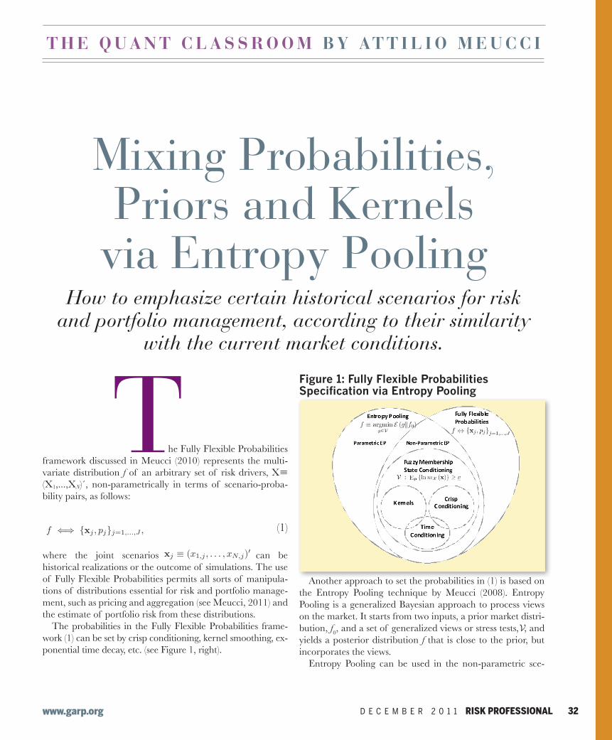
In our case study we consider a portfolio of options, whose historically simulated daily P&L distribution over a period of ten years is highly skewed and kurtotic, and definitely non-normal. Using Fully Flexible Probabilities, we model the ex-ponential decay prior that recent observations are more rel-evant for risk estimation purposes

where, is a half-life of 120 days. We plot these probabilities in the top portion of Figure 2 (below).

Figure 2: Mixing Distributions via Entropy Pooling

We condition the market on two variables: the five-year swap rate, which we denote by X1, and the one-into-five swaption implied at-the-money volatility, which we denote by X2. We estimate the 2 x 2 covariance matrix of these variables, and we construct a quasi-Gaussian kernel, similar to (6), setting as target the current values xT of the conditioning variables

In this expression, the bandwidth 10 and 0.4 is a power for the Mahalanobis distance, which allows for a smoother conditioning than =2.

If we used directly the membership levels (22) as probabili-ties pt mt, we would disregard the prior information (21) that more recent data is more valuable for our analysis. If we used only the exponentially decayed prior (21), we would disregard all the information conditional on the market state (22). To overlay the conditional information to the prior, we compute the Entropy Pooling posterior (19), which we write here

Notice that for each specification of the kernel bandwidth and radius depth in (22) we obtain a different posterior. Hence, a further refinement of the proposed approach lets the data determine the optimal bandwidth, by minimizing the relative entropy in (23) as a function of q as well as (,). We leave this step to the reader.

The kernel-based posterior (23) can be compared with al-ternative uses of Entropy Pooling to overlay a prior with par-tial information. For instance, Meucci (2010) obtains the pos-terior by imposing that the expected value of the conditioning variables be the same as the current value, i.e. Eq{X} =xT.

This approach is reasonable in a univariate context. How-ever, when the number of conditioning variables X is larger than one, due to the curse of dimensionality, we can obtain the undesirable result that the posterior probabilities are highly concentrated in a few extreme scenarios. This does not happen if we condition through a pseudo-Gaussian kernel as in (22)-(23)

In Figure 2 (see pg. 34), we plot the Entropy Pooling poste-rior probabilities (23) in our example. We can appreciate the hybrid nature of these probabilities, which share similarities with both the prior (21) and the conditioning kernel (22).

Using the Entropy Pooling posterior probabilities (23), we can perform all sorts of risk computations, as in Meucci (2010). In (24) we present a few significant statistics for our historical portfolio (20), and we compare such statistics with those stemming from the standard exponential decay (21) and the standard conditioning kernel (22). For more details, we refer the reader to the code available at http://symmys.com/node/353.

On the last row of (24) we also report the effective num-ber of scenarios, a practical measure of the predictive power of the above choices of probabilities, discussed in detail in Meucci (2012).

ReferencesBlack, F. and R. Litterman, 1990. "Asset allocation: Combining Investor Views with Market Equilibrium," Goldman Sachs Fixed Income Research.

Meucci, A., 2008. "Fully Flexible Views: Theory and Practice," Risk 21, 97—102. Article and code available at http://symmys.com/node/158.

ibid, 2010. "Historical scenarios with Fully Flexible Probabilities," Risk Professional December, 40—43. Article and code available at http://symmys.com/node/150.

ibid, 2011. "The Prayer: Ten-step Checklist for Advanced Risk and Portfolio Management," Risk Professional April/June, 54—60/55—59. Available at http://symmys.com/node/63.

ibid, 2012. "Effective Number of Scenarios with Fully Flexible Probabilities," Working Paper article and code available at http://symmys.com/node/362.

Attilio Meucci is the chief risk officer at Kepos Capital LP. He runs the 6-day "Ad-vanced Risk and Portfolio Management Bootcamp," see www.symmys.com. He is grateful to Garli Beibi and David Elliott.

T H E Q U A N T C L A S S R O O M B Y AT T I L I O M E U C C I T H E Q U A N T C L A S S R O O M B Y AT T I L I O M E U C C I


V : Ep { (X)} ≥ ∗, (12)




E (pp0) ≡ p0 (lnp− lnp0) . (13)



p ≡ argminq∈V

E (qp0) , (14)




p0 ∝ 1. (15)


(x) ≡ ln (X (x)) . (16)


∗ ≡P

=1X (x) lnX (x)P

=1X (x)

. (17)

5


V : Ep { (X)} ≥ ∗, (12)




E (pp0) ≡ p0 (lnp− lnp0) . (13)



p ≡ argminq∈V

E (qp0) , (14)




p0 ∝ 1. (15)


(x) ≡ ln (X (x)) . (16)


∗ ≡P

=1X (x) lnX (x)P

=1X (x)

. (17)

5


V : Ep { (X)} ≥ ∗, (12)




E (pp0) ≡ p0 (lnp− lnp0) . (13)



p ≡ argminq∈V

E (qp0) , (14)




p0 ∝ 1. (15)


(x) ≡ ln (X (x)) . (16)


∗ ≡P

=1X (x) lnX (x)P

=1X (x)

. (17)

5

(15)

(16)

(17)

(18)

Then, as we show in Appendix A.2, available at http://symmys.com/node/353,the Entropy Pooling posterior (14) reads

∝ X (x). (18)

This means that, without a prior, the Entropy Pooling posterior is the same asthe fuzzy membership function, which in turn is a general case of kernel smooth-ing and crisp conditioning, see also the examples in Appendix A.3, available athttp://symmys.com/node/353.Not only does Entropy Pooling generalize fuzzy membership, it also allows

us to blend multiple views with a prior. Indeed, let us suppose that, unlike in(15), we have an informative prior p(0) on the market X, such as for instancethe exponential time decay predicate (3) that recent information is more reli-able than old information. Suppose also that we would like to condition ourdistribution of the market based on the state of the market using a membershipfunction as in (18), such as for instance a Gaussian kernel. How do we mix thesetwo conicting pieces of information?Distributions can be blended in a variety of ad-hoc ways. Entropy Pooling

provides a statistically sound answer: we simply replace the non-informativeprior (15) with our informative prior p(0) in the Entropy Pooling optimization(14) driven by the view (12) on the log-membership function (16) with intensity(17). In summary, the optimal blend reads

p ≡ argminqE(qp(0)). (19)

where Eq {ln (X (X))} ≥ ∗.

More in general, we can add to the view in (19) other views on different featuresof the market distribution, as in Meucci (2008).It is worth emphasizing that all the steps of the above process are com-

putationally trivial, from setting the prior p(0) to setting the constraint on theexpectation, to computing the posterior (19). Thus the Entropy Pooling mixtureis also practical.

4 Case study: conditional risk estimatesHere we use Entropy Pooling to mix information on the distribution of a port-folio’s historical simulations. A standard approach to risk management relieson so-called historical simulations for the portfolio P&L: current positions areevaluated under past realizations {x}=1 of the risk drivers X, giving riseto a history of P&L’s {}=1 . To estimate the risk in the portfolio, onecan assign equal weight to all the realizations. The more versatile Fully FlexibleProbability approach (1) allows for arbitrary probability weights

⇐⇒ {(x) }=1 , (20)

refer to Meucci (2010) for more details.

6


∝ X (x). (18)









⇐⇒ {(x) }=1 , (20)


6


∝ X (x). (18)









⇐⇒ {(x) }=1 , (20)


6

In our case study we consider a portfolio of options, whose historically simu-lated daily P&L distribution over a period of ten years is highly skewed and kur-totic, and denitely non-normal. Using Fully Flexible Probabilities, we modelthe exponential decay prior that recent observations are more relevant for riskestimation purposes

(0) ∝ −

ln 2 (−), (21)

where, is a half-life of 120 days. We plot these probabilities in the top portionof Figure 2.

Prior (exponential time decay)

State indicator (2yr swap rate ‐ current level)

Membership (Gaussian kernel)

Posterior (Entropy Pooling mixture)

time

State indicator (1>5yr ATM implied swaption vol ‐ current level)

Figure 2: Mixing distributions via Entropy Pooling

Then we condition the market on two variables: the ve-year swap rate,which we denote by 1, and the one-into-ve swaption implied at-the-moneyvolatility, which we denote by 2. We estimate the 2×2 covariance matrix σ ofthese variables, and we construct a quasi-Gaussian kernel, similar to (6), settingas target the current values x of the conditioning variables

≡ exp(− 122

£(x − x )0 σ−1 (x − x )

¤). (22)

In this expression the bandwidth is ≈ 10 and ≈ 04 is a power for theMahalanobis distance, which allows for a smoother conditioning than = 2.If we used directly the membership levels (22) as probabilities ∝ ,

we would disregard the prior information (21) that more recent data is morevaluable for our analysis. If we used only the exponentially decayed prior (21),

7

(21)

In our case study we consider a portfolio of options, whose historically simu-lated daily P&L distribution over a period of ten years is highly skewed and kur-totic, and denitely non-normal. Using Fully Flexible Probabilities, we modelthe exponential decay prior that recent observations are more relevant for riskestimation purposes

(0) ∝ −

ln 2 (−), (21)

where, is a half-life of 120 days. We plot these probabilities in the top portionof Figure 2.


State indicator (2yr swap rate ‐ current level)



time

State indicator (1>5yr ATM implied swaption vol ‐ current level)

Figure 2: Mixing distributions via Entropy Pooling

Then we condition the market on two variables: the ve-year swap rate,which we denote by 1, and the one-into-ve swaption implied at-the-moneyvolatility, which we denote by 2. We estimate the 2×2 covariance matrix σ ofthese variables, and we construct a quasi-Gaussian kernel, similar to (6), settingas target the current values x of the conditioning variables

≡ exp(− 122

£(x − x )0 σ−1 (x − x )

¤). (22)

In this expression the bandwidth is ≈ 10 and ≈ 04 is a power for theMahalanobis distance, which allows for a smoother conditioning than = 2.If we used directly the membership levels (22) as probabilities ∝ ,

we would disregard the prior information (21) that more recent data is morevaluable for our analysis. If we used only the exponentially decayed prior (21),

7

(22)

we would disregard all the information conditional on the market state (22).To overlay the conditional information to the prior, we compute the EntropyPooling posterior (19), which we write here

p ≡ argminq0 lnm≥∗

E(qp(0)). (23)

Notice that for each specication of the kernel bandwidth and radius depth in(22) we obtain a different posterior. Hence, a further renement of the proposedapproach lets the data determine the optimal bandwidth, by minimizing therelative entropy in (23) as a function of q as well as ( ). We leave this step tothe reader.The kernel-based posterior (23) can be compared with alternative uses of En-

tropy Pooling to overlay a prior with partial information. For instance, Meucci(2010) obtains the posterior by imposing that the expected value of the con-ditioning variables be the same as the current value, i.e. Eq {X} = x . Thisapproach is reasonable in a univariate context. However, when the number ofconditioning variables X is larger than one, due to the curse of dimensionality,we can obtain the undesirable result that the posterior probabilities are highlyconcentrated in a few extreme scenarios. This does not happen if we conditionthrough a pseudo-Gaussian kernel as in (22)-(23)In Figure 2 we plot the Entropy Pooling posterior probabilities (23) in our

example. We can appreciate the hybrid nature of these probabilities, whichshare similarities with both the prior (21) and the conditioning kernel (22).

Time decay Kernel Entropy PoolingExp. value 0.12 0.05 0.10St. dev. 1.18 1.30 1.26Skew. -2.65 -2.56 -2.76Kurt. 12.58 11.76 13.39VaR 99% -4.62 -5.53 -5.11Cond. VaR 99% -6.16 -6.70 -6.85Effective scenarios 471 1,644 897

(24)

Using the Entropy Pooling posterior probabilities (23) we can perform all sortsof risk computations, as in Meucci (2010). In (24) we present a few signicantstatistics for our historical portfolio (20), and we compare such statistics withthose stemming from the standard exponential decay (21) and the standardconditioning kernel (22). For more details, we refer the reader to the codeavailable at http://symmys.com/node/353.On the last row of (24) we also report the effective number of scenarios, a

practical measure of the predictive power of the above choices of probabilities,discussed in detail in Meucci (2012).

ReferencesBlack, F., and R. Litterman, 1990, Asset allocation: combining investor viewswith market equilibrium, Goldman Sachs Fixed Income Research.

8

(23)

(24)


State indicator (2yr swap rate - current level)

State indicator (1>5yr ATM implied swaption vol - current level)



time

Timedecay Kernel EntropyPooling

Exp. value 0.12 0.05 0.10

St. dev. 1.18 1.30 1.26

Skew. -2.65 -2.56 -2.76

Kurt. 12.58 11.76 13.39

VaR 99% -4.62 -5.53 -5.11

Cond. VaR 99% -6.16 -6.70 -6.85

Effectivescenarios 47 11,644 897

(20)

(19)

37 RISK PROFESSIONAL D E C E M B E R 2 0 1 1 www.garp.org

T H E Q U A N T C L A S S R O O M B Y AT T I L I O M E U C C I

GARP Webcasts bring the risk profession’s top thought leaders and innovators direct to your desktop, so you can learn from their insights on the critical issues facing risk professionals today. GARP producesbetween fifteen and twenty live Webcasts each year. As a benefit of Membership, the US$49 fee per paid Webcast iswaived for GARP Individual and Student Members, who also receive unlimited access to the Webcast archive.

Upcoming Webcasts

w Risk Appetite, Governance and Corporate Strategy—Presented by SAS | December 6 >Register

w The Ramifications of Dodd-Frank: Consumer Protection | December 13 >Register

Featured On-Demand Webcasts

w The Ramifications of Dodd-Frank: The Volcker Rule >View

w The Ramifications of Dodd-Frank: Securitization >View

w The Ramifications of Dodd-Frank: Derivatives >View

w Using Operational Risk to Gain a Competitive Edge >View

A full selection of GARP Webcasts can be found at www.garp.org/webcasts

Creating a culture of risk awareness.TM

© 2011 Global Association of Risk Professionals. All rights reserved.

The world’s leading risk practitioners can now be found on your desktop.

Documents

Mixing Probabilities, Priors and Kernels via Entropy Pooling