1a 1b

Course Administration

Math Placement

Syllabus (show text)

WebAssign, class keys on syllabus

FDOC_self_enrollment.ppt

Your first homework assignment:

(1) self enroll in WebAssign

(2) Intro to WebAssign

(3) Math 171 week #1A

Due this Friday at 11:59pm for MW and TuTh

tutorials.

Due this Saturday at 11:59pm for WF tutorials.

First tutorial meeting this week is cancelled.

§1.1 Function Machines

sketch x [f] y = f(x), input, output

domain={possible inputs}

range={possible outputs}

x is the independent variable (represents an input

value)

y is the dependent variable (represents an output

value)

A function is a rule that assigns to each element in its

domain exactly one element in its range.

Example. 𝑓 𝑥 = 𝑥2, −1 ≤ 𝑥 ≤ 1. domain

= [−1,1]. range = [0,1]. ■

2a 2b

Interval Notation

𝑥 ∈ [−1,1] means −1 ≤ 𝑥 ≤ 1

𝑥 ∈ (−1,1) means −1 < 𝑥 < 1

𝑥 ∈ (−∞,∞) means 𝑥 is any real no.

Example. 𝑔 𝑥 = 𝑥2, domain = (−∞,∞).

range= [0, ∞). ■

If the domain of a function is not given explicitly,

assume it is the largest set of numbers that makes

sense.

Example. 𝑕 𝑥 = 𝑥, domain not given.

Assume domain= [0, ∞). range = [0,∞). ■

Graphs

Example. 𝑦 = 𝑥2

sketch …− 1 … 0 … 1 …𝑥- (independent variable),

0 …𝑦- (dependent variable), curve■

Example. 𝑦 = 𝑥

sketch 0 … 4 …𝑥-, 0 … 2 …𝑦-, curve■

3a 3b

Example. Graph the set of points that satisfy 𝑦2 = 𝑥.

Table x / 0, 1, 4; y/ 0, ±1, ±2

sketch 0 … 4 …𝑥-, −2 … 0 … 2 …𝑦-, curve

Is this a function?

?? Why? ■

Vertical Line Test

A curve in the xy-plane is the graph of a function iff

no vertical line intersects the curve more than once.

Example. Draw the graph of 𝑥2 + 𝑦2 = 1.

axes, circle, vertical line intersecting circle twice

?? Is this the graph of a function?

?? Why?

4a 4b

Even and odd symmetry

If 𝑓(𝑥) satisfies

𝑓 −𝑥 = 𝑓(𝑥)

for every 𝑥 in its domain, then 𝑓 is called an even

function.

Example. 𝑓 𝑥 = 𝑥2,

𝑓 −𝑥 = −𝑥 2 = −𝑥 −𝑥 = 𝑥2 = 𝑓(𝑥).

?? If 𝑓 is even, its graph is symmetric wrt which axis?

■

If 𝑔(𝑥) satisfies

𝑔 −𝑥 = −𝑔(𝑥)

for every 𝑥 in its domain, then 𝑔 is an odd function.

Example. 𝑔 𝑥 = 𝑥3,

𝑔 −𝑥 = −𝑥 −𝑥 −𝑥 = −𝑥3 = −𝑔(𝑥) .

Table x/ 0, -1, 1, -2, 2; y/ 0, -1, 1, -8, 8

sketch −2 … 0 … 2 …𝑥-, −8 … 0 … 8 …𝑦-, curve

?? If 𝑔 is odd, its graph is symmetric wrt what? ■

Knowing even or odd symmetry helps us sketch

functions.

5a 5b

§1.2 Catalog Of Functions

Straight lines

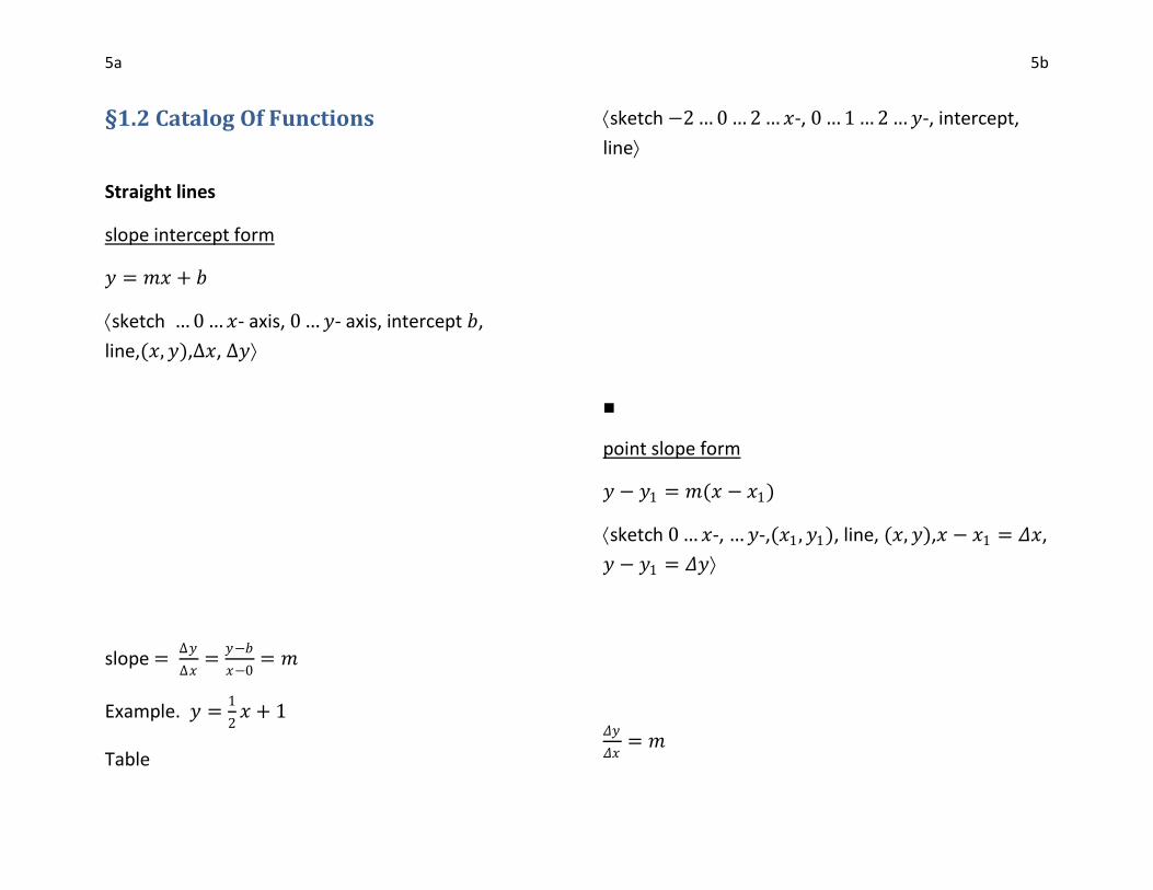
slope intercept form

𝑦 = 𝑚𝑥 + 𝑏

sketch … 0 …𝑥- axis, 0 …𝑦- axis, intercept 𝑏,

line,(𝑥, 𝑦),Δ𝑥, Δ𝑦

slope = Δ𝑦

Δ𝑥=

𝑦−𝑏

𝑥−0= 𝑚

Example. 𝑦 =1

2𝑥 + 1

Table

sketch −2 … 0 … 2 …𝑥-, 0 … 1 … 2 …𝑦-, intercept,

line

■

point slope form

𝑦 − 𝑦1 = 𝑚(𝑥 − 𝑥1)

sketch 0 …𝑥-, …𝑦-,(𝑥1, 𝑦1), line, (𝑥, 𝑦),𝑥 − 𝑥1 = 𝛥𝑥,

𝑦 − 𝑦1 = 𝛥𝑦

𝛥𝑦

𝛥𝑥= 𝑚

6a 6b

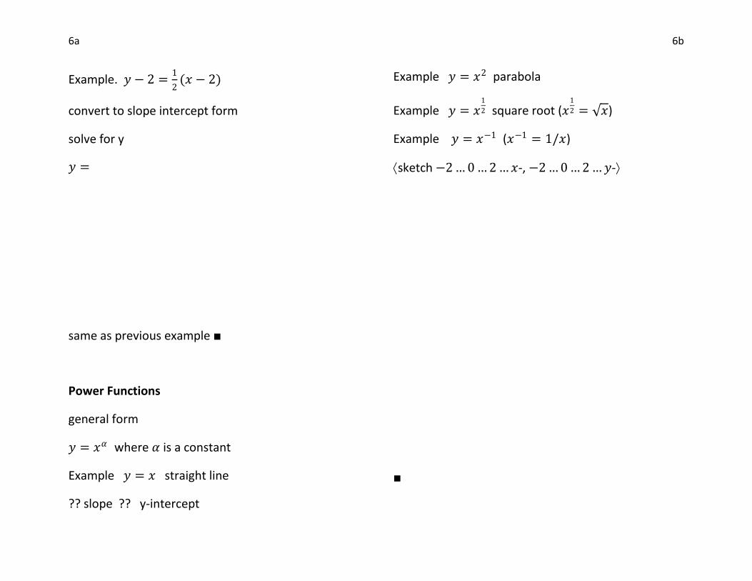
Example. 𝑦 − 2 =1

2(𝑥 − 2)

convert to slope intercept form

solve for y

𝑦 =

same as previous example ■

Power Functions

general form

𝑦 = 𝑥𝛼 where 𝛼 is a constant

Example 𝑦 = 𝑥 straight line

?? slope ?? y-intercept

Example 𝑦 = 𝑥2 parabola

Example 𝑦 = 𝑥1

2 square root (𝑥1

2 = 𝑥)

Example 𝑦 = 𝑥−1 (𝑥−1 = 1/𝑥)

sketch −2 … 0 … 2 …𝑥-, −2 … 0 … 2 …𝑦-

■

7a 7b

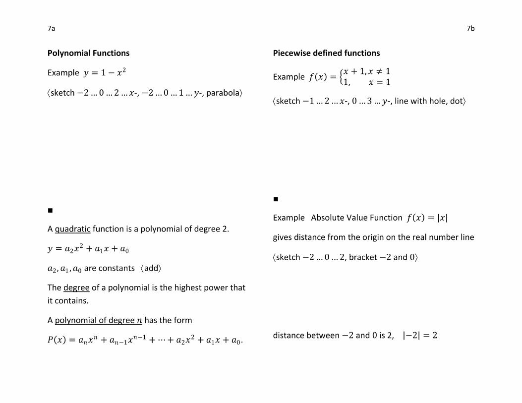
Polynomial Functions

Example 𝑦 = 1 − 𝑥2

sketch −2 … 0 … 2 …𝑥-, −2 … 0 … 1 …𝑦-, parabola

■

A quadratic function is a polynomial of degree 2.

𝑦 = 𝑎2𝑥2 + 𝑎1𝑥 + 𝑎0

𝑎2, 𝑎1 , 𝑎0 are constants add

The degree of a polynomial is the highest power that

it contains.

A polynomial of degree 𝑛 has the form

𝑃 𝑥 = 𝑎𝑛𝑥𝑛 + 𝑎𝑛−1𝑥

𝑛−1 + ⋯ + 𝑎2𝑥2 + 𝑎1𝑥 + 𝑎0.

Piecewise defined functions

Example 𝑓 𝑥 = 𝑥 + 1, 𝑥 ≠ 11, 𝑥 = 1

sketch −1 … 2 …𝑥-, 0 … 3 …𝑦-, line with hole, dot

■

Example Absolute Value Function 𝑓 𝑥 = |𝑥|

gives distance from the origin on the real number line

sketch −2 … 0 … 2, bracket −2 and 0

distance between −2 and 0 is 2, −2 = 2

8a 8b

graph 𝑦 = |𝑥|

sketch −2 … 0 … 2 …𝑥-, 0 … 2 …𝑦-, graph

piecewise definition 𝑥 = 𝑥, 𝑥 > 0−𝑥, 𝑥 < 0

■

Rational Functions

A rational function is a ratio of two polynomials

𝑓 𝑥 =𝑃(𝑥)

𝑄(𝑥)

where 𝑃, 𝑄 are polynomials.

Example (a case of special interest to us)

𝑓 𝑥 =𝑥2−1

𝑥−1

?? domain of f?

Important Algebraic Trick!

𝑥 − 1 𝑥 + 1 =

In general, 𝑥 − 𝑎 𝑥 + 𝑎 = 𝑥2 − 𝑎2. Then

𝑓 𝑥 = 𝑥 − 1 (𝑥 + 1)

𝑥 − 1=

𝑥 + 1, if 𝑥 ≠ 1 undefined, if 𝑥 = 1

sketch −1 … 0 … 2 …𝑥-, 0 … 2 …𝑦-, line with hole

■

9a 9b

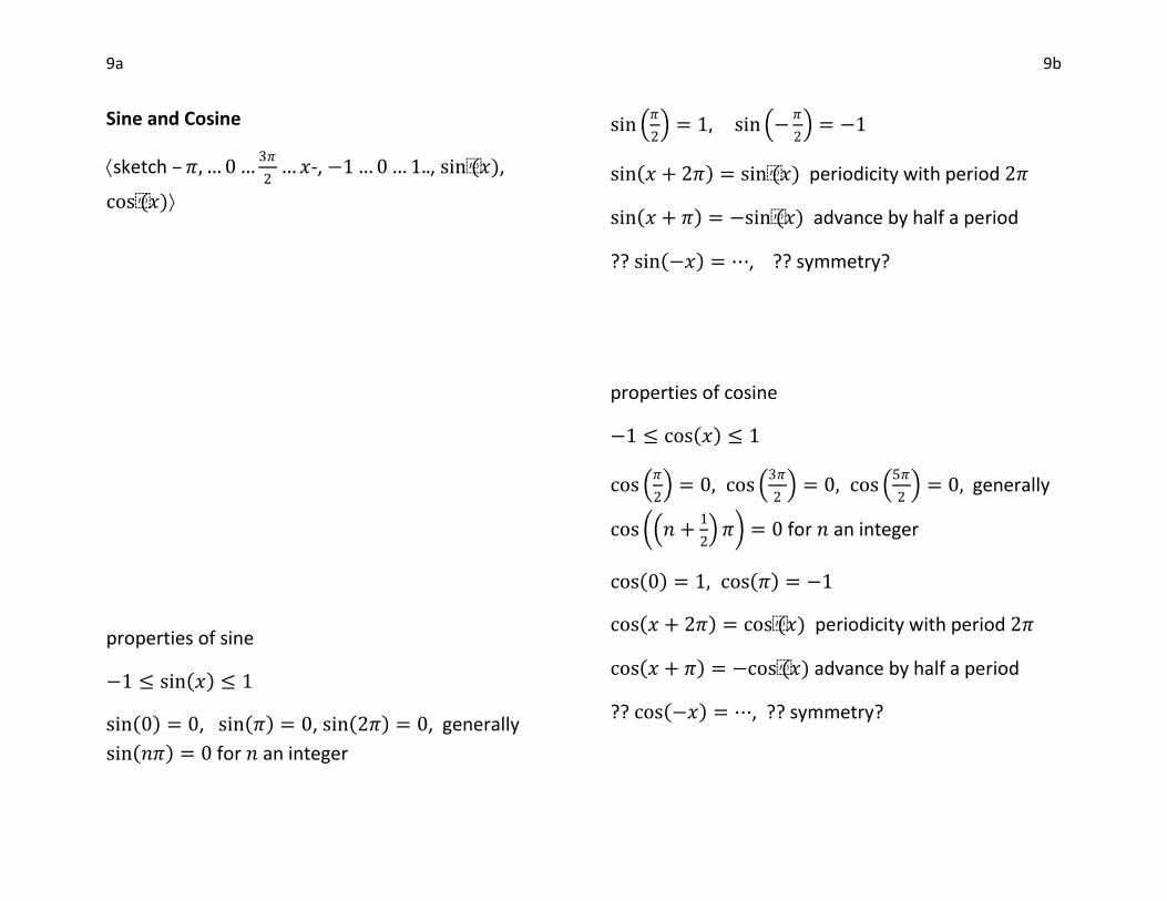
Sine and Cosine

sketch – 𝜋, … 0 …3𝜋

2…𝑥-, −1 … 0 … 1.., sin(𝑥),

cos(𝑥)

properties of sine

−1 ≤ sin 𝑥 ≤ 1

sin 0 = 0, sin 𝜋 = 0, sin 2𝜋 = 0, generally

sin 𝑛𝜋 = 0 for 𝑛 an integer

sin 𝜋

2 = 1, sin −

𝜋

2 = −1

sin 𝑥 + 2𝜋 = sin(𝑥) periodicity with period 2𝜋

sin 𝑥 + 𝜋 = −sin(𝑥) advance by half a period

?? sin −𝑥 = ⋯, ?? symmetry?

properties of cosine

−1 ≤ cos 𝑥 ≤ 1

cos 𝜋

2 = 0, cos

3𝜋

2 = 0, cos

5𝜋

2 = 0, generally

cos 𝑛 +1

2 𝜋 = 0 for 𝑛 an integer

cos 0 = 1, cos 𝜋 = −1

cos 𝑥 + 2𝜋 = cos(𝑥) periodicity with period 2𝜋

cos 𝑥 + 𝜋 = −cos(𝑥) advance by half a period

?? cos −𝑥 = ⋯, ?? symmetry?

10a 10b

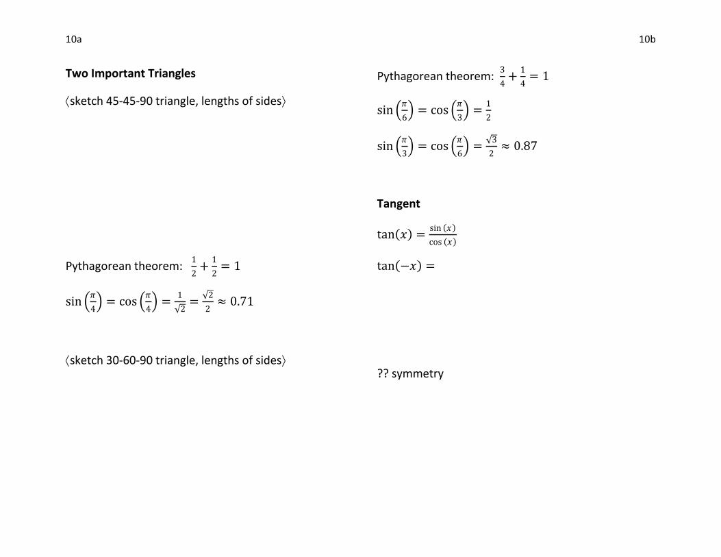
Two Important Triangles

sketch 45-45-90 triangle, lengths of sides

Pythagorean theorem: 1

2+

1

2= 1

sin 𝜋

4 = cos

𝜋

4 =

1

2=

2

2≈ 0.71

sketch 30-60-90 triangle, lengths of sides

Pythagorean theorem: 3

4+

1

4= 1

sin 𝜋

6 = cos

𝜋

3 =

1

2

sin 𝜋

3 = cos

𝜋

6 =

3

2≈ 0.87

Tangent

tan 𝑥 =sin 𝑥

cos 𝑥

tan −𝑥 =

?? symmetry

11a 11b

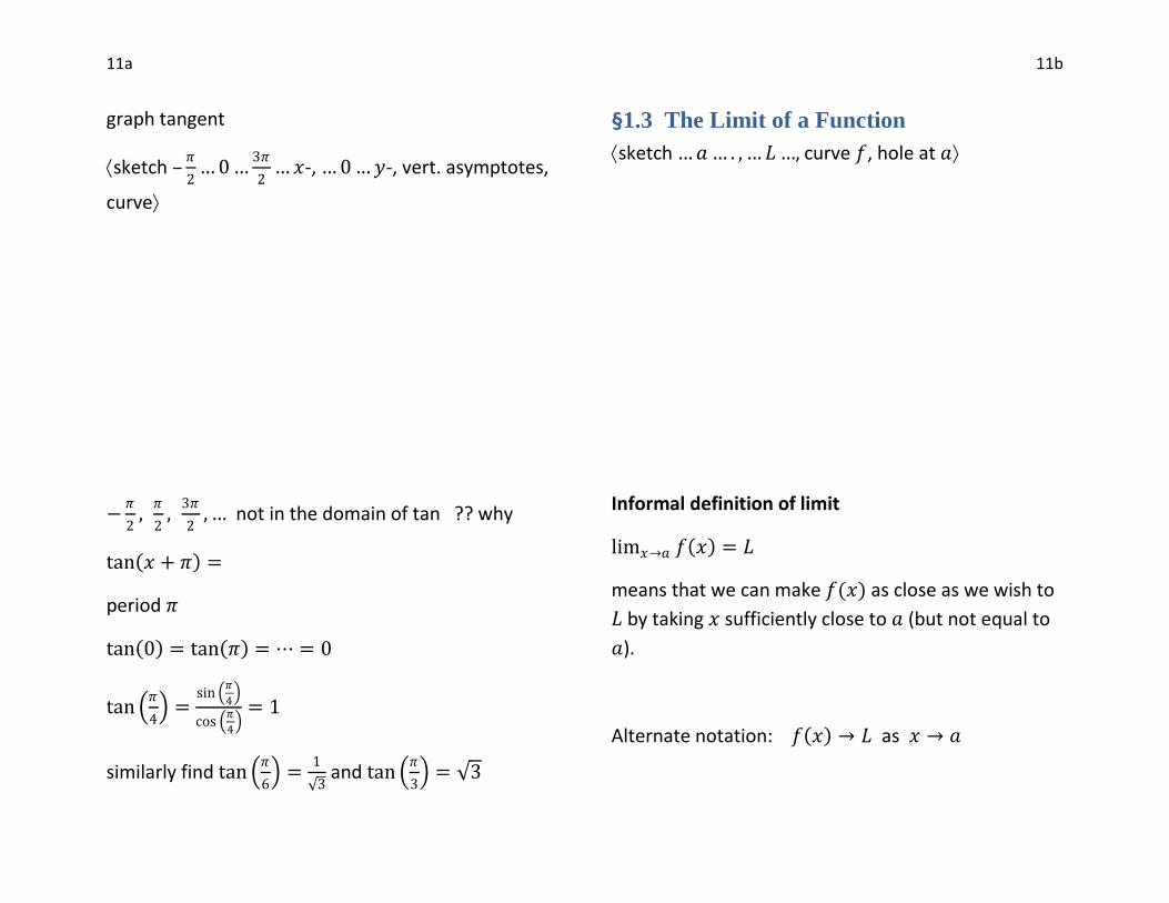
graph tangent

sketch –𝜋

2… 0 …

3𝜋

2…𝑥-, … 0 …𝑦-, vert. asymptotes,

curve

−𝜋

2,

𝜋

2,

3𝜋

2, … not in the domain of tan ?? why

tan 𝑥 + 𝜋 =

period 𝜋

tan 0 = tan 𝜋 = ⋯ = 0

tan 𝜋

4 =

sin 𝜋

4

cos 𝜋

4

= 1

similarly find tan 𝜋

6 =

1

3 and tan

𝜋

3 = 3

§1.3 The Limit of a Function

sketch …𝑎… . , …𝐿…, curve 𝑓, hole at 𝑎

Informal definition of limit

lim𝑥→𝑎 𝑓 𝑥 = 𝐿

means that we can make 𝑓(𝑥) as close as we wish to

𝐿 by taking 𝑥 sufficiently close to 𝑎 (but not equal to

𝑎).

Alternate notation: 𝑓 𝑥 → 𝐿 as 𝑥 → 𝑎

12a 12b

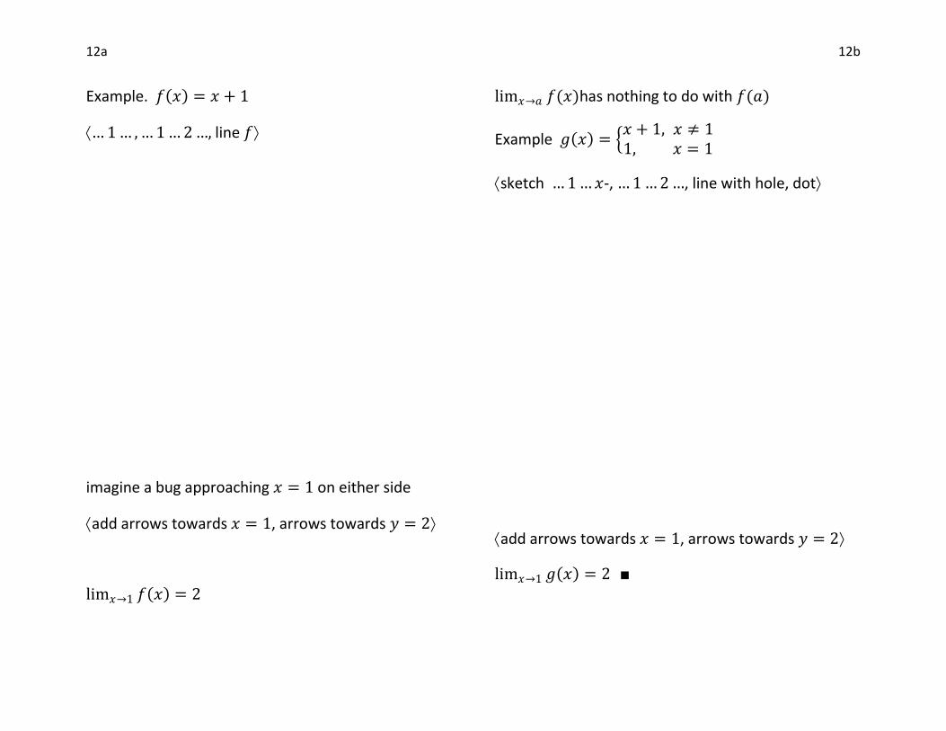
Example. 𝑓 𝑥 = 𝑥 + 1

… 1 … , … 1 … 2 …, line 𝑓

imagine a bug approaching 𝑥 = 1 on either side

add arrows towards 𝑥 = 1, arrows towards 𝑦 = 2

lim𝑥→1 𝑓 𝑥 = 2

lim𝑥→𝑎 𝑓(𝑥)has nothing to do with 𝑓(𝑎)

Example 𝑔 𝑥 = 𝑥 + 1, 𝑥 ≠ 11, 𝑥 = 1

sketch … 1 …𝑥-, … 1 … 2 …, line with hole, dot

add arrows towards 𝑥 = 1, arrows towards 𝑦 = 2

lim𝑥→1 𝑔 𝑥 = 2 ■

13a 13b

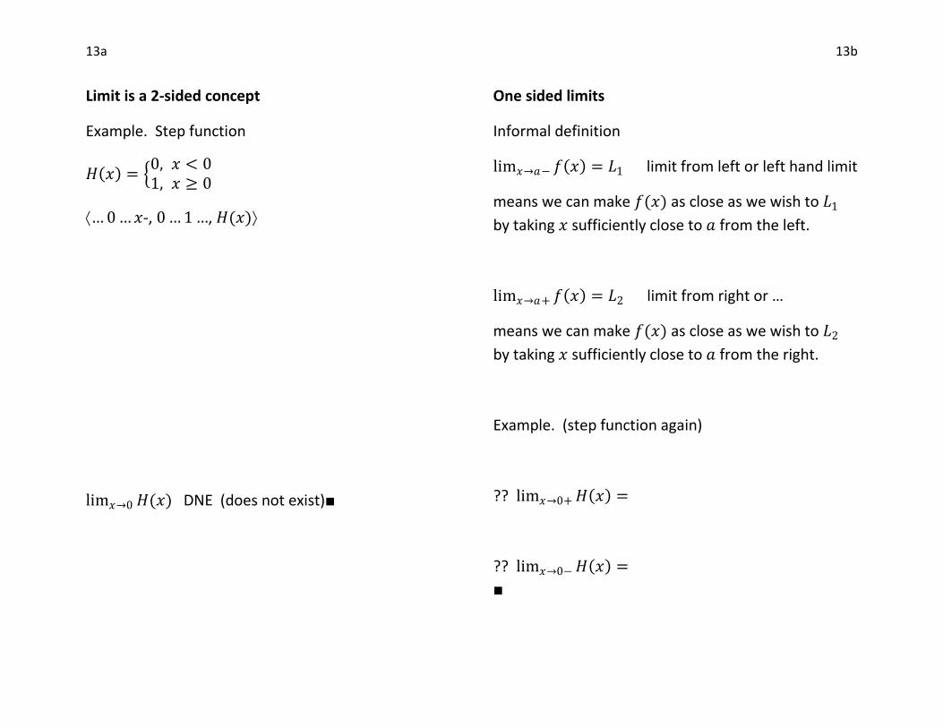
Limit is a 2-sided concept

Example. Step function

𝐻 𝑥 = 0, 𝑥 < 01, 𝑥 ≥ 0

… 0 …𝑥-, 0 … 1 …, 𝐻(𝑥)

lim𝑥→0 𝐻(𝑥) DNE (does not exist)■

One sided limits

Informal definition

lim𝑥→𝑎− 𝑓 𝑥 = 𝐿1 limit from left or left hand limit

means we can make 𝑓(𝑥) as close as we wish to 𝐿1

by taking 𝑥 sufficiently close to 𝑎 from the left.

lim𝑥→𝑎+ 𝑓 𝑥 = 𝐿2 limit from right or …

means we can make 𝑓(𝑥) as close as we wish to 𝐿2

by taking 𝑥 sufficiently close to 𝑎 from the right.

Example. (step function again)

?? lim𝑥→0+ 𝐻 𝑥 =

?? lim𝑥→0− 𝐻 𝑥 =

■

14a 14b

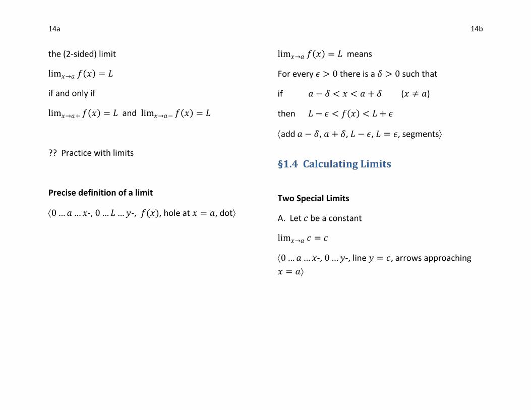
the (2-sided) limit

lim𝑥→𝑎 𝑓 𝑥 = 𝐿

if and only if

lim𝑥→𝑎+ 𝑓 𝑥 = 𝐿 and lim𝑥→𝑎− 𝑓 𝑥 = 𝐿

?? Practice with limits

Precise definition of a limit

0 …𝑎…𝑥-, 0 …𝐿…𝑦-, 𝑓(𝑥), hole at 𝑥 = 𝑎, dot

lim𝑥→𝑎 𝑓 𝑥 = 𝐿 means

For every 𝜖 > 0 there is a 𝛿 > 0 such that

if 𝑎 − 𝛿 < 𝑥 < 𝑎 + 𝛿 (𝑥 ≠ 𝑎)

then 𝐿 − 𝜖 < 𝑓 𝑥 < 𝐿 + 𝜖

add 𝑎 − 𝛿, 𝑎 + 𝛿, 𝐿 − 𝜖, 𝐿 = 𝜖, segments

§1.4 Calculating Limits

Two Special Limits

A. Let 𝑐 be a constant

lim𝑥→𝑎 𝑐 = 𝑐

0 …𝑎…𝑥-, 0 …𝑦-, line 𝑦 = 𝑐, arrows approaching

𝑥 = 𝑎

15a 15b

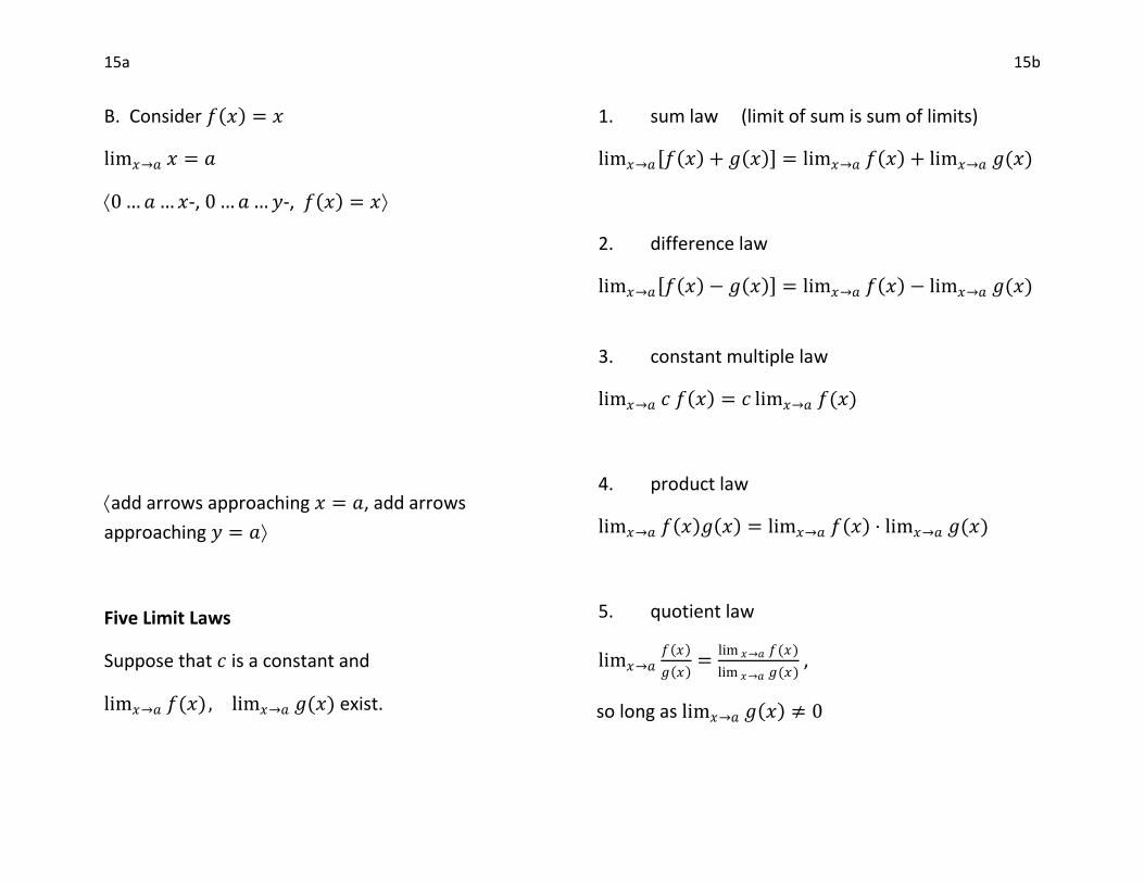
B. Consider 𝑓 𝑥 = 𝑥

lim𝑥→𝑎 𝑥 = 𝑎

0 …𝑎…𝑥-, 0 …𝑎…𝑦-, 𝑓 𝑥 = 𝑥

add arrows approaching 𝑥 = 𝑎, add arrows

approaching 𝑦 = 𝑎

Five Limit Laws

Suppose that 𝑐 is a constant and

lim𝑥→𝑎 𝑓(𝑥), lim𝑥→𝑎 𝑔(𝑥) exist.

1. sum law (limit of sum is sum of limits)

lim𝑥→𝑎 𝑓 𝑥 + 𝑔 𝑥 = lim𝑥→𝑎 𝑓 𝑥 + lim𝑥→𝑎 𝑔(𝑥)

2. difference law

lim𝑥→𝑎 𝑓 𝑥 − 𝑔 𝑥 = lim𝑥→𝑎 𝑓 𝑥 − lim𝑥→𝑎 𝑔(𝑥)

3. constant multiple law

lim𝑥→𝑎 𝑐 𝑓 𝑥 = 𝑐 lim𝑥→𝑎 𝑓(𝑥)

4. product law

lim𝑥→𝑎 𝑓 𝑥 𝑔 𝑥 = lim𝑥→𝑎 𝑓 𝑥 ⋅ lim𝑥→𝑎 𝑔(𝑥)

5. quotient law

lim𝑥→𝑎𝑓 𝑥

𝑔 𝑥 =

lim 𝑥→𝑎 𝑓(𝑥)

lim 𝑥→𝑎 𝑔(𝑥) ,

so long as lim𝑥→𝑎 𝑔 𝑥 ≠ 0

16a 16b

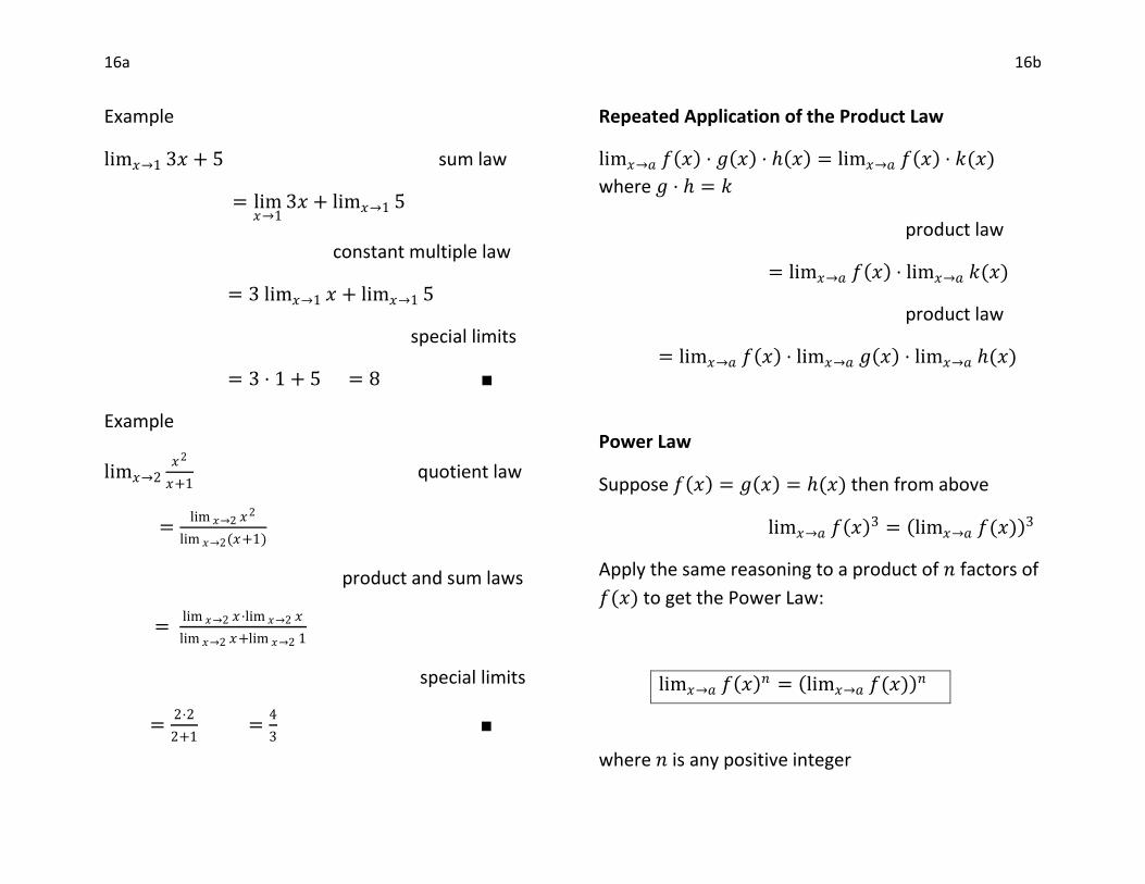
Example

lim𝑥→1 3𝑥 + 5 sum law

= lim𝑥→1

3𝑥 + lim𝑥→1 5

constant multiple law

= 3 lim𝑥→1 𝑥 + lim𝑥→1 5

special limits

= 3 ⋅ 1 + 5 = 8 ■

Example

lim𝑥→2𝑥2

𝑥+1 quotient law

=lim 𝑥→2 𝑥2

lim 𝑥→2(𝑥+1)

product and sum laws

= lim 𝑥→2 𝑥⋅lim 𝑥→2 𝑥

lim 𝑥→2 𝑥+lim 𝑥→2 1

special limits

=2⋅2

2+1 =

4

3 ■

Repeated Application of the Product Law

lim𝑥→𝑎 𝑓 𝑥 ⋅ 𝑔 𝑥 ⋅ 𝑕 𝑥 = lim𝑥→𝑎 𝑓 𝑥 ⋅ 𝑘(𝑥)

where 𝑔 ⋅ 𝑕 = 𝑘

product law

= lim𝑥→𝑎 𝑓 𝑥 ⋅ lim𝑥→𝑎 𝑘(𝑥)

product law

= lim𝑥→𝑎 𝑓 𝑥 ⋅ lim𝑥→𝑎 𝑔 𝑥 ⋅ lim𝑥→𝑎 𝑕(𝑥)

Power Law

Suppose 𝑓 𝑥 = 𝑔 𝑥 = 𝑕(𝑥) then from above

lim𝑥→𝑎 𝑓 𝑥 3 = lim𝑥→𝑎 𝑓(𝑥) 3

Apply the same reasoning to a product of 𝑛 factors of

𝑓(𝑥) to get the Power Law:

lim𝑥→𝑎 𝑓 𝑥 𝑛 = lim𝑥→𝑎 𝑓(𝑥) 𝑛

where 𝑛 is any positive integer

17a 17b

Example. Cubic Polynomial.

lim𝑥→2 𝑥3 − 4𝑥 difference law

= lim𝑥→2

𝑥3 − lim𝑥→2

4𝑥

power, constant multiple laws

= lim𝑥→2 𝑥 3 = 4 lim𝑥→2 𝑥

special limits

= 23 − 4 ⋅ 2 = 0 ■

Recall polynomials of degree 𝑛. Their general form is

𝑃 𝑥 = 𝑐𝑛𝑥𝑛 + 𝑐𝑛−1𝑥

𝑛−1 + ⋯ + 𝑐1𝑥 + 𝑐0

where 𝑐𝑛 , 𝑐𝑛−1, … , 𝑐1, 𝑐0 are constants.

By reasoning similar to the cubic polynomial example

lim𝑥→𝑎 𝑃 𝑥 sum law, const. multiple law

= 𝑐𝑛 lim𝑥→𝑎 𝑥𝑛 + ⋯ + 𝑐1 lim𝑥→𝑎 𝑥 + lim𝑥→𝑎 𝑐0

power law, special limit

= 𝑐𝑛𝑎𝑛 + ⋯𝑐1𝑎 + 𝑐0

= 𝑃(𝑎)

we have discovered the following

Direct Substitution Property for polynomials

If 𝑃(𝑥) is any polynomial and 𝑎 is a real number then

lim𝑥→𝑎 𝑃 𝑥 = 𝑃(𝑎).

This is much easier to apply than the limit laws!

Recall that a rational function is a ratio of two

polynomials.

𝑓 𝑥 =𝑃 𝑥

𝑄 𝑥 , where 𝑃 and 𝑄 are polynomials

Let 𝑓(𝑥) be any rational function

lim𝑥→𝑎 𝑓 𝑥 =lim 𝑥→𝑎 𝑃(𝑥)

lim 𝑥→𝑎 𝑄(𝑥) quotient law

=𝑃(𝑎)

𝑄(𝑎) direct subst. for polys

so long as 𝑄 𝑎 ≠ 0.

we now have a …

18a 18b

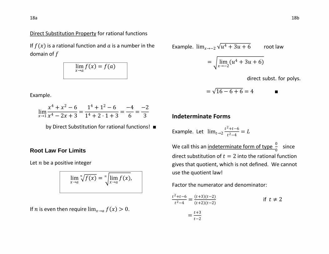
Direct Substitution Property for rational functions

If 𝑓(𝑥) is a rational function and 𝑎 is a number in the

domain of 𝑓

lim𝑥→𝑎

𝑓 𝑥 = 𝑓(𝑎)

Example.

lim𝑥→1

𝑥4 + 𝑥2 − 6

𝑥4 − 2𝑥 + 3=

14 + 12 − 6

14 + 2 ⋅ 1 + 3=

−4

6=

−2

3

by Direct Substitution for rational functions! ■

Root Law For Limits

Let 𝑛 be a positive integer

lim𝑥→𝑎

𝑓(𝑥)𝑛

= lim𝑥→𝑎

𝑓(𝑥)𝑛 ,

If 𝑛 is even then require lim𝑥→𝑎 𝑓 𝑥 > 0.

Example. lim𝑥→−2 𝑢4 + 3𝑢 + 6 root law

= lim𝑥→−2

(𝑢4 + 3𝑢 + 6)

direct subst. for polys.

= 16 − 6 + 6 = 4 ■

Indeterminate Forms

Example. Let lim𝑡→2𝑡2+𝑡−6

𝑡2−4= 𝐿

We call this an indeterminate form of type 0

0 since

direct substitution of 𝑡 = 2 into the rational function

gives that quotient, which is not defined. We cannot

use the quotient law!

Factor the numerator and denominator:

𝑡2+𝑡−6

𝑡2−4=

𝑡+3 (𝑡−2)

𝑡+2 (𝑡−2) if 𝑡 ≠ 2

=𝑡+3

𝑡−2

19a 19b

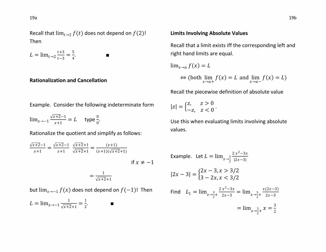
Recall that lim𝑡→2 𝑓(𝑡) does not depend on 𝑓(2)!

Then

𝐿 = lim𝑡→2𝑡+3

𝑡−3=

5

4. ■

Rationalization and Cancellation

Example. Consider the following indeterminate form

lim𝑥→−1 𝑥+2−1

𝑥+1= 𝐿 type

0

0.

Rationalize the quotient and simplify as follows:

𝑥+2−1

𝑥+1=

𝑥+2−1

𝑥+1 𝑥+2+1

𝑥+2+1=

(𝑥+1)

𝑥+1 ( 𝑥+2+1)

if 𝑥 ≠ −1

=1

𝑥+2+1

but lim𝑥→−1 𝑓(𝑥) does not depend on 𝑓(−1)! Then

𝐿 = lim𝑥→−11

𝑥+2+1=

1

2. ■

Limits Involving Absolute Values

Recall that a limit exists iff the corresponding left and

right hand limits are equal.

lim𝑥→𝑎 𝑓 𝑥 = 𝐿

⇔ (both lim𝑥→𝑎+

𝑓 𝑥 = 𝐿 and lim𝑥→𝑎−

𝑓 𝑥 = 𝐿)

Recall the piecewise definition of absolute value

𝑧 = 𝑧, 𝑧 > 0−𝑧, 𝑧 < 0

.

Use this when evaluating limits involving absolute

values.

Example. Let 𝐿 = lim𝑥→

3

2

2 𝑥2−3𝑥

|2𝑥−3|

2𝑥 − 3 = 2𝑥 − 3, 𝑥 > 3/23 − 2𝑥, 𝑥 < 3/2

Find 𝐿1 = lim𝑥→

3

2+

2 𝑥2−3𝑥

2𝑥−3= lim

𝑥→3

2+

𝑥(2𝑥−3)

2𝑥−3

= lim𝑥→

3

2+𝑥 =

3

2

20a 20b

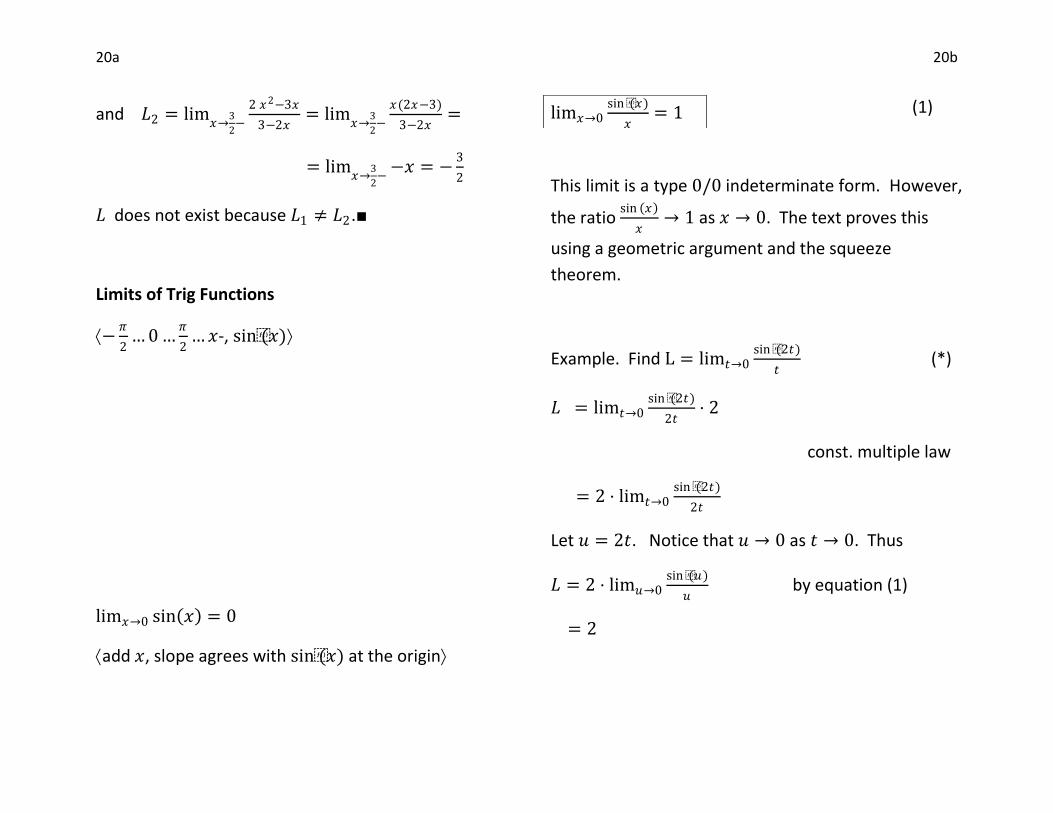
and 𝐿2 = lim𝑥→

3

2−

2 𝑥2−3𝑥

3−2𝑥= lim

𝑥→3

2−

𝑥(2𝑥−3)

3−2𝑥=

= lim𝑥→

3

2−−𝑥 = −

3

2

𝐿 does not exist because 𝐿1 ≠ 𝐿2.■

Limits of Trig Functions

−𝜋

2… 0 …

𝜋

2…𝑥-, sin(𝑥)

lim𝑥→0 sin 𝑥 = 0

add 𝑥, slope agrees with sin(𝑥) at the origin

(1)

This limit is a type 0/0 indeterminate form. However,

the ratio sin 𝑥

𝑥→ 1 as 𝑥 → 0. The text proves this

using a geometric argument and the squeeze

theorem.

Example. Find L = lim𝑡→0sin (2𝑡)

𝑡 (*)

𝐿 = lim𝑡→0sin (2𝑡)

2𝑡⋅ 2

const. multiple law

= 2 ⋅ lim𝑡→0sin (2𝑡)

2𝑡

Let 𝑢 = 2𝑡. Notice that 𝑢 → 0 as 𝑡 → 0. Thus

𝐿 = 2 ⋅ lim𝑢→0sin (𝑢)

𝑢 by equation (1)

= 2

lim𝑥→0sin (𝑥)

𝑥= 1

21a 21b

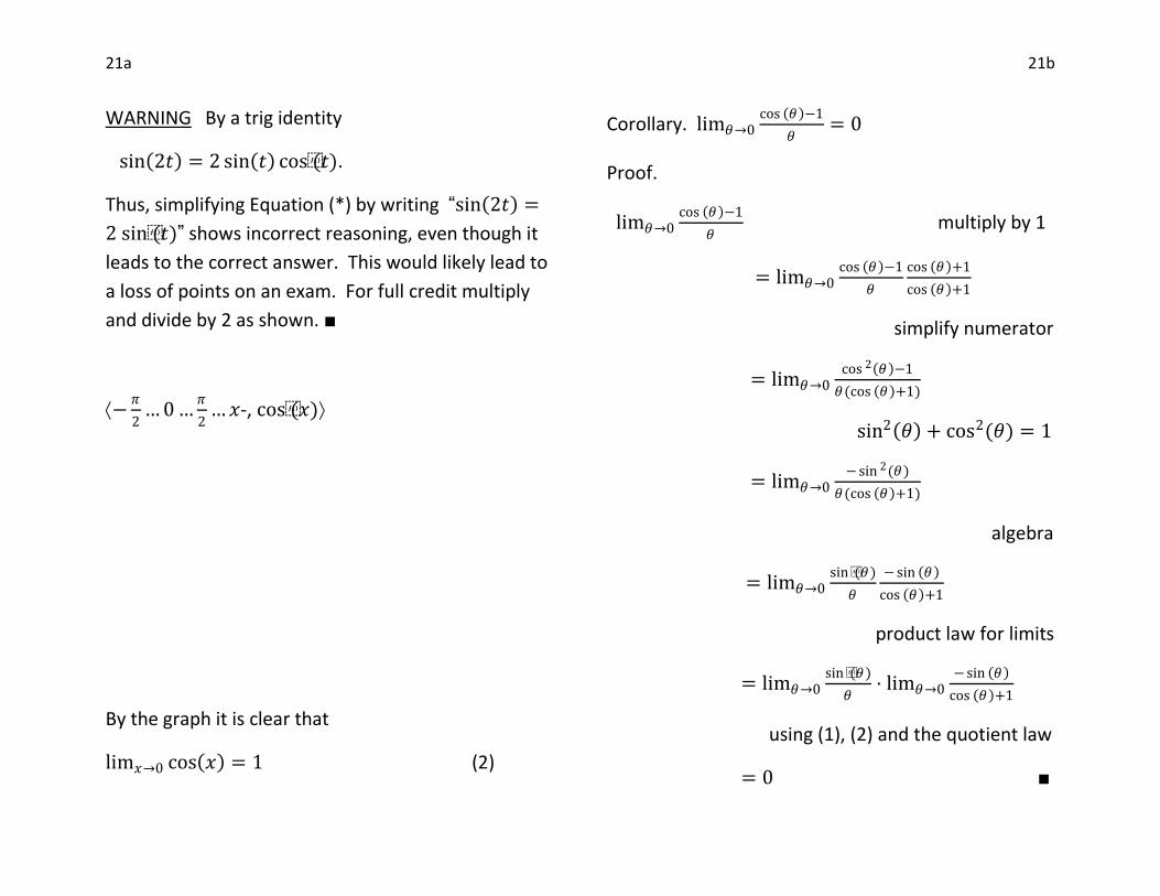
WARNING By a trig identity

sin 2𝑡 = 2 sin 𝑡 cos(𝑡).

Thus, simplifying Equation (*) by writing “sin 2𝑡 =

2 sin(𝑡)” shows incorrect reasoning, even though it

leads to the correct answer. This would likely lead to

a loss of points on an exam. For full credit multiply

and divide by 2 as shown. ■

−𝜋

2… 0 …

𝜋

2…𝑥-, cos(𝑥)

By the graph it is clear that

lim𝑥→0 cos 𝑥 = 1 (2)

Corollary. lim𝜃→0cos 𝜃 −1

𝜃= 0

Proof.

lim𝜃→0cos 𝜃 −1

𝜃 multiply by 1

= lim𝜃→0cos 𝜃 −1

𝜃

cos 𝜃 +1

cos 𝜃 +1

simplify numerator

= lim𝜃→0cos 2 𝜃 −1

𝜃(cos 𝜃 +1)

sin2 𝜃 + cos2(𝜃) = 1

= lim𝜃→0− sin 2(𝜃)

𝜃(cos 𝜃 +1)

algebra

= lim𝜃→0sin (𝜃)

𝜃

− sin 𝜃

cos 𝜃 +1

product law for limits

= lim𝜃→0sin (𝜃)

𝜃⋅ lim𝜃→0

− sin 𝜃

cos 𝜃 +1

using (1), (2) and the quotient law

= 0 ■

22a 22b

One further example.

?? Find L = lim𝑥→0tan (2𝑥)

𝑥.

■

§1.5 Continuity

Informal definition A function is continuous is it can

be drawn without removing pencil from the paper.

…𝑏…𝑎…𝑐…𝑥-. ,…𝑦-, 𝑓 continuous on 𝑏, 𝑐 ,

𝑔 with hole at 𝑎

𝑓 is continuous on (𝑏, 𝑐)

𝑔 is discontinuous at 𝑎.

common abbreviations: cts = continuous and dcts =

discontinuous.

23a 23b

Formal definition. A function 𝑓 is continuous at a

number 𝑎 if

lim𝑥→𝑎

𝑓 𝑥 = 𝑓(𝑎)

if not, 𝑓 is discontinuous at 𝑎.

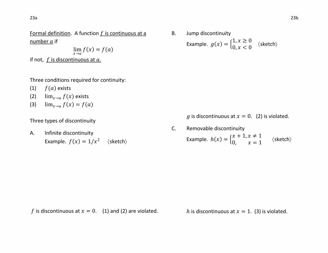
Three conditions required for continuity:

(1) 𝑓(𝑎) exists

(2) lim𝑥→𝑎 𝑓(𝑥) exists

(3) lim𝑥→𝑎 𝑓 𝑥 = 𝑓(𝑎)

Three types of discontinuity

A. Infinite discontinuity

Example. 𝑓 𝑥 = 1/𝑥2 sketch

𝑓 is discontinuous at 𝑥 = 0. (1) and (2) are violated.

B. Jump discontinuity

Example. 𝑔 𝑥 = 1, 𝑥 ≥ 00, 𝑥 < 0

sketch

𝑔 is discontinuous at 𝑥 = 0. (2) is violated.

C. Removable discontinuity

Example. 𝑕 𝑥 = 𝑥 + 1, 𝑥 ≠ 10, 𝑥 = 1

sketch

𝑕 is discontinuous at 𝑥 = 1. (3) is violated.

24a 24b

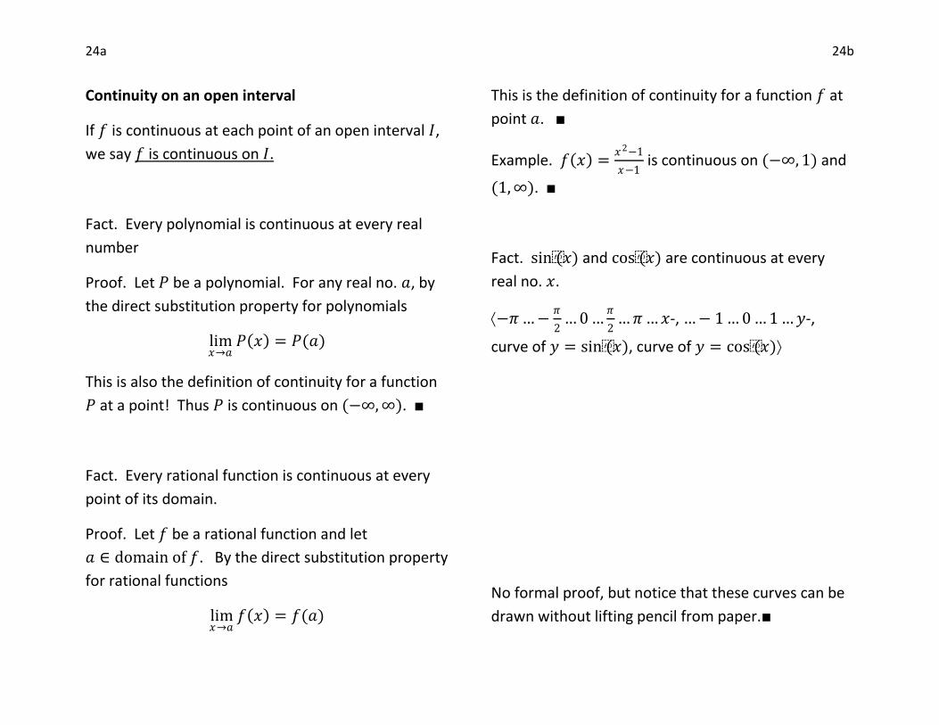
Continuity on an open interval

If 𝑓 is continuous at each point of an open interval 𝐼,

we say 𝑓 is continuous on 𝐼.

Fact. Every polynomial is continuous at every real

number

Proof. Let 𝑃 be a polynomial. For any real no. 𝑎, by

the direct substitution property for polynomials

lim𝑥→𝑎

𝑃 𝑥 = 𝑃(𝑎)

This is also the definition of continuity for a function

𝑃 at a point! Thus 𝑃 is continuous on (−∞, ∞). ■

Fact. Every rational function is continuous at every

point of its domain.

Proof. Let 𝑓 be a rational function and let

𝑎 ∈ domain of 𝑓. By the direct substitution property

for rational functions

lim𝑥→𝑎

𝑓 𝑥 = 𝑓(𝑎)

This is the definition of continuity for a function 𝑓 at

point 𝑎. ■

Example. 𝑓 𝑥 =𝑥2−1

𝑥−1 is continuous on (−∞, 1) and

(1,∞). ■

Fact. sin(𝑥) and cos(𝑥) are continuous at every

real no. 𝑥.

−𝜋…−𝜋

2… 0 …

𝜋

2…𝜋…𝑥-, …− 1 … 0 … 1 …𝑦-,

curve of 𝑦 = sin(𝑥), curve of 𝑦 = cos(𝑥)

No formal proof, but notice that these curves can be

drawn without lifting pencil from paper.■

25a 25b

Fact. 𝑦 = tan(𝑥) is continuous at every 𝑥 except

values 𝑥 =𝜋

2+ 𝑛𝜋, where 𝑛 is an integer.

Proof.

lim𝑥→𝑎 tan 𝑥 = lim𝑥→𝑎sin 𝑥

cos 𝑥 quotient law

=lim 𝑥→𝑎 sin 𝑥

lim 𝑥→𝑎 cos 𝑥 cty of sin & cos

= tan(𝑎)

unless cos 𝑎 = 0.

But from graph above, cos 𝑎 = 0 except at

𝑥 =𝜋

2+ 𝑛𝜋, where 𝑛 is an integer. ■

Theorem (Arithmetic combinations of continuous

functions)

If 𝑓 and 𝑔 are continuous at no. 𝑎 and 𝑐 is a constant,

then the following combinations are continuous at 𝑎.

1. 𝑓 + 𝑔 sum

2. 𝑓 − 𝑔 difference

3. 𝑐𝑓 constant multiple

4. 𝑓𝑔 product

5. 𝑓/𝑔 provided 𝑔 𝑎 ≠ 0 quotient

Proof. Each part follows from the corresponding limit

law. For example, consider (4)

lim𝑥→𝑎 𝑓 𝑥 ⋅ 𝑔 𝑥 product law for limits

= lim𝑥→𝑎 𝑓 𝑥 ⋅ lim𝑥→𝑎 𝑔(𝑥)

continuity of 𝑓 and 𝑔

= 𝑓 𝑎 ⋅ 𝑔(𝑎)

This is the definition of continuity of 𝑓 𝑥 ⋅ 𝑔(𝑥) ■

26a 26b

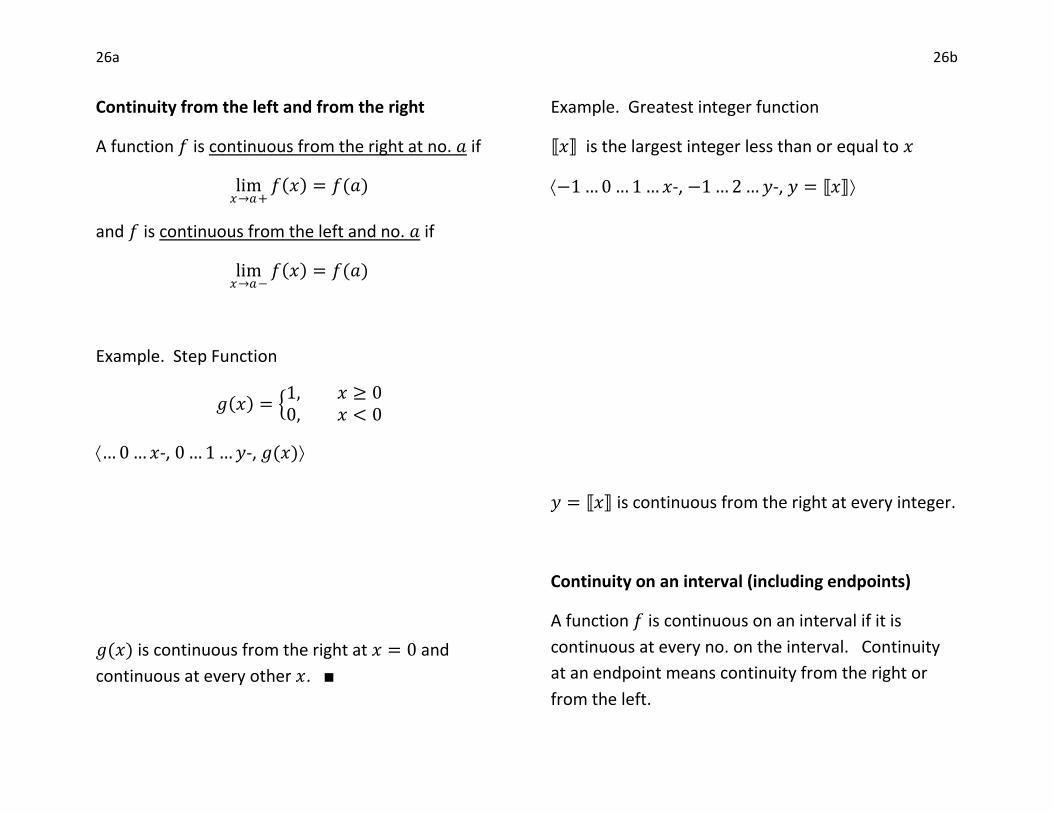
Continuity from the left and from the right

A function 𝑓 is continuous from the right at no. 𝑎 if

lim𝑥→𝑎+

𝑓 𝑥 = 𝑓(𝑎)

and 𝑓 is continuous from the left and no. 𝑎 if

lim𝑥→𝑎−

𝑓 𝑥 = 𝑓(𝑎)

Example. Step Function

𝑔 𝑥 = 1, 𝑥 ≥ 00, 𝑥 < 0

… 0 …𝑥-, 0 … 1 …𝑦-, 𝑔(𝑥)

𝑔(𝑥) is continuous from the right at 𝑥 = 0 and

continuous at every other 𝑥. ■

Example. Greatest integer function

𝑥 is the largest integer less than or equal to 𝑥

−1 … 0 … 1 …𝑥-, −1 … 2 …𝑦-, 𝑦 = 𝑥

𝑦 = 𝑥 is continuous from the right at every integer.

Continuity on an interval (including endpoints)

A function 𝑓 is continuous on an interval if it is

continuous at every no. on the interval. Continuity

at an endpoint means continuity from the right or

from the left.

27a 27b

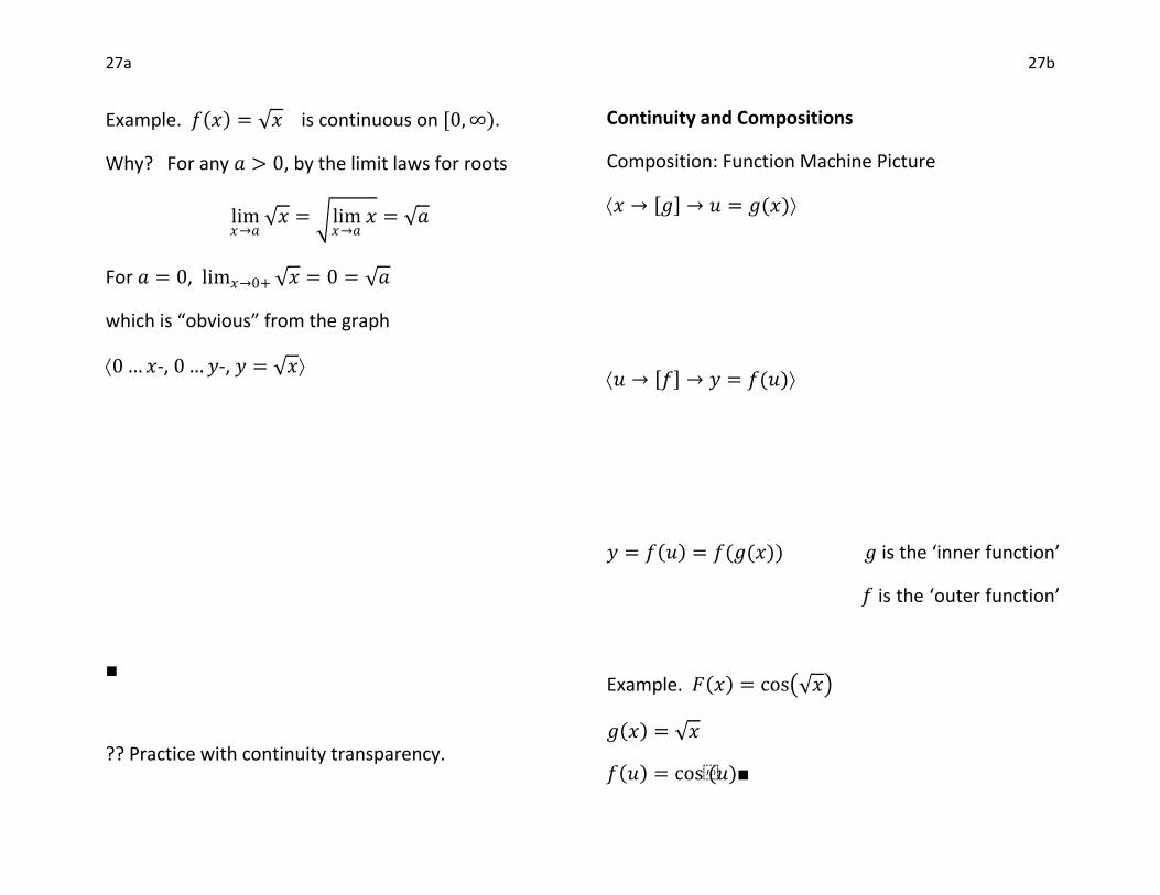
Example. 𝑓 𝑥 = 𝑥 is continuous on [0, ∞).

Why? For any 𝑎 > 0, by the limit laws for roots

lim𝑥→𝑎

𝑥 = lim𝑥→𝑎

𝑥 = 𝑎

For 𝑎 = 0, lim𝑥→0+ 𝑥 = 0 = 𝑎

which is “obvious” from the graph

0 …𝑥-, 0 …𝑦-, 𝑦 = 𝑥

■

?? Practice with continuity transparency.

Continuity and Compositions

Composition: Function Machine Picture

𝑥 → 𝑔 → 𝑢 = 𝑔(𝑥)

𝑢 → 𝑓 → 𝑦 = 𝑓(𝑢)

𝑦 = 𝑓 𝑢 = 𝑓(𝑔(𝑥)) 𝑔 is the ‘inner function’

𝑓 is the ‘outer function’

Example. 𝐹 𝑥 = cos 𝑥

𝑔 𝑥 = 𝑥

𝑓 𝑢 = cos(𝑢)■

28a 28b

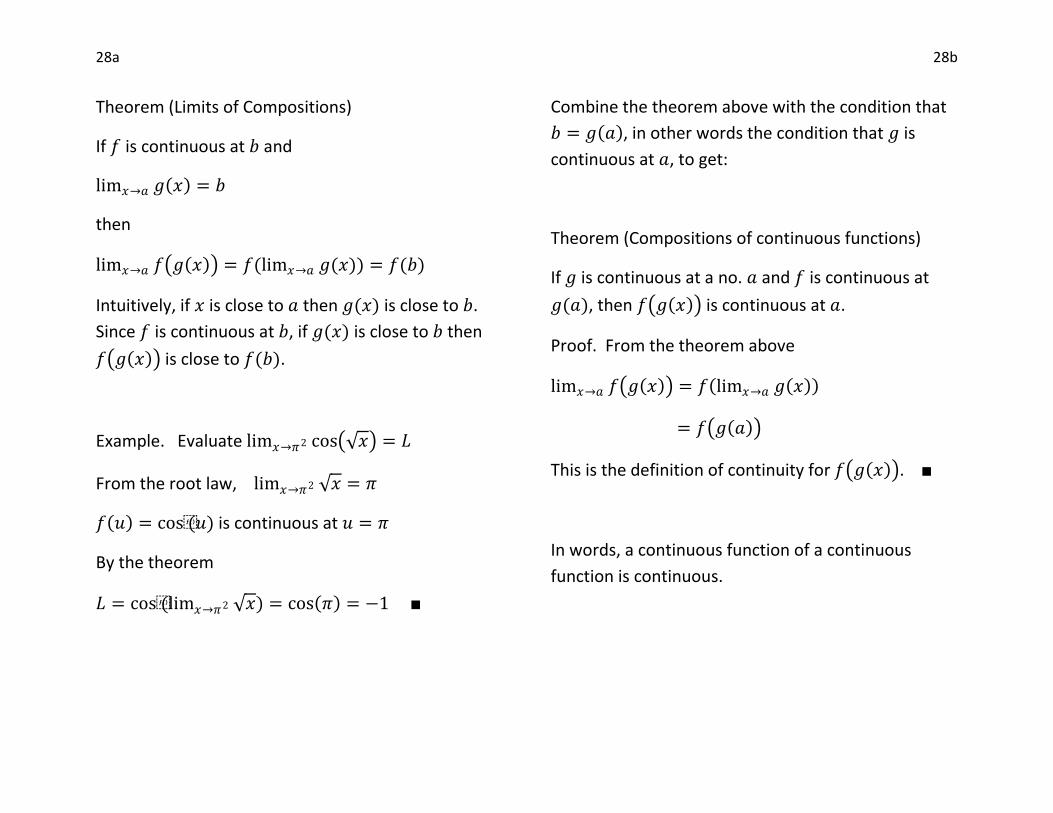
Theorem (Limits of Compositions)

If 𝑓 is continuous at 𝑏 and

lim𝑥→𝑎 𝑔 𝑥 = 𝑏

then

lim𝑥→𝑎 𝑓 𝑔 𝑥 = 𝑓(lim𝑥→𝑎 𝑔(𝑥)) = 𝑓(𝑏)

Intuitively, if 𝑥 is close to 𝑎 then 𝑔(𝑥) is close to 𝑏.

Since 𝑓 is continuous at 𝑏, if 𝑔(𝑥) is close to 𝑏 then

𝑓 𝑔 𝑥 is close to 𝑓(𝑏).

Example. Evaluate lim𝑥→𝜋2 cos 𝑥 = 𝐿

From the root law, lim𝑥→𝜋2 𝑥 = 𝜋

𝑓 𝑢 = cos(𝑢) is continuous at 𝑢 = 𝜋

By the theorem

𝐿 = cos(lim𝑥→𝜋2 𝑥) = cos 𝜋 = −1 ■

Combine the theorem above with the condition that

𝑏 = 𝑔 𝑎 , in other words the condition that 𝑔 is

continuous at 𝑎, to get:

Theorem (Compositions of continuous functions)

If 𝑔 is continuous at a no. 𝑎 and 𝑓 is continuous at

𝑔(𝑎), then 𝑓 𝑔 𝑥 is continuous at 𝑎.

Proof. From the theorem above

lim𝑥→𝑎 𝑓 𝑔 𝑥 = 𝑓 lim𝑥→𝑎 𝑔 𝑥

= 𝑓 𝑔 𝑎

This is the definition of continuity for 𝑓 𝑔 𝑥 . ■

In words, a continuous function of a continuous

function is continuous.

29a 29b

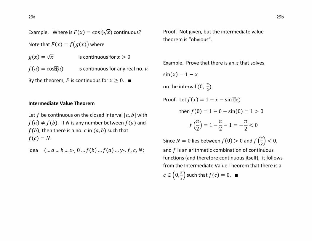
Example. Where is 𝐹 𝑥 = cos( 𝑥) continuous?

Note that 𝐹 𝑥 = 𝑓 𝑔 𝑥 where

𝑔 𝑥 = 𝑥 is continuous for 𝑥 > 0

𝑓 𝑢 = cos(𝑢) is continuous for any real no. 𝑢

By the theorem, 𝐹 is continuous for 𝑥 ≥ 0. ■

Intermediate Value Theorem

Let 𝑓 be continuous on the closed interval [𝑎, 𝑏] with

𝑓 𝑎 ≠ 𝑓(𝑏). If 𝑁 is any number between 𝑓(𝑎) and

𝑓(𝑏), then there is a no. 𝑐 in (𝑎, 𝑏) such that

𝑓 𝑐 = 𝑁.

Idea …𝑎…𝑏…𝑥-, 0 …𝑓 𝑏 …𝑓 𝑎 …𝑦-, 𝑓, 𝑐, 𝑁

Proof. Not given, but the intermediate value

theorem is “obvious”.

Example. Prove that there is an 𝑥 that solves

sin 𝑥 = 1 − 𝑥

on the interval (0,𝜋

2).

Proof. Let 𝑓 𝑥 = 1 − 𝑥 − sin(𝑥)

then 𝑓 0 = 1 − 0 − sin 0 = 1 > 0

𝑓 𝜋

2 = 1 −

𝜋

2− 1 = −

𝜋

2< 0

Since 𝑁 = 0 lies between 𝑓 0 > 0 and 𝑓 𝜋

2 < 0,

and 𝑓 is an arithmetic combination of continuous

functions (and therefore continuous itself), it follows

from the Intermediate Value Theorem that there is a

𝑐 ∈ 0,𝜋

2 such that 𝑓 𝑐 = 0. ■

30a 30b

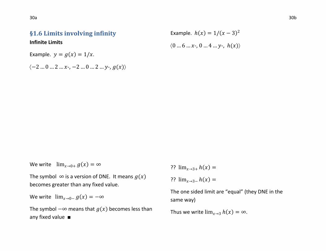
§1.6 Limits involving infinity

Infinite Limits

Example. 𝑦 = 𝑔 𝑥 = 1/𝑥.

−2 … 0 … 2 …𝑥-, −2 … 0 … 2 …𝑦-, 𝑔(𝑥)

We write lim𝑥→0+ 𝑔 𝑥 = ∞

The symbol ∞ is a version of DNE. It means 𝑔(𝑥)

becomes greater than any fixed value.

We write lim𝑥→0− 𝑔 𝑥 = −∞

The symbol −∞ means that 𝑔(𝑥) becomes less than

any fixed value ■

Example. 𝑕 𝑥 = 1/ 𝑥 − 3 2

0 … 6 …𝑥-, 0 … 4 …𝑦-, 𝑕(𝑥)

?? lim𝑥→3+ 𝑕 𝑥 =

?? lim𝑥→3− 𝑕 𝑥 =

The one sided limit are “equal” (they DNE in the

same way)

Thus we write lim𝑥→3 𝑕 𝑥 = ∞.

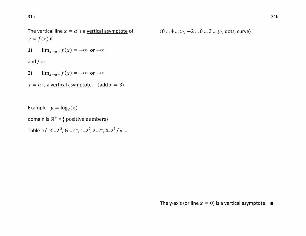
31a 31b

The vertical line 𝑥 = 𝑎 is a vertical asymptote of

𝑦 = 𝑓(𝑥) if

1) lim𝑥→𝑎+ 𝑓 𝑥 = +∞ or −∞

and / or

2) lim𝑥→𝑎− 𝑓 𝑥 = +∞ or −∞

𝑥 = 𝑎 is a vertical asymptote. add 𝑥 = 3

Example. 𝑦 = log2(𝑥)

domain is ℝ+ = { positive numbers}

Table x/ ¼ =2-2, ½ =2-1, 1=20, 2=21, 4=22 / y …

0 … 4 …𝑥-, −2 … 0 … 2 …𝑦-, dots, curve

The y-axis (or line 𝑥 = 0) is a vertical asymptote. ■

32a 32b

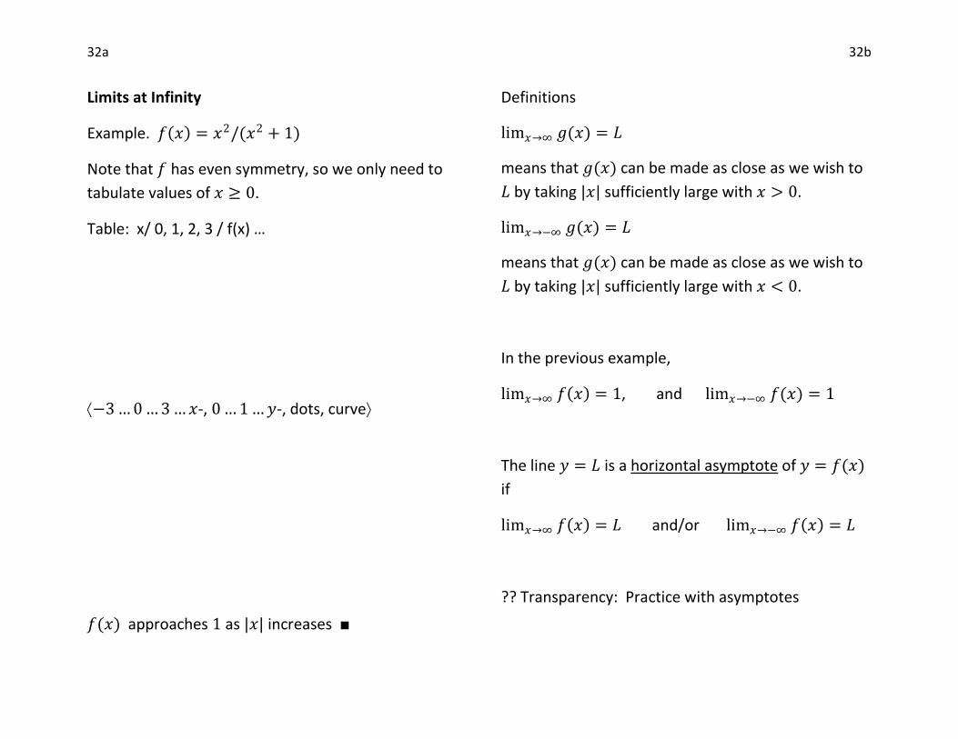
Limits at Infinity

Example. 𝑓 𝑥 = 𝑥2/(𝑥2 + 1)

Note that 𝑓 has even symmetry, so we only need to

tabulate values of 𝑥 ≥ 0.

Table: x/ 0, 1, 2, 3 / f(x) …

−3 … 0 … 3 …𝑥-, 0 … 1 …𝑦-, dots, curve

𝑓(𝑥) approaches 1 as |𝑥| increases ■

Definitions

lim𝑥→∞ 𝑔(𝑥) = 𝐿

means that 𝑔(𝑥) can be made as close as we wish to

𝐿 by taking |𝑥| sufficiently large with 𝑥 > 0.

lim𝑥→−∞ 𝑔(𝑥) = 𝐿

means that 𝑔(𝑥) can be made as close as we wish to

𝐿 by taking |𝑥| sufficiently large with 𝑥 < 0.

In the previous example,

lim𝑥→∞ 𝑓 𝑥 = 1, and lim𝑥→−∞ 𝑓(𝑥) = 1

The line 𝑦 = 𝐿 is a horizontal asymptote of 𝑦 = 𝑓(𝑥)

if

lim𝑥→∞ 𝑓 𝑥 = 𝐿 and/or lim𝑥→−∞ 𝑓 𝑥 = 𝐿

?? Transparency: Practice with asymptotes

33a 33b

Consider lim𝑥→∞ 1/𝑥

For 𝑥 > 10, 0 <1

𝑥<

1

10

For 𝑥 > 100, 0 <1

𝑥<

1

100

We can make 1/𝑥 as close as we wish to zero by

taking 𝑥 sufficiently large. Conclude

lim𝑥→∞1

𝑥= 0

Consider lim𝑥→−∞ 1/𝑥

For 𝑥 < −10, −1

10<

1

𝑥< 0

For 𝑥 < −100,−1

100<

1

𝑥< 0

We can make 1/𝑥 as close as we wish to zero by

taking |𝑥| sufficiently large with 𝑥 < 0. Conclude

lim𝑥→−∞1

𝑥= 0

Generalize

If 𝑟 is a positive real number

lim𝑥→∞1

𝑥𝑟= 0 Equation (1)

we won’t prove this

Examples. lim𝑥→∞1

𝑥2= 0

lim𝑥→∞1

𝑥= lim𝑥→∞

1

𝑥12

= 0 ■

Infinite Limit Laws

These are obtained from the limit laws we have

already seen by replacing 𝑎 with ±∞.

Suppose that 𝑐 is a constant and

lim𝑥→±∞ 𝑓(𝑥), lim𝑥→±∞ 𝑔(𝑥)exist.

1. sum law (limit of sum is sum of limits)

lim𝑥→±∞

𝑓 𝑥 + 𝑔 𝑥 = lim𝑥→±∞

𝑓 𝑥 + lim𝑥→±∞

𝑔(𝑥)

34a 34b

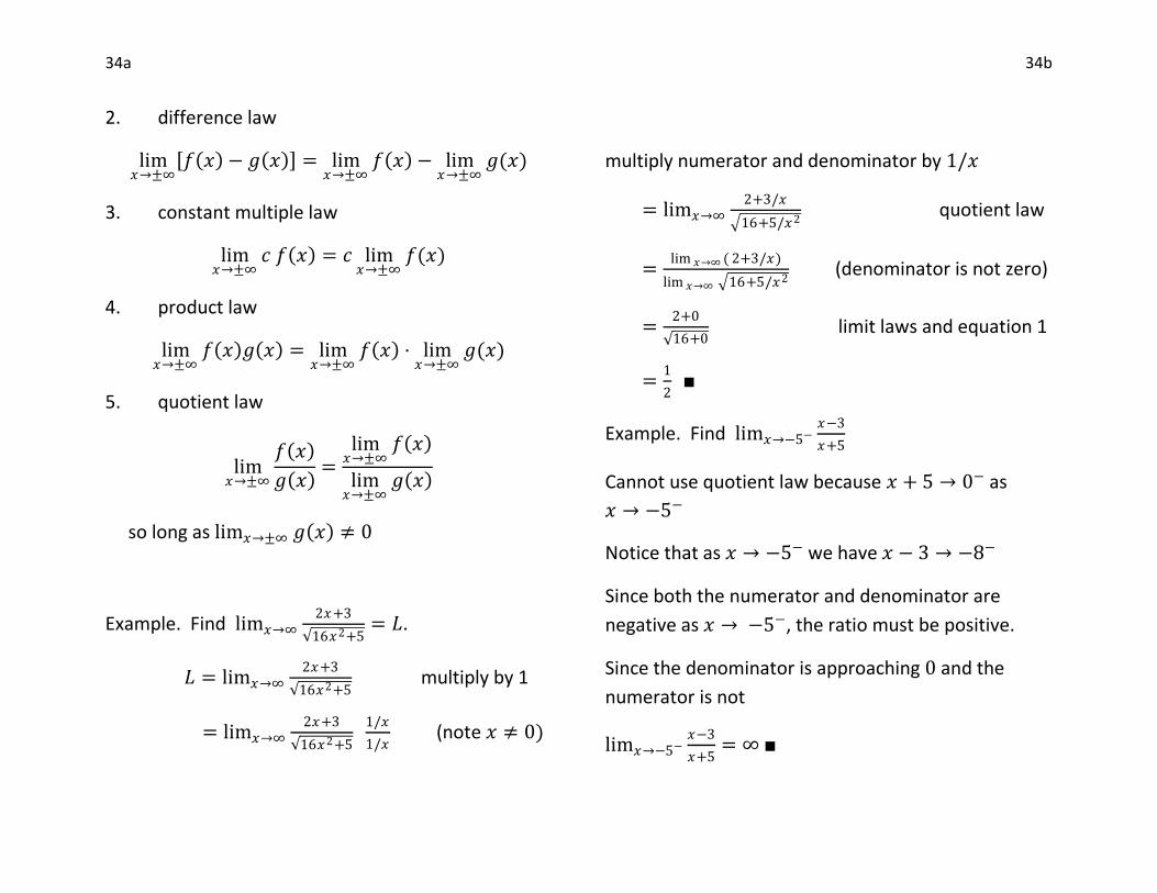
2. difference law

lim𝑥→±∞

𝑓 𝑥 − 𝑔 𝑥 = lim𝑥→±∞

𝑓 𝑥 − lim𝑥→±∞

𝑔(𝑥)

3. constant multiple law

lim𝑥→±∞

𝑐 𝑓 𝑥 = 𝑐 lim𝑥→±∞

𝑓(𝑥)

4. product law

lim𝑥→±∞

𝑓 𝑥 𝑔 𝑥 = lim𝑥→±∞

𝑓 𝑥 ⋅ lim𝑥→±∞

𝑔(𝑥)

5. quotient law

lim𝑥→±∞

𝑓 𝑥

𝑔 𝑥 =

lim𝑥→±∞

𝑓 𝑥

lim𝑥→±∞

𝑔 𝑥

so long as lim𝑥→±∞ 𝑔 𝑥 ≠ 0

Example. Find lim𝑥→∞2𝑥+3

16𝑥2+5= 𝐿.

𝐿 = lim𝑥→∞2𝑥+3

16𝑥2+5 multiply by 1

= lim𝑥→∞2𝑥+3

16𝑥2+5

1/𝑥

1/𝑥 (note 𝑥 ≠ 0)

multiply numerator and denominator by 1/𝑥

= lim𝑥→∞2+3/𝑥

16+5/𝑥2 quotient law

=lim 𝑥→∞ ( 2+3/𝑥)

lim 𝑥→∞ 16+5/𝑥2 (denominator is not zero)

=2+0

16+0 limit laws and equation 1

=1

2 ■

Example. Find lim𝑥→−5−𝑥−3

𝑥+5

Cannot use quotient law because 𝑥 + 5 → 0− as

𝑥 → −5−

Notice that as 𝑥 → −5− we have 𝑥 − 3 → −8−

Since both the numerator and denominator are

negative as 𝑥 → −5−, the ratio must be positive.

Since the denominator is approaching 0 and the

numerator is not

lim𝑥→−5−𝑥−3

𝑥+5= ∞ ■