Embed Size (px)
Citation preview

Business Mathematics
Tomastik/Epstein
0.0 CONTENTS 1
Contents
1 Systems of Linear Equations and Models 2
1.1 Mathematical Models . . . . . . . . . . . . . . . . . . . . . . 3
1.2 Systems of Linear Equations . . . . . . . . . . . . . . . . . . . 19
1.3 Gauss Elimination for Systems of Linear Equations . . . . . . . 28
1.4 Systems of Linear Equations With Non-Unique Solutions . . . 45
1.5 Method of Least Squares . . . . . . . . . . . . . . . . . . . . . 61
Review . . . . . . . . . . . . . . . . . . . . . . . . . . . . . . 71
2 Matrices 76
2.1 Introduction to Matrices . . . . . . . . . . . . . . . . . . . . . 77
2.2 Matrix Multiplication . . . . . . . . . . . . . . . . . . . . . . . 87
2.3 Inverse of a Square Matrix . . . . . . . . . . . . . . . . . . . . 103
2.4 Additional Matrix Applications . . . . . . . . . . . . . . . . . . 116
Review . . . . . . . . . . . . . . . . . . . . . . . . . . . . . . 128
3 Linear Programming 132
3.1 Linear Programming Problems . . . . . . . . . . . . . . . . . . 133
3.2 Graphing Linear Inequalities . . . . . . . . . . . . . . . . . . . 146
3.3 Graphical Solution of Linear Programming Problems . . . . . . 156
3.4 The Simplex Method . . . . . . . . . . . . . . . . . . . . . . . 167
3.5 Post-Optimal Analysis . . . . . . . . . . . . . . . . . . . . . . 192
Review . . . . . . . . . . . . . . . . . . . . . . . . . . . . . . 204
4 Probability 208
4.1 Sample Spaces and Events . . . . . . . . . . . . . . . . . . . . 208
4.2 Basics of Probability . . . . . . . . . . . . . . . . . . . . . . . 216
4.3 Rules for Probability . . . . . . . . . . . . . . . . . . . . . . . 223
4.4 Random Variables and Expected Value . . . . . . . . . . . . . 232
4.5 Conditional Probability . . . . . . . . . . . . . . . . . . . . . . 246
4.6 Bayes’ Theorem . . . . . . . . . . . . . . . . . . . . . . . . . . 258
Review . . . . . . . . . . . . . . . . . . . . . . . . . . . . . . 266
5 Functions and Models 271
5.1 Polynomials . . . . . . . . . . . . . . . . . . . . . . . . . . . 271
5.2 Power, Rational, and Piecewise Defined Functions . . . . . . . 288
5.3 Exponential Functions . . . . . . . . . . . . . . . . . . . . . . 297
5.4 Combinations of Functions . . . . . . . . . . . . . . . . . . . . 304
5.5 Inverse Functions and Logarithms . . . . . . . . . . . . . . . . 312
5.6 Review . . . . . . . . . . . . . . . . . . . . . . . . . . . . . . 322
6 Finance 331
6.1 Simple and Compound Interest . . . . . . . . . . . . . . . . . 331
6.2 Annuities and Sinking Funds . . . . . . . . . . . . . . . . . . . 340
6.3 Present Value of Annuities and Amortization . . . . . . . . . . 346
Review . . . . . . . . . . . . . . . . . . . . . . . . . . . . . . 354
2 Chapter 0 CONTENTS
T Technology 357
T.1 Systems of Linear Equations and Models . . . . . . . . . . . . 357
T.2 Matrices . . . . . . . . . . . . . . . . . . . . . . . . . . . . . . 365
T.3 Linear Programming . . . . . . . . . . . . . . . . . . . . . . . 368
T.4 Probability . . . . . . . . . . . . . . . . . . . . . . . . . . . . . 376
T.5 Functions and Modeling . . . . . . . . . . . . . . . . . . . . . 377
T.6 Finance . . . . . . . . . . . . . . . . . . . . . . . . . . . . . . 379
Answers to Selected Exercises 380
Bibliography 397
Index 403
CHAPTER 1Systems of Linear Equations and Models
CONNECTION
Demand for Televisions
As sleek flat-panel and high-definition television
sets became more affordable, sales soared during
the holidays. Sales of ultra-thin, wall-mountable
LCD TVs rose over 100% in 2005 to about 20
million sets while plasma-TV sales rose at a sim-
ilar pace, to about 5 million sets. Normally set
makers and retailers lower their prices after the
holidays, but since there was strong demand and
production shortages for these sets, prices were
kept high.Source: http://biz.yahoo.com
1.1 Mathematical Models 3
1.1 Mathematical Models
APPLICATION
Cost, Revenue, and Profit
Models
A firm has weekly fixed costs of $80,000 associated with the manufacture
of dresses that cost $25 per dress to produce. The firm sells all the dresses
it produces at $75 per dress. Find the cost, revenue, and profit equations
if x is the number of dresses produced per week. See Example 3 for the
answer.
We will first review some basic material on functions. An introduction to the
mathematical theory of the business firm with some necessary economics back-
ground is provided. We study mathematical business models of cost, revenue,
profit, and depreciation, and mathematical economic models of demand and sup-
ply.
✧ Functions
Mathematical modeling is an attempt to describe some part of the real world in
mathematical terms. Our models will be functions that show the relationship
between two or more variables. These variables will represent quantities that we
wish to understand or describe. Examples include the price of gasoline, the cost
of producing cereal, or the number of video games sold. The idea of representing
these quantities as variables in a function is central to our goal of creating models
to describe their behavior. We will begin by reviewing the concept of functions.
In short, we call any rule that assigns or corresponds to each element in one set
precisely one element in another set a function.
HISTORICAL NOTE
Augustin Cournot
(1801–1877)
The first significant work dealing
with the application of mathematics
to economics was Cournot’s
Researches into the Mathematical
Principles of the Theory of Wealth,
published in 1836. It was Cournot
who originated the supply and
demand curves that are discussed
in this section. Irving Fisher, a
prominent economics professor at
Yale University and one of the first
exponents of mathematical
economics in the United States,
wrote that Cournot’s book “seemed
a failure when first published. It
was far in advance of the times. Its
methods were too strange, its
reasoning too intricate for the
crude and confident notions of
political economy then current.”
For example, suppose you are going a steady speed of 40 miles per hour
in a car. In one hour you will travel 40 miles; in two hours you will travel 80
miles; and so on. The distance you travel depends on (corresponds to) the time.
Indeed, the equation relating the variables distance (d), velocity (v), and time (t),
is d = v ·t. In our example, we have a constant velocity of v= 40, so d = 40 ·t. We
can view this as a correspondence or rule: Given the time t in hours, the rule gives
a distance d in miles according to d = 40 · t. Thus, given t = 3, d = 40 ·3 = 120.
Notice carefully how this rule is unambiguous. That is, given any time t, the
rule specifies one and only one distance d. This rule is therefore a function; the
correspondence is between time and distance.
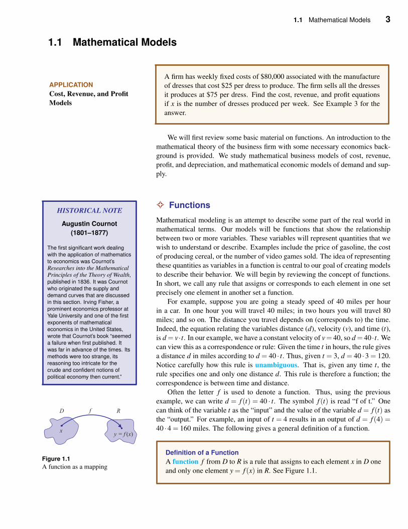
Figure 1.1
A function as a mapping
Often the letter f is used to denote a function. Thus, using the previous
example, we can write d = f (t) = 40 · t. The symbol f (t) is read “f of t.” One
can think of the variable t as the “input” and the value of the variable d = f (t) as
the “output.” For example, an input of t = 4 results in an output of d = f (4) =40 ·4 = 160 miles. The following gives a general definition of a function.
Definition of a Function
A function f from D to R is a rule that assigns to each element x in D one
and only one element y = f (x) in R. See Figure 1.1.
4 Chapter 1 Systems of Linear Equations and Models
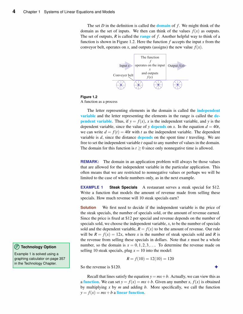
The set D in the definition is called the domain of f . We might think of the
domain as the set of inputs. We then can think of the values f (x) as outputs.
The set of outputs, R is called the range of f . Another helpful way to think of a
function is shown in Figure 1.2. Here the function f accepts the input x from the
conveyor belt, operates on x, and outputs (assigns) the new value f (x).
Figure 1.2
A function as a process
The letter representing elements in the domain is called the independent
variable and the letter representing the elements in the range is called the de-
pendent variable. Thus, if y = f (x), x is the independent variable, and y is the
dependent variable, since the value of y depends on x. In the equation d = 40t,
we can write d = f (t) = 40t with t as the independent variable. The dependent
variable is d, since the distance depends on the spent time t traveling. We are
free to set the independent variable t equal to any number of values in the domain.
The domain for this function is t ≥ 0 since only nonnegative time is allowed.
REMARK: The domain in an application problem will always be those values
that are allowed for the independent variable in the particular application. This
often means that we are restricted to nonnegative values or perhaps we will be
limited to the case of whole numbers only, as in the next example.
EXAMPLE 1 Steak Specials A restaurant serves a steak special for $12.
Write a function that models the amount of revenue made from selling these
specials. How much revenue will 10 steak specials earn?
Solution We first need to decide if the independent variable is the price of
the steak specials, the number of specials sold, or the amount of revenue earned.
Since the price is fixed at $12 per special and revenue depends on the number of
specials sold, we choose the independent variable, x, to be the number of specials
sold and the dependent variable, R = f (x) to be the amount of revenue. Our rule
will be R = f (x) = 12x, where x is the number of steak specials sold and R is
the revenue from selling these specials in dollars. Note that x must be a whole
number, so the domain is x = 0,1,2,3, . . .. To determine the revenue made on
selling 10 steak specials, plug x = 10 into the model:
R = f (10) = 12(10) = 120
So the revenue is $120. ✦
TTT©©© Technology Option
Example 1 is solved using a
graphing calculator on page 357
in the Technology Chapter.
Recall that lines satisfy the equation y=mx+b. Actually, we can view this as
a function. We can set y = f (x) = mx+b. Given any number x, f (x) is obtained
by multiplying x by m and adding b. More specifically, we call the function
y = f (x) = mx+b a linear function.
1.1 Mathematical Models 5
Definition of Linear Function
A linear function f is any function of the form,
y = f (x) = mx+b
where m and b are constants.
EXAMPLE 2 Linear Functions Which of the following functions are linear
functions?
a. y =−0.5x+12
b. 5y−2x = 10
c. y =1
x+2
d. y = x2
Solution
TTT©©© Technology Option
You can graph the functions on a
calculator to verify your results.
Linear functions will be a straight
line in any window.
a. This is a linear function. The slope is m =−0.5 and the y-intercept is b = 12.
b. Rewrite this function first as,
5y−2x = 10
5y = 2x+10
y =
(2
5
)
x+2
Now we see it is a linear function with m = 2/5 and b = 2.
c. This is not a linear function. Rewrite 1/x as x−1 and this shows that we do not
have a term mx and so this is not a linear function.
d. x is raised to the second power and so this is not a linear function. ✦
✧ Mathematical Modeling
When we use mathematical modeling we are attempting to describe some part of
the real world in mathematical terms, just as we have done for the distance trav-
eled and the revenue from selling meals. There are three steps in mathematical
modeling: formulation, mathematical manipulation, and evaluation.
First, on the basis of observations, we must state a question or formulate a hy-Formulation
pothesis. If the question or hypothesis is too vague, we need to make it precise.
If it is too ambitious, we need to restrict it or subdivide it into manageable parts.
Second, we need to identify important factors. We must decide which quantities
and relationships are important to answer the question and which can be ignored.
We then need to formulate a mathematical description. For example, each im-
portant quantity should be represented by a variable. Each relationship should
be represented by an equation, inequality, or other mathematical construct. If
6 Chapter 1 Systems of Linear Equations and Models
we obtain a function, say, y = f (x), we must carefully identify the input variable
x and the output variable y and the units for each. We should also indicate the
interval of values of the input variable for which the model is justified.
After the mathematical formulation, we then need to do some mathematical ma-Mathematical Manipulation
nipulation to obtain the answer to our original question. We might need to do a
calculation, solve an equation, or prove a theorem. Sometimes the mathematical
formulation gives us a mathematical problem that is impossible to solve. In such
a case, we will need to reformulate the question in a less ambitious manner.
Naturally, we need to check the answers given by the model with real data. WeEvaluation
normally expect the mathematical model to describe only a very limited aspect of
the world and to give only approximate answers. If the answers are wrong or not
accurate enough for our purposes, then we will need to identify the sources of the
model’s shortcomings. Perhaps we need to change the model entirely, or perhaps
we need to just make some refinements. In any case, this requires a new math-
ematical manipulation and evaluation. Thus, modeling often involves repeating
the three steps of formulation, mathematical manipulation, and evaluation.
We will next create linear mathematical models by finding equations that
relate cost, revenue, and profits of a manufacturing firm to the number of units
produced and sold.
✧ Cost, Revenue, and Profit
Any manufacturing firm has two types of costs: fixed and variable. Fixed costs
are those that do not depend on the amount of production. These costs include
real estate taxes, interest on loans, some management salaries, certain minimal
maintenance, and protection of plant and equipment. Variable costs depend on
the amount of production. They include the cost of material and labor. Total cost,
or simply cost, is the sum of fixed and variable costs:
cost = variable cost + fixed cost
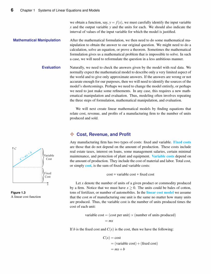
Figure 1.3
A linear cost function
Let x denote the number of units of a given product or commodity produced
by a firm. Notice that we must have x ≥ 0. The units could be bales of cotton,
tons of fertilizer, or number of automobiles. In the linear cost model we assume
that the cost m of manufacturing one unit is the same no matter how many units
are produced. Thus, the variable cost is the number of units produced times the
cost of each unit:
variable cost = (cost per unit)× (number of units produced)
= mx
If b is the fixed cost and C(x) is the cost, then we have the following:
C(x) = cost
= (variable cost)+(fixed cost)
= mx+b
1.1 Mathematical Models 7
Notice that we must have C(x)≥ 0. In the graph shown in Figure 1.3, we see that
the y-intercept is the fixed cost and the slope is the cost per item.
CONNECTION
What Are Costs?
Isn’t it obvious what the costs to a firm are? Apparently not. On July 15,
2002, Coca-Cola Company announced that it would begin treating stock-
option compensation as a cost, thereby lowering earnings. If all companies
in the Standard and Poor’s 500 stock index were to do the same, the earn-
ings for this index would drop by 23%.
Source: The Wall Street Journal, July 16, 2002
In the linear revenue model we assume that the price p of a unit sold by a
firm is the same no matter how many units are sold. (This is a reasonable as-
sumption if the number of units sold by the firm is small in comparison to the
total number sold by the entire industry.) Revenue is always the price per unit
times the number of units sold. Let x be the number of units sold. For conve-
nience, we always assume that the number of units sold equals the number of
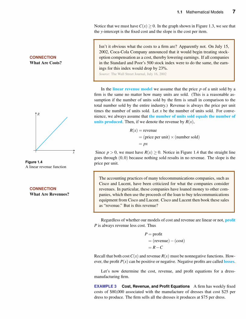
units produced. Then, if we denote the revenue by R(x),
R(x) = revenue
= (price per unit)× (number sold)
= px
Since p > 0, we must have R(x) ≥ 0. Notice in Figure 1.4 that the straight line
Figure 1.4
A linear revenue function
goes through (0,0) because nothing sold results in no revenue. The slope is the
price per unit.
CONNECTION
What Are Revenues?
The accounting practices of many telecommunications companies, such as
Cisco and Lucent, have been criticized for what the companies consider
revenues. In particular, these companies have loaned money to other com-
panies, which then use the proceeds of the loan to buy telecommunications
equipment from Cisco and Lucent. Cisco and Lucent then book these sales
as “revenue.” But is this revenue?
Regardless of whether our models of cost and revenue are linear or not, profit
P is always revenue less cost. Thus
P = profit
= (revenue)− (cost)
= R−C
Recall that both cost C(x) and revenue R(x) must be nonnegative functions. How-
ever, the profit P(x) can be positive or negative. Negative profits are called losses.
Let’s now determine the cost, revenue, and profit equations for a dress-
manufacturing firm.
EXAMPLE 3 Cost, Revenue, and Profit Equations A firm has weekly fixed
costs of $80,000 associated with the manufacture of dresses that cost $25 per
dress to produce. The firm sells all the dresses it produces at $75 per dress.
8 Chapter 1 Systems of Linear Equations and Models
a. Find the cost, revenue, and profit equations if x is the number of dresses
produced per week.
b. Make a table of values for cost, revenue, and profit for production levels of
1000, 1500, and 2000 dresses and discuss what is the table means.
Solution
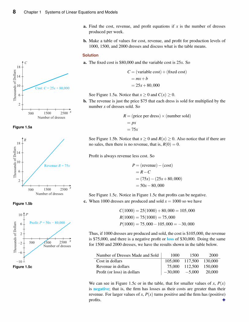
Figure 1.5a
a. The fixed cost is $80,000 and the variable cost is 25x. So
C = (variable cost)+(fixed cost)
= mx+b
= 25x+80,000
See Figure 1.5a. Notice that x≥ 0 and C(x)≥ 0.
Figure 1.5b
b. The revenue is just the price $75 that each dress is sold for multiplied by the
number x of dresses sold. So
R = (price per dress)× (number sold)
= px
= 75x
See Figure 1.5b. Notice that x≥ 0 and R(x)≥ 0. Also notice that if there are
no sales, then there is no revenue, that is, R(0) = 0.
Profit is always revenue less cost. So
P = (revenue)− (cost)
= R−C
= (75x)− (25x+80,000)
= 50x−80,000
See Figure 1.5c. Notice in Figure 1.5c that profits can be negative.
Figure 1.5c
c. When 1000 dresses are produced and sold x = 1000 so we have
C(1000) = 25(1000)+80,000 = 105,000
R(1000) = 75(1000) = 75,000
P(1000) = 75,000−105,000 =−30,000
Thus, if 1000 dresses are produced and sold, the cost is $105,000, the revenue
is $75,000, and there is a negative profit or loss of $30,000. Doing the same
for 1500 and 2000 dresses, we have the results shown in the table below.
Number of Dresses Made and Sold 1000 1500 2000
Cost in dollars 105,000 117,500 130,000
Revenue in dollars 75,000 112,500 150,000
Profit (or loss) in dollars −30,000 −5,000 20,000
We can see in Figure 1.5c or in the table, that for smaller values of x, P(x)is negative; that is, the firm has losses as their costs are greater than their
revenue. For larger values of x, P(x) turns positive and the firm has (positive)
profits. ✦
1.1 Mathematical Models 9
✧ Supply and Demand
In the previous discussion we assumed that the number of units produced and
sold by the given firm was small in comparison to the number sold by the indus-
try. Under this assumption it was reasonable to conclude that the price, p, was
constant and did not vary with the number x sold. But if the number of units
sold by the firm represented a large percentage of the number sold by the entire
industry, then trying to sell significantly more units could only be accomplished
by lowering the price of each unit. Since we just stated that the price effects
HISTORICAL NOTE
Adam Smith (1723–1790)
Adam Smith was a Scottish
political economist. His Inquiry
into the Nature and Causes of the
Wealth of Nations was one of the
earliest attempts to study the
development of industry and
commerce in Europe. That work
helped to create the modern
academic discipline of economics.
In the Western world, it is arguably
the most influential book on the
subject ever published.
the number sold, you would expect the price to be the independent variable and
thus graphed on the horizontal axis. However, by custom, the price is graphed
on the vertical axis and the quantity x on the horizontal axis. This convention
was started by English economist Alfred Marshall (1842–1924) in his important
book, Principles of Economics. We will abide by this custom in this text.
For most items the relationship between quantity and price is a decreasing
function (there are some exceptions to this rule, such as certain luxury goods,
medical care, and higher eduction, to name a few). That is, for the number
of items to be sold to increase, the price must decrease. We assume now for
mathematical convenience that this relationship is linear. Then the graph of this
equation is a straight line that slopes downward as shown in Figure 1.6.
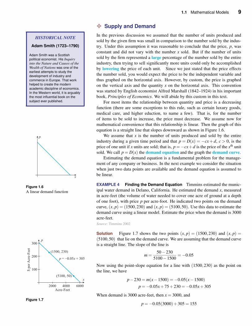
Figure 1.6
A linear demand function
We assume that x is the number of units produced and sold by the entire
industry during a given time period and that p = D(x) = −cx+ d, c > 0, is the
price of one unit if x units are sold; that is, p =−cx+d is the price of the xth unit
sold. We call p = D(x) the demand equation and the graph the demand curve.
Estimating the demand equation is a fundamental problem for the manage-
ment of any company or business. In the next example we consider the situation
when just two data points are available and the demand equation is assumed to
be linear.
EXAMPLE 4 Finding the Demand Equation Timmins estimated the munic-
ipal water demand in Delano, California. He estimated the demand x, measured
in acre-feet (the volume of water needed to cover one acre of ground at a depth
of one foot), with price p per acre-foot. He indicated two points on the demand
curve, (x, p) = (1500,230) and (x, p) = (5100,50). Use this data to estimate the
demand curve using a linear model. Estimate the price when the demand is 3000
acre-feet.
Source: Timmins 2002
Solution Figure 1.7 shows the two points (x, p) = (1500,230) and (x, p) =(5100,50) that lie on the demand curve. We are assuming that the demand curve
Figure 1.7
is a straight line. The slope of the line is
m =50−230
5100−1500=−0.05
Now using the point-slope equation for a line with (1500,230) as the point on
the line, we have
p−230 = m(x−1500) =−0.05(x−1500)
p =−0.05x+75+230 =−0.05x+305
When demand is 3000 acre-feet, then x = 3000, and
p =−0.05(3000)+305 = 155
10 Chapter 1 Systems of Linear Equations and Models
or $155 per acre-foot. Thus, according to this model, if 3000 acre-feet is de-
manded, the price of each acre-foot will be $155. ✦
CONNECTION
Demand for Apartments
The figure shows that during the mi-
nor recession of 2001, vacancy rates for
apartments increased, that is, the de-
mand for apartments decreased. Notice
in the figure that as demand for apart-
ments decreased, rents also decreased.
For example, in San Francisco’s South
Beach area, a two-bedroom apartment
that had rented for $3000 a month two
years before saw the rent drop to $2100
a month.Source: Wall Street Journal, April 11, 2002
The supply equation p = S(x) gives the price p necessary for suppliers to
make available x units to the market. The graph of this equation is called the sup-
ply curve. A reasonable supply curve rises, moving from left to right, because
the suppliers of any product naturally want to sell more if the price is higher.
(See Shea 1993 who looked at a large number of industries and determined that
the supply curve does indeed slope upward.) If the supply curve is linear, then
as shown in Figure 1.8, the graph is a line sloping upward. Note the positive
y-intercept. The y-intercept represents the choke point or lowest price a supplier
is willing to accept.
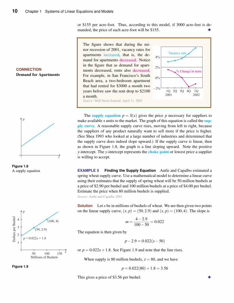
Figure 1.8
A supply equation EXAMPLE 5 Finding the Supply Equation Antle and Capalbo estimated a
spring wheat supply curve. Use a mathematical model to determine a linear curve
using their estimates that the supply of spring wheat will be 50 million bushels at
a price of $2.90 per bushel and 100 million bushels at a price of $4.00 per bushel.
Estimate the price when 80 million bushels is supplied.
Source: Antle and Capalbo 2001
Solution Let x be in millions of bushels of wheat. We are then given two points
on the linear supply curve, (x, p) = (50,2.9) and (x, p) = (100,4). The slope is
Figure 1.9
m =4−2.9
100−50= 0.022
The equation is then given by
p−2.9 = 0.022(x−50)
or p = 0.022x+1.8. See Figure 1.9 and note that the line rises.
When supply is 80 million bushels, x = 80, and we have
p = 0.022(80)+1.8 = 3.56
This gives a price of $3.56 per bushel. ✦
1.1 Mathematical Models 11
CONNECTION
Supply of Cotton
On May 2, 2002, the U.S. House of Representatives passed a farm bill
that promises billions of dollars in subsidies to cotton farmers. With the
prospect of a greater supply of cotton, cotton prices dropped 1.36 cents to
33.76 cents per pound.
Source: The Wall Street Journal, May 3, 2002.
✧ Straight-Line Depreciation
Many assets, such as machines or buildings, have a finite useful life and further-
more depreciate in value from year to year. For purposes of determining profits
and taxes, various methods of depreciation can be used. In straight-line depre-
ciation we assume that the value V of the asset is given by a linear equation in
time t, say, V = mt + b. The slope m must be negative since the value of the
asset decreases over time. However, if asked about the "‘rate of depreciation"’,
the answer is the absolute value of the slope, since the rate of depreciation is
understood to be negative. The y-intercept is the initial value of the item and the
slope gives the rate of depreciation (how much the item decreases in value per
time period).
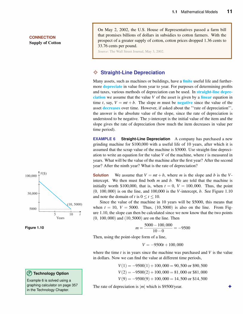
EXAMPLE 6 Straight-Line Depreciation A company has purchased a new
grinding machine for $100,000 with a useful life of 10 years, after which it is
assumed that the scrap value of the machine is $5000. Use straight-line depreci-
ation to write an equation for the value V of the machine, where t is measured in
years. What will be the value of the machine after the first year? After the second
year? After the ninth year? What is the rate of depreciation?
Solution We assume that V = mt + b, where m is the slope and b is the V -
intercept. We then must find both m and b. We are told that the machine is
initially worth $100,000, that is, when t = 0, V = 100,000. Thus, the point
(0, 100,000) is on the line, and 100,000 is the V -intercept, b. See Figure 1.10
and note the domain of t is 0≤ t ≤ 10.
Figure 1.10
Since the value of the machine in 10 years will be $5000, this means that
when t = 10, V = 5000. Thus, (10,5000) is also on the line. From Fig-
ure 1.10, the slope can then be calculated since we now know that the two points
(0, 100,000) and (10,5000) are on the line. Then
m =5000−100,000
10−0=−9500
Then, using the point-slope form of a line,
V =−9500t +100,000
where the time t is in years since the machine was purchased and V is the value
in dollars. Now we can find the value at different time periods,
TTT©©© Technology Option
Example 6 is solved using a
graphing calculator on page 357
in the Technology Chapter.
V (1) =−9500(1)+100,000 = 90,500 or $90,500
V (2) =−9500(2)+100,000 = 81,000 or $81,000
V (9) =−9500(9)+100,000 = 14,500 or $14,500
The rate of depreciation is |m| which is $9500/year. ✦
12 Chapter 1 Systems of Linear Equations and Models
Self-Help Exercises 1.1
1. Rogers and Akridge of Purdue University studied
fertilizer plants in Indiana. For a typical medium-
sized plant they estimated fixed costs at $400,000
and estimated the cost of each ton of fertilizer was
$200 to produce. The plant sells its fertilizer output
at $250 per ton.
a. Find and graph the cost, revenue, and profit
equations.
b. Determine the cost, revenue, and profits when
the number of tons produced and sold is 5000,
7000, and 9000 tons.Source: Rogers and Akridge 1996
2. The excess supply and demand curves for wheat
worldwide were estimated by Schmitz and cowork-
ers to be
Supply: p = 7x−400
Demand: p = 510−3.5x
where p is price in dollars per metric ton and x is in
millions of metric tons. Excess demand refers to the
excess of wheat that producer countries have over
their own consumption. Graph these two functions.
Find the prices for the supply and demand models
when x is 70 million metric tons. Is the price for
supply or demand larger? Repeat these questions
when x is 100 million metric tons.
Source: Schmitz, Sigurdson, and Doering 1986
1.1 Exercises
In Exercises 1 and 2 you are given the cost per item and
the fixed costs. Assuming a linear cost model, find the
cost equation, where C is cost and x is the number pro-
duced.
1. Cost per item = $3, fixed cost=$10,000
2. Cost per item = $6, fixed cost=$14,000
In Exercises 3 and 4 you are given the price of each
item, which is assumed to be constant. Find the revenue
equation, where R is revenue and x is the number sold.
3. Price per item = $5
4. Price per item = $.10
5. Using the cost equation found in Exercise 1 and the
revenue equation found in Exercise 3, find the profit
equation for P, assuming that the number produced
equals the number sold.
6. Using the cost equation found in Exercise 2 and the
revenue equation found in Exercise 4, find the profit
equation for P, assuming that the number produced
equals the number sold.
In Exercises 7 to 10, find the demand equation using the
given information.
7. A company finds it can sell 10 items at a price of $8
each and sell 15 items at a price of $6 each.
8. A company finds it can sell 40 items at a price of
$60 each and sell 60 items at a price of $50 each.
9. A company finds that at a price of $35, a total of
100 items will be sold. If the price is lowered by $5,
then 20 additional items will be sold.
10. A company finds that at a price of $200, a total of
30 items will be sold. If the price is raised $50, then
10 fewer items will be sold.
In Exercises 11 to 14, find the supply equation using the
given information.
11. A supplier will supply 50 items to the market if the
price is $95 per item and supply 100 items if the
price is $175 per item.
12. A supplier will supply 1000 items to the market if
the price is $3 per item and supply 2000 items if the
price is $4 per item.
13. At a price of $60 per item, a supplier will supply 10
of these items. If the price increases by $20, then 4
additional items will be supplied.
1.1 Mathematical Models 13
14. At a price of $800 per item, a supplier will supply
90 items. If the price decreases by $50, then the
supplier will supply 20 fewer items.
In Exercises 15 to 18, find the depreciation equation and
corresponding domain using the given information.
15. A calculator is purchased for $130 and the value de-
creases by $15 per year for 7 years.
16. A violin bow is purchased for $50 and the value de-
creases by $5 per year for 6 years.
17. A car is purchased for $15,000 and is sold for $6000
six years later.
18. A car is purchased for $32,000 and is sold for
$23,200 eight years later.
Applications
19. Wood Chipper Cost A contractor needs to rent a
wood chipper for a day for $150 plus $10 per hour.
Find the cost function.
20. Truck Rental Cost A builder needs to rent a dump
truck for a day for $75 plus $.40 per mile. Find the
cost function.
21. Sewing Machine Cost A shirt manufacturer is con-
sidering purchasing a sewing machine for $91,000
and it will cost $2 to sew each of their standard
shirts. Find the cost function.
22. Copying Cost At Lincoln Library there are two
ways to pay for copying. You can pay 5 cents a
copy, or you can buy a plastic card for $5 and then
pay 3 cents a copy. Let x be the number of copies
you make. Write an equation for your costs for each
way of paying.
23. Assume that the linear cost model applies and fixed
costs are $1000. If the total cost of producing 800
items is $5000, find the cost equation.
24. Assume that the linear cost model applies. If the to-
tal cost of producing 1000 items at $3 each is $5000,
find the cost equation.
25. When 50 silver beads are ordered they cost $1.25
each. If 100 silver beads are ordered, they cost
$1.00 each. How much will each silver bead cost
if 250 are ordered?
26. You find that when you order 75 magnets, the aver-
age cost per magnet is $.90 and when you order 200
magnets, the average cost per magnet is $.80. What
is the cost equation for these custom magnets?
27. Assume that the linear revenue model applies. If the
total revenue from selling 600 items is $7200, find
the revenue equation.
28. Assume that the linear revenue model applies. If the
total revenue from selling 1000 items is $8000, find
the revenue equation.
29. Assume that the linear cost and revenue model ap-
plies. An item sells for $10. If fixed costs are $2000
and profits are $7000 when 1000 items are made and
sold, find the cost equation.
30. Assume that the linear cost and revenue models ap-
plies. An item that costs $3 to make sells for $6.
If profits of $5000 are made when 2000 items are
made and sold, find the cost equation.
31. Assume that the linear cost and revenue models ap-
plies. Each additional item costs $3 to make. If
fixed costs are $1000 and profits are $7000 when
1000 items are made and sold, find the revenue
equation.
32. Assume that the linear cost and revenue models ap-
plies. An item costs $7 to make. If fixed costs are
$1500 and profits are $1700 when 200 items are
made and sold, find the revenue equation.
33. Demand for Blueberries A grocery store sells 27
packages of blueberries daily when the price is
$3.18 per package. If the price is decreased by $.25
per package, then the store will sell an additional 5
packages every day. What is the demand equation
for blueberries?
34. Demand for Bagels A bakery sells 124 bagels daily
when the price is $1.50 per bagel. If the price is
increased by $.50, the bakery will sell 25 fewer
bagels. What is the demand equation for bagels?
35. Supply of Basil A farmer is willing to supply 15
packages of organic basil to a market for $2 per
package. If the market offers the farmer $1 more
per package, the farmer will supply 20 more pack-
ages of organic basil. What is the supply equation
for organic basil?
36. Supply of Roses A grower is willing to supply 200
long-stemmed roses per week to a florist for $.85
14 Chapter 1 Systems of Linear Equations and Models
per rose. If the florist offers the grower $.20 less
per rose, then the grower will supply 50 fewer roses.
What is the supply equation for these long-stemmed
roses?
37. Machine Depreciation Consider a new machine
that costs $50,000 and has a useful life of nine years
and a scrap value of $5000. Using straight-line de-
preciation, find the equation for the value V in terms
of t, where t is in years. Find the value after one year
and after five years.
38. Building Depreciation A new building that costs
$1,100,000 has a useful life of 50 years and a scrap
value of $100,000. Using straight-line depreciation,
find the equation for the value V in terms of t, where
t is in years. Find the value after 1 year, after 2
years, and after 40 years.
Referenced Applications
39. Cotton Ginning Cost Misra and colleagues esti-
mated the cost function for the ginning industry in
the Southern High Plains of Texas. They give a (to-
tal) cost function C by C(x) = 21x+674,000, where
C is in dollars and x is the number of bales of cotton.
Find the fixed and variable costs.
Source: Misra, McPeek, and Segarra 2000
40. Fishery Cost The cost function for wild crayfish
was estimated by Bell to be a function C(x), where
x is the number of millions of pounds of crayfish
caught and C is the cost in millions of dollars. Two
points that are on the graph are (x,C) = (8,0.157)and (x,C) = (10,0.190). Using this information and
assuming a linear model, determine a cost function.
Source: Bell 1986
41. Fender Costs Saur and colleagues did a care-
ful study of the cost of manufacturing automo-
bile fenders. The fenders were made from five
different materials: steel, aluminum, and three
injection-molded polymer blends: rubber-modified
polypropylene (RMP), nylon-polyphenylene oxide
(NPN), and polycarbonate-polybutylene terephtha-
late (PPT). The following table gives the fixed and
variable costs of manufacturing each pair of fenders.
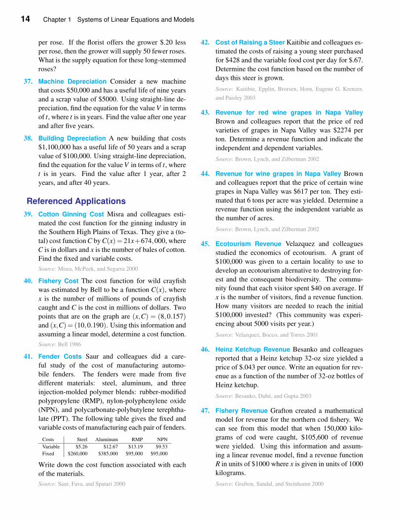
Costs Steel Aluminum RMP NPN
Variable $5.26 $12.67 $13.19 $9.53
Fixed $260,000 $385,000 $95,000 $95,000
Write down the cost function associated with each
of the materials.
Source: Saur, Fava, and Spatari 2000
42. Cost of Raising a Steer Kaitibie and colleagues es-
timated the costs of raising a young steer purchased
for $428 and the variable food cost per day for $.67.
Determine the cost function based on the number of
days this steer is grown.
Source: Kaitibie, Epplin, Brorsen, Horn, Eugene G. Krenzer,
and Paisley 2003
43. Revenue for red wine grapes in Napa Valley
Brown and colleagues report that the price of red
varieties of grapes in Napa Valley was $2274 per
ton. Determine a revenue function and indicate the
independent and dependent variables.
Source: Brown, Lynch, and Zilberman 2002
44. Revenue for wine grapes in Napa Valley Brown
and colleagues report that the price of certain wine
grapes in Napa Valley was $617 per ton. They esti-
mated that 6 tons per acre was yielded. Determine a
revenue function using the independent variable as
the number of acres.
Source: Brown, Lynch, and Zilberman 2002
45. Ecotourism Revenue Velazquez and colleagues
studied the economics of ecotourism. A grant of
$100,000 was given to a certain locality to use to
develop an ecotourism alternative to destroying for-
est and the consequent biodiversity. The commu-
nity found that each visitor spent $40 on average. If
x is the number of visitors, find a revenue function.
How many visitors are needed to reach the initial
$100,000 invested? (This community was experi-
encing about 5000 visits per year.)
Source: Velazquez, Bocco, and Torres 2001
46. Heinz Ketchup Revenue Besanko and colleagues
reported that a Heinz ketchup 32-oz size yielded a
price of $.043 per ounce. Write an equation for rev-
enue as a function of the number of 32-oz bottles of
Heinz ketchup.
Source: Besanko, Dubé, and Gupta 2003
47. Fishery Revenue Grafton created a mathematical
model for revenue for the northern cod fishery. We
can see from this model that when 150,000 kilo-
grams of cod were caught, $105,600 of revenue
were yielded. Using this information and assum-
ing a linear revenue model, find a revenue function
R in units of $1000 where x is given in units of 1000
kilograms.
Source: Grafton, Sandal, and Steinhamn 2000
1.1 Mathematical Models 15
48. Shrimp Profit Kekhora and McCann estimated a
cost function for a shrimp production function in
Thailand. They gave the fixed costs per hectare of
$1838 and the variable costs per hectare of $14,183.
The revenue per hectare was given as $26,022
a. Determine the total cost for 1 hectare.
b. Determine the profit for 1 hectare.
Source: Kekhora and McCann 2003
49. Rice Production Profit Kekhora and McCann esti-
mated a cost function for the rice production func-
tion in Thailand. They gave the fixed costs per
hectare of $75 and the variable costs per hectare of
$371. The revenue per hectare was given as $573.
a. Determine the total cost for 1 hectare.
b. Determine the profit for 1 hectare.
Source: Kekhora and McCann 2003
50. Profit for Small Fertilizer Plants In 1996 Rogers
and Akridge of Purdue University studied fertilizer
plants in Indiana. For a typical small-sized plant
they estimated fixed costs at $235,487 and estimated
that it cost $206.68 to produce each ton of fertilizer.
The plant sells its fertilizer output at $266.67 per
ton. Find the cost, revenue, and profit equations.
Source: Rogers and Akridge 1996
51. Profit for Large Fertilizer Plants In 1996 Rogers
and Akridge of Purdue University studied fertilizer
plants in Indiana. For a typical large-sized plant
they estimated fixed costs at $447,917 and estimated
that it cost $209.03 to produce each ton of fertilizer.
The plant sells its fertilizer output at $266.67 per
ton. Find the cost, revenue, and profit equations.
Source: Rogers and Akridge 1996
52. Demand for Recreation Shafer and others esti-
mated a demand curve for recreational power boat-
ing in a number of bodies of water in Pennsylvania.
They estimated the price p of a power boat trip in-
cluding rental cost of boat, cost of fuel, and rental
cost of equipment. For the Lake Erie/Presque Isle
Bay Area they collected data indicating that for a
price (cost) of $144, individuals made 10 trips, and
for a price of $50, individuals made 20 trips. As-
suming a linear model determine the demand curve.
For 15 trips, what was the cost?
Source: Shafer, Upneja, Seo, and Yoon 2000
53. Demand for Recreation Shafer and others esti-
mated a demand curve for recreational power boat-
ing in a number of bodies of water in Pennsylvania.
They estimated the price p of a power boat trip in-
cluding rental cost of boat, cost of fuel, and rental
cost of equipment. For the Three Rivers Area they
collected data indicating that for a price (cost) of
$99, individuals made 10 trips, and for a price of
$43, individuals made 20 trips. Assuming a linear
model determine the demand curve. For 15 trips,
what was the cost?
Source: Shafer, Upneja, Seo, and Yoon 2000
54. Demand for Cod Grafton created a mathematical
model for demand for the northern cod fishery. We
can see from this model that when 100,000 kilo-
grams of cod were caught the price was $.81 per
kilogram and when 200,000 kilograms of cod were
caught the price was $.63 per kilogram. Using this
information and assuming a linear demand model,
find a demand function.
Source: Grafton, Sandal, and Steinhamn 2000
55. Demand for Rice Suzuki and Kaiser estimated
the demand equation for rice in Japan to be p =1,195,789− 0.1084753x, where x is in tons of rice
and p is in yen per ton. In 1995, the quantity of rice
consumed in Japan was 8,258,000 tons.
a. According to the demand equation, what was the
price in yen per ton?
b. What happens to the price of a ton of rice when
the demand increases by 1 ton. What has this
number to do with the demand equation?
Source: Suzuki and Kaiser 1998
56. Supply of Childcare Blau and Mocan gathered data
over a number of states and estimated a supply
curve that related quality of child care with price.
For quality q of child care they developed an in-
dex of quality and for price p they used their own
units. In their graph they gave q = S(p), that is, the
price was the independent variable. On this graph
we see the following points: (p,q) = (1,2.6) and
(p,q) = (3,5.5). Use this information and assum-
ing a linear model, determine the supply curve.
Source: Blau and Mocan 2002
57. Oil Production Technology The economics of con-
version to saltwater injection for inactive wells in
Texas was studied by D’Unger and coworkers. (By
injecting saltwater into the wells, pressure is applied
to the oil field, and oil and gas are forced out to be
recovered.) The expense of a typical well conver-
sion was estimated to be $31,750. The monthly rev-
enue as a result of the conversion was estimated to
16 Chapter 1 Systems of Linear Equations and Models
be $2700. If x is the number of months the well op-
erates after conversion, determine a revenue func-
tion as a function of x. How many months of op-
eration would it take to recover the initial cost of
conversion?
Source: D’Unger, Chapman, and Carr 1996
58. Rail Freight In a report of the Federal Trade Com-
mission (FTC) an example is given in which the
Portland, Oregon, mill price of 50,000 board square
feet of plywood is $3525 and the rail freight is
$0.3056 per mile.
a. If a customer is located x rail miles from this
mill, write an equation that gives the total freight
f charged to this customer in terms of x for de-
livery of 50,000 board square feet of plywood.
b. Write a (linear) equation that gives the total c
charged to a customer x rail miles from the mill
for delivery of 50,000 board square feet of ply-
wood. Graph this equation.
c. In the FTC report, a delivery of 50,000 board
square feet of plywood from this mill is made
to New Orleans, Louisiana, 2500 miles from the
mill. What is the total charge?
Source: Gilligan 1992
Extensions
59. Understanding the Revenue Equation Assuming
a linear revenue model, explain in a complete sen-
tence where you expect the y-intercept to be. Give a
reason for your answer.
60. Understanding the Cost and Profit Equations As-
suming a linear cost and revenue model, explain
in complete sentences where you expect the y-
intercepts to be for the cost and profit equations.
Give reasons for your answers.
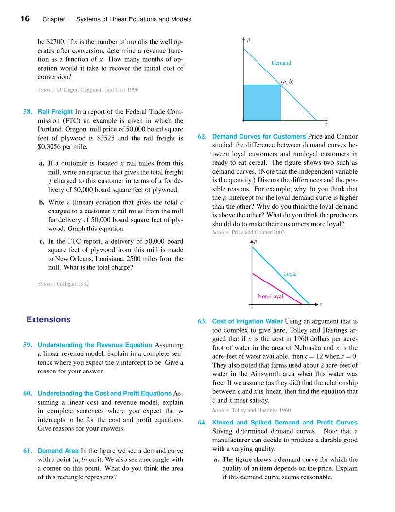
61. Demand Area In the figure we see a demand curve
with a point (a,b) on it. We also see a rectangle with
a corner on this point. What do you think the area
of this rectangle represents?
62. Demand Curves for Customers Price and Connor
studied the difference between demand curves be-
tween loyal customers and nonloyal customers in
ready-to-eat cereal. The figure shows two such as
demand curves. (Note that the independent variable
is the quantity.) Discuss the differences and the pos-
sible reasons. For example, why do you think that
the p-intercept for the loyal demand curve is higher
than the other? Why do you think the loyal demand
is above the other? What do you think the producers
should do to make their customers more loyal?Source: Price and Conner 2003
p
x
Loyal
Non-Loyal
63. Cost of Irrigation Water Using an argument that is
too complex to give here, Tolley and Hastings ar-
gued that if c is the cost in 1960 dollars per acre-
foot of water in the area of Nebraska and x is the
acre-feet of water available, then c= 12 when x= 0.
They also noted that farms used about 2 acre-feet of
water in the Ainsworth area when this water was
free. If we assume (as they did) that the relationship
between c and x is linear, then find the equation that
c and x must satisfy.
Source: Tolley and Hastings 1960
64. Kinked and Spiked Demand and Profit Curves
Stiving determined demand curves. Note that a
manufacturer can decide to produce a durable good
with a varying quality.
a. The figure shows a demand curve for which the
quality of an item depends on the price. Explain
if this demand curve seems reasonable.
1.1 Mathematical Models 17
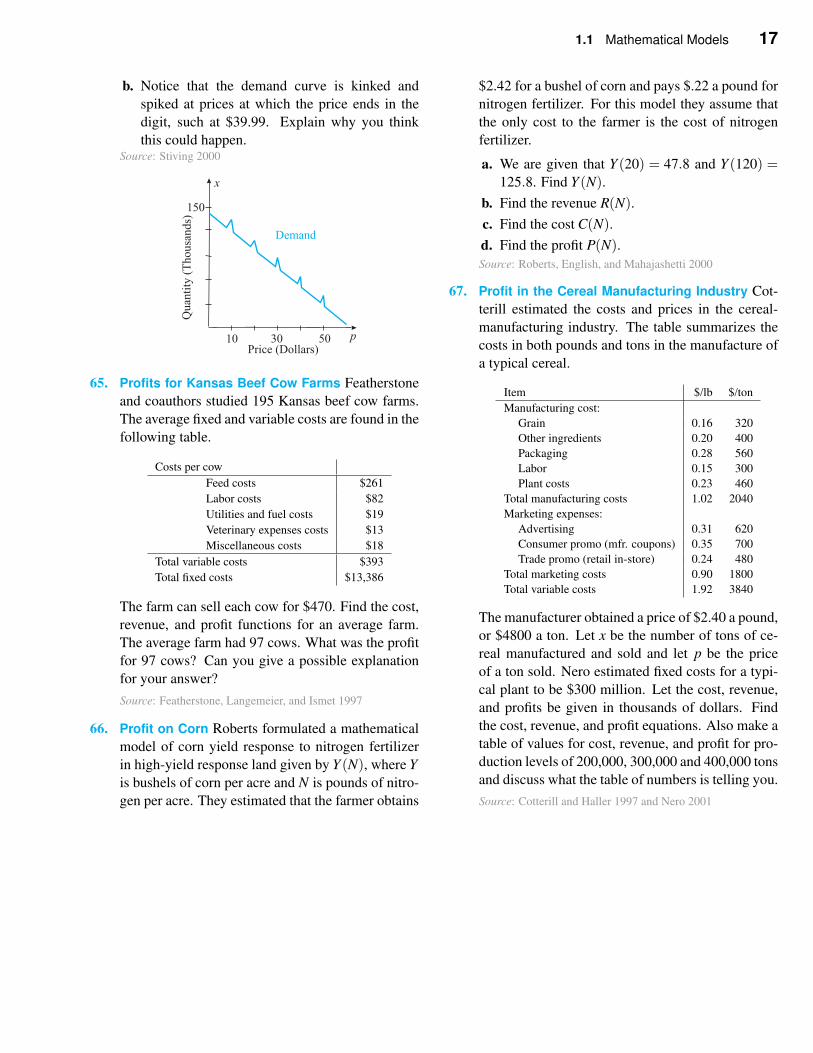
b. Notice that the demand curve is kinked and
spiked at prices at which the price ends in the
digit, such at $39.99. Explain why you think
this could happen.Source: Stiving 2000
65. Profits for Kansas Beef Cow Farms Featherstone
and coauthors studied 195 Kansas beef cow farms.
The average fixed and variable costs are found in the
following table.
Costs per cow
Feed costs $261
Labor costs $82
Utilities and fuel costs $19
Veterinary expenses costs $13
Miscellaneous costs $18
Total variable costs $393
Total fixed costs $13,386
The farm can sell each cow for $470. Find the cost,
revenue, and profit functions for an average farm.
The average farm had 97 cows. What was the profit
for 97 cows? Can you give a possible explanation
for your answer?
Source: Featherstone, Langemeier, and Ismet 1997
66. Profit on Corn Roberts formulated a mathematical
model of corn yield response to nitrogen fertilizer
in high-yield response land given by Y (N), where Y
is bushels of corn per acre and N is pounds of nitro-
gen per acre. They estimated that the farmer obtains
$2.42 for a bushel of corn and pays $.22 a pound for
nitrogen fertilizer. For this model they assume that
the only cost to the farmer is the cost of nitrogen
fertilizer.
a. We are given that Y (20) = 47.8 and Y (120) =125.8. Find Y (N).
b. Find the revenue R(N).
c. Find the cost C(N).
d. Find the profit P(N).
Source: Roberts, English, and Mahajashetti 2000
67. Profit in the Cereal Manufacturing Industry Cot-
terill estimated the costs and prices in the cereal-
manufacturing industry. The table summarizes the
costs in both pounds and tons in the manufacture of
a typical cereal.
Item $/lb $/ton
Manufacturing cost:
Grain 0.16 320
Other ingredients 0.20 400
Packaging 0.28 560
Labor 0.15 300
Plant costs 0.23 460
Total manufacturing costs 1.02 2040
Marketing expenses:
Advertising 0.31 620
Consumer promo (mfr. coupons) 0.35 700
Trade promo (retail in-store) 0.24 480
Total marketing costs 0.90 1800
Total variable costs 1.92 3840
The manufacturer obtained a price of $2.40 a pound,
or $4800 a ton. Let x be the number of tons of ce-
real manufactured and sold and let p be the price
of a ton sold. Nero estimated fixed costs for a typi-
cal plant to be $300 million. Let the cost, revenue,
and profits be given in thousands of dollars. Find
the cost, revenue, and profit equations. Also make a
table of values for cost, revenue, and profit for pro-
duction levels of 200,000, 300,000 and 400,000 tons
and discuss what the table of numbers is telling you.
Source: Cotterill and Haller 1997 and Nero 2001
18 Chapter 1 Systems of Linear Equations and Models
Solutions to Self-Help Exercises 1.1
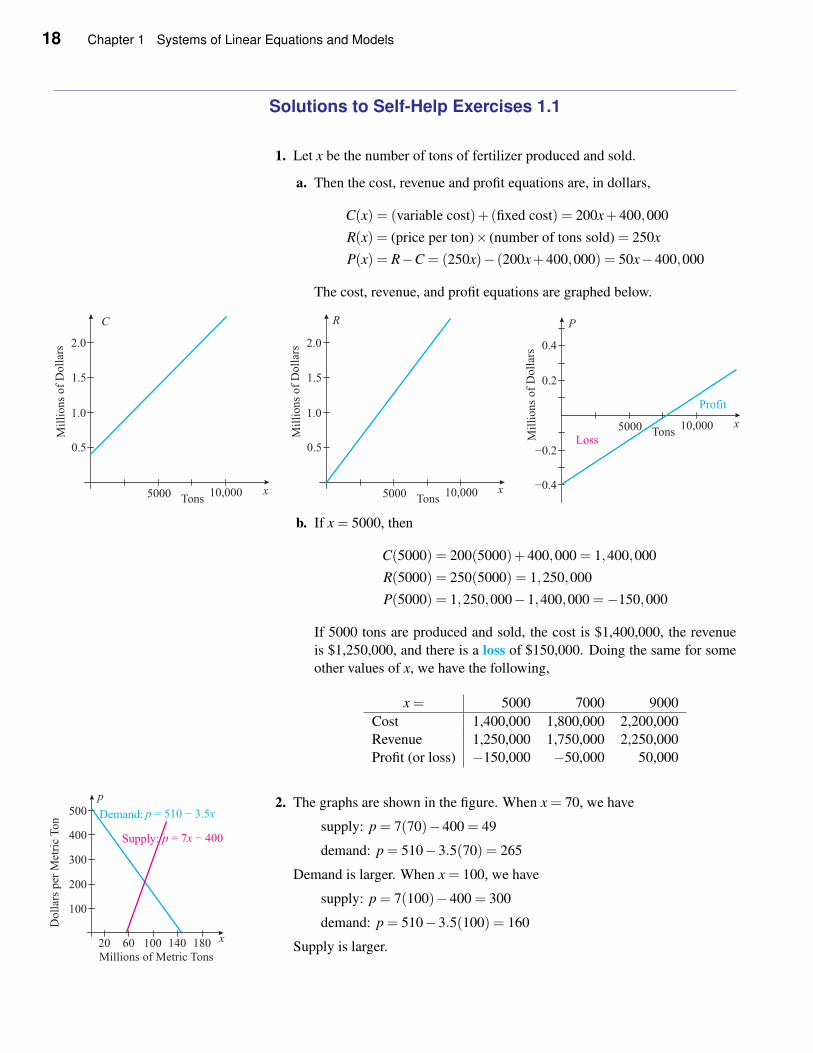
1. Let x be the number of tons of fertilizer produced and sold.
a. Then the cost, revenue and profit equations are, in dollars,
C(x) = (variable cost)+(fixed cost) = 200x+400,000
R(x) = (price per ton)× (number of tons sold) = 250x
P(x) = R−C = (250x)− (200x+400,000) = 50x−400,000
The cost, revenue, and profit equations are graphed below.
b. If x = 5000, then
C(5000) = 200(5000)+400,000 = 1,400,000
R(5000) = 250(5000) = 1,250,000
P(5000) = 1,250,000−1,400,000 =−150,000
If 5000 tons are produced and sold, the cost is $1,400,000, the revenue
is $1,250,000, and there is a loss of $150,000. Doing the same for some
other values of x, we have the following,
x = 5000 7000 9000
Cost 1,400,000 1,800,000 2,200,000
Revenue 1,250,000 1,750,000 2,250,000
Profit (or loss) −150,000 −50,000 50,000
2. The graphs are shown in the figure. When x = 70, we have
supply: p = 7(70)−400 = 49
demand: p = 510−3.5(70) = 265
Demand is larger. When x = 100, we have
supply: p = 7(100)−400 = 300
demand: p = 510−3.5(100) = 160
Supply is larger.
1.2 Systems of Linear Equations 19
1.2 Systems of Linear Equations
APPLICATION
Cost, Revenue, and Profit
Models
In Example 3 in the last section we found the cost and revenue equations
in the dress-manufacturing industry. Let x be the number of dresses made
and sold. Recall that cost and revenue functions were found to be C(x) =25x+ 80,000 and R(x) = 75x. Find the point at which the profit is zero.
See Example 2 for the answer.
We now begin to look at systems of linear equations in many unknowns. In
this section we first consider systems of two linear equations in two unknowns.
We will see that solutions of such a system have a variety of applications.
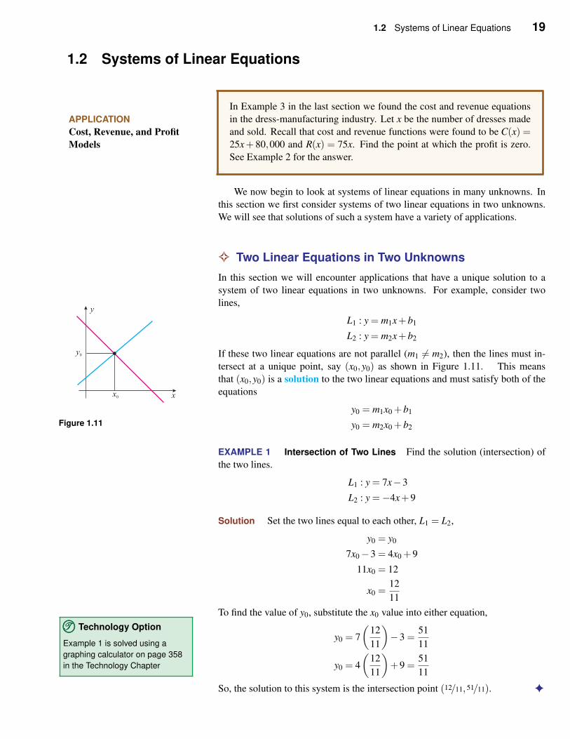
✧ Two Linear Equations in Two Unknowns
In this section we will encounter applications that have a unique solution to a
system of two linear equations in two unknowns. For example, consider two
lines,
L1 : y = m1x+b1
L2 : y = m2x+b2
If these two linear equations are not parallel (m1 6= m2), then the lines must in-
tersect at a unique point, say (x0,y0) as shown in Figure 1.11. This means
Figure 1.11
that (x0,y0) is a solution to the two linear equations and must satisfy both of the
equations
y0 = m1x0 +b1
y0 = m2x0 +b2
EXAMPLE 1 Intersection of Two Lines Find the solution (intersection) of
the two lines.
L1 : y = 7x−3
L2 : y =−4x+9
Solution Set the two lines equal to each other, L1 = L2,
y0 = y0
7x0−3 = 4x0 +9
11x0 = 12
x0 =12
11
To find the value of y0, substitute the x0 value into either equation,
TTT©©© Technology Option
Example 1 is solved using a
graphing calculator on page 358
in the Technology Chapter
y0 = 7
(12
11
)
−3 =51
11
y0 = 4
(12
11
)
+9 =51
11
So, the solution to this system is the intersection point (12/11, 51/11). ✦
20 Chapter 1 Systems of Linear Equations and Models
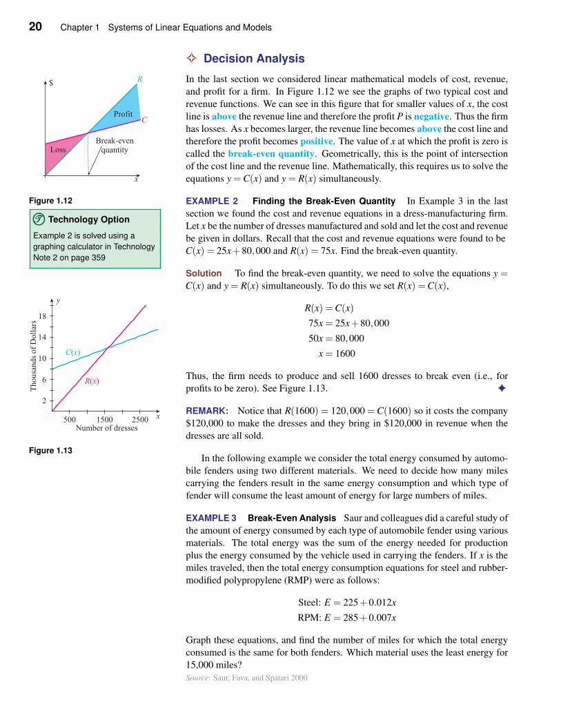
✧ Decision Analysis
In the last section we considered linear mathematical models of cost, revenue,
and profit for a firm. In Figure 1.12 we see the graphs of two typical cost and
revenue functions. We can see in this figure that for smaller values of x, the cost
line is above the revenue line and therefore the profit P is negative. Thus the firm
has losses. As x becomes larger, the revenue line becomes above the cost line and
therefore the profit becomes positive. The value of x at which the profit is zero is
called the break-even quantity. Geometrically, this is the point of intersection
of the cost line and the revenue line. Mathematically, this requires us to solve the
equations y =C(x) and y = R(x) simultaneously.
Figure 1.12 EXAMPLE 2 Finding the Break-Even Quantity In Example 3 in the last
section we found the cost and revenue equations in a dress-manufacturing firm.
Let x be the number of dresses manufactured and sold and let the cost and revenue
be given in dollars. Recall that the cost and revenue equations were found to be
TTT©©© Technology Option
Example 2 is solved using a
graphing calculator in Technology
Note 2 on page 359C(x) = 25x+80,000 and R(x) = 75x. Find the break-even quantity.
Solution To find the break-even quantity, we need to solve the equations y =C(x) and y = R(x) simultaneously. To do this we set R(x) =C(x),
R(x) =C(x)
75x = 25x+80,000
50x = 80,000
x = 1600
Thus, the firm needs to produce and sell 1600 dresses to break even (i.e., for
profits to be zero). See Figure 1.13. ✦
Figure 1.13
REMARK: Notice that R(1600) = 120,000 =C(1600) so it costs the company
$120,000 to make the dresses and they bring in $120,000 in revenue when the
dresses are all sold.
In the following example we consider the total energy consumed by automo-
bile fenders using two different materials. We need to decide how many miles
carrying the fenders result in the same energy consumption and which type of
fender will consume the least amount of energy for large numbers of miles.
EXAMPLE 3 Break-Even Analysis Saur and colleagues did a careful study of
the amount of energy consumed by each type of automobile fender using various
materials. The total energy was the sum of the energy needed for production
plus the energy consumed by the vehicle used in carrying the fenders. If x is the
miles traveled, then the total energy consumption equations for steel and rubber-
modified polypropylene (RMP) were as follows:
Steel: E = 225+0.012x
RPM: E = 285+0.007x
Graph these equations, and find the number of miles for which the total energy
consumed is the same for both fenders. Which material uses the least energy for
15,000 miles?
Source: Saur, Fava, and Spatari 2000
1.2 Systems of Linear Equations 21
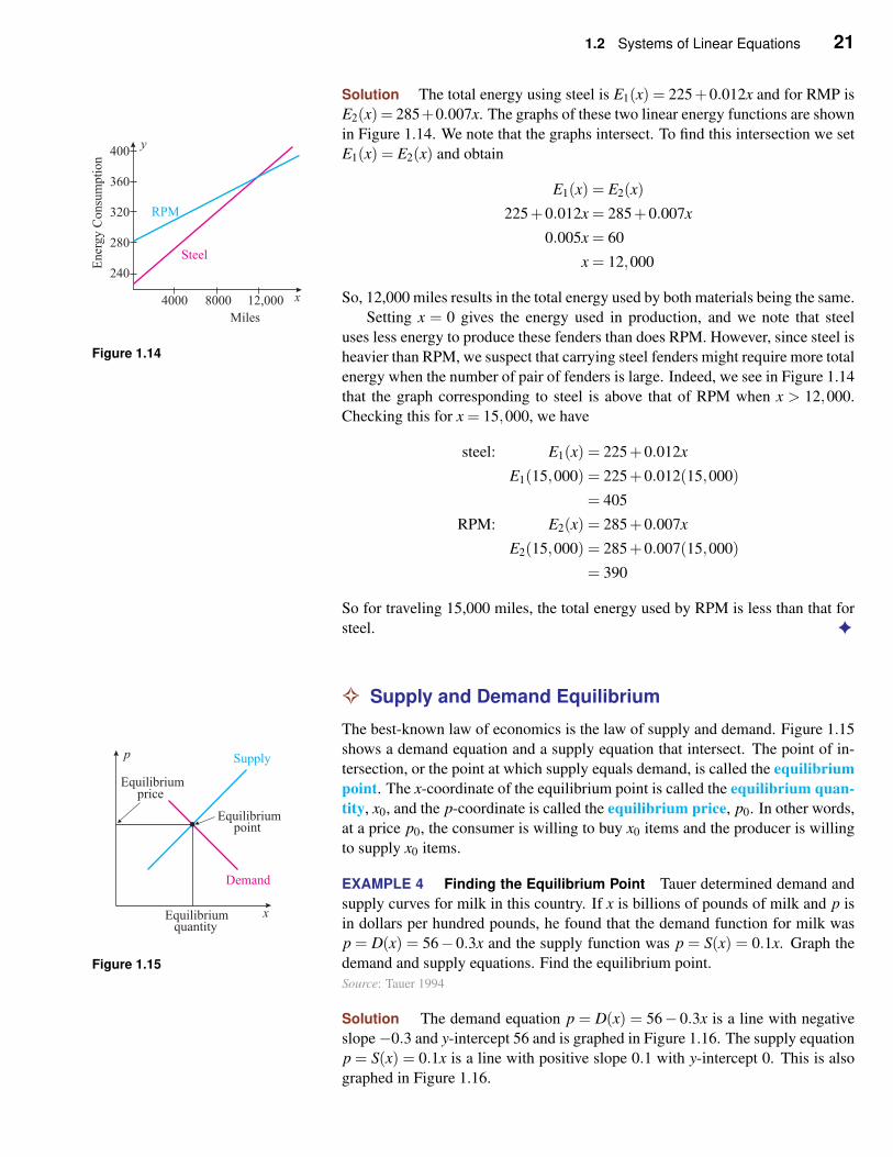
Solution The total energy using steel is E1(x) = 225+0.012x and for RMP is
E2(x) = 285+0.007x. The graphs of these two linear energy functions are shown
in Figure 1.14. We note that the graphs intersect. To find this intersection we set
Figure 1.14
E1(x) = E2(x) and obtain
E1(x) = E2(x)
225+0.012x = 285+0.007x
0.005x = 60
x = 12,000
So, 12,000 miles results in the total energy used by both materials being the same.
Setting x = 0 gives the energy used in production, and we note that steel
uses less energy to produce these fenders than does RPM. However, since steel is
heavier than RPM, we suspect that carrying steel fenders might require more total
energy when the number of pair of fenders is large. Indeed, we see in Figure 1.14
that the graph corresponding to steel is above that of RPM when x > 12,000.
Checking this for x = 15,000, we have
steel: E1(x) = 225+0.012x
E1(15,000) = 225+0.012(15,000)
= 405
RPM: E2(x) = 285+0.007x
E2(15,000) = 285+0.007(15,000)
= 390
So for traveling 15,000 miles, the total energy used by RPM is less than that for
steel. ✦
✧ Supply and Demand Equilibrium
The best-known law of economics is the law of supply and demand. Figure 1.15
shows a demand equation and a supply equation that intersect. The point of in-
tersection, or the point at which supply equals demand, is called the equilibrium
point. The x-coordinate of the equilibrium point is called the equilibrium quan-
tity, x0, and the p-coordinate is called the equilibrium price, p0. In other words,
at a price p0, the consumer is willing to buy x0 items and the producer is willing
to supply x0 items.
Figure 1.15
EXAMPLE 4 Finding the Equilibrium Point Tauer determined demand and
supply curves for milk in this country. If x is billions of pounds of milk and p is
in dollars per hundred pounds, he found that the demand function for milk was
p = D(x) = 56− 0.3x and the supply function was p = S(x) = 0.1x. Graph the
demand and supply equations. Find the equilibrium point.
Source: Tauer 1994
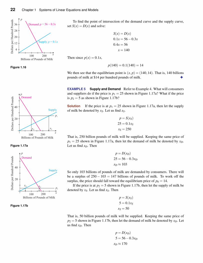
Solution The demand equation p = D(x) = 56− 0.3x is a line with negative
slope−0.3 and y-intercept 56 and is graphed in Figure 1.16. The supply equation
p = S(x) = 0.1x is a line with positive slope 0.1 with y-intercept 0. This is also
graphed in Figure 1.16.
22 Chapter 1 Systems of Linear Equations and Models
To find the point of intersection of the demand curve and the supply curve,
set S(x) = D(x) and solve:
S(x) = D(x)
0.1x = 56−0.3x
0.4x = 56
x = 140
Then since p(x) = 0.1x,
Figure 1.16p(140) = 0.1(140) = 14
We then see that the equilibrium point is (x, p) = (140,14). That is, 140 billions
pounds of milk at $14 per hundred pounds of milk. ✦
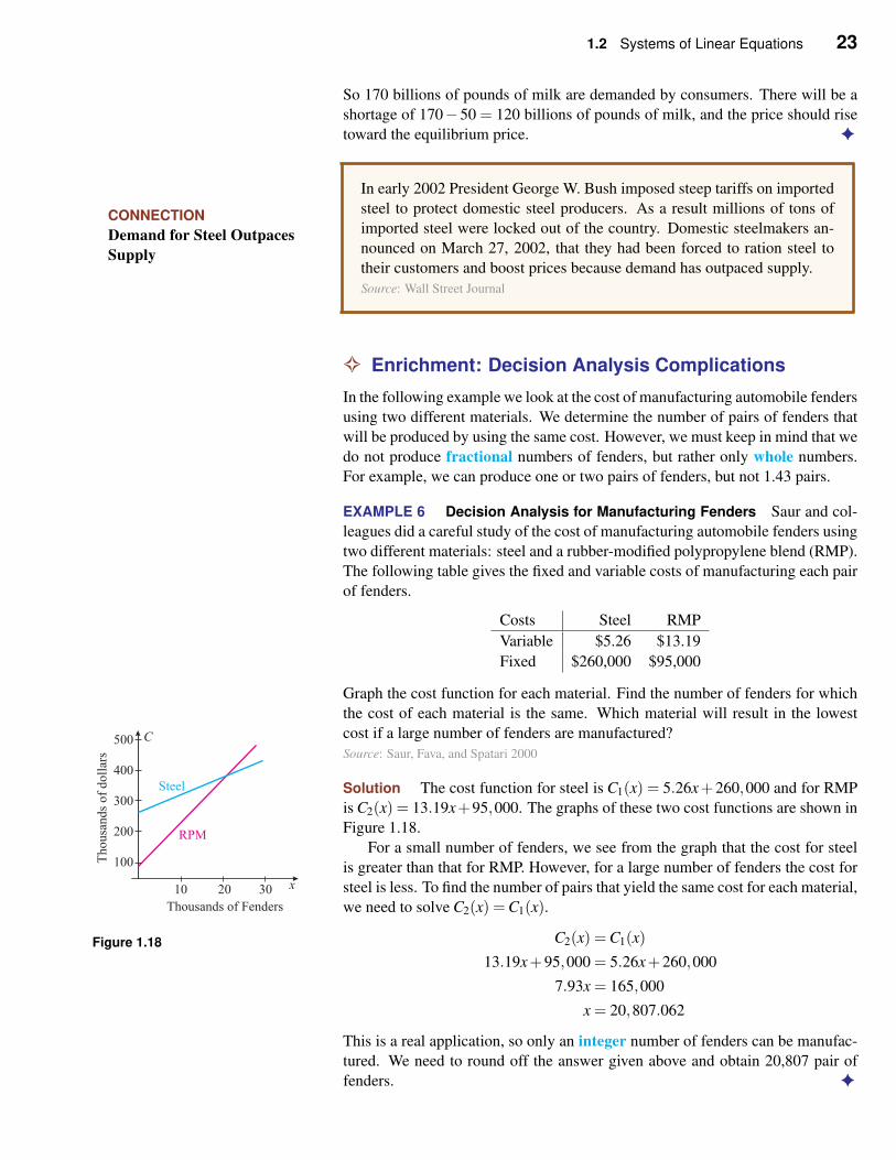
EXAMPLE 5 Supply and Demand Refer to Example 4. What will consumers
and suppliers do if the price is p1 = 25 shown in Figure 1.17a? What if the price
is p2 = 5 as shown in Figure 1.17b?
Solution If the price is at p1 = 25 shown in Figure 1.17a, then let the supply
of milk be denoted by xS. Let us find xS.
Figure 1.17a
p = S(xS)
25 = 0.1xS
xS = 250
That is, 250 billion pounds of milk will be supplied. Keeping the same price of
p1 = 25 shown in Figure 1.17a, then let the demand of milk be denoted by xD.
Let us find xD. Then
p = D(xD)
25 = 56−0.3xD
xD ≈ 103
So only 103 billions of pounds of milk are demanded by consumers. There will
be a surplus of 250− 103 = 147 billions of pounds of milk. To work off the
surplus, the price should fall toward the equilibrium price of p0 = 14.
If the price is at p2 = 5 shown in Figure 1.17b, then let the supply of milk be
denoted by xS. Let us find xS. Then
Figure 1.17b
p = S(xS)
5 = 0.1xS
xS = 50
That is, 50 billion pounds of milk will be supplied. Keeping the same price of
p2 = 5 shown in Figure 1.17b, then let the demand of milk be denoted by xD. Let
us find xD. Then
p = D(xD)
5 = 56−0.3xD
xD ≈ 170
1.2 Systems of Linear Equations 23
So 170 billions of pounds of milk are demanded by consumers. There will be a
shortage of 170−50 = 120 billions of pounds of milk, and the price should rise
toward the equilibrium price. ✦
CONNECTION
Demand for Steel Outpaces
Supply
In early 2002 President George W. Bush imposed steep tariffs on imported
steel to protect domestic steel producers. As a result millions of tons of
imported steel were locked out of the country. Domestic steelmakers an-
nounced on March 27, 2002, that they had been forced to ration steel to
their customers and boost prices because demand has outpaced supply.
Source: Wall Street Journal
✧ Enrichment: Decision Analysis Complications
In the following example we look at the cost of manufacturing automobile fenders
using two different materials. We determine the number of pairs of fenders that
will be produced by using the same cost. However, we must keep in mind that we
do not produce fractional numbers of fenders, but rather only whole numbers.
For example, we can produce one or two pairs of fenders, but not 1.43 pairs.
EXAMPLE 6 Decision Analysis for Manufacturing Fenders Saur and col-
leagues did a careful study of the cost of manufacturing automobile fenders using
two different materials: steel and a rubber-modified polypropylene blend (RMP).
The following table gives the fixed and variable costs of manufacturing each pair
of fenders.
Costs Steel RMP
Variable $5.26 $13.19
Fixed $260,000 $95,000
Graph the cost function for each material. Find the number of fenders for which
the cost of each material is the same. Which material will result in the lowest
cost if a large number of fenders are manufactured?
Source: Saur, Fava, and Spatari 2000
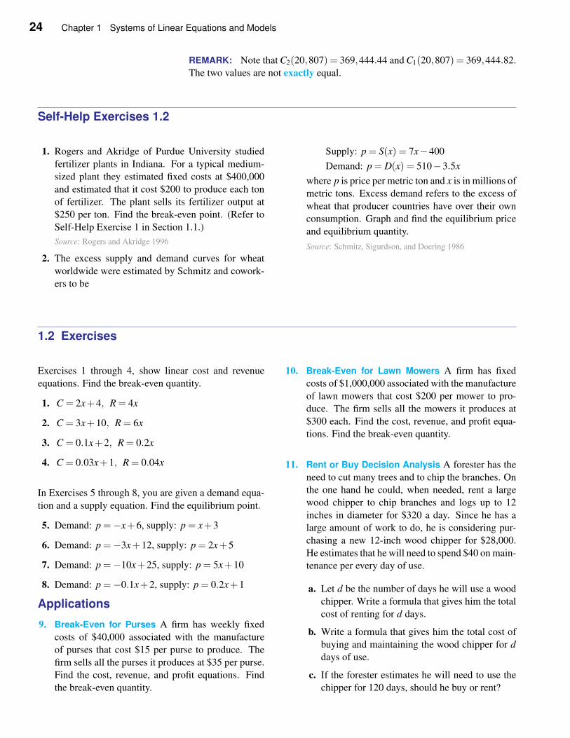
Solution The cost function for steel is C1(x) = 5.26x+260,000 and for RMP
is C2(x) = 13.19x+95,000. The graphs of these two cost functions are shown in
Figure 1.18.
For a small number of fenders, we see from the graph that the cost for steel
is greater than that for RMP. However, for a large number of fenders the cost for
steel is less. To find the number of pairs that yield the same cost for each material,
we need to solve C2(x) =C1(x).
Figure 1.18 C2(x) =C1(x)
13.19x+95,000 = 5.26x+260,000
7.93x = 165,000
x = 20,807.062
This is a real application, so only an integer number of fenders can be manufac-
tured. We need to round off the answer given above and obtain 20,807 pair of
fenders. ✦
24 Chapter 1 Systems of Linear Equations and Models
REMARK: Note that C2(20,807) = 369,444.44 and C1(20,807) = 369,444.82.
The two values are not exactly equal.
Self-Help Exercises 1.2
1. Rogers and Akridge of Purdue University studied
fertilizer plants in Indiana. For a typical medium-
sized plant they estimated fixed costs at $400,000
and estimated that it cost $200 to produce each ton
of fertilizer. The plant sells its fertilizer output at
$250 per ton. Find the break-even point. (Refer to
Self-Help Exercise 1 in Section 1.1.)
Source: Rogers and Akridge 1996
2. The excess supply and demand curves for wheat
worldwide were estimated by Schmitz and cowork-
ers to be
Supply: p = S(x) = 7x−400
Demand: p = D(x) = 510−3.5x
where p is price per metric ton and x is in millions of
metric tons. Excess demand refers to the excess of
wheat that producer countries have over their own
consumption. Graph and find the equilibrium price
and equilibrium quantity.
Source: Schmitz, Sigurdson, and Doering 1986
1.2 Exercises
Exercises 1 through 4, show linear cost and revenue
equations. Find the break-even quantity.
1. C = 2x+4, R = 4x
2. C = 3x+10, R = 6x
3. C = 0.1x+2, R = 0.2x
4. C = 0.03x+1, R = 0.04x
In Exercises 5 through 8, you are given a demand equa-
tion and a supply equation. Find the equilibrium point.
5. Demand: p =−x+6, supply: p = x+3
6. Demand: p =−3x+12, supply: p = 2x+5
7. Demand: p =−10x+25, supply: p = 5x+10
8. Demand: p =−0.1x+2, supply: p = 0.2x+1
Applications
9. Break-Even for Purses A firm has weekly fixed
costs of $40,000 associated with the manufacture
of purses that cost $15 per purse to produce. The
firm sells all the purses it produces at $35 per purse.
Find the cost, revenue, and profit equations. Find
the break-even quantity.
10. Break-Even for Lawn Mowers A firm has fixed
costs of $1,000,000 associated with the manufacture
of lawn mowers that cost $200 per mower to pro-
duce. The firm sells all the mowers it produces at
$300 each. Find the cost, revenue, and profit equa-
tions. Find the break-even quantity.
11. Rent or Buy Decision Analysis A forester has the
need to cut many trees and to chip the branches. On
the one hand he could, when needed, rent a large
wood chipper to chip branches and logs up to 12
inches in diameter for $320 a day. Since he has a
large amount of work to do, he is considering pur-
chasing a new 12-inch wood chipper for $28,000.
He estimates that he will need to spend $40 on main-
tenance per every day of use.
a. Let d be the number of days he will use a wood
chipper. Write a formula that gives him the total
cost of renting for d days.
b. Write a formula that gives him the total cost of
buying and maintaining the wood chipper for d
days of use.
c. If the forester estimates he will need to use the
chipper for 120 days, should he buy or rent?
1.2 Systems of Linear Equations 25
d. Determine the number of days of use before the
forester can save as much money by buying the
chipper as opposed to renting.
12. Decision Analysis for Making Copies At Lincoln
Library there are two ways to pay for copying. You
can pay 5 cents a copy, or you can buy a plastic card
for $5 and then pay 3 cents a copy. Let x be the
number of copies you make. Write an equation for
your costs for each way of paying.
a. How many copies do you need to make before
buying the plastic card is the same as cash?
b. If you wish to make 300 copies, which way of
paying has the least cost?
13. Energy Decision Analysis Many home and busi-
ness owners in northern Ohio can successfully drill
for natural gas on their property. They have the
choice of obtaining natural gas free from their own
gas well or buying the gas from a utility company.
A garden center would need to buy $5000 worth of
gas each year from the local utility company to heat
their greenhouses. They determine that the cost of
drilling a small commercial gas well for the garden
center will be $40,000 and they assume that their
well will need $1000 of maintenance each year.
a. Write a formula that gives the cost of the natural
gas bought from the utility for x years.
b. Write a formula that gives the cost of obtaining
the natural gas from their well over x years.
c. How many years will it be before the cost of gas
from the utility equals the cost of gas from the
well?
CONNECTION: We know an individual living in a
private home in northern Ohio who had a gas and
oil well drilled some years ago. The well yields
both natural gas and oil. Both products go into
a splitter that separates the natural gas and the
oil. The oil goes into a large tank and is sold to
a local utility. The natural gas is used to heat the
home and the excess is fed into the utility company
pipes, where it is measured and purchased by the
utility.
14. Compensation Decision Analysis A salesman for
carpets has been offered two possible compensa-
tion plans. The first offers him a monthly salary
of $2000 plus a royalty of 10% of the total dollar
amount of sales he makes. The second offers him
a monthly salary of $1000 plus a royalty of 20% of
the total dollar amount of sales he makes.
a. Write a formula that gives each compensation
package as a function of the dollar amount x of
sales he makes.
b. Suppose he believes he can sell $15,000 of car-
peting each month. Which compensation pack-
age should he choose?
c. How much carpeting will he sell each month if
he earns the same amount of money with either
compensation package?
15. Truck Rental Decision Analysis A builder needs
to rent a dump truck from Acme Rental for $75 plus
$.40 per mile or the same one from Bell Rental for
$105 plus $.25 per mile. Find a cost function for
using each rental firm.
a. Find the number of miles for which each cost
function will give the same cost.
b. If the builder wants to rent a dump truck to use
for 150 miles, which rental place will cost less?
16. Wood Chipper Rental Decision Analysis A con-
tractor wants to rent a wood chipper from Acme
Rental for a day for $150 plus $10 per hour or from
Bell Rental for a day for $165 plus $7 per hour. Find
a cost function for using each rental firm.
a. Find the number of hours for which each cost
function will give the same cost.
b. If the contractor wants to rent the chipper for 8
hours, which rental place will cost less?
17. Make or Buy Decision A company includes a man-
ual with each piece of software it sells and is try-
ing to decide whether to contract with an outside
supplier to produce it or to produce it in-house.
The lowest bid of any outside supplier is $.75 per
manual. The company estimates that producing the
manuals in-house will require fixed costs of $10,000
and variable costs of $.50 per manual. Find the
number of manuals resulting in the same cost for
contracting with the outside supplier and producing
in-house. If 50,000 manuals are needed, should the
company go with outside supplier or go in-house?
18. Decision Analysis for a Sewing Machine A shirt
manufacturer is considering purchasing a standard
sewing machine for $91,000 and for which it will
cost $2 to sew each shirt. They are also consider-
ing purchasing a more efficient sewing machine for
$100,000 and for which it will cost $1.25 to sew
each shirt. Find a cost function for purchasing and
using each machine.
a. Find the number of shirts for which each cost
function will give the same cost.
26 Chapter 1 Systems of Linear Equations and Models
b. If the manufacturer wishes to sew 10,000 shirts,
which machine should they purchase?
19. Equilibrium Point for Organic Carrots A farmer
will supply 8 bunches of organic carrots to a restau-
rant at a price of $2.50 per bunch. If he can get
$.25 more per bunch, he will supply 10 bunches.
The restaurant’s demand for organic carrot bunches
is given by p = D(x) = −0.1x+ 6, where x is the
number of bunches of organic carrots. What is the
equilibrium point?
20. Equilibrium Point for Cinnamon Rolls A baker
will supply 16 jumbo cinnamon rolls to a cafe at
a price of $1.70 each. If she is offered $1.50,
then she will supply 4 fewer rolls to the cafe. The
cafe’s demand for jumbo cinnamon rolls is given by
p = D(x) = −0.16x+ 7.2. What is the equilibrium
point?
Referenced Applications
21. Break-Even Quantity for Rice Production in Thai-
land Kekhora and McCann estimated a cost func-
tion for the rice production function in Thailand.
They gave the fixed costs per hectare of $75 and the
variable costs per hectare of $371. The revenue per
hectare was given as $573. Suppose the price for
rice went down. What would be the minimum price
to charge per hectare to determine the break-even
quantity?
Source: Kekhora and McCann 2003
22. Break-Even Quantity for Shrimp Production in
Thailand Kekhora and McCann estimated a cost
function for a shrimp production function in Thai-
land. They gave the fixed costs per hectare of $1838
and the variable costs per hectare of $14,183. The
revenue per hectare was given as $26,022. Suppose
the price for shrimp went down. What would be the
revenue to determine the break-even quantity?
Source: Kekhora and McCann 2003
23. Break-Even Quantity for Small Fertilizer Plants
In 1996 Rogers and Akridge of Purdue Univer-
sity studied fertilizer plants in Indiana. For a typ-
ical small-sized plant they estimated fixed costs at
$235,487 and estimated that it cost $206.68 to pro-
duce each ton of fertilizer. The plant sells its fertil-
izer output at $266.67 per ton. Find the break-even
quantity.
Source: Rogers and Akridge 1996
24. Break-Even Quantity for Large Fertilizer Plants
In 1996 Rogers and Akridge of Purdue Univer-
sity studied fertilizer plants in Indiana. For a typ-
ical large-sized plant they estimated fixed costs at
$447,917 and estimated that it cost $209.03 to pro-
duce each ton of fertilizer. The plant sells its fertil-
izer output at $266.67 per ton. Find the break-even
quantity.
Source: Rogers and Akridge 1996
25. Break-Even Quantity on Kansas Beef Cow Farms
Featherstone and coauthors studied 195 Kansas beef
cow farms. The average fixed and variable costs are
in the following table.
Costs per cow
Feed costs $261
Labor costs $82
Utilities and fuel costs $19
Veterinary expenses costs $13
Miscellaneous costs $18
Total variable costs $393
Total fixed costs $13,386
The farm can sell each cow for $470. Find the
break-even quantity.
Source: Featherstone, Langemeier, and Ismet 1997
In Exercises 26 and 27 use the following information.
In the Saur study of fenders mentioned in Exercise 41
of Section 1.1, the amount of energy consumed by each
type of fender was also analyzed. The total energy was
the sum of the energy needed for production plus the en-
ergy consumed by the vehicle used in carrying the fend-
ers. If x is the miles traveled, then the total energy con-
sumption equations for steel, aluminum, and NPN were
as follows:
Steel: E = 225+0.012x
Al: E = 550+0.007x
NPN: E = 565+0.007x
26. Find the number of miles traveled for which the to-
tal energy consumed is the same for steel and NPN
fenders. If 6000 miles is traveled, which material
would use the least energy?
27. Find the number of miles traveled for which the to-
tal energy consumed is the same for steel and alu-
minum fenders. If 5000 miles is traveled, which ma-
terial would use the least energy?
For Exercises 28 and 29 refer to the following informa-
tion. In the Saur study of fenders mentioned in Exam-
ple 3, the amount of CO2 emissions in kg per 2 fenders
of the production and utilization into the air of each type
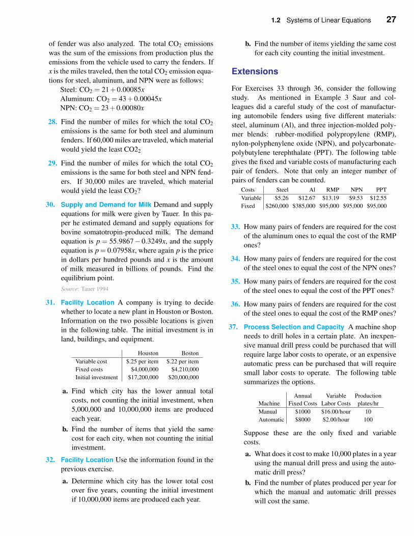
1.2 Systems of Linear Equations 27
of fender was also analyzed. The total CO2 emissions
was the sum of the emissions from production plus the
emissions from the vehicle used to carry the fenders. If
x is the miles traveled, then the total CO2 emission equa-
tions for steel, aluminum, and NPN were as follows:
Steel: CO2 = 21+0.00085x
Aluminum: CO2 = 43+0.00045x
NPN: CO2 = 23+0.00080x
28. Find the number of miles for which the total CO2
emissions is the same for both steel and aluminum
fenders. If 60,000 miles are traveled, which material
would yield the least CO22
29. Find the number of miles for which the total CO2
emissions is the same for both steel and NPN fend-
ers. If 30,000 miles are traveled, which material
would yield the least CO2?
30. Supply and Demand for Milk Demand and supply
equations for milk were given by Tauer. In this pa-
per he estimated demand and supply equations for
bovine somatotropin-produced milk. The demand
equation is p = 55.9867− 0.3249x, and the supply
equation is p = 0.07958x, where again p is the price
in dollars per hundred pounds and x is the amount
of milk measured in billions of pounds. Find the
equilibrium point.
Source: Tauer 1994
31. Facility Location A company is trying to decide
whether to locate a new plant in Houston or Boston.
Information on the two possible locations is given
in the following table. The initial investment is in
land, buildings, and equipment.
Houston Boston
Variable cost $.25 per item $.22 per item
Fixed costs $4,000,000 $4,210,000
Initial investment $17,200,000 $20,000,000
a. Find which city has the lower annual total
costs, not counting the initial investment, when
5,000,000 and 10,000,000 items are produced
each year.
b. Find the number of items that yield the same
cost for each city, when not counting the initial
investment.
32. Facility Location Use the information found in the
previous exercise.
a. Determine which city has the lower total cost
over five years, counting the initial investment
if 10,000,000 items are produced each year.
b. Find the number of items yielding the same cost
for each city counting the initial investment.
Extensions
For Exercises 33 through 36, consider the following
study. As mentioned in Example 3 Saur and col-
leagues did a careful study of the cost of manufactur-
ing automobile fenders using five different materials:
steel, aluminum (Al), and three injection-molded poly-
mer blends: rubber-modified polypropylene (RMP),
nylon-polyphenylene oxide (NPN), and polycarbonate-
polybutylene terephthalate (PPT). The following table
gives the fixed and variable costs of manufacturing each
pair of fenders. Note that only an integer number of
pairs of fenders can be counted.
Costs Steel Al RMP NPN PPT
Variable $5.26 $12.67 $13.19 $9.53 $12.55
Fixed $260,000 $385,000 $95,000 $95,000 $95,000
33. How many pairs of fenders are required for the cost
of the aluminum ones to equal the cost of the RMP
ones?
34. How many pairs of fenders are required for the cost
of the steel ones to equal the cost of the NPN ones?
35. How many pairs of fenders are required for the cost
of the steel ones to equal the cost of the PPT ones?
36. How many pairs of fenders are required for the cost
of the steel ones to equal the cost of the RMP ones?
37. Process Selection and Capacity A machine shop
needs to drill holes in a certain plate. An inexpen-
sive manual drill press could be purchased that will
require large labor costs to operate, or an expensive
automatic press can be purchased that will require
small labor costs to operate. The following table
summarizes the options.
Annual Variable Production
Machine Fixed Costs Labor Costs plates/hr
Manual $1000 $16.00/hour 10
Automatic $8000 $2.00/hour 100
Suppose these are the only fixed and variable
costs.
a. What does it cost to make 10,000 plates in a year
using the manual drill press and using the auto-
matic drill press?
b. Find the number of plates produced per year for
which the manual and automatic drill presses
will cost the same.
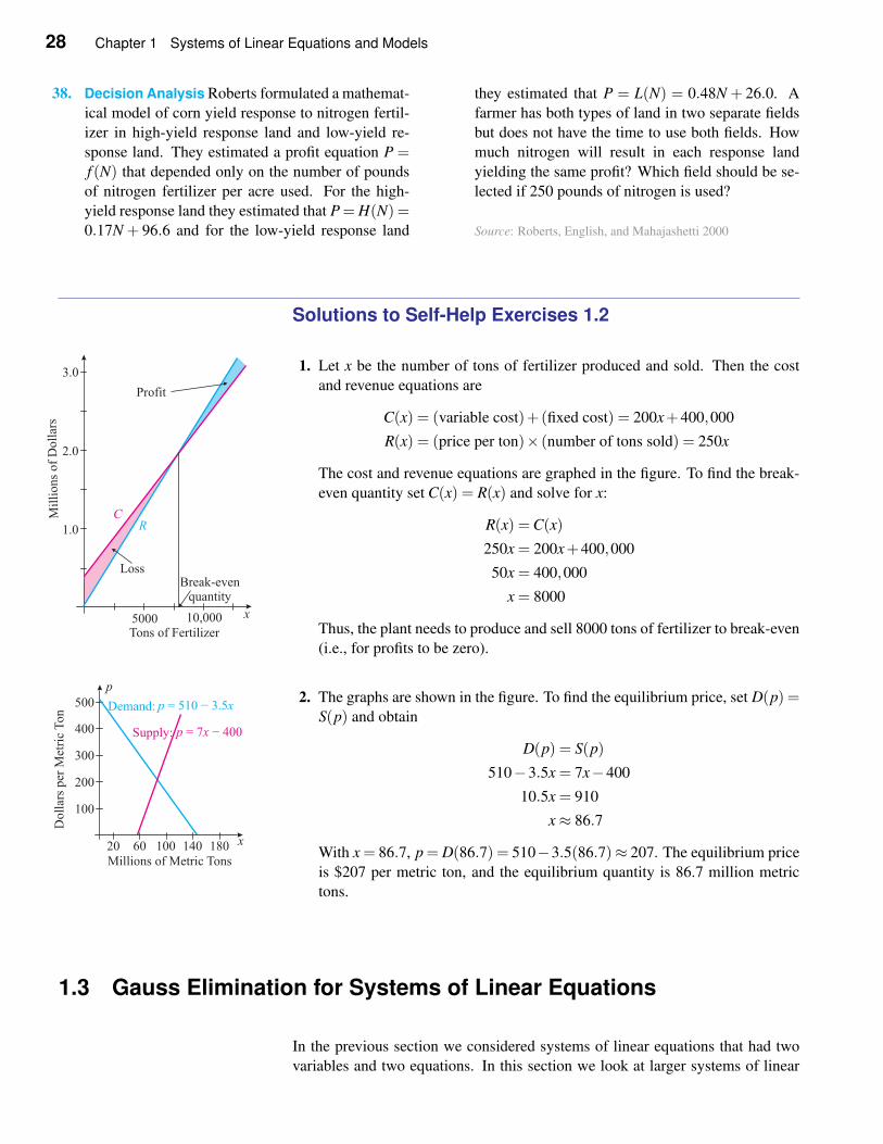
28 Chapter 1 Systems of Linear Equations and Models
38. Decision Analysis Roberts formulated a mathemat-
ical model of corn yield response to nitrogen fertil-
izer in high-yield response land and low-yield re-
sponse land. They estimated a profit equation P =f (N) that depended only on the number of pounds
of nitrogen fertilizer per acre used. For the high-
yield response land they estimated that P = H(N) =0.17N + 96.6 and for the low-yield response land
they estimated that P = L(N) = 0.48N + 26.0. A
farmer has both types of land in two separate fields
but does not have the time to use both fields. How
much nitrogen will result in each response land
yielding the same profit? Which field should be se-
lected if 250 pounds of nitrogen is used?
Source: Roberts, English, and Mahajashetti 2000
Solutions to Self-Help Exercises 1.2
1. Let x be the number of tons of fertilizer produced and sold. Then the cost
and revenue equations are
C(x) = (variable cost)+(fixed cost) = 200x+400,000
R(x) = (price per ton)× (number of tons sold) = 250x
The cost and revenue equations are graphed in the figure. To find the break-
even quantity set C(x) = R(x) and solve for x:
R(x) =C(x)
250x = 200x+400,000
50x = 400,000
x = 8000
Thus, the plant needs to produce and sell 8000 tons of fertilizer to break-even
(i.e., for profits to be zero).
2. The graphs are shown in the figure. To find the equilibrium price, set D(p) =S(p) and obtain
D(p) = S(p)
510−3.5x = 7x−400
10.5x = 910
x≈ 86.7
With x = 86.7, p = D(86.7) = 510−3.5(86.7)≈ 207. The equilibrium price
is $207 per metric ton, and the equilibrium quantity is 86.7 million metric
tons.
1.3 Gauss Elimination for Systems of Linear Equations
In the previous section we considered systems of linear equations that had two
variables and two equations. In this section we look at larger systems of linear
1.3 Gauss Elimination for Systems of Linear Equations 29
equations that have unique solutions. Systems with no solution or non-unique
solutions are covered in the next section. To solve these larger systems we will
develop the method of Gauss elimination, an efficient and systematic manner of
finding the solution to systems of linear equations. For example, consider the
following system of linear equations:
x + 2y + 7z = 14
x − 3y + 2z = 4
2x − y − 3z = −5
Our method is to first eliminate the x variable from all the equations below
the first. Then eliminate the y variable from the equation below the second, and
so forth. After this, we are left with a system like the following:
x + 2y + 7z = 14
y − z = 2
z = 1
We notice that we have found that z = 1. We now use backward substitu-
tion. That is, the value for z substituted into the next to the last equation. We
can solve for the y variable and then substitute the values for y and z into the first
equation and solve for x. In the discussion below we will determine an efficient
and systematical manner of preparing the system for backward substitution.
✧ Creating Systems of Linear Equations
In the first example we examine how to translate English sentences into equa-
tions. Nearly all word problems follow a similar format. First you are given
some information and then you are asked “How much?” or “How many?”. Al-
ways begin your work on a word problem by clearly defining your variables —
they are the answer to the “How much?” or “How many?” question you were
asked. The next step is to take the given information and translate it into an
equation using the variables you defined. A table or diagram is often helpful to
organize the information.
EXAMPLE 1 Document Scheduling An insurance company has two types of
documents to process: contracts and leases. Each contract needs to be examined
for 2 hours by the accountant and 3 hours by the attorney, while each lease needs
to be examined for 4 hours by the accountant and 1 hour by the attorney. If the
accountant has 40 hours and the attorney 30 hours each week to spend working
on these documents, how many documents of each type can they process?
Solution The question asked is “how many documents of each type?”. This
indicates what the unknowns are: the number of contracts and the number of
leases. So letx = the number of contracts
y = the number of leases
Since there are x contracts and the accountant spends 2 hours per week on each of
these, the accountant spends 2x hours per week on contracts. The attorney spends
3x hours per week on contracts. There are y leases and the accountant spends 4
hours per week on each of these, so the accountant spends 4y hours per week on
leases and the attorney spends y hours per week on leases.
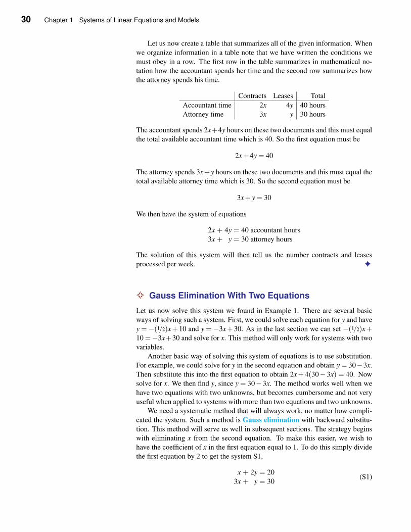
30 Chapter 1 Systems of Linear Equations and Models
Let us now create a table that summarizes all of the given information. When
we organize information in a table note that we have written the conditions we
must obey in a row. The first row in the table summarizes in mathematical no-
tation how the accountant spends her time and the second row summarizes how
the attorney spends his time.
Contracts Leases Total
Accountant time 2x 4y 40 hours
Attorney time 3x y 30 hours
The accountant spends 2x+4y hours on these two documents and this must equal
the total available accountant time which is 40. So the first equation must be
2x+4y = 40
The attorney spends 3x+y hours on these two documents and this must equal the
total available attorney time which is 30. So the second equation must be
3x+ y = 30
We then have the system of equations
2x + 4y = 40 accountant hours
3x + y = 30 attorney hours
The solution of this system will then tell us the number contracts and leases
processed per week. ✦
✧ Gauss Elimination With Two Equations
Let us now solve this system we found in Example 1. There are several basic
ways of solving such a system. First, we could solve each equation for y and have
y = −(1/2)x+ 10 and y = −3x+ 30. As in the last section we can set −(1/2)x+10 =−3x+30 and solve for x. This method will only work for systems with two
variables.
Another basic way of solving this system of equations is to use substitution.
For example, we could solve for y in the second equation and obtain y = 30−3x.
Then substitute this into the first equation to obtain 2x+ 4(30− 3x) = 40. Now
solve for x. We then find y, since y = 30−3x. The method works well when we
have two equations with two unknowns, but becomes cumbersome and not very
useful when applied to systems with more than two equations and two unknowns.
We need a systematic method that will always work, no matter how compli-
cated the system. Such a method is Gauss elimination with backward substitu-
tion. This method will serve us well in subsequent sections. The strategy begins
with eliminating x from the second equation. To make this easier, we wish to
have the coefficient of x in the first equation equal to 1. To do this simply divide
the first equation by 2 to get the system S1,
x + 2y = 20
3x + y = 30(S1)
1.3 Gauss Elimination for Systems of Linear Equations 31
Now we more readily see how to eliminate x from the second equation. We
multiply the first equation by −3, written −3(first), and add this to the second
equation to get a new second equation. We have
−3(first) : −3x − 6y = −60
+(second) : 3x + y = 30
− 5y = −30
This last equation is the new second equation. We now have the system as
x + 2y = 20
− 5y = −30
Notice that we have eliminated the x variable from the second equation. We then
divide the last equation by −5 and obtain
x + 2y = 20
y = 6
We have y = 6. Now substitute this back into the first equation and obtain
x+2y = 20
x+2(6) = 20
x = 20−12 = 8
We then have the solution (x,y) = (8,6). This means that eight of the contracts
documents can be processed and six of the leases.
When we manipulated the equations in Example 1, we followed three basic
rules that allowed us to change the system of equations from one form to another
form with the same solution as the original system. But it was easy to determine
the solution in the new system. For convenience we will denote the first equation
by E1, the second equation by E2, the third equation by E3, and so forth. The
rules that must be followed are below.
Elementary Equation Operations
1. Two equations can be interchanged, Ei↔ E j.
2. An equation may be multiplied by a non-zero constant,
kEi→ Ei.
3. A multiple of one equation may be added to another equation,
Ei + kE j→ Ei.
Gauss elimination is the systematic use of these three allowed operations to
put the system of equations into an easily solved form.
✧ Gauss Elimination
We will now develop Gauss elimination for a system with any number of equa-
tions with any number of unknowns. In this section we continue to restrict our-
selves to examples for which there is a unique solution. We will consider the
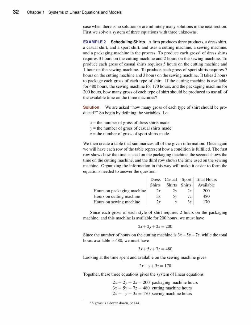
32 Chapter 1 Systems of Linear Equations and Models
case when there is no solution or are infinitely many solutions in the next section.
First we solve a system of three equations with three unknowns.
EXAMPLE 2 Scheduling Shirts A firm produces three products, a dress shirt,
a casual shirt, and a sport shirt, and uses a cutting machine, a sewing machine,
and a packaging machine in the process. To produce each gross⋆ of dress shirts
requires 3 hours on the cutting machine and 2 hours on the sewing machine. To
produce each gross of casual shirts requires 5 hours on the cutting machine and
1 hour on the sewing machine. To produce each gross of sport shirts requires 7
hours on the cutting machine and 3 hours on the sewing machine. It takes 2 hours
to package each gross of each type of shirt. If the cutting machine is available
for 480 hours, the sewing machine for 170 hours, and the packaging machine for
200 hours, how many gross of each type of shirt should be produced to use all of
the available time on the three machines?
Solution We are asked “how many gross of each type of shirt should be pro-
duced?” So begin by defining the variables. Let
x = the number of gross of dress shirts made
y = the number of gross of casual shirts made
z = the number of gross of sport shirts made
We then create a table that summarizes all of the given information. Once again
we will have each row of the table represent how a condition is fulfilled. The first
row shows how the time is used on the packaging machine, the second shows the
time on the cutting machine, and the third row shows the time used on the sewing
machine. Organizing the information in this way will make it easier to form the
equations needed to answer the question.
Dress Casual Sport Total Hours
Shirts Shirts Shirts Available
Hours on packaging machine 2x 2y 2z 200
Hours on cutting machine 3x 5y 7z 480
Hours on sewing machine 2x y 3z 170
Since each gross of each style of shirt requires 2 hours on the packaging
machine, and this machine is available for 200 hours, we must have
2x+2y+2z = 200
Since the number of hours on the cutting machine is 3x+5y+7z, while the total
hours available is 480, we must have
3x+5y+7z = 480
Looking at the time spent and available on the sewing machine gives
2x+ y+3z = 170
Together, these three equations gives the system of linear equations
2x + 2y + 2z = 200 packaging machine hours
3x + 5y + 7z = 480 cutting machine hours
2x + y + 3z = 170 sewing machine hours
⋆A gross is a dozen dozen, or 144.
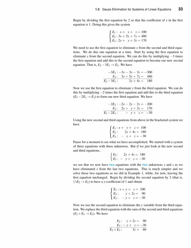
1.3 Gauss Elimination for Systems of Linear Equations 33
Begin by dividing the first equation by 2 so that the coefficient of x in the first
equation is 1. Doing this gives the system
E1 : x + y + z = 100
E2 : 3x + 5y + 7z = 480
E3 : 2x + y + 3z = 170
We need to use the first equation to eliminate x from the second and third equa-
tions. We do this one equation at a time. Start by using the first equation to
eliminate x from the second equation. We can do this by multiplying −3 times
the first equation and add this to the second equation to become our new second
equation. That is, E2−3E1→ E2. We have
−3E1 : −3x − 3y − 3z = −300
E2 : 3x + 5y + 7z = 480
E2−3E1 : 2y + 4z = 180
Now we use the first equation to eliminate x from the third equation. We can do
this by multiplying −2 times the first equation and add this to the third equation
(E3−2E1→ E3) to form our new third equation. We have
−2E1 : −2x − 2y − 2z = −200
E3 : 2x + y + 3z = 170
E3−2E1 : − y + z = −30
Using the new second and third equations from above in the bracketed system we
have
E1 : x + y + z = 100
E2 : 2y + 4z = 180
E3 : − y + z = −30
Pause for a moment to see what we have accomplished. We started with a system
of three equations with three unknowns. But if we just look at the new second
and third equations,{
E2 : 2y + 4z = 180
E3 : − y + z = −30
we see that we now have two equations with the two unknowns y and z as we
have eliminated x from the last two equations. This is much simpler and we
solve these two equations as we did in Example 1, while, for now, leaving the
first equation unchanged. Begin by dividing the second equation by 2 (that is,1/2E2→ E2) to have a y-coefficient of 1 and obtain
E1 : x + y + z = 100
E2 : y + 2z = 90
E3 : − y + z = −30
Now we use the second equation to eliminate the y variable from the third equa-
tion. We replace the third equation with the sum of the second and third equations
(E2 +E3→ E3). We have
E2 : y + 2z = 90
E3 : − y + z = −30
E2 +E3 : 3z = 60
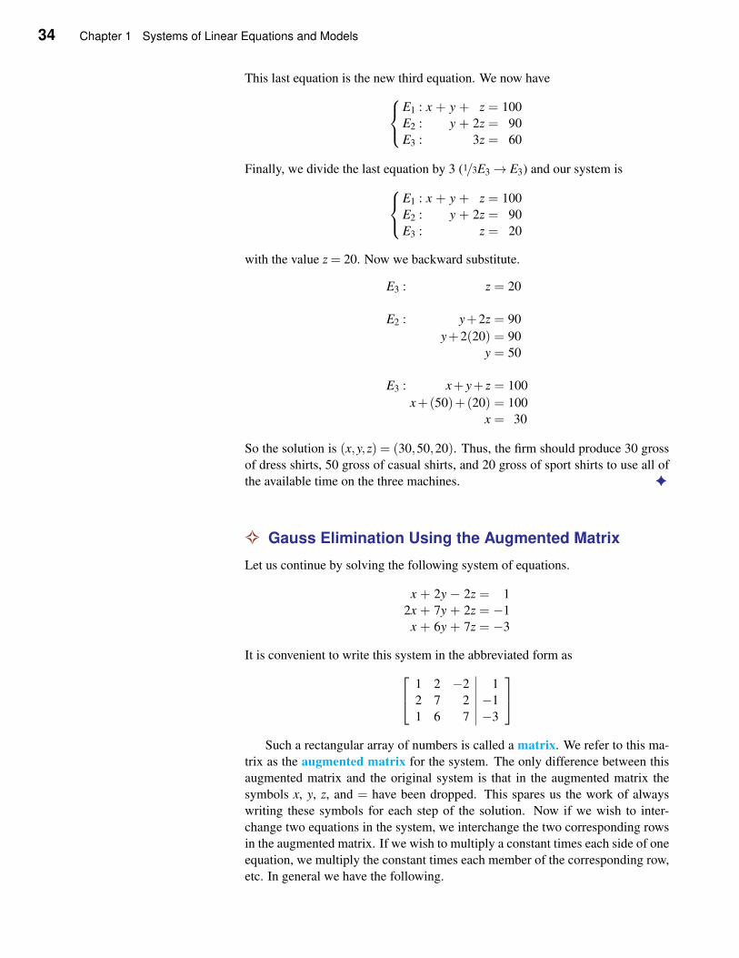
34 Chapter 1 Systems of Linear Equations and Models
This last equation is the new third equation. We now have
E1 : x + y + z = 100
E2 : y + 2z = 90
E3 : 3z = 60
Finally, we divide the last equation by 3 (1/3E3→ E3) and our system is
E1 : x + y + z = 100
E2 : y + 2z = 90
E3 : z = 20
with the value z = 20. Now we backward substitute.
E3 : z = 20
E2 : y+2z = 90
y+2(20) = 90
y = 50
E3 : x+ y+ z = 100
x+(50)+(20) = 100
x = 30
So the solution is (x,y,z) = (30,50,20). Thus, the firm should produce 30 gross
of dress shirts, 50 gross of casual shirts, and 20 gross of sport shirts to use all of
the available time on the three machines. ✦
✧ Gauss Elimination Using the Augmented Matrix
Let us continue by solving the following system of equations.
x + 2y − 2z = 1
2x + 7y + 2z = −1
x + 6y + 7z = −3
It is convenient to write this system in the abbreviated form as
1 2 −2 1
2 7 2 −1
1 6 7 −3
Such a rectangular array of numbers is called a matrix. We refer to this ma-
trix as the augmented matrix for the system. The only difference between this
augmented matrix and the original system is that in the augmented matrix the
symbols x, y, z, and = have been dropped. This spares us the work of always
writing these symbols for each step of the solution. Now if we wish to inter-
change two equations in the system, we interchange the two corresponding rows
in the augmented matrix. If we wish to multiply a constant times each side of one
equation, we multiply the constant times each member of the corresponding row,
etc. In general we have the following.
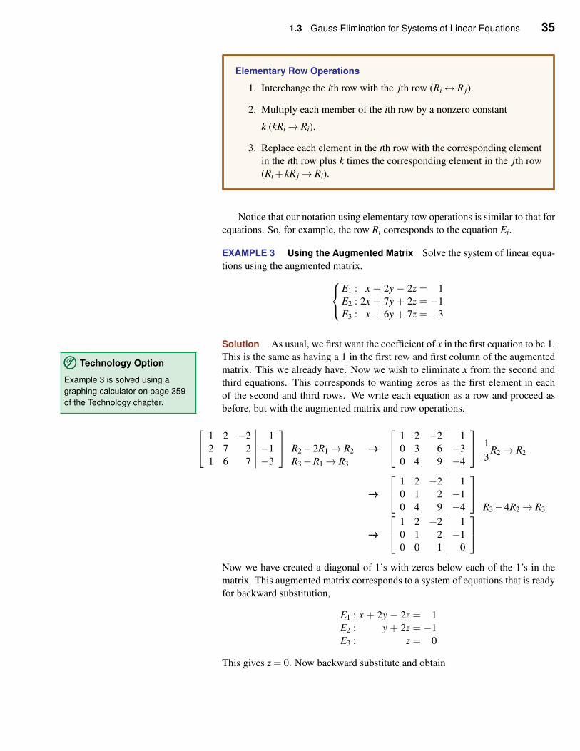
1.3 Gauss Elimination for Systems of Linear Equations 35
Elementary Row Operations
1. Interchange the ith row with the jth row (Ri↔ R j).
2. Multiply each member of the ith row by a nonzero constant
k (kRi→ Ri).
3. Replace each element in the ith row with the corresponding element
in the ith row plus k times the corresponding element in the jth row
(Ri + kR j→ Ri).
Notice that our notation using elementary row operations is similar to that for
equations. So, for example, the row Ri corresponds to the equation Ei.
EXAMPLE 3 Using the Augmented Matrix Solve the system of linear equa-
tions using the augmented matrix.
E1 : x + 2y − 2z = 1
E2 : 2x + 7y + 2z = −1
E3 : x + 6y + 7z = −3
Solution As usual, we first want the coefficient of x in the first equation to be 1.
This is the same as having a 1 in the first row and first column of the augmented
matrix. This we already have. Now we wish to eliminate x from the second and
third equations. This corresponds to wanting zeros as the first element in each
TTT©©© Technology Option
Example 3 is solved using a
graphing calculator on page 359
of the Technology chapter.of the second and third rows. We write each equation as a row and proceed as
before, but with the augmented matrix and row operations.
1 2 −2 1
2 7 2 −1
1 6 7 −3
R2−2R1→ R2
R3−R1→ R3
→→→
1 2 −2 1
0 3 6 −3
0 4 9 −4
1
3R2→ R2
→→→
1 2 −2 1
0 1 2 −1
0 4 9 −4
R3−4R2→ R3
→→→
1 2 −2 1
0 1 2 −1
0 0 1 0
Now we have created a diagonal of 1’s with zeros below each of the 1’s in the
matrix. This augmented matrix corresponds to a system of equations that is ready
for backward substitution,
E1 : x + 2y − 2z = 1
E2 : y + 2z = −1
E3 : z = 0
This gives z = 0. Now backward substitute and obtain
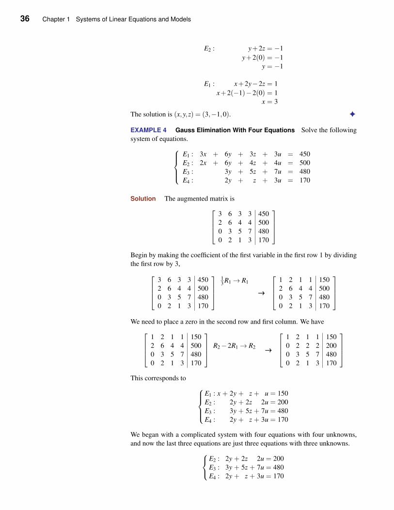
36 Chapter 1 Systems of Linear Equations and Models
E2 : y+2z = −1
y+2(0) = −1
y = −1
E1 : x+2y−2z = 1
x+2(−1)−2(0) = 1
x = 3
The solution is (x,y,z) = (3,−1,0). ✦
EXAMPLE 4 Gauss Elimination With Four Equations Solve the following
system of equations.
E1 : 3x + 6y + 3z + 3u = 450
E2 : 2x + 6y + 4z + 4u = 500
E3 : 3y + 5z + 7u = 480
E4 : 2y + z + 3u = 170
Solution The augmented matrix is
3 6 3 3 450
2 6 4 4 500
0 3 5 7 480
0 2 1 3 170
Begin by making the coefficient of the first variable in the first row 1 by dividing
the first row by 3,
3 6 3 3 450
2 6 4 4 500
0 3 5 7 480
0 2 1 3 170
13 R1→ R1
→→→
1 2 1 1 150
2 6 4 4 500
0 3 5 7 480
0 2 1 3 170
We need to place a zero in the second row and first column. We have
1 2 1 1 150
2 6 4 4 500
0 3 5 7 480
0 2 1 3 170
R2−2R1→ R2 →→→
1 2 1 1 150
0 2 2 2 200
0 3 5 7 480
0 2 1 3 170
This corresponds to
E1 : x + 2y + z + u = 150
E2 : 2y + 2z 2u = 200
E3 : 3y + 5z + 7u = 480
E4 : 2y + z + 3u = 170
We began with a complicated system with four equations with four unknowns,
and now the last three equations are just three equations with three unknowns.
E2 : 2y + 2z 2u = 200
E3 : 3y + 5z + 7u = 480
E4 : 2y + z + 3u = 170
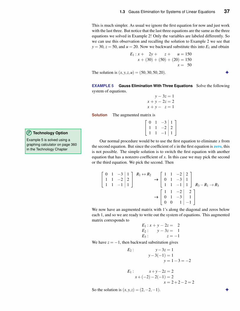
1.3 Gauss Elimination for Systems of Linear Equations 37
This is much simpler. As usual we ignore the first equation for now and just work
with the last three. But notice that the last three equations are the same as the three
equations we solved in Example 2! Only the variables are labeled differently. So
we can use this observation and recalling the solution to Example 2 we see that
y = 30, z = 50, and u = 20. Now we backward substitute this into E1 and obtain
E1 : x + 2y + z + u = 150
x + (30) + (50) + (20) = 150
x = 50
The solution is (x,y,z,u) = (50,30,50,20). ✦
EXAMPLE 5 Gauss Elimination With Three Equations Solve the following
system of equations.y − 3z = 1
x + y − 2z = 2
x + y − z = 1
Solution The augmented matrix is
0 1 −3 1
1 1 −2 2
1 1 −1 1
Our normal procedure would be to use the first equation to eliminate x from
TTT©©© Technology Option
Example 5 is solved using a
graphing calculator on page 360
in the Technology Chapterthe second equation. But since the coefficient of x in the first equation is zero, this
is not possible. The simple solution is to switch the first equation with another
equation that has a nonzero coefficient of x. In this case we may pick the second
or the third equation. We pick the second. Then
0 1 −3 1
1 1 −2 2
1 1 −1 1
R1↔ R2
→→→
1 1 −2 2
0 1 −3 1
1 1 −1 1
R3−R1→ R3
→→→
1 1 −2 2
0 1 −3 1
0 0 1 −1
We now have an augmented matrix with 1’s along the diagonal and zeros below
each 1, and so we are ready to write out the system of equations. This augmented
matrix corresponds toE1 : x + y − 2z = 2
E2 : y − 3z = 1
E3 : z = −1
We have z =−1, then backward substitution gives
E2 : y−3z = 1
y−3(−1) = 1
y = 1−3 =−2
E1 : x+ y−2z = 2
x+(−2)−2(−1) = 2
x = 2+2−2 = 2
So the solution is (x,y,z) = (2,−2,−1). ✦
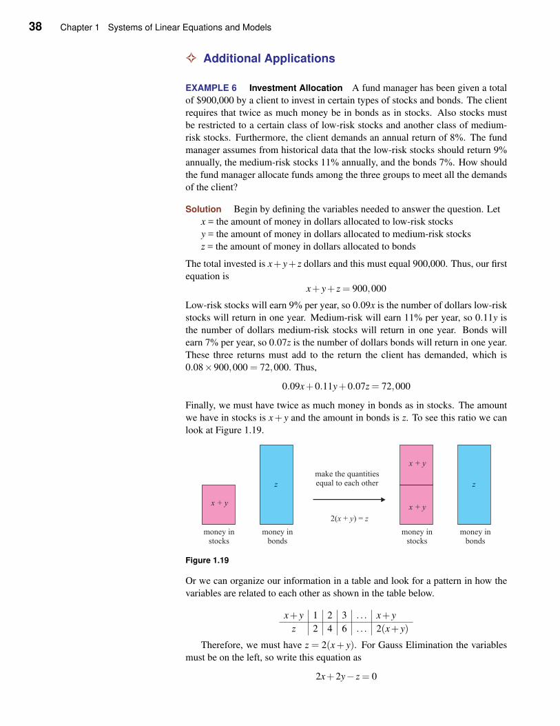
38 Chapter 1 Systems of Linear Equations and Models
✧ Additional Applications
EXAMPLE 6 Investment Allocation A fund manager has been given a total
of $900,000 by a client to invest in certain types of stocks and bonds. The client
requires that twice as much money be in bonds as in stocks. Also stocks must
be restricted to a certain class of low-risk stocks and another class of medium-
risk stocks. Furthermore, the client demands an annual return of 8%. The fund
manager assumes from historical data that the low-risk stocks should return 9%
annually, the medium-risk stocks 11% annually, and the bonds 7%. How should
the fund manager allocate funds among the three groups to meet all the demands
of the client?
Solution Begin by defining the variables needed to answer the question. Let
x = the amount of money in dollars allocated to low-risk stocks
y = the amount of money in dollars allocated to medium-risk stocks
z = the amount of money in dollars allocated to bonds
The total invested is x+y+ z dollars and this must equal 900,000. Thus, our first
equation is
x+ y+ z = 900,000
Low-risk stocks will earn 9% per year, so 0.09x is the number of dollars low-risk
stocks will return in one year. Medium-risk will earn 11% per year, so 0.11y is
the number of dollars medium-risk stocks will return in one year. Bonds will
earn 7% per year, so 0.07z is the number of dollars bonds will return in one year.
These three returns must add to the return the client has demanded, which is
0.08×900,000 = 72,000. Thus,
0.09x+0.11y+0.07z = 72,000
Finally, we must have twice as much money in bonds as in stocks. The amount
we have in stocks is x+ y and the amount in bonds is z. To see this ratio we can
look at Figure 1.19.
Figure 1.19
Or we can organize our information in a table and look for a pattern in how the
variables are related to each other as shown in the table below.
x+ y 1 2 3 . . . x+ y
z 2 4 6 . . . 2(x+ y)
Therefore, we must have z = 2(x+ y). For Gauss Elimination the variables
must be on the left, so write this equation as
2x+2y− z = 0
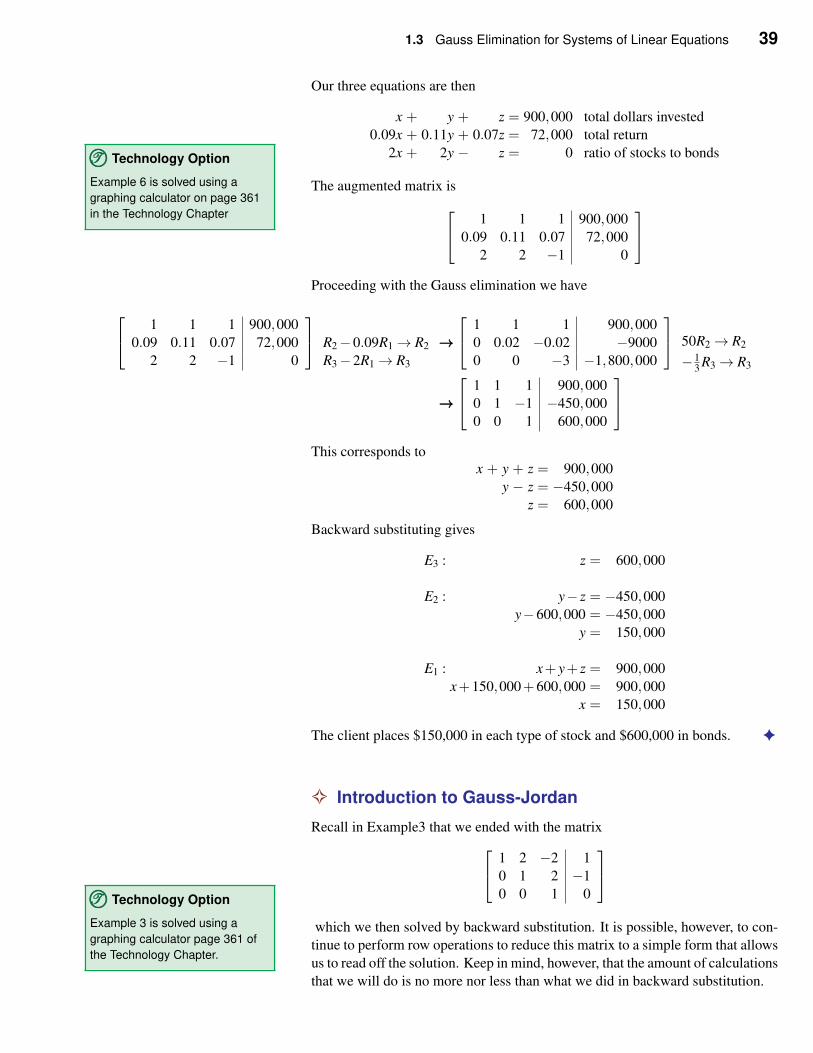
1.3 Gauss Elimination for Systems of Linear Equations 39
Our three equations are then
x + y + z = 900,000 total dollars invested
0.09x + 0.11y + 0.07z = 72,000 total return
2x + 2y − z = 0 ratio of stocks to bonds
The augmented matrix is
TTT©©© Technology Option
Example 6 is solved using a
graphing calculator on page 361
in the Technology Chapter
1 1 1 900,000
0.09 0.11 0.07 72,000
2 2 −1 0
Proceeding with the Gauss elimination we have
1 1 1 900,000
0.09 0.11 0.07 72,000
2 2 −1 0
R2−0.09R1→ R2
R3−2R1→ R3
→→→
1 1 1 900,000
0 0.02 −0.02 −9000
0 0 −3 −1,800,000
50R2→ R2
− 13 R3→ R3
→→→
1 1 1 900,000
0 1 −1 −450,000
0 0 1 600,000
This corresponds tox + y + z = 900,000
y − z = −450,000
z = 600,000
Backward substituting gives
E3 : z = 600,000
E2 : y− z = −450,000
y−600,000 = −450,000
y = 150,000
E1 : x+ y+ z = 900,000
x+150,000+600,000 = 900,000
x = 150,000
The client places $150,000 in each type of stock and $600,000 in bonds. ✦
✧ Introduction to Gauss-Jordan
Recall in Example3 that we ended with the matrix
1 2 −2 1
0 1 2 −1
0 0 1 0
which we then solved by backward substitution. It is possible, however, to con-
TTT©©© Technology Option
Example 3 is solved using a
graphing calculator page 361 of
the Technology Chapter.tinue to perform row operations to reduce this matrix to a simple form that allows
us to read off the solution. Keep in mind, however, that the amount of calculations
that we will do is no more nor less than what we did in backward substitution.
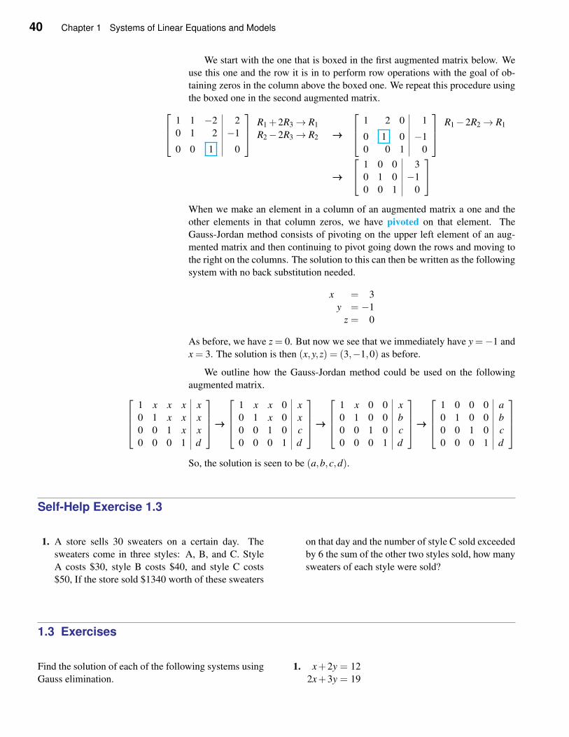
40 Chapter 1 Systems of Linear Equations and Models
We start with the one that is boxed in the first augmented matrix below. We
use this one and the row it is in to perform row operations with the goal of ob-
taining zeros in the column above the boxed one. We repeat this procedure using
the boxed one in the second augmented matrix.
1 1 −2 2
0 1 2 −1
0 0 1 0
R1 +2R3→ R1
R2−2R3→ R2 →→→
1 2 0 1
0 1 0 −1
0 0 1 0
R1−2R2→ R1
→→→
1 0 0 3
0 1 0 −1
0 0 1 0
When we make an element in a column of an augmented matrix a one and the
other elements in that column zeros, we have pivoted on that element. The
Gauss-Jordan method consists of pivoting on the upper left element of an aug-
mented matrix and then continuing to pivot going down the rows and moving to
the right on the columns. The solution to this can then be written as the following
system with no back substitution needed.
x = 3
y = −1
z = 0
As before, we have z = 0. But now we see that we immediately have y =−1 and
x = 3. The solution is then (x,y,z) = (3,−1,0) as before.
We outline how the Gauss-Jordan method could be used on the following
augmented matrix.
1 x x x x
0 1 x x x
0 0 1 x x
0 0 0 1 d
→→→
1 x x 0 x
0 1 x 0 x
0 0 1 0 c
0 0 0 1 d
→→→
1 x 0 0 x
0 1 0 0 b
0 0 1 0 c
0 0 0 1 d
→→→
1 0 0 0 a
0 1 0 0 b
0 0 1 0 c
0 0 0 1 d
So, the solution is seen to be (a,b,c,d).
Self-Help Exercise 1.3
1. A store sells 30 sweaters on a certain day. The
sweaters come in three styles: A, B, and C. Style
A costs $30, style B costs $40, and style C costs
$50, If the store sold $1340 worth of these sweaters
on that day and the number of style C sold exceeded
by 6 the sum of the other two styles sold, how many
sweaters of each style were sold?
1.3 Exercises
Find the solution of each of the following systems using
Gauss elimination.
1. x+2y = 12
2x+3y = 19
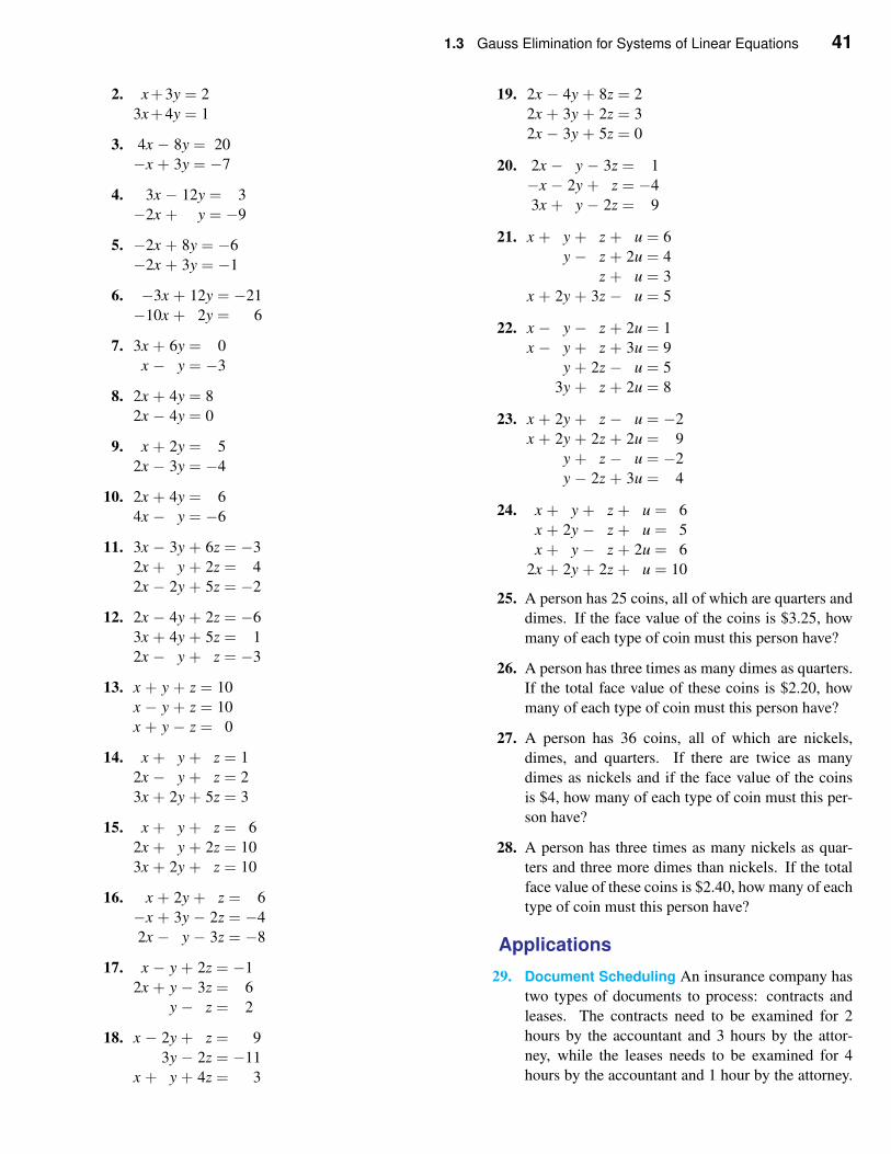
1.3 Gauss Elimination for Systems of Linear Equations 41
2. x+3y = 2
3x+4y = 1
3. 4x − 8y = 20
−x + 3y = −7
4. 3x − 12y = 3
−2x + y = −9
5. −2x + 8y = −6
−2x + 3y = −1
6. −3x + 12y = −21
−10x + 2y = 6
7. 3x + 6y = 0
x − y = −3
8. 2x + 4y = 8
2x − 4y = 0
9. x + 2y = 5
2x − 3y = −4
10. 2x + 4y = 6
4x − y = −6
11. 3x − 3y + 6z = −3
2x + y + 2z = 4
2x − 2y + 5z = −2
12. 2x − 4y + 2z = −6
3x + 4y + 5z = 1
2x − y + z = −3
13. x + y + z = 10
x − y + z = 10
x + y − z = 0
14. x + y + z = 1
2x − y + z = 2
3x + 2y + 5z = 3
15. x + y + z = 6
2x + y + 2z = 10
3x + 2y + z = 10
16. x + 2y + z = 6
−x + 3y − 2z = −4
2x − y − 3z = −8
17. x − y + 2z = −1
2x + y − 3z = 6
y − z = 2
18. x − 2y + z = 9
3y − 2z = −11
x + y + 4z = 3
19. 2x − 4y + 8z = 2
2x + 3y + 2z = 3
2x − 3y + 5z = 0
20. 2x − y − 3z = 1
−x − 2y + z = −4
3x + y − 2z = 9
21. x + y + z + u = 6
y − z + 2u = 4
z + u = 3
x + 2y + 3z − u = 5
22. x − y − z + 2u = 1
x − y + z + 3u = 9
y + 2z − u = 5
3y + z + 2u = 8
23. x + 2y + z − u = −2
x + 2y + 2z + 2u = 9
y + z − u = −2
y − 2z + 3u = 4
24. x + y + z + u = 6
x + 2y − z + u = 5
x + y − z + 2u = 6
2x + 2y + 2z + u = 10
25. A person has 25 coins, all of which are quarters and
dimes. If the face value of the coins is $3.25, how
many of each type of coin must this person have?
26. A person has three times as many dimes as quarters.
If the total face value of these coins is $2.20, how
many of each type of coin must this person have?
27. A person has 36 coins, all of which are nickels,
dimes, and quarters. If there are twice as many
dimes as nickels and if the face value of the coins
is $4, how many of each type of coin must this per-
son have?
28. A person has three times as many nickels as quar-
ters and three more dimes than nickels. If the total
face value of these coins is $2.40, how many of each
type of coin must this person have?
Applications
29. Document Scheduling An insurance company has
two types of documents to process: contracts and
leases. The contracts need to be examined for 2
hours by the accountant and 3 hours by the attor-
ney, while the leases needs to be examined for 4
hours by the accountant and 1 hour by the attorney.
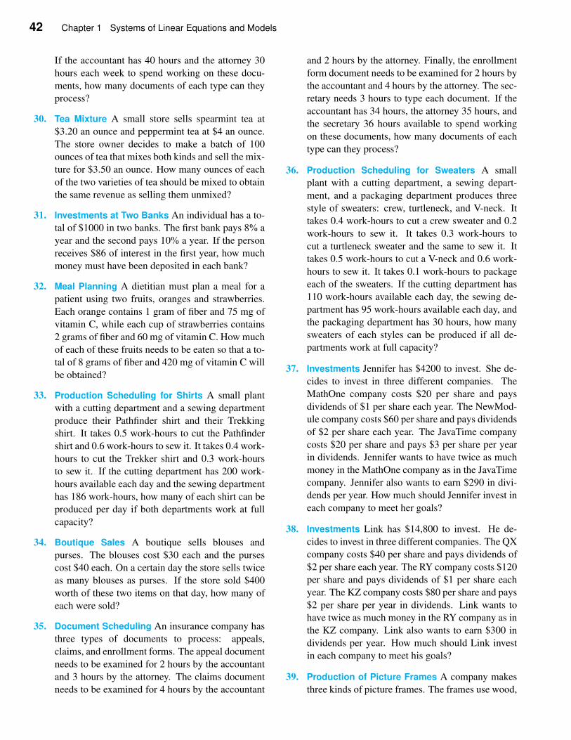
42 Chapter 1 Systems of Linear Equations and Models
If the accountant has 40 hours and the attorney 30
hours each week to spend working on these docu-
ments, how many documents of each type can they
process?
30. Tea Mixture A small store sells spearmint tea at
$3.20 an ounce and peppermint tea at $4 an ounce.
The store owner decides to make a batch of 100
ounces of tea that mixes both kinds and sell the mix-
ture for $3.50 an ounce. How many ounces of each
of the two varieties of tea should be mixed to obtain
the same revenue as selling them unmixed?
31. Investments at Two Banks An individual has a to-
tal of $1000 in two banks. The first bank pays 8% a
year and the second pays 10% a year. If the person
receives $86 of interest in the first year, how much
money must have been deposited in each bank?
32. Meal Planning A dietitian must plan a meal for a
patient using two fruits, oranges and strawberries.
Each orange contains 1 gram of fiber and 75 mg of
vitamin C, while each cup of strawberries contains
2 grams of fiber and 60 mg of vitamin C. How much
of each of these fruits needs to be eaten so that a to-
tal of 8 grams of fiber and 420 mg of vitamin C will
be obtained?
33. Production Scheduling for Shirts A small plant
with a cutting department and a sewing department
produce their Pathfinder shirt and their Trekking
shirt. It takes 0.5 work-hours to cut the Pathfinder
shirt and 0.6 work-hours to sew it. It takes 0.4 work-
hours to cut the Trekker shirt and 0.3 work-hours
to sew it. If the cutting department has 200 work-
hours available each day and the sewing department
has 186 work-hours, how many of each shirt can be
produced per day if both departments work at full
capacity?
34. Boutique Sales A boutique sells blouses and
purses. The blouses cost $30 each and the purses
cost $40 each. On a certain day the store sells twice
as many blouses as purses. If the store sold $400
worth of these two items on that day, how many of
each were sold?
35. Document Scheduling An insurance company has
three types of documents to process: appeals,
claims, and enrollment forms. The appeal document
needs to be examined for 2 hours by the accountant
and 3 hours by the attorney. The claims document
needs to be examined for 4 hours by the accountant
and 2 hours by the attorney. Finally, the enrollment
form document needs to be examined for 2 hours by
the accountant and 4 hours by the attorney. The sec-
retary needs 3 hours to type each document. If the
accountant has 34 hours, the attorney 35 hours, and
the secretary 36 hours available to spend working
on these documents, how many documents of each
type can they process?
36. Production Scheduling for Sweaters A small
plant with a cutting department, a sewing depart-
ment, and a packaging department produces three
style of sweaters: crew, turtleneck, and V-neck. It
takes 0.4 work-hours to cut a crew sweater and 0.2
work-hours to sew it. It takes 0.3 work-hours to
cut a turtleneck sweater and the same to sew it. It
takes 0.5 work-hours to cut a V-neck and 0.6 work-
hours to sew it. It takes 0.1 work-hours to package
each of the sweaters. If the cutting department has
110 work-hours available each day, the sewing de-
partment has 95 work-hours available each day, and
the packaging department has 30 hours, how many
sweaters of each styles can be produced if all de-
partments work at full capacity?
37. Investments Jennifer has $4200 to invest. She de-
cides to invest in three different companies. The
MathOne company costs $20 per share and pays
dividends of $1 per share each year. The NewMod-
ule company costs $60 per share and pays dividends
of $2 per share each year. The JavaTime company
costs $20 per share and pays $3 per share per year
in dividends. Jennifer wants to have twice as much
money in the MathOne company as in the JavaTime
company. Jennifer also wants to earn $290 in divi-
dends per year. How much should Jennifer invest in
each company to meet her goals?
38. Investments Link has $14,800 to invest. He de-
cides to invest in three different companies. The QX
company costs $40 per share and pays dividends of
$2 per share each year. The RY company costs $120
per share and pays dividends of $1 per share each
year. The KZ company costs $80 per share and pays
$2 per share per year in dividends. Link wants to
have twice as much money in the RY company as in
the KZ company. Link also wants to earn $300 in
dividends per year. How much should Link invest
in each company to meet his goals?
39. Production of Picture Frames A company makes
three kinds of picture frames. The frames use wood,
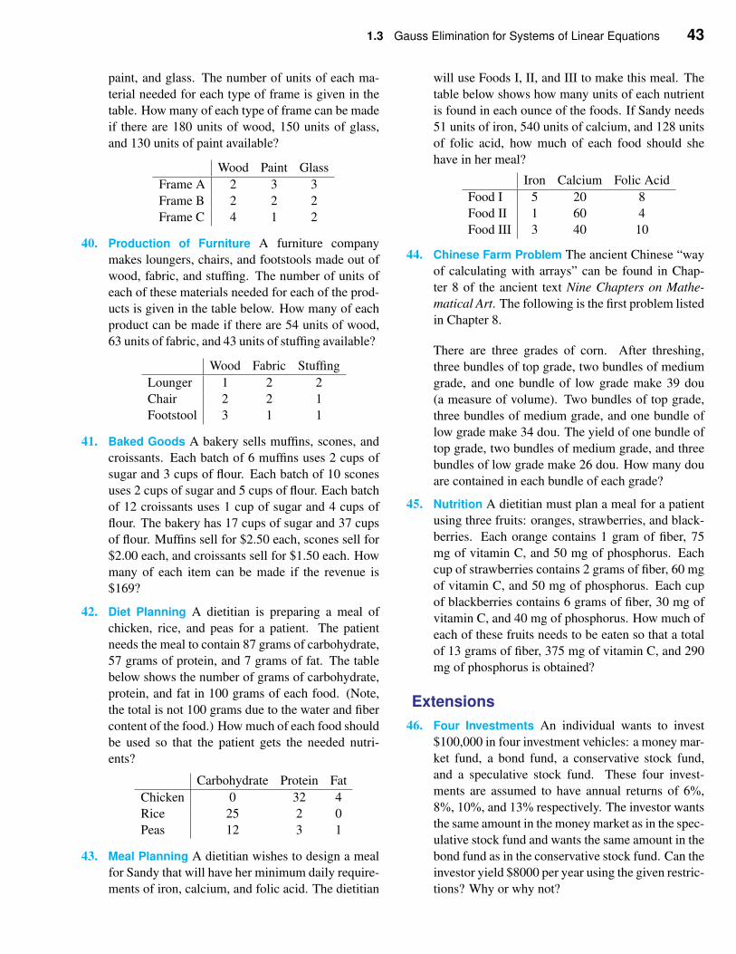
1.3 Gauss Elimination for Systems of Linear Equations 43
paint, and glass. The number of units of each ma-
terial needed for each type of frame is given in the
table. How many of each type of frame can be made
if there are 180 units of wood, 150 units of glass,
and 130 units of paint available?
Wood Paint Glass
Frame A 2 3 3
Frame B 2 2 2
Frame C 4 1 2
40. Production of Furniture A furniture company
makes loungers, chairs, and footstools made out of
wood, fabric, and stuffing. The number of units of
each of these materials needed for each of the prod-
ucts is given in the table below. How many of each
product can be made if there are 54 units of wood,
63 units of fabric, and 43 units of stuffing available?
Wood Fabric Stuffing
Lounger 1 2 2
Chair 2 2 1
Footstool 3 1 1
41. Baked Goods A bakery sells muffins, scones, and
croissants. Each batch of 6 muffins uses 2 cups of
sugar and 3 cups of flour. Each batch of 10 scones
uses 2 cups of sugar and 5 cups of flour. Each batch
of 12 croissants uses 1 cup of sugar and 4 cups of
flour. The bakery has 17 cups of sugar and 37 cups
of flour. Muffins sell for $2.50 each, scones sell for
$2.00 each, and croissants sell for $1.50 each. How
many of each item can be made if the revenue is
$169?
42. Diet Planning A dietitian is preparing a meal of
chicken, rice, and peas for a patient. The patient
needs the meal to contain 87 grams of carbohydrate,
57 grams of protein, and 7 grams of fat. The table
below shows the number of grams of carbohydrate,
protein, and fat in 100 grams of each food. (Note,
the total is not 100 grams due to the water and fiber
content of the food.) How much of each food should
be used so that the patient gets the needed nutri-
ents?
Carbohydrate Protein Fat
Chicken 0 32 4
Rice 25 2 0
Peas 12 3 1
43. Meal Planning A dietitian wishes to design a meal
for Sandy that will have her minimum daily require-
ments of iron, calcium, and folic acid. The dietitian
will use Foods I, II, and III to make this meal. The
table below shows how many units of each nutrient
is found in each ounce of the foods. If Sandy needs
51 units of iron, 540 units of calcium, and 128 units
of folic acid, how much of each food should she
have in her meal?
Iron Calcium Folic Acid
Food I 5 20 8
Food II 1 60 4
Food III 3 40 10
44. Chinese Farm Problem The ancient Chinese “way
of calculating with arrays” can be found in Chap-
ter 8 of the ancient text Nine Chapters on Mathe-
matical Art. The following is the first problem listed
in Chapter 8.
There are three grades of corn. After threshing,
three bundles of top grade, two bundles of medium
grade, and one bundle of low grade make 39 dou
(a measure of volume). Two bundles of top grade,
three bundles of medium grade, and one bundle of
low grade make 34 dou. The yield of one bundle of
top grade, two bundles of medium grade, and three
bundles of low grade make 26 dou. How many dou
are contained in each bundle of each grade?
45. Nutrition A dietitian must plan a meal for a patient
using three fruits: oranges, strawberries, and black-
berries. Each orange contains 1 gram of fiber, 75
mg of vitamin C, and 50 mg of phosphorus. Each
cup of strawberries contains 2 grams of fiber, 60 mg
of vitamin C, and 50 mg of phosphorus. Each cup
of blackberries contains 6 grams of fiber, 30 mg of
vitamin C, and 40 mg of phosphorus. How much of
each of these fruits needs to be eaten so that a total
of 13 grams of fiber, 375 mg of vitamin C, and 290
mg of phosphorus is obtained?
Extensions
46. Four Investments An individual wants to invest
$100,000 in four investment vehicles: a money mar-
ket fund, a bond fund, a conservative stock fund,
and a speculative stock fund. These four invest-
ments are assumed to have annual returns of 6%,
8%, 10%, and 13% respectively. The investor wants
the same amount in the money market as in the spec-
ulative stock fund and wants the same amount in the
bond fund as in the conservative stock fund. Can the
investor yield $8000 per year using the given restric-
tions? Why or why not?
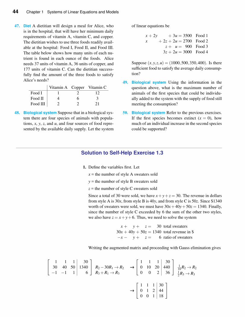
44 Chapter 1 Systems of Linear Equations and Models
47. Diet A dietitian will design a meal for Alice, who
is in the hospital, that will have her minimum daily
requirements of vitamin A, vitamin C, and copper.
The dietitian wishes to use three foods readily avail-
able at the hospital: Food I, Food II, and Food III.
The table below shows how many units of each nu-
trient is found in each ounce of the foods. Alice
needs 37 units of vitamin A, 36 units of copper, and
177 units of vitamin C. Can the dietitian success-
fully find the amount of the three foods to satisfy
Alice’s needs?
Vitamin A Copper Vitamin C
Food I 1 2 12
Food II 4 6 3
Food III 2 2 21
48. Biological system Suppose that in a biological sys-
tem there are four species of animals with popula-
tions, x, y, z, and u, and four sources of food repre-
sented by the available daily supply. Let the system
of linear equations be
x + 2y + 3u = 3500 Food 1
x + 2z + 2u = 2700 Food 2
z + u = 900 Food 3
3z + 2u = 3000 Food 4
Suppose (x,y,z,u) = (1000,500,350,400). Is there
sufficient food to satisfy the average daily consump-
tion?
49. Biological system Using the information in the
question above, what is the maximum number of
animals of the first species that could be individu-
ally added to the system with the supply of food still
meeting the consumption?
50. Biological system Refer to the previous exercises.
If the first species becomes extinct (x = 0), how
much of an individual increase in the second species
could be supported?
Solution to Self-Help Exercise 1.3
1. Define the variables first. Let
x = the number of style A sweaters sold
y = the number of style B sweaters sold
z = the number of style C sweaters sold
Since a total of 30 were sold, we have x+ y+ z = 30. The revenue in dollars
from style A is 30x, from style B is 40y, and from style C is 50z. Since $1340
worth of sweaters were sold, we must have 30x+40y+50z = 1340. Finally,
since the number of style C exceeded by 6 the sum of the other two styles,
we also have z = x+ y+6. Thus, we need to solve the system
x + y + z = 30 total sweaters
30x + 40y + 50z = 1340 total revenue in $
−x − y + z = 6 ratio of sweaters
Writing the augmented matrix and proceeding with Gauss elimination gives
1 1 1 30
30 40 50 1340
−1 −1 1 6
R2−30R1→ R2
R3 +R1→ R3
→→→
1 1 1 30
0 10 20 440
0 0 2 36
110 R2→ R2
12 R3→ R3
→→→
1 1 1 30
0 1 2 44
0 0 1 18
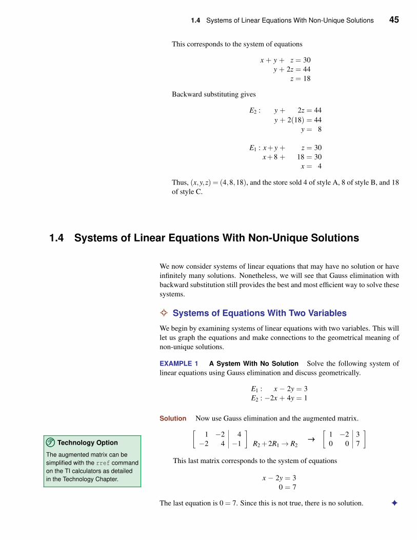
1.4 Systems of Linear Equations With Non-Unique Solutions 45
This corresponds to the system of equations
x + y + z = 30
y + 2z = 44
z = 18
Backward substituting gives
E2 : y + 2z = 44
y + 2(18) = 44
y = 8
E1 : x+ y + z = 30
x+8 + 18 = 30
x = 4
Thus, (x,y,z) = (4,8,18), and the store sold 4 of style A, 8 of style B, and 18
of style C.
1.4 Systems of Linear Equations With Non-Unique Solutions
We now consider systems of linear equations that may have no solution or have
infinitely many solutions. Nonetheless, we will see that Gauss elimination with
backward substitution still provides the best and most efficient way to solve these
systems.
✧ Systems of Equations With Two Variables
We begin by examining systems of linear equations with two variables. This will
let us graph the equations and make connections to the geometrical meaning of
non-unique solutions.
EXAMPLE 1 A System With No Solution Solve the following system of
linear equations using Gauss elimination and discuss geometrically.
E1 : x − 2y = 3
E2 : −2x + 4y = 1
Solution Now use Gauss elimination and the augmented matrix.
[1 −2 4
−2 4 −1
]
R2 +2R1→ R2→→→
[1 −2 3
0 0 7
]
This last matrix corresponds to the system of equations
TTT©©© Technology Option
The augmented matrix can be
simplified with the rref command
on the TI calculators as detailed
in the Technology Chapter. x − 2y = 3
0 = 7
The last equation is 0 = 7. Since this is not true, there is no solution. ✦
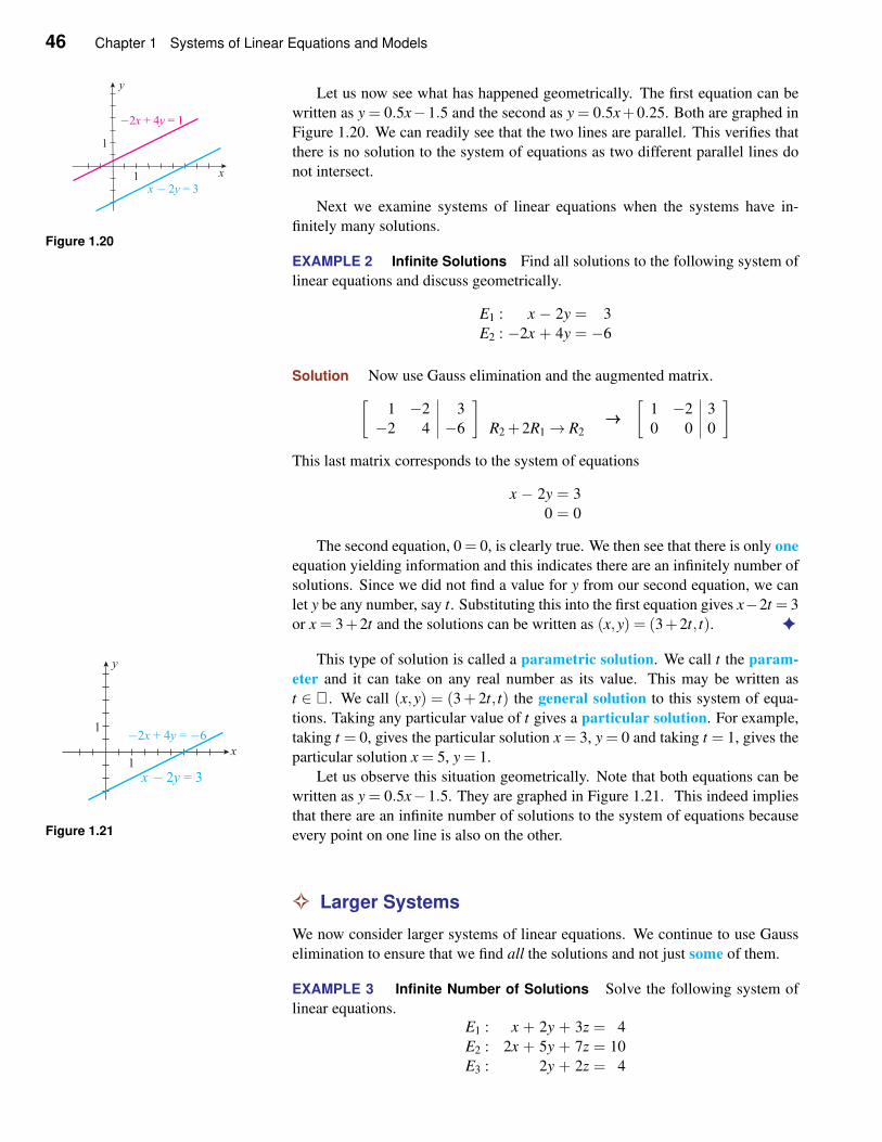
46 Chapter 1 Systems of Linear Equations and Models
Let us now see what has happened geometrically. The first equation can be
written as y = 0.5x−1.5 and the second as y = 0.5x+0.25. Both are graphed in
Figure 1.20. We can readily see that the two lines are parallel. This verifies that
there is no solution to the system of equations as two different parallel lines do
not intersect.
Figure 1.20
Next we examine systems of linear equations when the systems have in-
finitely many solutions.
EXAMPLE 2 Infinite Solutions Find all solutions to the following system of
linear equations and discuss geometrically.
E1 : x − 2y = 3
E2 : −2x + 4y = −6
Solution Now use Gauss elimination and the augmented matrix.
[1 −2 3
−2 4 −6
]
R2 +2R1→ R2→→→
[1 −2 3
0 0 0
]
This last matrix corresponds to the system of equations
x − 2y = 3
0 = 0
The second equation, 0 = 0, is clearly true. We then see that there is only one
equation yielding information and this indicates there are an infinitely number of
solutions. Since we did not find a value for y from our second equation, we can
let y be any number, say t. Substituting this into the first equation gives x−2t = 3
or x = 3+2t and the solutions can be written as (x,y) = (3+2t, t). ✦
This type of solution is called a parametric solution. We call t the param-
eter and it can take on any real number as its value. This may be written as
t ∈ ℜ. We call (x,y) = (3+ 2t, t) the general solution to this system of equa-
tions. Taking any particular value of t gives a particular solution. For example,
taking t = 0, gives the particular solution x = 3, y = 0 and taking t = 1, gives the
particular solution x = 5, y = 1.
Let us observe this situation geometrically. Note that both equations can be
written as y = 0.5x−1.5. They are graphed in Figure 1.21. This indeed implies
Figure 1.21that there are an infinite number of solutions to the system of equations because
every point on one line is also on the other.
✧ Larger Systems
We now consider larger systems of linear equations. We continue to use Gauss
elimination to ensure that we find all the solutions and not just some of them.
EXAMPLE 3 Infinite Number of Solutions Solve the following system of
linear equations.E1 : x + 2y + 3z = 4
E2 : 2x + 5y + 7z = 10
E3 : 2y + 2z = 4
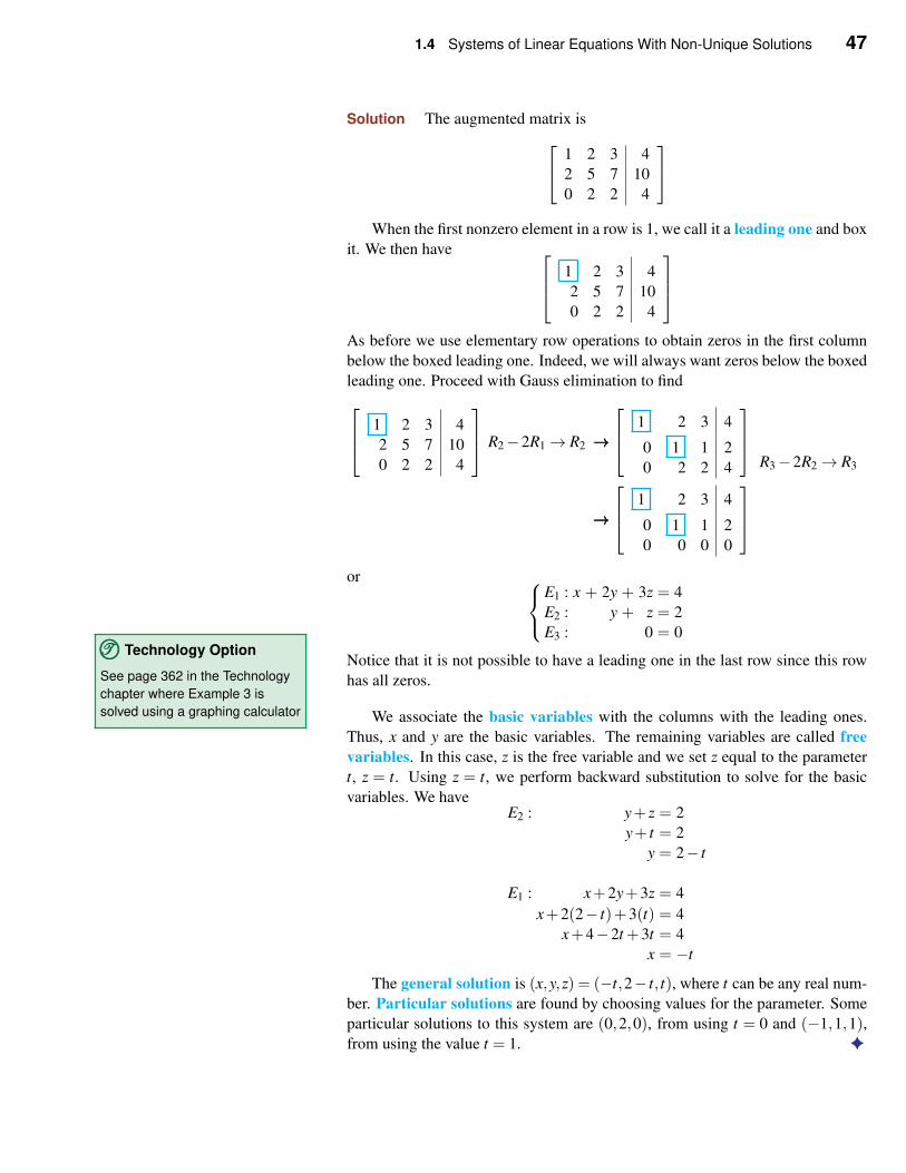
1.4 Systems of Linear Equations With Non-Unique Solutions 47
Solution The augmented matrix is
1 2 3 4
2 5 7 10
0 2 2 4
When the first nonzero element in a row is 1, we call it a leading one and box
it. We then have
1 2 3 4
2 5 7 10
0 2 2 4
As before we use elementary row operations to obtain zeros in the first column
below the boxed leading one. Indeed, we will always want zeros below the boxed
leading one. Proceed with Gauss elimination to find
1 2 3 4
2 5 7 10
0 2 2 4
R2−2R1→ R2 →→→
1 2 3 4
0 1 1 2
0 2 2 4
R3−2R2→ R3
→→→
1 2 3 4
0 1 1 2
0 0 0 0
or
E1 : x + 2y + 3z = 4
E2 : y + z = 2
E3 : 0 = 0
Notice that it is not possible to have a leading one in the last row since this row
has all zeros.
TTT©©© Technology Option
See page 362 in the Technology
chapter where Example 3 is
solved using a graphing calculator We associate the basic variables with the columns with the leading ones.
Thus, x and y are the basic variables. The remaining variables are called free
variables. In this case, z is the free variable and we set z equal to the parameter
t, z = t. Using z = t, we perform backward substitution to solve for the basic
variables. We haveE2 : y+ z = 2
y+ t = 2
y = 2− t
E1 : x+2y+3z = 4
x+2(2− t)+3(t) = 4
x+4−2t +3t = 4
x = −t
The general solution is (x,y,z) = (−t,2− t, t), where t can be any real num-
ber. Particular solutions are found by choosing values for the parameter. Some
particular solutions to this system are (0,2,0), from using t = 0 and (−1,1,1),from using the value t = 1. ✦
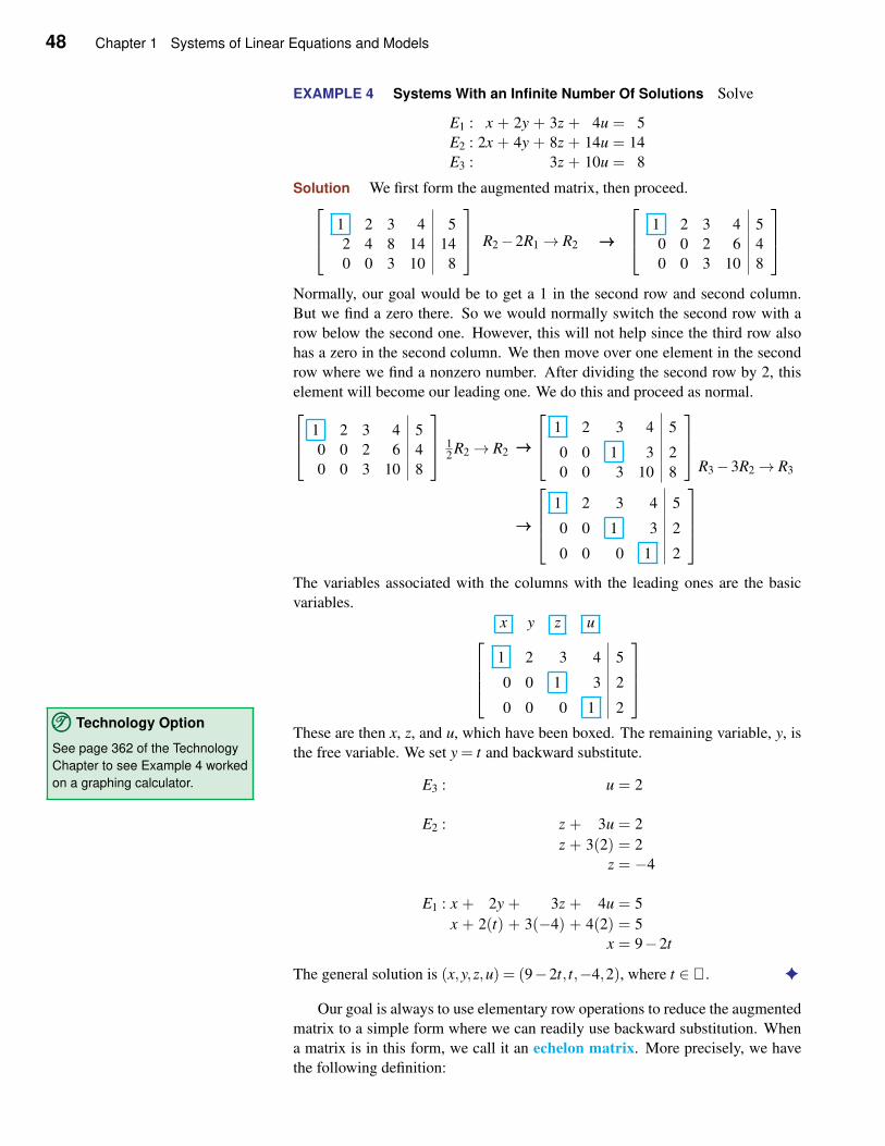
48 Chapter 1 Systems of Linear Equations and Models
EXAMPLE 4 Systems With an Infinite Number Of Solutions Solve
E1 : x + 2y + 3z + 4u = 5
E2 : 2x + 4y + 8z + 14u = 14
E3 : 3z + 10u = 8
Solution We first form the augmented matrix, then proceed.
1 2 3 4 5
2 4 8 14 14
0 0 3 10 8
R2−2R1→ R2 →→→
1 2 3 4 5
0 0 2 6 4
0 0 3 10 8
Normally, our goal would be to get a 1 in the second row and second column.
But we find a zero there. So we would normally switch the second row with a
row below the second one. However, this will not help since the third row also
has a zero in the second column. We then move over one element in the second
row where we find a nonzero number. After dividing the second row by 2, this
element will become our leading one. We do this and proceed as normal.
1 2 3 4 5
0 0 2 6 4
0 0 3 10 8
12 R2→ R2 →→→
1 2 3 4 5
0 0 1 3 2
0 0 3 10 8
R3−3R2→ R3
→→→
1 2 3 4 5
0 0 1 3 2
0 0 0 1 2
The variables associated with the columns with the leading ones are the basic
variables.
x y z u
1 2 3 4 5
0 0 1 3 2
0 0 0 1 2
These are then x, z, and u, which have been boxed. The remaining variable, y, is
the free variable. We set y = t and backward substitute.
TTT©©© Technology Option
See page 362 of the Technology
Chapter to see Example 4 worked
on a graphing calculator. E3 : u = 2
E2 : z + 3u = 2
z + 3(2) = 2
z = −4
E1 : x + 2y + 3z + 4u = 5
x + 2(t) + 3(−4) + 4(2) = 5
x = 9−2t
The general solution is (x,y,z,u) = (9−2t, t,−4,2), where t ∈ℜ. ✦
Our goal is always to use elementary row operations to reduce the augmented
matrix to a simple form where we can readily use backward substitution. When
a matrix is in this form, we call it an echelon matrix. More precisely, we have
the following definition:
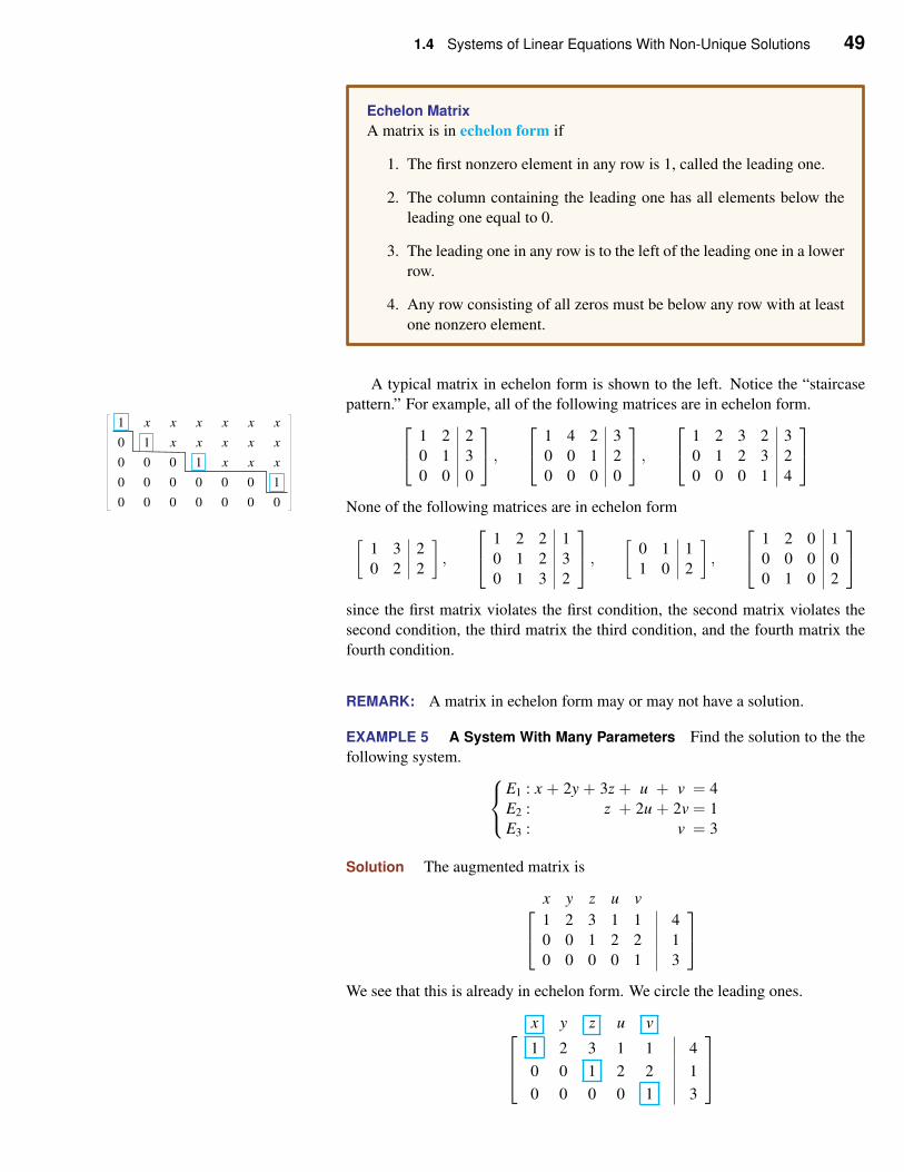
1.4 Systems of Linear Equations With Non-Unique Solutions 49
Echelon Matrix
A matrix is in echelon form if
1. The first nonzero element in any row is 1, called the leading one.
2. The column containing the leading one has all elements below the
leading one equal to 0.
3. The leading one in any row is to the left of the leading one in a lower
row.
4. Any row consisting of all zeros must be below any row with at least
one nonzero element.
A typical matrix in echelon form is shown to the left. Notice the “staircase
pattern.” For example, all of the following matrices are in echelon form.
1 2 2
0 1 3
0 0 0
,
1 4 2 3
0 0 1 2
0 0 0 0
,
1 2 3 2 3
0 1 2 3 2
0 0 0 1 4
None of the following matrices are in echelon form
1
0 1
0 0 0 1
0 0 0 0 0 0 1
0 0 0 0 0 0 0
x x x x x x
x x x x x
x x x
[1 3 2
0 2 2
]
,
1 2 2 1
0 1 2 3
0 1 3 2
,
[0 1 1
1 0 2
]
,
1 2 0 1
0 0 0 0
0 1 0 2
since the first matrix violates the first condition, the second matrix violates the
second condition, the third matrix the third condition, and the fourth matrix the
fourth condition.
REMARK: A matrix in echelon form may or may not have a solution.
EXAMPLE 5 A System With Many Parameters Find the solution to the the
following system.
E1 : x + 2y + 3z + u + v = 4
E2 : z + 2u + 2v = 1
E3 : v = 3
Solution The augmented matrix is
x y z u v
1 2 3 1 1 4
0 0 1 2 2 1
0 0 0 0 1 3
We see that this is already in echelon form. We circle the leading ones.
x y z u v
1 2 3 1 1 4
0 0 1 2 2 1
0 0 0 0 1 3
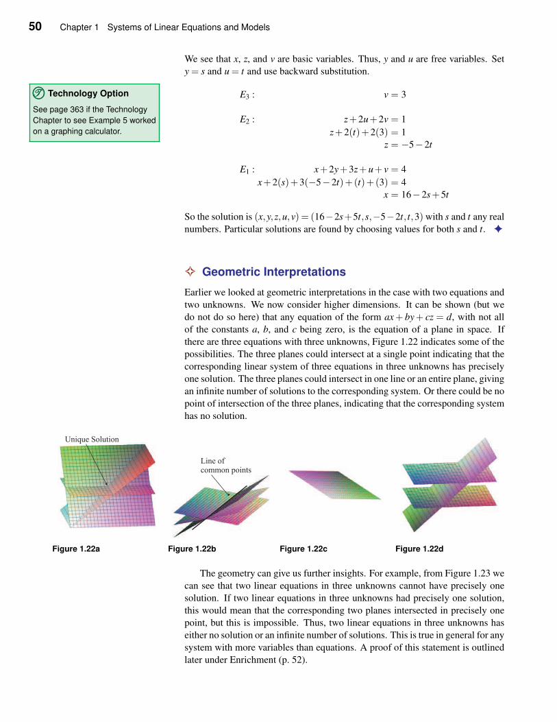
50 Chapter 1 Systems of Linear Equations and Models
We see that x, z, and v are basic variables. Thus, y and u are free variables. Set
y = s and u = t and use backward substitution.
TTT©©© Technology Option
See page 363 if the Technology
Chapter to see Example 5 worked
on a graphing calculator.
E3 : v = 3
E2 : z+2u+2v = 1
z+2(t)+2(3) = 1
z = −5−2t
E1 : x+2y+3z+u+ v = 4
x+2(s)+3(−5−2t)+(t)+(3) = 4
x = 16−2s+5t
So the solution is (x,y,z,u,v) = (16−2s+5t,s,−5−2t, t,3) with s and t any real
numbers. Particular solutions are found by choosing values for both s and t. ✦
✧ Geometric Interpretations
Earlier we looked at geometric interpretations in the case with two equations and
two unknowns. We now consider higher dimensions. It can be shown (but we
do not do so here) that any equation of the form ax+ by+ cz = d, with not all
of the constants a, b, and c being zero, is the equation of a plane in space. If
there are three equations with three unknowns, Figure 1.22 indicates some of the
possibilities. The three planes could intersect at a single point indicating that the
corresponding linear system of three equations in three unknowns has precisely
one solution. The three planes could intersect in one line or an entire plane, giving
an infinite number of solutions to the corresponding system. Or there could be no
point of intersection of the three planes, indicating that the corresponding system
has no solution.
Unique Solution
Figure 1.22a
Line ofcommon points
Figure 1.22b Figure 1.22c Figure 1.22d
The geometry can give us further insights. For example, from Figure 1.23 we
can see that two linear equations in three unknowns cannot have precisely one
solution. If two linear equations in three unknowns had precisely one solution,
this would mean that the corresponding two planes intersected in precisely one
point, but this is impossible. Thus, two linear equations in three unknowns has
either no solution or an infinite number of solutions. This is true in general for any
system with more variables than equations. A proof of this statement is outlined
later under Enrichment (p. 52).
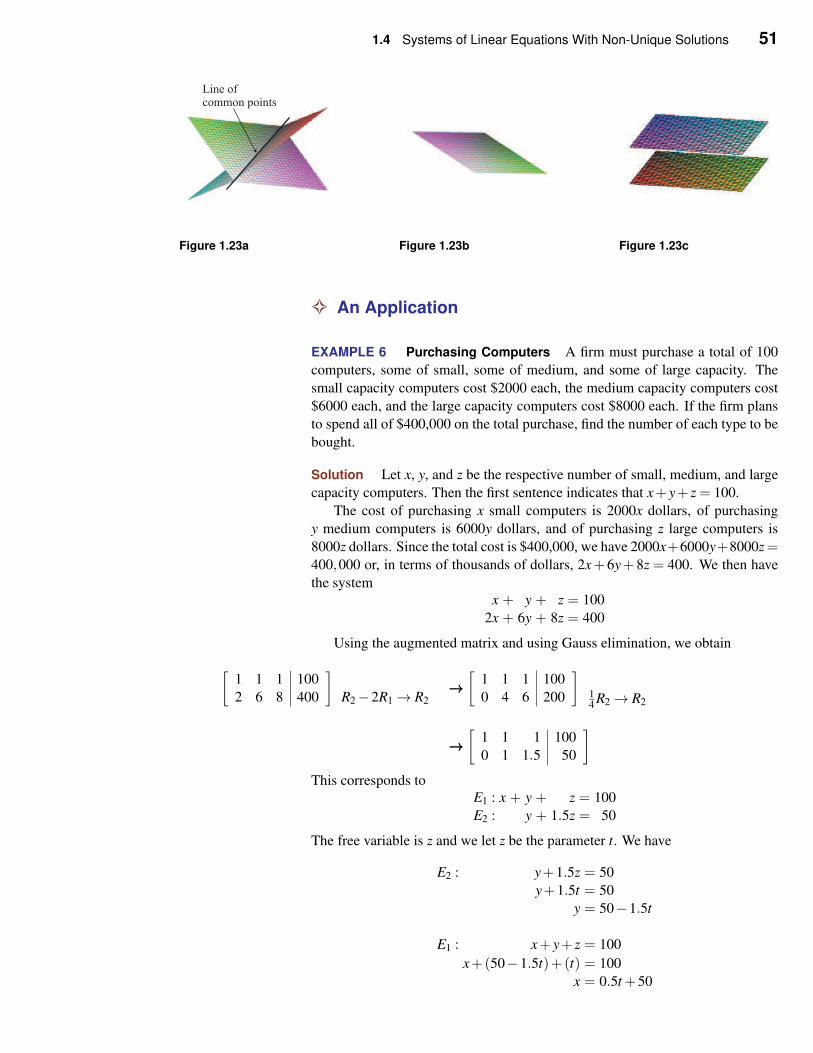
1.4 Systems of Linear Equations With Non-Unique Solutions 51
Line ofcommon points
Figure 1.23a Figure 1.23b Figure 1.23c
✧ An Application
EXAMPLE 6 Purchasing Computers A firm must purchase a total of 100
computers, some of small, some of medium, and some of large capacity. The
small capacity computers cost $2000 each, the medium capacity computers cost
$6000 each, and the large capacity computers cost $8000 each. If the firm plans
to spend all of $400,000 on the total purchase, find the number of each type to be
bought.
Solution Let x, y, and z be the respective number of small, medium, and large
capacity computers. Then the first sentence indicates that x+ y+ z = 100.
The cost of purchasing x small computers is 2000x dollars, of purchasing
y medium computers is 6000y dollars, and of purchasing z large computers is
8000z dollars. Since the total cost is $400,000, we have 2000x+6000y+8000z=400,000 or, in terms of thousands of dollars, 2x+ 6y+ 8z = 400. We then have
the systemx + y + z = 100
2x + 6y + 8z = 400
Using the augmented matrix and using Gauss elimination, we obtain
[1 1 1 100
2 6 8 400
]
R2−2R1→ R2→→→[
1 1 1 100
0 4 6 200
]
14 R2→ R2
→→→[
1 1 1 100
0 1 1.5 50
]
This corresponds toE1 : x + y + z = 100
E2 : y + 1.5z = 50
The free variable is z and we let z be the parameter t. We have
E2 : y+1.5z = 50
y+1.5t = 50
y = 50−1.5t
E1 : x+ y+ z = 100
x+(50−1.5t)+(t) = 100
x = 0.5t +50
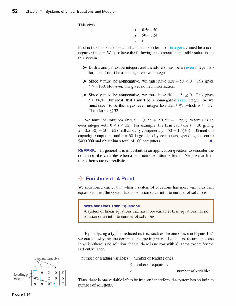
52 Chapter 1 Systems of Linear Equations and Models
This givesx = 0.5t +50
y = 50−1.5t
z = t
First notice that since t = z and z has units in terms of integers, t must be a non-
negative integer. We also have the following clues about the possible solutions to
this system
➤ Both x and y must be integers and therefore t must be an even integer. So
far, then, t must be a nonnegative even integer.
➤ Since x must be nonnegative, we must have 0.5t + 50 ≥ 0. This gives
t ≥−100. However, this gives no new information.
➤ Since y must be nonnegative, we must have 50− 1.5t ≥ 0. This gives
t ≤ 100/3. But recall that t must be a nonnegative even integer. So we
must take t to be the largest even integer less than 100/3, which is t = 32.
Therefore, t ≤ 32.
We have the solutions (x,y,z) = (0.5t + 50,50 − 1.5t, t), where t is an
even integer with 0 ≤ t ≤ 32. For example, the firm can take t = 30 giving
x= 0.5(30) + 50= 65 small capacity computers, y= 50 − 1.5(30)= 35 medium
capacity computers, and t = 30 large capacity computers, spending the entire
$400,000 and obtaining a total of 100 computers. ✦
REMARK: In general it is important in an application question to consider the
domain of the variables when a parametric solution is found. Negative or frac-
tional items are not realistic.
✧ Enrichment: A Proof
We mentioned earlier that when a system of equations has more variables than
equations, then the system has no solution or an infinite number of solutions.
More Variables Than Equations
A system of linear equations that has more variables than equations has no
solution or an infinite number of solutions.
By analyzing a typical reduced matrix, such as the one shown in Figure 1.24
we can see why this theorem must be true in general. Let us first assume the case
in which there is no solution; that is, there is no row with all zeros except for the
last entry. Then
number of leading variables = number of leading ones
≤ number of equations
< number of variables
Thus, there is one variable left to be free, and therefore, the system has an infinite
number of solutions.
x y z u
0 1 2 0 6
0 0 0 1 7
1 0 3 0 5
Leading variables
Leadingones
Figure 1.24
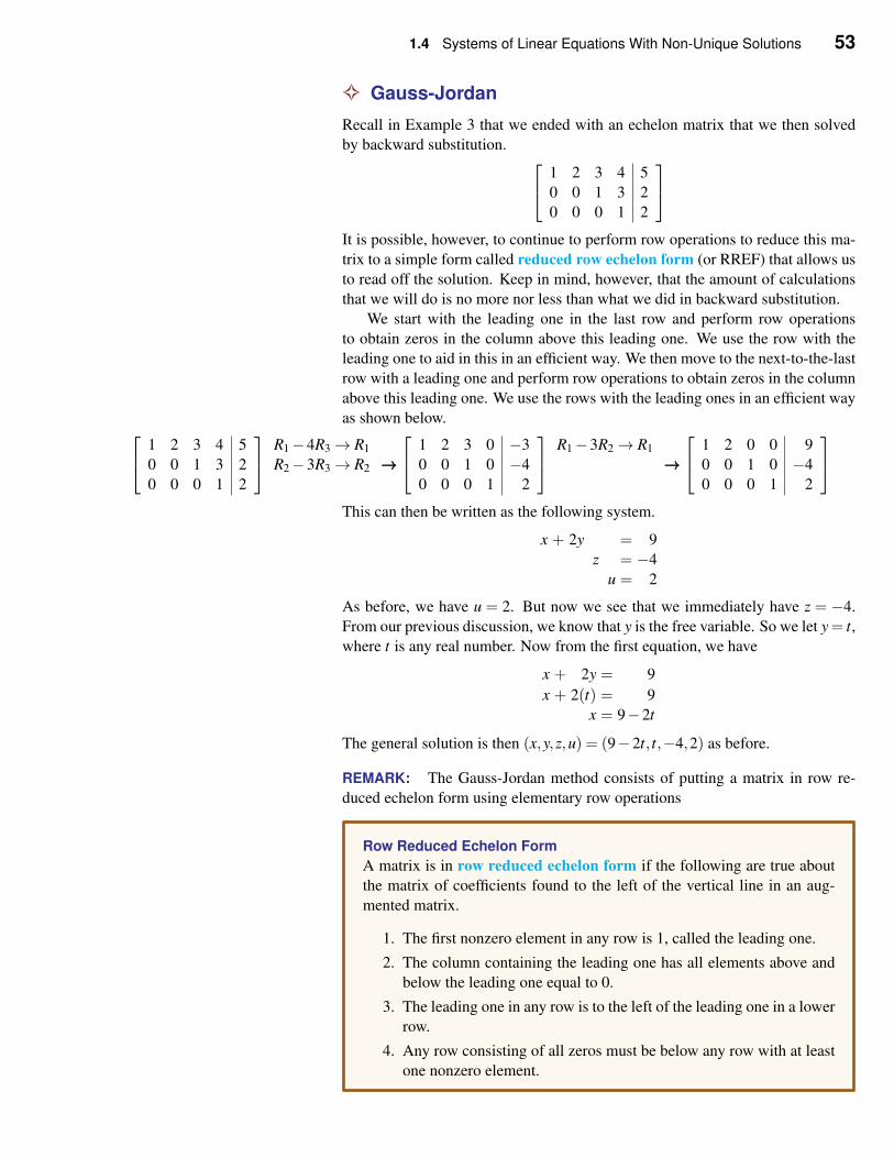
1.4 Systems of Linear Equations With Non-Unique Solutions 53
✧ Gauss-Jordan
Recall in Example 3 that we ended with an echelon matrix that we then solved
by backward substitution.
1 2 3 4 5
0 0 1 3 2
0 0 0 1 2
It is possible, however, to continue to perform row operations to reduce this ma-
trix to a simple form called reduced row echelon form (or RREF) that allows us
to read off the solution. Keep in mind, however, that the amount of calculations
that we will do is no more nor less than what we did in backward substitution.
We start with the leading one in the last row and perform row operations
to obtain zeros in the column above this leading one. We use the row with the
leading one to aid in this in an efficient way. We then move to the next-to-the-last
row with a leading one and perform row operations to obtain zeros in the column
above this leading one. We use the rows with the leading ones in an efficient way
as shown below.
1 2 3 4 5
0 0 1 3 2
0 0 0 1 2
R1−4R3→ R1
R2−3R3→ R2 →→→
1 2 3 0 −3
0 0 1 0 −4
0 0 0 1 2
R1−3R2→ R1
→→→
1 2 0 0 9
0 0 1 0 −4
0 0 0 1 2
This can then be written as the following system.
x + 2y = 9
z = −4
u = 2
As before, we have u = 2. But now we see that we immediately have z = −4.
From our previous discussion, we know that y is the free variable. So we let y= t,
where t is any real number. Now from the first equation, we have
x + 2y = 9
x + 2(t) = 9
x = 9−2t
The general solution is then (x,y,z,u) = (9−2t, t,−4,2) as before.
REMARK: The Gauss-Jordan method consists of putting a matrix in row re-
duced echelon form using elementary row operations
Row Reduced Echelon Form
A matrix is in row reduced echelon form if the following are true about
the matrix of coefficients found to the left of the vertical line in an aug-
mented matrix.
1. The first nonzero element in any row is 1, called the leading one.
2. The column containing the leading one has all elements above and
below the leading one equal to 0.
3. The leading one in any row is to the left of the leading one in a lower
row.
4. Any row consisting of all zeros must be below any row with at least
one nonzero element.
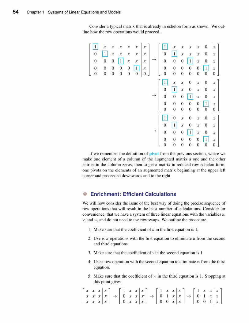
54 Chapter 1 Systems of Linear Equations and Models
Consider a typical matrix that is already in echelon form as shown. We out-
line how the row operations would proceed.
1 x x x x x x
0 1 x x x x x
0 0 0 1 x x x
0 0 0 0 0 1 x
0 0 0 0 0 0 0
→→→
1 x x x x 0 x
0 1 x x x 0 x
0 0 0 1 x 0 x
0 0 0 0 0 1 x
0 0 0 0 0 0 0
→→→
1 x x 0 x 0 x
0 1 x 0 x 0 x
0 0 0 1 x 0 x
0 0 0 0 0 1 x
0 0 0 0 0 0 0
→→→
1 0 x 0 x 0 x
0 1 x 0 x 0 x
0 0 0 1 x 0 x
0 0 0 0 0 1 x
0 0 0 0 0 0 0
If we remember the definition of pivot from the previous section, where we
make one element of a column of the augmented matrix a one and the other
entries in the column zeros, then to get a matrix in reduced row echelon form,
one pivots on the elements of an augmented matrix beginning at the upper left
corner and proceeded downwards and to the right.
✧ Enrichment: Efficient Calculations
We will now consider the issue of the best way of doing the precise sequence of
row operations that will result in the least number of calculations. Consider for
convenience, that we have a system of three linear equations with the variables u,
v, and w, and do not need to use row swaps. We outline the procedure.
1. Make sure that the coefficient of u in the first equation is 1.
2. Use row operations with the first equation to eliminate u from the second
and third equations.
3. Make sure that the coefficient of v in the second equation is 1.
4. Use a row operation with the second equation to eliminate w from the third
equation.
5. Make sure that the coefficient of w in the third equation is 1. Stopping at
this point gives
x x x x
x x x x
x x x x
→→→
1 x x x
0 x x x
0 x x x
→→→
1 x x x
0 1 x x
0 0 x x
→→→
1 x x x
0 1 x x
0 0 1 x
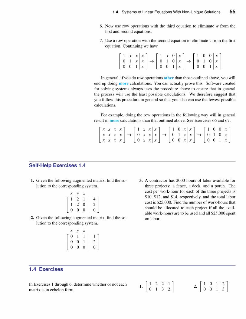
1.4 Systems of Linear Equations With Non-Unique Solutions 55
6. Now use row operations with the third equation to eliminate w from the
first and second equations.
7. Use a row operation with the second equation to eliminate v from the first
equation. Continuing we have
1 x x x
0 1 x x
0 0 1 x
→→→
1 x 0 x
0 1 0 x
0 0 1 x
→→→
1 0 0 x
0 1 0 x
0 0 1 x
In general, if you do row operations other than those outlined above, you will
end up doing more calculations. You can actually prove this. Software created
for solving systems always uses the procedure above to ensure that in general
the process will use the least possible calculations. We therefore suggest that
you follow this procedure in general so that you also can use the fewest possible
calculations.
For example, doing the row operations in the following way will in general
result in more calculations than that outlined above. See Exercises 66 and 67.
x x x x
x x x x
x x x x
→→→
1 x x x
0 x x x
0 x x x
→→→
1 0 x x
0 1 x x
0 0 x x
→→→
1 0 0 x
0 1 0 x
0 0 1 x
Self-Help Exercises 1.4
1. Given the following augmented matrix, find the so-
lution to the corresponding system.
x y z
1 2 1 4
1 2 0 2
0 0 0 0
2. Given the following augmented matrix, find the so-
lution to the corresponding system.
x y z
0 1 1 1
0 0 1 2
0 0 0 0
3. A contractor has 2000 hours of labor available for
three projects: a fence, a deck, and a porch. The
cost per work-hour for each of the three projects is
$10, $12, and $14, respectively, and the total labor
cost is $25,000. Find the number of work-hours that
should be allocated to each project if all the avail-
able work-hours are to be used and all $25,000 spent
on labor.
1.4 Exercises
In Exercises 1 through 6, determine whether or not each
matrix is in echelon form.1.
[1 2 2 1
0 1 3 2
]
2.
[1 0 1 2
0 0 1 3
]
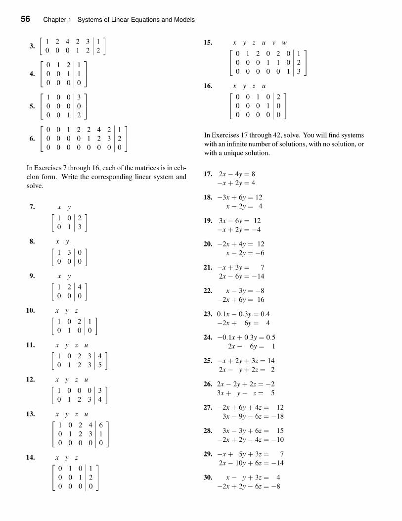
56 Chapter 1 Systems of Linear Equations and Models
3.
[1 2 4 2 3 1
0 0 0 1 2 2
]
4.
0 1 2 1
0 0 1 1
0 0 0 0
5.
1 0 0 3
0 0 0 0
0 0 1 2
6.
0 0 1 2 2 4 2 1
0 0 0 0 1 2 3 2
0 0 0 0 0 0 0 0
In Exercises 7 through 16, each of the matrices is in ech-
elon form. Write the corresponding linear system and
solve.
7. x y[
1 0 2
0 1 3
]
8. x y[
1 3 0
0 0 0
]
9. x y[
1 2 4
0 0 0
]
10. x y z[
1 0 2 1
0 1 0 0
]
11. x y z u[
1 0 2 3 4
0 1 2 3 5
]
12. x y z u[
1 0 0 0 3
0 1 2 3 4
]
13. x y z u
1 0 2 4 6
0 1 2 3 1
0 0 0 0 0
14. x y z
0 1 0 1
0 0 1 2
0 0 0 0
15. x y z u v w
0 1 2 0 2 0 1
0 0 0 1 1 0 2
0 0 0 0 0 1 3
16. x y z u
0 0 1 0 2
0 0 0 1 0
0 0 0 0 0
In Exercises 17 through 42, solve. You will find systems
with an infinite number of solutions, with no solution, or
with a unique solution.
17. 2x − 4y = 8
−x + 2y = 4
18. −3x + 6y = 12
x − 2y = 4
19. 3x − 6y = 12
−x + 2y = −4
20. −2x + 4y = 12
x − 2y = −6
21. −x + 3y = 7
2x − 6y = −14
22. x − 3y = −8
−2x + 6y = 16
23. 0.1x − 0.3y = 0.4−2x + 6y = 4
24. −0.1x + 0.3y = 0.52x − 6y = 1
25. −x + 2y + 3z = 14
2x − y + 2z = 2
26. 2x − 2y + 2z = −2
3x + y − z = 5
27. −2x + 6y + 4z = 12
3x − 9y − 6z = −18
28. 3x − 3y + 6z = 15
−2x + 2y − 4z = −10
29. −x + 5y + 3z = 7
2x − 10y + 6z = −14
30. x − y + 3z = 4
−2x + 2y − 6z = −8
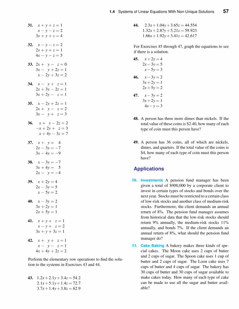
1.4 Systems of Linear Equations With Non-Unique Solutions 57
31. x + y + z = 1
x − y − z = 2
3x + y + z = 4
32. x − y − z = 2
2x + y + z = 1
4x − y − z = 5
33. 2x + y − z = 0
3x − y + 2z = 1
x − 2y + 3z = 2
34. x − y + z = 1
2x + 3y − 2z = 1
3x + 2y − z = 1
35. x − 2y + 2z = 1
2x + y − z = 2
3x − y + z = 3
36. x + y − 2z = 2
−x + 2y + z = 3
x + 4y − 3z = 7
37. x + y = 4
2x − 3y = −7
3x − 4y = −9
38. x − 3y = −7
3x + 4y = 5
2x − y = −4
39. x + 2y = 4
2x − 3y = 5
x − 5y = 2
40. x − 3y = 2
3x + 2y = 1
2x + 5y = 1
41. x + y + z = 1
x − y + z = 2
3x + y + 3z = 1
42. x + y + z = 1
x − y − z = 1
4x + 4y + 2z = 2
Perform the elementary row operations to find the solu-
tion to the systems in Exercises 43 and 44.
43. 1.2x+2.1y+3.4z = 54.22.1x+5.1y+1.4z = 72.73.7x+1.4y+3.8z = 62.9
44. 2.3x+1.04y+3.65z = 44.554
1.32x+2.87y+5.21z = 59.923
1.66x+1.92y+3.41z = 42.617
For Exercises 45 through 47, graph the equations to see
if there is a solution.
45. x+2y = 4
2x−3y = 5
x−5y = 3
46. x−3y = 2
3x+2y = 1
2x+5y = 2
47. x−3y = 2
3x+2y = 1
4x− y = 3
48. A person has three more dimes than nickels. If the
total value of these coins is $2.40, how many of each
type of coin must this person have?
49. A person has 36 coins, all of which are nickels,
dimes, and quarters. If the total value of the coins is
$4, how many of each type of coin must this person
have?
Applications
50. Investments A pension fund manager has been
given a total of $900,000 by a corporate client to
invest in certain types of stocks and bonds over the
next year. Stocks must be restricted to a certain class
of low-risk stocks and another class of medium-risk
stocks. Furthermore, the client demands an annual
return of 8%. The pension fund manager assumes
from historical data that the low-risk stocks should
return 9% annually, the medium-risk stocks 11%
annually, and bonds 7%. If the client demands an
annual return of 8%, what should the pension fund
manager do?
51. Cake Baking A bakery makes three kinds of spe-
cial cakes. The Moon cake uses 2 cups of butter
and 2 cups of sugar. The Spoon cake uses 1 cup of
butter and 2 cups of sugar. The Loon cake uses 7
cups of butter and 4 cups of sugar. The bakery has
30 cups of butter and 30 cups of sugar available to
make cakes today. How many of each type of cake
can be made to use all the sugar and butter avail-
able?
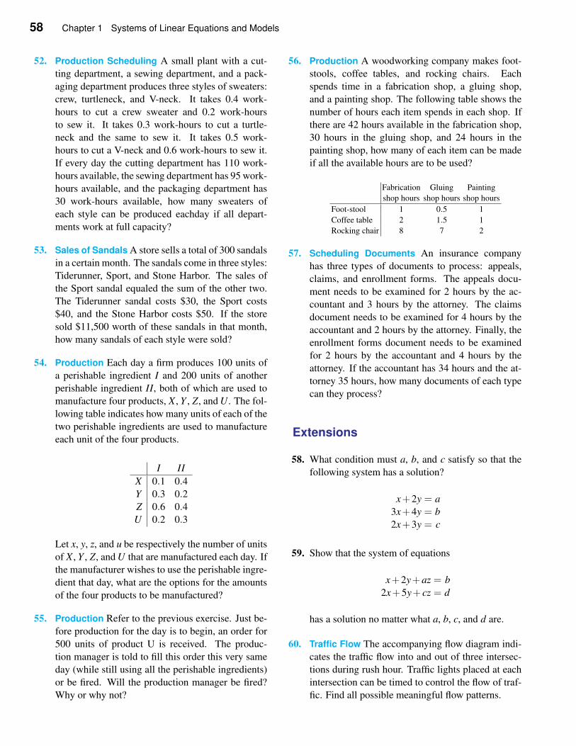
58 Chapter 1 Systems of Linear Equations and Models
52. Production Scheduling A small plant with a cut-
ting department, a sewing department, and a pack-
aging department produces three styles of sweaters:
crew, turtleneck, and V-neck. It takes 0.4 work-
hours to cut a crew sweater and 0.2 work-hours
to sew it. It takes 0.3 work-hours to cut a turtle-
neck and the same to sew it. It takes 0.5 work-
hours to cut a V-neck and 0.6 work-hours to sew it.
If every day the cutting department has 110 work-
hours available, the sewing department has 95 work-
hours available, and the packaging department has
30 work-hours available, how many sweaters of
each style can be produced eachday if all depart-
ments work at full capacity?
53. Sales of Sandals A store sells a total of 300 sandals
in a certain month. The sandals come in three styles:
Tiderunner, Sport, and Stone Harbor. The sales of
the Sport sandal equaled the sum of the other two.
The Tiderunner sandal costs $30, the Sport costs
$40, and the Stone Harbor costs $50. If the store
sold $11,500 worth of these sandals in that month,
how many sandals of each style were sold?
54. Production Each day a firm produces 100 units of
a perishable ingredient I and 200 units of another
perishable ingredient II, both of which are used to
manufacture four products, X , Y , Z, and U . The fol-
lowing table indicates how many units of each of the
two perishable ingredients are used to manufacture
each unit of the four products.
I II
X 0.1 0.4Y 0.3 0.2Z 0.6 0.4U 0.2 0.3
Let x, y, z, and u be respectively the number of units
of X , Y , Z, and U that are manufactured each day. If
the manufacturer wishes to use the perishable ingre-
dient that day, what are the options for the amounts
of the four products to be manufactured?
55. Production Refer to the previous exercise. Just be-
fore production for the day is to begin, an order for
500 units of product U is received. The produc-
tion manager is told to fill this order this very same
day (while still using all the perishable ingredients)
or be fired. Will the production manager be fired?
Why or why not?
56. Production A woodworking company makes foot-
stools, coffee tables, and rocking chairs. Each
spends time in a fabrication shop, a gluing shop,
and a painting shop. The following table shows the
number of hours each item spends in each shop. If
there are 42 hours available in the fabrication shop,
30 hours in the gluing shop, and 24 hours in the
painting shop, how many of each item can be made
if all the available hours are to be used?
Fabrication Gluing Painting
shop hours shop hours shop hours
Foot-stool 1 0.5 1
Coffee table 2 1.5 1
Rocking chair 8 7 2
57. Scheduling Documents An insurance company
has three types of documents to process: appeals,
claims, and enrollment forms. The appeals docu-
ment needs to be examined for 2 hours by the ac-
countant and 3 hours by the attorney. The claims
document needs to be examined for 4 hours by the
accountant and 2 hours by the attorney. Finally, the
enrollment forms document needs to be examined
for 2 hours by the accountant and 4 hours by the
attorney. If the accountant has 34 hours and the at-
torney 35 hours, how many documents of each type
can they process?
Extensions
58. What condition must a, b, and c satisfy so that the
following system has a solution?
x+2y = a
3x+4y = b
2x+3y = c
59. Show that the system of equations
x+2y+az = b
2x+5y+ cz = d
has a solution no matter what a, b, c, and d are.
60. Traffic Flow The accompanying flow diagram indi-
cates the traffic flow into and out of three intersec-
tions during rush hour. Traffic lights placed at each
intersection can be timed to control the flow of traf-
fic. Find all possible meaningful flow patterns.
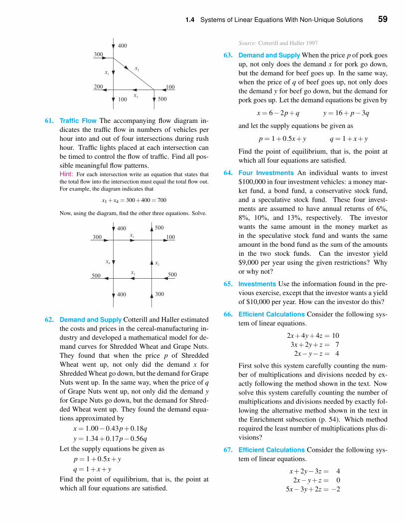
1.4 Systems of Linear Equations With Non-Unique Solutions 59
61. Traffic Flow The accompanying flow diagram in-
dicates the traffic flow in numbers of vehicles per
hour into and out of four intersections during rush
hour. Traffic lights placed at each intersection can
be timed to control the flow of traffic. Find all pos-
sible meaningful flow patterns.Hint: For each intersection write an equation that states that
the total flow into the intersection must equal the total flow out.
For example, the diagram indicates that
x1 + x4 = 300+400 = 700
Now, using the diagram, find the other three equations. Solve.
62. Demand and Supply Cotterill and Haller estimated
the costs and prices in the cereal-manufacturing in-
dustry and developed a mathematical model for de-
mand curves for Shredded Wheat and Grape Nuts.
They found that when the price p of Shredded
Wheat went up, not only did the demand x for
Shredded Wheat go down, but the demand for Grape
Nuts went up. In the same way, when the price of q
of Grape Nuts went up, not only did the demand y
for Grape Nuts go down, but the demand for Shred-
ded Wheat went up. They found the demand equa-
tions approximated by
x = 1.00−0.43p+0.18q
y = 1.34+0.17p−0.56q
Let the supply equations be given as
p = 1+0.5x+ y
q = 1+ x+ y
Find the point of equilibrium, that is, the point at
which all four equations are satisfied.
Source: Cotterill and Haller 1997
63. Demand and Supply When the price p of pork goes
up, not only does the demand x for pork go down,
but the demand for beef goes up. In the same way,
when the price of q of beef goes up, not only does
the demand y for beef go down, but the demand for
pork goes up. Let the demand equations be given by
x = 6−2p+q y = 16+ p−3q
and let the supply equations be given as
p = 1+0.5x+ y q = 1+ x+ y
Find the point of equilibrium, that is, the point at
which all four equations are satisfied.
64. Four Investments An individual wants to invest
$100,000 in four investment vehicles: a money mar-
ket fund, a bond fund, a conservative stock fund,
and a speculative stock fund. These four invest-
ments are assumed to have annual returns of 6%,
8%, 10%, and 13%, respectively. The investor
wants the same amount in the money market as
in the speculative stock fund and wants the same
amount in the bond fund as the sum of the amounts
in the two stock funds. Can the investor yield
$9,000 per year using the given restrictions? Why
or why not?
65. Investments Use the information found in the pre-
vious exercise, except that the investor wants a yield
of $10,000 per year. How can the investor do this?
66. Efficient Calculations Consider the following sys-
tem of linear equations.
2x+4y+4z = 10
3x+2y+ z = 7
2x− y− z = 4
First solve this system carefully counting the num-
ber of multiplications and divisions needed by ex-
actly following the method shown in the text. Now
solve this system carefully counting the number of
multiplications and divisions needed by exactly fol-
lowing the alternative method shown in the text in
the Enrichment subsection (p. 54). Which method
required the least number of multiplications plus di-
visions?
67. Efficient Calculations Consider the following sys-
tem of linear equations.
x+2y−3z = 4
2x− y+ z = 0
5x−3y+2z = −2
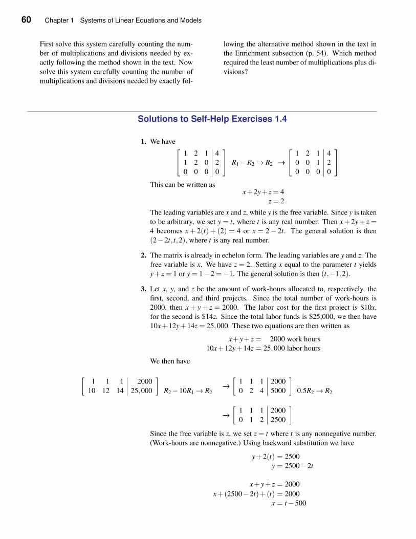
60 Chapter 1 Systems of Linear Equations and Models
First solve this system carefully counting the num-
ber of multiplications and divisions needed by ex-
actly following the method shown in the text. Now
solve this system carefully counting the number of
multiplications and divisions needed by exactly fol-
lowing the alternative method shown in the text in
the Enrichment subsection (p. 54). Which method
required the least number of multiplications plus di-
visions?
Solutions to Self-Help Exercises 1.4
1. We have
1 2 1 4
1 2 0 2
0 0 0 0
R1−R2→ R2 →→→
1 2 1 4
0 0 1 2
0 0 0 0
This can be written asx+2y+ z = 4
z = 2
The leading variables are x and z, while y is the free variable. Since y is taken
to be arbitrary, we set y = t, where t is any real number. Then x+ 2y+ z =4 becomes x+ 2(t) + (2) = 4 or x = 2− 2t. The general solution is then
(2−2t, t,2), where t is any real number.
2. The matrix is already in echelon form. The leading variables are y and z. The
free variable is x. We have z = 2. Setting x equal to the parameter t yields
y+ z = 1 or y = 1−2 =−1. The general solution is then (t,−1,2).
3. Let x, y, and z be the amount of work-hours allocated to, respectively, the
first, second, and third projects. Since the total number of work-hours is
2000, then x + y+ z = 2000. The labor cost for the first project is $10x,
for the second is $14z. Since the total labor funds is $25,000, we then have
10x+12y+14z = 25,000. These two equations are then written as
x+ y+ z = 2000 work hours
10x+12y+14z = 25,000 labor hours
We then have
[1 1 1 2000
10 12 14 25,000
]
R2−10R1→ R2→→→[
1 1 1 2000
0 2 4 5000
]
0.5R2→ R2
→→→[
1 1 1 2000
0 1 2 2500
]
Since the free variable is z, we set z = t where t is any nonnegative number.
(Work-hours are nonnegative.) Using backward substitution we have
y+2(t) = 2500
y = 2500−2t
x+ y+ z = 2000
x+(2500−2t)+(t) = 2000
x = t−500
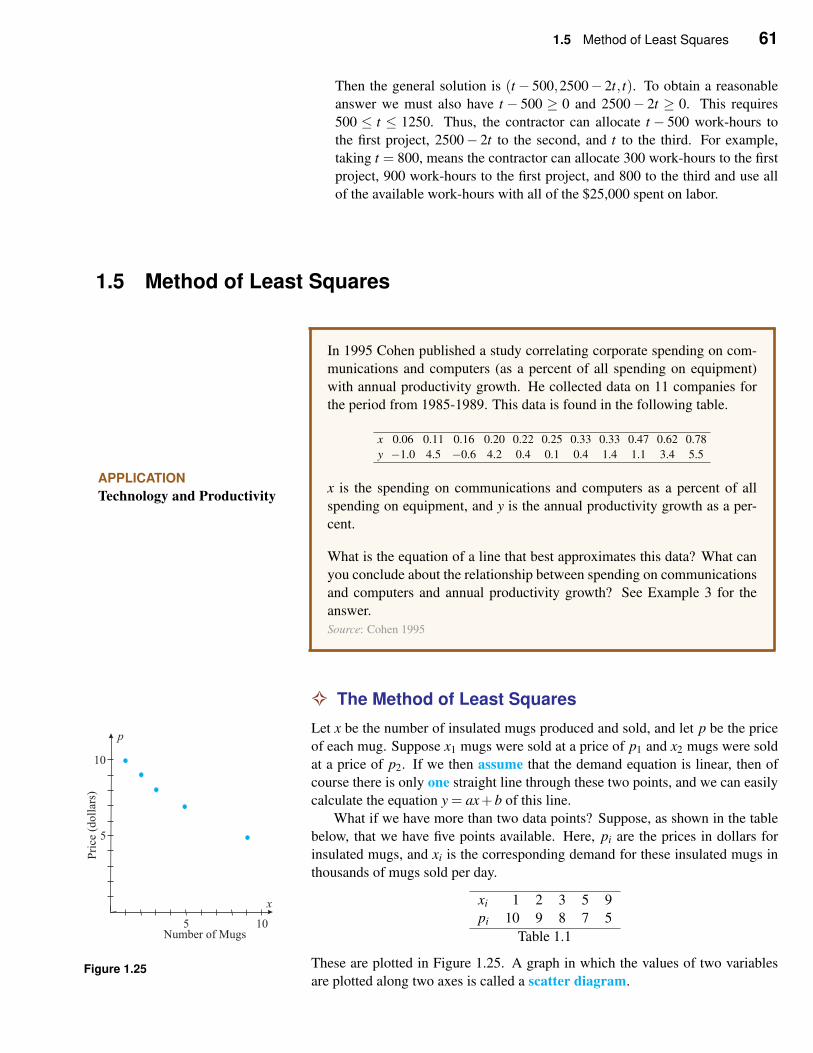
1.5 Method of Least Squares 61
Then the general solution is (t − 500,2500− 2t, t). To obtain a reasonable
answer we must also have t − 500 ≥ 0 and 2500− 2t ≥ 0. This requires
500 ≤ t ≤ 1250. Thus, the contractor can allocate t − 500 work-hours to
the first project, 2500− 2t to the second, and t to the third. For example,
taking t = 800, means the contractor can allocate 300 work-hours to the first
project, 900 work-hours to the first project, and 800 to the third and use all
of the available work-hours with all of the $25,000 spent on labor.
1.5 Method of Least Squares
APPLICATION
Technology and Productivity
In 1995 Cohen published a study correlating corporate spending on com-
munications and computers (as a percent of all spending on equipment)
with annual productivity growth. He collected data on 11 companies for
the period from 1985-1989. This data is found in the following table.
x 0.06 0.11 0.16 0.20 0.22 0.25 0.33 0.33 0.47 0.62 0.78
y −1.0 4.5 −0.6 4.2 0.4 0.1 0.4 1.4 1.1 3.4 5.5
x is the spending on communications and computers as a percent of all
spending on equipment, and y is the annual productivity growth as a per-
cent.
What is the equation of a line that best approximates this data? What can
you conclude about the relationship between spending on communications
and computers and annual productivity growth? See Example 3 for the
answer.
Source: Cohen 1995
✧ The Method of Least Squares
Let x be the number of insulated mugs produced and sold, and let p be the price
of each mug. Suppose x1 mugs were sold at a price of p1 and x2 mugs were sold
at a price of p2. If we then assume that the demand equation is linear, then of
course there is only one straight line through these two points, and we can easily
calculate the equation y = ax+b of this line.
What if we have more than two data points? Suppose, as shown in the table
below, that we have five points available. Here, pi are the prices in dollars for
insulated mugs, and xi is the corresponding demand for these insulated mugs in
thousands of mugs sold per day.
Figure 1.25
xi 1 2 3 5 9
pi 10 9 8 7 5
Table 1.1
These are plotted in Figure 1.25. A graph in which the values of two variables
are plotted along two axes is called a scatter diagram.
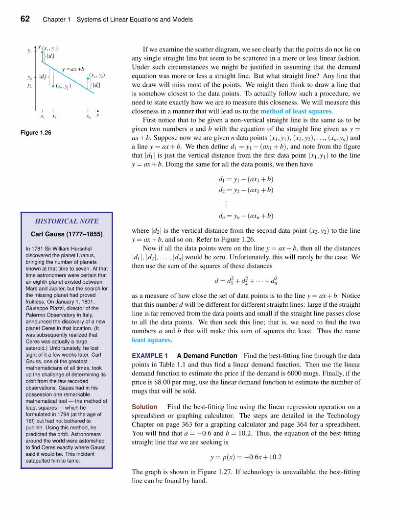
62 Chapter 1 Systems of Linear Equations and Models
If we examine the scatter diagram, we see clearly that the points do not lie on
any single straight line but seem to be scattered in a more or less linear fashion.
Under such circumstances we might be justified in assuming that the demand
equation was more or less a straight line. But what straight line? Any line that
we draw will miss most of the points. We might then think to draw a line that
is somehow closest to the data points. To actually follow such a procedure, we
need to state exactly how we are to measure this closeness. We will measure this
closeness in a manner that will lead us to the method of least squares.x
y
y = ax +b
|d1|
(x2, y
2)
x2 xnx1
( , )x y1 1
|d2|( , )x yn n
|dn |
y1
y2
yn
Figure 1.26
First notice that to be given a non-vertical straight line is the same as to be
given two numbers a and b with the equation of the straight line given as y =ax+b. Suppose now we are given n data points (x1,y1), (x2,y2), . . ., (xn,yn) and
a line y = ax+ b. We then define d1 = y1− (ax1 + b), and note from the figure
that |d1| is just the vertical distance from the first data point (x1,y1) to the line
y = ax+b. Doing the same for all the data points, we then have
d1 = y1− (ax1 +b)
d2 = y2− (ax2 +b)
...
dn = yn− (axn +b)
where |d2| is the vertical distance from the second data point (x2,y2) to the line
y = ax+b, and so on. Refer to Figure 1.26.
Now if all the data points were on the line y = ax+ b, then all the distances
|d1|, |d2|, . . . , |dn| would be zero. Unfortunately, this will rarely be the case. We
then use the sum of the squares of these distances
d = d21 +d2
2 + · · ·+d2n
as a measure of how close the set of data points is to the line y = ax+b. Notice
that this number d will be different for different straight lines: large if the straight
line is far removed from the data points and small if the straight line passes close
to all the data points. We then seek this line; that is, we need to find the two
numbers a and b that will make this sum of squares the least. Thus the name
least squares.
HISTORICAL NOTE
Carl Gauss (1777–1855)
In 1781 Sir William Herschel
discovered the planet Uranus,
bringing the number of planets
known at that time to seven. At that
time astronomers were certain that
an eighth planet existed between
Mars and Jupiter, but the search for
the missing planet had proved
fruitless. On January 1, 1801,
Giuseppe Piazzi, director of the
Palermo Observatory in Italy,
announced the discovery of a new
planet Ceres in that location. (It
was subsequently realized that
Ceres was actually a large
asteroid.) Unfortunately, he lost
sight of it a few weeks later. Carl
Gauss, one of the greatest
mathematicians of all times, took
up the challenge of determining its
orbit from the few recorded
observations. Gauss had in his
possession one remarkable
mathematical tool — the method of
least squares — which he
formulated in 1794 (at the age of
16!) but had not bothered to
publish. Using this method, he
predicted the orbit. Astronomers
around the world were astonished
to find Ceres exactly where Gauss
said it would be. This incident
catapulted him to fame.
EXAMPLE 1 A Demand Function Find the best-fitting line through the data
points in Table 1.1 and thus find a linear demand function. Then use the linear
demand function to estimate the price if the demand is 6000 mugs. Finally, if the
price is $8.00 per mug, use the linear demand function to estimate the number of
mugs that will be sold.
Solution Find the best-fitting line using the linear regression operation on a
spreadsheet or graphing calculator. The steps are detailed in the Technology
Chapter on page 363 for a graphing calculator and page 364 for a spreadsheet.
You will find that a = −0.6 and b = 10.2. Thus, the equation of the best-fitting
straight line that we are seeking is
y = p(x) =−0.6x+10.2
The graph is shown in Figure 1.27. If technology is unavailable, the best-fitting
line can be found by hand.
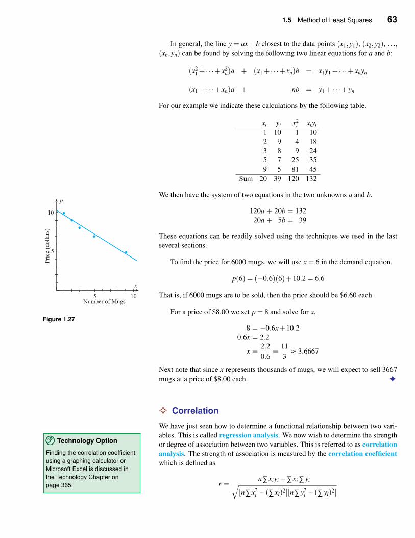
1.5 Method of Least Squares 63
In general, the line y = ax+b closest to the data points (x1,y1), (x2,y2), . . .,(xn,yn) can be found by solving the following two linear equations for a and b:
(x21 + · · ·+ x2
n)a + (x1 + · · ·+ xn)b = x1y1 + · · ·+ xnyn
(x1 + · · ·+ xn)a + nb = y1 + · · ·+ yn
For our example we indicate these calculations by the following table.
xi yi x2i xiyi
1 10 1 10
2 9 4 18
3 8 9 24
5 7 25 35
9 5 81 45
Sum 20 39 120 132
We then have the system of two equations in the two unknowns a and b.
Figure 1.27
120a + 20b = 132
20a + 5b = 39
These equations can be readily solved using the techniques we used in the last
several sections.
To find the price for 6000 mugs, we will use x = 6 in the demand equation.
p(6) = (−0.6)(6)+10.2 = 6.6
That is, if 6000 mugs are to be sold, then the price should be $6.60 each.
For a price of $8.00 we set p = 8 and solve for x,
8 = −0.6x+10.20.6x = 2.2
x =2.2
0.6=
11
3≈ 3.6667
Next note that since x represents thousands of mugs, we will expect to sell 3667
mugs at a price of $8.00 each. ✦
✧ Correlation
We have just seen how to determine a functional relationship between two vari-
ables. This is called regression analysis. We now wish to determine the strength
or degree of association between two variables. This is referred to as correlation
analysis. The strength of association is measured by the correlation coefficient
which is defined as
TTT©©© Technology Option
Finding the correlation coefficient
using a graphing calculator or
Microsoft Excel is discussed in
the Technology Chapter on
page 365. r =n∑xiyi−∑xi ∑yi
√
[n∑x2i − (∑xi)2][n∑y2
i − (∑yi)2]
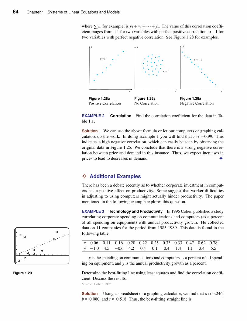
64 Chapter 1 Systems of Linear Equations and Models
where ∑yi, for example, is y1 +y2+ · · ·+yn. The value of this correlation coeffi-
cient ranges from +1 for two variables with perfect positive correlation to−1 for
two variables with perfect negative correlation. See Figure 1.28 for examples.
Figure 1.28a
Positive Correlation
Figure 1.28a
No Correlation
Figure 1.28a
Negative Correlation
EXAMPLE 2 Correlation Find the correlation coefficient for the data in Ta-
ble 1.1.
Solution We can use the above formula or let our computers or graphing cal-
culators do the work. In doing Example 1 you will find that r ≈ −0.99. This
indicates a high negative correlation, which can easily be seen by observing the
original data in Figure 1.25. We conclude that there is a strong negative corre-
lation between price and demand in this instance. Thus, we expect increases in
prices to lead to decreases in demand. ✦
✧ Additional Examples
There has been a debate recently as to whether corporate investment in comput-
ers has a positive effect on productivity. Some suggest that worker difficulties
in adjusting to using computers might actually hinder productivity. The paper
mentioned in the following example explores this question.
EXAMPLE 3 Technology and Productivity In 1995 Cohen published a study
correlating corporate spending on communications and computers (as a percent
of all spending on equipment) with annual productivity growth. He collected
data on 11 companies for the period from 1985-1989. This data is found in the
following table.
x 0.06 0.11 0.16 0.20 0.22 0.25 0.33 0.33 0.47 0.62 0.78
y −1.0 4.5 −0.6 4.2 0.4 0.1 0.4 1.4 1.1 3.4 5.5
x is the spending on communications and computers as a percent of all spend-
ing on equipment, and y is the annual productivity growth as a percent.
Figure 1.29 Determine the best-fitting line using least squares and find the correlation coeffi-
cient. Discuss the results.
Source: Cohen 1995
Solution Using a spreadsheet or a graphing calculator, we find that a≈ 5.246,
b≈ 0.080, and r ≈ 0.518. Thus, the best-fitting straight line is
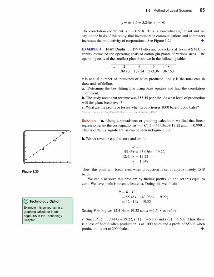
1.5 Method of Least Squares 65
y = ax+b = 5.246x+0.080
The correlation coefficient is r = 0.518. This is somewhat significant and we
say, on the basis of this study, that investment in communications and computers
increases the productivity of corporations. See Figure 1.29 ✦
EXAMPLE 4 Plant Costs In 1997 Fuller and coworkers at Texas A&M Uni-
versity estimated the operating costs of cotton gin plants of various sizes. The
operating costs of the smallest plant is shown in the following table.
x 2 4 6 8
y 109.40 187.24 273.36 367.60
x is annual number of thousands of bales produced, and y is the total cost in
thousands of dollars
a. Determine the best-fitting line using least squares and find the correlation
coefficient.
b. The study noted that revenue was $55.45 per bale. At what level of production
will this plant break even?
c. What are the profits or losses when production is 1000 bales? 2000 bales?
Source: Fuller, Gillis, Parnell, Ramaiyer, and Childers 1997
Solution a. Using a spreadsheet or graphing calculator, we find that linear
regression gives the cost equation as y=C(x) = 43.036x+19.22 and r = 0.9991.
Figure 1.30
This is certainly significant, as can be seen in Figure 1.30.
b. We set revenue equal to cost and obtain
R = C
55.45x = 43.036x+19.22
12.414x = 19.22
x = 1.548
Thus, this plant will break even when production is set at approximately 1548
bales.
We can also solve this problem by finding profits, P, and set this equal to
zero. We have profit is revenue less cost. Doing this we obtain
P = R−C
= 55.45x− (43.036x+19.22)= 12.414x−19.22
Setting P = 0, gives 12.414x = 19.22 and x = 1.548 as before.
TTT©©© Technology Option
Example 4 is solved using a
graphing calculator in on
page 365 in the Technology
Chapter c. Since P(x) = 12.414x−19.22, P(1) =−6.806 and P(2) = 5.608. Thus, there
is a loss of $6806 when production is at 1000 bales and a profit of $5608 when
production is set at 2000 bales. ✦
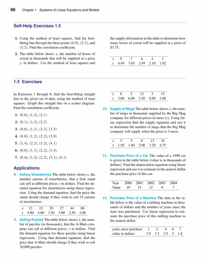
66 Chapter 1 Systems of Linear Equations and Models
Self-Help Exercises 1.5
1. Using the method of least squares, find the best-
fitting line through the three points (0,0), (2,2), and
(3,2). Find the correlation coefficient.
2. The table below shows x, the number of boxes of
cereal in thousands that will be supplied at a price
y, in dollars. Use the method of least squares and
the supply information in the table to determine how
many boxes of cereal will be supplied at a price of
$3.75.
x 9 7 6 4 3
y 4.49 3.05 2.49 2.10 1.92
1.5 Exercises
In Exercises 1 through 8, find the best-fitting straight
line to the given set of data, using the method of least
squares. Graph this straight line on a scatter diagram.
Find the correlation coefficient.
1. (0,0), (1,2), (2,1)
2. (0,1), (1,2), (2,2)
3. (0,0), (1,1), (2,3), (3,3)
4. (0,0), (1,2), (2,2), (3,0)
5. (1,4), (2,2), (3,2), (4,1)
6. (0,0), (1,1), (2,2), (3,4)
7. (0,4), (1,2), (2,2), (3,1), (4,1)
Applications
8. Selling Strawberries The table below shows x, the
number cartons of strawberries, that a fruit stand
can sell at different prices y in dollars. Find the de-
mand equation for strawberries using linear regres-
sion. Using the demand equation, find the price the
stand should charge if they wish to sell 35 cartons
of strawberries.
x 12 15 20 27 44 60
y 5.00 4.00 3.50 3.00 2.50 2.00
9. Selling Puzzles The table below shows x, the num-
ber of puzzles (in thousands), that the A-Mart com-
pany can sell at different prices, y in dollars. Find
the demand equation for these puzzles using linear
regression. Using that demand equation, find the
price that A-Mart should charge if they wish to sell
10,000 puzzles.
x 8 5 12 3 15
y 5.00 6.00 3.50 8.00 3.00
10. Supply of Mugs The table below shows x, the num-
ber of mugs in thousands supplied by the Big Mug
company for different prices in euros (y). Using lin-
ear regression find the supply equation and use it
to determine the number of mugs that the Big Mug
company will supply when the price is 3 euros.
x 3 5 6 13 18
y 1.50 1.80 2.00 3.20 4.75
11. Purchase Price of a Car The value of a 1998 car
is given in the table below (value is in thousands of
dollars). Find the depreciation equation using linear
regression and use it to estimate to the nearest dollar
the purchase price of this car.
Year 2000 2001 2002 2003 2004
Value 19 15 12 9 7
12. Purchase Price of a Machine The data in the ta-
ble below is the value of a milling machine in thou-
sands of dollars and the number of years since the
item was purchased. Use linear regression to esti-
mate the purchase price of this milling machine to
the nearest dollar.
years since purchase 1 2 4 6 7
value in dollars 3.9 3.2 2.5 2 1.8
1.5 Method of Least Squares 67
Referenced Applications
13. Deer Population and Deer-Vehicle Accidents
Rondeau and Conrad studied the relationship of
deer population in urban areas to accidents with ve-
hicles on roads. Below is the data where x is the deer
population in Irondequoit, NY, and y is the number
of collisions with deer in the same city.
x 340 350 480 510 515 600 650
y 150 60 90 130 120 110 140
x 700 760 765 820 850
y 120 210 170 180 230
a. Determine the best-fitting line using least
squares and the correlation coefficient.
b. Explain what the linear model is saying about
the deer population and collisions.
Source: Rondeau and Conrad 2003
14. Economies of Scale in Plant Size Strategic Man-
agement relates a study in economies of scale in the
machine-tool industry. The data is found in the fol-
lowing table,
x 70 115 130 190 195 400 450
y 1.1 1.0 0.85 0.75 0.85 0.67 0.50
where x is the plant capacity in thousands of units,
and y is the employee-hours per unit.
a. Determine the best-fitting line using least
squares and the correlation coefficient.
b. Is there an advantage in having a large plant?
Explain.
c. What does this model predict the employee-
hours per unit will be when the plant capacity
is 300,000 units?
d. What does this model predict the plant capacity
will be if the employee-hours per unit is 0.90?
Source: Rowe, Mason, Dickel, Mann, and Mockler 1994
15. Cost Curve Dean made a statistical estimation of
the cost-output relationship in a hosiery mill. The
data is given in the following table,
x 16 31 48 57 63 103 110
y 30 60 100 130 135 230 230
x 114 116 117 118 123 126
y 235 245 250 235 250 260
where x is the output in thousands of dozens and y
is the total cost in thousands of dollars.
a. Determine the best-fitting line using least
squares and find the correlation coefficient.
Graph.
b. What does this model predict the total cost will
be when the output is 100,000 dozen?
c. What does this model predict the output will be
if the total cost is $125,000?Source: Dean 1976
16. Cost Curve Johnston estimated the cost-output re-
lationship for 40 firms. The data for the fifth firm is
given in the following table where x is the output in
millions of units and y is the total cost in thousands
of pounds sterling
x 180 210 215 230 260 290 340 400
y 130 180 205 190 215 220 250 300
x 405 430 430 450 470 490 510
y 285 305 325 330 330 340 375
a. Determine the best-fitting line using least
squares and find the correlation coefficient.
Graph.
b. What does this model predict the total cost will
be when the output is 300 million units?
c. What does this model predict the output will be
if the total cost is 200,000 of pounds sterling?Source: Johnston 1960
17. Productivity Bernstein studied the correlation be-
tween productivity growth and gross national prod-
uct (GNP) growth of six countries. The countries
were France (F), Germany (G), Italy (I), Japan (J),
the United Kingdom (UK), and the United States
(US). Productivity is given as output per employee-
hour in manufacturing. The data they collected for
the years 1950–1977 is given in the following table
where x is the productivity growth (%) and y is the
GNP growth (%).
US UK F I G J
x 2.5 2.7 5.2 5.6 5.7 9.0
y 3.5 2.3 4.9 4.9 5.7 8.5
a. Determine the best-fitting line using least
squares and the correlation coefficient.
b. What does this model predict the GNP growth
will be when the productivity growth is 7 per-
cent?
c. What does this model predict the productivity
growth will be if the GNP growth is 7%?Source: Berstein 1980
68 Chapter 1 Systems of Linear Equations and Models
18. Productivity Recall from Example 3 that Cohen
studied the correlation between corporate spending
on communications and computers (as a percent of
all spending on equipment) and annual productivity
growth. In Example 3 we looked at his data on 11
companies for the period from 1985 to 1989. The
data found in the following table is for the years
1977–1984 where x is the spending on communica-
tions and computers as a percent of all spending on
equipment and y is the annual productivity growth.
x 0.03 0.07 0.10 0.13 0.14 0.17
y −2.0 −1.5 1.7 −0.6 2.2 0.3
x 0.24 0.29 0.39 0.62 0.83
y 1.3 4.2 3.4 4.0 −0.5
Determine the best-fitting line using least squares
and the correlation coefficient.
Source: Cohen 1995
19. Environmental Entomology The fall armyworm
has historically been a severe agricultural pest. How
the age at first mating of the female of this pest af-
fected its fecundity as measured by the number of
viable larvae resulting from the eggs laid has been
studied. The data is shown in following table, where
x is the age of first mating of the female in days and
y is the total number of viable larvae per female.
x 1 1 3 4 4 6
y 1650 1450 550 1150 650 850
x 6 8 10 10 12 13 15
y 800 450 900 500 100 100 200
Determine the best-fitting line using least squares.
Also determine the correlation coefficient.
Source: Rogers and O. G. Marti 1994
20. Plant Resistance Talekar and Lin collected the data
shown in the table that relates the pod diameter
(seed size) of soybeans to the percentage of pods
damaged by the limabean pod borer.
x 3.1 3.4 3.9 4.1 4.2 4.5
y 12 28 38 37 44 48
x is the pod diameter in mm and y is the percentage
of damaged pods.
a. Use linear regression to find the best-fitting line
that relates the pod diameter to the percentage of
pods damaged.
b. Find the correlation coefficient.
c. Interpret what the slope of the line means.
Source: Talekar and Lin 1994
21. Horticultural Entomology The brown citrus aphid
and the melon aphid both spread the citrus tris-
teza virus to fruit, and thus, have become impor-
tant pests. Yokomi and coworkers collected the data
found in the following table.
x 1 5 10 20
y 25 22 50 85
z 10 5 18 45
x is the number of aphids per plant, y and z are the
percentage of times the virus is transmitted to the
fruit for the brown and melon aphid, respectively.
a. Use linear regression for each aphid to find the
best-fitting line that relates the number of aphids
per plant to the percentage of times the virus is
transmitted to the fruit.
b. Find the correlation coefficients.
c. Interpret what the slope of the line means in each
case.
d. Which aphid is more destructive? Why?
Source: Yokomi, Lastra, Stoetzel, Damsteegt, Lee, Garnsey,
Gottwald, Rocha-Pena, and Niblett 1994
22. Biological Control Briano and colleagues studied
the host-pathogen relationship between the black
imported fire ant and a microsporidium (T. solenop-
sae) that infects them. The fire ant represents a seri-
ous medical and agricultural pest. The study was to
determine whether T. solenopae could be used as a
biological control of the imported fire ants. The ta-
ble includes data that they collected and relates the
number of colonies per hectare of the ants with the
percentage that are infected with T. Solenopsae.
x 23 30 32 50 72 74 79 81 98 110
y 27 35 50 34 14 25 15 33 23 26
x 116 122 132 138 140 150 150 152 162
y 18 28 19 23 22 18 24 21 22
x is the colonies of ants per hectare, and y is the per-
centage of infected colonies.
a. Use linear regression to find the best-fitting line
that relates the number of colonies of ants per
hectare to the percentage of infected colonies.
b. Find the correlation coefficient.
c. Interpret what the slope of the line means.
Source: Briano, Patterson, and Cordo 1995
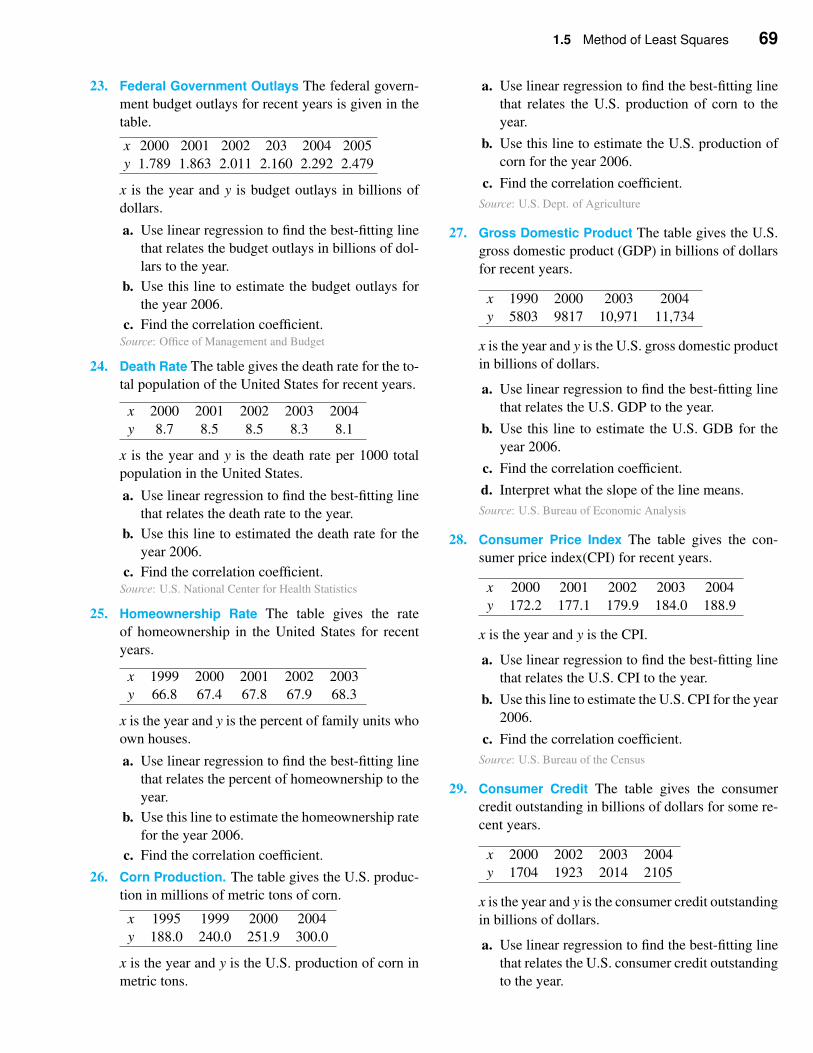
1.5 Method of Least Squares 69
23. Federal Government Outlays The federal govern-
ment budget outlays for recent years is given in the
table.
x 2000 2001 2002 203 2004 2005
y 1.789 1.863 2.011 2.160 2.292 2.479
x is the year and y is budget outlays in billions of
dollars.
a. Use linear regression to find the best-fitting line
that relates the budget outlays in billions of dol-
lars to the year.
b. Use this line to estimate the budget outlays for
the year 2006.
c. Find the correlation coefficient.Source: Office of Management and Budget
24. Death Rate The table gives the death rate for the to-
tal population of the United States for recent years.
x 2000 2001 2002 2003 2004
y 8.7 8.5 8.5 8.3 8.1
x is the year and y is the death rate per 1000 total
population in the United States.
a. Use linear regression to find the best-fitting line
that relates the death rate to the year.
b. Use this line to estimated the death rate for the
year 2006.
c. Find the correlation coefficient.Source: U.S. National Center for Health Statistics
25. Homeownership Rate The table gives the rate
of homeownership in the United States for recent
years.
x 1999 2000 2001 2002 2003
y 66.8 67.4 67.8 67.9 68.3
x is the year and y is the percent of family units who
own houses.
a. Use linear regression to find the best-fitting line
that relates the percent of homeownership to the
year.
b. Use this line to estimate the homeownership rate
for the year 2006.
c. Find the correlation coefficient.
26. Corn Production. The table gives the U.S. produc-
tion in millions of metric tons of corn.
x 1995 1999 2000 2004
y 188.0 240.0 251.9 300.0
x is the year and y is the U.S. production of corn in
metric tons.
a. Use linear regression to find the best-fitting line
that relates the U.S. production of corn to the
year.
b. Use this line to estimate the U.S. production of
corn for the year 2006.
c. Find the correlation coefficient.
Source: U.S. Dept. of Agriculture
27. Gross Domestic Product The table gives the U.S.
gross domestic product (GDP) in billions of dollars
for recent years.
x 1990 2000 2003 2004
y 5803 9817 10,971 11,734
x is the year and y is the U.S. gross domestic product
in billions of dollars.
a. Use linear regression to find the best-fitting line
that relates the U.S. GDP to the year.
b. Use this line to estimate the U.S. GDB for the
year 2006.
c. Find the correlation coefficient.
d. Interpret what the slope of the line means.
Source: U.S. Bureau of Economic Analysis
28. Consumer Price Index The table gives the con-
sumer price index(CPI) for recent years.
x 2000 2001 2002 2003 2004
y 172.2 177.1 179.9 184.0 188.9
x is the year and y is the CPI.
a. Use linear regression to find the best-fitting line
that relates the U.S. CPI to the year.
b. Use this line to estimate the U.S. CPI for the year
2006.
c. Find the correlation coefficient.
Source: U.S. Bureau of the Census
29. Consumer Credit The table gives the consumer
credit outstanding in billions of dollars for some re-
cent years.
x 2000 2002 2003 2004
y 1704 1923 2014 2105
x is the year and y is the consumer credit outstanding
in billions of dollars.
a. Use linear regression to find the best-fitting line
that relates the U.S. consumer credit outstanding
to the year.
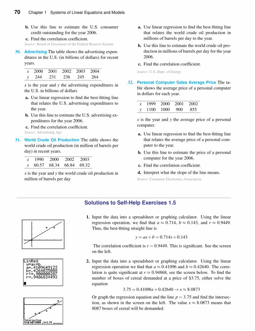
70 Chapter 1 Systems of Linear Equations and Models
b. Use this line to estimate the U.S. consumer
credit outstanding for the year 2006.
c. Find the correlation coefficient.Source: Board of Governors of the Federal Reserve System
30. Advertising The table shows the advertising expen-
ditures in the U.S. (in billions of dollars) for recent
years.
x 2000 2001 2002 2003 2004
y 244 231 236 245 264
x is the year and y the advertising expenditures in
the U.S. in billions of dollars
a. Use linear regression to find the best-fitting line
that relates the U.S. advertising expenditures to
the year.
b. Use this line to estimate the U.S. advertising ex-
penditures for the year 2006.
c. Find the correlation coefficient.Source: Advertising Age
31. World Crude Oil Production The table shows the
world crude oil production (in million of barrels per
day) in recent years.
x 1990 2000 2002 2003
y 60.57 68.34 66.84 69.32
x is the year and y the world crude oil production in
million of barrels per day
a. Use linear regression to find the best-fitting line
that relates the world crude oil production in
millions of barrels per day to the year.
b. Use this line to estimate the world crude oil pro-
duction in millions of barrels per day for the year
2006.
c. Find the correlation coefficient.
Source: U.S. Dept. of Energy
32. Personal Computer Sales Average Price The ta-
ble shows the average price of a personal computer
in dollars for each year.
x 1999 2000 2001 2002
y 1100 1000 900 855
x is the year and y the average price of a personal
computer.
a. Use linear regression to find the best-fitting line
that relates the average price of a personal com-
puter to the year.
b. Use this line to estimate the price of a personal
computer for the year 2006.
c. Find the correlation coefficient.
d. Interpret what the slope of the line means.
Source: Consumer Electronics Association
Solutions to Self-Help Exercises 1.5
1. Input the data into a spreadsheet or graphing calculator. Using the linear
regression operation, we find that a ≈ 0.714, b ≈ 0.143, and r ≈ 0.9449.
Thus, the best-fitting straight line is
y = ax+b = 0.714x+0.143
The correlation coefficient is r = 0.9449. This is significant. See the screen
on the left.
2. Input the data into a spreadsheet or graphing calculator. Using the linear
regression operation we find that a ≈ 0.41096 and b ≈ 0.42640. The corre-
lation is quite significant at r ≈ 0.94868, see the screen below. To find the
number of boxes of cereal demanded at a price of $3.75, either solve the
equation
3.75 = 0.41096x+0.42640→ x≈ 8.0873
Or graph the regression equation and the line p = 3.75 and find the intersec-
tion, as shown in the screen on the left. The value x ≈ 8.0873 means that
8087 boxes of cereal will be demanded.
Chapter 1 Review 71
Review
✧ Summary Outline
• A function f from the set D to the set R is a rule that assigns to each
element x in D one and only one element y = f (x) in R.
• The set D above is called the domain.
• One thinks of the domain as the set of inputs and the values y = f (x) as the
outputs.
• The set of all possible outputs is called the range.
• The letter representing the elements in the domain is called the indepen-
dent variable.
• The letter representing the elements in the range is called the dependent
variable.
• The graph of the function f consists of all points (x,y) such that x is in the
domain of f and y = f (x).
• Linear Cost, Revenue, and Profit Equations. Let x be the number of
items made and sold.
variable cost = (cost per item) × (number of items produced) = mx.
C = cost = (variable cost) + (fixed cost) = mx+b.
R = revenue = (price per item) × (number sold) = px.
P = profit = (revenue) − (cost) = R−C.
• The quantity at which the profit is zero is called the break-even quantity.
• Let x be the number of items made and sold and p the price of each item.
A linear demand equation, which governs the behavior of the consumer,
is of the form p = mx+ b, where m must be negative. A linear supply
equation, which governs the behavior of the producer, is of the form p =mx+b, where m must be positive.
• The point at which supply equals demand is called the equilibrium point.
The x-coordinate of the equilibrium point is called the equilibrium quan-
tity, and the p-coordinate is called the equilibrium price.
• A system of linear equations is a set of linear equations.
• The set of all solutions to a system of linear equations is called the solution
set.
• Two systems of equations with the same solution set are said to be equiv-
alent.
• A matrix is a rectangular array of numbers.
72 Chapter 1 Systems of Linear Equations and Models
• There are three elementary operations performed on a system of equa-
tions (matrix). Interchange two equations (rows). Replace an equation
(row) with a constant times the equation (row). Replace an equation (row)
plus a constant times another equation (row).
• Elementary operations yield an equivalent system of equations.
• Gauss elimination is a procedure for a systematically using elementary
operations to reduce a system of linear equations to an equivalent system
whose solution set can be immediately determined by backward substitu-
tion.
• There are three possibilities in solving a system of linear equations: There
can be precisely one solution. There can be no solution. There can be
infinitely many solutions.
• A matrix is in echelon form if:
1. The first nonzero element in any row is 1, called the leading one.
2. The column containing the leading one has all elements below the
leading one equal to 0.
3. The leading one in any row is to the left of the leading one in a lower
row.
4. Any row consisting of all zeros must be below any row with at least
one nonzero element.
• The leftmost nonzero element in a nonzero row of a matrix in echelon form
is called a leading one.
• The variable in the column of a matrix in echelon form containing the lead-
ing one is called a leading variable. The remaining variables are called
free variables.
• A parameter is any real number. Free variables are set equal to a parame-
ter and are thus free to be any number.
• A graph in which the values of two variables are plotted along two axes is
called a scatter diagram.
• The method of least squares is a technique to determine the line of best
fit for a model.
• The strength or degree of association between two variables is measured
by the correlation coefficient
Review Exercises
1. Assuming a linear cost model, find the equation for
the cost C, where x is the number produced, the cost
per item is $6, and the fixed cost is $2000.
2. Assuming a linear revenue equation, find the rev-
enue equation for R, where x is the number sold and
the price per item is $10.
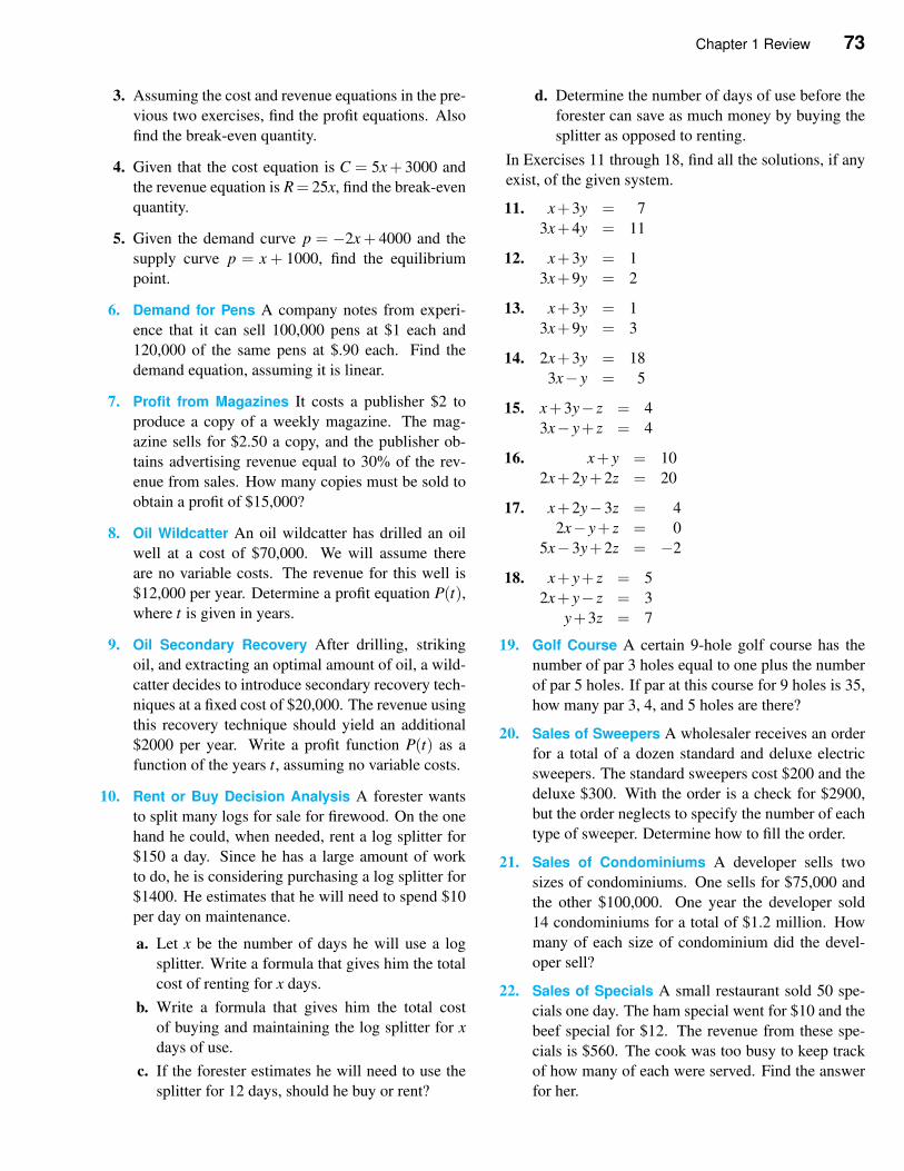
Chapter 1 Review 73
3. Assuming the cost and revenue equations in the pre-
vious two exercises, find the profit equations. Also
find the break-even quantity.
4. Given that the cost equation is C = 5x+ 3000 and
the revenue equation is R = 25x, find the break-even
quantity.
5. Given the demand curve p = −2x+ 4000 and the
supply curve p = x + 1000, find the equilibrium
point.
6. Demand for Pens A company notes from experi-
ence that it can sell 100,000 pens at $1 each and
120,000 of the same pens at $.90 each. Find the
demand equation, assuming it is linear.
7. Profit from Magazines It costs a publisher $2 to
produce a copy of a weekly magazine. The mag-
azine sells for $2.50 a copy, and the publisher ob-
tains advertising revenue equal to 30% of the rev-
enue from sales. How many copies must be sold to
obtain a profit of $15,000?
8. Oil Wildcatter An oil wildcatter has drilled an oil
well at a cost of $70,000. We will assume there
are no variable costs. The revenue for this well is
$12,000 per year. Determine a profit equation P(t),where t is given in years.
9. Oil Secondary Recovery After drilling, striking
oil, and extracting an optimal amount of oil, a wild-
catter decides to introduce secondary recovery tech-
niques at a fixed cost of $20,000. The revenue using
this recovery technique should yield an additional
$2000 per year. Write a profit function P(t) as a
function of the years t, assuming no variable costs.
10. Rent or Buy Decision Analysis A forester wants
to split many logs for sale for firewood. On the one
hand he could, when needed, rent a log splitter for
$150 a day. Since he has a large amount of work
to do, he is considering purchasing a log splitter for
$1400. He estimates that he will need to spend $10
per day on maintenance.
a. Let x be the number of days he will use a log
splitter. Write a formula that gives him the total
cost of renting for x days.
b. Write a formula that gives him the total cost
of buying and maintaining the log splitter for x
days of use.
c. If the forester estimates he will need to use the
splitter for 12 days, should he buy or rent?
d. Determine the number of days of use before the
forester can save as much money by buying the
splitter as opposed to renting.
In Exercises 11 through 18, find all the solutions, if any
exist, of the given system.
11. x+3y = 7
3x+4y = 11
12. x+3y = 1
3x+9y = 2
13. x+3y = 1
3x+9y = 3
14. 2x+3y = 18
3x− y = 5
15. x+3y− z = 4
3x− y+ z = 4
16. x+ y = 10
2x+2y+2z = 20
17. x+2y−3z = 4
2x− y+ z = 0
5x−3y+2z = −2
18. x+ y+ z = 5
2x+ y− z = 3
y+3z = 7
19. Golf Course A certain 9-hole golf course has the
number of par 3 holes equal to one plus the number
of par 5 holes. If par at this course for 9 holes is 35,
how many par 3, 4, and 5 holes are there?
20. Sales of Sweepers A wholesaler receives an order
for a total of a dozen standard and deluxe electric
sweepers. The standard sweepers cost $200 and the
deluxe $300. With the order is a check for $2900,
but the order neglects to specify the number of each
type of sweeper. Determine how to fill the order.
21. Sales of Condominiums A developer sells two
sizes of condominiums. One sells for $75,000 and
the other $100,000. One year the developer sold
14 condominiums for a total of $1.2 million. How
many of each size of condominium did the devel-
oper sell?
22. Sales of Specials A small restaurant sold 50 spe-
cials one day. The ham special went for $10 and the
beef special for $12. The revenue from these spe-
cials is $560. The cook was too busy to keep track
of how many of each were served. Find the answer
for her.
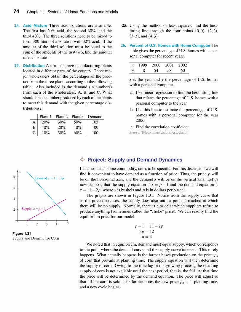
74 Chapter 1 Systems of Linear Equations and Models
23. Acid Mixture Three acid solutions are available.
The first has 20% acid, the second 30%, and the
third 40%. The three solutions need to be mixed to
form 300 liters of a solution with 32% acid. If the
amount of the third solution must be equal to the
sum of the amounts of the first two, find the amount
of each solution.
24. Distribution A firm has three manufacturing plants
located in different parts of the country. Three ma-
jor wholesalers obtain the percentages of the prod-
uct from the three plants according to the following
table. Also included is the demand (in numbers)
from each of the wholesalers, A, B, and C. What
should be the number produced by each of the plants
to meet this demand with the given percentage dis-
tributions?
Plant 1 Plant 2 Plant 3 Demand
A 20% 30% 50% 105
B 40% 20% 40% 100
C 10% 30% 60% 100
25. Using the method of least squares, find the best-
fitting line through the four points (0,0), (2,2),(3,2), and (4,3).
26. Percent of U.S. Homes with Home Computer The
table gives the percentage of U.S. homes with a per-
sonal computer for recent years.
x 1999 2000 2001 2002
y 48 54 58 60
x is the year and y the percentage of U.S. homes
with a personal computer.
a. Use linear regression to find the best-fitting line
that relates the percentage of U.S. homes with a
personal computer to the year.
b. Use this line to estimate the percentage of U.S.
homes with a personal computer for the year
2006.
c. Find the correlation coefficient.
Source: Telecommunications Association
✧ Project: Supply and Demand Dynamics
Let us consider some commodity, corn, to be specific. For this discussion we will
find it convenient to have demand as a function of price. Thus, the price p will
be on the horizontal axis, and the demand x will be on the vertical axis. Let us
now suppose that the supply equation is x = p− 1 and the demand equation is
x = 11−2p, where x is bushels and p is in dollars per bushel.
Figure 1.31
Supply and Demand for Corn
The graphs are shown in Figure 1.31. Notice from the supply curve that
as the price decreases, the supply does also until a point is reached at which
there will be no supply. Normally, there is a price at which suppliers refuse to
produce anything (sometimes called the “choke” price). We can readily find the
equilibrium price for our model:
p−1 = 11−2p
3p = 12
p = 4
We noted that in equilibrium, demand must equal supply, which corresponds
to the point where the demand curve and the supply curve intersect. This rarely
happens. What actually happens is the farmer bases production on the price pn
of corn that prevails at planting time. The supply equation will then determine
the supply of corn. Owing to the time lag in the growing process, the resulting
supply of corn is not available until the next period, that is, the fall. At that time
the price will be determined by the demand equation. The price will adjust so
that all the corn is sold. The farmer notes the new price pn+1 at planting time,
and a new cycle begins.
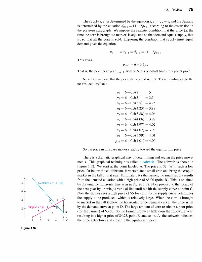
1.5 Review 75
The supply sn+1 is determined by the equation sn+1 = pn−1, and the demand
is determined by the equation dn+1 = 11− 2pn+1 according to the discussion in
the previous paragraph. We impose the realistic condition that the price (at the
time the corn is brought to market) is adjusted so that demand equals supply, that
is, so that all the corn is sold. Imposing the condition that supply must equal
demand gives the equation
pn−1 = sn+1 = dn+1 = 11−2pn+1
This gives
pn+1 = 6−0.5pn
That is, the price next year, pn+1, will be 6 less one-half times this year’s price.
Now let’s suppose that the price starts out at p0 = 2. Then rounding off to the
nearest cent we have
p1 = 6−0.5(2) = 5
p2 = 6−0.5(5) = 3.5
p3 = 6−0.5(3.5) = 4.25
p4 = 6−0.5(4.25) = 3.88
p5 = 6−0.5(3.88) = 4.06
p6 = 6−0.5(4.06) = 3.97
p7 = 6−0.5(3.97) = 4.02
p8 = 6−0.5(4.02) = 3.99
p9 = 6−0.5(3.99) = 4.01
p10 = 6−0.5(4.01) = 4.00
So the price in this case moves steadily toward the equilibrium price.
There is a dramatic graphical way of determining and seeing the price move-
ments. This graphical technique is called a cobweb. The cobweb is shown in
Figure 1.32. We start at the point labeled A. The price is $2. With such a low
price, far below the equilibrium, farmers plant a small crop and bring the crop to
market in the fall of that year. Fortunately for the farmer, the small supply results
from the demand equation with a high price of $5.00 (point B). This is obtained
by drawing the horizontal line seen in Figure 1.32. Now proceed to the spring of
the next year by drawing a vertical line until we hit the supply curve at point C.
Now the farmer sees a high price of $5 for corn, so the supply curve determines
the supply to be produced, which is relatively large. When the corn is brought
to market in the fall (follow the horizontal to the demand curve), the price is set
by the demand curve at point D. The large amount of corn results in a poor price
(for the farmer) of $3.50. So the farmer produces little corn the following year,
resulting in a higher price of $4.25, point E, and so on. As the cobweb indicates,
the price gets closer and closer to the equilibrium price.
Figure 1.32
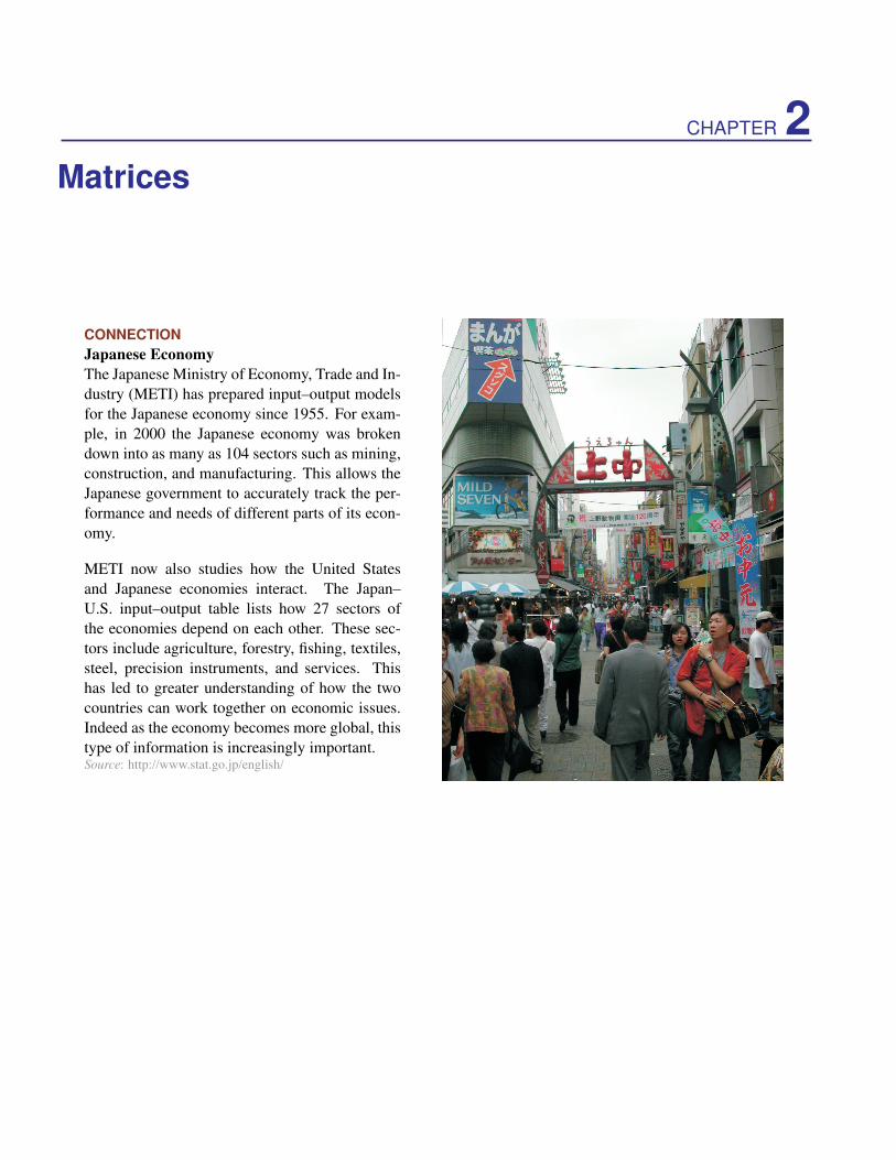
CHAPTER 2Matrices
CONNECTION
Japanese Economy
The Japanese Ministry of Economy, Trade and In-
dustry (METI) has prepared input–output models
for the Japanese economy since 1955. For exam-
ple, in 2000 the Japanese economy was broken
down into as many as 104 sectors such as mining,
construction, and manufacturing. This allows the
Japanese government to accurately track the per-
formance and needs of different parts of its econ-
omy.
METI now also studies how the United States
and Japanese economies interact. The Japan–
U.S. input–output table lists how 27 sectors of
the economies depend on each other. These sec-
tors include agriculture, forestry, fishing, textiles,
steel, precision instruments, and services. This
has led to greater understanding of how the two
countries can work together on economic issues.
Indeed as the economy becomes more global, this
type of information is increasingly important.Source: http://www.stat.go.jp/english/
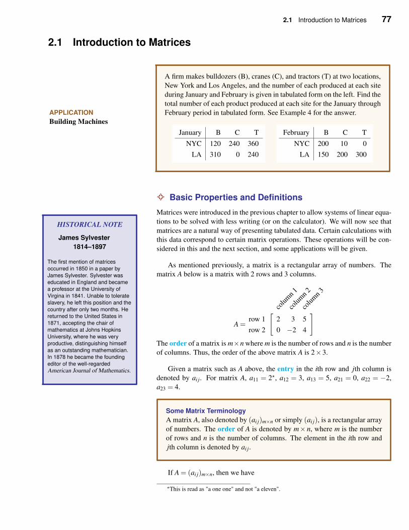
2.1 Introduction to Matrices 77
2.1 Introduction to Matrices
APPLICATION
Building Machines
A firm makes bulldozers (B), cranes (C), and tractors (T) at two locations,
New York and Los Angeles, and the number of each produced at each site
during January and February is given in tabulated form on the left. Find the
total number of each product produced at each site for the January through
February period in tabulated form. See Example 4 for the answer.
January B C T
NYC 120 240 360
LA 310 0 240
February B C T
NYC 200 10 0
LA 150 200 300
✧ Basic Properties and Definitions
Matrices were introduced in the previous chapter to allow systems of linear equa-
tions to be solved with less writing (or on the calculator). We will now see that
matrices are a natural way of presenting tabulated data. Certain calculations with
this data correspond to certain matrix operations. These operations will be con-
sidered in this and the next section, and some applications will be given.
As mentioned previously, a matrix is a rectangular array of numbers. The
matrix A below is a matrix with 2 rows and 3 columns.
HISTORICAL NOTE
James Sylvester
1814–1897
The first mention of matrices
occurred in 1850 in a paper by
James Sylvester. Sylvester was
educated in England and became
a professor at the University of
Virgina in 1841. Unable to tolerate
slavery, he left this position and the
country after only two months. He
returned to the United States in
1871, accepting the chair of
mathematics at Johns Hopkins
University, where he was very
productive, distinguishing himself
as an outstanding mathematician.
In 1878 he became the founding
editor of the well-regarded
American Journal of Mathematics.
A =
[co
lum
n1
colu
mn
2
colu
mn
3
row 1 2 3 5
row 2 0 −2 4
]
The order of a matrix is m×n where m is the number of rows and n is the number
of columns. Thus, the order of the above matrix A is 2×3.
Given a matrix such as A above, the entry in the ith row and jth column is
denoted by ai j. For matrix A, a11 = 2⋆, a12 = 3, a13 = 5, a21 = 0, a22 = −2,
a23 = 4.
Some Matrix Terminology
A matrix A, also denoted by (ai j)m×n or simply (ai j), is a rectangular array
of numbers. The order of A is denoted by m× n, where m is the number
of rows and n is the number of columns. The element in the ith row and
jth column is denoted by ai j.
If A = (ai j)m×n, then we have
⋆This is read as "a one one" and not "a eleven".
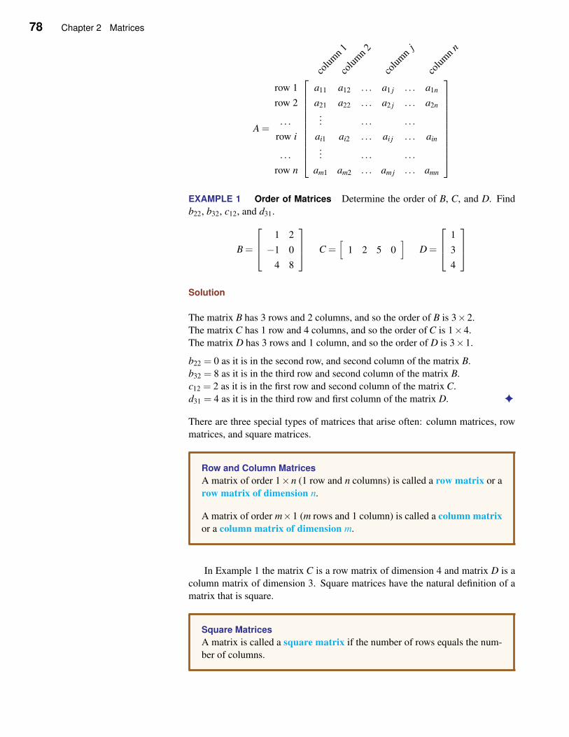
78 Chapter 2 Matrices
A =
colu
mn
1
colu
mn
2
colu
mn
j
colu
mn
n
row 1 a11 a12 . . . a1 j . . . a1n
row 2 a21 a22 . . . a2 j . . . a2n
. . .... . . . . . .
row i ai1 ai2 . . . ai j . . . ain
. . .... . . . . . .
row n am1 am2 . . . am j . . . amn
EXAMPLE 1 Order of Matrices Determine the order of B, C, and D. Find
b22, b32, c12, and d31.
B =
1 2
−1 0
4 8
C =
[
1 2 5 0]
D =
1
3
4
Solution
The matrix B has 3 rows and 2 columns, and so the order of B is 3×2.
The matrix C has 1 row and 4 columns, and so the order of C is 1×4.
The matrix D has 3 rows and 1 column, and so the order of D is 3×1.
b22 = 0 as it is in the second row, and second column of the matrix B.
b32 = 8 as it is in the third row and second column of the matrix B.
c12 = 2 as it is in the first row and second column of the matrix C.
d31 = 4 as it is in the third row and first column of the matrix D. ✦
There are three special types of matrices that arise often: column matrices, row
matrices, and square matrices.
Row and Column Matrices
A matrix of order 1×n (1 row and n columns) is called a row matrix or a
row matrix of dimension n.
A matrix of order m×1 (m rows and 1 column) is called a column matrix
or a column matrix of dimension m.
In Example 1 the matrix C is a row matrix of dimension 4 and matrix D is a
column matrix of dimension 3. Square matrices have the natural definition of a
matrix that is square.
Square Matrices
A matrix is called a square matrix if the number of rows equals the num-
ber of columns.
2.1 Introduction to Matrices 79
Naturally we need to know when two matrices are equal. Two matrices are
equal when they are absolutely identical. The following definition says just that.
Equality of Matrices
Two matrices are equal if they have the same order and all corresponding
entries are equal.
For example, none of the matrices below are equal. Remember, first the
matrices must be the same order and then all corresponding entries must be equal.
[
1 2
3 4
] [
1 3
2 4
] [
1 2 0
3 4 0
]
1 2
3 4
0 0
EXAMPLE 2 Equal Matrices Find x, y, and z, such that
[
1 2 x
3 0 5
]
=
[
1 2 4
y 0 z
]
Solution Since both matrices have order 2×3, equality is possible. Setting the
corresponding entries equal gives x = 4, y = 3, and z = 5. ✦
We now state three fundamental operations on matrices.
Multiplication of a Matrix by a Number
If c is a number and A is a matrix, then the matrix cA is the matrix obtained
by multiplying every entry in A by c.
REMARK: The number c can be referred to as a scalar to distinguish it from
a 1× 1 matrix. Then the operation defined above would be referred to as scalar
multiplication
Addition and Subtraction of Matrices
Two matrices of the same order can be added (or subtracted) to obtain
another matrix of the same order by adding (or subtracting) corresponding
entries.
The Transpose of a Matrix
If A is an m× n matrix with elements ai j, then the transpose of A is the
n×m matrix AT with elements a ji.
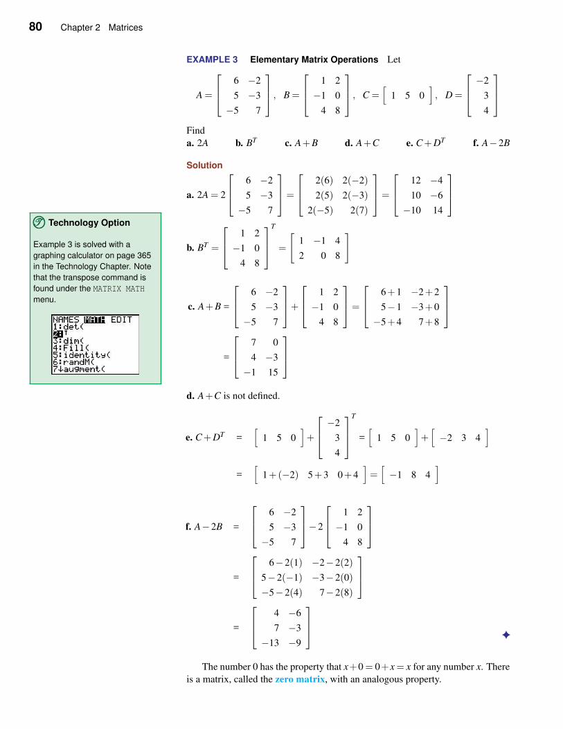
80 Chapter 2 Matrices
EXAMPLE 3 Elementary Matrix Operations Let
A =
6 −2
5 −3
−5 7
, B =
1 2
−1 0
4 8
, C =
[
1 5 0]
, D =
−2
3
4
Find
a. 2A b. BT c. A+B d. A+C e. C+DT f. A−2B
Solution
TTT©©© Technology Option
Example 3 is solved with a
graphing calculator on page 365
in the Technology Chapter. Note
that the transpose command is
found under the MATRIX MATH
menu.
a. 2A = 2
6 −2
5 −3
−5 7
=
2(6) 2(−2)
2(5) 2(−3)
2(−5) 2(7)
=
12 −4
10 −6
−10 14
b. BT =
1 2
−1 0
4 8
T
=
[
1 −1 4
2 0 8
]
c. A+B =
6 −2
5 −3
−5 7
+
1 2
−1 0
4 8
=
6+1 −2+2
5−1 −3+0
−5+4 7+8
=
7 0
4 −3
−1 15
d. A+C is not defined.
e. C+DT =[
1 5 0]
+
−2
3
4
T
=[
1 5 0]
+[
−2 3 4]
=[
1+(−2) 5+3 0+4]
=[
−1 8 4]
f. A−2B =
6 −2
5 −3
−5 7
−2
1 2
−1 0
4 8
=
6−2(1) −2−2(2)
5−2(−1) −3−2(0)
−5−2(4) 7−2(8)
=
4 −6
7 −3
−13 −9
✦
The number 0 has the property that x+0 = 0+x = x for any number x. There
is a matrix, called the zero matrix, with an analogous property.
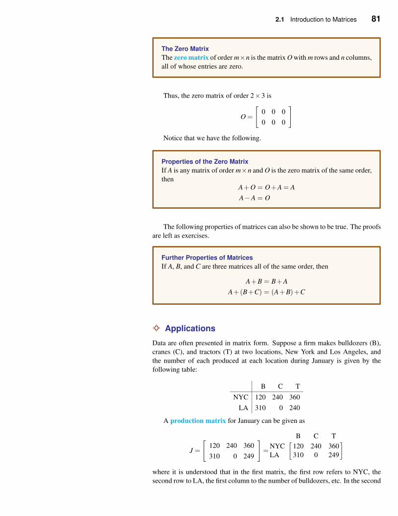
2.1 Introduction to Matrices 81
The Zero Matrix
The zero matrix of order m×n is the matrix O with m rows and n columns,
all of whose entries are zero.
Thus, the zero matrix of order 2×3 is
O =
[
0 0 0
0 0 0
]
Notice that we have the following.
Properties of the Zero Matrix
If A is any matrix of order m×n and O is the zero matrix of the same order,
thenA+O = O+A = A
A−A = O
The following properties of matrices can also be shown to be true. The proofs
are left as exercises.
Further Properties of Matrices
If A, B, and C are three matrices all of the same order, then
A+B = B+A
A+(B+C) = (A+B)+C
✧ Applications
Data are often presented in matrix form. Suppose a firm makes bulldozers (B),
cranes (C), and tractors (T) at two locations, New York and Los Angeles, and
the number of each produced at each location during January is given by the
following table:
B C T
NYC 120 240 360
LA 310 0 240
A production matrix for January can be given as
J =
[
120 240 360
310 0 249
]
=
[B C T
NYC 120 240 360
LA 310 0 249
]
where it is understood that in the first matrix, the first row refers to NYC, the
second row to LA, the first column to the number of bulldozers, etc. In the second
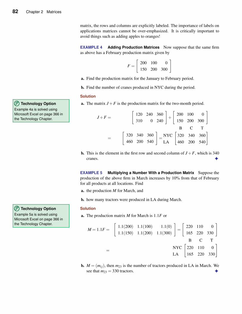
82 Chapter 2 Matrices
matrix, the rows and columns are explicitly labeled. The importance of labels on
applications matrices cannot be over-emphasized. It is critically important to
avoid things such as adding apples to oranges!
EXAMPLE 4 Adding Production Matrices Now suppose that the same firm
as above has a February production matrix given by
F =
[
200 100 0
150 200 300
]
a. Find the production matrix for the January to February period.
b. Find the number of cranes produced in NYC during the period.
Solution
a. The matrix J+F is the production matrix for the two-month period.TTT©©© Technology Option
Example 4a is solved using
Microsoft Excel on page 366 in
the Technology Chapter. J+F =
[
120 240 360
310 0 240
]
+
[
200 100 0
150 200 300
]
=
[
320 340 360
460 200 540
]
=
[B C T
NYC 320 340 360
LA 460 200 540
]
b. This is the element in the first row and second column of J+F , which is 340
cranes. ✦
EXAMPLE 5 Multiplying a Number With a Production Matrix Suppose the
production of the above firm in March increases by 10% from that of February
for all products at all locations. Find
a. the production M for March, and
b. how many tractors were produced in LA during March.
Solution
a. The production matrix M for March is 1.1F or
TTT©©© Technology Option
Example 5a is solved using
Microsoft Excel on page 366 in
the Technology Chapter.
M = 1.1F =
[
1.1(200) 1.1(100) 1.1(0)
1.1(150) 1.1(200) 1.1(300)
]
=
[
220 110 0
165 220 330
]
=
[B C T
NYC 220 110 0
LA 165 220 330
]
b. M = (mi j), then m23 is the number of tractors produced in LA in March. We
see that m23 = 330 tractors. ✦
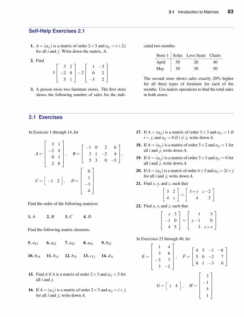
2.1 Introduction to Matrices 83
Self-Help Exercises 2.1
1. A = (ai j) is a matrix of order 2×3 and ai j = i+2 j
for all i and j. Write down the matrix, A.
2. Find
3
3 2
−2 0
5 1
−2
1 −3
0 2
−3 2
3. A person owns two furniture stores. The first store
shows the following number of sales for the indi-
cated two months:
Store 1 Sofas Love Seats Chairs
April 30 20 40
May 30 30 50
The second store shows sales exactly 20% higher
for all three types of furniture for each of the
months. Use matrix operations to find the total sales
in both stores.
2.1 Exercises
In Exercise 1 through 14, let
A =
3 1
−2 4
0 3
2 8
, B =
−1 0 2 6
3 1 −2 4
5 3 0 −5
,
C =[
−1 2]
, D =
0
1
−3
4
Find the order of the following matrices.
1. A 2. B 3. C 4. D
Find the following matrix elements.
5. a12 6. a21 7. a42 8. a41 9. b23
10. b34 11. b14 12. b33 13. c12 14. d31
15. Find A if A is a matrix of order 2×3 and ai j = 5 for
all i and j.
16. If A = (ai j) is a matrix of order 2×3 and ai j = i+ j
for all i and j, write down A.
17. If A = (ai j) is a matrix of order 3×3 and ai j = 1 if
i = j, and ai j = 0 if i 6= j, write down A.
18. If A = (ai j) is a matrix of order 3×2 and ai j = 1 for
all i and j, write down A.
19. If A = (ai j) is a matrix of order 3×3 and ai j = 0 for
all i and j, write down A.
20. If A= (ai j) is a matrix of order 4×3 and ai j = 2i+ j
for all i and j, write down A.
21. Find x, y, and z, such that[
3 2
4 x
]
=
[
3+ y z−2
4 3
]
22. Find x, y, and z, such that
x 3
−1 0
4 5
=
1 3
y−1 0
3 z+ x
In Exercises 23 through 40, let
E =
1 4
3 6
−3 7
3 −2
, F =
4 3 −1 −6
5 0 −2 7
8 1 −3 0
G =[
1 4]
, H =
3
−1
5
1
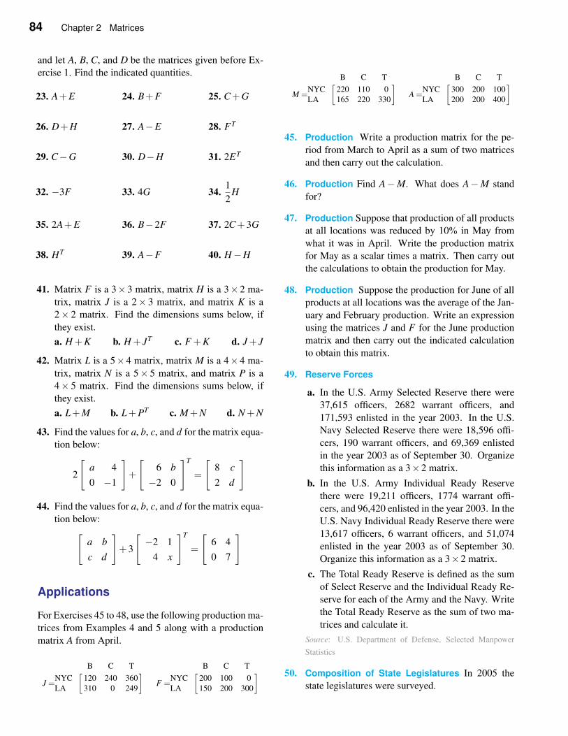
84 Chapter 2 Matrices
and let A, B, C, and D be the matrices given before Ex-
ercise 1. Find the indicated quantities.
23. A+E 24. B+F 25. C+G
26. D+H 27. A−E 28. FT
29. C−G 30. D−H 31. 2ET
32. −3F 33. 4G 34.1
2H
35. 2A+E 36. B−2F 37. 2C+3G
38. HT 39. A−F 40. H−H
41. Matrix F is a 3×3 matrix, matrix H is a 3×2 ma-
trix, matrix J is a 2× 3 matrix, and matrix K is a
2× 2 matrix. Find the dimensions sums below, if
they exist.
a. H +K b. H + JT c. F +K d. J+ J
42. Matrix L is a 5× 4 matrix, matrix M is a 4× 4 ma-
trix, matrix N is a 5× 5 matrix, and matrix P is a
4× 5 matrix. Find the dimensions sums below, if
they exist.
a. L+M b. L+PT c. M+N d. N +N
43. Find the values for a, b, c, and d for the matrix equa-
tion below:
2
[
a 4
0 −1
]
+
[
6 b
−2 0
]T
=
[
8 c
2 d
]
44. Find the values for a, b, c, and d for the matrix equa-
tion below:
[
a b
c d
]
+3
[
−2 1
4 x
]T
=
[
6 4
0 7
]
Applications
For Exercises 45 to 48, use the following production ma-
trices from Examples 4 and 5 along with a production
matrix A from April.
J =
[B C T
NYC 120 240 360
LA 310 0 249
]
F =
[B C T
NYC 200 100 0
LA 150 200 300
]
M =
[B C T
NYC 220 110 0
LA 165 220 330
]
A =
[B C T
NYC 300 200 100
LA 200 200 400
]
45. Production Write a production matrix for the pe-
riod from March to April as a sum of two matrices
and then carry out the calculation.
46. Production Find A−M. What does A−M stand
for?
47. Production Suppose that production of all products
at all locations was reduced by 10% in May from
what it was in April. Write the production matrix
for May as a scalar times a matrix. Then carry out
the calculations to obtain the production for May.
48. Production Suppose the production for June of all
products at all locations was the average of the Jan-
uary and February production. Write an expression
using the matrices J and F for the June production
matrix and then carry out the indicated calculation
to obtain this matrix.
49. Reserve Forces
a. In the U.S. Army Selected Reserve there were
37,615 officers, 2682 warrant officers, and
171,593 enlisted in the year 2003. In the U.S.
Navy Selected Reserve there were 18,596 offi-
cers, 190 warrant officers, and 69,369 enlisted
in the year 2003 as of September 30. Organize
this information as a 3×2 matrix.
b. In the U.S. Army Individual Ready Reserve
there were 19,211 officers, 1774 warrant offi-
cers, and 96,420 enlisted in the year 2003. In the
U.S. Navy Individual Ready Reserve there were
13,617 officers, 6 warrant officers, and 51,074
enlisted in the year 2003 as of September 30.
Organize this information as a 3×2 matrix.
c. The Total Ready Reserve is defined as the sum
of Select Reserve and the Individual Ready Re-
serve for each of the Army and the Navy. Write
the Total Ready Reserve as the sum of two ma-
trices and calculate it.
Source: U.S. Department of Defense, Selected Manpower
Statistics
50. Composition of State Legislatures In 2005 the
state legislatures were surveyed.
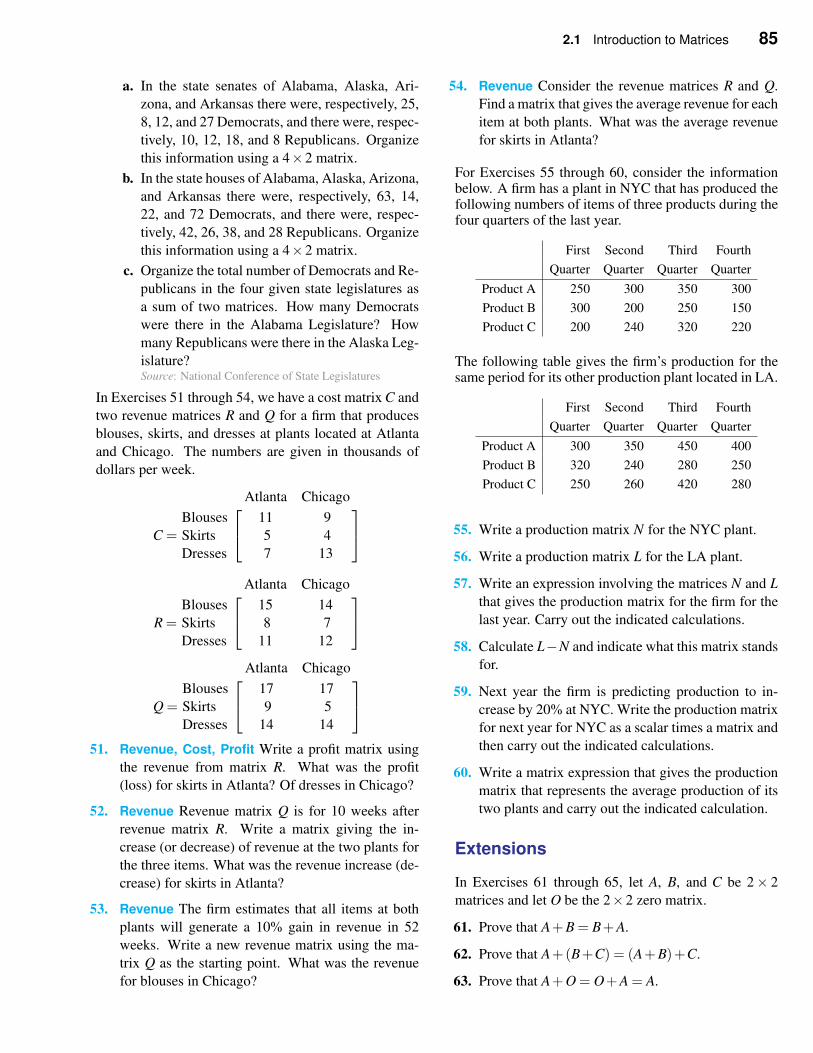
2.1 Introduction to Matrices 85
a. In the state senates of Alabama, Alaska, Ari-
zona, and Arkansas there were, respectively, 25,
8, 12, and 27 Democrats, and there were, respec-
tively, 10, 12, 18, and 8 Republicans. Organize
this information using a 4×2 matrix.
b. In the state houses of Alabama, Alaska, Arizona,
and Arkansas there were, respectively, 63, 14,
22, and 72 Democrats, and there were, respec-
tively, 42, 26, 38, and 28 Republicans. Organize
this information using a 4×2 matrix.
c. Organize the total number of Democrats and Re-
publicans in the four given state legislatures as
a sum of two matrices. How many Democrats
were there in the Alabama Legislature? How
many Republicans were there in the Alaska Leg-
islature?Source: National Conference of State Legislatures
In Exercises 51 through 54, we have a cost matrix C and
two revenue matrices R and Q for a firm that produces
blouses, skirts, and dresses at plants located at Atlanta
and Chicago. The numbers are given in thousands of
dollars per week.
C =
Atlanta Chicago
Blouses 11 9
Skirts 5 4
Dresses 7 13
R =
Atlanta Chicago
Blouses 15 14
Skirts 8 7
Dresses 11 12
Q =
Atlanta Chicago
Blouses 17 17
Skirts 9 5
Dresses 14 14
51. Revenue, Cost, Profit Write a profit matrix using
the revenue from matrix R. What was the profit
(loss) for skirts in Atlanta? Of dresses in Chicago?
52. Revenue Revenue matrix Q is for 10 weeks after
revenue matrix R. Write a matrix giving the in-
crease (or decrease) of revenue at the two plants for
the three items. What was the revenue increase (de-
crease) for skirts in Atlanta?
53. Revenue The firm estimates that all items at both
plants will generate a 10% gain in revenue in 52
weeks. Write a new revenue matrix using the ma-
trix Q as the starting point. What was the revenue
for blouses in Chicago?
54. Revenue Consider the revenue matrices R and Q.
Find a matrix that gives the average revenue for each
item at both plants. What was the average revenue
for skirts in Atlanta?
For Exercises 55 through 60, consider the informationbelow. A firm has a plant in NYC that has produced thefollowing numbers of items of three products during thefour quarters of the last year.
First Second Third Fourth
Quarter Quarter Quarter Quarter
Product A 250 300 350 300
Product B 300 200 250 150
Product C 200 240 320 220
The following table gives the firm’s production for thesame period for its other production plant located in LA.
First Second Third Fourth
Quarter Quarter Quarter Quarter
Product A 300 350 450 400
Product B 320 240 280 250
Product C 250 260 420 280
55. Write a production matrix N for the NYC plant.
56. Write a production matrix L for the LA plant.
57. Write an expression involving the matrices N and L
that gives the production matrix for the firm for the
last year. Carry out the indicated calculations.
58. Calculate L−N and indicate what this matrix stands
for.
59. Next year the firm is predicting production to in-
crease by 20% at NYC. Write the production matrix
for next year for NYC as a scalar times a matrix and
then carry out the indicated calculations.
60. Write a matrix expression that gives the production
matrix that represents the average production of its
two plants and carry out the indicated calculation.
Extensions
In Exercises 61 through 65, let A, B, and C be 2× 2
matrices and let O be the 2×2 zero matrix.
61. Prove that A+B = B+A.
62. Prove that A+(B+C) = (A+B)+C.
63. Prove that A+O = O+A = A.
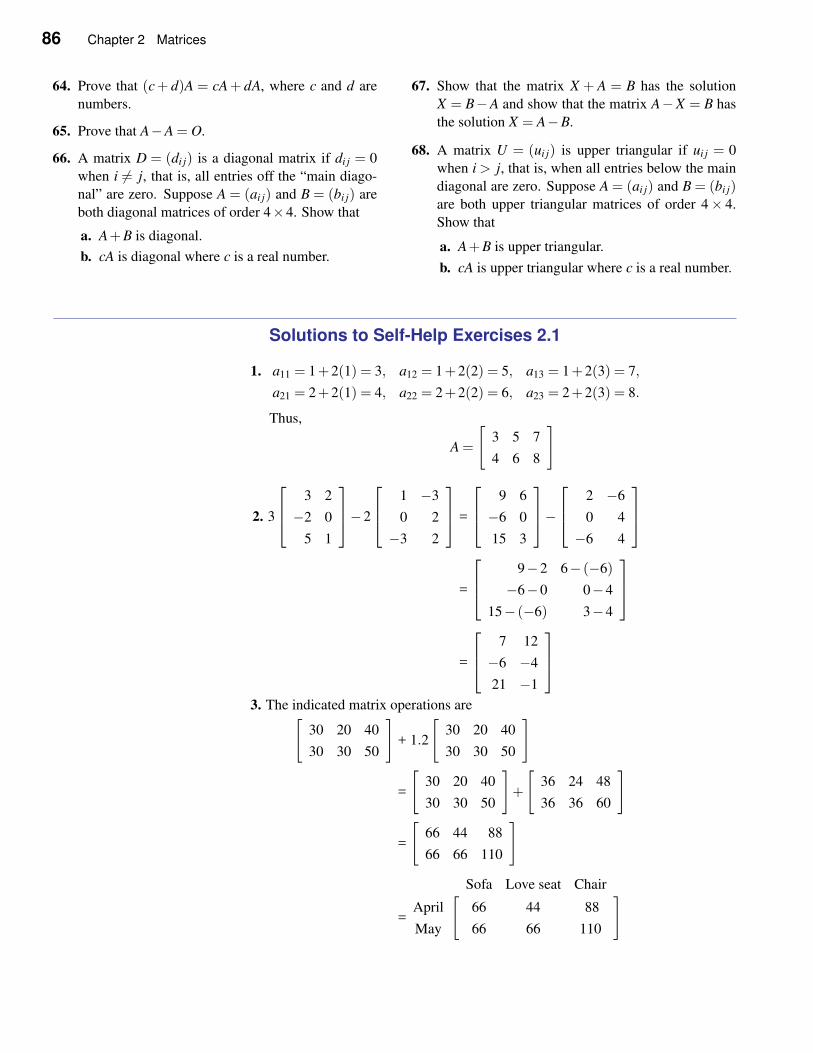
86 Chapter 2 Matrices
64. Prove that (c+ d)A = cA+ dA, where c and d are
numbers.
65. Prove that A−A = O.
66. A matrix D = (di j) is a diagonal matrix if di j = 0
when i 6= j, that is, all entries off the “main diago-
nal” are zero. Suppose A = (ai j) and B = (bi j) are
both diagonal matrices of order 4×4. Show that
a. A+B is diagonal.
b. cA is diagonal where c is a real number.
67. Show that the matrix X + A = B has the solution
X = B−A and show that the matrix A−X = B has
the solution X = A−B.
68. A matrix U = (ui j) is upper triangular if ui j = 0
when i > j, that is, when all entries below the main
diagonal are zero. Suppose A = (ai j) and B = (bi j)are both upper triangular matrices of order 4× 4.
Show that
a. A+B is upper triangular.
b. cA is upper triangular where c is a real number.
Solutions to Self-Help Exercises 2.1
1. a11 = 1+2(1) = 3, a12 = 1+2(2) = 5, a13 = 1+2(3) = 7,
a21 = 2+2(1) = 4, a22 = 2+2(2) = 6, a23 = 2+2(3) = 8.
Thus,
A =
[
3 5 7
4 6 8
]
2. 3
3 2
−2 0
5 1
−2
1 −3
0 2
−3 2
=
9 6
−6 0
15 3
−
2 −6
0 4
−6 4
=
9−2 6− (−6)
−6−0 0−4
15− (−6) 3−4
=
7 12
−6 −4
21 −1
3. The indicated matrix operations are[
30 20 40
30 30 50
]
+ 1.2
[
30 20 40
30 30 50
]
=
[
30 20 40
30 30 50
]
+
[
36 24 48
36 36 60
]
=
[
66 44 88
66 66 110
]
=
[Sofa Love seat Chair
April 66 44 88
May 66 66 110
]
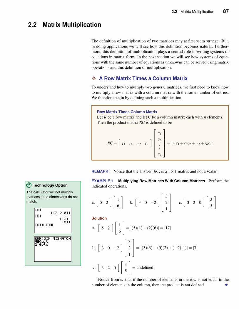
2.2 Matrix Multiplication 87
2.2 Matrix Multiplication
The definition of multiplication of two matrices may at first seem strange. But,
in doing applications we will see how this definition becomes natural. Further-
more, this definition of multiplication plays a central role in writing systems of
equations in matrix form. In the next section we will see how systems of equa-
tions with the same number of equations as unknowns can be solved using matrix
operations and this definition of multiplication.
✧ A Row Matrix Times a Column Matrix
To understand how to multiply two general matrices, we first need to know how
to multiply a row matrix with a column matrix with the same number of entries.
We therefore begin by defining such a multiplication.
Row Matrix Times Column Matrix
Let R be a row matrix and let C be a column matrix each with n elements.
Then the product matrix RC is defined to be
RC =[
r1 r2 · · · rn
]
c1
c2
...
cn
= [r1c1 + r2c2 + · · ·+ rncn]
REMARK: Notice that the answer, RC, is a 1×1 matrix and not a scalar.
EXAMPLE 1 Multiplying Row Matrices With Column Matrices Perform the
indicated operations.
a.[
5 2][
1
6
]
b.[
3 0 −2]
3
2
1
c.
[
3 2 0][
3
5
]
TTT©©© Technology Option
The calculator will not multiply
matrices if the dimensions do not
match.
Solution
a.[
5 2][
1
6
]
= [(5)(1)+(2)(6)] = [17]
b.[
3 0 −2]
3
2
1
= [(3)(3)+(0)(2)+(−2)(1)] = [7]
c.[
3 2 0][
3
5
]
= undefined
Notice from c. that if the number of elements in the row is not equal to the
number of elements in the column, then the product is not defined ✦
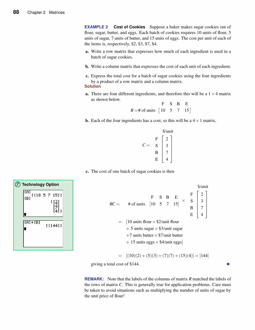
88 Chapter 2 Matrices
EXAMPLE 2 Cost of Cookies Suppose a baker makes sugar cookies out of
flour, sugar, butter, and eggs. Each batch of cookies requires 10 units of flour, 5
units of sugar, 7 units of butter, and 15 units of eggs. The cost per unit of each of
the items is, respectively, $2, $3, $7, $4.
a. Write a row matrix that expresses how much of each ingredient is used in a
batch of sugar cookies.
b. Write a column matrix that expresses the cost of each unit of each ingredient.
c. Express the total cost for a batch of sugar cookies using the four ingredients
by a product of a row matrix and a column matrix.Solution
a. There are four different ingredients, and therefore this will be a 1×4 matrix
as shown below.
R =[
F S B E
# of units 10 5 7 15]
b. Each of the four ingredients has a cost, so this will be a 4×1 matrix,
C =
$/unit
F
S
B
E
2
3
7
4
c. The cost of one batch of sugar cookies is then
TTT©©© Technology Option
RC =
F S B E
# of units [10 5 7 15]×
$/unit
F
S
B
E
2
3
7
4
= [10 units flour×$2/unit flour
+ 5 units sugar×$3/unit sugar
+7 units butter×$7/unit butter
+ 15 units eggs×$4/unit eggs]
= [(10)(2)+(5)(3)+(7)(7)+(15)(4)] = [144]
giving a total cost of $144. ✦
REMARK: Note that the labels of the columns of matrix R matched the labels of
the rows of matrix C. This is generally true for application problems. Care must
be taken to avoid situations such as multiplying the number of units of sugar by
the unit price of flour!
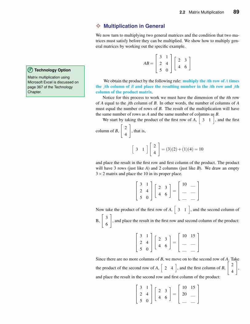
2.2 Matrix Multiplication 89
✧ Multiplication in General
We now turn to multiplying two general matrices and the condition that two ma-
trices must satisfy before they can be multiplied. We show how to multiply gen-
eral matrices by working out the specific example.
AB =
3 1
2 4
5 0
[
2 3
4 6
]
We obtain the product by the following rule: multiply the ith row of A times
TTT©©© Technology Option
Matrix multiplication using
Microsoft Excel is discussed on
page 367 of the Technology
Chapter.
the jth column of B and place the resulting number in the ith row and jth
column of the product matrix.
Notice for this process to work we must have the dimension of the ith row
of A equal to the jth column of B. In other words, the number of columns of A
must equal the number of rows of B. The result of the multiplication will have
the same number of rows as A and the same number of columns as B.
We start by taking the product of the first row of A,[
3 1]
, and the first
column of B,
[
2
4
]
, that is,
[
3 1][
2
4
]
= (3)(2)+(1)(4) = 10
and place the result in the first row and first column of the product. The product
will have 3 rows (just like A) and 2 columns (just like B). We draw an empty
3×2 matrix and place the 10 in its proper place.
3 1
2 4
5 0
[
2 3
4 6
]
=
10
Now take the product of the first row of A,[
3 1]
, and the second column of
B,
[
3
6
]
, and place the result in the first row and second column of the product:
3 1
2 4
5 0
[
2 3
4 6
]
=
10 15
Since there are no more columns of B, we move on to the second row of A. Take
the product of the second row of A,[
2 4]
, and the first column of B,
[
2
4
]
,
and place the result in the second row and first column of the product:
3 1
2 4
5 0
[
2 3
4 6
]
=
10 15
20
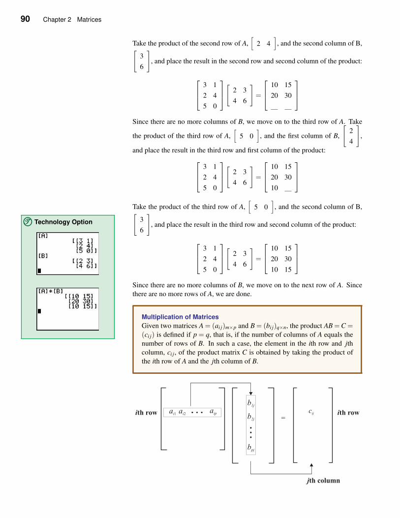
90 Chapter 2 Matrices
Take the product of the second row of A,[
2 4]
, and the second column of B,[
3
6
]
, and place the result in the second row and second column of the product:
3 1
2 4
5 0
[
2 3
4 6
]
=
10 15
20 30
Since there are no more columns of B, we move on to the third row of A. Take
the product of the third row of A,[
5 0]
, and the first column of B,
[
2
4
]
,
and place the result in the third row and first column of the product:
3 1
2 4
5 0
[
2 3
4 6
]
=
10 15
20 30
10
Take the product of the third row of A,[
5 0]
, and the second column of B,[
3
6
]
, and place the result in the third row and second column of the product:TTT©©© Technology Option
3 1
2 4
5 0
[
2 3
4 6
]
=
10 15
20 30
10 15
Since there are no more columns of B, we move on to the next row of A. Since
there are no more rows of A, we are done.
Multiplication of Matrices
Given two matrices A = (ai j)m×p and B = (bi j)q×n, the product AB =C =(ci j) is defined if p = q, that is, if the number of columns of A equals the
number of rows of B. In such a case, the element in the ith row and jth
column, ci j, of the product matrix C is obtained by taking the product of
the ith row of A and the jth column of B.
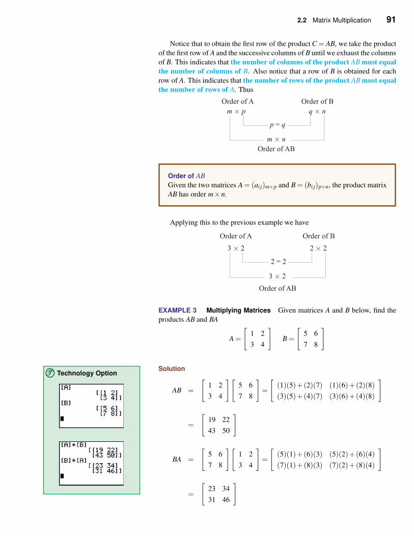
2.2 Matrix Multiplication 91
Notice that to obtain the first row of the product C = AB, we take the product
of the first row of A and the successive columns of B until we exhaust the columns
of B. This indicates that the number of columns of the product AB must equal
the number of columns of B. Also notice that a row of B is obtained for each
row of A. This indicates that the number of rows of the product AB must equal
the number of rows of A. Thus
Order of AB
Given the two matrices A = (ai j)m×p and B = (bi j)p×n, the product matrix
AB has order m×n.
Applying this to the previous example we have
EXAMPLE 3 Multiplying Matrices Given matrices A and B below, find the
products AB and BA
A =
[
1 2
3 4
]
B =
[
5 6
7 8
]
SolutionTTT©©© Technology Option
AB =
[
1 2
3 4
][
5 6
7 8
]
=
[
(1)(5)+(2)(7) (1)(6)+(2)(8)
(3)(5)+(4)(7) (3)(6)+(4)(8)
]
=
[
19 22
43 50
]
BA =
[
5 6
7 8
][
1 2
3 4
]
=
[
(5)(1)+(6)(3) (5)(2)+(6)(4)
(7)(1)+(8)(3) (7)(2)+(8)(4)
]
=
[
23 34
31 46
]
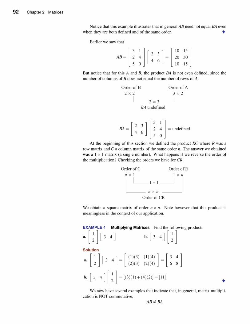
92 Chapter 2 Matrices
Notice that this example illustrates that in general AB need not equal BA even
when they are both defined and of the same order. ✦
Earlier we saw that
AB =
3 1
2 4
5 0
[
2 3
4 6
]
=
10 15
20 30
10 15
But notice that for this A and B, the product BA is not even defined, since the
number of columns of B does not equal the number of rows of A.
BA =
[
2 3
4 6
]
3 1
2 4
5 0
= undefined
At the beginning of this section we defined the product RC where R was a
row matrix and C a column matrix of the same order n. The answer we obtained
was a 1× 1 matrix (a single number). What happens if we reverse the order of
the multiplication? Checking the orders we have for CR,
We obtain a square matrix of order n× n. Note however that this product is
meaningless in the context of our application.
EXAMPLE 4 Multiplying Matrices Find the following products
a.
[
1
2
][
3 4]
b.[
3 4][
1
2
]
Solution
a.
[
1
2
][
3 4]
=
[
(1)(3) (1)(4)
(2)(3) (2)(4)
]
=
[
3 4
6 8
]
b.[
3 4][
1
2
]
= [(3)(1)+(4)(2)] = [11]✦
We now have several examples that indicate that, in general, matrix multipli-
cation is NOT commutative,
AB 6= BA
2.2 Matrix Multiplication 93
even if both matrices A and B are square. However, matrix multiplication is
associative and distributive as listed in the box.
Properties of Matrix Multiplication
For any matrices A, B, and C,
A(BC) = (AB)C
A(B+C) = AB+AC
whenever the indicated products are defined.
If a is any number, then the number 1 has the property that
a ·1 = 1 ·a = a
There is a matrix analog to the number 1. This matrix, which must be a square
matrix, is called the identity matrix.
The Identity Matrix
The n×n identity matrix, In, is the square matrix of order n×n with ones
down the main diagonal and zeros elsewhere.
Thus,
In =
1 0 0 · · · 0
0 1 0 · · · 0
... · · ·0 0 0 · · · 1
with n rows and n columns. The identity matrix then has the following property:
TTT©©© Technology Option
An identity matrix can be
generated on the calculator via
the MATRIX button and choosing
5:identity( in the MATH menu.
A 2×2 and a 3×3 identity matrix
are shown.
Multiplication Property of the Identity Matrix
If A is a square matrix of order n×n, then
AIn = InA = A
For example,
AI2 =
[
a b
c d
][
1 0
0 1
]
=
[
a ·1+b ·0 a ·0+b ·1c ·1+d ·0 c ·0+d ·1
]
=
[
a b
c d
]
= A
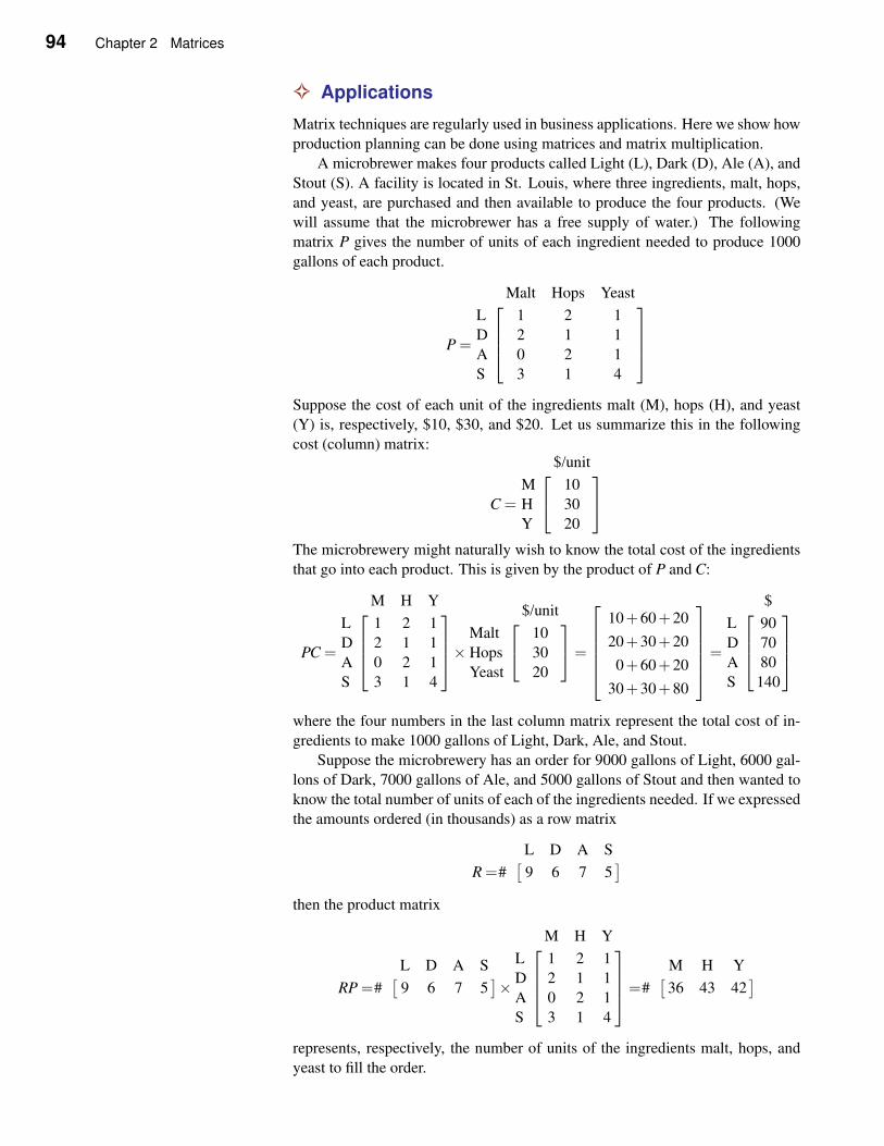
94 Chapter 2 Matrices
✧ Applications
Matrix techniques are regularly used in business applications. Here we show how
production planning can be done using matrices and matrix multiplication.
A microbrewer makes four products called Light (L), Dark (D), Ale (A), and
Stout (S). A facility is located in St. Louis, where three ingredients, malt, hops,
and yeast, are purchased and then available to produce the four products. (We
will assume that the microbrewer has a free supply of water.) The following
matrix P gives the number of units of each ingredient needed to produce 1000
gallons of each product.
P =
Malt Hops Yeast
L 1 2 1
D 2 1 1
A 0 2 1
S 3 1 4
Suppose the cost of each unit of the ingredients malt (M), hops (H), and yeast
(Y) is, respectively, $10, $30, and $20. Let us summarize this in the following
cost (column) matrix:
C =
$/unit
M 10
H 30
Y 20
The microbrewery might naturally wish to know the total cost of the ingredients
that go into each product. This is given by the product of P and C:
PC =
M H Y
L 1 2 1
D 2 1 1
A 0 2 1
S 3 1 4
×
$/unit
Malt 10
Hops 30
Yeast 20
=
10+60+20
20+30+20
0+60+20
30+30+80
=
$
L 90
D 70
A 80
S 140
where the four numbers in the last column matrix represent the total cost of in-
gredients to make 1000 gallons of Light, Dark, Ale, and Stout.
Suppose the microbrewery has an order for 9000 gallons of Light, 6000 gal-
lons of Dark, 7000 gallons of Ale, and 5000 gallons of Stout and then wanted to
know the total number of units of each of the ingredients needed. If we expressed
the amounts ordered (in thousands) as a row matrix
R =[
L D A S
# 9 6 7 5]
then the product matrix
RP =[
L D A S
# 9 6 7 5]×
M H Y
L 1 2 1
D 2 1 1
A 0 2 1
S 3 1 4
=
[M H Y
# 36 43 42]
represents, respectively, the number of units of the ingredients malt, hops, and
yeast to fill the order.
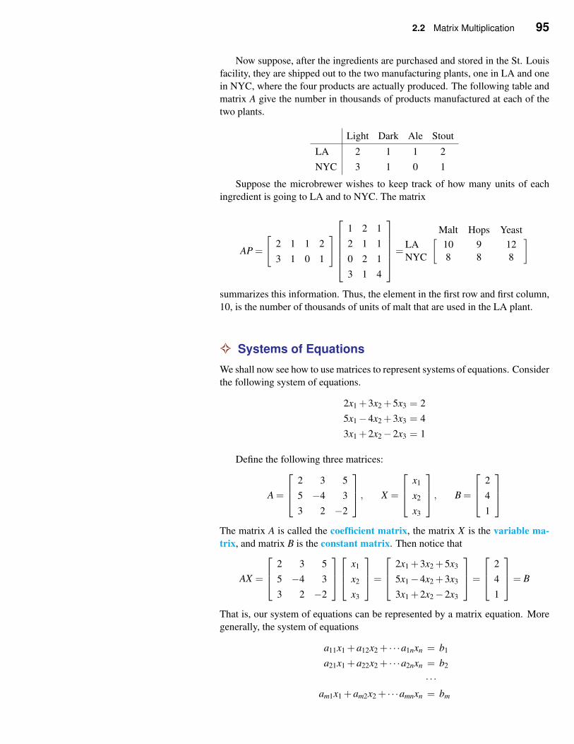
2.2 Matrix Multiplication 95
Now suppose, after the ingredients are purchased and stored in the St. Louis
facility, they are shipped out to the two manufacturing plants, one in LA and one
in NYC, where the four products are actually produced. The following table and
matrix A give the number in thousands of products manufactured at each of the
two plants.
Light Dark Ale Stout
LA 2 1 1 2
NYC 3 1 0 1
Suppose the microbrewer wishes to keep track of how many units of each
ingredient is going to LA and to NYC. The matrix
AP =
[
2 1 1 2
3 1 0 1
]
1 2 1
2 1 1
0 2 1
3 1 4
=
[Malt Hops Yeast
LA 10 9 12
NYC 8 8 8
]
summarizes this information. Thus, the element in the first row and first column,
10, is the number of thousands of units of malt that are used in the LA plant.
✧ Systems of Equations
We shall now see how to use matrices to represent systems of equations. Consider
the following system of equations.
2x1 +3x2 +5x3 = 2
5x1−4x2 +3x3 = 4
3x1 +2x2−2x3 = 1
Define the following three matrices:
A =
2 3 5
5 −4 3
3 2 −2
, X =
x1
x2
x3
, B =
2
4
1
The matrix A is called the coefficient matrix, the matrix X is the variable ma-
trix, and matrix B is the constant matrix. Then notice that
AX =
2 3 5
5 −4 3
3 2 −2
x1
x2
x3
=
2x1 +3x2 +5x3
5x1−4x2 +3x3
3x1 +2x2−2x3
=
2
4
1
= B
That is, our system of equations can be represented by a matrix equation. More
generally, the system of equations
a11x1 +a12x2 + · · ·a1nxn = b1
a21x1 +a22x2 + · · ·a2nxn = b2
· · ·am1x1 +am2x2 + · · ·amnxn = bm
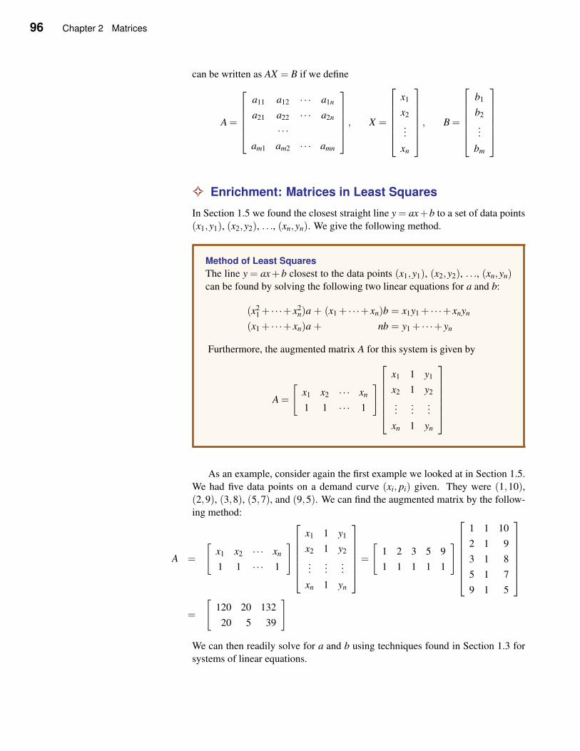
96 Chapter 2 Matrices
can be written as AX = B if we define
A =
a11 a12 · · · a1n
a21 a22 · · · a2n
· · ·am1 am2 · · · amn
, X =
x1
x2
...
xn
, B =
b1
b2
...
bm
✧ Enrichment: Matrices in Least Squares
In Section 1.5 we found the closest straight line y = ax+b to a set of data points
(x1,y1), (x2,y2), . . ., (xn,yn). We give the following method.
Method of Least Squares
The line y = ax+ b closest to the data points (x1,y1), (x2,y2), . . ., (xn,yn)can be found by solving the following two linear equations for a and b:
(x21 + · · ·+ x2
n)a + (x1 + · · ·+ xn)b = x1y1 + · · ·+ xnyn
(x1 + · · ·+ xn)a + nb = y1 + · · ·+ yn
Furthermore, the augmented matrix A for this system is given by
A =
[
x1 x2 · · · xn
1 1 · · · 1
]
x1 1 y1
x2 1 y2
......
...
xn 1 yn
As an example, consider again the first example we looked at in Section 1.5.
We had five data points on a demand curve (xi, pi) given. They were (1,10),(2,9), (3,8), (5,7), and (9,5). We can find the augmented matrix by the follow-
ing method:
A =
[
x1 x2 · · · xn
1 1 · · · 1
]
x1 1 y1
x2 1 y2
......
...
xn 1 yn
=
[
1 2 3 5 9
1 1 1 1 1
]
1 1 10
2 1 9
3 1 8
5 1 7
9 1 5
=
[
120 20 132
20 5 39
]
We can then readily solve for a and b using techniques found in Section 1.3 for
systems of linear equations.
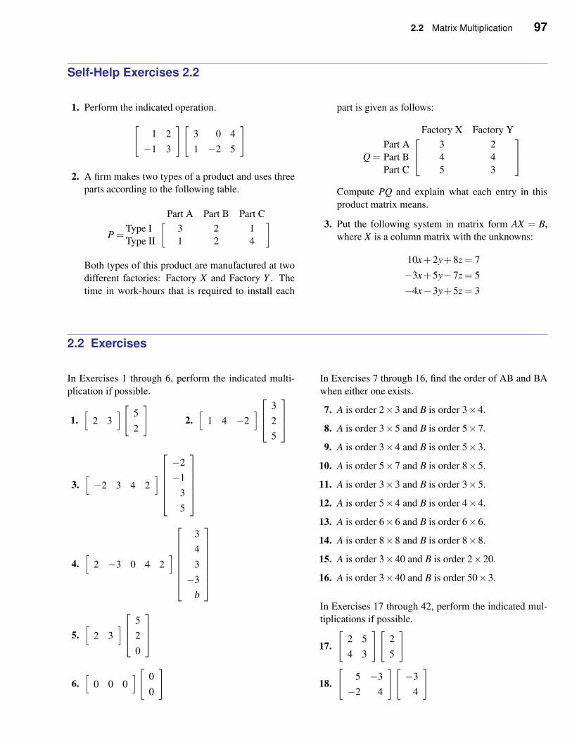
2.2 Matrix Multiplication 97
Self-Help Exercises 2.2
1. Perform the indicated operation.
[
1 2
−1 3
][
3 0 4
1 −2 5
]
2. A firm makes two types of a product and uses three
parts according to the following table.
P =
[Part A Part B Part C
Type I 3 2 1
Type II 1 2 4
]
Both types of this product are manufactured at two
different factories: Factory X and Factory Y . The
time in work-hours that is required to install each
part is given as follows:
Q =
Factory X Factory Y
Part A 3 2
Part B 4 4
Part C 5 3
Compute PQ and explain what each entry in this
product matrix means.
3. Put the following system in matrix form AX = B,
where X is a column matrix with the unknowns:
10x+2y+8z = 7
−3x+5y−7z = 5
−4x−3y+5z = 3
2.2 Exercises
In Exercises 1 through 6, perform the indicated multi-
plication if possible.
1.[
2 3][
5
2
]
2.[
1 4 −2]
3
2
5
3.[
−2 3 4 2]
−2
−1
3
5
4.[
2 −3 0 4 2]
3
4
3
−3
b
5.[
2 3]
5
2
0
6.[
0 0 0][
0
0
]
In Exercises 7 through 16, find the order of AB and BA
when either one exists.
7. A is order 2×3 and B is order 3×4.
8. A is order 3×5 and B is order 5×7.
9. A is order 3×4 and B is order 5×3.
10. A is order 5×7 and B is order 8×5.
11. A is order 3×3 and B is order 3×5.
12. A is order 5×4 and B is order 4×4.
13. A is order 6×6 and B is order 6×6.
14. A is order 8×8 and B is order 8×8.
15. A is order 3×40 and B is order 2×20.
16. A is order 3×40 and B is order 50×3.
In Exercises 17 through 42, perform the indicated mul-
tiplications if possible.
17.
[
2 5
4 3
][
2
5
]
18.
[
5 −3
−2 4
][
−3
4
]
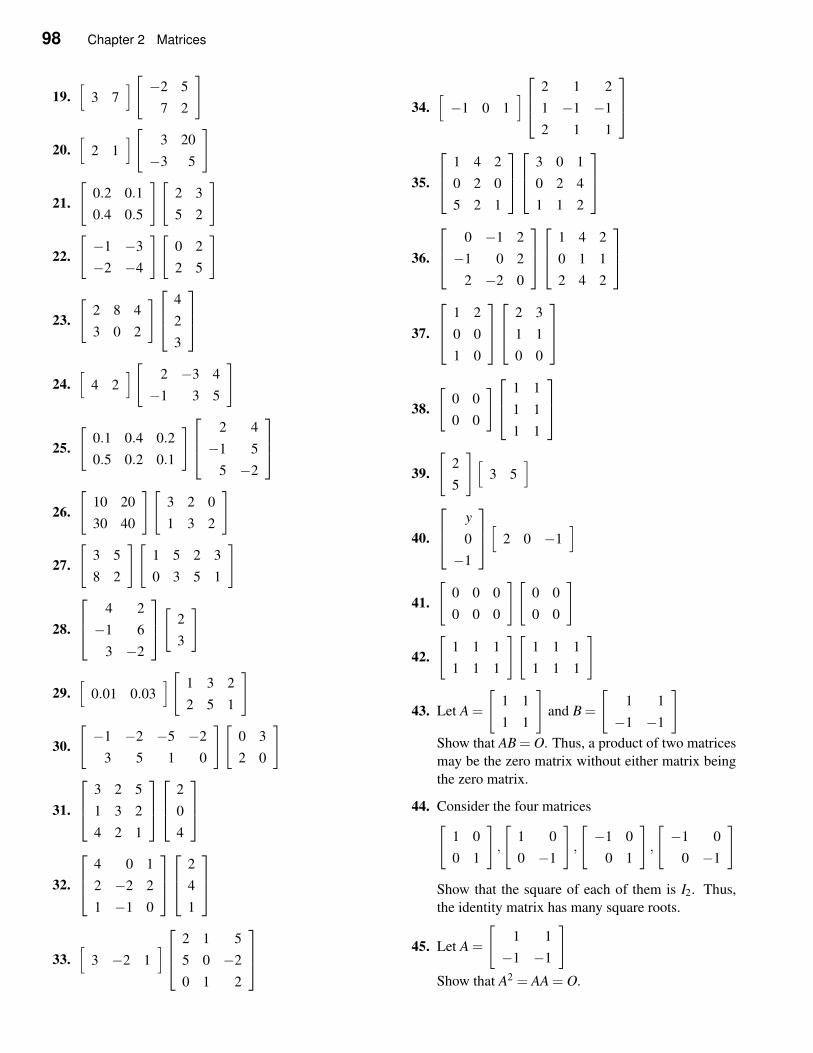
98 Chapter 2 Matrices
19.[
3 7][
−2 5
7 2
]
20.[
2 1][
3 20
−3 5
]
21.
[
0.2 0.1
0.4 0.5
][
2 3
5 2
]
22.
[
−1 −3
−2 −4
][
0 2
2 5
]
23.
[
2 8 4
3 0 2
]
4
2
3
24.[
4 2][
2 −3 4
−1 3 5
]
25.
[
0.1 0.4 0.2
0.5 0.2 0.1
]
2 4
−1 5
5 −2
26.
[
10 20
30 40
][
3 2 0
1 3 2
]
27.
[
3 5
8 2
][
1 5 2 3
0 3 5 1
]
28.
4 2
−1 6
3 −2
[
2
3
]
29.[
0.01 0.03][
1 3 2
2 5 1
]
30.
[
−1 −2 −5 −2
3 5 1 0
][
0 3
2 0
]
31.
3 2 5
1 3 2
4 2 1
2
0
4
32.
4 0 1
2 −2 2
1 −1 0
2
4
1
33.[
3 −2 1]
2 1 5
5 0 −2
0 1 2
34.[
−1 0 1]
2 1 2
1 −1 −1
2 1 1
35.
1 4 2
0 2 0
5 2 1
3 0 1
0 2 4
1 1 2
36.
0 −1 2
−1 0 2
2 −2 0
1 4 2
0 1 1
2 4 2
37.
1 2
0 0
1 0
2 3
1 1
0 0
38.
[
0 0
0 0
]
1 1
1 1
1 1
39.
[
2
5
][
3 5]
40.
y
0
−1
[
2 0 −1]
41.
[
0 0 0
0 0 0
][
0 0
0 0
]
42.
[
1 1 1
1 1 1
][
1 1 1
1 1 1
]
43. Let A =
[
1 1
1 1
]
and B =
[
1 1
−1 −1
]
Show that AB = O. Thus, a product of two matrices
may be the zero matrix without either matrix being
the zero matrix.
44. Consider the four matrices[
1 0
0 1
]
,
[
1 0
0 −1
]
,
[
−1 0
0 1
]
,
[
−1 0
0 −1
]
Show that the square of each of them is I2. Thus,
the identity matrix has many square roots.
45. Let A =
[
1 1
−1 −1
]
Show that A2 = AA = O.
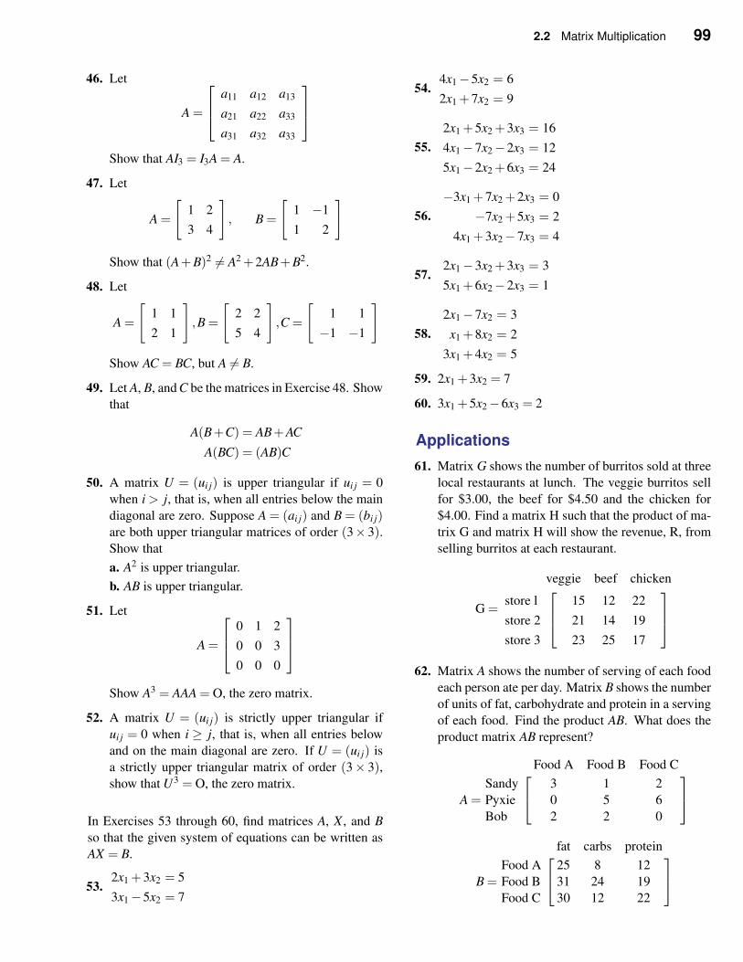
2.2 Matrix Multiplication 99
46. Let
A =
a11 a12 a13
a21 a22 a33
a31 a32 a33
Show that AI3 = I3A = A.
47. Let
A =
[
1 2
3 4
]
, B =
[
1 −1
1 2
]
Show that (A+B)2 6= A2 +2AB+B2.
48. Let
A =
[
1 1
2 1
]
,B =
[
2 2
5 4
]
,C =
[
1 1
−1 −1
]
Show AC = BC, but A 6= B.
49. Let A, B, and C be the matrices in Exercise 48. Show
that
A(B+C) = AB+AC
A(BC) = (AB)C
50. A matrix U = (ui j) is upper triangular if ui j = 0
when i > j, that is, when all entries below the main
diagonal are zero. Suppose A = (ai j) and B = (bi j)are both upper triangular matrices of order (3× 3).Show that
a. A2 is upper triangular.
b. AB is upper triangular.
51. Let
A =
0 1 2
0 0 3
0 0 0
Show A3 = AAA = O, the zero matrix.
52. A matrix U = (ui j) is strictly upper triangular if
ui j = 0 when i ≥ j, that is, when all entries below
and on the main diagonal are zero. If U = (ui j) is
a strictly upper triangular matrix of order (3× 3),show that U3 = O, the zero matrix.
In Exercises 53 through 60, find matrices A, X , and B
so that the given system of equations can be written as
AX = B.
53.2x1 +3x2 = 5
3x1−5x2 = 7
54.4x1−5x2 = 6
2x1 +7x2 = 9
55.
2x1 +5x2 +3x3 = 16
4x1−7x2−2x3 = 12
5x1−2x2 +6x3 = 24
56.
−3x1 +7x2 +2x3 = 0
−7x2 +5x3 = 2
4x1 +3x2−7x3 = 4
57.2x1−3x2 +3x3 = 3
5x1 +6x2−2x3 = 1
58.
2x1−7x2 = 3
x1 +8x2 = 2
3x1 +4x2 = 5
59. 2x1 +3x2 = 7
60. 3x1 +5x2−6x3 = 2
Applications
61. Matrix G shows the number of burritos sold at three
local restaurants at lunch. The veggie burritos sell
for $3.00, the beef for $4.50 and the chicken for
$4.00. Find a matrix H such that the product of ma-
trix G and matrix H will show the revenue, R, from
selling burritos at each restaurant.
G =
veggie beef chicken
store l
store 2
store 3
15 12 22
21 14 19
23 25 17
62. Matrix A shows the number of serving of each food
each person ate per day. Matrix B shows the number
of units of fat, carbohydrate and protein in a serving
of each food. Find the product AB. What does the
product matrix AB represent?
A =
Food A Food B Food C
Sandy 3 1 2
Pyxie 0 5 6
Bob 2 2 0
B =
fat carbs protein
Food A 25 8 12
Food B 31 24 19
Food C 30 12 22
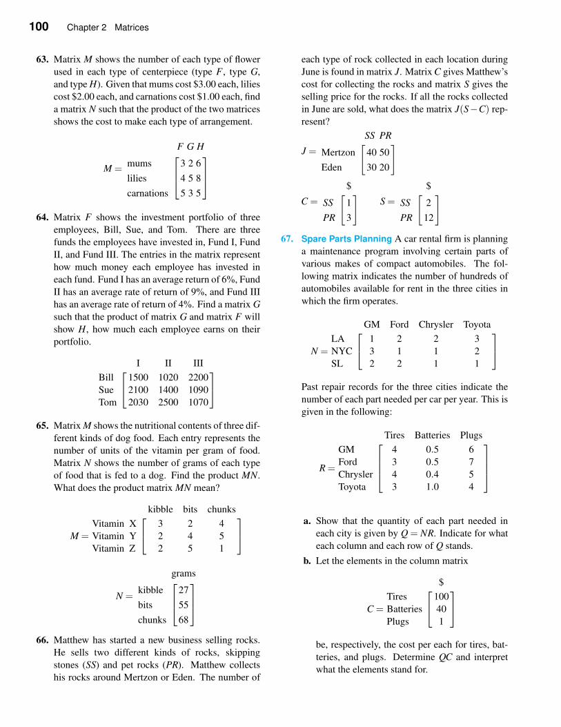
100 Chapter 2 Matrices
63. Matrix M shows the number of each type of flower
used in each type of centerpiece (type F , type G,
and type H). Given that mums cost $3.00 each, lilies
cost $2.00 each, and carnations cost $1.00 each, find
a matrix N such that the product of the two matrices
shows the cost to make each type of arrangement.
M =
F G H
mums
lilies
carnations
3 2 6
4 5 8
5 3 5
64. Matrix F shows the investment portfolio of three
employees, Bill, Sue, and Tom. There are three
funds the employees have invested in, Fund I, Fund
II, and Fund III. The entries in the matrix represent
how much money each employee has invested in
each fund. Fund I has an average return of 6%, Fund
II has an average rate of return of 9%, and Fund III
has an average rate of return of 4%. Find a matrix G
such that the product of matrix G and matrix F will
show H, how much each employee earns on their
portfolio.
I II III
Bill 1500 1020 2200
Sue 2100 1400 1090
Tom 2030 2500 1070
65. Matrix M shows the nutritional contents of three dif-
ferent kinds of dog food. Each entry represents the
number of units of the vitamin per gram of food.
Matrix N shows the number of grams of each type
of food that is fed to a dog. Find the product MN.
What does the product matrix MN mean?
M =
kibble bits chunks
Vitamin X 3 2 4
Vitamin Y 2 4 5
Vitamin Z 2 5 1
N =
grams
kibble
bits
chunks
27
55
68
66. Matthew has started a new business selling rocks.
He sells two different kinds of rocks, skipping
stones (SS) and pet rocks (PR). Matthew collects
his rocks around Mertzon or Eden. The number of
each type of rock collected in each location during
June is found in matrix J. Matrix C gives Matthew’s
cost for collecting the rocks and matrix S gives the
selling price for the rocks. If all the rocks collected
in June are sold, what does the matrix J(S−C) rep-
resent?
J =
SS PR
Mertzon
Eden
[
40 50
30 20
]
C =
$
SS
PR
[
1
3
]
S =
$
SS
PR
[
2
12
]
67. Spare Parts Planning A car rental firm is planning
a maintenance program involving certain parts of
various makes of compact automobiles. The fol-
lowing matrix indicates the number of hundreds of
automobiles available for rent in the three cities in
which the firm operates.
N =
GM Ford Chrysler Toyota
LA 1 2 2 3
NYC 3 1 1 2
SL 2 2 1 1
Past repair records for the three cities indicate the
number of each part needed per car per year. This is
given in the following:
R =
Tires Batteries Plugs
GM 4 0.5 6
Ford 3 0.5 7
Chrysler 4 0.4 5
Toyota 3 1.0 4
a. Show that the quantity of each part needed in
each city is given by Q = NR. Indicate for what
each column and each row of Q stands.
b. Let the elements in the column matrix
C =
$
Tires 100
Batteries 40
Plugs 1
be, respectively, the cost per each for tires, bat-
teries, and plugs. Determine QC and interpret
what the elements stand for.
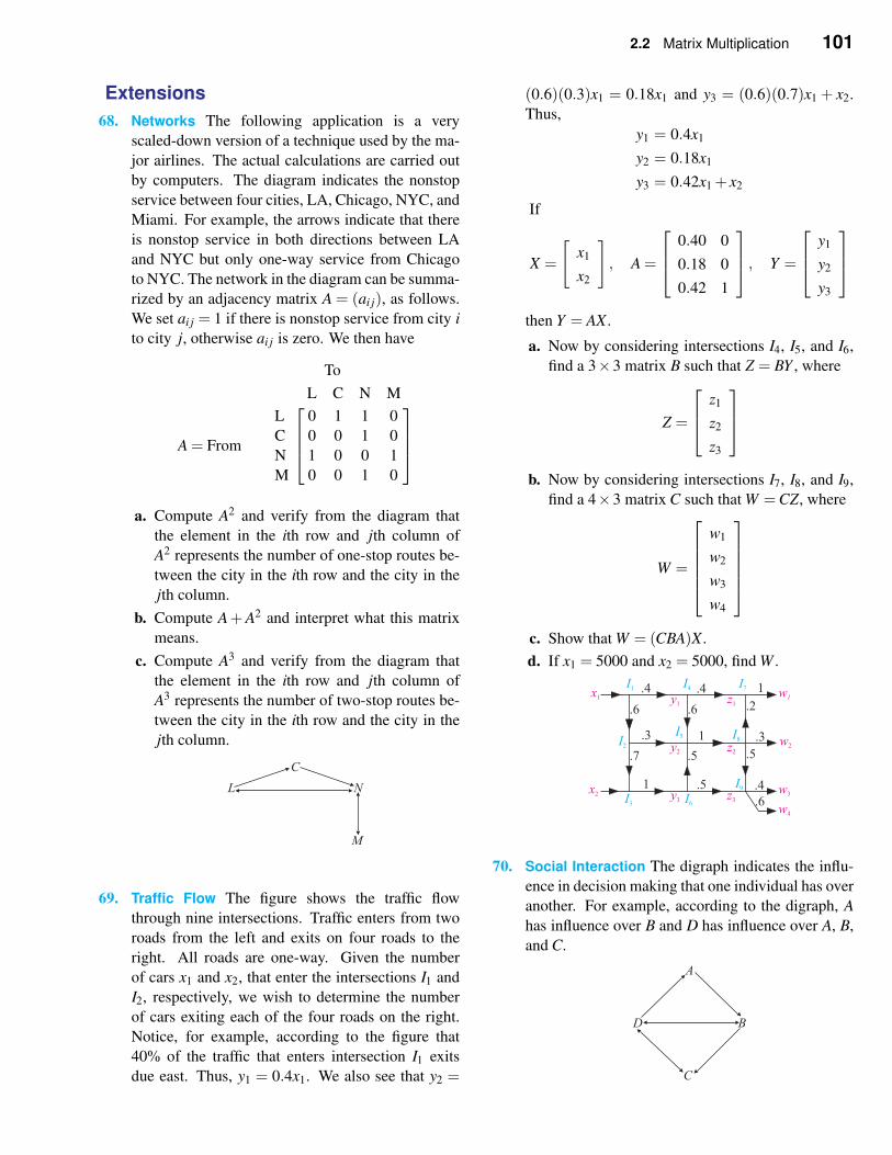
2.2 Matrix Multiplication 101
Extensions
68. Networks The following application is a very
scaled-down version of a technique used by the ma-
jor airlines. The actual calculations are carried out
by computers. The diagram indicates the nonstop
service between four cities, LA, Chicago, NYC, and
Miami. For example, the arrows indicate that there
is nonstop service in both directions between LA
and NYC but only one-way service from Chicago
to NYC. The network in the diagram can be summa-
rized by an adjacency matrix A = (ai j), as follows.
We set ai j = 1 if there is nonstop service from city i
to city j, otherwise ai j is zero. We then have
To
A = From
L C N M
L 0 1 1 0
C 0 0 1 0
N 1 0 0 1
M 0 0 1 0
a. Compute A2 and verify from the diagram that
the element in the ith row and jth column of
A2 represents the number of one-stop routes be-
tween the city in the ith row and the city in the
jth column.
b. Compute A+A2 and interpret what this matrix
means.
c. Compute A3 and verify from the diagram that
the element in the ith row and jth column of
A3 represents the number of two-stop routes be-
tween the city in the ith row and the city in the
jth column.
69. Traffic Flow The figure shows the traffic flow
through nine intersections. Traffic enters from two
roads from the left and exits on four roads to the
right. All roads are one-way. Given the number
of cars x1 and x2, that enter the intersections I1 and
I2, respectively, we wish to determine the number
of cars exiting each of the four roads on the right.
Notice, for example, according to the figure that
40% of the traffic that enters intersection I1 exits
due east. Thus, y1 = 0.4x1. We also see that y2 =
(0.6)(0.3)x1 = 0.18x1 and y3 = (0.6)(0.7)x1 + x2.
Thus,
y1 = 0.4x1
y2 = 0.18x1
y3 = 0.42x1 + x2
If
X =
[
x1
x2
]
, A =
0.40 0
0.18 0
0.42 1
, Y =
y1
y2
y3
then Y = AX .
a. Now by considering intersections I4, I5, and I6,
find a 3×3 matrix B such that Z = BY , where
Z =
z1
z2
z3
b. Now by considering intersections I7, I8, and I9,
find a 4×3 matrix C such that W =CZ, where
W =
w1
w2
w3
w4
c. Show that W = (CBA)X .
d. If x1 = 5000 and x2 = 5000, find W .
70. Social Interaction The digraph indicates the influ-
ence in decision making that one individual has over
another. For example, according to the digraph, A
has influence over B and D has influence over A, B,
and C.
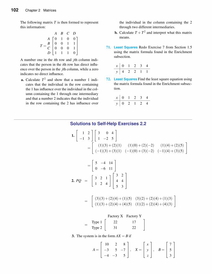
102 Chapter 2 Matrices
The following matrix T is then formed to represent
this information:
T =
A B C D
A 0 1 0 0
B 0 0 1 1
C 0 0 0 1
D 1 1 1 0
A number one in the ith row and jth column indi-
cates that the person in the ith row has direct influ-
ence over the person in the jth column, while a zero
indicates no direct influence.
a. Calculate T 2 and show that a number 1 indi-
cates that the individual in the row containing
the 1 has influence over the individual in the col-
umn containing the 1 through one intermediary
and that a number 2 indicates that the individual
in the row containing the 2 has influence over
the individual in the column containing the 2
through two different intermediaries.
b. Calculate T +T 2 and interpret what this matrix
means.
71. Least Squares Redo Exercise 7 from Section 1.5
using the matrix formula found in the Enrichment
subsection.
x 0 1 2 3 4
y 4 2 2 1 1
72. Least Squares Find the least square equation using
the matrix formula found in the Enrichment subsec-
tion.
x 0 1 2 3 4
y 0 2 1 2 4
Solutions to Self-Help Exercises 2.2
1.
[
1 2
−1 3
][
3 0 4
1 −2 5
]
=
[
(1)(3)+(2)(1) (1)(0)+(2)(−2) (1)(4)+(2)(5)
(−1)(3)+(3)(1) (−1)(0)+(3)(−2) (−1)(4)+(3)(5)
]
=
[
5 −4 14
0 −6 11
]
2. PQ =
[
3 2 1
1 2 4
]
3 2
4 4
5 3
=
[
(3)(3)+(2)(4)+(1)(5) (3)(2)+(2)(4)+(1)(3)
(1)(3)+(2)(4)+(4)(5) (1)(2)+(2)(4)+(4)(3)
]
=
[Factory X Factory Y
Type 1 22 17
Type 2 31 22
]
3. The system is in the form AX = B if
A =
10 2 8
−3 5 −7
−4 −3 5
, X =
x
y
z
, B =
7
5
3
2.3 Inverse of a Square Matrix 103
2.3 Inverse of a Square Matrix
APPLICATION
Allocation of Funds
An investment adviser has two mutual funds that she is recommending: a
conservative bond fund with an assumed return of 7% a year and a stock
fund with a projected return of 12% a year. One client has $100,000 to
invest and wishes a return of 9% a year, and a second client has $50,000
and wants a 10% annual return. How should she allocate the money of each
client between the bond fund and the stock fund? The answer is found in
Example 4.
✧ Definition of the Inverse of a Matrix
In this section we will define the inverse of a square matrix and will see that
the inverse matrix is an extremely powerful tool in solving systems of equations
where the number of unknowns is the same as the number of equations. We will
develop a technique to find the inverse of a square matrix. We will also explore
other applications of matrix inverses such as decoding messages (cryptography).
The equation ax = 1 has the solution x = 1/a = a−1 if a 6= 0. The number
a−1 is the reciprocal, or inverse, of the real number a and it has the property that
aa−1 = a−1a = 1. All real numbers except 0 have an inverse. We wish to find the
matrix equivalent of this relationship. That is, given a square n×n matrix A, we
wish to find a matrix A−1 called the inverse of A with the property that
AA−1 = A−1A = In
where In is the n×n identity matrix.
Inverse Matrix
The n×n matrix B is said to be the inverse to the n×n matrix A if
AB = BA = In
If the inverse matrix B exists, we write B = A−1.
REMARK: Do not think that the inverse matrix A−1 can be written as 1/A. We
never divide matrices.
HISTORICAL NOTE
Arthur Cayley
1821–1895
Arthur Cayley was the first to
consider the idea of an inverse to a
matrix in 1855. Cayley was
educated in England and, unable
to find a suitable teaching position,
studied and practiced law for 14
years. During this time he
published about 300 papers in
mathematics. Eventually he
become a professor at Cambridge
in 1863. Cayley was acquainted
with James Sylvester, mentioned in
an earlier section, and together
their collaborations resulted in
many outstanding results in
mathematics. Cayley was an
enormously prolific researcher; his
collected works contain 966 papers
in thirteen volumes, each volume
containing about 600 pages.
EXAMPLE 1 Showing a Matrix Is the Inverse Matrix Let
A =
[
3 1
5 2
]
Then show that the inverse of A is
A−1 =
[
2 −1
−5 3
]
104 Chapter 2 Matrices
Solution Find AA−1 and A−1A,
AA−1 =
[
3 1
5 2
][
2 −1
−5 3
]
=
[
1 0
0 1
]
= I2
and
A−1A =
[
2 −1
−5 3
][
3 1
5 2
]
=
[
1 0
0 1
]
= I2
Since AA−1 = I = A−1A, A−1 is the inverse of A. ✦
Not every matrix has an inverse. Consider B =
[
2 1
4 2
]
. Let us try to find a
2×2 matrix X such that BX = I2,
[
1 0
0 1
]
= I2 = BX =
[
2 1
4 2
][
a b
c d
]
=
[
2a+ c 2b+d
4a+2c 4b+2d
]
Using the property of matrix equality gives the following two of the four equa-
tions.2a+ c = 1
4a+2c = 0
But 2 times the first of these two equations yields 4a+2c= 2. This is inconsistent
with the second equation, and thus no solution can exist. This shows that B−1
does not exist. If the inverse does not exist, the matrix is called singular.
✧ Finding the Inverse
We shall now develop a technique that will find the inverse of a square matrix, if
it exists, or indicate that the inverse does not exist. Consider
A =
[
1 2
3 7
]
To find
A−1 = X =
[
x1 y1
x2 y2
]
we must solve the equation AX = I2 or
AX =
[
1 2
3 7
][
x1 y1
x2 y2
]
=
[
x1 +2x2 y1 +2y2
3x1 +7x2 3y1 +7y2
]
=
[
1 0
0 1
]
This gives the four equations
x1 +2x2 = 1 y1 +2y2 = 0
3x1 +7x2 = 0 3y1 +7y2 = 1
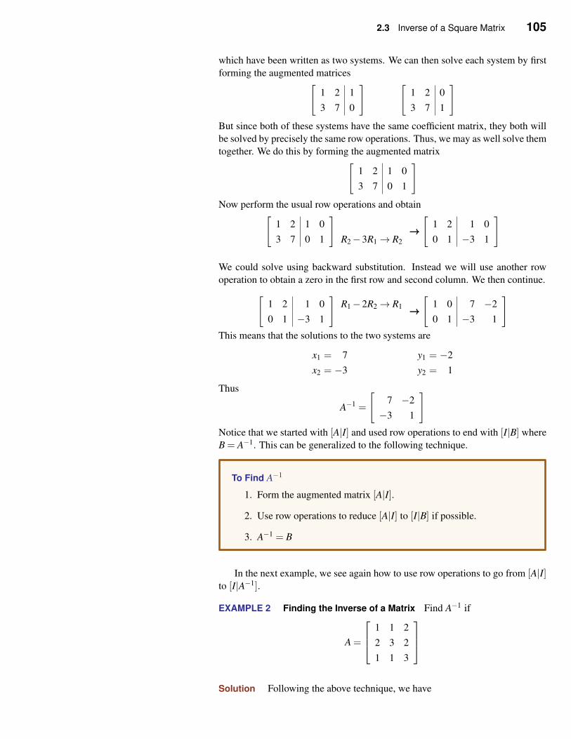
2.3 Inverse of a Square Matrix 105
which have been written as two systems. We can then solve each system by first
forming the augmented matrices[
1 2 1
3 7 0
] [
1 2 0
3 7 1
]
But since both of these systems have the same coefficient matrix, they both will
be solved by precisely the same row operations. Thus, we may as well solve them
together. We do this by forming the augmented matrix[
1 2 1 0
3 7 0 1
]
Now perform the usual row operations and obtain[
1 2 1 0
3 7 0 1
]
R2−3R1→ R2
→→→[
1 2 1 0
0 1 −3 1
]
We could solve using backward substitution. Instead we will use another row
operation to obtain a zero in the first row and second column. We then continue.
[
1 2 1 0
0 1 −3 1
]
R1−2R2→ R1 →→→[
1 0 7 −2
0 1 −3 1
]
This means that the solutions to the two systems are
x1 = 7
x2 = −3
y1 = −2
y2 = 1
Thus
A−1 =
[
7 −2
−3 1
]
Notice that we started with [A|I] and used row operations to end with [I|B] where
B = A−1. This can be generalized to the following technique.
To Find A−1
1. Form the augmented matrix [A|I].
2. Use row operations to reduce [A|I] to [I|B] if possible.
3. A−1 = B
In the next example, we see again how to use row operations to go from [A|I]to [I|A−1].
EXAMPLE 2 Finding the Inverse of a Matrix Find A−1 if
A =
1 1 2
2 3 2
1 1 3
Solution Following the above technique, we have
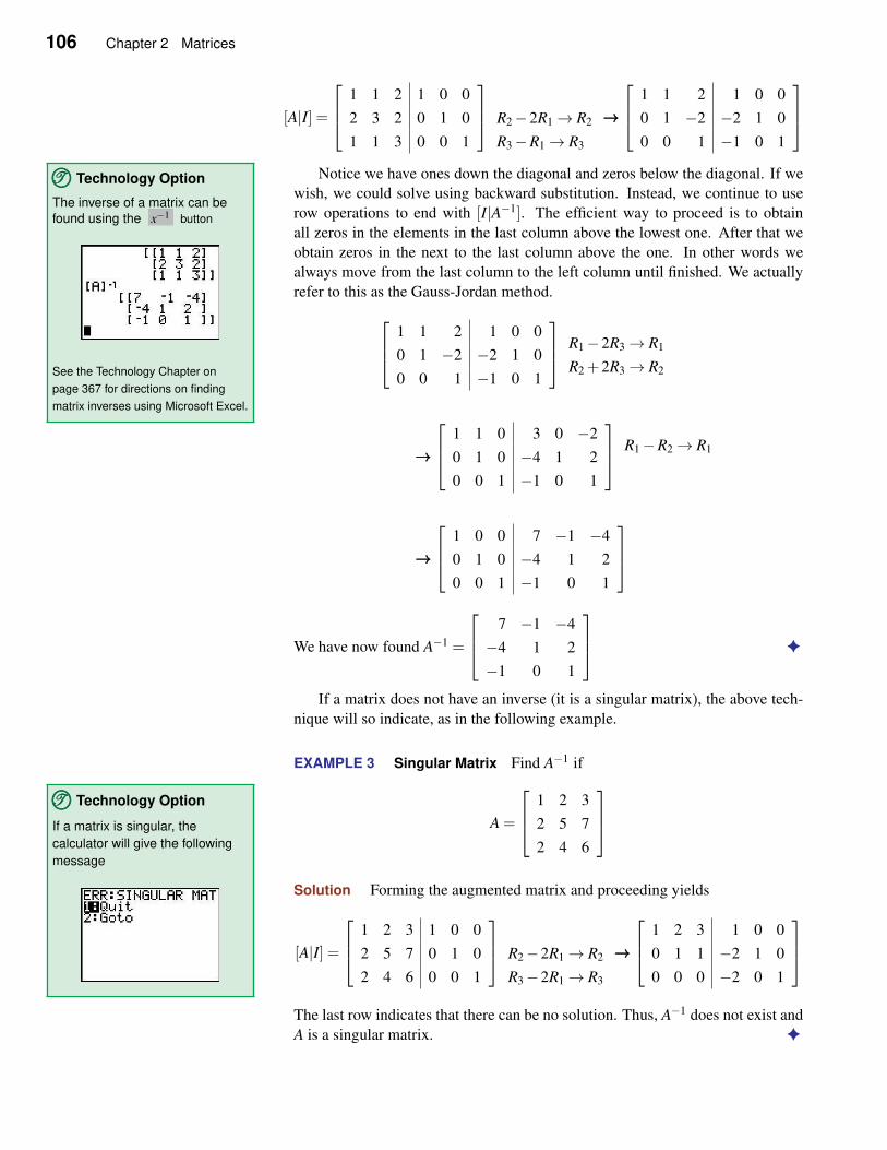
106 Chapter 2 Matrices
[A|I] =
1 1 2 1 0 0
2 3 2 0 1 0
1 1 3 0 0 1
R2−2R1→ R2
R3−R1→ R3
→→→
1 1 2 1 0 0
0 1 −2 −2 1 0
0 0 1 −1 0 1
Notice we have ones down the diagonal and zeros below the diagonal. If we
wish, we could solve using backward substitution. Instead, we continue to use
row operations to end with [I|A−1]. The efficient way to proceed is to obtain
all zeros in the elements in the last column above the lowest one. After that we
obtain zeros in the next to the last column above the one. In other words we
always move from the last column to the left column until finished. We actually
refer to this as the Gauss-Jordan method.
TTT©©© Technology Option
The inverse of a matrix can befound using the x−1 button
See the Technology Chapter on
page 367 for directions on finding
matrix inverses using Microsoft Excel.
1 1 2 1 0 0
0 1 −2 −2 1 0
0 0 1 −1 0 1
R1−2R3→ R1
R2 +2R3→ R2
→→→
1 1 0 3 0 −2
0 1 0 −4 1 2
0 0 1 −1 0 1
R1−R2→ R1
→→→
1 0 0 7 −1 −4
0 1 0 −4 1 2
0 0 1 −1 0 1
We have now found A−1 =
7 −1 −4
−4 1 2
−1 0 1
✦
If a matrix does not have an inverse (it is a singular matrix), the above tech-
nique will so indicate, as in the following example.
EXAMPLE 3 Singular Matrix Find A−1 if
A =
1 2 3
2 5 7
2 4 6
Solution Forming the augmented matrix and proceeding yields
TTT©©© Technology Option
If a matrix is singular, the
calculator will give the following
message
[A|I] =
1 2 3 1 0 0
2 5 7 0 1 0
2 4 6 0 0 1
R2−2R1→ R2
R3−2R1→ R3
→→→
1 2 3 1 0 0
0 1 1 −2 1 0
0 0 0 −2 0 1
The last row indicates that there can be no solution. Thus, A−1 does not exist and
A is a singular matrix. ✦
2.3 Inverse of a Square Matrix 107
✧ Systems of Equations
We shall now see how the inverse matrix can be used to solve systems of equa-
tions with the number of unknowns equal to the number of equations. Consider
the system
a11x1 +a12x2 + · · ·a1nxn = b1
a21x1 +a22x2 + · · ·a2nxn = b2
· · ·an1x1 +an2x2 + · · ·annxn = bn
If A =
a11 a12 · · · a1n
a21 a22 · · · a2n
· · ·an1 an2 · · · ann
, X =
x1
x2
...
xn
, B =
b1
b2
...
bn
then the system can be written as
AX = B
If this was the numerical equation ax = b with a 6= 0, you would divide both
sides by a to obtain the solution for x as x = b/a. However, this is a matrix
equation, so we must multiply by the inverse, rather than dividing. Now if A−1
exists (that is, A is nonsingular), multiply both sides of AX = B on the left by
A−1, obtaining
A−1(AX) = A−1B
Note that we left-multiplied both sides by A−1. The fact that matrix multiplication
is non-commutative means that not only do you need to do the same operation
on both sides of the matrix equation as in regular algebra, but you must also take
care to do it on the same side. Now the left side is
A−1(AX) = (A−1A)X = InX = X
Thus, X = A−1B is the solution of the system.
Solution of AX = B
Let A be a square matrix of order n and B a column matrix of order n. If
A−1 exists, then the linear system of equations
AX = B
has the unique solution
X = A−1B
REMARK: If A−1 does not exist, then the system of equations does not have
a single, unique solution. The system must have a parametric solution or no
solution in this case.
EXAMPLE 4 Solving Systems of Equations Using Matrices Solve the
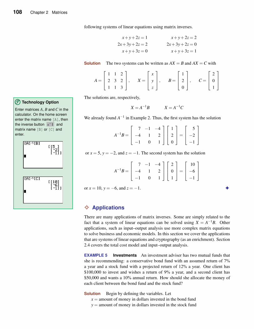
108 Chapter 2 Matrices
following systems of linear equations using matrix inverses.
x+ y+2z = 1 x+ y+2z = 2
2x+3y+2z = 2 2x+3y+2z = 0
x+ y+3z = 0 x+ y+3z = 1
Solution The two systems can be written as AX = B and AX =C with
A =
1 1 2
2 3 2
1 1 3
, X =
x
y
z
, B =
1
2
0
, C =
2
0
1
The solutions are, respectively,
X = A−1B X = A−1C
We already found A−1 in Example 2. Thus, the first system has the solution
A−1B =
7 −1 −4
−4 1 2
−1 0 1
1
2
0
=
5
−2
−1
or x = 5, y =−2, and z =−1. The second system has the solution
TTT©©© Technology Option
Enter matrices A, B and C in the
calculator. On the home screen
enter the matrix name [A], then
the inverse button x−1 and
matrix name [B] or [C] and
enter.
A−1B =
7 −1 −4
−4 1 2
−1 0 1
2
0
1
=
10
−6
−1
or x = 10, y =−6, and z =−1. ✦
✧ Applications
There are many applications of matrix inverses. Some are simply related to the
fact that a system of linear equations can be solved using X = A−1B. Other
applications, such as input–output analysis use more complex matrix equations
to solve business and economic models. In this section we cover the applications
that are systems of linear equations and cryptography (as an enrichment). Section
2.4 covers the total cost model and input–output analysis.
EXAMPLE 5 Investments An investment adviser has two mutual funds that
she is recommending: a conservative bond fund with an assumed return of 7%
a year and a stock fund with a projected return of 12% a year. One client has
$100,000 to invest and wishes a return of 9% a year, and a second client has
$50,000 and wants a 10% annual return. How should she allocate the money of
each client between the bond fund and the stock fund?
Solution Begin by defining the variables. Let
x = amount of money in dollars invested in the bond fund
y = amount of money in dollars invested in the stock fund
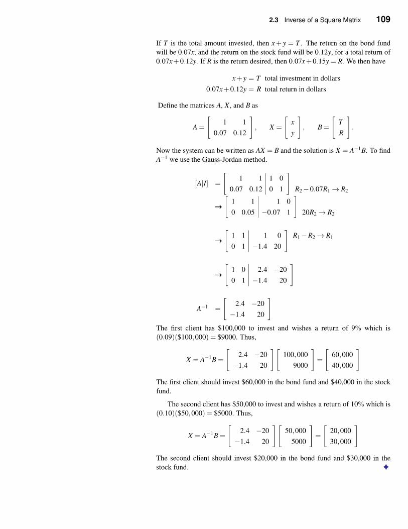
2.3 Inverse of a Square Matrix 109
If T is the total amount invested, then x+ y = T . The return on the bond fund
will be 0.07x, and the return on the stock fund will be 0.12y, for a total return of
0.07x+0.12y. If R is the return desired, then 0.07x+0.15y = R. We then have
x+ y = T total investment in dollars
0.07x+0.12y = R total return in dollars
Define the matrices A, X , and B as
A =
[
1 1
0.07 0.12
]
, X =
[
x
y
]
, B =
[
T
R
]
.
Now the system can be written as AX = B and the solution is X = A−1B. To find
A−1 we use the Gauss-Jordan method.
[A|I] =
[
1 1 1 0
0.07 0.12 0 1
]
R2−0.07R1→ R2
→→→[
1 1 1 0
0 0.05 −0.07 1
]
20R2→ R2
→→→[
1 1 1 0
0 1 −1.4 20
]
R1−R2→ R1
→→→[
1 0 2.4 −20
0 1 −1.4 20
]
A−1 =
[
2.4 −20
−1.4 20
]
The first client has $100,000 to invest and wishes a return of 9% which is
(0.09)($100,000) = $9000. Thus,
X = A−1B =
[
2.4 −20
−1.4 20
][
100,000
9000
]
=
[
60,000
40,000
]
The first client should invest $60,000 in the bond fund and $40,000 in the stock
fund.
The second client has $50,000 to invest and wishes a return of 10% which is
(0.10)($50,000) = $5000. Thus,
X = A−1B =
[
2.4 −20
−1.4 20
][
50,000
5000
]
=
[
20,000
30,000
]
The second client should invest $20,000 in the bond fund and $30,000 in the
stock fund. ✦
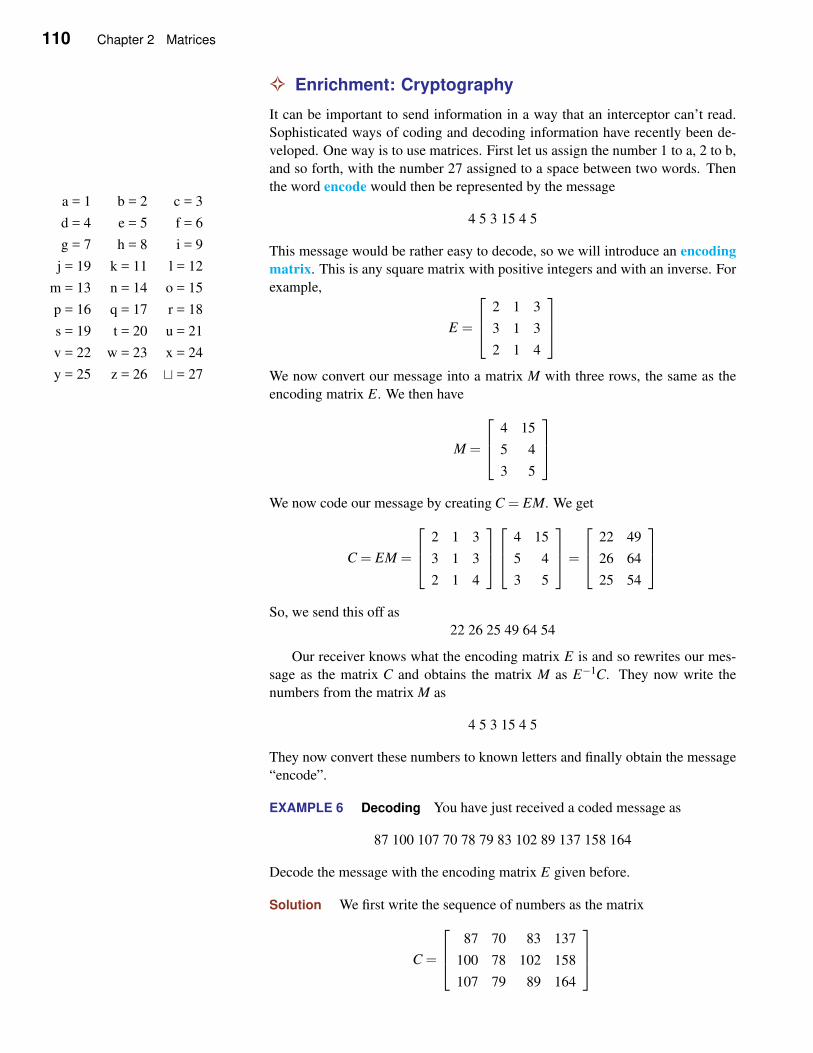
110 Chapter 2 Matrices
✧ Enrichment: Cryptography
It can be important to send information in a way that an interceptor can’t read.
Sophisticated ways of coding and decoding information have recently been de-
veloped. One way is to use matrices. First let us assign the number 1 to a, 2 to b,
and so forth, with the number 27 assigned to a space between two words. Then
the word encode would then be represented by the message
4 5 3 15 4 5
This message would be rather easy to decode, so we will introduce an encoding
matrix. This is any square matrix with positive integers and with an inverse. For
example,
a = 1 b = 2 c = 3
d = 4 e = 5 f = 6
g = 7 h = 8 i = 9
j = 19 k = 11 l = 12
m = 13 n = 14 o = 15
p = 16 q = 17 r = 18
s = 19 t = 20 u = 21
v = 22 w = 23 x = 24
y = 25 z = 26 ⊔ = 27
E =
2 1 3
3 1 3
2 1 4
We now convert our message into a matrix M with three rows, the same as the
encoding matrix E. We then have
M =
4 15
5 4
3 5
We now code our message by creating C = EM. We get
C = EM =
2 1 3
3 1 3
2 1 4
4 15
5 4
3 5
=
22 49
26 64
25 54
So, we send this off as
22 26 25 49 64 54
Our receiver knows what the encoding matrix E is and so rewrites our mes-
sage as the matrix C and obtains the matrix M as E−1C. They now write the
numbers from the matrix M as
4 5 3 15 4 5
They now convert these numbers to known letters and finally obtain the message
“encode”.
EXAMPLE 6 Decoding You have just received a coded message as
87 100 107 70 78 79 83 102 89 137 158 164
Decode the message with the encoding matrix E given before.
Solution We first write the sequence of numbers as the matrix
C =
87 70 83 137
100 78 102 158
107 79 89 164
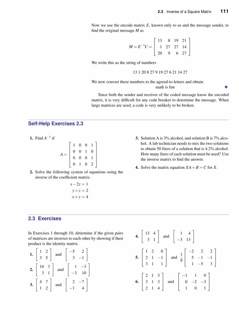
2.3 Inverse of a Square Matrix 111
Now we use the encode matrix E, known only to us and the message sender, to
find the original message M as
M = E−1C =
13 8 19 21
1 27 27 14
20 9 6 27
We write this as the string of numbers
13 1 20 8 27 9 19 27 6 21 14 27
We now convert these numbers to the agreed-to-letters and obtain
math is fun ✦
Since both the sender and receiver of the coded message know the encoded
matrix, it is very difficult for any code breaker to determine the message. When
large matrices are used, a code is very unlikely to be broken.
Self-Help Exercises 2.3
1. Find A−1 if
A =
1 0 0 1
0 0 1 0
0 0 0 1
0 1 0 2
2. Solve the following system of equations using the
inverse of the coefficient matrix:
x−2z = 1
y+ z = 2
x+ y = 4
3. Solution A is 3% alcohol, and solution B is 7% alco-
hol. A lab technician needs to mix the two solutions
to obtain 50 liters of a solution that is 4.2% alcohol.
How many liters of each solution must be used? Use
the inverse matrix to find the answer.
4. Solve the matrix equation XA+B =C for X .
2.3 Exercises
In Exercises 1 through 10, determine if the given pairs
of matrices are inverses to each other by showing if their
product is the identity matrix.
1.
[
1 2
3 5
]
and
[
−5 2
3 −1
]
2.
[
10 3
3 1
]
and
[
1 −3
−3 10
]
3.
[
4 7
1 2
]
and
[
2 −7
−1 4
]
4.
[
13 4
3 1
]
and
[
1 4
−3 13
]
5.
1 2 0
2 1 −1
3 1 1
and
1
8
−2 2 2
5 −1 −1
1 −5 3
6.
2 1 3
3 1 3
2 1 4
and
−1 1 0
0 −2 −3
1 0 1
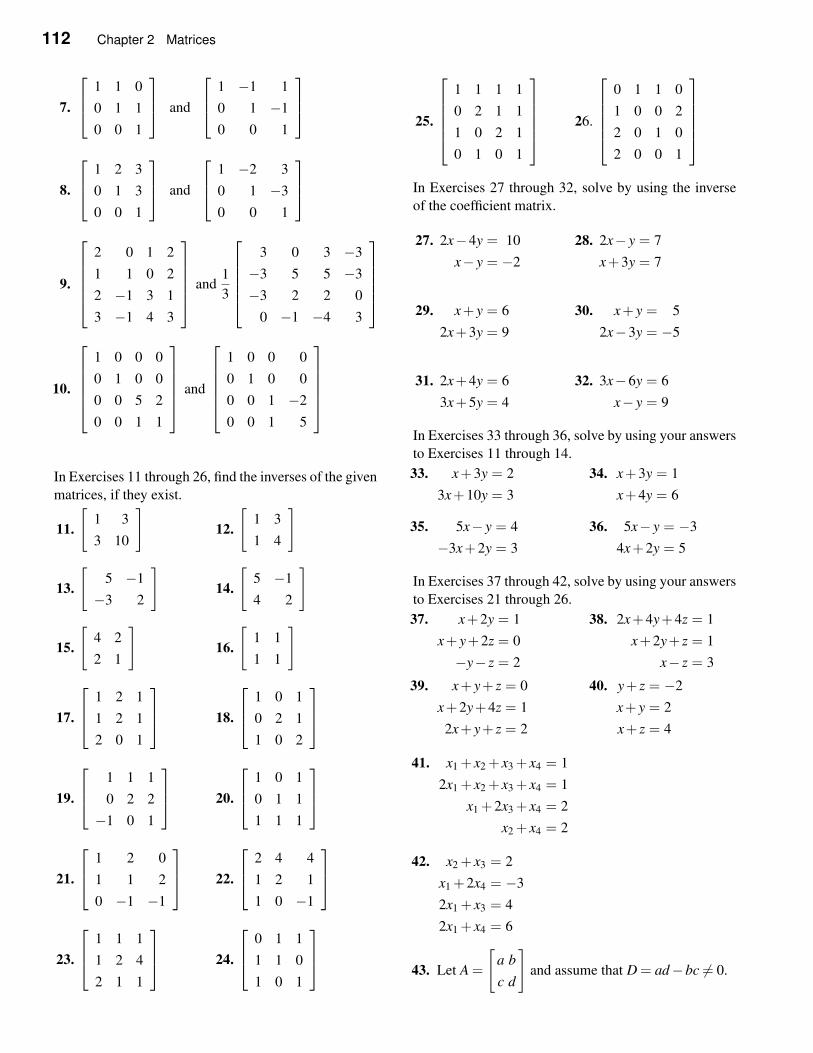
112 Chapter 2 Matrices
7.
1 1 0
0 1 1
0 0 1
and
1 −1 1
0 1 −1
0 0 1
8.
1 2 3
0 1 3
0 0 1
and
1 −2 3
0 1 −3
0 0 1
9.
2 0 1 2
1 1 0 2
2 −1 3 1
3 −1 4 3
and1
3
3 0 3 −3
−3 5 5 −3
−3 2 2 0
0 −1 −4 3
10.
1 0 0 0
0 1 0 0
0 0 5 2
0 0 1 1
and
1 0 0 0
0 1 0 0
0 0 1 −2
0 0 1 5
In Exercises 11 through 26, find the inverses of the given
matrices, if they exist.
11.
[
1 3
3 10
]
12.
[
1 3
1 4
]
13.
[
5 −1
−3 2
]
14.
[
5 −1
4 2
]
15.
[
4 2
2 1
]
16.
[
1 1
1 1
]
17.
1 2 1
1 2 1
2 0 1
18.
1 0 1
0 2 1
1 0 2
19.
1 1 1
0 2 2
−1 0 1
20.
1 0 1
0 1 1
1 1 1
21.
1 2 0
1 1 2
0 −1 −1
22.
2 4 4
1 2 1
1 0 −1
23.
1 1 1
1 2 4
2 1 1
24.
0 1 1
1 1 0
1 0 1
25.
1 1 1 1
0 2 1 1
1 0 2 1
0 1 0 1
26.
0 1 1 0
1 0 0 2
2 0 1 0
2 0 0 1
In Exercises 27 through 32, solve by using the inverse
of the coefficient matrix.
27. 2x−4y = 10
x− y = −2
28. 2x− y = 7
x+3y = 7
29. x+ y = 6
2x+3y = 9
30. x+ y = 5
2x−3y = −5
31. 2x+4y = 6
3x+5y = 4
32. 3x−6y = 6
x− y = 9
In Exercises 33 through 36, solve by using your answers
to Exercises 11 through 14.
33. x+3y = 2
3x+10y = 3
34. x+3y = 1
x+4y = 6
35. 5x− y = 4
−3x+2y = 3
36. 5x− y = −3
4x+2y = 5
In Exercises 37 through 42, solve by using your answers
to Exercises 21 through 26.
37. x+2y = 1
x+ y+2z = 0
−y− z = 2
38. 2x+4y+4z = 1
x+2y+ z = 1
x− z = 3
39. x+ y+ z = 0
x+2y+4z = 1
2x+ y+ z = 2
40. y+ z = −2
x+ y = 2
x+ z = 4
41. x1 + x2 + x3 + x4 = 1
2x1 + x2 + x3 + x4 = 1
x1 +2x3 + x4 = 2
x2 + x4 = 2
42. x2 + x3 = 2
x1 +2x4 = −3
2x1 + x3 = 4
2x1 + x4 = 6
43. Let A =
[
a b
c d
]
and assume that D = ad−bc 6= 0.
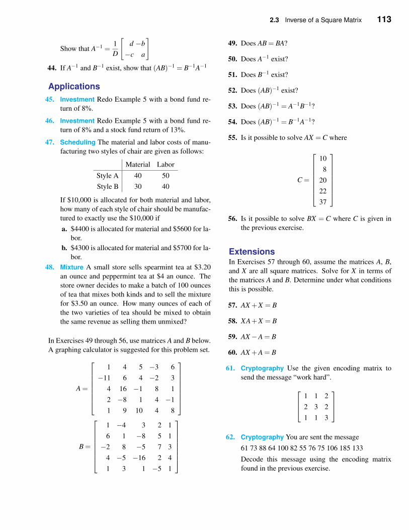
2.3 Inverse of a Square Matrix 113
Show that A−1 =1
D
[
d −b
−c a
]
44. If A−1 and B−1 exist, show that (AB)−1 = B−1A−1
Applications
45. Investment Redo Example 5 with a bond fund re-
turn of 8%.
46. Investment Redo Example 5 with a bond fund re-
turn of 8% and a stock fund return of 13%.
47. Scheduling The material and labor costs of manu-
facturing two styles of chair are given as follows:
Material Labor
Style A 40 50
Style B 30 40
If $10,000 is allocated for both material and labor,
how many of each style of chair should be manufac-
tured to exactly use the $10,000 if
a. $4400 is allocated for material and $5600 for la-
bor.
b. $4300 is allocated for material and $5700 for la-
bor.
48. Mixture A small store sells spearmint tea at $3.20
an ounce and peppermint tea at $4 an ounce. The
store owner decides to make a batch of 100 ounces
of tea that mixes both kinds and to sell the mixture
for $3.50 an ounce. How many ounces of each of
the two varieties of tea should be mixed to obtain
the same revenue as selling them unmixed?
In Exercises 49 through 56, use matrices A and B below.
A graphing calculator is suggested for this problem set.
A =
1 4 5 −3 6
−11 6 4 −2 3
4 16 −1 8 1
2 −8 1 4 −1
1 9 10 4 8
B =
1 −4 3 2 1
6 1 −8 5 1
−2 8 −5 7 3
4 −5 −16 2 4
1 3 1 −5 1
49. Does AB = BA?
50. Does A−1 exist?
51. Does B−1 exist?
52. Does (AB)−1 exist?
53. Does (AB)−1 = A−1B−1?
54. Does (AB)−1 = B−1A−1?
55. Is it possible to solve AX =C where
C =
10
8
20
22
37
56. Is it possible to solve BX = C where C is given in
the previous exercise.
ExtensionsIn Exercises 57 through 60, assume the matrices A, B,
and X are all square matrices. Solve for X in terms of
the matrices A and B. Determine under what conditions
this is possible.
57. AX +X = B
58. XA+X = B
59. AX−A = B
60. AX +A = B
61. Cryptography Use the given encoding matrix to
send the message “work hard”.
1 1 2
2 3 2
1 1 3
62. Cryptography You are sent the message
61 73 88 64 100 82 55 76 75 106 185 133
Decode this message using the encoding matrix
found in the previous exercise.
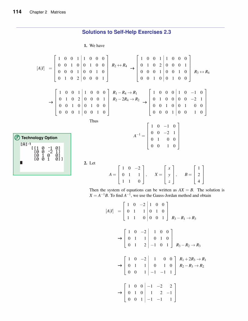
114 Chapter 2 Matrices
Solutions to Self-Help Exercises 2.3
1. We have
[A|I] =
1 0 0 1 1 0 0 0
0 0 1 0 0 1 0 0
0 0 0 1 0 0 1 0
0 1 0 2 0 0 0 1
R2↔ R4 →→→
1 0 0 1 1 0 0 0
0 1 0 2 0 0 0 1
0 0 0 1 0 0 1 0
0 0 1 0 0 1 0 0
R3↔ R4
→→→
1 0 0 1 1 0 0 0
0 1 0 2 0 0 0 1
0 0 1 0 0 1 0 0
0 0 0 1 0 0 1 0
R1−R4→ R1
R2−2R4→ R2 →→→
1 0 0 0 1 0 −1 0
0 1 0 0 0 0 −2 1
0 0 1 0 0 1 0 0
0 0 0 1 0 0 1 0
Thus
A−1 =
1 0 −1 0
0 0 −2 1
0 1 0 0
0 0 1 0
TTT©©© Technology Option
2. Let
A =
1 0 −2
0 1 1
1 1 0
, X =
x
y
z
, B =
1
2
4
Then the system of equations can be written as AX = B. The solution is
X = A−1B. To find A−1, we use the Gauss-Jordan method and obtain
[A|I] =
1 0 −2 1 0 0
0 1 1 0 1 0
1 1 0 0 0 1
R3−R1→ R3
→→→
1 0 −2 1 0 0
0 1 1 0 1 0
0 1 2 −1 0 1
R3−R2→ R3
→→→
1 0 −2 1 0 0
0 1 1 0 1 0
0 0 1 −1 −1 1
R1 +2R3→ R1
R2−R3→ R2
→→→
1 0 0 −1 −2 2
0 1 0 1 2 −1
0 0 1 −1 −1 1
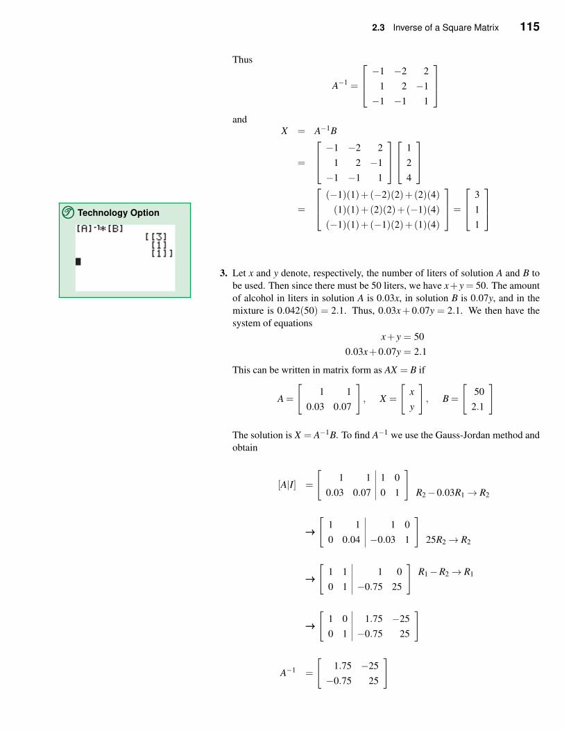
2.3 Inverse of a Square Matrix 115
Thus
A−1 =
−1 −2 2
1 2 −1
−1 −1 1
andX = A−1B
=
−1 −2 2
1 2 −1
−1 −1 1
1
2
4
=
(−1)(1)+(−2)(2)+(2)(4)
(1)(1)+(2)(2)+(−1)(4)
(−1)(1)+(−1)(2)+(1)(4)
=
3
1
1
TTT©©© Technology Option
3. Let x and y denote, respectively, the number of liters of solution A and B to
be used. Then since there must be 50 liters, we have x+y = 50. The amount
of alcohol in liters in solution A is 0.03x, in solution B is 0.07y, and in the
mixture is 0.042(50) = 2.1. Thus, 0.03x+ 0.07y = 2.1. We then have the
system of equations
x+ y = 50
0.03x+0.07y = 2.1
This can be written in matrix form as AX = B if
A =
[
1 1
0.03 0.07
]
, X =
[
x
y
]
, B =
[
50
2.1
]
The solution is X = A−1B. To find A−1 we use the Gauss-Jordan method and
obtain
[A|I] =
[
1 1 1 0
0.03 0.07 0 1
]
R2−0.03R1→ R2
→→→[
1 1 1 0
0 0.04 −0.03 1
]
25R2→ R2
→→→[
1 1 1 0
0 1 −0.75 25
]
R1−R2→ R1
→→→[
1 0 1.75 −25
0 1 −0.75 25
]
A−1 =
[
1.75 −25
−0.75 25
]
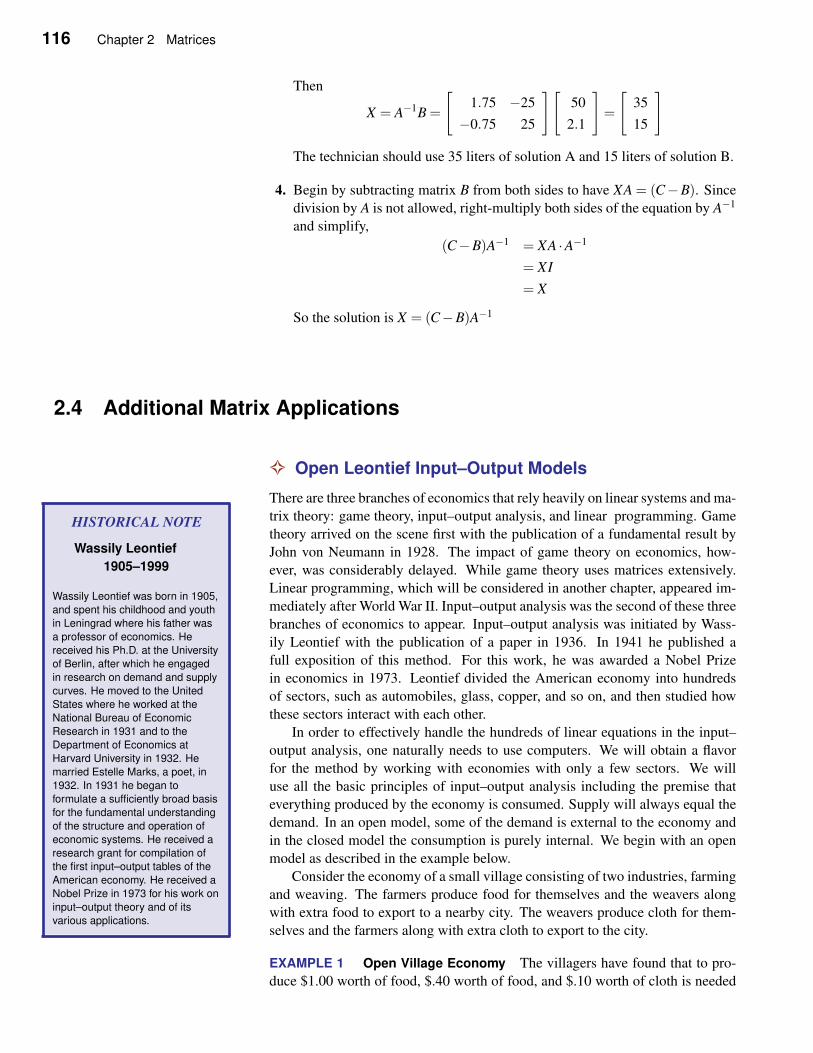
116 Chapter 2 Matrices
Then
X = A−1B =
[
1.75 −25
−0.75 25
][
50
2.1
]
=
[
35
15
]
The technician should use 35 liters of solution A and 15 liters of solution B.
4. Begin by subtracting matrix B from both sides to have XA = (C−B). Since
division by A is not allowed, right-multiply both sides of the equation by A−1
and simplify,
(C−B)A−1 = XA ·A−1
= XI
= X
So the solution is X = (C−B)A−1
2.4 Additional Matrix Applications
✧ Open Leontief Input–Output Models
There are three branches of economics that rely heavily on linear systems and ma-
trix theory: game theory, input–output analysis, and linear programming. GameHISTORICAL NOTE
Wassily Leontief
1905–1999
Wassily Leontief was born in 1905,
and spent his childhood and youth
in Leningrad where his father was
a professor of economics. He
received his Ph.D. at the University
of Berlin, after which he engaged
in research on demand and supply
curves. He moved to the United
States where he worked at the
National Bureau of Economic
Research in 1931 and to the
Department of Economics at
Harvard University in 1932. He
married Estelle Marks, a poet, in
1932. In 1931 he began to
formulate a sufficiently broad basis
for the fundamental understanding
of the structure and operation of
economic systems. He received a
research grant for compilation of
the first input–output tables of the
American economy. He received a
Nobel Prize in 1973 for his work on
input–output theory and of its
various applications.
theory arrived on the scene first with the publication of a fundamental result by
John von Neumann in 1928. The impact of game theory on economics, how-
ever, was considerably delayed. While game theory uses matrices extensively.
Linear programming, which will be considered in another chapter, appeared im-
mediately after World War II. Input–output analysis was the second of these three
branches of economics to appear. Input–output analysis was initiated by Wass-
ily Leontief with the publication of a paper in 1936. In 1941 he published a
full exposition of this method. For this work, he was awarded a Nobel Prize
in economics in 1973. Leontief divided the American economy into hundreds
of sectors, such as automobiles, glass, copper, and so on, and then studied how
these sectors interact with each other.
In order to effectively handle the hundreds of linear equations in the input–
output analysis, one naturally needs to use computers. We will obtain a flavor
for the method by working with economies with only a few sectors. We will
use all the basic principles of input–output analysis including the premise that
everything produced by the economy is consumed. Supply will always equal the
demand. In an open model, some of the demand is external to the economy and
in the closed model the consumption is purely internal. We begin with an open
model as described in the example below.
Consider the economy of a small village consisting of two industries, farming
and weaving. The farmers produce food for themselves and the weavers along
with extra food to export to a nearby city. The weavers produce cloth for them-
selves and the farmers along with extra cloth to export to the city.
EXAMPLE 1 Open Village Economy The villagers have found that to pro-
duce $1.00 worth of food, $.40 worth of food, and $.10 worth of cloth is needed
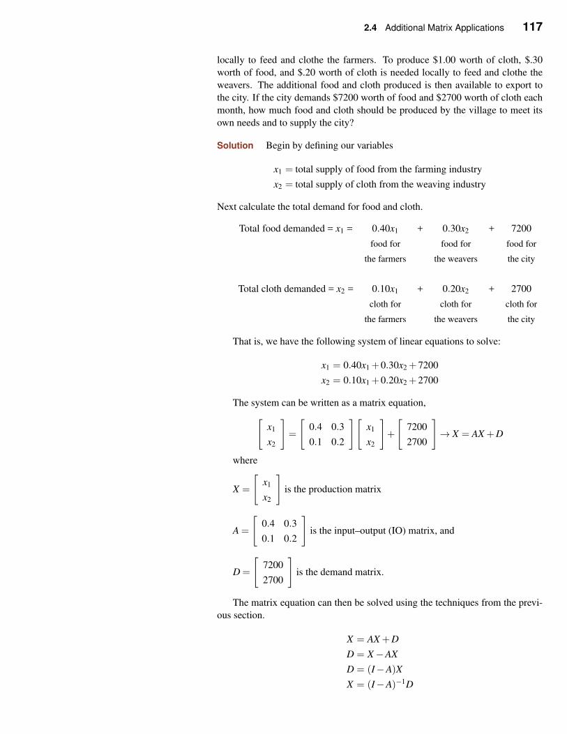
2.4 Additional Matrix Applications 117
locally to feed and clothe the farmers. To produce $1.00 worth of cloth, $.30
worth of food, and $.20 worth of cloth is needed locally to feed and clothe the
weavers. The additional food and cloth produced is then available to export to
the city. If the city demands $7200 worth of food and $2700 worth of cloth each
month, how much food and cloth should be produced by the village to meet its
own needs and to supply the city?
Solution Begin by defining our variables
x1 = total supply of food from the farming industry
x2 = total supply of cloth from the weaving industry
Next calculate the total demand for food and cloth.
Total food demanded = x1 = 0.40x1 + 0.30x2 + 7200
food for food for food for
the farmers the weavers the city
Total cloth demanded = x2 = 0.10x1 + 0.20x2 + 2700
cloth for cloth for cloth for
the farmers the weavers the city
That is, we have the following system of linear equations to solve:
x1 = 0.40x1 +0.30x2 +7200
x2 = 0.10x1 +0.20x2 +2700
The system can be written as a matrix equation,
[
x1
x2
]
=
[
0.4 0.3
0.1 0.2
][
x1
x2
]
+
[
7200
2700
]
→ X = AX +D
where
X =
[
x1
x2
]
is the production matrix
A =
[
0.4 0.3
0.1 0.2
]
is the input–output (IO) matrix, and
D =
[
7200
2700
]
is the demand matrix.
The matrix equation can then be solved using the techniques from the previ-
ous section.
X = AX +D
D = X−AX
D = (I−A)X
X = (I−A)−1D
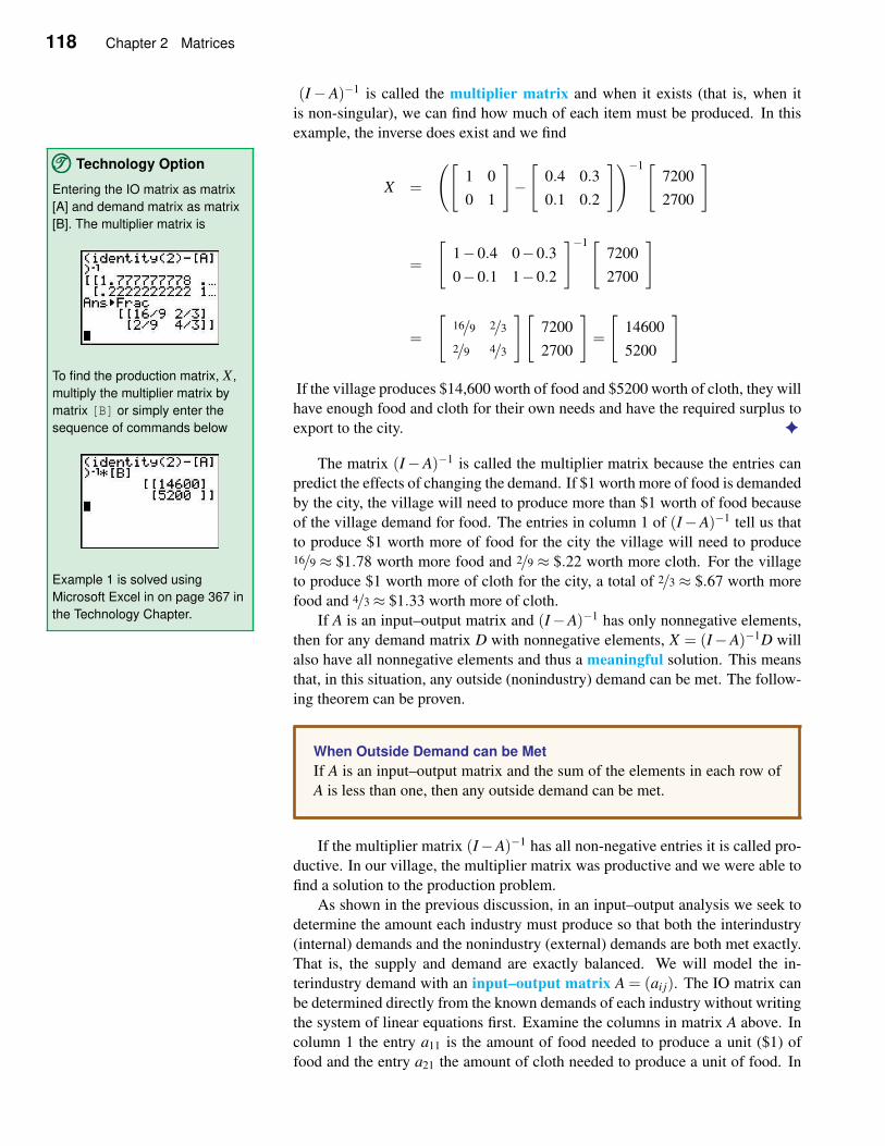
118 Chapter 2 Matrices
(I−A)−1 is called the multiplier matrix and when it exists (that is, when it
is non-singular), we can find how much of each item must be produced. In this
example, the inverse does exist and we find
X =
([
1 0
0 1
]
−[
0.4 0.3
0.1 0.2
])−1[
7200
2700
]
=
[
1−0.4 0−0.3
0−0.1 1−0.2
]−1[
7200
2700
]
=
[
16/9 2/3
2/9 4/3
][
7200
2700
]
=
[
14600
5200
]
If the village produces $14,600 worth of food and $5200 worth of cloth, they will
TTT©©© Technology Option
Entering the IO matrix as matrix
[A] and demand matrix as matrix
[B]. The multiplier matrix is
To find the production matrix, X ,
multiply the multiplier matrix by
matrix [B] or simply enter the
sequence of commands below
Example 1 is solved using
Microsoft Excel in on page 367 in
the Technology Chapter.
have enough food and cloth for their own needs and have the required surplus to
export to the city. ✦
The matrix (I−A)−1 is called the multiplier matrix because the entries can
predict the effects of changing the demand. If $1 worth more of food is demanded
by the city, the village will need to produce more than $1 worth of food because
of the village demand for food. The entries in column 1 of (I−A)−1 tell us that
to produce $1 worth more of food for the city the village will need to produce16/9 ≈ $1.78 worth more food and 2/9 ≈ $.22 worth more cloth. For the village
to produce $1 worth more of cloth for the city, a total of 2/3 ≈ $.67 worth more
food and 4/3≈ $1.33 worth more of cloth.
If A is an input–output matrix and (I−A)−1 has only nonnegative elements,
then for any demand matrix D with nonnegative elements, X = (I−A)−1D will
also have all nonnegative elements and thus a meaningful solution. This means
that, in this situation, any outside (nonindustry) demand can be met. The follow-
ing theorem can be proven.
When Outside Demand can be Met
If A is an input–output matrix and the sum of the elements in each row of
A is less than one, then any outside demand can be met.
If the multiplier matrix (I−A)−1 has all non-negative entries it is called pro-
ductive. In our village, the multiplier matrix was productive and we were able to
find a solution to the production problem.
As shown in the previous discussion, in an input–output analysis we seek to
determine the amount each industry must produce so that both the interindustry
(internal) demands and the nonindustry (external) demands are both met exactly.
That is, the supply and demand are exactly balanced. We will model the in-
terindustry demand with an input–output matrix A = (ai j). The IO matrix can
be determined directly from the known demands of each industry without writing
the system of linear equations first. Examine the columns in matrix A above. In
column 1 the entry a11 is the amount of food needed to produce a unit ($1) of
food and the entry a21 the amount of cloth needed to produce a unit of food. In
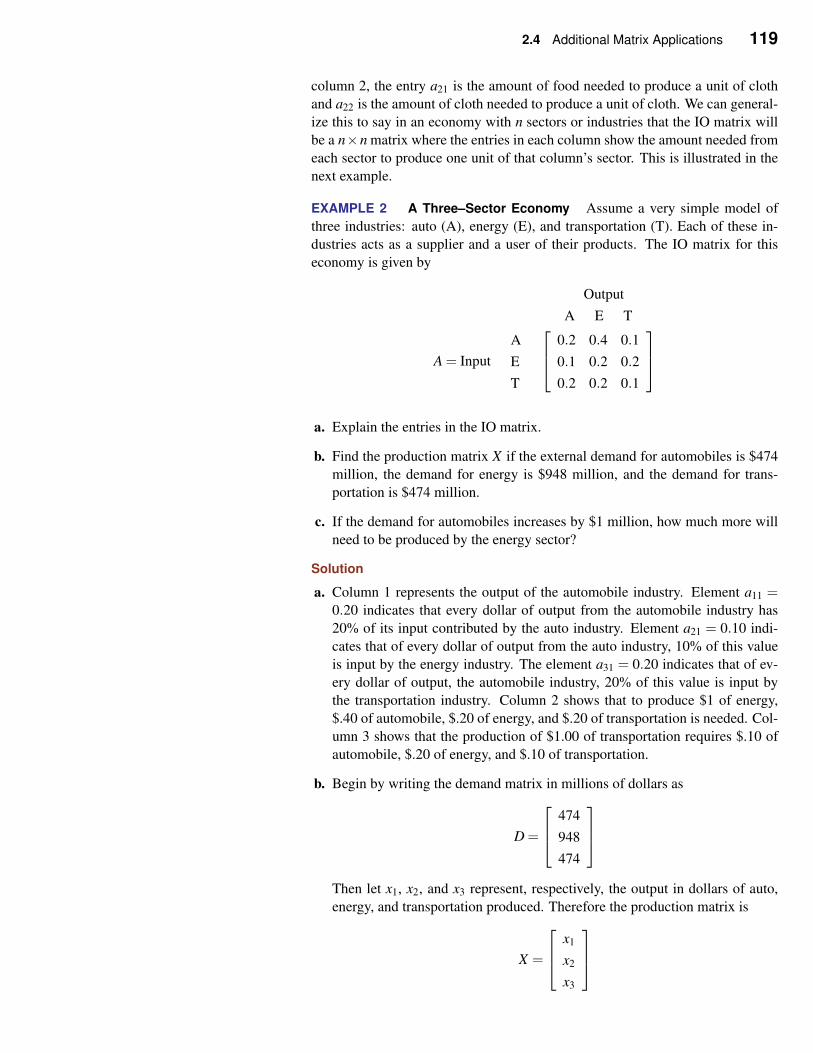
2.4 Additional Matrix Applications 119
column 2, the entry a21 is the amount of food needed to produce a unit of cloth
and a22 is the amount of cloth needed to produce a unit of cloth. We can general-
ize this to say in an economy with n sectors or industries that the IO matrix will
be a n×n matrix where the entries in each column show the amount needed from
each sector to produce one unit of that column’s sector. This is illustrated in the
next example.
EXAMPLE 2 A Three–Sector Economy Assume a very simple model of
three industries: auto (A), energy (E), and transportation (T). Each of these in-
dustries acts as a supplier and a user of their products. The IO matrix for this
economy is given by
Output
A E T
A = Input
A
E
T
0.2 0.4 0.1
0.1 0.2 0.2
0.2 0.2 0.1
a. Explain the entries in the IO matrix.
b. Find the production matrix X if the external demand for automobiles is $474
million, the demand for energy is $948 million, and the demand for trans-
portation is $474 million.
c. If the demand for automobiles increases by $1 million, how much more will
need to be produced by the energy sector?
Solution
a. Column 1 represents the output of the automobile industry. Element a11 =0.20 indicates that every dollar of output from the automobile industry has
20% of its input contributed by the auto industry. Element a21 = 0.10 indi-
cates that of every dollar of output from the auto industry, 10% of this value
is input by the energy industry. The element a31 = 0.20 indicates that of ev-
ery dollar of output, the automobile industry, 20% of this value is input by
the transportation industry. Column 2 shows that to produce $1 of energy,
$.40 of automobile, $.20 of energy, and $.20 of transportation is needed. Col-
umn 3 shows that the production of $1.00 of transportation requires $.10 of
automobile, $.20 of energy, and $.10 of transportation.
b. Begin by writing the demand matrix in millions of dollars as
D =
474
948
474
Then let x1, x2, and x3 represent, respectively, the output in dollars of auto,
energy, and transportation produced. Therefore the production matrix is
X =
x1
x2
x3
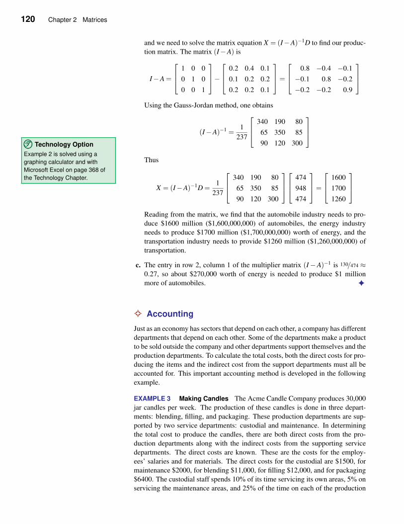
120 Chapter 2 Matrices
and we need to solve the matrix equation X = (I−A)−1D to find our produc-
tion matrix. The matrix (I−A) is
I−A =
1 0 0
0 1 0
0 0 1
−
0.2 0.4 0.1
0.1 0.2 0.2
0.2 0.2 0.1
=
0.8 −0.4 −0.1
−0.1 0.8 −0.2
−0.2 −0.2 0.9
Using the Gauss-Jordan method, one obtains
(I−A)−1 =1
237
340 190 80
65 350 85
90 120 300
Thus
TTT©©© Technology Option
Example 2 is solved using a
graphing calculator and with
Microsoft Excel on page 368 of
the Technology Chapter.
X = (I−A)−1D =1
237
340 190 80
65 350 85
90 120 300
474
948
474
=
1600
1700
1260
Reading from the matrix, we find that the automobile industry needs to pro-
duce $1600 million ($1,600,000,000) of automobiles, the energy industry
needs to produce $1700 million ($1,700,000,000) worth of energy, and the
transportation industry needs to provide $1260 million ($1,260,000,000) of
transportation.
c. The entry in row 2, column 1 of the multiplier matrix (I−A)−1 is 130/474 ≈0.27, so about $270,000 worth of energy is needed to produce $1 million
more of automobiles. ✦
✧ Accounting
Just as an economy has sectors that depend on each other, a company has different
departments that depend on each other. Some of the departments make a product
to be sold outside the company and other departments support themselves and the
production departments. To calculate the total costs, both the direct costs for pro-
ducing the items and the indirect cost from the support departments must all be
accounted for. This important accounting method is developed in the following
example.
EXAMPLE 3 Making Candles The Acme Candle Company produces 30,000
jar candles per week. The production of these candles is done in three depart-
ments: blending, filling, and packaging. These production departments are sup-
ported by two service departments: custodial and maintenance. In determining
the total cost to produce the candles, there are both direct costs from the pro-
duction departments along with the indirect costs from the supporting service
departments. The direct costs are known. These are the costs for the employ-
ees’ salaries and for materials. The direct costs for the custodial are $1500, for
maintenance $2000, for blending $11,000, for filling $12,000, and for packaging
$6400. The custodial staff spends 10% of its time servicing its own areas, 5% on
servicing the maintenance areas, and 25% of the time on each of the production
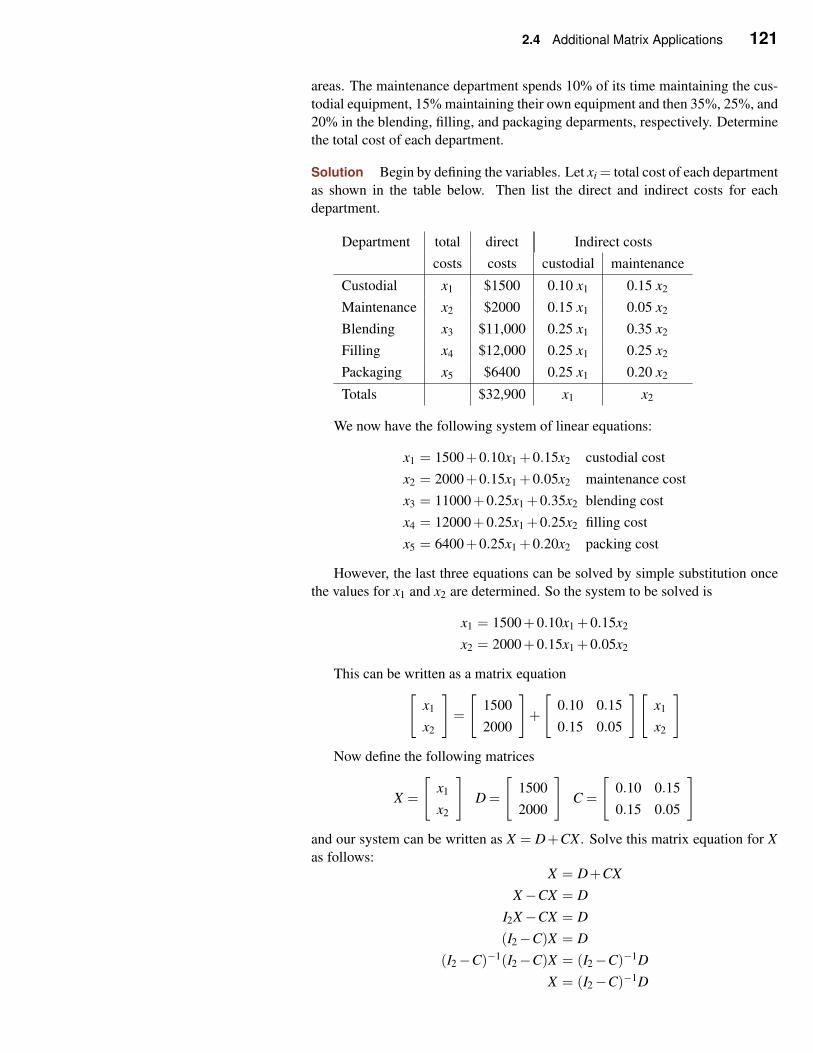
2.4 Additional Matrix Applications 121
areas. The maintenance department spends 10% of its time maintaining the cus-
todial equipment, 15% maintaining their own equipment and then 35%, 25%, and
20% in the blending, filling, and packaging deparments, respectively. Determine
the total cost of each department.
Solution Begin by defining the variables. Let xi = total cost of each department
as shown in the table below. Then list the direct and indirect costs for each
department.
Department total direct Indirect costs
costs costs custodial maintenance
Custodial x1 $1500 0.10 x1 0.15 x2
Maintenance x2 $2000 0.15 x1 0.05 x2
Blending x3 $11,000 0.25 x1 0.35 x2
Filling x4 $12,000 0.25 x1 0.25 x2
Packaging x5 $6400 0.25 x1 0.20 x2
Totals $32,900 x1 x2
We now have the following system of linear equations:
x1 = 1500+0.10x1 +0.15x2 custodial cost
x2 = 2000+0.15x1 +0.05x2 maintenance cost
x3 = 11000+0.25x1 +0.35x2 blending cost
x4 = 12000+0.25x1 +0.25x2 filling cost
x5 = 6400+0.25x1 +0.20x2 packing cost
However, the last three equations can be solved by simple substitution once
the values for x1 and x2 are determined. So the system to be solved is
x1 = 1500+0.10x1 +0.15x2
x2 = 2000+0.15x1 +0.05x2
This can be written as a matrix equation[
x1
x2
]
=
[
1500
2000
]
+
[
0.10 0.15
0.15 0.05
][
x1
x2
]
Now define the following matrices
X =
[
x1
x2
]
D =
[
1500
2000
]
C =
[
0.10 0.15
0.15 0.05
]
and our system can be written as X = D+CX . Solve this matrix equation for X
as follows:X = D+CX
X−CX = D
I2X−CX = D
(I2−C)X = D
(I2−C)−1(I2−C)X = (I2−C)−1D
X = (I2−C)−1D
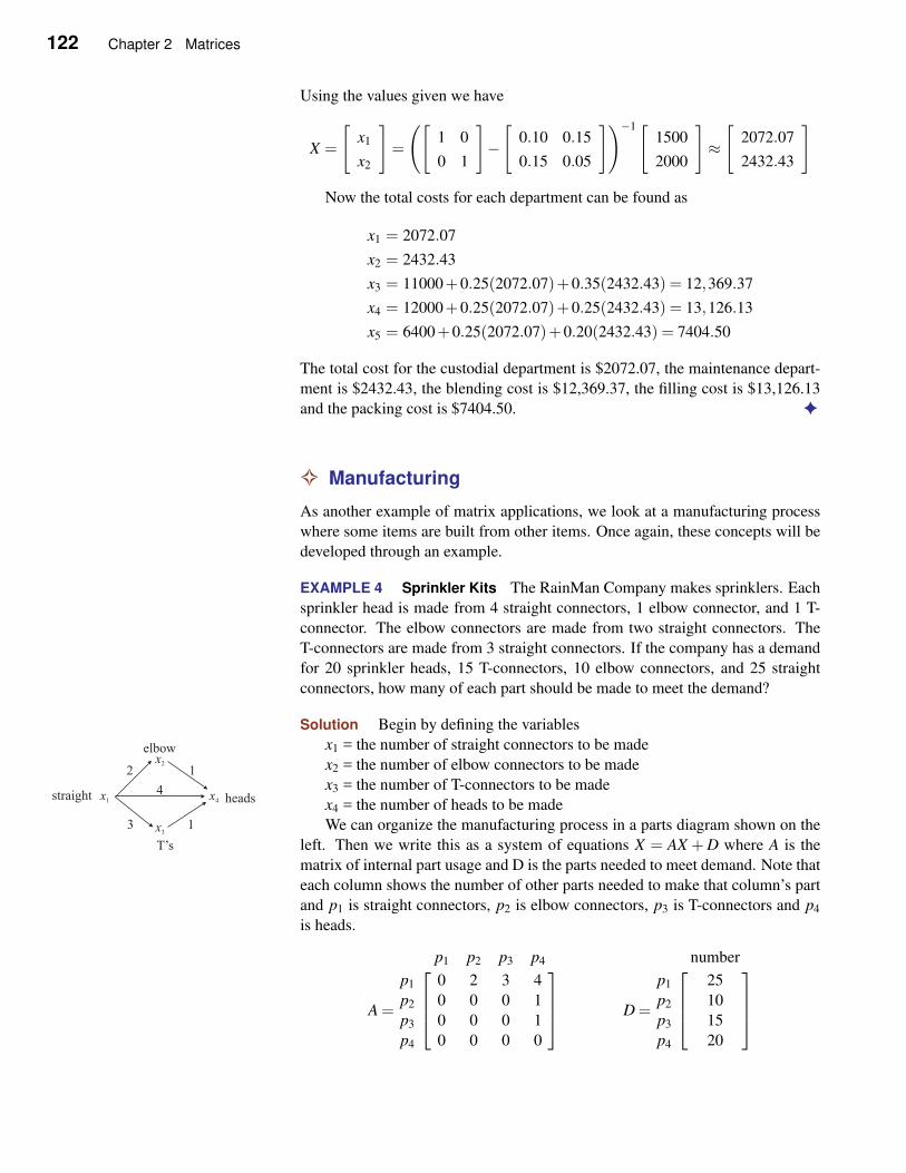
122 Chapter 2 Matrices
Using the values given we have
X =
[
x1
x2
]
=
([
1 0
0 1
]
−[
0.10 0.15
0.15 0.05
])−1[
1500
2000
]
≈[
2072.07
2432.43
]
Now the total costs for each department can be found as
x1 = 2072.07
x2 = 2432.43
x3 = 11000+0.25(2072.07)+0.35(2432.43) = 12,369.37
x4 = 12000+0.25(2072.07)+0.25(2432.43) = 13,126.13
x5 = 6400+0.25(2072.07)+0.20(2432.43) = 7404.50
The total cost for the custodial department is $2072.07, the maintenance depart-
ment is $2432.43, the blending cost is $12,369.37, the filling cost is $13,126.13
and the packing cost is $7404.50. ✦
✧ Manufacturing
As another example of matrix applications, we look at a manufacturing process
where some items are built from other items. Once again, these concepts will be
developed through an example.
EXAMPLE 4 Sprinkler Kits The RainMan Company makes sprinklers. Each
sprinkler head is made from 4 straight connectors, 1 elbow connector, and 1 T-
connector. The elbow connectors are made from two straight connectors. The
T-connectors are made from 3 straight connectors. If the company has a demand
for 20 sprinkler heads, 15 T-connectors, 10 elbow connectors, and 25 straight
connectors, how many of each part should be made to meet the demand?
Solution Begin by defining the variables
x1 = the number of straight connectors to be made
x2 = the number of elbow connectors to be made
x3 = the number of T-connectors to be made
x4 = the number of heads to be made
We can organize the manufacturing process in a parts diagram shown on the
left. Then we write this as a system of equations X = AX +D where A is the
matrix of internal part usage and D is the parts needed to meet demand. Note that
each column shows the number of other parts needed to make that column’s part
and p1 is straight connectors, p2 is elbow connectors, p3 is T-connectors and p4
is heads.
A =
p1 p2 p3 p4
p1 0 2 3 4
p2 0 0 0 1
p3 0 0 0 1
p4 0 0 0 0
D =
number
p1 25
p2 10
p3 15
p4 20
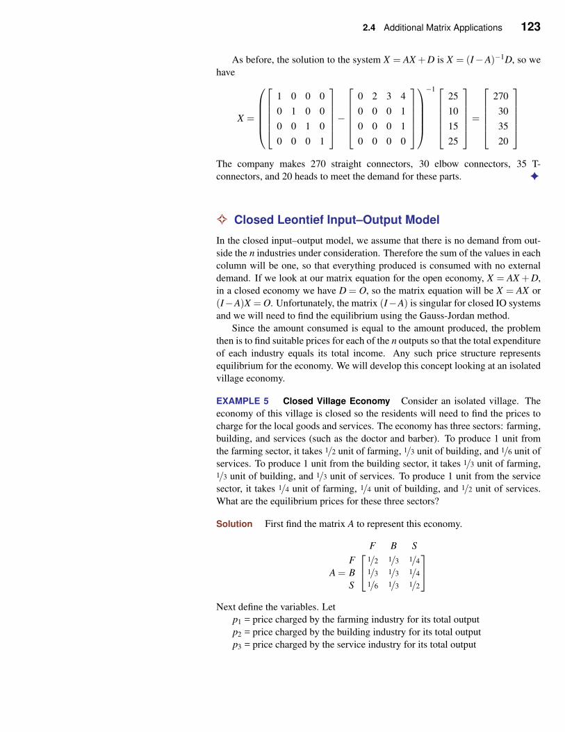
2.4 Additional Matrix Applications 123
As before, the solution to the system X = AX +D is X = (I−A)−1D, so we
have
X =
1 0 0 0
0 1 0 0
0 0 1 0
0 0 0 1
−
0 2 3 4
0 0 0 1
0 0 0 1
0 0 0 0
−1
25
10
15
25
=
270
30
35
20
The company makes 270 straight connectors, 30 elbow connectors, 35 T-
connectors, and 20 heads to meet the demand for these parts. ✦
✧ Closed Leontief Input–Output Model
In the closed input–output model, we assume that there is no demand from out-
side the n industries under consideration. Therefore the sum of the values in each
column will be one, so that everything produced is consumed with no external
demand. If we look at our matrix equation for the open economy, X = AX +D,
in a closed economy we have D = O, so the matrix equation will be X = AX or
(I−A)X = O. Unfortunately, the matrix (I−A) is singular for closed IO systems
and we will need to find the equilibrium using the Gauss-Jordan method.
Since the amount consumed is equal to the amount produced, the problem
then is to find suitable prices for each of the n outputs so that the total expenditure
of each industry equals its total income. Any such price structure represents
equilibrium for the economy. We will develop this concept looking at an isolated
village economy.
EXAMPLE 5 Closed Village Economy Consider an isolated village. The
economy of this village is closed so the residents will need to find the prices to
charge for the local goods and services. The economy has three sectors: farming,
building, and services (such as the doctor and barber). To produce 1 unit from
the farming sector, it takes 1/2 unit of farming, 1/3 unit of building, and 1/6 unit of
services. To produce 1 unit from the building sector, it takes 1/3 unit of farming,1/3 unit of building, and 1/3 unit of services. To produce 1 unit from the service
sector, it takes 1/4 unit of farming, 1/4 unit of building, and 1/2 unit of services.
What are the equilibrium prices for these three sectors?
Solution First find the matrix A to represent this economy.
A =
F B S
F 1/2 1/3 1/4
B 1/3 1/3 1/4
S 1/6 1/3 1/2
Next define the variables. Let
p1 = price charged by the farming industry for its total output
p2 = price charged by the building industry for its total output
p3 = price charged by the service industry for its total output
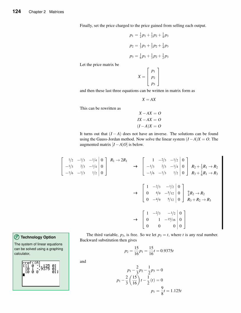
124 Chapter 2 Matrices
Finally, set the price charged to the price gained from selling each output.
p1 = 12 p1 +
13 p2 +
14 p3
p2 = 13 p1 +
13 p2 +
14 p3
p3 = 16 p1 +
13 p2 +
12 p3
Let the price matrix be
X =
p1
p2
p3
and then these last three equations can be written in matrix form as
X = AX
This can be rewritten asX−AX = O
IX−AX = O
(I−A)X = O
It turns out that (I−A) does not have an inverse. The solutions can be found
using the Gauss-Jordan method. Now solve the linear system (I−A)X = O. The
augmented matrix [I−A|O] is below.
1/2 −1/3 −1/4 0
−1/3 2/3 −1/4 0
−1/6 −1/3 1/2 0
R1→ 2R1
→→→
1 −2/3 −1/2 0
−1/3 2/3 −1/4 0
−1/6 −1/3 1/2 0
R2 +
13 R1→ R2
R3 +16 R1→ R3
→→→
1 −2/3 −1/2 0
0 4/9 −5/12 0
0 −4/9 5/12 0
94 R2→ R2
R3 +R2→ R3
→→→
1 −2/3 −1/2 0
0 1 −15/16 0
0 0 0 0
The third variable, p3, is free. So we let p3 = t, where t is any real number.
Backward substitution then gives
p2 =15
16p1 =
15
16t = 0.9375t
and
TTT©©© Technology Option
The system of linear equations
can be solved using a graphing
calculator,
p1−2
3p2−
1
2p3 = 0
p1−2
3
(15
16
)
t− 1
2(t) = 0
p1 =9
8t = 1.125t
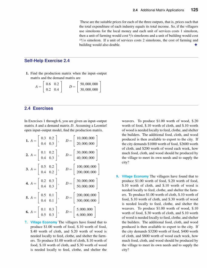
2.4 Additional Matrix Applications 125
These are the suitable prices for each of the three outputs, that is, prices such that
the total expenditure of each industry equals its total income. So, if the villagers
use simoleons for the local money and each unit of services costs 1 simoleon,
then a unit of farming would cost 9/8 simoleons and a unit of building would cost15/16 simoleon. If a unit of services costs 2 simoleons, the cost of farming and
building would also double. ✦
Self-Help Exercise 2.4
1. Find the production matrix when the input–output
matrix and the demand matrix are
A =
[
0.6 0.2
0.2 0.4
]
D =
[
50,000,000
30,000,000
]
2.4 Exercises
In Exercises 1 through 6, you are given an input–output
matrix A and a demand matrix D. Assuming a Leontief
open input–output model, find the production matrix.
1. A =
[
0.3 0.2
0.4 0.3
]
, D =
[
10,000,000
20,000,000
]
2. A =
[
0.1 0.2
0.4 0.3
]
, D =
[
30,000,000
40,000,000
]
3. A =
[
0.5 0.2
0.4 0.2
]
, D =
[
100,000,000
200,000,000
]
4. A =
[
0.2 0.3
0.4 0.3
]
, D =
[
30,000,000
50,000,000
]
5. A =
[
0.5 0.1
0.4 0.1
]
, D =
[
200,000,000
300,000,000
]
6. A =
[
0.1 0.3
0.5 0.3
]
, D =
[
5,000,000
6,000,000
]
7. Village Economy The villagers have found that to
produce $1.00 worth of food, $.10 worth of food,
$.40 worth of cloth, and $.20 worth of wood is
needed locally to feed, clothe, and shelter the farm-
ers. To produce $1.00 worth of cloth, $.10 worth of
food, $.10 worth of cloth, and $.30 worth of wood
is needed locally to feed, clothe, and shelter the
weavers. To produce $1.00 worth of wood, $.20
worth of food, $.10 worth of cloth, and $.10 worth
of wood is needed locally to feed, clothe, and shelter
the builders. The additional food, cloth, and wood
produced is then available to export to the city. If
the city demands $1000 worth of food, $2600 worth
of cloth, and $200 worth of wood each week, how
much food, cloth, and wood should be produced by
the village to meet its own needs and to supply the
city?
8. Village Economy The villagers have found that to
produce $1.00 worth of food, $.20 worth of food,
$.10 worth of cloth, and $.10 worth of wood is
needed locally to feed, clothe, and shelter the farm-
ers. To produce $1.00 worth of cloth, $.10 worth of
food, $.10 worth of cloth, and $.30 worth of wood
is needed locally to feed, clothe, and shelter the
weavers. To produce $1.00 worth of wood, $.10
worth of food, $.30 worth of cloth, and $.10 worth
of wood is needed locally to feed, clothe, and shelter
the builders. The additional food, cloth, and wood
produced is then available to export to the city. If
the city demands $3200 worth of food, $400 worth
of cloth, and $800 worth of wood each week, how
much food, cloth, and wood should be produced by
the village to meet its own needs and to supply the
city?
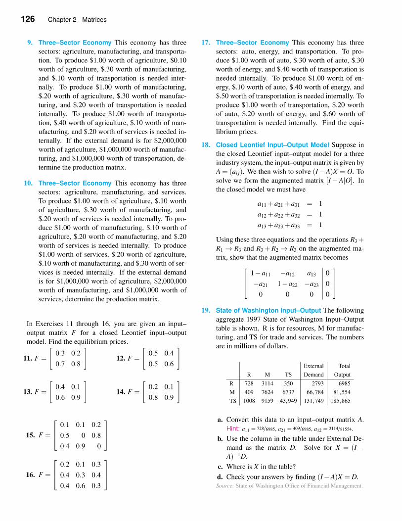
126 Chapter 2 Matrices
9. Three–Sector Economy This economy has three
sectors: agriculture, manufacturing, and transporta-
tion. To produce $1.00 worth of agriculture, $0.10
worth of agriculture, $.30 worth of manufacturing,
and $.10 worth of transportation is needed inter-
nally. To produce $1.00 worth of manufacturing,
$.20 worth of agriculture, $.30 worth of manufac-
turing, and $.20 worth of transportation is needed
internally. To produce $1.00 worth of transporta-
tion, $.40 worth of agriculture, $.10 worth of man-
ufacturing, and $.20 worth of services is needed in-
ternally. If the external demand is for $2,000,000
worth of agriculture, $1,000,000 worth of manufac-
turing, and $1,000,000 worth of transportation, de-
termine the production matrix.
10. Three–Sector Economy This economy has three
sectors: agriculture, manufacturing, and services.
To produce $1.00 worth of agriculture, $.10 worth
of agriculture, $.30 worth of manufacturing, and
$.20 worth of services is needed internally. To pro-
duce $1.00 worth of manufacturing, $.10 worth of
agriculture, $.20 worth of manufacturing, and $.20
worth of services is needed internally. To produce
$1.00 worth of services, $.20 worth of agriculture,
$.10 worth of manufacturing, and $.30 worth of ser-
vices is needed internally. If the external demand
is for $1,000,000 worth of agriculture, $2,000,000
worth of manufacturing, and $1,000,000 worth of
services, determine the production matrix.
In Exercises 11 through 16, you are given an input–
output matrix F for a closed Leontief input–output
model. Find the equilibrium prices.
11. F =
[
0.3 0.2
0.7 0.8
]
12. F =
[
0.5 0.4
0.5 0.6
]
13. F =
[
0.4 0.1
0.6 0.9
]
14. F =
[
0.2 0.1
0.8 0.9
]
15. F =
0.1 0.1 0.2
0.5 0 0.8
0.4 0.9 0
16. F =
0.2 0.1 0.3
0.4 0.3 0.4
0.4 0.6 0.3
17. Three–Sector Economy This economy has three
sectors: auto, energy, and transportation. To pro-
duce $1.00 worth of auto, $.30 worth of auto, $.30
worth of energy, and $.40 worth of transportation is
needed internally. To produce $1.00 worth of en-
ergy, $.10 worth of auto, $.40 worth of energy, and
$.50 worth of transportation is needed internally. To
produce $1.00 worth of transportation, $.20 worth
of auto, $.20 worth of energy, and $.60 worth of
transportation is needed internally. Find the equi-
librium prices.
18. Closed Leontief Input–Output Model Suppose in
the closed Leontief input–output model for a three
industry system, the input–output matrix is given by
A = (ai j). We then wish to solve (I−A)X = O. To
solve we form the augmented matrix [I−A|O]. In
the closed model we must have
a11 +a21 +a31 = 1
a12 +a22 +a32 = 1
a13 +a23 +a33 = 1
Using these three equations and the operations R3+R1 → R3 and R3 +R2→ R3 on the augmented ma-
trix, show that the augmented matrix becomes
1−a11 −a12 a13 0
−a21 1−a22 −a23 0
0 0 0 0
19. State of Washington Input–Output The following
aggregate 1997 State of Washington Input–Output
table is shown. R is for resources, M for manufac-
turing, and TS for trade and services. The numbers
are in millions of dollars.
External Total
R M TS Demand Output
R 728 3114 350 2793 6985
M 409 7624 6737 66,784 81,554
TS 1008 9159 43,949 131,749 185,865
a. Convert this data to an input–output matrix A.
Hint: a11 = 728/6985, a21 = 409/6985, a12 = 3114/81554.
b. Use the column in the table under External De-
mand as the matrix D. Solve for X = (I −A)−1D.
c. Where is X in the table?
d. Check your answers by finding (I−A)X = D.
Source: State of Washington Office of Financial Management.
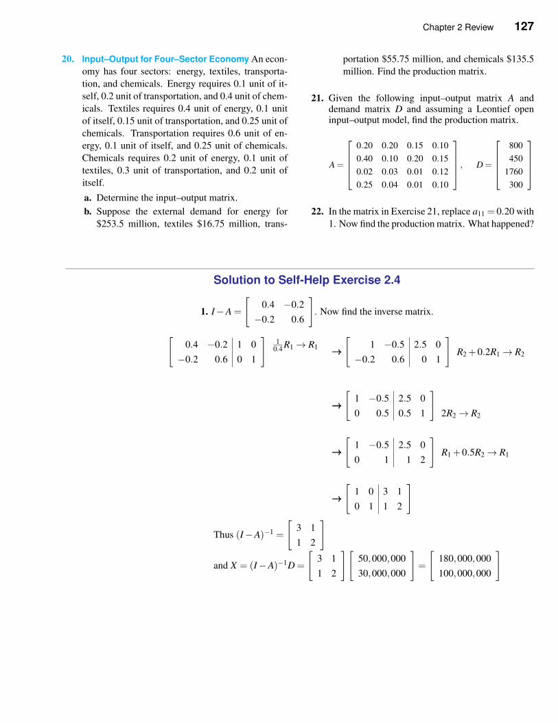
Chapter 2 Review 127
20. Input–Output for Four–Sector Economy An econ-
omy has four sectors: energy, textiles, transporta-
tion, and chemicals. Energy requires 0.1 unit of it-
self, 0.2 unit of transportation, and 0.4 unit of chem-
icals. Textiles requires 0.4 unit of energy, 0.1 unit
of itself, 0.15 unit of transportation, and 0.25 unit of
chemicals. Transportation requires 0.6 unit of en-
ergy, 0.1 unit of itself, and 0.25 unit of chemicals.
Chemicals requires 0.2 unit of energy, 0.1 unit of
textiles, 0.3 unit of transportation, and 0.2 unit of
itself.
a. Determine the input–output matrix.
b. Suppose the external demand for energy for
$253.5 million, textiles $16.75 million, trans-
portation $55.75 million, and chemicals $135.5
million. Find the production matrix.
21. Given the following input–output matrix A anddemand matrix D and assuming a Leontief openinput–output model, find the production matrix.
A =
0.20 0.20 0.15 0.10
0.40 0.10 0.20 0.15
0.02 0.03 0.01 0.12
0.25 0.04 0.01 0.10
, D =
800
450
1760
300
22. In the matrix in Exercise 21, replace a11 = 0.20 with
1. Now find the production matrix. What happened?
Solution to Self-Help Exercise 2.4
1. I−A =
[
0.4 −0.2
−0.2 0.6
]
. Now find the inverse matrix.
[
0.4 −0.2 1 0
−0.2 0.6 0 1
]1
0.4 R1→ R1 →→→[
1 −0.5 2.5 0
−0.2 0.6 0 1
]
R2 +0.2R1→ R2
→→→[
1 −0.5 2.5 0
0 0.5 0.5 1
]
2R2→ R2
→→→[
1 −0.5 2.5 0
0 1 1 2
]
R1 +0.5R2→ R1
→→→[
1 0 3 1
0 1 1 2
]
Thus (I−A)−1 =
[
3 1
1 2
]
and X = (I−A)−1D =
[
3 1
1 2
][
50,000,000
30,000,000
]
=
[
180,000,000
100,000,000
]
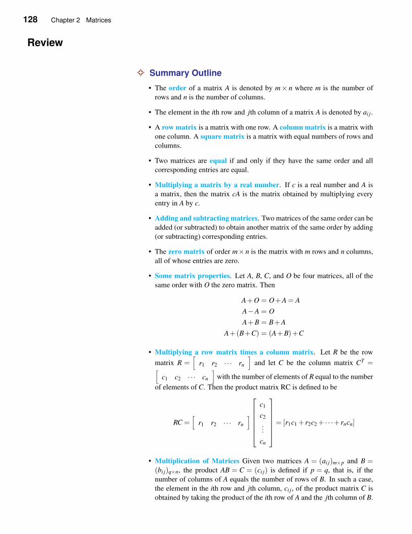
128 Chapter 2 Matrices
Review
✧ Summary Outline
• The order of a matrix A is denoted by m× n where m is the number of
rows and n is the number of columns.
• The element in the ith row and jth column of a matrix A is denoted by ai j.
• A row matrix is a matrix with one row. A column matrix is a matrix with
one column. A square matrix is a matrix with equal numbers of rows and
columns.
• Two matrices are equal if and only if they have the same order and all
corresponding entries are equal.
• Multiplying a matrix by a real number. If c is a real number and A is
a matrix, then the matrix cA is the matrix obtained by multiplying every
entry in A by c.
• Adding and subtracting matrices. Two matrices of the same order can be
added (or subtracted) to obtain another matrix of the same order by adding
(or subtracting) corresponding entries.
• The zero matrix of order m×n is the matrix with m rows and n columns,
all of whose entries are zero.
• Some matrix properties. Let A, B, C, and O be four matrices, all of the
same order with O the zero matrix. Then
A+O = O+A = A
A−A = O
A+B = B+A
A+(B+C) = (A+B)+C
• Multiplying a row matrix times a column matrix. Let R be the row
matrix R =[
r1 r2 · · · rn
]
and let C be the column matrix CT =[
c1 c2 · · · cn
]
with the number of elements of R equal to the number
of elements of C. Then the product matrix RC is defined to be
RC =[
r1 r2 · · · rn
]
c1
c2
...
cn
= [r1c1 + r2c2 + · · ·+ rncn]
• Multiplication of Matrices Given two matrices A = (ai j)m×p and B =(bi j)q×n, the product AB = C = (ci j) is defined if p = q, that is, if the
number of columns of A equals the number of rows of B. In such a case,
the element in the ith row and jth column, ci j, of the product matrix C is
obtained by taking the product of the ith row of A and the jth column of B.
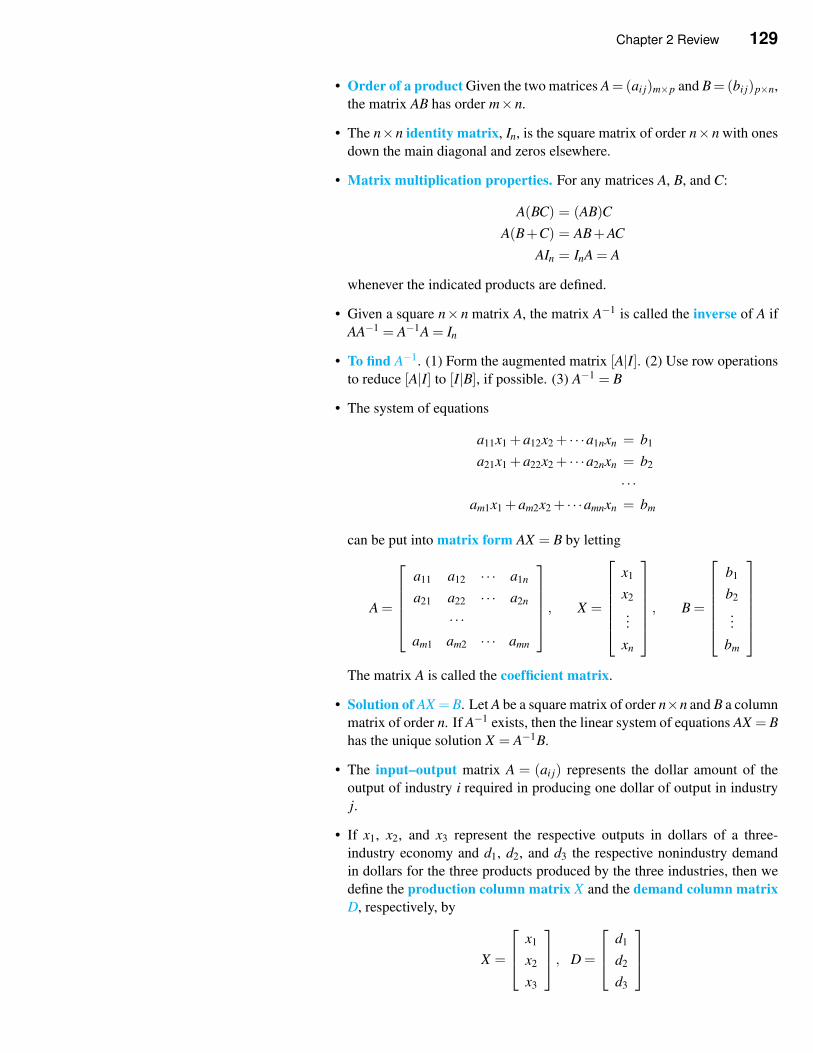
Chapter 2 Review 129
• Order of a product Given the two matrices A=(ai j)m×p and B=(bi j)p×n,
the matrix AB has order m×n.
• The n×n identity matrix, In, is the square matrix of order n×n with ones
down the main diagonal and zeros elsewhere.
• Matrix multiplication properties. For any matrices A, B, and C:
A(BC) = (AB)C
A(B+C) = AB+AC
AIn = InA = A
whenever the indicated products are defined.
• Given a square n×n matrix A, the matrix A−1 is called the inverse of A if
AA−1 = A−1A = In
• To find A−1. (1) Form the augmented matrix [A|I]. (2) Use row operations
to reduce [A|I] to [I|B], if possible. (3) A−1 = B
• The system of equations
a11x1 +a12x2 + · · ·a1nxn = b1
a21x1 +a22x2 + · · ·a2nxn = b2
· · ·am1x1 +am2x2 + · · ·amnxn = bm
can be put into matrix form AX = B by letting
A =
a11 a12 · · · a1n
a21 a22 · · · a2n
· · ·am1 am2 · · · amn
, X =
x1
x2
...
xn
, B =
b1
b2
...
bm
The matrix A is called the coefficient matrix.
• Solution of AX =B. Let A be a square matrix of order n×n and B a column
matrix of order n. If A−1 exists, then the linear system of equations AX = B
has the unique solution X = A−1B.
• The input–output matrix A = (ai j) represents the dollar amount of the
output of industry i required in producing one dollar of output in industry
j.
• If x1, x2, and x3 represent the respective outputs in dollars of a three-
industry economy and d1, d2, and d3 the respective nonindustry demand
in dollars for the three products produced by the three industries, then we
define the production column matrix X and the demand column matrix
D, respectively, by
X =
x1
x2
x3
, D =
d1
d2
d3
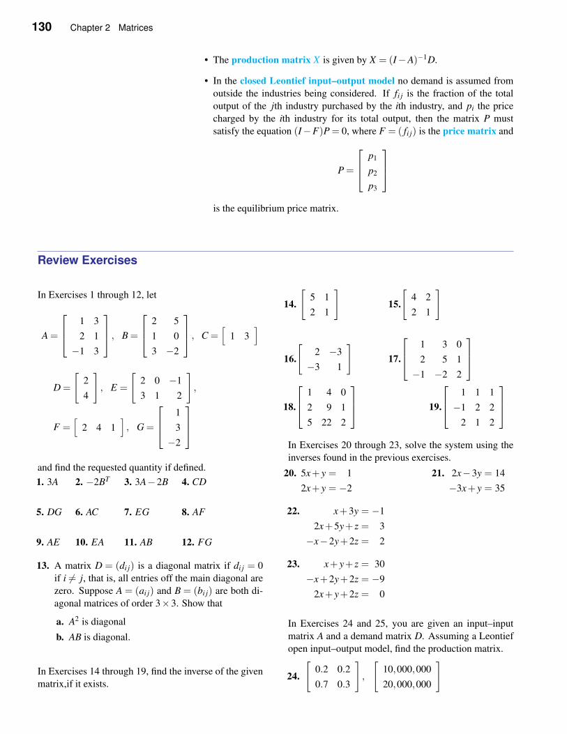
130 Chapter 2 Matrices
• The production matrix X is given by X = (I−A)−1D.
• In the closed Leontief input–output model no demand is assumed from
outside the industries being considered. If fi j is the fraction of the total
output of the jth industry purchased by the ith industry, and pi the price
charged by the ith industry for its total output, then the matrix P must
satisfy the equation (I−F)P = 0, where F = ( fi j) is the price matrix and
P =
p1
p2
p3
is the equilibrium price matrix.
Review Exercises
In Exercises 1 through 12, let
A =
1 3
2 1
−1 3
, B =
2 5
1 0
3 −2
, C =
[
1 3]
D =
[
2
4
]
, E =
[
2 0 −1
3 1 2
]
,
F =[
2 4 1]
, G =
1
3
−2
and find the requested quantity if defined.
1. 3A 2. −2BT 3. 3A−2B 4. CD
5. DG 6. AC 7. EG 8. AF
9. AE 10. EA 11. AB 12. FG
13. A matrix D = (di j) is a diagonal matrix if di j = 0
if i 6= j, that is, all entries off the main diagonal are
zero. Suppose A = (ai j) and B = (bi j) are both di-
agonal matrices of order 3×3. Show that
a. A2 is diagonal
b. AB is diagonal.
In Exercises 14 through 19, find the inverse of the given
matrix,if it exists.
14.
[
5 1
2 1
]
15.
[
4 2
2 1
]
16.
[
2 −3
−3 1
]
17.
1 3 0
2 5 1
−1 −2 2
18.
1 4 0
2 9 1
5 22 2
19.
1 1 1
−1 2 2
2 1 2
In Exercises 20 through 23, solve the system using the
inverses found in the previous exercises.
20. 5x+ y = 1
2x+ y = −2
21. 2x−3y = 14
−3x+ y = 35
22. x+3y = −1
2x+5y+ z = 3
−x−2y+2z = 2
23. x+ y+ z = 30
−x+2y+2z = −9
2x+ y+2z = 0
In Exercises 24 and 25, you are given an input–input
matrix A and a demand matrix D. Assuming a Leontief
open input–output model, find the production matrix.
24.
[
0.2 0.2
0.7 0.3
]
,
[
10,000,000
20,000,000
]
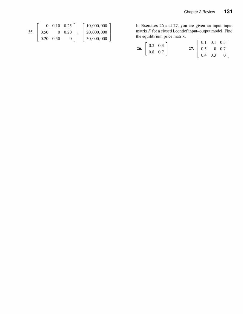
Chapter 2 Review 131
25.
0 0.10 0.25
0.50 0 0.20
0.20 0.30 0
,
10,000,000
20,000,000
30,000,000
In Exercises 26 and 27, you are given an input–input
matrix F for a closed Leontief input–output model. Find
the equilibrium price matrix.
26.
[
0.2 0.3
0.8 0.7
]
27.
0.1 0.1 0.3
0.5 0 0.7
0.4 0.3 0

CHAPTER 3Linear Programming
CONNECTION
Jan de Wit Company
The Jan de Wit company implemented a
decision-support system based on linear
programming as a production-planning and trade
tool for the management of its lily flower business.
The linear programming maximizes the farm’s
total contribution margin, subject to such
constraints as market-defined sales limits, market
requirements, characteristics of the production
cycle duration, technical requirements, bulb
inventory, and greenhouse limitations. The main
decision variable to be calculated is the number of
flower beds in a specific greenhouse, from a
specific bulb patch, of a specific variety, for a
specific purpose, taking into consideration planting
and expected harvesting weeks.
Source: Caixeta-Filho, van Swaay-Neto, and
de Pádua Wagemaker 2002
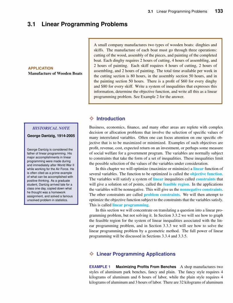
3.1 Linear Programming Problems 133
3.1 Linear Programming Problems
APPLICATION
Manufacture of Wooden Boats
A small company manufactures two types of wooden boats: dinghies and
skiffs. The manufacture of each boat must go through three operations:
cutting of the wood, assembly of the pieces, and painting of the completed
boat. Each dinghy requires 2 hours of cutting, 4 hours of assembling, and
2 hours of painting. Each skiff requires 4 hours of cutting, 2 hours of
assembling, and 2 hours of painting. The total time available per week in
the cutting section is 80 hours, in the assembly section 50 hours, and in
the painting section 50 hours. There is a profit of $60 for every dinghy
and $80 for every skiff. Write a system of inequalities that expresses this
information, determine the objective function, and write all this as a linear
programming problem. See Example 2 for the answer.
✧ Introduction
Business, economics, finance, and many other areas are replete with complex
decision or allocation problems that involve the selection of specific values of
many interrelated variables. Often one can focus attention on one specific ob-
jective that is to be maximized or minimized. Examples of such objectives are
profit, revenue, cost, expected return on an investment, or perhaps some measure
of social welfare for a government program. The variables are normally subject
to constraints that take the form of a set of inequalities. These inequalities limit
the possible selection of the values of the variables under consideration.
HISTORICAL NOTE
George Dantzig, 1914-2005
George Dantzig is considered the
father of linear programming. His
major accomplishments in linear
programming were made during
and immediately after World War II
while working for the Air Force. He
is often cited as a prime example
of what can be accomplished with
positive thinking. As a graduate
student, Dantzig arrived late for a
class one day, copied down what
he thought was a homework
assignment, and solved a famous
unsolved problem in statistics.
In this chapter we will optimize (maximize or minimize) a linear function of
several variables. The function to be optimized is called the objective function.
The variables will satisfy a system of linear inequalities called constraints that
will give a solution set of points, called the feasible region. In the applications
the variables will be nonnegative. This will give us the nonnegative constraints.
The other constraints are called problem constraints. We will then attempt to
optimize the objective function subject to the constraints that the variables satisfy.
This is called linear programming.
In this section we will concentrate on translating a question into a linear pro-
gramming problem, but not solving it. In Section 3.3.2 we will see how to graph
the feasible region for the system of linear inequalities associated with the lin-
ear programming problem, and in Section 3.3.3 we will see how to solve the
linear programming problem by a geometric method. The full power of linear
programming will be discussed in Sections 3.3.4 and 3.3.5.
✧ Linear Programming Applications
EXAMPLE 1 Maximizing Profits From Benches A shop manufactures two
styles of aluminum park benches, fancy and plain. The fancy style requires 4
kilograms of aluminum and 6 hours of labor, while the plain style requires 4
kilograms of aluminum and 3 hours of labor. There are 32 kilograms of aluminum
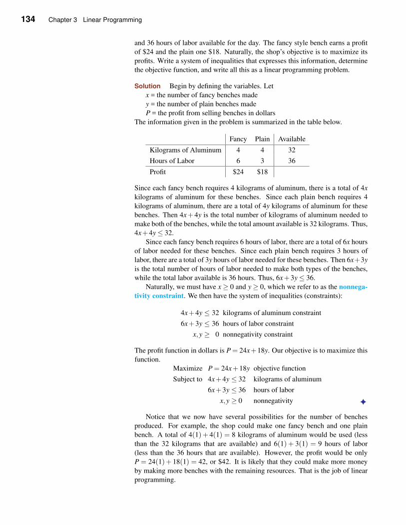
134 Chapter 3 Linear Programming
and 36 hours of labor available for the day. The fancy style bench earns a profit
of $24 and the plain one $18. Naturally, the shop’s objective is to maximize its
profits. Write a system of inequalities that expresses this information, determine
the objective function, and write all this as a linear programming problem.
Solution Begin by defining the variables. Let
x = the number of fancy benches made
y = the number of plain benches made
P = the profit from selling benches in dollars
The information given in the problem is summarized in the table below.
Fancy Plain Available
Kilograms of Aluminum 4 4 32
Hours of Labor 6 3 36
Profit $24 $18
Since each fancy bench requires 4 kilograms of aluminum, there is a total of 4x
kilograms of aluminum for these benches. Since each plain bench requires 4
kilograms of aluminum, there are a total of 4y kilograms of aluminum for these
benches. Then 4x+ 4y is the total number of kilograms of aluminum needed to
make both of the benches, while the total amount available is 32 kilograms. Thus,
4x+4y≤ 32.
Since each fancy bench requires 6 hours of labor, there are a total of 6x hours
of labor needed for these benches. Since each plain bench requires 3 hours of
labor, there are a total of 3y hours of labor needed for these benches. Then 6x+3y
is the total number of hours of labor needed to make both types of the benches,
while the total labor available is 36 hours. Thus, 6x+3y≤ 36.
Naturally, we must have x≥ 0 and y≥ 0, which we refer to as the nonnega-
tivity constraint. We then have the system of inequalities (constraints):
4x+4y ≤ 32 kilograms of aluminum constraint
6x+3y ≤ 36 hours of labor constraint
x,y ≥ 0 nonnegativity constraint
The profit function in dollars is P = 24x+18y. Our objective is to maximize this
function.
Maximize P = 24x+18y objective function
Subject to 4x+4y ≤ 32 kilograms of aluminum
6x+3y ≤ 36 hours of labor
x,y ≥ 0 nonnegativity ✦
Notice that we now have several possibilities for the number of benches
produced. For example, the shop could make one fancy bench and one plain
bench. A total of 4(1)+ 4(1) = 8 kilograms of aluminum would be used (less
than the 32 kilograms that are available) and 6(1) + 3(1) = 9 hours of labor
(less than the 36 hours that are available). However, the profit would be only
P = 24(1)+ 18(1) = 42, or $42. It is likely that they could make more money
by making more benches with the remaining resources. That is the job of linear
programming.
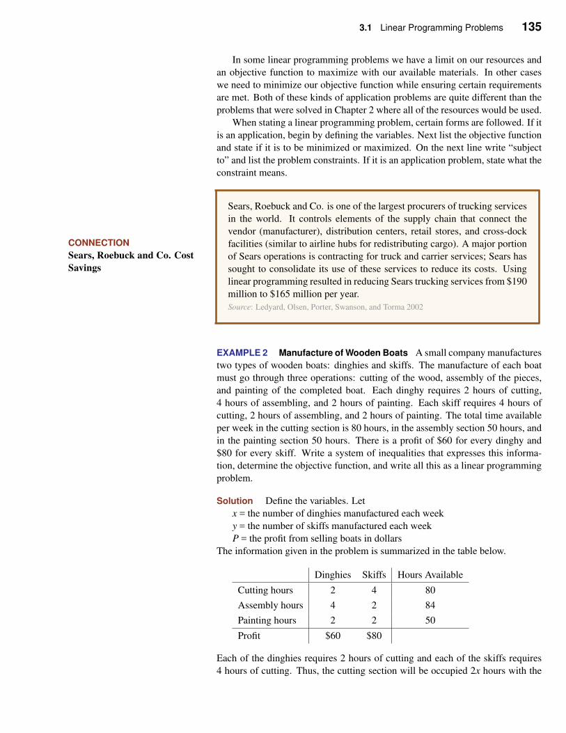
3.1 Linear Programming Problems 135
In some linear programming problems we have a limit on our resources and
an objective function to maximize with our available materials. In other cases
we need to minimize our objective function while ensuring certain requirements
are met. Both of these kinds of application problems are quite different than the
problems that were solved in Chapter 2 where all of the resources would be used.
When stating a linear programming problem, certain forms are followed. If it
is an application, begin by defining the variables. Next list the objective function
and state if it is to be minimized or maximized. On the next line write “subject
to” and list the problem constraints. If it is an application problem, state what the
constraint means.
CONNECTION
Sears, Roebuck and Co. Cost
Savings
Sears, Roebuck and Co. is one of the largest procurers of trucking services
in the world. It controls elements of the supply chain that connect the
vendor (manufacturer), distribution centers, retail stores, and cross-dock
facilities (similar to airline hubs for redistributing cargo). A major portion
of Sears operations is contracting for truck and carrier services; Sears has
sought to consolidate its use of these services to reduce its costs. Using
linear programming resulted in reducing Sears trucking services from $190
million to $165 million per year.
Source: Ledyard, Olsen, Porter, Swanson, and Torma 2002
EXAMPLE 2 Manufacture of Wooden Boats A small company manufactures
two types of wooden boats: dinghies and skiffs. The manufacture of each boat
must go through three operations: cutting of the wood, assembly of the pieces,
and painting of the completed boat. Each dinghy requires 2 hours of cutting,
4 hours of assembling, and 2 hours of painting. Each skiff requires 4 hours of
cutting, 2 hours of assembling, and 2 hours of painting. The total time available
per week in the cutting section is 80 hours, in the assembly section 50 hours, and
in the painting section 50 hours. There is a profit of $60 for every dinghy and
$80 for every skiff. Write a system of inequalities that expresses this informa-
tion, determine the objective function, and write all this as a linear programming
problem.
Solution Define the variables. Let
x = the number of dinghies manufactured each week
y = the number of skiffs manufactured each week
P = the profit from selling boats in dollars
The information given in the problem is summarized in the table below.
Dinghies Skiffs Hours Available
Cutting hours 2 4 80
Assembly hours 4 2 84
Painting hours 2 2 50
Profit $60 $80
Each of the dinghies requires 2 hours of cutting and each of the skiffs requires
4 hours of cutting. Thus, the cutting section will be occupied 2x hours with the
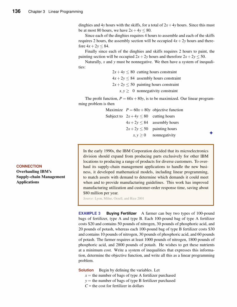
136 Chapter 3 Linear Programming
dinghies and 4y hours with the skiffs, for a total of 2x+4y hours. Since this must
be at most 80 hours, we have 2x+4y≤ 80.
Since each of the dinghies requires 4 hours to assemble and each of the skiffs
requires 2 hours, the assembly section will be occupied 4x+2y hours and there-
fore 4x+2y≤ 84.
Finally since each of the dinghies and skiffs requires 2 hours to paint, the
painting section will be occupied 2x+2y hours and therefore 2x+2y≤ 50.
Naturally, x and y must be nonnegative. We then have a system of inequali-
ties:2x+4y ≤ 80 cutting hours constraint
4x+2y ≤ 84 assembly hours constraint
2x+2y ≤ 50 painting hours constraint
x,y ≥ 0 nonnegativity constraint
The profit function, P = 60x+80y, is to be maximized. Our linear program-
ming problem is then
Maximize P = 60x+80y objective function
Subject to 2x+4y ≤ 80 cutting hours
4x+2y ≤ 84 assembly hours
2x+2y ≤ 50 painting hours
x,y ≥ 0 nonnegativity✦
CONNECTION
Overhauling IBM’s
Supply-chain Management
Applications
In the early 1990s, the IBM Corporation decided that its microelectronics
division should expand from producing parts exclusively for other IBM
locations to producing a range of products for diverse customers. To over-
haul its supply-chain management applications to handle the new busi-
ness, it developed mathematical models, including linear programming,
to match assets with demand to determine which demands it could meet
when and to provide manufacturing guidelines. This work has improved
manufacturing utilization and customer-order response time, saving about
$80 million per year.
Source: Lyon, Milne, Orzell, and Rice 2001
EXAMPLE 3 Buying Fertilizer A farmer can buy two types of 100-pound
bags of fertilizer, type A and type B. Each 100-pound bag of type A fertilizer
costs $20 and contains 50 pounds of nitrogen, 30 pounds of phosphoric acid, and
20 pounds of potash, whereas each 100-pound bag of type B fertilizer costs $30
and contains 10 pounds of nitrogen, 30 pounds of phosphoric acid, and 60 pounds
of potash. The farmer requires at least 1000 pounds of nitrogen, 1800 pounds of
phosphoric acid, and 2800 pounds of potash. He wishes to get these nutrients
at a minimum cost. Write a system of inequalities that expresses this informa-
tion, determine the objective function, and write all this as a linear programming
problem.
Solution Begin by defining the variables. Let
x = the number of bags of type A fertilizer purchased
y = the number of bags of type B fertilizer purchased
C = the cost for fertilizer in dollars
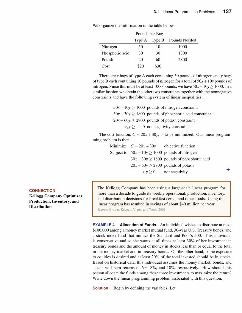
3.1 Linear Programming Problems 137
We organize the information in the table below.
Pounds per Bag
Type A Type B Pounds Needed
Nitrogen 50 10 1000
Phosphoric acid 30 30 1800
Potash 20 60 2800
Cost $20 $30
There are x bags of type A each containing 50 pounds of nitrogen and y bags
of type B each containing 10 pounds of nitrogen for a total of 50x+10y pounds of
nitrogen. Since this must be at least 1000 pounds, we have 50x+10y≥ 1000. In a
similar fashion we obtain the other two constraints together with the nonnegative
constraints and have the following system of linear inequalities:
50x+10y ≥ 1000 pounds of nitrogen constraint
30x+30y ≥ 1800 pounds of phosphoric acid constraint
20x+60y ≥ 2800 pounds of potash constraint
x,y ≥ 0 nonnegativity constraint
The cost function, C = 20x+ 30y, is to be minimized. Our linear program-
ming problem is then
Minimize C = 20x+30y objective function
Subject to 50x+10y ≥ 1000 pounds of nitrogen
30x+30y ≥ 1800 pounds of phosphoric acid
20x+60y ≥ 2800 pounds of potash
x,y ≥ 0 nonnegativity✦
CONNECTION
Kellogg Company Optimizes
Production, Inventory, and
Distribution
The Kellogg Company has been using a large-scale linear program for
more than a decade to guide its weekly operational, production, inventory,
and distribution decisions for breakfast cereal and other foods. Using this
linear program has resulted in savings of about $40 million per year.
Source: Brown, Keegan, Vigus, and Wood 2001
EXAMPLE 4 Allocation of Funds An individual wishes to distribute at most
$100,000 among a money market mutual fund, 30-year U.S. Treasury bonds, and
a stock index fund that mimics the Standard and Poor’s 500. This individual
is conservative and so she wants at all times at least 30% of her investment in
treasury bonds and the amount of money in stocks less than or equal to the total
in the money market and in treasury bonds. On the other hand, some exposure
to equities is desired and at least 20% of the total invested should be in stocks.
Based on historical data, this individual assumes the money market, bonds, and
stocks will earn returns of 6%, 8%, and 10%, respectively. How should this
person allocate the funds among these three investments to maximize the return?
Write down the linear programming problem associated with this question.
Solution Begin by defining the variables. Let
138 Chapter 3 Linear Programming
x = the amount in thousands of dollars invested in the money market
y = the amount in thousands of dollars invested in bonds
z = the amount in thousands of dollars invested in stocks
R = the amount of returns in thousands of dollars
Since the total must be at most $100,000, x+ y+ z≤ 100. At least 30% must be
in bonds and so we have y ≥ 0.30(x+ y+ z) and since at least 20% must be in
stocks, z≥ 0.20(x+ y+ z). We also have the amount in stocks less than or equal
to the totals in the money market and bonds. Thus, z ≤ x+ y. We then have the
following system of inequalities or constraints.
x+ y+ z ≤ 100 total money in thousands of dollars
z ≤ x+ y ratio of money market and bonds to stocks
y ≥ 0.3(x+ y+ z) minimum invested in bonds
z ≥ 0.2(x+ y+ z) minimum invested in stocks
x,y,z ≥ 0 nonnegativity constraint
We always prefer to have all variables on the left of the inequalities. The first
inequality is already in that form. The second inequality is rewritten as
z ≤ x+ y subtract x and y from both sides
−x− y+ z ≤ 0
The third inequality as
y ≥ 0.3(x+ y+ z) multiply out and rearrange
0.3x+0.3y+0.3z ≤ y subtract y from both sides
0.3x−0.7y+0.3z ≤ 0
The fourth inequality as
z ≥ 0.2(x+ y+ z) multiply out and rearrange
0.2x+0.2y−0.8z ≤ 0
The objective function is the return in dollars, R = 60x+ 80y+ 100z, since we
defined our variables in thousands of dollars. The linear programming problem
is then
Maximize R = 60x+80y+100z objective function
Subject to x+ y+ z ≤ 100 available funds
−x− y+ z ≤ 0 ratio
0.3x−0.7y+0.3z ≤ 0 minimum invested in bonds
0.2x+0.2y−0.8z ≤ 0 minimum invested in stocks
x,y,z ≥ 0 nonnegativity✦
EXAMPLE 5 Transportation of Flat Screen Monitors A firm has two stock-
piles of large flat screen monitors in warehouses at two different locations, Den-
ver (D) and Santa Fe (SF). The monitors must be shipped to two plants, located in
Des Moines (DM) and Fort Wayne (FW) , for assembly into home entertainment
centers. At the beginning of a week the stockpile at Denver has 150 flat screens
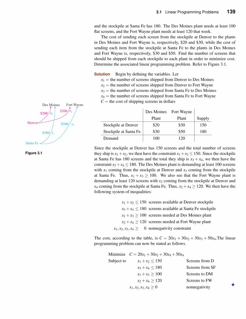
3.1 Linear Programming Problems 139
and the stockpile at Santa Fe has 180. The Des Moines plant needs at least 100
flat screens, and the Fort Wayne plant needs at least 120 that week.
The cost of sending each screen from the stockpile at Denver to the plants
in Des Moines and Fort Wayne is, respectively, $20 and $30, while the cost of
sending each item from the stockpile at Santa Fe to the plants in Des Moines
and Fort Wayne is, respectively, $30 and $50. Find the number of screens that
should be shipped from each stockpile to each plant in order to minimize cost.
Determine the associated linear programming problem. Refer to Figure 3.1.
Solution Begin by defining the variables. Let
x1 = the number of screens shipped from Denver to Des Moines
x2 = the number of screens shipped from Denver to Fort Wayne
x3 = the number of screens shipped from Santa Fe to Des Moines
x4 = the number of screens shipped from Santa Fe to Fort Wayne
C = the cost of shipping screens in dollars
Figure 3.1
Des Moines Fort Wayne
Plant Plant Supply
Stockpile at Denver $20 $30 150
Stockpile at Santa Fe $30 $50 180
Demand 100 120
Since the stockpile at Denver has 150 screens and the total number of screens
they ship is x1+x2, we then have the constraint x1+x2≤ 150. Since the stockpile
at Santa Fe has 180 screens and the total they ship is x3 + x4, we then have the
constraint x3+x4≤ 180. The Des Moines plant is demanding at least 100 screens
with x1 coming from the stockpile at Denver and x3 coming from the stockpile
at Santa Fe. Thus, x1 + x3 ≥ 100. We also see that the Fort Wayne plant is
demanding at least 120 screens with x2 coming from the stockpile at Denver and
x4 coming from the stockpile at Santa Fe. Thus, x2 +x4 ≥ 120. We then have the
following system of inequalities:
x1 + x2 ≤ 150 screens available at Denver stockpile
x3 + x4 ≤ 180 screens available at Santa Fe stockpile
x1 + x3 ≥ 100 screens needed at Des Moines plant
x2 + x4 ≥ 120 screens needed at Fort Wayne plant
x1,x2,x3,x4 ≥ 0 nonnegativity constraint
The cost, according to the table, is C = 20x1 + 30x2 + 30x3 + 50x4.The linear
programming problem can now be stated as follows.
Minimize C = 20x1 +30x2 +30x4 +50x4
Subject to x1 + x2 ≤ 150 Screens from D
x3 + x4 ≤ 180 Screens from SF
x1 + x3 ≥ 100 Screens to DM
x2 + x4 ≥ 120 Screens to FW
x1,x2,x3,x4 ≥ 0 nonnegativity✦
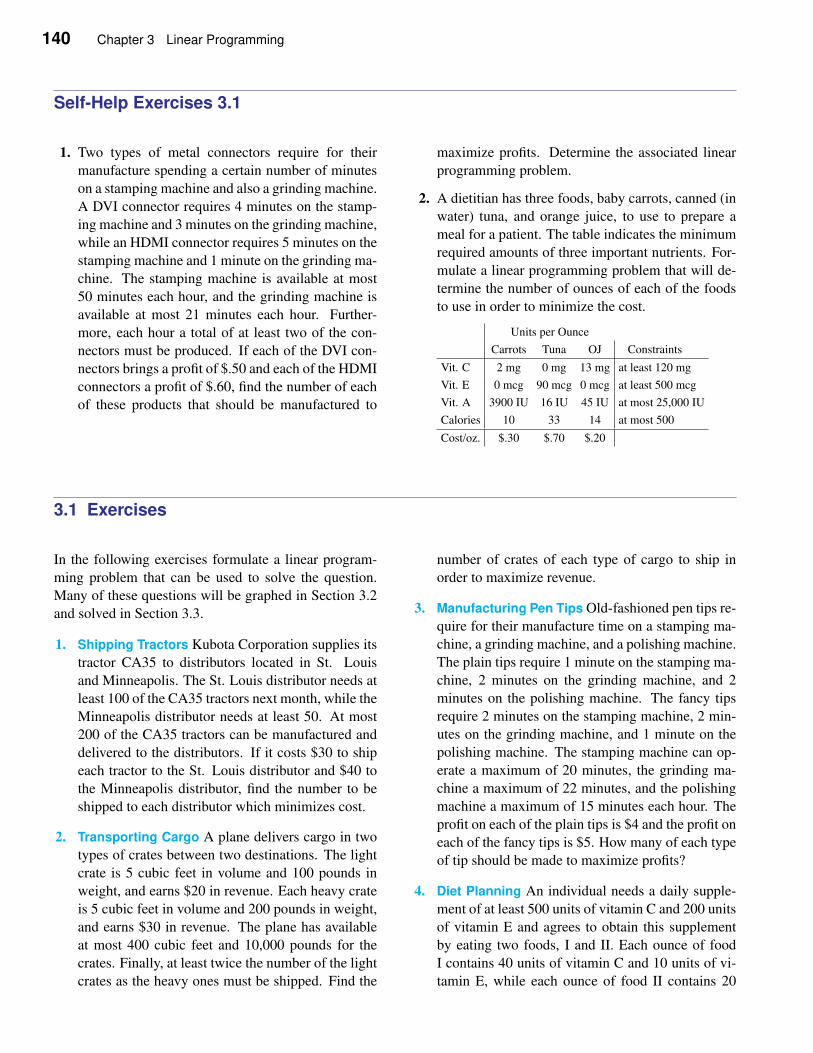
140 Chapter 3 Linear Programming
Self-Help Exercises 3.1
1. Two types of metal connectors require for their
manufacture spending a certain number of minutes
on a stamping machine and also a grinding machine.
A DVI connector requires 4 minutes on the stamp-
ing machine and 3 minutes on the grinding machine,
while an HDMI connector requires 5 minutes on the
stamping machine and 1 minute on the grinding ma-
chine. The stamping machine is available at most
50 minutes each hour, and the grinding machine is
available at most 21 minutes each hour. Further-
more, each hour a total of at least two of the con-
nectors must be produced. If each of the DVI con-
nectors brings a profit of $.50 and each of the HDMI
connectors a profit of $.60, find the number of each
of these products that should be manufactured to
maximize profits. Determine the associated linear
programming problem.
2. A dietitian has three foods, baby carrots, canned (in
water) tuna, and orange juice, to use to prepare a
meal for a patient. The table indicates the minimum
required amounts of three important nutrients. For-
mulate a linear programming problem that will de-
termine the number of ounces of each of the foods
to use in order to minimize the cost.
Units per Ounce
Carrots Tuna OJ Constraints
Vit. C 2 mg 0 mg 13 mg at least 120 mg
Vit. E 0 mcg 90 mcg 0 mcg at least 500 mcg
Vit. A 3900 IU 16 IU 45 IU at most 25,000 IU
Calories 10 33 14 at most 500
Cost/oz. $.30 $.70 $.20
3.1 Exercises
In the following exercises formulate a linear program-
ming problem that can be used to solve the question.
Many of these questions will be graphed in Section 3.2
and solved in Section 3.3.
1. Shipping Tractors Kubota Corporation supplies its
tractor CA35 to distributors located in St. Louis
and Minneapolis. The St. Louis distributor needs at
least 100 of the CA35 tractors next month, while the
Minneapolis distributor needs at least 50. At most
200 of the CA35 tractors can be manufactured and
delivered to the distributors. If it costs $30 to ship
each tractor to the St. Louis distributor and $40 to
the Minneapolis distributor, find the number to be
shipped to each distributor which minimizes cost.
2. Transporting Cargo A plane delivers cargo in two
types of crates between two destinations. The light
crate is 5 cubic feet in volume and 100 pounds in
weight, and earns $20 in revenue. Each heavy crate
is 5 cubic feet in volume and 200 pounds in weight,
and earns $30 in revenue. The plane has available
at most 400 cubic feet and 10,000 pounds for the
crates. Finally, at least twice the number of the light
crates as the heavy ones must be shipped. Find the
number of crates of each type of cargo to ship in
order to maximize revenue.
3. Manufacturing Pen Tips Old-fashioned pen tips re-
quire for their manufacture time on a stamping ma-
chine, a grinding machine, and a polishing machine.
The plain tips require 1 minute on the stamping ma-
chine, 2 minutes on the grinding machine, and 2
minutes on the polishing machine. The fancy tips
require 2 minutes on the stamping machine, 2 min-
utes on the grinding machine, and 1 minute on the
polishing machine. The stamping machine can op-
erate a maximum of 20 minutes, the grinding ma-
chine a maximum of 22 minutes, and the polishing
machine a maximum of 15 minutes each hour. The
profit on each of the plain tips is $4 and the profit on
each of the fancy tips is $5. How many of each type
of tip should be made to maximize profits?
4. Diet Planning An individual needs a daily supple-
ment of at least 500 units of vitamin C and 200 units
of vitamin E and agrees to obtain this supplement
by eating two foods, I and II. Each ounce of food
I contains 40 units of vitamin C and 10 units of vi-
tamin E, while each ounce of food II contains 20
3.1 Linear Programming Problems 141
units of vitamin C and also 20 units of vitamin E.
The total supplement of these two foods must be at
most 30 ounces. Unfortunately, food I contains 30
units of cholesterol per ounce, and food II contains
20 units of cholesterol per ounce. Find the appro-
priate amounts of the two food supplements so that
cholesterol is minimized.
5. Manufacturing Furniture A firm manufactures ta-
bles and desks. To produce each table requires 1
hour of labor, 10 square feet of wood, and 2 quarts
of finish. To produce each desk requires 3 hours of
labor, 20 square feet of wood, and 1 quart of finish.
Available are at most 45 hours of labor, at most 350
square feet of wood, and at most 55 quarts of finish.
The tables and desks yield profits of $4 and $3 re-
spectively. Find the number of each product to be
made in order to maximize profits.
6. Mixed Nuts A dealer has 7600 pounds of peanuts,
5800 pounds of almonds, and 3000 pounds of
cashews to be used to make two mixtures. The first
mixture wholesales for $2 per pound and consists of
60% peanuts, 30% almonds, and 10% cashews. The
second mixture wholesales for $3 per pound and
consists of 20% peanuts, 50% almonds, and 30%
cashews. How many pounds of each mixture should
the dealer make in order to maximize revenue?
7. Fish Food A certain lake has smallmouth and large-
mouth bass and also three types of food for these
fish: minnows, insects, and worms. Each month
the lake can supply 800 pounds of minnows, 500
pounds of insects, and 700 pounds of worms. Each
month each smallmouth bass requires 1 pound of
minnows, 1 pound of insects, and 2 pounds of
worms, and each largemouth bass requires 4 pounds
of minnows, 2 pounds of insects, and 1 pound of
worms. What is the maximum number of these fish
that the lake can support?
8. Scheduling Hot Tubs A firm has plants in Boston
and Baltimore that manufacture three models of
hot tubs: regular, fancy, and super. In one day
the Boston plant can manufacture 30 of the regular
model, 30 of the fancy model, and 10 of the super
model, and costs $3000 a day to operate, whereas
the Baltimore plant can manufacture 10 of the regu-
lar model, 20 of the fancy model, and 30 of the super
model, and costs $4000 a day to operate. At least
240 of the regular model, 390 of the fancy model,
and 410 of the super model are needed. How many
days must each plant operate in order to minimize
cost?
9. Planting Corn Farmer Blue has 100 acres available
to plant white and yellow corn. Each acre of white
corn will yield 95 bushels of corn and each acre
of yellow corn will yield 120 bushels of corn. He
wants to have at least three times as many bushels
of white corn as he does of yellow corn. The white
corn will sell for $4.00 per bushel and the yellow
corn will sell for $3.50 per bushel. How many acres
of each type of corn should Farmer Blue plant to
maximize his revenue?
10. Planting Carrots Farmer Green has 10 acres avail-
able to plant maroon and orange carrots. Each acre
of maroon carrots will yield 2 tons of carrots and
each acre of orange carrots will yield 4 tons of car-
rots. He wants to have at least three times as many
tons of maroon carrots as he does of orange carrots.
The profit for maroon carrots is $200 per ton and the
profit for orange carrots is $100 per ton. How many
acres of each type of carrots should Farmer Green
plant to maximize his profit?
11. Baking Cookies A baker has 50 pounds of oatmeal
to make oatmeal cookies and oatmeal bars. Oatmeal
cookies sell for $1.00 each and oatmeal bars sell for
$1.50 each. A batch of 36 oatmeal cookies requires
2 pounds of oatmeal and a batch of 24 oatmeal bars
requires 1.5 pounds of oatmeal. Additionally she
wants to have twice as many cookies as bars. How
many of each item should she make to maximize
revenue?
12. Fried Treats A baker has 23 pounds of sugar to
make donuts and fritters. Donuts sell for $.50 each
and fritters sell for $1.50 each. A batch of 24 donuts
requires 1.5 pounds of sugar and a batch of 15 frit-
ters requires 2 pounds of sugar. The baker wants
to have four times as many donuts as fritters. How
many of each item should the baker make to maxi-
mize revenue?
13. Investments An individual has at most $100,000 to
invest in four funds: a money market fund, a bond
fund, a conservative stock fund, and a speculative
stock fund. These four investments are assumed to
have annual returns of 6%, 8%, 10%, and 13%, re-
spectively. The investor wants at least $10,000 in
the conservative stock fund, at least $10,000 and
at most $40,000 in the money market fund, the
amount in speculative stocks less than or equal to
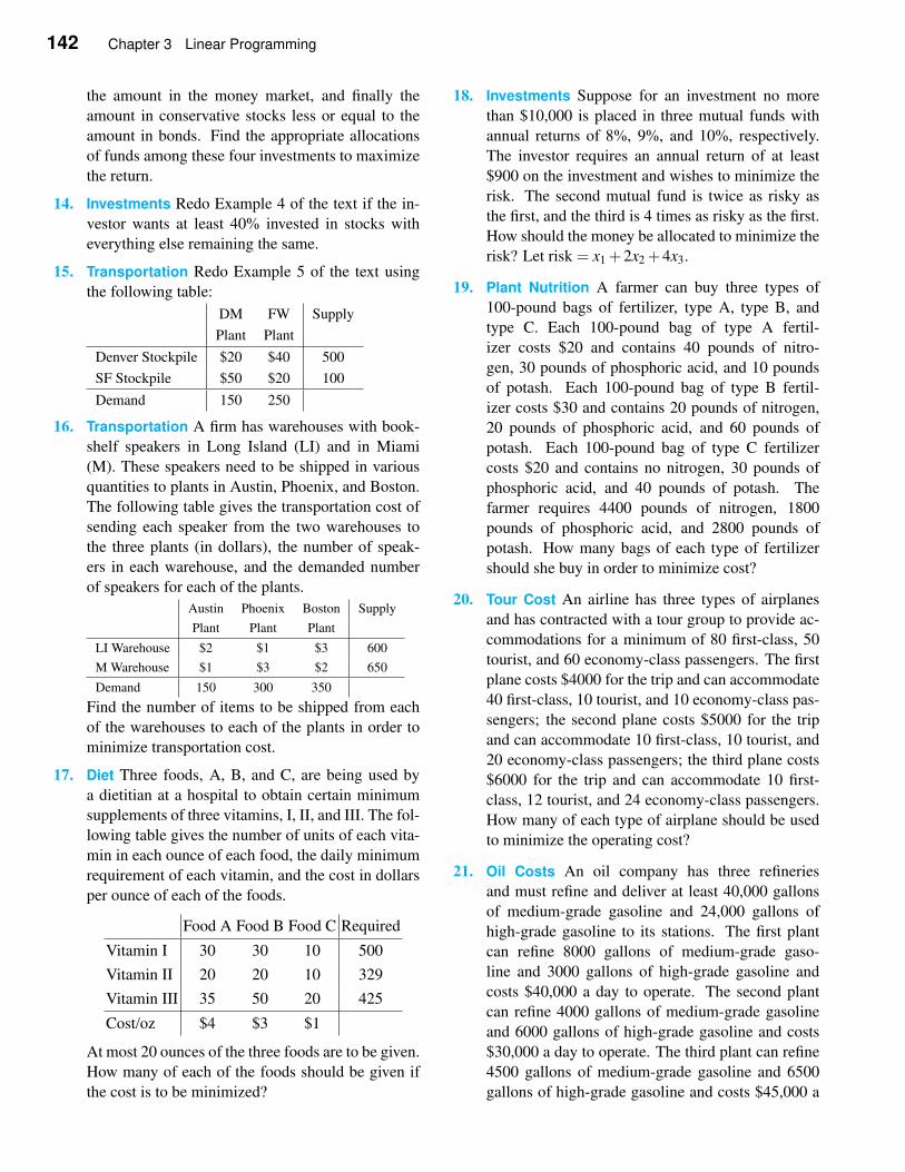
142 Chapter 3 Linear Programming
the amount in the money market, and finally the
amount in conservative stocks less or equal to the
amount in bonds. Find the appropriate allocations
of funds among these four investments to maximize
the return.
14. Investments Redo Example 4 of the text if the in-
vestor wants at least 40% invested in stocks with
everything else remaining the same.
15. Transportation Redo Example 5 of the text using
the following table:
DM FW Supply
Plant Plant
Denver Stockpile $20 $40 500
SF Stockpile $50 $20 100
Demand 150 250
16. Transportation A firm has warehouses with book-
shelf speakers in Long Island (LI) and in Miami
(M). These speakers need to be shipped in various
quantities to plants in Austin, Phoenix, and Boston.
The following table gives the transportation cost of
sending each speaker from the two warehouses to
the three plants (in dollars), the number of speak-
ers in each warehouse, and the demanded number
of speakers for each of the plants.
Austin Phoenix Boston Supply
Plant Plant Plant
LI Warehouse $2 $1 $3 600
M Warehouse $1 $3 $2 650
Demand 150 300 350
Find the number of items to be shipped from each
of the warehouses to each of the plants in order to
minimize transportation cost.
17. Diet Three foods, A, B, and C, are being used by
a dietitian at a hospital to obtain certain minimum
supplements of three vitamins, I, II, and III. The fol-
lowing table gives the number of units of each vita-
min in each ounce of each food, the daily minimum
requirement of each vitamin, and the cost in dollars
per ounce of each of the foods.
Food A Food B Food C Required
Vitamin I 30 30 10 500
Vitamin II 20 20 10 329
Vitamin III 35 50 20 425
Cost/oz $4 $3 $1
At most 20 ounces of the three foods are to be given.
How many of each of the foods should be given if
the cost is to be minimized?
18. Investments Suppose for an investment no more
than $10,000 is placed in three mutual funds with
annual returns of 8%, 9%, and 10%, respectively.
The investor requires an annual return of at least
$900 on the investment and wishes to minimize the
risk. The second mutual fund is twice as risky as
the first, and the third is 4 times as risky as the first.
How should the money be allocated to minimize the
risk? Let risk = x1 +2x2 +4x3.
19. Plant Nutrition A farmer can buy three types of
100-pound bags of fertilizer, type A, type B, and
type C. Each 100-pound bag of type A fertil-
izer costs $20 and contains 40 pounds of nitro-
gen, 30 pounds of phosphoric acid, and 10 pounds
of potash. Each 100-pound bag of type B fertil-
izer costs $30 and contains 20 pounds of nitrogen,
20 pounds of phosphoric acid, and 60 pounds of
potash. Each 100-pound bag of type C fertilizer
costs $20 and contains no nitrogen, 30 pounds of
phosphoric acid, and 40 pounds of potash. The
farmer requires 4400 pounds of nitrogen, 1800
pounds of phosphoric acid, and 2800 pounds of
potash. How many bags of each type of fertilizer
should she buy in order to minimize cost?
20. Tour Cost An airline has three types of airplanes
and has contracted with a tour group to provide ac-
commodations for a minimum of 80 first-class, 50
tourist, and 60 economy-class passengers. The first
plane costs $4000 for the trip and can accommodate
40 first-class, 10 tourist, and 10 economy-class pas-
sengers; the second plane costs $5000 for the trip
and can accommodate 10 first-class, 10 tourist, and
20 economy-class passengers; the third plane costs
$6000 for the trip and can accommodate 10 first-
class, 12 tourist, and 24 economy-class passengers.
How many of each type of airplane should be used
to minimize the operating cost?
21. Oil Costs An oil company has three refineries
and must refine and deliver at least 40,000 gallons
of medium-grade gasoline and 24,000 gallons of
high-grade gasoline to its stations. The first plant
can refine 8000 gallons of medium-grade gaso-
line and 3000 gallons of high-grade gasoline and
costs $40,000 a day to operate. The second plant
can refine 4000 gallons of medium-grade gasoline
and 6000 gallons of high-grade gasoline and costs
$30,000 a day to operate. The third plant can refine
4500 gallons of medium-grade gasoline and 6500
gallons of high-grade gasoline and costs $45,000 a
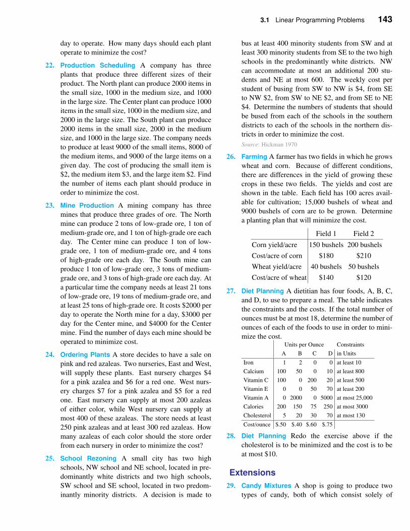
3.1 Linear Programming Problems 143
day to operate. How many days should each plant
operate to minimize the cost?
22. Production Scheduling A company has three
plants that produce three different sizes of their
product. The North plant can produce 2000 items in
the small size, 1000 in the medium size, and 1000
in the large size. The Center plant can produce 1000
items in the small size, 1000 in the medium size, and
2000 in the large size. The South plant can produce
2000 items in the small size, 2000 in the medium
size, and 1000 in the large size. The company needs
to produce at least 9000 of the small items, 8000 of
the medium items, and 9000 of the large items on a
given day. The cost of producing the small item is
$2, the medium item $3, and the large item $2. Find
the number of items each plant should produce in
order to minimize the cost.
23. Mine Production A mining company has three
mines that produce three grades of ore. The North
mine can produce 2 tons of low-grade ore, 1 ton of
medium-grade ore, and 1 ton of high-grade ore each
day. The Center mine can produce 1 ton of low-
grade ore, 1 ton of medium-grade ore, and 4 tons
of high-grade ore each day. The South mine can
produce 1 ton of low-grade ore, 3 tons of medium-
grade ore, and 3 tons of high-grade ore each day. At
a particular time the company needs at least 21 tons
of low-grade ore, 19 tons of medium-grade ore, and
at least 25 tons of high-grade ore. It costs $2000 per
day to operate the North mine for a day, $3000 per
day for the Center mine, and $4000 for the Center
mine. Find the number of days each mine should be
operated to minimize cost.
24. Ordering Plants A store decides to have a sale on
pink and red azaleas. Two nurseries, East and West,
will supply these plants. East nursery charges $4
for a pink azalea and $6 for a red one. West nurs-
ery charges $7 for a pink azalea and $5 for a red
one. East nursery can supply at most 200 azaleas
of either color, while West nursery can supply at
most 400 of these azaleas. The store needs at least
250 pink azaleas and at least 300 red azaleas. How
many azaleas of each color should the store order
from each nursery in order to minimize the cost?
25. School Rezoning A small city has two high
schools, NW school and NE school, located in pre-
dominantly white districts and two high schools,
SW school and SE school, located in two predom-
inantly minority districts. A decision is made to
bus at least 400 minority students from SW and at
least 300 minority students from SE to the two high
schools in the predominantly white districts. NW
can accommodate at most an additional 200 stu-
dents and NE at most 600. The weekly cost per
student of busing from SW to NW is $4, from SE
to NW $2, from SW to NE $2, and from SE to NE
$4. Determine the numbers of students that should
be bused from each of the schools in the southern
districts to each of the schools in the northern dis-
tricts in order to minimize the cost.
Source: Hickman 1970
26. Farming A farmer has two fields in which he grows
wheat and corn. Because of different conditions,
there are differences in the yield of growing these
crops in these two fields. The yields and cost are
shown in the table. Each field has 100 acres avail-
able for cultivation; 15,000 bushels of wheat and
9000 bushels of corn are to be grown. Determine
a planting plan that will minimize the cost.
Field 1 Field 2
Corn yield/acre 150 bushels 200 bushels
Cost/acre of corn $180 $210
Wheat yield/acre 40 bushels 50 bushels
Cost/acre of wheat $140 $120
27. Diet Planning A dietitian has four foods, A, B, C,
and D, to use to prepare a meal. The table indicates
the constraints and the costs. If the total number of
ounces must be at most 18, determine the number of
ounces of each of the foods to use in order to mini-
mize the cost.Units per Ounce Constraints
A B C D in Units
Iron 1 2 0 0 at least 10
Calcium 100 50 0 10 at least 800
Vitamin C 100 0 200 20 at least 500
Vitamin E 0 0 50 70 at least 200
Vitamin A 0 2000 0 5000 at most 25,000
Calories 200 150 75 250 at most 3000
Cholesterol 5 20 30 70 at most 130
Cost/ounce $.50 $.40 $.60 $.75
28. Diet Planning Redo the exercise above if the
cholesterol is to be minimized and the cost is to be
at most $10.
Extensions
29. Candy Mixtures A shop is going to produce two
types of candy, both of which consist solely of
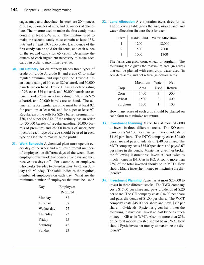
144 Chapter 3 Linear Programming
sugar, nuts, and chocolate. In stock are 200 ounces
of sugar, 30 ounces of nuts, and 60 ounces of choco-
late. The mixture used to make the first candy must
contain at least 25% nuts. The mixture used to
make the second candy must contain at least 15%
nuts and at least 10% chocolate. Each ounce of the
first candy can be sold for 50 cents, and each ounce
of the second candy for 65 cents. Determine the
ounces of each ingredient necessary to make each
candy in order to maximize revenue.
30. Oil Refinery An oil refinery blends three types of
crude oil, crude A, crude B, and crude C, to make
regular, premium, and super gasoline. Crude A has
an octane rating of 90, costs $20 a barrel, and 50,000
barrels are on hand. Crude B has an octane rating
of 96, costs $24 a barrel, and 30,000 barrels are on
hand. Crude C has an octane rating of 98, costs $26
a barrel, and 20,000 barrels are on hand. The oc-
tane rating for regular gasoline must be at least 92,
for premium at least 96, and for super at least 97.
Regular gasoline sells for $26 a barrel, premium for
$30, and super for $32. If the refinery has an order
for 30,000 barrels of regular gasoline, 20,000 bar-
rels of premium, and 28,000 barrels of super, how
much of each type of crude should be used in each
type of gasoline to maximize the profit?
31. Work Schedule A chemical plant must operate ev-
ery day of the week and requires different numbers
of employees on different days of the week. Each
employee must work five consecutive days and then
receive two days off. For example, an employee
who works Tuesday to Saturday must be off on Sun-
day and Monday. The table indicates the required
number of employees on each day. What are the
minimum number of employees that must be used?
Day Employees
Required
Monday 82
Tuesday 87
Wednesday 77
Thursday 73
Friday 75
Saturday 42
Sunday 23
32. Land Allocation A corporation owns three farms.
The following table gives the size, usable land, and
water allocation (in acre-feet) for each:
Farm Usable Land Water Allocation
1 1200 18,000
2 1500 2000
3 1000 1300
The farms can grow corn, wheat, or sorghum. The
following table gives the maximum area (in acres)
that can be planted with each crop, water used (in
acre-feet/acre), and net return (in dollars/acre):
Maximum Water Net
Crop Area Used Return
Corn 1400 3 500
Wheat 1500 2 400
Sorghum 1700 1 100
How many acres of each crop should be planted on
each farm to maximize net return.
33. Investment Planning Mazie has at most $12,000
to invest in three different stocks. The KO com-
pany costs $42.00 per share and pays dividends of
$1.25 per share. The INTC company costs $21.00
per share and pays dividends of $.40 per share. The
MCD company costs $35.00 per share and pays $.67
per share in dividends. Mazie has given her broker
the following instructions: Invest at least twice as
much money in INTC as in KO. Also, no more than
25% of the total invested should be in MCD. How
should Mazie invest her money to maximize the div-
idends?
34. Investment Planning Pyxie has at most $20,000 to
invest in three different stocks. The TWX company
costs $17.00 per share and pays dividends of $.20
per share. The GE company costs $34.00 per share
and pays dividends of $1.00 per share. The WMT
company costs $45.00 per share and pays $.67 per
share in dividends. Pyxie has given her broker the
following instructions: Invest at least twice as much
money in GE as in WMT. Also, no more than 25%
of the total money invested should be in TWX. How
should Pyxie invest her money to maximize the div-
idends?
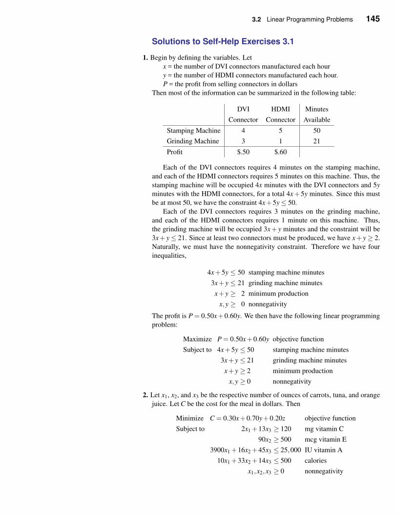
3.2 Linear Programming Problems 145
Solutions to Self-Help Exercises 3.1
1. Begin by defining the variables. Let
x = the number of DVI connectors manufactured each hour
y = the number of HDMI connectors manufactured each hour.
P = the profit from selling connectors in dollars
Then most of the information can be summarized in the following table:
DVI HDMI Minutes
Connector Connector Available
Stamping Machine 4 5 50
Grinding Machine 3 1 21
Profit $.50 $.60
Each of the DVI connectors requires 4 minutes on the stamping machine,
and each of the HDMI connectors requires 5 minutes on this machine. Thus, the
stamping machine will be occupied 4x minutes with the DVI connectors and 5y
minutes with the HDMI connectors, for a total 4x+5y minutes. Since this must
be at most 50, we have the constraint 4x+5y≤ 50.
Each of the DVI connectors requires 3 minutes on the grinding machine,
and each of the HDMI connectors requires 1 minute on this machine. Thus,
the grinding machine will be occupied 3x+ y minutes and the constraint will be
3x+ y≤ 21. Since at least two connectors must be produced, we have x+ y≥ 2.
Naturally, we must have the nonnegativity constraint. Therefore we have four
inequalities,
4x+5y ≤ 50 stamping machine minutes
3x+ y ≤ 21 grinding machine minutes
x+ y ≥ 2 minimum production
x,y ≥ 0 nonnegativity
The profit is P = 0.50x+0.60y. We then have the following linear programming
problem:
Maximize P = 0.50x+0.60y objective function
Subject to 4x+5y ≤ 50 stamping machine minutes
3x+ y ≤ 21 grinding machine minutes
x+ y ≥ 2 minimum production
x,y ≥ 0 nonnegativity
2. Let x1, x2, and x3 be the respective number of ounces of carrots, tuna, and orange
juice. Let C be the cost for the meal in dollars. Then
Minimize C = 0.30x+0.70y+0.20z objective function
Subject to 2x1 +13x3 ≥ 120 mg vitamin C
90x2 ≥ 500 mcg vitamin E
3900x1 +16x2 +45x3 ≤ 25,000 IU vitamin A
10x1 +33x2 +14x3 ≤ 500 calories
x1,x2,x3 ≥ 0 nonnegativity
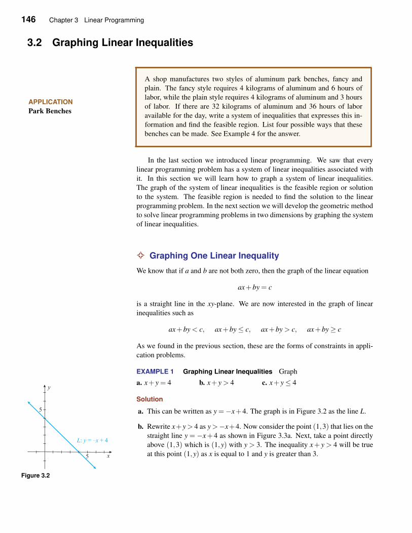
146 Chapter 3 Linear Programming
3.2 Graphing Linear Inequalities
APPLICATION
Park Benches
A shop manufactures two styles of aluminum park benches, fancy and
plain. The fancy style requires 4 kilograms of aluminum and 6 hours of
labor, while the plain style requires 4 kilograms of aluminum and 3 hours
of labor. If there are 32 kilograms of aluminum and 36 hours of labor
available for the day, write a system of inequalities that expresses this in-
formation and find the feasible region. List four possible ways that these
benches can be made. See Example 4 for the answer.
In the last section we introduced linear programming. We saw that every
linear programming problem has a system of linear inequalities associated with
it. In this section we will learn how to graph a system of linear inequalities.
The graph of the system of linear inequalities is the feasible region or solution
to the system. The feasible region is needed to find the solution to the linear
programming problem. In the next section we will develop the geometric method
to solve linear programming problems in two dimensions by graphing the system
of linear inequalities.
✧ Graphing One Linear Inequality
We know that if a and b are not both zero, then the graph of the linear equation
ax+by = c
is a straight line in the xy-plane. We are now interested in the graph of linear
inequalities such as
ax+by < c, ax+by≤ c, ax+by > c, ax+by≥ c
As we found in the previous section, these are the forms of constraints in appli-
cation problems.
EXAMPLE 1 Graphing Linear Inequalities Graph
a. x+ y = 4 b. x+ y > 4 c. x+ y≤ 4
Solution
a. This can be written as y =−x+4. The graph is in Figure 3.2 as the line L.
Figure 3.2
b. Rewrite x+y > 4 as y >−x+4. Now consider the point (1,3) that lies on the
straight line y = −x+ 4 as shown in Figure 3.3a. Next, take a point directly
above (1,3) which is (1,y) with y > 3. The inequality x+ y > 4 will be true
at this point (1,y) as x is equal to 1 and y is greater than 3.
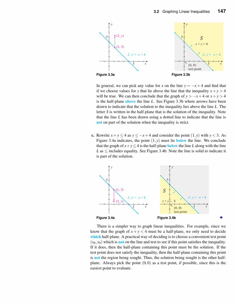
3.2 Graphing Linear Inequalities 147
Figure 3.3a Figure 3.3b
In general, we can pick any value for x on the line y = −x+ 4 and find that
if we choose values for y that lie above the line that the inequality x+ y > 4
will be true. We can then conclude that the graph of y >−x+4 or x+ y > 4
is the half-plane above the line L. See Figure 3.3b where arrows have been
drawn to indicate that the solution to the inequality lies above the line L. The
letter S is written in the half-plane that is the solution of the inequality. Note
that the line L has been drawn using a dotted line to indicate that the line is
not on part of the solution when the inequality is strict.
c. Rewrite x+ y≤ 4 as y≤−x+4 and consider the point (1,y) with y < 3. As
Figure 3.4a indicates, the point (1,y) must lie below the line. We conclude
that the graph of x+y≤ 4 is the half-plane below the line L along with the line
L as ≤ includes equality. See Figure 3.4b. Note the line is solid to indicate it
is part of the solution.
Figure 3.4a Figure 3.4b ✦
There is a simpler way to graph linear inequalities. For example, since we
know that the graph of x+ y < 4 must be a half-plane, we only need to decide
which half-plane. A practical way of deciding is to choose a convenient test point
(x0,y0) which is not on the line and test to see if this point satisfies the inequality.
If it does, then the half-plane containing this point must be the solution. If the
test point does not satisfy the inequality, then the half-plane containing this point
is not the region being sought. Thus, the solution being sought is the other half-
plane. Always pick the point (0,0) as a test point, if possible, since this is the
easiest point to evaluate.
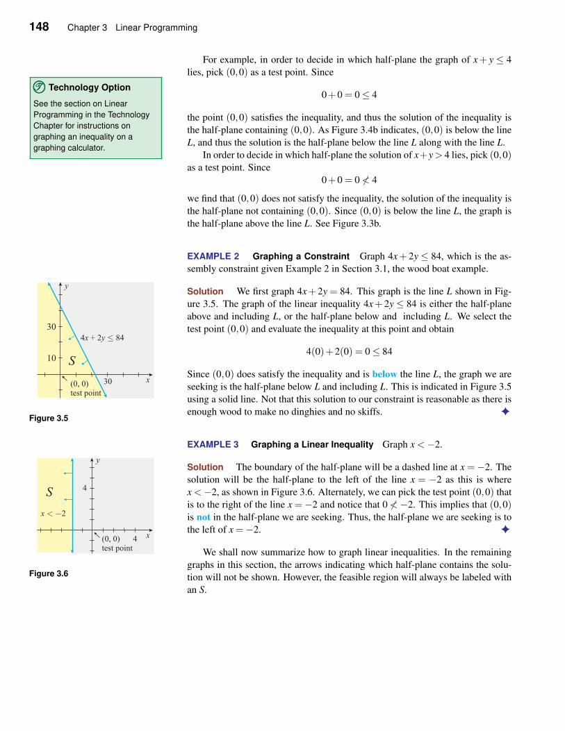
148 Chapter 3 Linear Programming
For example, in order to decide in which half-plane the graph of x+ y ≤ 4
lies, pick (0,0) as a test point. Since
0+0 = 0≤ 4
the point (0,0) satisfies the inequality, and thus the solution of the inequality is
TTT©©© Technology Option
See the section on Linear
Programming in the Technology
Chapter for instructions on
graphing an inequality on a
graphing calculator.
the half-plane containing (0,0). As Figure 3.4b indicates, (0,0) is below the line
L, and thus the solution is the half-plane below the line L along with the line L.
In order to decide in which half-plane the solution of x+y> 4 lies, pick (0,0)as a test point. Since
0+0 = 0 6< 4
we find that (0,0) does not satisfy the inequality, the solution of the inequality is
the half-plane not containing (0,0). Since (0,0) is below the line L, the graph is
the half-plane above the line L. See Figure 3.3b.
EXAMPLE 2 Graphing a Constraint Graph 4x+ 2y ≤ 84, which is the as-
sembly constraint given Example 2 in Section 3.1, the wood boat example.
Solution We first graph 4x+ 2y = 84. This graph is the line L shown in Fig-
ure 3.5. The graph of the linear inequality 4x+ 2y ≤ 84 is either the half-plane
above and including L, or the half-plane below and including L. We select the
Figure 3.5
test point (0,0) and evaluate the inequality at this point and obtain
4(0)+2(0) = 0≤ 84
Since (0,0) does satisfy the inequality and is below the line L, the graph we are
seeking is the half-plane below L and including L. This is indicated in Figure 3.5
using a solid line. Not that this solution to our constraint is reasonable as there is
enough wood to make no dinghies and no skiffs. ✦
EXAMPLE 3 Graphing a Linear Inequality Graph x <−2.
Solution The boundary of the half-plane will be a dashed line at x =−2. The
solution will be the half-plane to the left of the line x = −2 as this is where
x <−2, as shown in Figure 3.6. Alternately, we can pick the test point (0,0) that
Figure 3.6
is to the right of the line x =−2 and notice that 0 6<−2. This implies that (0,0)is not in the half-plane we are seeking. Thus, the half-plane we are seeking is to
the left of x =−2. ✦
We shall now summarize how to graph linear inequalities. In the remaining
graphs in this section, the arrows indicating which half-plane contains the solu-
tion will not be shown. However, the feasible region will always be labeled with
an S.
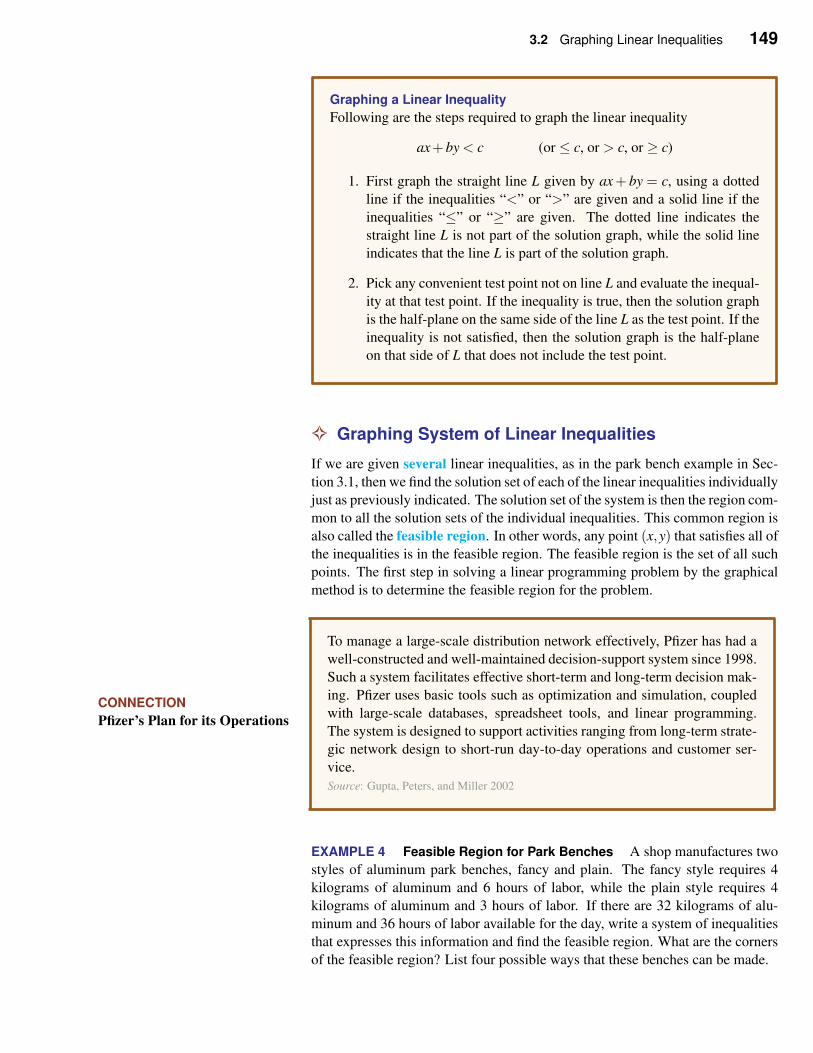
3.2 Graphing Linear Inequalities 149
Graphing a Linear Inequality
Following are the steps required to graph the linear inequality
ax+by < c (or ≤ c, or > c, or ≥ c)
1. First graph the straight line L given by ax+ by = c, using a dotted
line if the inequalities “<” or “>” are given and a solid line if the
inequalities “≤” or “≥” are given. The dotted line indicates the
straight line L is not part of the solution graph, while the solid line
indicates that the line L is part of the solution graph.
2. Pick any convenient test point not on line L and evaluate the inequal-
ity at that test point. If the inequality is true, then the solution graph
is the half-plane on the same side of the line L as the test point. If the
inequality is not satisfied, then the solution graph is the half-plane
on that side of L that does not include the test point.
✧ Graphing System of Linear Inequalities
If we are given several linear inequalities, as in the park bench example in Sec-
tion 3.1, then we find the solution set of each of the linear inequalities individually
just as previously indicated. The solution set of the system is then the region com-
mon to all the solution sets of the individual inequalities. This common region is
also called the feasible region. In other words, any point (x,y) that satisfies all of
the inequalities is in the feasible region. The feasible region is the set of all such
points. The first step in solving a linear programming problem by the graphical
method is to determine the feasible region for the problem.
CONNECTION
Pfizer’s Plan for its Operations
To manage a large-scale distribution network effectively, Pfizer has had a
well-constructed and well-maintained decision-support system since 1998.
Such a system facilitates effective short-term and long-term decision mak-
ing. Pfizer uses basic tools such as optimization and simulation, coupled
with large-scale databases, spreadsheet tools, and linear programming.
The system is designed to support activities ranging from long-term strate-
gic network design to short-run day-to-day operations and customer ser-
vice.
Source: Gupta, Peters, and Miller 2002
EXAMPLE 4 Feasible Region for Park Benches A shop manufactures two
styles of aluminum park benches, fancy and plain. The fancy style requires 4
kilograms of aluminum and 6 hours of labor, while the plain style requires 4
kilograms of aluminum and 3 hours of labor. If there are 32 kilograms of alu-
minum and 36 hours of labor available for the day, write a system of inequalities
that expresses this information and find the feasible region. What are the corners
of the feasible region? List four possible ways that these benches can be made.
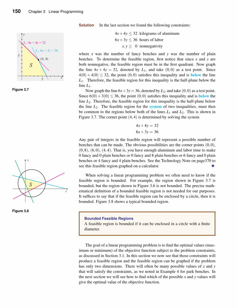
150 Chapter 3 Linear Programming
Solution In the last section we found the following constraints:
4x+4y ≤ 32 kilograms of aluminum
6x+3y ≤ 36 hours of labor
x,y ≥ 0 nonnegativity
where x was the number of fancy benches and y was the number of plain
benches. To determine the feasible region, first notice that since x and y are
both nonnegative, the feasible region must be in the first quadrant. Now graph
the line 4x + 4y = 32, denoted by L1, and take (0,0) as a test point. Since
4(0)+ 4(0) ≤ 32, the point (0,0) satisfies this inequality and is below the line
L1. Therefore, the feasible region for this inequality is the half-plane below the
Figure 3.7line L1.
Now graph the line 6x+3y= 36, denoted by L2, and take (0,0) as a test point.
Since 6(0)+3(0)≤ 36, the point (0,0) satisfies this inequality and is below the
line L2. Therefore, the feasible region for this inequality is the half-plane below
the line L2. The feasible region for the system of two inequalities, must then
be common to the regions below both of the lines L1 and L2. This is shown in
Figure 3.7. The corner point (4,4) is determined by solving the system
4x+4y = 32
6x+3y = 36
Any pair of integers in the feasible region will represent a possible number of
benches that can be made. The obvious possibilities are the corner points (0,0),(0,8), (6,0), (4,4). That is, you have enough aluminum and labor time to make
0 fancy and 0 plain benches or 0 fancy and 8 plain benches or 6 fancy and 0 plain
benches or 4 fancy and 4 plain benches. See the Technology Note on page370 to
see this feasible region graphed on a calculator. ✦
When solving a linear programming problem we often need to know if the
feasible region is bounded. For example, the region shown in Figure 3.7 is
bounded, but the region shown in Figure 3.6 is not bounded. The precise math-
ematical definition of a bounded feasible region is not needed for our purposes.
It suffices to say that if the feasible region can be enclosed by a circle, then it is
bounded. Figure 3.8 shows a typical bounded region.
Figure 3.8
Bounded Feasible Regions
A feasible region is bounded if it can be enclosed in a circle with a finite
diameter.
The goal of a linear programming problem is to find the optimal values (max-
imum or minimum) of the objective function subject to the problem constraints,
as discussed in Section 3.1. In this section we now see that those constraints will
produce a feasible region and the feasible region can be graphed if the problem
has only two dimensions. There will often be many possible values of x and y
that will satisfy the constraints, as we noted in Example 4 for park benches. In
the next section we will see how to find which of the possible x and y values will
give the optimal value of the objective function.
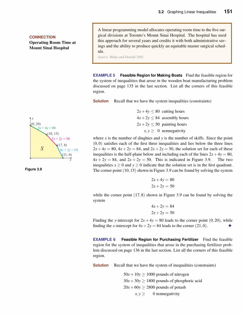
3.2 Graphing Linear Inequalities 151
CONNECTION
Operating Room Time at
Mount Sinai Hospital
A linear programming model allocates operating room time to the five sur-
gical divisions at Toronto’s Mount Sinai Hospital. The hospital has used
this approach for several years and credits it with both administrative sav-
ings and the ability to produce quickly an equitable master surgical sched-
ule.
Source: Blake and Donald 2002
EXAMPLE 5 Feasible Region for Making Boats Find the feasible region for
the system of inequalities that arose in the wooden boat manufacturing problem
discussed on page 135 in the last section. List all the corners of this feasible
region.
Solution Recall that we have the system inequalities (constraints)
2x+4y ≤ 80 cutting hours
4x+2y ≤ 84 assembly hours
2x+2y ≤ 50 painting hours
x,y ≥ 0 nonnegativity
where x is the number of dinghies and y is the number of skiffs. Since the point
(0,0) satisfies each of the first three inequalities and lies below the three lines
2x+ 4y = 80, 4x+ 2y = 84, and 2x+ 2y = 50, the solution set for each of these
inequalities is the half-plane below and including each of the lines 2x+4y = 80,
4x + 2y = 84, and 2x + 2y = 50. This is indicated in Figure 3.9. The two
Figure 3.9inequalities x ≥ 0 and y ≥ 0 indicate that the solution set is in the first quadrant.
The corner point (10,15) shown in Figure 3.9 can be found by solving the system
2x+4y = 80
2x+2y = 50
while the corner point (17,8) shown in Figure 3.9 can be found by solving the
system
4x+2y = 84
2x+2y = 50
Finding the y-intercept for 2x+ 4y = 80 leads to the corner point (0,20), while
finding the x-intercept for 4x+2y = 84 leads to the corner (21,0). ✦
EXAMPLE 6 Feasible Region for Purchasing Fertilizer Find the feasible
region for the system of inequalities that arose in the purchasing fertilizer prob-
lem discussed on page 136 in the last section. List all the corners of this feasible
region.
Solution Recall that we have the system of inequalities (constraints)
50x+10y ≥ 1000 pounds of nitrogen
30x+30y ≥ 1800 pounds of phosphoric acid
20x+60y ≥ 2800 pounds of potash
x,y ≥ 0 nonnegativity
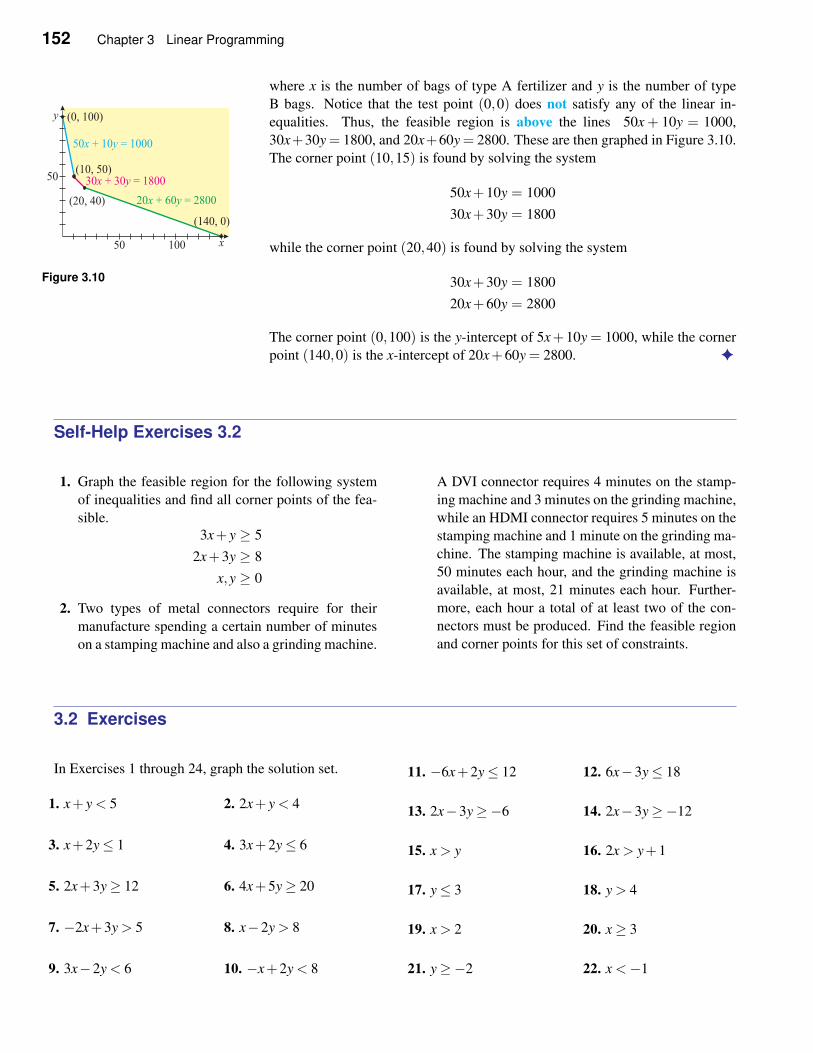
152 Chapter 3 Linear Programming
where x is the number of bags of type A fertilizer and y is the number of type
B bags. Notice that the test point (0,0) does not satisfy any of the linear in-
equalities. Thus, the feasible region is above the lines 50x + 10y = 1000,
Figure 3.10
30x+30y = 1800, and 20x+60y = 2800. These are then graphed in Figure 3.10.
The corner point (10,15) is found by solving the system
50x+10y = 1000
30x+30y = 1800
while the corner point (20,40) is found by solving the system
30x+30y = 1800
20x+60y = 2800
The corner point (0,100) is the y-intercept of 5x+10y = 1000, while the corner
point (140,0) is the x-intercept of 20x+60y = 2800. ✦
Self-Help Exercises 3.2
1. Graph the feasible region for the following system
of inequalities and find all corner points of the fea-
sible.
3x+ y ≥ 5
2x+3y ≥ 8
x,y ≥ 0
2. Two types of metal connectors require for their
manufacture spending a certain number of minutes
on a stamping machine and also a grinding machine.
A DVI connector requires 4 minutes on the stamp-
ing machine and 3 minutes on the grinding machine,
while an HDMI connector requires 5 minutes on the
stamping machine and 1 minute on the grinding ma-
chine. The stamping machine is available, at most,
50 minutes each hour, and the grinding machine is
available, at most, 21 minutes each hour. Further-
more, each hour a total of at least two of the con-
nectors must be produced. Find the feasible region
and corner points for this set of constraints.
3.2 Exercises
In Exercises 1 through 24, graph the solution set.
1. x+ y < 5 2. 2x+ y < 4
3. x+2y≤ 1 4. 3x+2y≤ 6
5. 2x+3y≥ 12 6. 4x+5y≥ 20
7. −2x+3y > 5 8. x−2y > 8
9. 3x−2y < 6 10. −x+2y < 8
11. −6x+2y≤ 12 12. 6x−3y≤ 18
13. 2x−3y≥−6 14. 2x−3y≥−12
15. x > y 16. 2x > y+1
17. y≤ 3 18. y > 4
19. x > 2 20. x≥ 3
21. y≥−2 22. x <−1
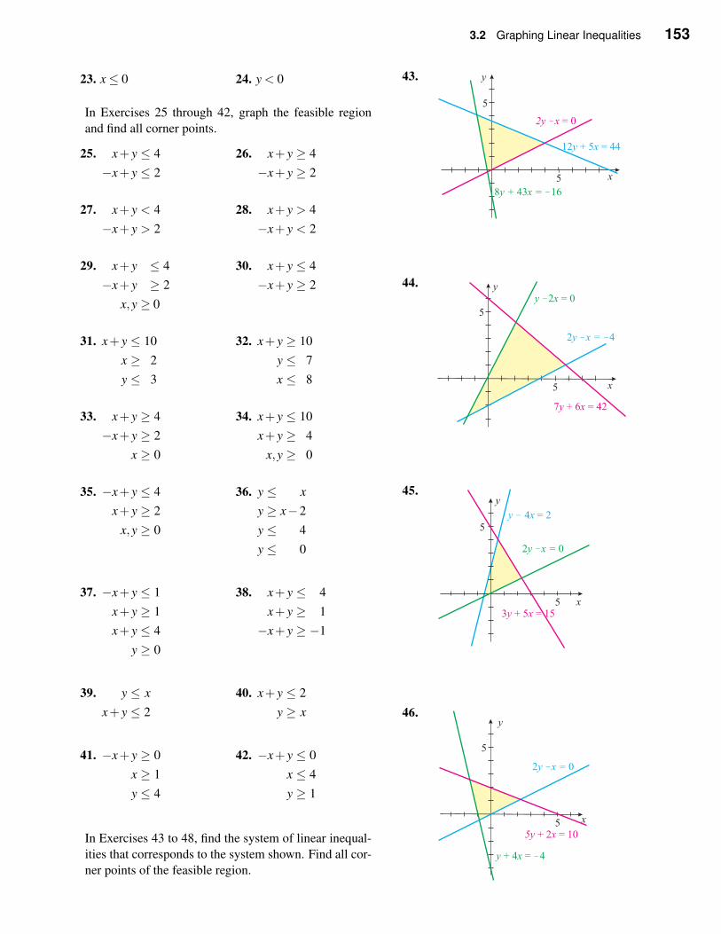
3.2 Graphing Linear Inequalities 153
23. x≤ 0 24. y < 0
In Exercises 25 through 42, graph the feasible region
and find all corner points.
25. x+ y ≤ 4
−x+ y ≤ 2
26. x+ y ≥ 4
−x+ y ≥ 2
27. x+ y < 4
−x+ y > 2
28. x+ y > 4
−x+ y < 2
29. x+ y ≤ 4
−x+ y ≥ 2
x,y ≥ 0
30. x+ y ≤ 4
−x+ y ≥ 2
31. x+ y ≤ 10
x ≥ 2
y ≤ 3
32. x+ y ≥ 10
y ≤ 7
x ≤ 8
33. x+ y ≥ 4
−x+ y ≥ 2
x ≥ 0
34. x+ y ≤ 10
x+ y ≥ 4
x,y ≥ 0
35. −x+ y ≤ 4
x+ y ≥ 2
x,y ≥ 0
36. y ≤ x
y ≥ x−2
y ≤ 4
y ≤ 0
37. −x+ y ≤ 1
x+ y ≥ 1
x+ y ≤ 4
y ≥ 0
38. x+ y ≤ 4
x+ y ≥ 1
−x+ y ≥ −1
39. y ≤ x
x+ y ≤ 2
40. x+ y ≤ 2
y ≥ x
41. −x+ y ≥ 0
x ≥ 1
y ≤ 4
42. −x+ y ≤ 0
x ≤ 4
y ≥ 1
In Exercises 43 to 48, find the system of linear inequal-
ities that corresponds to the system shown. Find all cor-
ner points of the feasible region.
43.
44.
45.
46.
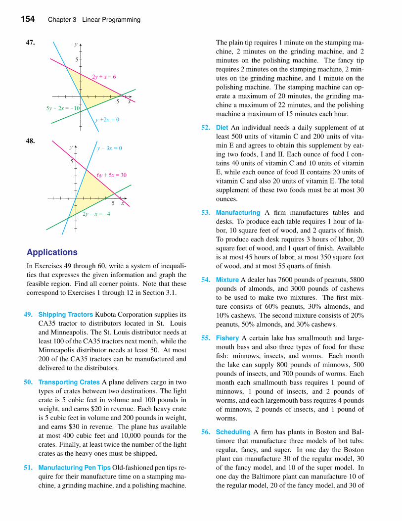
154 Chapter 3 Linear Programming
47.
48.
Applications
In Exercises 49 through 60, write a system of inequali-
ties that expresses the given information and graph the
feasible region. Find all corner points. Note that these
correspond to Exercises 1 through 12 in Section 3.1.
49. Shipping Tractors Kubota Corporation supplies its
CA35 tractor to distributors located in St. Louis
and Minneapolis. The St. Louis distributor needs at
least 100 of the CA35 tractors next month, while the
Minneapolis distributor needs at least 50. At most
200 of the CA35 tractors can be manufactured and
delivered to the distributors.
50. Transporting Crates A plane delivers cargo in two
types of crates between two destinations. The light
crate is 5 cubic feet in volume and 100 pounds in
weight, and earns $20 in revenue. Each heavy crate
is 5 cubic feet in volume and 200 pounds in weight,
and earns $30 in revenue. The plane has available
at most 400 cubic feet and 10,000 pounds for the
crates. Finally, at least twice the number of the light
crates as the heavy ones must be shipped.
51. Manufacturing Pen Tips Old-fashioned pen tips re-
quire for their manufacture time on a stamping ma-
chine, a grinding machine, and a polishing machine.
The plain tip requires 1 minute on the stamping ma-
chine, 2 minutes on the grinding machine, and 2
minutes on the polishing machine. The fancy tip
requires 2 minutes on the stamping machine, 2 min-
utes on the grinding machine, and 1 minute on the
polishing machine. The stamping machine can op-
erate a maximum of 20 minutes, the grinding ma-
chine a maximum of 22 minutes, and the polishing
machine a maximum of 15 minutes each hour.
52. Diet An individual needs a daily supplement of at
least 500 units of vitamin C and 200 units of vita-
min E and agrees to obtain this supplement by eat-
ing two foods, I and II. Each ounce of food I con-
tains 40 units of vitamin C and 10 units of vitamin
E, while each ounce of food II contains 20 units of
vitamin C and also 20 units of vitamin E. The total
supplement of these two foods must be at most 30
ounces.
53. Manufacturing A firm manufactures tables and
desks. To produce each table requires 1 hour of la-
bor, 10 square feet of wood, and 2 quarts of finish.
To produce each desk requires 3 hours of labor, 20
square feet of wood, and 1 quart of finish. Available
is at most 45 hours of labor, at most 350 square feet
of wood, and at most 55 quarts of finish.
54. Mixture A dealer has 7600 pounds of peanuts, 5800
pounds of almonds, and 3000 pounds of cashews
to be used to make two mixtures. The first mix-
ture consists of 60% peanuts, 30% almonds, and
10% cashews. The second mixture consists of 20%
peanuts, 50% almonds, and 30% cashews.
55. Fishery A certain lake has smallmouth and large-
mouth bass and also three types of food for these
fish: minnows, insects, and worms. Each month
the lake can supply 800 pounds of minnows, 500
pounds of insects, and 700 pounds of worms. Each
month each smallmouth bass requires 1 pound of
minnows, 1 pound of insects, and 2 pounds of
worms, and each largemouth bass requires 4 pounds
of minnows, 2 pounds of insects, and 1 pound of
worms.
56. Scheduling A firm has plants in Boston and Bal-
timore that manufacture three models of hot tubs:
regular, fancy, and super. In one day the Boston
plant can manufacture 30 of the regular model, 30
of the fancy model, and 10 of the super model. In
one day the Baltimore plant can manufacture 10 of
the regular model, 20 of the fancy model, and 30 of
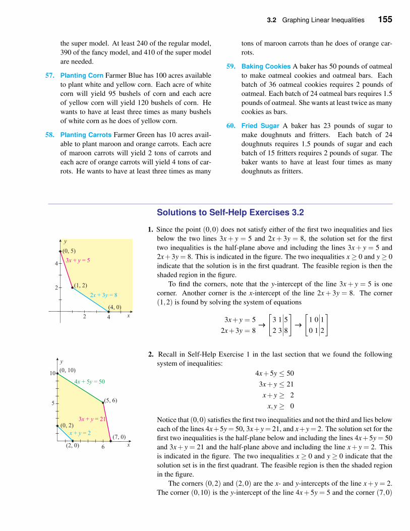
3.2 Graphing Linear Inequalities 155
the super model. At least 240 of the regular model,
390 of the fancy model, and 410 of the super model
are needed.
57. Planting Corn Farmer Blue has 100 acres available
to plant white and yellow corn. Each acre of white
corn will yield 95 bushels of corn and each acre
of yellow corn will yield 120 bushels of corn. He
wants to have at least three times as many bushels
of white corn as he does of yellow corn.
58. Planting Carrots Farmer Green has 10 acres avail-
able to plant maroon and orange carrots. Each acre
of maroon carrots will yield 2 tons of carrots and
each acre of orange carrots will yield 4 tons of car-
rots. He wants to have at least three times as many
tons of maroon carrots than he does of orange car-
rots.
59. Baking Cookies A baker has 50 pounds of oatmeal
to make oatmeal cookies and oatmeal bars. Each
batch of 36 oatmeal cookies requires 2 pounds of
oatmeal. Each batch of 24 oatmeal bars requires 1.5
pounds of oatmeal. She wants at least twice as many
cookies as bars.
60. Fried Sugar A baker has 23 pounds of sugar to
make doughnuts and fritters. Each batch of 24
doughnuts requires 1.5 pounds of sugar and each
batch of 15 fritters requires 2 pounds of sugar. The
baker wants to have at least four times as many
doughnuts as fritters.
Solutions to Self-Help Exercises 3.2
1. Since the point (0,0) does not satisfy either of the first two inequalities and lies
below the two lines 3x + y = 5 and 2x + 3y = 8, the solution set for the first
two inequalities is the half-plane above and including the lines 3x+ y = 5 and
2x+3y = 8. This is indicated in the figure. The two inequalities x≥ 0 and y≥ 0
indicate that the solution is in the first quadrant. The feasible region is then the
shaded region in the figure.
To find the corners, note that the y-intercept of the line 3x+ y = 5 is one
corner. Another corner is the x-intercept of the line 2x+ 3y = 8. The corner
(1,2) is found by solving the system of equations
3x+ y = 5
2x+3y = 8→→→[
3 1 5
2 3 8
]
→→→[
1 0 1
0 1 2
]
2. Recall in Self-Help Exercise 1 in the last section that we found the following
system of inequalities:
4x+5y ≤ 50
3x+ y ≤ 21
x+ y ≥ 2
x,y ≥ 0
Notice that (0,0) satisfies the first two inequalities and not the third and lies below
each of the lines 4x+5y = 50, 3x+y = 21, and x+y = 2. The solution set for the
first two inequalities is the half-plane below and including the lines 4x+5y = 50
and 3x+ y = 21 and the half-plane above and including the line x+ y = 2. This
is indicated in the figure. The two inequalities x ≥ 0 and y ≥ 0 indicate that the
solution set is in the first quadrant. The feasible region is then the shaded region
in the figure.
The corners (0,2) and (2,0) are the x- and y-intercepts of the line x+ y = 2.
The corner (0,10) is the y-intercept of the line 4x+5y = 5 and the corner (7,0)
156 Chapter 3 Linear Programming
is the x-intercept of the line 3x+ y = 21. Finally the corner (5,6) is found by
solving the system of equations
4x+5y = 50
3x+ y = 21→→→[
4 5 50
3 1 21
]
→→→[
1 0 5
0 1 6
]
3.3 Graphical Solution of Linear Programming Problems
APPLICATION
Minimizing Costs
A farmer can buy two types of 100-pound bags of fertilizer, type A and
type B. Each 100-pound bag of type A fertilizer costs $20 and contains
50 pounds of nitrogen, 30 pounds of phosphoric acid, and 20 pounds of
potash, whereas each 100-pound bag of type B fertilizer costs $30 and
contains 10 pounds of nitrogen, 30 pounds of phosphoric acid, and 60
pounds of potash. The farmer requires at least 1000 pounds of nitrogen,
1800 pounds of phosphoric acid, and 2800 pounds of potash. How many
bags of each type of fertilizer should be purchased in order to minimize
cost? The answer is found in Example 5.
✧ Some Linear Programming Problems
We have seen how business, economics, finance, and many other areas are re-
plete with complex decision or allocation problems that involve the selection of
specific values of many interrelated variables. We saw that there is a specific
objective function that is to be maximized or minimized and we saw examples
of such objectives as profit, revenue, cost, expected return on an investment, and
even some measure of social welfare. The variables are normally subject to con-
straints that take the form of a set of inequalities that give rise to a feasible re-
gion. Maximizing or minimizing the objective function in the feasible region was
called linear programming. In this section we see how to solve problems with a
small number of variables using a geometric approach. In another chapter we
will find an alternative method that can be used to solve the most complex linear
programming problems and does not rely on the graph of the feasible region.
EXAMPLE 1 Profit and the Feasible Region for Making Boats Suppose the
small, wooden-boat manufacturer of the last two sections obtained a profit of $60
for every dinghy manufactured and $80 for every skiff. How many of each type
of boat should be made in order to maximize the profits?
Solution If x is the number of dinghies manufactured each week and y the
number of skiffs, then the profit in dollars is P = 60x+ 80y. Recalling the con-
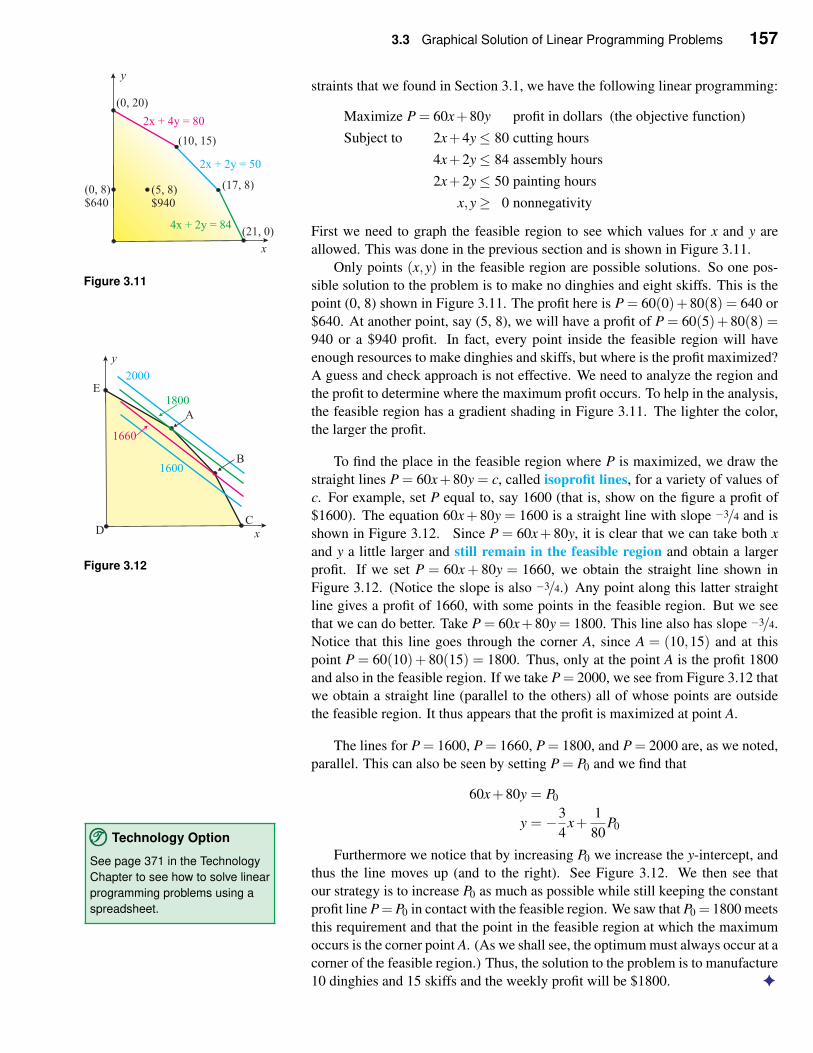
3.3 Graphical Solution of Linear Programming Problems 157
straints that we found in Section 3.1, we have the following linear programming:
Maximize P = 60x+80y profit in dollars (the objective function)
Subject to 2x+4y≤ 80 cutting hours
4x+2y≤ 84 assembly hours
2x+2y≤ 50 painting hours
x,y≥ 0 nonnegativity
First we need to graph the feasible region to see which values for x and y are
allowed. This was done in the previous section and is shown in Figure 3.11.
Figure 3.11Only points (x,y) in the feasible region are possible solutions. So one pos-
sible solution to the problem is to make no dinghies and eight skiffs. This is the
point (0, 8) shown in Figure 3.11. The profit here is P = 60(0)+80(8) = 640 or
$640. At another point, say (5, 8), we will have a profit of P = 60(5)+80(8) =940 or a $940 profit. In fact, every point inside the feasible region will have
enough resources to make dinghies and skiffs, but where is the profit maximized?
A guess and check approach is not effective. We need to analyze the region and
the profit to determine where the maximum profit occurs. To help in the analysis,
the feasible region has a gradient shading in Figure 3.11. The lighter the color,
the larger the profit.
To find the place in the feasible region where P is maximized, we draw the
straight lines P = 60x+80y = c, called isoprofit lines, for a variety of values of
c. For example, set P equal to, say 1600 (that is, show on the figure a profit of
$1600). The equation 60x+ 80y = 1600 is a straight line with slope −3/4 and is
shown in Figure 3.12. Since P = 60x+ 80y, it is clear that we can take both x
Figure 3.12and y a little larger and still remain in the feasible region and obtain a larger
profit. If we set P = 60x + 80y = 1660, we obtain the straight line shown in
Figure 3.12. (Notice the slope is also −3/4.) Any point along this latter straight
line gives a profit of 1660, with some points in the feasible region. But we see
that we can do better. Take P = 60x+80y = 1800. This line also has slope −3/4.
Notice that this line goes through the corner A, since A = (10,15) and at this
point P = 60(10)+ 80(15) = 1800. Thus, only at the point A is the profit 1800
and also in the feasible region. If we take P = 2000, we see from Figure 3.12 that
we obtain a straight line (parallel to the others) all of whose points are outside
the feasible region. It thus appears that the profit is maximized at point A.
The lines for P = 1600, P = 1660, P = 1800, and P = 2000 are, as we noted,
parallel. This can also be seen by setting P = P0 and we find that
60x+80y = P0
y = −3
4x+
1
80P0
Furthermore we notice that by increasing P0 we increase the y-intercept, and
thus the line moves up (and to the right). See Figure 3.12. We then see that
TTT©©© Technology Option
See page 371 in the Technology
Chapter to see how to solve linear
programming problems using a
spreadsheet.
our strategy is to increase P0 as much as possible while still keeping the constant
profit line P=P0 in contact with the feasible region. We saw that P0 = 1800 meets
this requirement and that the point in the feasible region at which the maximum
occurs is the corner point A. (As we shall see, the optimum must always occur at a
corner of the feasible region.) Thus, the solution to the problem is to manufacture
10 dinghies and 15 skiffs and the weekly profit will be $1800. ✦
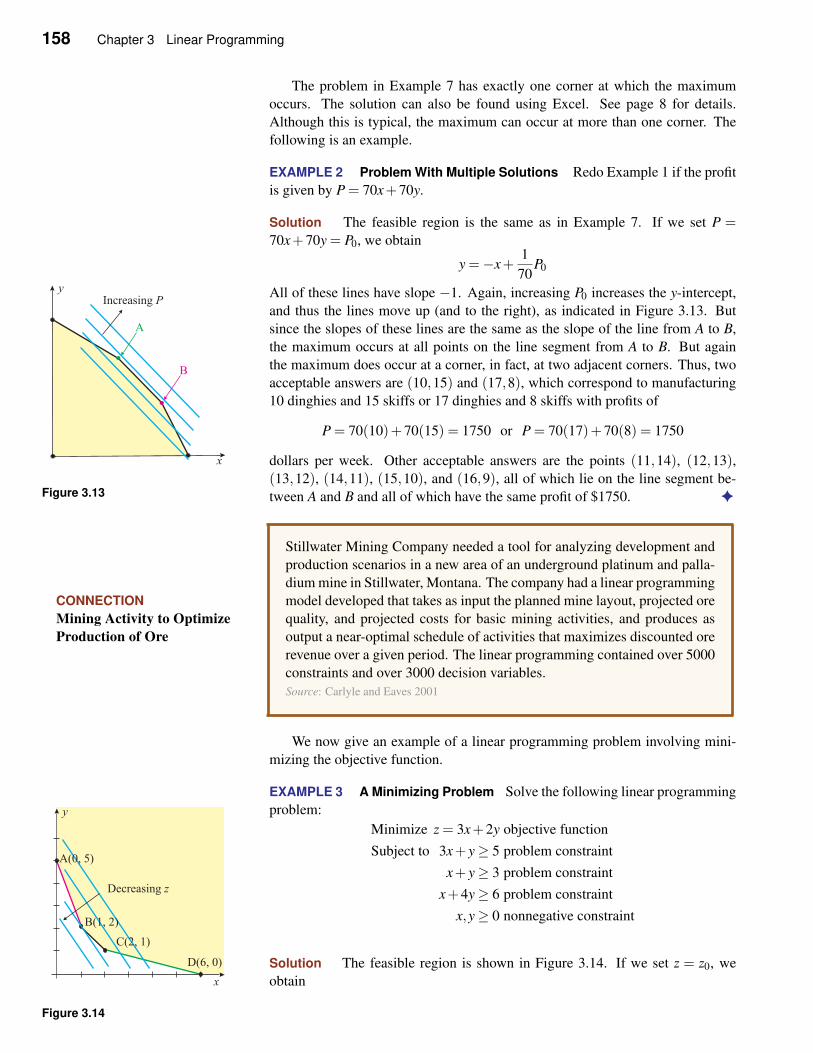
158 Chapter 3 Linear Programming
The problem in Example 7 has exactly one corner at which the maximum
occurs. The solution can also be found using Excel. See page 8 for details.
Although this is typical, the maximum can occur at more than one corner. The
following is an example.
EXAMPLE 2 Problem With Multiple Solutions Redo Example 1 if the profit
is given by P = 70x+70y.
Solution The feasible region is the same as in Example 7. If we set P =70x+70y = P0, we obtain
y =−x+1
70P0
All of these lines have slope −1. Again, increasing P0 increases the y-intercept,
and thus the lines move up (and to the right), as indicated in Figure 3.13. But
since the slopes of these lines are the same as the slope of the line from A to B,
the maximum occurs at all points on the line segment from A to B. But again
the maximum does occur at a corner, in fact, at two adjacent corners. Thus, two
acceptable answers are (10,15) and (17,8), which correspond to manufacturing
10 dinghies and 15 skiffs or 17 dinghies and 8 skiffs with profits of
P = 70(10)+70(15) = 1750 or P = 70(17)+70(8) = 1750
dollars per week. Other acceptable answers are the points (11,14), (12,13),
Figure 3.13(13,12), (14,11), (15,10), and (16,9), all of which lie on the line segment be-
tween A and B and all of which have the same profit of $1750. ✦
CONNECTION
Mining Activity to Optimize
Production of Ore
Stillwater Mining Company needed a tool for analyzing development and
production scenarios in a new area of an underground platinum and palla-
dium mine in Stillwater, Montana. The company had a linear programming
model developed that takes as input the planned mine layout, projected ore
quality, and projected costs for basic mining activities, and produces as
output a near-optimal schedule of activities that maximizes discounted ore
revenue over a given period. The linear programming contained over 5000
constraints and over 3000 decision variables.
Source: Carlyle and Eaves 2001
We now give an example of a linear programming problem involving mini-
mizing the objective function.
EXAMPLE 3 A Minimizing Problem Solve the following linear programming
problem:
Minimize z = 3x+2y objective function
Subject to 3x+ y≥ 5 problem constraint
x+ y≥ 3 problem constraint
x+4y≥ 6 problem constraint
x,y≥ 0 nonnegative constraint
Solution The feasible region is shown in Figure 3.14. If we set z = z0, we
obtain
Figure 3.14
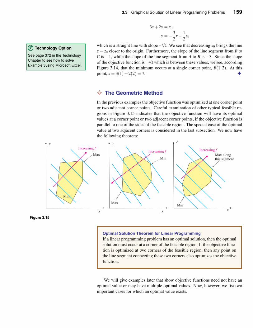
3.3 Graphical Solution of Linear Programming Problems 159
3x+2y = z0
y = −3
2x+
1
2z0
which is a straight line with slope −3/2. We see that decreasing z0 brings the line
z = z0 closer to the origin. Furthermore, the slope of the line segment from B to
C is −1, while the slope of the line segment from A to B is −3. Since the slope
TTT©©© Technology Option
See page 372 in the Technology
Chapter to see how to solve
Example 3using Microsoft Excel.of the objective function is −3/2 which is between these values, we see, according
Figure 3.14, that the minimum occurs at a single corner point, B(1,2). At this
point, z = 3(1)+2(2) = 7. ✦
✧ The Geometric Method
In the previous examples the objective function was optimized at one corner point
or two adjacent corner points. Careful examination of other typical feasible re-
gions in Figure 3.15 indicates that the objective function will have its optimal
values at a corner point or two adjacent corner points, if the objective function is
parallel to one of the sides of the feasible region. The special case of the optimal
value at two adjacent corners is considered in the last subsection. We now have
the following theorem:
Figure 3.15
Optimal Solution Theorem for Linear Programming
If a linear programming problem has an optimal solution, then the optimal
solution must occur at a corner of the feasible region. If the objective func-
tion is optimized at two corners of the feasible region, then any point on
the line segment connecting these two corners also optimizes the objective
function.
We will give examples later that show objective functions need not have an
optimal value or may have multiple optimal values. Now, however, we list two
important cases for which an optimal value exists.
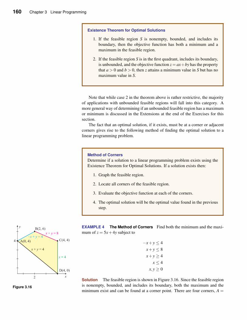
160 Chapter 3 Linear Programming
Existence Theorem for Optimal Solutions
1. If the feasible region S is nonempty, bounded, and includes its
boundary, then the objective function has both a minimum and a
maximum in the feasible region.
2. If the feasible region S is in the first quadrant, includes its boundary,
is unbounded, and the objective function z= ax+by has the property
that a > 0 and b > 0, then z attains a minimum value in S but has no
maximum value in S.
Note that while case 2 in the theorem above is rather restrictive, the majority
of applications with unbounded feasible regions will fall into this category. A
more general way of determining if an unbounded feasible region has a maximum
or minimum is discussed in the Extensions at the end of the Exercises for this
section.
The fact that an optimal solution, if it exists, must be at a corner or adjacent
corners gives rise to the following method of finding the optimal solution to a
linear programming problem.
Method of Corners
Determine if a solution to a linear programming problem exists using the
Existence Theorem for Optimal Solutions. If a solution exists then:
1. Graph the feasible region.
2. Locate all corners of the feasible region.
3. Evaluate the objective function at each of the corners.
4. The optimal solution will be the optimal value found in the previous
step.
EXAMPLE 4 The Method of Corners Find both the minimum and the maxi-
mum of z = 5x+4y subject to
Figure 3.16
−x+ y ≤ 4
x+ y ≤ 8
x+ y ≥ 4
x ≤ 4
x,y ≥ 0
Solution The feasible region is shown in Figure 3.16. Since the feasible region
is nonempty, bounded, and includes its boundary, both the maximum and the
minimum exist and can be found at a corner point. There are four corners, A =
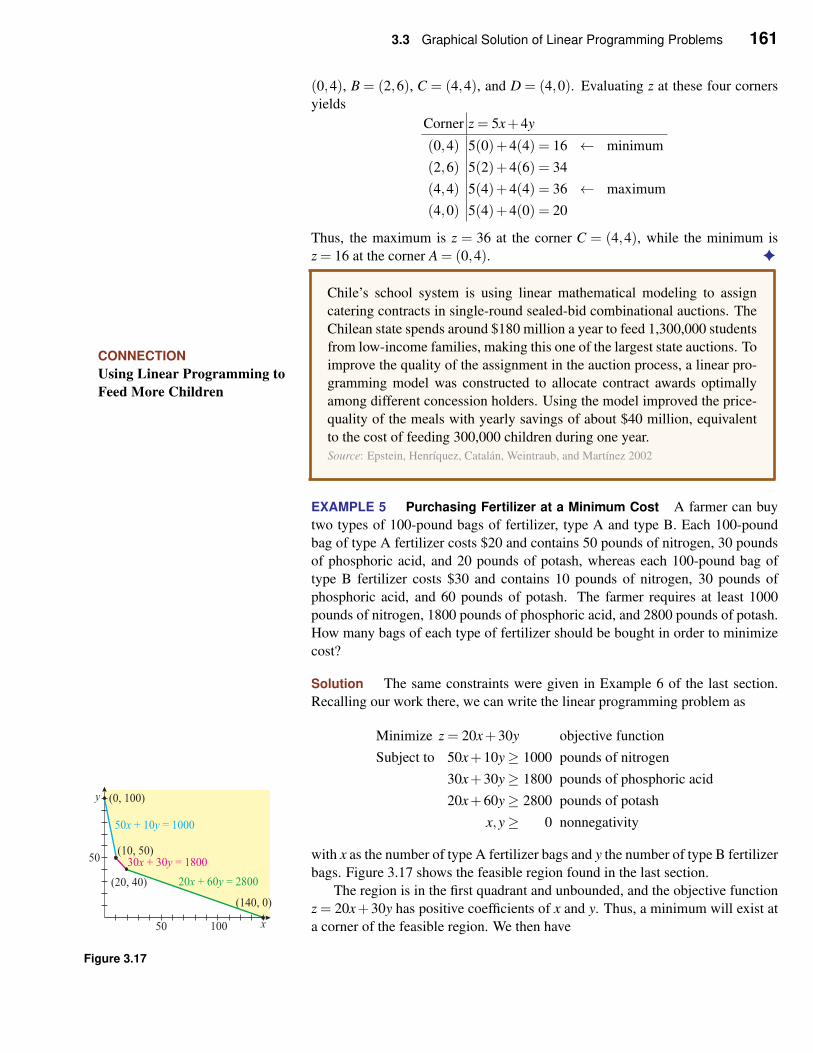
3.3 Graphical Solution of Linear Programming Problems 161
(0,4), B = (2,6), C = (4,4), and D = (4,0). Evaluating z at these four corners
yields
Corner z = 5x+4y
(0,4) 5(0)+4(4) = 16 ← minimum
(2,6) 5(2)+4(6) = 34
(4,4) 5(4)+4(4) = 36 ← maximum
(4,0) 5(4)+4(0) = 20
Thus, the maximum is z = 36 at the corner C = (4,4), while the minimum is
z = 16 at the corner A = (0,4). ✦
CONNECTION
Using Linear Programming to
Feed More Children
Chile’s school system is using linear mathematical modeling to assign
catering contracts in single-round sealed-bid combinational auctions. The
Chilean state spends around $180 million a year to feed 1,300,000 students
from low-income families, making this one of the largest state auctions. To
improve the quality of the assignment in the auction process, a linear pro-
gramming model was constructed to allocate contract awards optimally
among different concession holders. Using the model improved the price-
quality of the meals with yearly savings of about $40 million, equivalent
to the cost of feeding 300,000 children during one year.
Source: Epstein, Henríquez, Catalán, Weintraub, and Martínez 2002
EXAMPLE 5 Purchasing Fertilizer at a Minimum Cost A farmer can buy
two types of 100-pound bags of fertilizer, type A and type B. Each 100-pound
bag of type A fertilizer costs $20 and contains 50 pounds of nitrogen, 30 pounds
of phosphoric acid, and 20 pounds of potash, whereas each 100-pound bag of
type B fertilizer costs $30 and contains 10 pounds of nitrogen, 30 pounds of
phosphoric acid, and 60 pounds of potash. The farmer requires at least 1000
pounds of nitrogen, 1800 pounds of phosphoric acid, and 2800 pounds of potash.
How many bags of each type of fertilizer should be bought in order to minimize
cost?
Solution The same constraints were given in Example 6 of the last section.
Recalling our work there, we can write the linear programming problem as
Minimize z = 20x+30y objective function
Subject to 50x+10y≥ 1000 pounds of nitrogen
30x+30y≥ 1800 pounds of phosphoric acid
20x+60y≥ 2800 pounds of potash
x,y≥ 0 nonnegativity
with x as the number of type A fertilizer bags and y the number of type B fertilizer
bags. Figure 3.17 shows the feasible region found in the last section.
The region is in the first quadrant and unbounded, and the objective function
z = 20x+30y has positive coefficients of x and y. Thus, a minimum will exist at
a corner of the feasible region. We then have
Figure 3.17
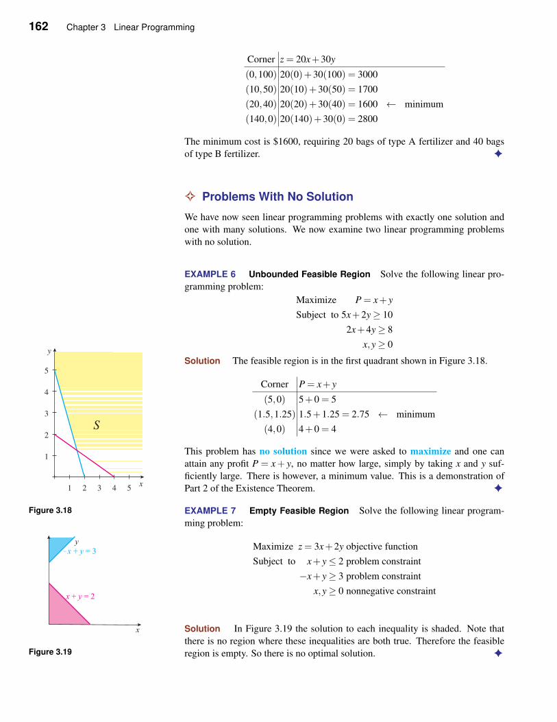
162 Chapter 3 Linear Programming
Corner z = 20x+30y
(0,100) 20(0)+30(100) = 3000
(10,50) 20(10)+30(50) = 1700
(20,40) 20(20)+30(40) = 1600 ← minimum
(140,0) 20(140)+30(0) = 2800
The minimum cost is $1600, requiring 20 bags of type A fertilizer and 40 bags
of type B fertilizer. ✦
✧ Problems With No Solution
We have now seen linear programming problems with exactly one solution and
one with many solutions. We now examine two linear programming problems
with no solution.
EXAMPLE 6 Unbounded Feasible Region Solve the following linear pro-
gramming problem:
Maximize P = x+ y
Subject to 5x+2y≥ 10
2x+4y≥ 8
x,y≥ 0
Solution The feasible region is in the first quadrant shown in Figure 3.18.
Corner P = x+ y
(5,0) 5+0 = 5
(1.5,1.25) 1.5+1.25 = 2.75 ← minimum
(4,0) 4+0 = 4
This problem has no solution since we were asked to maximize and one can
attain any profit P = x+ y, no matter how large, simply by taking x and y suf-
ficiently large. There is however, a minimum value. This is a demonstration of
Part 2 of the Existence Theorem. ✦x
y
S
1 2 3 4 5
1
2
3
4
5
Figure 3.18 EXAMPLE 7 Empty Feasible Region Solve the following linear program-
ming problem:
Figure 3.19
Maximize z = 3x+2y objective function
Subject to x+ y≤ 2 problem constraint
−x+ y≥ 3 problem constraint
x,y≥ 0 nonnegative constraint
Solution In Figure 3.19 the solution to each inequality is shaded. Note that
there is no region where these inequalities are both true. Therefore the feasible
region is empty. So there is no optimal solution. ✦
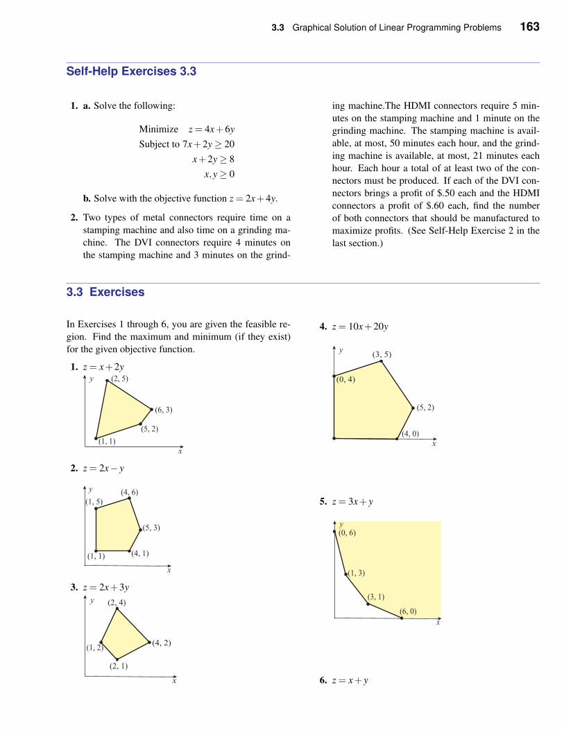
3.3 Graphical Solution of Linear Programming Problems 163
Self-Help Exercises 3.3
1. a. Solve the following:
Minimize z = 4x+6y
Subject to 7x+2y≥ 20
x+2y≥ 8
x,y≥ 0
b. Solve with the objective function z = 2x+4y.
2. Two types of metal connectors require time on a
stamping machine and also time on a grinding ma-
chine. The DVI connectors require 4 minutes on
the stamping machine and 3 minutes on the grind-
ing machine.The HDMI connectors require 5 min-
utes on the stamping machine and 1 minute on the
grinding machine. The stamping machine is avail-
able, at most, 50 minutes each hour, and the grind-
ing machine is available, at most, 21 minutes each
hour. Each hour a total of at least two of the con-
nectors must be produced. If each of the DVI con-
nectors brings a profit of $.50 each and the HDMI
connectors a profit of $.60 each, find the number
of both connectors that should be manufactured to
maximize profits. (See Self-Help Exercise 2 in the
last section.)
3.3 Exercises
In Exercises 1 through 6, you are given the feasible re-
gion. Find the maximum and minimum (if they exist)
for the given objective function.
1. z = x+2y
2. z = 2x− y
3. z = 2x+3y
4. z = 10x+20y
5. z = 3x+ y
6. z = x+ y
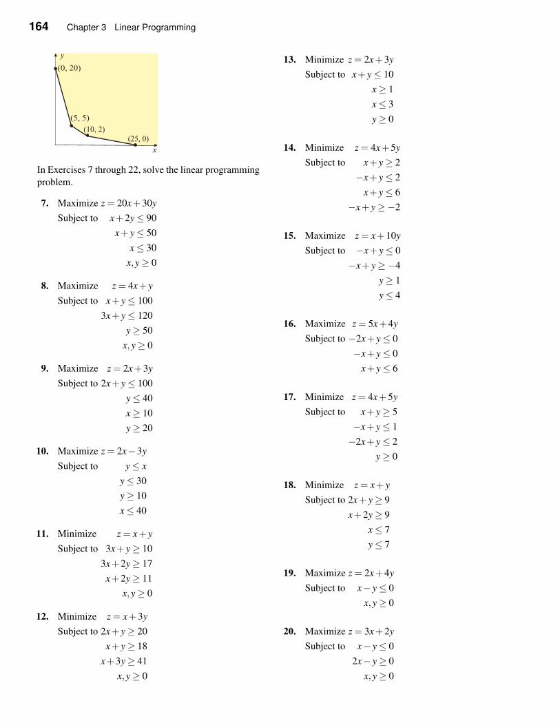
164 Chapter 3 Linear Programming
In Exercises 7 through 22, solve the linear programming
problem.
7. Maximize z = 20x+30y
Subject to x+2y≤ 90
x+ y≤ 50
x≤ 30
x,y≥ 0
8. Maximize z = 4x+ y
Subject to x+ y≤ 100
3x+ y≤ 120
y≥ 50
x,y≥ 0
9. Maximize z = 2x+3y
Subject to 2x+ y≤ 100
y≤ 40
x≥ 10
y≥ 20
10. Maximize z = 2x−3y
Subject to y≤ x
y≤ 30
y≥ 10
x≤ 40
11. Minimize z = x+ y
Subject to 3x+ y≥ 10
3x+2y≥ 17
x+2y≥ 11
x,y≥ 0
12. Minimize z = x+3y
Subject to 2x+ y≥ 20
x+ y≥ 18
x+3y≥ 41
x,y≥ 0
13. Minimize z = 2x+3y
Subject to x+ y≤ 10
x≥ 1
x≤ 3
y≥ 0
14. Minimize z = 4x+5y
Subject to x+ y≥ 2
−x+ y≤ 2
x+ y≤ 6
−x+ y≥−2
15. Maximize z = x+10y
Subject to −x+ y≤ 0
−x+ y≥−4
y≥ 1
y≤ 4
16. Maximize z = 5x+4y
Subject to −2x+ y≤ 0
−x+ y≤ 0
x+ y≤ 6
17. Minimize z = 4x+5y
Subject to x+ y≥ 5
−x+ y≤ 1
−2x+ y≤ 2
y≥ 0
18. Minimize z = x+ y
Subject to 2x+ y≥ 9
x+2y≥ 9
x≤ 7
y≤ 7
19. Maximize z = 2x+4y
Subject to x− y≤ 0
x,y≥ 0
20. Maximize z = 3x+2y
Subject to x− y≤ 0
2x− y≥ 0
x,y≥ 0
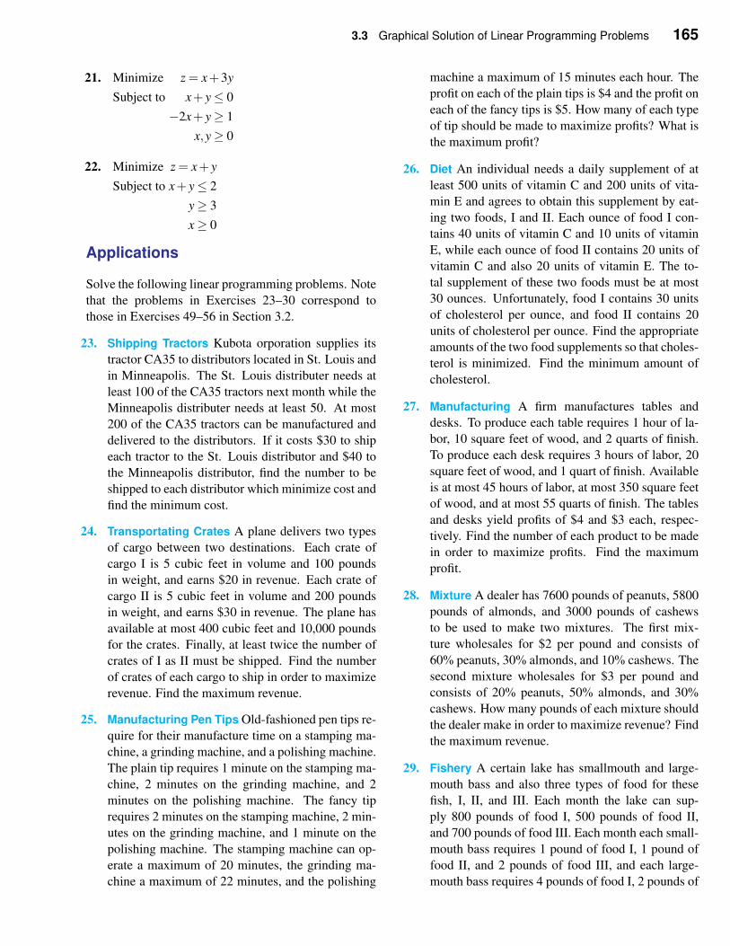
3.3 Graphical Solution of Linear Programming Problems 165
21. Minimize z = x+3y
Subject to x+ y≤ 0
−2x+ y≥ 1
x,y≥ 0
22. Minimize z = x+ y
Subject to x+ y≤ 2
y≥ 3
x≥ 0
Applications
Solve the following linear programming problems. Note
that the problems in Exercises 23–30 correspond to
those in Exercises 49–56 in Section 3.2.
23. Shipping Tractors Kubota orporation supplies its
tractor CA35 to distributors located in St. Louis and
in Minneapolis. The St. Louis distributer needs at
least 100 of the CA35 tractors next month while the
Minneapolis distributer needs at least 50. At most
200 of the CA35 tractors can be manufactured and
delivered to the distributors. If it costs $30 to ship
each tractor to the St. Louis distributor and $40 to
the Minneapolis distributor, find the number to be
shipped to each distributor which minimize cost and
find the minimum cost.
24. Transportating Crates A plane delivers two types
of cargo between two destinations. Each crate of
cargo I is 5 cubic feet in volume and 100 pounds
in weight, and earns $20 in revenue. Each crate of
cargo II is 5 cubic feet in volume and 200 pounds
in weight, and earns $30 in revenue. The plane has
available at most 400 cubic feet and 10,000 pounds
for the crates. Finally, at least twice the number of
crates of I as II must be shipped. Find the number
of crates of each cargo to ship in order to maximize
revenue. Find the maximum revenue.
25. Manufacturing Pen Tips Old-fashioned pen tips re-
quire for their manufacture time on a stamping ma-
chine, a grinding machine, and a polishing machine.
The plain tip requires 1 minute on the stamping ma-
chine, 2 minutes on the grinding machine, and 2
minutes on the polishing machine. The fancy tip
requires 2 minutes on the stamping machine, 2 min-
utes on the grinding machine, and 1 minute on the
polishing machine. The stamping machine can op-
erate a maximum of 20 minutes, the grinding ma-
chine a maximum of 22 minutes, and the polishing
machine a maximum of 15 minutes each hour. The
profit on each of the plain tips is $4 and the profit on
each of the fancy tips is $5. How many of each type
of tip should be made to maximize profits? What is
the maximum profit?
26. Diet An individual needs a daily supplement of at
least 500 units of vitamin C and 200 units of vita-
min E and agrees to obtain this supplement by eat-
ing two foods, I and II. Each ounce of food I con-
tains 40 units of vitamin C and 10 units of vitamin
E, while each ounce of food II contains 20 units of
vitamin C and also 20 units of vitamin E. The to-
tal supplement of these two foods must be at most
30 ounces. Unfortunately, food I contains 30 units
of cholesterol per ounce, and food II contains 20
units of cholesterol per ounce. Find the appropriate
amounts of the two food supplements so that choles-
terol is minimized. Find the minimum amount of
cholesterol.
27. Manufacturing A firm manufactures tables and
desks. To produce each table requires 1 hour of la-
bor, 10 square feet of wood, and 2 quarts of finish.
To produce each desk requires 3 hours of labor, 20
square feet of wood, and 1 quart of finish. Available
is at most 45 hours of labor, at most 350 square feet
of wood, and at most 55 quarts of finish. The tables
and desks yield profits of $4 and $3 each, respec-
tively. Find the number of each product to be made
in order to maximize profits. Find the maximum
profit.
28. Mixture A dealer has 7600 pounds of peanuts, 5800
pounds of almonds, and 3000 pounds of cashews
to be used to make two mixtures. The first mix-
ture wholesales for $2 per pound and consists of
60% peanuts, 30% almonds, and 10% cashews. The
second mixture wholesales for $3 per pound and
consists of 20% peanuts, 50% almonds, and 30%
cashews. How many pounds of each mixture should
the dealer make in order to maximize revenue? Find
the maximum revenue.
29. Fishery A certain lake has smallmouth and large-
mouth bass and also three types of food for these
fish, I, II, and III. Each month the lake can sup-
ply 800 pounds of food I, 500 pounds of food II,
and 700 pounds of food III. Each month each small-
mouth bass requires 1 pound of food I, 1 pound of
food II, and 2 pounds of food III, and each large-
mouth bass requires 4 pounds of food I, 2 pounds of
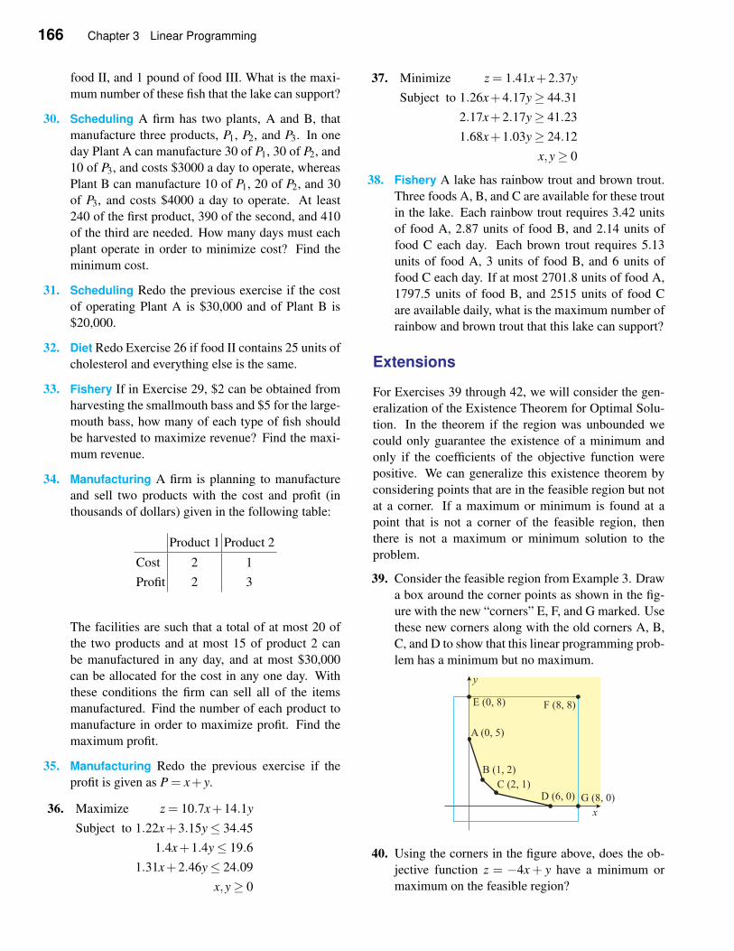
166 Chapter 3 Linear Programming
food II, and 1 pound of food III. What is the maxi-
mum number of these fish that the lake can support?
30. Scheduling A firm has two plants, A and B, that
manufacture three products, P1, P2, and P3. In one
day Plant A can manufacture 30 of P1, 30 of P2, and
10 of P3, and costs $3000 a day to operate, whereas
Plant B can manufacture 10 of P1, 20 of P2, and 30
of P3, and costs $4000 a day to operate. At least
240 of the first product, 390 of the second, and 410
of the third are needed. How many days must each
plant operate in order to minimize cost? Find the
minimum cost.
31. Scheduling Redo the previous exercise if the cost
of operating Plant A is $30,000 and of Plant B is
$20,000.
32. Diet Redo Exercise 26 if food II contains 25 units of
cholesterol and everything else is the same.
33. Fishery If in Exercise 29, $2 can be obtained from
harvesting the smallmouth bass and $5 for the large-
mouth bass, how many of each type of fish should
be harvested to maximize revenue? Find the maxi-
mum revenue.
34. Manufacturing A firm is planning to manufacture
and sell two products with the cost and profit (in
thousands of dollars) given in the following table:
Product 1 Product 2
Cost 2 1
Profit 2 3
The facilities are such that a total of at most 20 of
the two products and at most 15 of product 2 can
be manufactured in any day, and at most $30,000
can be allocated for the cost in any one day. With
these conditions the firm can sell all of the items
manufactured. Find the number of each product to
manufacture in order to maximize profit. Find the
maximum profit.
35. Manufacturing Redo the previous exercise if the
profit is given as P = x+ y.
36. Maximize z = 10.7x+14.1y
Subject to 1.22x+3.15y≤ 34.45
1.4x+1.4y≤ 19.6
1.31x+2.46y≤ 24.09
x,y≥ 0
37. Minimize z = 1.41x+2.37y
Subject to 1.26x+4.17y≥ 44.31
2.17x+2.17y≥ 41.23
1.68x+1.03y≥ 24.12
x,y≥ 0
38. Fishery A lake has rainbow trout and brown trout.
Three foods A, B, and C are available for these trout
in the lake. Each rainbow trout requires 3.42 units
of food A, 2.87 units of food B, and 2.14 units of
food C each day. Each brown trout requires 5.13
units of food A, 3 units of food B, and 6 units of
food C each day. If at most 2701.8 units of food A,
1797.5 units of food B, and 2515 units of food C
are available daily, what is the maximum number of
rainbow and brown trout that this lake can support?
Extensions
For Exercises 39 through 42, we will consider the gen-
eralization of the Existence Theorem for Optimal Solu-
tion. In the theorem if the region was unbounded we
could only guarantee the existence of a minimum and
only if the coefficients of the objective function were
positive. We can generalize this existence theorem by
considering points that are in the feasible region but not
at a corner. If a maximum or minimum is found at a
point that is not a corner of the feasible region, then
there is not a maximum or minimum solution to the
problem.
39. Consider the feasible region from Example 3. Draw
a box around the corner points as shown in the fig-
ure with the new “corners” E, F, and G marked. Use
these new corners along with the old corners A, B,
C, and D to show that this linear programming prob-
lem has a minimum but no maximum.
40. Using the corners in the figure above, does the ob-
jective function z = −4x + y have a minimum or
maximum on the feasible region?
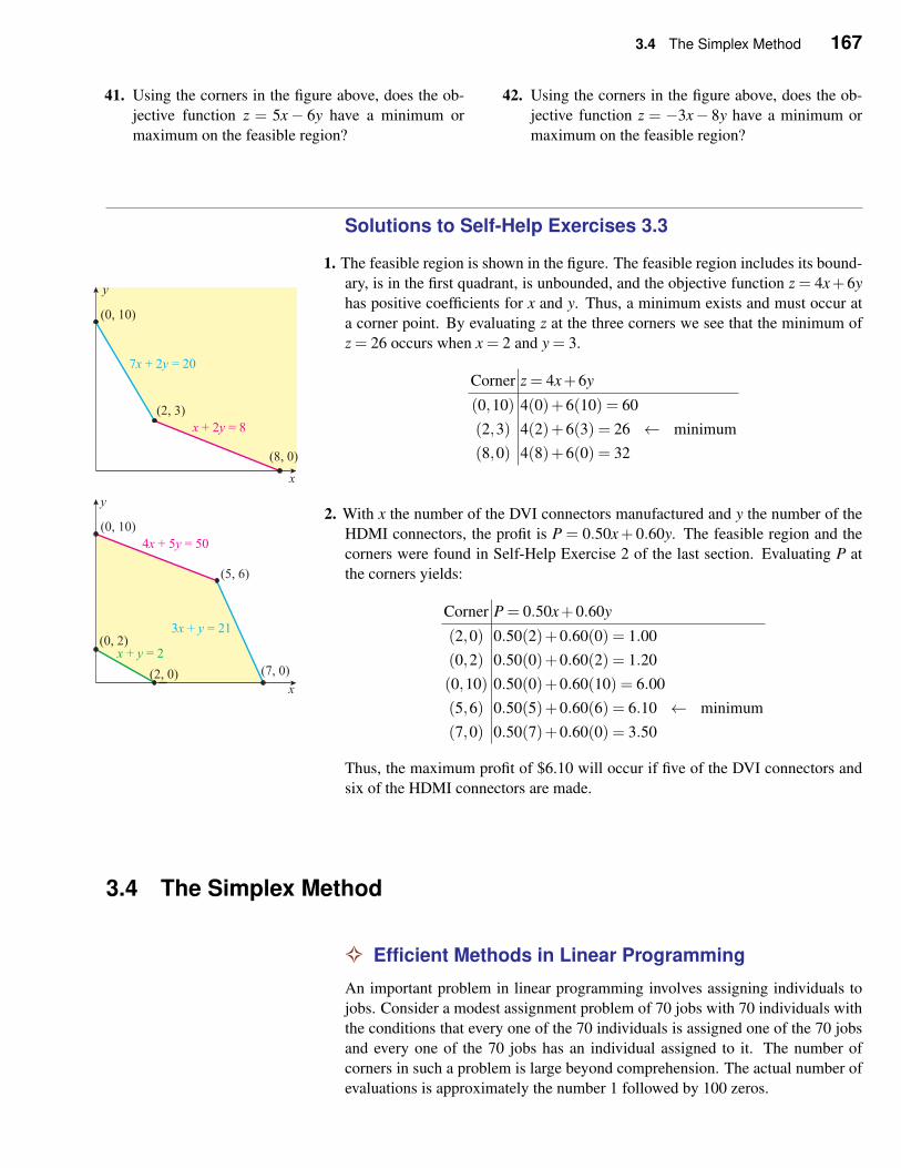
3.4 The Simplex Method 167
41. Using the corners in the figure above, does the ob-
jective function z = 5x− 6y have a minimum or
maximum on the feasible region?
42. Using the corners in the figure above, does the ob-
jective function z = −3x− 8y have a minimum or
maximum on the feasible region?
Solutions to Self-Help Exercises 3.3
1. The feasible region is shown in the figure. The feasible region includes its bound-
ary, is in the first quadrant, is unbounded, and the objective function z = 4x+6y
has positive coefficients for x and y. Thus, a minimum exists and must occur at
a corner point. By evaluating z at the three corners we see that the minimum of
z = 26 occurs when x = 2 and y = 3.
Corner z = 4x+6y
(0,10) 4(0)+6(10) = 60
(2,3) 4(2)+6(3) = 26 ← minimum
(8,0) 4(8)+6(0) = 32
2. With x the number of the DVI connectors manufactured and y the number of the
HDMI connectors, the profit is P = 0.50x+ 0.60y. The feasible region and the
corners were found in Self-Help Exercise 2 of the last section. Evaluating P at
the corners yields:
Corner P = 0.50x+0.60y
(2,0) 0.50(2)+0.60(0) = 1.00
(0,2) 0.50(0)+0.60(2) = 1.20
(0,10) 0.50(0)+0.60(10) = 6.00
(5,6) 0.50(5)+0.60(6) = 6.10 ← minimum
(7,0) 0.50(7)+0.60(0) = 3.50
Thus, the maximum profit of $6.10 will occur if five of the DVI connectors and
six of the HDMI connectors are made.
3.4 The Simplex Method
✧ Efficient Methods in Linear Programming
An important problem in linear programming involves assigning individuals to
jobs. Consider a modest assignment problem of 70 jobs with 70 individuals with
the conditions that every one of the 70 individuals is assigned one of the 70 jobs
and every one of the 70 jobs has an individual assigned to it. The number of
corners in such a problem is large beyond comprehension. The actual number of
evaluations is approximately the number 1 followed by 100 zeros.
168 Chapter 3 Linear Programming
It is clear that for practical problems an efficient method is needed to find the
maximum or the minimum of the objective function. George Dantzig, father of
linear programming, discovered an efficient method in 1947 to find the solution
by looking at a very modest number of corners. This method, called the simplex
method, is considered in this chapter. The simplex method can solve impor-
tant practical linear programming problems in reasonable time using computers
available today.
In Section 3.3 we used the Method of Corners to find where the optimal value
of the objective function occurred. To find the corners of the feasible region we
graphed the system of linear inequalities. This limited us to problems with only
two variables. What we need now is an algebraic method of finding the corners
for a problem with any number of variables. To do this we must convert our
system of linear inequalities to a system of linear equations. This will require
us to introduce additional variables, but we will be able to find the corners and
evaluate the objective function to find the optimal value.
The algebraic method is called the simplex method and it can be readily pro-
grammed for use on computers. The method systematically and efficiently moves
from one corner point of the feasible region to an adjacent corner point, always
improving the objective function (or at least not making it worse) until the corner
is found that maximizes the objective function.
✧ Standard Maximization Problems
In this section the simplex method is applied only to the so-called standard max-
imization problems. We begin by defining what a standard maximization prob-
lem is:
Standard Maximization Problem
A linear programming problem is said to be a standard maximization
problem if the following are satisfied.
1. The decision variables are constrained to be nonnegative. This is
called the nonnegative condition.
2. All of the problem constraint inequalities are ≤ a nonnegative con-
stant.
3. The objective function is to be maximized.
EXAMPLE 1 A Standard Maximization Problem Show that the problem of
the wooden-boat manufacturer of Section 3.3 is a standard maximization prob-
lem.
Solution If x1 is the number of dinghies produced, x2 the number of skiffs, and
P is the profit, then recall that the linear programming problem was
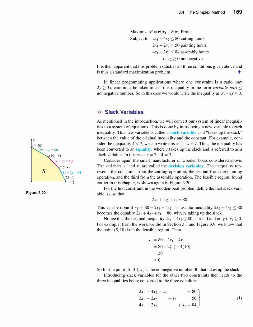
3.4 The Simplex Method 169
Maximize P = 60x1 +80x2 Profit
Subject to 2x1 +4x2 ≤ 80 cutting hours
2x1 +2x2 ≤ 50 painting hours
4x1 +2x2 ≤ 84 assembly hours
x1,x2 ≥ 0 nonnegative
It is then apparent that this problem satisfies all three conditions given above and
is thus a standard maximization problem. ✦
In linear programming applications where one constraint is a ratio, say
2y ≥ 3x, care must be taken to cast this inequality in the form variable part ≤nonnegative number. So in this case we would write the inequality as 3x−2y≤ 0.
✧ Slack Variables
As mentioned in the introduction, we will convert our system of linear inequali-
ties to a system of equations. This is done by introducing a new variable to each
inequality. This new variable is called a slack variable as it “takes up the slack”
between the value of the original inequality and the constant. For example, con-
sider the inequality 4 < 7, we can write this as 4+ s = 7. Thus, the inequality has
been converted to an equality, where s takes up the slack and is referred to as a
slack variable. In this case, s = 7−4 = 3.
Consider again the small manufacturer of wooden boats considered above.
The variables x1 and x2 are called the decision variables. The inequality rep-
resents the constraint from the cutting operation, the second from the painting
operation, and the third from the assembly operation. The feasible region, found
earlier in this chapter, is shown again in Figure 3.20.
Figure 3.20For the first constraint in the wooden-boat problem define the first slack vari-
able, s1, so that
2x1 +4x2 + s1 = 80
This can be done if s1 = 80− 2x1− 4x2. Thus, the inequality 2x1 + 4x2 ≤ 80
becomes the equality 2x1 +4x2 + s1 = 80, with s1 taking up the slack.
Notice that the original inequality 2x1+4x2 ≤ 80 is true if and only if s1 ≥ 0.
For example, from the work we did in Section 3.3 and Figure 3.9, we know that
the point (5,10) is in the feasible region. Then
s1 = 80−2x1−4x2
= 80−2(5)−4(10)
= 30
≥ 0
So for the point (5,10), s1 is the nonnegative number 30 that takes up the slack.
Introducing slack variables for the other two constraints then leads to the
three inequalities being converted to the three equalities:
2x1 + 4x2 + s1 = 80
2x1 + 2x2 + s2 = 50
4x1 + 2x2 + s3 = 84
(1)
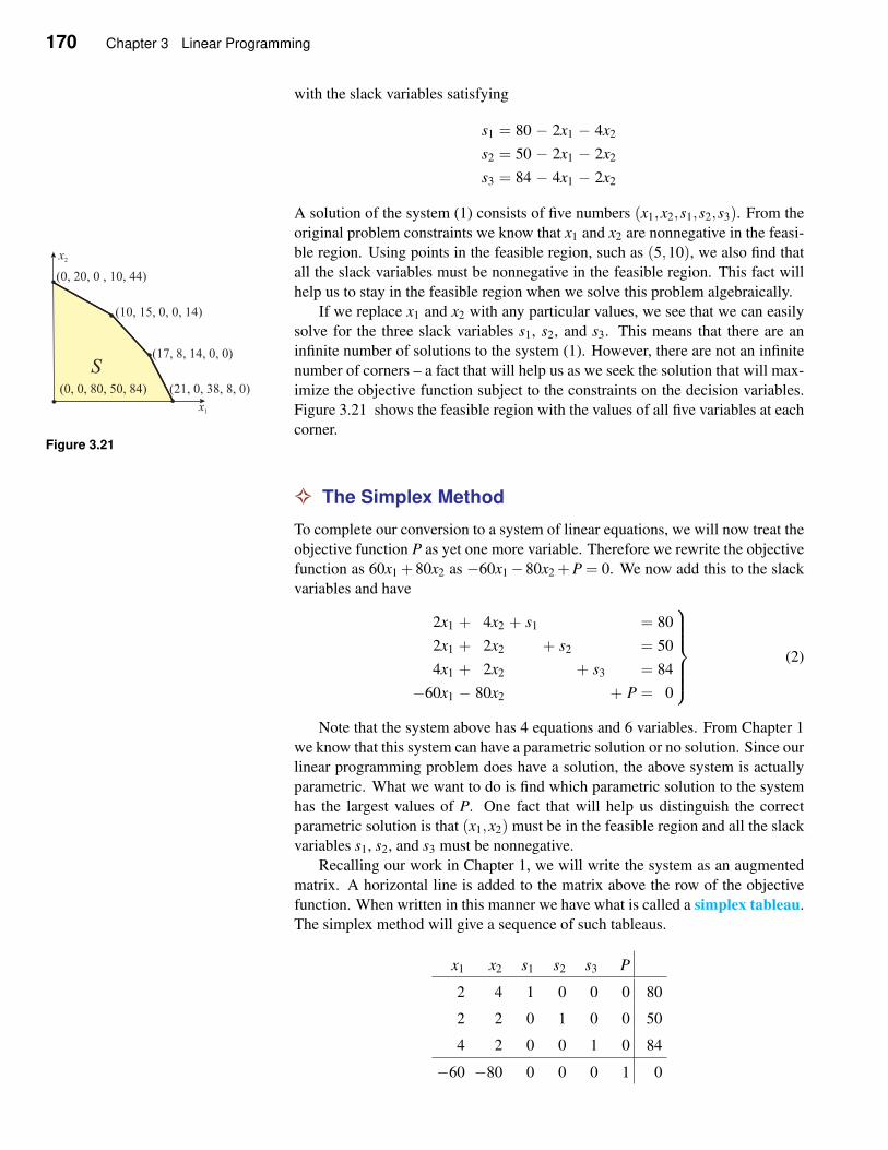
170 Chapter 3 Linear Programming
with the slack variables satisfying
s1 = 80 − 2x1 − 4x2
s2 = 50 − 2x1 − 2x2
s3 = 84 − 4x1 − 2x2
A solution of the system (1) consists of five numbers (x1,x2,s1,s2,s3). From the
original problem constraints we know that x1 and x2 are nonnegative in the feasi-
ble region. Using points in the feasible region, such as (5,10), we also find that
all the slack variables must be nonnegative in the feasible region. This fact will
help us to stay in the feasible region when we solve this problem algebraically.
If we replace x1 and x2 with any particular values, we see that we can easily
solve for the three slack variables s1, s2, and s3. This means that there are an
infinite number of solutions to the system (1). However, there are not an infinite
number of corners – a fact that will help us as we seek the solution that will max-
imize the objective function subject to the constraints on the decision variables.
Figure 3.21 shows the feasible region with the values of all five variables at each
Figure 3.21corner.
✧ The Simplex Method
To complete our conversion to a system of linear equations, we will now treat the
objective function P as yet one more variable. Therefore we rewrite the objective
function as 60x1 + 80x2 as −60x1− 80x2 +P = 0. We now add this to the slack
variables and have
2x1 + 4x2 + s1 = 80
2x1 + 2x2 + s2 = 50
4x1 + 2x2 + s3 = 84
−60x1 − 80x2 + P = 0
(2)
Note that the system above has 4 equations and 6 variables. From Chapter 1
we know that this system can have a parametric solution or no solution. Since our
linear programming problem does have a solution, the above system is actually
parametric. What we want to do is find which parametric solution to the system
has the largest values of P. One fact that will help us distinguish the correct
parametric solution is that (x1,x2) must be in the feasible region and all the slack
variables s1, s2, and s3 must be nonnegative.
Recalling our work in Chapter 1, we will write the system as an augmented
matrix. A horizontal line is added to the matrix above the row of the objective
function. When written in this manner we have what is called a simplex tableau.
The simplex method will give a sequence of such tableaus.
x1 x2 s1 s2 s3 P
2 4 1 0 0 0 80
2 2 0 1 0 0 50
4 2 0 0 1 0 84
−60 −80 0 0 0 1 0
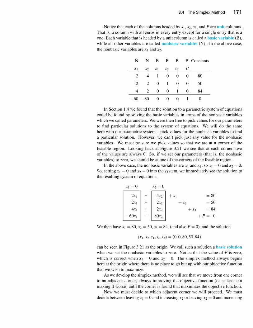
3.4 The Simplex Method 171
Notice that each of the columns headed by s1, s2, s3, and P are unit columns.
That is, a column with all zeros in every entry except for a single entry that is a
one. Each variable that is headed by a unit column is called a basic variable (B),
while all other variables are called nonbasic variables (N) . In the above case,
the nonbasic variables are x1 and x2.
N N B B B B Constants
x1 x2 s1 s2 s3 P
2 4 1 0 0 0 80
2 2 0 1 0 0 50
4 2 0 0 1 0 84
−60 −80 0 0 0 1 0
In Section 1.4 we found that the solution to a parametric system of equations
could be found by solving the basic variables in terms of the nonbasic variables
which we called parameters. We were then free to pick values for our parameters
to find particular solutions to the system of equations. We will do the same
here with our parametric system – pick values for the nonbasic variables to find
a particular solution. However, we can’t pick just any value for the nonbasic
variables. We must be sure we pick values so that we are at a corner of the
feasible region. Looking back at Figure 3.21 we see that at each corner, two
of the values are always 0. So, if we set our parameters (that is, the nonbasic
variables) to zero, we should be at one of the corners of the feasible region.
In the above case, the nonbasic variables are x1 and x2, so x1 = 0 and x2 = 0.
So, setting x1 = 0 and x2 = 0 into the system, we immediately see the solution to
the resulting system of equations.
x1 = 0 x2 = 0
2x1
2x1
4x1
−60x1
+
+
+
−
4x2
2x2
2x2
80x2
+ s1 = 80
+ s2 = 50
+ s3 = 84
+ P = 0
We then have s1 = 80, s2 = 50, s3 = 84, (and also P = 0), and the solution
(x1,x2,s1,s2,s3) = (0,0,80,50,84)
can be seen in Figure 3.21 as the origin. We call such a solution a basic solution
when we set the nonbasic variables to zero. Notice that the value of P is zero,
which is correct when x1 = 0 and x2 = 0. The simplex method always begins
here at the origin where there is no place to go but up with our objective function
that we wish to maximize.
As we develop the simplex method, we will see that we move from one corner
to an adjacent corner, always improving the objective function (or at least not
making it worse) until the corner is found that maximizes the objective function.
Now we must decide to which adjacent corner we will proceed. We must
decide between leaving x1 = 0 and increasing x2 or leaving x2 = 0 and increasing
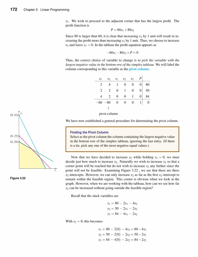
172 Chapter 3 Linear Programming
x1. We wish to proceed to the adjacent corner that has the largest profit. The
profit function is
P = 60x1 +80x2
Since 80 is larger than 60, it is clear that increasing x2 by 1 unit will result in in-
creasing the profit more than increasing x1 by 1 unit. Thus, we choose to increase
x2 and leave x1 = 0. In the tableau the profit equation appears as
−60x1−80x2 +P = 0
Thus, the correct choice of variable to change is to pick the variable with the
largest negative value in the bottom row of the simplex tableau. We will label the
column corresponding to this variable as the pivot column.
x1 x2 s1 s2 s3 P
2 4 1 0 0 0 80
2 2 0 1 0 0 50
4 2 0 0 1 0 84
−60 −80 0 0 0 1 0
↑pivot column
We have now established a general procedure for determining the pivot column.
Finding the Pivot Column
Select as the pivot column the column containing the largest negative value
in the bottom row of the simplex tableau, ignoring the last entry. (If there
is a tie, pick any one of the most negative equal values.)
Now that we have decided to increase x2 while holding x1 = 0, we must
decide just how much to increase x2. Naturally we wish to increase x2 so that a
corner point will be reached but do not wish to increase x2 any further since the
point will not be feasible. Examining Figure 3.22 , we see that there are three
Figure 3.22x2-intercepts. However, we can only increase x2 as far as the first x2-intercept to
remain within the feasible region. This corner is obvious when we look at the
graph. However, when we are working with the tableau, how can we see how far
x2 can be increased without going outside the feasible region?
Recall that the slack variables are
s1 = 80 − 2x1 − 4x2
s2 = 50 − 2x1 − 2x2
s3 = 84 − 4x1 − 2x2
With x1 = 0, this becomes
s1 = 80 − 2(0) − 4x2 = 80−4x2
s2 = 50 − 2(0) − 2x2 = 50−2x2
s3 = 84 − 4(0) − 2x2 = 84−2x2
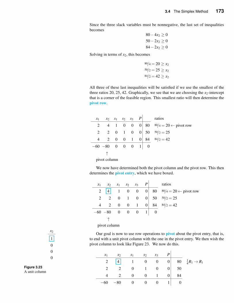
3.4 The Simplex Method 173
Since the three slack variables must be nonnegative, the last set of inequalities
becomes80−4x2 ≥ 0
50−2x2 ≥ 0
84−2x2 ≥ 0
Solving in terms of x2, this becomes
80/4 = 20 ≥ x2
50/2 = 25 ≥ x2
84/2 = 42 ≥ x2
All three of these last inequalities will be satisfied if we use the smallest of the
three ratios 20, 25, 42. Graphically, we see that we are choosing the x2-intercept
that is a corner of the feasible region. This smallest ratio will then determine the
pivot row.
x1 x2 s1 s2 s3 P ratios
2 4 1 0 0 0 80 80/4 = 20← pivot row
2 2 0 1 0 0 50 50/2 = 25
4 2 0 0 1 0 84 84/2 = 42
−60 −80 0 0 0 1 0
↑pivot column
We now have determined both the pivot column and the pivot row. This then
determines the pivot entry, which we have boxed.
x1 x2 s1 s2 s3 P ratios
2 4 1 0 0 0 80 80/4 = 20← pivot row
2 2 0 1 0 0 50 50/2 = 25
4 2 0 0 1 0 84 84/2 = 42
−60 −80 0 0 0 1 0
↑pivot column
Our goal is now to use row operations to pivot about the pivot entry, that is,
to end with a unit pivot column with the one in the pivot entry. We then wish the
pivot column to look like Figure 23. We now do this.
x2
1
0
0
0
Figure 3.23
A unit column
x1 x2 s1 s2 s3 P
2 4 1 0 0 0 80 14 R1→ R1
2 2 0 1 0 0 50
4 2 0 0 1 0 84
−60 −80 0 0 0 1 0
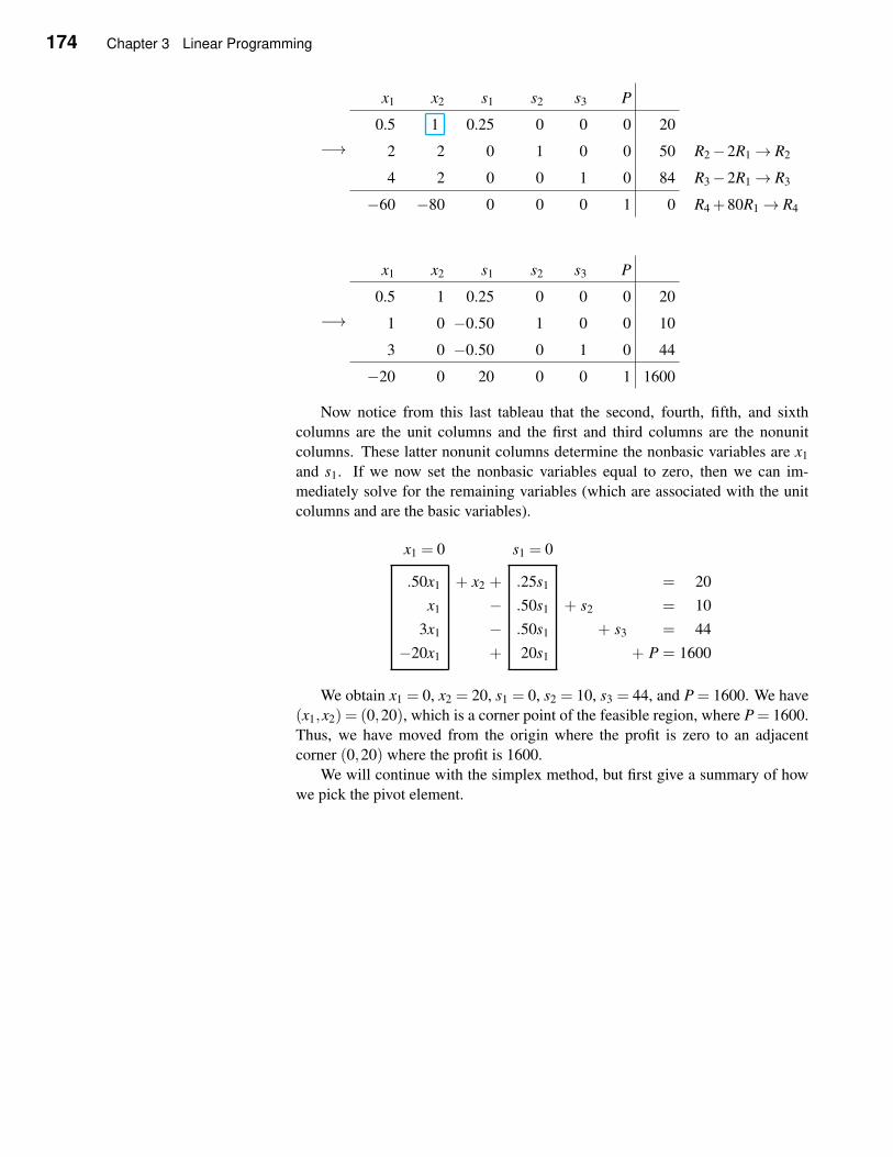
174 Chapter 3 Linear Programming
−→
x1 x2 s1 s2 s3 P
0.5 1 0.25 0 0 0 20
2 2 0 1 0 0 50 R2−2R1→ R2
4 2 0 0 1 0 84 R3−2R1→ R3
−60 −80 0 0 0 1 0 R4 +80R1→ R4
−→
x1 x2 s1 s2 s3 P
0.5 1 0.25 0 0 0 20
1 0 −0.50 1 0 0 10
3 0 −0.50 0 1 0 44
−20 0 20 0 0 1 1600
Now notice from this last tableau that the second, fourth, fifth, and sixth
columns are the unit columns and the first and third columns are the nonunit
columns. These latter nonunit columns determine the nonbasic variables are x1
and s1. If we now set the nonbasic variables equal to zero, then we can im-
mediately solve for the remaining variables (which are associated with the unit
columns and are the basic variables).
x1 = 0 s1 = 0
.50x1
x1
3x1
−20x1
+ x2 +
−−+
.25s1
.50s1
.50s1
20s1
= 20
+ s2 = 10
+ s3 = 44
+ P = 1600
We obtain x1 = 0, x2 = 20, s1 = 0, s2 = 10, s3 = 44, and P = 1600. We have
(x1,x2) = (0,20), which is a corner point of the feasible region, where P = 1600.
Thus, we have moved from the origin where the profit is zero to an adjacent
corner (0,20) where the profit is 1600.
We will continue with the simplex method, but first give a summary of how
we pick the pivot element.
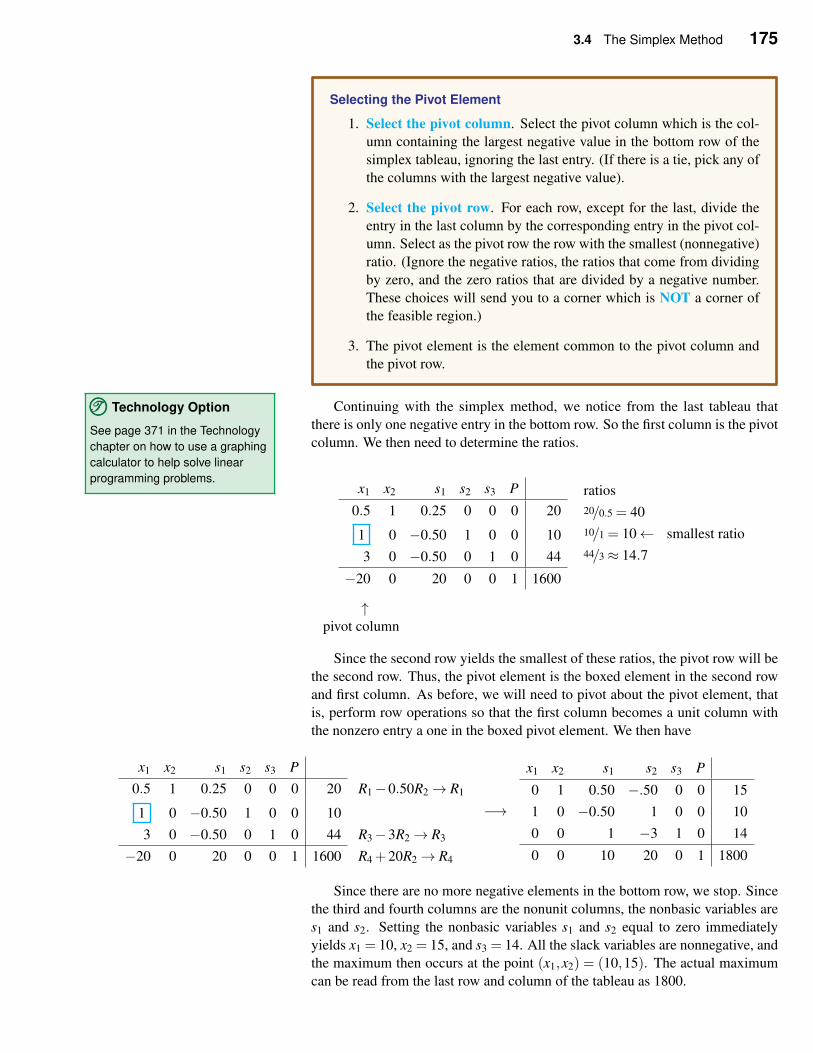
3.4 The Simplex Method 175
Selecting the Pivot Element
1. Select the pivot column. Select the pivot column which is the col-
umn containing the largest negative value in the bottom row of the
simplex tableau, ignoring the last entry. (If there is a tie, pick any of
the columns with the largest negative value).
2. Select the pivot row. For each row, except for the last, divide the
entry in the last column by the corresponding entry in the pivot col-
umn. Select as the pivot row the row with the smallest (nonnegative)
ratio. (Ignore the negative ratios, the ratios that come from dividing
by zero, and the zero ratios that are divided by a negative number.
These choices will send you to a corner which is NOT a corner of
the feasible region.)
3. The pivot element is the element common to the pivot column and
the pivot row.
Continuing with the simplex method, we notice from the last tableau that
there is only one negative entry in the bottom row. So the first column is the pivot
column. We then need to determine the ratios.
TTT©©© Technology Option
See page 371 in the Technology
chapter on how to use a graphing
calculator to help solve linear
programming problems.x1 x2 s1 s2 s3 P
0.5 1 0.25 0 0 0 20
1 0 −0.50 1 0 0 10
3 0 −0.50 0 1 0 44
−20 0 20 0 0 1 1600
ratios
20/0.5 = 40
10/1 = 10← smallest ratio
44/3≈ 14.7
↑pivot column
Since the second row yields the smallest of these ratios, the pivot row will be
the second row. Thus, the pivot element is the boxed element in the second row
and first column. As before, we will need to pivot about the pivot element, that
is, perform row operations so that the first column becomes a unit column with
the nonzero entry a one in the boxed pivot element. We then have
x1 x2 s1 s2 s3 P
0.5 1 0.25 0 0 0 20 R1−0.50R2→ R1
1 0 −0.50 1 0 0 10
3 0 −0.50 0 1 0 44 R3−3R2→ R3
−20 0 20 0 0 1 1600 R4 +20R2→ R4
−→
x1 x2 s1 s2 s3 P
0 1 0.50 −.50 0 0 15
1 0 −0.50 1 0 0 10
0 0 1 −3 1 0 14
0 0 10 20 0 1 1800
Since there are no more negative elements in the bottom row, we stop. Since
the third and fourth columns are the nonunit columns, the nonbasic variables are
s1 and s2. Setting the nonbasic variables s1 and s2 equal to zero immediately
yields x1 = 10, x2 = 15, and s3 = 14. All the slack variables are nonnegative, and
the maximum then occurs at the point (x1,x2) = (10,15). The actual maximum
can be read from the last row and column of the tableau as 1800.

176 Chapter 3 Linear Programming
Notice how the simplex method started at the corner (0,0), then moved to
(0,20), and then finally to (10,15), each time moving to an adjacent corner and
each time improving the maximum value of the objective function. Refer to
Figure 3.24.
Figure 3.24
We now summarize the steps in the simplex method.
The Simplex Method
1. Set up the initial simplex tableau in the following manner:
• Introduce a slack variable for each of the constraints and write
it as an equality.
• Rewrite the objective function in the form ...−P = 0.
• Put this system of linear equations in an augmented matrix with
the objective function as the bottom row.
2. Examine the entries in the bottom row of the augmented matrix. If
no negative entries remain, a solution has been found. Go to Step 4
to read the solution.
3. Select and perform the pivot:
• Find the most negative entry in the bottom row. This is the
pivot column. If there is a tie for the most negative entry, use
any of the columns with the most negative entry.
• Form the ratio q = a/b where a is the entry in the last column
of the matrix and b is the entry in the pivot column above the
horizontal line. Only find the ratio if b is greater than zero.
• Find the smallest nonnegative ratio. This is the pivot row.
• Pivot on the element that is in the pivot column and pivot row.
• Go to Step 2.
4. Read the solution:
• Identify the nonunit columns. These nonbasic variables are set
to zero.
• Read each row to find the values of the basic variables.
EXAMPLE 2 Using the Simplex Method
Maximize z = 3x1 +2x2
Subject to −x1 + x2 ≤ 2
2x1 + x2 ≤ 8
x1,x2 ≥ 0
Solution Introducing two slack variables and rewriting the objective function
yields
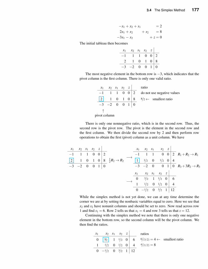
3.4 The Simplex Method 177
−x1 + x2 + s1 = 2
2x1 + x2 + s2 = 8
−3x1 − x2 + z = 0
The initial tableau then becomes
x1 x2 s1 s2 z
−1 1 1 0 0 2
2 1 0 1 0 8
−3 −2 0 0 1 0
The most negative element in the bottom row is −3, which indicates that the
pivot column is the first column. There is only one valid ratio.
x1 x2 s1 s2 z ratio
−1 1 1 0 0 2 do not use negative values
2 1 0 1 0 8 8/2← smallest ratio
−3 −2 0 0 1 0
↑pivot column
There is only one nonnegative ratio, which is in the second row. Thus, the
second row is the pivot row. The pivot is the element in the second row and
the first column. We then divide the second row by 2 and then perform row
operations to obtain the first (pivot) column as a unit column. We have
x1 x2 s1 s2 z
−1 1 1 0 0 2
2 1 0 1 0 8
−3 −2 0 0 1 0
12 R2→ R2
−→
x1 x2 s1 s2 z
−1 1 1 0 0 2 R1 +R2→ R1
1 1/2 0 1/2 0 4
−3 −2 0 0 1 0 R3 +3R2→ R3
−→
x1 x2 s1 s2 z
0 3/2 1 1/2 0 6
1 1/2 0 1/2 0 4
0 −1/2 0 3/2 1 12
While the simplex method is not yet done, we can at any time determine the
corner we are at by setting the nonbasic variables equal to zero. Here we see that
x2 and s2 have nonunit columns and should be set to zero. Now read across row
1 and find s1 = 6. Row 2 tells us that x1 = 4 and row 3 tells us that z = 12.
Continuing with the simplex method we note that there is only one negative
element in the bottom row, so the second column will be the pivot column. We
then find the ratios.
x1 x2 s1 s2 z
0 3/2 1 1/2 0 6
1 1/2 0 1/2 0 4
0 −1/2 0 3/2 1 12
ratios
6/(3/2) = 4← smallest ratio
4/(1/2) = 8
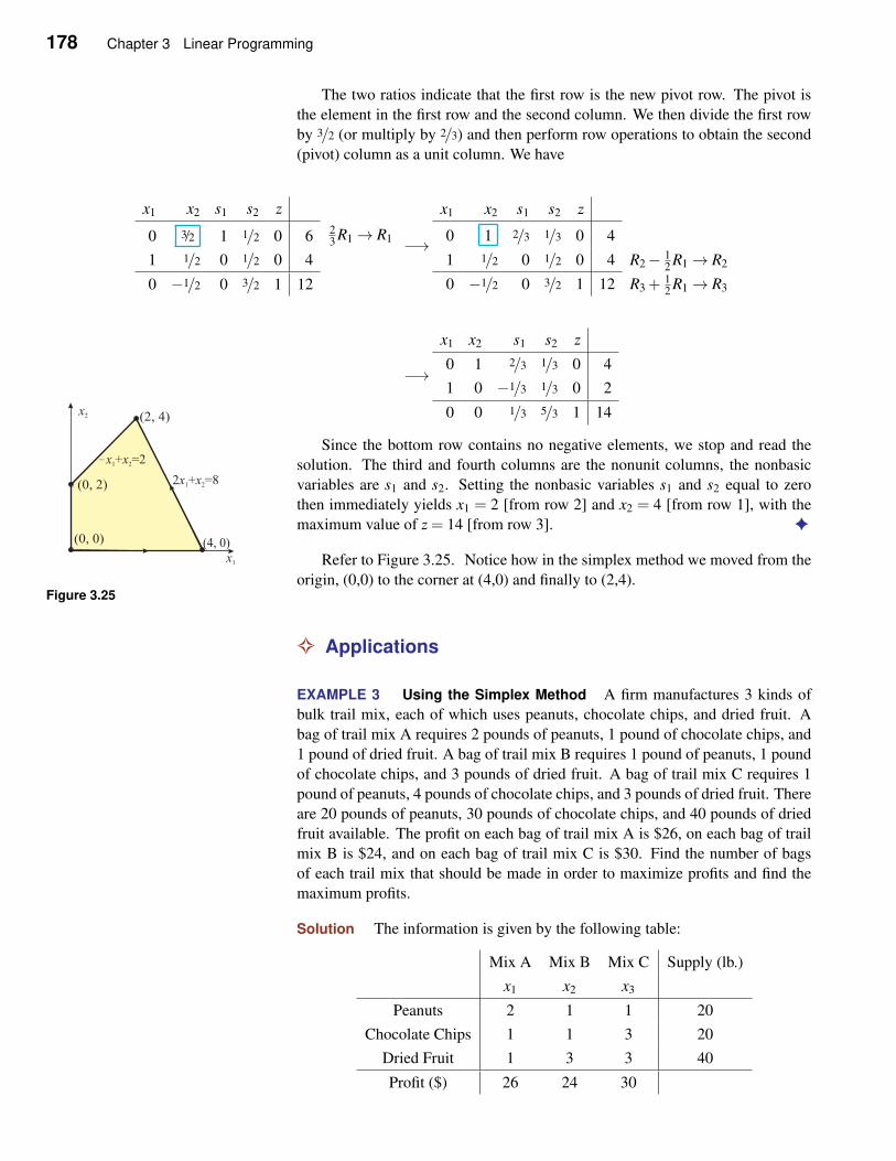
178 Chapter 3 Linear Programming
The two ratios indicate that the first row is the new pivot row. The pivot is
the element in the first row and the second column. We then divide the first row
by 3/2 (or multiply by 2/3) and then perform row operations to obtain the second
(pivot) column as a unit column. We have
x1 x2 s1 s2 z
0 3/2 1 1/2 0 6
1 1/2 0 1/2 0 4
0 −1/2 0 3/2 1 12
23 R1→ R1 −→
x1 x2 s1 s2 z
0 1 2/3 1/3 0 4
1 1/2 0 1/2 0 4 R2− 12 R1→ R2
0 −1/2 0 3/2 1 12 R3 +12 R1→ R3
−→
x1 x2 s1 s2 z
0 1 2/3 1/3 0 4
1 0 −1/3 1/3 0 2
0 0 1/3 5/3 1 14
Since the bottom row contains no negative elements, we stop and read the
solution. The third and fourth columns are the nonunit columns, the nonbasic
variables are s1 and s2. Setting the nonbasic variables s1 and s2 equal to zero
then immediately yields x1 = 2 [from row 2] and x2 = 4 [from row 1], with the
maximum value of z = 14 [from row 3]. ✦
Refer to Figure 3.25. Notice how in the simplex method we moved from the
Figure 3.25origin, (0,0) to the corner at (4,0) and finally to (2,4).
✧ Applications
EXAMPLE 3 Using the Simplex Method A firm manufactures 3 kinds of
bulk trail mix, each of which uses peanuts, chocolate chips, and dried fruit. A
bag of trail mix A requires 2 pounds of peanuts, 1 pound of chocolate chips, and
1 pound of dried fruit. A bag of trail mix B requires 1 pound of peanuts, 1 pound
of chocolate chips, and 3 pounds of dried fruit. A bag of trail mix C requires 1
pound of peanuts, 4 pounds of chocolate chips, and 3 pounds of dried fruit. There
are 20 pounds of peanuts, 30 pounds of chocolate chips, and 40 pounds of dried
fruit available. The profit on each bag of trail mix A is $26, on each bag of trail
mix B is $24, and on each bag of trail mix C is $30. Find the number of bags
of each trail mix that should be made in order to maximize profits and find the
maximum profits.
Solution The information is given by the following table:
Mix A Mix B Mix C Supply (lb.)
x1 x2 x3
Peanuts 2 1 1 20
Chocolate Chips 1 1 3 20
Dried Fruit 1 3 3 40
Profit ($) 26 24 30
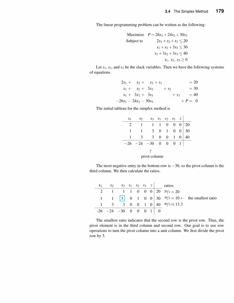
3.4 The Simplex Method 179
The linear programming problem can be written as the following:
Maximize P = 26x1 +24x2 +30x3
Subject to 2x1 + x2 + x3 ≤ 20
x1 + x2 +3x3 ≤ 30
x1 +3x2 +3x3 ≤ 40
x1, x2, x3 ≥ 0
Let s1, s2, and s3 be the slack variables. Then we have the following systems
of equations.
2x1 + x2 + x3 + s1 = 20
x1 + x2 + 3x3 + s2 = 30
x1 + 3x2 + 3x3 + s3 = 40
−26x1 − 24x2 − 30x3 + P = 0
The initial tableau for the simplex method is
x1 x2 x3 s1 s2 s3 z
2 1 1 1 0 0 0 20
1 1 3 0 1 0 0 30
1 3 3 0 0 1 0 40
−26 −24 −30 0 0 0 1
↑pivot column
The most negative entry in the bottom row is −30, so the pivot column is the
third column. We then calculate the ratios.
x1 x2 x3 s1 s2 s3 z
2 1 1 1 0 0 0 20
1 1 3 0 1 0 0 30
1 3 3 0 0 1 0 40
-26 −24 −30 0 0 0 1 0
ratios
20/1 = 20
30/3 = 10← the smallest ratio
40/3≈ 13.3
The smallest ratio indicates that the second row is the pivot row. Thus, the
pivot element is in the third column and second row. Our goal is to use row
operations to turn the pivot column into a unit column. We first divide the pivot
row by 3.
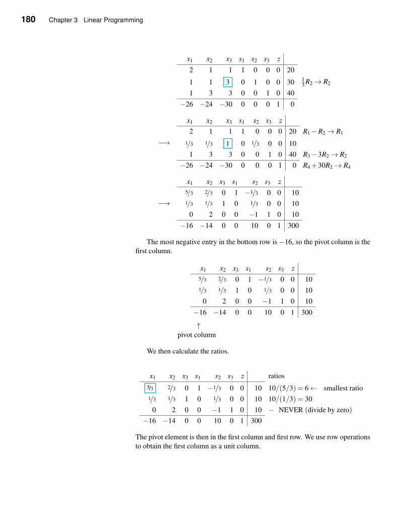
180 Chapter 3 Linear Programming
x1 x2 x3 s1 s2 s3 z
2 1 1 1 0 0 0 20
1 1 3 0 1 0 0 30
1 3 3 0 0 1 0 40
−26 −24 −30 0 0 0 1 0
13 R2→ R2
−→
x1 x2 x3 s1 s2 s3 z
2 1 1 1 0 0 0 20 R1−R2→ R1
1/3 1/3 1 0 1/3 0 0 10
1 3 3 0 0 1 0 40 R3−3R2→ R2
−26 −24 −30 0 0 0 1 0 R4 +30R2→ R4
−→
x1 x2 x3 s1 s2 s3 z
5/3 2/3 0 1 −1/3 0 0 10
1/3 1/3 1 0 1/3 0 0 10
0 2 0 0 −1 1 0 10
−16 −14 0 0 10 0 1 300
The most negative entry in the bottom row is −16, so the pivot column is the
first column.
x1 x2 x3 s1 s2 s3 z
5/3 2/3 0 1 −1/3 0 0 10
1/3 1/3 1 0 1/3 0 0 10
0 2 0 0 −1 1 0 10
−16 −14 0 0 10 0 1 300
↑pivot column
We then calculate the ratios.
x1 x2 x3 s1 s2 s3 z ratios
5/3 2/3 0 1 −1/3 0 0 10 10/(5/3) = 6← smallest ratio
1/3 1/3 1 0 1/3 0 0 10 10/(1/3) = 30
0 2 0 0 −1 1 0 10 − NEVER (divide by zero)
−16 −14 0 0 10 0 1 300
The pivot element is then in the first column and first row. We use row operations
to obtain the first column as a unit column.
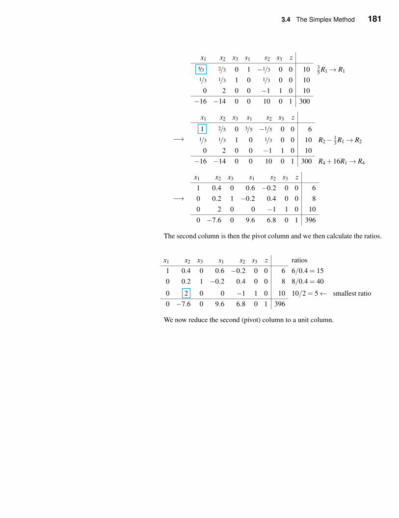
3.4 The Simplex Method 181
x1 x2 x3 s1 s2 s3 z
5/3 2/3 0 1 −1/3 0 0 10 35 R1→ R1
1/3 1/3 1 0 1/3 0 0 10
0 2 0 0 −1 1 0 10
−16 −14 0 0 10 0 1 300
−→
x1 x2 x3 s1 s2 s3 z
1 2/5 0 3/5 −1/5 0 0 6
1/3 1/3 1 0 1/3 0 0 10 R2− 13 R1→ R2
0 2 0 0 −1 1 0 10
−16 −14 0 0 10 0 1 300 R4 +16R1→ R4
−→
x1 x2 x3 s1 s2 s3 z
1 0.4 0 0.6 −0.2 0 0 6
0 0.2 1 −0.2 0.4 0 0 8
0 2 0 0 −1 1 0 10
0 −7.6 0 9.6 6.8 0 1 396
The second column is then the pivot column and we then calculate the ratios.
x1 x2 x3 s1 s2 s3 z ratios
1 0.4 0 0.6 −0.2 0 0 6 6/0.4 = 15
0 0.2 1 −0.2 0.4 0 0 8 8/0.4 = 40
0 2 0 0 −1 1 0 10 10/2 = 5← smallest ratio
0 −7.6 0 9.6 6.8 0 1 396
We now reduce the second (pivot) column to a unit column.
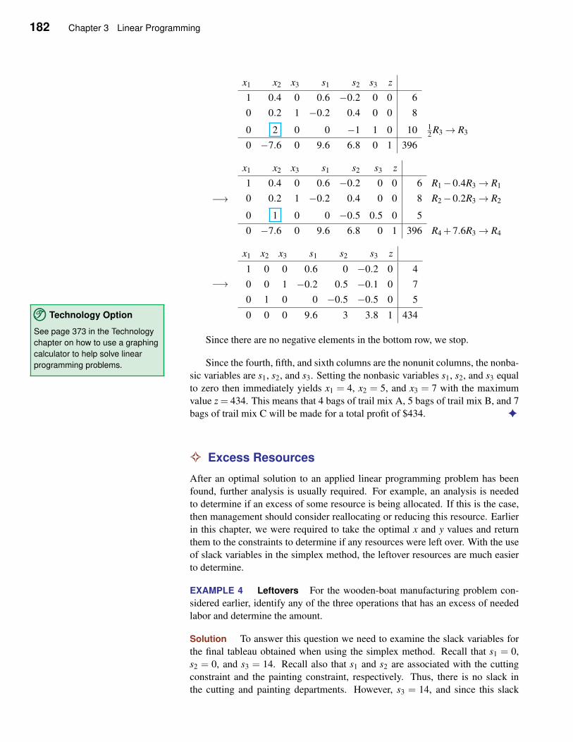
182 Chapter 3 Linear Programming
x1 x2 x3 s1 s2 s3 z
1 0.4 0 0.6 −0.2 0 0 6
0 0.2 1 −0.2 0.4 0 0 8
0 2 0 0 −1 1 0 10 12 R3→ R3
0 −7.6 0 9.6 6.8 0 1 396
−→
x1 x2 x3 s1 s2 s3 z
1 0.4 0 0.6 −0.2 0 0 6 R1−0.4R3→ R1
0 0.2 1 −0.2 0.4 0 0 8 R2−0.2R3→ R2
0 1 0 0 −0.5 0.5 0 5
0 −7.6 0 9.6 6.8 0 1 396 R4 +7.6R3→ R4
−→
x1 x2 x3 s1 s2 s3 z
1 0 0 0.6 0 −0.2 0 4
0 0 1 −0.2 0.5 −0.1 0 7
0 1 0 0 −0.5 −0.5 0 5
0 0 0 9.6 3 3.8 1 434
Since there are no negative elements in the bottom row, we stop.
TTT©©© Technology Option
See page 373 in the Technology
chapter on how to use a graphing
calculator to help solve linear
programming problems. Since the fourth, fifth, and sixth columns are the nonunit columns, the nonba-
sic variables are s1, s2, and s3. Setting the nonbasic variables s1, s2, and s3 equal
to zero then immediately yields x1 = 4, x2 = 5, and x3 = 7 with the maximum
value z = 434. This means that 4 bags of trail mix A, 5 bags of trail mix B, and 7
bags of trail mix C will be made for a total profit of $434. ✦
✧ Excess Resources
After an optimal solution to an applied linear programming problem has been
found, further analysis is usually required. For example, an analysis is needed
to determine if an excess of some resource is being allocated. If this is the case,
then management should consider reallocating or reducing this resource. Earlier
in this chapter, we were required to take the optimal x and y values and return
them to the constraints to determine if any resources were left over. With the use
of slack variables in the simplex method, the leftover resources are much easier
to determine.
EXAMPLE 4 Leftovers For the wooden-boat manufacturing problem con-
sidered earlier, identify any of the three operations that has an excess of needed
labor and determine the amount.
Solution To answer this question we need to examine the slack variables for
the final tableau obtained when using the simplex method. Recall that s1 = 0,
s2 = 0, and s3 = 14. Recall also that s1 and s2 are associated with the cutting
constraint and the painting constraint, respectively. Thus, there is no slack in
the cutting and painting departments. However, s3 = 14, and since this slack
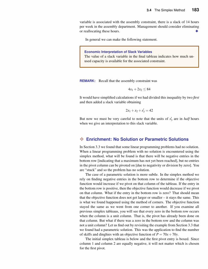
3.4 The Simplex Method 183
variable is associated with the assembly constraint, there is a slack of 14 hours
per week in the assembly department. Management should consider eliminating
or reallocating these hours. ✦
In general we can make the following statement.
Economic Interpretation of Slack Variables
The value of a slack variable in the final tableau indicates how much un-
used capacity is available for the associated constraint.
REMARK: Recall that the assembly constraint was
4x1 +2x2 ≤ 84
It would have simplified calculations if we had divided this inequality by two first
and then added a slack variable obtaining
2x1 + x2 + s′3 = 42
But now we must be very careful to note that the units of s′3 are in half hours
when we give an interpretation to this slack variable.
✧ Enrichment: No Solution or Parametric Solutions
In Section 3.3 we found that some linear programming problems had no solution.
When a linear programming problem with no solution is encountered using the
simplex method, what will be found is that there will be negative entries in the
bottom row [indicating that a maximum has not yet been reached], but no entries
in the pivot column can be pivoted on [due to negativity or division by zero]. You
are “stuck” and so the problem has no solution.
The case of a parametric solution is more subtle. In the simplex method we
rely on finding negative entries in the bottom row to determine if the objective
function would increase if we pivot on that column of the tableau. If the entry in
the bottom row is positive, then the objective function would decrease if we pivot
on that column. What if the entry in the bottom row is zero? That should mean
that the objective function does not get larger or smaller – it stays the same. This
is what we found happened using the method of corners. The objective function
stayed the same as we went from one corner to another. If you examine all
previous simplex tableaus, you will see that every zero in the bottom row occurs
when the column is a unit column. That is, the pivot has already been done on
that column. But what if there was a zero in the bottom row and the column was
not a unit column? Let us find out by revisiting the example from Section 3.3 that
we found had a parametric solution. This was the application to find the number
of skiffs and dinghies with an objective function of P = 70x+70y.
The initial simplex tableau is below and the first pivot entry is boxed. Since
column 1 and column 2 are equally negative, it will not matter which is chosen
for the first pivot.
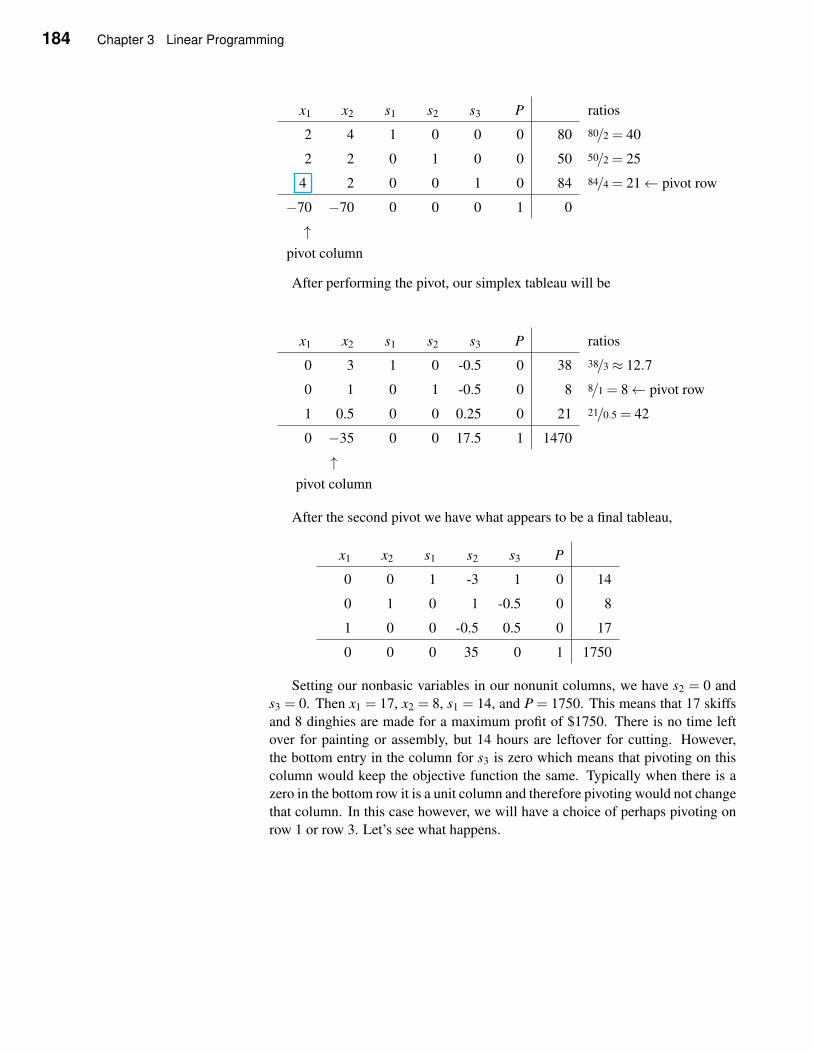
184 Chapter 3 Linear Programming
x1 x2 s1 s2 s3 P ratios
2 4 1 0 0 0 80 80/2 = 40
2 2 0 1 0 0 50 50/2 = 25
4 2 0 0 1 0 84 84/4 = 21← pivot row
−70 −70 0 0 0 1 0
↑pivot column
After performing the pivot, our simplex tableau will be
x1 x2 s1 s2 s3 P ratios
0 3 1 0 -0.5 0 38 38/3≈ 12.7
0 1 0 1 -0.5 0 8 8/1 = 8← pivot row
1 0.5 0 0 0.25 0 21 21/0.5 = 42
0 −35 0 0 17.5 1 1470
↑pivot column
After the second pivot we have what appears to be a final tableau,
x1 x2 s1 s2 s3 P
0 0 1 -3 1 0 14
0 1 0 1 -0.5 0 8
1 0 0 -0.5 0.5 0 17
0 0 0 35 0 1 1750
Setting our nonbasic variables in our nonunit columns, we have s2 = 0 and
s3 = 0. Then x1 = 17, x2 = 8, s1 = 14, and P = 1750. This means that 17 skiffs
and 8 dinghies are made for a maximum profit of $1750. There is no time left
over for painting or assembly, but 14 hours are leftover for cutting. However,
the bottom entry in the column for s3 is zero which means that pivoting on this
column would keep the objective function the same. Typically when there is a
zero in the bottom row it is a unit column and therefore pivoting would not change
that column. In this case however, we will have a choice of perhaps pivoting on
row 1 or row 3. Let’s see what happens.
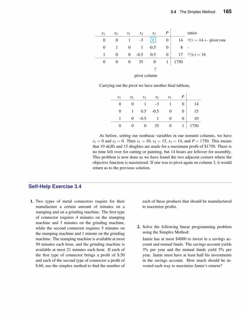
3.4 The Simplex Method 185
x1 x2 s1 s2 s3 P ratios
0 0 1 -3 1 0 14 14/1 = 14← pivot row
0 1 0 1 -0.5 0 8 -
1 0 0 -0.5 0.5 0 17 17/0.5 = 34
0 0 0 35 0 1 1750
↑pivot column
Carrying out the pivot we have another final tableau,
x1 x2 s1 s2 s3 P
0 0 1 -3 1 0 14
0 1 0.5 -0.5 0 0 15
1 0 -0.5 1 0 0 10
0 0 0 35 0 1 1750
As before, setting our nonbasic variables in our nonunit columns, we have
s1 = 0 and s2 = 0. Then x1 = 10, x2 = 15, s3 = 14, and P = 1750. This means
that 10 skiffs and 15 dinghies are made for a maximum profit of $1750. There is
no time left over for cutting or painting, but 14 hours are leftover for assembly.
This problem is now done as we have found the two adjacent corners where the
objective function is maximized. If one was to pivot again on column 3, it would
return us to the previous solution.
Self-Help Exercise 3.4
1. Two types of metal connectors require for their
manufacture a certain amount of minutes on a
stamping and on a grinding machine. The first type
of connector requires 4 minutes on the stamping
machine and 3 minutes on the grinding machine,
while the second connector requires 5 minutes on
the stamping machine and 1 minute on the grinding
machine. The stamping machine is available at most
50 minutes each hour, and the grinding machine is
available at most 21 minutes each hour. If each of
the first type of connector brings a profit of $.50
and each of the second type of connector a profit of
$.60, use the simplex method to find the number of
each of these products that should be manufactured
to maximize profits.
2. Solve the following linear programming problem
using the Simplex Method:
Jamie has at most $4000 to invest in a savings ac-
count and mutual funds. The savings account yields
3% per year and the mutual funds yield 5% per
year. Jamie must have at least half his investments
in the savings account. How much should be in-
vested each way to maximize Jamie’s returns?
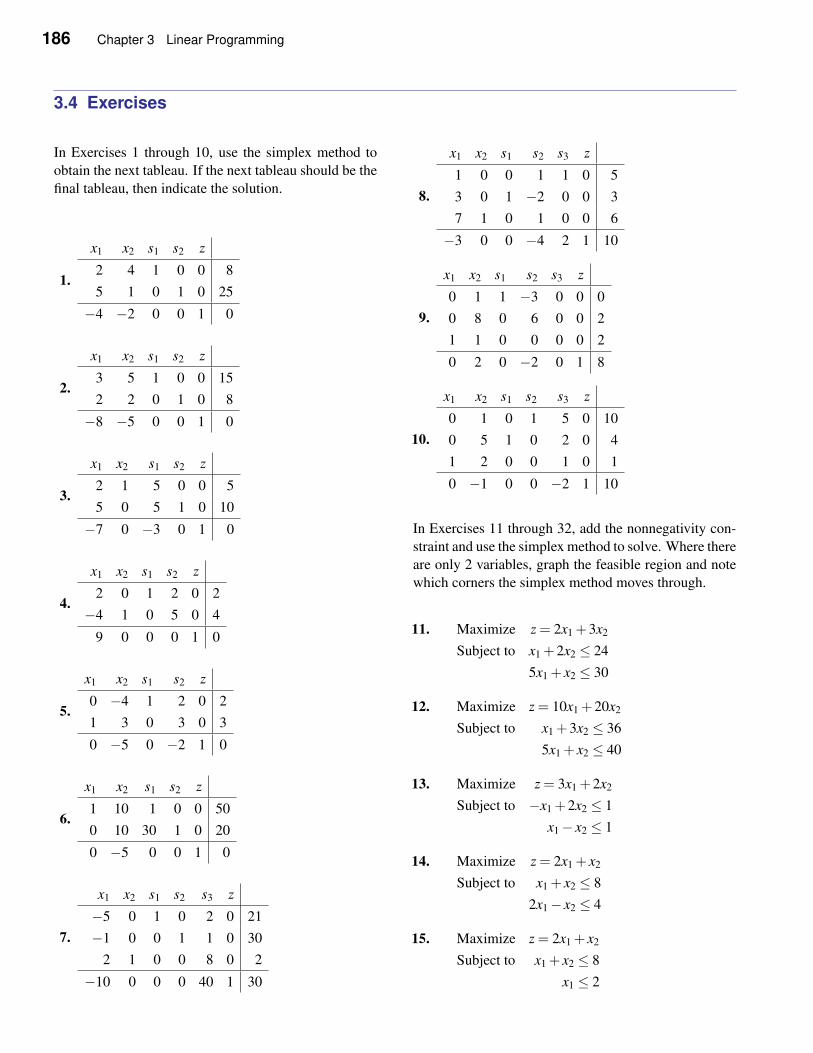
186 Chapter 3 Linear Programming
3.4 Exercises
In Exercises 1 through 10, use the simplex method to
obtain the next tableau. If the next tableau should be the
final tableau, then indicate the solution.
1.
x1 x2 s1 s2 z
2 4 1 0 0 8
5 1 0 1 0 25
−4 −2 0 0 1 0
2.
x1 x2 s1 s2 z
3 5 1 0 0 15
2 2 0 1 0 8
−8 −5 0 0 1 0
3.
x1 x2 s1 s2 z
2 1 5 0 0 5
5 0 5 1 0 10
−7 0 −3 0 1 0
4.
x1 x2 s1 s2 z
2 0 1 2 0 2
−4 1 0 5 0 4
9 0 0 0 1 0
5.
x1 x2 s1 s2 z
0 −4 1 2 0 2
1 3 0 3 0 3
0 −5 0 −2 1 0
6.
x1 x2 s1 s2 z
1 10 1 0 0 50
0 10 30 1 0 20
0 −5 0 0 1 0
7.
x1 x2 s1 s2 s3 z
−5 0 1 0 2 0 21
−1 0 0 1 1 0 30
2 1 0 0 8 0 2
−10 0 0 0 40 1 30
8.
x1 x2 s1 s2 s3 z
1 0 0 1 1 0 5
3 0 1 −2 0 0 3
7 1 0 1 0 0 6
−3 0 0 −4 2 1 10
9.
x1 x2 s1 s2 s3 z
0 1 1 −3 0 0 0
0 8 0 6 0 0 2
1 1 0 0 0 0 2
0 2 0 −2 0 1 8
10.
x1 x2 s1 s2 s3 z
0 1 0 1 5 0 10
0 5 1 0 2 0 4
1 2 0 0 1 0 1
0 −1 0 0 −2 1 10
In Exercises 11 through 32, add the nonnegativity con-
straint and use the simplex method to solve. Where there
are only 2 variables, graph the feasible region and note
which corners the simplex method moves through.
11. Maximize z = 2x1 +3x2
Subject to x1 +2x2 ≤ 24
5x1 + x2 ≤ 30
12. Maximize z = 10x1 +20x2
Subject to x1 +3x2 ≤ 36
5x1 + x2 ≤ 40
13. Maximize z = 3x1 +2x2
Subject to −x1 +2x2 ≤ 1
x1− x2 ≤ 1
14. Maximize z = 2x1 + x2
Subject to x1 + x2 ≤ 8
2x1− x2 ≤ 4
15. Maximize z = 2x1 + x2
Subject to x1 + x2 ≤ 8
x1 ≤ 2
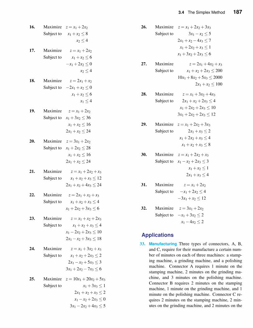
3.4 The Simplex Method 187
16. Maximize z = x1 +2x2
Subject to x1 + x2 ≤ 8
x2 ≤ 4
17. Maximize z = x1 +2x2
Subject to x1 + x2 ≤ 6
−x1 +2x2 ≤ 0
x2 ≤ 4
18. Maximize z = 2x1 + x2
Subject to −2x1 + x2 ≤ 0
x1 + x2 ≤ 6
x1 ≤ 4
19. Maximize z = x1 +2x2
Subject to x1 +3x2 ≤ 36
x1 + x2 ≤ 16
2x1 + x2 ≤ 24
20. Maximize z = 3x1 +2x2
Subject to x1 +2x2 ≤ 28
x1 + x2 ≤ 16
2x1 + x2 ≤ 24
21. Maximize z = x1 +2x2 + x3
Subject to x1 + x2 + x3 ≤ 12
2x1 + x2 +4x3 ≤ 24
22. Maximize z = 2x1 + x2 + x3
Subject to x1 + x2 + x3 ≤ 4
x1 +2x2 +3x3 ≤ 6
23. Maximize z = x1 + x2 +2x3
Subject to x1 + x2 + x3 ≤ 4
x1−2x2 +2x3 ≤ 10
2x1− x2 +3x3 ≤ 18
24. Maximize z = x1 +3x2 + x3
Subject to x1 + x2 +2x3 ≤ 2
2x1− x2 +5x3 ≤ 3
3x1 +2x2−7x3 ≤ 6
25. Maximize z = 10x1 +20x2 +5x3
Subject to x1 +3x3 ≤ 1
2x1 + x2 + x3 ≤ 2
x1− x2 +2x3 ≤ 0
3x1−2x2 +4x3 ≤ 5
26. Maximize z = x1 +2x2 +3x3
Subject to 3x1− x2 ≤ 5
2x1 + x2−4x3 ≤ 7
x1 +2x2 + x3 ≤ 1
x1 +3x2 +2x3 ≤ 6
27. Maximize z = 2x1 +4x2 + x3
Subject to x1 + x2 +2x3 ≤ 200
10x1 +8x2 +5x3 ≤ 2000
2x1 + x2 ≤ 100
28. Maximize z = x1 +3x2 +4x3
Subject to 2x1 + x2 +2x3 ≤ 4
x1 +2x2 +2x3 ≤ 10
3x1 +2x2 +2x3 ≤ 12
29. Maximize z = x1 +2x2 +3x3
Subject to 2x1 + x3 ≤ 2
x1 +2x2 + x3 ≤ 4
x1 + x2 + x3 ≤ 8
30. Maximize z = x1 +2x2 + x3
Subject to x1− x2 +2x3 ≤ 3
x1 + x2 ≤ 1
2x1 + x3 ≤ 4
31. Maximize z = x1 +2x2
Subject to −x1 +2x2 ≤ 4
−3x1 + x2 ≤ 12
32. Maximize z = 3x1 +2x2
Subject to −x1 +3x2 ≤ 2
x1−4x2 ≤ 2
Applications
33. Manufacturing Three types of connectors, A, B,
and C, require for their manufacture a certain num-
ber of minutes on each of three machines: a stamp-
ing machine, a grinding machine, and a polishing
machine. Connector A requires 1 minute on the
stamping machine, 2 minutes on the grinding ma-
chine, and 3 minutes on the polishing machine.
Connector B requires 2 minutes on the stamping
machine, 1 minute on the grinding machine, and 1
minute on the polishing machine. Connector C re-
quires 2 minutes on the stamping machine, 2 min-
utes on the grinding machine, and 2 minutes on the
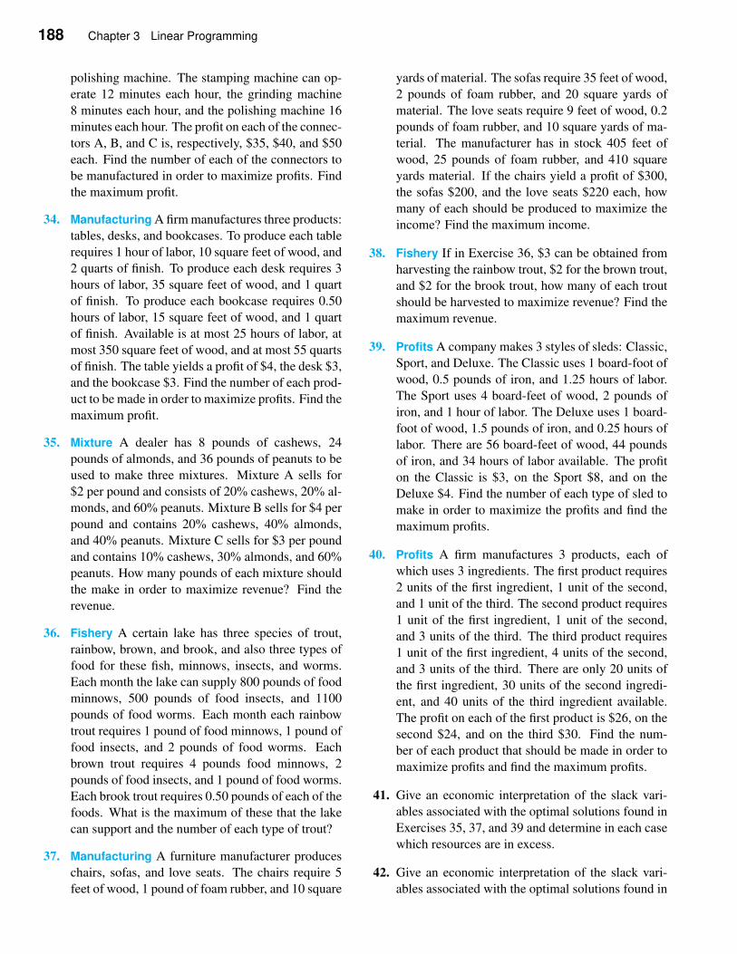
188 Chapter 3 Linear Programming
polishing machine. The stamping machine can op-
erate 12 minutes each hour, the grinding machine
8 minutes each hour, and the polishing machine 16
minutes each hour. The profit on each of the connec-
tors A, B, and C is, respectively, $35, $40, and $50
each. Find the number of each of the connectors to
be manufactured in order to maximize profits. Find
the maximum profit.
34. Manufacturing A firm manufactures three products:
tables, desks, and bookcases. To produce each table
requires 1 hour of labor, 10 square feet of wood, and
2 quarts of finish. To produce each desk requires 3
hours of labor, 35 square feet of wood, and 1 quart
of finish. To produce each bookcase requires 0.50
hours of labor, 15 square feet of wood, and 1 quart
of finish. Available is at most 25 hours of labor, at
most 350 square feet of wood, and at most 55 quarts
of finish. The table yields a profit of $4, the desk $3,
and the bookcase $3. Find the number of each prod-
uct to be made in order to maximize profits. Find the
maximum profit.
35. Mixture A dealer has 8 pounds of cashews, 24
pounds of almonds, and 36 pounds of peanuts to be
used to make three mixtures. Mixture A sells for
$2 per pound and consists of 20% cashews, 20% al-
monds, and 60% peanuts. Mixture B sells for $4 per
pound and contains 20% cashews, 40% almonds,
and 40% peanuts. Mixture C sells for $3 per pound
and contains 10% cashews, 30% almonds, and 60%
peanuts. How many pounds of each mixture should
the make in order to maximize revenue? Find the
revenue.
36. Fishery A certain lake has three species of trout,
rainbow, brown, and brook, and also three types of
food for these fish, minnows, insects, and worms.
Each month the lake can supply 800 pounds of food
minnows, 500 pounds of food insects, and 1100
pounds of food worms. Each month each rainbow
trout requires 1 pound of food minnows, 1 pound of
food insects, and 2 pounds of food worms. Each
brown trout requires 4 pounds food minnows, 2
pounds of food insects, and 1 pound of food worms.
Each brook trout requires 0.50 pounds of each of the
foods. What is the maximum of these that the lake
can support and the number of each type of trout?
37. Manufacturing A furniture manufacturer produces
chairs, sofas, and love seats. The chairs require 5
feet of wood, 1 pound of foam rubber, and 10 square
yards of material. The sofas require 35 feet of wood,
2 pounds of foam rubber, and 20 square yards of
material. The love seats require 9 feet of wood, 0.2
pounds of foam rubber, and 10 square yards of ma-
terial. The manufacturer has in stock 405 feet of
wood, 25 pounds of foam rubber, and 410 square
yards material. If the chairs yield a profit of $300,
the sofas $200, and the love seats $220 each, how
many of each should be produced to maximize the
income? Find the maximum income.
38. Fishery If in Exercise 36, $3 can be obtained from
harvesting the rainbow trout, $2 for the brown trout,
and $2 for the brook trout, how many of each trout
should be harvested to maximize revenue? Find the
maximum revenue.
39. Profits A company makes 3 styles of sleds: Classic,
Sport, and Deluxe. The Classic uses 1 board-foot of
wood, 0.5 pounds of iron, and 1.25 hours of labor.
The Sport uses 4 board-feet of wood, 2 pounds of
iron, and 1 hour of labor. The Deluxe uses 1 board-
foot of wood, 1.5 pounds of iron, and 0.25 hours of
labor. There are 56 board-feet of wood, 44 pounds
of iron, and 34 hours of labor available. The profit
on the Classic is $3, on the Sport $8, and on the
Deluxe $4. Find the number of each type of sled to
make in order to maximize the profits and find the
maximum profits.
40. Profits A firm manufactures 3 products, each of
which uses 3 ingredients. The first product requires
2 units of the first ingredient, 1 unit of the second,
and 1 unit of the third. The second product requires
1 unit of the first ingredient, 1 unit of the second,
and 3 units of the third. The third product requires
1 unit of the first ingredient, 4 units of the second,
and 3 units of the third. There are only 20 units of
the first ingredient, 30 units of the second ingredi-
ent, and 40 units of the third ingredient available.
The profit on each of the first product is $26, on the
second $24, and on the third $30. Find the num-
ber of each product that should be made in order to
maximize profits and find the maximum profits.
41. Give an economic interpretation of the slack vari-
ables associated with the optimal solutions found in
Exercises 35, 37, and 39 and determine in each case
which resources are in excess.
42. Give an economic interpretation of the slack vari-
ables associated with the optimal solutions found in
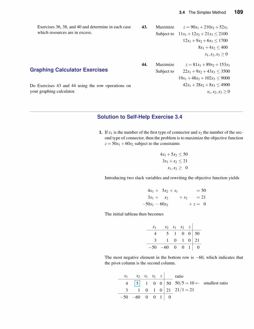
3.4 The Simplex Method 189
Exercises 36, 38, and 40 and determine in each case
which resources are in excess.
Graphing Calculator Exercises
Do Exercises 43 and 44 using the row operations on
your graphing calculator.
43. Maximize z = 90x1 +210x2 +52x3
Subject to 11x1 +12x2 +21x3 ≤ 2100
12x1 +9x2 +6x3 ≤ 1700
8x1 +4x2 ≤ 400
x1,x2,x3 ≥ 0
44. Maximize z = 81x1 +89x2 +153x3
Subject to 22x1 +9x2 +43x3 ≤ 3500
19x1 +48x2 +102x3 ≤ 9000
42x1 +28x2 +8x3 ≤ 4900
x1,x2,x3 ≥ 0
Solution to Self-Help Exercise 3.4
1. If x1 is the number of the first type of connector and x2 the number of the sec-
ond type of connector, then the problem is to maximize the objective function
z = 50x1 +60x2 subject to the constraints
4x1 +5x2 ≤ 50
3x1 + x2 ≤ 21
x1,x2 ≥ 0
Introducing two slack variables and rewriting the objective function yields
4x1 + 5x2 + s1 = 50
3x1 + x2 + s2 = 21
−50x1 − 60x2 + z = 0
The initial tableau then becomes
x1 x2 s1 s2 z
4 5 1 0 0 50
3 1 0 1 0 21
−50 −60 0 0 1 0
The most negative element in the bottom row is −60, which indicates that
the pivot column is the second column.
x1 x2 s1 s2 z
4 5 1 0 0 50
3 1 0 1 0 21
−50 −60 0 0 1 0
ratio
50/5 = 10← smallest ratio
21/1 = 21
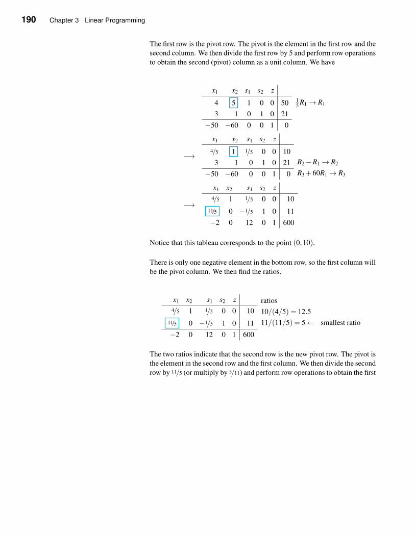
190 Chapter 3 Linear Programming
The first row is the pivot row. The pivot is the element in the first row and the
second column. We then divide the first row by 5 and perform row operations
to obtain the second (pivot) column as a unit column. We have
x1 x2 s1 s2 z
4 5 1 0 0 50
3 1 0 1 0 21
−50 −60 0 0 1 0
15 R1→ R1
−→
x1 x2 s1 s2 z
4/5 1 1/5 0 0 10
3 1 0 1 0 21
−50 −60 0 0 1 0
R2−R1→ R2
R3 +60R1→ R3
−→
x1 x2 s1 s2 z
4/5 1 1/5 0 0 10
11/5 0 −1/5 1 0 11
−2 0 12 0 1 600
Notice that this tableau corresponds to the point (0,10).
There is only one negative element in the bottom row, so the first column will
be the pivot column. We then find the ratios.
x1 x2 s1 s2 z
4/5 1 1/5 0 0 10
11/5 0 −1/5 1 0 11
−2 0 12 0 1 600
ratios
10/(4/5) = 12.5
11/(11/5) = 5← smallest ratio
The two ratios indicate that the second row is the new pivot row. The pivot is
the element in the second row and the first column. We then divide the second
row by 11/5 (or multiply by 5/11) and perform row operations to obtain the first
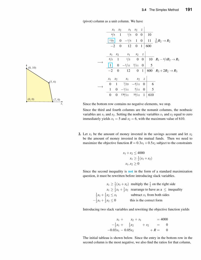
3.4 The Simplex Method 191
(pivot) column as a unit column. We have
x1 x2 s1 s2 z
4/5 1 1/5 0 0 10
11/5 0 −1/5 1 0 11 511 R2→ R2
−2 0 12 0 1 600
−→
x1 x2 s1 s2 z
4/5 1 1/5 0 0 10 R1− 4/5R2→ R1
1 0 −1/11 5/11 0 5
−2 0 12 0 1 600 R3 +2R2→ R3
−→
x1 x2 s1 s2 z
0 1 7/55 −4/11 0 6
1 0 −1/11 5/11 0 5
0 0 130/11 10/11 1 610
Since the bottom row contains no negative elements, we stop.
Since the third and fourth columns are the nonunit columns, the nonbasic
variables are s1 and s2. Setting the nonbasic variables s1 and s2 equal to zero
immediately yields x1 = 5 and x2 = 6, with the maximum value of 610.
2. Let x1 be the amount of money invested in the savings account and let x2
be the amount of money invested in the mutual funds. Then we need to
maximize the objective function R = 0.3x1 +0.5x2 subject to the constraints
x1 + x2 ≤ 4000
x1 ≥ 12(x1 + x2)
x1,x2 ≥ 0
Since the second inequality is not in the form of a standard maximization
question, it must be rewritten before introducing slack variables.
x1 ≥ 12(x1 + x2) multiply the 1
2on the right side
x1 ≥ 12 x1 +
12 x2 rearrange to have as a ≤ inequality
12 x1 +
12 x2 ≤ x1 subtract x1 from both sides
− 12x1 +
12x2 ≤ 0 this is the correct form
Introducing two slack variables and rewriting the objective function yields
x1 + x2 + s1 = 4000
− 12 x1 + 1
2 x2 + s2 = 0
−0.03x1 − 0.05x2 + R = 0
The initial tableau is shown below. Since the entry in the bottom row in the
second column is the most negative, we also find the ratios for that column,
192 Chapter 3 Linear Programming
x1 x2 s1 s2 R
1 1 1 0 0 4000
− 12 0.5 0 1 0 0
−0.03 −0.05 0 0 1 0
ratios
4000/1 = 4000
0/(1/2) = 0← smallest ratio
Note that 0 is the smallest possible non-negative number so if the ratio is 0, it
will always be the pivot row. Performing the pivot we have the tableau shown
below with the most negative entry in the bottom row in the first column.
x1 x2 s1 s2 R
2 0 1 −2 0 4000
−1 1 0 2 0 0
−0.08 0 0 0.1 1 0
ratios
4000/2 = 2000← smallest ratio
do not pivot on negative numbers
After performing the pivot on row 1, column 1 we have our final tableau,
x1 x2 s1 s2 R
1 0 0.5 −1 0 2000
0 1 0.5 1 0 2000
0 0 0.4 0.2 1 160
Reading the solution from the final tableau, x1 = 2000, x2 = 2000. Jamie will
invest $2000 in savings and $2000 in mutual funds to have a total return of
$160.
3.5 Post-Optimal Analysis
In this chapter we learned how to find an optimal solution to a linear program-
ming problem in two dimensions or more dimensions. After an optimal solution
to an application problem has been found, further analysis is usually required.
For example, are any resources left over? If this is the case, then management
should consider reallocating or reducing this resource. What if the profit per item
was different? Will the optimal solution stay the same? And finally, what if more
of a resource could be obtained? Which resource should we increase to have a
higher profit? All these concepts will be explored in the context of the following
detailed examples.
✧ Determining Excess Resources
EXAMPLE 1 Building Skiffs and Dinghies Consider the wooden-boat man-
ufacturing problem solved in previous sections. Recall that 10 dinghies and 15
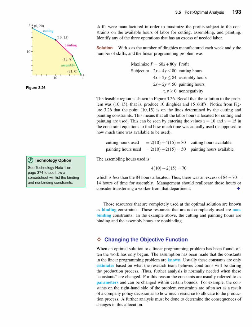
3.5 Post-Optimal Analysis 193
skiffs were manufactured in order to maximize the profits subject to the con-
straints on the available hours of labor for cutting, assembling, and painting.
Identify any of the three operations that has an excess of needed labor.
Solution With x as the number of dinghies manufactured each week and y the
number of skiffs, and the linear programming problem was
Figure 3.26
Maximize P = 60x+80y Profit
Subject to 2x+4y≤ 80 cutting hours
4x+2y≤ 84 assembly hours
2x+2y≤ 50 painting hours
x,y≥ 0 nonnegativity
The feasible region is shown in Figure 3.26. Recall that the solution to the prob-
lem was (10,15), that is, produce 10 dinghies and 15 skiffs. Notice from Fig-
ure 3.26 that the point (10,15) is on the lines determined by the cutting and
painting constraints. This means that all the labor hours allocated for cutting and
painting are used. This can be seen by entering the values x = 10 and y = 15 in
the constraint equations to find how much time was actually used (as opposed to
how much time was available to be used).
cutting hours used = 2(10)+4(15) = 80 cutting hours available
painting hours used = 2(10)+2(15) = 50 painting hours available
The assembling hours used is
4(10)+2(15) = 70
which is less than the 84 hours allocated. Thus, there was an excess of 84−70 =14 hours of time for assembly. Management should reallocate those hours or
consider transferring a worker from that department. ✦
TTT©©© Technology Option
See Technology Note 1 on
page 374 to see how a
spreadsheet will list the binding
and nonbinding constraints.
Those resources that are completely used at the optimal solution are known
as binding constraints. Those resources that are not completely used are non-
binding constraints. In the example above, the cutting and painting hours are
binding and the assembly hours are nonbinding.
✧ Changing the Objective Function
When an optimal solution to a linear programming problem has been found, of-
ten the work has only begun. The assumption has been made that the constants
in the linear programming problem are known. Usually these constants are only
estimates based on what the research team believes conditions will be during
the production process. Thus, further analysis is normally needed when these
“constants” are changed. For this reason the constants are usually referred to as
parameters and can be changed within certain bounds. For example, the con-
stants on the right-hand side of the problem constraints are often set as a result
of a company policy decision as to how much resource to allocate to the produc-
tion process. A further analysis must be done to determine the consequences of
changes in this allocation.
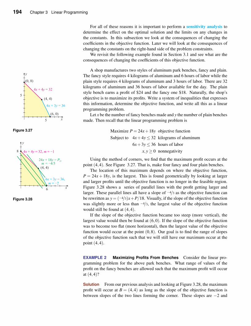
194 Chapter 3 Linear Programming
For all of these reasons it is important to perform a sensitivity analysis to
determine the effect on the optimal solution and the limits on any changes in
the constants. In this subsection we look at the consequences of changing the
coefficients in the objective function. Later we will look at the consequences of
changing the constants on the right-hand side of the problem constraints.
We revisit the following example found in Section 3.1 and see what are the
consequences of changing the coefficients of this objective function.
A shop manufactures two styles of aluminum park benches, fancy and plain.
The fancy style requires 4 kilograms of aluminum and 6 hours of labor while the
plain style requires 4 kilograms of aluminum and 3 hours of labor. There are 32
kilograms of aluminum and 36 hours of labor available for the day. The plain
style bench earns a profit of $24 and the fancy one $18. Naturally, the shop’s
objective is to maximize its profits. Write a system of inequalities that expresses
this information, determine the objective function, and write all this as a linear
programming problem.
Let x be the number of fancy benches made and y the number of plain benches
made. Then recall that the linear programming problem is
Figure 3.27 Maximize P = 24x+18y objective function
Subject to 4x+4y≤ 32 kilograms of aluminum
6x+3y≤ 36 hours of labor
x,y≥ 0 nonnegativity
Using the method of corners, we find that the maximum profit occurs at the
point (4,4). See Figure 3.27. That is, make four fancy and four plain benches.
The location of this maximum depends on where the objective function,
P = 24x+ 18y, is the largest. This is found geometrically by looking at larger
and larger profits until the objective function is no longer in the feasible region.
Figure 3.28 shows a series of parallel lines with the profit getting larger and
Figure 3.28
larger. These parallel lines all have a slope of −4/3 as the objective function can
be rewritten as y = (−4/3)x+P/18. Visually, if the slope of the objective function
was slightly more or less than −4/3, the largest value of the objective function
would still be found at (4,4).If the slope of the objective function became too steep (more vertical), the
largest value would then be found at (6,0). If the slope of the objective function
was to become too flat (more horizontal), then the largest value of the objective
function would occur at the point (0,8). Our goal is to find the range of slopes
of the objective function such that we will still have our maximum occur at the
point (4,4).
EXAMPLE 2 Maximizing Profits From Benches Consider the linear pro-
gramming problem for the above park benches. What range of values of the
profit on the fancy benches are allowed such that the maximum profit will occur
at (4,4)?
Solution From our previous analysis and looking at Figure 3.28, the maximum
profit will occur at B = (4,4) as long as the slope of the objective function is
between slopes of the two lines forming the corner. These slopes are −2 and
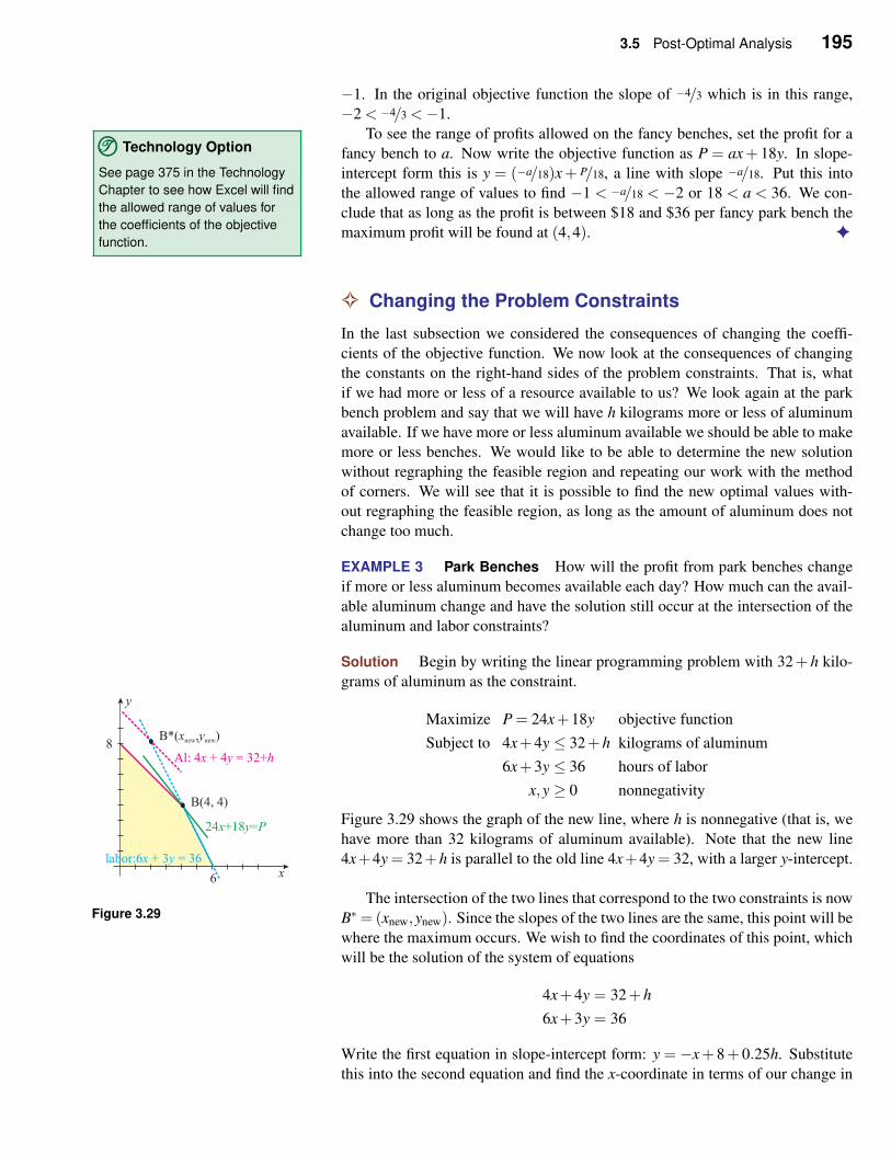
3.5 Post-Optimal Analysis 195
−1. In the original objective function the slope of −4/3 which is in this range,
−2 < −4/3 <−1.
To see the range of profits allowed on the fancy benches, set the profit for a
fancy bench to a. Now write the objective function as P = ax+ 18y. In slope-
intercept form this is y = (−a/18)x+ P/18, a line with slope −a/18. Put this into
the allowed range of values to find −1 < −a/18 < −2 or 18 < a < 36. We con-
TTT©©© Technology Option
See page 375 in the Technology
Chapter to see how Excel will find
the allowed range of values for
the coefficients of the objective
function.
clude that as long as the profit is between $18 and $36 per fancy park bench the
maximum profit will be found at (4,4). ✦
✧ Changing the Problem Constraints
In the last subsection we considered the consequences of changing the coeffi-
cients of the objective function. We now look at the consequences of changing
the constants on the right-hand sides of the problem constraints. That is, what
if we had more or less of a resource available to us? We look again at the park
bench problem and say that we will have h kilograms more or less of aluminum
available. If we have more or less aluminum available we should be able to make
more or less benches. We would like to be able to determine the new solution
without regraphing the feasible region and repeating our work with the method
of corners. We will see that it is possible to find the new optimal values with-
out regraphing the feasible region, as long as the amount of aluminum does not
change too much.
EXAMPLE 3 Park Benches How will the profit from park benches change
if more or less aluminum becomes available each day? How much can the avail-
able aluminum change and have the solution still occur at the intersection of the
aluminum and labor constraints?
Solution Begin by writing the linear programming problem with 32+ h kilo-
grams of aluminum as the constraint.
Maximize P = 24x+18y objective function
Subject to 4x+4y ≤ 32+h kilograms of aluminum
6x+3y ≤ 36 hours of labor
x,y ≥ 0 nonnegativity
Figure 3.29 shows the graph of the new line, where h is nonnegative (that is, we
have more than 32 kilograms of aluminum available). Note that the new line
4x+4y = 32+h is parallel to the old line 4x+4y = 32, with a larger y-intercept.
Figure 3.29The intersection of the two lines that correspond to the two constraints is now
B∗ = (xnew,ynew). Since the slopes of the two lines are the same, this point will be
where the maximum occurs. We wish to find the coordinates of this point, which
will be the solution of the system of equations
4x+4y = 32+h
6x+3y = 36
Write the first equation in slope-intercept form: y = −x+ 8+ 0.25h. Substitute
this into the second equation and find the x-coordinate in terms of our change in
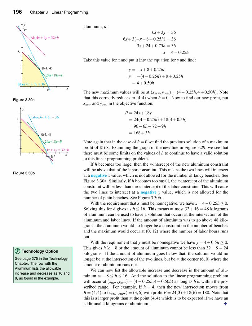
196 Chapter 3 Linear Programming
aluminum, h:
6x+3y = 36
6x+3(−x+8+0.25h) = 36
3x+24+0.75h = 36
x = 4−0.25h
Take this value for x and put it into the equation for y and find:
Figure 3.30a
y = −x+8+0.25h
y = −(4−0.25h)+8+0.25h
= 4+0.50h
The new maximum values will be at (xnew,ynew) = (4−0.25h,4+0.50h). Note
that this correctly reduces to (4,4) when h = 0. Now to find our new profit, put
xnew and ynew in the objective function:
P = 24x+18y
= 24(4−0.25h)+18(4+0.5h)
= 96−6h+72+9h
= 168+3h
Note again that in the case of h = 0 we find the previous solution of a maximum
profit of $168. Examining the graph of the new line in Figure 3.29, we see that
there must be some limits on the values of h to continue to have a valid solution
to this linear programming problem.
Figure 3.30b
If h becomes too large, then the y-intercept of the new aluminum constraint
will be above that of the labor constraint. This means the two lines will intersect
at a negative x value, which is not allowed for the number of fancy benches. See
Figure 3.30a. Similarly, if h becomes too small, the x-intercept of the aluminum
constraint will be less than the x-intercept of the labor constraint. This will cause
the two lines to intersect at a negative y value, which is not allowed for the
number of plain benches. See Figure 3.30b.
With the requirement that x must be nonnegative, we have x = 4−0.25h≥ 0.
Solving this for h gives us h ≤ 16. This means at most 32+ 16 = 48 kilograms
of aluminum can be used to have a solution that occurs at the intersection of the
aluminum and labor lines. If the amount of aluminum was to go above 48 kilo-
grams, the aluminum would no longer be a constraint on the number of benches
and the maximum would occur at (0, 12) where the number of labor hours runs
out.
With the requirement that y must be nonnegative we have y = 4+ 0.5h ≥ 0.
This gives h ≥ −8 or the amount of aluminum cannot be less than 32− 8 = 24
kilograms. If the amount of aluminum goes below that, the solution would no
longer be at the intersection of the two lines, but be at the corner (6, 0) where the
amount of aluminum runs out.
TTT©©© Technology Option
See page 375 in the Technology
Chapter. The row with the
Aluminum lists the allowable
increase and decrease as 16 and
8, as found in the example.
We can now list the allowable increase and decrease in the amount of alu-
minum as −8 ≤ h ≤ 16. And the solution to the linear programming problem
will occur at (xnew,ynew) = (4−0.25h,4+0.50h) as long as h is within the pro-
scribed range. For example, if h = 4, then the new intersection moves from
B = (4,4) to (xnew,ynew) = (3,6) with profit P = 24(3)+18(6) = 180. Note that
this is a larger profit than at the point (4,4) which is to be expected if we have an
additional 4 kilograms of aluminum. ✦
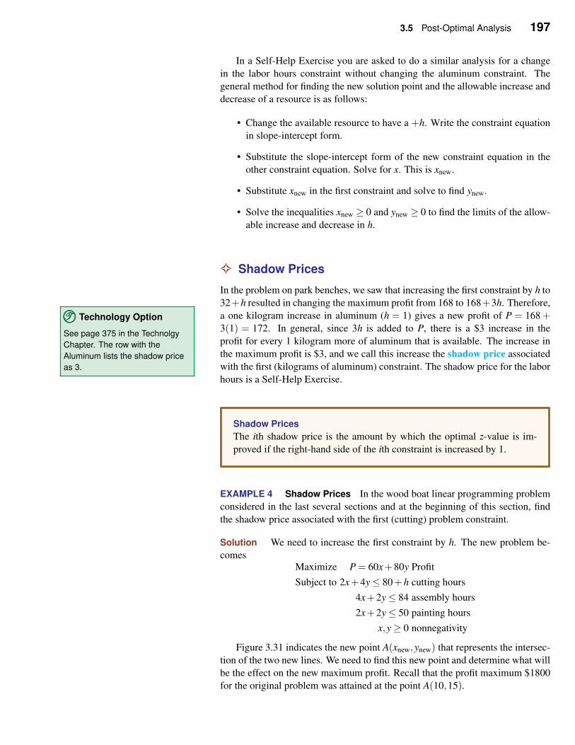
3.5 Post-Optimal Analysis 197
In a Self-Help Exercise you are asked to do a similar analysis for a change
in the labor hours constraint without changing the aluminum constraint. The
general method for finding the new solution point and the allowable increase and
decrease of a resource is as follows:
• Change the available resource to have a +h. Write the constraint equation
in slope-intercept form.
• Substitute the slope-intercept form of the new constraint equation in the
other constraint equation. Solve for x. This is xnew.
• Substitute xnew in the first constraint and solve to find ynew.
• Solve the inequalities xnew ≥ 0 and ynew ≥ 0 to find the limits of the allow-
able increase and decrease in h.
✧ Shadow Prices
In the problem on park benches, we saw that increasing the first constraint by h to
32+h resulted in changing the maximum profit from 168 to 168+3h. Therefore,
a one kilogram increase in aluminum (h = 1) gives a new profit of P = 168+3(1) = 172. In general, since 3h is added to P, there is a $3 increase in the
profit for every 1 kilogram more of aluminum that is available. The increase in
TTT©©© Technology Option
See page 375 in the Technolgy
Chapter. The row with the
Aluminum lists the shadow price
as 3.
the maximum profit is $3, and we call this increase the shadow price associated
with the first (kilograms of aluminum) constraint. The shadow price for the labor
hours is a Self-Help Exercise.
Shadow Prices
The ith shadow price is the amount by which the optimal z-value is im-
proved if the right-hand side of the ith constraint is increased by 1.
EXAMPLE 4 Shadow Prices In the wood boat linear programming problem
considered in the last several sections and at the beginning of this section, find
the shadow price associated with the first (cutting) problem constraint.
Solution We need to increase the first constraint by h. The new problem be-
comesMaximize P = 60x+80y Profit
Subject to 2x+4y≤ 80+h cutting hours
4x+2y≤ 84 assembly hours
2x+2y≤ 50 painting hours
x,y≥ 0 nonnegativity
Figure 3.31 indicates the new point A(xnew,ynew) that represents the intersec-
tion of the two new lines. We need to find this new point and determine what will
be the effect on the new maximum profit. Recall that the profit maximum $1800
for the original problem was attained at the point A(10,15).
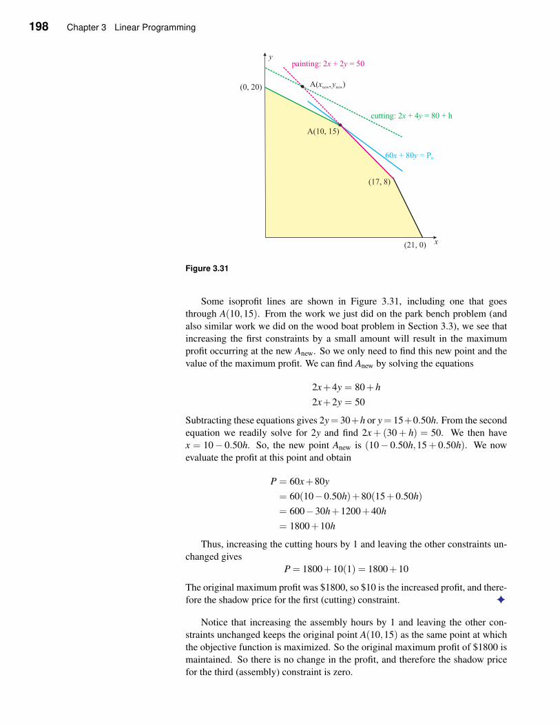
198 Chapter 3 Linear Programming
Figure 3.31
Some isoprofit lines are shown in Figure 3.31, including one that goes
through A(10,15). From the work we just did on the park bench problem (and
also similar work we did on the wood boat problem in Section 3.3), we see that
increasing the first constraints by a small amount will result in the maximum
profit occurring at the new Anew. So we only need to find this new point and the
value of the maximum profit. We can find Anew by solving the equations
2x+4y = 80+h
2x+2y = 50
Subtracting these equations gives 2y= 30+h or y= 15+0.50h. From the second
equation we readily solve for 2y and find 2x + (30 + h) = 50. We then have
x = 10− 0.50h. So, the new point Anew is (10− 0.50h,15+ 0.50h). We now
evaluate the profit at this point and obtain
P = 60x+80y
= 60(10−0.50h)+80(15+0.50h)
= 600−30h+1200+40h
= 1800+10h
Thus, increasing the cutting hours by 1 and leaving the other constraints un-
changed gives
P = 1800+10(1) = 1800+10
The original maximum profit was $1800, so $10 is the increased profit, and there-
fore the shadow price for the first (cutting) constraint. ✦
Notice that increasing the assembly hours by 1 and leaving the other con-
straints unchanged keeps the original point A(10,15) as the same point at which
the objective function is maximized. So the original maximum profit of $1800 is
maintained. So there is no change in the profit, and therefore the shadow price
for the third (assembly) constraint is zero.
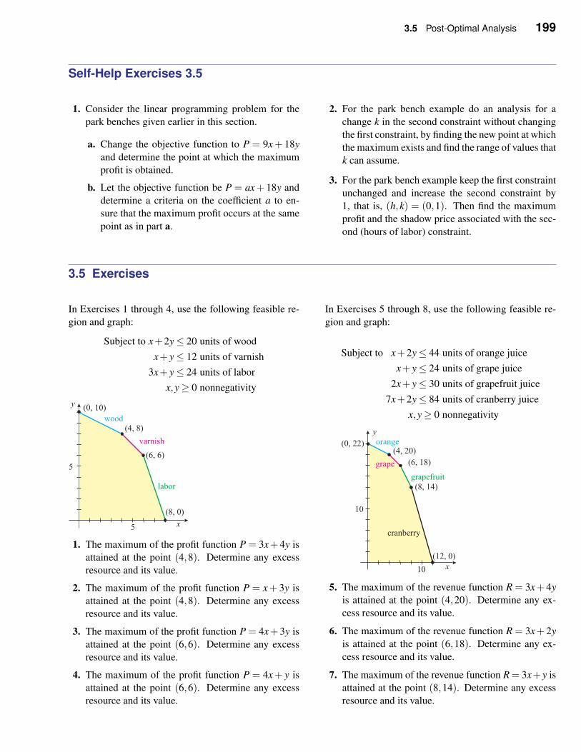
3.5 Post-Optimal Analysis 199
Self-Help Exercises 3.5
1. Consider the linear programming problem for the
park benches given earlier in this section.
a. Change the objective function to P = 9x+ 18y
and determine the point at which the maximum
profit is obtained.
b. Let the objective function be P = ax+ 18y and
determine a criteria on the coefficient a to en-
sure that the maximum profit occurs at the same
point as in part a.
2. For the park bench example do an analysis for a
change k in the second constraint without changing
the first constraint, by finding the new point at which
the maximum exists and find the range of values that
k can assume.
3. For the park bench example keep the first constraint
unchanged and increase the second constraint by
1, that is, (h,k) = (0,1). Then find the maximum
profit and the shadow price associated with the sec-
ond (hours of labor) constraint.
3.5 Exercises
In Exercises 1 through 4, use the following feasible re-
gion and graph:
Subject to x+2y≤ 20 units of wood
x+ y≤ 12 units of varnish
3x+ y≤ 24 units of labor
x,y≥ 0 nonnegativity
1. The maximum of the profit function P = 3x+ 4y is
attained at the point (4,8). Determine any excess
resource and its value.
2. The maximum of the profit function P = x+ 3y is
attained at the point (4,8). Determine any excess
resource and its value.
3. The maximum of the profit function P = 4x+ 3y is
attained at the point (6,6). Determine any excess
resource and its value.
4. The maximum of the profit function P = 4x+ y is
attained at the point (6,6). Determine any excess
resource and its value.
In Exercises 5 through 8, use the following feasible re-
gion and graph:
Subject to x+2y≤ 44 units of orange juice
x+ y≤ 24 units of grape juice
2x+ y≤ 30 units of grapefruit juice
7x+2y≤ 84 units of cranberry juice
x,y≥ 0 nonnegativity
5. The maximum of the revenue function R = 3x+ 4y
is attained at the point (4,20). Determine any ex-
cess resource and its value.
6. The maximum of the revenue function R = 3x+ 2y
is attained at the point (6,18). Determine any ex-
cess resource and its value.
7. The maximum of the revenue function R = 3x+y is
attained at the point (8,14). Determine any excess
resource and its value.
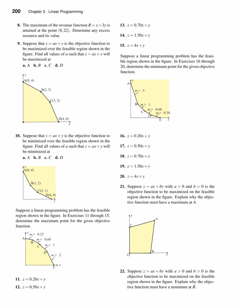
200 Chapter 3 Linear Programming
8. The maximum of the revenue function R = x+3y is
attained at the point (0,22). Determine any excess
resource and its value.
9. Suppose that z = ax+ y is the objective function to
be maximized over the feasible region shown in the
figure. Find all values of a such that z = ax+ y will
be maximized at
a. A b. B c. C d. D
10. Suppose that z = ax+ y is the objective function to
be minimized over the feasible region shown in the
figure. Find all values of a such that z = ax+ y will
be minimized at
a. A b. B c. C d. D
Suppose a linear programming problem has the feasible
region shown in the figure. In Exercises 11 through 15,
determine the maximum point for the given objective
function.
11. z = 0.20x+ y
12. z = 0.50x+ y
13. z = 0.70x+ y
14. z = 1.50x+ y
15. z = 4x+ y
Suppose a linear programming problem has the feasi-
ble region shown in the figure. In Exercises 16 through
20, determine the minimum point for the given objective
function.
16. z = 0.20x+ y
17. z = 0.50x+ y
18. z = 0.70x+ y
19. z = 1.50x+ y
20. z = 4x+ y
21. Suppose z = ax + by with a > 0 and b > 0 is the
objective function to be maximized on the feasible
region shown in the figure. Explain why the objec-
tive function must have a maximum at A.
22. Suppose z = ax + by with a > 0 and b > 0 is the
objective function to be maximized on the feasible
region shown in the figure. Explain why the objec-
tive function must have a minimum at B.
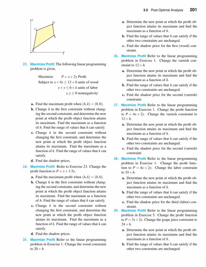
3.5 Post-Optimal Analysis 201
23. Maximize Profit The following linear programming
problem is given.
Maximize P = x+2y Profit
Subject to x+4y≤ 12+h units of wood
x+ y≤ 6+ k units of labor
x,y≥ 0 nonnegativity
a. Find the maximum profit when (h,k) = (0,0).
b. Change h in the first constraint without chang-
ing the second constraint, and determine the new
point at which the profit object function attains
its maximum. Find the maximum as a function
of h. Find the range of values that h can satisfy.
c. Change k in the second constraint without
changing the first constraint, and determine the
new point at which the profit object function
attains its maximum. Find the maximum as a
function of k. Find the range of values that k can
satisfy.
d. Find the shadow prices.
24. Maximize Profit Refer to Exercise 23. Change the
profit function to P = x+1.5y.
a. Find the maximum profit when (h,k) = (0,0).
b. Change h in the first constraint without chang-
ing the second constraint, and determine the new
point at which the profit object function attains
its maximum. Find the maximum as a function
of h. Find the range of values that h can satisfy.
c. Change k in the second constraint without
changing the first constraint, and determine the
new point at which the profit object function
attains its maximum. Find the maximum as a
function of k. Find the range of values that k can
satisfy.
d. Find the shadow prices.
25. Maximize Profit Refer to the linear programming
problem in Exercise 1. Change the wood constraint
to 20+h.
a. Determine the new point at which the profit ob-
ject function attains its maximum and find the
maximum as a function of h.
b. Find the range of values that h can satisfy if the
other two constraints are unchanged.
c. Find the shadow price for the first (wood) con-
straint.
26. Maximize Profit Refer to the linear programming
problem in Exercise 1. Change the varnish con-
straint to 12+h.
a. Determine the new point at which the profit ob-
ject function attains its maximum and find the
maximum as a function of h.
b. Find the range of values that h can satisfy if the
other two constraints are unchanged.
c. Find the shadow price for the second (varnish)
constraint.
27. Maximize Profit Refer to the linear programming
problem in Exercise 1. Change the profit function
to P = 4x + 2y. Change the varnish constraint to
12+h.
a. Determine the new point at which the profit ob-
ject function attains its maximum and find the
maximum as a function of h.
b. Find the range of values that h can satisfy if the
other two constraints are unchanged.
c. Find the shadow price for the second (varnish)
constraint.
28. Maximize Profit Refer to the linear programming
problem in Exercise 1. Change the profit func-
tion to P = 4x + 2y. Change the labor constraint
to 24+h.
a. Determine the new point at which the profit ob-
ject function attains its maximum and find the
maximum as a function of h.
b. Find the range of values that h can satisfy if the
other two constraints are unchanged.
c. Find the shadow price for the third (labor) con-
straint.29. Maximize Profit Refer to the linear programming
problem in Exercise 5. Change the profit function
to P = 3x+2y. Change the grape juice constraint to
24+h.
a. Determine the new point at which the profit ob-
ject function attains its maximum and find the
maximum as a function of h.
b. Find the range of values that h can satisfy if the
other two constraints are unchanged.
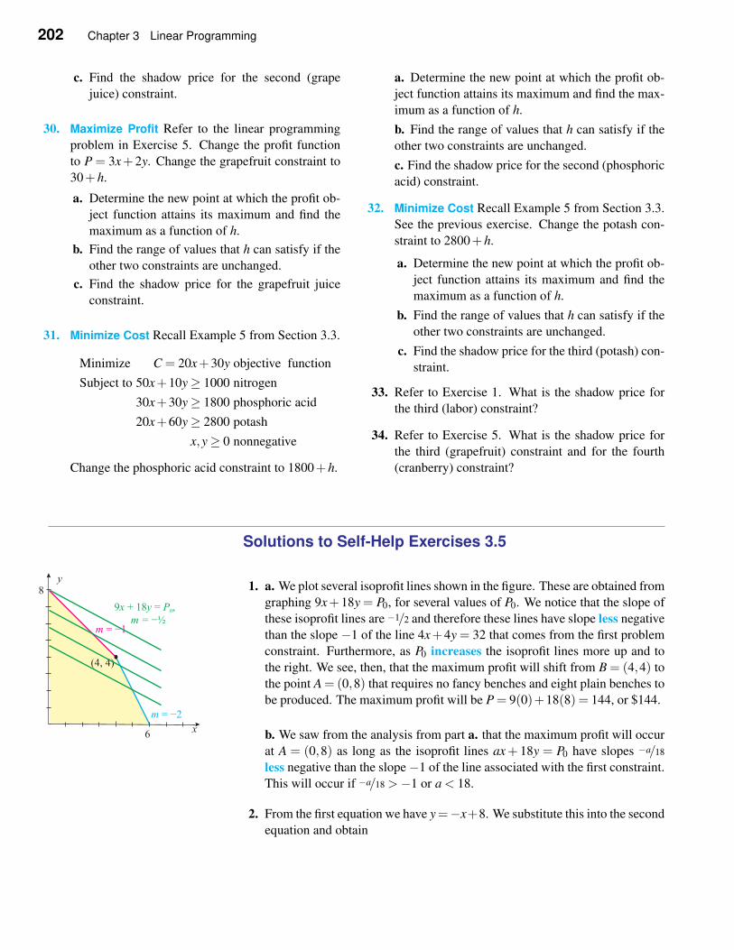
202 Chapter 3 Linear Programming
c. Find the shadow price for the second (grape
juice) constraint.
30. Maximize Profit Refer to the linear programming
problem in Exercise 5. Change the profit function
to P = 3x+ 2y. Change the grapefruit constraint to
30+h.
a. Determine the new point at which the profit ob-
ject function attains its maximum and find the
maximum as a function of h.
b. Find the range of values that h can satisfy if the
other two constraints are unchanged.
c. Find the shadow price for the grapefruit juice
constraint.
31. Minimize Cost Recall Example 5 from Section 3.3.
Minimize C = 20x+30y objective function
Subject to 50x+10y≥ 1000 nitrogen
30x+30y≥ 1800 phosphoric acid
20x+60y≥ 2800 potash
x,y≥ 0 nonnegative
Change the phosphoric acid constraint to 1800+h.
a. Determine the new point at which the profit ob-
ject function attains its maximum and find the max-
imum as a function of h.
b. Find the range of values that h can satisfy if the
other two constraints are unchanged.
c. Find the shadow price for the second (phosphoric
acid) constraint.
32. Minimize Cost Recall Example 5 from Section 3.3.
See the previous exercise. Change the potash con-
straint to 2800+h.
a. Determine the new point at which the profit ob-
ject function attains its maximum and find the
maximum as a function of h.
b. Find the range of values that h can satisfy if the
other two constraints are unchanged.
c. Find the shadow price for the third (potash) con-
straint.
33. Refer to Exercise 1. What is the shadow price for
the third (labor) constraint?
34. Refer to Exercise 5. What is the shadow price for
the third (grapefruit) constraint and for the fourth
(cranberry) constraint?
Solutions to Self-Help Exercises 3.5
1. a. We plot several isoprofit lines shown in the figure. These are obtained from
graphing 9x+18y = P0, for several values of P0. We notice that the slope of
these isoprofit lines are −1/2 and therefore these lines have slope less negative
than the slope −1 of the line 4x+4y = 32 that comes from the first problem
constraint. Furthermore, as P0 increases the isoprofit lines more up and to
the right. We see, then, that the maximum profit will shift from B = (4,4) to
the point A = (0,8) that requires no fancy benches and eight plain benches to
be produced. The maximum profit will be P = 9(0)+18(8) = 144, or $144.
b. We saw from the analysis from part a. that the maximum profit will occur
at A = (0,8) as long as the isoprofit lines ax+ 18y = P0 have slopes −a/18
less negative than the slope−1 of the line associated with the first constraint.
This will occur if −a/18 >−1 or a < 18.
2. From the first equation we have y=−x+8. We substitute this into the second
equation and obtain
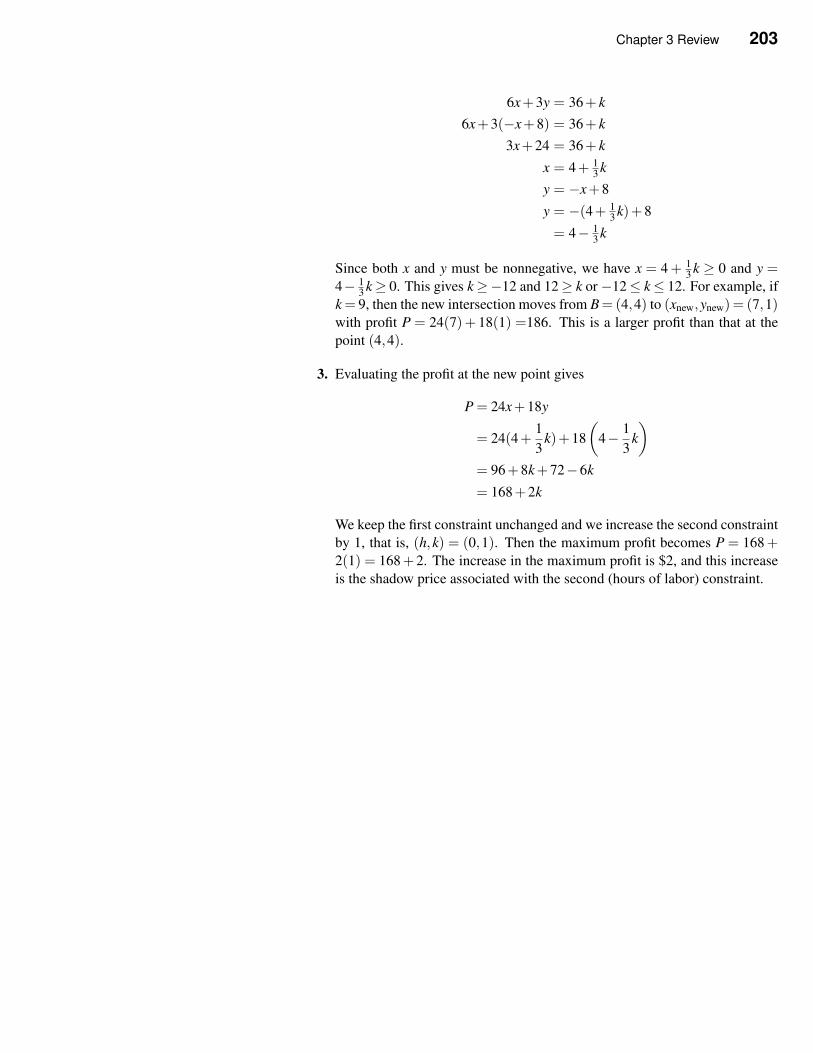
Chapter 3 Review 203
6x+3y = 36+ k
6x+3(−x+8) = 36+ k
3x+24 = 36+ k
x = 4+ 13 k
y = −x+8
y = −(4+ 13k)+8
= 4− 13 k
Since both x and y must be nonnegative, we have x = 4+ 13 k ≥ 0 and y =
4− 13 k≥ 0. This gives k≥−12 and 12≥ k or−12≤ k≤ 12. For example, if
k = 9, then the new intersection moves from B= (4,4) to (xnew,ynew) = (7,1)with profit P = 24(7)+ 18(1) =186. This is a larger profit than that at the
point (4,4).
3. Evaluating the profit at the new point gives
P = 24x+18y
= 24(4+1
3k)+18
(
4− 1
3k
)
= 96+8k+72−6k
= 168+2k
We keep the first constraint unchanged and we increase the second constraint
by 1, that is, (h,k) = (0,1). Then the maximum profit becomes P = 168+2(1) = 168+2. The increase in the maximum profit is $2, and this increase
is the shadow price associated with the second (hours of labor) constraint.
204 Chapter 3 Linear Programming
Review
✧ Summary Outline
• A linear inequality is an inequality of the form
ax+by < c or ≤ c or > c or ≥ c
• The feasible region of a system of inequalities is the set of points that
satisfies all the inequalities in the system.
• Graphing a Linear Inequality
The following steps show how to graph the linear inequality
ax+by < c or ≤ c or > c or ≥ c
1. First graph the straight line L given by ax+ by = c, using a dotted
line if the inequalities “<” or “>” are given and a solid line if the in-
equalities “≤” or “≥” are given. The dotted line indicates the straight
line L is not part of the solution graph, while the solid line indicates
that the line L is part of the solution graph.
2. Pick any convenient test point not on line L and evaluate the inequal-
ity at that test point. If the inequality is true, then the solution graph
is the half-plane on the same side of the line L as the test point. If the
inequality is not satisfied, then the solution graph is the half-plane on
that side of L that does not include the test point.
• If a linear programming problem has an optimal solution, then this optimal
solution must occur at one or two corners of the feasible region. If the
objective function is optimized at two corners of the feasible region, then
any point on the line segment connecting these two corners also optimizes
the objective function.
• The two existence theorems for optimal solutions.
1. If the feasible region is nonempty, bounded, and includes its bound-
ary, then the objective function has both a minimum and a maximum
in the feasible region.
2. If the feasible region S is in the first quadrant, includes its boundary,
is unbounded, and the objective function z = ax+by has the property
that a > 0 and b > 0, then z attains a minimum value in S but has no
maximum value in S.
• Determine if a solution to a linear programming problem exists using the
Existence Theorem for Optimal Solutions. If a solution exists then:
1. Graph the feasible region and locate all corners of the feasible region.
2. Evaluate the objective function at each of the corners.
3. The optimal solution will be the optimal value found in the previous
step.
• Given a problem constraint in a linear programming problem such as
a1x1 + x2x2a3x3 ≤ b1, a slack variable s1 is defined so that a1x1 +x2x2a3x3 + s1 = b1.
Chapter 3 Review 205
• The General Algebraic Form of the Standard Maximization Problem
Maximize z = c1x1 + c2x2 + · · ·+ cnxn
Subject to a11x1 +a12x2 + · · ·+a1nxn ≤ b1
a21x1 +a22x2 + · · ·+a2nxn ≤ b2
· · ·am1x1 +am2x2 + · · ·+amnxn ≤ bm
x1,x2, . . .xn ≥ 0
• Algebraic Criteria for Determining the Feasible Region. Given a lin-
ear programming problem with n decision variables and m problem con-
straints, the point (x1,x2, . . . ,xn) will be in the feasible region of a standard
maximization problem if, and only if, all the slack variables s1, s2, . . ., sm
together with all the decision variables x1, x2, . . ., xn are nonnegative.
• Basic and Nonbasic Variables. Arbitrarily pick n of the variables x1, . . .,xn, s1, . . ., sm and call them the nonbasic variables. Call the remaining
variables the basic variables. Set the n nonbasic variables equal to zero
and try to solve for the basic variables. If a solution exists and if all the
numbers x1, . . ., xn, s1, . . ., sm are nonnegative, then the point (x1, . . . ,xn) is
a corner point.
• Determining the Solution from the Tableau
– Pick n of the variables x1, . . ., xn, s1, . . ., sm to be the nonbasic vari-
ables. The remaining m variables together with z are the basic vari-
ables.
– a. Let the nonbasic variables be variables that correspond to columns.
b. If there are not n nonunit columns, then we arbitrarily select some
of the variables (but never z) associated with unit columns to be non-
basic variables, so that there are n nonbasic variables and so that no
two basic variables have identical associated columns.
– Set all of the nonbasic variables equal to zero.
– We can then easily find the values of the basic variables from the from
the tableau
Review Exercises
1. A farmer wishes to raise corn and she must fertilize
the fields with at least 100 pounds of nitrogen (N)
per acre and at least 150 pounds of phosphorus (P)
per acre. Two materials are available to supply these
nutrients: sludge, which contains 6% N and 3% P,
and bone meal, which contains 4% N and 12% P.
If sludge costs $15 per 100-lb sack, and bone meal
costs $20 per 100-pound sack, how many sacks of
each should the farmer buy to minimize the cost of
fertilizer?
2. An airline has two types of airplanes and has con-
tracted with a tour group to provide accommoda-
tions for a minimum of each of 18 first-class, 12
tourist, and 6 economy-class passengers. The first
plane costs $1 per 10 yards traveled to operate
and can accommodate 4 first-class, 2 tourist, and 2
206 Chapter 3 Linear Programming
economy-class passengers, while the second plane
costs $1 per 10 yards traveled to operate and can ac-
commodate 3 first-class, 3 tourist, and 3 economy-
class passengers. The airline has available at most
6 of the first type of plane and 4 of the second type.
How many of each type of airplane should be used
to minimize the operating cost?
3. A furniture manufacturer produces chairs and so-
fas. The chairs require 5 feet of wood, 5 ounces of
foam rubber, and 10 square yards of material. The
sofas require 20 feet of wood, 10 ounces of foam
rubber, and 30 square yards of material. The manu-
facturer has in stock 300 feet of wood, 210 ounces
of foam rubber, and 500 square yards of material.
If the chairs can be sold for $200 and the sofas for
$500 each, how many of each should be produced
to maximize the income?
4. Refer to Exercise 3zzz
a. For the optimal values in the previous exercise
determine which of the three commodities used
in the manufacturing process is in excess and by
how much.
b. Redo the solution if the chairs can be sold for
$400 and everything else remains the same. For
the optimal values found determine which of
the three commodities used in the manufactur-
ing process is now in excess and by how much.
5. A small shop manufactures two styles of park
bench. To manufacture the first style requires one
square foot of wood, 1 pound of iron, and 3 hours
of labor. The second style requires 3 square feet of
wood, 1 pound of iron, and 2 hours of labor. The
shop has 21 square feet of wood, 9 pounds of iron,
and 24 hours of available labor. If the shop makes a
profit of $10 on the first style bench and $20 on the
second style bench, find the number of each style of
bench to manufacture that will maximize profits.
6. Refer to Exercise 5
a. For the optimal values determine whether iron,
wood, or labor is in excess and by how much.
b. Redo the solution if the first style of park bench
yields a profit of $20 and the second $15 and ev-
erything else remains the same. For the optimal
values found determine whether iron, wood, or
labor is now in excess and by how much.
7. A mining company has two mines that produce
three grades of ore. The North mine can produce
3 tons of low-grade ore, 1 ton of medium-grade ore,
and 1 ton of high-grade ore each day. The South
mine can produce 3 tons of low-grade ore, 2 tons
of medium-grade ore, and 3 tons of high-grade ore
each day. It costs $3000 per day to operate the North
mine and $4000 a day to operate the South mine. At
a particular time the company needs at least 15 tons
of low-grade ore, 8 tons of medium-grade ore, and
9 tons of high-grade ore. Find the number of days
each mine should be operated in order to minimize
cost and find the minimum cost.
8. A farmer has 240 acres of land on which he can
raise corn and/or soybeans. Raising corn yields 120
bushels per acre, which can be sold for $2.40 per
bushel, and raising soybeans yields 40 bushels per
acre and sells for $6.00 per bushel. To obtain this
price, the farmer must be able to store his crop in
bins with a total capacity of 12,000 bushels. The
farmer must limit each crop to no more than 10,800
bushels. Assuming the costs of raising corn and
soybeans are the same, how much of each should
the farmer plant in order to maximize his revenue?
What is this maximum?
9. A health food store manager is preparing two mix-
tures of breakfast cereal out of a supply of 10.5
pounds of oats, 0.9 pound of almonds, 0.66 pound
of raisins, and 50 pounds of wheat. The first mixture
contains 50% oats, 4% almonds, 2% raisins, and
the rest wheat and sells for $5 a pound. The sec-
ond mixture contains 10% oats, 2% almonds, 2%
raisins, and the rest wheat and sells for $4 a pound.
How much of each mixture should be made to max-
imize profits? What is the maximum profit?
10. Refer to the linear programming problem in Exer-
cise 1 of Section 3.4. Change the profit function
to P = 80x + 60y. Change the paint constraint to
50+h.
a. Determine the new point at which the profit ob-
ject function attains its maximum and find the
maximum as a function of h.
b. Find the range of values that h can satisfy if the
other two constraints are unchanged.
c. Find the shadow price for the painting con-
straint.
In Exercises 11 through 14, add the nonnegativity con-
straint and solve.
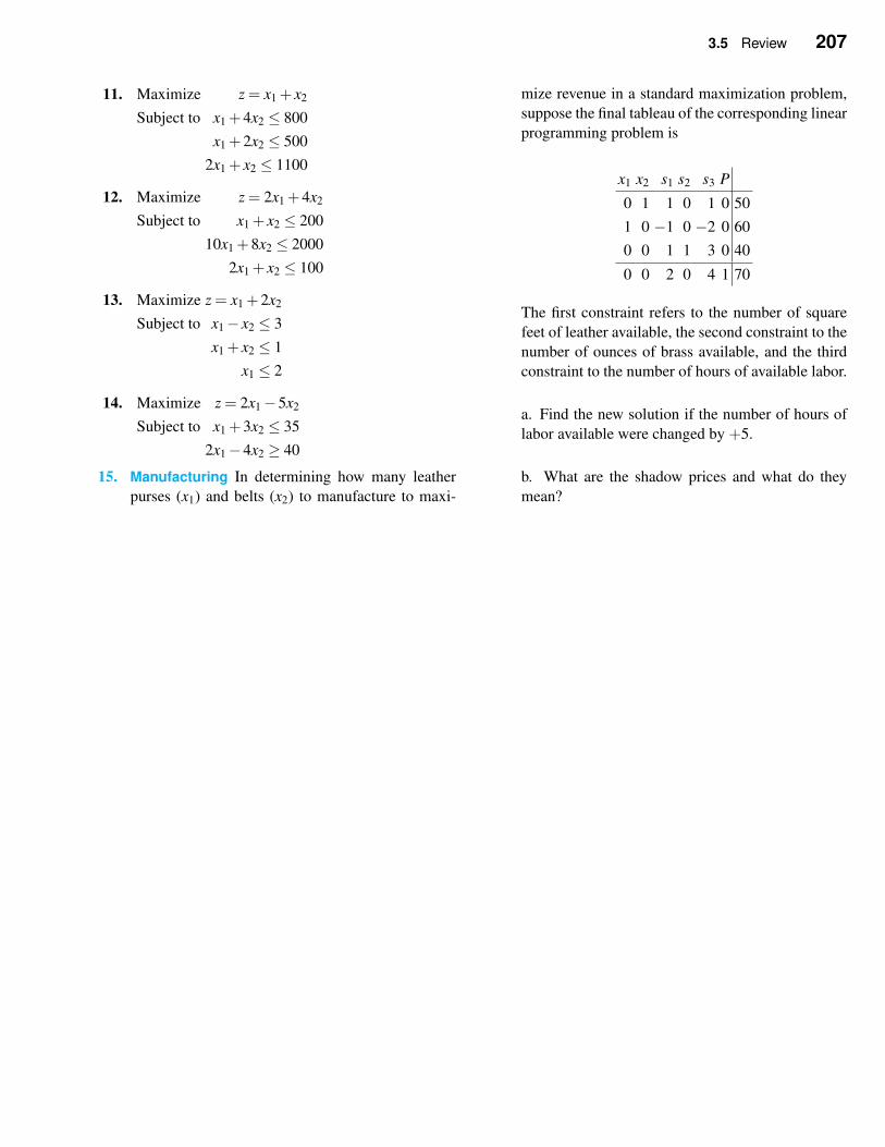
3.5 Review 207
11. Maximize z = x1 + x2
Subject to x1 +4x2 ≤ 800
x1 +2x2 ≤ 500
2x1 + x2 ≤ 1100
12. Maximize z = 2x1 +4x2
Subject to x1 + x2 ≤ 200
10x1 +8x2 ≤ 2000
2x1 + x2 ≤ 100
13. Maximize z = x1 +2x2
Subject to x1− x2 ≤ 3
x1 + x2 ≤ 1
x1 ≤ 2
14. Maximize z = 2x1−5x2
Subject to x1 +3x2 ≤ 35
2x1−4x2 ≥ 40
15. Manufacturing In determining how many leather
purses (x1) and belts (x2) to manufacture to maxi-
mize revenue in a standard maximization problem,
suppose the final tableau of the corresponding linear
programming problem is
x1 x2 s1 s2 s3 P
0 1 1 0 1 0 50
1 0 −1 0 −2 0 60
0 0 1 1 3 0 40
0 0 2 0 4 1 70
The first constraint refers to the number of square
feet of leather available, the second constraint to the
number of ounces of brass available, and the third
constraint to the number of hours of available labor.
a. Find the new solution if the number of hours of
labor available were changed by +5.
b. What are the shadow prices and what do they
mean?
CHAPTER 4Probability
One topic that will be discusssed in the chap-
ter is the expected value of a probability distri-
bution. This is critical to calculating insurance
premiums. On page 239 we see how much an
insurance company will gain, on average, from
insuring at item like this beautiful mint garnet
ring.
4.1 Sample Spaces and Events
Many people have a good idea of the basics of probability. That is, if a fair coin
is flipped, you have an equal chance of a head or a tail showing. However, as we
proceed to study more advanced concepts in probability we need some formal
definitions that will both agree with our intuitive understanding of probability
and allow us to go deeper into topics such as conditional probability.
✧ The Language of Probability
We begin the preliminaries by stating some definitions. It is very important to
have a clear and precise language to discuss probability so pay close attention to
the exact meanings of the terms below.
Experiments and Outcomes
An experiment is an activity that has observable results.
An outcome is the result of the experiment.
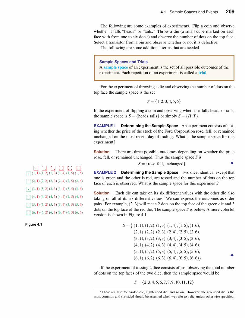
4.1 Sample Spaces and Events 209
The following are some examples of experiments. Flip a coin and observe
whether it falls “heads” or “tails.” Throw a die (a small cube marked on each
face with from one to six dots⋆) and observe the number of dots on the top face.
Select a transistor from a bin and observe whether or not it is defective.
The following are some additional terms that are needed.
Sample Spaces and Trials
A sample space of an experiment is the set of all possible outcomes of the
experiment. Each repetition of an experiment is called a trial.
For the experiment of throwing a die and observing the number of dots on the
top face the sample space is the set
S = {1,2,3,4,5,6}
In the experiment of flipping a coin and observing whether it falls heads or tails,
the sample space is S = {heads, tails} or simply S = {H,T}.
EXAMPLE 1 Determining the Sample Space An experiment consists of not-
ing whether the price of the stock of the Ford Corporation rose, fell, or remained
unchanged on the most recent day of trading. What is the sample space for this
experiment?
Solution There are three possible outcomes depending on whether the price
rose, fell, or remained unchanged. Thus the sample space S is
S = {rose, fell,unchanged} ✦
EXAMPLE 2 Determining the Sample Space Two dice, identical except that
one is green and the other is red, are tossed and the number of dots on the top
face of each is observed. What is the sample space for this experiment?
Solution Each die can take on its six different values with the other die also
taking on all of its six different values. We can express the outcomes as order
pairs. For example, (2, 3) will mean 2 dots on the top face of the green die and 3
dots on the top face of the red die. The sample space S is below. A more colorful
version is shown in Figure 4.1.
Figure 4.1 S = { (1,1),(1,2),(1,3),(1,4),(1,5),(1,6),(2,1),(2,2),(2,3),(2,4),(2,5),(2,6),
(3,1),(3,2),(3,3),(3,4),(3,5),(3,6),
(4,1),(4,2),(4,3),(4,4),(4,5),(4,6),
(5,1),(5,2),(5,3),(5,4),(5,5),(5,6),
(6,1),(6,2),(6,3),(6,4),(6,5),(6,6)} ✦
If the experiment of tossing 2 dice consists of just observing the total number
of dots on the top faces of the two dice, then the sample space would be
S = {2,3,4,5,6,7,8,9,10,11,12}
⋆There are also four-sided die, eight-sided die, and so on. However, the six-sided die is the
most common and six-sided should be assumed when we refer to a die, unless otherwise specified.
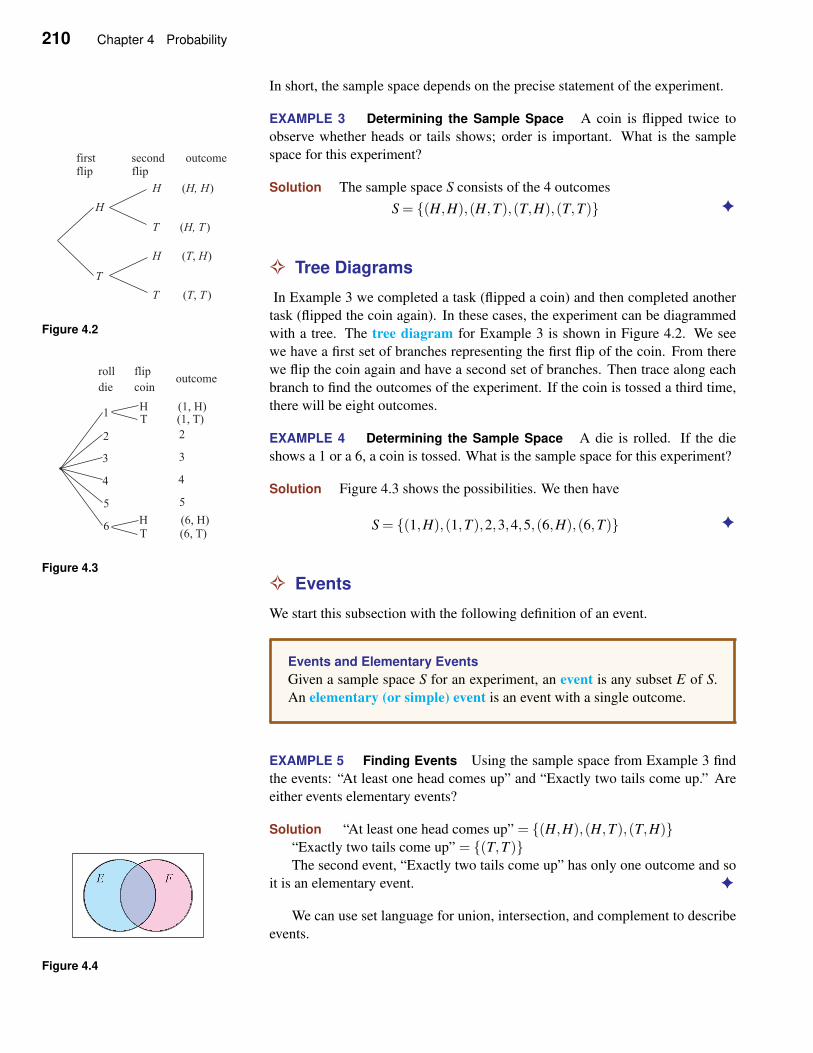
210 Chapter 4 Probability
In short, the sample space depends on the precise statement of the experiment.
EXAMPLE 3 Determining the Sample Space A coin is flipped twice to
observe whether heads or tails shows; order is important. What is the sample
space for this experiment?
Solution The sample space S consists of the 4 outcomes
S = {(H,H),(H,T ),(T,H),(T,T )} ✦
✧ Tree Diagrams
In Example 3 we completed a task (flipped a coin) and then completed another
Figure 4.2task (flipped the coin again). In these cases, the experiment can be diagrammed
with a tree. The tree diagram for Example 3 is shown in Figure 4.2. We see
we have a first set of branches representing the first flip of the coin. From there
we flip the coin again and have a second set of branches. Then trace along each
branch to find the outcomes of the experiment. If the coin is tossed a third time,
there will be eight outcomes.
EXAMPLE 4 Determining the Sample Space A die is rolled. If the die
shows a 1 or a 6, a coin is tossed. What is the sample space for this experiment?
Solution Figure 4.3 shows the possibilities. We then have
Figure 4.3
S = {(1,H),(1,T ),2,3,4,5,(6,H),(6,T)} ✦
✧ Events
We start this subsection with the following definition of an event.
Events and Elementary Events
Given a sample space S for an experiment, an event is any subset E of S.
An elementary (or simple) event is an event with a single outcome.
EXAMPLE 5 Finding Events Using the sample space from Example 3 find
the events: “At least one head comes up” and “Exactly two tails come up.” Are
either events elementary events?
Solution “At least one head comes up” = {(H,H),(H,T ),(T,H)}“Exactly two tails come up” = {(T,T )}The second event, “Exactly two tails come up” has only one outcome and so
it is an elementary event. ✦
We can use set language for union, intersection, and complement to describe
events.
Figure 4.4
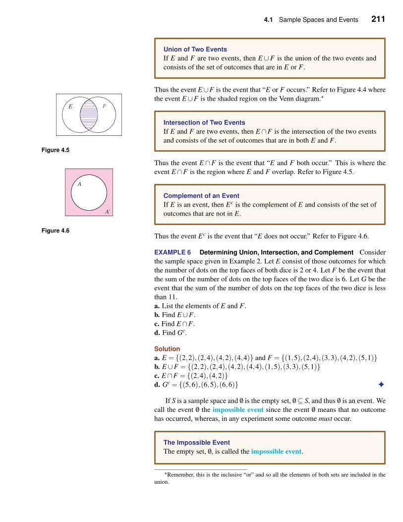
4.1 Sample Spaces and Events 211
Union of Two Events
If E and F are two events, then E ∪F is the union of the two events and
consists of the set of outcomes that are in E or F .
Thus the event E∪F is the event that “E or F occurs.” Refer to Figure 4.4 where
the event E ∪F is the shaded region on the Venn diagram.⋆
E F
Figure 4.5
Intersection of Two Events
If E and F are two events, then E ∩F is the intersection of the two events
and consists of the set of outcomes that are in both E and F .
Thus the event E ∩F is the event that “E and F both occur.” This is where the
event E ∩F is the region where E and F overlap. Refer to Figure 4.5.
A
Ac
Figure 4.6
Complement of an Event
If E is an event, then Ec is the complement of E and consists of the set of
outcomes that are not in E.
Thus the event Ec is the event that “E does not occur.” Refer to Figure 4.6.
EXAMPLE 6 Determining Union, Intersection, and Complement Consider
the sample space given in Example 2. Let E consist of those outcomes for which
the number of dots on the top faces of both dice is 2 or 4. Let F be the event that
the sum of the number of dots on the top faces of the two dice is 6. Let G be the
event that the sum of the number of dots on the top faces of the two dice is less
than 11.
a. List the elements of E and F .
b. Find E ∪F .
c. Find E ∩F .
d. Find Gc.
Solution
a. E = {(2,2),(2,4),(4,2),(4,4)} and F = {(1,5),(2,4),(3,3),(4,2),(5,1)}b. E ∪F = {(2,2),(2,4),(4,2),(4,4),(1,5),(3,3),(5,1)}c. E ∩F = {(2,4),(4,2)}d. Gc = {(5,6),(6,5),(6,6)} ✦
If S is a sample space and /0 is the empty set, /0⊆ S, and thus /0 is an event. We
call the event /0 the impossible event since the event /0 means that no outcome
has occurred, whereas, in any experiment some outcome must occur.
The Impossible Event
The empty set, /0, is called the impossible event.
⋆Remember, this is the inclusive “or” and so all the elements of both sets are included in the
union.
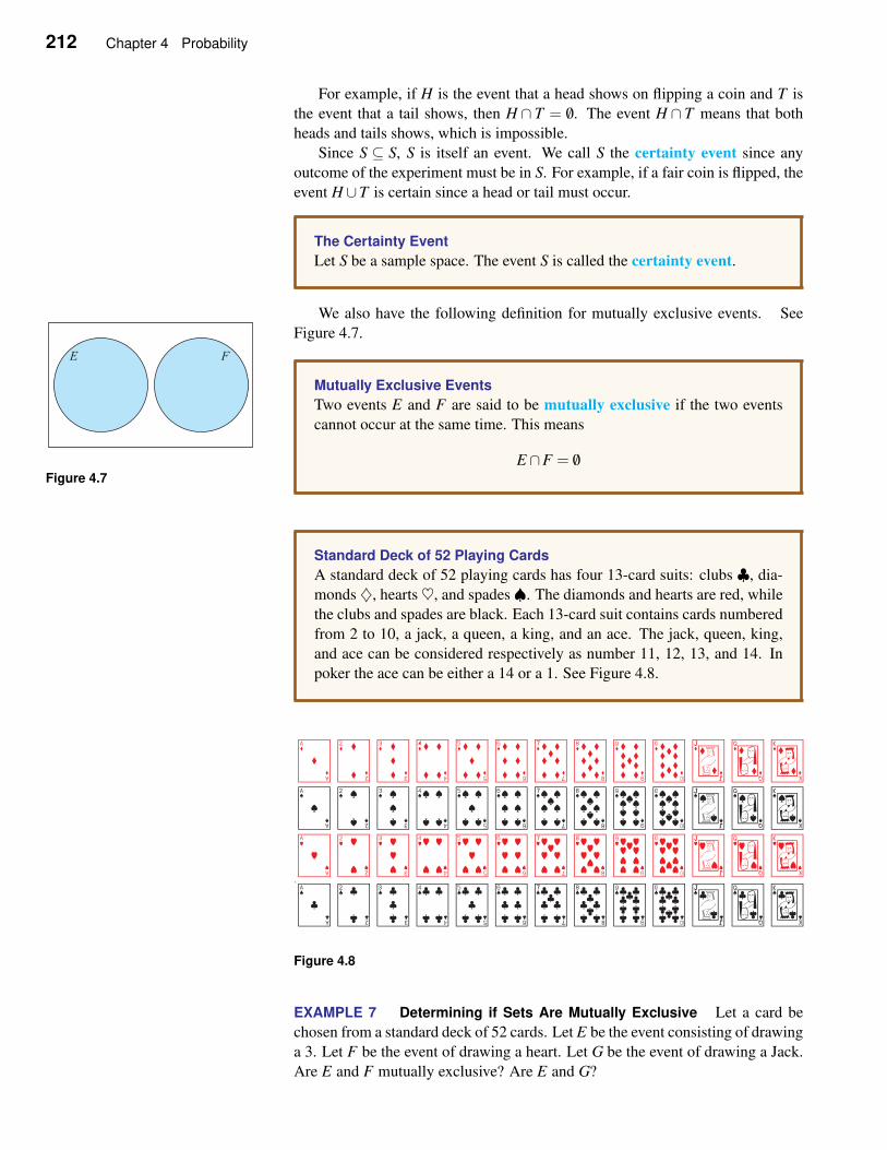
212 Chapter 4 Probability
For example, if H is the event that a head shows on flipping a coin and T is
the event that a tail shows, then H ∩ T = /0. The event H ∩ T means that both
heads and tails shows, which is impossible.
Since S ⊆ S, S is itself an event. We call S the certainty event since any
outcome of the experiment must be in S. For example, if a fair coin is flipped, the
event H ∪T is certain since a head or tail must occur.
The Certainty Event
Let S be a sample space. The event S is called the certainty event.
We also have the following definition for mutually exclusive events. See
Figure 4.7
Figure 4.7.
Mutually Exclusive Events
Two events E and F are said to be mutually exclusive if the two events
cannot occur at the same time. This means
E ∩F = /0
Standard Deck of 52 Playing Cards
A standard deck of 52 playing cards has four 13-card suits: clubs ♣, dia-
monds♦, hearts♥, and spades♠. The diamonds and hearts are red, while
the clubs and spades are black. Each 13-card suit contains cards numbered
from 2 to 10, a jack, a queen, a king, and an ace. The jack, queen, king,
and ace can be considered respectively as number 11, 12, 13, and 14. In
poker the ace can be either a 14 or a 1. See Figure 4.8.
Figure 4.8
EXAMPLE 7 Determining if Sets Are Mutually Exclusive Let a card be
chosen from a standard deck of 52 cards. Let E be the event consisting of drawing
a 3. Let F be the event of drawing a heart. Let G be the event of drawing a Jack.
Are E and F mutually exclusive? Are E and G?
4.1 Sample Spaces and Events 213
Solution Since E ∩F is the event that the card is a 3 and is a heart,
E ∩F = {3♥} 6= /0
and so these events are not mutually exclusive. The event E ∩G is the event that
the card is a 3 and a jack, so
E ∩G = /0
therefore E and G are mutually exclusive. ✦
✧ Continuous Sample Spaces
In all the previous examples we were able to list each outcome in the sample
space, even if the list is rather long. But consider the outcomes of an experiment
where the time spent running a race is measured. Depending on how the time is
measured, an outcome could be 36 seconds or 36.0032 seconds. The values of
the outcomes are not restricted to whole numbers and so the sample space must
be described, rather than listed. In the case of the race we could say S = {t|t ≥0, t in seconds}. Then the event E that a person takes less than 35 seconds to run
the race would be written E = {t|t < 35 seconds}.
EXAMPLE 8 Weighing Oranges At a farmer’s market there is a display of
fresh oranges. The oranges are carefully weighed. What is a sample space for
this experiment? Describe the event that a orange weighs 100 grams or more.
Describe the event that a orange weighs between 200 and 250 grams.
Solution Since the weight of the orange can be any positive number,
S = {w|w > 0,w in grams}
Note that w = 0 is not included as if the weight was zero there would be no
orange! The event that an orange weighs 100 grams or more is
E = {w|w≥ 100,w in grams}
Here note that we use ≥, not > as the value of exactly 100 grams needs to be
included. The event that the orange weighs between 200 and 250 grams is
F = {w|200 < w < 250,w in grams}
where strict inequalities are used as the weight is between those values. ✦
Self-Help Exercises 4.1
1. Two tetrahedrons (4 sided), each with equal sides
numbered from 1 to 4, are identical except that one
is red and the other green. If the two tetrahedrons
are tossed and the number on the bottom face of
each is observed, what is the sample space for this
experiment?
2. Consider the sample space given in the previous ex-
ercise. Let E consist of those outcomes for which
both (tetrahedron) dice show an odd number. Let
214 Chapter 4 Probability
F be the event that the sum of the two numbers on
these dice is 5. Let G be the event that the sum of
the two numbers is less than 7.
a. List the elements of E and F .
b. Find E ∩F .
c. Find E ∪F .
d. Find Gc.
3. A hospital carefully measures the length of every
baby born. What is a sample space for this experi-
ment? Describe the events
a. the baby is longer than 22 inches.
b. the baby is 20 inches or shorter.
c. the baby is between 19.5 and 21 inches long.
4.1 Exercises
1. Let S = {a,b,c} be a sample space. Find all the
events.
2. Let the sample space be S = {a,b,c,d}. How many
events are there?
3. A coin is flipped three times, and heads or tails is
observed after each flip. What is the sample space?
Indicate the outcomes in the event “at least 2 heads
are observed.”
4. A coin is flipped, and it is noted whether heads or
tails show. A die is tossed, and the number on the
top face is noted. What is the sample space of this
experiment?
5. A coin is flipped three times. If heads show, one is
written down. If tails show, zero is written down.
What is the sample space for this experiment? Indi-
cate the outcomes if “one is observed at least twice.”
6. Two tetrahedrons (4 sided), each with equal sides
numbered from 1 to 4, are identical except that one
is red and the other green. If the two tetrahedrons
are tossed and the number on the bottom face of
each is observed, indicate the outcomes in the event
“the sum of the numbers is 4.”
7. An urn holds 10 identical balls except that 1 is
white, 4 are black, and 5 are red. An experiment
consists of selecting a ball from the urn and observ-
ing its color. What is a sample space for this exper-
iment? Indicate the outcomes in the event “the ball
is not white.”
8. For the urn in Exercise 7, an experiment consists of
selecting 2 balls in succession without replacement
and observing the color of each of the balls. What
is the sample space of this experiment? Indicate the
outcomes of the event “no ball is white.”
9. Ann, Bubba, Carlos, David, and Elvira are up for
promotion. Their boss must select three people from
this group of five to be promoted. What is the
sample space? Indicate the outcomes of the event
“Bubba is selected.”
10. A restaurant offers six side dishes: rice, macaroni,
potatoes, corn, broccoli, and carrots. A customer
must select two different side dishes for his dinner.
What is the sample space? List the outcomes of the
event “Corn is selected.”
11. An experiment consists of selecting a digit from
the number 112964333 and observing it. What is
a sample space for this experiment? Indicate the
outcomes in the event that “an even digit.”
12. An experiment consists of selecting a letter from the
word CONNECTICUT and observing it. What is a
sample space for this experiment? Indicate the out-
comes of the event “a vowel is selected.”
13. An inspector selects 10 transistors from the produc-
tion line and notes how many are defective.
a. Determine the sample space.
b. Find the outcomes in the set corresponding to
the event E “at least 6 are defective.”
c. Find the outcomes in the set corresponding to
the event F “at most 4 are defective.”
d. Find the sets E ∪F , E ∩F , Ec, E ∩Fc, Ec∩Fc.
e. Find all pairs of sets among the nonempty ones
listed in part (d) that are mutually exclusive.
14. A survey indicates first whether a person is in the
lower income group (L), middle income group (M),
or upper income group (U), and second which of
these groups the father of the person is in.
a. Determine the sample space using the letters L,
M, and U .
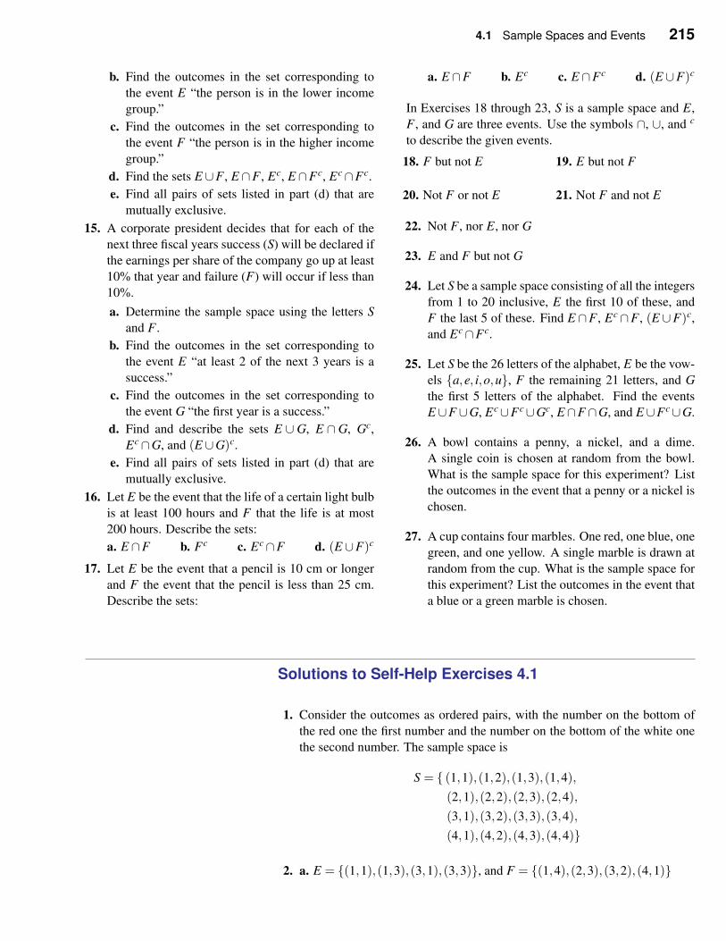
4.1 Sample Spaces and Events 215
b. Find the outcomes in the set corresponding to
the event E “the person is in the lower income
group.”
c. Find the outcomes in the set corresponding to
the event F “the person is in the higher income
group.”
d. Find the sets E ∪F , E ∩F , Ec, E ∩Fc, Ec∩Fc.
e. Find all pairs of sets listed in part (d) that are
mutually exclusive.
15. A corporate president decides that for each of the
next three fiscal years success (S) will be declared if
the earnings per share of the company go up at least
10% that year and failure (F) will occur if less than
10%.
a. Determine the sample space using the letters S
and F .
b. Find the outcomes in the set corresponding to
the event E “at least 2 of the next 3 years is a
success.”
c. Find the outcomes in the set corresponding to
the event G “the first year is a success.”
d. Find and describe the sets E ∪G, E ∩G, Gc,
Ec∩G, and (E ∪G)c.
e. Find all pairs of sets listed in part (d) that are
mutually exclusive.
16. Let E be the event that the life of a certain light bulb
is at least 100 hours and F that the life is at most
200 hours. Describe the sets:
a. E ∩F b. Fc c. Ec∩F d. (E ∪F)c
17. Let E be the event that a pencil is 10 cm or longer
and F the event that the pencil is less than 25 cm.
Describe the sets:
a. E ∩F b. Ec c. E ∩Fc d. (E ∪F)c
In Exercises 18 through 23, S is a sample space and E,
F , and G are three events. Use the symbols ∩, ∪, and c
to describe the given events.
18. F but not E 19. E but not F
20. Not F or not E 21. Not F and not E
22. Not F , nor E, nor G
23. E and F but not G
24. Let S be a sample space consisting of all the integers
from 1 to 20 inclusive, E the first 10 of these, and
F the last 5 of these. Find E ∩F , Ec∩F , (E ∪F)c,
and Ec∩Fc.
25. Let S be the 26 letters of the alphabet, E be the vow-
els {a,e, i,o,u}, F the remaining 21 letters, and G
the first 5 letters of the alphabet. Find the events
E∪F ∪G, Ec∪Fc∪Gc, E∩F ∩G, and E∪Fc∪G.
26. A bowl contains a penny, a nickel, and a dime.
A single coin is chosen at random from the bowl.
What is the sample space for this experiment? List
the outcomes in the event that a penny or a nickel is
chosen.
27. A cup contains four marbles. One red, one blue, one
green, and one yellow. A single marble is drawn at
random from the cup. What is the sample space for
this experiment? List the outcomes in the event that
a blue or a green marble is chosen.
Solutions to Self-Help Exercises 4.1
1. Consider the outcomes as ordered pairs, with the number on the bottom of
the red one the first number and the number on the bottom of the white one
the second number. The sample space is
S = { (1,1),(1,2),(1,3),(1,4),(2,1),(2,2),(2,3),(2,4),
(3,1),(3,2),(3,3),(3,4),
(4,1),(4,2),(4,3),(4,4)}
2. a. E = {(1,1),(1,3),(3,1),(3,3)}, and F = {(1,4),(2,3),(3,2),(4,1)}
216 Chapter 4 Probability
b. E ∩F = /0
c. E ∪F = {(1,1),(1,3),(3,1),(3,3),(1,4),(2,3),(3,2),(4,1)}d. Gc = {(3,4),(4,3),(4,4)}
3. Since the baby can be any length greater than zero, the sample space is
S = {x|x > 0,x in inches}
a. E = {x|x > 22,x in inches}b. F = {x|x≤ 20,x in inches}c. G = {x|19.5 < x < 21,x in inches}
4.2 Basics of Probability
✧ Introduction to Probability
We first consider sample spaces for which the outcomes (elementary events) are
equally likely. For example, a head or tail is equally likely to come up on a flip of
a fair coin. Any of the six numbers on a fair die is equally likely to come up on
a roll. We will refer to a sample space S whose individual elementary events are
equally likely as a uniform sample space. We then give the following definition
of the probability of any event in a uniform sample space.
HISTORICAL NOTE
The Beginnings of
Probability
In 1654 the famous mathematician
Blaise Pascal had a friend,
Chevalier de Mere, a member of
the French nobility and a gambler,
who wanted to adjust gambling
stakes so that he would be assured
of winning if he played long
enough. This gambler raised
questions with Pascal such as the
following: In eight throws of a die a
player attempts to throw a one, but
after three unsuccessful trials the
game is interrupted. How should
he be compensated? Pascal wrote
to a leading mathematician of that
day, Pierre de Fermat
(1601–1665), about these
problems, and their resulting
correspondence represents the
beginnings of the modern theory of
mathematical probability.
Probability of an Event in a Uniform Sample Space
If S is a finite uniform sample space and E is any event, then the probabil-
ity of E, P(E), is given by
P(E) =Number of elements in E
Number of elements in S=
n(E)
n(S)
EXAMPLE 1 Probability for a Single Die Suppose a fair die is rolled and
the sample space is S = {1,2,3,4,5,6}. Determine the probability of each of the
following events.
a. The die shows an odd number.
b. The die shows the number 9.
c. The die shows a number less than 8.
Solution a. We have E = {1,3,5}. Then
P(E) =n(E)
n(S)=
3
6=
1
2
b. The event F that the die shows a 9 is the impossible event. So n(F) = 0 and
P(F) =n(F)
n(S)=
0
6= 0
4.2 Basics of Probability 217
c. The event G that the die shows a number less than 8 is just the certainty event.
So G = {1,2,3,4,5,6}= S and
P(G) =n(G)
n(S)=
6
6= 1 ✦
EXAMPLE 2 Probability for a Single Card Suppose a single card is randomly
drawn from a standard 52-card deck. Determine the probability of each of the
following events.
a. A king is drawn.
b. A heart is drawn.
Solution a. The event is E = { K♦, K♥, K♠, K♣}. So,
P(E) =n(E)
n(S)=
4
52=
1
13
b. The event F contains 13 hearts. So
P(F) =n(F)
n(S)=
13
52=
1
4✦
EXAMPLE 3 Probability for Transistors A bin contains 15 identical (to the
eye) transistors except that 6 are defective and 9 are not. What is the probability
that a transistor selected at random is defective?
Solution Let us denote the set S to be the set of all 15 transistors and the set E
to be the set of defective transistors. Then,
P(E) =n(E)
n(S)=
6
15=
2
5✦
EXAMPLE 4 Probability for Two Coin Flips A fair coin is flipped twice to
observe whether heads or tails shows; order is important. What is the probability
that tails occurs both times?
Solution The sample space S consists of the 4 outcomes
S = {(H,H),(H,T ),(T,H),(T,T )}
Since we are using a fair coin, each of the individual four elementary events are
equally likely. The set E that tails occurs both times is E = {(T,T )} and contains
one element. We have
P(E) =n(E)
n(S)=
1
4✦
✧ Empirical Probability
HISTORICAL NOTE
The Beginnings of
Empirical Probability
Empirical probability began with
the emergence of insurance
companies. Insurance seems to
have been originally used to
protect merchant vessels and was
in use even in Roman times. The
first marine insurance companies
began in Italy and Holland in the
14th century and spread to other
countries by the 16th century. In
fact, the famous Lloyd’s of London
was founded in the late 1600s. The
first life insurance seems to have
been written in the late 16th
century in Europe. All of these
companies naturally needed to
know with what the likelihood of
certain events would occur. The
empirical probabilities were
determined by collecting data over
long periods of time.
A very important type of problem that arises every day in business and science is
to find a practical way to estimate the likelihood of certain events. For example,
a food company may seek a practical method of estimating the likelihood that a
new type of candy will be enjoyed by consumers. The most obvious procedure for
the company to follow is to randomly select a consumer, have the consumer taste
the candy, and then record the result. This should be repeated many times and the
final totals tabulated to give the fraction of tested consumers who enjoy the candy.
218 Chapter 4 Probability
This fraction is then a practical estimate of the likelihood that all consumers will
enjoy this candy. We refer to this fraction or number as empirical probability.
The London merchant John Graunt (1620–1674) with the publication of Nat-
ural and Political Observations Made upon the Bills of Mortality in 1662 seems
to have been the first person to have gathered data on mortality rates and deter-
mined empirical probabilities from them. The data were extremely difficult to
obtain. His then-famous London Life Table is reproduced below, showing the
number of survivors through certain ages per 100 people.
Age 0 6 16 26 36 46 56 66 76
Survivors 100 64 40 25 16 10 6 3 1
EXAMPLE 5 Finding Empirical Probability Using the London Life Table,
find the empirical probability of a randomly chosen person living in London in
the first half of the 17th century surviving until age 46.
Solution In the London Life Table N = 100. If E is the event “survive to
age 46,” then according to the table the corresponding number is 10. Thus, the
empirical probability of people living in London at that time surviving until age
46 was 10/100 = 0.1. ✦
Consider now a poorly made die purchased at a discount store. Dice are made
by drilling holes in the sides and then backfilling. Cheap dice are, of course, not
carefully backfilled. So when a lot of holes are made in a face, such as for a side
with 6, and they are not carefully backfilled, that side will not be quite as heavy
as the others. Thus a 6 will tend to come up more often on the top. Even a die
taken from a craps table in Las Vegas, where the dice are of very high quality,
will have some tiny imbalance.
EXAMPLE 6 Finding Empirical Probability A die with 6 sides numbered
from 1 to 6, such as used in the game of craps, is suspected to be somewhat
lopsided. A laboratory has tossed this die 1000 times and obtained the results
shown in the table. Find the empirical probability that a 2 will occur and the
probability that a 6 will occur.
Outcome 1 2 3 4 5 6
Number Observed 161 179 148 177 210 125
Solution The total number observed is 1000. The number observed for the 2
and 6, respectively is 179 and 125. So dividing these numbers by 1000 gives
P(2) = 179/1000 = 0.179
P(6) = 125/1000 = 0.125 ✦
4.2 Basics of Probability 219
CONNECTION
Frederick Mosteller and the
Dice Experiment
Frederick Mosteller has been president of the American Association for the
Advancement of Science, the Institute of Mathematical Statistics, and the
American Statistical Association. He once decided that “It would be nice
to see if the actual outcome of a real person tossing real dice would match
up with the theory.” He then engaged Willard H. Longcor to buy some
dice, toss them, and keep careful records of the outcomes. Mr. Longcor
then tossed the dice on his floor at home so that the dice would bounce on
the floor and then up against the wall and then land back on the floor. After
doing this several thousand times his wife became troubled by the noise.
He then placed a rug on the floor and on the wall, and then proceeded
to quietly toss his dice millions of times, keeping careful records of the
outcomes. In fact, he was so careful and responsible about his task, that
he threw away his data on the first 100,000 tosses, since he had a nagging
worry that he might have made some mistake keeping perfect track.
✧ Probability Distribution Tables
A probability distribution table is a useful way to display probability data for
an experiment. In a probability distribution table there is one column (or row) for
the events that take place and one column (or row) for the probability of the event.
The events chosen must be mutually exclusive and therefore the total probability
will add to 1. This is best demonstrated through an example.
EXAMPLE 7 Flipping a Coin Twice Write the probability distribution table
for the number of heads when a coin is flipped twice.
Solution Recall from Example 4 that the uniform sample space is S ={(H,H),(H,T ),(T,H),(T,T )}. Next, we are asked to organize the events by
the number of heads, so we will have three events
E1 = {(H,H)} with two heads and a probability of 1/4,
E2 = {(H,T ),(T,H)} with exactly one head and a probability of 2/4
E3 = {(T,T )} with zero heads and a probability of 1/4.
This is shown in the table on the left. ✦
Event Probability
2 heads 1/4
1 head 1/2
0 heads 1/4 Note how the list of events covered all the possibilities for the number of
heads and that the events are all mutually exclusive. You can’t have exactly
two heads and exactly one head at the same time! Next see that the sum of the
probabilities is equal to one. This will always be the case when your probability
distribution table is correct.
EXAMPLE 8 Sum of the Numbers for Two Dice Two fair dice are rolled.
Find the probability distribution table for the sum of the numbers shown upper-
most.
Solution Recall the uniform sample space in Example 2 of the last section for
rolling two dice. We see the smallest sum is 2 from the roll (1,1) and the largest
sum is 12 from the roll (6,6). Count the number of outcomes in each event to find
the probability:
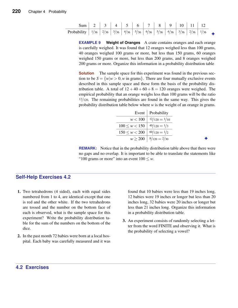
220 Chapter 4 Probability
Sum 2 3 4 5 6 7 8 9 10 11 12
Probability 1/36 2/36 3/36 4/36 5/36 6/36 5/36 4/36 3/36 2/36 1/36 ✦
EXAMPLE 9 Weight of Oranges A crate contains oranges and each orange
is carefully weighed. It was found that 12 oranges weighed less than 100 grams,
40 oranges weighed 100 grams or more, but less than 150 grams, 60 oranges
weighed 150 grams or more, but less than 200 grams, and 8 oranges weighed
200 grams or more. Organize this information in a probability distribution table
Solution The sample space for this experiment was found in the previous sec-
tion to be S = {w|w > 0,w in grams}. There are four mutually exclusive events
described in this sample space and these form the basis of the probability dis-
tribution table. A total of 12+ 40+ 60+ 8 = 120 oranges were weighed. The
empirical probability that an orange weighs less than 100 grams will be the ratio12/120. The remaining probabilities are found in the same way. This gives the
probability distribution table below where w is the weight of an orange in grams.
Event Probability
w < 100 12/120 = 1/10
100≤ w < 150 40/120 = 1/3
150≤ w < 200 60/120 = 1/2
w≥ 200 8/120 = 2/30 ✦
REMARK: Notice that in the probability distribution table above that there were
no gaps and no overlap. It is important to be able to translate the statements like
“100 grams or more” into an event 100≤ w.
Self-Help Exercises 4.2
1. Two tetrahedrons (4 sided), each with equal sides
numbered from 1 to 4, are identical except that one
is red and the other white. If the two tetrahedrons
are tossed and the number on the bottom face of
each is observed, what is the sample space for this
experiment? Write the probability distribution ta-
ble for the sum of the numbers on the bottom of the
dice.
2. In the past month 72 babies were born at a local hos-
pital. Each baby was carefully measured and it was
found that 10 babies were less than 19 inches long,
12 babies were 19 inches or longer but less than 20
inches long, 32 babies were 20 inches or longer but
less than 21 inches long. Organize this information
in a probability distribution table.
3. An experiment consists of randomly selecting a let-
ter from the word FINITE and observing it. What is
the probability of selecting a vowel?
4.2 Exercises
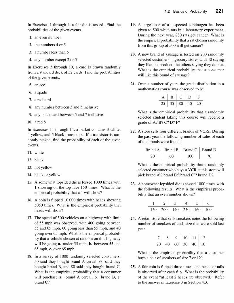
4.2 Basics of Probability 221
In Exercises 1 through 4, a fair die is tossed. Find the
probabilities of the given events.
1. an even number
2. the numbers 4 or 5
3. a number less than 5
4. any number except 2 or 5
In Exercises 5 through 10, a card is drawn randomly
from a standard deck of 52 cards. Find the probabilities
of the given events.
5. an ace
6. a spade
7. a red card
8. any number between 3 and 5 inclusive
9. any black card between 5 and 7 inclusive
10. a red 8
In Exercises 11 through 14, a basket contains 3 white,
4 yellow, and 5 black transistors. If a transistor is ran-
domly picked, find the probability of each of the given
events.
11. white
12. black
13. not yellow
14. black or yellow
15. A somewhat lopsided die is tossed 1000 times with
1 showing on the top face 150 times. What is the
empirical probability that a 1 will show?
16. A coin is flipped 10,000 times with heads showing
5050 times. What is the empirical probability that
heads will show?
17. The speed of 500 vehicles on a highway with limit
of 55 mph was observed, with 400 going between
55 and 65 mph, 60 going less than 55 mph, and 40
going over 65 mph. What is the empirical probabil-
ity that a vehicle chosen at random on this highway
will be going a. under 55 mph, b. between 55 and
65 mph, c. over 65 mph.
18. In a survey of 1000 randomly selected consumers,
50 said they bought brand A cereal, 60 said they
bought brand B, and 80 said they bought brand C.
What is the empirical probability that a consumer
will purchase a. brand A cereal, b. brand B, c.
brand C?
19. A large dose of a suspected carcinogen has been
given to 500 white rats in a laboratory experiment.
During the next year, 280 rats get cancer. What is
the empirical probability that a rat chosen randomly
from this group of 500 will get cancer?
20. A new brand of sausage is tested on 200 randomly
selected customers in grocery stores with 40 saying
they like the product, the others saying they do not.
What is the empirical probability that a consumer
will like this brand of sausage?
21. Over a number of years the grade distribution in a
mathematics course was observed to be
A B C D F
25 35 80 40 20
What is the empirical probability that a randomly
selected student taking this course will receive a
grade of A? B? C? D? F?
22. A store sells four different brands of VCRs. During
the past year the following number of sales of each
of the brands were found.
Brand A Brand B Brand C Brand D
20 60 100 70
What is the empirical probability that a randomly
selected customer who buys a VCR at this store will
pick brand A’? brand B:’ brand C’? brand D?
23. A somewhat lopsided die is tossed 1000 times with
the following results. What is the empirical proba-
bility that an even number shows?
1 2 3 4 5 6
150 200 140 250 160 100
24. A retail store that sells sneakers notes the following
number of sneakers of each size that were sold last
year.
7 8 9 10 11 12
20 40 60 30 40 10
What is the empirical probability that a customer
buys a pair of sneakers of size 7 or 12?
25. A fair coin is flipped three times, and heads or tails
is observed after each flip. What is the probability
of the event “at least 2 heads are observed.” Refer
to the answer in Exercise 3 in Section 4.3.
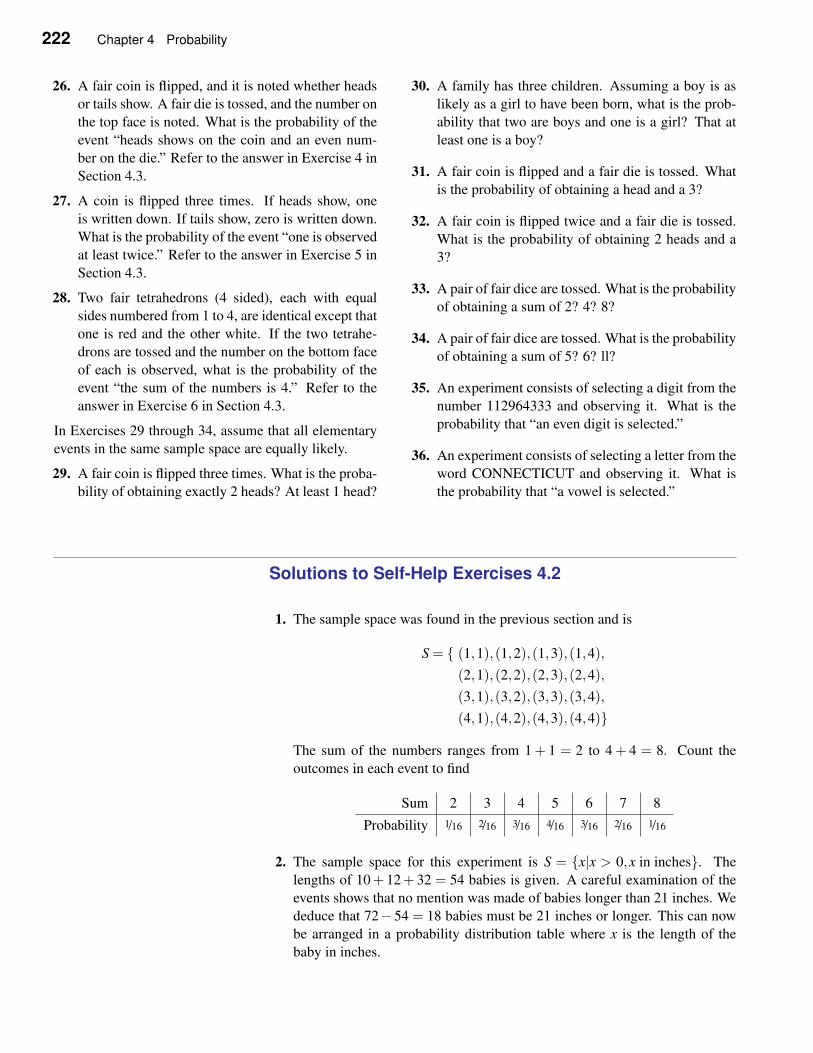
222 Chapter 4 Probability
26. A fair coin is flipped, and it is noted whether heads
or tails show. A fair die is tossed, and the number on
the top face is noted. What is the probability of the
event “heads shows on the coin and an even num-
ber on the die.” Refer to the answer in Exercise 4 in
Section 4.3.
27. A coin is flipped three times. If heads show, one
is written down. If tails show, zero is written down.
What is the probability of the event “one is observed
at least twice.” Refer to the answer in Exercise 5 in
Section 4.3.
28. Two fair tetrahedrons (4 sided), each with equal
sides numbered from 1 to 4, are identical except that
one is red and the other white. If the two tetrahe-
drons are tossed and the number on the bottom face
of each is observed, what is the probability of the
event “the sum of the numbers is 4.” Refer to the
answer in Exercise 6 in Section 4.3.
In Exercises 29 through 34, assume that all elementary
events in the same sample space are equally likely.
29. A fair coin is flipped three times. What is the proba-
bility of obtaining exactly 2 heads? At least 1 head?
30. A family has three children. Assuming a boy is as
likely as a girl to have been born, what is the prob-
ability that two are boys and one is a girl? That at
least one is a boy?
31. A fair coin is flipped and a fair die is tossed. What
is the probability of obtaining a head and a 3?
32. A fair coin is flipped twice and a fair die is tossed.
What is the probability of obtaining 2 heads and a
3?
33. A pair of fair dice are tossed. What is the probability
of obtaining a sum of 2? 4? 8?
34. A pair of fair dice are tossed. What is the probability
of obtaining a sum of 5? 6? ll?
35. An experiment consists of selecting a digit from the
number 112964333 and observing it. What is the
probability that “an even digit is selected.”
36. An experiment consists of selecting a letter from the
word CONNECTICUT and observing it. What is
the probability that “a vowel is selected.”
Solutions to Self-Help Exercises 4.2
1. The sample space was found in the previous section and is
S = { (1,1),(1,2),(1,3),(1,4),(2,1),(2,2),(2,3),(2,4),
(3,1),(3,2),(3,3),(3,4),
(4,1),(4,2),(4,3),(4,4)}
The sum of the numbers ranges from 1+ 1 = 2 to 4+ 4 = 8. Count the
outcomes in each event to find
Sum 2 3 4 5 6 7 8
Probability 1/16 2/16 3/16 4/16 3/16 2/16 1/16
2. The sample space for this experiment is S = {x|x > 0,x in inches}. The
lengths of 10+ 12+ 32 = 54 babies is given. A careful examination of the
events shows that no mention was made of babies longer than 21 inches. We
deduce that 72−54 = 18 babies must be 21 inches or longer. This can now
be arranged in a probability distribution table where x is the length of the
baby in inches.
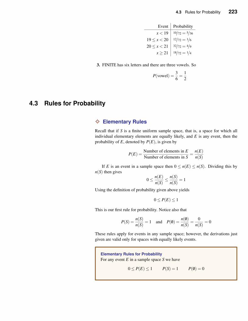
4.3 Rules for Probability 223
Event Probability
x < 19 10/72 = 5/36
19≤ x < 20 12/72 = 1/6
20≤ x < 21 32/72 = 4/9
x≥ 21 18/72 = 1/4
3. FINITE has six letters and there are three vowels. So
P(vowel) =3
6=
1
2
4.3 Rules for Probability
✧ Elementary Rules
Recall that if S is a finite uniform sample space, that is, a space for which all
individual elementary elements are equally likely, and E is any event, then the
probability of E, denoted by P(E), is given by
P(E) =Number of elements in E
Number of elements in S=
n(E)
n(S)
If E is an event in a sample space then 0 ≤ n(E) ≤ n(S). Dividing this by
n(S) then gives
0≤ n(E)
n(S)≤ n(S)
n(S)= 1
Using the definition of probability given above yields
0≤ P(E)≤ 1
This is our first rule for probability. Notice also that
P(S) =n(S)
n(S)= 1 and P( /0) =
n( /0)
n(S)=
0
n(S)= 0
These rules apply for events in any sample space; however, the derivations just
given are valid only for spaces with equally likely events.
Elementary Rules for Probability
For any event E in a sample space S we have
0≤ P(E)≤ 1 P(S) = 1 P( /0) = 0
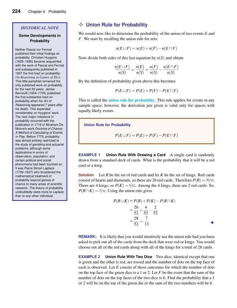
224 Chapter 4 Probability
✧ Union Rule for Probability
We would now like to determine the probability of the union of two events E and
F . We start by recalling the union rule for sets:
n(E ∪F) = n(E)+n(F)−n(E ∩F)
Now divide both sides of this last equation by n(S) and obtain
n(E ∪F)
n(S)=
n(E)
n(S)+
n(F)
n(S)− n(E ∩F)
n(S)
By the definition of probability given above this becomes
P(E ∪F) = P(E)+P(F)−P(E ∩F)
This is called the union rule for probability. This rule applies for events in any
sample space; however, the derivation just given is valid only for spaces with
equally likely events.
HISTORICAL NOTE
Some Developments in
Probability
Neither Pascal nor Fermat
published their initial findings on
probability. Christian Huygens
(1629–1695) became acquainted
with the work of Pascal and Fermat
and subsequently published in
1657 the first tract on probability:
On Reasoning in Games of Dice.
This little pamphlet remained the
only published work on probability
for the next 50 years. James
Bernoulli (1654–1705) published
the first substantial tract on
probability when his Art of
Reasoning appeared 7 years after
his death. This expanded
considerably on Huygens’ work.
The next major milestone in
probability occurred with the
publication in 1718 of Abraham De
Moivre’s work Doctrine of Chance:
A Method of Calculating of Events
in Play. Before 1770, probability
was almost entirely restricted to
the study of gambling and actuarial
problems, although some
applications in errors of
observation, population, and
certain political and social
phenomena had been touched on.
It was Pierre Simon Laplace
(1739–1827) who broadened the
mathematical treatment of
probability beyond games of
chance to many areas of scientific
research. The theory of probability
undoubtedly owes more to Laplace
than to any other individual.
Union Rule for Probability
P(E ∪F) = P(E)+P(F)−P(E ∩F)
EXAMPLE 1 Union Rule With Drawing a Card A single card is randomly
drawn from a standard deck of cards. What is the probability that it will be a red
card or a king.
Solution Let R be the set of red cards and let K be the set of kings. Red cards
consist of hearts and diamonds, so there are 26 red cards. Therefore P(R) = 26/52.
There are 4 kings, so P(K) = 4/52. Among the 4 kings, there are 2 red cards. So,
P(R∩K) = 2/52. Using the union rule gives
P(R∪K) = P(R)+P(K)−P(R∩K)
=26
52+
4
52− 2
52
=28
52=
7
13 ✦
REMARK: It is likely that you would intuitively use the union rule had you been
asked to pick out all of the cards from the deck that were red or kings. You would
choose out all of the red cards along with all of the kings for a total of 28 cards.
EXAMPLE 2 Union Rule With Two Dice Two dice, identical except that one
is green and the other is red, are tossed and the number of dots on the top face of
each is observed. Let E consist of those outcomes for which the number of dots
on the top face of the green dice is a 1 or 2. Let F be the event that the sum of the
number of dots on the top faces of the two dice is 6. Find the probability that a 1
or 2 will be on the top of the green die or the sum of the two numbers will be 6.
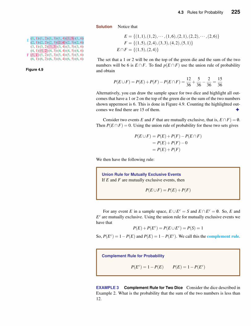
4.3 Rules for Probability 225
Solution Notice that
E = {(1,1),(1,2), · · · ,(1,6),(2,1),(2,2), · · · ,(2,6)}F = {(1,5),(2,4),(3,3),(4,2),(5,1)}
E ∩F = {(1,5),(2,4)}
The set that a 1 or 2 will be on the top of the green die and the sum of the two
Figure 4.9numbers will be 6 is E ∩F . To find p(E ∩F) use the union rule of probability
and obtain
P(E ∪F) = P(E)+P(F)−P(E ∩F) =12
36+
5
36− 2
36=
15
36
Alternatively, you can draw the sample space for two dice and highlight all out-
comes that have a 1 or 2 on the top of the green die or the sum of the two numbers
shown uppermost is 6. This is done in Figure 4.9. Counting the highlighted out-
comes we find there are 15 of them. ✦
Consider two events E and F that are mutually exclusive, that is, E ∩F) = /0.
Then P(E ∩F) = 0. Using the union rule of probability for these two sets gives
P(E ∪F) = P(E)+P(F)−P(E ∩F)
= P(E)+P(F)−0
= P(E)+P(F)
We then have the following rule:
Union Rule for Mutually Exclusive Events
If E and F are mutually exclusive events, then
P(E ∪F) = P(E)+P(F)
For any event E in a sample space, E ∪Ec = S and E ∩Ec = /0. So, E and
Ec are mutually exclusive. Using the union rule for mutually exclusive events we
have that
P(E)+P(Ec) = P(E ∪Ec) = P(S) = 1
So, P(Ec) = 1−P(E) and P(E) = 1−P(Ec). We call this the complement rule.
Complement Rule for Probability
P(Ec) = 1−P(E) P(E) = 1−P(Ec)
EXAMPLE 3 Complement Rule for Two Dice Consider the dice described in
Example 2. What is the probability that the sum of the two numbers is less than
12.
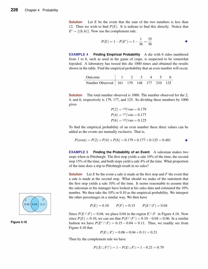
226 Chapter 4 Probability
Solution Let E be the event that the sum of the two numbers is less than
12. Then we wish to find P(E). It is tedious to find this directly. Notice that
Ec = {(6,6)}. Now use the complement rule.
P(E) = 1−P(Ec) = 1− 1
36=
35
36✦
EXAMPLE 4 Finding Empirical Probability A die with 6 sides numbered
from 1 to 6, such as used in the game of craps, is suspected to be somewhat
lopsided. A laboratory has tossed this die 1000 times and obtained the results
shown in the table. Find the empirical probability that an even number will occur.
Outcome 1 2 3 4 5 6
Number Observed 161 179 148 177 210 125
Solution The total number observed is 1000. The number observed for the 2,
4, and 6, respectively is 179, 177, and 125. So dividing these numbers by 1000
gives
P(2) = 179/1000 = 0.179
P(4) = 177/1000 = 0.177
P(6) = 125/1000 = 0.125
To find the empirical probability of an even number these three values can be
added as the events are mutually exclusive. That is,
P(even) = P(2)+P(4)+P(6) = 0.179+0.177+0.125 = 0.481 ✦
EXAMPLE 5 Finding the Probability of an Event A salesman makes two
stops when in Pittsburgh. The first stop yields a sale 10% of the time, the second
stop 15% of the time, and both stops yield a sale 4% of the time. What proportion
of the time does a trip to Pittsburgh result in no sales?
Solution Let E be the event a sale is made at the first stop and F the event that
a sale is made at the second stop. What should we make of the statement that
the first stop yields a sale 10% of the time. It seems reasonable to assume that
the salesman or his manager have looked at his sales data and estimated the 10%
number. We then take the 10% or 0.10 as the empirical probability. We interpret
the other percentages in a similar way. We then have
P(E) = 0.10 P(F) = 0.15 P(E ∩F) = 0.04
Since P(E ∩F) = 0.04, we place 0.04 in the region E ∩F in Figure 4.10. Now
Figure 4.10since P(E) = 0.10, we can see that P(E ∩Fc) = 0.10−0.04 = 0.06. In a similar
fashion we have P(Ec ∩F) = 0.15− 0.04 = 0.11. Thus, we readily see from
Figure 4.10 that
P(E ∪F) = 0.06+0.04+0.11 = 0.21
Then by the complement rule we have
P((E ∪F)c) = 1−P(E ∪F) = 1−0.21 = 0.79
4.3 Rules for Probability 227
Thus no sale is made in Pittsburgh 79% of the time. ✦
REMARK: We could have obtained P(E ∪F) directly from the union rule as
follows:
P(E ∪F) = P(E)+P(F)−P(E ∩F) = 0.10+0.15−0.04 = 0.21
EXAMPLE 6 Finding the Probability of an Event The probability that any
of the first five numbers of a loaded die will come up is the same while the
probability that a 6 comes up is 0.25. What is the probability that a 1 will come
up?
Solution We are given P(1) = P(2) = P(3) = P(4) = P(5), P(6) = 0.25. Also,
all the probabilities must add up to 1, so
1 = P(1)+P(2)+P(3)+P(4)+P(5)+P(6)
= 5P(1)+0.25
5P(1) = 0.75
P(1) = 0.15 ✦
EXAMPLE 7 Continuous Sample Space Arrange the following information
in a probability distribution table: A crop of apples is brought in for weighing. It
is found that 10% of the apples weigh less than 100 gm, 40% weigh 200 gm or
less, and 25% weigh more than 300 gm.
Solution If we let x = weight of an apple in grams then
Event Probability
0 ≤ x < 100 gm 0.10
100 gm ≤ x≤ 200 gm 0.30
200 gm < x≤ 300 gm 0.35
x > 300 gm 0.25
Note that the 40% of the apples that weigh 200 gm or less includes the 10%
that weigh less than 100 grams. Since the events in a probability distribution
table must be mutually exclusive, the 30% that weigh 100 grams or more and
200 grams or less are shown in the second row. The third row of the table is
found using deductive reasoning as the total probability must be 1 and there is a
gap in the events. ✦
✧ Odds (Optional)
One can interpret probabilities in terms of odds in a bet. Suppose in a sample
space S we are given an event E with probability P = P(E) = 5/7. In the long
term we expect E to occur 5 out of 7 times. Now, P(Ec) = 2/7 and in the long
term we expect that Ec to occur 2 out of 7 times. Then we say that the odds in
favor of E are 5 to 2 or 5:2.
228 Chapter 4 Probability
Odds
The odds in favor of an event E are defined to be the ratio of P(E) to
P(Ec),P(E) : P(Ec) or P(E) : (1−P(E))
Often the ratio P(E):P(Ec) is reduced to lowest terms, a:b, and then we say
that the odds are a to b.
EXAMPLE 8 Determining the Odds of an Event You believe that a horse has
a probability of 1/4 of winning a race. What are the odds of this horse winning?
What are the odds of this horse losing? What profit should a winning $2 bet
return to be fair?
Solution Since the probability of winning is P = 1/4, the odds of winning are
P : (1−P) → 1
4:
(
1− 1
4
)
→ 1
4:
3
4→ 1 : 3 or 1 to 3
With the probability of winning at 1/4, the probability of losing is 1− 1/4 = 3/4.
Then the odds for losing are
3
4:
(
1− 3
4
)
→ 3
4:
1
4→ 3 : 1
Since the ratio 3 : 1 can also be written as 6:2 with odds 6 to 2, a fair $2 bet should
return $6 for a winning ticket. ✦
Notice that making this same bet many times, we expect to win $6 one-fourth
of the time and lose $2 three-fourths of the time. So, for example, on every
four bets we would expect to win $6 once and lose $2 three times. Our average
winnings would be 6(1)−2(3) = 0 dollars.
If the odds for an event E are given as a : b, we can calculate the probability
P(E). We have
a
b=
P(E)
1−P(E)
a(1−P(E)) = bP(E)
a = bP(E)+aP(E)
= P(E)(a+b)
P(E) =a
a+b
Obtaining Probability From Odds
Suppose that the odds for an event E occurring is given as a to b or a : b,
then
P(E) =a
a+b
4.3 Rules for Probability 229
REMARK: One can think of the odds a : b of event E as saying if this experiment
was carried out a+ b times, then a of those times E would have occurred. Our
definition of empirical probability then says P(E) = a/a+b
EXAMPLE 9 Obtaining Probability From Odds At the race track, the odds
for a horse winning is listed at 3 : 2. What is the probability that the horse will
win.
Solution Using the above formula for odds a : b, we have
P =a
a+b=
3
3+2= 0.60 ✦
Self-Help Exercises 4.3
1. If S= {a,b,c}with P(a) =P(b) = 2P(c), find P(a).
2. A company has bids on two contracts. They believe
that the probability of obtaining the first contract
is 0.4 and of obtaining the second contract is 0.3,
while the probability of obtaining both contracts is
0.1.
a. Find the probability that they will obtain exactly
one of the contracts.
b. Find the probability that they will obtain neither
of the contracts.
3. What are the odds that the company in the previous
exercise will obtain both of the contracts?
4.3 Exercises
In all the following, S is assumed to be a sample space.
1. Let S = {a,b,c} with P(a) = 0.1, P(b) = 0.4, and
P(c) = 0.5. Let E = {a,b} and F = {b,c}. Find
P(E) and P(F).
2. Let S= {a,b,c,d,e, f}with P(a) = 0.1, P(b) = 0.2,
P(c) = 0.25, P(d) = 0.15, P(e) = 0.12, and P( f ) =0.18. Let E = {a,b,c} and F = {c,d,e, f} and find
P(E) and P(F).
3. Let S = {a,b,c,d,e, f} with P(b) = 0.2, P(c) =0.25, P(d) = 0.15, P(e) = 0.12, and P( f ) = 0.1.
Let E = {a,b,c} and F = {c,d,e, f}. Find P(a),P(E), and P(F).
4. Let S = {a,b,c,d,e, f} with P(b) = 0.3, P(c) =0.15 , P(d) = 0.05, P(e) = 0.2, P( f ) = 0.13. Let
E = {a,b,c} and F = {c,d,e, f}. Find P(a), P(E),and P(F).
5. If S = {a,b,c,d} with P(a) = P(b) = P(c) = P(d),find P(a).
6. If S = {a,b,c} with P(a) = P(b) and P(c) = 0.4,
find P(a).
7. If S = {a,b,c,d,e, f} with P(a) = P(b) = P(c) =P(d) = P(e) = P( f ), find P(a).
8. If S = {a,b,c} with P(a) = 2P(b) = 3P(c), find
P(a).
9. If S = {a,b,c,d,e, f} with P(a) = P(b) = P(c) and
P(d) = P(e) = P( f ) = 0.1, find P(a).
10. If S = {a,b,c,d,e, f} with P(a) = P(b) = P(c),P(d) = P(e) = P( f ), and P(d) = 2P(a), find P(a).
11. If E and F are two disjoint events in S with P(E) =0.2 and P(F) = 0.4, find P(E ∪ F), P(Ec), and
P(E ∩F).
12. Why is it not possible for E and F to be two disjoint
events in S with P(E) = 0.5 and P(F) = 0.7?
13. If E and F are two disjoint events in S with P(E) =0.4 and P(F)= 0.3, find P(E∪F), P(Fc), P(E∩F),P((E ∪F)c), and P((E ∩F)c).
14. Why is it not possible for S = {a,b,c} with P(a) =0.3, P(b) = 0.4, and P(c) = 0.5?
230 Chapter 4 Probability
15. Let E and F be two events in S with P(E) = 0.3,
P(F) = 0.5, and P(E ∩ F) = 0.2. Find P(E ∪ F)and P(E ∩Fc).
16. Let E and F be two events in S with P(E) = 0.3,
P(F) = 0.5, and P(E ∩F) = 0.2. Find P(Ec ∩F)and P(Ec∩Fc).
17. Let E and F be two events in S with P(E) = 0.3,
P(F) = 0.5, and P(E ∪ F) = 0.6. Find P(E ∩ F)and P(E ∩Fc).
18. Why is it not possible to have E and F two events
in S with P(E) = 0.3 and P(E ∩F) = 0.5?
In Exercises 19 through 22, let E, F , and G be events
in S with P(E) = 0.55, P(F) = 0.4, P(G) = 0.45,
P(E ∩F) = 0.3, P(E ∩G) = 0.2, P(F ∩G) = 0.15, and
P(E ∩F ∩G) = 0.1.
19. Find P(E ∩F ∩Gc), P(E ∩Fc∩G), and P(E ∩Fc∩Gc).
20. Using the results of the previous exercise, find
P(Ec∩F ∩G), P(Ec∩F ∩Gc), and P(Ec∩Fc∩G).
21. Using the results of the previous two exercises, find
P(E ∪F ∪G).
22. Using the results of the previous three exercises,
find P(Ec∪Fc∪Gc).
23. For the loaded die in Example 6 zzz of the text, what
are the odds that
a. a 2 will occur b. a 6 will occur?
24. For the loaded die in Example 6 zzz of the text, what
are the odds that
a. a 3 will occur b. a 1 will occur?
25. A company believes it has a probability of 0.40 of
receiving a contract. What is the odds that it will?
26. In Example 5 zzz of the text, what are the odds that
the salesman will make a sale on
a. the first stop b. on the second stop
c. on both stops?
27. It is known that the odds that E will occur are 1:3
and that the odds that F will occur are 1:2, and that
both E and F cannot occur. What are the odds that
E or F will occur?
28. If the odds for a successful marriage are 1:2, what
is the probability for a successful marriage?
29. If the odds for the Giants winning the World Series
are 1:4, what is the probability that the Giants will
win the Series?
Applications
30. Bidding on Contracts An aerospace firm has three
bids on government contracts and knows that the
contracts are most likely to be divided up among
a number of companies. The firm decides that the
probability of obtaining exactly one contract is 0.6,
of exactly two contracts is 0.15, and of exactly three
contracts is 0.04. What is the probability that the
firm will obtain at least one contracts? No con-
tracts?
31. Quality Control An inspection of computers manu-
factured at a plant reveals that 2% of the monitors
are defective, 3% of the keyboards are defective,
and 1% of the computers have both defects.
a. Find the probability that a computer at this plant
has at least one of these defects.
b. Find the probability that a computer at this plant
has none of these defects.
32. Medicine A new medication produces headaches in
5% of the users, upset stomach in 15%, and both in
2%.
a. Find the probability that at least one of these side
effects occurs.
b. Find the probability that neither of these side ef-
fects occurs.
33. Manufacturing A manufactured item is guaranteed
for one year and has three critical parts. It has been
decided that during the first year the probability of
failure of the first part is 0.03, of the second part
0.02, the third part 0.01, both the first and second is
0.005, both the first and third is 0.004, both the sec-
ond and third is 0.003, and all three parts 0.001.
a. What is the probability that exactly one of these
parts will fail in the first year?
b. What is the probability that at least one of these
parts will fail in the first year?
c. What is the probability that none of these parts
will fail in the first year?
34. Marketing A survey of business executives found
that 40% read Business Week, 50% read Fortune,
40% read Money, 17% read both Business Week and
Fortune, 15% read both both Business Week and
Money, 14% read both Fortune and Money, and 8%
read all three of these magazines.
4.3 Rules for Probability 231
a. What is the probability that one of these execu-
tives reads exactly one of these three magazines?
b. What is the probability that one of these execu-
tives reads at least one of these three magazines?
c. What is the probability that one of these execu-
tives reads none of these three magazines?
35. Advertising A firm advertises three different prod-
ucts, A, B, and C, on television. From past expe-
rience, it expects 1.5% of listeners to buy exactly
one of the products, 1% to buy exactly two of the
products, 1.2% to buy A, 0.4% to buy both A and
B, 0.3% to buy both A and C, and 0.6% to buy A
but not the other two.
a. Find the probability that a listener will buy only
B or only C.
b. Find the probability that a listener will buy all
three.
c. Find the probability that a listener will buy both
B and C.
d. Find the probability that a listener will buy none
of the three.
36. Sales A salesman always makes a sale at one of the
three stops in Atlanta and 30% of the time makes
a sale at only the first stop, 15% at only the sec-
ond stop, 20% at only the third stop, and 35% of the
time at exactly two of the stops. Find the probability
that the salesman makes a sale at all three stops in
Atlanta.
Extensions
37. Let E and F be two events in S with P(E) = 0.5 and
P(F) = 0.7. Just how small could P(E∩F) possibly
be?
38. Let E and F be two events in S with P(E) = 0.3 and
P(F) = 0.4. Just how large could P(F∪F) possibly
be?
39. You buy a new die and toss it 1000 times. A 1 comes
up 165 times. Is it true that the probability of a 1
showing on this die is 0.165?
40. A fair coin is to be tossed 100 times. Naturally you
expect tails to come up 50 times. After 60 tosses,
heads has come up 40 times. Is it true that now
heads is likely to come up less often than tails dur-
ing the next 40 tosses?
41. You are playing a game at a casino and have cor-
rectly calculated the probability of winning any one
game to be 0.48. You have played for some time
and have won 60% of the time. You are on a roll.
Should you keep playing?
42. You are watching a roulette game at a casino and
notice that red has been coming up unusually of-
ten. (Red should come up as often as black.) Is it
true that, according to “the law of averages,” black
is likely to come up unusually often in the next num-
ber of games to “even things up”?
43. You buy a die and toss it 1000 times and notice that
a 1 came up 165 times. You decide that the probabil-
ity of a 1 on this die is 0.165. Your friend takes this
die and tosses it 1000 times and notes that a 1 came
up 170 times. He concludes that the probability of a
1 is 0.17. Who is correct?
44. People who frequent casinos and play lotteries are
gamblers, but those who run the casinos and lotter-
ies are not. Do you agree? Why or why not?
Solutions to Self-Help Exercises 4.3
1. If S = {a,b,c} and P(a) = P(b) = 2P(c), then
1 = P(a)+P(b)+P(c)
= P(a)+P(a)+0.5P(a)
= 2.5P(a)
P(a) = 0.4
2.
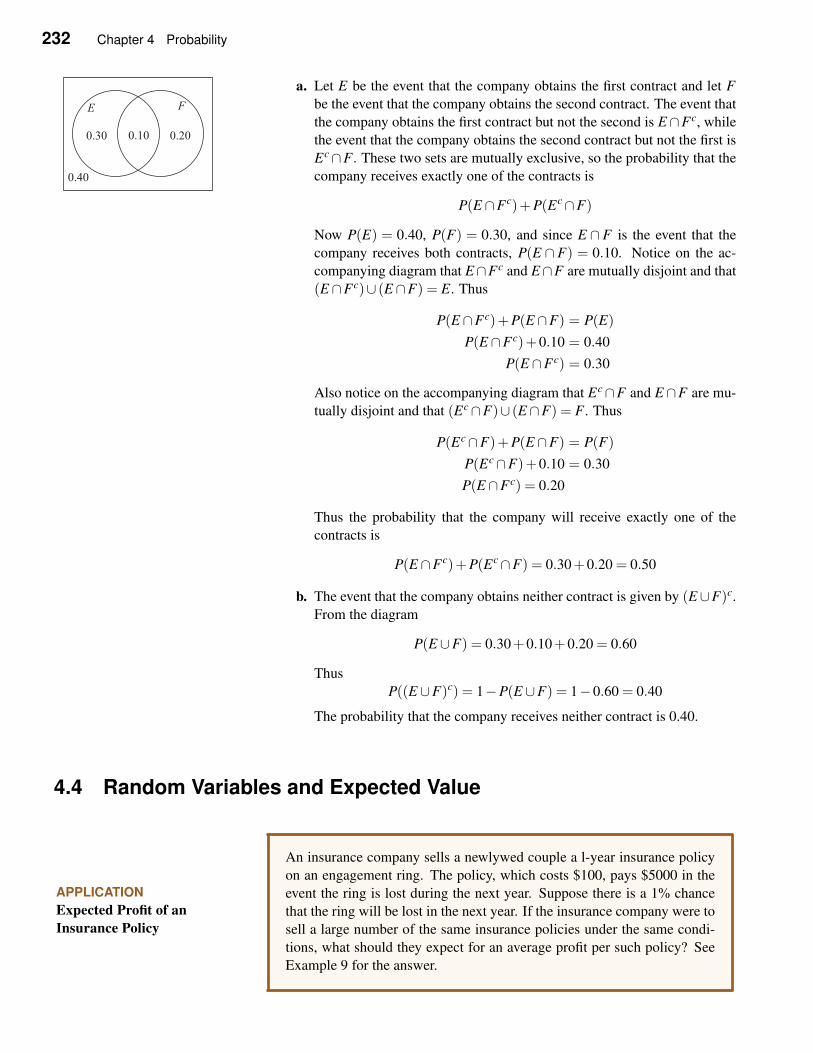
232 Chapter 4 Probability
a. Let E be the event that the company obtains the first contract and let F
be the event that the company obtains the second contract. The event that
the company obtains the first contract but not the second is E ∩Fc, while
the event that the company obtains the second contract but not the first is
Ec∩F . These two sets are mutually exclusive, so the probability that the
company receives exactly one of the contracts is
P(E ∩Fc)+P(Ec∩F)
Now P(E) = 0.40, P(F) = 0.30, and since E ∩F is the event that the
company receives both contracts, P(E ∩F) = 0.10. Notice on the ac-
companying diagram that E∩Fc and E∩F are mutually disjoint and that
(E ∩Fc)∪ (E ∩F) = E. Thus
P(E ∩Fc)+P(E ∩F) = P(E)
P(E ∩Fc)+0.10 = 0.40
P(E ∩Fc) = 0.30
Also notice on the accompanying diagram that Ec∩F and E ∩F are mu-
tually disjoint and that (Ec∩F)∪ (E ∩F) = F . Thus
P(Ec∩F)+P(E ∩F) = P(F)
P(Ec∩F)+0.10 = 0.30
P(E ∩Fc) = 0.20
Thus the probability that the company will receive exactly one of the
contracts is
P(E ∩Fc)+P(Ec∩F) = 0.30+0.20 = 0.50
b. The event that the company obtains neither contract is given by (E∪F)c.
From the diagram
P(E ∪F) = 0.30+0.10+0.20 = 0.60
Thus
P((E ∪F)c) = 1−P(E ∪F) = 1−0.60 = 0.40
The probability that the company receives neither contract is 0.40.
4.4 Random Variables and Expected Value
APPLICATION
Expected Profit of an
Insurance Policy
An insurance company sells a newlywed couple a l-year insurance policy
on an engagement ring. The policy, which costs $100, pays $5000 in the
event the ring is lost during the next year. Suppose there is a 1% chance
that the ring will be lost in the next year. If the insurance company were to
sell a large number of the same insurance policies under the same condi-
tions, what should they expect for an average profit per such policy? See
Example 9 for the answer.
4.4 Random Variables and Expected Value 233
In this section we wish to see how to present numerical data in a manner that will
permit making interpretations and comparisons. First, we define the important
idea of a “random variable.”
✧ Random Variables
The outcomes of many experiments are numbers. For example, the number
shown uppermost on a six-sided dice that has been tossed is {1,2,3,4,5,6}. But
outcomes of experiments are not always real numbers. The outcomes of experi-
ments can be “an even number,” “heads,” “above average,” or “defective,” none
of which are real numbers. However, it is often useful to assign a real number
to each outcome of an experiment. For example, the outcome of the experiment
“your grade in math” is a letter. But for purposes that you are well aware of, each
letter is assigned a real number. Typically 4 is assigned to an A, 3 to a B, 2 to a
C, 1 to a D, and 0 to an F.
Usually there is some rational basis on which the assignment of a real number
to an outcome is made. For example, since a grade of A is “better” than a grade
of B, it makes sense to assign a higher number to the grade A than to B. Also
the assignment of the numbers to each letter is done in such a manner that the
numerical difference between two successive letters will be equal. Assigning
zero to F makes sense since no credit is given for a grade of F. Finally, using the
numbers 0, 1, 2, 3, and 4 makes it easy to calculate the “average” grade and for
this number to have a readily understood meaning.
When numbers are assigned to the outcomes of experiments according to
some rule or function, we refer to the function as a random variable. As we
have seen in assigning numbers to letter grades, the assignments of numbers to
the outcomes of experiments are normally done in a manner that is reasonable
and, most importantly, in a manner that permits these numbers to be used for
interpretation and comparison.
Random Variables
A random variable is a rule that assigns precisely one real number to each
outcome of an experiment.
REMARK: Unless otherwise specified, when the outcomes of an experiment
are themselves numbers, the random variable is the rule that simply assigns each
number to itself.
EXAMPLE 1 Random Variables A fair coin is flipped three times. We want
to determine the probability of the events “3 heads have appeared,” “exactly 2
heads have appeared,” and so on. Associate a random variable with the outcomes
and determine a probability distribution for the random variable.
Solution First list all the eight possible sequences of heads (H) and tails (T ).
{(HHH),(HHT ),(HTH),(HTT ),(TT T ),(TT H),(THT ),(THH)}
From this list we note how many times heads appear.
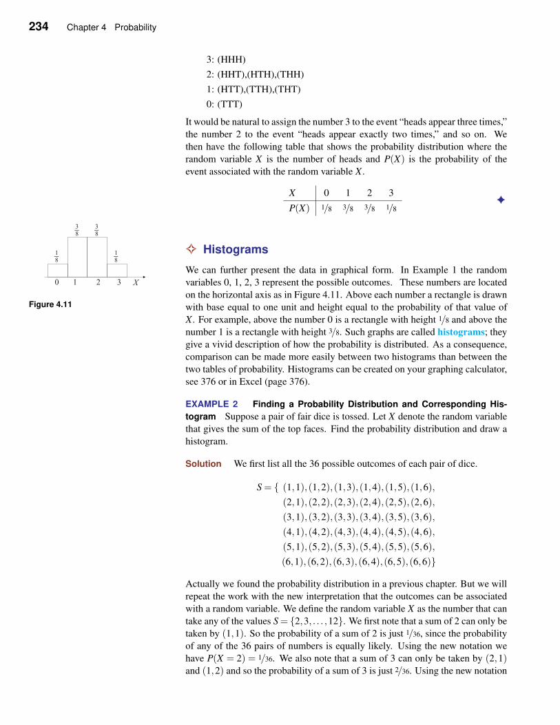
234 Chapter 4 Probability
3: (HHH)
2: (HHT),(HTH),(THH)
1: (HTT),(TTH),(THT)
0: (TTT)
It would be natural to assign the number 3 to the event “heads appear three times,”
the number 2 to the event “heads appear exactly two times,” and so on. We
then have the following table that shows the probability distribution where the
random variable X is the number of heads and P(X) is the probability of the
event associated with the random variable X .
X 0 1 2 3
P(X) 1/8 3/8 3/8 1/8✦
✧ Histograms
We can further present the data in graphical form. In Example 1 the random
variables 0, 1, 2, 3 represent the possible outcomes. These numbers are located
Figure 4.11on the horizontal axis as in Figure 4.11. Above each number a rectangle is drawn
with base equal to one unit and height equal to the probability of that value of
X . For example, above the number 0 is a rectangle with height 1/8 and above the
number 1 is a rectangle with height 3/8. Such graphs are called histograms; they
give a vivid description of how the probability is distributed. As a consequence,
comparison can be made more easily between two histograms than between the
two tables of probability. Histograms can be created on your graphing calculator,
see 376 or in Excel (page 376).
EXAMPLE 2 Finding a Probability Distribution and Corresponding His-
togram Suppose a pair of fair dice is tossed. Let X denote the random variable
that gives the sum of the top faces. Find the probability distribution and draw a
histogram.
Solution We first list all the 36 possible outcomes of each pair of dice.
S = { (1,1),(1,2),(1,3),(1,4),(1,5),(1,6),
(2,1),(2,2),(2,3),(2,4),(2,5),(2,6),
(3,1),(3,2),(3,3),(3,4),(3,5),(3,6),
(4,1),(4,2),(4,3),(4,4),(4,5),(4,6),
(5,1),(5,2),(5,3),(5,4),(5,5),(5,6),
(6,1),(6,2),(6,3),(6,4),(6,5),(6,6)}
Actually we found the probability distribution in a previous chapter. But we will
repeat the work with the new interpretation that the outcomes can be associated
with a random variable. We define the random variable X as the number that can
take any of the values S = {2,3, . . . ,12}. We first note that a sum of 2 can only be
taken by (1,1). So the probability of a sum of 2 is just 1/36, since the probability
of any of the 36 pairs of numbers is equally likely. Using the new notation we
have P(X = 2) = 1/36. We also note that a sum of 3 can only be taken by (2,1)and (1,2) and so the probability of a sum of 3 is just 2/36. Using the new notation
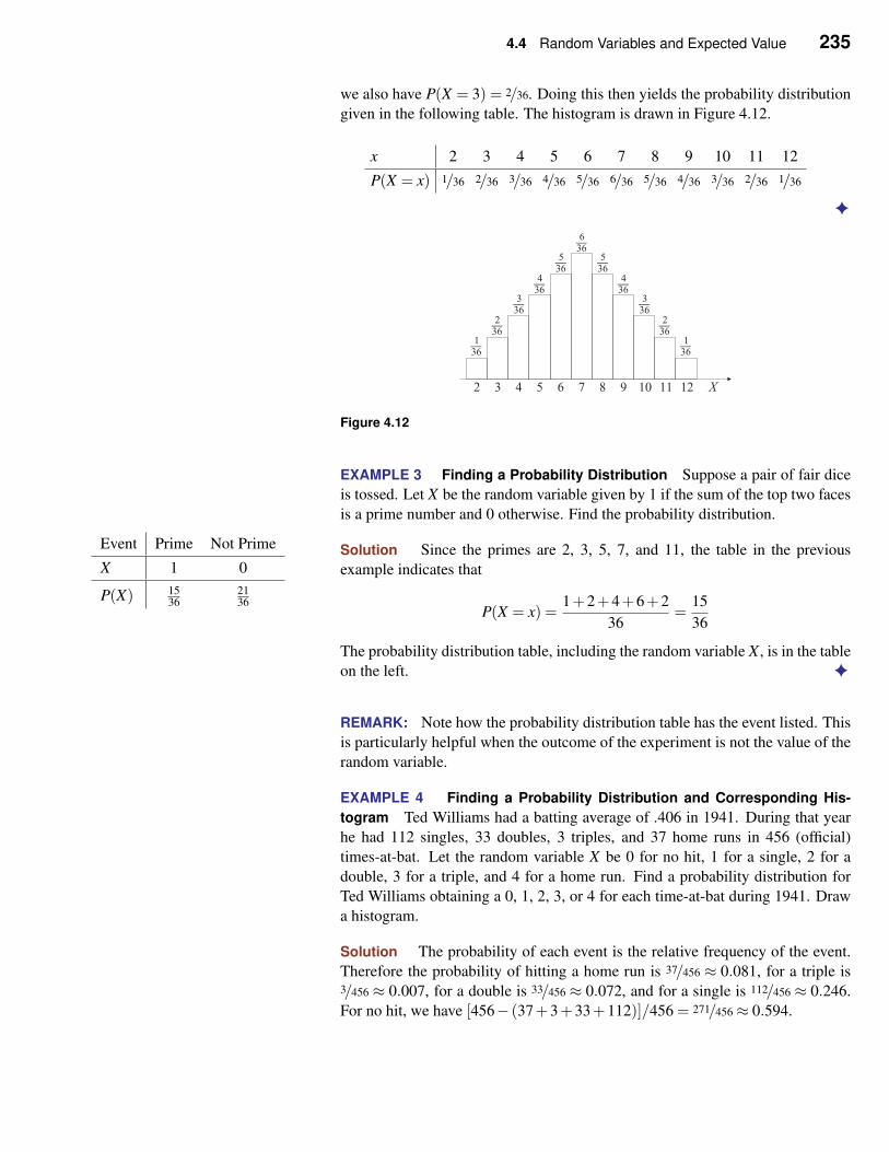
4.4 Random Variables and Expected Value 235
we also have P(X = 3) = 2/36. Doing this then yields the probability distribution
given in the following table. The histogram is drawn in Figure 4.12.
x 2 3 4 5 6 7 8 9 10 11 12
P(X = x) 1/36 2/36 3/36 4/36 5/36 6/36 5/36 4/36 3/36 2/36 1/36
✦
Figure 4.12
EXAMPLE 3 Finding a Probability Distribution Suppose a pair of fair dice
is tossed. Let X be the random variable given by 1 if the sum of the top two faces
is a prime number and 0 otherwise. Find the probability distribution.
Solution Since the primes are 2, 3, 5, 7, and 11, the table in the previous
example indicates that
Event Prime Not Prime
X 1 0
P(X) 1536
2136
P(X = x) =1+2+4+6+2
36=
15
36
The probability distribution table, including the random variable X , is in the table
on the left. ✦
REMARK: Note how the probability distribution table has the event listed. This
is particularly helpful when the outcome of the experiment is not the value of the
random variable.
EXAMPLE 4 Finding a Probability Distribution and Corresponding His-
togram Ted Williams had a batting average of .406 in 1941. During that year
he had 112 singles, 33 doubles, 3 triples, and 37 home runs in 456 (official)
times-at-bat. Let the random variable X be 0 for no hit, 1 for a single, 2 for a
double, 3 for a triple, and 4 for a home run. Find a probability distribution for
Ted Williams obtaining a 0, 1, 2, 3, or 4 for each time-at-bat during 1941. Draw
a histogram.
Solution The probability of each event is the relative frequency of the event.
Therefore the probability of hitting a home run is 37/456 ≈ 0.081, for a triple is3/456 ≈ 0.007, for a double is 33/456 ≈ 0.072, and for a single is 112/456 ≈ 0.246.
For no hit, we have [456− (37+3+33+112)]/456 = 271/456≈ 0.594.
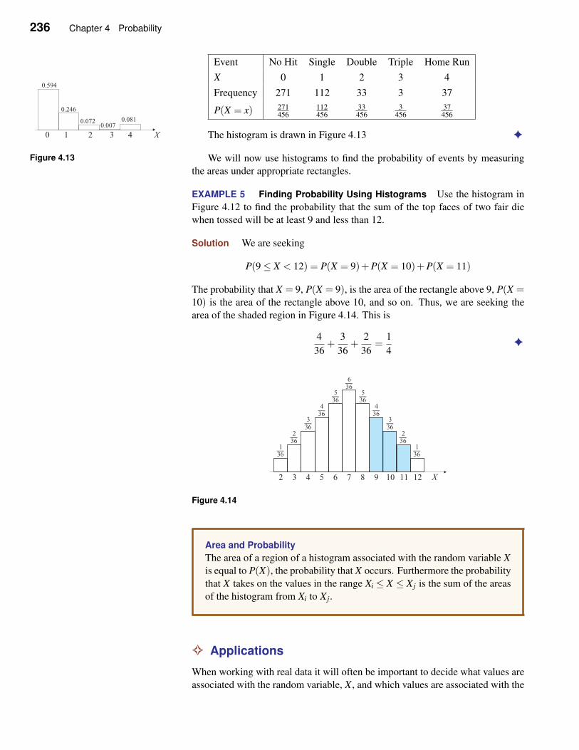
236 Chapter 4 Probability
Event No Hit Single Double Triple Home Run
X 0 1 2 3 4
Frequency 271 112 33 3 37
P(X = x) 271456
112456
33456
3456
37456
The histogram is drawn in Figure 4.13 ✦
Figure 4.13 We will now use histograms to find the probability of events by measuring
the areas under appropriate rectangles.
EXAMPLE 5 Finding Probability Using Histograms Use the histogram in
Figure 4.12 to find the probability that the sum of the top faces of two fair die
when tossed will be at least 9 and less than 12.
Solution We are seeking
P(9≤ X < 12) = P(X = 9)+P(X = 10)+P(X = 11)
The probability that X = 9, P(X = 9), is the area of the rectangle above 9, P(X =10) is the area of the rectangle above 10, and so on. Thus, we are seeking the
area of the shaded region in Figure 4.14. This is
4
36+
3
36+
2
36=
1
4✦
Figure 4.14
Area and Probability
The area of a region of a histogram associated with the random variable X
is equal to P(X), the probability that X occurs. Furthermore the probability
that X takes on the values in the range Xi ≤ X ≤ X j is the sum of the areas
of the histogram from Xi to X j.
✧ Applications
When working with real data it will often be important to decide what values are
associated with the random variable, X , and which values are associated with the
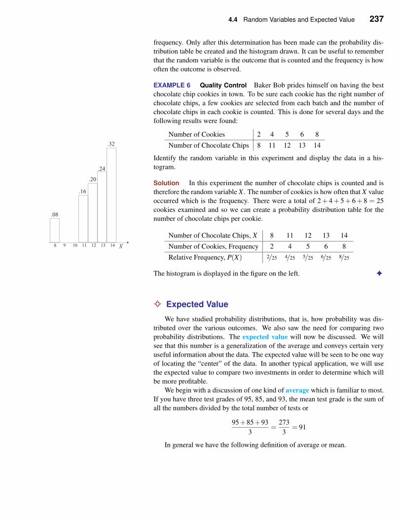
4.4 Random Variables and Expected Value 237
frequency. Only after this determination has been made can the probability dis-
tribution table be created and the histogram drawn. It can be useful to remember
that the random variable is the outcome that is counted and the frequency is how
often the outcome is observed.
EXAMPLE 6 Quality Control Baker Bob prides himself on having the best
chocolate chip cookies in town. To be sure each cookie has the right number of
chocolate chips, a few cookies are selected from each batch and the number of
chocolate chips in each cookie is counted. This is done for several days and the
following results were found:
Number of Cookies 2 4 5 6 8
Number of Chocolate Chips 8 11 12 13 14
Identify the random variable in this experiment and display the data in a his-
togram.
Solution In this experiment the number of chocolate chips is counted and is
therefore the random variable X . The number of cookies is how often that X value
occurred which is the frequency. There were a total of 2+ 4+ 5+ 6+ 8 = 25
cookies examined and so we can create a probability distribution table for the
number of chocolate chips per cookie.
Number of Chocolate Chips, X 8 11 12 13 14
Number of Cookies, Frequency 2 4 5 6 8
Relative Frequency, P(X) 2/25 4/25 5/25 6/25 8/25
The histogram is displayed in the figure on the left. ✦
✧ Expected Value
We have studied probability distributions, that is, how probability was dis-
tributed over the various outcomes. We also saw the need for comparing two
probability distributions. The expected value will now be discussed. We will
see that this number is a generalization of the average and conveys certain very
useful information about the data. The expected value will be seen to be one way
of locating the “center” of the data. In another typical application, we will use
the expected value to compare two investments in order to determine which will
be more profitable.
We begin with a discussion of one kind of average which is familiar to most.
If you have three test grades of 95, 85, and 93, the mean test grade is the sum of
all the numbers divided by the total number of tests or
95+85+93
3=
273
3= 91
In general we have the following definition of average or mean.
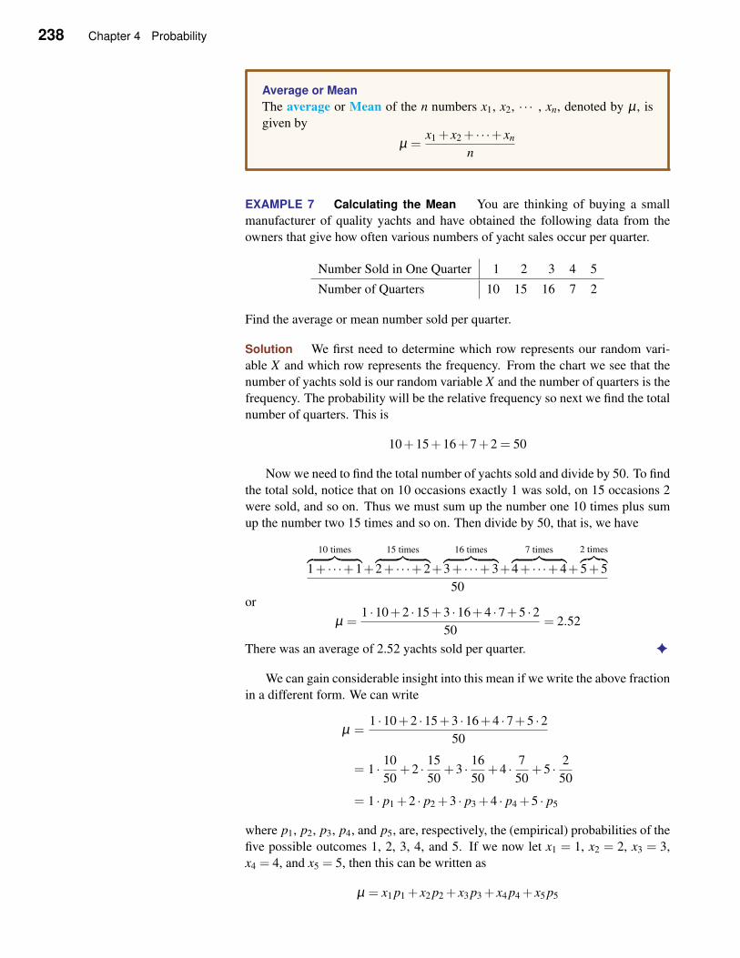
238 Chapter 4 Probability
Average or Mean
The average or Mean of the n numbers x1, x2, · · · , xn, denoted by µ , is
given by
µ =x1 + x2 + · · ·+ xn
n
EXAMPLE 7 Calculating the Mean You are thinking of buying a small
manufacturer of quality yachts and have obtained the following data from the
owners that give how often various numbers of yacht sales occur per quarter.
Number Sold in One Quarter 1 2 3 4 5
Number of Quarters 10 15 16 7 2
Find the average or mean number sold per quarter.
Solution We first need to determine which row represents our random vari-
able X and which row represents the frequency. From the chart we see that the
number of yachts sold is our random variable X and the number of quarters is the
frequency. The probability will be the relative frequency so next we find the total
number of quarters. This is
10+15+16+7+2 = 50
Now we need to find the total number of yachts sold and divide by 50. To find
the total sold, notice that on 10 occasions exactly 1 was sold, on 15 occasions 2
were sold, and so on. Thus we must sum up the number one 10 times plus sum
up the number two 15 times and so on. Then divide by 50, that is, we have
10 times︷ ︸︸ ︷
1+ · · ·+1+
15 times︷ ︸︸ ︷
2+ · · ·+2+
16 times︷ ︸︸ ︷
3+ · · ·+3+
7 times︷ ︸︸ ︷
4+ · · ·+4+
2 times︷︸︸︷
5+5
50or
µ =1 ·10+2 ·15+3 ·16+4 ·7+5 ·2
50= 2.52
There was an average of 2.52 yachts sold per quarter. ✦
We can gain considerable insight into this mean if we write the above fraction
in a different form. We can write
µ =1 ·10+2 ·15+3 ·16+4 ·7+5 ·2
50
= 1 · 10
50+2 · 15
50+3 · 16
50+4 · 7
50+5 · 2
50
= 1 · p1 +2 · p2 +3 · p3 +4 · p4 +5 · p5
where p1, p2, p3, p4, and p5, are, respectively, the (empirical) probabilities of the
five possible outcomes 1, 2, 3, 4, and 5. If we now let x1 = 1, x2 = 2, x3 = 3,
x4 = 4, and x5 = 5, then this can be written as
µ = x1 p1 + x2 p2 + x3 p3 + x4 p4 + x5 p5
4.4 Random Variables and Expected Value 239
This is the form we are seeking. Notice that each term is the product of an
outcome with the probability of that outcome. We call it the expected value. In
general we have the following, using the language of random variables.
Expected Value or Mean
Let X denote the random variable that has values x1, x2, . . . , xn, and let the
associated probabilities be p1, p2, . . . , pn. The expected value or mean
of the random variable X , denoted by E(X), is
E(X) = x1 p1 + x2 p2 · · ·+ xn pn
E(X) is what we “expect” over the long term. But we must realize that E(X)need not be an actual outcome. In Example 7, the expected value of sales per
quarter was 2.52. We cannot sell 2.52 yachts. Nonetheless, it is extremely useful
to think as though we could. (Actually, if the yacht manufacturer were incorpo-
rated with 100 shares outstanding and you owned one of these shares, it would
make a great deal of sense to say you sold 2.52 yachts.)
In the case that all the n outcomes are equally likely, the probabilities are just1/n and then
E(X) = x11
n+ x2
1
n+ · · ·+ xn
1
n=
x1 + x2 + · · ·+ xn
n
which is the mean.
EXAMPLE 8 Calculating the Expected Value Redo Example 7 using the
formula for E(X).
Solution Recall that we found the empirical probabilities to be p1 = 10/50 =0.20, p2 = 15/50 = 0.30, p3 = 16/50 = 0.32, p4 = 7/50 = 0.14, and p5 = 10/50 =0.04. Then
E(X) = x1 p1 + x2 p2 · · ·+ xn pn
= (1)(0.20)+(2)(0.30)+(3)(0.32)+(4)(0.14)+(5)(0.04)
= 2.52
Which is, of course, the same result as Example 7. ✦
✧ Applications
EXAMPLE 9 Calculating the Expected Value An insurance company sells a
newlywed couple a 1-year replacement insurance policy on an engagement ring.
The policy, which costs $100, pays $5000 in the event that the ring is lost during
the next year. If there is a 1% chance that the ring will be lost in the next year,
find the probability distribution for this financial transaction for the insurance
company and find their expected return. What meaning does this expected value
have to the insurance company?
240 Chapter 4 Probability
Solution If the ring is not lost during the next year, $100 is made by the
insurance company. If the ring is lost the next year, $5000 − $100 = $4900
is lost by the company. The random variable and the associated probability is
described in the following table.
Event Not Lost Lost
X 100 −4900
P(X) 0.99 0.01
Thus
E(X) = 100(0.99)−−4900(0.01) = 50
which is $50. If the insurance company were to sell a large number of the same
insurance policies under the same conditions, they would expect a $50 return per
policy. ✦
Suppose in considering buying the yacht manufacturer in Example 7, you wish to
take into account a principal competitor who also manufactures yachts. Knowl-
edge of the competitor’s profits would be useful in determining how competi-
tive the two manufacturers are and would heavily influence whether you actually
make the purchase. It would be convenient to know the details of the competi-
tor’s operations, but this is privileged information you are not likely to obtain.
You then hire some analysts who have considerable knowledge of the yacht busi-
ness and ask them to prepare a table like the one in the previous example that you
can use as a comparison. Naturally they are unable to give you exact figures, but
they give you the data in the table below.
Number Sold in One Quarter 0 1 2 3 4 5
Probability of Occurrence 0.10 0.20 0.30 0.25 0.10 0.05
Notice that they have assessed from their collective knowledge a probability
that the various outcomes will occur.
EXAMPLE 10 Calculating the Expected Value Suppose in Example 7 you
are told that the average profit per yacht is $20,000 and for the competitor, is
$21,000. Can you decide which company will have the higher profits per quarter?
Solution For Example 7, the average quarterly sales are 2.52 and the average
profit per yacht is $20,000, thus the average quarterly profit is
(2.52)($20,000) = $50,400
Looking now at the competitor the “expected” quarterly sales is
E(X) = (0)(0.10)+(1)(0.20)+(2)(0.30)+(3)(0.25)+(4)(0.10)+(5)(0.05) = 2.2
Thus you expect the competitor to sell 2.2 yachts per quarter. Their quarterly
profit is then expected to be
(2.2)($21,000) = $46,200
The profits of the competitor are less, so you feel more comfortable about the
purchase. ✦
4.4 Random Variables and Expected Value 241
There are two common versions of roulette: American and European. In the
European version of roulette the numbers from 0 to 36 are located at 37 equally
spaced slots on the wheel. Half of the numbers from 1 to 36 are red and the other
half are black. The zero slot is green. You place a bet on one or more numbers.
The wheel spins, and a ball falls randomly into one of the 37 slots.
EXAMPLE 11 Expected Value of a Bet In this bet select any of the 37
numbers. Making a $1 bet results in winning back $36 if your number occurs
and, of course, you lose your $1 if your number does not occur. Find the expected
return.
Solution A tree diagram is shown in Figure 4.15. There is a probability of
Figure 4.15
1/37 of winning and of 36/37 of losing. Let the random variable X be $35 if you
win and −$1 if you lose. Then the expected return is
E(X) = (35)1
37− (1)
36
37=− 1
37≈−0.027
On this bet you expect to lose about $.03 per $1 bet or 2.7% in the long run. ✦
Self-Help Exercises 4.4
1. Use the histogram in Figure 4.13 to find the prob-
ability that Ted Williams obtained an extra-base hit
(double, triple, or home run) during 1941.
2. In European roulette you can bet on a color, say red.
If red occurs, you win back twice your bet. If black
occurs, you lose your stake. If 0 occurs, the wheel
is spun again until 0 does not occur. If red occurs,
then you win the original stake back. If black comes
up, you lose your original stake. Find the expected
return. See page 241 for a description of this game.
4.4 Exercises
1. The grade distribution in a certain math class is
given in the following table.
Event A B C D F
Random Variable, x 4 3 2 1 0
Frequency 6 10 19 11 4
P(X = x)
Fill in the last row. Draw a histogram.
2. In 1961 Roger Maris set the record for most home
runs in a season that lasted until recent years. Com-
plete the following table, where 0 is associated with
no hit, 1 with a single, and so on.
Random Variable, x 0 1 2 3 4
Frequency 431 78 16 4 61
P(X = x)
3. The student ratings of a particular mathematics pro-
fessor are given in the following table. Complete
the last line and draw a histogram.
Event 1 2 3 4 5 6 7 8 9 10
Frequency 5 2 3 0 4 10 10 11 3 2
P(X = x)
4. A pair of fair dice is tossed. Let X be the random
variable given by the product of numbers on the top
faces of the dice. Find the probability distribution.
Draw a histogram.
5. A pair of fair dice is tossed. Let X be the random
variable given by the absolute value of the differ-
ence of the numbers on the top faces of the dice.
Find the probability distribution.
242 Chapter 4 Probability
6. The probability distribution of the random variable
X is given in the following table. What must z be?
Random Variable, x 0 1 2 3 4
P(X = x) 0.1 z 0.2 0.25 0.15
7. The probability distribution of the random variable
X is given in the following table. What must z be?
Random Variable, x 0 1 2 3 4
P(X = x) 0.2 0.1 0.1 z 0.3
8. The probability distribution of the random variable
(r. v.) X is given in the following table.
r. v., x −2 −1 0 1 2 3
P(X = x) .20 .15 .05 .35 .15 .10
Find the following probabilities
a. P(X = 0) b. P(X ≤ 0) c. P(−1 < X ≤ 4)d. P(X ≥ 1)
9. The probability distribution of the random variable
(r. v.) X is given in the following table.
r. v. x 4 5 6 7 8 9
P(X = x) 0.15 0.26 0.14 0.22 0.18 0.05
Find the following probabilities
a. P(X = 4) b. P(X ≤ 2) c. P(5≤ X ≤ 6)d. P(X ≥ 8).
10. Let Y be the random variable given by X2 where X
is given in Exercise 9. Find the probability distribu-
tion of Y .
11. Let Y be the random variable given by X +2 where
X is given in Exercise 9. Find the probability distri-
bution of Y .
12. If the random variable X denotes the real valued out-
comes given in the following table with the given
frequency of occurrence of each of the outcomes,
fill in the last line of the table and find E(X).
Outcome −2 −1 0 1 2 10
Frequency 10 11 9 9 5 6
P(X)
13. Find the expected value of the random variable X
having the probability distribution given in the fol-
lowing table.
X −30 −10 0 5 10 20
P(X) 0.15 0.25 0.05 0.10 0.25 0.20
14. Find the expected value of the random variable X
having the probability distribution given in the fol-
lowing table.
X −4 −1 0 1 2 3
P(X) 0.10 0.10 0.40 0.10 0.10 0.20
15. Babe Ruth established the all-time highest “slug-
ging average” for a single season in 1920. With
the random variable X assigned as indicated in the
following table with the associated probability, find
E(X) rounded to 3 decimal places. This is the “slug-
ging average.” We designated no hit by 0, single by
1, double by 2, and so on.
X 0 1 2 3 4
P(X) .6245 .1594 .0786 .0197 .1179
16. A student takes a single course during summer
school and decides that the probability of obtain-
ing each grade is as shown in the following table.
Find the expected grade point average for this sum-
mer; that is, find the expected value of the random
variable X .
Outcome A B C D F
X 4 3 2 1 0
P(X) 0.6 0.2 0.1 0.05 0.05
17. The annual returns for an investment over the last
three years are 50%, 0%, −50%. Find the average
annual return. Find the actual return over the three-
year period.
18. A two-year investment breaks even at the end of two
years but yielded a 50% loss in the first year. Find
the average annual rate of return for this investment.
19. For an advertising promotion a company is giving
away $10,000. All you have to do to enter is submit
a letter with your address on the entry form. The
winning entry will then be randomly selected, your
chance of winning being the same as anyone else’s.
If 100,000 people enter this contest and your only
cost is a 29-cent stamp, what is your expected re-
turn (to the nearest cent)?
20. In the daily numbers game, a person picks any of
the 1000 numbers from 0 to 999. A $1 wager on one
number will return $600 if that number hits; other-
wise nothing is returned. If the probability of any
one number is the same as that of any other, find the
expected return of this wager.
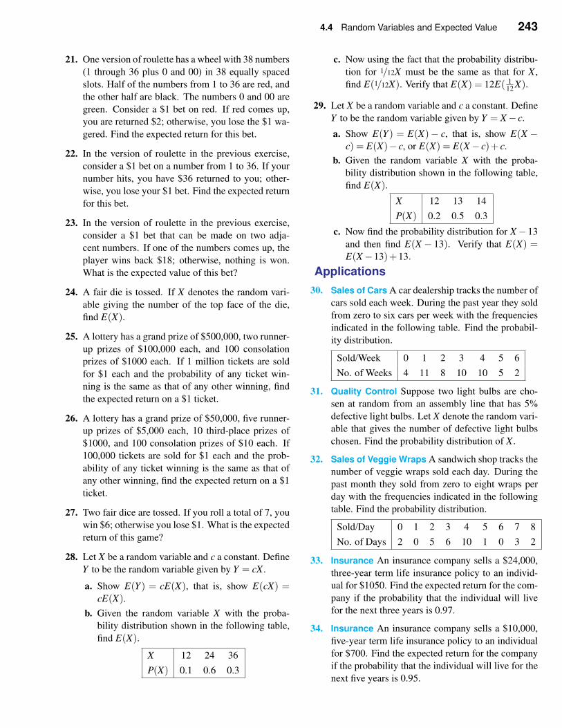
4.4 Random Variables and Expected Value 243
21. One version of roulette has a wheel with 38 numbers
(1 through 36 plus 0 and 00) in 38 equally spaced
slots. Half of the numbers from 1 to 36 are red, and
the other half are black. The numbers 0 and 00 are
green. Consider a $1 bet on red. If red comes up,
you are returned $2; otherwise, you lose the $1 wa-
gered. Find the expected return for this bet.
22. In the version of roulette in the previous exercise,
consider a $1 bet on a number from 1 to 36. If your
number hits, you have $36 returned to you; other-
wise, you lose your $1 bet. Find the expected return
for this bet.
23. In the version of roulette in the previous exercise,
consider a $1 bet that can be made on two adja-
cent numbers. If one of the numbers comes up, the
player wins back $18; otherwise, nothing is won.
What is the expected value of this bet?
24. A fair die is tossed. If X denotes the random vari-
able giving the number of the top face of the die,
find E(X).
25. A lottery has a grand prize of $500,000, two runner-
up prizes of $100,000 each, and 100 consolation
prizes of $1000 each. If 1 million tickets are sold
for $1 each and the probability of any ticket win-
ning is the same as that of any other winning, find
the expected return on a $1 ticket.
26. A lottery has a grand prize of $50,000, five runner-
up prizes of $5,000 each, 10 third-place prizes of
$1000, and 100 consolation prizes of $10 each. If
100,000 tickets are sold for $1 each and the prob-
ability of any ticket winning is the same as that of
any other winning, find the expected return on a $1
ticket.
27. Two fair dice are tossed. If you roll a total of 7, you
win $6; otherwise you lose $1. What is the expected
return of this game?
28. Let X be a random variable and c a constant. Define
Y to be the random variable given by Y = cX .
a. Show E(Y ) = cE(X), that is, show E(cX) =cE(X).
b. Given the random variable X with the proba-
bility distribution shown in the following table,
find E(X).
X 12 24 36
P(X) 0.1 0.6 0.3
c. Now using the fact that the probability distribu-
tion for 1/12X must be the same as that for X ,
find E(1/12X). Verify that E(X) = 12E( 112 X).
29. Let X be a random variable and c a constant. Define
Y to be the random variable given by Y = X− c.
a. Show E(Y ) = E(X)− c, that is, show E(X −c) = E(X)− c, or E(X) = E(X− c)+ c.
b. Given the random variable X with the proba-
bility distribution shown in the following table,
find E(X).
X 12 13 14
P(X) 0.2 0.5 0.3
c. Now find the probability distribution for X −13
and then find E(X − 13). Verify that E(X) =E(X−13)+13.
Applications
30. Sales of Cars A car dealership tracks the number of
cars sold each week. During the past year they sold
from zero to six cars per week with the frequencies
indicated in the following table. Find the probabil-
ity distribution.
Sold/Week 0 1 2 3 4 5 6
No. of Weeks 4 11 8 10 10 5 2
31. Quality Control Suppose two light bulbs are cho-
sen at random from an assembly line that has 5%
defective light bulbs. Let X denote the random vari-
able that gives the number of defective light bulbs
chosen. Find the probability distribution of X .
32. Sales of Veggie Wraps A sandwich shop tracks the
number of veggie wraps sold each day. During the
past month they sold from zero to eight wraps per
day with the frequencies indicated in the following
table. Find the probability distribution.
Sold/Day 0 1 2 3 4 5 6 7 8
No. of Days 2 0 5 6 10 1 0 3 2
33. Insurance An insurance company sells a $24,000,
three-year term life insurance policy to an individ-
ual for $1050. Find the expected return for the com-
pany if the probability that the individual will live
for the next three years is 0.97.
34. Insurance An insurance company sells a $10,000,
five-year term life insurance policy to an individual
for $700. Find the expected return for the company
if the probability that the individual will live for the
next five years is 0.95.
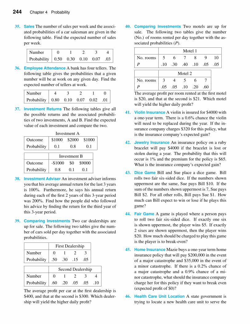
244 Chapter 4 Probability
35. Sales The number of sales per week and the associ-
ated probabilities of a car salesman are given in the
following table. Find the expected number of sales
per week.
Number 0 1 2 3 4
Probability 0.50 0.30 0.10 0.07 .03
36. Employee Attendance A bank has four tellers. The
following table gives the probabilities that a given
number will be at work on any given day. Find the
expected number of tellers at work.
Number 4 3 2 1 0
Probability 0.80 0.10 0.07 0.02 .01
37. Investment Returns The following tables give all
the possible returns and the associated probabili-
ties of two investments, A and B. Find the expected
value of each investment and compare the two.
Investment A
Outcome $1000 $2000 $1000
Probability 0.1 0.8 0.1
Investment B
Outcome -$1000 $0 $9000
Probability 0.8 0.1 0.1
38. Investment Adviser An investment adviser informs
you that his average annual return for the last 3 years
is 100%. Furthermore, he says his annual return
during each of the first 2 years of this 3-year period
was 200%. Find how the people did who followed
his advice by finding the return for the third year of
this 3-year period.
39. Comparing Investments Two car dealerships are
up for sale. The following two tables give the num-
ber of cars sold per day together with the associated
probabilities.
First Dealership
Number 0 1 2 3
Probability .50 .30 .15 .05
Second Dealership
Number 0 1 2 3 4
Probability .60 .20 .05 .05 .10
The average profit per car at the first dealership is
$400, and that at the second is $300. Which dealer-
ship will yield the higher daily profit?
40. Comparing Investments Two motels are up for
sale. The following two tables give the number
(No.) of rooms rented per day together with the as-
sociated probabilities (P).
Motel 1
No. rooms 5 6 7 8 9 10
P .10 .30 .40 .10 .05 .05
Motel 2
No. rooms 3 4 5 6 7
P .05 .05 .10 .20 .60
The average profit per room rented at the first motel
is $20, and that at the second is $21. Which motel
will yield the higher daily profit?
41. Violin Insurance A violin is insured for $4000 with
a one-year term. There is a 0.6% chance the violin
will need to be replaced during the year. If the in-
surance company charges $320 for this policy, what
is the insurance company’s expected gain?
42. Jewelry Insurance An insurance policy on a ruby
bracelet will pay $4000 if the bracelet is lost or
stolen during a year. The probability that this will
occur is 1% and the premium for the policy is $65.
What is the insurance company’s expected gain?
43. Dice Game Bill and Sue place a dice game. Bill
rolls two fair six-sided dice. If the numbers shown
uppermost are the same, Sue pays Bill $10. If the
sum of the numbers shown uppermost is 7, Sue pays
Bill $2. For all other rolls, Bill pays Sue $1. How
much can Bill expect to win or lose if he plays this
game?
44. Fair Game A game is played where a person pays
to roll two fair six-sided dice. If exactly one six
is shown uppermost, the player wins $5. If exactly
2 sixes are shown uppermost, then the player wins
$20. How much should be charged to play this game
is the player is to break-even?
45. Home Insurance Mazie buys a one-year term home
insurance policy that will pay $200,000 in the event
of a major catastrophe and $35,000 in the event of
a minor catastrophe. If there is a 0.2% chance of
a major catastrophe and a 0.9% chance of a mi-
nor catastrophe, what should the insurance company
charge her for this policy if they want to break even
(expected profit of $0)?
46. Health Care Unit Location A state government is
trying to locate a new health care unit to serve the
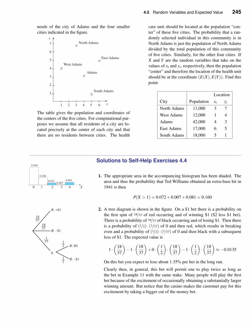
4.5 Random Variables and Expected Value 245
needs of the city of Adams and the four smaller
cities indicated in the figure.
1 2 3 4 5 6
7
6
5
4
3
2
1
West Adams
North Adams
East Adams
Adams
South Adams
x
y
The table gives the population and coordinates of
the centers of the five cities. For computational pur-
poses we assume that all residents of a city are lo-
cated precisely at the center of each city and that
there are no residents between cities. The health
care unit should be located at the population “cen-
ter” of these five cities. The probability that a ran-
domly selected individual in this community is in
North Adams is just the population of North Adams
divided by the total population of this community
of five cities. Similarly, for the other four cities. If
X and Y are the random variables that take on the
values of xi and yi, respectively, then the population
“center” and therefore the location of the health unit
should be at the coordinate (E(X),E(Y )). Find this
point.
Location
City Population xi yi
North Adams 11,000 3 7
West Adams 12,000 1 4
Adams 42,000 4 3
East Adams 17,000 6 5
South Adams 18,000 5 1
Solutions to Self-Help Exercises 4.4
1. The appropriate area in the accompanying histogram has been shaded. The
area and thus the probability that Ted Williams obtained an extra-base hit in
1941 is then
P(X > 1) = 0.072+0.007+0.081 = 0.160
2. A tree diagram is shown in the figure. On a $1 bet there is a probability on
the first spin of 18/37 of red occurring and of winning $1 ($2 less $1 bet).
There is a probability of 18/37 of black occurring and of losing $1. Then there
is a probability of (1/2) · (1/37) of 0 and then red, which results in breaking
even and a probability of (1/2) · (1/37) of 0 and then black with a subsequent
loss of $1. The expected value is
1 ·(
18
37
)
−1 ·(
18
37
)
+0 ·(
1
2
)
·(
18
37
)
−1 ·(
1
2
)
·(
18
37
)
≈−0.0135
On this bet you expect to lose about 1.35% per bet in the long run.
12
1837
R: +$1
R: $0
B: $1-
0
B: $1-
137
12
1837
Clearly then, in general, this bet will permit one to play twice as long as
the bet in Example 11 with the same stake. Many people will play the first
bet because of the excitement of occasionally obtaining a substantially larger
winning amount. But notice that the casino makes the customer pay for this
excitement by taking a bigger cut of the money bet.
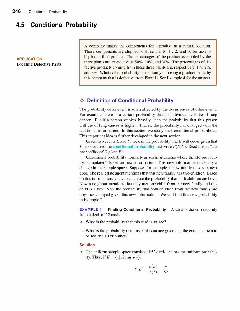
246 Chapter 4 Probability
4.5 Conditional Probability
APPLICATION
Locating Defective Parts
A company makes the components for a product at a central location.
These components are shipped to three plants, 1 , 2, and 3, for assem-
bly into a final product. The percentages of the product assembled by the
three plants are, respectively, 50%, 20%, and 30%. The percentages of de-
fective products coming from these three plants are, respectively, 1%, 2%,
and 3%. What is the probability of randomly choosing a product made by
this company that is defective from Plant 1? See Example 4 for the answer.
✧ Definition of Conditional Probability
The probability of an event is often affected by the occurrences of other events.
For example, there is a certain probability that an individual will die of lung
cancer. But if a person smokes heavily, then the probability that this person
will die of lung cancer is higher. That is, the probability has changed with the
additional information. In this section we study such conditional probabilities.
This important idea is further developed in the next section.
Given two events E and F , we call the probability that E will occur given that
F has occurred the conditional probability and write P(E|F). Read this as “the
probability of E given F .”
Conditional probability normally arises in situations where the old probabil-
ity is “updated” based on new information. This new information is usually a
change in the sample space. Suppose, for example, a new family moves in next
door. The real estate agent mentions that this new family has two children. Based
on this information, you can calculate the probability that both children are boys.
Now a neighbor mentions that they met one child from the new family and this
child is a boy. Now the probability that both children from the new family are
boys has changed given this new information. We will find this new probability
in Example 2.
EXAMPLE 1 Finding Conditional Probability A card is drawn randomly
from a deck of 52 cards.
a. What is the probability that this card is an ace?
b. What is the probability that this card is an ace given that the card is known to
be red and 10 or higher?
Solution
a. The uniform sample space consists of 52 cards and has the uniform probabil-
ity. Thus, if E = {x|x is an ace},
P(E) =n(E)
n(S)=
4
52
.
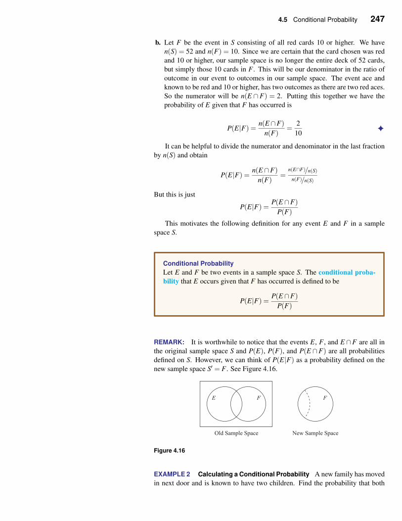
4.5 Conditional Probability 247
b. Let F be the event in S consisting of all red cards 10 or higher. We have
n(S) = 52 and n(F) = 10. Since we are certain that the card chosen was red
and 10 or higher, our sample space is no longer the entire deck of 52 cards,
but simply those 10 cards in F . This will be our denominator in the ratio of
outcome in our event to outcomes in our sample space. The event ace and
known to be red and 10 or higher, has two outcomes as there are two red aces.
So the numerator will be n(E ∩F) = 2. Putting this together we have the
probability of E given that F has occurred is
P(E|F) =n(E ∩F)
n(F)=
2
10✦
It can be helpful to divide the numerator and denominator in the last fraction
by n(S) and obtain
P(E|F) =n(E ∩F)
n(F)=
n(E∩F)/n(S)
n(F)/n(S)
But this is just
P(E|F) =P(E ∩F)
P(F)
This motivates the following definition for any event E and F in a sample
space S.
Conditional Probability
Let E and F be two events in a sample space S. The conditional proba-
bility that E occurs given that F has occurred is defined to be
P(E|F) =P(E ∩F)
P(F)
REMARK: It is worthwhile to notice that the events E, F , and E ∩F are all in
the original sample space S and P(E), P(F), and P(E ∩F) are all probabilities
defined on S. However, we can think of P(E|F) as a probability defined on the
new sample space S′ = F . See Figure 4.16.
Figure 4.16
EXAMPLE 2 Calculating a Conditional Probability A new family has moved
in next door and is known to have two children. Find the probability that both
248 Chapter 4 Probability
children are boys given that at least one is a boy. Assume that a boy is as likely
as a girl.
Solution Let E be the event that both children are a boy and F the event that
at least one is a boy. Then
S = {BB,BG,GB,GG},E = {BB},F = {BB,BG,GB},E ∩F = {BB}
and
P(E|F) =P(E ∩F)
P(F)=
1/4
3/4=
1
3✦
✧ The Product Rule
We will now see how to write P(E∩F) in terms of a product of two probabilities.
From the definition of conditional probability, we have
P(E|F) =P(E ∩F)
P(F), P(F |E) = P(F ∩E)
P(E)
if P(E)> 0 and P(F)> 0. Solving for P(E ∩F) and P(F ∩E), we obtain
P(E ∩F) = P(F)P(E|F), P(F ∩E) = P(E)P(F|E)
Since P(E ∩F) = P(F ∩E), it follows that
P(E ∩F) = P(F)P(E|F) = P(E)P(F|E)
This is called the product rule.
Product Rule
If E and F are two events in a sample space S with P(E)> 0 and P(F)> 0,
then
P(E ∩F) = P(F)P(E|F) = P(E)P(F|E)
EXAMPLE 3 Using the Product Rule Two bins contain transistors. The first
bin has 5 defective and 15 non-defective transistors while the second bin has 3
defective and 17 non-defective transistors. If the probability of picking either bin
is the same, what is the probability of picking the first bin and a good transistor?
Solution The sample space is S = {1D,1N,2D,2N} where the number refers
to picking the first or second bin and the letter refers to picking a defective (D) or
non-defective (N) transistor.
If E is the event “pick the first bin” and F is the event “pick a non-defective
transistor,” then E = {1D,1N} and F = {1N,2N}. The probability of picking a
non-defective transistor given that the first bin has been picked is the conditional
probability P(F|E) = 15/20. The event “picking the first bin and a non-defective
transistor” is E ∩F . From the product rule
P(E ∩F) = P(E)P(F|E) = 1
2· 15
20=
3
8✦
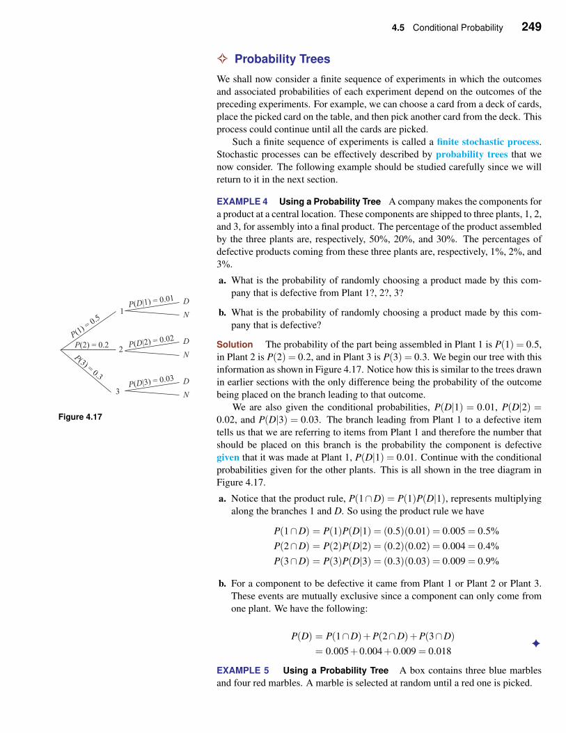
4.5 Conditional Probability 249
✧ Probability Trees
We shall now consider a finite sequence of experiments in which the outcomes
and associated probabilities of each experiment depend on the outcomes of the
preceding experiments. For example, we can choose a card from a deck of cards,
place the picked card on the table, and then pick another card from the deck. This
process could continue until all the cards are picked.
Such a finite sequence of experiments is called a finite stochastic process.
Stochastic processes can be effectively described by probability trees that we
now consider. The following example should be studied carefully since we will
return to it in the next section.
EXAMPLE 4 Using a Probability Tree A company makes the components for
a product at a central location. These components are shipped to three plants, 1, 2,
and 3, for assembly into a final product. The percentage of the product assembled
by the three plants are, respectively, 50%, 20%, and 30%. The percentages of
defective products coming from these three plants are, respectively, 1%, 2%, and
3%.
a. What is the probability of randomly choosing a product made by this com-
pany that is defective from Plant 1?, 2?, 3?
b. What is the probability of randomly choosing a product made by this com-
pany that is defective?
Solution The probability of the part being assembled in Plant 1 is P(1) = 0.5,
in Plant 2 is P(2) = 0.2, and in Plant 3 is P(3) = 0.3. We begin our tree with this
information as shown in Figure 4.17. Notice how this is similar to the trees drawn
in earlier sections with the only difference being the probability of the outcome
being placed on the branch leading to that outcome.
Figure 4.17We are also given the conditional probabilities, P(D|1) = 0.01, P(D|2) =
0.02, and P(D|3) = 0.03. The branch leading from Plant 1 to a defective item
tells us that we are referring to items from Plant 1 and therefore the number that
should be placed on this branch is the probability the component is defective
given that it was made at Plant 1, P(D|1) = 0.01. Continue with the conditional
probabilities given for the other plants. This is all shown in the tree diagram in
Figure 4.17.
a. Notice that the product rule, P(1∩D) = P(1)P(D|1), represents multiplying
along the branches 1 and D. So using the product rule we have
P(1∩D) = P(1)P(D|1) = (0.5)(0.01) = 0.005 = 0.5%
P(2∩D) = P(2)P(D|2) = (0.2)(0.02) = 0.004 = 0.4%
P(3∩D) = P(3)P(D|3) = (0.3)(0.03) = 0.009 = 0.9%
b. For a component to be defective it came from Plant 1 or Plant 2 or Plant 3.
These events are mutually exclusive since a component can only come from
one plant. We have the following:
P(D) = P(1∩D)+P(2∩D)+P(3∩D)
= 0.005+0.004+0.009 = 0.018✦
EXAMPLE 5 Using a Probability Tree A box contains three blue marbles
and four red marbles. A marble is selected at random until a red one is picked.
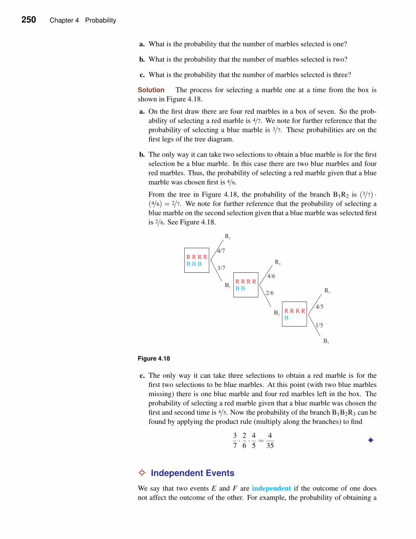
250 Chapter 4 Probability
a. What is the probability that the number of marbles selected is one?
b. What is the probability that the number of marbles selected is two?
c. What is the probability that the number of marbles selected is three?
Solution The process for selecting a marble one at a time from the box is
shown in Figure 4.18.
a. On the first draw there are four red marbles in a box of seven. So the prob-
ability of selecting a red marble is 4/7. We note for further reference that the
probability of selecting a blue marble is 3/7. These probabilities are on the
first legs of the tree diagram.
b. The only way it can take two selections to obtain a blue marble is for the first
selection be a blue marble. In this case there are two blue marbles and four
red marbles. Thus, the probability of selecting a red marble given that a blue
marble was chosen first is 4/6.
From the tree in Figure 4.18, the probability of the branch B1R2 is (3/7) ·(4/6) = 2/7. We note for further reference that the probability of selecting a
blue marble on the second selection given that a blue marble was selected first
is 2/6. See Figure 4.18.
Figure 4.18
c. The only way it can take three selections to obtain a red marble is for the
first two selections to be blue marbles. At this point (with two blue marbles
missing) there is one blue marble and four red marbles left in the box. The
probability of selecting a red marble given that a blue marble was chosen the
first and second time is 4/5. Now the probability of the branch B1B2R3 can be
found by applying the product rule (multiply along the branches) to find
3
7· 2
6· 4
5=
4
35✦
✧ Independent Events
We say that two events E and F are independent if the outcome of one does
not affect the outcome of the other. For example, the probability of obtaining a
4.5 Conditional Probability 251
head on a second flip of a coin is independent from what happened on the first
flip. This is intuitively clear since the coin cannot have any memory of what
happened on the first flip. Indeed the laws of physics determine the probability of
heads occurring. Thus for the probability of heads to be different on the second
flip the laws of physics must be different on the second flip. On the other hand,
if we are selecting cards one at time without replacement from a standard deck
of cards, the probability of selecting the queen of spades on the second draw
clearly depends on what happens on the first draw. If the queen of spades was
already picked, the probability of picking her on the second draw would be zero.
Thus drawing the queen of spades on the second draw without replacement is not
independent from drawing the queen of spades on the first draw.
That is, two events E and F are independent if
P(E|F) = P(E) and P(F |E) = P(F)
In words, the probability of E given that F has occurred is the same probability of
E if F had not occurred. Similarly, the probability of F given that E has occurred
is just the probability of F if E had not occurred.
Independent Events
Two events E and F are said to be independent if
P(E|F) = P(E) and P(F |E) = P(F)
We shall now obtain a result that is more convenient to apply when attempting
to determine if two events are independent. It will also be useful when finding
the probability that a series of independent events occurred.
If then two events E and F are independent, the previous comments together
with the product rule indicate that
P(E ∩F) = P(E|F)P(F) = P(E)P(F)
Now consider the case that P(E)> 0 and P(F)> 0. Assume that P(E∩F) =P(E)P(F), then
P(E|F) =P(E ∩F)
P(F)=
P(E)P(F)
P(F)= P(E)
P(F|E) = P(E ∩F)
P(E)=
P(E)P(F)
P(E)= P(F)
This discussion then yields the following theorem.
Independent Events Theorem
Let E and F be two events with P(E) > 0 and P(F) > 0. Then E and F
are independent if, and only if,
P(E ∩F) = P(E)P(F)
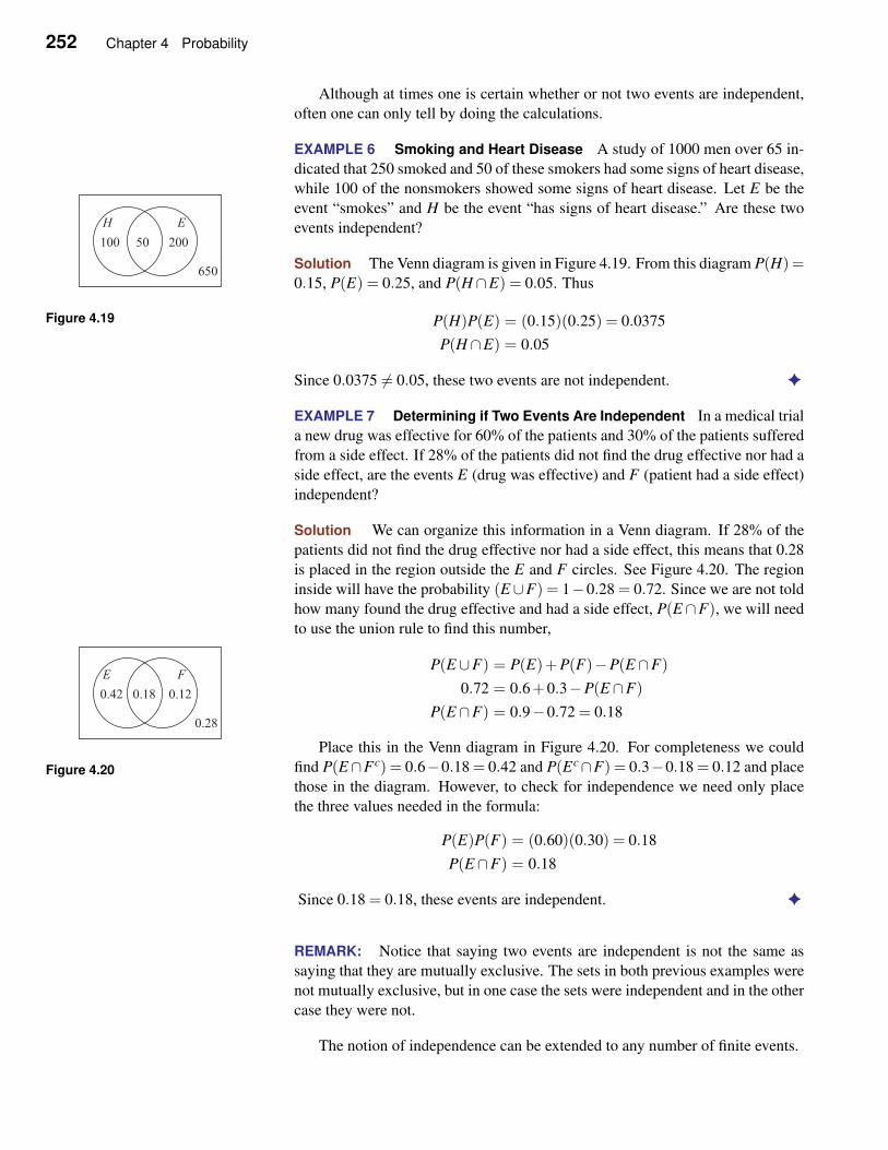
252 Chapter 4 Probability
Although at times one is certain whether or not two events are independent,
often one can only tell by doing the calculations.
EXAMPLE 6 Smoking and Heart Disease A study of 1000 men over 65 in-
dicated that 250 smoked and 50 of these smokers had some signs of heart disease,
while 100 of the nonsmokers showed some signs of heart disease. Let E be the
event “smokes” and H be the event “has signs of heart disease.” Are these two
events independent?
Solution The Venn diagram is given in Figure 4.19. From this diagram P(H) =0.15, P(E) = 0.25, and P(H ∩E) = 0.05. Thus
Figure 4.19 P(H)P(E) = (0.15)(0.25) = 0.0375
P(H ∩E) = 0.05
Since 0.0375 6= 0.05, these two events are not independent. ✦
EXAMPLE 7 Determining if Two Events Are Independent In a medical trial
a new drug was effective for 60% of the patients and 30% of the patients suffered
from a side effect. If 28% of the patients did not find the drug effective nor had a
side effect, are the events E (drug was effective) and F (patient had a side effect)
independent?
Solution We can organize this information in a Venn diagram. If 28% of the
patients did not find the drug effective nor had a side effect, this means that 0.28
is placed in the region outside the E and F circles. See Figure 4.20. The region
inside will have the probability (E ∪F) = 1−0.28 = 0.72. Since we are not told
how many found the drug effective and had a side effect, P(E ∩F), we will need
to use the union rule to find this number,
P(E ∪F) = P(E)+P(F)−P(E ∩F)
0.72 = 0.6+0.3−P(E ∩F)
P(E ∩F) = 0.9−0.72 = 0.18
Figure 4.20
Place this in the Venn diagram in Figure 4.20. For completeness we could
find P(E∩Fc) = 0.6−0.18 = 0.42 and P(Ec∩F) = 0.3−0.18 = 0.12 and place
those in the diagram. However, to check for independence we need only place
the three values needed in the formula:
P(E)P(F) = (0.60)(0.30) = 0.18
P(E ∩F) = 0.18
Since 0.18 = 0.18, these events are independent. ✦
REMARK: Notice that saying two events are independent is not the same as
saying that they are mutually exclusive. The sets in both previous examples were
not mutually exclusive, but in one case the sets were independent and in the other
case they were not.
The notion of independence can be extended to any number of finite events.
4.5 Conditional Probability 253
Independent Set of Events
A set of events {E1,E2, . . . ,En} is said to be independent if, for any k of
these events, the probability of the intersection of these k events is the
product of the probabilities of each of the k events. This must hold for any
k = 2,3, . . . ,n.
For example, for the set of events {E,F,G} to be independent all of the fol-
lowing must be true:
P(E ∩F) = P(E)P(F), P(E ∩G) = P(E)P(G)
P(F ∩G) = P(F)P(G), P(E ∩F ∩G) = P(E)P(F)P(G)
It is intuitively clear that if two events E and F are independent, then so also
are E and Fc, Ec and F , Ec and Fc. (See Exercises 52 and 53.) Similar statements
are true about a set of events.
EXAMPLE 8 Independent Events and Safety An aircraft has a system of
three computers, each independently able to exercise control of the flight. The
computers are considered 99.9% reliable during a routine flight. What is the
probability of having a failure of the control system during a routine flight?
Solution Let the events Ei, i = 1,2,3 be the three events given by the reliable
performance of respectively the first, second, and third computer. Since the set
of events {E1,E2,E3} is independent, so is the set of events {Ec1,E
c2,E
c3}. The
system will fail only if all three computers fail. Thus the probability of failure of
the system is given by
{Ec1 ∩Ec
2 ∩Ec3}= P(Ec
1)P(Ec2)P(E
c3) = (0.001)3
which, of course, is an extremely small number. ✦
EXAMPLE 9 Broken Elevators A building has three elevators. The chance
that elevator A is not working is 12%, the chance that elevator B is not working
is 15% and the chance that elevator C is not working is 9%. If these probabilities
are independent, what is the probability that exactly one elevator is not working?
Solution The probability that elevator A is not working but the other two
are working is (0.12)(0.85)(0.91). The probability that only elevator B is
working is (0.88)(0.15)(0.91) and only elevator C working has probability
(0.88)(0.85)(0.09) of occurring. The probability that exactly one does not work
is the sum of these three probabilities:
P = (0.12)(0.85)(0.91)+(0.88)(0.15)(0.91)+(0.88)(0.85)(0.09)
= 0.28026
✦
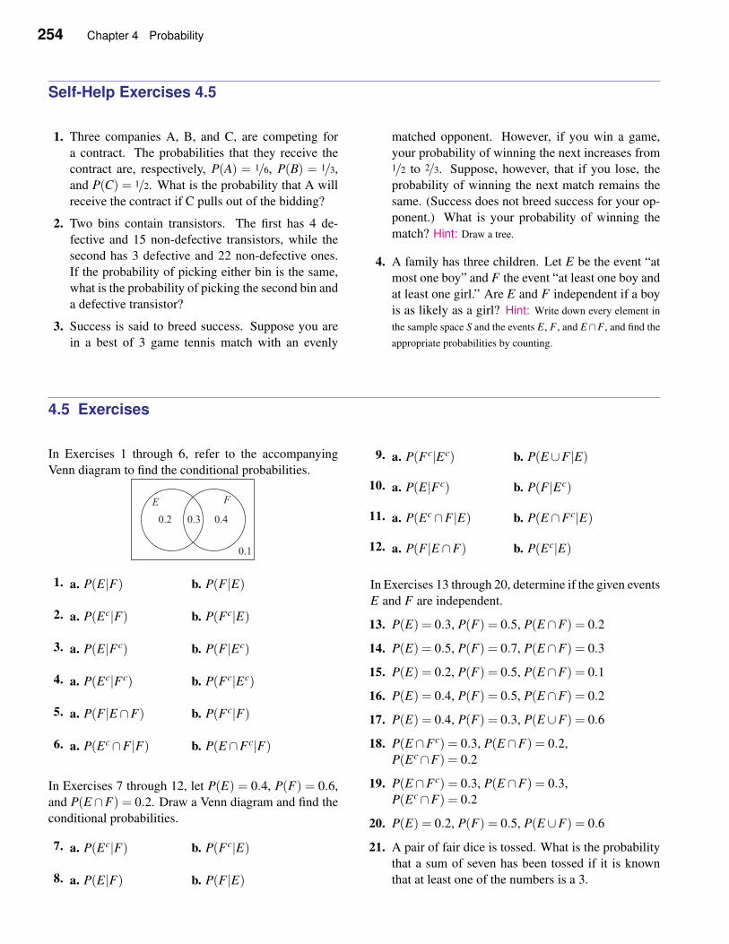
254 Chapter 4 Probability
Self-Help Exercises 4.5
1. Three companies A, B, and C, are competing for
a contract. The probabilities that they receive the
contract are, respectively, P(A) = 1/6, P(B) = 1/3,
and P(C) = 1/2. What is the probability that A will
receive the contract if C pulls out of the bidding?
2. Two bins contain transistors. The first has 4 de-
fective and 15 non-defective transistors, while the
second has 3 defective and 22 non-defective ones.
If the probability of picking either bin is the same,
what is the probability of picking the second bin and
a defective transistor?
3. Success is said to breed success. Suppose you are
in a best of 3 game tennis match with an evenly
matched opponent. However, if you win a game,
your probability of winning the next increases from1/2 to 2/3. Suppose, however, that if you lose, the
probability of winning the next match remains the
same. (Success does not breed success for your op-
ponent.) What is your probability of winning the
match? Hint: Draw a tree.
4. A family has three children. Let E be the event “at
most one boy” and F the event “at least one boy and
at least one girl.” Are E and F independent if a boy
is as likely as a girl? Hint: Write down every element in
the sample space S and the events E, F , and E∩F , and find the
appropriate probabilities by counting.
4.5 Exercises
In Exercises 1 through 6, refer to the accompanying
Venn diagram to find the conditional probabilities.
1. a. P(E|F) b. P(F|E)
2. a. P(Ec|F) b. P(Fc|E)
3. a. P(E|Fc) b. P(F|Ec)
4. a. P(Ec|Fc) b. P(Fc|Ec)
5. a. P(F|E ∩F) b. P(Fc|F)
6. a. P(Ec∩F |F) b. P(E ∩Fc|F)
In Exercises 7 through 12, let P(E) = 0.4, P(F) = 0.6,
and P(E ∩F) = 0.2. Draw a Venn diagram and find the
conditional probabilities.
7. a. P(Ec|F) b. P(Fc|E)
8. a. P(E|F) b. P(F|E)
9. a. P(Fc|Ec) b. P(E ∪F |E)
10. a. P(E|Fc) b. P(F|Ec)
11. a. P(Ec∩F |E) b. P(E ∩Fc|E)
12. a. P(F|E ∩F) b. P(Ec|E)
In Exercises 13 through 20, determine if the given events
E and F are independent.
13. P(E) = 0.3, P(F) = 0.5, P(E ∩F) = 0.2
14. P(E) = 0.5, P(F) = 0.7, P(E ∩F) = 0.3
15. P(E) = 0.2, P(F) = 0.5, P(E ∩F) = 0.1
16. P(E) = 0.4, P(F) = 0.5, P(E ∩F) = 0.2
17. P(E) = 0.4, P(F) = 0.3, P(E ∪F) = 0.6
18. P(E ∩Fc) = 0.3, P(E ∩F) = 0.2,
P(Ec∩F) = 0.2
19. P(E ∩Fc) = 0.3, P(E ∩F) = 0.3,
P(Ec∩F) = 0.2
20. P(E) = 0.2, P(F) = 0.5, P(E ∪F) = 0.6
21. A pair of fair dice is tossed. What is the probability
that a sum of seven has been tossed if it is known
that at least one of the numbers is a 3.
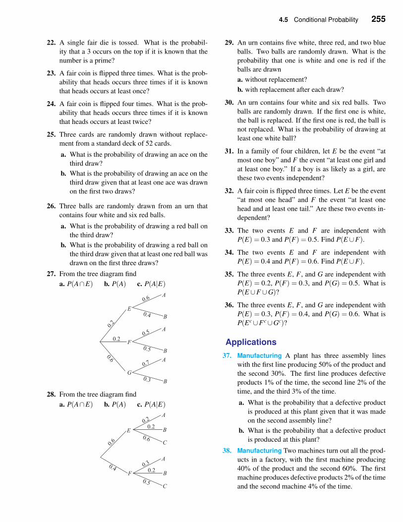
4.5 Conditional Probability 255
22. A single fair die is tossed. What is the probabil-
ity that a 3 occurs on the top if it is known that the
number is a prime?
23. A fair coin is flipped three times. What is the prob-
ability that heads occurs three times if it is known
that heads occurs at least once?
24. A fair coin is flipped four times. What is the prob-
ability that heads occurs three times if it is known
that heads occurs at least twice?
25. Three cards are randomly drawn without replace-
ment from a standard deck of 52 cards.
a. What is the probability of drawing an ace on the
third draw?
b. What is the probability of drawing an ace on the
third draw given that at least one ace was drawn
on the first two draws?
26. Three balls are randomly drawn from an urn that
contains four white and six red balls.
a. What is the probability of drawing a red ball on
the third draw?
b. What is the probability of drawing a red ball on
the third draw given that at least one red ball was
drawn on the first three draws?
27. From the tree diagram find
a. P(A∩E) b. P(A) c. P(A|E)
28. From the tree diagram find
a. P(A∩E) b. P(A) c. P(A|E)
29. An urn contains five white, three red, and two blue
balls. Two balls are randomly drawn. What is the
probability that one is white and one is red if the
balls are drawn
a. without replacement?
b. with replacement after each draw?
30. An urn contains four white and six red balls. Two
balls are randomly drawn. If the first one is white,
the ball is replaced. If the first one is red, the ball is
not replaced. What is the probability of drawing at
least one white ball?
31. In a family of four children, let E be the event “at
most one boy” and F the event “at least one girl and
at least one boy.” If a boy is as likely as a girl, are
these two events independent?
32. A fair coin is flipped three times. Let E be the event
“at most one head” and F the event “at least one
head and at least one tail.” Are these two events in-
dependent?
33. The two events E and F are independent with
P(E) = 0.3 and P(F) = 0.5. Find P(E ∪F).
34. The two events E and F are independent with
P(E) = 0.4 and P(F) = 0.6. Find P(E ∪F).
35. The three events E, F , and G are independent with
P(E) = 0.2, P(F) = 0.3, and P(G) = 0.5. What is
P(E ∪F ∪G)?
36. The three events E, F , and G are independent with
P(E) = 0.3, P(F) = 0.4, and P(G) = 0.6. What is
P(Ec∪Fc∪Gc)?
Applications
37. Manufacturing A plant has three assembly lines
with the first line producing 50% of the product and
the second 30%. The first line produces defective
products 1% of the time, the second line 2% of the
time, and the third 3% of the time.
a. What is the probability that a defective product
is produced at this plant given that it was made
on the second assembly line?
b. What is the probability that a defective product
is produced at this plant?
38. Manufacturing Two machines turn out all the prod-
ucts in a factory, with the first machine producing
40% of the product and the second 60%. The first
machine produces defective products 2% of the time
and the second machine 4% of the time.
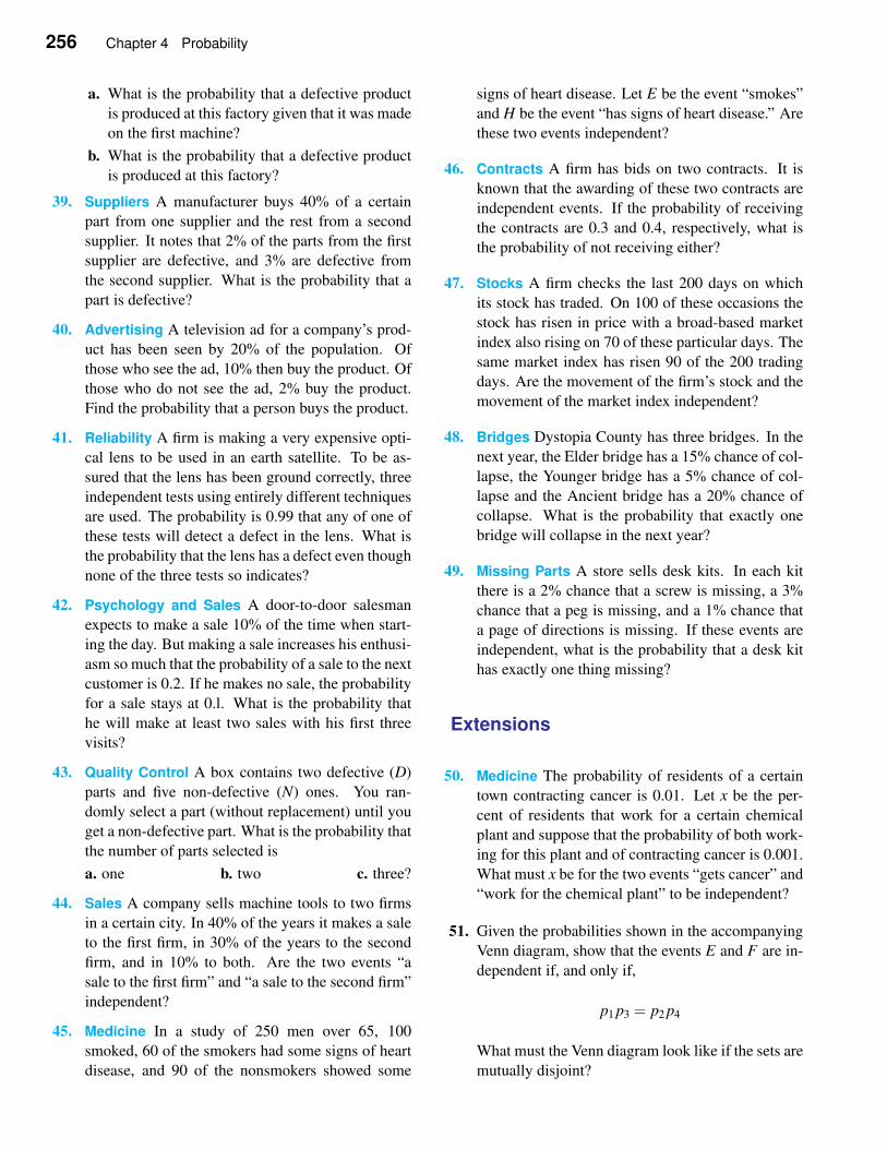
256 Chapter 4 Probability
a. What is the probability that a defective product
is produced at this factory given that it was made
on the first machine?
b. What is the probability that a defective product
is produced at this factory?
39. Suppliers A manufacturer buys 40% of a certain
part from one supplier and the rest from a second
supplier. It notes that 2% of the parts from the first
supplier are defective, and 3% are defective from
the second supplier. What is the probability that a
part is defective?
40. Advertising A television ad for a company’s prod-
uct has been seen by 20% of the population. Of
those who see the ad, 10% then buy the product. Of
those who do not see the ad, 2% buy the product.
Find the probability that a person buys the product.
41. Reliability A firm is making a very expensive opti-
cal lens to be used in an earth satellite. To be as-
sured that the lens has been ground correctly, three
independent tests using entirely different techniques
are used. The probability is 0.99 that any of one of
these tests will detect a defect in the lens. What is
the probability that the lens has a defect even though
none of the three tests so indicates?
42. Psychology and Sales A door-to-door salesman
expects to make a sale 10% of the time when start-
ing the day. But making a sale increases his enthusi-
asm so much that the probability of a sale to the next
customer is 0.2. If he makes no sale, the probability
for a sale stays at 0.l. What is the probability that
he will make at least two sales with his first three
visits?
43. Quality Control A box contains two defective (D)
parts and five non-defective (N) ones. You ran-
domly select a part (without replacement) until you
get a non-defective part. What is the probability that
the number of parts selected is
a. one b. two c. three?
44. Sales A company sells machine tools to two firms
in a certain city. In 40% of the years it makes a sale
to the first firm, in 30% of the years to the second
firm, and in 10% to both. Are the two events “a
sale to the first firm” and “a sale to the second firm”
independent?
45. Medicine In a study of 250 men over 65, 100
smoked, 60 of the smokers had some signs of heart
disease, and 90 of the nonsmokers showed some
signs of heart disease. Let E be the event “smokes”
and H be the event “has signs of heart disease.” Are
these two events independent?
46. Contracts A firm has bids on two contracts. It is
known that the awarding of these two contracts are
independent events. If the probability of receiving
the contracts are 0.3 and 0.4, respectively, what is
the probability of not receiving either?
47. Stocks A firm checks the last 200 days on which
its stock has traded. On 100 of these occasions the
stock has risen in price with a broad-based market
index also rising on 70 of these particular days. The
same market index has risen 90 of the 200 trading
days. Are the movement of the firm’s stock and the
movement of the market index independent?
48. Bridges Dystopia County has three bridges. In the
next year, the Elder bridge has a 15% chance of col-
lapse, the Younger bridge has a 5% chance of col-
lapse and the Ancient bridge has a 20% chance of
collapse. What is the probability that exactly one
bridge will collapse in the next year?
49. Missing Parts A store sells desk kits. In each kit
there is a 2% chance that a screw is missing, a 3%
chance that a peg is missing, and a 1% chance that
a page of directions is missing. If these events are
independent, what is the probability that a desk kit
has exactly one thing missing?
Extensions
50. Medicine The probability of residents of a certain
town contracting cancer is 0.01. Let x be the per-
cent of residents that work for a certain chemical
plant and suppose that the probability of both work-
ing for this plant and of contracting cancer is 0.001.
What must x be for the two events “gets cancer” and
“work for the chemical plant” to be independent?
51. Given the probabilities shown in the accompanying
Venn diagram, show that the events E and F are in-
dependent if, and only if,
p1 p3 = p2 p4
What must the Venn diagram look like if the sets are
mutually disjoint?
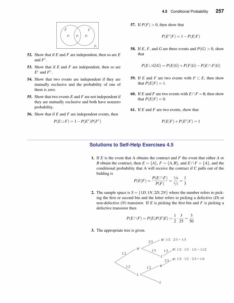
4.5 Conditional Probability 257
52. Show that if E and F are independent, then so are E
and Fc.
53. Show that if E and F are independent, then so are
Ec and Fc.
54. Show that two events are independent if they are
mutually exclusive and the probability of one of
them is zero.
55. Show that two events E and F are not independent if
they are mutually exclusive and both have nonzero
probability.
56. Show that if E and F are independent events, then
P(E ∪F) = 1−P(Ec)P(Fc)
57. If P(F)> 0, then show that
P(Ec|F) = 1−P(E|F)
58. If E, F , and G are three events and P(G)> 0, show
that
P(E ∪G|G) = P(E|G)+P(F|G)−P(E ∩F |G)
59. If E and F are two events with F ⊂ E, then show
that P(E|F) = 1.
60. If E and F are two events with E∩F = /0, then show
that P(E|F) = 0.
61. If E and F are two events, show that
P(E|F)+P(Ec|F) = 1
Solutions to Self-Help Exercises 4.5
1. If E is the event that A obtains the contract and F the event that either A or
B obtain the contract, then E = {A}, F = {A,B}, and E ∩F = {A}, and the
conditional probability that A will receive the contract if C pulls out of the
bidding is
P(E|F) =P(E ∩F)
P(F)=
1/6
1/2=
1
3
2. The sample space is S = {1D,1N,2D,2N} where the number refers to pick-
ing the first or second bin and the letter refers to picking a defective (D) or
non-defective (N) transistor. If E is picking the first bin and F is picking a
defective transistor then
P(E ∩F) = P(E)P(F|E) = 1
2· 3
25=
3
50
3. The appropriate tree is given.
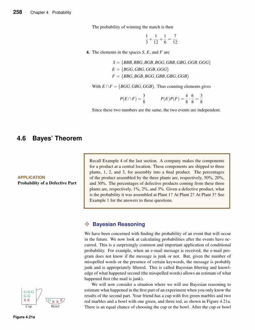
258 Chapter 4 Probability
The probability of winning the match is then
1
3+
1
12+
1
6=
7
12
4. The elements in the spaces S, E, and F are
S = {BBB,BBG,BGB,BGG,GBB,GBG,GGB,GGG}E = {BGG,GBG,GGB,GGG}F = {BBG,BGB,BGG,GBB,GBG,GGB}
With E ∩F = {BGG,GBG,GGB}. Thus counting elements gives
P(E ∩F) =3
8P(E)P(F) =
4
8· 6
8=
3
8
Since these two numbers are the same, the two events are independent.
4.6 Bayes’ Theorem
APPLICATION
Probability of a Defective Part
Recall Example 4 of the last section. A company makes the components
for a product at a central location. These components are shipped to three
plants, 1, 2, and 3, for assembly into a final product. The percentages
of the product assembled by the three plants are, respectively, 50%, 20%,
and 30%. The percentages of defective products coming from these three
plants are, respectively, 1%, 2%, and 3%. Given a defective product, what
is the probability it was assembled at Plant 1? At Plant 2? At Plant 3? See
Example 1 for the answers to these questions.
✧ Bayesian Reasoning
We have been concerned with finding the probability of an event that will occur
in the future. We now look at calculating probabilities after the events have oc-
curred. This is a surprisingly common and important application of conditional
probability. For example, when an e-mail message is received, the e-mail pro-
gram does not know if the message is junk or not. But, given the number of
misspelled words or the presence of certain keywords, the message is probably
junk and is appropriately filtered. This is called Bayesian filtering and knowl-
edge of what happened second (the misspelled words) allows an estimate of what
happened first (the mail is junk).
We will now consider a situation where we will use Bayesian reasoning to
estimate what happened in the first part of an experiment when you only know the
results of the second part. Your friend has a cup with five green marbles and two
red marbles and a bowl with one green, and three red, as shown in Figure 4.21a.
There is an equal chance of choosing the cup or the bowl. After the cup or bowl
Figure 4.21a
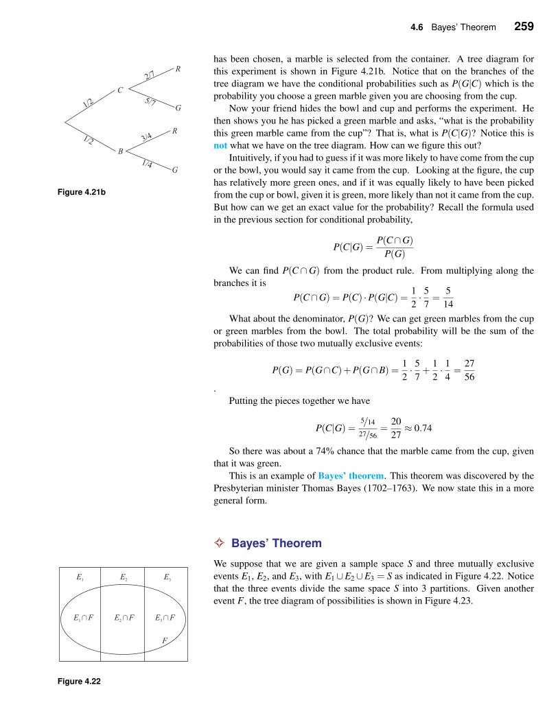
4.6 Bayes’ Theorem 259
has been chosen, a marble is selected from the container. A tree diagram for
this experiment is shown in Figure 4.21b. Notice that on the branches of the
tree diagram we have the conditional probabilities such as P(G|C) which is the
probability you choose a green marble given you are choosing from the cup.
Now your friend hides the bowl and cup and performs the experiment. He
then shows you he has picked a green marble and asks, “what is the probability
this green marble came from the cup”? That is, what is P(C|G)? Notice this is
not what we have on the tree diagram. How can we figure this out?
Intuitively, if you had to guess if it was more likely to have come from the cup
or the bowl, you would say it came from the cup. Looking at the figure, the cup
Figure 4.21bhas relatively more green ones, and if it was equally likely to have been picked
from the cup or bowl, given it is green, more likely than not it came from the cup.
But how can we get an exact value for the probability? Recall the formula used
in the previous section for conditional probability,
P(C|G) =P(C∩G)
P(G)
We can find P(C ∩G) from the product rule. From multiplying along the
branches it is
P(C∩G) = P(C) ·P(G|C) =1
2· 5
7=
5
14
What about the denominator, P(G)? We can get green marbles from the cup
or green marbles from the bowl. The total probability will be the sum of the
probabilities of those two mutually exclusive events:
P(G) = P(G∩C)+P(G∩B) =1
2· 5
7+
1
2· 1
4=
27
56.
Putting the pieces together we have
P(C|G) =5/14
27/56=
20
27≈ 0.74
So there was about a 74% chance that the marble came from the cup, given
that it was green.
This is an example of Bayes’ theorem. This theorem was discovered by the
Presbyterian minister Thomas Bayes (1702–1763). We now state this in a more
general form.
✧ Bayes’ Theorem
We suppose that we are given a sample space S and three mutually exclusive
events E1, E2, and E3, with E1∪E2∪E3 = S as indicated in Figure 4.22. Notice
Figure 4.22
that the three events divide the same space S into 3 partitions. Given another
event F , the tree diagram of possibilities is shown in Figure 4.23.
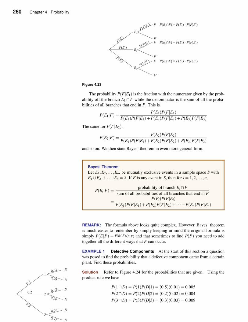
260 Chapter 4 Probability
Figure 4.23
The probability P(F|E1) is the fraction with the numerator given by the prob-
ability off the branch E1 ∩F while the denominator is the sum of all the proba-
bilities of all branches that end in F . This is
P(E1|F) =P(E1)P(F|E1)
P(E1)P(F|E1)+P(E2)P(F|E2)+P(E3)P(F|E3)
The same for P(F|E2).
P(E2|F) =P(E2)P(F|E2)
P(E1)P(F|E1)+P(E2)P(F|E2)+P(E3)P(F|E3)
and so on. We then state Bayes’ theorem in even more general form.
Bayes’ Theorem
Let E1,E2, . . . ,En, be mutually exclusive events in a sample space S with
E1∪E2∪ . . .∪En = S. If F is any event in S, then for i = 1,2, . . . ,n,
P(Ei|F) =probability of branch Ei∩F
sum of all probabilities of all branches that end in F
=P(Ei)P(F|Ei)
P(E1)P(F|E1)+P(E2)P(F|E2)+ · · ·+P(En)P(F|En)
REMARK: The formula above looks quite complex. However, Bayes’ theorem
is much easier to remember by simply keeping in mind the original formula is
simply P(E|F) = P(E∩F)/P(F) and that sometimes to find P(F) you need to add
together all the different ways that F can occur.
EXAMPLE 1 Defective Components At the start of this section a question
was posed to find the probability that a defective component came from a certain
plant. Find these probabilities.
Solution Refer to Figure 4.24 for the probabilities that are given. Using the
product rule we have
P(1∩D) = P(1)P(D|1) = (0.5)(0.01) = 0.005
P(2∩D) = P(2)P(D|2) = (0.2)(0.02) = 0.004
P(3∩D) = P(3)P(D|3) = (0.3)(0.03) = 0.009
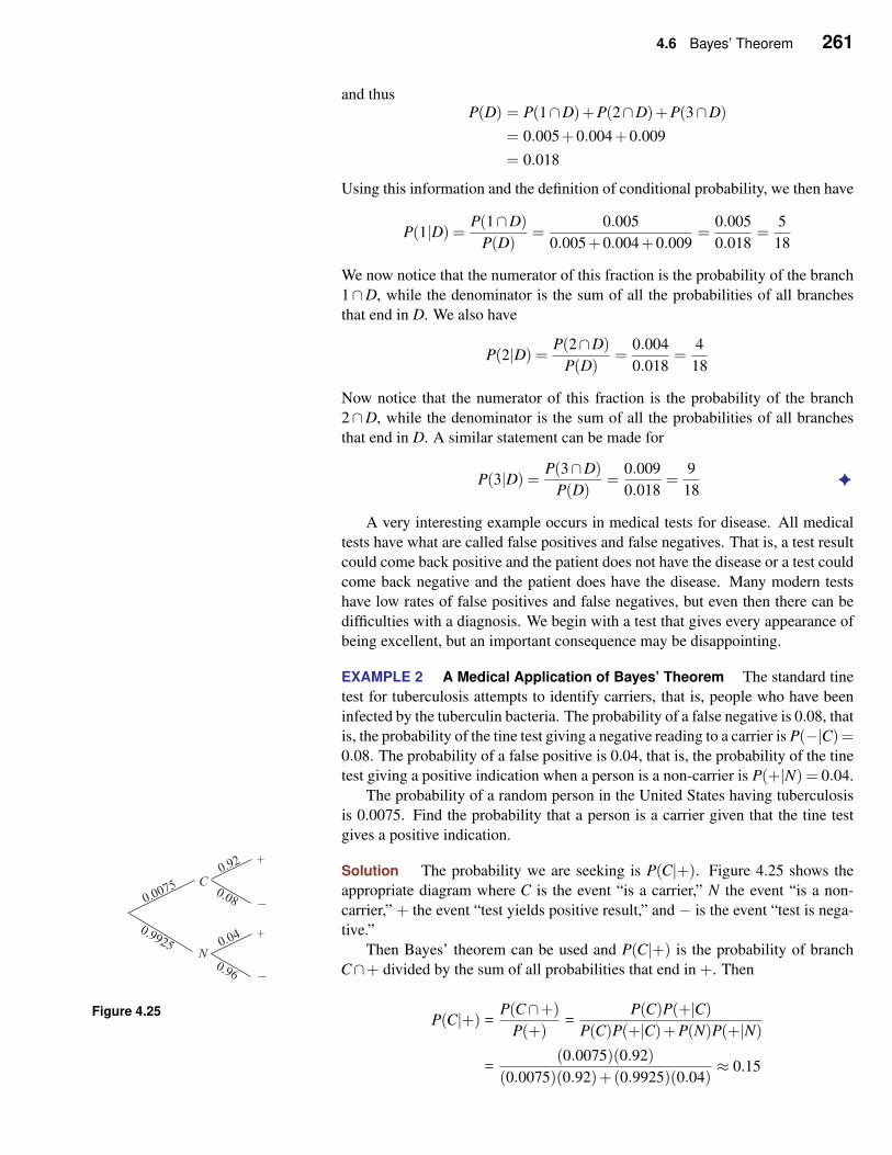
4.6 Bayes’ Theorem 261
and thusP(D) = P(1∩D)+P(2∩D)+P(3∩D)
= 0.005+0.004+0.009
= 0.018
Using this information and the definition of conditional probability, we then have
P(1|D) =P(1∩D)
P(D)=
0.005
0.005+0.004+0.009=
0.005
0.018=
5
18
We now notice that the numerator of this fraction is the probability of the branch
1∩D, while the denominator is the sum of all the probabilities of all branches
that end in D. We also have
P(2|D) =P(2∩D)
P(D)=
0.004
0.018=
4
18
Now notice that the numerator of this fraction is the probability of the branch
2∩D, while the denominator is the sum of all the probabilities of all branches
that end in D. A similar statement can be made for
P(3|D) =P(3∩D)
P(D)=
0.009
0.018=
9
18✦
A very interesting example occurs in medical tests for disease. All medical
tests have what are called false positives and false negatives. That is, a test result
could come back positive and the patient does not have the disease or a test could
come back negative and the patient does have the disease. Many modern tests
have low rates of false positives and false negatives, but even then there can be
difficulties with a diagnosis. We begin with a test that gives every appearance of
being excellent, but an important consequence may be disappointing.
EXAMPLE 2 A Medical Application of Bayes’ Theorem The standard tine
test for tuberculosis attempts to identify carriers, that is, people who have been
infected by the tuberculin bacteria. The probability of a false negative is 0.08, that
is, the probability of the tine test giving a negative reading to a carrier is P(−|C)=0.08. The probability of a false positive is 0.04, that is, the probability of the tine
test giving a positive indication when a person is a non-carrier is P(+|N) = 0.04.
The probability of a random person in the United States having tuberculosis
is 0.0075. Find the probability that a person is a carrier given that the tine test
gives a positive indication.
Solution The probability we are seeking is P(C|+). Figure 4.25 shows the
appropriate diagram where C is the event “is a carrier,” N the event “is a non-
carrier,” + the event “test yields positive result,” and − is the event “test is nega-
tive.”
Figure 4.25
Then Bayes’ theorem can be used and P(C|+) is the probability of branch
C∩+ divided by the sum of all probabilities that end in +. Then
P(C|+) =P(C∩+)
P(+)=
P(C)P(+|C)
P(C)P(+|C)+P(N)P(+|N)
=(0.0075)(0.92)
(0.0075)(0.92)+(0.9925)(0.04)≈ 0.15
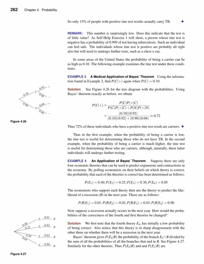
262 Chapter 4 Probability
So only 15% of people with positive tine test results actually carry TB. ✦
REMARK: This number is surprisingly low. Does this indicate that the test is
of little value? As Self-Help Exercise 1 will show, a person whose tine test is
negative has a probability of 0.999 of not having tuberculosis. Such an individual
can feel safe. The individuals whose tine test is positive are probably all right
also but will need to undergo further tests, such as a chest x-ray.
In some areas of the United States the probability of being a carrier can be
as high as 0.10. The following example examines the tine test under these condi-
tions.
EXAMPLE 3 A Medical Application of Bayes’ Theorem Using the informa-
tion found in Example 2, find P(C|+) again when P(C) = 0.10.
Solution See Figure 4.26 for the tree diagram with the probabilities. Using
Bayes’ theorem exactly as before, we obtain
Figure 4.26
P(C|+) =P(C)P(+|C)
P(C)P(+|C)+P(N)P(+|N)
=(0.10)(0.92)
(0.10)(0.92)+(0.90)(0.04)≈ 0.72
Thus 72% of these individuals who have a positive tine test result are carriers. ✦
Thus in the first example, when the probability of being a carrier is low,
the tine test is useful for determining those who do not have TB. In the second
example, when the probability of being a carrier is much higher, the tine test
is useful for determining those who are carriers, although, naturally, these latter
individuals will undergo further testing.
EXAMPLE 4 An Application of Bayes’ Theorem Suppose there are only
four economic theories that can be used to predict expansions and contractions in
the economy. By polling economists on their beliefs on which theory is correct,
the probability that each of the theories is correct has been determined as follows:
P(E1) = 0.40,P(E2) = 0.25,P(E3) = 0.30,P(E4) = 0.05
The economists who support each theory then use the theory to predict the like-
lihood of a recession (R) in the next year. These are as follows:
P(R|E1) = 0.01,P(R|E2) = 0.02,P(R|E3) = 0.03,P(R|E4) = 0.90
Now suppose a recession actually occurs in the next year. How would the proba-
bilities of the correctness of the fourth and first theories be changed?
Solution We first note that the fourth theory E4, has initially a low probability
of being correct. Also notice that this theory is in sharp disagreement with the
other three on whether there will be a recession in the next year.
Bayes’ theorem gives P(E4|R) the probability of the branch E4∩R divided by
the sum of all the probabilities of all the branches that end in R. See Figure 4.27.
Similarly for the other theories. Thus P(E4|R) and and P(E1|R) are
Figure 4.27
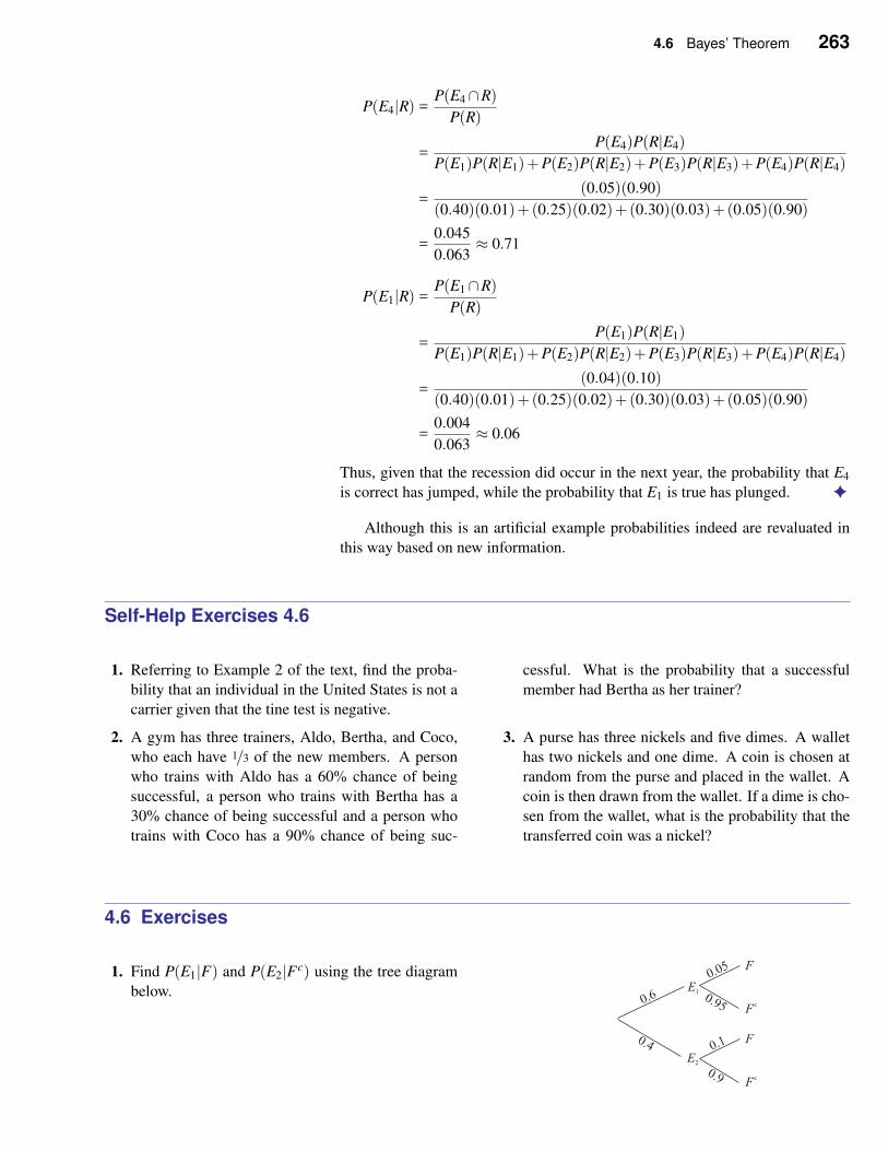
4.6 Bayes’ Theorem 263
P(E4|R) =P(E4∩R)
P(R)
=P(E4)P(R|E4)
P(E1)P(R|E1)+P(E2)P(R|E2)+P(E3)P(R|E3)+P(E4)P(R|E4)
=(0.05)(0.90)
(0.40)(0.01)+(0.25)(0.02)+(0.30)(0.03)+(0.05)(0.90)
=0.045
0.063≈ 0.71
P(E1|R) =P(E1∩R)
P(R)
=P(E1)P(R|E1)
P(E1)P(R|E1)+P(E2)P(R|E2)+P(E3)P(R|E3)+P(E4)P(R|E4)
=(0.04)(0.10)
(0.40)(0.01)+(0.25)(0.02)+(0.30)(0.03)+(0.05)(0.90)
=0.004
0.063≈ 0.06
Thus, given that the recession did occur in the next year, the probability that E4
is correct has jumped, while the probability that E1 is true has plunged. ✦
Although this is an artificial example probabilities indeed are revaluated in
this way based on new information.
Self-Help Exercises 4.6
1. Referring to Example 2 of the text, find the proba-
bility that an individual in the United States is not a
carrier given that the tine test is negative.
2. A gym has three trainers, Aldo, Bertha, and Coco,
who each have 1/3 of the new members. A person
who trains with Aldo has a 60% chance of being
successful, a person who trains with Bertha has a
30% chance of being successful and a person who
trains with Coco has a 90% chance of being suc-
cessful. What is the probability that a successful
member had Bertha as her trainer?
3. A purse has three nickels and five dimes. A wallet
has two nickels and one dime. A coin is chosen at
random from the purse and placed in the wallet. A
coin is then drawn from the wallet. If a dime is cho-
sen from the wallet, what is the probability that the
transferred coin was a nickel?
4.6 Exercises
1. Find P(E1|F) and P(E2|Fc) using the tree diagram
below.
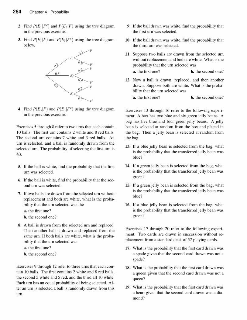
264 Chapter 4 Probability
2. Find P(E1|Fc) and P(E2|F) using the tree diagram
in the previous exercise.
3. Find P(E1|F) and P(E1|Fc) using the tree diagram
below.
4. Find P(E3|F) and P(E3|Fc) using the tree diagram
in the previous exercise.
Exercises 5 through 8 refer to two urns that each contain
10 balls. The first urn contains 2 white and 8 red balls.
The second urn contains 7 white and 3 red balls. An
urn is selected, and a ball is randomly drawn from the
selected urn. The probability of selecting the first urn is2/3.
5. If the ball is white, find the probability that the first
urn was selected.
6. If the ball is white, find the probability that the sec-
ond urn was selected.
7. If two balls are drawn from the selected urn without
replacement and both are white, what is the proba-
bility that the urn selected was the
a. the first one?
b. the second one?
8. A ball is drawn from the selected urn and replaced.
Then another ball is drawn and replaced from the
same urn. If both balls are white, what is the proba-
bility that the urn selected was
a. the first one?
b. the second one?
Exercises 9 through 12 refer to three urns that each con-
tain 10 balls. The first contains 2 white and 8 red balls,
the second 5 white and 5 red, and the third all 10 white.
Each urn has an equal probability of being selected. Af-
ter an urn is selected a ball is randomly drawn from this
urn.
9. If the ball drawn was white, find the probability that
the first urn was selected.
10. If the ball drawn was white, find the probability that
the third urn was selected.
11. Suppose two balls are drawn from the selected urn
without replacement and both are white. What is the
probability that the urn selected was
a. the first one? b. the second one?
12. Now a ball is drawn, replaced, and then another
drawn. Suppose both are white. What is the proba-
bility that the urn selected was
a. the first one? b. the second one?
Exercises 13 through 16 refer to the following experi-
ment: A box has two blue and six green jelly beans. A
bag has five blue and four green jelly beans. A jelly
bean is selected at random from the box and placed in
the bag. Then a jelly bean is selected at random from
the bag.
13. If a blue jelly bean is selected from the bag, what
is the probability that the transferred jelly bean was
blue?
14. If a green jelly bean is selected from the bag, what
is the probability that the transferred jelly bean was
green?
15. If a green jelly bean is selected from the bag, what
is the probability that the transferred jelly bean was
blue?
16. If a blue jelly bean is selected from the bag, what
is the probability that the transferred jelly bean was
green?
Exercises 17 through 20 refer to the following experi-
ment: Two cards are drawn in succession without re-
placement from a standard deck of 52 playing cards.
17. What is the probability that the first card drawn was
a spade given that the second card drawn was not a
spade?
18. What is the probability that the first card drawn was
a queen given that the second card drawn was not a
queen?
19. What is the probability that the first card drawn was
a heart given that the second card drawn was a dia-
mond?
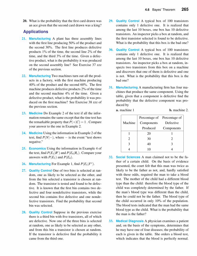
4.6 Bayes’ Theorem 265
20. What is the probability that the first card drawn was
an ace given that the second card drawn was a king?
Applications
21. Manufacturing A plant has three assembly lines
with the first line producing 50% of the product and
the second 30%. The first line produces defective
products 1% of the time, the second line 2% of the
time, and the third 3% of the time. Given a defec-
tive product, what is the probability it was produced
on the second assembly line? See Exercise 37 zzz
of the previous section.
22. Manufacturing Two machines turn out all the prod-
ucts in a factory, with the first machine producing
40% of the product and the second 60%. The first
machine produces defective products 2% of the time
and the second machine 4% of the time. Given a
defective product, what is the probability it was pro-
duced on the first machine? See Exercise 38 zzz of
the previous section.
23. Medicine Do Example 2 of the text if all the infor-
mation remains the same except that the tine test has
the remarkable property that P(+|C) = 1 . Compare
your answer to the one in Example 2.
24. Medicine Using the information in Example 2 of the
text, find P(N|−), where − is the event “test shows
negative.”
25. Economics Using the information in Example 4 of
the text, find P(E1|Rc) and P(E4|Rc). Compare your
answers with P(E1) and P(E4).
26. Manufacturing For Example 1, find P(E1|Fc).
27. Quality Control One of two bins is selected at ran-
dom, one as likely to be selected as the other, and
from the bin selected a transistor is chosen at ran-
dom. The transistor is tested and found to be defec-
tive. It is known that the first bin contains two de-
fective and four nondefective transistors, while the
second bin contains five defective and one nonde-
fective transistors. Find the probability that second
bin was selected.
28. Quality Control Suppose in the previous exercise
there is a third bin with five transistors, all of which
are defective. Now one of the three bins is selected
at random, one as likely to be selected as any other,
and from this bin a transistor is chosen at random.
If the transistor is defective find the probability it
came from the third one.
29. Quality Control A typical box of 100 transistors
contains only 1 defective one. It is realized that
among the last 10 boxes, one box has 10 defective
transistors. An inspector picks a box at random, and
the first transistor selected is found to be defective.
What is the probability that this box is the bad one?
30. Quality Control A typical box of 100 transistors
contains only 1 defective one. It is realized that
among the last 10 boxes, one box has 10 defective
transistors. An inspector picks a box at random, in-
spects two transistors from this box on a machine
and discovers that one of them is defective and one
is not. What is the probability that this box is the
bad one?
31. Manufacturing A manufacturing firm has four ma-
chines that produce the same component. Using the
table, given that a component is defective find the
probability that the defective component was pro-
duced by
a. machine 1 b. machine 2.
Percentage of Percentage of
Machine Components Defective
Produced Components
1 20 1
2 30 2
3 40 3
4 10 4
32. Social Sciences A man claimed not to be the fa-
ther of a certain child. On the basis of evidence
presented, the court felt that this man was twice as
likely to be the father as not, and, hardly satisfied
with these odds, required the man to take a blood
test. The mother of the child had a different blood
type than the child: therefore the blood type of the
child was completely determined by the father. If
the man’s blood type was different than the child,
then he could not be the father. The blood type of
the child occurred in only 10% of the population.
The blood tests indicated that the man had the same
blood type as the child. What is the probability that
the man is the father?
33. Medical Diagnosis A physician examines a patient
and, on the basis of the symptoms, determines that
he may have one of four diseases; the probability of
each is given in the table. She orders a blood test,
which indicates that the blood is perfectly normal.
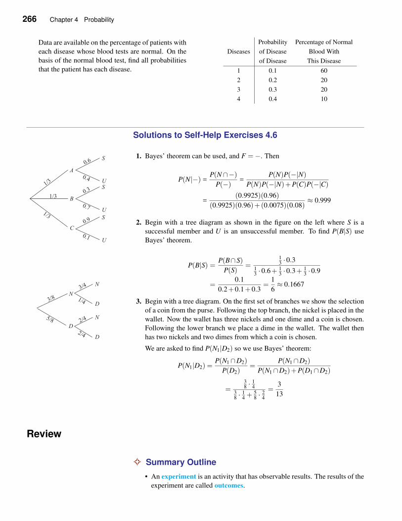
266 Chapter 4 Probability
Data are available on the percentage of patients with
each disease whose blood tests are normal. On the
basis of the normal blood test, find all probabilities
that the patient has each disease.
Probability Percentage of Normal
Diseases of Disease Blood With
of Disease This Disease
1 0.1 60
2 0.2 20
3 0.3 20
4 0.4 10
Solutions to Self-Help Exercises 4.6
1. Bayes’ theorem can be used, and F =−. Then
P(N|−) =P(N∩−)
P(−) =P(N)P(−|N)
P(N)P(−|N)+P(C)P(−|C)
=(0.9925)(0.96)
(0.9925)(0.96)+(0.0075)(0.08)≈ 0.999
2. Begin with a tree diagram as shown in the figure on the left where S is a
successful member and U is an unsuccessful member. To find P(B|S) use
Bayes’ theorem.
P(B|S) = P(B∩S)
P(S)=
13 ·0.3
13·0.6+ 1
3·0.3+ 1
3·0.9
=0.1
0.2+0.1+0.3=
1
6≈ 0.1667
3. Begin with a tree diagram. On the first set of branches we show the selection
of a coin from the purse. Following the top branch, the nickel is placed in the
wallet. Now the wallet has three nickels and one dime and a coin is chosen.
Following the lower branch we place a dime in the wallet. The wallet then
has two nickels and two dimes from which a coin is chosen.
We are asked to find P(N1|D2) so we use Bayes’ theorem:
P(N1|D2) =P(N1∩D2)
P(D2)=
P(N1∩D2)
P(N1∩D2)+P(D1∩D2)
=38 · 1
438 · 1
4 +58 · 2
4
=3
13
Review
✧ Summary Outline
• An experiment is an activity that has observable results. The results of the
experiment are called outcomes.
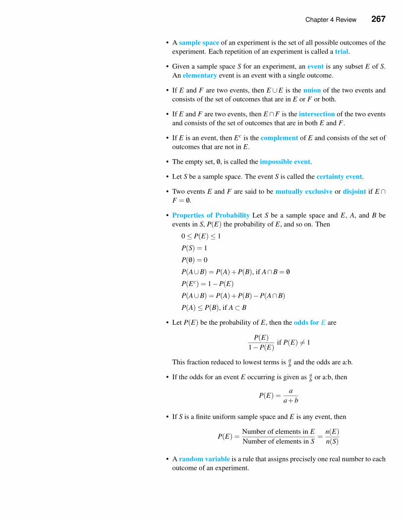
Chapter 4 Review 267
• A sample space of an experiment is the set of all possible outcomes of the
experiment. Each repetition of an experiment is called a trial.
• Given a sample space S for an experiment, an event is any subset E of S.
An elementary event is an event with a single outcome.
• If E and F are two events, then E ∪E is the union of the two events and
consists of the set of outcomes that are in E or F or both.
• If E and F are two events, then E ∩F is the intersection of the two events
and consists of the set of outcomes that are in both E and F .
• If E is an event, then Ec is the complement of E and consists of the set of
outcomes that are not in E.
• The empty set, /0, is called the impossible event.
• Let S be a sample space. The event S is called the certainty event.
• Two events E and F are said to be mutually exclusive or disjoint if E ∩F = /0.
• Properties of Probability Let S be a sample space and E, A, and B be
events in S, P(E) the probability of E, and so on. Then
0≤ P(E)≤ 1
P(S) = 1
P( /0) = 0
P(A∪B) = P(A)+P(B), if A∩B = /0
P(Ec) = 1−P(E)
P(A∪B) = P(A)+P(B)−P(A∩B)
P(A)≤ P(B), if A⊂ B
• Let P(E) be the probability of E, then the odds for E are
P(E)
1−P(E)if P(E) 6= 1
This fraction reduced to lowest terms is ab
and the odds are a:b.
• If the odds for an event E occurring is given as ab
or a:b, then
P(E) =a
a+b
• If S is a finite uniform sample space and E is any event, then
P(E) =Number of elements in E
Number of elements in S=
n(E)
n(S)
• A random variable is a rule that assigns precisely one real number to each
outcome of an experiment.
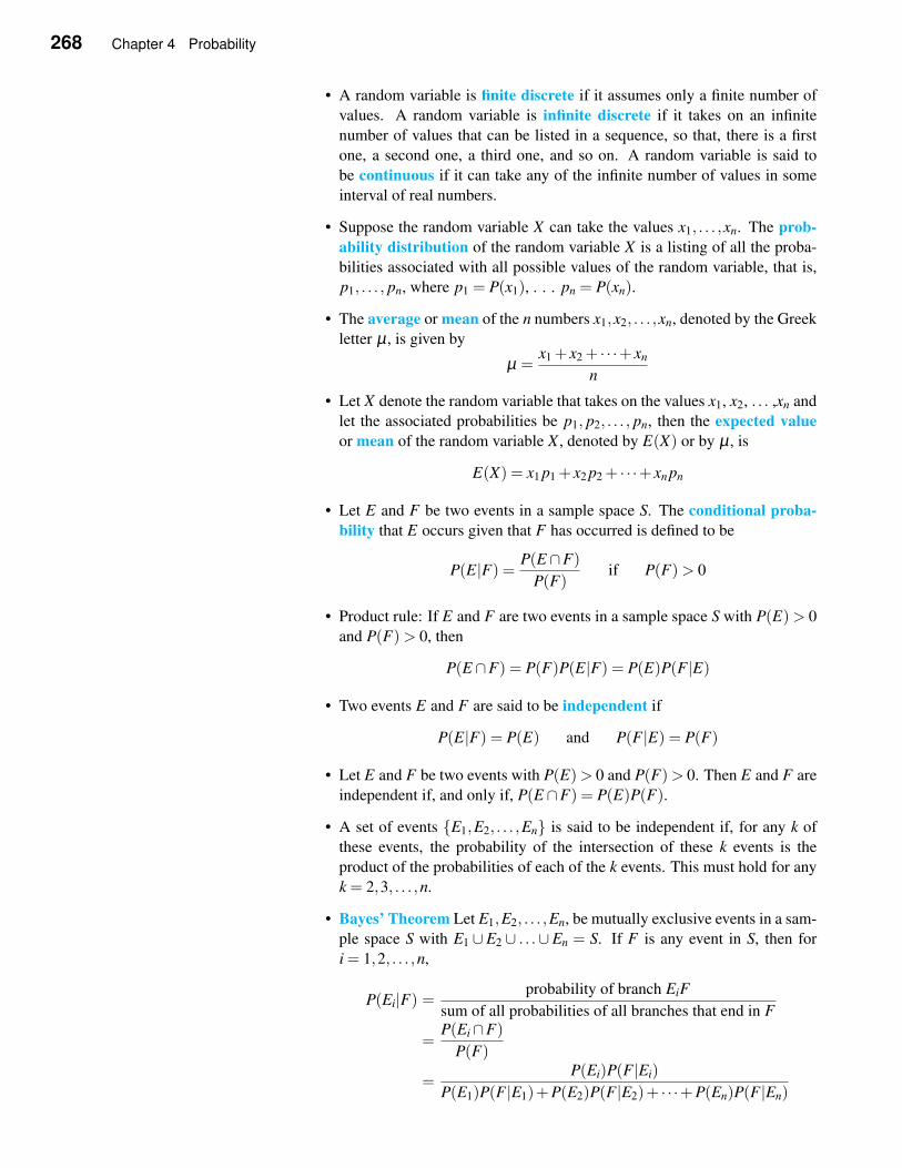
268 Chapter 4 Probability
• A random variable is finite discrete if it assumes only a finite number of
values. A random variable is infinite discrete if it takes on an infinite
number of values that can be listed in a sequence, so that, there is a first
one, a second one, a third one, and so on. A random variable is said to
be continuous if it can take any of the infinite number of values in some
interval of real numbers.
• Suppose the random variable X can take the values x1, . . . ,xn. The prob-
ability distribution of the random variable X is a listing of all the proba-
bilities associated with all possible values of the random variable, that is,
p1, . . . , pn, where p1 = P(x1), . . . pn = P(xn).
• The average or mean of the n numbers x1,x2, . . . ,xn, denoted by the Greek
letter µ , is given by
µ =x1 + x2 + · · ·+ xn
n
• Let X denote the random variable that takes on the values x1, x2, . . . ,xn and
let the associated probabilities be p1, p2, . . . , pn, then the expected value
or mean of the random variable X , denoted by E(X) or by µ , is
E(X) = x1 p1 + x2 p2 + · · ·+ xn pn
• Let E and F be two events in a sample space S. The conditional proba-
bility that E occurs given that F has occurred is defined to be
P(E|F) =P(E ∩F)
P(F)if P(F)> 0
• Product rule: If E and F are two events in a sample space S with P(E)> 0
and P(F)> 0, then
P(E ∩F) = P(F)P(E|F) = P(E)P(F|E)
• Two events E and F are said to be independent if
P(E|F) = P(E) and P(F|E) = P(F)
• Let E and F be two events with P(E)> 0 and P(F)> 0. Then E and F are
independent if, and only if, P(E ∩F) = P(E)P(F).
• A set of events {E1,E2, . . . ,En} is said to be independent if, for any k of
these events, the probability of the intersection of these k events is the
product of the probabilities of each of the k events. This must hold for any
k = 2,3, . . . ,n.
• Bayes’ Theorem Let E1,E2, . . . ,En, be mutually exclusive events in a sam-
ple space S with E1 ∪E2 ∪ . . .∪En = S. If F is any event in S, then for
i = 1,2, . . . ,n,
P(Ei|F) =probability of branch EiF
sum of all probabilities of all branches that end in F
=P(Ei∩F)
P(F)
=P(Ei)P(F|Ei)
P(E1)P(F|E1)+P(E2)P(F|E2)+ · · ·+P(En)P(F|En)
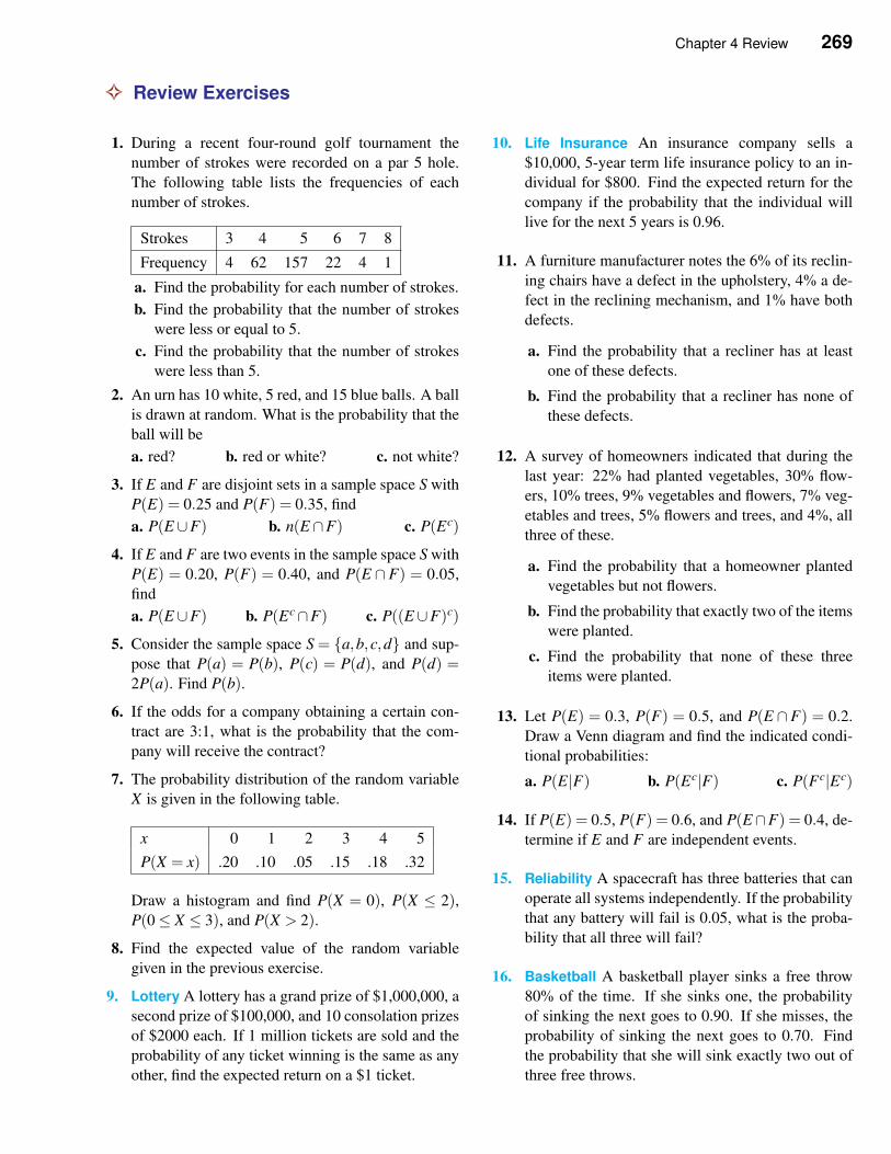
Chapter 4 Review 269
✧ Review Exercises
1. During a recent four-round golf tournament the
number of strokes were recorded on a par 5 hole.
The following table lists the frequencies of each
number of strokes.
Strokes 3 4 5 6 7 8
Frequency 4 62 157 22 4 1
a. Find the probability for each number of strokes.
b. Find the probability that the number of strokes
were less or equal to 5.
c. Find the probability that the number of strokes
were less than 5.
2. An urn has 10 white, 5 red, and 15 blue balls. A ball
is drawn at random. What is the probability that the
ball will be
a. red? b. red or white? c. not white?
3. If E and F are disjoint sets in a sample space S with
P(E) = 0.25 and P(F) = 0.35, find
a. P(E ∪F) b. n(E ∩F) c. P(Ec)
4. If E and F are two events in the sample space S with
P(E) = 0.20, P(F) = 0.40, and P(E ∩F) = 0.05,
find
a. P(E ∪F) b. P(Ec∩F) c. P((E ∪F)c)
5. Consider the sample space S = {a,b,c,d} and sup-
pose that P(a) = P(b), P(c) = P(d), and P(d) =2P(a). Find P(b).
6. If the odds for a company obtaining a certain con-
tract are 3:1, what is the probability that the com-
pany will receive the contract?
7. The probability distribution of the random variable
X is given in the following table.
x 0 1 2 3 4 5
P(X = x) .20 .10 .05 .15 .18 .32
Draw a histogram and find P(X = 0), P(X ≤ 2),P(0≤ X ≤ 3), and P(X > 2).
8. Find the expected value of the random variable
given in the previous exercise.
9. Lottery A lottery has a grand prize of $1,000,000, a
second prize of $100,000, and 10 consolation prizes
of $2000 each. If 1 million tickets are sold and the
probability of any ticket winning is the same as any
other, find the expected return on a $1 ticket.
10. Life Insurance An insurance company sells a
$10,000, 5-year term life insurance policy to an in-
dividual for $800. Find the expected return for the
company if the probability that the individual will
live for the next 5 years is 0.96.
11. A furniture manufacturer notes the 6% of its reclin-
ing chairs have a defect in the upholstery, 4% a de-
fect in the reclining mechanism, and 1% have both
defects.
a. Find the probability that a recliner has at least
one of these defects.
b. Find the probability that a recliner has none of
these defects.
12. A survey of homeowners indicated that during the
last year: 22% had planted vegetables, 30% flow-
ers, 10% trees, 9% vegetables and flowers, 7% veg-
etables and trees, 5% flowers and trees, and 4%, all
three of these.
a. Find the probability that a homeowner planted
vegetables but not flowers.
b. Find the probability that exactly two of the items
were planted.
c. Find the probability that none of these three
items were planted.
13. Let P(E) = 0.3, P(F) = 0.5, and P(E ∩F) = 0.2.
Draw a Venn diagram and find the indicated condi-
tional probabilities:
a. P(E|F) b. P(Ec|F) c. P(Fc|Ec)
14. If P(E) = 0.5, P(F) = 0.6, and P(E ∩F) = 0.4, de-
termine if E and F are independent events.
15. Reliability A spacecraft has three batteries that can
operate all systems independently. If the probability
that any battery will fail is 0.05, what is the proba-
bility that all three will fail?
16. Basketball A basketball player sinks a free throw
80% of the time. If she sinks one, the probability
of sinking the next goes to 0.90. If she misses, the
probability of sinking the next goes to 0.70. Find
the probability that she will sink exactly two out of
three free throws.
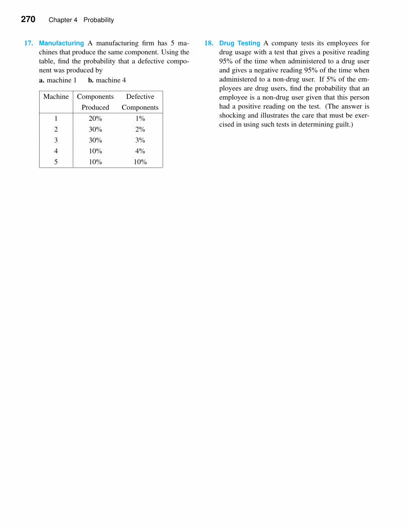
270 Chapter 4 Probability
17. Manufacturing A manufacturing firm has 5 ma-
chines that produce the same component. Using the
table, find the probability that a defective compo-
nent was produced by
a. machine 1 b. machine 4
Machine Components Defective
Produced Components
1 20% 1%
2 30% 2%
3 30% 3%
4 10% 4%
5 10% 10%
18. Drug Testing A company tests its employees for
drug usage with a test that gives a positive reading
95% of the time when administered to a drug user
and gives a negative reading 95% of the time when
administered to a non-drug user. If 5% of the em-
ployees are drug users, find the probability that an
employee is a non-drug user given that this person
had a positive reading on the test. (The answer is
shocking and illustrates the care that must be exer-
cised in using such tests in determining guilt.)
CHAPTER 5Functions and Models
Quadratic model of revenue are more realistic
than the linear models discussed in Chapter 1.
A linear model assumes that the price per items
stays the same. So if a buyer purchases one
widget or one million widgets, the price each
stays the same. Along those same lines, in a lin-
ear revenue model, the revenue can be infinitely
large - clearly unrealistic.
In a quadratic model, we assume the price (de-
mand) is a linear function, p = D(x) = mx+b.
That will give us a quadratic revenue function,
R(x) = xp = x(mx+b). In this chapter we will
learn how to find where the revenue is maxi-
mized. One example we will study is the rev-
enue for recycling. If the price for a household
to recycle is not too high, the revenue can be
increased to a point by increasing the price per
household. However, if the price becomes too
high, the demand for recycling will drop and
the revenue will also drop. See page 278.
5.1 Polynomials
APPLICATION
Mathematical Modeling
From all four corners of a 10-inch by 20-inch rectangular piece of card-
board, squares are cut with dimensions x by x. The sides of the remaining
piece of cardboard are turned up to form an open box. Find a formula that
gives the volume V of the box in terms of x. See Example 11 on page 280
for the answer.
Recall from Chapter 1 the definition of a function.
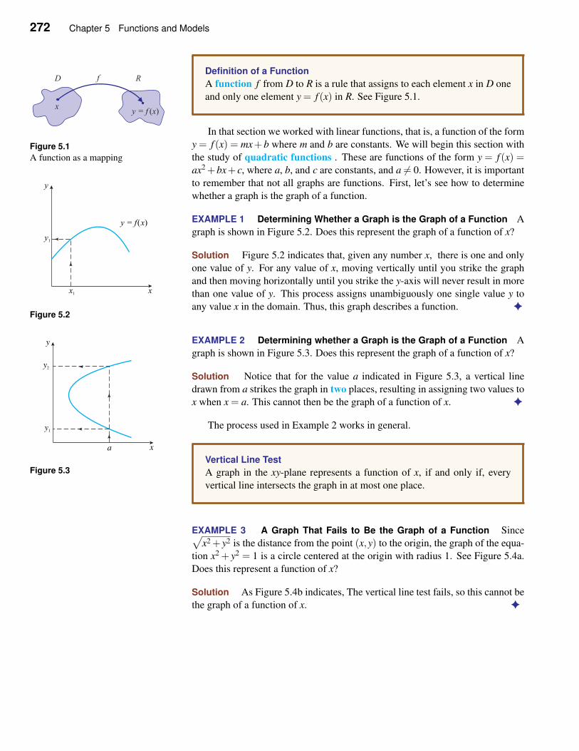
272 Chapter 5 Functions and Models
Definition of a Function
A function f from D to R is a rule that assigns to each element x in D one
and only one element y = f (x) in R. See Figure 5.1.
Figure 5.1
A function as a mapping
In that section we worked with linear functions, that is, a function of the form
y = f (x) = mx+b where m and b are constants. We will begin this section with
the study of quadratic functions . These are functions of the form y = f (x) =ax2 +bx+ c, where a, b, and c are constants, and a 6= 0. However, it is important
to remember that not all graphs are functions. First, let’s see how to determine
whether a graph is the graph of a function.
EXAMPLE 1 Determining Whether a Graph is the Graph of a Function A
graph is shown in Figure 5.2. Does this represent the graph of a function of x?
Solution Figure 5.2 indicates that, given any number x, there is one and only
xx1
y
y1
y = f x( )
Figure 5.2
one value of y. For any value of x, moving vertically until you strike the graph
and then moving horizontally until you strike the y-axis will never result in more
than one value of y. This process assigns unambiguously one single value y to
any value x in the domain. Thus, this graph describes a function. ✦
EXAMPLE 2 Determining whether a Graph is the Graph of a Function A
graph is shown in Figure 5.3. Does this represent the graph of a function of x?
Solution Notice that for the value a indicated in Figure 5.3, a vertical line
drawn from a strikes the graph in two places, resulting in assigning two values to
x when x = a. This cannot then be the graph of a function of x. ✦
x
y
y1
y2
a
Figure 5.3
The process used in Example 2 works in general.
Vertical Line Test
A graph in the xy-plane represents a function of x, if and only if, every
vertical line intersects the graph in at most one place.
EXAMPLE 3 A Graph That Fails to Be the Graph of a Function Since√
x2 + y2 is the distance from the point (x,y) to the origin, the graph of the equa-
tion x2 + y2 = 1 is a circle centered at the origin with radius 1. See Figure 5.4a.
Does this represent a function of x?
Solution As Figure 5.4b indicates, The vertical line test fails, so this cannot be
the graph of a function of x. ✦
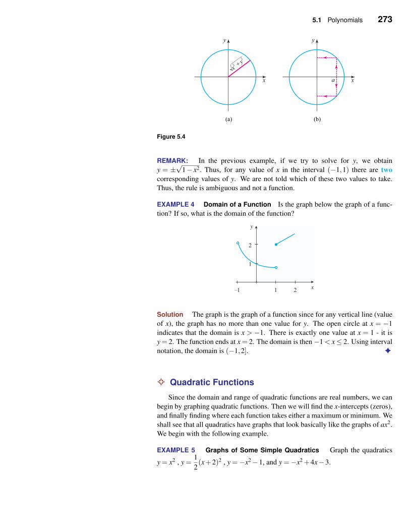
5.1 Polynomials 273
x
y
x
y
√x2 + y
2
a
(b)(a)
Figure 5.4
REMARK: In the previous example, if we try to solve for y, we obtain
y = ±√
1− x2. Thus, for any value of x in the interval (−1,1) there are two
corresponding values of y. We are not told which of these two values to take.
Thus, the rule is ambiguous and not a function.
EXAMPLE 4 Domain of a Function Is the graph below the graph of a func-
tion? If so, what is the domain of the function?
y
x1 2
1
2
-1
Solution The graph is the graph of a function since for any vertical line (value
of x), the graph has no more than one value for y. The open circle at x = −1
indicates that the domain is x > −1. There is exactly one value at x = 1 - it is
y = 2. The function ends at x = 2. The domain is then−1 < x≤ 2. Using interval
notation, the domain is (−1,2]. ✦
✧ Quadratic Functions
Since the domain and range of quadratic functions are real numbers, we can
begin by graphing quadratic functions. Then we will find the x-intercepts (zeros),
and finally finding where each function takes either a maximum or minimum. We
shall see that all quadratics have graphs that look basically like the graphs of ax2.
We begin with the following example.
EXAMPLE 5 Graphs of Some Simple Quadratics Graph the quadratics
y = x2 , y =1
2(x+2)2 , y =−x2−1, and y =−x2 +4x−3.
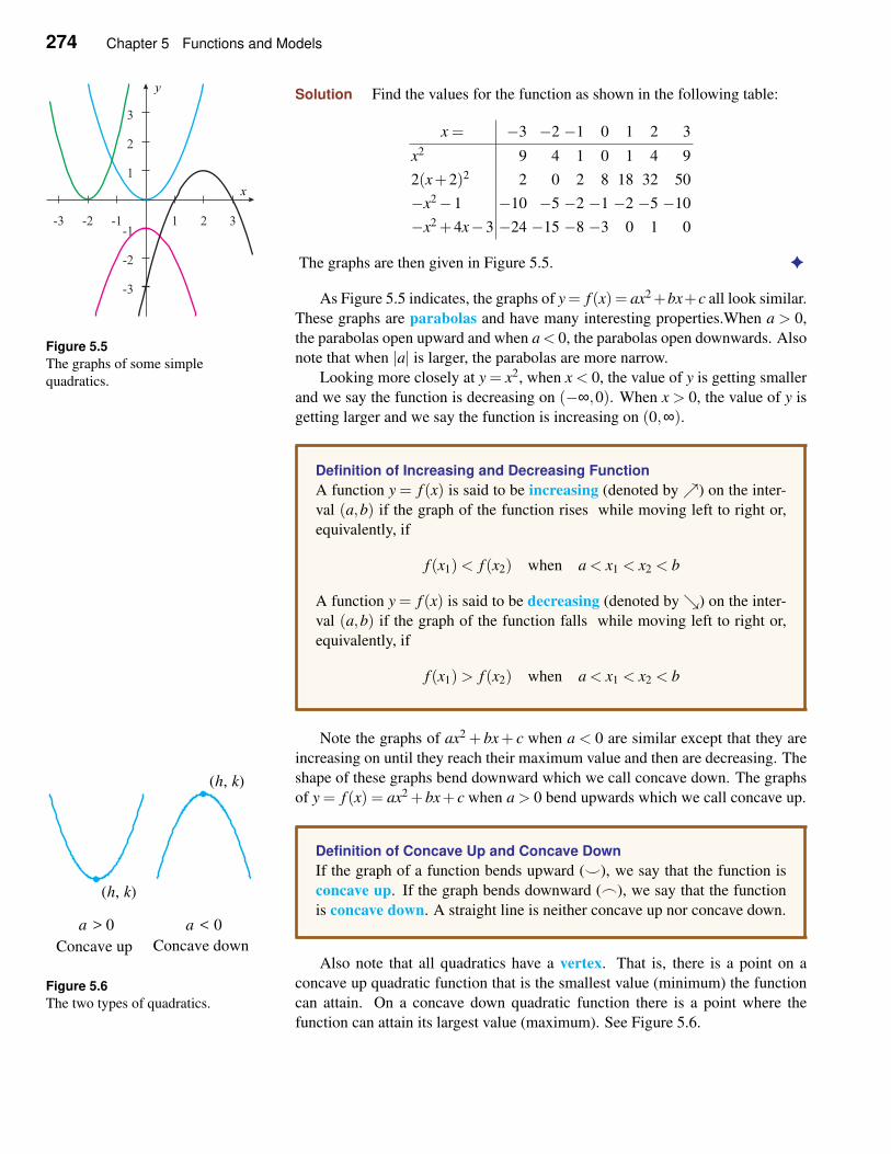
274 Chapter 5 Functions and Models
Solution Find the values for the function as shown in the following table:
x = −3 −2 −1 0 1 2 3
x2 9 4 1 0 1 4 9
2(x+2)2 2 0 2 8 18 32 50
−x2−1 −10 −5 −2 −1 −2 −5 −10
−x2 +4x−3 −24 −15 −8 −3 0 1 0
The graphs are then given in Figure 5.5. ✦
-3 -2 -1 1 2 3
-3
-2
-1
1
2
3
x
y
Figure 5.5
The graphs of some simple
quadratics.
As Figure 5.5 indicates, the graphs of y= f (x) = ax2+bx+c all look similar.
These graphs are parabolas and have many interesting properties.When a > 0,
the parabolas open upward and when a < 0, the parabolas open downwards. Also
note that when |a| is larger, the parabolas are more narrow.
Looking more closely at y = x2, when x < 0, the value of y is getting smaller
and we say the function is decreasing on (−∞,0). When x > 0, the value of y is
getting larger and we say the function is increasing on (0,∞).
Definition of Increasing and Decreasing Function
A function y = f (x) is said to be increasing (denoted byր) on the inter-
val (a,b) if the graph of the function rises while moving left to right or,
equivalently, if
f (x1)< f (x2) when a < x1 < x2 < b
A function y = f (x) is said to be decreasing (denoted byց) on the inter-
val (a,b) if the graph of the function falls while moving left to right or,
equivalently, if
f (x1)> f (x2) when a < x1 < x2 < b
Note the graphs of ax2 + bx+ c when a < 0 are similar except that they are
increasing on until they reach their maximum value and then are decreasing. The
shape of these graphs bend downward which we call concave down. The graphs
of y = f (x) = ax2 +bx+ c when a > 0 bend upwards which we call concave up.
Definition of Concave Up and Concave Down
If the graph of a function bends upward (⌣), we say that the function is
concave up. If the graph bends downward (⌢), we say that the function
is concave down. A straight line is neither concave up nor concave down.
(h, k)
(h, k)
a > 0 a < 0
Concave up Concave down
Figure 5.6
The two types of quadratics.
Also note that all quadratics have a vertex. That is, there is a point on a
concave up quadratic function that is the smallest value (minimum) the function
can attain. On a concave down quadratic function there is a point where the
function can attain its largest value (maximum). See Figure 5.6.
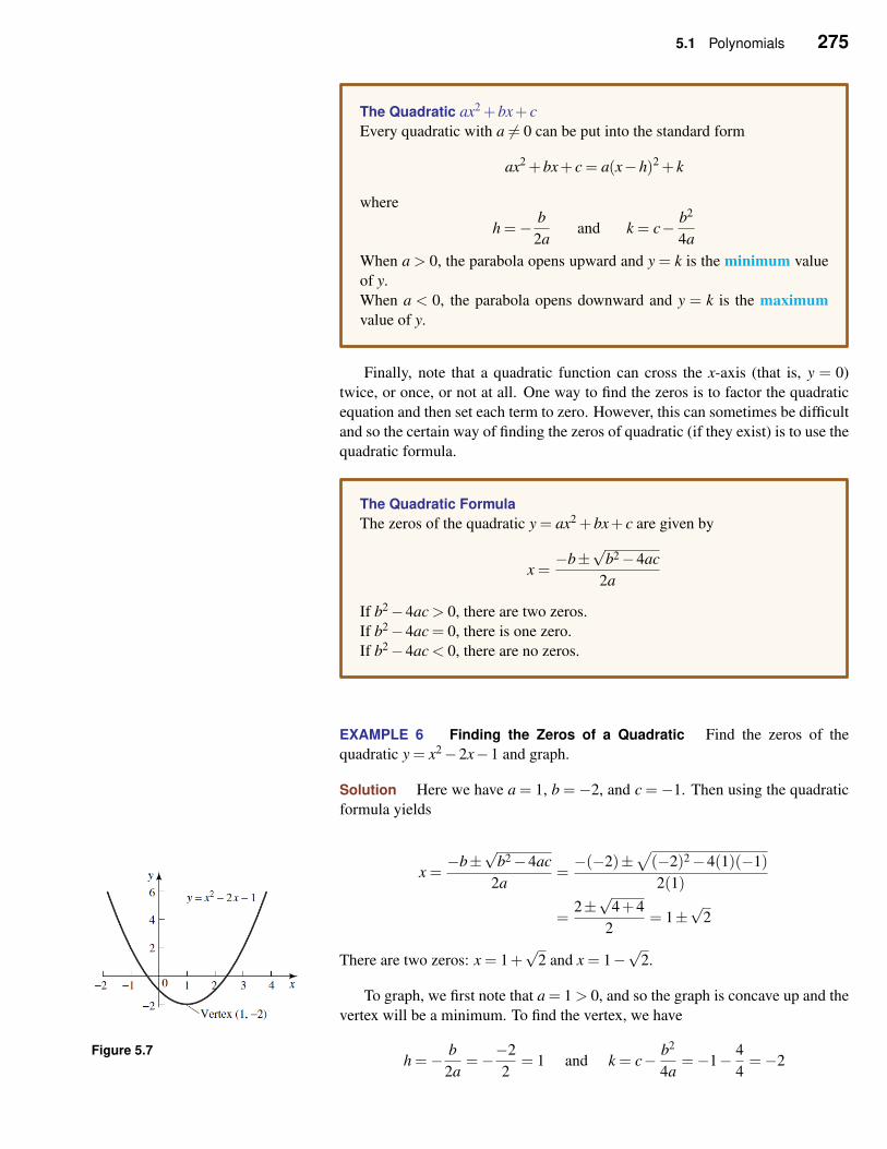
5.1 Polynomials 275
The Quadratic ax2 +bx+ c
Every quadratic with a 6= 0 can be put into the standard form
ax2 +bx+ c = a(x−h)2 + k
where
h =− b
2aand k = c− b2
4a
When a > 0, the parabola opens upward and y = k is the minimum value
of y.
When a < 0, the parabola opens downward and y = k is the maximum
value of y.
Finally, note that a quadratic function can cross the x-axis (that is, y = 0)
twice, or once, or not at all. One way to find the zeros is to factor the quadratic
equation and then set each term to zero. However, this can sometimes be difficult
and so the certain way of finding the zeros of quadratic (if they exist) is to use the
quadratic formula.
The Quadratic Formula
The zeros of the quadratic y = ax2 +bx+ c are given by
x =−b±
√b2−4ac
2a
If b2−4ac > 0, there are two zeros.
If b2−4ac = 0, there is one zero.
If b2−4ac < 0, there are no zeros.
EXAMPLE 6 Finding the Zeros of a Quadratic Find the zeros of the
quadratic y = x2−2x−1 and graph.
Solution Here we have a = 1, b =−2, and c =−1. Then using the quadratic
formula yields
x =−b±
√b2−4ac
2a=−(−2)±
√
(−2)2−4(1)(−1)
2(1)
=2±√
4+4
2= 1±
√2
There are two zeros: x = 1+√
2 and x = 1−√
2.
To graph, we first note that a = 1 > 0, and so the graph is concave up and the
vertex will be a minimum. To find the vertex, we have
Figure 5.7h =− b
2a=−−2
2= 1 and k = c− b2
4a=−1− 4
4=−2
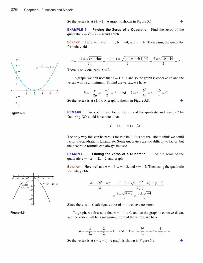
276 Chapter 5 Functions and Models
So the vertex is at (1,−2). A graph is shown in Figure 5.7. ✦
EXAMPLE 7 Finding the Zeros of a Quadratic Find the zeros of the
quadratic y = x2−4x+4 and graph.
Solution Here we have a = 1, b = −4, and c = 4. Then using the quadratic
formula yields
x =−b±
√b2−4ac
2a=−(−4)±
√
(−4)2−4(1)(4)
2=
4±√
16−16
2= 2
There is only one zero: x = 2.
To graph, we first note that a = 1 > 0, and so the graph is concave up and the
vertex will be a minimum. To find the vertex, we have
h =− b
2a=−−4
2= 2 and k = c− b2
4a= 4− 16
4= 0
So the vertex is at (2,0). A graph is shown in Figure 5.8. ✦
1 2 3 4
-4
-2
2
4
6
8
y
x
y x x= 4 + 42-
Figure 5.8 REMARK: We could have found the zero of the quadratic in Example7 by
factoring. We could have noted that
x2−4x+4 = (x−2)2
The only way this can be zero is for x to be 2. It is not realistic to think we could
factor the quadratic in Example6. Some quadratics are too difficult to factor, but
the quadratic formula can always be used.
EXAMPLE 8 Finding the Zeros of a Quadratic Find the zeros of the
quadratic y =−x2−2x−2, and graph.
Solution Here we have a =−1, b =−2, and c =−2. Then using the quadratic
formula yields
−b±√
b2−4ac
2a=−(−2)±
√
(−2)2−4(−1)(−2)
2(1)
=2±√
4−8
2=
2±√−4
2
Since there is no (real) square root of −4, we have no zeros.
Figure 5.9 To graph, we first note that a = −1 < 0, and so the graph is concave down,
and the vertex will be a maximum. To find the vertex, we have
h =− b
2a=−−2
−2=−1 and k = c− b2
4a=−2− 4
−4=−1
So the vertex is at (−1,−1). A graph is shown in Figure 5.9. ✦
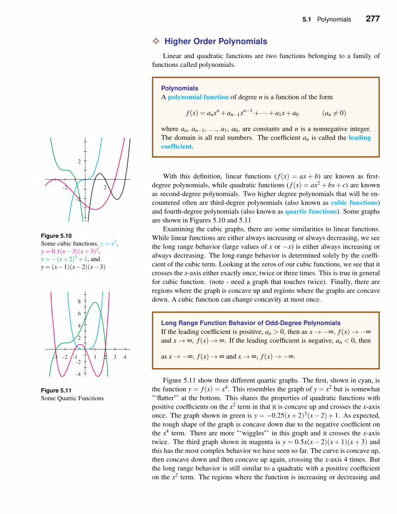
5.1 Polynomials 277
✧ Higher Order Polynomials
Linear and quadratic functions are two functions belonging to a family of
functions called polynomials.
Polynomials
A polynomial function of degree n is a function of the form
f (x) = anxn +an−1xn−1 + · · ·+a1x+a0 (an 6= 0)
where an, an−1, . . ., a1, a0, are constants and n is a nonnegative integer.
The domain is all real numbers. The coefficient an is called the leading
coefficient.
With this definition, linear functions ( f (x) = ax + b) are known as first-
degree polynomials, while quadratic functions ( f (x) = ax2 + bx+ c) are known
as second-degree polynomials. Two higher degree polynomials that will be en-
countered often are third-degree polynomials (also known as cubic functions)
and fourth-degree polynomials (also known as quartic functions). Some graphs
are shown in Figures 5.10 and 5.11
-2 2
-2
2
Figure 5.10
Some cubic functions, y = x3,
y = 0.1(x−3)(x+3)2,
y =−(x+2)3 +1, and
y = (x−1)(x−2)(x−3)
Examining the cubic graphs, there are some similarities to linear functions.
While linear functions are either always increasing or always decreasing, we see
the long range behavior (large values of x or −x) is either always increasing or
always decreasing. The long-range behavior is determined solely by the coeffi-
cient of the cubic term. Looking at the zeros of our cubic functions, we see that it
crosses the x-axis either exactly once, twice or three times. This is true in general
for cubic function. (note - need a graph that touches twice). Finally, there are
regions where the graph is concave up and regions where the graphs are concave
down. A cubic function can change concavity at most once.
Long Range Function Behavior of Odd-Degree Polynomials
If the leading coefficient is positive, an > 0, then as x→−∞, f (x)→−∞and x→ ∞, f (x)→ ∞. If the leading coefficient is negative, an < 0, then
as x→−∞, f (x)→ ∞ and x→ ∞, f (x)→−∞.-3 -2 -1 1 2 3 4
-4
-2
2
4
6
8
Figure 5.11
Some Quartic Functions
Figure 5.11 show three different quartic graphs. The first, shown in cyan, is
the function y = f (x) = x4. This resembles the graph of y = x2 but is somewhat
"‘flatter"’ at the bottom. This shares the properties of quadratic functions with
positive coefficients on the x2 term in that it is concave up and crosses the x-axis
once. The graph shown in green is y = −0.25(x+ 2)3(x− 2)+ 1. As expected,
the rough shape of the graph is concave down due to the negative coefficient on
the x4 term. There are more "‘wiggles"’ in this graph and it crosses the x-axis
twice. The third graph shown in magenta is y = 0.5x(x− 2)(x+ 1)(x+ 3) and
this has the most complex behavior we have seen so far. The curve is concave up,
then concave down and then concave up again, crossing the x-axis 4 times. But
the long range behavior is still similar to a quadratic with a positive coefficient
on the x2 term. The regions where the function is increasing or decreasing and
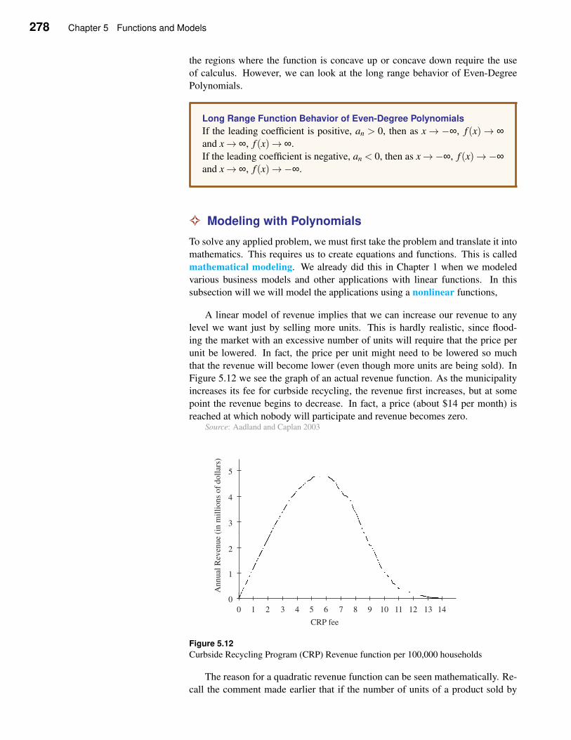
278 Chapter 5 Functions and Models
the regions where the function is concave up or concave down require the use
of calculus. However, we can look at the long range behavior of Even-Degree
Polynomials.
Long Range Function Behavior of Even-Degree Polynomials
If the leading coefficient is positive, an > 0, then as x→−∞, f (x)→ ∞and x→ ∞, f (x)→ ∞.
If the leading coefficient is negative, an < 0, then as x→−∞, f (x)→−∞and x→ ∞, f (x)→−∞.
✧ Modeling with Polynomials
To solve any applied problem, we must first take the problem and translate it into
mathematics. This requires us to create equations and functions. This is called
mathematical modeling. We already did this in Chapter 1 when we modeled
various business models and other applications with linear functions. In this
subsection will we will model the applications using a nonlinear functions,
A linear model of revenue implies that we can increase our revenue to any
level we want just by selling more units. This is hardly realistic, since flood-
ing the market with an excessive number of units will require that the price per
unit be lowered. In fact, the price per unit might need to be lowered so much
that the revenue will become lower (even though more units are being sold). In
Figure 5.12 we see the graph of an actual revenue function. As the municipality
increases its fee for curbside recycling, the revenue first increases, but at some
point the revenue begins to decrease. In fact, a price (about $14 per month) is
reached at which nobody will participate and revenue becomes zero.Source: Aadland and Caplan 2003
0 1 2 3 4 5 6 7 8 9 10 11 12 13 14
0
1
2
3
4
5
CRP fee
Annual
Rev
enue
(in m
illi
ons
of
doll
ars)
Figure 5.12
Curbside Recycling Program (CRP) Revenue function per 100,000 households
The reason for a quadratic revenue function can be seen mathematically. Re-
call the comment made earlier that if the number of units of a product sold by
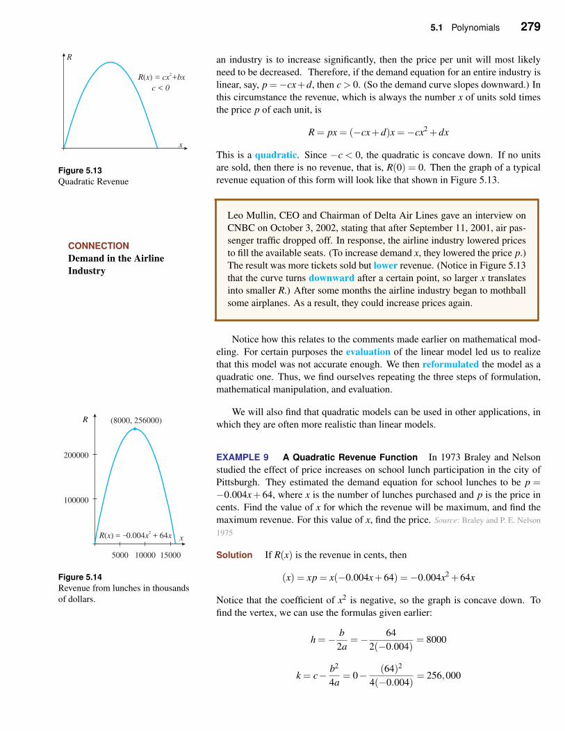
5.1 Polynomials 279
an industry is to increase significantly, then the price per unit will most likely
need to be decreased. Therefore, if the demand equation for an entire industry isR x = cx +bx( )
2
c < 0
R
x
Figure 5.13
Quadratic Revenue
linear, say, p =−cx+d, then c > 0. (So the demand curve slopes downward.) In
this circumstance the revenue, which is always the number x of units sold times
the price p of each unit, is
R = px = (−cx+d)x =−cx2 +dx
This is a quadratic. Since −c < 0, the quadratic is concave down. If no units
are sold, then there is no revenue, that is, R(0) = 0. Then the graph of a typical
revenue equation of this form will look like that shown in Figure 5.13.
CONNECTION
Demand in the Airline
Industry
Leo Mullin, CEO and Chairman of Delta Air Lines gave an interview on
CNBC on October 3, 2002, stating that after September 11, 2001, air pas-
senger traffic dropped off. In response, the airline industry lowered prices
to fill the available seats. (To increase demand x, they lowered the price p.)
The result was more tickets sold but lower revenue. (Notice in Figure 5.13
that the curve turns downward after a certain point, so larger x translates
into smaller R.) After some months the airline industry began to mothball
some airplanes. As a result, they could increase prices again.
Notice how this relates to the comments made earlier on mathematical mod-
eling. For certain purposes the evaluation of the linear model led us to realize
that this model was not accurate enough. We then reformulated the model as a
quadratic one. Thus, we find ourselves repeating the three steps of formulation,
mathematical manipulation, and evaluation.
We will also find that quadratic models can be used in other applications, in
which they are often more realistic than linear models.
EXAMPLE 9 A Quadratic Revenue Function In 1973 Braley and Nelson
studied the effect of price increases on school lunch participation in the city of
Pittsburgh. They estimated the demand equation for school lunches to be p =−0.004x+ 64, where x is the number of lunches purchased and p is the price in
cents. Find the value of x for which the revenue will be maximum, and find the
maximum revenue. For this value of x, find the price. Source: Braley and P. E. Nelson
1975
Solution If R(x) is the revenue in cents, then
R
xR x x x( ) = 0.004 + 64-
2
(8000, 256000)
5000 10000 15000
100000
200000
Figure 5.14
Revenue from lunches in thousands
of dollars.
(x) = xp = x(−0.004x+64) =−0.004x2 +64x
Notice that the coefficient of x2 is negative, so the graph is concave down. To
find the vertex, we can use the formulas given earlier:
h =− b
2a=− 64
2(−0.004)= 8000
k = c− b2
4a= 0− (64)2
4(−0.004)= 256,000
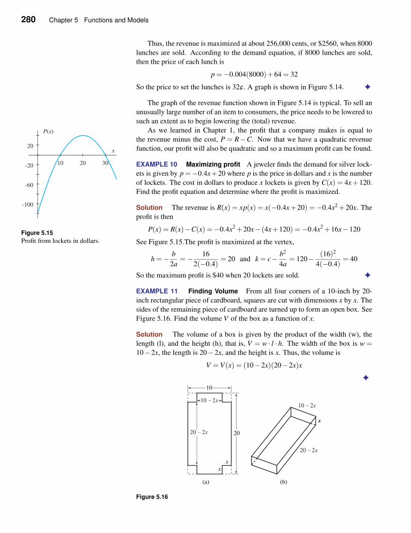
280 Chapter 5 Functions and Models
Thus, the revenue is maximized at about 256,000 cents, or $2560, when 8000
lunches are sold. According to the demand equation, if 8000 lunches are sold,
then the price of each lunch is
p =−0.004(8000)+64 = 32
So the price to set the lunches is 32¢. A graph is shown in Figure 5.14. ✦
The graph of the revenue function shown in Figure 5.14 is typical. To sell an
unusually large number of an item to consumers, the price needs to be lowered to
such an extent as to begin lowering the (total) revenue.
As we learned in Chapter 1, the profit that a company makes is equal to
the revenue minus the cost, P = R−C. Now that we have a quadratic revenue
function, our profit will also be quadratic and so a maximum profit can be found.
EXAMPLE 10 Maximizing profit A jeweler finds the demand for silver lock-
ets is given by p =−0.4x+20 where p is the price in dollars and x is the number
of lockets. The cost in dollars to produce x lockets is given by C(x) = 4x+120.
Find the profit equation and determine where the profit is maximized.
Solution The revenue is R(x) = xp(x) = x(−0.4x+20) =−0.4x2 +20x. The
profit is then
10 20 30
-100
-60
-20
20x
P x( )
Figure 5.15
Profit from lockets in dollars.
P(x) = R(x)−C(x) =−0.4x2 +20x− (4x+120) =−0.4x2 +16x−120
See Figure 5.15.The profit is maximized at the vertex,
h =− b
2a=− 16
2(−0.4)= 20 and k = c− b2
4a= 120− (16)2
4(−0.4)= 40
So the maximum profit is $40 when 20 lockets are sold. ✦
EXAMPLE 11 Finding Volume From all four corners of a 10-inch by 20-
inch rectangular piece of cardboard, squares are cut with dimensions x by x. The
sides of the remaining piece of cardboard are turned up to form an open box. See
Figure 5.16. Find the volume V of the box as a function of x.
Solution The volume of a box is given by the product of the width (w), the
length (l), and the height (h), that is, V = w · l · h. The width of the box is w =10−2x, the length is 20−2x, and the height is x. Thus, the volume is
V =V (x) = (10−2x)(20−2x)x
✦
20
10
x
x
(a) (b)
x
10 2- x10 2- x
20 2- x
20 2- x
Figure 5.16
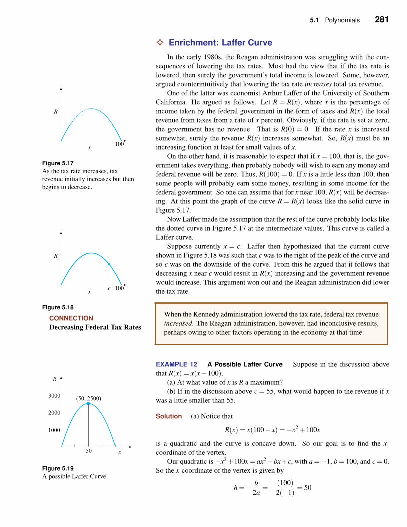
5.1 Polynomials 281
✧ Enrichment: Laffer Curve
In the early 1980s, the Reagan administration was struggling with the con-
sequences of lowering the tax rates. Most had the view that if the tax rate is
lowered, then surely the government’s total income is lowered. Some, however,
argued counterintuitively that lowering the tax rate increases total tax revenue.
One of the latter was economist Arthur Laffer of the University of Southern
California. He argued as follows. Let R = R(x), where x is the percentage of
income taken by the federal government in the form of taxes and R(x) the total
revenue from taxes from a rate of x percent. Obviously, if the rate is set at zero,
the government has no revenue. That is R(0) = 0. If the rate x is increased
somewhat, surely the revenue R(x) increases somewhat. So, R(x) must be an
increasing function at least for small values of x.x
R
�
100
Figure 5.17
As the tax rate increases, tax
revenue initially increases but then
begins to decrease.
On the other hand, it is reasonable to expect that if x = 100, that is, the gov-
ernment takes everything, then probably nobody will wish to earn any money and
federal revenue will be zero. Thus, R(100) = 0. If x is a little less than 100, then
some people will probably earn some money, resulting in some income for the
federal government. So one can assume that for x near 100, R(x) will be decreas-
ing. At this point the graph of the curve R = R(x) looks like the solid curve in
Figure 5.17.
Now Laffer made the assumption that the rest of the curve probably looks like
the dotted curve in Figure 5.17 at the intermediate values. This curve is called a
Laffer curve.
Suppose currently x = c. Laffer then hypothesized that the current curve
shown in Figure 5.18 was such that c was to the right of the peak of the curve and
so c was on the downside of the curve. From this he argued that it follows that
decreasing x near c would result in R(x) increasing and the government revenue
would increase. This argument won out and the Reagan administration did lower
the tax rate.x
R
�
c 100
Figure 5.18
CONNECTION
Decreasing Federal Tax Rates
When the Kennedy administration lowered the tax rate, federal tax revenue
increased. The Reagan administration, however, had inconclusive results,
perhaps owing to other factors operating in the economy at that time.
EXAMPLE 12 A Possible Laffer Curve Suppose in the discussion above
that R(x) = x(x−100).(a) At what value of x is R a maximum?
(b) If in the discussion above c = 55, what would happen to the revenue if x
was a little smaller than 55.
Solution (a) Notice that
R(x) = x(100− x) =−x2 +100x
is a quadratic and the curve is concave down. So our goal is to find the x-
coordinate of the vertex.
2000
3000
x
(50, 2500)
1000
50
R
Figure 5.19
A possible Laffer Curve
Our quadratic is−x2+100x = ax2+bx+c, with a =−1, b = 100, and c = 0.
So the x-coordinate of the vertex is given by
h =− b
2a=− (100)
2(−1)= 50
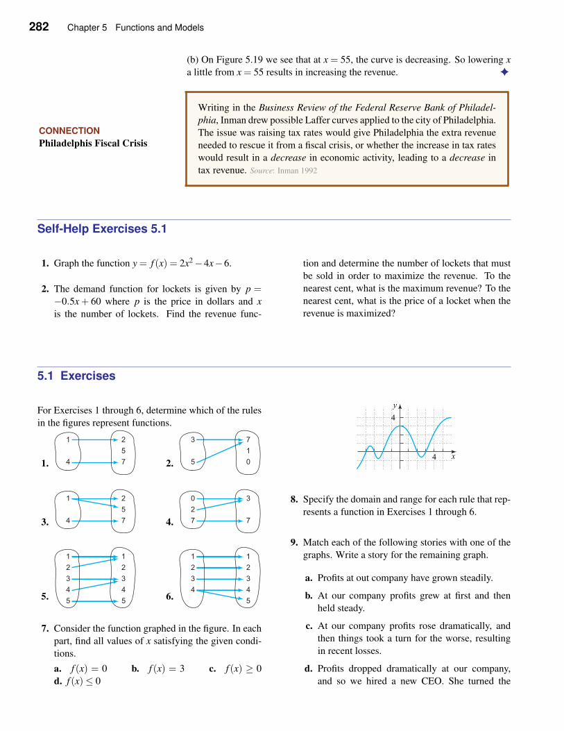
282 Chapter 5 Functions and Models
(b) On Figure 5.19 we see that at x = 55, the curve is decreasing. So lowering x
a little from x = 55 results in increasing the revenue. ✦
CONNECTION
Philadelphis Fiscal Crisis
Writing in the Business Review of the Federal Reserve Bank of Philadel-
phia, Inman drew possible Laffer curves applied to the city of Philadelphia.
The issue was raising tax rates would give Philadelphia the extra revenue
needed to rescue it from a fiscal crisis, or whether the increase in tax rates
would result in a decrease in economic activity, leading to a decrease in
tax revenue. Source: Inman 1992
Self-Help Exercises 5.1
1. Graph the function y = f (x) = 2x2−4x−6.
2. The demand function for lockets is given by p =−0.5x + 60 where p is the price in dollars and x
is the number of lockets. Find the revenue func-
tion and determine the number of lockets that must
be sold in order to maximize the revenue. To the
nearest cent, what is the maximum revenue? To the
nearest cent, what is the price of a locket when the
revenue is maximized?
5.1 Exercises
For Exercises 1 through 6, determine which of the rules
in the figures represent functions.
1. 2.
3. 4.
5. 6.
7. Consider the function graphed in the figure. In each
part, find all values of x satisfying the given condi-
tions.
a. f (x) = 0 b. f (x) = 3 c. f (x) ≥ 0
d. f (x)≤ 0
4 x
y
4
8. Specify the domain and range for each rule that rep-
resents a function in Exercises 1 through 6.
9. Match each of the following stories with one of the
graphs. Write a story for the remaining graph.
a. Profits at out company have grown steadily.
b. At our company profits grew at first and then
held steady.
c. At our company profits rose dramatically, and
then things took a turn for the worse, resulting
in recent losses.
d. Profits dropped dramatically at our company,
and so we hired a new CEO. She turned the
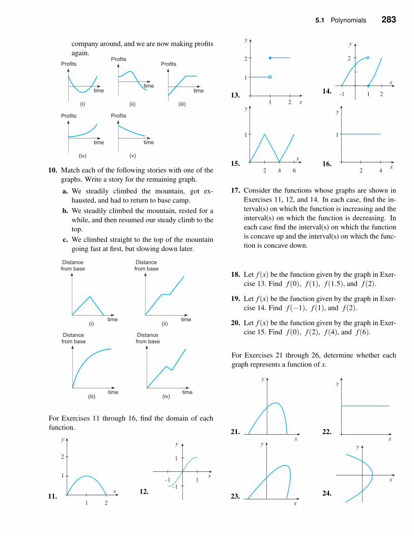
5.1 Polynomials 283
company around, and we are now making profits
again.
10. Match each of the following stories with one of the
graphs. Write a story for the remaining graph.
a. We steadily climbed the mountain, got ex-
hausted, and had to return to base camp.
b. We steadily climbed the mountain, rested for a
while, and then resumed our steady climb to the
top.
c. We climbed straight to the top of the mountain
going fast at first, but slowing down later.
For Exercises 11 through 16, find the domain of each
function.
11.1 2
1
2
y
x 12.
y
x-1 1
-1
1
13.
y
x1 2
1
2
14.
y
x
-1 1 2
2
15.
y
x
2 4 6
1
16.
y
x2 4
1
17. Consider the functions whose graphs are shown in
Exercises 11, 12, and 14. In each case, find the in-
terval(s) on which the function is increasing and the
interval(s) on which the function is decreasing. In
each case find the interval(s) on which the function
is concave up and the interval(s) on which the func-
tion is concave down.
18. Let f (x) be the function given by the graph in Exer-
cise 13. Find f (0), f (1), f (1.5), and f (2).
19. Let f (x) be the function given by the graph in Exer-
cise 14. Find f (−1), f (1), and f (2).
20. Let f (x) be the function given by the graph in Exer-
cise 15. Find f (0), f (2), f (4), and f (6).
For Exercises 21 through 26, determine whether each
graph represents a function of x.
21.
y
x22.
y
x
23.
y
x
24.
y
x
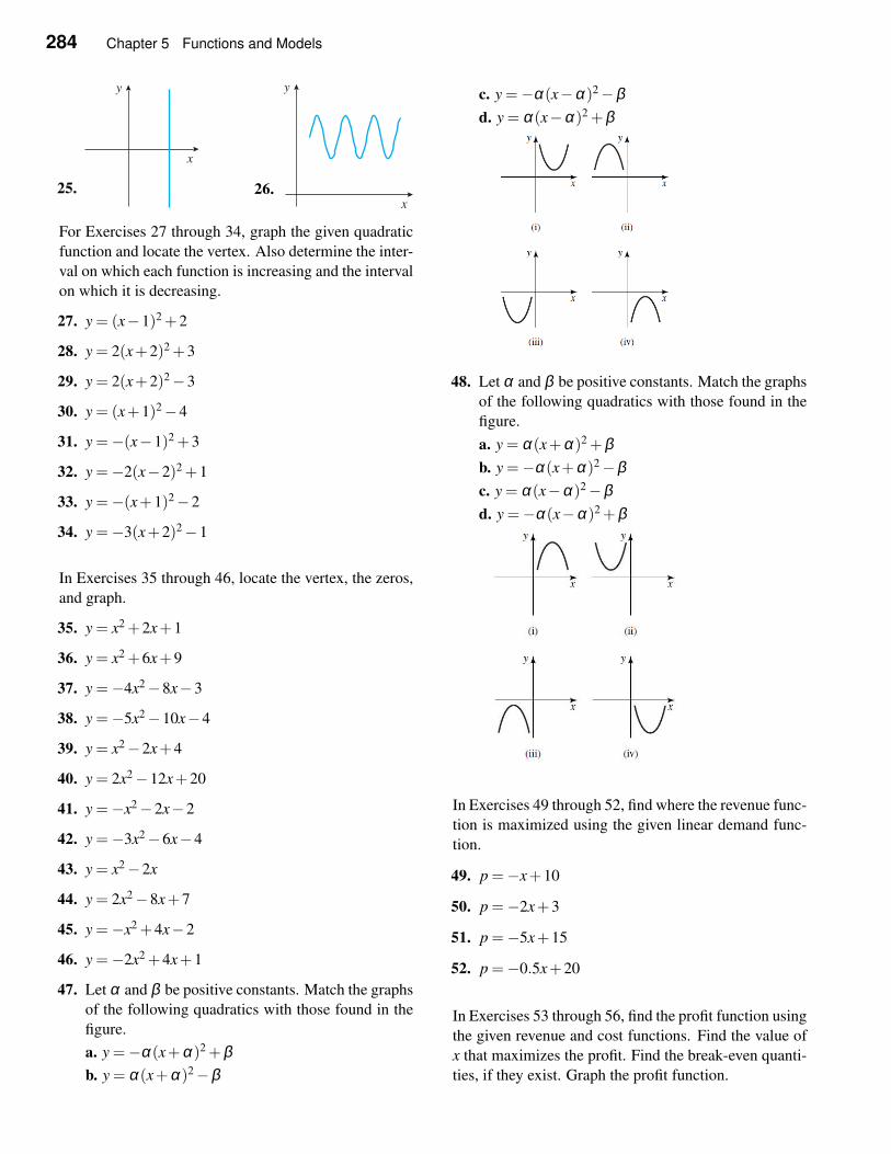
284 Chapter 5 Functions and Models
25.
y
x
26.
y
x
For Exercises 27 through 34, graph the given quadratic
function and locate the vertex. Also determine the inter-
val on which each function is increasing and the interval
on which it is decreasing.
27. y = (x−1)2 +2
28. y = 2(x+2)2 +3
29. y = 2(x+2)2−3
30. y = (x+1)2−4
31. y =−(x−1)2 +3
32. y =−2(x−2)2 +1
33. y =−(x+1)2−2
34. y =−3(x+2)2−1
In Exercises 35 through 46, locate the vertex, the zeros,
and graph.
35. y = x2 +2x+1
36. y = x2 +6x+9
37. y =−4x2−8x−3
38. y =−5x2−10x−4
39. y = x2−2x+4
40. y = 2x2−12x+20
41. y =−x2−2x−2
42. y =−3x2−6x−4
43. y = x2−2x
44. y = 2x2−8x+7
45. y =−x2 +4x−2
46. y =−2x2 +4x+1
47. Let α and β be positive constants. Match the graphs
of the following quadratics with those found in the
figure.
a. y =−α(x+α)2 +βb. y = α(x+α)2−β
c. y =−α(x−α)2−βd. y = α(x−α)2 +β
48. Let α and β be positive constants. Match the graphs
of the following quadratics with those found in the
figure.
a. y = α(x+α)2 +βb. y =−α(x+α)2−βc. y = α(x−α)2−βd. y =−α(x−α)2 +β
In Exercises 49 through 52, find where the revenue func-
tion is maximized using the given linear demand func-
tion.
49. p =−x+10
50. p =−2x+3
51. p =−5x+15
52. p =−0.5x+20
In Exercises 53 through 56, find the profit function using
the given revenue and cost functions. Find the value of
x that maximizes the profit. Find the break-even quanti-
ties, if they exist. Graph the profit function.
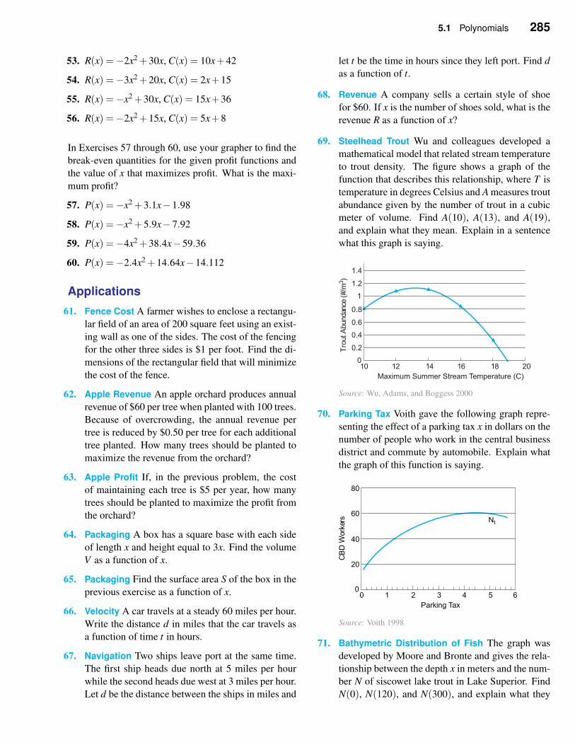
5.1 Polynomials 285
53. R(x) =−2x2 +30x, C(x) = 10x+42
54. R(x) =−3x2 +20x, C(x) = 2x+15
55. R(x) =−x2 +30x, C(x) = 15x+36
56. R(x) =−2x2 +15x, C(x) = 5x+8
In Exercises 57 through 60, use your grapher to find the
break-even quantities for the given profit functions and
the value of x that maximizes profit. What is the maxi-
mum profit?
57. P(x) =−x2 +3.1x−1.98
58. P(x) =−x2 +5.9x−7.92
59. P(x) =−4x2 +38.4x−59.36
60. P(x) =−2.4x2 +14.64x−14.112
Applications
61. Fence Cost A farmer wishes to enclose a rectangu-
lar field of an area of 200 square feet using an exist-
ing wall as one of the sides. The cost of the fencing
for the other three sides is $1 per foot. Find the di-
mensions of the rectangular field that will minimize
the cost of the fence.
62. Apple Revenue An apple orchard produces annual
revenue of $60 per tree when planted with 100 trees.
Because of overcrowding, the annual revenue per
tree is reduced by $0.50 per tree for each additional
tree planted. How many trees should be planted to
maximize the revenue from the orchard?
63. Apple Profit If, in the previous problem, the cost
of maintaining each tree is $5 per year, how many
trees should be planted to maximize the profit from
the orchard?
64. Packaging A box has a square base with each side
of length x and height equal to 3x. Find the volume
V as a function of x.
65. Packaging Find the surface area S of the box in the
previous exercise as a function of x.
66. Velocity A car travels at a steady 60 miles per hour.
Write the distance d in miles that the car travels as
a function of time t in hours.
67. Navigation Two ships leave port at the same time.
The first ship heads due north at 5 miles per hour
while the second heads due west at 3 miles per hour.
Let d be the distance between the ships in miles and
let t be the time in hours since they left port. Find d
as a function of t.
68. Revenue A company sells a certain style of shoe
for $60. If x is the number of shoes sold, what is the
revenue R as a function of x?
69. Steelhead Trout Wu and colleagues developed a
mathematical model that related stream temperature
to trout density. The figure shows a graph of the
function that describes this relationship, where T is
temperature in degrees Celsius and A measures trout
abundance given by the number of trout in a cubic
meter of volume. Find A(10), A(13), and A(19),and explain what they mean. Explain in a sentence
what this graph is saying.
Source: Wu, Adams, and Boggess 2000
70. Parking Tax Voith gave the following graph repre-
senting the effect of a parking tax x in dollars on the
number of people who work in the central business
district and commute by automobile. Explain what
the graph of this function is saying.
80
60
40
20
00 1 2 3 4 5
Nt
6
Parking Tax
srekr
oW
DB
C
Source: Voith 1998
71. Bathymetric Distribution of Fish The graph was
developed by Moore and Bronte and gives the rela-
tionship between the depth x in meters and the num-
ber N of siscowet lake trout in Lake Superior. Find
N(0), N(120), and N(300), and explain what they
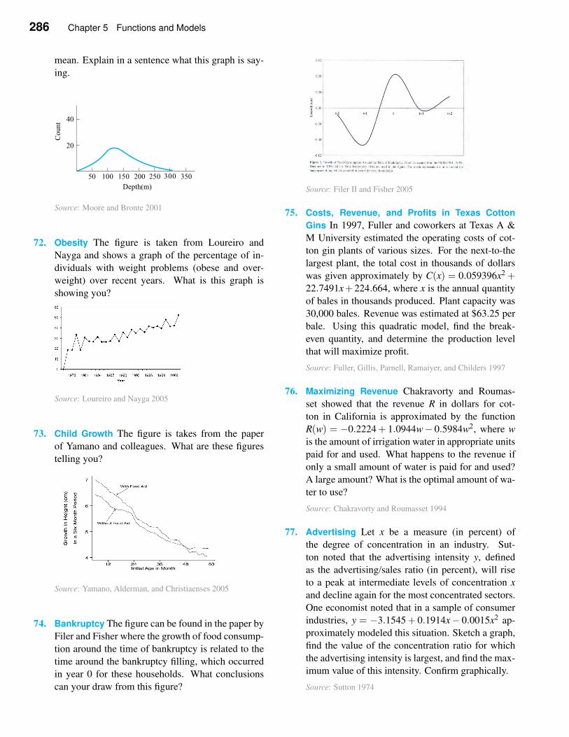
286 Chapter 5 Functions and Models
mean. Explain in a sentence what this graph is say-
ing.
50 100 150 200Depth(m)
tnuoC
300
20
40
250 350
Source: Moore and Bronte 2001
72. Obesity The figure is taken from Loureiro and
Nayga and shows a graph of the percentage of in-
dividuals with weight problems (obese and over-
weight) over recent years. What is this graph is
showing you?
Source: Loureiro and Nayga 2005
73. Child Growth The figure is takes from the paper
of Yamano and colleagues. What are these figures
telling you?
Source: Yamano, Alderman, and Christiaenses 2005
74. Bankruptcy The figure can be found in the paper by
Filer and Fisher where the growth of food consump-
tion around the time of bankruptcy is related to the
time around the bankruptcy filling, which occurred
in year 0 for these households. What conclusions
can your draw from this figure?
Source: Filer II and Fisher 2005
75. Costs, Revenue, and Profits in Texas Cotton
Gins In 1997, Fuller and coworkers at Texas A &
M University estimated the operating costs of cot-
ton gin plants of various sizes. For the next-to-the
largest plant, the total cost in thousands of dollars
was given approximately by C(x) = 0.059396x2 +22.7491x+224.664, where x is the annual quantity
of bales in thousands produced. Plant capacity was
30,000 bales. Revenue was estimated at $63.25 per
bale. Using this quadratic model, find the break-
even quantity, and determine the production level
that will maximize profit.
Source: Fuller, Gillis, Parnell, Ramaiyer, and Childers 1997
76. Maximizing Revenue Chakravorty and Roumas-
set showed that the revenue R in dollars for cot-
ton in California is approximated by the function
R(w) = −0.2224+ 1.0944w− 0.5984w2, where w
is the amount of irrigation water in appropriate units
paid for and used. What happens to the revenue if
only a small amount of water is paid for and used?
A large amount? What is the optimal amount of wa-
ter to use?
Source: Chakravorty and Roumasset 1994
77. Advertising Let x be a measure (in percent) of
the degree of concentration in an industry. Sut-
ton noted that the advertising intensity y, defined
as the advertising/sales ratio (in percent), will rise
to a peak at intermediate levels of concentration x
and decline again for the most concentrated sectors.
One economist noted that in a sample of consumer
industries, y = −3.1545+ 0.1914x− 0.0015x2 ap-
proximately modeled this situation. Sketch a graph,
find the value of the concentration ratio for which
the advertising intensity is largest, and find the max-
imum value of this intensity. Confirm graphically.
Source: Sutton 1974
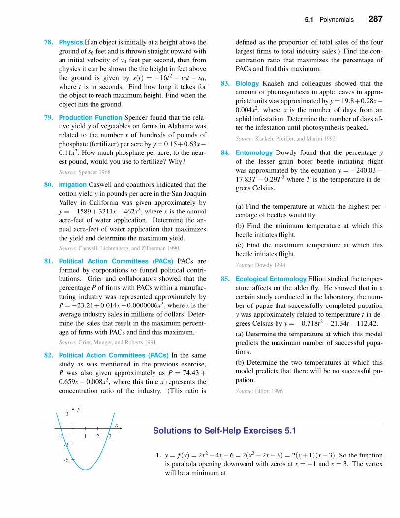
5.1 Polynomials 287
78. Physics If an object is initially at a height above the
ground of s0 feet and is thrown straight upward with
an initial velocity of v0 feet per second, then from
physics it can be shown the the height in feet above
the ground is given by s(t) = −16t2 + v0t + s0,where t is in seconds. Find how long it takes for
the object to reach maximum height. Find when the
object hits the ground.
79. Production Function Spencer found that the rela-
tive yield y of vegetables on farms in Alabama was
related to the number x of hundreds of pounds of
phosphate (fertilizer) per acre by y= 0.15+0.63x−0.11x2. How much phosphate per acre, to the near-
est pound, would you use to fertilize? Why?
Source: Spencer 1968
80. Irrigation Caswell and coauthors indicated that the
cotton yield y in pounds per acre in the San Joaquin
Valley in California was given approximately by
y = −1589+ 3211x− 462x2, where x is the annual
acre-feet of water application. Determine the an-
nual acre-feet of water application that maximizes
the yield and determine the maximum yield.
Source: Caswell, Lichtenberg, and Zilberman 1990
81. Political Action Committees (PACs) PACs are
formed by corporations to funnel political contri-
butions. Grier and collaborators showed that the
percentage P of firms with PACs within a manufac-
turing industry was represented approximately by
P =−23.21+0.014x−0.0000006x2, where x is the
average industry sales in millions of dollars. Deter-
mine the sales that result in the maximum percent-
age of firms with PACs and find this maximum.
Source: Grier, Munger, and Roberts 1991
82. Political Action Committees (PACs) In the same
study as was mentioned in the previous exercise,
P was also given approximately as P = 74.43 +0.659x− 0.008x2, where this time x represents the
concentration ratio of the industry. (This ratio is
defined as the proportion of total sales of the four
largest firms to total industry sales.) Find the con-
centration ratio that maximizes the percentage of
PACs and find this maximum.
83. Biology Kaakeh and colleagues showed that the
amount of photosynthesis in apple leaves in appro-
priate units was approximated by y= 19.8+0.28x−0.004x2, where x is the number of days from an
aphid infestation. Determine the number of days af-
ter the infestation until photosynthesis peaked.
Source: Kaakeh, Pfeiffer, and Marini 1992
84. Entomology Dowdy found that the percentage y
of the lesser grain borer beetle initiating flight
was approximated by the equation y = −240.03+17.83T −0.29T 2 where T is the temperature in de-
grees Celsius.
(a) Find the temperature at which the highest per-
centage of beetles would fly.
(b) Find the minimum temperature at which this
beetle initiates flight.
(c) Find the maximum temperature at which this
beetle initiates flight.
Source: Dowdy 1994
85. Ecological Entomology Elliott studied the temper-
ature affects on the alder fly. He showed that in a
certain study conducted in the laboratory, the num-
ber of pupae that successfully completed pupation
y was approximately related to temperature t in de-
grees Celsius by y =−0.718t2 +21.34t−112.42.
(a) Determine the temperature at which this model
predicts the maximum number of successful pupa-
tions.
(b) Determine the two temperatures at which this
model predicts that there will be no successful pu-
pation.
Source: Elliott 1996
Solutions to Self-Help Exercises 5.1
1. y = f (x) = 2x2−4x−6 = 2(x2−2x−3) = 2(x+1)(x−3). So the function
is parabola opening downward with zeros at x = −1 and x = 3. The vertex
will be a minimum at
x
-1 1 2 3
-6
-3
3y
288 Chapter 5 Functions and Models
h =− b
2a=−−(−4)
2(2)= 1 and k = c− b2
4a=−6− (−4)2
4∗2=−8
So the vertex is at (1,−8). A graph is shown in the figure.
2. The revenue function is R(x) = px = (−0.5x+ 60)x = −0.5x2 + 60x. The
vertex is at
x =−b
2a=−60
2(−0.5)= 60
Therefore 60 lockets must be sold to maximize the revenue. The rev-
enue when 60 lockets are sold is R(60) = −0.5(60)2 + 60(60) = 1800, so
the maximum revenue is $1800. To sell 60 lockets, the price must be
p(60) =−0.5(60)+60 = 30 or $30 each.
5.2 Power, Rational, and Piecewise Defined Functions
✧ Power Function
In the previous section we considered polynomials which are functions of the
form
f (x) = anxn +an−1xn−1 + · · ·+a1x+a0 (an 6= 0)
where an, an−1, . . ., a1, a0, are constants and n is a nonnegative integer. What we
will now consider are power functions where the exponent is no longer limited
to nonnegative integers.
Power Functions
A power function is a function of the form
f (x) = kxr
where k and r are real numbers.
Warning There is a substantial difference between the power function xr and
exponential function rx which we will discuss in the next section of this chapter.
The following definitions and properties are listed here as a convenient re-
view.
Some Definitions Involving Exponentials
If a 6= 0, a0 = 1, a−1 =1
a, and, in general a−x =
1
ax
a1/2 =√
a, a1/3 = 3√
a, and, in general a1/n = n√
a
am/n = n√
am = ( n√
a)m
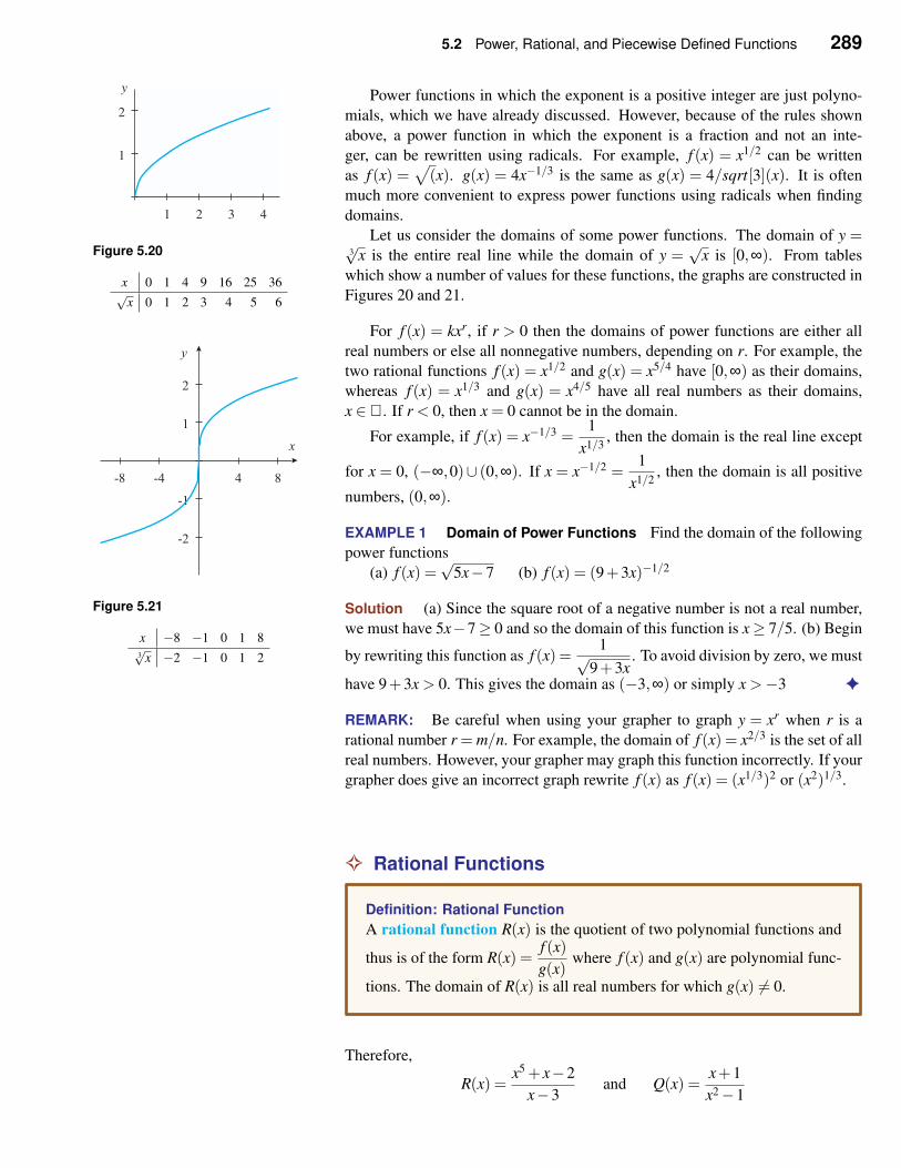
5.2 Power, Rational, and Piecewise Defined Functions 289
Power functions in which the exponent is a positive integer are just polyno-
mials, which we have already discussed. However, because of the rules shown
above, a power function in which the exponent is a fraction and not an inte-
ger, can be rewritten using radicals. For example, f (x) = x1/2 can be written
as f (x) =√
(x). g(x) = 4x−1/3 is the same as g(x) = 4/sqrt[3](x). It is often
much more convenient to express power functions using radicals when finding
domains.
y
1 2 3 4
1
2
Figure 5.20
x 0 1 4 9 16 25 36√
x 0 1 2 3 4 5 6
Let us consider the domains of some power functions. The domain of y =3√
x is the entire real line while the domain of y =√
x is [0,∞). From tables
which show a number of values for these functions, the graphs are constructed in
Figures 20 and 21.
y
x
-8 -4 4 8
-2
-1
1
2
Figure 5.21
x −8 −1 0 1 83√
x −2 −1 0 1 2
For f (x) = kxr, if r > 0 then the domains of power functions are either all
real numbers or else all nonnegative numbers, depending on r. For example, the
two rational functions f (x) = x1/2 and g(x) = x5/4 have [0,∞) as their domains,
whereas f (x) = x1/3 and g(x) = x4/5 have all real numbers as their domains,
x ∈ℜ. If r < 0, then x = 0 cannot be in the domain.
For example, if f (x) = x−1/3 =1
x1/3, then the domain is the real line except
for x = 0, (−∞,0)∪ (0,∞). If x = x−1/2 =1
x1/2, then the domain is all positive
numbers, (0,∞).
EXAMPLE 1 Domain of Power Functions Find the domain of the following
power functions
(a) f (x) =√
5x−7 (b) f (x) = (9+3x)−1/2
Solution (a) Since the square root of a negative number is not a real number,
we must have 5x−7≥ 0 and so the domain of this function is x≥ 7/5. (b) Begin
by rewriting this function as f (x) =1√
9+3x. To avoid division by zero, we must
have 9+3x > 0. This gives the domain as (−3,∞) or simply x >−3 ✦
REMARK: Be careful when using your grapher to graph y = xr when r is a
rational number r = m/n. For example, the domain of f (x) = x2/3 is the set of all
real numbers. However, your grapher may graph this function incorrectly. If your
grapher does give an incorrect graph rewrite f (x) as f (x) = (x1/3)2 or (x2)1/3.
✧ Rational Functions
Definition: Rational Function
A rational function R(x) is the quotient of two polynomial functions and
thus is of the form R(x) =f (x)
g(x)where f (x) and g(x) are polynomial func-
tions. The domain of R(x) is all real numbers for which g(x) 6= 0.
Therefore,
R(x) =x5 + x−2
x−3and Q(x) =
x+1
x2−1
290 Chapter 5 Functions and Models
are rational functions. The domain of R(x) all real numbers other than x = 3,
(−∞,3)∪ (3,∞). The domain of Q(x) is all real numbers other than x = ±1,
(−∞,−1)∪ (−1,1)∪ (1,∞).
A rational expression is a sum, difference, product or quotient of terms, each
which is the quotient of polynomials. Thus the following are rational expressions
x2 +1
x3− x−32x3 +
5x+1
x2−2
Rational expressions must satisfy the same rules as real numbers.
Rules for Rational Expressions
Let a(x), b(x), c(x), and d(x) be rational expressions with b(x) 6= 0 and
d(x) 6= 0. Also c(x) 6= 0 in Rule 4. Then
Rule 1.a(x)
b(x)± c(x)
b(x)=
a(x)± c(x)
b(x)
Rule 2.a(x)d(x)
b(x)d(x)=
a(x)
b(x)
Rule 3.a(x)
b(x)· c(x)
d(x)=
a(x)c(x)
b(x)d(x)
Rule 4.a(x)
b(x)÷ c(x)
d(x)=
a(x)d(x)
b(x)c(x)
EXAMPLE 2 Simplifying Rational Functions Simply the following rational
functions and find their domain
(a) f (x) =x2 + x+1
x2 +1− x+1
x2 +1
(b) f (x) =x2−1
x2 +4x+3
(c) f (x) =x2 +3x+2
2x2− x−1· x−1
x+1
Solution (a) Using Rule 1,
f (x) =x2 + x+1
x2 +1− x+1
x2 +1=
(x2 + x+1)− (x+1)
x2 +1=
x2
x2 +1
The domain is all real numbers, x ∈ℜ.
(b) Using Rule 2,
f (x) =x2−1
x2 +4x+3=
(x+1)(x−1)
(x+1)(x+3)=
(x−1)
(x+3)
The domain is all real numbers except x = −1 and x = −3, (−∞,−3) ∪(−3,−1)∪ (−1,∞). In Rule 2 we assumed that neither term could be zero and
so canceling the common term was allowed. Since the domain of the original
function was (−∞,−3)∪ (−3,11)∪ (11,∞) this needs to also be the domain of
the simplified function.
5.2 Power, Rational, and Piecewise Defined Functions 291
(c) Using Rule 3,
f (x) =x2 +3x+2
2x2− x−1· x−1
x+1=
(x+1)(x+2)(x−1)
(x−1)(2x+1)(x+1)=
x+2
2x+1
The domain is all real numbers except x = ±1 and x = −1
2, (−∞,−1) ∪
(−1,−1/2)∪ (−1/2,1)∪ (1,∞), for the same reason listed in part (b) ✦
If we wish to combine two rational expressions and they do not have the same
denominator, the first thing that must be done is find the least common multiple
of the two denominators. If we wish to combine the two fractions
1
x2−2x+1− 1
x3− x
we must first factor to obtain
1
x2−2x+1− 1
x3− x=
1
(x−1)2− 1
x(x−1)(x+1)
We now take as the least common denominator the product of each of the factors,
taking the power of each factor as the highest power that appears. Thus, the least
common denominator for the above example is x(x−1)2(x+1). Thus,
1
(x−1)2− 1
x(x−1)(x+1)=
1
(x−1)2
x(x+1)
x(x+1)− 1
x(x−1)(x+1)
x−1
x−1
=x(x+1)− (x−1)
x(x−1)2(x+1)
=x2 + x− x+1
x(x−1)2(x+1)=
x2 +1
x(x−1)2(x+1)
An operation often used in calculus is rationalizing a numerator or denomi-
nator as demonstrated in the following example.
EXAMPLE 3 Rationalizing the Numerator Rationalize
√x−2
x−4
Solution√
x−2
x−4=
√x−2
x−4
√x+2√x+2
=(√
x)2− (2)2
(x−4)(√
x+2)=
1√x+2
✦
EXAMPLE 4 An expression from calculus Simplify the difference quotient,f (x+h)− f (x)
h, for the following functions
(a) f (x) = 2x2 + x+1 (b) f (x) =1
x(c) f (x) =
√3x−1
Solution (a)
f (x+h)− f (x)
h=
1
h
[(2(x+h)2 +(x+h)+1
)−(2x2 + x+1
)]
=1
h
[2x2 +4xh+2h2 + x+h+1−2x2− x−1
]
=4xh+h+2h2
h
= 4x+1+h
292 Chapter 5 Functions and Models
(b)
f (x+h)− f (x)
h=
1
h
[1
x+h− 1
x
]
=1
h
[1
x+h· x
x− 1
x· x+h
x+h
]
=1
h
[x− (x+h)
x(x+h)
]
=−h
xh(x+h)=
−1
x(x+h)
(c)f (x+h)− f (x)
h=
1
h
[√
3(x+h)−1−√
3x−1]
=1
h
[√
3(x+h)−1−√
3x−1]
·√
3(x+h)−1+√
3x−1√
3(x+h)−1+√
3x−1
=1
h
[
3x+3h−1− (3x−1)√
3(x+h)−1+√
3x−1
]
=1
h
[
3h√
3(x+h)−1+√
3x−1
]
=3
√
3(x+h)−1+√
3x−1
In each of these difference quotients the h in the denominator cancels out.
This will be quite important when these expressions are used in calculus. ✦
✧ Piecewise Functions
We often encounter functions with domains divided into two or more parts
with a different rule applied to each part. We call such functions piecewise-
defined functions. The absolute value function, |x|, is such an example.
Definition of Absolute Value Function, |x|
|x|={
x if x≥ 0
−x if x < 0
For example, since −5 < 0, | − 5| = −(−5) = 5. Do not make the mistake
of thinking that the absolute value of an algebraic expression can be obtained by
“dropping the sign.”
We now determine the graphs of two piecewise-defined functions.
EXAMPLE 5 The Graph of the Absolute Value Function Graph the function
y = f (x) = |x|.
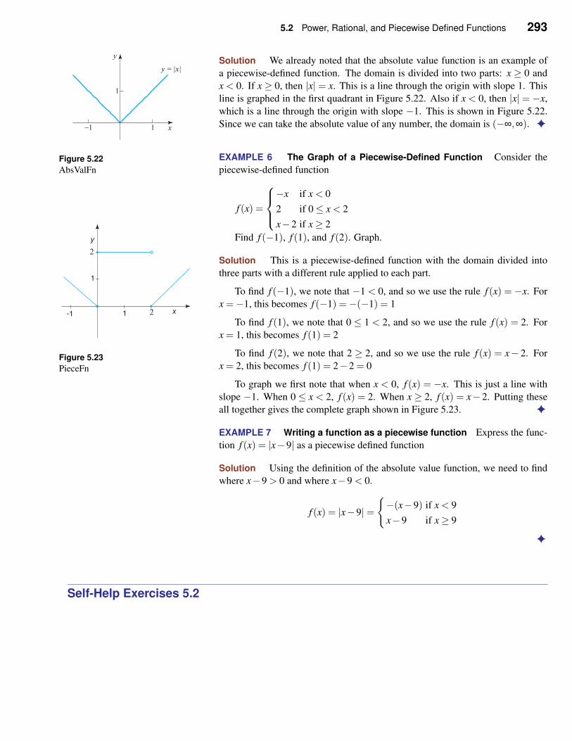
5.2 Power, Rational, and Piecewise Defined Functions 293
Solution We already noted that the absolute value function is an example of
a piecewise-defined function. The domain is divided into two parts: x ≥ 0 and
x < 0. If x ≥ 0, then |x| = x. This is a line through the origin with slope 1. This
line is graphed in the first quadrant in Figure 5.22. Also if x < 0, then |x| = −x,
which is a line through the origin with slope −1. This is shown in Figure 5.22.
Since we can take the absolute value of any number, the domain is (−∞,∞). ✦x
y
y = |x |
-1 1
1
Figure 5.22
AbsValFn
EXAMPLE 6 The Graph of a Piecewise-Defined Function Consider the
piecewise-defined function
f (x) =
−x if x < 0
2 if 0≤ x < 2
x−2 if x≥ 2
Find f (−1), f (1), and f (2). Graph.
Solution This is a piecewise-defined function with the domain divided into
three parts with a different rule applied to each part.
To find f (−1), we note that −1 < 0, and so we use the rule f (x) = −x. For
x =−1, this becomes f (−1) =−(−1) = 1
To find f (1), we note that 0 ≤ 1 < 2, and so we use the rule f (x) = 2. For
x = 1, this becomes f (1) = 2
Figure 5.23
PieceFn
To find f (2), we note that 2 ≥ 2, and so we use the rule f (x) = x− 2. For
x = 2, this becomes f (1) = 2−2 = 0
To graph we first note that when x < 0, f (x) = −x. This is just a line with
slope −1. When 0 ≤ x < 2, f (x) = 2. When x ≥ 2, f (x) = x− 2. Putting these
all together gives the complete graph shown in Figure 5.23. ✦
EXAMPLE 7 Writing a function as a piecewise function Express the func-
tion f (x) = |x−9| as a piecewise defined function
Solution Using the definition of the absolute value function, we need to find
where x−9 > 0 and where x−9 < 0.
f (x) = |x−9|={
−(x−9) if x < 9
x−9 if x≥ 9
✦
Self-Help Exercises 5.2
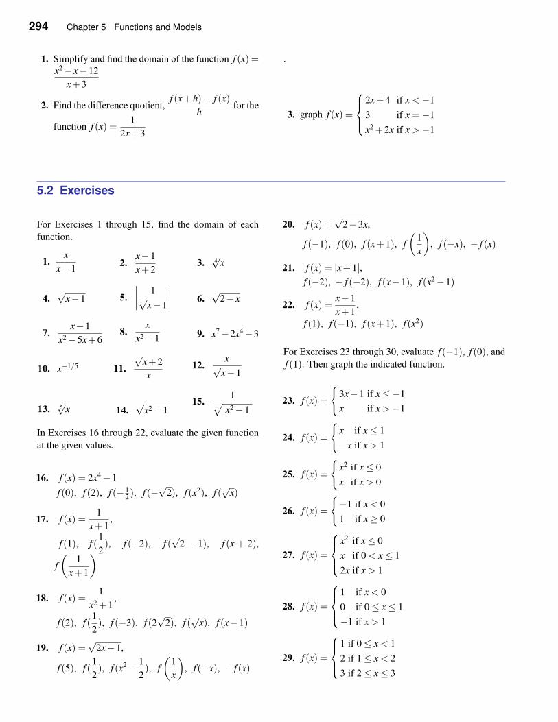
294 Chapter 5 Functions and Models
1. Simplify and find the domain of the function f (x) =x2− x−12
x+3
2. Find the difference quotient,f (x+h)− f (x)
hfor the
function f (x) =1
2x+3
.
3. graph f (x) =
2x+4 if x <−1
3 if x =−1
x2 +2x if x >−1
5.2 Exercises
For Exercises 1 through 15, find the domain of each
function.
1.x
x−12.
x−1
x+23. 4√
x
4.√
x−1 5.
∣∣∣∣
1√x−1
∣∣∣∣ 6.
√2− x
7.x−1
x2−5x+68.
x
x2−19. x7−2x4−3
10. x−1/5 11.
√x+2
x12.
x√x−1
13. 5√
x 14.√
x2−115.
1√
|x2−1|
In Exercises 16 through 22, evaluate the given function
at the given values.
16. f (x) = 2x4−1
f (0), f (2), f (− 12), f (−
√2), f (x2), f (
√x)
17. f (x) =1
x+1,
f (1), f (1
2), f (−2), f (
√2 − 1), f (x + 2),
f
(1
x+1
)
18. f (x) =1
x2 +1,
f (2), f (1
2), f (−3), f (2
√2), f (
√x), f (x−1)
19. f (x) =√
2x−1,
f (5), f (1
2), f (x2− 1
2), f
(1
x
)
, f (−x), − f (x)
20. f (x) =√
2−3x,
f (−1), f (0), f (x+1), f
(1
x
)
, f (−x), − f (x)
21. f (x) = |x+1|,f (−2), − f (−2), f (x−1), f (x2−1)
22. f (x) =x−1
x+1,
f (1), f (−1), f (x+1), f (x2)
For Exercises 23 through 30, evaluate f (−1), f (0), and
f (1). Then graph the indicated function.
23. f (x) =
{
3x−1 if x≤−1
x if x >−1
24. f (x) =
{
x if x≤ 1
−x if x > 1
25. f (x) =
{
x2 if x≤ 0
x if x > 0
26. f (x) =
{
−1 if x < 0
1 if x≥ 0
27. f (x) =
x2 if x≤ 0
x if 0 < x≤ 1
2x if x > 1
28. f (x) =
1 if x < 0
0 if 0≤ x≤ 1
−1 if x > 1
29. f (x) =
1 if 0≤ x < 1
2 if 1≤ x < 2
3 if 2≤ x≤ 3
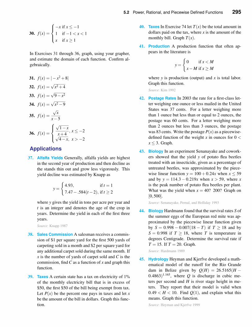
5.2 Power, Rational, and Piecewise Defined Functions 295
30. f (x) =
−x if x≤−1
1 if −1 < x < 1
x if x≥ 1
In Exercises 31 through 36, graph, using your grapher,
and estimate the domain of each function. Confirm al-
gebraically.
31. f (x) = |− x2 +8|
32. f (x) =√
x2 +4
33. f (x) =√
9− x2
34. f (x) =√
x2−9
35. f (x) =
√x
x−5
36. f (x) =
√1− x
x+4, x≤−2
√4− x, x >−2
Applications
37. Alfalfa Yields Generally, alfalfa yields are highest
in the second year of production and then decline as
the stands thin out and grow less vigorously. This
yield decline was estimated by Knapp as
y =
{
4.93, if t = 1
7.47− .584(t−2), if t ≥ 2
where y gives the yield in tons per acre per year and
t is an integer and denotes the age of the crop in
years. Determine the yield in each of the first three
years.
Source: Knapp 1987
38. Sales Commission A salesman receives a commis-
sion of $1 per square yard for the first 500 yards of
carpeting sold in a month and $2 per square yard for
any additional carpet sold during the same month. If
x is the number of yards of carpet sold and C is the
commission, find C as a function of x and graph this
function.
39. Taxes A certain state has a tax on electricity of 1%
of the monthly electricity bill that is in excess of
$50, the first $50 of the bill being exempt from tax.
Let P(x) be the percent one pays in taxes and let x
be the amount of the bill in dollars. Graph this func-
tion.
40. Taxes In Exercise 74 let T (x) be the total amount in
dollars paid on the tax, where x is the amount of the
monthly bill. Graph T (x).
41. Production A production function that often ap-
pears in the literature is
y =
{
0 if x < M
x−M if x≥M
where y is production (output) and x is total labor.
Graph this function.
Source: Kim 1992
42. Postage Rates In 2003 the rate for a first-class let-
ter weighing one ounce or less mailed in the United
States was 37 cents. For a letter weighing more
than 1 ounce but less than or equal to 2 ounces, the
postage was 60 cents. For a letter weighing more
than 2 ounces but less than 3 ounces, the postage
was 83 cents. Write the postage P(x) as a piecewise-
defined function of the weight x in ounces for 0 <x≤ 3. Graph.
43. Biology In an experiment Senanayake and cowork-
ers showed that the yield y of potato flea beetles
treated with an insecticide, given as a percentage of
untreated beetles, was approximated by the piece-
wise linear function y = 100+ 0.24x when x ≤ 59
and by y = 114.3− 0.219x when x > 59, where x
is the peak number of potato flea beetles per plant.
What was the yield when x = 40? 200? Graph on
[0,500].
Source: Senanayake, Pernal, and Holliday 1993
44. Biology Hardmann found that the survival rates S of
the summer eggs of the European red mite was ap-
proximated by the piecewise linear function given
by S = 0.998− 0.007(18− T ) if T ≥ 18 and by
S = 0.998 if T ≥ 18, where T is temperature in
degrees Centigrade. Determine the survival rate if
T = 15. If T = 20. Graph.
Source: Hardmann 1989
45. Hydrology Heyman and Kjerfve developed a math-
ematical model of the runoff for the Rio Grande
dam in Belize given by Q(H) = 26.5165(H −0.4863)1.165, where Q is discharge in cubic me-
ters per second and H is river stage height in me-
ters. They report that their model is valid when
0.49 < H < 10. Find Q(1), and explain what this
means. Graph this function.
Source: Heyman and Kjerfve 1999
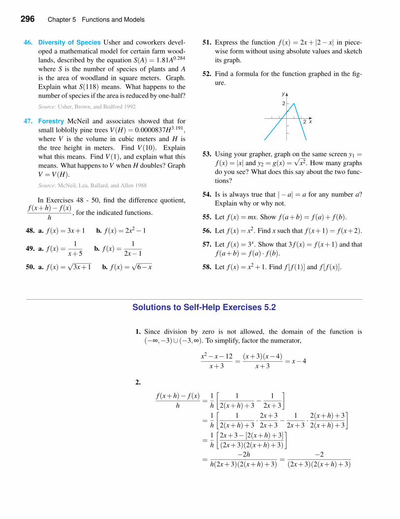
296 Chapter 5 Functions and Models
46. Diversity of Species Usher and coworkers devel-
oped a mathematical model for certain farm wood-
lands, described by the equation S(A) = 1.81A0.284
where S is the number of species of plants and A
is the area of woodland in square meters. Graph.
Explain what S(118) means. What happens to the
number of species if the area is reduced by one-half?
Source: Usher, Brown, and Bedford 1992
47. Forestry McNeil and associates showed that for
small loblolly pine trees V (H) = 0.0000837H3.191,where V is the volume in cubic meters and H is
the tree height in meters. Find V (10). Explain
what this means. Find V (1), and explain what this
means. What happens to V when H doubles? Graph
V =V (H).
Source: McNeil, Lea, Ballard, and Allen 1988
In Exercises 48 - 50, find the difference quotient,f (x+h)− f (x)
h, for the indicated functions.
48. a. f (x) = 3x+1 b. f (x) = 2x2−1
49. a. f (x) =1
x+5b. f (x) =
1
2x−1
50. a. f (x) =√
3x+1 b. f (x) =√
6− x
51. Express the function f (x) = 2x+ |2− x| in piece-
wise form without using absolute values and sketch
its graph.
52. Find a formula for the function graphed in the fig-
ure.
53. Using your grapher, graph on the same screen y1 =f (x) = |x| and y2 = g(x) =
√x2. How many graphs
do you see? What does this say about the two func-
tions?
54. Is is always true that | − a| = a for any number a?
Explain why or why not.
55. Let f (x) = mx. Show f (a+b) = f (a)+ f (b).
56. Let f (x) = x2. Find x such that f (x+1) = f (x+2).
57. Let f (x) = 3x. Show that 3 f (x) = f (x+1) and that
f (a+b) = f (a) · f (b).
58. Let f (x) = x2 +1. Find f [ f (1)] and f [ f (x)].
Solutions to Self-Help Exercises 5.2
1. Since division by zero is not allowed, the domain of the function is
(−∞,−3)∪ (−3,∞). To simplify, factor the numerator,
x2− x−12
x+3=
(x+3)(x−4)
x+3= x−4
2.
f (x+h)− f (x)
h=
1
h
[1
2(x+h)+3− 1
2x+3
]
=1
h
[1
2(x+h)+3· 2x+3
2x+3− 1
2x+3· 2(x+h)+3
2(x+h)+3
]
=1
h
[2x+3− [2(x+h)+3]
(2x+3)(2(x+h)+3)
]
=−2h
h(2x+3)(2(x+h)+3)=
−2
(2x+3)(2(x+h)+3)
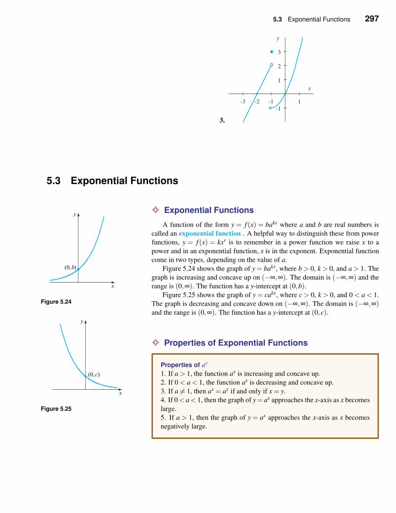
5.3 Exponential Functions 297
3.
-3 -2 -1 1
-1
1
2
3
y
x
5.3 Exponential Functions
✧ Exponential Functions
A function of the form y = f (x) = bakx where a and b are real numbers is
called an exponential function . A helpful way to distinguish these from power
functions, y = f (x) = kxr is to remember in a power function we raise x to a
power and in an exponential function, x is in the exponent. Exponential function
come in two types, depending on the value of a.
Figure 5.24 shows the graph of y = bakx, where b > 0, k > 0, and a > 1. The
graph is increasing and concave up on (−∞,∞). The domain is (−∞,∞) and the
range is (0,∞). The function has a y-intercept at (0,b).x
y
(0,b)
Figure 5.24Figure 5.25 shows the graph of y = cakx, where c > 0, k > 0, and 0 < a < 1.
The graph is decreasing and concave down on (−∞,∞). The domain is (−∞,∞)and the range is (0,∞). The function has a y-intercept at (0,c).
x
y
(0,c)
Figure 5.25
✧ Properties of Exponential Functions
Properties of ax
1. If a > 1, the function ax is increasing and concave up.
2. If 0 < a < 1, the function ax is decreasing and concave up.
3. If a 6= 1, then ax = ay if and only if x = y.
4. If 0< a< 1, then the graph of y= ax approaches the x-axis as x becomes
large.
5. If a > 1, then the graph of y = ax approaches the x-axis as x becomes
negatively large.
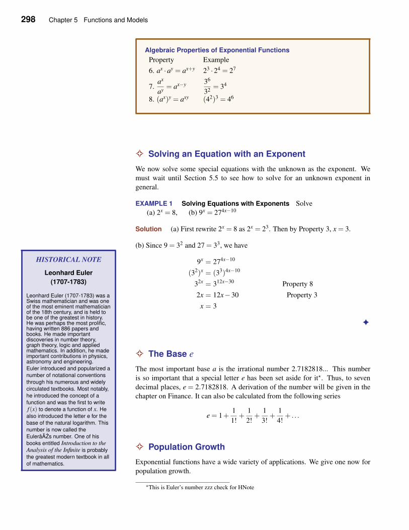
298 Chapter 5 Functions and Models
Algebraic Properties of Exponential Functions
Property Example
6. ax ·ay = ax+y 23 ·24 = 27
7.ax
ay= ax−y 36
32= 34
8. (ax)y = axy (42)3 = 46
✧ Solving an Equation with an Exponent
We now solve some special equations with the unknown as the exponent. We
must wait until Section 5.5 to see how to solve for an unknown exponent in
general.
EXAMPLE 1 Solving Equations with Exponents Solve
(a) 2x = 8, (b) 9x = 274x−10
Solution (a) First rewrite 2x = 8 as 2x = 23. Then by Property 3, x = 3.
(b) Since 9 = 32 and 27 = 33, we have
9x = 274x−10
(32)x = (33)4x−10
32x = 312x−30 Property 8
2x = 12x−30 Property 3
x = 3
✦
✧ The Base e
HISTORICAL NOTE
Leonhard Euler
(1707-1783)
Leonhard Euler (1707-1783) was aSwiss mathematician and was oneof the most eminent mathematicianof the 18th century, and is held tobe one of the greatest in history.He was perhaps the most prolific,having written 886 papers andbooks. He made importantdiscoveries in number theory,graph theory, logic and appliedmathematics. In addition, he madeimportant contributions in physics,astronomy and engineering.
Euler introduced and popularized a
number of notational conventions
through his numerous and widely
circulated textbooks. Most notably,
he introduced the concept of a
function and was the first to write
f (x) to denote a function of x. He
also introduced the letter e for the
base of the natural logarithm. This
number is now called the
EulerâAZs number. One of his
books entitled Introduction to the
Analysis of the Infinite is probably
the greatest modern textbook in all
of mathematics.
The most important base a is the irrational number 2.7182818... This number
is so important that a special letter e has been set aside for it⋆. Thus, to seven
decimal places, e = 2.7182818. A derivation of the number will be given in the
chapter on Finance. It can also be calculated from the following series
e = 1+1
1!+
1
2!+
1
3!+
1
4!+ . . .
✧ Population Growth
Exponential functions have a wide variety of applications. We give one now for
population growth.
⋆This is Euler’s number zzz check for HNote
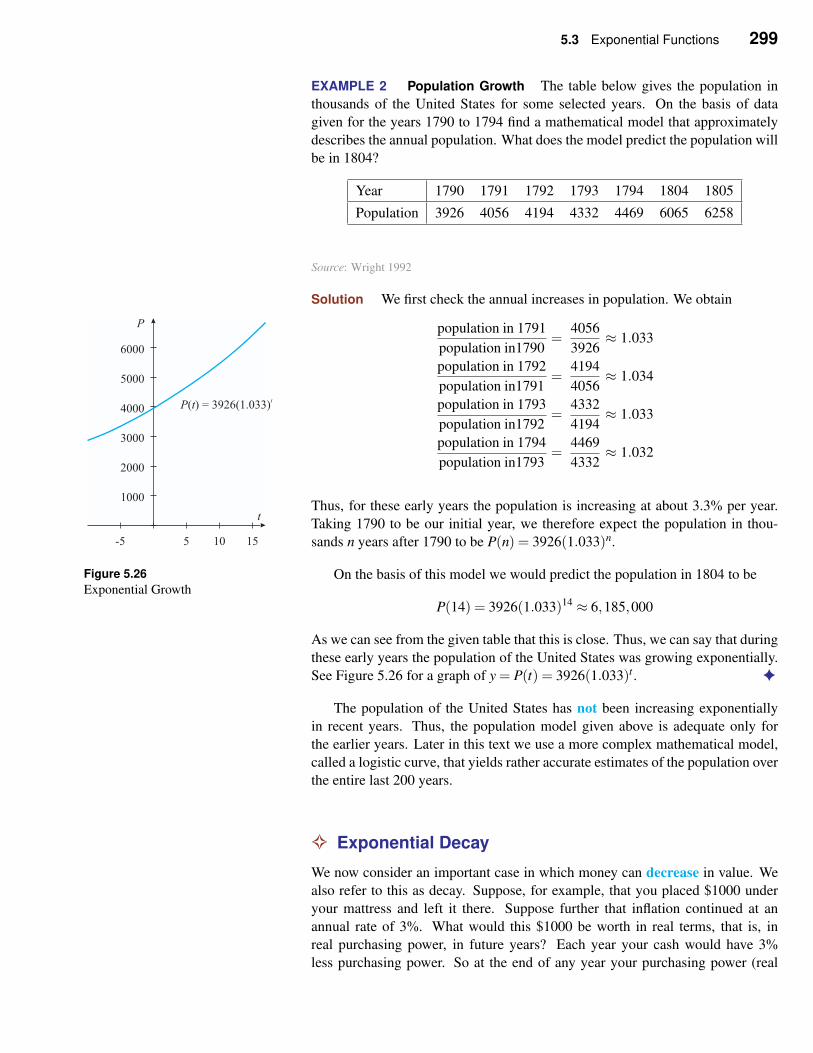
5.3 Exponential Functions 299
EXAMPLE 2 Population Growth The table below gives the population in
thousands of the United States for some selected years. On the basis of data
given for the years 1790 to 1794 find a mathematical model that approximately
describes the annual population. What does the model predict the population will
be in 1804?
Year 1790 1791 1792 1793 1794 1804 1805
Population 3926 4056 4194 4332 4469 6065 6258
Source: Wright 1992
Solution We first check the annual increases in population. We obtain
population in 1791
population in1790=
4056
3926≈ 1.033
population in 1792
population in1791=
4194
4056≈ 1.034
population in 1793
population in1792=
4332
4194≈ 1.033
population in 1794
population in1793=
4469
4332≈ 1.032
Thus, for these early years the population is increasing at about 3.3% per year.
Taking 1790 to be our initial year, we therefore expect the population in thou-
sands n years after 1790 to be P(n) = 3926(1.033)n.-5 5 10 15
1000
2000
3000
4000
5000
6000
P
t
P t( ) = 3926(1.033)t
Figure 5.26
Exponential GrowthOn the basis of this model we would predict the population in 1804 to be
P(14) = 3926(1.033)14 ≈ 6,185,000
As we can see from the given table that this is close. Thus, we can say that during
these early years the population of the United States was growing exponentially.
See Figure 5.26 for a graph of y = P(t) = 3926(1.033)t . ✦
The population of the United States has not been increasing exponentially
in recent years. Thus, the population model given above is adequate only for
the earlier years. Later in this text we use a more complex mathematical model,
called a logistic curve, that yields rather accurate estimates of the population over
the entire last 200 years.
✧ Exponential Decay
We now consider an important case in which money can decrease in value. We
also refer to this as decay. Suppose, for example, that you placed $1000 under
your mattress and left it there. Suppose further that inflation continued at an
annual rate of 3%. What would this $1000 be worth in real terms, that is, in
real purchasing power, in future years? Each year your cash would have 3%
less purchasing power. So at the end of any year your purchasing power (real
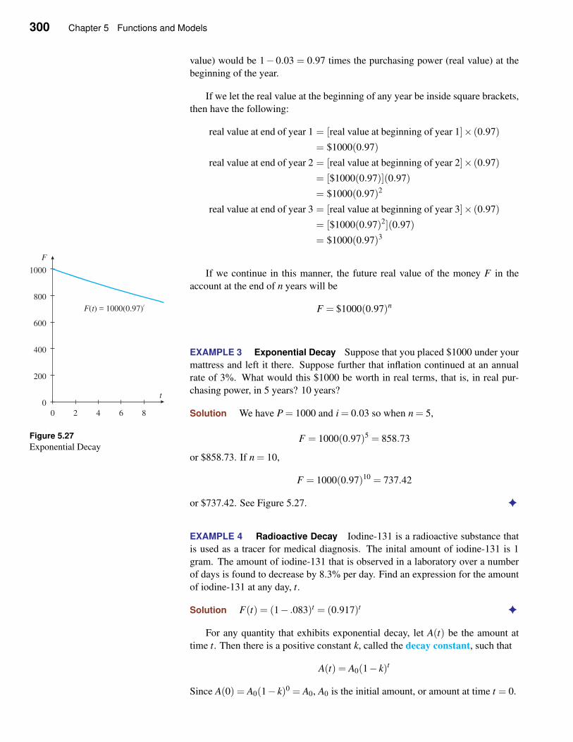
300 Chapter 5 Functions and Models
value) would be 1− 0.03 = 0.97 times the purchasing power (real value) at the
beginning of the year.
If we let the real value at the beginning of any year be inside square brackets,
then have the following:
real value at end of year 1 = [real value at beginning of year 1]× (0.97)
= $1000(0.97)
real value at end of year 2 = [real value at beginning of year 2]× (0.97)
= [$1000(0.97)](0.97)
= $1000(0.97)2
real value at end of year 3 = [real value at beginning of year 3]× (0.97)
= [$1000(0.97)2](0.97)
= $1000(0.97)3
If we continue in this manner, the future real value of the money F in the
account at the end of n years will be
F = $1000(0.97)n
EXAMPLE 3 Exponential Decay Suppose that you placed $1000 under your
mattress and left it there. Suppose further that inflation continued at an annual
rate of 3%. What would this $1000 be worth in real terms, that is, in real pur-
chasing power, in 5 years? 10 years?
Solution We have P = 1000 and i = 0.03 so when n = 5,0 2 4 6 8
0
200
400
600
800
1000
F
t
F t( ) = 1000(0.97)t
Figure 5.27
Exponential DecayF = 1000(0.97)5 = 858.73
or $858.73. If n = 10,
F = 1000(0.97)10 = 737.42
or $737.42. See Figure 5.27. ✦
EXAMPLE 4 Radioactive Decay Iodine-131 is a radioactive substance that
is used as a tracer for medical diagnosis. The inital amount of iodine-131 is 1
gram. The amount of iodine-131 that is observed in a laboratory over a number
of days is found to decrease by 8.3% per day. Find an expression for the amount
of iodine-131 at any day, t.
Solution F(t) = (1− .083)t = (0.917)t ✦
For any quantity that exhibits exponential decay, let A(t) be the amount at
time t. Then there is a positive constant k, called the decay constant, such that
A(t) = A0(1− k)t
Since A(0) = A0(1− k)0 = A0, A0 is the initial amount, or amount at time t = 0.
5.3 Exponential Functions 301
In an analogous manner for any quantity that exhibits exponential growth,
such as population growth, let A(t) be the amount at time t. Then there is a
positive constant c, called the growth constant, such that
A(t) = A0(1+ c)t
Since A(0) = A0(1+ c)0 = A0, A0 is the initial amount, or amount at time t = 0.
Self-Help Exercises 5.3
1. Solve 32x+1 =1
3x. 2. You purchase a painting for $800 which goes up in
value 5% every year. Find a formula that allows you
to find the value of the painting in the future.
5.3 Exercises
In Exercises 1 through 8, sketch a graph of each of
the functions without using your grapher. Then support
your answer with your grapher.
1. y = 5x 2. y = 7x
3. y = 3x24. y = 3−x2
5. y = (1/2)x 6. y = (0.1)x
7. y = 10x 8. y = 5−x
In Exercises 9 through 16, solve for x.
9. 3x = 9
10. 4x = 8
11. 16x = 8
12.
(1
2
)x
=1
16
13.
(1
16
)x
=1
8
14.
(1
4
)x
= 8
15. 42x = 89x+15
16. 53x = 1254x−4
In Exercises 17 through 24, graph each of the functions
without using a grapher. Then support your answer with
a grapher.
17. y = 23x
18. y = 3−2x
19. y = 3x3
20. y = 5−x2
21. y = 2−3−x
22. y = 2+3−x
23. y = 12(3
x +3−x)
24. y = 12(2
x−2−x)
In Exercises 25 through 38, solve for x.
25. 3x = 1/3
26. 5x = 1/25
27. 2x = 1/8
28. 25x = 2x+8
29. (3x+1)2 = 3
30. 52x−15x = 1/5x
31. 3x+1 = 1/3x
32. 7x2+2x = 7−x
33. 3−x2+2x = 3
34. x2x = 2x
302 Chapter 5 Functions and Models
35. 3−x(x+1) = 0
36. x252x = 52x
37. x5−x = x25−x
38. (x2 + x−2)2x = 0
Applications
39. Real Estate Appreciation The United States paid
about 4 cents an acre for the Louisiana Purchase in
1803. Suppose the value of this property grew at
an annual rate of 5.5% compounded annually. What
would an acre have been worth in 2010? Does this
seem realistic?
40. Real Estate Appreciation Redo the previous exer-
cise using a rate of 6% instead of 5.5%. Compare
this answer to the answer to the previous exercise
41. Inflation Inflation, as measured by the U.S con-
sumer price index increased by 2.8% in the year
2001. If this rate were to continue for the next 10
years, what would be the real value of $1000 after
10 years?
Source: http://www.bls.gov/ 2002
42. Inflation Inflation, as measured by the U.S con-
sumer price index, increased by 2.8% in the year
2001. If this rate were to continue for the next
10 years, use your computer or graphing calculator
to determine how long before the value of a dollar
would be reduced to 90 cents.
Source: http://www.bls.gov/ 2002
43. Deflation Inflation, as measured by Japan’s con-
sumer price index decreased (thus the word defla-
tion) by 0.7% in the year 2001. If this rate were
to continue for the next 10 years, use your computer
or graphing calculator to determine how long before
the value of a typical item would be reduced to 95%
of its value in 2001.
Source: http://www.jinjapan.org/stat/stats/05ECN32.htm 2001
44. Real Yield Suppose you were one of the people who
in 1955 purchased a 40-year Treasury bond with
a coupon rate of 3% per year. Presumably, you
thought that inflation over the next 40 years would
be low. (The inflation rate for the 30 years before
1955 was just a little over 1% a year.) In fact, the
inflation rate for the 40-year period of this bond was
4.4% a year. Thus, in real terms you would have lost
1.4% a year. If you bought $1000 of such a bond at
issuance and held it to maturity, how much would
the $1000 bond have been worth in real terms?
Source: of Atlanta 1998
45. Population of the World The human population of
the world was about 6 billion in the year 2000 and
increasing at the rate of 1.3% a year. Assume that
this population will continue to grow exponentially
at this rate, and use your computer or graphing cal-
culator to determine the year in which the popula-
tion of the world will reach 7 billion.
Source: Report 1999
46. Population of the World The human population of
the world was about 6 billion in the year 2000 and
increasing at the rate of 1.3% a year Assume that
this population will continue to grow exponentially
at this rate, and determine the population of the
world in the year 2010.
Source: Report 1999
47. Population of the Latvia The population of Latvia
was decreasing at the rate of 0.52% a year from
1995 to 2000. Assuming that the population contin-
ued to decline at this annual rate, use your computer
or graphing calculator to determine how long until
the population of Latvia will become 95% of what
is was in the year 2000.
Source: Report 1999
48. Population of the Bulgaria The population of Bul-
garia was decreasing at the rate of 0.47% a year
from 1995 to 2000. Assuming that the population
continued to decline at this annual rate, determine
the total percentage drop in population over the sub-
sequent 10 years.
Source: Report 1999
49. Radioactive Decay Plutonium-239 is a product of
nuclear reactors with a half-life of about 24,000
years. What percentage of a given sample will re-
main after 10,000 years?
50. Medicine As we noted in the text, radioactive trac-
ers are used for medical diagnosis. Suppose 20 units
of iodine-131 are shipped and take two days to ar-
rive. Determine how much of the substance arrives.
51. Medicine Suppose that 20 units of iodine-131 are
needed in two days. Determine how much should
be ordered.
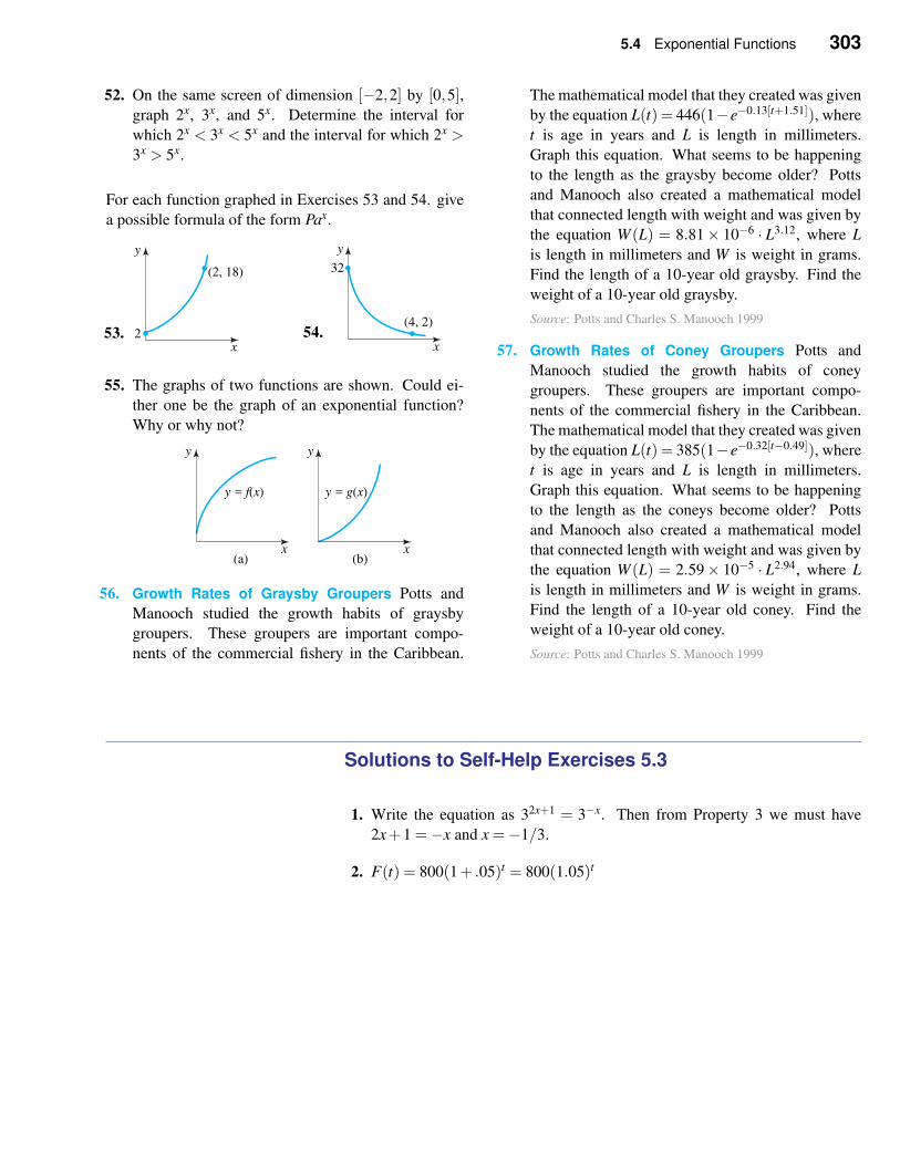
5.4 Exponential Functions 303
52. On the same screen of dimension [−2,2] by [0,5],graph 2x, 3x, and 5x. Determine the interval for
which 2x < 3x < 5x and the interval for which 2x >3x > 5x.
For each function graphed in Exercises 53 and 54. give
a possible formula of the form Pax.
53.x
y
(2, 18)
2 54.x
y
(4, 2)
32
55. The graphs of two functions are shown. Could ei-
ther one be the graph of an exponential function?
Why or why not?
x
y
x
y
y f x= ( )
(a) (b)
y g x= ( )
56. Growth Rates of Graysby Groupers Potts and
Manooch studied the growth habits of graysby
groupers. These groupers are important compo-
nents of the commercial fishery in the Caribbean.
The mathematical model that they created was given
by the equation L(t) = 446(1−e−0.13[t+1.51]), where
t is age in years and L is length in millimeters.
Graph this equation. What seems to be happening
to the length as the graysby become older? Potts
and Manooch also created a mathematical model
that connected length with weight and was given by
the equation W (L) = 8.81× 10⁻⁶ · L3.12, where L
is length in millimeters and W is weight in grams.
Find the length of a 10-year old graysby. Find the
weight of a 10-year old graysby.
Source: Potts and Charles S. Manooch 1999
57. Growth Rates of Coney Groupers Potts and
Manooch studied the growth habits of coney
groupers. These groupers are important compo-
nents of the commercial fishery in the Caribbean.
The mathematical model that they created was given
by the equation L(t) = 385(1−e−0.32[t−0.49]), where
t is age in years and L is length in millimeters.
Graph this equation. What seems to be happening
to the length as the coneys become older? Potts
and Manooch also created a mathematical model
that connected length with weight and was given by
the equation W (L) = 2.59× 10⁻⁵ · L2.94, where L
is length in millimeters and W is weight in grams.
Find the length of a 10-year old coney. Find the
weight of a 10-year old coney.
Source: Potts and Charles S. Manooch 1999
Solutions to Self-Help Exercises 5.3
1. Write the equation as 32x+1 = 3−x. Then from Property 3 we must have
2x+1 =−x and x =−1/3.
2. F(t) = 800(1+ .05)t = 800(1.05)t
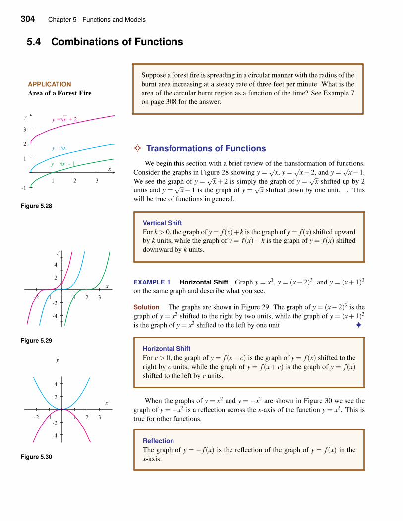
304 Chapter 5 Functions and Models
5.4 Combinations of Functions
APPLICATION
Area of a Forest Fire
Suppose a forest fire is spreading in a circular manner with the radius of the
burnt area increasing at a steady rate of three feet per minute. What is the
area of the circular burnt region as a function of the time? See Example 7
on page 308 for the answer.
✧ Transformations of Functions
We begin this section with a brief review of the transformation of functions.
Consider the graphs in Figure 28 showing y =√
x, y =√
x+2, and y =√
x−1.
We see the graph of y =√
x+ 2 is simply the graph of y =√
x shifted up by 2
units and y =√
x− 1 is the graph of y =√
x shifted down by one unit. . This
y
x
1 2 3-1
1
2
3
y = x√ + 2
y = x√
y = x√ 1-
Figure 5.28will be true of functions in general.
Vertical Shift
For k > 0, the graph of y = f (x)+k is the graph of y = f (x) shifted upward
by k units, while the graph of y = f (x)− k is the graph of y = f (x) shifted
downward by k units.
EXAMPLE 1 Horizontal Shift Graph y = x3, y = (x− 2)3, and y = (x+ 1)3
on the same graph and describe what you see.
Solution The graphs are shown in Figure 29. The graph of y = (x−2)3 is the
graph of y = x3 shifted to the right by two units, while the graph of y = (x+1)3
is the graph of y = x3 shifted to the left by one unit ✦
y
x
-2 -1 1 2 3
-4
-2
2
4
Figure 5.29
Horizontal Shift
For c > 0, the graph of y = f (x− c) is the graph of y = f (x) shifted to the
right by c units, while the graph of y = f (x+ c) is the graph of y = f (x)shifted to the left by c units.
When the graphs of y = x2 and y = −x2 are shown in Figure 30 we see the
graph of y = −x2 is a reflection across the x-axis of the function y = x2. This is
true for other functions.
x
-2 -1 1 2 3
-4
-2
2
4
y
Figure 5.30
Reflection
The graph of y = − f (x) is the reflection of the graph of y = f (x) in the
x-axis.
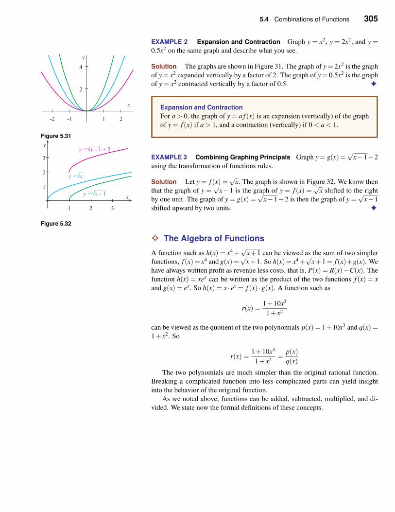
5.4 Combinations of Functions 305
EXAMPLE 2 Expansion and Contraction Graph y = x2, y = 2x2, and y =0.5x2 on the same graph and describe what you see.
x
y
-2 -1 1 2
2
4
Figure 5.31
Solution The graphs are shown in Figure 31. The graph of y = 2x2 is the graph
of y = x2 expanded vertically by a factor of 2. The graph of y = 0.5x2 is the graph
of y = x2 contracted vertically by a factor of 0.5. ✦
Expansion and Contraction
For a > 0, the graph of y = a f (x) is an expansion (vertically) of the graph
of y = f (x) if a > 1, and a contraction (vertically) if 0 < a < 1.
EXAMPLE 3 Combining Graphing Principals Graph y = g(x) =√
x−1+2
using the transformation of functions rules.
Solution Let y = f (x) =√
x. The graph is shown in Figure 32. We know then
that the graph of y =√
x−1 is the graph of y = f (x) =√
x shifted to the right
by one unit. The graph of y = g(x) =√
x−1+2 is then the graph of y =√
x−1
shifted upward by two units. ✦
y
x
1 2 3
1
2
3
y = x√
y = x√ 1-
y = x√ 1 + 2-
Figure 5.32
✧ The Algebra of Functions
A function such as h(x) = x4 +√
x+1 can be viewed as the sum of two simpler
functions, f (x)= x4 and g(x)=√
x+1. So h(x)= x4+√
x+1= f (x)+g(x). We
have always written profit as revenue less costs, that is, P(x) = R(x)−C(x). The
function h(x) = xex can be written as the product of the two functions f (x) = x
and g(x) = ex. So h(x) = x · ex = f (x) ·g(x). A function such as
r(x) =1+10x3
1+ x2
can be viewed as the quotient of the two polynomials p(x) = 1+10x3 and q(x) =1+ x2. So
r(x) =1+10x3
1+ x2=
p(x)
q(x)
The two polynomials are much simpler than the original rational function.
Breaking a complicated function into less complicated parts can yield insight
into the behavior of the original function.
As we noted above, functions can be added, subtracted, multiplied, and di-
vided. We state now the formal definitions of these concepts.
306 Chapter 5 Functions and Models
The Algebra of Functions
Let f and g be two functions and define
D = {x|x ∈ (domain of f ), x ∈ (domain of g)}
Then for all x ∈ D we define
the sum f +g by ( f +g)(x) = f (x)+g(x)the difference f −g by ( f −g)(x) = f (x)−g(x)the product f ·g by ( f ·g)(x) = f (x) ·g(x)the quotient f/g by
(f
g
)
(x) =f (x)
g(x)for x with g(x) 6= 0.
EXAMPLE 4 Examples of Combining Functions Let f (x) =√
x and g(x) =1− x. Find ( f +g)(x), ( f −g)(x), ( f ·g)(x), ( f/g)(x) ; also find the domain of
each of them.
Solution The domain of f is [0,∞) and the domain of g is all real numbers.
Thus, the common domain of the first three functions is D = [0,∞).
( f +g)(x) = f (x)+g(x) =√
x+(1− x) =√
x+1− x
( f −g)(x) = f (x)−g(x) =√
x− (1− x) =√
x−1+ x
( f ·g)(x) = f (x) ·g(x) =√x (1− x)(
f
g
)
(x) =f (x)
g(x)=
√x
1− x
The domain of f/g is all nonnegative numbers other than 1. ✦
✧ The Composition of Functions
Consider the function h given by the equation
h(x) =√
25− x2
To evaluate h(3), for example, we would first take 25− (3)2 = 16 and then take
the square root of 16 to obtain h(3) = 4. Thus, we can view this function as the
combination of two simpler functions as follows. The first is g(x) = 25− x2, and
the second is the square root function. Let
u = g(x) = 25− x2
y = f (u) =√
u
then
y =√
u =√
25− x2
In terms of the two functions f and g,
h(x) =√
25− x2 =√
g(x) = f [g(x)]
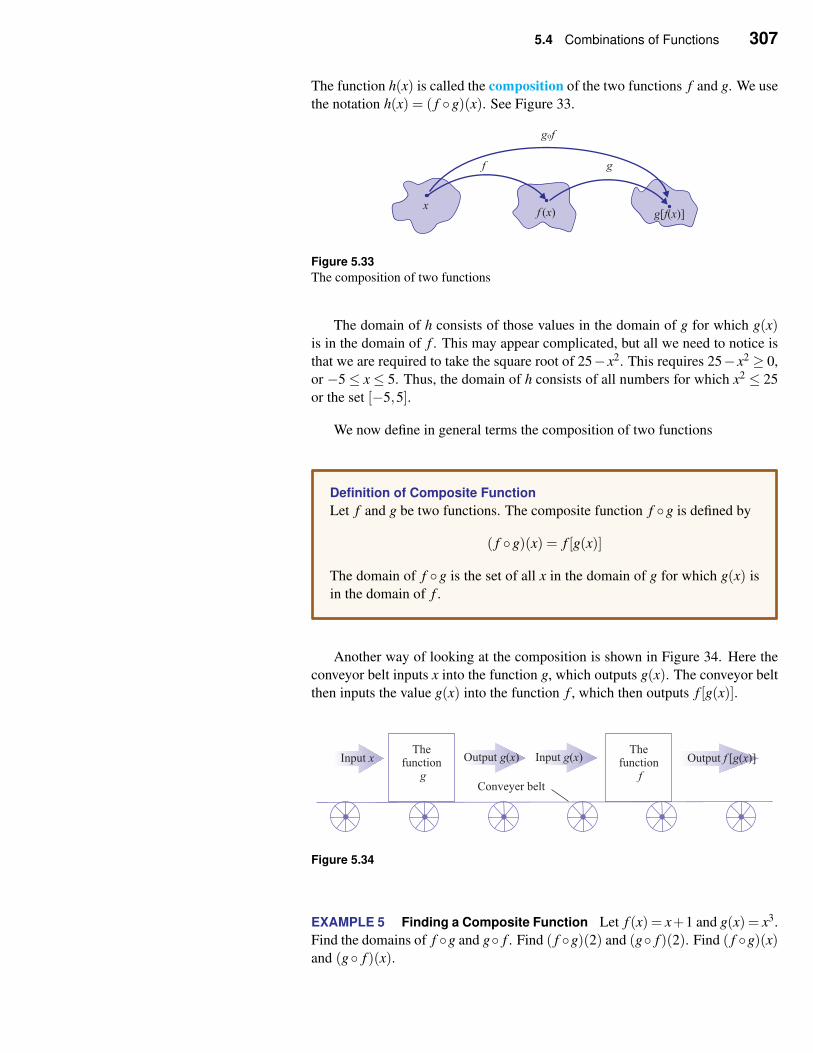
5.4 Combinations of Functions 307
The function h(x) is called the composition of the two functions f and g. We use
the notation h(x) = ( f ◦g)(x). See Figure 33.
f
xf x( )
g
g f x[ ( )]
g fo
Figure 5.33
The composition of two functions
The domain of h consists of those values in the domain of g for which g(x)is in the domain of f . This may appear complicated, but all we need to notice is
that we are required to take the square root of 25− x2. This requires 25− x2 ≥ 0,
or −5≤ x≤ 5. Thus, the domain of h consists of all numbers for which x2 ≤ 25
or the set [−5,5].
We now define in general terms the composition of two functions
Definition of Composite Function
Let f and g be two functions. The composite function f ◦g is defined by
( f ◦g)(x) = f [g(x)]
The domain of f ◦g is the set of all x in the domain of g for which g(x) is
in the domain of f .
Another way of looking at the composition is shown in Figure 34. Here the
conveyor belt inputs x into the function g, which outputs g(x). The conveyor belt
then inputs the value g(x) into the function f , which then outputs f [g(x)].
Thefunction
gConveyer belt
Input x Output ( )g x Input ( )g x Output [ ( )]f g xThe
functionf
Figure 5.34
EXAMPLE 5 Finding a Composite Function Let f (x) = x+1 and g(x) = x3.
Find the domains of f ◦g and g◦ f . Find ( f ◦g)(2) and (g◦ f )(2). Find ( f ◦g)(x)and (g◦ f )(x).
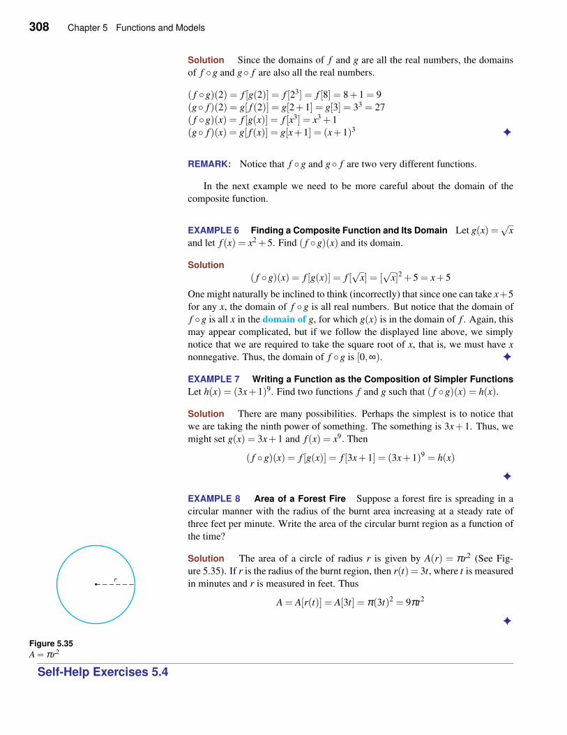
308 Chapter 5 Functions and Models
Solution Since the domains of f and g are all the real numbers, the domains
of f ◦g and g◦ f are also all the real numbers.
( f ◦g)(2) = f [g(2)] = f [23] = f [8] = 8+1 = 9
(g◦ f )(2) = g[ f (2)] = g[2+1] = g[3] = 33 = 27
( f ◦g)(x) = f [g(x)] = f [x3] = x3 +1
(g◦ f )(x) = g[ f (x)] = g[x+1] = (x+1)3 ✦
REMARK: Notice that f ◦g and g◦ f are two very different functions.
In the next example we need to be more careful about the domain of the
composite function.
EXAMPLE 6 Finding a Composite Function and Its Domain Let g(x) =√
x
and let f (x) = x2 +5. Find ( f ◦g)(x) and its domain.
Solution
( f ◦g)(x) = f [g(x)] = f [√
x] = [√
x]2 +5 = x+5
One might naturally be inclined to think (incorrectly) that since one can take x+5
for any x, the domain of f ◦ g is all real numbers. But notice that the domain of
f ◦g is all x in the domain of g, for which g(x) is in the domain of f . Again, this
may appear complicated, but if we follow the displayed line above, we simply
notice that we are required to take the square root of x, that is, we must have x
nonnegative. Thus, the domain of f ◦g is [0,∞). ✦
EXAMPLE 7 Writing a Function as the Composition of Simpler Functions
Let h(x) = (3x+1)9. Find two functions f and g such that ( f ◦g)(x) = h(x).
Solution There are many possibilities. Perhaps the simplest is to notice that
we are taking the ninth power of something. The something is 3x+1. Thus, we
might set g(x) = 3x+1 and f (x) = x9. Then
( f ◦g)(x) = f [g(x)] = f [3x+1] = (3x+1)9 = h(x)
✦
EXAMPLE 8 Area of a Forest Fire Suppose a forest fire is spreading in a
circular manner with the radius of the burnt area increasing at a steady rate of
three feet per minute. Write the area of the circular burnt region as a function of
the time?
Solution The area of a circle of radius r is given by A(r) = πr2 (See Fig-
ure 5.35). If r is the radius of the burnt region, then r(t) = 3t, where t is measured
in minutes and r is measured in feet. Thus
A = A[r(t)] = A[3t] = π(3t)2 = 9πt2
✦
r
�
Figure 5.35
A = πr2
Self-Help Exercises 5.4
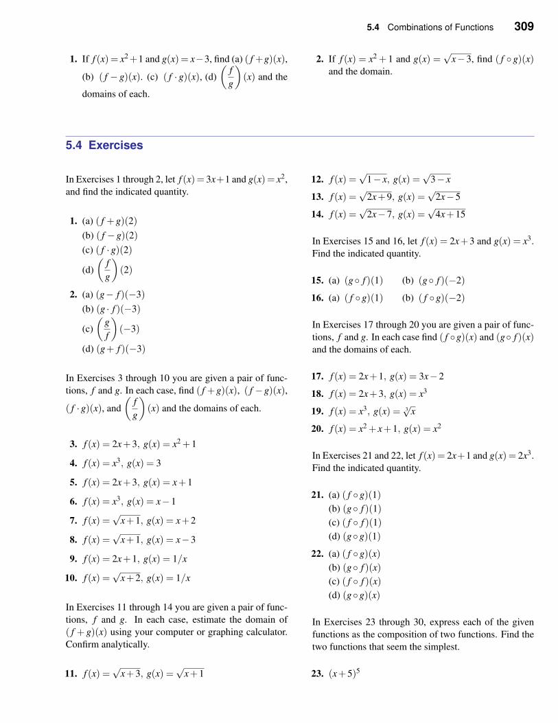
5.4 Combinations of Functions 309
1. If f (x) = x2+1 and g(x) = x−3, find (a) ( f +g)(x),
(b) ( f − g)(x). (c) ( f · g)(x), (d)
(f
g
)
(x) and the
domains of each.
2. If f (x) = x2 + 1 and g(x) =√
x−3, find ( f ◦ g)(x)and the domain.
5.4 Exercises
In Exercises 1 through 2, let f (x)= 3x+1 and g(x)= x2,
and find the indicated quantity.
1. (a) ( f +g)(2)
(b) ( f −g)(2)
(c) ( f ·g)(2)
(d)
(f
g
)
(2)
2. (a) (g− f )(−3)
(b) (g · f )(−3)
(c)
(g
f
)
(−3)
(d) (g+ f )(−3)
In Exercises 3 through 10 you are given a pair of func-
tions, f and g. In each case, find ( f +g)(x), ( f −g)(x),
( f ·g)(x), and
(f
g
)
(x) and the domains of each.
3. f (x) = 2x+3, g(x) = x2 +1
4. f (x) = x3, g(x) = 3
5. f (x) = 2x+3, g(x) = x+1
6. f (x) = x3, g(x) = x−1
7. f (x) =√
x+1, g(x) = x+2
8. f (x) =√
x+1, g(x) = x−3
9. f (x) = 2x+1, g(x) = 1/x
10. f (x) =√
x+2, g(x) = 1/x
In Exercises 11 through 14 you are given a pair of func-
tions, f and g. In each case, estimate the domain of
( f + g)(x) using your computer or graphing calculator.
Confirm analytically.
11. f (x) =√
x+3, g(x) =√
x+1
12. f (x) =√
1− x, g(x) =√
3− x
13. f (x) =√
2x+9, g(x) =√
2x−5
14. f (x) =√
2x−7, g(x) =√
4x+15
In Exercises 15 and 16, let f (x) = 2x+3 and g(x) = x3.
Find the indicated quantity.
15. (a) (g◦ f )(1) (b) (g◦ f )(−2)
16. (a) ( f ◦g)(1) (b) ( f ◦g)(−2)
In Exercises 17 through 20 you are given a pair of func-
tions, f and g. In each case find ( f ◦g)(x) and (g◦ f )(x)and the domains of each.
17. f (x) = 2x+1, g(x) = 3x−2
18. f (x) = 2x+3, g(x) = x3
19. f (x) = x3, g(x) = 3√
x
20. f (x) = x2 + x+1, g(x) = x2
In Exercises 21 and 22, let f (x) = 2x+1 and g(x) = 2x3.
Find the indicated quantity.
21. (a) ( f ◦g)(1)
(b) (g◦ f )(1)
(c) ( f ◦ f )(1)
(d) (g◦g)(1)
22. (a) ( f ◦g)(x)
(b) (g◦ f )(x)
(c) ( f ◦ f )(x)
(d) (g◦g)(x)
In Exercises 23 through 30, express each of the given
functions as the composition of two functions. Find the
two functions that seem the simplest.
23. (x+5)5
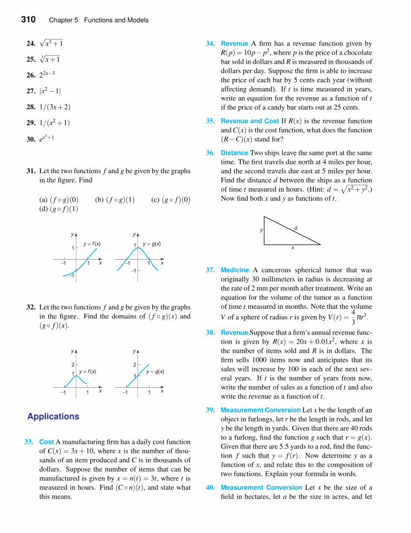
310 Chapter 5 Functions and Models
24.√
x3 +1
25. 3√
x+1
26. 22x−3
27. |x2−1|
28. 1/(3x+2)
29. 1/(x2 +1)
30. ex3+1
31. Let the two functions f and g be given by the graphs
in the figure. Find
(a) ( f ◦ g)(0) (b) ( f ◦ g)(1) (c) (g ◦ f )(0)(d) (g◦ f )(1)
32. Let the two functions f and g be given by the graphs
in the figure. Find the domains of ( f ◦ g)(x) and
(g◦ f )(x).
Applications
33. Cost A manufacturing firm has a daily cost function
of C(x) = 3x+ 10, where x is the number of thou-
sands of an item produced and C is in thousands of
dollars. Suppose the number of items that can be
manufactured is given by x = n(t) = 3t, where t is
measured in hours. Find (C ◦ n)(t), and state what
this means.
34. Revenue A firm has a revenue function given by
R(p) = 10p− p2, where p is the price of a chocolate
bar sold in dollars and R is measured in thousands of
dollars per day. Suppose the firm is able to increase
the price of each bar by 5 cents each year (without
affecting demand). If t is time measured in years,
write an equation for the revenue as a function of t
if the price of a candy bar starts out at 25 cents.
35. Revenue and Cost If R(x) is the revenue function
and C(x) is the cost function, what does the function
(R−C)(x) stand for?
36. Distance Two ships leave the same port at the same
time. The first travels due north at 4 miles per hour,
and the second travels due east at 5 miles per hour.
Find the distance d between the ships as a function
of time t measured in hours. (Hint: d =√
x2 + y2.)
Now find both x and y as functions of t.
37. Medicine A cancerous spherical tumor that was
originally 30 millimeters in radius is decreasing at
the rate of 2 mm per month after treatment. Write an
equation for the volume of the tumor as a function
of time t measured in months. Note that the volume
V of a sphere of radius r is given by V (r) =4
3πr3.
38. Revenue Suppose that a firm’s annual revenue func-
tion is given by R(x) = 20x + 0.01x2, where x is
the number of items sold and R is in dollars. The
firm sells 1000 items now and anticipates that its
sales will increase by 100 in each of the next sev-
eral years. If t is the number of years from now,
write the number of sales as a function of t and also
write the revenue as a function of t.
39. Measurement Conversion Let x be the length of an
object in furlongs, let r be the length in rods, and let
y be the length in yards. Given that there are 40 rods
to a furlong, find the function g such that r = g(x).Given that there are 5.5 yards to a rod, find the func-
tion f such that y = f (r). Now determine y as a
function of x, and relate this to the composition of
two functions. Explain your formula in words.
40. Measurement Conversion Let x be the size of a
field in hectares, let a be the size in acres, and let
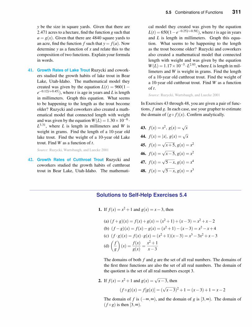
5.5 Combinations of Functions 311
y be the size in square yards. Given that there are
2.471 acres to a hectare, find the function g such that
a = g(x). Given that there are 4840 square yards to
an acre, find the function f such that y = f (a). Now
determine y as a function of x and relate this to the
composition of two functions. Explain your formula
in words.
41. Growth Rates of Lake Trout Ruzycki and cowork-
ers studied the growth habits of lake trout in Bear
Lake, Utah-Idaho. The mathematical model they
created was given by the equation L(t) = 960(1−e−0.12[t+0.45]), where t is age in years and L is length
in millimeters. Graph this equation. What seems
to be happening to the length as the trout become
older? Ruzycki and coworkers also created a math-
ematical model that connected length with weight
and was given by the equation W (L) = 1.30×10⁻⁶ ·L3.31, where L is length in millimeters and W is
weight in grams. Find the length of a 10-year old
lake trout. Find the weight of a 10-year old Lake
trout. Find W as a function of t.
Source: Ruzycki, Wurtsbaugh, and Luecke 2001
42. Growth Rates of Cutthroat Trout Ruzycki and
coworkers studied the growth habits of cuttthroat
trout in Bear Lake, Utah-Idaho. The mathemati-
cal model they created was given by the equation
L(t) = 650(1−e−0.25[t+0.50]), where t is age in years
and L is length in millimeters. Graph this equa-
tion. What seems to be happening to the length
as the trout become older? Ruzycki and coworkers
also created a mathematical model that connected
length with weight and was given by the equation
W (L) = 1.17×10⁻⁵ ·L2.93, where L is length in mil-
limeters and W is weight in grams. Find the length
of a 10-year old cutthroat trout. Find the weight of
a 10-year old cutthroat trout. Find W as a function
of t.
Source: Ruzycki, Wurtsbaugh, and Luecke 2001
In Exercises 43 through 48, you are given a pair of func-
tions, f and g. In each case, use your grapher to estimate
the domain of (g◦ f )(x). Confirm analytically.
43. f (x) = x2, g(x) =√
x
44. f (x) = |x|, g(x) =√
x
45. f (x) =√
x+5, g(x) = x2
46. f (x) =√
x−5, g(x) = x2
47. f (x) =√
5− x, g(x) = x4
48. f (x) =√
5− x, g(x) = x3
Solutions to Self-Help Exercises 5.4
1. If f (x) = x2 +1 and g(x) = x−3, then
(a) ( f +g)(x) = f (x)+g(x) = (x2 +1)+(x−3) = x2 + x−2
(b) ( f −g)(x) = f (x)−g(x) = (x2 +1)− (x−3) = x2− x+4
(c) ( f ·g)(x) = f (x) ·g(x) = (x2 +1)(x−3) = x3−3x2 + x−3
(d)
(f
g
)
(x) =f (x)
g(x)=
x2 +1
x−3
The domains of both f and g are the set of all real numbers. The domains of
the first three functions are also the set of all real numbers. The domain of
the quotient is the set of all real numbers except 3.
2. If f (x) = x2 +1 and g(x) =√
x−3, then
( f ◦g)(x) = f [g(x)] = (√
x−3)2 +1 = (x−3)+1 = x−2
The domain of f is (−∞,∞), and the domain of g is [3,∞). The domain of
( f ◦g) is then [3,∞).
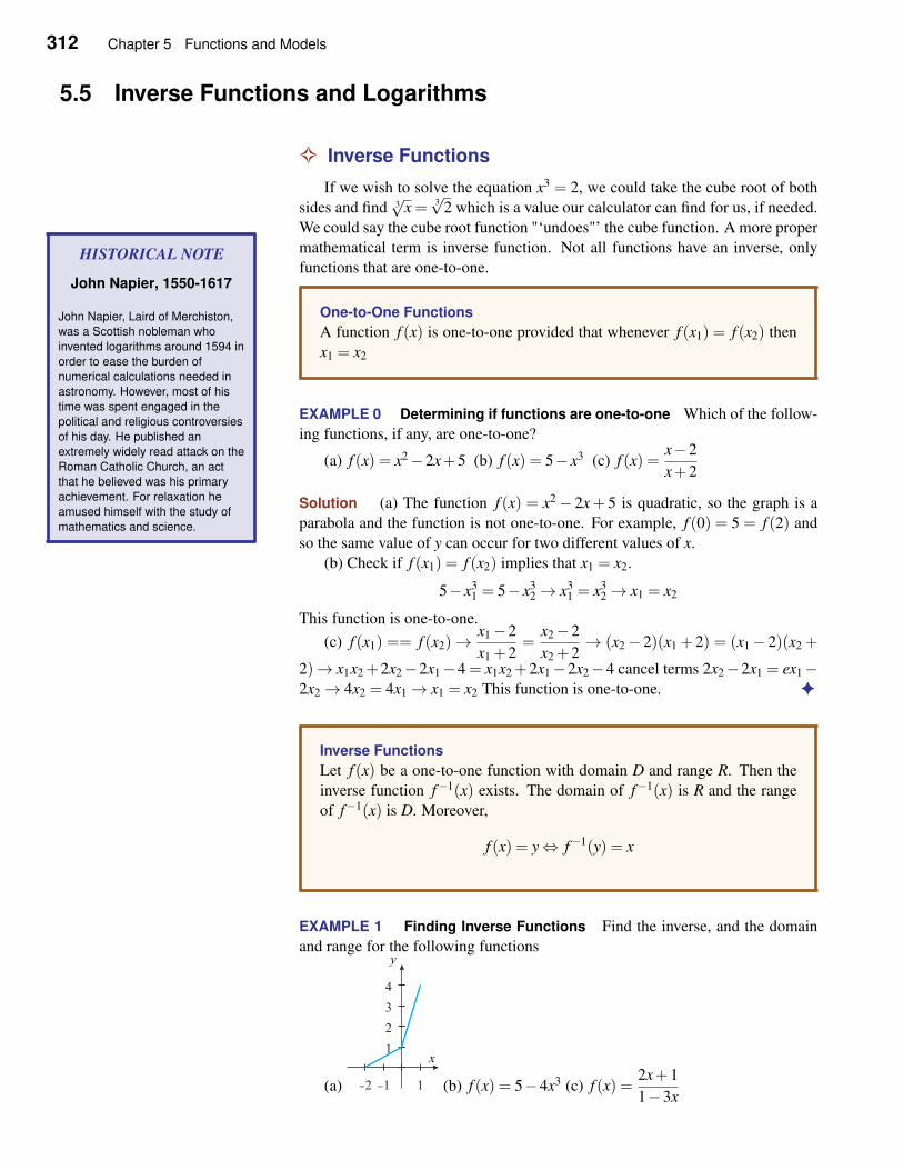
312 Chapter 5 Functions and Models
5.5 Inverse Functions and Logarithms
✧ Inverse Functions
If we wish to solve the equation x3 = 2, we could take the cube root of both
sides and find 3√
x = 3√
2 which is a value our calculator can find for us, if needed.
We could say the cube root function "‘undoes"’ the cube function. A more proper
mathematical term is inverse function. Not all functions have an inverse, only
functions that are one-to-one.
One-to-One Functions
A function f (x) is one-to-one provided that whenever f (x1) = f (x2) then
x1 = x2
HISTORICAL NOTE
John Napier, 1550-1617
John Napier, Laird of Merchiston,
was a Scottish nobleman who
invented logarithms around 1594 in
order to ease the burden of
numerical calculations needed in
astronomy. However, most of his
time was spent engaged in the
political and religious controversies
of his day. He published an
extremely widely read attack on the
Roman Catholic Church, an act
that he believed was his primary
achievement. For relaxation he
amused himself with the study of
mathematics and science.
EXAMPLE 0 Determining if functions are one-to-one Which of the follow-
ing functions, if any, are one-to-one?
(a) f (x) = x2−2x+5 (b) f (x) = 5− x3 (c) f (x) =x−2
x+2
Solution (a) The function f (x) = x2− 2x+ 5 is quadratic, so the graph is a
parabola and the function is not one-to-one. For example, f (0) = 5 = f (2) and
so the same value of y can occur for two different values of x.
(b) Check if f (x1) = f (x2) implies that x1 = x2.
5− x31 = 5− x3
2→ x31 = x3
2→ x1 = x2
This function is one-to-one.
(c) f (x1) == f (x2)→x1−2
x1 +2=
x2−2
x2 +2→ (x2− 2)(x1 + 2) = (x1− 2)(x2 +
2)→ x1x2 +2x2−2x1−4 = x1x2 +2x1−2x2−4 cancel terms 2x2−2x1 = ex1−2x2→ 4x2 = 4x1→ x1 = x2 This function is one-to-one. ✦
Inverse Functions
Let f (x) be a one-to-one function with domain D and range R. Then the
inverse function f−1(x) exists. The domain of f−1(x) is R and the range
of f−1(x) is D. Moreover,
f (x) = y⇔ f−1(y) = x
EXAMPLE 1 Finding Inverse Functions Find the inverse, and the domain
and range for the following functions
(a)
x
y
-2 -1 1
1
2
3
4
(b) f (x) = 5−4x3 (c) f (x) =2x+1
1−3x
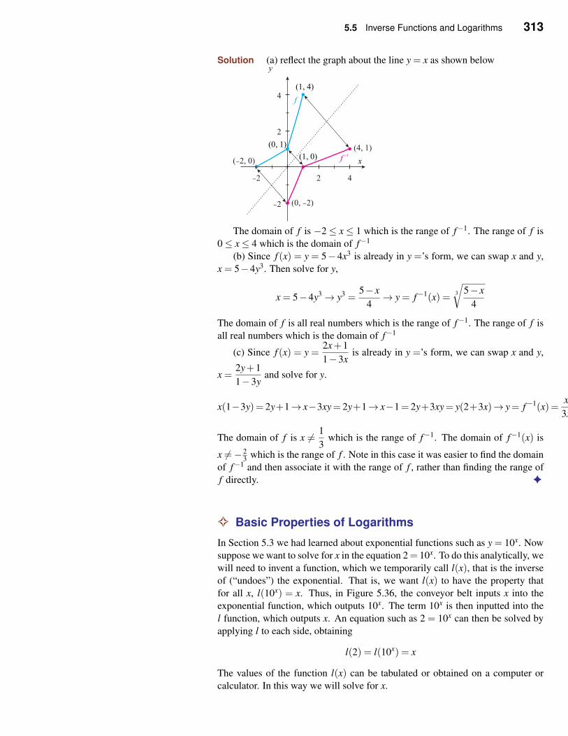
5.5 Inverse Functions and Logarithms 313
Solution (a) reflect the graph about the line y = x as shown below
x
y
(0, 1)
(1, 0)
-2 2 4
-2
2
4
(0, 2)-
(1, 4)
(4, 1)
f
f-1
( 2, 0)-
The domain of f is −2≤ x≤ 1 which is the range of f−1. The range of f is
0≤ x≤ 4 which is the domain of f−1
(b) Since f (x) = y = 5− 4x3 is already in y =’s form, we can swap x and y,
x = 5−4y3. Then solve for y,
x = 5−4y3→ y3 =5− x
4→ y = f−1(x) =
3
√
5− x
4
The domain of f is all real numbers which is the range of f−1. The range of f is
all real numbers which is the domain of f−1
(c) Since f (x) = y =2x+1
1−3xis already in y =’s form, we can swap x and y,
x =2y+1
1−3yand solve for y.
x(1−3y)= 2y+1→ x−3xy= 2y+1→ x−1= 2y+3xy= y(2+3x)→ y= f−1(x)=x
3x
The domain of f is x 6= 1
3which is the range of f−1. The domain of f−1(x) is
x 6=− 23 which is the range of f . Note in this case it was easier to find the domain
of f−1 and then associate it with the range of f , rather than finding the range of
f directly. ✦
✧ Basic Properties of Logarithms
In Section 5.3 we had learned about exponential functions such as y = 10x. Now
suppose we want to solve for x in the equation 2= 10x. To do this analytically, we
will need to invent a function, which we temporarily call l(x), that is the inverse
of (“undoes”) the exponential. That is, we want l(x) to have the property that
for all x, l(10x) = x. Thus, in Figure 5.36, the conveyor belt inputs x into the
exponential function, which outputs 10x. The term 10x is then inputted into the
l function, which outputs x. An equation such as 2 = 10x can then be solved by
applying l to each side, obtaining
l(2) = l(10x) = x
The values of the function l(x) can be tabulated or obtained on a computer or
calculator. In this way we will solve for x.
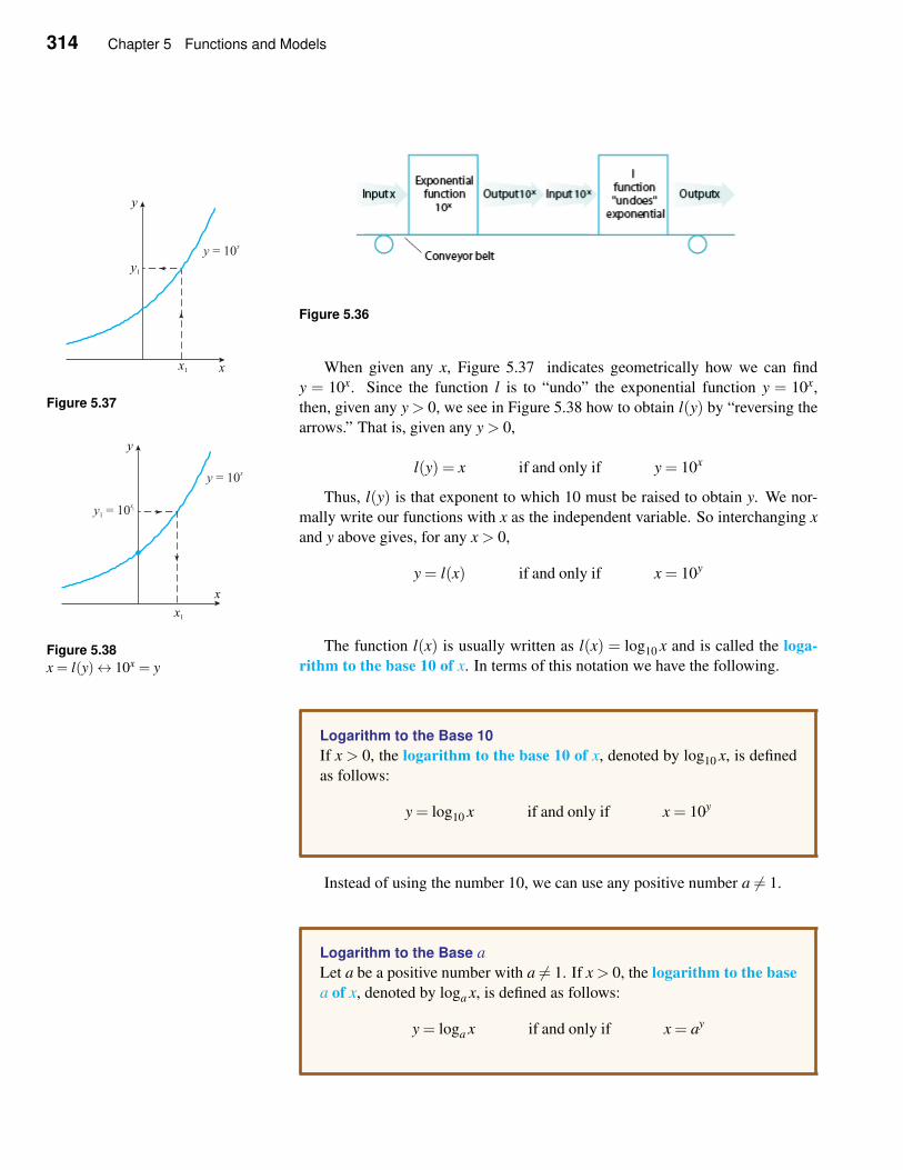
314 Chapter 5 Functions and Models
Figure 5.36
When given any x, Figure 5.37 indicates geometrically how we can findx1 x
y
y = 10x
y1
Figure 5.37y = 10x. Since the function l is to “undo” the exponential function y = 10x,
then, given any y > 0, we see in Figure 5.38 how to obtain l(y) by “reversing the
arrows.” That is, given any y > 0,
l(y) = x if and only if y = 10x
Thus, l(y) is that exponent to which 10 must be raised to obtain y. We nor-
mally write our functions with x as the independent variable. So interchanging x
and y above gives, for any x > 0,
y = l(x) if and only if x = 10y
x1
x
y
y = 10x
y1 = 10x1
Figure 5.38
x = l(y)↔ 10x = y
The function l(x) is usually written as l(x) = log10 x and is called the loga-
rithm to the base 10 of x. In terms of this notation we have the following.
Logarithm to the Base 10
If x > 0, the logarithm to the base 10 of x, denoted by log10 x, is defined
as follows:
y = log10 x if and only if x = 10y
Instead of using the number 10, we can use any positive number a 6= 1.
Logarithm to the Base a
Let a be a positive number with a 6= 1. If x > 0, the logarithm to the base
a of x, denoted by loga x, is defined as follows:
y = loga x if and only if x = ay
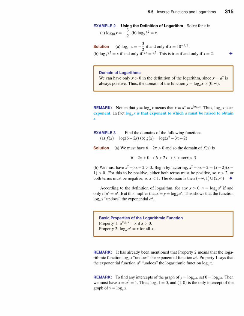
5.5 Inverse Functions and Logarithms 315
EXAMPLE 2 Using the Definition of Logarithm Solve for x in
(a) log10 x =−3
2, (b) log3 32 = x.
Solution (a) log10 x =−3
2if and only if x = 10−3/2.
(b) log3 32 = x if and only if 3x = 32. This is true if and only if x = 2. ✦
Domain of Logarithms
We can have only x > 0 in the definition of the logarithm, since x = ay is
always positive. Thus, the domain of the function y = loga x is (0,∞).
REMARK: Notice that y = loga x means that x = ay = aloga x. Thus, loga x is an
exponent. In fact loga x is that exponent to which a must be raised to obtain
x.
EXAMPLE 3 Find the domains of the following functions
(a) f (x) = log(6−2x) (b) g(x) = log(x2−3x+2)
Solution (a) We must have 6−2x > 0 and so the domain of f (x) is
6−2x > 0→ 6 > 2x→ 3 > xorx < 3
(b) We must have x2−3x+2 > 0. Begin by factoring, x2−3x+2 = (x−2)(x−1) > 0. For this to be positive, either both terms must be positive, so x > 2, or
both terms must be negative, so x < 1. The domain is then (−∞,1)∪ (2,∞) ✦
According to the definition of logarithm, for any x > 0, y = loga ax if and
only if ax = ay. But this implies that x = y = loga ax. This shows that the function
loga x “undoes” the exponential ax.
Basic Properties of the Logarithmic Function
Property 1. aloga x = x if x > 0.
Property 2. loga ax = x for all x.
REMARK: It has already been mentioned that Property 2 means that the loga-
rithmic function loga x “undoes” the exponential function ax. Property 1 says that
the exponential function ax “undoes” the logarithmic function loga x.
REMARK: To find any intercepts of the graph of y = loga x, set 0 = loga x. Then
we must have x = a0 = 1. Thus, loga 1 = 0, and (1,0) is the only intercept of the
graph of y = loga x.
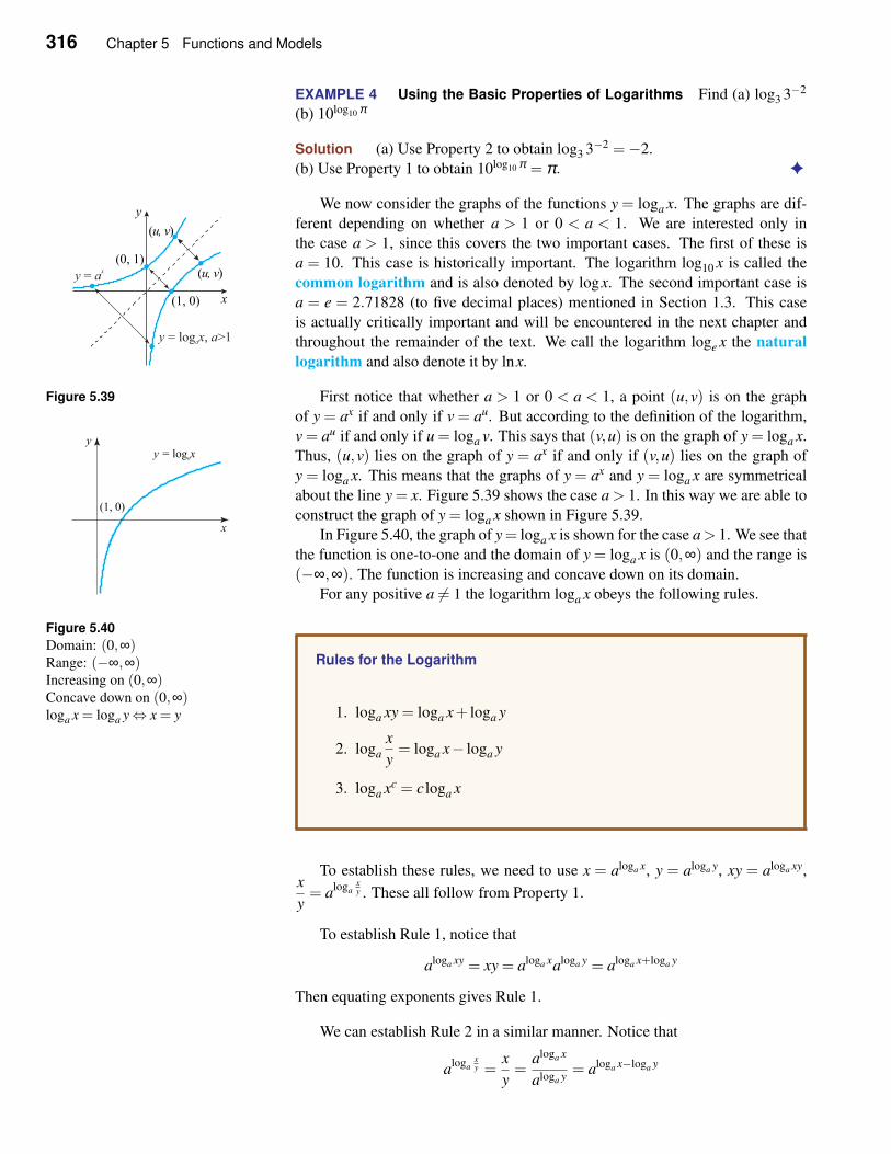
316 Chapter 5 Functions and Models
EXAMPLE 4 Using the Basic Properties of Logarithms Find (a) log3 3−2
(b) 10log10 π
Solution (a) Use Property 2 to obtain log3 3−2 =−2.
(b) Use Property 1 to obtain 10log10 π = π. ✦
We now consider the graphs of the functions y = loga x. The graphs are dif-
ferent depending on whether a > 1 or 0 < a < 1. We are interested only in
the case a > 1, since this covers the two important cases. The first of these is
a = 10. This case is historically important. The logarithm log10 x is called the
common logarithm and is also denoted by logx. The second important case is
a = e = 2.71828 (to five decimal places) mentioned in Section 1.3. This case
is actually critically important and will be encountered in the next chapter and
throughout the remainder of the text. We call the logarithm loge x the natural
logarithm and also denote it by lnx.
x
y
(0, 1)
(u, v)
(u, v)
(1, 0)
y x a= log , >1a
y a= x
Figure 5.39 First notice that whether a > 1 or 0 < a < 1, a point (u,v) is on the graph
of y = ax if and only if v = au. But according to the definition of the logarithm,
v = au if and only if u = loga v. This says that (v,u) is on the graph of y = loga x.
Thus, (u,v) lies on the graph of y = ax if and only if (v,u) lies on the graph of
y = loga x. This means that the graphs of y = ax and y = loga x are symmetrical
about the line y = x. Figure 5.39 shows the case a > 1. In this way we are able to
construct the graph of y = loga x shown in Figure 5.39.
In Figure 5.40, the graph of y= loga x is shown for the case a> 1. We see that
the function is one-to-one and the domain of y = loga x is (0,∞) and the range is
(−∞,∞). The function is increasing and concave down on its domain.
x
y
(1, 0)
��
�
� �
y = xloga
Figure 5.40
Domain: (0,∞)Range: (−∞,∞)Increasing on (0,∞)Concave down on (0,∞)loga x = loga y⇔ x = y
For any positive a 6= 1 the logarithm loga x obeys the following rules.
Rules for the Logarithm
1. loga xy = loga x+ loga y
2. loga
x
y= loga x− loga y
3. loga xc = c loga x
To establish these rules, we need to use x = aloga x, y = aloga y, xy = aloga xy,x
y= a
logaxy . These all follow from Property 1.
To establish Rule 1, notice that
aloga xy = xy = aloga xaloga y = aloga x+loga y
Then equating exponents gives Rule 1.
We can establish Rule 2 in a similar manner. Notice that
aloga
xy =
x
y=
aloga x
aloga y= aloga x−loga y
5.5 Inverse Functions and Logarithms 317
Equating exponents gives Rule 2.
To establish Rule 3, notice that
aloga xc
= xc =(aloga x
)c= ac loga x
Equating exponents gives Rule 3.
✧ Solving Equations with Exponents and Logarithms
If we wish to solve an equation with a logarithm, then at an appropriate point
in the calculation we can use the definition of logarithm, as in the following
example.
EXAMPLE 5 Solving an Equation with a Logarithm Solve 2log(2x+5)+6 = 0.
Solution
2log(2x+5)+6 = 0
log(2x+5) = −3
2x+5 = 10−3 = 0.001 definition of logarithm
x =1
2(−4.999) =−2.4995
✦
REMARK: In the example above, we had log(2x+ 5) = −3 at one point. We
could have applied the exponential function to each side of this equation to
“undo” the logarithm. Thus,
10−3 = 10log(2x+5) = 2x+5
by Property 1.
✧ More on the Natural Logarithm
We summarize here the definition of natural logarithm.
Natural Logarithm
If x > 0, the natural logarithm of x, denoted by lnx, is defined as follows:
y = lnx if and only if x = ey
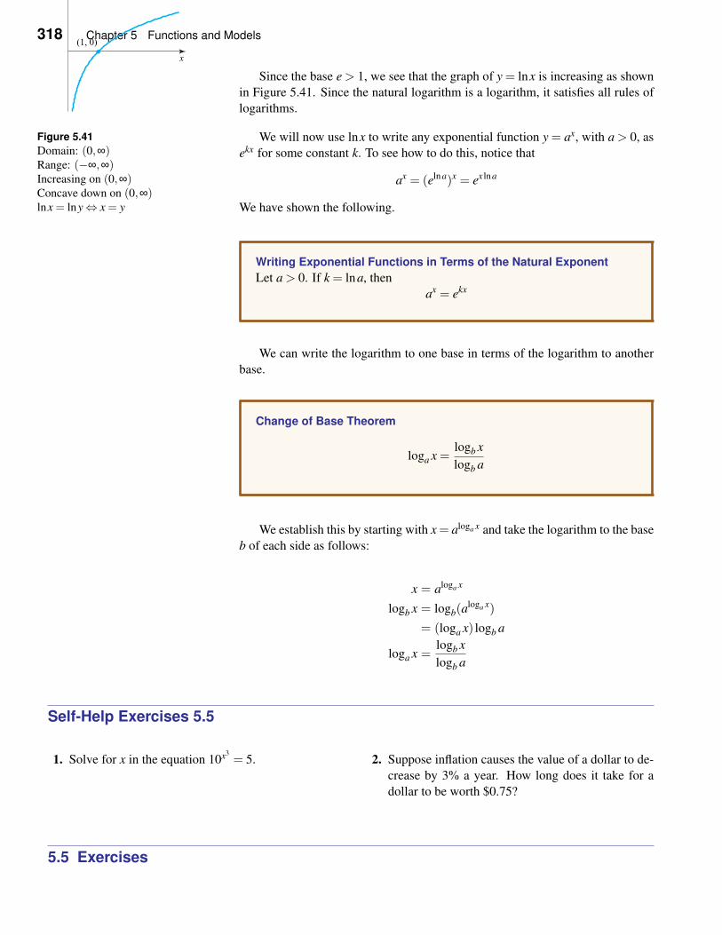
318 Chapter 5 Functions and Models
Since the base e > 1, we see that the graph of y = lnx is increasing as shown
in Figure 5.41. Since the natural logarithm is a logarithm, it satisfies all rules of
logarithms.
x
y
(1, 0)
� �
y x= ln
Figure 5.41
Domain: (0,∞)Range: (−∞,∞)Increasing on (0,∞)Concave down on (0,∞)lnx = lny⇔ x = y
We will now use lnx to write any exponential function y = ax, with a > 0, as
ekx for some constant k. To see how to do this, notice that
ax = (elna)x = ex lna
We have shown the following.
Writing Exponential Functions in Terms of the Natural Exponent
Let a > 0. If k = lna, then
ax = ekx
We can write the logarithm to one base in terms of the logarithm to another
base.
Change of Base Theorem
loga x =logb x
logb a
We establish this by starting with x = aloga x and take the logarithm to the base
b of each side as follows:
x = aloga x
logb x = logb(aloga x)
= (loga x) logb a
loga x =logb x
logb a
Self-Help Exercises 5.5
1. Solve for x in the equation 10x3= 5. 2. Suppose inflation causes the value of a dollar to de-
crease by 3% a year. How long does it take for a
dollar to be worth $0.75?
5.5 Exercises

5.5 Inverse Functions and Logarithms 319
In Exercises 1 through 6, solve for x.
1. logx = 2
2. logx =−3
3. lnx =−π
4. lnx =−3
4
5. 3log3 x = 5
6. 2log2 x = 9
In Exercises 7 through 16, simplify.
7. log104
8. log√
10
9. log1
10
10. log1√10
11. 10log2π
12. 10log√
2
13. e3ln2
14. e0.5ln9
15.(5log5 3
)4
16.√
3log3 2
In Exercises 17 through 22, write the given quantity in
terms of logx, logy, and logz.
17. logx2√yz
18. log√
xyz
19. log
√xy
z
20. logxy2
z3
21. log
√xy
z
22. logx2y3
√z
In Exercises 23 through 28, write the given quantity as
one logarithm.
23. 2logx+ logy
24. 2logx− logy
25. 12 logx− 1
3 logy
26. 2logx− 12
logy+ logz
27. 3lnx+ lny− 13 lnz
28.√
2lnx− lny
In Exercises 29 through 40, solve the equation for x.
29. 5 ·105x = 3
30. 2 ·103x = 5
31. 6 = 2 ·10−2x
32. 3 = 4 ·10−0.5x
33. 2 ·103x−1 = 1
34. 3 ·102−5x = 4
35. ex2= 4
36. e√
x = 4
37. 2log(x+7)+3 = 0
38. logx2 = 9
39. log(log4x) = 0
40. log3x = log6
In Exercises 41 through 43, use basic graphing princi-
ples to sketch the graphs. Then support your answers,
using a grapher.
41. y = logx, y = log(x+3), y = log(x−3)
42. y = logx, y = 2logx, y = 0.25logx
43. y = logx, y =− logx
44. Solve the equation 10x = − logx approximately on
your computer or graphing calculator.
45. On your computer or graphing calculator, find all
solutions to logx = x2−2.
46. Write 2x as ekx for some k.
47. Write 10x as ekx for some k.
Applications
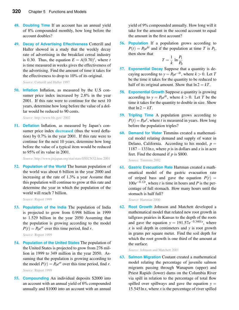
320 Chapter 5 Functions and Models
48. Doubling Time If an account has an annual yield
of 8% compounded monthly, how long before the
account doubles?
49. Decay of Advertising Effectiveness Cotterill and
Haller showed in a study that the weekly decay
rate of advertising in the breakfast cereal industry
is 0.30. Thus, the equation E = A(0.70)t , where t
is time measured in weeks gives the effectiveness of
the advertising. Find the amount of time it takes for
the effectiveness to drop to 10% of its original.
Source: Cotterill and Haller 1997
50. Inflation Inflation, as measured by the U.S con-
sumer price index increased by 2.8% in the year
2001. If this rate were to continue for the next 10
years, determine how long before the value of a dol-
lar would be reduced to 90 cents.
Source: http://www.bls.gov/ 2002
51. Deflation Inflation, as measured by Japan’s con-
sumer price index decreased (thus the word defla-
tion) by 0.7% in the year 2001. If this rate were to
continue for the next 10 years, determine how long
before the value of a typical item would be reduced
to 95% of its value in 2001.
Source: http://www.jinjapan.org/stat/stats/05ECN32.htm 2001
52. Population of the World The human population of
the world was about 6 billion in the year 2000 and
increasing at the rate of 1.3% a year Assume that
this population will continue to grow at this rate and
determine the year in which the population of the
world will reach 7 billion.
Source: Report 1999
53. Population of the India The population of India
is projected to grow from 0.998 billion in 1999
to 1.529 billion in the year 2050 Assuming that
the population is growing according to the model
P(t) = P0ert over this time period, find r.
Source: Report 1999
54. Population of the United States The population of
the United States is projected to grow from 276 mil-
lion in 1999 to 349 million in the year 2050. As-
suming that the population is growing according to
the model P(t) = P0ert over this time period, find r.
Source: Report 1999
55. Compounding An individual deposits $2000 into
an account with an annual yield of 6% compounded
annually and $1000 into an account with an annual
yield of 9% compounded annually. How long will it
take for the amount in the second account to equal
the amount in the first account?
56. Population If a population grows according to
P(t) = P0ekt and if the population at time T is P1,
then show that
T =1
kln
P1
P0
57. Exponential Decay Suppose that a quantity is de-
caying according to y = P0e−kt , where k > 0. Let T
be the time it takes for the quantity to be reduced to
half of its original amount. Show that ln2 = kT .
58. Exponential Growth Suppose a quantity is growing
according to y = P0ekt , where k > 0. Let T be the
time it takes for the quantity to double in size. Show
that ln2 = kT .
59. Tripling Time A population grows according to
P(t) = P0et , where t is measured in years. How long
before the population triples?
60. Demand for Water Timmins created a mathemati-
cal model relating demand and supply of water in
Delano, California. According to his model, p =1187−133lnx, where p is in dollars and x is in acre
feet. Find the demand if p is $800.
Source: Timmins 2002
61. Gastric Evacuation Rate Hartman created a math-
ematical model of the gastric evacuation rate
of striped bass and gave the equation P(t) =100e−0.12t , where t is time in hours and P is the per-
centage of full stomach. How many hours until the
stomach is half full?
Source: Hartman 2000
62. Root Growth Johnson and Matchett developed a
mathematical model that related new root growth in
tallgrass prairies in Kansas to the depth of the roots
and gave the equation y = 191.57e−0.3401x, where
x is soil depth in centimeters and y is root growth
in grams per square meter. Find the soil depth for
which the root growth is one third of the amount at
the surface.
Source: Johnson and Matchett 2001
63. Salmon Migration Coutant created a mathematical
model relating the percentage of juvenile salmon
migrants passing through Wanapum (upper) and
Priest Rapids (lower) dams on the Columbia River
via spill in relation to the percentage of total flow
spilled over spillways and gave the equation y =15.545lnx, where x is the percentage of river spilled
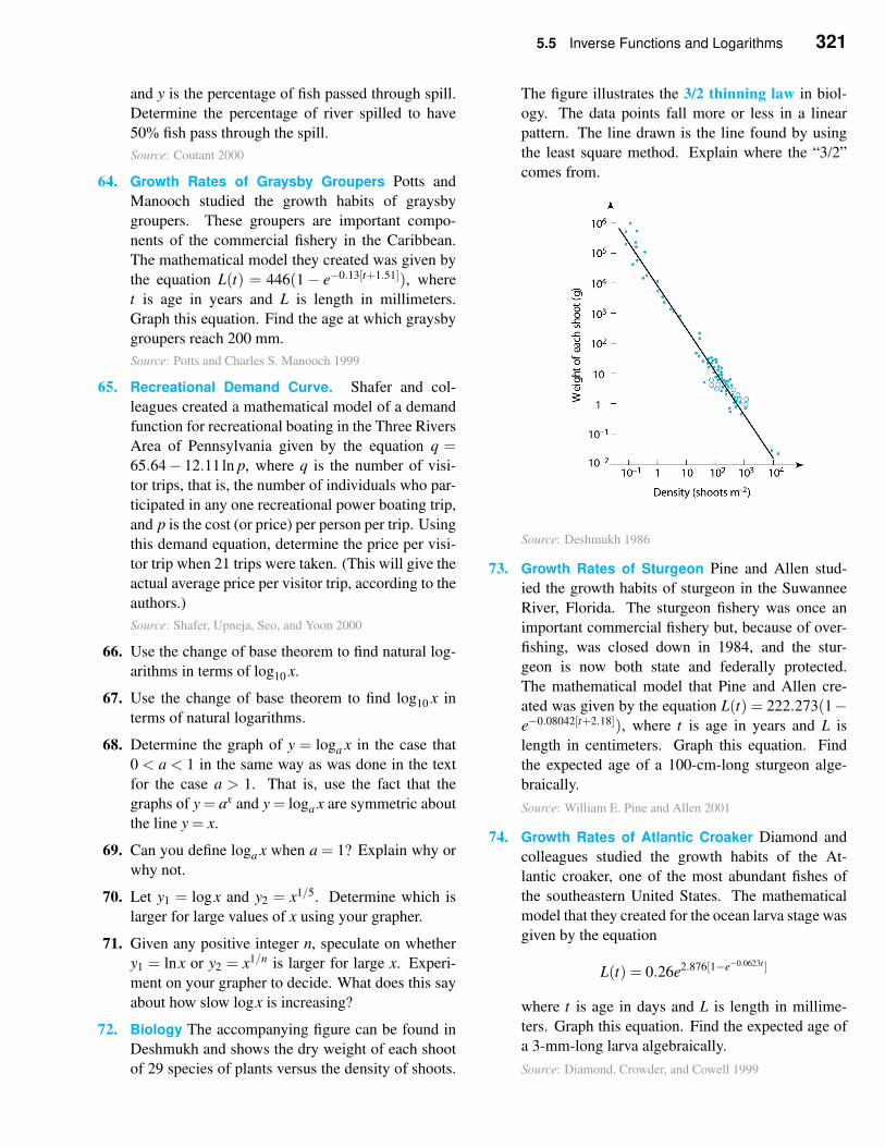
5.5 Inverse Functions and Logarithms 321
and y is the percentage of fish passed through spill.
Determine the percentage of river spilled to have
50% fish pass through the spill.
Source: Coutant 2000
64. Growth Rates of Graysby Groupers Potts and
Manooch studied the growth habits of graysby
groupers. These groupers are important compo-
nents of the commercial fishery in the Caribbean.
The mathematical model they created was given by
the equation L(t) = 446(1− e−0.13[t+1.51]), where
t is age in years and L is length in millimeters.
Graph this equation. Find the age at which graysby
groupers reach 200 mm.
Source: Potts and Charles S. Manooch 1999
65. Recreational Demand Curve. Shafer and col-
leagues created a mathematical model of a demand
function for recreational boating in the Three Rivers
Area of Pennsylvania given by the equation q =65.64− 12.11ln p, where q is the number of visi-
tor trips, that is, the number of individuals who par-
ticipated in any one recreational power boating trip,
and p is the cost (or price) per person per trip. Using
this demand equation, determine the price per visi-
tor trip when 21 trips were taken. (This will give the
actual average price per visitor trip, according to the
authors.)
Source: Shafer, Upneja, Seo, and Yoon 2000
66. Use the change of base theorem to find natural log-
arithms in terms of log10 x.
67. Use the change of base theorem to find log10 x in
terms of natural logarithms.
68. Determine the graph of y = loga x in the case that
0 < a < 1 in the same way as was done in the text
for the case a > 1. That is, use the fact that the
graphs of y = ax and y = loga x are symmetric about
the line y = x.
69. Can you define loga x when a = 1? Explain why or
why not.
70. Let y1 = logx and y2 = x1/5. Determine which is
larger for large values of x using your grapher.
71. Given any positive integer n, speculate on whether
y1 = lnx or y2 = x1/n is larger for large x. Experi-
ment on your grapher to decide. What does this say
about how slow logx is increasing?
72. Biology The accompanying figure can be found in
Deshmukh and shows the dry weight of each shoot
of 29 species of plants versus the density of shoots.
The figure illustrates the 3/2 thinning law in biol-
ogy. The data points fall more or less in a linear
pattern. The line drawn is the line found by using
the least square method. Explain where the “3/2”
comes from.
Source: Deshmukh 1986
73. Growth Rates of Sturgeon Pine and Allen stud-
ied the growth habits of sturgeon in the Suwannee
River, Florida. The sturgeon fishery was once an
important commercial fishery but, because of over-
fishing, was closed down in 1984, and the stur-
geon is now both state and federally protected.
The mathematical model that Pine and Allen cre-
ated was given by the equation L(t) = 222.273(1−e−0.08042[t+2.18]), where t is age in years and L is
length in centimeters. Graph this equation. Find
the expected age of a 100-cm-long sturgeon alge-
braically.
Source: William E. Pine and Allen 2001
74. Growth Rates of Atlantic Croaker Diamond and
colleagues studied the growth habits of the At-
lantic croaker, one of the most abundant fishes of
the southeastern United States. The mathematical
model that they created for the ocean larva stage was
given by the equation
L(t) = 0.26e2.876[1−e−0.0623t ]
where t is age in days and L is length in millime-
ters. Graph this equation. Find the expected age of
a 3-mm-long larva algebraically.
Source: Diamond, Crowder, and Cowell 1999
Solutions to Self-Help Exercises 5.5
1. Taking the logarithm of each side gives
log5 = log10x3
= x3
Thus x = 3√
log5 = 3√
0.69897≈ 0.88747.
2. The value V (t) of the dollar is V (t) = (0.97)t , where t is given in years. We
must find t so that 0.75 =V (t) = (0.97)t . We have
0.75 = (0.97)t
log0.75 = log(0.97)t
= t log0.97
t =log0.75
log0.97≈ 9.4
Thus, at this rate a dollar will be reduced in value to $0.75 in about 9.4 years.
5.6 Review
✧ Summary Outline
• A function f from the set D to the set R is a rule that assigns to each
element x in D one and only one element y = f (x) in R.
• The set D above is called the domain.
• One thinks of the domain as the set of inputs and the values y = f (x) as the
outputs.
• The set of all possible outputs is called the range.
• The letter representing the elements in the domain is called the indepen-
dent variable.
• The letter representing the elements in the range is called the dependent
variable.
• The graph of the function f consists of all points (x,y) such that x is in the
domain of f and y = f (x).
• A function is increasing (ր) on the interval (a,b) if the values of f (x)increase as x increases. A function is decreasing (ւ) on the interval (a,b)if the values of f (x) decrease as x increases.
322
Chapter 5 Review 323
• A function is concave up (⌣) on the interval (a,b) if the graph is bent
upward there. A function is concave down (⌢) on the interval (a,b) if the
graph is bent downward there.
• Vertical line test. A graph in the xy-plane represents a function, if and
only if that every vertical line intersects the graph in at most one place.
• The function f (x) = ax2 +bx+ c, a 6= 0 is called a quadratic function.
• Every quadratic function f (x) = ax2 + bx + c with a 6= 0 can be put in
standard form f (x) = a(x−h)2+k by completing the square. The point
(h,k) is called the vertex.
• When a < 0, the graph of the quadratic y = ax2 +bx+ c looks like ⌢ and
assumes the maximum value k when x = h.
• When a > 0, the graph of the quadratic y = ax2 +bx+ c looks like ⌣ and
assumes the minimum value k when x = h.
• An exponential function is a function of the form y = ax.
• Properties of ax.
a > 1 0 < a < 1
increasing on (−∞,∞) decreasing on (−∞,∞)
domain = (−∞,∞)
range = (0,∞)
ax = ay if and only if x = y
• Logarithm to Base a. Let a be a positive number with a 6= 1. If x > 0, the
logarithm to the base a of x, denoted by loga x, is defined as y = loga x if
and only if x = ay.
• Properties of Logarithms
aloga x = x if x > 0 loga ax = x for all x
loga 1 = 0 loga xy = loga x+ loga y
loga
x
y= loga x− loga y loga xc = c loga x
• The number e to five decimals is 2.71828.
• Natural Logarithm. If x > 0, the natural logarithm of x, denoted by lnx,
is defined as y = lnx if, and only if, x = ey.
• For any a > 0, ax = ekx if k = lna.
• If a quantity grows according to Q(t) = Q0(1+ k)t or according to Q(t) =Q0ekt , where k > 0, k is called the growth constant.
• If a quantity decays according to Q(t) = Q0(1−k)t or according to Q(t) =Q0ekt , where k > 0, k is called the decay constant.
• The half-life of a radioactive substance is the time that must elapse for half
of the material to decay.
• The sum f +g is defined by ( f +g)(x) = f (x)+g(x).
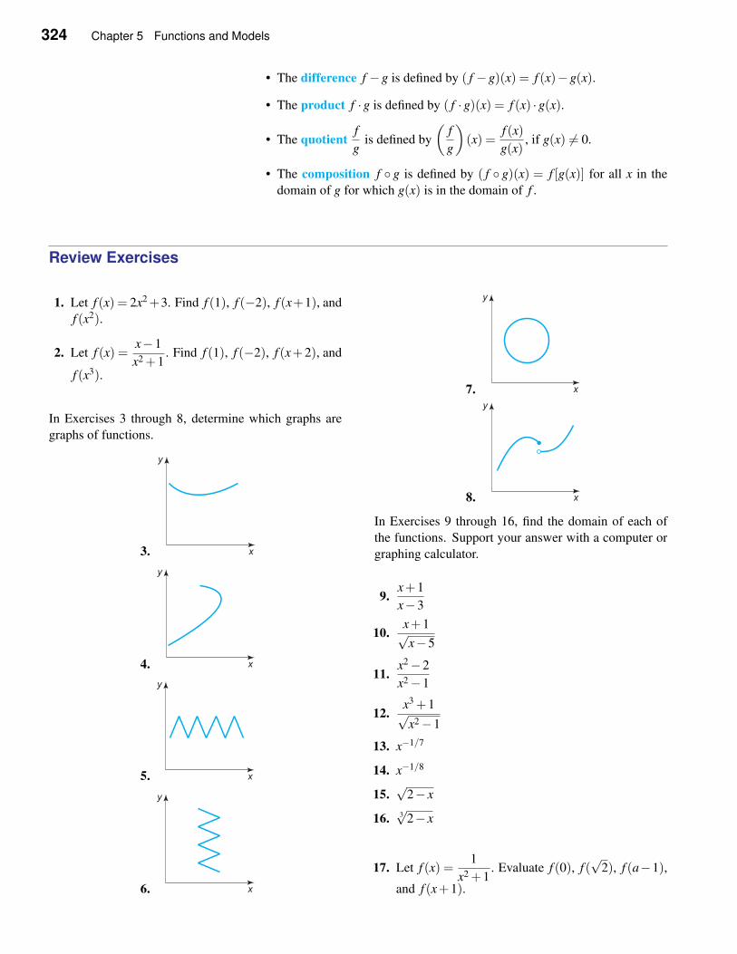
324 Chapter 5 Functions and Models
• The difference f −g is defined by ( f −g)(x) = f (x)−g(x).
• The product f ·g is defined by ( f ·g)(x) = f (x) ·g(x).
• The quotientf
gis defined by
(f
g
)
(x) =f (x)
g(x), if g(x) 6= 0.
• The composition f ◦ g is defined by ( f ◦ g)(x) = f [g(x)] for all x in the
domain of g for which g(x) is in the domain of f .
Review Exercises
1. Let f (x) = 2x2+3. Find f (1), f (−2), f (x+1), and
f (x2).
2. Let f (x) =x−1
x2 +1. Find f (1), f (−2), f (x+2), and
f (x3).
In Exercises 3 through 8, determine which graphs are
graphs of functions.
3.
4.
5.
6.
7.
8.
In Exercises 9 through 16, find the domain of each of
the functions. Support your answer with a computer or
graphing calculator.
9.x+1
x−3
10.x+1√x−5
11.x2−2
x2−1
12.x3 +1√x2−1
13. x−1/7
14. x−1/8
15.√
2− x
16. 3√
2− x
17. Let f (x) =1
x2 +1. Evaluate f (0), f (
√2), f (a−1),
and f (x+1).
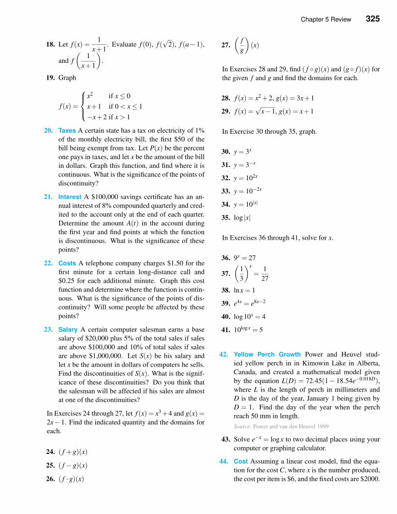
Chapter 5 Review 325
18. Let f (x) =1
x+1. Evaluate f (0), f (
√2), f (a− 1),
and f
(1
x+1
)
.
19. Graph
f (x) =
x2 if x≤ 0
x+1 if 0 < x≤ 1
−x+2 if x > 1
20. Taxes A certain state has a tax on electricity of 1%
of the monthly electricity bill, the first $50 of the
bill being exempt from tax. Let P(x) be the percent
one pays in taxes, and let x be the amount of the bill
in dollars. Graph this function, and find where it is
continuous. What is the significance of the points of
discontinuity?
21. Interest A $100,000 savings certificate has an an-
nual interest of 8% compounded quarterly and cred-
ited to the account only at the end of each quarter.
Determine the amount A(t) in the account during
the first year and find points at which the function
is discontinuous. What is the significance of these
points?
22. Costs A telephone company charges $1.50 for the
first minute for a certain long-distance call and
$0.25 for each additional minute. Graph this cost
function and determine where the function is contin-
uous. What is the significance of the points of dis-
continuity? Will some people be affected by these
points?
23. Salary A certain computer salesman earns a base
salary of $20,000 plus 5% of the total sales if sales
are above $100,000 and 10% of total sales if sales
are above $1,000,000. Let S(x) be his salary and
let x be the amount in dollars of computers he sells.
Find the discontinuities of S(x). What is the signif-
icance of these discontinuities? Do you think that
the salesman will be affected if his sales are almost
at one of the discontinuities?
In Exercises 24 through 27, let f (x) = x3+4 and g(x) =2x−1. Find the indicated quantity and the domains for
each.
24. ( f +g)(x)
25. ( f −g)(x)
26. ( f ·g)(x)
27.
(f
g
)
(x)
In Exercises 28 and 29, find ( f ◦g)(x) and (g◦ f )(x) for
the given f and g and find the domains for each.
28. f (x) = x2 +2, g(x) = 3x+1
29. f (x) =√
x−1, g(x) = x+1
In Exercise 30 through 35, graph.
30. y = 3x
31. y = 3−x
32. y = 102x
33. y = 10−2x
34. y = 10|x|
35. log |x|
In Exercises 36 through 41, solve for x.
36. 9x = 27
37.
(1
3
)x
=1
27
38. lnx = 1
39. e4x = e8x−2
40. log10x = 4
41. 10logx = 5
42. Yellow Perch Growth Power and Heuvel stud-
ied yellow perch in in Kimowin Lake in Alberta,
Canada, and created a mathematical model given
by the equation L(D) = 72.45(1− 18.54e−0.018D),where L is the length of perch in millimeters and
D is the day of the year, January 1 being given by
D = 1. Find the day of the year when the perch
reach 50 mm in length.
Source: Power and van den Heuvel 1999
43. Solve e−x = logx to two decimal places using your
computer or graphing calculator.
44. Cost Assuming a linear cost model, find the equa-
tion for the cost C, where x is the number produced,
the cost per item is $6, and the fixed costs are $2000.
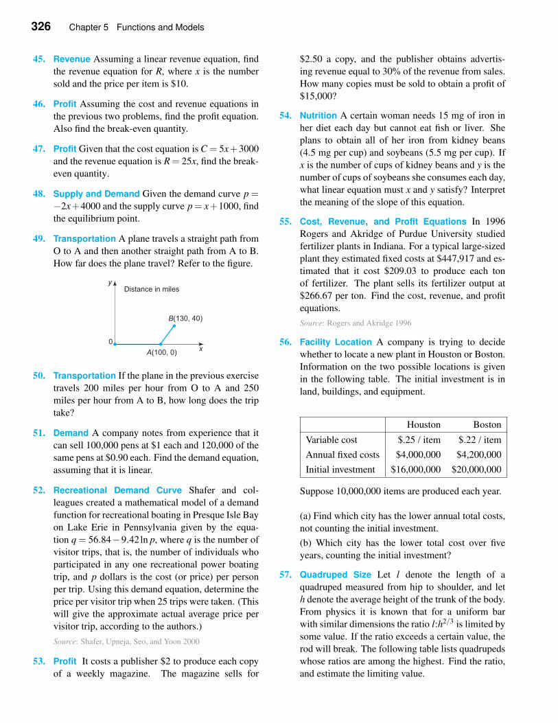
326 Chapter 5 Functions and Models
45. Revenue Assuming a linear revenue equation, find
the revenue equation for R, where x is the number
sold and the price per item is $10.
46. Profit Assuming the cost and revenue equations in
the previous two problems, find the profit equation.
Also find the break-even quantity.
47. Profit Given that the cost equation is C = 5x+3000
and the revenue equation is R = 25x, find the break-
even quantity.
48. Supply and Demand Given the demand curve p =−2x+4000 and the supply curve p = x+1000, find
the equilibrium point.
49. Transportation A plane travels a straight path from
O to A and then another straight path from A to B.
How far does the plane travel? Refer to the figure.
50. Transportation If the plane in the previous exercise
travels 200 miles per hour from O to A and 250
miles per hour from A to B, how long does the trip
take?
51. Demand A company notes from experience that it
can sell 100,000 pens at $1 each and 120,000 of the
same pens at $0.90 each. Find the demand equation,
assuming that it is linear.
52. Recreational Demand Curve Shafer and col-
leagues created a mathematical model of a demand
function for recreational boating in Presque Isle Bay
on Lake Erie in Pennsylvania given by the equa-
tion q = 56.84−9.42ln p, where q is the number of
visitor trips, that is, the number of individuals who
participated in any one recreational power boating
trip, and p dollars is the cost (or price) per person
per trip. Using this demand equation, determine the
price per visitor trip when 25 trips were taken. (This
will give the approximate actual average price per
visitor trip, according to the authors.)
Source: Shafer, Upneja, Seo, and Yoon 2000
53. Profit It costs a publisher $2 to produce each copy
of a weekly magazine. The magazine sells for
$2.50 a copy, and the publisher obtains advertis-
ing revenue equal to 30% of the revenue from sales.
How many copies must be sold to obtain a profit of
$15,000?
54. Nutrition A certain woman needs 15 mg of iron in
her diet each day but cannot eat fish or liver. She
plans to obtain all of her iron from kidney beans
(4.5 mg per cup) and soybeans (5.5 mg per cup). If
x is the number of cups of kidney beans and y is the
number of cups of soybeans she consumes each day,
what linear equation must x and y satisfy? Interpret
the meaning of the slope of this equation.
55. Cost, Revenue, and Profit Equations In 1996
Rogers and Akridge of Purdue University studied
fertilizer plants in Indiana. For a typical large-sized
plant they estimated fixed costs at $447,917 and es-
timated that it cost $209.03 to produce each ton
of fertilizer. The plant sells its fertilizer output at
$266.67 per ton. Find the cost, revenue, and profit
equations.
Source: Rogers and Akridge 1996
56. Facility Location A company is trying to decide
whether to locate a new plant in Houston or Boston.
Information on the two possible locations is given
in the following table. The initial investment is in
land, buildings, and equipment.
Houston Boston
Variable cost $.25 / item $.22 / item
Annual fixed costs $4,000,000 $4,200,000
Initial investment $16,000,000 $20,000,000
Suppose 10,000,000 items are produced each year.
(a) Find which city has the lower annual total costs,
not counting the initial investment.
(b) Which city has the lower total cost over five
years, counting the initial investment?
57. Quadruped Size Let l denote the length of a
quadruped measured from hip to shoulder, and let
h denote the average height of the trunk of the body.
From physics it is known that for a uniform bar
with similar dimensions the ratio l:h2/3 is limited by
some value. If the ratio exceeds a certain value, the
rod will break. The following table lists quadrupeds
whose ratios are among the highest. Find the ratio,
and estimate the limiting value.
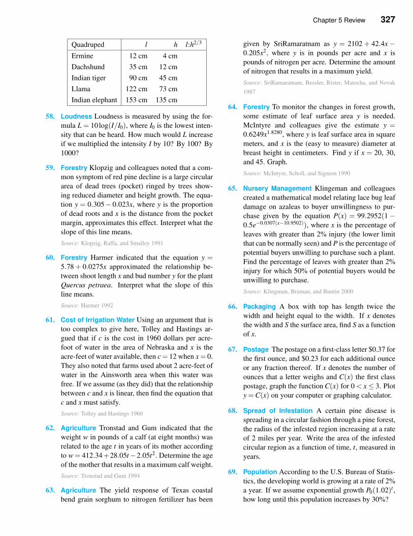
Chapter 5 Review 327
Quadruped l h l:h2/3
Ermine 12 cm 4 cm
Dachshund 35 cm 12 cm
Indian tiger 90 cm 45 cm
Llama 122 cm 73 cm
Indian elephant 153 cm 135 cm
58. Loudness Loudness is measured by using the for-
mula L = 10log(I/I0), where I0 is the lowest inten-
sity that can be heard. How much would L increase
if we multiplied the intensity I by 10? By 100? By
1000?
59. Forestry Klopzig and colleagues noted that a com-
mon symptom of red pine decline is a large circular
area of dead trees (pocket) ringed by trees show-
ing reduced diameter and height growth. The equa-
tion y = 0.305− 0.023x, where y is the proportion
of dead roots and x is the distance from the pocket
margin, approximates this effect. Interpret what the
slope of this line means.
Source: Klopzig, Raffa, and Smalley 1991
60. Forestry Harmer indicated that the equation y =5.78 + 0.0275x approximated the relationship be-
tween shoot length x and bud number y for the plant
Quercus petraea. Interpret what the slope of this
line means.
Source: Harmer 1992
61. Cost of Irrigation Water Using an argument that is
too complex to give here, Tolley and Hastings ar-
gued that if c is the cost in 1960 dollars per acre-
foot of water in the area of Nebraska and x is the
acre-feet of water available, then c= 12 when x= 0.
They also noted that farms used about 2 acre-feet of
water in the Ainsworth area when this water was
free. If we assume (as they did) that the relationship
between c and x is linear, then find the equation that
c and x must satisfy.
Source: Tolley and Hastings 1960
62. Agriculture Tronstad and Gum indicated that the
weight w in pounds of a calf (at eight months) was
related to the age t in years of its mother according
to w = 412.34+28.05t−2.05t2. Determine the age
of the mother that results in a maximum calf weight.
Source: Tronstad and Gum 1994
63. Agriculture The yield response of Texas coastal
bend grain sorghum to nitrogen fertilizer has been
given by SriRamaratnam as y = 2102 + 42.4x−0.205x2, where y is in pounds per acre and x is
pounds of nitrogen per acre. Determine the amount
of nitrogen that results in a maximum yield.
Source: SriRamaratnam, Bessler, Rister, Matocha, and Novak
1987
64. Forestry To monitor the changes in forest growth,
some estimate of leaf surface area y is needed.
McIntyre and colleagues give the estimate y =0.6249x1.8280, where y is leaf surface area in square
meters, and x is the (easy to measure) diameter at
breast height in centimeters. Find y if x = 20, 30,
and 45. Graph.
Source: McIntyre, Scholl, and Sigmon 1990
65. Nursery Management Klingeman and colleagues
created a mathematical model relating lace bug leaf
damage on azaleas to buyer unwillingness to pur-
chase given by the equation P(x) = 99.2952(1−0.5e−0.0307(x−10.9502)), where x is the percentage of
leaves with greater than 2% injury (the lower limit
that can be normally seen) and P is the percentage of
potential buyers unwilling to purchase such a plant.
Find the percentage of leaves with greater than 2%
injury for which 50% of potential buyers would be
unwilling to purchase.
Source: Klingman, Braman, and Buntin 2000
66. Packaging A box with top has length twice the
width and height equal to the width. If x denotes
the width and S the surface area, find S as a function
of x.
67. Postage The postage on a first-class letter $0.37 for
the first ounce, and $0.23 for each additional ounce
or any fraction thereof. If x denotes the number of
ounces that a letter weighs and C(x) the first class
postage, graph the function C(x) for 0 < x≤ 3. Plot
y =C(x) on your computer or graphing calculator.
68. Spread of Infestation A certain pine disease is
spreading in a circular fashion through a pine forest,
the radius of the infested region increasing at a rate
of 2 miles per year. Write the area of the infested
circular region as a function of time, t, measured in
years.
69. Population According to the U.S. Bureau of Statis-
tics, the developing world is growing at a rate of 2%
a year. If we assume exponential growth P0(1.02)t ,
how long until this population increases by 30%?
328 Chapter 5 Functions and Models
70. Population According to the U. S. Bureau of Statis-
tics, the population of India will double in 35 years.
If we assume exponential growth P0(1+ k)t , what
must be the growth constant k?
71. Population Growth According to the U.S. Bureau
of the Census, the population of Indonesia was 181
million in 1990 and growing at about 1.9% a year,
and the population of the United States was 249 mil-
lion in 1990 and growing at about 0.9% a year. Find
when the populations of these two countries will be
the same, assuming that the two growth rates con-
tinue at the given values.
72. Biology Gowen determined that the equation y =y0e−kr approximated the number of surviving to-
bacco viruses on tobacco plants where r is radiation
measured by r that the virus was exposed to and k
is a positive constant. What should be the radiation,
that is, the amount of r, that will kill 90% of the
virus. Your answer will be in terms of k.
Source: Kempthorne, Bancroft, Gowen, and Lush 1954
73. Biology Power and Heuvel developed a mathemat-
ical model given by the equation L(D) = 72.45(1−18.85e−0.018D), where L is the length in millimeters
of yellow perch hatched in the Spring in Kimowin
Lake in Alberta and D is the day of the year, D = 1
corresponding to January 1. The researchers were
interested in finding when the perch reached 80%
of their final length of 72.45 millimeters. Find the
time.
Source: Power and van den Heuvel 1999
74. Biology Wiedenmann and coworkers showed that
the proportion y of a certain host larvae parasitized
by Cotesian flavipes was approximated by y = 1−e−1.48x, where x is the parasite/host ratio. What ratio
results in 50% of the host being parasitized?
Source: Wiedenmann, Smith, and Darnell 1992
75. Soil Carbon Dynamics Knopps and Tilman stud-
ied the soil carbon dynamics of abandoned agri-
cultural fields and created a mathematical model
of soil carbon given by the equation C(t) =3.754
1+7.981e−0.0217t, where t is the number of years
after an agricultural field has been abandoned and
C(t) is the percentage of carbon in the soil. The
researchers asked how many years it would take to
bring the soil carbon percentage back to 95% of the
original. The original carbon in the soil was esti-
mated to be 3.754%. Answer this question.
Source: Knopps and Tilman 2000
✧ Diversity
Buoniorno and coworkers gave the index of tree size diversity
H =−[p1 ln p1 + p2 ln p2 + · · ·+ pn ln pn]
where pi is the proportion of trees in the ith size class.
(a) Is this index negative? Why or why not.
(b) Explain why this index does or does not equal
p1 ln1
p1+ p2 ln
1
p2+ · · ·+ pn ln
1
pn
(c) What is the value of this index if all the pi’s are equal?
(d) Suppose n = 2, p1 = p, and p2 = 1− p. What happens to H if p is close to
0? To 1? For what value of p is the diversity a minimum? Use your graphing
calculator to answer these questions. Explain why your answers makes sense in
view of the fact that H measures diversity.Source: Buongiorno, Dahir, Lu, and Lin 1994
Chapter 5 Review 329
✧ Evaporation of a Pollutant into the Atmosphere
Part of a pollutant in a body of water can, among other things, be absorbed by bottom sedi-
ment or be biodegraded through bacterial action. Other parts, however, may be released into the
atmosphere by evaporation. This pollutant evaporation can represent a serious problem, since, as
we will see, a very high percentage of certain pollutants pass into the atmosphere. Carried by the
wind and air currents, these pollutants can be carried for long distances and dramatically pollute
regions far from the source of the original contamination. The arctic regions, for example, are
suffering from this effect.
One model that is used is given by
(P
SPW−1
)
lnM
M0= ln
x
x0
where M is the amount of water and pollutant in the body of water with M0 the original amount,
x the pollutant concentration in the aqueous phases with x0 the original concentration, P is the
vapor pressure of the pure pollutant, PW is the vapor pressure of water, and S is the solubility of
the pollutant in water.
Notice thatM
M0× 100 is the percentage of water left, while
x
x0× 100 is the percentage of
pollutant left in the water.
Consider the example of mercury pollution. Mercury solubility at 25o C is 2.7× 10⁻⁹ mole
fraction. Mercury vapor pressure at the same temperature is 0.173Pa. Finally, water vapor pressure
at 25o C is 3170 Pa.
Assume that 0.01% of the body of water evaporates. (Note that this implies thatM
M0is
1
104.)
Find the concentration changex
x0. We are more interested in
(
1− x
x0
)
× 100, the percentage of
pollutant concentration in the vapor. Find this percentage. What can you say about this number?
Does this surprise you? What does this say about the significance of pollution by evaporation?
✧ Ground Penetration from an Oil Spill
Accidental oil spills on land (and water) are unfortunately becoming common. For an oil spill on
land, the strategy for cleanup operations will depend on the depth of the oil penetration in a given
time. The model presented here gives the time in seconds for the oil spill to penetrate a given
number of cm. We have
t =εµkρg
[L
1− ε− h
(1− ε)2ln
(
1+L(1− ε)
h
)]
where h is is the initial height (thickness) of the oil level in cm, L is the depth of the porous soil in
cm, ε is the porosity of the ground, k is the permeability of the ground in cm2, µ is the viscosity
of oil in kg/m3 in Pa, ρ the density of oil in kg/m3, and g = 9.81×10⁻⁴.
(a) Find the time if h = 6, L = .04, ε = 0.7, k = 10−6, µ = 0.02, ρ = 800.
(b) Find the time if we have a denser soil and h= 6, L = .04, ε = 0.1, k = 10−8, µ = 0.02, ρ = 800.
✧ Dynamics of Human Immunodeficiency Virus (HIV)
We consider here an early model of HIV dynamics that was developed about ten years ago. We
first give a brief description of the disease and its progress. A class of white blood cells known as T
cells are attacked by the HIV infection. T cells are important for the proper function of the immune
330 Chapter 5 Functions and Models
system. Following an infection, the immune system produces antibodies that can be detected in
the blood. Individuals with such antibodies are considered to be HIV positive.
Over a period that may last for years, the viral concentration remains relatively constant while
the T cell level slowly declines. At some point, however, the T cell decline may accelerate and
the virus concentration climb again. When the T cell count drops below 200 cells/mm3 (normal is
1000 cells/mm3), the patient is classified as having acquired immune deficiency syndrome (AIDS).
According to this model the progress of the viral concentration V depends of the sign and
magnitude of the roots of the following quadratic equation
x2 +(eT + eV )x+ eT (eV −NkU)
where U is the concentration of unaffected T cells, N is the number of viruses, k is a constant that
determines the rate at which cells are infected, eV is the rate of elimination or clearance of the
virus, and eT is the rate of elimination or clearance of infected T cells.
We assume conditions on all the constants that give rise to two different real roots of the
quadratic. Let a and b be the real roots of the quadratic. Then the model indicates that V will be in
the form V = Aeat +Bebt , where A and B are positive constants.
(a) Determine conditions on eV , N, k, and U that result in both roots being negative and thus the
concentration V of the virus steadily decreases. When you determine this condition, ask yourself
if your condition makes sense by varying the constants and determining the consequences. For
example, by making k smaller or eV larger, you expect the virus to decrease, or at least spread
more slowly. Is this true for your condition?
(b) Determine conditions on eV , N, k, and U that result in one positive root and one negative root.
What happens to V in this case? When you determine this condition, ask yourself if your condition
makes sense by varying the constants and determining the consequences. For example, by making
k largerer or eV smaller, you expect the concentration of the virus to eventually increase. Is this
true for your condition?
Comment: Notice from part (a) that AIDS is not an inevitable consequence of exposure to HIV.
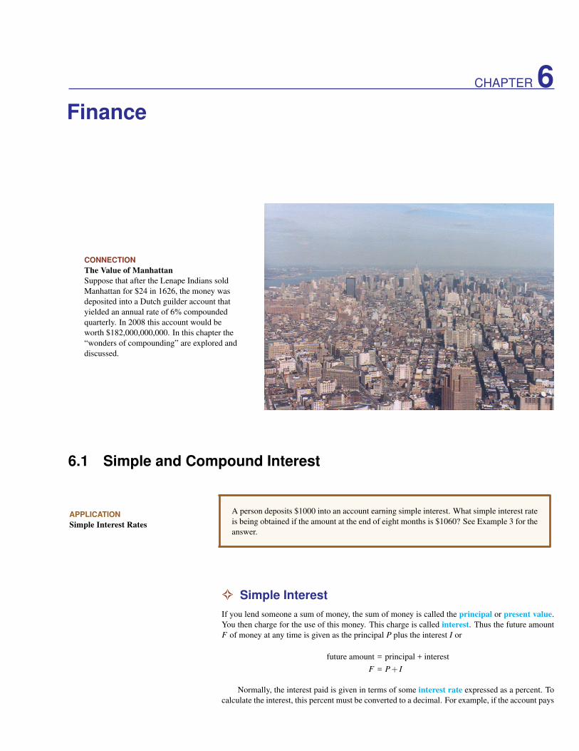
CHAPTER 6Finance
CONNECTION
The Value of Manhattan
Suppose that after the Lenape Indians sold
Manhattan for $24 in 1626, the money was
deposited into a Dutch guilder account that
yielded an annual rate of 6% compounded
quarterly. In 2008 this account would be
worth $182,000,000,000. In this chapter the
“wonders of compounding” are explored and
discussed.
6.1 Simple and Compound Interest
APPLICATION
Simple Interest Rates
A person deposits $1000 into an account earning simple interest. What simple interest rate
is being obtained if the amount at the end of eight months is $1060? See Example 3 for the
answer.
✧ Simple Interest
If you lend someone a sum of money, the sum of money is called the principal or present value.
You then charge for the use of this money. This charge is called interest. Thus the future amount
F of money at any time is given as the principal P plus the interest I or
future amount = principal + interest
F = P+ I
Normally, the interest paid is given in terms of some interest rate expressed as a percent. To
calculate the interest, this percent must be converted to a decimal. For example, if the account pays
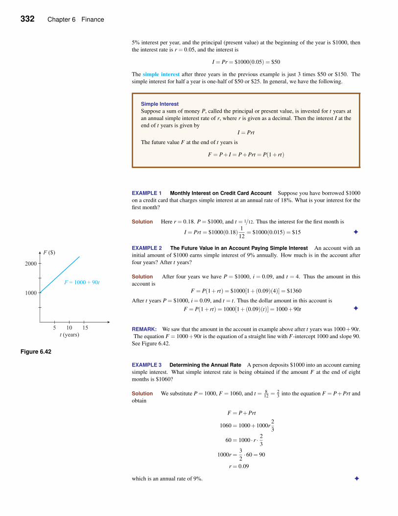
332 Chapter 6 Finance
5% interest per year, and the principal (present value) at the beginning of the year is $1000, then
the interest rate is r = 0.05, and the interest is
I = Pr = $1000(0.05) = $50
The simple interest after three years in the previous example is just 3 times $50 or $150. The
simple interest for half a year is one-half of $50 or $25. In general, we have the following.
Simple Interest
Suppose a sum of money P, called the principal or present value, is invested for t years at
an annual simple interest rate of r, where r is given as a decimal. Then the interest I at the
end of t years is given by
I = Prt
The future value F at the end of t years is
F = P+ I = P+Prt = P(1+ rt)
EXAMPLE 1 Monthly Interest on Credit Card Account Suppose you have borrowed $1000
on a credit card that charges simple interest at an annual rate of 18%. What is your interest for the
first month?
Solution Here r = 0.18. P = $1000, and t = 1/12. Thus the interest for the first month is
I = Prt = $1000(0.18)1
12= $1000(0.015) = $15 ✦
EXAMPLE 2 The Future Value in an Account Paying Simple Interest An account with an
initial amount of $1000 earns simple interest of 9% annually. How much is in the account after
four years? After t years?
Solution After four years we have P = $1000, i = 0.09, and t = 4. Thus the amount in this
account is
F = P(1+ rt) = $1000[1+(0.09)(4)] = $1360
After t years P = $1000, i = 0.09, and t = t. Thus the dollar amount in this account is
F = P(1+ rt) = 1000[1+(0.09)(t)] = 1000+90t ✦
REMARK: We saw that the amount in the account in example above after t years was 1000+90t.
The equation F = 1000+90t is the equation of a straight line with F-intercept 1000 and slope 90.
Figure 6.42
See Figure 6.42.
EXAMPLE 3 Determining the Annual Rate A person deposits $1000 into an account earning
simple interest. What simple interest rate is being obtained if the amount F at the end of eight
months is $1060?
Solution We substitute P = 1000, F = 1060, and t = 812 = 2
3 into the equation F = P+Prt and
obtain
F = P+Prt
1060 = 1000+1000r2
3
60 = 1000 · r · 23
1000r =3
2·60 = 90
r = 0.09
which is an annual rate of 9%. ✦
6.1 Simple and Compound Interest 333
✧ Present Value
Very often we find ourselves needing a certain amount of money at a specific time in the future.
We will now consider how to determine the present amount or present value of money needed to
deposit into an account earning simple interest in order to attain this future need. Suppose we need
the future amount F at the end of t years where money is deposited at a simple annual rate of r,
expressed as a decimal. Then to find the present amount needed to be deposited into this account,
we solve for P in the equation
F = P(1+ rt) → P =F
1+ rt
We then have the following.
Present Value
The present value needed to deposit into an account earning a simple annual rate of r,
expressed as a decimal, in order to have a future amount F after t years is
P =F
1+ rt
When asked how to amass $1
million the easy way, the banker
quipped “start with $950,000.”EXAMPLE 4 Present Value How much should be placed into an account paying simple
interest of 8% so that after six months the future value of the account will be $1,000,000?
Solution We have F = $1,000,000, r = 0.08, and t = 612 = 0.5. Thus
P =F
1+ rt=
$1,000,000
1+(0.08)(0.5)= $961,538.46
Thus you can have $1 million in this account in six months if you deposit $961,538.46 now. ✦
✧ A Mathematical Model of Compound Interest
We first consider how to calculate the most common type of interest, compound interest.
If the principal is invested for a period of time at an interest rate of i, where i is given as a
decimal, then the amount at the end of the first period is
principal + interest = P+Pi = P(1+ i)
The interest i is called the interest per period. If, for example, the annual interest for a bank
account is 6% and the time period is one month, then i = 0.0612 = 0.005 or 0.5% is the interest per
month.
If the interest and principal are left in the account for more than one period and interest is
calculated not only on the principal but also on the previous interest earned, we say that the interest
is being compounded.
If $1000 is deposited in a bank account earning interest at 6% a year and compounding
monthly, then, as we saw above, the interest is 0.5% per month, or 0.005 as a decimal. The
amount in the account at the end of any month is then always 1+0.005 = 1.005 times the amount
at the beginning of the month.
amount at end of month = [amount at beginning of month] × (1.005)
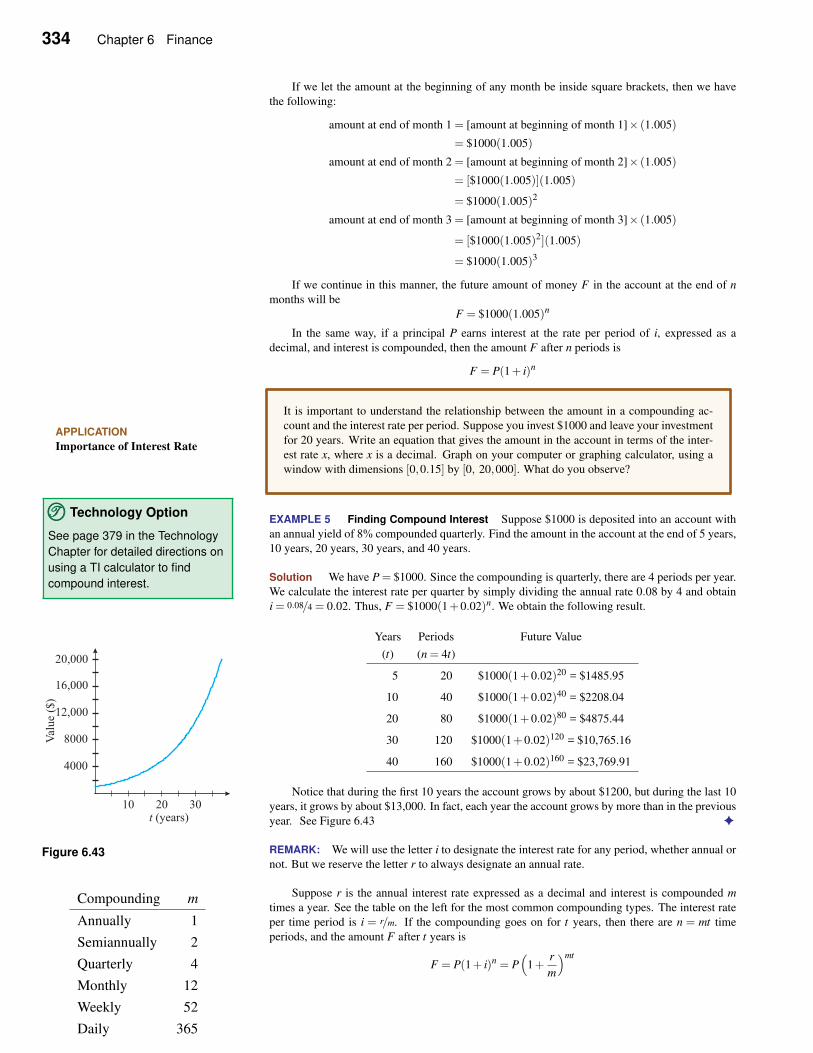
334 Chapter 6 Finance
If we let the amount at the beginning of any month be inside square brackets, then we have
the following:
amount at end of month 1 = [amount at beginning of month 1]× (1.005)
= $1000(1.005)
amount at end of month 2 = [amount at beginning of month 2]× (1.005)
= [$1000(1.005)](1.005)
= $1000(1.005)2
amount at end of month 3 = [amount at beginning of month 3]× (1.005)
= [$1000(1.005)2](1.005)
= $1000(1.005)3
If we continue in this manner, the future amount of money F in the account at the end of n
months will be
F = $1000(1.005)n
In the same way, if a principal P earns interest at the rate per period of i, expressed as a
decimal, and interest is compounded, then the amount F after n periods is
F = P(1+ i)n
APPLICATION
Importance of Interest Rate
It is important to understand the relationship between the amount in a compounding ac-
count and the interest rate per period. Suppose you invest $1000 and leave your investment
for 20 years. Write an equation that gives the amount in the account in terms of the inter-
est rate x, where x is a decimal. Graph on your computer or graphing calculator, using a
window with dimensions [0,0.15] by [0, 20,000]. What do you observe?
EXAMPLE 5 Finding Compound Interest Suppose $1000 is deposited into an account with
an annual yield of 8% compounded quarterly. Find the amount in the account at the end of 5 years,
10 years, 20 years, 30 years, and 40 years.
TTT©©© Technology Option
See page 379 in the Technology
Chapter for detailed directions on
using a TI calculator to find
compound interest.Solution We have P = $1000. Since the compounding is quarterly, there are 4 periods per year.
We calculate the interest rate per quarter by simply dividing the annual rate 0.08 by 4 and obtain
i = 0.08/4 = 0.02. Thus, F = $1000(1+0.02)n. We obtain the following result.
Years Periods Future Value
(t) (n = 4t)
5 20 $1000(1+0.02)20 = $1485.95
10 40 $1000(1+0.02)40 = $2208.04
20 80 $1000(1+0.02)80 = $4875.44
30 120 $1000(1+0.02)120 = $10,765.16
40 160 $1000(1+0.02)160 = $23,769.91
Notice that during the first 10 years the account grows by about $1200, but during the last 10
years, it grows by about $13,000. In fact, each year the account grows by more than in the previous
year. See Figure 6.43 ✦
Figure 6.43 REMARK: We will use the letter i to designate the interest rate for any period, whether annual or
not. But we reserve the letter r to always designate an annual rate.
Suppose r is the annual interest rate expressed as a decimal and interest is compounded m
times a year. See the table on the left for the most common compounding types. The interest rate
per time period is i = r/m. If the compounding goes on for t years, then there are n = mt time
periods, and the amount F after t years is
Compounding m
Annually 1
Semiannually 2
Quarterly 4
Monthly 12
Weekly 52
Daily 365
F = P(1+ i)n = P(
1+r
m
)mt
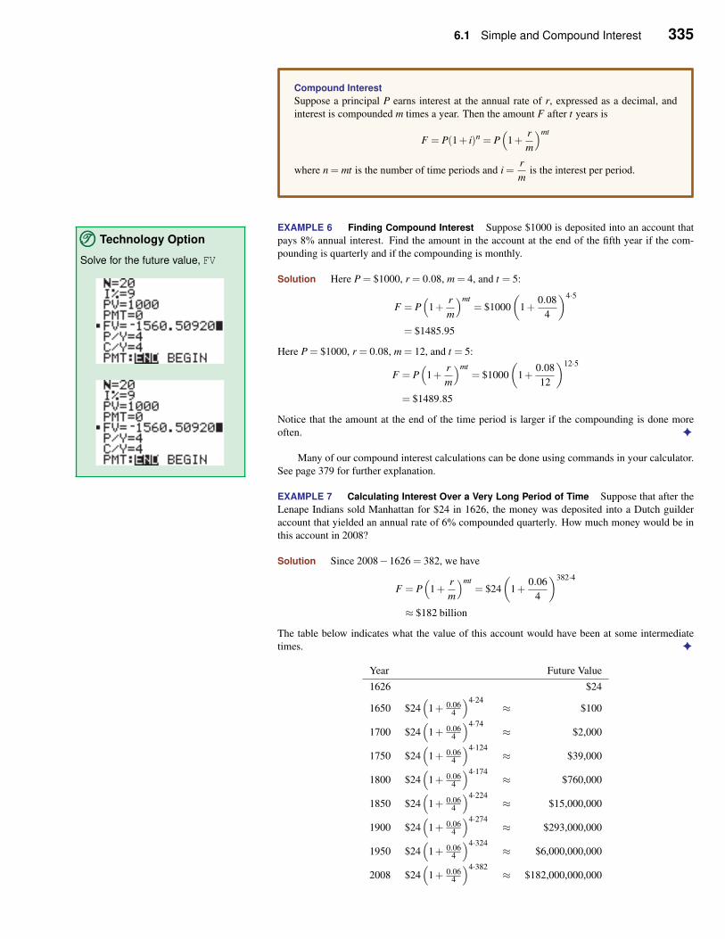
6.1 Simple and Compound Interest 335
Compound Interest
Suppose a principal P earns interest at the annual rate of r, expressed as a decimal, and
interest is compounded m times a year. Then the amount F after t years is
F = P(1+ i)n = P(
1+r
m
)mt
where n = mt is the number of time periods and i =r
mis the interest per period.
EXAMPLE 6 Finding Compound Interest Suppose $1000 is deposited into an account that
pays 8% annual interest. Find the amount in the account at the end of the fifth year if the com-
pounding is quarterly and if the compounding is monthly.
Solution Here P = $1000, r = 0.08, m = 4, and t = 5:
F = P(
1+r
m
)mt= $1000
(
1+0.08
4
)4·5
= $1485.95
Here P = $1000, r = 0.08, m = 12, and t = 5:
TTT©©© Technology Option
Solve for the future value, FV
F = P(
1+r
m
)mt= $1000
(
1+0.08
12
)12·5
= $1489.85
Notice that the amount at the end of the time period is larger if the compounding is done more
often. ✦
Many of our compound interest calculations can be done using commands in your calculator.
See page 379 for further explanation.
EXAMPLE 7 Calculating Interest Over a Very Long Period of Time Suppose that after the
Lenape Indians sold Manhattan for $24 in 1626, the money was deposited into a Dutch guilder
account that yielded an annual rate of 6% compounded quarterly. How much money would be in
this account in 2008?
Solution Since 2008−1626 = 382, we have
F = P(
1+r
m
)mt= $24
(
1+0.06
4
)382·4
≈ $182 billion
The table below indicates what the value of this account would have been at some intermediate
times. ✦
Year Future Value
1626 $24
1650 $24(
1+ 0.064
)4·24≈ $100
1700 $24(
1+ 0.064
)4·74≈ $2,000
1750 $24(
1+ 0.064
)4·124≈ $39,000
1800 $24(
1+ 0.064
)4·174≈ $760,000
1850 $24(
1+ 0.064
)4·224≈ $15,000,000
1900 $24(
1+ 0.064
)4·274≈ $293,000,000
1950 $24(
1+ 0.064
)4·324≈ $6,000,000,000
2008 $24(
1+ 0.064
)4·382≈ $182,000,000,000
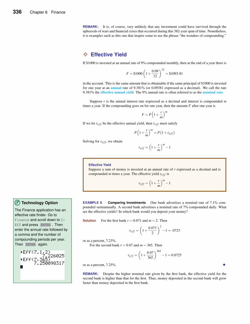
336 Chapter 6 Finance
REMARK: It is, of course, very unlikely that any investment could have survived through the
upheavals of wars and financial crises that occurred during this 382-year span of time. Nonetheless,
it is examples such as this one that inspire some to use the phrase “the wonders of compounding.”
✧ Effective Yield
If $1000 is invested at an annual rate of 9% compounded monthly, then at the end of a year there is
F = $1000
(
1+0.09
12
)12
= $1093.81
in the account. This is the same amount that is obtainable if the same principal of $1000 is invested
for one year at an annual rate of 9.381% (or 0.09381 expressed as a decimal). We call the rate
9.381% the effective annual yield. The 9% annual rate is often referred to as the nominal rate.
Suppose r is the annual interest rate expressed as a decimal and interest is compounded m
times a year. If the compounding goes on for one year, then the amount F after one year is
F = P(
1+r
m
)m
If we let re f f be the effective annual yield, then re f f must satisfy
P(
1+r
m
)m= P
(1+ re f f
)
Solving for re f f , we obtain
re f f =(
1+r
m
)m−1
Effective Yield
Suppose a sum of money is invested at an annual rate of r expressed as a decimal and is
compounded m times a year. The effective yield re f f is
re f f =(
1+r
m
)m−1
EXAMPLE 8 Comparing Investments One bank advertises a nominal rate of 7.1% com-
pounded semiannually. A second bank advertises a nominal rate of 7% compounded daily. What
are the effective yields? In which bank would you deposit your money?
Solution For the first bank r = 0.071 and m = 2. Then
re f f =
(
1+0.071
2
)2
−1 = .0723
or as a percent, 7.23%.
TTT©©© Technology Option
The Finance application has an
effective rate finder. Go to
Finance and scroll down to C:
Eff and press ENTER . Then
enter the annual rate followed by
a comma and the number of
compounding periods per year.
Then ENTER again. For the second bank r = 0.07 and m = 365. Then
re f f =
(
1+0.07
365
)365
−1 = 0.0725
or as a percent, 7.25%. ✦
REMARK: Despite the higher nominal rate given by the first bank, the effective yield for the
second bank is higher than that for the first. Thus, money deposited in the second bank will grow
faster than money deposited in the first bank.
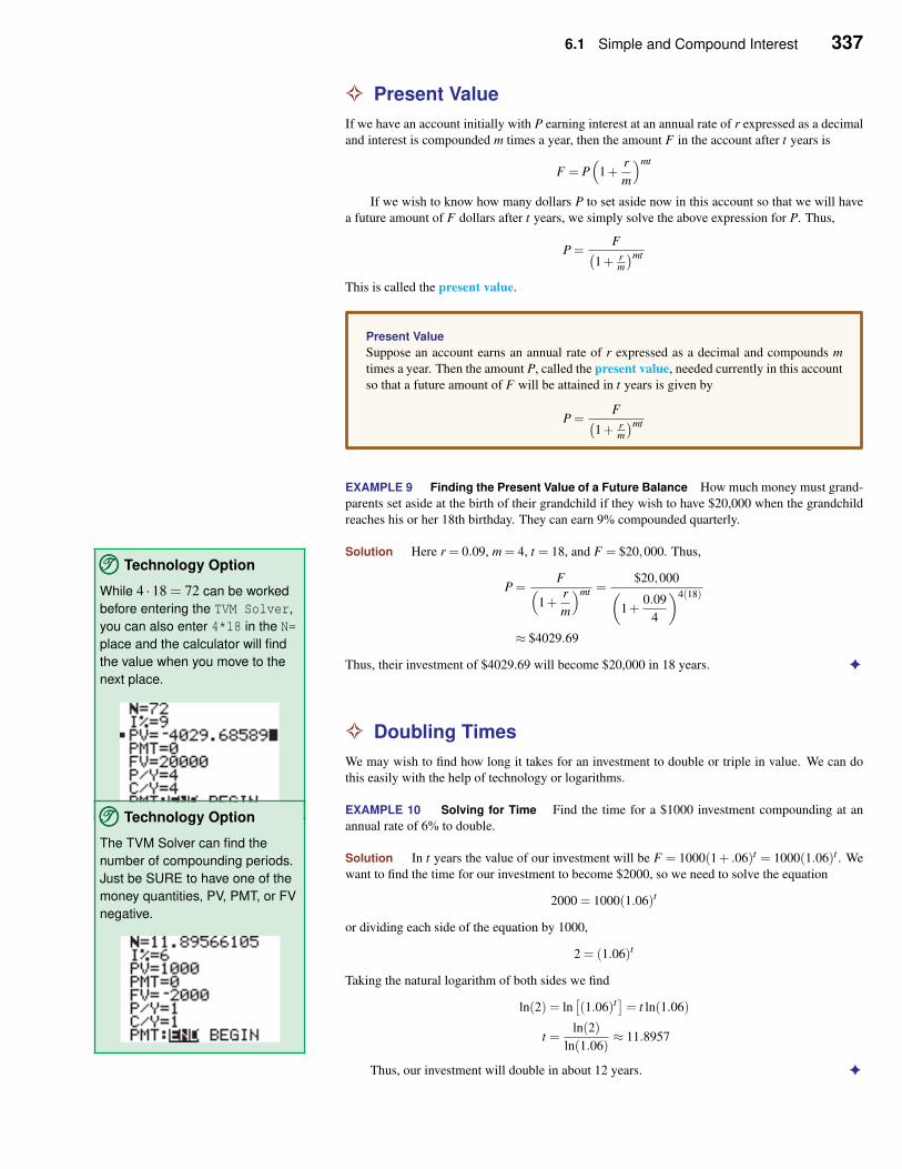
6.1 Simple and Compound Interest 337
✧ Present Value
If we have an account initially with P earning interest at an annual rate of r expressed as a decimal
and interest is compounded m times a year, then the amount F in the account after t years is
F = P(
1+r
m
)mt
If we wish to know how many dollars P to set aside now in this account so that we will have
a future amount of F dollars after t years, we simply solve the above expression for P. Thus,
P =F
(1+ r
m
)mt
This is called the present value.
Present Value
Suppose an account earns an annual rate of r expressed as a decimal and compounds m
times a year. Then the amount P, called the present value, needed currently in this account
so that a future amount of F will be attained in t years is given by
P =F
(1+ r
m
)mt
EXAMPLE 9 Finding the Present Value of a Future Balance How much money must grand-
parents set aside at the birth of their grandchild if they wish to have $20,000 when the grandchild
reaches his or her 18th birthday. They can earn 9% compounded quarterly.
Solution Here r = 0.09, m = 4, t = 18, and F = $20,000. Thus,TTT©©© Technology Option
While 4 ·18 = 72 can be worked
before entering the TVM Solver,
you can also enter 4*18 in the N=
place and the calculator will find
the value when you move to the
next place.
P =F
(
1+r
m
)mt =$20,000
(
1+0.09
4
)4(18)
≈ $4029.69
Thus, their investment of $4029.69 will become $20,000 in 18 years. ✦
✧ Doubling Times
We may wish to find how long it takes for an investment to double or triple in value. We can do
this easily with the help of technology or logarithms.
EXAMPLE 10 Solving for Time Find the time for a $1000 investment compounding at an
annual rate of 6% to double.
Solution In t years the value of our investment will be F = 1000(1+ .06)t = 1000(1.06)t . We
want to find the time for our investment to become $2000, so we need to solve the equation
2000 = 1000(1.06)t
or dividing each side of the equation by 1000,
TTT©©© Technology Option
The TVM Solver can find the
number of compounding periods.
Just be SURE to have one of the
money quantities, PV, PMT, or FV
negative.
2 = (1.06)t
Taking the natural logarithm of both sides we find
ln(2) = ln[(1.06)t
]= t ln(1.06)
t =ln(2)
ln(1.06)≈ 11.8957
Thus, our investment will double in about 12 years. ✦
338 Chapter 6 Finance
Self-Help Exercises 6.1
1. An account with $1000 earns interest at an annual rate of 8%.
Find the amount in this account after 10 years if the compound-
ing is
a. monthly b. daily.
2. Find the effective yield if the annual rate is 8% and the com-
pounding is weekly.
3. How much money should be deposited in a bank account earn-
ing an annual interest rate of 8% compounded quarterly so that
there will be $10,000 in the account at the end of 10 years?
6.1 Exercises
In Exercises 1 through 4, an amount of P dollars is borrowed for the
given length of time at an annual interest rate of r. Find the simple
interest that is owed.
1. P = $1000, r = 8.0%, 4 months
2. P = $2000, r = 6.0%, 3 months
3. P = $6000, r = 4.0%, 2 years
4. P = $5000, r = 7.0%, 3 years
In Exercises 5 through 8, an amount of P dollars is borrowed for the
given length of time at an annual simple interest rate of r. Find the
amount due at the end of the given length of time.
5. P = $2000, r = 4.0%, 7 months
6. P = $5000, r = 5.0%, 4 months
7. P = $1000, r = 6.0%, 2 years
8. P = $8000, r = 7.0%, 3 years
In Exercises 9 through 12, an amount of P dollars is borrowed for
the given length of time with the amount F due at the end of the
given length of time. Find the annual simple interest rate r.
9. P = $2000, F = $2100, 7 months
10. P = $5000, F = $5200, 4 months
11. P = $1000, F = $1070, 2 years
12. P = $8000, F = $9200, 3 years
In Exercises 13 through 16, find the present amount needed to at-
tain a future amount of F dollars in the given time using an annual
simple interest rate of r.
13. F = $2000, r = 4.0%, 3 months
14. F = $5000, r = 5.0%, 8 months
15. F = $6000, r = 6.0%, 2 years
16. F = $8000, r = 7.0%, 3 years
In Exercises 17 through 26, determine how much is in each account
on the basis of the indicated compounding after the specified years
have passed; P is the initial principal, and r is the annual rate given
as a percent.
17. P = $1000, r = 10%, compounded annually for 1 year.
18. P = $2000, r = 9%, compounded annually for 1 year.
19. After one year with, P = $1000 and r = 8%, compounded
a. annually b. quarterly c. monthly
d. weekly e. daily
20. After one year where P = $1000 and r = 10%, compounded
a. annually b. quarterly c. monthly
d. weekly e. daily
21. After 40 years where P = $1000 and r = 8%, compounded
a. annually b. quarterly c. monthly
d. weekly e. daily
22. After 40 years where P = $1000 and r = 10%, compounded
a. annually b. quarterly c. monthly
d. weekly e. daily
23. After 40 years where P = $1000, compounded annually, and r
is
a. 3% b. 5% c. 7% d. 9% e. 12% f. 15%
24. After 40 years where P = $1000, compounded annually, and r
is
a. 4% b. 6% c. 8% d. 10% e. 20% f. 25%
25. P = $1000 and r = 9%, compounded annually, after
a. 5 years b. 10 years c. 15 years d. 30 years
26. P = $1000 and r = 7%, compounded annually, after
a. 5 years b. 10 years c. 15 years d. 30 years
In Exercises 27 and 28, find the effective yield given the annual rate
r and the indicated compounding.
27. r = 8%, compounded
a. semiannually b. quarterly
c. monthly d. weekly
e. daily
6.1 Simple and Compound Interest 339
28. r = 10%, compounded
a. semiannually b. quarterly
c. monthly d. weekly
e. daily
In Exercises 29 through 32, find the present value of the given
amounts F with the indicated annual rate of return r, the number
of years t, and the indicated compounding.
29. F = $10,000, r = 9%, t = 20, compounded
a. annually b. monthly c. weekly
30. F = $10,000, r = 10%, t = 20, compounded
a. annually b. monthly c. weekly
31. F = $10,000, r = 9%, t = 40, compounded
a. annually b. monthly c. weekly
32. F = $10,000, r = 10%, t = 40, compounded
a. annually b. quarterly c. daily
33. Your rich uncle has just given you a high school graduation
present of $1 million. The present, however, is in the form of
a 40-year bond with an annual interest rate of 9% compounded
annually. The bond says that it will be worth $1 million in 40
years. What is this million-dollar gift worth at the present time?
34. Redo Exercise 33 if the annual interest rate is 6%.
35. Your rich aunt gives you a high school graduation present of $2
million. Her present is in the form of a 50-year bond with an
annual interest rate of 9%. The bond says that it will be worth
$2 million in 50 years. What is this gift worth at the present
time? Compare your answer to that in Exercise 33.
36. Redo Exercise 35 if the annual interest rate is 6%.
Applications
37. Future Value A principal of $5000 earns 8% per year simple
interest. How long will it take for the future value to become
$6000?
38. Future Value A principal of $2000 earns 6% per year simple
interest. How long will it take for the future value to become
$2300?
39. Doubling Time A principal earns 8% per year simple interest.
How long will it take for the future value to double?
40. Tripling Time A principal earns 6% per year simple interest.
How long will it take for the future value to triple?
41. Doubling Times Suppose you knew of an investment that
quadrupled in value in 18 years. What was the annual rate?
42. Doubling Times Suppose you knew of an investment that went
from $1000 to $8000 in 24 years. What was the annual rate?
In Exercises 43 and 44, Find the doubling time in years for the given
annual interest rates.
43. 2%
44. 3%
45. Find the time for an account earning interest at the annual rate
of 6% to grow from $1000 to $1500.
46. Find the time for an account earning interest at the annual rate
of 5% to grow from $1000 to $1600.
47. Real Estate Appreciation The United States paid about 4 cents
an acre for the Louisiana Purchase in 1803. Suppose the value
of this property grew at an annual rate of 5.5% compounded
annually. What would an acre be worth in 2010? Does this
seem realistic?
48. Real Estate Appreciation Redo previous exercise using a rate
of 6% instead of 5.5%. Compare your answer with the answer
to the previous exercise.
49. Appreciation Nancy’s $1000 investment grew at 8% a year for
about 9 years and then grew at 9% for an additional 8 years.
Find the value of her investment after 17 years.
50. Comparing Rates at Banks One bank advertises a nominal
rate of 6.5% compounded quarterly. A second bank advertises
a nominal rate of 6.6% compounded daily. What are the effec-
tive yields? In which bank would you deposit your money?
51. Comparing Rates at Banks One bank advertises a nominal
rate of 8.1% compounded semiannually. A second bank ad-
vertises a nominal rate of 8% compounded weekly. What are
the effective yields? In which bank would you deposit your
money?
52. Saving for Machinery How much money should a company
deposit in an account with a nominal rate of 8% compounded
quarterly in order to have $100,000 for a certain piece of ma-
chinery in five years?
53. Saving for Machinery Repeat the previous exercise with the
annual rate at 7% and compounding monthly.
Solutions to Self-Help Exercises 6.1
1. We have P = $1000, r = 0.08, t = 10, and m = 12. Thus, for monthly compounding
F = P(
1+r
m
)mt= 1000
(
1+0.08
12
)12·10
= 2219.64
TTT©©© Technology Option
The Self-Help Exercises can be
worked on the calculator
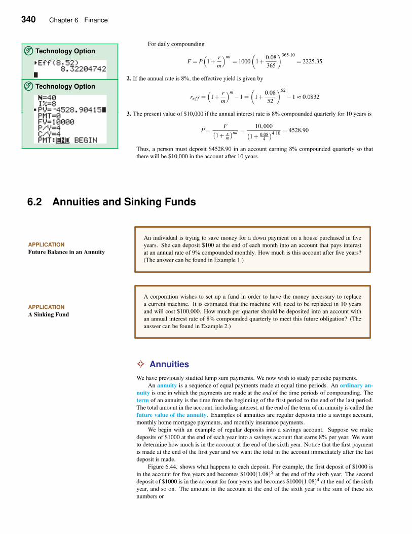
340 Chapter 6 Finance
For daily compounding
F = P(
1+r
m
)mt= 1000
(
1+0.08
365
)365·10
= 2225.35
2. If the annual rate is 8%, the effective yield is given by
TTT©©© Technology Option
re f f =(
1+r
m
)m−1 =
(
1+0.08
52
)52
−1≈ 0.0832
3. The present value of $10,000 if the annual interest rate is 8% compounded quarterly for 10 years is
TTT©©© Technology Option
P =F
(1+ r
m
)mt =10,000
(1+ 0.08
4
)4·10= 4528.90
Thus, a person must deposit $4528.90 in an account earning 8% compounded quarterly so that
there will be $10,000 in the account after 10 years.
6.2 Annuities and Sinking Funds
APPLICATION
Future Balance in an Annuity
An individual is trying to save money for a down payment on a house purchased in five
years. She can deposit $100 at the end of each month into an account that pays interest
at an annual rate of 9% compounded monthly. How much is this account after five years?
(The answer can be found in Example 1.)
APPLICATION
A Sinking Fund
A corporation wishes to set up a fund in order to have the money necessary to replace
a current machine. It is estimated that the machine will need to be replaced in 10 years
and will cost $100,000. How much per quarter should be deposited into an account with
an annual interest rate of 8% compounded quarterly to meet this future obligation? (The
answer can be found in Example 2.)
✧ Annuities
We have previously studied lump sum payments. We now wish to study periodic payments.
An annuity is a sequence of equal payments made at equal time periods. An ordinary an-
nuity is one in which the payments are made at the end of the time periods of compounding. The
term of an annuity is the time from the beginning of the first period to the end of the last period.
The total amount in the account, including interest, at the end of the term of an annuity is called the
future value of the annuity. Examples of annuities are regular deposits into a savings account,
monthly home mortgage payments, and monthly insurance payments.
We begin with an example of regular deposits into a savings account. Suppose we make
deposits of $1000 at the end of each year into a savings account that earns 8% per year. We want
to determine how much is in the account at the end of the sixth year. Notice that the first payment
is made at the end of the first year and we want the total in the account immediately after the last
deposit is made.
Figure 6.44. shows what happens to each deposit. For example, the first deposit of $1000 is
in the account for five years and becomes $1000(1.08)5 at the end of the sixth year. The second
deposit of $1000 is in the account for four years and becomes $1000(1.08)4 at the end of the sixth
year, and so on. The amount in the account at the end of the sixth year is the sum of these six
numbers or
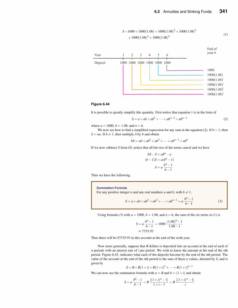
6.2 Annuities and Sinking Funds 341
S =1000+1000(1.08)+1000(1.08)2 +1000(1.08)3
+1000(1.08)4 +1000(1.08)5(1)
Figure 6.44
It is possible to greatly simplify this quantity. First notice that equation 1 is in the form of
S = a+ab+ab2 + · · ·+abn−2 +abn−1 (2)
where a = 1000, b = 1.08, and n = 6.
We now see how to find a simplified expression for any sum in the equation (2). If b = 1, then
S = na. If b 6= 1, then multiply S by b and obtain
bS = ab+ab2 +ab3 + · · ·+abn−1 +abn
If we now subtract S from bS, notice that all but two of the terms cancel and we have
bS−S = abn−a
(b−1)S = a(bn−1)
S = abn−1
b−1
Thus we have the following.
Summation Formula
For any positive integer n and any real numbers a and b, with b 6= 1,
S = a+ab+ab2 +ab3 + · · ·+abn−1 = abn−1
b−1(3)
Using formula (3) with a = 1000, b = 1.08, and n = 6, the sum of the six terms in (1) is
S = abn−1
b−1= 1000
(1.08)6−1
1.08−1
≈ 7335.93
Thus there will be $7335.93 in this account at the end of the sixth year.
Now more generally, suppose that R dollars is deposited into an account at the end of each of
n periods with an interest rate of i per period. We wish to know the amount at the end of the nth
period. Figure 6.45. indicates what each of the deposits become by the end of the nth period. The
value of the account at the end of the nth period is the sum of these n values, denoted by S, and is
given by
S = R+R(1+ i)+R(1+ i)2 + · · ·+R(1+ i)n−1
We can now use the summation formula with a = R and b = (1+ i) and obtain
S = abb−1
b−1= R
[(1+ i)n−1]
1+ i−1= R
[(1+ i)n−1]
i
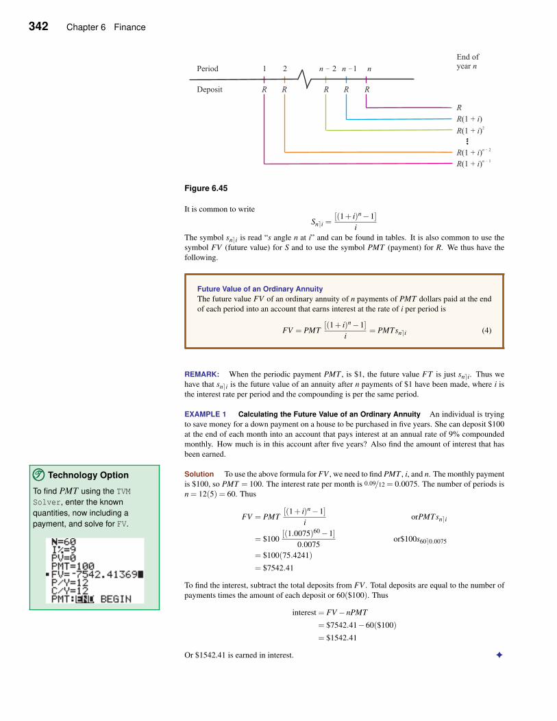
342 Chapter 6 Finance
Figure 6.45
It is common to write
Sn⌉i =[(1+ i)n−1]
i
The symbol sn⌉i is read “s angle n at i” and can be found in tables. It is also common to use the
symbol FV (future value) for S and to use the symbol PMT (payment) for R. We thus have the
following.
Future Value of an Ordinary Annuity
The future value FV of an ordinary annuity of n payments of PMT dollars paid at the end
of each period into an account that earns interest at the rate of i per period is
FV = PMT[(1+ i)n−1]
i= PMT sn⌉i (4)
REMARK: When the periodic payment PMT , is $1, the future value FT is just sn⌉i. Thus we
have that sn⌉i is the future value of an annuity after n payments of $1 have been made, where i is
the interest rate per period and the compounding is per the same period.
EXAMPLE 1 Calculating the Future Value of an Ordinary Annuity An individual is trying
to save money for a down payment on a house to be purchased in five years. She can deposit $100
at the end of each month into an account that pays interest at an annual rate of 9% compounded
monthly. How much is in this account after five years? Also find the amount of interest that has
been earned.
Solution To use the above formula for FV , we need to find PMT , i, and n. The monthly payment
is $100, so PMT = 100. The interest rate per month is 0.09/12 = 0.0075. The number of periods is
n = 12(5) = 60. Thus
TTT©©© Technology Option
To find PMT using the TVM
Solver, enter the known
quantities, now including a
payment, and solve for FV.FV = PMT
[(1+ i)n−1]
iorPMT sn⌉i
= $100[(1.0075)60−1]
0.0075or$100s60⌉0.0075
= $100(75.4241)
= $7542.41
To find the interest, subtract the total deposits from FV . Total deposits are equal to the number of
payments times the amount of each deposit or 60($100). Thus
interest = FV −nPMT
= $7542.41−60($100)
= $1542.41
Or $1542.41 is earned in interest. ✦
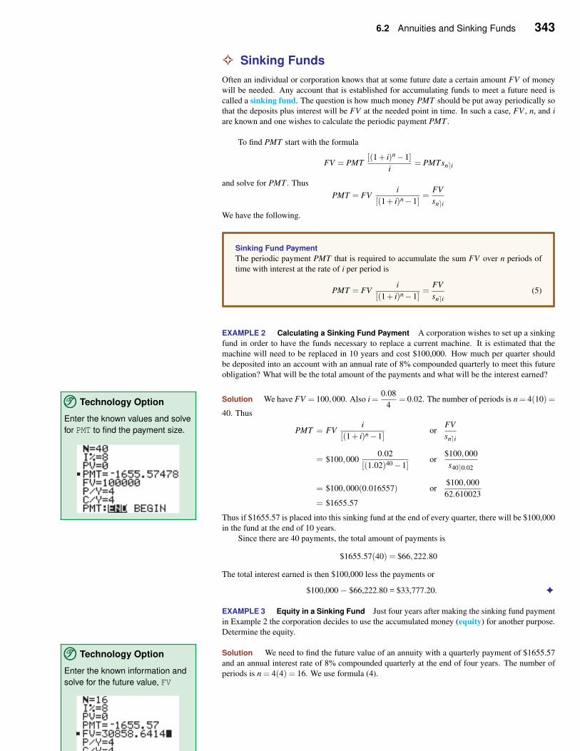
6.2 Annuities and Sinking Funds 343
✧ Sinking Funds
Often an individual or corporation knows that at some future date a certain amount FV of money
will be needed. Any account that is established for accumulating funds to meet a future need is
called a sinking fund. The question is how much money PMT should be put away periodically so
that the deposits plus interest will be FV at the needed point in time. In such a case, FV , n, and i
are known and one wishes to calculate the periodic payment PMT .
To find PMT start with the formula
FV = PMT[(1+ i)n−1]
i= PMT sn⌉i
and solve for PMT . Thus
PMT = FVi
[(1+ i)n−1]=
FV
sn⌉iWe have the following.
Sinking Fund Payment
The periodic payment PMT that is required to accumulate the sum FV over n periods of
time with interest at the rate of i per period is
PMT = FVi
[(1+ i)n−1]=
FV
sn⌉i(5)
EXAMPLE 2 Calculating a Sinking Fund Payment A corporation wishes to set up a sinking
fund in order to have the funds necessary to replace a current machine. It is estimated that the
machine will need to be replaced in 10 years and cost $100,000. How much per quarter should
be deposited into an account with an annual rate of 8% compounded quarterly to meet this future
obligation? What will be the total amount of the payments and what will be the interest earned?
Solution We have FV = 100,000. Also i =0.08
4= 0.02. The number of periods is n = 4(10) =
40. Thus
TTT©©© Technology Option
Enter the known values and solve
for PMT to find the payment size. PMT = FVi
[(1+ i)n−1]or
FV
sn⌉i
= $100,0000.02
[(1.02)40−1]or
$100,000
s40⌉0.02
= $100,000(0.016557) or$100,000
62.610023= $1655.57
Thus if $1655.57 is placed into this sinking fund at the end of every quarter, there will be $100,000
in the fund at the end of 10 years.
Since there are 40 payments, the total amount of payments is
$1655.57(40) = $66,222.80
The total interest earned is then $100,000 less the payments or
$100,000 − $66,222.80 = $33,777.20. ✦
EXAMPLE 3 Equity in a Sinking Fund Just four years after making the sinking fund payment
in Example 2 the corporation decides to use the accumulated money (equity) for another purpose.
Determine the equity.
Solution We need to find the future value of an annuity with a quarterly payment of $1655.57
and an annual interest rate of 8% compounded quarterly at the end of four years. The number of
periods is n = 4(4) = 16. We use formula (4).
TTT©©© Technology Option
Enter the known information and
solve for the future value, FV
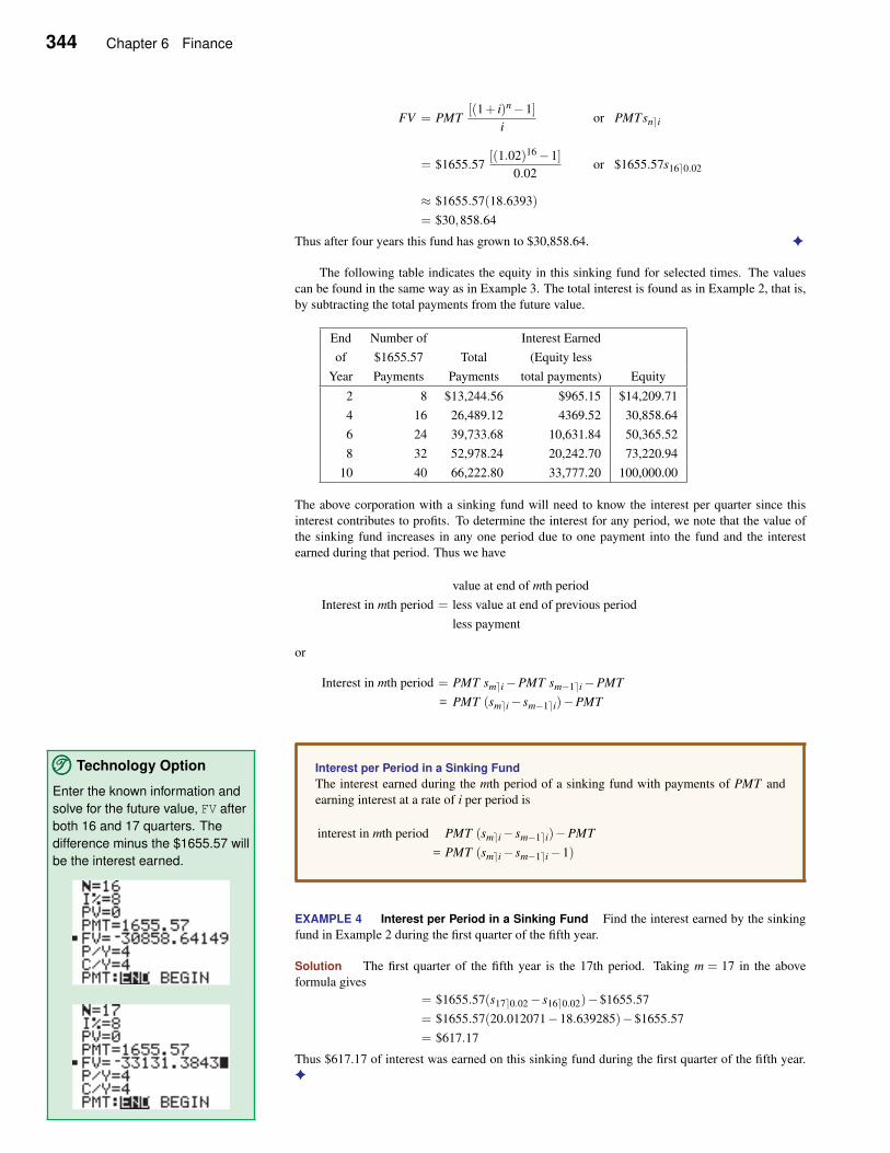
344 Chapter 6 Finance
FV = PMT[(1+ i)n−1]
ior PMT sn⌉i
= $1655.57[(1.02)16−1]
0.02or $1655.57s16⌉0.02
≈ $1655.57(18.6393)
= $30,858.64
Thus after four years this fund has grown to $30,858.64. ✦
The following table indicates the equity in this sinking fund for selected times. The values
can be found in the same way as in Example 3. The total interest is found as in Example 2, that is,
by subtracting the total payments from the future value.
End Number of Interest Earned
of $1655.57 Total (Equity less
Year Payments Payments total payments) Equity
2 8 $13,244.56 $965.15 $14,209.71
4 16 26,489.12 4369.52 30,858.64
6 24 39,733.68 10,631.84 50,365.52
8 32 52,978.24 20,242.70 73,220.94
10 40 66,222.80 33,777.20 100,000.00
The above corporation with a sinking fund will need to know the interest per quarter since this
interest contributes to profits. To determine the interest for any period, we note that the value of
the sinking fund increases in any one period due to one payment into the fund and the interest
earned during that period. Thus we have
value at end of mth period
Interest in mth period = less value at end of previous period
less payment
or
Interest in mth period = PMT sm⌉i−PMT sm−1⌉i−PMT
= PMT (sm⌉i− sm−1⌉i)−PMT
Interest per Period in a Sinking Fund
The interest earned during the mth period of a sinking fund with payments of PMT and
earning interest at a rate of i per period is
interest in mth period PMT (sm⌉i− sm−1⌉i)−PMT
= PMT (sm⌉i− sm−1⌉i−1)
EXAMPLE 4 Interest per Period in a Sinking Fund Find the interest earned by the sinking
fund in Example 2 during the first quarter of the fifth year.
TTT©©© Technology Option
Enter the known information and
solve for the future value, FV after
both 16 and 17 quarters. The
difference minus the $1655.57 will
be the interest earned.
Solution The first quarter of the fifth year is the 17th period. Taking m = 17 in the above
formula gives
= $1655.57(s17⌉0.02− s16⌉0.02)−$1655.57
= $1655.57(20.012071−18.639285)−$1655.57
= $617.17
Thus $617.17 of interest was earned on this sinking fund during the first quarter of the fifth year.
✦
6.2 Annuities and Sinking Funds 345
Self-Help Exercises 6.2
1. Every six months an individual places $1000 into an account
earning an annual rate of 10% compounded semiannually. Find
the amount in the account at the end of 15 years.
2. A person will need $20,000 to start a small business in five
years. How much should be deposited every three months into
an account paying an annual rate of 9% compounded quarterly
to meet this goal?
6.2 Exercises
In Exercises 1 through 6, find the future values of each of the ordi-
nary annuities at the given annual rate r compounded as indicated.
The payments are made to coincide with the periods of compound-
ing.
1. PMT = 1200, r = 0.08, compounded annually for 10 years
2. PMT = 600, r = 0.08, compounded semiannually for 10 years
3. PMT = 300, r = 0.08, compounded quarterly for 10 years
4. PMT = 100, r = 0.08, compounded monthly for 10 years
5. PMT = 100, r = 0.12, compounded monthly for 20 years
6. PMT = 100, r = 0.12, compounded weekly for 40 years
In Exercises 7 through 10, find the future value of each of the annu-
ities at the end of the given nth year where the payments are made
at the beginning of each year and r is the annual interest rate com-
pounded annually. Such an annuity is called an annuity due.
7. PMT = $1000, r = 0.08, 10 years
8. PMT = $1000, r = 0.10, 20 years
9. PMT = $1000, r = 0.15, 40 years
10. PMT = $500, r = 0.12, 30 years
In Exercises 11 through 16, find the periodic payment for each sink-
ing fund that is needed to accumulate the given sum under the given
conditions.
11. FV = $20,000, r = 0.09, compounded annually for 10 years
12. FV = $20,000, r = 0.09, compounded monthly for 20 years
13. FV = $10,000, r = 0.10, compounded quarterly for 10 years
14. FV = $1,000,000, r = 0.09, compounded weekly for 40 years
15. FV = $1,000,000, r = 0.15, compounded weekly for 40 years
16. FV = $1,000,000, r = 0.12, compounded monthly for 40 years
Applications
17. Retirement An individual earns an extra $2000 each year and
places this money at the end of each year into an Individual Re-
tirement Account (IRA) in which both the original earnings and
the interest in the account are not subject to taxation. If the ac-
count has an annual interest rate of 9% compounded annually,
how much is in the account at the end of 40 years?
18. Retirement Repeat the previous problem if the annual interest
rate is 12% per year.
19. Retirement Suppose the personal income tax is set at 33 13 %.
An individual earns an extra $2000 each year and pays income
taxes on these earnings and at the end of each year places the
remaining funds $2000( 23 ) into a regular savings account in
which the interest in the account is subject to the personal in-
come tax mentioned before. If the account earns an annual in-
terest rate of 9% compounded annually and the individual pays
income taxes owed on the interest out of these funds, how much
is in the account at the end of 40 years? Compare your answer
to Exercise 17.
20. Retirement Repeat the previous problem if the annual interest
rate is 12% per year. Compare your answer to Exercise 18.
21. Education Fund New parents wish to save for their newborn’s
education and wish to have $50,000 at the end of 18 years. How
much should they place at the end of each year into a savings
account that earns an annual rate of 9% compounded annually?
How much interest would they earn over the life of this ac-
count? Determine the equity in this fund after 10 years. How
much interest was earned during the 10th year?
22. Education Fund Repeat the previous problem if the annual in-
terest rate is 7%.
23. House Down Payment A couple will need $20,000 at the end
of five years for a down payment on a house. How much should
they place at the end of each month into a savings account earn-
ing an annual rate of 9% compounded monthly to meet this
goal? Determine the equity in this fund at the end of each year.
24. House Down Payment Repeat the previous problem if the an-
nual interest rate is 7%.
25. Equipment A corporation creates a sinking fund in order to
have $1 million to replace some machinery in 10 years. How
much should be placed into this account at the end of each quar-
ter if the annual interest rate is 10% compounded quarterly?
Determine the equity in this fund at the end of every 2 years.
How much interest was earned over the life of this fund? Deter-
mine the interest earned during the second quarter of the fifth
year.
26. Equipment Repeat the previous problem if the annual interest
rate is 6%.
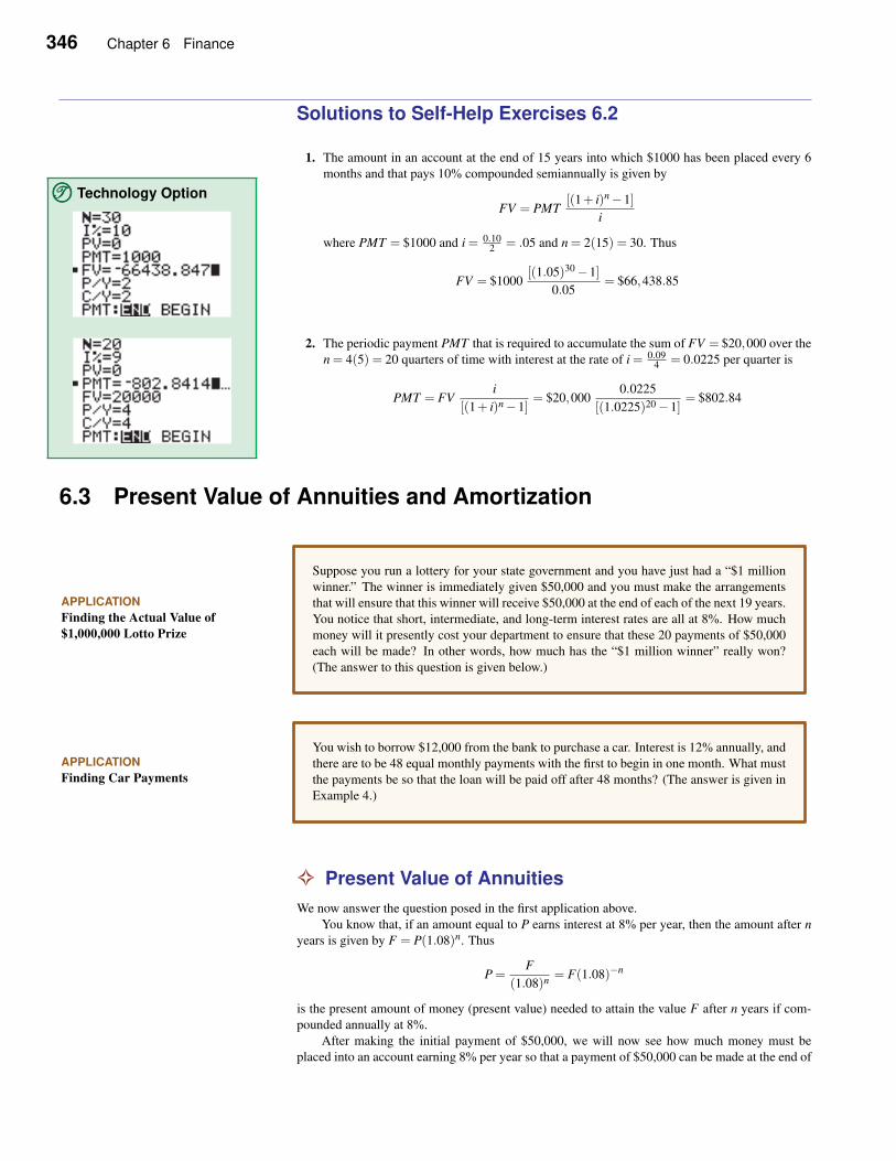
346 Chapter 6 Finance
Solutions to Self-Help Exercises 6.2
1. The amount in an account at the end of 15 years into which $1000 has been placed every 6
months and that pays 10% compounded semiannually is given by
FV = PMT[(1+ i)n−1]
i
where PMT = $1000 and i = 0.102 = .05 and n = 2(15) = 30. Thus
FV = $1000[(1.05)30−1]
0.05= $66,438.85
TTT©©© Technology Option
2. The periodic payment PMT that is required to accumulate the sum of FV = $20,000 over the
n = 4(5) = 20 quarters of time with interest at the rate of i = 0.094 = 0.0225 per quarter is
PMT = FVi
[(1+ i)n−1]= $20,000
0.0225
[(1.0225)20−1]= $802.84
6.3 Present Value of Annuities and Amortization
APPLICATION
Finding the Actual Value of
$1,000,000 Lotto Prize
Suppose you run a lottery for your state government and you have just had a “$1 million
winner.” The winner is immediately given $50,000 and you must make the arrangements
that will ensure that this winner will receive $50,000 at the end of each of the next 19 years.
You notice that short, intermediate, and long-term interest rates are all at 8%. How much
money will it presently cost your department to ensure that these 20 payments of $50,000
each will be made? In other words, how much has the “$1 million winner” really won?
(The answer to this question is given below.)
APPLICATION
Finding Car Payments
You wish to borrow $12,000 from the bank to purchase a car. Interest is 12% annually, and
there are to be 48 equal monthly payments with the first to begin in one month. What must
the payments be so that the loan will be paid off after 48 months? (The answer is given in
Example 4.)
✧ Present Value of Annuities
We now answer the question posed in the first application above.
You know that, if an amount equal to P earns interest at 8% per year, then the amount after n
years is given by F = P(1.08)n. Thus
P =F
(1.08)n= F(1.08)−n
is the present amount of money (present value) needed to attain the value F after n years if com-
pounded annually at 8%.
After making the initial payment of $50,000, we will now see how much money must be
placed into an account earning 8% per year so that a payment of $50,000 can be made at the end of
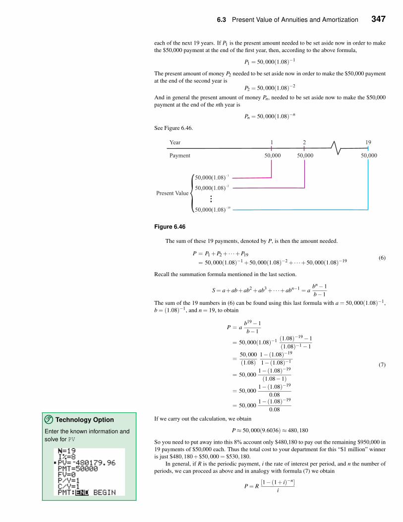
6.3 Present Value of Annuities and Amortization 347
each of the next 19 years. If P1 is the present amount needed to be set aside now in order to make
the $50,000 payment at the end of the first year, then, according to the above formula,
P1 = 50,000(1.08)−1
The present amount of money P2 needed to be set aside now in order to make the $50,000 payment
at the end of the second year is
P2 = 50,000(1.08)−2
And in general the present amount of money Pn, needed to be set aside now to make the $50,000
payment at the end of the nth year is
Pn = 50,000(1.08)−n
See Figure 6.46.
Figure 6.46
The sum of these 19 payments, denoted by P, is then the amount needed.
P = P1 +P2 + · · ·+P19
= 50,000(1.08)−1 +50,000(1.08)−2 + · · ·+50,000(1.08)−19(6)
Recall the summation formula mentioned in the last section.
S = a+ab+ab2 +ab3 + · · ·+abn−1 = abn−1
b−1
The sum of the 19 numbers in (6) can be found using this last formula with a = 50,000(1.08)−1,
b = (1.08)−1, and n = 19, to obtain
P = ab19−1
b−1
= 50,000(1.08)−1 (1.08)−19−1
(1.08)−1−1
=50,000
(1.08)
1− (1.08)−19
1− (1.08)−1
= 50,0001− (1.08)−19
(1.08−1)
= 50,0001− (1.08)−19
0.08
= 50,0001− (1.08)−19
0.08
(7)
If we carry out the calculation, we obtain
P≈ 50,000(9.6036)≈ 480,180
So you need to put away into this 8% account only $480,180 to pay out the remaining $950,000 in
19 payments of $50,000 each. Thus the total cost to your department for this “$1 million” winner
is just $480,180+$50,000 = $530,180.
TTT©©© Technology Option
Enter the known information and
solve for PV
In general, if R is the periodic payment, i the rate of interest per period, and n the number of
periods, we can proceed as above and in analogy with formula (7) we obtain
P = R[1− (1+ i)−n]
i
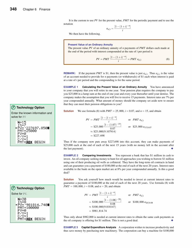
348 Chapter 6 Finance
It is the custom to use PV for the present value, PMT for the periodic payment and to use the
notation
an⌉i =[1− (1+ i)−n]
i
We then have the following.
Present Value of an Ordinary Annuity
The present value PV of an ordinary annuity of n payments of PMT dollars each made at
the end of the period with interest compounded at the rate of i per period is
PV = PMT[1− (1+ i)−n]
i= PMT an⌉i (8)
REMARK: If the payment PMT is $1, then the present value is just an⌉i. Thus an⌉i is the value
of an account needed to provide for n payments (or withdrawals) of $1 each when interest is paid
at a rate of i per period and the compounding is for the same period.
EXAMPLE 1 Calculating the Present Value of an Ordinary Annuity You have announced
to your company that you will retire in one year. Your pension plan requires the company to pay
you $25,000 in a lump sum at the end of one year and every year thereafter until your demise. The
company makes the assumption that you will live to receive 15 payments. Interest rates are 7% per
year compounded annually. What amount of money should the company set aside now to ensure
that they can meet their pension obligations to you?
Solution We use formula (8) with PMT = 25,000, i = 0.07, and n = 15, and obtainTTT©©© Technology Option
Enter the known information and
solve for PVPV = PMT
[1− (1+ i)−n]
ior PMT an⌉i
= $25,000[1− (1.07)−15]
0.07or $25,000 a15⌉0.07
≈ $25,000(9.107914)
= $227,698
Thus if the company now puts away $227,698 into this account, they can make payments of
$25,000 each at the end of each of the next 15 years (with no money left in the account after
the last payment). ✦
EXAMPLE 2 Comparing Investments You represent a bank that has $1 million in cash to
invest. An oil company seeking money to hunt for oil approaches you wishing to borrow $1 million
using one of their producing oil wells as collateral. They have the long-term oil contracts in hand
and can guarantee you a payment of $100,000 at the end of each of the next 20 years. Interest rates
available to the bank on the open market are at 8% per year compounded annually. Is this a good
deal?
Solution You ask yourself how much would be needed to invest at current interest rates to
guarantee a payment of $100,000 at the end of each of the next 20 years. Use formula (8) with
PMT = 100,000, i = 0.08, and n = 20, and obtainTTT©©© Technology Option
Solve for PV. PV = PMT[1− (1+ i)−n]
ior PMT an⌉i
= $100,000[1− (1.08)−20]
0.08or $100,000 a20⌉0.08
≈ $100,000(9.818147)
= $981,814.74
Thus only about $982,000 is needed at current interest rates to obtain the same cash payments as
the oil company is offering for $1 million. This is not a good deal. ✦
EXAMPLE 3 Capital Expenditure Analysis A corporation wishes to increase productivity and
thus save money by purchasing new machinery. The corporation can buy a machine for $100,000
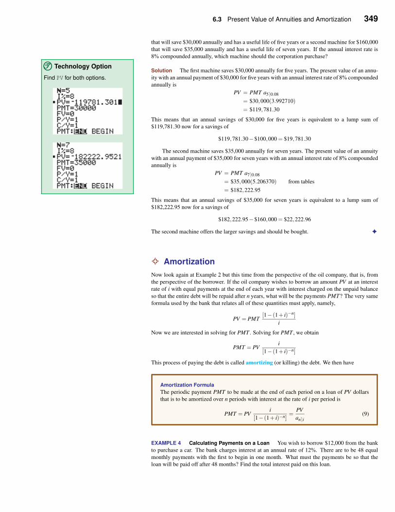
6.3 Present Value of Annuities and Amortization 349
that will save $30,000 annually and has a useful life of five years or a second machine for $160,000
that will save $35,000 annually and has a useful life of seven years. If the annual interest rate is
8% compounded annually, which machine should the corporation purchase?
Solution The first machine saves $30,000 annually for five years. The present value of an annu-
ity with an annual payment of $30,000 for five years with an annual interest rate of 8% compounded
annually is
PV = PMT a5⌉0.08
= $30,000(3.992710)
= $119,781.30
This means that an annual savings of $30,000 for five years is equivalent to a lump sum of
$119,781.30 now for a savings of
TTT©©© Technology Option
Find PV for both options.
$119,781.30−$100,000 = $19,781.30
The second machine saves $35,000 annually for seven years. The present value of an annuity
with an annual payment of $35,000 for seven years with an annual interest rate of 8% compounded
annually is
PV = PMT a7⌉0.08
= $35,000(5.206370) from tables
= $182,222.95
This means that an annual savings of $35,000 for seven years is equivalent to a lump sum of
$182,222.95 now for a savings of
$182,222.95−$160,000 = $22,222.96
The second machine offers the larger savings and should be bought. ✦
✧ Amortization
Now look again at Example 2 but this time from the perspective of the oil company, that is, from
the perspective of the borrower. If the oil company wishes to borrow an amount PV at an interest
rate of i with equal payments at the end of each year with interest charged on the unpaid balance
so that the entire debt will be repaid after n years, what will be the payments PMT ? The very same
formula used by the bank that relates all of these quantities must apply, namely,
PV = PMT[1− (1+ i)−n]
i
Now we are interested in solving for PMT . Solving for PMT , we obtain
PMT = PVi
[1− (1+ i)−n]
This process of paying the debt is called amortizing (or killing) the debt. We then have
Amortization Formula
The periodic payment PMT to be made at the end of each period on a loan of PV dollars
that is to be amortized over n periods with interest at the rate of i per period is
PMT = PVi
[1− (1+ i)−n]=
PV
an⌉i(9)
EXAMPLE 4 Calculating Payments on a Loan You wish to borrow $12,000 from the bank
to purchase a car. The bank charges interest at an annual rate of 12%. There are to be 48 equal
monthly payments with the first to begin in one month. What must the payments be so that the
loan will be paid off after 48 months? Find the total interest paid on this loan.
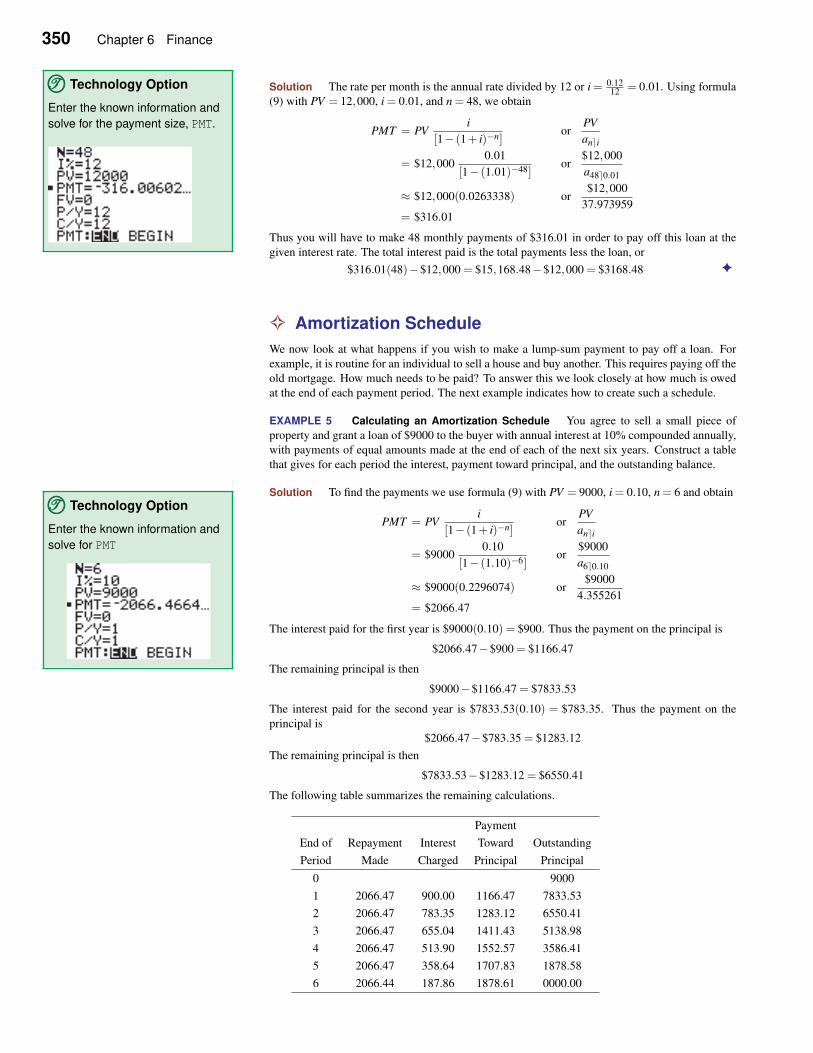
350 Chapter 6 Finance
Solution The rate per month is the annual rate divided by 12 or i = 0.1212 = 0.01. Using formula
(9) with PV = 12,000, i = 0.01, and n = 48, we obtain
TTT©©© Technology Option
Enter the known information and
solve for the payment size, PMT.PMT = PV
i
[1− (1+ i)−n]or
PV
an⌉i
= $12,0000.01
[1− (1.01)−48]or
$12,000
a48⌉0.01
≈ $12,000(0.0263338) or$12,000
37.973959= $316.01
Thus you will have to make 48 monthly payments of $316.01 in order to pay off this loan at the
given interest rate. The total interest paid is the total payments less the loan, or
$316.01(48)−$12,000 = $15,168.48−$12,000 = $3168.48 ✦
✧ Amortization Schedule
We now look at what happens if you wish to make a lump-sum payment to pay off a loan. For
example, it is routine for an individual to sell a house and buy another. This requires paying off the
old mortgage. How much needs to be paid? To answer this we look closely at how much is owed
at the end of each payment period. The next example indicates how to create such a schedule.
EXAMPLE 5 Calculating an Amortization Schedule You agree to sell a small piece of
property and grant a loan of $9000 to the buyer with annual interest at 10% compounded annually,
with payments of equal amounts made at the end of each of the next six years. Construct a table
that gives for each period the interest, payment toward principal, and the outstanding balance.
Solution To find the payments we use formula (9) with PV = 9000, i = 0.10, n = 6 and obtainTTT©©© Technology Option
Enter the known information and
solve for PMT
PMT = PVi
[1− (1+ i)−n]or
PV
an⌉i
= $90000.10
[1− (1.10)−6]or
$9000
a6⌉0.10
≈ $9000(0.2296074) or$9000
4.355261= $2066.47
The interest paid for the first year is $9000(0.10) = $900. Thus the payment on the principal is
$2066.47−$900 = $1166.47
The remaining principal is then
$9000−$1166.47 = $7833.53
The interest paid for the second year is $7833.53(0.10) = $783.35. Thus the payment on the
principal is
$2066.47−$783.35 = $1283.12
The remaining principal is then
$7833.53−$1283.12 = $6550.41
The following table summarizes the remaining calculations.
Payment
End of Repayment Interest Toward Outstanding
Period Made Charged Principal Principal
0 9000
1 2066.47 900.00 1166.47 7833.53
2 2066.47 783.35 1283.12 6550.41
3 2066.47 655.04 1411.43 5138.98
4 2066.47 513.90 1552.57 3586.41
5 2066.47 358.64 1707.83 1878.58
6 2066.44 187.86 1878.61 0000.00
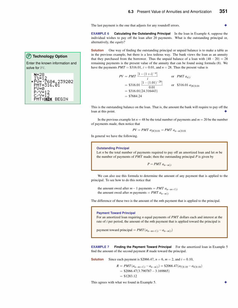
6.3 Present Value of Annuities and Amortization 351
The last payment is the one that adjusts for any roundoff errors. ✦
EXAMPLE 6 Calculating the Outstanding Principal In the loan in Example 4, suppose the
individual wishes to pay off the loan after 20 payments. What is the outstanding principal or,
alternatively, the equity?
Solution One way of finding the outstanding principal or unpaid balance is to make a table as
in the previous example, but there is a less tedious way. The bank views the loan as an annuity
that they purchased from the borrower. Thus the unpaid balance of a loan with (48− 20) = 28
remaining payments is the present value of the annuity that can be found using formula (8). We
have the payments PMT = $316.01, i = 0.01, and n = 28. Thus the present value is
PV = PMT[1− (1+ i)−n]
ior PMT an⌉i
= $316.01[1− (1.01)−28]
0.01or $316.01 a28⌉0.01
= $316.01(24.316443)
= $7684.24
TTT©©© Technology Option
Enter the known information and
solve for PV.
This is the outstanding balance on the loan. That is, the amount the bank will require to pay off the
loan at this point. ✦
In the previous example let n = 48 be the total number of payments and m = 20 be the number
of payments made, then notice that
PV = PMT a28⌉0.01 = PMT an−m⌉0.01
In general we have the following.
Outstanding Principal
Let n be the total number of payments required to pay off an amortized loan and let m be
the number of payments of PMT made; then the outstanding principal P is given by
P = PMT an−m⌉i
We can also use this formula to determine the amount of any payment that is applied to the
principal. To see how to do this notice that
the amount owed after m−1 payments = PMT an−m+1⌉ithe amount owed after m payments = PMT an−m⌉i
The difference of these two is the amount of the mth payment that is applied to the principal.
Payment Toward Principal
For an amortized loan requiring n equal payments of PMT dollars each and interest at the
rate of i per period, the amount of the mth payment that is applied toward the principal is
payment toward principal = PMT (an−m+1⌉i−an−m⌉i)
EXAMPLE 7 Finding the Payment Toward Principal For the amortized loan in Example 5
find the amount of the second payment R made toward the principal.
Solution Since each payment is $2066.47, n = 6, m = 2, and i = 0.10,
R = PMT (an−m+1⌉i−an−m⌉i) = $2066.47(a5⌉0.10−a4⌉0.10)
= $2066.47(3.790787−3.169865)
= $1283.12
This agrees with what we found in Example 5. ✦
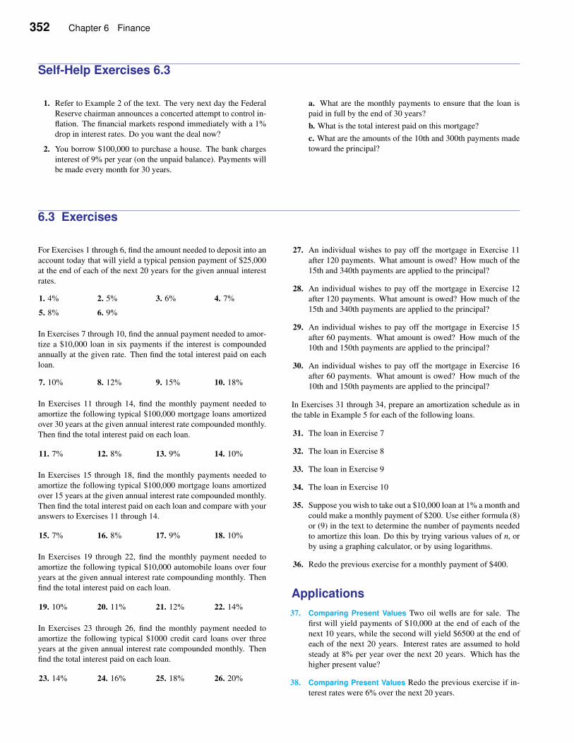
352 Chapter 6 Finance
Self-Help Exercises 6.3
1. Refer to Example 2 of the text. The very next day the Federal
Reserve chairman announces a concerted attempt to control in-
flation. The financial markets respond immediately with a 1%
drop in interest rates. Do you want the deal now?
2. You borrow $100,000 to purchase a house. The bank charges
interest of 9% per year (on the unpaid balance). Payments will
be made every month for 30 years.
a. What are the monthly payments to ensure that the loan is
paid in full by the end of 30 years?
b. What is the total interest paid on this mortgage?
c. What are the amounts of the 10th and 300th payments made
toward the principal?
6.3 Exercises
For Exercises 1 through 6, find the amount needed to deposit into an
account today that will yield a typical pension payment of $25,000
at the end of each of the next 20 years for the given annual interest
rates.
1. 4% 2. 5% 3. 6% 4. 7%
5. 8% 6. 9%
In Exercises 7 through 10, find the annual payment needed to amor-
tize a $10,000 loan in six payments if the interest is compounded
annually at the given rate. Then find the total interest paid on each
loan.
7. 10% 8. 12% 9. 15% 10. 18%
In Exercises 11 through 14, find the monthly payment needed to
amortize the following typical $100,000 mortgage loans amortized
over 30 years at the given annual interest rate compounded monthly.
Then find the total interest paid on each loan.
11. 7% 12. 8% 13. 9% 14. 10%
In Exercises 15 through 18, find the monthly payments needed to
amortize the following typical $100,000 mortgage loans amortized
over 15 years at the given annual interest rate compounded monthly.
Then find the total interest paid on each loan and compare with your
answers to Exercises 11 through 14.
15. 7% 16. 8% 17. 9% 18. 10%
In Exercises 19 through 22, find the monthly payment needed to
amortize the following typical $10,000 automobile loans over four
years at the given annual interest rate compounding monthly. Then
find the total interest paid on each loan.
19. 10% 20. 11% 21. 12% 22. 14%
In Exercises 23 through 26, find the monthly payment needed to
amortize the following typical $1000 credit card loans over three
years at the given annual interest rate compounded monthly. Then
find the total interest paid on each loan.
23. 14% 24. 16% 25. 18% 26. 20%
27. An individual wishes to pay off the mortgage in Exercise 11
after 120 payments. What amount is owed? How much of the
15th and 340th payments are applied to the principal?
28. An individual wishes to pay off the mortgage in Exercise 12
after 120 payments. What amount is owed? How much of the
15th and 340th payments are applied to the principal?
29. An individual wishes to pay off the mortgage in Exercise 15
after 60 payments. What amount is owed? How much of the
10th and 150th payments are applied to the principal?
30. An individual wishes to pay off the mortgage in Exercise 16
after 60 payments. What amount is owed? How much of the
10th and 150th payments are applied to the principal?
In Exercises 31 through 34, prepare an amortization schedule as in
the table in Example 5 for each of the following loans.
31. The loan in Exercise 7
32. The loan in Exercise 8
33. The loan in Exercise 9
34. The loan in Exercise 10
35. Suppose you wish to take out a $10,000 loan at 1% a month and
could make a monthly payment of $200. Use either formula (8)
or (9) in the text to determine the number of payments needed
to amortize this loan. Do this by trying various values of n, or
by using a graphing calculator, or by using logarithms.
36. Redo the previous exercise for a monthly payment of $400.
Applications
37. Comparing Present Values Two oil wells are for sale. The
first will yield payments of $10,000 at the end of each of the
next 10 years, while the second will yield $6500 at the end of
each of the next 20 years. Interest rates are assumed to hold
steady at 8% per year over the next 20 years. Which has the
higher present value?
38. Comparing Present Values Redo the previous exercise if in-
terest rates were 6% over the next 20 years.
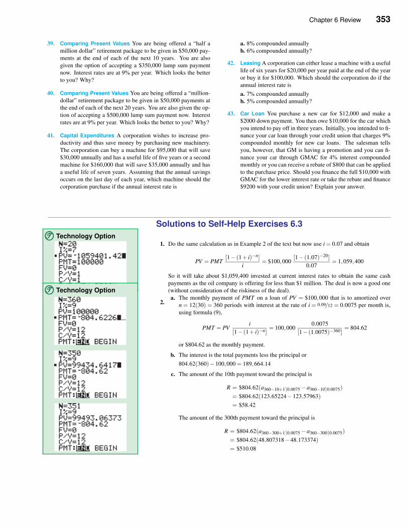
Chapter 6 Review 353
39. Comparing Present Values You are being offered a “half a
million dollar” retirement package to be given in $50,000 pay-
ments at the end of each of the next 10 years. You are also
given the option of accepting a $350,000 lump sum payment
now. Interest rates are at 9% per year. Which looks the better
to you? Why?
40. Comparing Present Values You are being offered a “million-
dollar” retirement package to be given in $50,000 payments at
the end of each of the next 20 years. You are also given the op-
tion of accepting a $500,000 lump sum payment now. Interest
rates are at 9% per year. Which looks the better to you? Why?
41. Capital Expenditures A corporation wishes to increase pro-
ductivity and thus save money by purchasing new machinery.
The corporation can buy a machine for $95,000 that will save
$30,000 annually and has a useful life of five years or a second
machine for $160,000 that will save $35,000 annually and has
a useful life of seven years. Assuming that the annual savings
occurs on the last day of each year, which machine should the
corporation purchase if the annual interest rate is
a. 8% compounded annually
b. 6% compounded annually?
42. Leasing A corporation can either lease a machine with a useful
life of six years for $20,000 per year paid at the end of the year
or buy it for $100,000. Which should the corporation do if the
annual interest rate is
a. 7% compounded annually
b. 5% compounded annually?
43. Car Loan You purchase a new car for $12,000 and make a
$2000 down payment. You then owe $10,000 for the car which
you intend to pay off in three years. Initially, you intended to fi-
nance your car loan through your credit union that charges 9%
compounded monthly for new car loans. The salesman tells
you, however, that GM is having a promotion and you can fi-
nance your car through GMAC for 4% interest compounded
monthly or you can receive a rebate of $800 that can be applied
to the purchase price. Should you finance the full $10,000 with
GMAC for the lower interest rate or take the rebate and finance
$9200 with your credit union? Explain your answer.
Solutions to Self-Help Exercises 6.3
1. Do the same calculation as in Example 2 of the text but now use i = 0.07 and obtain
TTT©©© Technology Option
PV = PMT[1− (1+ i)−n]
i= $100,000
[1− (1.07)−20]
0.07= 1,059,400
So it will take about $1,059,400 invested at current interest rates to obtain the same cash
payments as the oil company is offering for less than $1 million. The deal is now a good one
(without consideration of the riskiness of the deal).
2.a. The monthly payment of PMT on a loan of PV = $100,000 that is to amortized over
n = 12(30) = 360 periods with interest at the rate of i = 0.09/12 = 0.0075 per month is,
using formula (9),
PMT = PVi
[1− (1+ i)−n]= 100,000
0.0075
[1− (1.0075)−360]= 804.62
or $804.62 as the monthly payment.
TTT©©© Technology Option
b. The interest is the total payments less the principal or
804.62(360)−100,000 = 189,664.14
c. The amount of the 10th payment toward the principal is
R = $804.62(a360−10+1⌉0.0075−a360−10⌉0.0075)
= $804.62(123.65224−123.57963)
= $58.42
The amount of the 300th payment toward the principal is
R = $804.62(a360−300+1⌉0.0075−a360−300⌉0.0075)
= $804.62(48.807318−48.173374)
= $510.08
354 Chapter 6 Finance
Review
✧ Summary Outline
• Simple Interest. Suppose a sum of money P, called the principal or present value, is
invested for t years at an annual simple interest rate of r, where r is given as a decimal.
Then the interest I at the end of t years is given by
I = Prt
The future value F at the end of t years is
F = P+ I = P+Prt = P(l + rt)
• Present Value. The present value needed to deposit into an account earning a simple
annual rate of r, expressed as a decimal, in order to have a future amount F after t years is
P =F
1+ rt
• Compound Interest. Suppose a principal P earns interest at the annual rate of r, expressed
as a decimal, and interest is compounded m times a year. Then the amount F after t years
is
F = P(1+ i)n = P(
1+r
m
)mt
where n = mt is the number of time periods and i =r
mis the interest per period.
• Effective Yield. Suppose a sum of money is invested at an annual rate of r expressed as a
decimal and is compounded m times a year. The effective yield re f f is
re f f =(
1+r
m
)m−1
• Present Value. Suppose an account earns an annual rate of r expressed as a decimal and
is compounded m times a year. Then the amount P, called the present value, needed
presently in this account so that a future amount of F will be attained in t years is given by
P =F
(
1+r
m
)mt
• An annuity is a sequence of equal payments made at equal time periods.
• An ordinary annuity is one in which the payments are made at the end of the time periods
and the periods of compounding are the same time periods.
• The term of an annuity is the time from the beginning of the first period to the end of the
last period.
• The total amount in the account, including interest, at the end of the term of an annuity is
called the future value of the annuity.
• Summation Formula. For any positive integer n and any real numbers a and b with b 6= 1
a+ab+ab2 +ab3 + · · ·abn−1 = abn−1
b−1
• Future Value of an Ordinary Annuity. The future value FV of an ordinary annuity of n
payments of PMT dollars paid at the end of each period into a account that earns interest
at the rate of i per period is
FV = PMT[(1+ i)n−1]
i= PMT sn⌉i
• Sinking Fund Payment. The periodic payment PMT that is required to accumulate the
sum FV over n periods of time with interest at the rate of i per period is
PMT = FVi
[(1+ i)n−1]=
FV
sb⌉i
Chapter 6 Review 355
• Interest per Period in a Sinking Fund. The interest earned during the mth period of a
sinking fund with payments of PMT and earning interest at a rate of i per period is
Interest in mth period = PMT (sm⌉i− sm−1⌉i)−PMT
• Present Value of an Ordinary Annuity. The present value PV of an ordinary annuity of
n payments of PMT dollars each made at the end of the period with interest compounded
at the rate of i per period is
PV = PMT[1− (1+ i)−n]
i= PMT an⌉i
• Amortization Formula. The periodic payment PMT to be made at the end of each period
on a loan of PV dollars that is to be amortized over n periods with interest at the rate of i
per period is
PMT = PVi
[1− (1+ i)−n]=
PV
an⌉i
• Outstanding Principal. Let n be the total number of payments required to pay off an
amortized loan and let m be the number of payments of PMT made; then the outstanding
principal P is given by
P = PMT an−m⌉i
• Payment Toward Principal. For an amortized loan requiring n equal payments of PMT
dollars each and interest at the rate of i per period, the amount of the mth payment that is
applied toward the principal is
payment toward principal = PMT (an−m+1⌉i−an−m⌉i)
Review Exercises
In Exercises 1 through 2, find how much is in the following accounts
after the given t years where P is the initial principal, r is the annual
rate, and the compounding is as indicated.
1. t = 5, P = $1000, r = 8%, compounded
a. annually b. quarterly
c. monthly d. weekly
e. daily
2. t = 5, P = $1000, r = 10%, compounded
a. annually b. quarterly
c. monthly d. weekly
e. daily
In Exercises 3 through 4 find the effective yield given the annual rate
r and the indicated compounding.
3. r = 9%, compounded
a. semiannually b. quarterly
c. monthly d. weekly
e. daily
4. r = 11%, compounded
a. semiannually b. quarterly
c. monthly d. weekly
e. daily
In Exercises 5 through 6 find the present value of the given amounts
A with the indicated annual rate of return r, the number of years t,
and the indicated compounding.
5. A = $10,000, r = 8%, t = 10, compounded
a. annually b. monthly c. weekly
6. A = $10,000, r = 9%, t = 10, compounded
a. annually b. quarterly c. daily
7. You have just won a $1,000,000 lottery. Your entire prize will
be given to you in 20 years in a lump sum. If current inter-
est rates are 8% compounded annually, what is this $1,000,000
prize worth at the present?
8. How much money should you deposit now in an account earn-
ing 9% annually in order to have $10,000 in 5 years?
9. What annual rate is required for an account that is compounded
annually to double in 8 years?
10. Savings A self-employed individual places $3000 a year into
a Keogh account in which taxes are not paid on the interest. If
interest rates remain at 9%, how much will be in this account
after 30 years?
11. Sinking Fund A large corporation creates a sinking fund in or-
der to have a $2 million cash bonus for the president of the
company on his retirement in 10 years. How much should be
placed into this account at the end of each quarter if the interest
rate is 8% compounded quarterly? Over the life of this sink-
ing fund how much interest accumulates? How much interest
is earned in the third quarter of the fifth year?

356 Chapter 6 Finance
12. Lottery Prize The state lottery has just had a $2 million win-
ner and needs to pay the recipient $100,000 now and the same
amount at the end of each of the next 19 years. The state does
not wish to be involved in the administration of this disburse-
ment and wishes to give this obligation together with a lump
sum payment to an insurance company to handle the payments.
You are an investment advisor for an insurance company. Inter-
est rates are at 8%. What is the very least that you would accept
for this obligation?
13. Amortization You plan to borrow $100,000 to buy a house. In-
terest rates are at 9% a year compounded monthly. What will
be your monthly payments if the length of the mortgage is 25
years? 15 years? What will be the total interest paid in each
case? In each case how much of the 10th payment will go to-
ward the principal? The 120th?
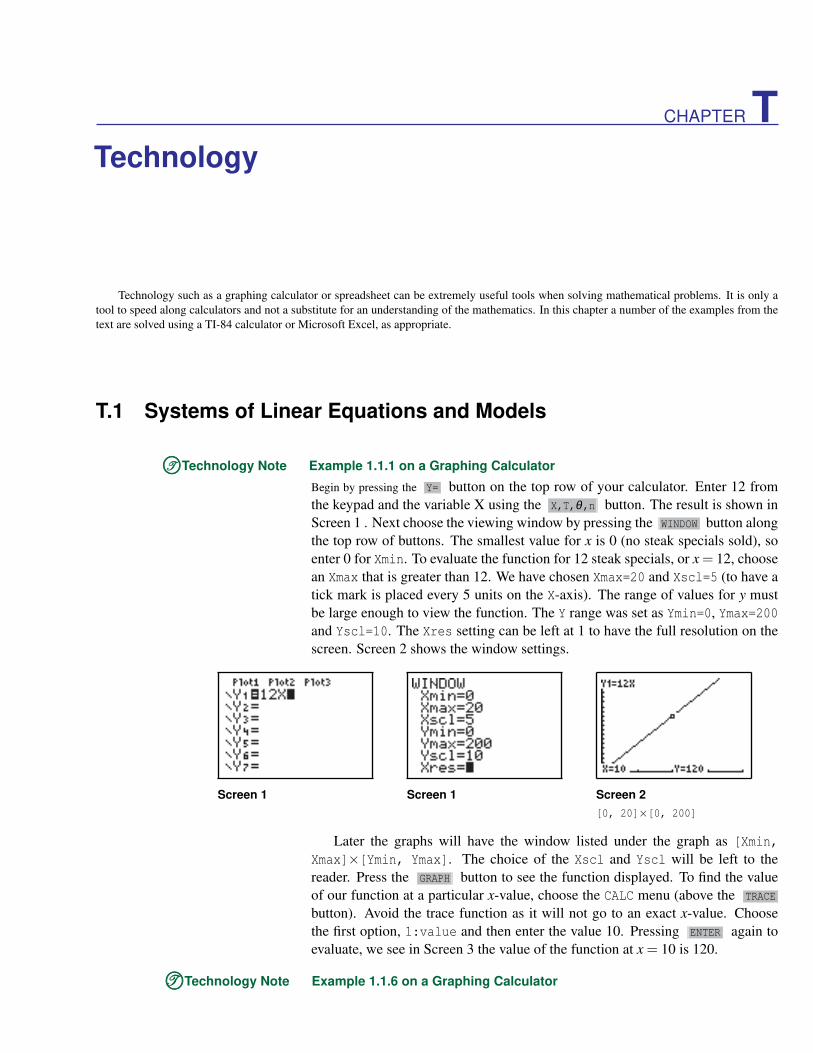
CHAPTER TTechnology
Technology such as a graphing calculator or spreadsheet can be extremely useful tools when solving mathematical problems. It is only a
tool to speed along calculators and not a substitute for an understanding of the mathematics. In this chapter a number of the examples from the
text are solved using a TI-84 calculator or Microsoft Excel, as appropriate.
T.1 Systems of Linear Equations and Models
TTT©©©Technology Note Example 1.1.1 on a Graphing Calculator
Begin by pressing the Y= button on the top row of your calculator. Enter 12 from
the keypad and the variable X using the X,T,θ,n button. The result is shown in
Screen 1 . Next choose the viewing window by pressing the WINDOW button along
the top row of buttons. The smallest value for x is 0 (no steak specials sold), so
enter 0 for Xmin. To evaluate the function for 12 steak specials, or x = 12, choose
an Xmax that is greater than 12. We have chosen Xmax=20 and Xscl=5 (to have a
tick mark is placed every 5 units on the X-axis). The range of values for y must
be large enough to view the function. The Y range was set as Ymin=0, Ymax=200
and Yscl=10. The Xres setting can be left at 1 to have the full resolution on the
screen. Screen 2 shows the window settings.
Screen 1 Screen 1 Screen 2
[0, 20]×[0, 200]
Later the graphs will have the window listed under the graph as [Xmin,
Xmax]×[Ymin, Ymax]. The choice of the Xscl and Yscl will be left to the
reader. Press the GRAPH button to see the function displayed. To find the value
of our function at a particular x-value, choose the CALC menu (above the TRACE
button). Avoid the trace function as it will not go to an exact x-value. Choose
the first option, 1:value and then enter the value 10. Pressing ENTER again to
evaluate, we see in Screen 3 the value of the function at x = 10 is 120.
TTT©©©Technology Note Example 1.1.6 on a Graphing Calculator
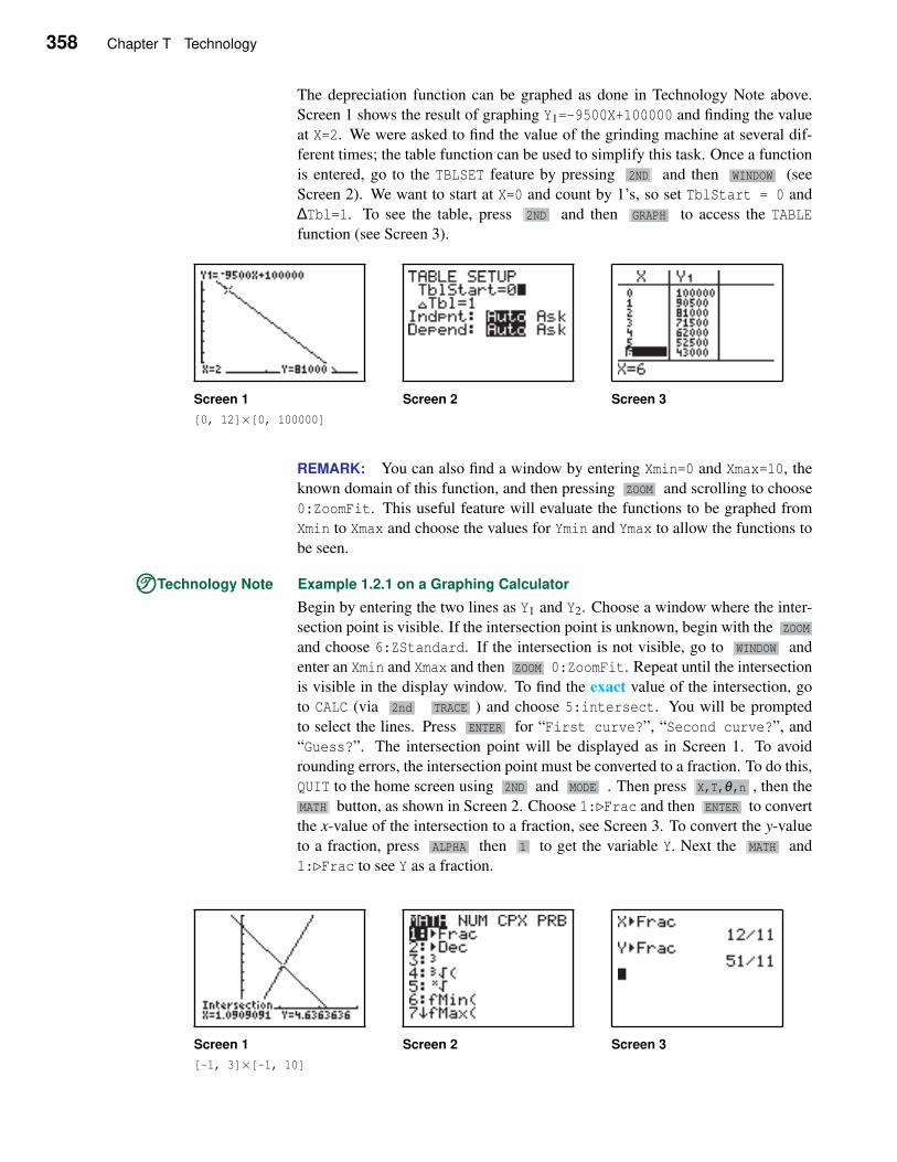
358 Chapter T Technology
The depreciation function can be graphed as done in Technology Note above.
Screen 1 shows the result of graphing Y1=-9500X+100000 and finding the value
at X=2. We were asked to find the value of the grinding machine at several dif-
ferent times; the table function can be used to simplify this task. Once a function
is entered, go to the TBLSET feature by pressing 2ND and then WINDOW (see
Screen 2). We want to start at X=0 and count by 1’s, so set TblStart = 0 and
∆Tbl=1. To see the table, press 2ND and then GRAPH to access the TABLE
function (see Screen 3).
Screen 1
[0, 12]×[0, 100000]
Screen 2 Screen 3
REMARK: You can also find a window by entering Xmin=0 and Xmax=10, the
known domain of this function, and then pressing ZOOM and scrolling to choose
0:ZoomFit. This useful feature will evaluate the functions to be graphed from
Xmin to Xmax and choose the values for Ymin and Ymax to allow the functions to
be seen.
TTT©©©Technology Note Example 1.2.1 on a Graphing Calculator
Begin by entering the two lines as Y1 and Y2. Choose a window where the inter-
section point is visible. If the intersection point is unknown, begin with the ZOOM
and choose 6:ZStandard. If the intersection is not visible, go to WINDOW and
enter an Xmin and Xmax and then ZOOM 0:ZoomFit. Repeat until the intersection
is visible in the display window. To find the exact value of the intersection, go
to CALC (via 2nd TRACE ) and choose 5:intersect. You will be prompted
to select the lines. Press ENTER for “First curve?”, “Second curve?”, and
“Guess?”. The intersection point will be displayed as in Screen 1. To avoid
rounding errors, the intersection point must be converted to a fraction. To do this,
QUIT to the home screen using 2ND and MODE . Then press X,T,θ,n , then the
MATH button, as shown in Screen 2. Choose 1:⊲Frac and then ENTER to convert
the x-value of the intersection to a fraction, see Screen 3. To convert the y-value
to a fraction, press ALPHA then 1 to get the variable Y. Next the MATH and
1:⊲Frac to see Y as a fraction.
Screen 1
[-1, 3]×[-1, 10]
Screen 2 Screen 3
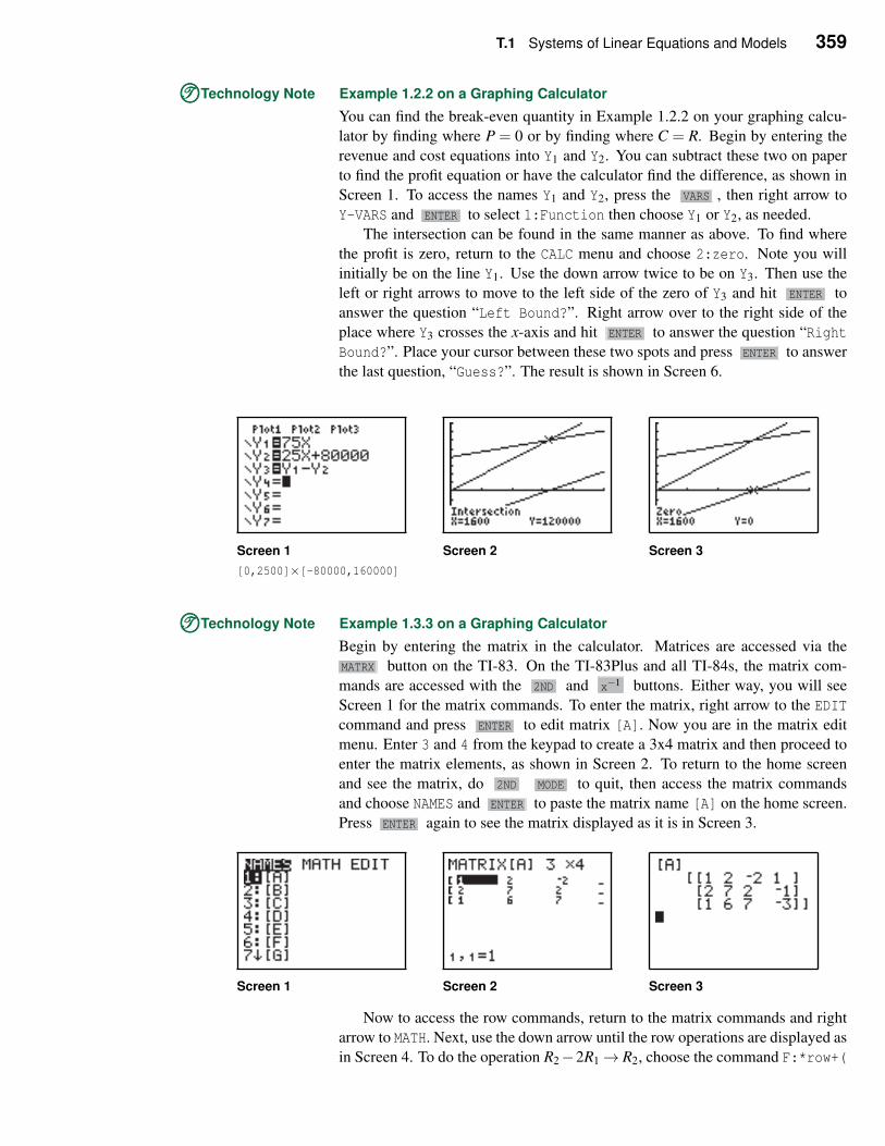
T.1 Systems of Linear Equations and Models 359
TTT©©©Technology Note Example 1.2.2 on a Graphing Calculator
You can find the break-even quantity in Example 1.2.2 on your graphing calcu-
lator by finding where P = 0 or by finding where C = R. Begin by entering the
revenue and cost equations into Y1 and Y2. You can subtract these two on paper
to find the profit equation or have the calculator find the difference, as shown in
Screen 1. To access the names Y1 and Y2, press the VARS , then right arrow to
Y-VARS and ENTER to select 1:Function then choose Y1 or Y2, as needed.
The intersection can be found in the same manner as above. To find where
the profit is zero, return to the CALC menu and choose 2:zero. Note you will
initially be on the line Y1. Use the down arrow twice to be on Y3. Then use the
left or right arrows to move to the left side of the zero of Y3 and hit ENTER to
answer the question “Left Bound?”. Right arrow over to the right side of the
place where Y3 crosses the x-axis and hit ENTER to answer the question “Right
Bound?”. Place your cursor between these two spots and press ENTER to answer
the last question, “Guess?”. The result is shown in Screen 6.
Screen 1
[0,2500]×[-80000,160000]Screen 2 Screen 3
TTT©©©Technology Note Example 1.3.3 on a Graphing Calculator
Begin by entering the matrix in the calculator. Matrices are accessed via the
MATRX button on the TI-83. On the TI-83Plus and all TI-84s, the matrix com-
mands are accessed with the 2ND and x−1 buttons. Either way, you will see
Screen 1 for the matrix commands. To enter the matrix, right arrow to the EDIT
command and press ENTER to edit matrix [A]. Now you are in the matrix edit
menu. Enter 3 and 4 from the keypad to create a 3x4 matrix and then proceed to
enter the matrix elements, as shown in Screen 2. To return to the home screen
and see the matrix, do 2ND MODE to quit, then access the matrix commands
and choose NAMES and ENTER to paste the matrix name [A] on the home screen.
Press ENTER again to see the matrix displayed as it is in Screen 3.
Screen 1 Screen 2 Screen 3
Now to access the row commands, return to the matrix commands and right
arrow to MATH. Next, use the down arrow until the row operations are displayed as
in Screen 4. To do the operation R2−2R1→ R2, choose the command F:*row+(
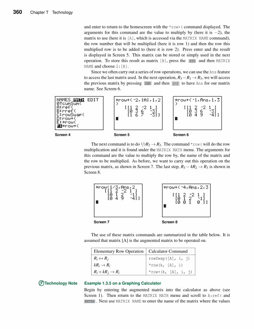
360 Chapter T Technology
and enter to return to the homescreen with the *row+( command displayed. The
arguments for this command are the value to multiply by (here it is −2), the
matrix to use (here it is [A], which is accessed via the MATRIX NAME command),
the row number that will be multiplied (here it is row 1) and then the row this
multiplied row is to be added to (here it is row 2). Press enter and the result
is displayed in Screen 5. This matrix can be stored or simply used in the next
operation. To store this result as matrix [B], press the STO and then MATRIX
NAME and choose 2:[B].
Since we often carry out a series of row operations, we can use the Ans feature
to access the last matrix used. In the next operation, R3−R1→ R3, we will access
the previous matrix by pressing 2ND and then (-) to have Ans for our matrix
name. See Screen 6.
Screen 4 Screen 5 Screen 6
The next command is to do 1/3R2→ R2. The command *row( will do the row
multiplication and it is found under the MATRIX MATH menu. The arguments for
this command are the value to multiply the row by, the name of the matrix and
the row to be multiplied. As before, we want to carry out this operation on the
previous matrix, as shown in Screen 7. The last step, R3−4R2→ R3 is shown in
Screen 8.
Screen 7 Screen 8
The use of these matrix commands are summarized in the table below. It is
assumed that matrix [A] is the augmented matrix to be operated on.
Elementary Row Operation Calculator Command
Ri↔ R j rowSwap([A], i, j)
kRi→ Ri *row(k, [A], i)
Ri + kR j→ Ri *row+(k, [A], i, j)
TTT©©©Technology Note Example 1.3.5 on a Graphing Calculator
Begin by entering the augmented matrix into the calculator as above (see
Screen 1). Then return to the MATRIX MATH menu and scroll to A:ref( and
ENTER . Next use MATRIX NAME to enter the name of the matrix where the values
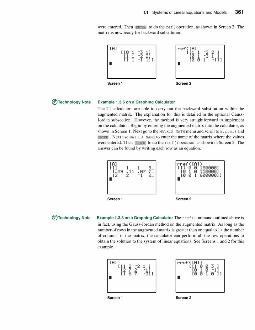
T.1 Systems of Linear Equations and Models 361
were entered. Then ENTER to do the ref( operation, as shown in Screen 2. The
matrix is now ready for backward substitution.
Screen 1 Screen 2
TTT©©©Technology Note Example 1.3.6 on a Graphing Calculator
The TI calculators are able to carry out the backward substitution within the
augmented matrix. The explanation for this is detailed in the optional Gauss-
Jordan subsection. However, the method is very straightforward to implement
on the calculator. Begin by entering the augmented matrix into the calculator, as
shown in Screen 1. Next go to the MATRIX MATH menu and scroll to B:rref( and
ENTER . Next use MATRIX NAME to enter the name of the matrix where the values
were entered. Then ENTER to do the rref( operation, as shown in Screen 2. The
answer can be found by writing each row as an equation.
Screen 1 Screen 2
TTT©©©Technology Note Example 1.3.3 on a Graphing Calculator The rref( command outlined above is
in fact, using the Gauss-Jordan method on the augmented matrix. As long as the
number of rows in the augmented matrix is greater than or equal to 1+ the number
of columns in the matrix, the calculator can perform all the row operations to
obtain the solution to the system of linear equations. See Screens 1 and 2 for this
example.
Screen 1 Screen 2
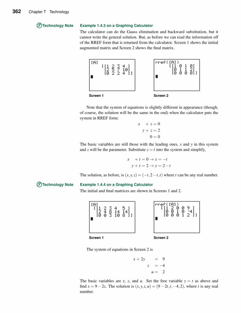
362 Chapter T Technology
TTT©©©Technology Note Example 1.4.3 on a Graphing Calculator
The calculator can do the Gauss elimination and backward substitution, but it
cannot write the general solution. But, as before we can read the information off
of the RREF form that is returned from the calculator. Screen 1 shows the initial
augmented matrix and Screen 2 shows the final matrix.
Screen 1 Screen 2
Note that the system of equations is slightly different in appearance (though,
of course, the solution will be the same in the end) when the calculator puts the
system in RREF form:
x + z = 0
y + z = 2
0 = 0
The basic variables are still those with the leading ones, x and y in this system
and z will be the parameter. Substitute z = t into the system and simplify,
x + t = 0→ x = −t
y + t = 2→ y = 2− t
The solution, as before, is (x,y,z) = (−t,2− t, t) where t can be any real number.
TTT©©©Technology Note Example 1.4.4 on a Graphing Calculator
The initial and final matrices are shown in Screens 1 and 2.
Screen 1 Screen 2
The system of equations in Screen 2 is
x + 2y = 9
z = −4
u = 2
The basic variables are x, z, and u. Set the free variable y = t as above and
find x = 9−2z. The solution is (x,y,z,u) = (9−2t, t,−4,2), where t is any real
number.
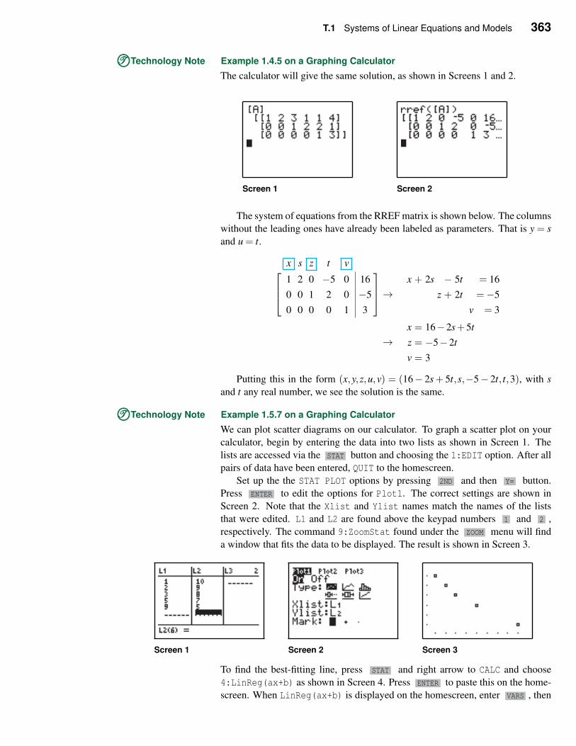
T.1 Systems of Linear Equations and Models 363
TTT©©©Technology Note Example 1.4.5 on a Graphing Calculator
The calculator will give the same solution, as shown in Screens 1 and 2.
Screen 1 Screen 2
The system of equations from the RREF matrix is shown below. The columns
without the leading ones have already been labeled as parameters. That is y = s
and u = t.
x s z t v
1 2 0 −5 0 16
0 0 1 2 0 −5
0 0 0 0 1 3
→
x + 2s − 5t = 16
z + 2t =−5
v = 3
→x = 16−2s+5t
z = −5−2t
v = 3
Putting this in the form (x,y,z,u,v) = (16− 2s+ 5t,s,−5− 2t, t,3), with s
and t any real number, we see the solution is the same.
TTT©©©Technology Note Example 1.5.7 on a Graphing Calculator
We can plot scatter diagrams on our calculator. To graph a scatter plot on your
calculator, begin by entering the data into two lists as shown in Screen 1. The
lists are accessed via the STAT button and choosing the 1:EDIT option. After all
pairs of data have been entered, QUIT to the homescreen.
Set up the the STAT PLOT options by pressing 2ND and then Y= button.
Press ENTER to edit the options for Plot1. The correct settings are shown in
Screen 2. Note that the Xlist and Ylist names match the names of the lists
that were edited. L1 and L2 are found above the keypad numbers 1 and 2 ,
respectively. The command 9:ZoomStat found under the ZOOM menu will find
a window that fits the data to be displayed. The result is shown in Screen 3.
Screen 1 Screen 2 Screen 3
To find the best-fitting line, press STAT and right arrow to CALC and choose
4:LinReg(ax+b) as shown in Screen 4. Press ENTER to paste this on the home-
screen. When LinReg(ax+b) is displayed on the homescreen, enter VARS , then
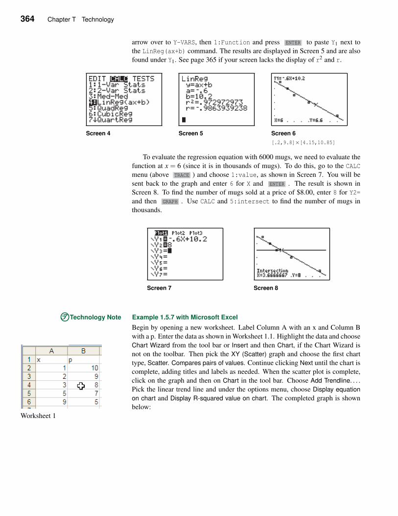
364 Chapter T Technology
arrow over to Y-VARS, then 1:Function and press ENTER to paste Y1 next to
the LinReg(ax+b) command. The results are displayed in Screen 5 and are also
found under Y1. See page 365 if your screen lacks the display of r2 and r.
Screen 4 Screen 5 Screen 6
[.2,9.8]×[4.15,10.85]
To evaluate the regression equation with 6000 mugs, we need to evaluate the
function at x = 6 (since it is in thousands of mugs). To do this, go to the CALC
menu (above TRACE ) and choose 1:value, as shown in Screen 7. You will be
sent back to the graph and enter 6 for X and ENTER . The result is shown in
Screen 8. To find the number of mugs sold at a price of $8.00, enter 8 for Y2=
and then GRAPH . Use CALC and 5:intersect to find the number of mugs in
thousands.
Screen 7 Screen 8
TTT©©©Technology Note Example 1.5.7 with Microsoft Excel
Begin by opening a new worksheet. Label Column A with an x and Column B
with a p. Enter the data as shown in Worksheet 1.1. Highlight the data and choose
Chart Wizard from the tool bar or Insert and then Chart, if the Chart Wizard is
not on the toolbar. Then pick the XY (Scatter) graph and choose the first chart
type, Scatter. Compares pairs of values. Continue clicking Next until the chart is
complete, adding titles and labels as needed. When the scatter plot is complete,
click on the graph and then on Chart in the tool bar. Choose Add Trendline. . . .
Pick the linear trend line and under the options menu, choose Display equation
on chart and Display R-squared value on chart. The completed graph is shown
below:
Worksheet 1
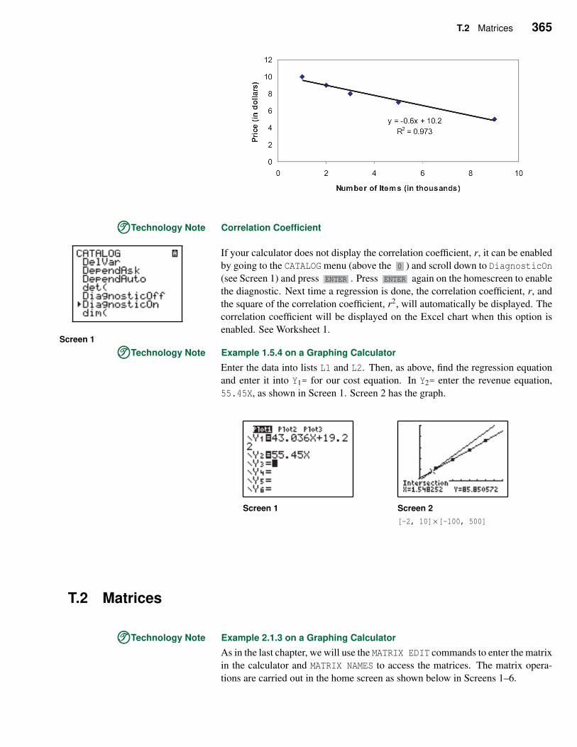
T.2 Matrices 365
TTT©©©Technology Note Correlation Coefficient
If your calculator does not display the correlation coefficient, r, it can be enabled
by going to the CATALOG menu (above the 0 ) and scroll down to DiagnosticOn
(see Screen 1) and press ENTER . Press ENTER again on the homescreen to enable
the diagnostic. Next time a regression is done, the correlation coefficient, r, and
the square of the correlation coefficient, r2, will automatically be displayed. The
Screen 1
correlation coefficient will be displayed on the Excel chart when this option is
enabled. See Worksheet 1.
TTT©©©Technology Note Example 1.5.4 on a Graphing Calculator
Enter the data into lists L1 and L2. Then, as above, find the regression equation
and enter it into Y1= for our cost equation. In Y2= enter the revenue equation,
55.45X, as shown in Screen 1. Screen 2 has the graph.
Screen 1 Screen 2
[-2, 10]×[-100, 500]
T.2 Matrices
TTT©©©Technology Note Example 2.1.3 on a Graphing Calculator
As in the last chapter, we will use the MATRIX EDIT commands to enter the matrix
in the calculator and MATRIX NAMES to access the matrices. The matrix opera-
tions are carried out in the home screen as shown below in Screens 1–6.
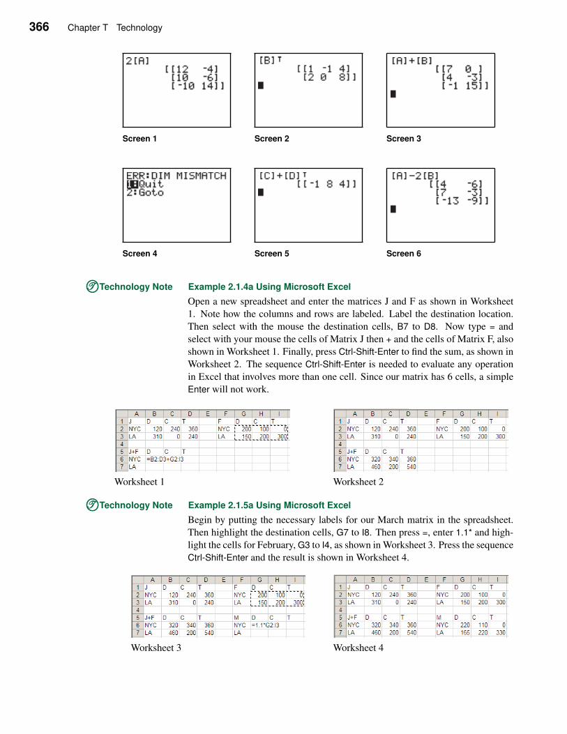
366 Chapter T Technology
Screen 1 Screen 2 Screen 3
Screen 4 Screen 5 Screen 6
TTT©©©Technology Note Example 2.1.4a Using Microsoft Excel
Open a new spreadsheet and enter the matrices J and F as shown in Worksheet
1. Note how the columns and rows are labeled. Label the destination location.
Then select with the mouse the destination cells, B7 to D8. Now type = and
select with your mouse the cells of Matrix J then + and the cells of Matrix F, also
shown in Worksheet 1. Finally, press Ctrl-Shift-Enter to find the sum, as shown in
Worksheet 2. The sequence Ctrl-Shift-Enter is needed to evaluate any operation
in Excel that involves more than one cell. Since our matrix has 6 cells, a simple
Enter will not work.
Worksheet 1 Worksheet 2
TTT©©©Technology Note Example 2.1.5a Using Microsoft Excel
Begin by putting the necessary labels for our March matrix in the spreadsheet.
Then highlight the destination cells, G7 to I8. Then press =, enter 1.1* and high-
light the cells for February, G3 to I4, as shown in Worksheet 3. Press the sequence
Ctrl-Shift-Enter and the result is shown in Worksheet 4.
Worksheet 3 Worksheet 4
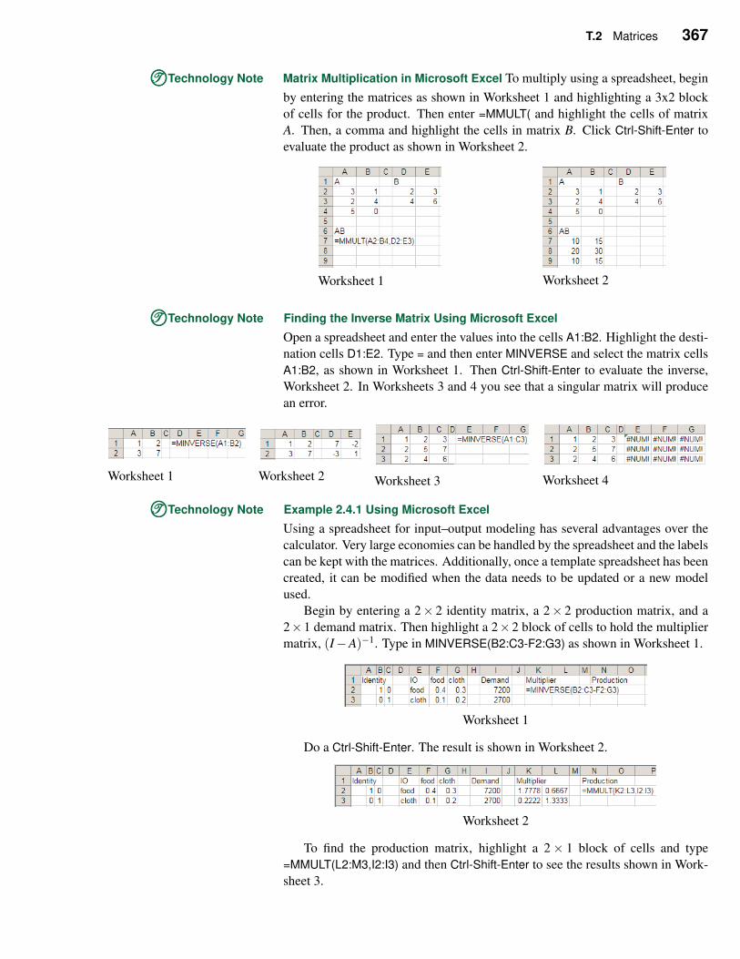
T.2 Matrices 367
TTT©©©Technology Note Matrix Multiplication in Microsoft Excel To multiply using a spreadsheet, begin
by entering the matrices as shown in Worksheet 1 and highlighting a 3x2 block
of cells for the product. Then enter =MMULT( and highlight the cells of matrix
A. Then, a comma and highlight the cells in matrix B. Click Ctrl-Shift-Enter to
evaluate the product as shown in Worksheet 2.
Worksheet 1 Worksheet 2
TTT©©©Technology Note Finding the Inverse Matrix Using Microsoft Excel
Open a spreadsheet and enter the values into the cells A1:B2. Highlight the desti-
nation cells D1:E2. Type = and then enter MINVERSE and select the matrix cells
A1:B2, as shown in Worksheet 1. Then Ctrl-Shift-Enter to evaluate the inverse,
Worksheet 2. In Worksheets 3 and 4 you see that a singular matrix will produce
an error.
Worksheet 1 Worksheet 2 Worksheet 3 Worksheet 4
TTT©©©Technology Note Example 2.4.1 Using Microsoft Excel
Using a spreadsheet for input–output modeling has several advantages over the
calculator. Very large economies can be handled by the spreadsheet and the labels
can be kept with the matrices. Additionally, once a template spreadsheet has been
created, it can be modified when the data needs to be updated or a new model
used.
Begin by entering a 2× 2 identity matrix, a 2× 2 production matrix, and a
2×1 demand matrix. Then highlight a 2×2 block of cells to hold the multiplier
matrix, (I−A)−1. Type in MINVERSE(B2:C3-F2:G3) as shown in Worksheet 1.
Worksheet 1
Do a Ctrl-Shift-Enter. The result is shown in Worksheet 2.
Worksheet 2
To find the production matrix, highlight a 2× 1 block of cells and type
=MMULT(L2:M3,I2:I3) and then Ctrl-Shift-Enter to see the results shown in Work-
sheet 3.
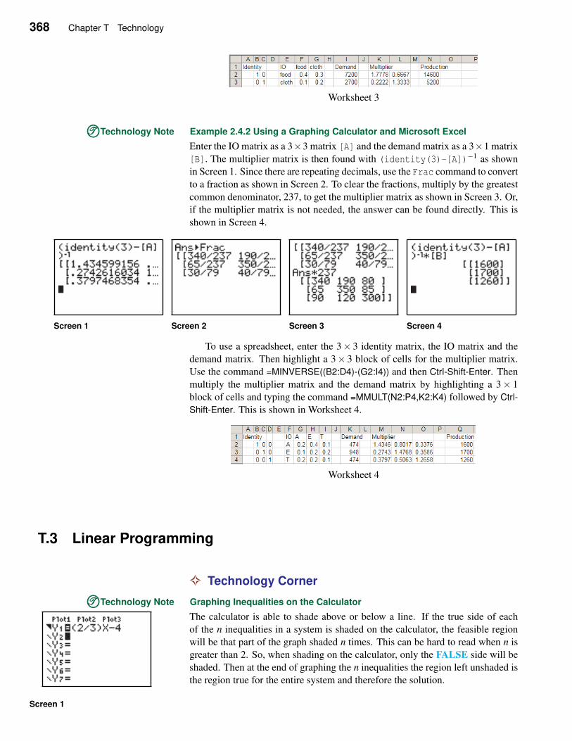
368 Chapter T Technology
Worksheet 3
TTT©©©Technology Note Example 2.4.2 Using a Graphing Calculator and Microsoft Excel
Enter the IO matrix as a 3×3 matrix [A] and the demand matrix as a 3×1 matrix
[B]. The multiplier matrix is then found with (identity(3)-[A])−1 as shown
in Screen 1. Since there are repeating decimals, use the Frac command to convert
to a fraction as shown in Screen 2. To clear the fractions, multiply by the greatest
common denominator, 237, to get the multiplier matrix as shown in Screen 3. Or,
if the multiplier matrix is not needed, the answer can be found directly. This is
shown in Screen 4.
Screen 1 Screen 2 Screen 3 Screen 4
To use a spreadsheet, enter the 3× 3 identity matrix, the IO matrix and the
demand matrix. Then highlight a 3× 3 block of cells for the multiplier matrix.
Use the command =MINVERSE((B2:D4)-(G2:I4)) and then Ctrl-Shift-Enter. Then
multiply the multiplier matrix and the demand matrix by highlighting a 3× 1
block of cells and typing the command =MMULT(N2:P4,K2:K4) followed by Ctrl-
Shift-Enter. This is shown in Worksheet 4.
Worksheet 4
T.3 Linear Programming
✧ Technology Corner
TTT©©©Technology Note Graphing Inequalities on the Calculator
The calculator is able to shade above or below a line. If the true side of each
of the n inequalities in a system is shaded on the calculator, the feasible region
will be that part of the graph shaded n times. This can be hard to read when n is
greater than 2. So, when shading on the calculator, only the FALSE side will be
shaded. Then at the end of graphing the n inequalities the region left unshaded is
the region true for the entire system and therefore the solution.
Screen 1
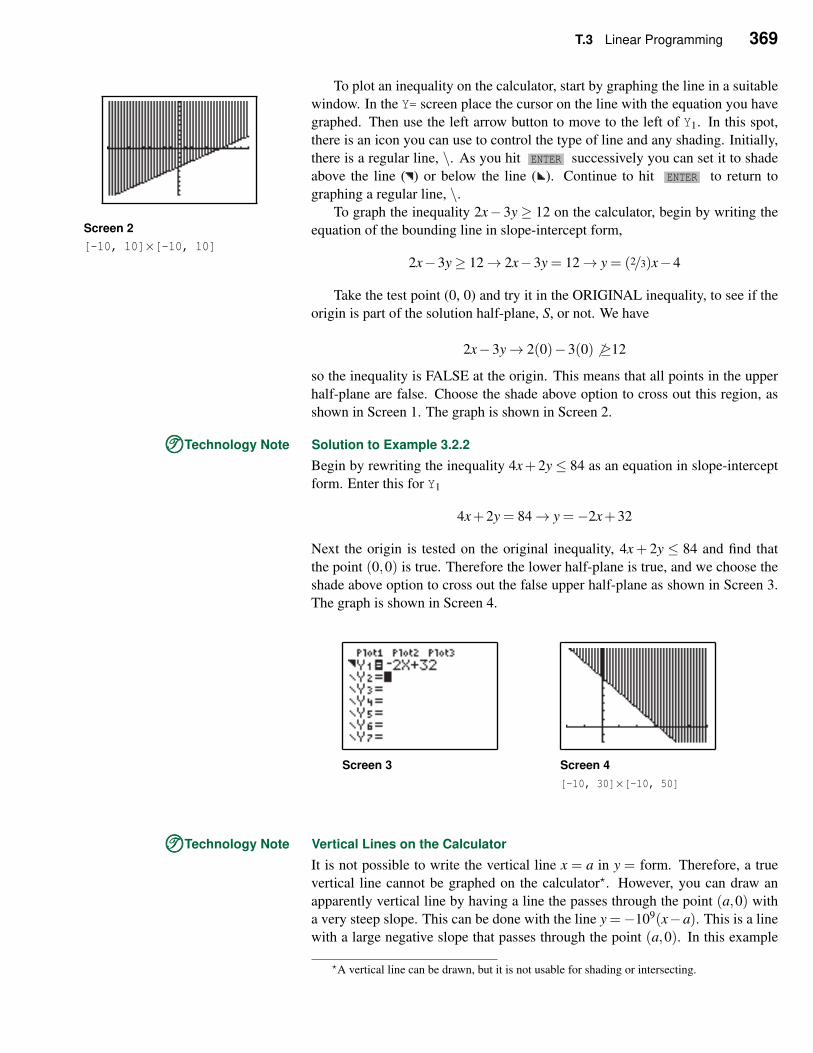
T.3 Linear Programming 369
To plot an inequality on the calculator, start by graphing the line in a suitable
window. In the Y= screen place the cursor on the line with the equation you have
graphed. Then use the left arrow button to move to the left of Y1. In this spot,
there is an icon you can use to control the type of line and any shading. Initially,
there is a regular line, \. As you hit ENTER successively you can set it to shade
above the line ( ) or below the line ( ). Continue to hit ENTER to return to
graphing a regular line, \.
Screen 2
[-10, 10]×[-10, 10]
To graph the inequality 2x− 3y ≥ 12 on the calculator, begin by writing the
equation of the bounding line in slope-intercept form,
2x−3y≥ 12→ 2x−3y = 12→ y = (2/3)x−4
Take the test point (0, 0) and try it in the ORIGINAL inequality, to see if the
origin is part of the solution half-plane, S, or not. We have
2x−3y→ 2(0)−3(0) 6 ≥12
so the inequality is FALSE at the origin. This means that all points in the upper
half-plane are false. Choose the shade above option to cross out this region, as
shown in Screen 1. The graph is shown in Screen 2.
TTT©©©Technology Note Solution to Example 3.2.2
Begin by rewriting the inequality 4x+ 2y ≤ 84 as an equation in slope-intercept
form. Enter this for Y1
4x+2y = 84→ y =−2x+32
Next the origin is tested on the original inequality, 4x+ 2y ≤ 84 and find that
the point (0,0) is true. Therefore the lower half-plane is true, and we choose the
shade above option to cross out the false upper half-plane as shown in Screen 3.
The graph is shown in Screen 4.
Screen 3 Screen 4
[-10, 30]×[-10, 50]
TTT©©©Technology Note Vertical Lines on the Calculator
It is not possible to write the vertical line x = a in y = form. Therefore, a true
vertical line cannot be graphed on the calculator⋆. However, you can draw an
apparently vertical line by having a line the passes through the point (a,0) with
a very steep slope. This can be done with the line y =−109(x−a). This is a line
with a large negative slope that passes through the point (a,0). In this example
⋆A vertical line can be drawn, but it is not usable for shading or intersecting.
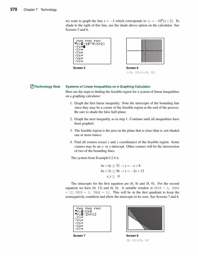
370 Chapter T Technology
we want to graph the line x = −2 which corresponds to Y1 = −109(x+ 2). To
shade to the right of this line, use the shade above option on the calculator. See
Screens 5 and 6.
Screen 5 Screen 6
[-10, 10]×[-10, 10]
TTT©©©Technology Note Systems of Linear Inequalities on a Graphing Calculator
Here are the steps to finding the feasible region for a system of linear inequalities
on a graphing calculator:
1. Graph the first linear inequality. Note the intercepts of the bounding line
since they may be a corner of the feasible region at the end of the process.
Be sure to shade the false half-plane.
2. Graph the next inequality as in step 1. Continue until all inequalities have
been graphed.
3. The feasible region is the area on the plane that is clear (that is, not shaded
one or more times).
4. Find all corners (exact x and y coordinates) of the feasible region. Some
corners may be an x- or y-intercept. Other corners will be the intersection
of two of the bounding lines.
The system from Example3.2.4 is
4x+4y ≤ 32→ y =−x+8
6x+3y ≤ 36→ y =−2x+12
x,y ≥ 0
The intercepts for the first equation are (0, 8) and (8, 0). For the second
equation we have (0, 12) and (6, 0). A suitable window is XMIN = 0, XMAX
= 12, YMIN = 0, YMAX = 12. This will be in the first quadrant to keep the
nonnegativity condition and allow the intercepts to be seen. See Screens 7 and 8.
Screen 7 Screen 8
[0, 12]×[0, 12]
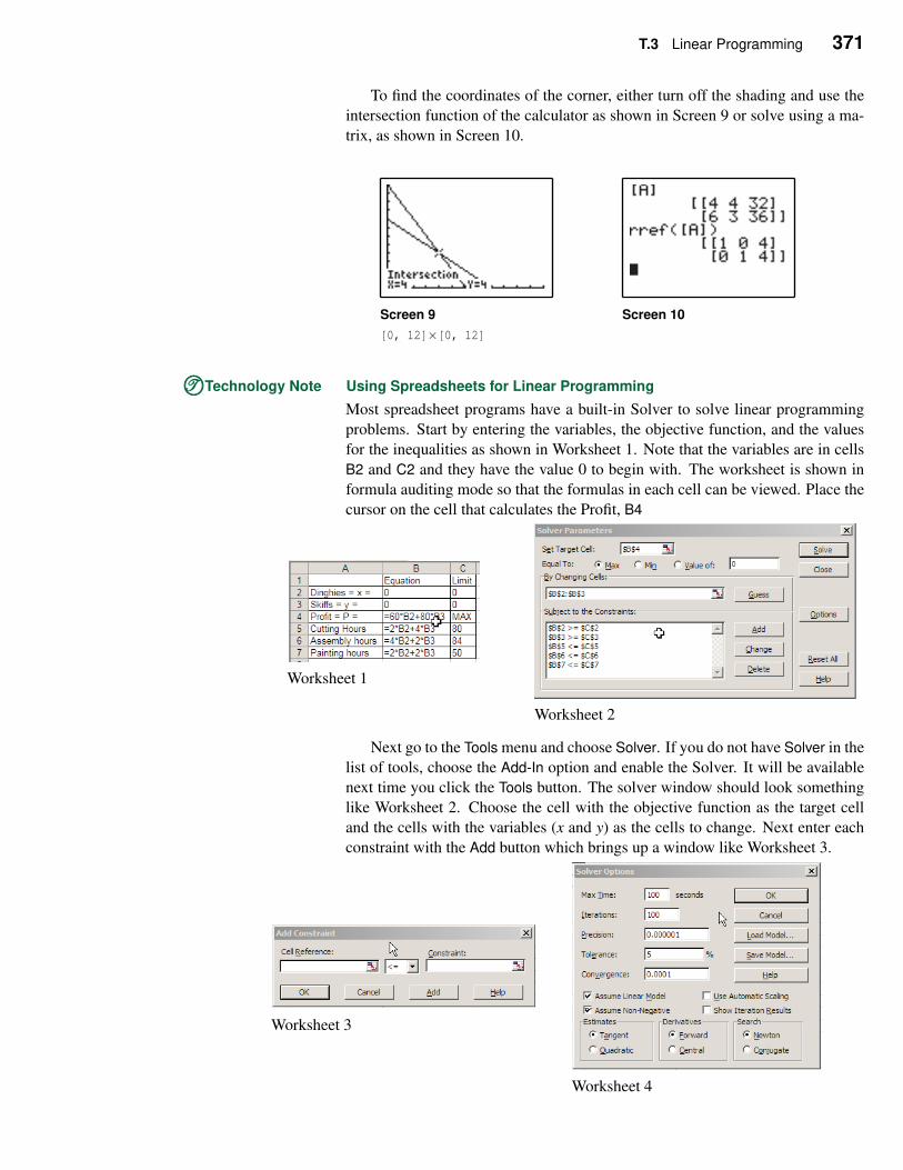
T.3 Linear Programming 371
To find the coordinates of the corner, either turn off the shading and use the
intersection function of the calculator as shown in Screen 9 or solve using a ma-
trix, as shown in Screen 10.
Screen 9
[0, 12]×[0, 12]
Screen 10
TTT©©©Technology Note Using Spreadsheets for Linear Programming
Most spreadsheet programs have a built-in Solver to solve linear programming
problems. Start by entering the variables, the objective function, and the values
for the inequalities as shown in Worksheet 1. Note that the variables are in cells
B2 and C2 and they have the value 0 to begin with. The worksheet is shown in
formula auditing mode so that the formulas in each cell can be viewed. Place the
cursor on the cell that calculates the Profit, B4
Worksheet 1
Worksheet 2
Next go to the Tools menu and choose Solver. If you do not have Solver in the
list of tools, choose the Add-In option and enable the Solver. It will be available
next time you click the Tools button. The solver window should look something
like Worksheet 2. Choose the cell with the objective function as the target cell
and the cells with the variables (x and y) as the cells to change. Next enter each
constraint with the Add button which brings up a window like Worksheet 3.
Worksheet 3
Worksheet 4
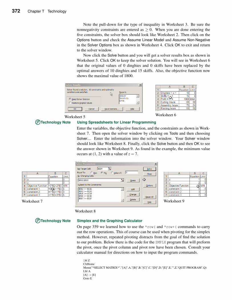
372 Chapter T Technology
Note the pull-down for the type of inequality in Worksheet 3. Be sure the
nonnegativity constraints are entered as ≥ 0. When you are done entering the
five constraints, the solver box should look like Worksheet 2. Then click on the
Options button and check the Assume Linear Model and Assume Non-Negative
in the Solver Options box as shown in Worksheet 4. Click OK to exit and return
to the solver window.
Now click the Solve button and you will get a solver results box as shown in
Worksheet 5. Click OK to keep the solver solution. You will see in Worksheet 6
that the original values of 0 dinghies and 0 skiffs have been replaced by the
optimal answers of 10 dinghies and 15 skiffs. Also, the objective function now
shows the maximal value of 1800.
Worksheet 5 Worksheet 6
TTT©©©Technology Note Using Spreadsheets for Linear Programming
Enter the variables, the objective function, and the constraints as shown in Work-
sheet 7. Then open the solver window by clicking on Tools and then choosing
Solver.... Enter the information into the solver window. Your Solver window
should look like Worksheet 8. Finally, click the Solve button and then OK to see
the answer shown in Worksheet 9. As found in the example, the minimum value
occurs at (1, 2) with a value of z = 7.
Worksheet 7
Worksheet 8
Worksheet 9
TTT©©©Technology Note Simplex and the Graphing Calculator
On page 359 we learned how to use the *row( and *row+( commands to carry
out the row operations. This of course can be used when pivoting for the simplex
method. However, repeated pivoting distracts from the goal of find the solution
to our problem. Below there is the code for the SMPLX program that will preform
the pivot, once the pivot column and pivot row have been chosen. Consult your
calculator manual for directions on how to input the program commands.
Lbl Z
ClrHome
Menu("*SELECT MATRIX*","[A]",A,"[B]",B,"[C]",C,"[D]",D,"[E]",E,"",Z,"QUIT PROGRAM",Q)
Lbl A
[A]→ [E]
Goto E
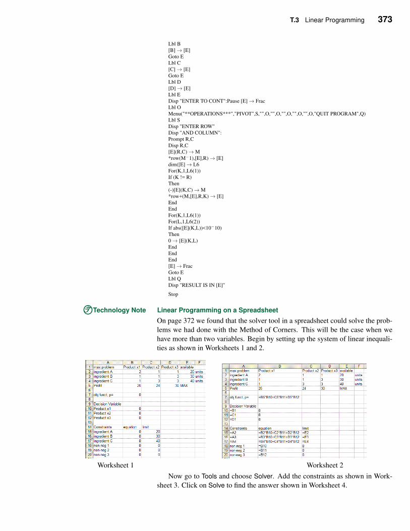
T.3 Linear Programming 373
Lbl B
[B]→ [E]
Goto E
Lbl C
[C]→ [E]
Goto E
Lbl D
[D]→ [E]
Lbl E
Disp "ENTER TO CONT":Pause [E]→ Frac
Lbl O
Menu("**OPERATIONS***","PIVOT",S,"",O,"",O,"",O,"",O,"",O,"QUIT PROGRAM",Q)
Lbl S
Disp "ENTER ROW"
Disp "AND COLUMN":
Prompt R,C
Disp R,C
[E](R,C)→M
*row(M−1),[E],R)→ [E]
dim([E]→ L6
For(K,1,L6(1))
If (K != R)
Then
(-)[E](K,C)→M
*row+(M,[E],R,K)→ [E]
End
End
For(K,1,L6(1))
For(L,1,L6(2))
If abs([E](K,L))<10−10)
Then
0→ [E](K,L)
End
End
End
[E]→ Frac
Goto E
Lbl Q
Disp "RESULT IS IN [E]"
Stop
TTT©©©Technology Note Linear Programming on a Spreadsheet
On page 372 we found that the solver tool in a spreadsheet could solve the prob-
lems we had done with the Method of Corners. This will be the case when we
have more than two variables. Begin by setting up the system of linear inequali-
ties as shown in Worksheets 1 and 2.
Worksheet 1 Worksheet 2
Now go to Tools and choose Solver. Add the constraints as shown in Work-
sheet 3. Click on Solve to find the answer shown in Worksheet 4.
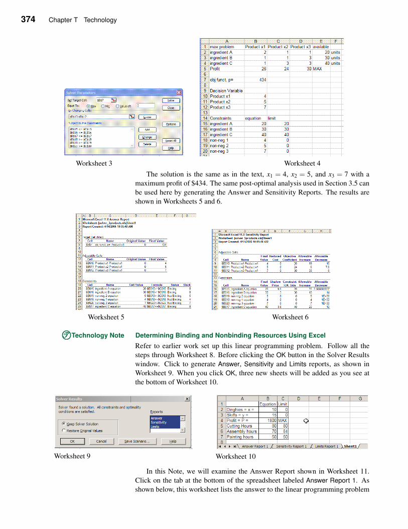
374 Chapter T Technology
Worksheet 3 Worksheet 4
The solution is the same as in the text, x1 = 4, x2 = 5, and x3 = 7 with a
maximum profit of $434. The same post-optimal analysis used in Section 3.5 can
be used here by generating the Answer and Sensitivity Reports. The results are
shown in Worksheets 5 and 6.
Worksheet 5 Worksheet 6
TTT©©©Technology Note Determining Binding and Nonbinding Resources Using Excel
Refer to earlier work set up this linear programming problem. Follow all the
steps through Worksheet 8. Before clicking the OK button in the Solver Results
window. Click to generate Answer, Sensitivity and Limits reports, as shown in
Worksheet 9. When you click OK, three new sheets will be added as you see at
the bottom of Worksheet 10.
Worksheet 9 Worksheet 10
In this Note, we will examine the Answer Report shown in Worksheet 11.
Click on the tab at the bottom of the spreadsheet labeled Answer Report 1. As
shown below, this worksheet lists the answer to the linear programming problem
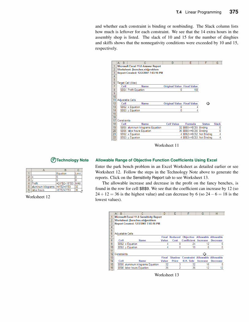
T.4 Linear Programming 375
and whether each constraint is binding or nonbinding. The Slack column lists
how much is leftover for each constraint. We see that the 14 extra hours in the
assembly shop is listed. The slack of 10 and 15 for the number of dinghies
and skiffs shows that the nonnegativity conditions were exceeded by 10 and 15,
respectively.
Worksheet 11
TTT©©©Technology Note Allowable Range of Objective Function Coefficients Using Excel
Enter the park bench problem in an Excel Worksheet as detailed earlier or see
Worksheet 12. Follow the steps in the Technology Note above to generate the
reports. Click on the Sensitivity Report tab to see Worksheet 13.
The allowable increase and decrease in the profit on the fancy benches, is
Worksheet 12
found in the row for cell $B$9. We see that the coefficient can increase by 12 (so
24+ 12 = 36 is the highest value) and can decrease by 6 (so 24− 6 = 18 is the
lowest values).
Worksheet 13
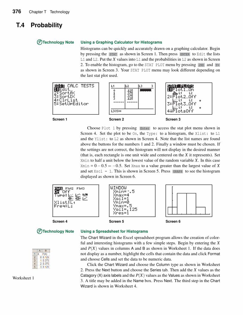
376 Chapter T Technology
T.4 Probability
TTT©©©Technology Note Using a Graphing Calculator for Histograms
Histograms can be quickly and accurately drawn on a graphing calculator. Begin
by pressing the STAT as shown in Screen 1. Then press ENTER to Edit the lists
L1 and L2. Put the X values into L1 and the probabilities in L2 as shown in Screen
2. To enable the histogram, go to the STAT PLOT menu by pressing 2ND and Y=
as shown in Screen 3. Your STAT PLOT menu may look different depending on
the last stat plot used.
Screen 1 Screen 2 Screen 3
Choose Plot 1 by pressing Enter to access the stat plot menu shown in
Screen 4. Set the plot to be On, the Type: to a histogram, the Xlist: to L1
and the Ylist: to L2 as shown in Screen 4. Note that the list names are found
above the buttons for the numbers 1 and 2. Finally a window must be chosen. If
the settings are not correct, the histogram will not display in the desired manner
(that is, each rectangle is one unit wide and centered on the X it represents). Set
Xmin to half a unit below the lowest value of the random variable X . In this case
Xmin = 0− 0.5 = −0.5. Set Xmax to a value greater than the largest value of X
and set Xscl = 1. This is shown in Screen 5. Press GRAPH to see the histogram
displayed as shown in Screen 6.
Screen 4 Screen 5 Screen 6
TTT©©©Technology Note Using a Spreadsheet for Histograms
The Chart Wizard in the Excel spreadsheet program allows the creation of color-
ful and interesting histograms with a few simple steps. Begin by entering the X
and P(X) values in columns A and B as shown in Worksheet 1. If the data does
Worksheet 1
not display as a number, highlight the cells that contain the data and click Format
and choose Cells and set the data to be numeric data.
Click the Chart Wizard and choose the Column type as shown in Worksheet
2. Press the Next button and choose the Series tab. Then add the X values as the
Catagory (X) axis labels and the P(X) values as the Values as shown in Worksheet
3. A title may be added in the Name box. Press Next. The third step in the Chart
Wizard is shown in Worksheet 4.
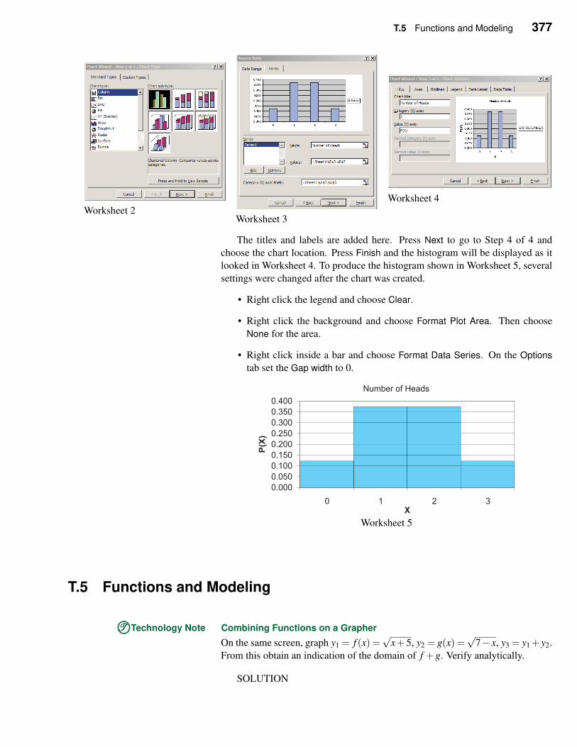
T.5 Functions and Modeling 377
Worksheet 2Worksheet 3
Worksheet 4
The titles and labels are added here. Press Next to go to Step 4 of 4 and
choose the chart location. Press Finish and the histogram will be displayed as it
looked in Worksheet 4. To produce the histogram shown in Worksheet 5, several
settings were changed after the chart was created.
• Right click the legend and choose Clear.
• Right click the background and choose Format Plot Area. Then choose
None for the area.
• Right click inside a bar and choose Format Data Series. On the Options
tab set the Gap width to 0.
Number of Heads
0.000
0.050
0.100
0.150
0.200
0.250
0.300
0.350
0.400
0 1 2 3X
P(X
)
Worksheet 5
T.5 Functions and Modeling
TTT©©©Technology Note Combining Functions on a Grapher
On the same screen, graph y1 = f (x) =√
x+5, y2 = g(x) =√
7− x, y3 = y1+y2.
From this obtain an indication of the domain of f +g. Verify analytically.
SOLUTION
378 Chapter T Technology
The graphs are shown in Screen 1.6. Notice how the graph gives us an indi-
cation of the domain of f +g. The domain appears to be [−5,7]. The domain of
f is [−5,∞), and the domain of g is (−∞,7]. Thus the domain of f +g is [−5,7].
⌈ EXPLORATIONS⌋ keep these things?
Exploration 1 Profit
We have that P(x) = R(x)−C(x), where P(x) is profit, R(x) is revenue, and C(x)is cost. Graph on the same screen y1 = R(x) = 12x− x2, y2 = C(x) = 5x+ 4,
y3 = y1− y2, and y4 = P(x) = −x2 +7x−4. What happened to the graph of the
fourth function? Does this indicate that y3 = y4?
Exploration 2 Compositions on Your Grapher
(a) Let y1 = f (x) =√
x, y2 = g(x) = 25− x2, y3 =√
y2, and y4 = 25− y21. Does
y3 correspond to f ◦g or g◦ f ? What about y4?
(b) Confirm your conjectures by graphing y3 and either y = ( f ◦ g)(x) or
y = (g◦ f )(x) together on the same screen. Do the same with y4.
Exploration 3 The Domain of the Composite Function
Confirm Example 3 on your grapher by graphing y = (√
x)2 +5.
⌈ EXPLORATIONS⌋
Exploration 1 Evaluating l(x)
Use a computer or graphing calculator to solve for x to three decimal places in
the equation 2 = 10x. (One way to do this graphically is to find the intersection
of the two graphs of y = 2 and y = 10x.) Check your answer.
Exploration 2 Determining Equalities by Graphing
Decide whether any of the following equations is true by finding the graph of
each side of each equation in the same window.
(a) log10(x+3) = log10 x+ log10 3
(b) log10 x2 = (log10 x)2
(c) log10
x
2=
log10 x
log10 2
Exploration 3 No Analytic Solution
An equation with exponents cannot always be solved by taking logarithms. For
example, the equation 1+ x = 5x cannot be solved by taking logarithms. Try it!
Use your computer or graphing calculator to approximate all solutions.
Enrichment. You may wish to consider modeling half-life in radioactive decay
found in the Enrichment material.
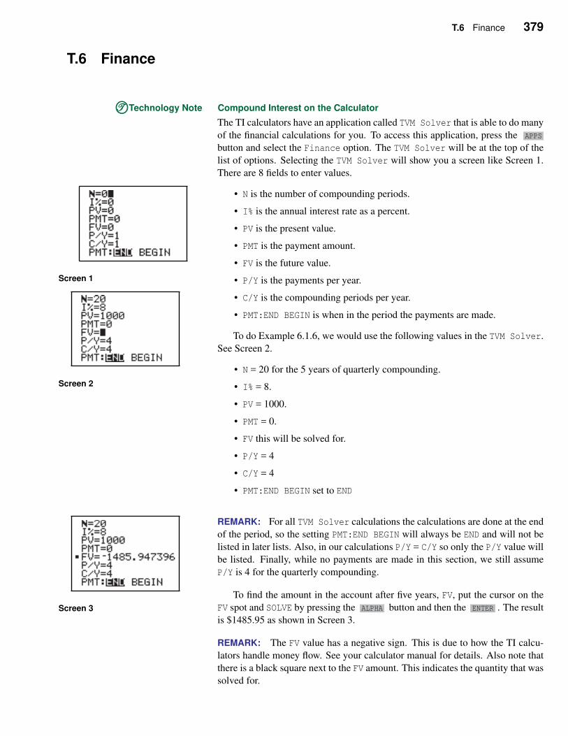
T.6 Finance 379
T.6 Finance
TTT©©©Technology Note Compound Interest on the Calculator
The TI calculators have an application called TVM Solver that is able to do many
of the financial calculations for you. To access this application, press the APPS
button and select the Finance option. The TVM Solver will be at the top of the
list of options. Selecting the TVM Solver will show you a screen like Screen 1.
There are 8 fields to enter values.
Screen 1
• N is the number of compounding periods.
• I% is the annual interest rate as a percent.
• PV is the present value.
• PMT is the payment amount.
• FV is the future value.
• P/Y is the payments per year.
• C/Y is the compounding periods per year.
• PMT:END BEGIN is when in the period the payments are made.
To do Example 6.1.6, we would use the following values in the TVM Solver.
See Screen 2.
Screen 2
• N = 20 for the 5 years of quarterly compounding.
• I% = 8.
• PV = 1000.
• PMT = 0.
• FV this will be solved for.
• P/Y = 4
• C/Y = 4
• PMT:END BEGIN set to END
REMARK: For all TVM Solver calculations the calculations are done at the end
of the period, so the setting PMT:END BEGIN will always be END and will not be
listed in later lists. Also, in our calculations P/Y = C/Y so only the P/Y value will
be listed. Finally, while no payments are made in this section, we still assume
P/Y is 4 for the quarterly compounding.
Screen 3
To find the amount in the account after five years, FV, put the cursor on the
FV spot and SOLVE by pressing the ALPHA button and then the ENTER . The result
is $1485.95 as shown in Screen 3.
REMARK: The FV value has a negative sign. This is due to how the TI calcu-
lators handle money flow. See your calculator manual for details. Also note that
there is a black square next to the FV amount. This indicates the quantity that was
solved for.
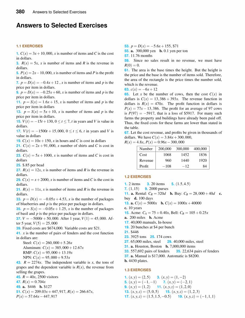
380 Answers to Selected Exercises
Answers to Selected Exercises
1.1 EXERCISES
1. C(x) = 3x+10,000, x is number of items and C is the cost
in dollars.
3. R(x) = 5x, x is number of items and R is the revenue in
dollars.
5. P(x) = 2x−10,000, x is number of items and P is the profit
in dollars.
7. p = D(x) =−0.4x+12 , x is number of items and p is the
price per item in dollars.
9. p = D(x) =−0.25x+60, x is number of items and p is the
price per item in dollars.
11. p = S(x) = 1.6x+ 15, x is number of items and p is the
price per item in dollars
13. p = S(x) = 5x+ 10, x is number of items and p is the
price per item in dollars.
15. V (t) =−15t +130, 0≤ t ≤ 7, t in years and V is value in
dollars.
17. V (t) = −1500t + 15,000, 0 ≤ t ≤ 6, t in years and V is
value in dollars
19. C(x) = 10x+150, x in hours and C is cost in dollars
21. C(x) = 2x+ 91,000, x number of shirts and C is cost in
dollars.
23. C(x) = 5x+ 1000, x is number of items and C is cost in
dollars
25. $.85 per bead
27. R(x) = 12x, x is number of items and R is the revenue in
dollars.
29. C(x) = x+2000, x is number of items and C is the cost in
dollars.
31. R(x) = 11x, x is number of items and R is the revenue in
dollars.
33. p = D(x) = −0.05x+ 4.53, x is the number of packages
of blueberries and p is the price per package in dollars.
35. p = S(x) = −0.05x+ 1.25, x is the number of packages
of basil and p is the price per package in dollars.
37. V =−5000t +50,000. After 1 year, V (1) = 45,000. Af-
ter 5 year, V (5) = 25,000
39. Fixed costs are $674,000. Variable costs are $21.
41. x is the number of pairs of fenders and the cost function
in dollars are:
Steel: C(x) = 260,000+5.26x
Aluminum: C(x) = 385,000+12.67x
RMP: C(x) = 95,000+13.19x
NPN: C(x) = 95,000+9.53x
43. R = 2274x. The independent variable is x, the tons of
grapes and the dependent variable is R(x), the revenue from
selling the grapes.
45. R = 40x, 2500 visitors
47. R(x) = 0.704x
49. a. $446 b. $127
51. C(x) = 209.03x+447,917, R(x) = 266.67x,
P(x) = 57.64x−447,917
53. p = D(x) =−5.6x+155, $71
55. a. 300,000 yen b. 0.1 yen per ton
57. 11.76 months
59. Since no sales result in no revenue, we must have
R(0) = 0.
61. The area is the base times the height. But the height is
the price and the base is the number of items sold. Therefore,
the area of the rectangle is the price times the number sold,
which is the revenue.
63. c(x) =−6x+12
65. Let x be the number of cows, then the cost C(x) in
dollars is C(x) = 13,386 + 393x. The revenue function in
dollars is R(x) = 470x. The profit function in dollars is
P(x) = 77x− 13,386. The profit for an average of 97 cows
is P(97) = −5917, that is a loss of $5917. For many such
farms the property and buildings have already been paid off.
Thus, the fixed costs for these farms are lower than stated in
the table.
67. Let the cost revenue, and profits be given in thousands of
dollars. We have C(x) = 3.84x+300,000,
R(x) = 4.8x, P(x) = 0.96x−300,000
Number 200,000 300,000 400,000
Cost 1068 1452 1836
Revenue 960 1440 1920
Profit −108 −12 84
1.2 EXERCISES
1. 2 items 3. 20 items 5. (1.5,4.5)7. (1,15) 9. 2000 purses
11. a. Rental: CR = 320d b. Buy: CB = 28,000+40d c.
buy d. 100 days
13. a. C(x) = 5000x b. C(x) = 1000x+40000
c. 10 years
15. Acme: CA = 75+0.40x, Bell: CB = 105+0.25x
a. 200 miles b. Acme
17. 40,000 manuals, In-house
19. 20 bunches at $4 per bunch
21. $446
23. 3925 tons 25. 174 cows
27. 65,000 miles, steel 29. 40,000 miles, steel
31. a. Houston, Boston b. 7,000,000 items
33. 557,692 pairs of fenders 35. 22,634 pairs of fenders
37. a. Manual is $17,000. Automatic is $8200.
b. 4430 plates.
1.3 EXERCISES
1. (x,y) = (2,5) 3. (x,y) = (1,−2)5. (x,y) = (−1,−1) 7. (x,y) = (−2,1)9. (x,y) = (1,2) 11. (x,y,z) = (1,2,0)13. (x,y,z) = (5,0,5) 15. (x,y,z) = (1,2,3)17. (x,y,z) = (1.5,1.5,−0.5) 19. (x,y,z) = (−1,1,1)
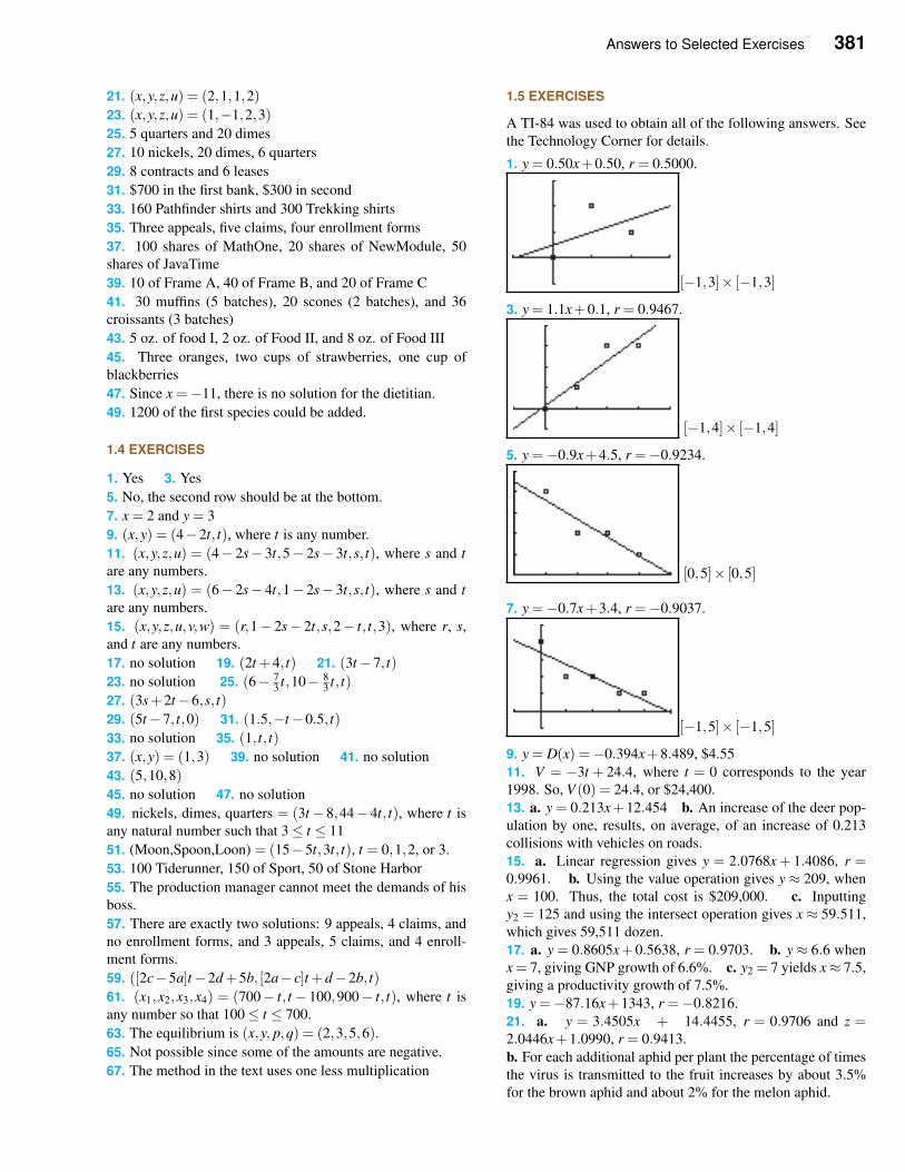
Answers to Selected Exercises 381
21. (x,y,z,u) = (2,1,1,2)
23. (x,y,z,u) = (1,−1,2,3)
25. 5 quarters and 20 dimes
27. 10 nickels, 20 dimes, 6 quarters
29. 8 contracts and 6 leases
31. $700 in the first bank, $300 in second
33. 160 Pathfinder shirts and 300 Trekking shirts
35. Three appeals, five claims, four enrollment forms
37. 100 shares of MathOne, 20 shares of NewModule, 50
shares of JavaTime
39. 10 of Frame A, 40 of Frame B, and 20 of Frame C
41. 30 muffins (5 batches), 20 scones (2 batches), and 36
croissants (3 batches)
43. 5 oz. of food I, 2 oz. of Food II, and 8 oz. of Food III
45. Three oranges, two cups of strawberries, one cup of
blackberries
47. Since x =−11, there is no solution for the dietitian.
49. 1200 of the first species could be added.
1.4 EXERCISES
1. Yes 3. Yes
5. No, the second row should be at the bottom.
7. x = 2 and y = 3
9. (x,y) = (4−2t, t), where t is any number.
11. (x,y,z,u) = (4− 2s− 3t,5− 2s− 3t,s, t), where s and t
are any numbers.
13. (x,y,z,u) = (6− 2s− 4t,1− 2s− 3t,s, t), where s and t
are any numbers.
15. (x,y,z,u,v,w) = (r,1− 2s− 2t,s,2− t, t,3), where r, s,
and t are any numbers.
17. no solution 19. (2t +4, t) 21. (3t−7, t)
23. no solution 25. (6− 73 t,10− 8
3 t, t)
27. (3s+2t−6,s, t)
29. (5t−7, t,0) 31. (1.5,−t−0.5, t)
33. no solution 35. (1, t, t)
37. (x,y) = (1,3) 39. no solution 41. no solution
43. (5,10,8)
45. no solution 47. no solution
49. nickels, dimes, quarters = (3t− 8,44− 4t, t), where t is
any natural number such that 3≤ t ≤ 11
51. (Moon,Spoon,Loon) = (15−5t,3t, t), t = 0,1,2, or 3.
53. 100 Tiderunner, 150 of Sport, 50 of Stone Harbor
55. The production manager cannot meet the demands of his
boss.
57. There are exactly two solutions: 9 appeals, 4 claims, and
no enrollment forms, and 3 appeals, 5 claims, and 4 enroll-
ment forms.
59. ([2c−5a]t−2d +5b, [2a− c]t +d−2b, t)
61. (x1,x2,x3,x4) = (700− t, t − 100,900− t, t), where t is
any number so that 100≤ t ≤ 700.
63. The equilibrium is (x,y, p,q) = (2,3,5,6).
65. Not possible since some of the amounts are negative.
67. The method in the text uses one less multiplication
1.5 EXERCISES
A TI-84 was used to obtain all of the following answers. See
the Technology Corner for details.
1. y = 0.50x+0.50, r = 0.5000.
[−1,3]× [−1,3]
3. y = 1.1x+0.1, r = 0.9467.
[−1,4]× [−1,4]
5. y =−0.9x+4.5, r =−0.9234.
[0,5]× [0,5]
7. y =−0.7x+3.4, r =−0.9037.
[−1,5]× [−1,5]
9. y = D(x) =−0.394x+8.489, $4.55
11. V = −3t + 24.4, where t = 0 corresponds to the year
1998. So, V (0) = 24.4, or $24,400.
13. a. y = 0.213x+12.454 b. An increase of the deer pop-
ulation by one, results, on average, of an increase of 0.213
collisions with vehicles on roads.
15. a. Linear regression gives y = 2.0768x + 1.4086, r =0.9961. b. Using the value operation gives y ≈ 209, when
x = 100. Thus, the total cost is $209,000. c. Inputting
y2 = 125 and using the intersect operation gives x ≈ 59.511,
which gives 59,511 dozen.
17. a. y = 0.8605x+0.5638, r = 0.9703. b. y ≈ 6.6 when
x = 7, giving GNP growth of 6.6%. c. y2 = 7 yields x≈ 7.5,
giving a productivity growth of 7.5%.
19. y =−87.16x+1343, r =−0.8216.
21. a. y = 3.4505x + 14.4455, r = 0.9706 and z =2.0446x+1.0990, r = 0.9413.
b. For each additional aphid per plant the percentage of times
the virus is transmitted to the fruit increases by about 3.5%
for the brown aphid and about 2% for the melon aphid.

382 Answers to Selected Exercises
c. The brown aphid is more destructive since the brown aphid
transmits the virus more often than the melon aphid.
23. a. y = 1.75x+0.140, x = 0 corresponds to the year 2000.
b. 2.59 c. r = 0.9944
25. a. y = 0.35x+ 67.29, x = 0 corresponds the year 2000
b. 69.4% c. r = 0.9737
27. a. y = 411.9x+ 5359.1, x = 1 corresponds for the year
1990 b. 12,361.4 c. r = 0.9984
29. a. y = 100.5x+ 1609.8, x = 1 corresponds to the year
2000 b. 2313.3 c. r = 0.9987
31. a. y = 0.63x+ 60.1, x = 1 corresponds to the year 1990
b. 70.81 c. r = 0.9559
REVIEW EXERCISES
1. C = 2000+ 6x 2. R = 10x 3. P = 4x− 2000, 500
4. 150
5. 1000 6. p =−0.000005x+1.5 7. 12,000
8. P = 12,000t−70,000 9. P = 2000t−20,000
10. a. CR = 150x b. CO = 1400+10x c. He should buy.
d. 10 days
11. (x,y) = (1,2) 12. no solution
13. (x,y) = (1−3t, t) 14. (x,y) = (3,4)
15. (x,y,z) = (1.6−0.2t,0.4t +0.8, t)
16. (x,y,z) = (10− t, t,0) 17. (x,y,z) = (1,3,1)
18. (x,y,z) = (2t−2,7−3t, t)
19. (3 par, 4 par, 5 par) = (t +1,8−2t, t), 0≤ t ≤ 4
20. Seven standard sweepers, five deluxe sweepers
21. 8 of the first and 6 of the second
22. 20 ham specials, 30 beef specials
23. 90 liters of first solution, 60 of second, 150 of third
24. Plants 1, 2, and 3 should produce 100, 200, and 50, re-
spectively.
25. y = (5x+1)/7
26. a. y = 4x+ 45, x = 1 corresponds to the year 1999 b.
77% c. r = 0.9759
2.1 EXERCISES
1. 4×2 3. 1×2 5. 1 7. 8 9. −2 11. 6
13. 2 15. A =
[
5 5 5
5 5 5
]
17.
1 0 0
0 1 0
0 0 1
19.
0 0 0
0 0 0
0 0 0
21. x = 3, y = 0, z = 4
23.
4 5
1 10
−3 10
5 6
25.
[
0 6]
27.
2 −3
−5 −2
3 −4
−1 10
29.
[
−2 −2]
31.
[
2 6 −6 6
8 12 14 −4
]
33.
[
4 16]
35.
7 6
−1 14
−3 13
7 14
37.
[
1 16]
39. Not defined
41. a. not defined b. 3×2 c. F +K d. 2×3
43. a = 1, b = 2, c = 6, d =−2
45. A+M =
[
520 310 100
365 420 730
]
47. 0.9
[
300 200 100
200 200 400
]
=
[
270 180 90
180 180 360
]
49. a.
Army Navy
Officers 37,615 18,596
W. Officers 2682 190
Enlisted 171,593 69,369
b.
Army Navy
Officers 19,211 13,617
W. Officers 1774 6
Enlisted 96,420 51,074
c.
Army Navy
Officers 56,826 32,213
W. Officers 4456 196
Enlisted 268,013 120,443
51.
4 5
3 3
4 −1
, $3000, −$1000
53. Q =
Atlanta Chicago
Blouses 18.7 18.7Skirts 9.9 5.5Dresses 15.4 15.4
, $18,700
55. N =
250 300 350 300
300 200 250 150
200 240 320 220
57. N +L =
550 650 800 700
620 440 530 400
450 500 740 500
59. 1.2N =
300 360 420 360
360 240 300 180
240 288 384 264
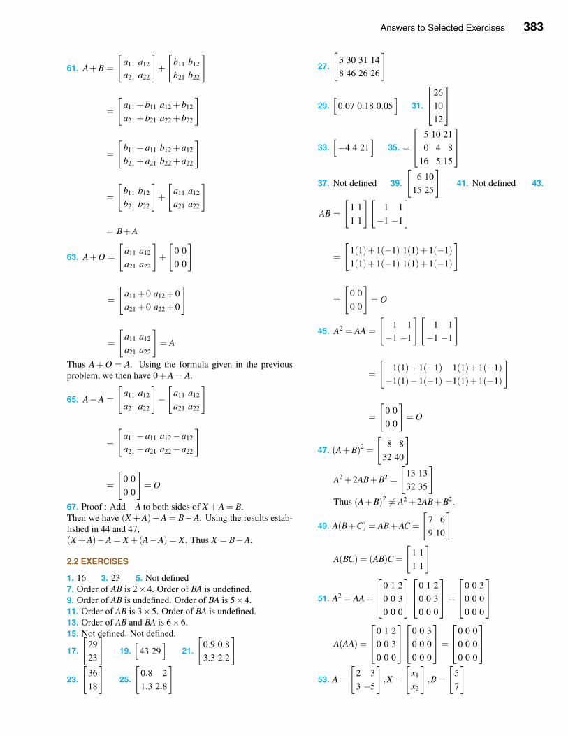
Answers to Selected Exercises 383
61. A+B =
[
a11 a12
a21 a22
]
+
[
b11 b12
b21 b22
]
=
[
a11 +b11 a12 +b12
a21 +b21 a22 +b22
]
=
[
b11 +a11 b12 +a12
b21 +a21 b22 +a22
]
=
[
b11 b12
b21 b22
]
+
[
a11 a12
a21 a22
]
= B+A
63. A+O =
[
a11 a12
a21 a22
]
+
[
0 0
0 0
]
=
[
a11 +0 a12 +0
a21 +0 a22 +0
]
=
[
a11 a12
a21 a22
]
= A
Thus A+O = A. Using the formula given in the previous
problem, we then have 0+A = A.
65. A−A =
[
a11 a12
a21 a22
]
−[
a11 a12
a21 a22
]
=
[
a11−a11 a12−a12
a21−a21 a22−a22
]
=
[
0 0
0 0
]
= O
67. Proof : Add −A to both sides of X +A = B.
Then we have (X +A)−A = B−A. Using the results estab-
lished in 44 and 47,
(X +A)−A = X +(A−A) = X . Thus X = B−A.
2.2 EXERCISES
1. 16 3. 23 5. Not defined
7. Order of AB is 2×4. Order of BA is undefined.
9. Order of AB is undefined. Order of BA is 5×4.
11. Order of AB is 3×5. Order of BA is undefined.
13. Order of AB and BA is 6×6.
15. Not defined. Not defined.
17.
[
29
23
]
19.
[
43 29]
21.
[
0.9 0.8
3.3 2.2
]
23.
[
36
18
]
25.
[
0.8 2
1.3 2.8
]
27.
[
3 30 31 14
8 46 26 26
]
29.
[
0.07 0.18 0.05]
31.
26
10
12
33.
[
−4 4 21]
35. =
5 10 21
0 4 8
16 5 15
37. Not defined 39.
[
6 10
15 25
]
41. Not defined 43.
AB =
[
1 1
1 1
][
1 1
−1 −1
]
=
[
1(1)+1(−1) 1(1)+1(−1)
1(1)+1(−1) 1(1)+1(−1)
]
=
[
0 0
0 0
]
= O
45. A2 = AA =
[
1 1
−1 −1
][
1 1
−1 −1
]
=
[
1(1)+1(−1) 1(1)+1(−1)
−1(1)−1(−1) −1(1)+1(−1)
]
=
[
0 0
0 0
]
= O
47. (A+B)2 =
[
8 8
32 40
]
A2 +2AB+B2 =
[
13 13
32 35
]
Thus (A+B)2 6= A2 +2AB+B2.
49. A(B+C) = AB+AC =
[
7 6
9 10
]
A(BC) = (AB)C =
[
1 1
1 1
]
51. A2 = AA =
0 1 2
0 0 3
0 0 0
0 1 2
0 0 3
0 0 0
=
0 0 3
0 0 0
0 0 0
A(AA) =
0 1 2
0 0 3
0 0 0
0 0 3
0 0 0
0 0 0
=
0 0 0
0 0 0
0 0 0
53. A =
[
2 3
3 −5
]
,X =
[
x1
x2
]
,B =
[
5
7
]
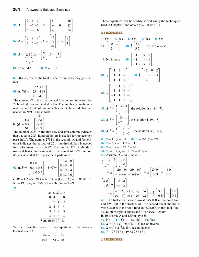
384 Answers to Selected Exercises
55. A =
2 5 3
4 −7 −2
5 −2 6
,X =
x1
x2
x3
,B =
16
12
24
57. A =
[
2 −3 3
5 6 −2
]
,X =
x1
x2
x3
,B =
[
3
1
]
59. A =[
2 3]
,X =
[
x1
x2
]
,B =[
7]
61. H =
3
4.5
4
63. N =
[
3 2 1]
65. MN represents the total of each vitamin the dog gets in a
meal.
67. a. NR =
27 5.3 42
25 4.4 38
21 3.4 35
The number 27 in the first row and first column indicates that
27 hundred tires are needed in LA. The number 38 in the sec-
ond row and third column indicates that 38 hundred plugs are
needed in NYC, and so forth.
b. QC =
$
LA 2954
NYC 2714
SL 2271
The number 2954 in the first row and first column indicates
that a total of 2954 hundred dollars is needed for replacement
parts in LA. The number 2714 in the second row and first col-
umn indicates that a total of 2714 hundred dollars is needed
for replacement parts in NYC. The number 2271 in the third
row and first column indicates that a total of 2271 hundred
dollars is needed for replacement parts in SL.
69. a. B =
0.4 0 0
0.6 1 0.5
0 0 0.5
b. C =
1 0.2 0
0 0.3 0
0 0.2 0.4
0 0.3 0.6
c. W = CZ = C(BY ) = (CB)Y = (CB)(AX) = (CBA)X d.
w1 = 1930, w2 = 1695, w3 = 2266, w4 = 3399
71.
xi yi x2i xiyi
0 4 0 0
1 2 1 2
2 2 4 4
3 1 9 3
4 1 16 4
Sum 10 10 30 13
We then have the system of two equations in the two un-
knowns a and b.
30a + 10b = 13
10a + 5b = 10
These equations can be readily solved using the techniques
used in Chapter 1 and obtain y =−0.7x+3.4.
2.3 EXERCISES
1. Yes 3. Yes 5. Yes 7. Yes 9. Yes
11.
[
10 −3
−3 1
]
13. 17
[
2 1
3 5
]
15. No inverse
17. No inverse 19.
1 −0.5 0
−1 1 −1
1 −0.5 1
21. 13
1 2 4
1 −1 −2
−1 1 −1
23. 1
2
−2 0 2
7 −1 −3
−3 1 1
25. 12
3 −1 −1 −1
1 1 −1 −1
−1 1 1 −1
−1 −1 1 3
27. A−1 =1
2
[
−1 4
−1 2
]
, the solution is (−9,−7).
29. A−1 =
[
3 −1
−2 1
]
, the solution is (9,−3).
31. A−1 =1
2
[
−5 4
3 −2
]
, the solution is (−7,5)
33. x = 11, y =−3 35. x = 11/7, y = 27/7
37. x = 3, y =−1, z =−1
39. x = 2, y =−7/2, z = 3/2
41. x1 =−1, x2 =−1, x3 = 0, x4 = 3
43. Assume D = ad−bc 6= 0.
1D
[
d −b
−c a
][
a b
c d
]
= 1D
[
da−bc db−bd
−ca+ac −cb+ad
]
= 1D
[
D 0
0 D
]
=
[
1 0
0 1
]
[
a b
c d
]
1D
[
d −b
−c a
]
= 1D
[
ad +b(−c) a(−b)+ba
cd +d(−c) c(−b)+da
]
= 1D
[
D 0
0 D
]
=
[
1 0
0 1
]
45. The first client should invest $75,000 in the bond fund
and $25,000 in the stock fund. The second client should in-
vest $25,000 in the bond fund and $25,000 in the stock fund.
47. a. 80 of style A chairs and 40 of style B chairs
b. 10 of style A and 130 of style B
49. No 51. Yes 53. No 55. Yes
57. X = (A+ I)−1B, if (A+ I) has an inverse.
59. X = I +A−1B, if A has an inverse.
61. 74 127 92 54 119 62 27 64 31
2.4 EXERCISES
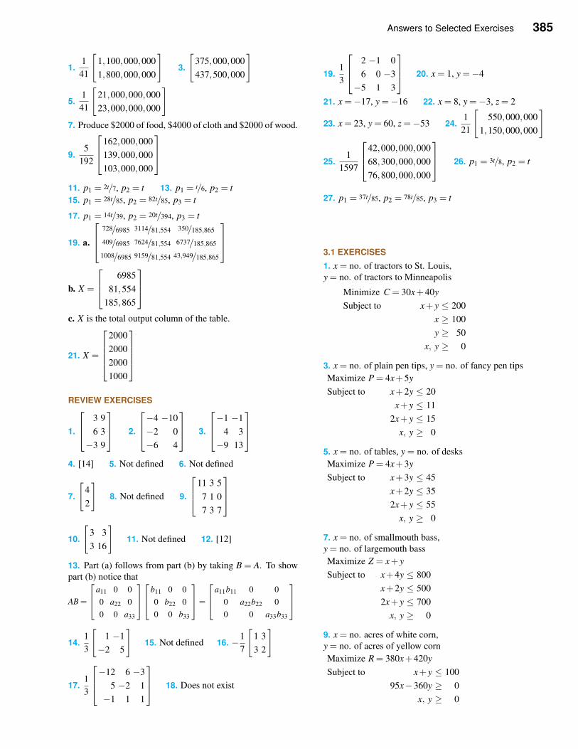
Answers to Selected Exercises 385
1.1
41
[
1,100,000,000
1,800,000,000
]
3.
[
375,000,000
437,500,000
]
5.1
41
[
21,000,000,000
23,000,000,000
]
7. Produce $2000 of food, $4000 of cloth and $2000 of wood.
9.5
192
162,000,000
139,000,000
103,000,000
11. p1 = 2t/7, p2 = t 13. p1 = t/6, p2 = t
15. p1 = 28t/85, p2 = 82t/85, p3 = t
17. p1 = 14t/39, p2 = 20t/394, p3 = t
19. a.
728/6985 3114/81,554 350/185,865
409/6985 7624/81,554 6737/185,865
1008/6985 9159/81,554 43,949/185,865
b. X =
6985
81,554
185,865
c. X is the total output column of the table.
21. X =
2000
2000
2000
1000
REVIEW EXERCISES
1.
3 9
6 3
−3 9
2.
−4 −10
−2 0
−6 4
3.
−1 −1
4 3
−9 13
4. [14] 5. Not defined 6. Not defined
7.
[
4
2
]
8. Not defined 9.
11 3 5
7 1 0
7 3 7
10.
[
3 3
3 16
]
11. Not defined 12. [12]
13. Part (a) follows from part (b) by taking B = A. To show
part (b) notice that
AB =
a11 0 0
0 a22 0
0 0 a33
b11 0 0
0 b22 0
0 0 b33
=
a11b11 0 0
0 a22b22 0
0 0 a33b33
14.1
3
[
1 −1
−2 5
]
15. Not defined 16. −1
7
[
1 3
3 2
]
17.1
3
−12 6 −3
5 −2 1
−1 1 1
18. Does not exist
19.1
3
2 −1 0
6 0 −3
−5 1 3
20. x = 1, y =−4
21. x =−17, y =−16 22. x = 8, y =−3, z = 2
23. x = 23, y = 60, z =−53 24.1
21
[
550,000,000
1,150,000,000
]
25.1
1597
42,000,000,000
68,300,000,000
76,800,000,000
26. p1 = 3t/8, p2 = t
27. p1 = 37t/85, p2 = 78t/85, p3 = t
3.1 EXERCISES
1. x = no. of tractors to St. Louis,
y = no. of tractors to Minneapolis
Minimize C = 30x+40y
Subject to x+ y ≤ 200
x ≥ 100
y ≥ 50
x, y ≥ 0
3. x = no. of plain pen tips, y = no. of fancy pen tips
Maximize P = 4x+5y
Subject to x+2y ≤ 20
x+ y ≤ 11
2x+ y ≤ 15
x, y ≥ 0
5. x = no. of tables, y = no. of desks
Maximize P = 4x+3y
Subject to x+3y ≤ 45
x+2y ≤ 35
2x+ y ≤ 55
x, y ≥ 0
7. x = no. of smallmouth bass,
y = no. of largemouth bass
Maximize Z = x+ y
Subject to x+4y ≤ 800
x+2y ≤ 500
2x+ y ≤ 700
x, y ≥ 0
9. x = no. acres of white corn,
y = no. of acres of yellow corn
Maximize R = 380x+420y
Subject to x+ y ≤ 100
95x−360y ≥ 0
x, y ≥ 0
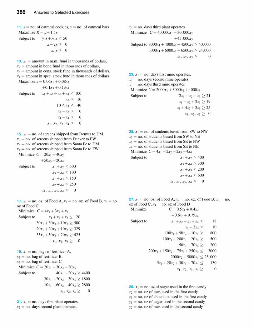
386 Answers to Selected Exercises
11. x = no. of oatmeal cookies, y = no. of oatmeal bars
Maximize R = x+1.5y
Subject to x/18+ y/16 ≤ 50
x−2y ≥ 0
x, y ≥ 0
13. x1 = amount in m.m. fund in thousands of dollars,
x2 = amount in bond fund in thousands of dollars,
x3 = amount in cons. stock fund in thousands of dollars,
x4 = amount in spec. stock fund in thousands of dollars
Maximize z = 0.06x1 +0.08x2
+0.1x3 +0.13x4
Subject to x1 + x2 + x3 + x4 ≤ 100
x3 ≥ 10
10≤ x1 ≤ 40
x2− x3 ≥ 0
x1− x4 ≥ 0
x1, x2, x3, x4 ≥ 0
15. x1 = no. of screens shipped from Denver to DM
x2 = no. of screens shipped from Denver to FW
x3 = no. of screens shipped from Santa Fe to DM
x4 = no. of screens shipped from Santa Fe to FW
Minimize C = 20x1 +40x2
+50x3 +20x4
Subject to x1 + x2 ≤ 500
x3 + x4 ≤ 100
x1 + x3 ≥ 150
x2 + x4 ≥ 250
x1, x2, x3, x4 ≥ 0
17. x1 = no. oz. of Food A, x2 = no. oz. of Food B, x3 = no.
oz of Food C
Minimize C = 4x1 +3x2 + x3
Subject to x1 + x2 + x3 ≤ 20
30x1 +30x2 +10x3 ≥ 500
20x1 +20x2 +10x3 ≥ 329
35x1 +50x2 +20x3 ≥ 425
x1, x2, x3 ≥ 0
19. x1 = no. bags of fertilizer A,
x2 = no. bag of fertilizer B,
x3 = no. bag of fertilizer C
Minimize C = 20x1 +30x2 +20x3
Subject to 40x1 +20x2 ≥ 4400
30x1 +20x2 +30x3 ≥ 1800
10x1 +60x2 +40x3 ≥ 2800
x1, x2, x3 ≥ 0
21. x1 = no. days first plant operates,
x2 = no. days second plant operates,
x3 = no. days third plant operates
Minimize C = 40,000x1 +30,000x2
+45,000x3
Subject to 8000x1 +4000x2 +4500x3 ≥ 40,000
3000x1 +6000x2 +6500x3 ≥ 24,000
x1, x2, x3 ≥ 0
23. x1 = no. days first mine operates,
x2 = no. days second mine operates,
x3 = no. days third mine operates
Minimize C = 2000x1 +3000x2 +4000x3
Subject to 2x1 + x2 + x3 ≥ 21
x1 + x2 +3x3 ≥ 19
x1 +4x2 +3x3 ≥ 25
x1, x2, x3 ≥ 0
25. x1 = no. of students bused from SW to NW
x2 = no. of students bused from SW to NE
x3 = no. of students bused from SE to NW
x4 = no. of students bused from SE to NE
Minimize C = 4x1 +2x2 +2x3 +4x4
Subject to x1 + x2 ≥ 400
x3 + x4 ≥ 300
x1 + x3 ≤ 200
x2 + x4 ≤ 600
x1, x2, x3, x4 ≥ 0
27. x1 = no. oz. of Food A, x2 = no. oz. of Food B, x3 = no.
oz of Food C, x4 = no. oz of Food D
Minimize C = 0.5x1 +0.4x2
+0.6x3 +0.75x4
Subject to x1 + x2 + x3 + x4 ≤ 18
x1 +2x2 ≥ 10
100x1 +50x2 +10x4 ≥ 800
100x1 +200x3 +20x4 ≥ 500
50x3 +70x4 ≥ 200
200x1 +150x2 +75x3 +250x4 ≤ 3000
2000x2 +5000x4 ≤ 25,000
5x1 +20x2 +30x3 +70x4 ≤ 130
x1, x2, x3, x4 ≥ 0
29. x1 = no. oz of sugar used in the first candy
x2 = no. oz of nuts used in the first candy
x3 = no. oz of chocolate used in the first candy
y1 = no. oz of sugar used in the second candy
y2 = no. oz of nuts used in the second candy
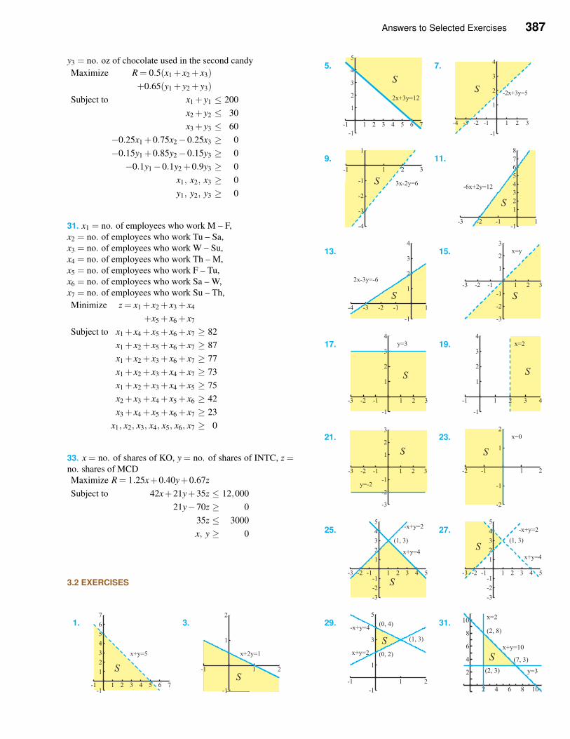
Answers to Selected Exercises 387
y3 = no. oz of chocolate used in the second candy
Maximize R = 0.5(x1 + x2 + x3)
+0.65(y1 + y2 + y3)
Subject to x1 + y1 ≤ 200
x2 + y2 ≤ 30
x3 + y3 ≤ 60
−0.25x1 +0.75x2−0.25x3 ≥ 0
−0.15y1 +0.85y2−0.15y3 ≥ 0
−0.1y1−0.1y2 +0.9y3 ≥ 0
x1, x2, x3 ≥ 0
y1, y2, y3 ≥ 0
31. x1 = no. of employees who work M – F,
x2 = no. of employees who work Tu – Sa,
x3 = no. of employees who work W – Su,
x4 = no. of employees who work Th – M,
x5 = no. of employees who work F – Tu,
x6 = no. of employees who work Sa – W,
x7 = no. of employees who work Su – Th,
Minimize z = x1 + x2 + x3 + x4
+x5 + x6 + x7
Subject to x1 + x4 + x5 + x6 + x7 ≥ 82
x1 + x2 + x5 + x6 + x7 ≥ 87
x1 + x2 + x3 + x6 + x7 ≥ 77
x1 + x2 + x3 + x4 + x7 ≥ 73
x1 + x2 + x3 + x4 + x5 ≥ 75
x2 + x3 + x4 + x5 + x6 ≥ 42
x3 + x4 + x5 + x6 + x7 ≥ 23
x1, x2, x3, x4, x5, x6, x7 ≥ 0
33. x = no. of shares of KO, y = no. of shares of INTC, z =no. shares of MCD
Maximize R = 1.25x+0.40y+0.67z
Subject to 42x+21y+35z ≤ 12,000
21y−70z ≥ 0
35z ≤ 3000
x, y ≥ 0
3.2 EXERCISES
1.
-1 1 2 3 4 5 6 7-1
1
2
3
4
5
6
7
S
x+y=5
3.
-1 1 2
-1
1
2
S
x+2y=1
5.
-1 1 2 3 4 5 6 7-1
1
2
3
4
5
S
2x+3y=12
7.
-4 -3 -2 -1 1 2 3
-1
1
2
3
4
S -2x+3y=5
9.
-1 1 2 3
-4
-3
-2
-1
1
S 3x-2y=6
11.
-3 -2 -1 1-1
12345678
S
-6x+2y=12
13.
-4 -3 -2 -1 1
-1
1
2
3
4
S
2x-3y=-6
15.
-3 -2 -1 1 2 3
-3
-2
-1
1
2
3
S
x=y
17.
-3 -2 -1 1 2 3
-1
1
2
3
4
S
y=3 19.
-1 1 2 3 4
-1
1
2
3
4
S
x=2
21.
-3 -2 -1 1 2 3
-3
-2
-1
1
2
3
S
y=-2
23.
-2 -1 1 2
-2
-1
1
2
S
x=0
25.
-3 -2 -1 1 2 3 4 5
-3
-2
-1
1
2
3
4
5
S
x+y=4
-x+y=2
(1, 3)
27.
-3 -2 -1 1 2 3 4 5
-3
-2
-1
1
2
3
4
5
Sx+y=4
-x+y=2
(1, 3)
29.
-1 1 2-1
1
3
5
Sx+y=2
-x+y=4
(0, 2)
(0, 4)
(1, 3)
31.
2 4 6 8 10
2
4
6
8
10
S
x=2
y=3
x+y=10
(2, 8)
(7, 3)
(2, 3)
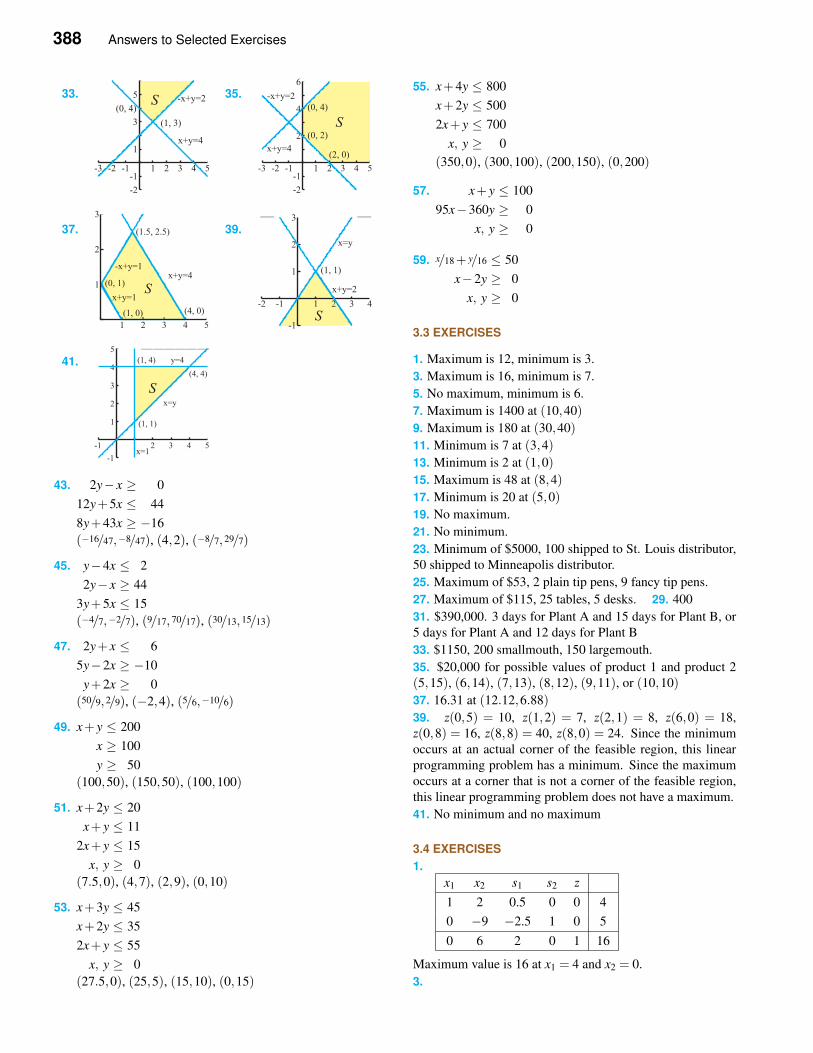
388 Answers to Selected Exercises
33.
-3 -2 -1 1 2 3 4 5
-2
-1
1
3
5S
x+y=4
-x+y=2
(1, 3)
(0, 4)
35.
-3 -2 -1 1 2 3 4 5
-2
-1
2
4
6
S
x+y=4
-x+y=2(0, 4)
(0, 2)
(2, 0)
37.
1 2 3 4 5
1
2
3
S
-x+y=1x+y=4
x+y=1
(4, 0)
(1.5, 2.5)
(1, 0)
(0, 1)
39.
-2 -1 1 2 3 4
-1
1
2
3
S
x=y
x+y=2
(1, 1)
41.
-1 1 2 3 4 5
-1
1
2
3
4
5
Sx=y
x=1
y=4
(4, 4)
(1, 1)
(1, 4)
43. 2y− x ≥ 0
12y+5x ≤ 44
8y+43x ≥ −16
(−16/47,−8/47), (4,2), (−8/7, 29/7)
45. y−4x ≤ 2
2y− x ≥ 44
3y+5x ≤ 15
(−4/7,−2/7), (9/17, 70/17), (30/13, 15/13)
47. 2y+ x ≤ 6
5y−2x ≥ −10
y+2x ≥ 0
(50/9, 2/9), (−2,4), (5/6,−10/6)
49. x+ y ≤ 200
x ≥ 100
y ≥ 50
(100,50), (150,50), (100,100)
51. x+2y ≤ 20
x+ y ≤ 11
2x+ y ≤ 15
x, y ≥ 0
(7.5,0), (4,7), (2,9), (0,10)
53. x+3y ≤ 45
x+2y ≤ 35
2x+ y ≤ 55
x, y ≥ 0
(27.5,0), (25,5), (15,10), (0,15)
55. x+4y ≤ 800
x+2y ≤ 500
2x+ y ≤ 700
x, y ≥ 0
(350,0), (300,100), (200,150), (0,200)
57. x+ y ≤ 100
95x−360y ≥ 0
x, y ≥ 0
59. x/18+ y/16 ≤ 50
x−2y ≥ 0
x, y ≥ 0
3.3 EXERCISES
1. Maximum is 12, minimum is 3.
3. Maximum is 16, minimum is 7.
5. No maximum, minimum is 6.
7. Maximum is 1400 at (10,40)
9. Maximum is 180 at (30,40)
11. Minimum is 7 at (3,4)
13. Minimum is 2 at (1,0)
15. Maximum is 48 at (8,4)
17. Minimum is 20 at (5,0)
19. No maximum.
21. No minimum.
23. Minimum of $5000, 100 shipped to St. Louis distributor,
50 shipped to Minneapolis distributor.
25. Maximum of $53, 2 plain tip pens, 9 fancy tip pens.
27. Maximum of $115, 25 tables, 5 desks. 29. 400
31. $390,000. 3 days for Plant A and 15 days for Plant B, or
5 days for Plant A and 12 days for Plant B
33. $1150, 200 smallmouth, 150 largemouth.
35. $20,000 for possible values of product 1 and product 2
(5,15), (6,14), (7,13), (8,12), (9,11), or (10,10)
37. 16.31 at (12.12,6.88)
39. z(0,5) = 10, z(1,2) = 7, z(2,1) = 8, z(6,0) = 18,
z(0,8) = 16, z(8,8) = 40, z(8,0) = 24. Since the minimum
occurs at an actual corner of the feasible region, this linear
programming problem has a minimum. Since the maximum
occurs at a corner that is not a corner of the feasible region,
this linear programming problem does not have a maximum.
41. No minimum and no maximum
3.4 EXERCISES
1.
x1 x2 s1 s2 z
1 2 0.5 0 0 4
0 −9 −2.5 1 0 5
0 6 2 0 1 16
Maximum value is 16 at x1 = 4 and x2 = 0.
3.
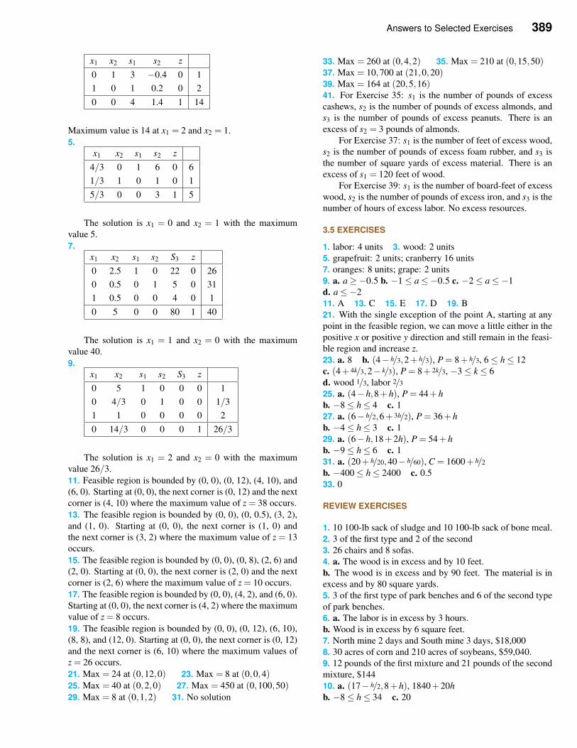
Answers to Selected Exercises 389
x1 x2 s1 s2 z
0 1 3 −0.4 0 1
1 0 1 0.2 0 2
0 0 4 1.4 1 14
Maximum value is 14 at x1 = 2 and x2 = 1.
5.
x1 x2 s1 s2 z
4/3 0 1 6 0 6
1/3 1 0 1 0 1
5/3 0 0 3 1 5
The solution is x1 = 0 and x2 = 1 with the maximum
value 5.
7.
x1 x2 s1 s2 S3 z
0 2.5 1 0 22 0 26
0 0.5 0 1 5 0 31
1 0.5 0 0 4 0 1
0 5 0 0 80 1 40
The solution is x1 = 1 and x2 = 0 with the maximum
value 40.
9.
x1 x2 s1 s2 S3 z
0 5 1 0 0 0 1
0 4/3 0 1 0 0 1/3
1 1 0 0 0 0 2
0 14/3 0 0 0 1 26/3
The solution is x1 = 2 and x2 = 0 with the maximum
value 26/3.
11. Feasible region is bounded by (0, 0), (0, 12), (4, 10), and
(6, 0). Starting at (0, 0), the next corner is (0, 12) and the next
corner is (4, 10) where the maximum value of z = 38 occurs.
13. The feasible region is bounded by (0, 0), (0, 0.5), (3, 2),
and (1, 0). Starting at (0, 0), the next corner is (1, 0) and
the next corner is (3, 2) where the maximum value of z = 13
occurs.
15. The feasible region is bounded by (0, 0), (0, 8), (2, 6) and
(2, 0). Starting at (0, 0), the next corner is (2, 0) and the next
corner is (2, 6) where the maximum value of z = 10 occurs.
17. The feasible region is bounded by (0, 0), (4, 2), and (6, 0).
Starting at (0, 0), the next corner is (4, 2) where the maximum
value of z = 8 occurs.
19. The feasible region is bounded by (0, 0), (0, 12), (6, 10),
(8, 8), and (12, 0). Starting at (0, 0), the next corner is (0, 12)
and the next corner is (6, 10) where the maximum values of
z = 26 occurs.
21. Max = 24 at (0,12,0) 23. Max = 8 at (0,0,4)25. Max = 40 at (0,2,0) 27. Max = 450 at (0,100,50)29. Max = 8 at (0,1,2) 31. No solution
33. Max = 260 at (0,4,2) 35. Max = 210 at (0,15,50)37. Max = 10,700 at (21,0,20)39. Max = 164 at (20,5,16)41. For Exercise 35: s1 is the number of pounds of excess
cashews, s2 is the number of pounds of excess almonds, and
s3 is the number of pounds of excess peanuts. There is an
excess of s2 = 3 pounds of almonds.
For Exercise 37: s1 is the number of feet of excess wood,
s2 is the number of pounds of excess foam rubber, and s3 is
the number of square yards of excess material. There is an
excess of s1 = 120 feet of wood.
For Exercise 39: s1 is the number of board-feet of excess
wood, s2 is the number of pounds of excess iron, and s3 is the
number of hours of excess labor. No excess resources.
3.5 EXERCISES
1. labor: 4 units 3. wood: 2 units
5. grapefruit: 2 units; cranberry 16 units
7. oranges: 8 units; grape: 2 units
9. a. a≥−0.5 b. −1≤ a≤−0.5 c. −2≤ a≤−1
d. a≤−2
11. A 13. C 15. E 17. D 19. B
21. With the single exception of the point A, starting at any
point in the feasible region, we can move a little either in the
positive x or positive y direction and still remain in the feasi-
ble region and increase z.
23. a. 8 b. (4− h/3,2+ h/3), P = 8+ h/3, 6≤ h≤ 12
c. (4+ 4k/3,2− k/3), P = 8+ 2k/3, −3≤ k ≤ 6
d. wood 1/3, labor 2/3
25. a. (4−h,8+h), P = 44+h
b. −8≤ h≤ 4 c. 1
27. a. (6− h/2,6+ 3h/2), P = 36+h
b. −4≤ h≤ 3 c. 1
29. a. (6−h,18+2h), P = 54+h
b. −9≤ h≤ 6 c. 1
31. a. (20+ h/20,40− h/60), C = 1600+ h/2
b. −400≤ h≤ 2400 c. 0.5
33. 0
REVIEW EXERCISES
1. 10 100-lb sack of sludge and 10 100-lb sack of bone meal.
2. 3 of the first type and 2 of the second
3. 26 chairs and 8 sofas.
4. a. The wood is in excess and by 10 feet.
b. The wood is in excess and by 90 feet. The material is in
excess and by 80 square yards.
5. 3 of the first type of park benches and 6 of the second type
of park benches.
6. a. The labor is in excess by 3 hours.
b. Wood is in excess by 6 square feet.
7. North mine 2 days and South mine 3 days, $18,000
8. 30 acres of corn and 210 acres of soybeans, $59,040.
9. 12 pounds of the first mixture and 21 pounds of the second
mixture, $144
10. a. (17− h/2,8+h), 1840+20h
b. −8≤ h≤ 34 c. 20
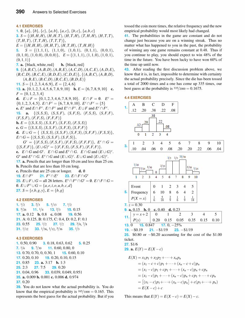
390 Answers to Selected Exercises
4.1 EXERCISES
1. /0, {a}, {b}, {c}, {a,b}, {a,c}, {b,c}, {a,b,c}3. S = {(H,H,H), (H,H,T ), (H,T,H), (T,H,H), (H,T,T ),(T,H,T ), (T,T,H), (T,T,T )},E = {(H,H,H), (H,H,T ), (H,T,H), (T,H,H)}5. S = {(1,1,1), (1,1,0), (1,0,1), (0,1,1), (0,0,1),(0,1,0), (1,0,0), (0,0,0)}, E = {(1,1,1), (1,1,0), (1,0,1),(0,1,1)}7. a. {black,white, red} b. {black, red}9. {(A,B,C),(A,B,D),(A,B,E),(A,C,D),(A,C,E),(A,D,E),(B,C,D),(B,C,E),(B,D,E),(C,D,E)}, {(A,B,C),(A,B,D),
(A,B,E),(B,C,D),(B,C,E),(B,D,E)}11. S = {1,2,3,4,6,9}, E = {2,4,6}13. a. {0,1,2,3,4,5,6,7,8,9,10} b. E = {6,7,8,9,10} c.
F = {0,1,2,3,4}d. E ∪ F = {0,1,2,3,4,6,7,8,9,10}. E ∩ F = /0. Ec ={0,1,2,3,4,5}. E ∩Fc = {6,7,8,9,10}. Ec∩Fc = {5}e. Ec and E ∩Fc. E ∩Fc and Ec∩Fc. E ∪F and Ec∩Fc.
15. a. {(S,S,S), (S,S,F), (S,F,S), (F,S,S), (S,F,F),(F,S,F), (F,F,S), (F,F,F)}b. E = {(S,S,S),(S,S,F),(S,F,S),(F,S,S)}c. G = {(S,S,S),(S,S,F),(S,F,S),(S,F,F)}d. E ∪G = { (S,S,S),(S,S,F),(S,F,S),(S,F,F),(F,S,S)},E ∩G = {(S,S,S),(S,S,F),(S,F,S)},
Gc = {(F,S,S),(F,S,F),(F,F,S),(F,F,F)}, Ec ∩ G ={(S,F,F)}, (E ∪G)c = {(F,F,S),(F,S,F),(F,F,F)}.e. E ∩G and Gc. E ∩G and Ec ∩G. E ∩G and (E ∪G)c.
Gc and Ec∩G. Ec∩G and (E ∪G)c. E ∪G and (E ∪G)c.
17. a. Pencils that are longer than 10 cm and less than 25 cm.
b. Pencils that are less than 10 cm long.
c. Pencils that are 25 cm or longer. d. /0
19. E ∩Fc 21. Fc∩Ec 23. E ∩F ∩Gc
25. E∪F ∪G = all 26 letters. Ec∩Fc∩Gc = /0. E∩F ∩G =/0. E ∪Fc∪G = {a,e, i,o,u,b,c,d}27. S = {r,b,g,y}, E = {b,g}
4.2 EXERCISES
1. 1/2 3. 2/3 5. 1/13 7. 1/2
9. 3/26 11. 1/4 13. 2/3 15. 0.15
17. a. 0.12 b. 0.8 c. 0.08 19. 0.56
21. A: 0.125, B: 0.175, C: 0.4, D: 0.2, F: 0.1
23. 0.55 25. 1/2 27. 1/2 29. 3/8, 7/8
31. 1/12 33. 1/36, 1/12, 5/36 35. 1/3
4.3 EXERCISES
1. 0.50, 0.90 3. 0.18, 0.63, 0.62 5. 0.25
7. 1/6 9. 7/30 11. 0.60, 0.80, 0
13. 0.70, 0.70, 0, 0.30, 1 15. 0.60, 0.10
17. 0.20, 0.10 19. 0.20, 0.10, 0.15
21. 0.85 23. a. 3:17 b. 1:3
25. 2:3 27. 7:5 29. 0.20
31. 0.04, 0.96 33. 0.039, 0.049, 0.951
35. a. 0.009 b. 0.001 c. 0.006 d. 0.974
37. 0.20
39. You do not know what the actual probability is. You do
know that the empirical probability is 165/1000 = 0.165. This
represents the best guess for the actual probability. But if you
tossed the coin more times, the relative frequency and the new
empirical probability would most likely had changed.
41. The probabilities in the game are constant and do not
change just because you are on a winning streak. Thus no
matter what has happened to you in the past, the probability
of winning any one game remains constant at 0.48. Thus if
you continue to play, you should expect to win 48% of the
time in the future. You have been lucky to have won 60% of
the time up until now.
43. After reading the first discussion problem above, we
know that it is, in fact, impossible to determine with certainty
the actual probability precisely. Since the die has been tossed
a total of 2000 times and a one has come up 335 times, our
best guess at the probability is 335/2000 = 0.1675.
4.4 EXERCISES
1.A B C D F
.12 .20 .38 .22 .08
3.1 2 3 4 5 6 7 8 9 10
.10 .04 .06 0 .08 .20 .20 .22 .06 .04
5.
Event 0 1 2 3 4 5
Frequency 6 10 8 6 4 2
P(X = x) 16
518
29
16
19
118
7. z = 0.30
9. a. 0.15 b. 0 c. 0.40 d. 0.23
11.y = x+2 0 1 2 3 4 5
P(y) 0.20 0.15 0.05 0.35 0.15 0.10
13. 0 15. 0.847 17. 0, −25%
19. −$0.19 21. −$1/19 23. −$1/19
25. $0.80 or −$0.20 accounting for the cost of the $1.00
ticket.
27. $1/6
29. a. E(Y ) = E(X− c)
E(X) = x1 p1 + x2 p2 + · · ·+ xn pn
= (x1− c+ c)p1 + · · ·+(xn− c+ c)pn
= (x1− c)p1 + cp1 + · · ·+(xn− c)pn + cpn
= (x1− c)p1 + · · ·+(xn− c)pn + cp1 + · · ·+ cpn
=[(x1− c)p1+· · ·+(xn− c)pn
]+ c(p1+· · ·+ pn)
= E(X− c)+ c
This means that E(Y ) = E(X− c) = E(X)− c.
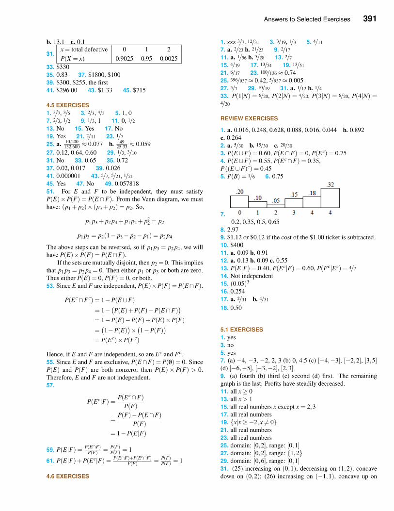
Answers to Selected Exercises 391
b. 13.1 c. 0.1
31.x = total defective 0 1 2
P(X = x) 0.9025 0.95 0.0025
33. $330
35. 0.83 37. $1800, $100
39. $300, $255, the first
41. $296.00 43. $1.33 45. $715
4.5 EXERCISES
1. 3/7, 3/5 3. 2/3, 4/5 5. 1, 0
7. 2/3, 1/2 9. 1/3, 1 11. 0, 1/2
13. No 15. Yes 17. No
19. Yes 21. 2/11 23. 1/7
25. a. 10,200132,600 ≈ 0.077 b. 49
25·33 ≈ 0.059
27. 0.12, 0.64, 0.60 29. 1/3, 3/10
31. No 33. 0.65 35. 0.72
37. 0.02, 0.017 39. 0.026
41. 0.000001 43. 5/7, 5/21, 1/21
45. Yes 47. No 49. 0.057818
51. For E and F to be independent, they must satisfy
P(E)×P(F) = P(E ∩F). From the Venn diagram, we must
have: (p1 + p2)× (p3 + p2) = p2. So,
p1 p3 + p2 p3 + p1 p2 + p22 = p2
p1 p3 = p2(1− p3− p2− p1) = p2 p4
The above steps can be reversed, so if p1 p3 = p2 p4, we will
have P(E)×P(F) = P(E ∩F).If the sets are mutually disjoint, then p2 = 0. This implies
that p1 p3 = p2 p4 = 0. Then either p1 or p3 or both are zero.
Thus either P(E) = 0, P(F) = 0, or both.
53. Since E and F are independent, P(E)×P(F) = P(E∩F).
P(Ec∩Fc) = 1−P(E ∪F)
= 1−(P(E)+P(F)−P(E ∩F)
)
= 1−P(E)−P(F)+P(E)×P(F)
=(1−P(E)
)×(1−P(F)
)
= P(Ec)×P(Fc)
Hence, if E and F are independent, so are Ec and Fc.
55. Since E and F are exclusive, P(E∩F) = P( /0) = 0. Since
P(E) and P(F) are both nonzero, then P(E)× P(F) > 0.
Therefore, E and F are not independent.
57.
P(Ec|F) =P(Ec∩F)
P(F)
=P(F)−P(E ∩F)
P(F)
= 1−P(E|F)
59. P(E|F) = P(E∩F)P(F) = P(F)
P(F) = 1
61. P(E|F)+P(Ec|F) = P(E∩F)+P(Ec∩F)P(F) = P(F)
P(F) = 1
4.6 EXERCISES
1. zzz 3/7, 12/31 3. 3/19, 1/3 5. 4/11
7. a. 2/23 b. 21/23 9. 2/17
11. a. 1/56 b. 5/28 13. 2/7
15. 4/19 17. 13/51 19. 13/51
21. 6/17 23. 100/136≈ 0.74
25. 396/937≈ 0.42, 5/937≈ 0.005
27. 5/7 29. 10/19 31. a. 1/12 b. 1/4
33. P(1|N) = 6/20, P(2|N) = 4/20, P(3|N) = 6/20, P(4|N) =4/20
REVIEW EXERCISES
1. a. 0.016, 0.248, 0.628, 0.088, 0.016, 0.044 b. 0.892
c. 0.264
2. a. 5/30 b. 15/30 c. 20/30
3. P(E ∪F) = 0.60, P(E ∩F) = 0, P(Ec) = 0.75
4. P(E ∪F) = 0.55, P(Ec∩F) = 0.35,
P((E ∪F)c) = 0.45
5. P(B) = 1/6 6. 0.75
7.
0.2, 0.35, 0.5, 0.65
8. 2.97
9. $1.12 or $0.12 if the cost of the $1.00 ticket is subtracted.
10. $400
11. a. 0.09 b. 0.91
12. a. 0.13 b. 0.09 c. 0.55
13. P(E|F) = 0.40, P(Ec|F) = 0.60, P(Fc|Ec) = 4/7
14. Not independent
15. (0.05)3
16. 0.254
17. a. 2/31 b. 4/31
18. 0.50
5.1 EXERCISES
1. yes
3. no
5. yes
7. (a) −4, −3, −2, 2, 3 (b) 0, 4.5 (c) [−4,−3], [−2,2], [3,5](d) [−6,−5], [−3,−2], [2,3]9. (a) fourth (b) third (c) second (d) first. The remaining
graph is the last: Profits have steadily decreased.
11. all x≥ 0
13. all x > 1
15. all real numbers x except x = 2,317. all real numbers
19. {x|x≥−2,x 6= 0}21. all real numbers
23. all real numbers
25. domain: [0,2], range: [0,1]27. domain: [0,2], range: {1,2}29. domain: [0,6], range: [0,1]31. (25) increasing on (0,1), decreasing on (1,2), concave
down on (0,2); (26) increasing on (−1,1), concave up on
392 Answers to Selected Exercises
(−1,0), concave down on (0,1); (28) increasing on (−1,1)and (1,2), concave up on (1,2), concave down on (−1,1)
33.1
2,
2
3, −1,
1√2
,1
x+3,
x+1
x+2
35. 3, 0,√
2x2−2,√
2/x−1,√−2x−1, −
√2x−1,
37. 1, −1, |x|, x2
39. 1, 2, 2, 2
41. 0, 1, 0, 1
43. yes
45. no
47. no
49. yes
51. Continuous everywhere except x =−1.
53. Continuous everywhere.
55. Continuous everywhere except x = 1.
57. Continuous everywhere except at x = 1 and x = 2.
59. all real numbers
61. [−3,3]63. [0,5)∪ (5,∞)65. 0, 2, 3, 4
67. V (x) = 3x3
69. d(t) = 60t
71. R(x) = 60x
73.
C(x) =
{
x if 0≤ x≤ 500
500+2(x−500) if x > 500
This function is continuous on [0,∞).75.
T (x) =
{
0 if 0≤ x≤ 50
0.01(x−50) if x > 50
Continuous on [0,∞).77.
P(x) =
0.37 if 0≤ x≤ 1
0.60 if 1 < x≤ 2
0.83 if 2 < x≤ 3
Continuous on [0,3] except at x = 1 and x = 2.
79. A(10) = 0.80. There are 0.80 fish on average in a cu-
bic meters of water that’s at 100C. A(13) = 1.15. There are
1.15 fish on average in a cubic meters of water that’s at 130C.
A(19) = 0. There are no fish on average in a cubic meters of
water that’s at 190C.
There are no fish if the water temperature is too cold or
too warm. As the temperature increases, so do the number of
fish. However, at some point, the number decreases.
81. N(0) = 0. There are no fish at the surface. N(120) = 20.
Twenty fish were caught at a depth of 120 meters. N(300)≈0. There are no fish at a depth of 300 meters.
83. 109.6, 70.5
85.
T (x)=
0.15x if x≤ 27,050
4057.50+0.275(x−27,050) if 27,050 < x≤ 65,550
14,645+0.305(x−65,550) if 65,550 < x≤ 136,750
36,361+0.355(x−136,750) if 136,750 < x≤ 297,350
93,374+0.391(x−297,350) if x > 297,350
87. S(118) ≈ 7. This means that in 118 square meters of
woodland, there are about 7 species of plants. S(0.5A) =(0.5)0.284S(A) ≈ 0.82S(A), so when the area is reduced by
one half, the number of species is reduced by a factor of about
0.82.
89. 3
91. 6x+3h
93.
f (x) =
{
3x−2 if x≥ 2
x+2 if x < 2
95. The two functions are the same.
97. f (a+b) = m(a+b) = ma+mb = f (a)+ f (b)99. 3 f (x) = 3 · 3x = 3x+1 = f (x + 1), f (a + b) = 3a+b =3a ·3b = f (a) · f (b)
5.2 EXERCISES
1. C = 3x+10,000
3. R = 5x
5. P = 2x−10,000
7. x = 2
9. x = 20
11. (1.5,4.5)13. (1,15)15. x = 5
17. x = 1.519. P(x) = −2x2 + 20x− 42, maximum when x = 5, break-
even quantities are x = 3,721. P(x) =−x2+15x−36, maximum when x = 15/2, break-
even quantities are x = 3,12
23. Break-even quantities are x = 0.9 and 2.2. Maximum at
x = 1.55.
25. Break-even quantities are approximately x = 2.11, 7.23.
Maximum at x = 4.67.
27. V =−5000t +50,000, $45,000, $25,000
29. p =−0.005x+22.531. Let x be the number of pairs of fenders manufactured.
Then the costs functions in dollars are as follows:
Steel: C(x) = 260,000+5.26x
Aluminum: C(x) = 385,000+12.67x
RMP: C(x) = 95,000+13.19x
NPN: C(x) = 95,000+9.53x
PPT: C(x) = 95,000+12.55x
33. 12,000
35. Let x be the number of cows, then the cost C(x) in
dollors is C(x) = 13,386 + 393x. The revenue function in
dollars is R(x) = 470x. The profit function in dollars is
P(x) = 77x− 13,386. The profit for an average of 97 cows
is P(97) = −5917, that is a loss of $5917. For many such
farms the the property and buildings have already been paid
off. Thus, the fixed costs for these farms are lower than stated
in the table.
37. C = 209.03x + 447,917, R = 266.67x, P = 57.64x−447,917
39. outside
41. (a) f = 0.3056x; (b) c = 3525+0.3056x; (c) $4289
Answers to Selected Exercises 393
43. Let x be the number of copies. The cost in cents with
no plastic card is C(x) = 10x. The cost with a plastic card is
C(x) = 50+7x. 17.
45. Decreases by 0.108475 yen per ton. This number s the
slope of the line.
47. 110
49. 5593 bales, 30,000 bales
51. 63.8, 2.95116
53. 3 pounds, the relative yield of vegetables is maximized
55. 11666.67, 58.46
57. 35
59. (a) 30.74; (b) 19.91; (c) 41.57
61. C = 5x+1000
63. C = 3x+2000
65. R = 11x
67. (a) manual; (b) automatic
Total Costs
Volume Manual Automatic
1000 $2600 $8020
10,000 $17,000 $8200
69.
Costs Per Unit
Volume Manual Automatic
1000 $2.60 $8.02
10,000 $1.70 $0.82
100,000 $1.61 $0.10
Cm =1000
x+ 1.6, Ca =
8000
x+ 0.02. The cost per
unit for a manual machine tends toward $1.60 and becomes
greater than the cost per unit for an automatic machine, which
tends toward $0.02.
71. α = 2, β = 8
73. Since we expect profits to turn negative if too many prod-
ucts are made and sold (the price would have to be very low
to unload so many products), a should be negative.
75. The graph of p = mx + e should slope downward, re-
quiring m < 0 and e > 0. Since R = xp = mx2 + ex and
R = ax2 +bx, a = m < 0 and b = e > 0.
77. approximately 2%, 4%
79. The fewer the number of boat trips, the more the owner
needs to charge to make a living. But, at some point, the price
is so high that nobody will be willing to pay such a high price.
The industry refers to this as the “choke” price.
81. about 20. There are about 0.72 times the original, or a
28% drop
83. about 7. about 66%
5.3 EXERCISES
1.
3.
5.
7.
9. 2
11.3
4
13.3
4
15. −45
2317.
19.
21.
23.
25. −1
27. −3
29. −1
2
31. −1
233. 1
35. −1
37. 0, 1
39. (a) $1080; (b) $1082.43; (c) $1083.00; (d) $1083.22; (e)
$1083.28; (f) $1083.29
41. (a) $3262.04; (b) $7039.99; (c) $14,974.46; (d)
$31,409.42; (e) $93,050.97; (f) $267,863.55
43. (a) 8.16%; (b) 8.243%; (c) 8.300%; (d) 8.322%; (e)
8.328% (f) 8.329%
45. (a) $1784.31; (b) $1664.13; (c) $1655.56; (d) $1652.99
47. $31,837.58
49. $26,897.08
51. $5.5 trillion
53. $2602, yes
55. 6.66%, 6.82%, the second bank
57. $67,297.13
59. 11.58 years
61. 8.2%
63. The second bank, the second effective interest rate is
greater than the first one.
65. about 3.7 years
67. $568.95
69. 6.8 billion
71. 5%
73. 16.82
75. (0,∞), (−∞,0)77. P = 32(0.5)x
79. increasing. 346 mm. 736 grams.
81. About 20 feet.
5.4 EXERCISES
1. (a) 11; (b) 3; (c) 28; (d) 7/4
3. x2 + 2x+ 4, −x2 + 2x+ 2, (2x+ 3)(x2 + 1),2x+3
x2 +1. All
domains are (−∞,∞).
5. 3x+4, x+2, 2x2 +5x+3,2x+3
x+1. The domain is (−∞,∞)
in the first three cases and (−∞,−1)∪(−1,∞) in the last case.
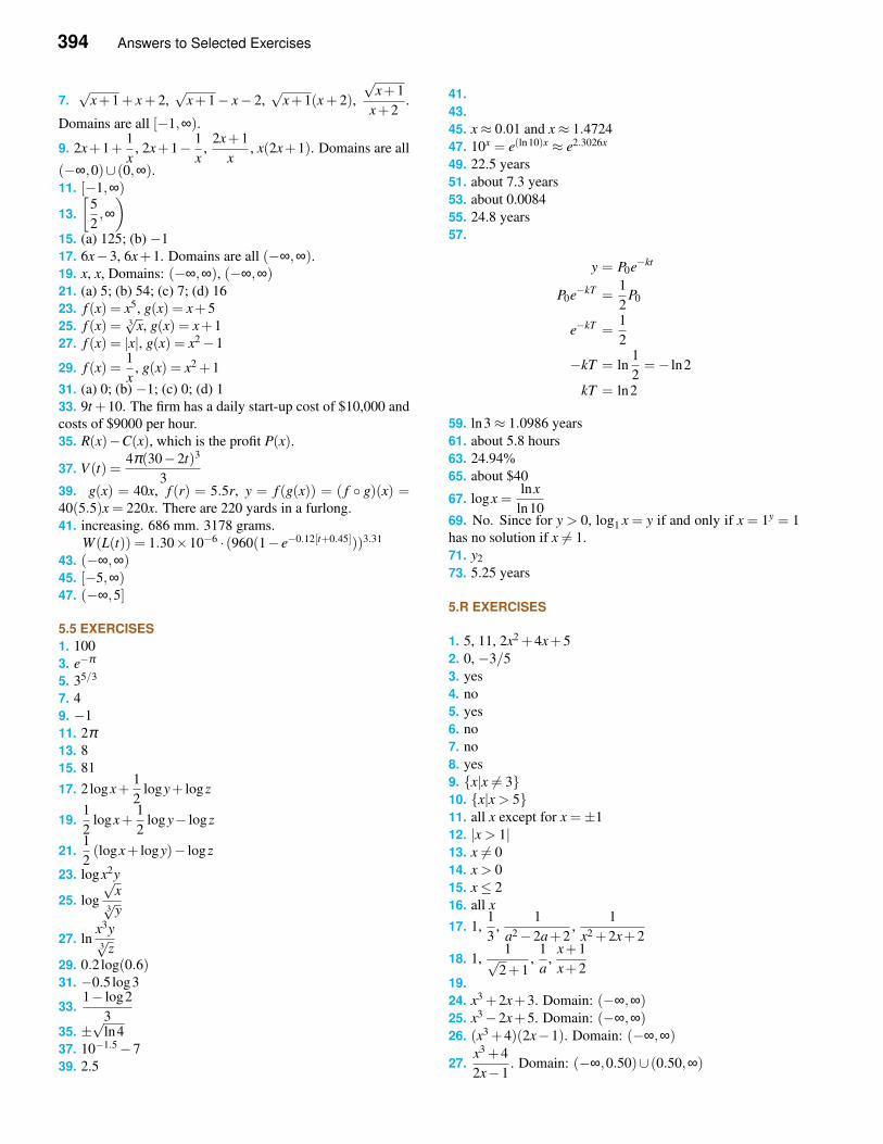
394 Answers to Selected Exercises
7.√
x+1+ x+ 2,√
x+1− x− 2,√
x+1(x+ 2),
√x+1
x+2.
Domains are all [−1,∞).
9. 2x+1+1
x, 2x+1− 1
x,
2x+1
x, x(2x+1). Domains are all
(−∞,0)∪ (0,∞).11. [−1,∞)
13.
[5
2,∞)
15. (a) 125; (b) −1
17. 6x−3, 6x+1. Domains are all (−∞,∞).19. x, x, Domains: (−∞,∞), (−∞,∞)21. (a) 5; (b) 54; (c) 7; (d) 16
23. f (x) = x5, g(x) = x+5
25. f (x) = 3√
x, g(x) = x+1
27. f (x) = |x|, g(x) = x2−1
29. f (x) =1
x, g(x) = x2 +1
31. (a) 0; (b) −1; (c) 0; (d) 1
33. 9t +10. The firm has a daily start-up cost of $10,000 and
costs of $9000 per hour.
35. R(x)−C(x), which is the profit P(x).
37. V (t) =4π(30−2t)3
339. g(x) = 40x, f (r) = 5.5r, y = f (g(x)) = ( f ◦ g)(x) =40(5.5)x = 220x. There are 220 yards in a furlong.
41. increasing. 686 mm. 3178 grams.
W (L(t)) = 1.30×10−6 · (960(1− e−0.12[t+0.45]))3.31
43. (−∞,∞)45. [−5,∞)47. (−∞,5]
5.5 EXERCISES
1. 100
3. e−π
5. 35/3
7. 4
9. −1
11. 2π13. 8
15. 81
17. 2logx+1
2logy+ logz
19.1
2logx+
1
2logy− logz
21.1
2(logx+ logy)− logz
23. logx2y
25. log
√x
3√
y
27. lnx3y
3√
z
29. 0.2log(0.6)31. −0.5log3
33.1− log2
335. ±
√ln4
37. 10−1.5−7
39. 2.5
41.
43.
45. x≈ 0.01 and x≈ 1.4724
47. 10x = e(ln10)x ≈ e2.3026x
49. 22.5 years
51. about 7.3 years
53. about 0.0084
55. 24.8 years
57.
y = P0e−kt
P0e−kT =1
2P0
e−kT =1
2
−kT = ln1
2=− ln2
kT = ln2
59. ln3≈ 1.0986 years
61. about 5.8 hours
63. 24.94%
65. about $40
67. logx =lnx
ln1069. No. Since for y > 0, log1 x = y if and only if x = 1y = 1
has no solution if x 6= 1.
71. y2
73. 5.25 years
5.R EXERCISES
1. 5, 11, 2x2 +4x+5
2. 0, −3/5
3. yes
4. no
5. yes
6. no
7. no
8. yes
9. {x|x 6= 3}10. {x|x > 5}11. all x except for x =±1
12. |x > 1|13. x 6= 0
14. x > 0
15. x≤ 2
16. all x
17. 1,1
3,
1
a2−2a+2,
1
x2 +2x+2
18. 1,1√
2+1,
1
a,
x+1
x+219.
24. x3 +2x+3. Domain: (−∞,∞)25. x3−2x+5. Domain: (−∞,∞)26. (x3 +4)(2x−1). Domain: (−∞,∞)
27.x3 +4
2x−1. Domain: (−∞,0.50)∪ (0.50,∞)
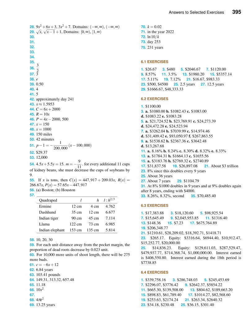
Answers to Selected Exercises 395
28. 9x2 +6x+3, 3x2 +7. Domains: (−∞,∞), (−∞,∞)29.√
x,√
x−1+1, Domains: [0,∞), [1,∞)30.
31.
32.
33.
34.
35.
36.3
237. 3
38. e
39. 0.50
40. 4
41. 5
42. approximately day 241
43. x≈ 1.5953
44. C = 6x+2000
45. R = 10x
46. P = 4x−2000, 500
47. x = 150
48. x = 1000
49. 150 miles
50. 42 minutes
51. p−1 =− 1
200,000(x−100,000)
52. $29.37
53. 12,000
54. 4.5x+5.5y = 15. m =− 9
11. for every additional 11 cups
of kidney beans, she must decrease the cups of soybeans by
9.
55. If x is tons, then C(x) = 447,917 + 209.03x, R(x) =266.67x, P(x) = 57.65x−447,917
56. (a) Boston; (b) Houston
57.
Quadraped l h l : h2/3
Ermine 12 cm 4 cm 4.762
Dashhund 35 cm 12 cm 6.677
Indian tiger 90 cm 45 cm 7.114
Llama 122 cm 73 cm 6.985
Indian elephant 153 cm 135 cm 5.814
58. 10, 20, 30
59. For each unit distance away from the pocket margin, the
proportion of dead roots decrease by 0.023 unit.
60. For 10,000 more units of shoot length, there will be 275
more buds.
61. c =−6x+12
62. 6.84 years
63. 103.41 pounds
64. 149.31, 313.32, 657.48
65. 11.18
66. 10x2
67.
68. 4πt2
69. 13.25 years
70. k = 0.02
71. in the year 2022
72. ln10/k
73. day 253
75. 231 years
6.1 EXERCISES
1. $26.67 3. $480 5. $2046.67 7. $1120.00
9. 8.57% 11. 3.5% 13. $1980.20 15. $5357.14
17. 5.11% 19. 7.12% 21. $16.67, $983.33
23. $500, $4500 25. 2.5 years 27. 12.5 years
29. $1666.67, $48,333.33
6.2 EXERCISES
1. $1100.00
3. a. $1080.00 b. $1082.43 c. $1083.00
d. $1083.22 e. $1083.28
5. a. $21,724.52 b. $23,769.91 c. $24,273.39
d. $24,472.28 e. $24,523.94
7. a. $3262.04 b. $7039.99 c. $14,974.46
d. $31,409.42 e. $93,050.97 f. $267,863.55
9. a. $1538.62 b. $2367.36 c. $3642.48
d. $13,267.68
11. a. 8.16% b. 8.24% c. 8.30% d. 8.32% e. 8.33%
13. a. $1784.31 b. $1664.13 c. $1655.56
15. a. $3183.76 b. $2769.32 c. $2740.89
17. $31,837.58 19. $26,897.08 21. About $3 trillion
23. 8% since this doubles every 9 years
25. About 36 years
27. About 7 years 29. $1104.79
31. At 8% $1000 doubles in 9 years and at 9% doubles again
after 8 years, ending with $4000.
33. 8.26%, 8.32%, second 35. $70,485.40
6.3 EXERCISES
1. $17,383.88 3. $18,120.60 5. $98,925.54
7. $15,645.49 9. $2,045,953.85 11. $1316.40
13. $148.36 15. $7.23 17. $675,764.89
19. $206,348.77
21. $1210.61, $28,209.02, $18,392.71, $1418.71
23. $265.17. Equity: $3316.64, $6944.40, $10,912.47,
$15,252.77, $20,000.00
25. $14,836.23. Equity: $129,611.03, $287,529.47,
$479,937.77, $714,368.74, $1,000,000.00. Interest earned
is $406,550.80. Interest earned during the 18th period is
$7738.85
6.4 EXERCISES
1. $339,758.16 3. $286,748.03 5. $245,453.69
7. $2296.07, $3776.42 9. $2642.37, $5854.22
11. $665.30, $139,508.00 13. $804.62, $189,663.20
15. $898.83, $61,789.40 17. $1014.27, $82,568.60
19. $253.63, $2174.24 21. $263.34, $2640.32
23. $34.18, $230.48 25. $36.15, $301.40
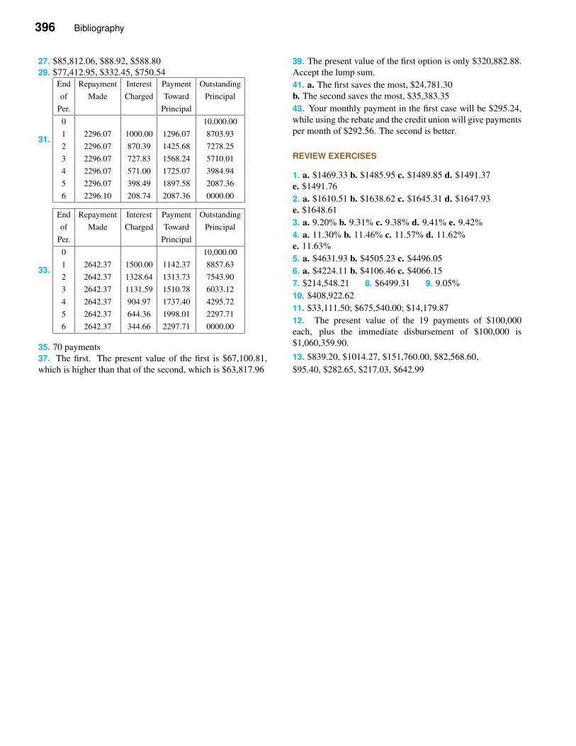
396 Bibliography
27. $85,812.06, $88.92, $588.80
29. $77,412.95, $332.45, $750.54
31.
End Repayment Interest Payment Outstanding
of Made Charged Toward Principal
Per. Principal
0 10,000.00
1 2296.07 1000.00 1296.07 8703.93
2 2296.07 870.39 1425.68 7278.25
3 2296.07 727.83 1568.24 5710.01
4 2296.07 571.00 1725.07 3984.94
5 2296.07 398.49 1897.58 2087.36
6 2296.10 208.74 2087.36 0000.00
33.
End Repayment Interest Payment Outstanding
of Made Charged Toward Principal
Per. Principal
0 10,000.00
1 2642.37 1500.00 1142.37 8857.63
2 2642.37 1328.64 1313.73 7543.90
3 2642.37 1131.59 1510.78 6033.12
4 2642.37 904.97 1737.40 4295.72
5 2642.37 644.36 1998.01 2297.71
6 2642.37 344.66 2297.71 0000.00
35. 70 payments
37. The first. The present value of the first is $67,100.81,
which is higher than that of the second, which is $63,817.96
39. The present value of the first option is only $320,882.88.
Accept the lump sum.
41. a. The first saves the most, $24,781.30
b. The second saves the most, $35,383.35
43. Your monthly payment in the first case will be $295.24,
while using the rebate and the credit union will give payments
per month of $292.56. The second is better.
REVIEW EXERCISES
1. a. $1469.33 b. $1485.95 c. $1489.85 d. $1491.37
e. $1491.76
2. a. $1610.51 b. $1638.62 c. $1645.31 d. $1647.93
e. $1648.61
3. a. 9.20% b. 9.31% c. 9.38% d. 9.41% e. 9.42%
4. a. 11.30% b. 11.46% c. 11.57% d. 11.62%
e. 11.63%
5. a. $4631.93 b. $4505.23 c. $4496.05
6. a. $4224.11 b. $4106.46 c. $4066.15
7. $214,548.21 8. $6499.31 9. 9.05%
10. $408,922.62
11. $33,111.50; $675,540.00; $14,179.87
12. The present value of the 19 payments of $100,000
each, plus the immediate disbursement of $100,000 is
$1,060,359.90.
13. $839.20, $1014.27, $151,760.00, $82,568.60,
$95.40, $282.65, $217.03, $642.99
Bibliography
Aadland, D. and A. J. Caplan (2003). Willingness to pay for curbside recycling
with detection and mitigation of hypothetical bias. Amer. J. Agr. Econ. 85(2),
492–502.
Antle, J. M. and S. M. Capalbo (2001). Econometric-process models for
integrated assessment of agricultural production systems. Amer. J. Agr.
Econ. 83(2), 389–401.
Bell, F. W. (1986). Competition from fish farming in influencing rent dissipation:
The crayfish fishery. Amer. J. Agr. Econ. 68, 95–101.
Berstein, P. L. (1980). Productivity and growth: Another approach. Bus.
Econ. xv(1), 68–71.
Besanko, D., J.-P. Dubé, and S. Gupta (2003). Competitive price discrimination
strategies in a vertical channel using aggregate retail data. Manag. Sci. 49(9),
1121–1138.
Blake, J. T. and J. Donald (2002). Mount Sinai Hospital uses integer program-
ming to allocate operating room time. Interfaces 32(2), 63–73.
Blau, D. M. and H. N. Mocan (2002). The supply of quality in child care centers.
Rev. Econ. and Stat. 84(3), 483–496.
Braley, G. A. and J. P. E. Nelson (1975). Effect of a controlled price increase on
school lunch participation: Pittsburgh. Amer. J. Agri. Econ. February, 90–96.
Briano, J. A., R. S. Patterson, and H. A. Cordo (1995). Long-term studies of
the black imported fire ant infected with a microsporidium. Environ. Ento-
mol. 24(5), 1328–1332.
Brown, C., L. Lynch, and D. Zilberman (2002). The economics of controlling
insect-transmitted plant diseases. Amer. J. Agr. Econ. 84(2), 279–291.
Brown, G., J. Keegan, B. Vigus, and K. Wood (2001). The Kellogg Company
optimizes production, inventory, and distribution. Interfaces 31(6), 1–15.
Buongiorno, J., S. Dahir, H.-C. Lu, and C.-T. Lin (1994). Tree size diversity and
economic returns in uneven-aged forest stands. Forest Sci. 40, 5 – 17.
Caixeta-Filho, J. V., J. M. van Swaay-Neto, and A. de Pádua Wagemaker (2002).
Optimization of the production planning and trade of lily flowers at jan de wit
company. Interfaces 32(1), 35–46.
Carlyle, W. M. and B. C. Eaves (2001). Underground planning at Stillwater
Mining Company. Interfaces 31(4), 50–60.
398 Bibliography
Caswell, M., E. Lichtenberg, and D. Zilberman (1990). The effects of pricing
policies on water conservation and drainage. Amer. J. Agr. Econ. 72, 883–890.
Chakravorty, U. and J. Roumasset (1994). Incorporating economic analysis in
irrigation design and management. J. Water Res. Plan. Man. 120, 819–835.
Cohen, R. B. (1995). The economic impact of information technology. Bus.
Econ. xxx(4), 21–25.
Cotterill, R. W. and L. E. Haller (1997). An economic analysis of the demand
for rte cereal: Product market definition and unilateral market power effects.
Technical report, Food Marketing Policy Center. University of Connecticut.
Coutant, C. C. (2000). Fish behavior in relation to passage through hydropower
turbines: a review. Trans. Amer. Fisheries. Soc. 129, 351–380.
Dean, J. (1976). Statistical cost estimation. London: Indiana University Press.
Deshmukh, I. (1986). Ecology and tropical biology. Blackwell Scientific.
Diamond, S. L., L. B. Crowder, and L. G. Cowell (1999). Catch and bycatch:
the qualitative effects of fisheries on population vital rates of atlantic croaker.
Trans. Amer. Fisheries Soc 128, 1085–1105.
Dowdy, A. K. (1994). Flight initiation of lesser grain borer as influenced by
temperature, humidity, and light. J. Econ. Entomol. 87(6), 1716–1422.
D’Unger, C., D. Chapman, and R. S. Carr (1996). Discharge of oilfield-produced
water in Nueces Bay, Texas: A case study. Environ. Manage. 20(1), 143–150.
Elliott, J. M. (1996). Temperature-related fluctuations in the timing of emergence
and pupation of windermere alder-flies over 30 years. Ecolog. Entomol. 21,
241–247.
Epstein, R., L. Henríquez, J. Catalán, G. Y. Weintraub, and C. Martínez (2002).
A combinational auction improves school meals in Chile. Interfaces 32(6),
1–14.
Featherstone, A. M., M. R. Langemeier, and M. Ismet (1997). A nonparametric
analysis of efficiency for a sample of kansas beef cow farms. J. Agric. and
App. Econ. July, 175–184.
Filer II, L. H. and J. Fisher (2005). The consumption effects associated with
filing for personal bankruptcy. Southern Econ. J. 71(4), 837–854.
Fuller, S., M. Gillis, C. Parnell, A. Ramaiyer, and R. Childers (1997). Effect of air
pollution abatement on financial performance of Texas cotton gins. Agribusi-
ness 13(5), 521–532.
Gilligan, T. (1992). Imperfect competition and basing-point pricing. Amer. Econ.
Rev. 82, 1106–1119.
Grafton, Q., L. K. Sandal, and S. I. Steinhamn (2000). How to improve the man-
agement of renewable resources: The case of canada’s northern cod fishery.
Amer. J. Agr. Econ. 82, 570–580.
Bibliography 399
Grier, K. B., M. C. Munger, and B. E. Roberts (1991). The industrial organization
of corporate political participation. Southern Econ. 57, 727–738.
Gupta, V., E. Peters, and T. Miller (2002). Implementing a distribution network
decision support system at Pfizer/Warner-Lambert. Interfaces 43(4), 28–45.
Hardmann, J. M. (1989). Model simulating the use of miticides to control euro-
pean red mite in nova scotia apple orchards. J. Econ. Entomol 82, 1411–1422.
Harmer, R. (1992). Relationship between shoot length, bud number and branch
production in quercus petraea (matt.) liebl. Forestry 65, 1–13.
Hartman, K. J. (2000). Variability in daily ration estimates of age-0 striped bass
in the chesapeake bay. Trans. Amer. Fisheries Soc. 129, 1181–1186.
Heyman, W. D. and B. Kjerfve (1999). Hydrological and oceanographic consid-
erations for integrated coastal zone management in southern belize. Environ-
mental Management 24(2), 229–245.
Hickman, T. (1970). School rezoning to achieve racial balance: a linear program-
ming approach. J. Social Econ. Planning Sci. 3, 127–134.
http://www.bls.gov/ (2002). United states bureau of labor statistics.
http://www.jinjapan.org/stat/stats/05ECN32.htm (2001). Japan information net-
work. l.
Inman, R. (1992). Can philadelpha escape its fiscal crisis with another tax in-
crease? Bus. Rev. Fed. Bank Philadelphia Sept/Oct, 5–20.
Johnson, L. C. and J. R. Matchett (2001). Fire and grazing regulate below ground
processes in tallgrass prairie. Ecology 82(12), 3377–3389.
Johnston, J. (1960). Statistical cost analysis. New York: McGraw-Hill.
Kaakeh, W., D. G. Pfeiffer, and R. P. Marini (1992). Combined effects of spirea
aphid nitrogen fertilization on net photosynthesis, total chlorophyll content,
and greenness of apple leaves. J. Econ. Entomol. 85, 939–946.
Kaitibie, S., F. M. Epplin, B. W. Brorsen, G. W. Horn, J. Eugene G. Krenzer, and
S. I. Paisley (2003). Optimal stocking density for dual-purpose winter wheat
production. J. Agr. App. Econ. 35(1), 29–38.
Kekhora, T. and L. M. J. McCann (2003). Rice versus shrimp production in
thailand: Is there really a conflict? J. Agr. App. Econ. 35(1), 143–157.
Kempthorne, O., T. A. Bancroft, J. W. Gowen, and J. L. Lush (1954). Statistics
and Mathematics in biology. The Iowa State College.
Kim, S. (1992). Labor specialization and endogenous growth. Amer. Econ.
Rev. 82, 404–408.
Klingman, W. E., S. K. Braman, and G. D. Buntin (2000). Evaluating grower,
landscape manager, and consumer perceptions of azalea lace bug feeding in-
jury. L. Econ. Entomol. 93(1), 141–148.
400 Bibliography
Klopzig, K. D., K. F. Raffa, and E. B. Smalley (1991). Association of an insect-
fungal complex with red pine decline in wisconsin. Forest Science 37, 1119–
1139.
Knapp, K. (1987). Dynamic equilibrium in markets for perennial crops. Amer
Agr. J. Econ. 69, 97–105.
Knopps and Tilman (2000). Dynamics of soil nitrogen and carbon accumulation
for 61 years after agricultural abandonment. Ecology 81(1), 88–98.
Ledyard, J. O., M. Olsen, D. Porter, J. A. Swanson, and D. P. Torma (2002).
The first use of a combined-value auction for transportation services. Inter-
faces 32(5), 4–12.
Loureiro, M. L. and R. M. Nayga (2005). International dimensions of obesity
and overweight related problems: An economics perspective. Amer. J. Agr.
Econ. 87(5), 1147–1153.
Lyon, P., R. J. Milne, R. Orzell, and R. Rice (2001). Matching assets with demand
in supply-chain management at IBM microelectronics. Interfaces 31(1), 108–
124.
McIntyre, B. M., M. A. Scholl, and J. T. Sigmon (1990). A quantitative de-
scription of a deciduous forest canopy using a photographic technique. Forest
Sci 36, 381–393.
McNeil, R. C., R. Lea, R. Ballard, and H. L. Allen (1988). Predicting fertil-
izer response of loblolly pine using foliar and needle-fall nutrients sampled in
different seasons. Forest Sci. 34, 698–707.
Misra, S. K., B. D. McPeek, and E. Segarra (2000). Optimal structure of the
ginning industry in the southern high plains of texas. Rev. Agr. Econ. 22(1),
120–133.
Moore, S. A. and C. R. Bronte (2001). Delineation of sympatric morphotypes of
lake trout in lake superior. Trans. Amer. Fisheries Soc. 130(6), 1233–1240.
Nero, A. (2001). Measuring market power in the ready-to-eat cereal industry.
Econometrica 69, 307–342.
of Atlanta, F. R. B. (1998). Economic review.
Potts, J. C. and I. Charles S. Manooch (1999). Observations on the age and
growth of graysby and coney from the southeastern united states. Trans Amer.
Fisheries Soc. 128, 751–757.
Power, M. and M. R. van den Heuvel (1999). Age-0 yellow perch growth and its
relationship to temperature. Trans. Amer. Fish. Soc. 128, 687–700.
Price, G. K. and J. M. Conner (2003). Modeling coupon values for ready-to-eat
breakfast cereals. Agribus 19(2), 223–243.
Report, U. N. (1999, October). The world at six billion. www.un.org. Pop-
ulation Division Department of Economic and Social Affairs United Nations
Secretariat.
Bibliography 401
Roberts, R. K., B. C. English, and S. B. Mahajashetti (2000). Evaluating the
returns to variable rate nitrogen application. J. Agr. Appl. Econ. 32, 133–143.
Rogers, C. E. and J. O. G. Marti (1994). Effects of age at first mating on the
reproductive potential of the fall armyworm. Environ. Entomol. 23(2), 322–
325.
Rogers, D. S. and J. T. Akridge (1996). Economic impact of storage and handling
regulations on retail fertilizer and pesticide plants. Agribusiness 12(4), 327–
337.
Rondeau, D. and J. M. Conrad (2003). Managing urban deer. Amer. J. Agr.
Econ. 85(1), 266–281.
Rowe, A. J., R. O. Mason, K. E. Dickel, R. B. Mann, and R. J. Mockler (1994).
Strategic management. Addison-Wesley.
Ruzycki, J. R., W. A. Wurtsbaugh, and C. Luecke (2001). Salmonine consump-
tion and competition for endemic prey fishes in bear lake, utah-idaho. Trans
Amer. Fisheries Soc. 130, 1175–1189.
Saur, K., J. A. Fava, and S. Spatari (2000). Life cycle engineering case study:
Automobile fender designs. Environ. Progress 19(2), 72–82.
Schmitz, A., D. Sigurdson, and O. Doering (1986). Domestic farm policy and
the gains from trade. Amer. J. Agr. Econ. 68, 820–827.
Senanayake, D. G., S. F. Pernal, and N. J. Holliday (1993). Yield response of
potatoes to defoliation by the potato flea beetle in manitoba. J. Econ. Ento-
mol. 86(5), 1527–1533.
Shafer, E. L., A. Upneja, W. Seo, and J. Yoon (2000). Economic values of recre-
ational power boating resources in Pennsylvania. Environ. Manag. 26(3), 339–
348.
Shea, J. (1993). Do supply curves slope up? Quart. J. Econ. cviii, 1–32.
Spencer, M. H. (1968). Managerial Economics. Richard D. Irwin, Inc.
SriRamaratnam, S., D. A. Bessler, M. E. Rister, J. E. Matocha, and J. Novak
(1987). Fertilization under uncertainty: An analysis based on producer yield
expectations. Amer J Agr Econ 69, 349–357.
Stiving, M. (2000). Price-endings when prices signal quality. Manag. Sci. 46(12),
1617–29.
Sutton, C. J. (1974). Advertising, concentration and competition. Econ. J 84,
56–69.
Suzuki, N. and H. M. Kaiser (1998). Market impacts of Japanese rice policies
with and without supply control. Agribusiness 14(5), 355–362.
Talekar, N. S. and C. P. Lin (1994). Characterization of resistance to lima bean
pod borer in soybean. J. Econ. Entomol. 87(3), 821–825.
Tauer, L. W. (1994). The value of segmenting the milk market into bST-produced
and non-bST-produced milk. Agribusiness 10(1), 3–12.
402 Index
Timmins, C. (2002). Measuring the dynamic efficiency costs of regulators’ pref-
erences: Municipal water utilities in the arid West. Econometrica 2 (March),
603–629.
Tolley, G. S. and V. S. Hastings (1960). Optimal water allocation: The north
platte river. Quart. J. of Econ. 74, 279–295.
Tronstad, R. and R. Gum (1994). Cow culling decisions adapted for management
with cart. Amer J Agr Econ 76, 237–249.
Usher, M. B., A. C. Brown, and S. E. Bedford (1992). Plant species richness in
farm woodlands. Forestry 65, 1–13.
Velazquez, A., G. Bocco, and A. Torres (2001). Turning scientific approaches
into practical conservation actions: The case of Comunidad Indegena de
Nuevo San Juan Parangaricutiro. Environ. Manag. 27(5), 655–665.
Voith, R. (1998). The downtown parking syndrome: does curing the illness kill
the patient? Business Review Fed. Reserve Bank Philadelphia Jan/Feb, 3–14.
Wiedenmann, R., J. Smith, and P. Darnell (1992). Laboratory rearing and biology
of the parasite cotesia flavipes (hymenoptera: Braconidae) using diatraea sac-
charalis (lepidoptera: Pyralidae) as a host. Environ. Entomol. 21, 1160–1167.
William E. Pine, I. and M. S. Allen (2001). Population viability of the gulf of
mexico sturgeon: inferences from capture-recapture and age-structured mod-
els. Trans. Amer. Fisheries Soc 130, 1164–1174.
Wright, J. W. (1992). The Universal Almanac. New York: Andrews McMeel
Publishing. ISBN 9780836280074.
Wu, J., R. M. Adams, and W. G. Boggess (2000). Cumulative effects and opti-
mal targeting of conservation efforts: steelhead trout habitat enhancement in
oregon. Amer. J. Agr. Econ. 82, 400–413.
Yamano, T., H. Alderman, and L. Christiaenses (2005). Child growth, shocks,
and food aid in rural ethiopia. Amer. J. Agr. Econ. 87(2), 273–288.
Yokomi, R. K., R. Lastra, M. B. Stoetzel, V. D. Damsteegt, R. F. Lee, S. M.
Garnsey, T. R. Gottwald, M. A. Rocha-Pena, and C. L. Niblett (1994). Estab-
lishment of the brown citrus aphid in central america and the caribbean basin
and transmission of citrus tristeza virus. J. Econ. Entomol. 87(4), 1078–1085.
Index
Absolute value function, 292
Addition of Matrices, 79
Advertising intensity, 286
Advertising promotion, 242
Agriculture, 327
Alfalfa, 295
Algebra of functions, , 306
Amortization formula, 349
Amortization schedule, 350
Amortizing, 349
Annuity, 340
Aphid infestation, 287
Apple leaves, 287
Asteroid, 62
Average, 238
Basic solution, 171
Basic variable, 47, 171
Bayes’ theorem, 259
Bayes, Thomas, 259
Bayesian filtering, 258
Binding constraints, 193
Bounded feasible region, 150
Break-even quantity, 20
break-even quantity, 326
Calves, 327
Cancer
tumor, 310
Cancerous tumor, 310
Ceres, 62
Certainty event, 212
Cobweb, 75
Column matrix, 78
Comparing Rates at Banks, 339
Complement of an event, 211
Composite function, 307
Compound interest, 335
Compounded, 333
Concave down, 274
Concave up, 274
Concentration ratio, 286
Conditional probability, 246
Constraint, nonnegative, 133
Constraints, 133
Constraints, binding, 193
Constraints, nonbinding, 193
Constraints, problem, 133
Contraction, 305
Correlation analysis, 63
Correlation coefficient, 63
Cost
fixed, 6
long-distance call, 325
postage, 327
total, 6
variable, 6
cost equation, 325
Cost function, 310
Cotesian flavipes, 328
Cotton, 286, 287
Cournot, Augustin, 3
Crayfish, 14
Cubic Function, 277
Daily numbers game, 242
Dantzig, George, 133
Decay constant, 300
Decision variable, 169
Decreasing function, , 274
Degree of concentration, 286
Demand
pens, 326
Demand curve, 9
demand curve, 326
Demand curve for milk, 21
Demand equation, 9
demand equation, 326
Dependent variable, 4
Depreciation
straight-line, 11, 14
Dice rolling, 243
diet, 326
Distance between two ships, 310
404 Index
Diversity, 328
Diversity of Species, 296
Domain, 4
Doubling time, 320
Doubling times, 337
Echelon matrix, 48
Effective annual yield, 336
electricity tax, 325
Elementary equation operations, 31
Elementary events, 210
Elementary probability rules, 223
Empirical probability, 218
Encoding matrix, 110
Equilibrium point, 21
equilibrium point, 326
Equilibrium price, 21
Equilibrium quantity, 21
Equity in a sinking fund, 343
Euler, Leonhard, 298
European red mite, 295
Event
certainty, 212
elementary, 210
impossible, 211
mutually exclusive, 212
simple, 210
Events, 210
Excess Resources, 182
Excess resources, 192
Expansion, 305
Expected value, 239
lottery ticket, 243
Experiments, 208
Exponential function, , 297
Facility location, 27, 326
Feasible region, 133, 149
Feasible region, bounded, 150
Federal Trade Commission, 16
Fermat, Pierre de, 216
Fertilizer
phosphate, 287
Fertilizer plant, 12, 24
Fertilizer, nitrogen, 327
Finite stochastic process, 249
Fixed cost, 6
fixed costs, 325
Forest fire, 308
Forestry, 296, 327
Free variable, 47
Function, 3
absolute value, 292
algebra of, 306
composite, 307
concave down, 274
concave up, 274
decreasing, 274
definition, 3, 272
dependent variable, 4
domain, 4
increasing, , 274
independent variable, 4
logarithmic, 315
piecewise-defined functions, 292
range, 4
vertical line test, 272
Function, contraction, 305
Function, cubic, 277
Function, expansion, 305
Function, Exponential, , 297
Function, horizontal shift, 304
Function, linear, 133
Function, objective, 133
Function, polynomial, , 277
Function, power, , 288
Function, quadratic function, , 272
Function, quartic, 277
Function, rational, , 289
Function, reflection, 304
Function, vertical shift, 304
Future value of the annuity, 340
Gauss elimination, 30
Gauss, Carl, 62
Gauss-Jordan method, 39, 106
General solution, 46, 47
Growth constant, 301
Half-plane, 147
Herschel, Sir William, 62
Histogram, 234
Horizontal shift, 304
IBM, 136
Identity Matrix, 93
Impossible event, 211
Increasing function, 274
Independent events, 250
Independent variable, 4
Inequalities, linear, 133
Input–Output matrix, 118
Index 405
Interest, 331
Interest per period, 333
Interest rate, 331
Intersection of two events, 211
Irrigation, 286, 287
Irrigation Water, 327
Irrigation water, 16
Jan de Wit, 132
Kellogg Company, 137
Killing the debt, 349
Law of supply and demand, 21
Leading one, 47
Leaf surface area, 327
Least common multiple, , 291
Lenape Indians, 335
Linear cost model, 6
Linear function, 133
definition, 5
Linear inequalities, 133
Linear inequalities, several, 149
Linear inequality, graph, 149
Linear programming, 133
Linear revenue model, 7
Loblolly pine, 296
Logarithm, 314
Logarithmic function
properties of, 315
London Life Table, 218
Lottery, 243
Loudness, 327
Louisiana Purchase, 302, 339
Machine shop operation, 27
Make or buy decision, 25
Manhattan, 335
Manufacturing cost, 15, 326
Manufacturing profit, 15, 326
Manufacturing revenue, 15, 326
Mathematical models
evaluation, 6
formulation, 5
manipulation, 6
Matrix
addition, 79
column, 78
echelon, 48
encoding, 110
equality, 79
identity, 93
input-output, 118
multiplication by a number, 79
multiplier, 118
order, 77
row, 78
singular, 104, 106
square, 78
subtraction, 79
transpose, 79
zero, 81
Mean, 238, 239
Measurement conversion, 310
Medical diagnosis, 302
Medicine, 310
Method of Corners, 160
Method of least squares, 62
Milk
supply and demand, 21
Multiplier matrix, 118
Mutually exclusive events, 212
Napier, John, 312
Natural logarithm, 317
Navigation , 285
Nitrogen fertilizer, 327
Nominal rate, 336
Nonbasic variable, 171
Nonbinding constraints, 193
Nonnegative constraint, 133
Nuclear reactors, 302
Nutrition, 326
Objective function, 133
Odds, 227
Optimal solution theorem, 159
Optional solution
existence theorem, 160
Order of a Matrix, 77
Ordinary annuity, 340
Outcomes, 208
Outstanding principal, 351
Packaging, 327
Packaging , 285
Parabola, , 274
Parameter, 46
Parametric solution, 46
Particular solution, 46, 47
Pascal, Blaise, 216
Payment toward principal, 351
Pfizer, 149
406 Index
Phosphate fertilizer, 287
Photosynthesis, 287
Piazzi, Giuseppe, 62
Piecewise-defined functions, 292
Pine disease, 327
Pivot, 40, 54, 173
Pivot column, 172, 175
Pivot element, 175
Pivot entry, 173
Pivot row, 175
Plutonium-239, 302
Plywood, 16
Political Action Committees, 287
Polynomial function, , 277
Population
world, 327
Population theory
India, 328
Indonesia, 328
Postage cost, 327
Potato flea beetles, 295
Power function, , 288
Present value, 333, 337
Present value of an ordinary annuity, 348
Principle, 331
Probability, 216
Probability distribution, 219
Probability rules
complement, 225
elementary, 223
union, 224
Probability tree, 249
Problem constraint, 133
Process selection and capacity, 27
Product Rule, 248
Production function, 287
Profit, 7
profit equation, 326
Profit, publishing, 326
Quadratic function, , 272
Quadruped size, 326
Quartic Function, 277
Quercus petraea, 327
Radiation, 328
Radioactive tracers, 302
Rail freight, 16
Random variable, 233
Range, 4
Rational function, , 289
Real Estate Appreciation, 302, 339
Reallocating resources, 192
Red pine, 327
Reduced row echelon form, 53
Reflection, 304
Regression analysis, 63
Revenue
shoes, 285
revenue equation, 326
Revenue function, 310
Roulette, 241, 243
Row matrix, 78
Salary equation, 325
Sales commission , 295
Sample space, 209
uniform, 216
Saving for Machinery, 339
Scalar, 79
Scatter diagram, 61
Scrap value, 11
Sears, Roebuck and Co., 135
Sensitivity analysis, 194
Several linear inequalities, 149
Shadow price, 197
Shadow prices, 197
Simple event, 210
Simple interest, 332
Simples tableau, 170
Simplex method, 170
Singular matrix, 104, 106
Sinking fund, 343
Sinking fund payment, 343
Slack variable, 169
Smith, Adam, 9
Solution
general, 46, 47
linear programming problem, 159
parametric, 46
particular, 46, 47
Sorghum, 327
Spread of infestation, 327
Square matrix, 78
Standard maximization problem, 168
Straight-line depreciation, 11, 14
Subtraction of matrices, 79
Supply curve, 10
supply curve, 326
Supply curve for milk, 21
Supply curves in industry, 10
Supply equation, 10
Index 407
Supply-chain management, 136
Sylvester, James, 77
Taxes , 295
Term, 340
Thinning law, 321
Tobacco viruses, 328
Total cost, 6
Transportation
airplane, 326
Transpose of a matrix, 79
Tree diagram, 210
Tree size, 328
Trials, 209
Tripling time, 320
Uniform sample space, 216
Union of two events, 211
Union rule for probability, 224
Unit column, 171
Variable
basic, 47
dependent, 4
free, 47
independent, 4
Variable cost, 6
variable cost, 325
Velocity , 285
Vertex, 274
Vertical line test, 272
Vertical shift, 304
Wheat, 12, 24
Woodlands, 296
Zero matrix, 81


![Digital Course Support PRESENTER [Milton Vacon Executive Sales Consultant] Enhanced WebAssign Getting Started WebAssign ® is a registered trademark of](https://img.pdfslide.us/doc/110x75/5697bfe31a28abf838cb53db/digital-course-support-presenter-milton-vacon-executive-sales-consultant.jpg)