10 Meta-Modeling in Multiobjective Optimization · PDF fileMeta-Modeling in Multiobjective Optimization ... and is also related to the Design of Experiments ... Iterative optimization

10

Meta-Modeling in Multiobjective Optimization

Joshua Knowles1 and Hirotaka Nakayama2

1 School of Computer Science, University of Manchester,Oxford Road, Manchester M13 9PL, [email protected]

2 Konan University, Dept. of Information Science and Systems Engineering,8-9-1 Okamoto, Higashinada, Kobe 658-8501, [email protected]

Abstract. In many practical engineering design and other scientific optimizationproblems, the objective function is not given in closed form in terms of the designvariables. Given the value of the design variables, the value of the objective functionis obtained by some numerical analysis, such as structural analysis, fluidmechanicanalysis, thermodynamic analysis, and so on. It may even be obtained by conduct-ing a real (physical) experiment and taking direct measurements. Usually, theseevaluations are considerably more time-consuming than evaluations of closed-formfunctions. In order to make the number of evaluations as few as possible, we maycombine iterative search with meta-modeling. The objective function is modeled dur-ing optimization by fitting a function through the evaluated points. This model isthen used to help predict the value of future search points, so that high performanceregions of design space can be identified more rapidly. In this chapter, a survey ofmeta-modeling approaches and their suitability to specific problem contexts is given.The aspects of dimensionality, noise, expensiveness of evaluations and others, arerelated to choice of methods. For the multiobjective version of the meta-modelingproblem, further aspects must be considered, such as how to define improvement ina Pareto approximation set, and how to model each objective function. The possi-bility of interactive methods combining meta-modeling with decision-making is alsocovered. Two example applications are included. One is a multiobjective biochem-istry problem, involving instrument optimization; the other relates to seismic designin the reinforcement of cable-stayed bridges.

10.1 An Introduction to Meta-modeling

In all areas of science and engineering, models of one type or another are usedin order to help understand, simulate and predict. Today, numerical methods

Reviewed by: Jerzy Błaszczyński, Poznan University, PolandYaochu Jin, Honda Research Institute Europe, GermanyKoji Shimoyama, Tohoku University, JapanRoman Słowiński, Poznan University of Technology, Poland

J. Branke et al. (Eds.): Multiobjective Optimization, LNCS 5252, pp. 245–284, 2008.c© Springer-Verlag Berlin Heidelberg 2008

246 J. Knowles and H. Nakayama

make it possible to obtain models or simulations of quite complex and large-scale systems, even when closed-form equations cannot be derived or solved.Thus, it is now a commonplace to model, usually on computer, everythingfrom aeroplane wings to continental weather systems to the activity of noveldrugs.

An expanding use of models is to optimize some aspect of the modeledsystem or process. This is done to find the best wing profile, the best methodof reducing the effects of climate change, or the best drug intervention, forexample. But there are difficulties with such a pursuit when the system isbeing modeled numerically. It is usually impossible to find an optimum of thesystem directly and, furthermore, iterative optimization by trial and error canbe very expensive, in terms of computation time.

What is required, to reduce the burden on the computer, is a method offurther modeling the model, that is, generating a simple model that capturesonly the relationships between the relevant input and output variables — notmodeling any underlying process. Meta-modeling , as the name suggests, issuch a technique: it is used to build rather simple and computationally inex-pensive models, which hopefully replicate the relationships that are observedwhen samples of a more complicated, high-fidelity model or simulation aredrawn.1 Meta-modeling has a relatively long history in statistics, where itis called the response surface method, and is also related to the Design ofExperiments (DoE) (Anderson and McLean, 1974; Myers and Montgomery,1995).

Meta-modeling in Optimization

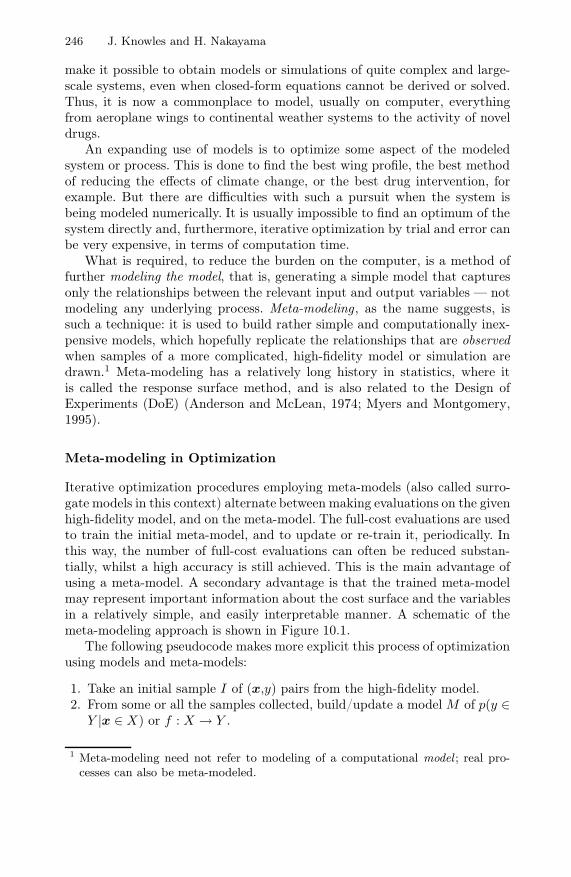
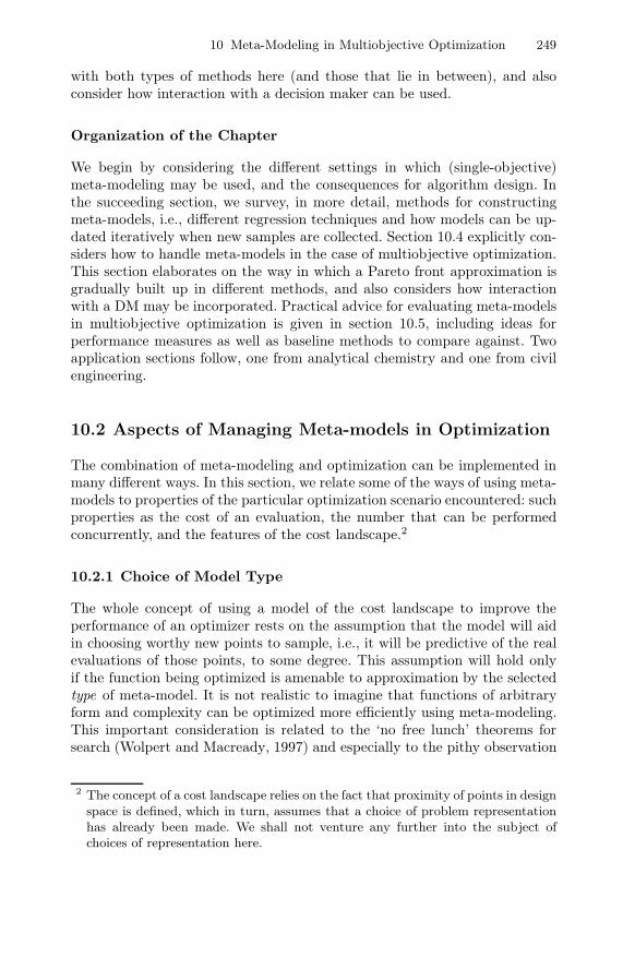
Iterative optimization procedures employing meta-models (also called surro-gate models in this context) alternate between making evaluations on the givenhigh-fidelity model, and on the meta-model. The full-cost evaluations are usedto train the initial meta-model, and to update or re-train it, periodically. Inthis way, the number of full-cost evaluations can often be reduced substan-tially, whilst a high accuracy is still achieved. This is the main advantage ofusing a meta-model. A secondary advantage is that the trained meta-modelmay represent important information about the cost surface and the variablesin a relatively simple, and easily interpretable manner. A schematic of themeta-modeling approach is shown in Figure 10.1.

The following pseudocode makes more explicit this process of optimizationusing models and meta-models:

1. Take an initial sample I of (x,y) pairs from the high-fidelity model.2. From some or all the samples collected, build/update a model M of p(y ∈

Y |x ∈ X) or f : X → Y .

1 Meta-modeling need not refer to modeling of a computational model ; real pro-cesses can also be meta-modeled.

10 Meta-Modeling in Multiobjective Optimization 247

parameters objectives

$$$

algorithm

12

6

metamodeliterative search

Fig. 10.1. A schematic diagram showing how meta-modeling is used for opti-mization. The high-fidelity model or function is represented as a black box, whichis expensive to use. The iterative searcher makes use of evaluations on both themeta-model and the black box function.

3. Using M , choose a new sample P of points and evaluate them on thehigh-fidelity model.

4. Until stopping criteria satisfied, return to 2.

The pseudocode is intentionally very general, and covers many different spe-cific strategies. For instance, in some methods the choice of new sample(s) Pis made solely based on the current model M , e.g. by finding the optimum onthe approximate model (cf. EGO, Jones et al. (1998) described in Section 3).Whereas, in other methods, P may be updated based on a memory of previ-ously searched or considered points: e.g. an evolutionary algorithm (EA) usinga meta-model may construct the new sample from its current population viathe usual application of variation operators, but M is then used to screen outpoints that it predicts will not have a good evaluation (see (Jin, 2005) andSection 4).

The criterion for selecting the next point(s) to evaluate, or for screening outpoints, is not always based exclusively on their predicted value. Rather, theestimated informativeness of a point may also be accounted for. This can be


estimated in different ways, depending on the form of the meta-model. Thereis a natural tension between choosing of samples because they are predicted tobe high-performance points and because they would yield much information,and this tension can be resolved in different ways.

The process of actually constructing a meta-model from data is related toclassical regression methods and also to machine learning. Where a model isbuilt up from an initial sample of solutions only, the importance of placingthose points in the design space in a theoretically well-founded manner is em-phasized, a subject dealt with in the classical design of experiments (DoE)literature. When the model is updated using new samples, classical DoE prin-ciples do not usually apply, and one needs to look to machine learning theoryto understand what strategies might lead to optimal performance. Here caremust be taken, however. Although the supervised learning paradigm is usu-ally taken as the default method used for training meta-models, it is worthnoting that in supervised learning, it is usually a base assumption that theavailable data for training a regression model are independent and identicallydistributed samples drawn from some underlying distribution. But in meta-modeling, the samples are not drawn randomly in this way: they are chosen,and this means that training sets will often contain highly correlated data,which can affect the estimation of goodness of fit and/or generalization per-formance. Also, meta-modeling in optimization can be related to active learn-ing (Cohn et al., 1996), since the latter is concerned with the iterative choice oftraining samples; however, active learning is concerned only with maximisingwhat is learned whereas meta-modeling in optimization is concerned mainly orpartially with seeking optima, so neither supervised learning or active learn-ing are identical with meta-modeling. Finally, in meta-modeling, samples areoften added to a ‘training set’ incrementally (see, e.g. (Cauwenberghs andPoggio, 2001)), and the model is re-trained periodically; how this re-trainingis achieved also leads to a variety of methods.

Interactive and Evolutionary Meta-modeling

Meta-modeling brings together a number of different fields to tackle the prob-lem of how to optimize expensive functions on a limited budget. Its basis inthe DoE literature gives the subject a classical feel, but evolutionary algo-rithms employing meta-models have been emerging for some years now, too(for a comprehensive survey, see(Jin, 2005)).

In the case of multiobjective problems, it does not seem possible or desir-able to make a clear distinction between interactive and evolutionary ap-proaches to meta-modeling. Some methods of managing and using meta-models seek to add one new search point, derived from the model, at everyiteration; others are closer to a standard evolutionary algorithm, with a pop-ulation of solutions used to generate a set of new candidate points, which arethen filtered using the model, so that only a few are really evaluated. We deal


with both types of methods here (and those that lie in between), and alsoconsider how interaction with a decision maker can be used.

Organization of the Chapter

We begin by considering the different settings in which (single-objective)meta-modeling may be used, and the consequences for algorithm design. Inthe succeeding section, we survey, in more detail, methods for constructingmeta-models, i.e., different regression techniques and how models can be up-dated iteratively when new samples are collected. Section 10.4 explicitly con-siders how to handle meta-models in the case of multiobjective optimization.This section elaborates on the way in which a Pareto front approximation isgradually built up in different methods, and also considers how interactionwith a DM may be incorporated. Practical advice for evaluating meta-modelsin multiobjective optimization is given in section 10.5, including ideas forperformance measures as well as baseline methods to compare against. Twoapplication sections follow, one from analytical chemistry and one from civilengineering.

10.2 Aspects of Managing Meta-models in Optimization

The combination of meta-modeling and optimization can be implemented inmany different ways. In this section, we relate some of the ways of using meta-models to properties of the particular optimization scenario encountered: suchproperties as the cost of an evaluation, the number that can be performedconcurrently, and the features of the cost landscape.2

10.2.1 Choice of Model Type

The whole concept of using a model of the cost landscape to improve theperformance of an optimizer rests on the assumption that the model will aidin choosing worthy new points to sample, i.e., it will be predictive of the realevaluations of those points, to some degree. This assumption will hold onlyif the function being optimized is amenable to approximation by the selectedtype of meta-model. It is not realistic to imagine that functions of arbitraryform and complexity can be optimized more efficiently using meta-modeling.This important consideration is related to the ‘no free lunch’ theorems forsearch (Wolpert and Macready, 1997) and especially to the pithy observation

2 The concept of a cost landscape relies on the fact that proximity of points in designspace is defined, which in turn, assumes that a choice of problem representationhas already been made. We shall not venture any further into the subject ofchoices of representation here.


of Thomas English that ‘learning is hard and optimization is easy in thetypical function’ (English, 2000).

In theory, given a cost landscape, there should exist a type of model thatapproximates it fastest as data is collected and fitting progresses. However,we think it is fair to say that little is yet known about which types of modelaccord best with particular features of a landscape and, in any case, verylittle may be known to guide this choice. Nonetheless, some basic consid-erations of the problem do help guide in the choice of suitable models andlearning algorithms. In particular, the dimension of the design space is im-portant, as certain models cope better than others with higher dimensions.For example, naive Bayes’ regression (Eyheramendy et al., 2003) is used rou-tinely in very high-dimensional feature spaces (e.g. in spam recognition whereindividual word frequencies form the input space). On the other hand, forlow-dimensional spaces, where local correlations are important, naive Bayes’might be very poor, whereas a Gaussian process model (Schwaighofer andTresp, 2003) might be expected to perform more effectively.

Much of the meta-modeling literature considers only problems over con-tinuous design variables, as these are common in certain engineering domains.However, there is no reason why this restriction need prevail. Meta-modelingwill surely become more commonly used for problems featuring discrete designspaces or mixed discrete and continuous variables. Machine learning methodssuch as classification and regression trees (C&RT) (Breiman, 1984), geneticprogramming (Langdon and Poli, 2001), and Bayes’ regression may be moreappropriate for modeling these high-dimensional landscapes than the splinesand polynomials that are used commonly in continuous design spaces. Meta-modeling of cost functions in discrete and/or high-dimensional spaces is byno means the only approach to combining machine learning and optimiza-tion, however. An alternative is to model the distribution over the variablesthat leads to high-quality points in the objective space — an approach knownas model-based search or estimation of distribution algorithms (Larranagaand Lozano, 2001; Laumanns and Ocenasek, 2002). The learnable evolutionmodel is a related approach (Michalski, 2000; Jourdan et al., 2005). Theseapproaches, though interesting rivals to meta-models, do not predict costs ormodel the cost function, and are thus beyond the scope of this chapter.

When choosing the type of model to use, other factors that are less linkedto properties of the cost landscape/design space should also be considered.Models differ in how they scale in terms of accuracy and speed of trainingas the number of training samples varies. Some models can be trained in-crementally, using only the latest samples (some particular SVMs), whereasothers (most multi-layer perceptrons) can suffer from ‘catastrophic forgetting’if trained on new samples only, and need to use complete re-training over allsamples when some new ones become available, or some other strategy of re-hearsal(Robins, 1997). Some types of model need cross-validation to controloverfitting, whereas others use regularization. Finally, some types of model,such as Gaussian random fields, model their own error, which can be a distinct


advantage when deciding where to sample next (Jones et al., 1998; Emmerichet al., 2006). A more detailed survey of types of model, and methods for train-ing them, is given in section 3.

10.2.2 The Cost of Evaluations

One of the most important aspects affecting meta-modeling for optimizationis the actual cost of an evaluation. At one extreme, a cost function may onlytake the order of 1s to evaluate, but is still considered expensive in the contextof evolutionary algorithm searches where tens of thousands of evaluations aretypical. At the other extreme, when the design points are very expensive,such as vehicle crash tests (Hamza and Saitou, 2005), then each evaluationmay be associated with financial costs and/or may take days to organize andcarry out. In the former case, there is so little time between evaluations thatmodel-fitting is best carried out only periodically (every few generations ofthe evolutionary algorithm) and new sample points are generated mainly asa result of the normal EA mechanisms, with the meta-model playing only asubsidiary role of filtering out estimated poor points. In the latter case, theoverheads of fitting and cross-validating models is small compared with thetime between evaluations, so a number of alternative models can be fitted andvalidated after every evaluation, and might be used very carefully to decideon the best succeeding design point, e.g. by searching over the whole designspace using the meta-model(s) to evaluate points.

The cost of evaluations might affect the meta-modeling strategy in morecomplicated and interesting ways than the simple examples above, too. Insome applications, the cost of evaluating a point is not uniform over the designspace, so points may be chosen based partly on their expected cost to evaluate(though this has not been considered in the literature, to our knowledge). Inother applications, the cost of determining whether a solution is feasible ornot is expensive, while evaluating it on the objective function is cheap. Thiswas the case in (Joslin et al., 2006), and led to a particular strategy of onlychecking the constraints for solutions passing a threshold on the objectivefunction.

In some applications, the cost of an evaluation can be high in time, yetmany can be performed in parallel. This situation occurs, for example, in usingoptimization to design new drugs via combinatorial chemistry methods. Here,the time to prepare a drug sample and to test it can be of the order of 24hours, but using high-throughput equipment, several hundred or thousandsof different drug compounds can be made and tested in each batch (Corneet al., 2002). Clearly, this places very particular constraints on the meta-modeling/optimization process: there is not always freedom to choose howfrequently updates of the model are done, or how many new design pointsshould be evaluated in each generation. Only future studies will show how tobest deal with these scenarios.


10.2.3 Advanced Topics

Progress in meta-modeling seems to be heading in several exciting new direc-tions, worth mentioning here.

Typically, when fitting a meta-model to the data, a single global model islearned or updated, using all available design points. However, some researchis departing from this by using local models (Atkeson et al., 1997), which aretrained only on local subsets of the data (Emmerich et al., 2006). Anotherdeparture from the single global model is the possibility of using an ensembleof meta-models (Hamza and Saitou, 2005). Ensemble learning has generaladvantages in supervised learning scenarios (Brown et al., 2005) and mayincrease the accuracy of meta-models too. Moreover, Jin and Sendhoff (2004)showed that ensemble methods can be used to predict the quality of theestimation, which can be very useful in the meta-modeling approach.

Noise or stochasticity is an element in many systems that require optimiza-tion. Many current meta-modeling methods, especially those based on radialbasis functions or Kriging (see next section) assume noiseless evaluation, sothat the uncertainty of the meta-model at the evaluated points is assumedto be zero. However, with noisy functions, to obtain more accurate estimatesof the expected quality of a design point, several evaluations may be needed.Huang et al. (2006) consider how to extend the well-known EGO algorithm(see next section) to account for the case of noise or stochasticity on the ob-jective function. Other noisy optimization methods, such as those based onEAs (Fieldsend and Everson, 2005), could be combined with meta-models infuture work.

A further exciting avenue of research is the use of transductive learning.It has been shown by Chapelle et al. (1999) that in supervised learning of aregression model, knowledge of the future test points (just in design space),at the time of training, can be used to improve the training and lead to betterultimate prediction performance on those points. This results has been im-ported into meta-modeling by Schwaighofer and Tresp (2003), which comparestransductive Gaussian regression methods with standard, inductive ones, andfinds them much more accurate.

10.3 Brief Survey of Methods for Meta-modeling

The Response Surface Method (RSM) is probably the most widely applied tometa-modeling (Myers and Montgomery, 1995). The role of RSM is to predictthe response y for the vector of design variables x ∈ Rn on the basis of thegiven sampled obsevation (xi, yi) (i = 1, . . . , p).

Usually, the Response Surface Method is a generic name, and it coversa wide range of methods. Above all, methods using experimental design arefamous. However, many of them select sample points only on the basis of


statisitical analysis of design variable space. They may provide a good ap-proximation of black-box functions with a mild nonlineality. It is clear, how-ever, that in cases in which the black-box function is highly nonlinear, wecan obtain better performance by methods taking into account not only thestatistical property of design variable space but also that of range space ofthe black-box function (in other words, the shape of function).

Moreover, machine learning techniques such as RBF (Radial Basis Func-tion) networks and Support Vector Machines (SVM) have been recently ap-plied for approximating the black-box function (Nakayama et al., 2002, 2003).

10.3.1 Using Design of Experiments

Suppose, for example for simplicitly, that we consider a response functiongiven by a quadratic polynomial:

y = β0 +n∑

i=1

βixi +n∑

i=1

βiix2i +

∑

i<j

βijxixj (10.1)

Since the above equation is linear with respect to βi, we can rewrite theequation (10.1) into the following:

y = Xβ + ε, (10.2)

where E(ε) = 0, V (ε) = σ2I.The above (10.2) is well known as linear regression, and the solution β

minimizing the squarred error is given by

β = (XT X)−1XT y (10.3)

The variance covariance matrix V (β) = cov(βi, βj) of the least squarred errorprediction β given by (10.3) becomes

V (β) = cov(βi, βj) = E((β − E(β))(β − E(β)) (10.4)= (XT X)−1σ2, (10.5)

where σ2 is the variance of error in the response y such that E(εεT ) = σ2I.

i) Orthogonal DesignOrthogonal design is usually applied for experimental design with linear poly-nomials. Selecting sample points in such a way that the set X is orthogonal,the matrix XT X becomes diagonal. It is well known that the orthogonal de-sign with the first order model is effective for cases with only main effectsor first order interaction effects. For the polynomial regressrion with higherorder (≥ 2), orthogonal polynomials are usually used in order to make the


design to be orthogonal (namely, XT X is diagonal). Then the coefficients ofpolynomials are easily evaluated by using orthogonal arrays.

Another kind of experimental design, e.g., CCD (Cetral Composite De-sign) is applied mostly for experiments with quadratic polynomials.

ii) D-optimalityConsidering the equation (10.5), the matrix (XT X)−1 should be minimizedso that the variance of the predicted β may decrease. Since each element of(XT X)−1 has det(XT X) in the denomnator, we can expect to decrease notonly variance but also covariance of βi by maximizing det(XT X). This is theidea of D-optimality in design of experiments. In fact, it is usual to use themoment matrix

M =XT X

p, (10.6)

where p is the number of sample points.Other criteria are possible: to minimize the trace of (XT X)−1 (A-

optimiality), to minimize the maximal value of the diagonal components of(XT X)−1 (minimax criterion), to maximize the minimal eigen value of XT X(E-optimality). In general, however, the D-optimality criterion is widely usedfor many practical problems.

10.3.2 Kriging Method

Consider the response y(x) as a realization of a random function, Y (x) suchthat

Y (x) = µ(x) + Z(x). (10.7)

Here, µ(x) is a global model and Z(x) reflecting a deviation from the globalmodel is a random function with zero mean and nonzero covariance given by

cov[Z(x), Z(x′)] = σ2R(x, x′) (10.8)

where R is the correlation between Z(x) and Z(x′). Usually, the stochas-tic process is supposed to be stationary, which implies that the correlationR(x, x′) depends only on x− x′, namely

R(x, x′) = R(x− x′). (10.9)

A commonly used example of such correlation functions is

R(x, x′) = exp[−n∑

i=1

θi|xi − x′i|2], (10.10)

where xi and x′i are i-th component of x and x′, respectively.

Although a linear regressrion model∑k

j=1 µjfj(x) can be applied as aglobal model in (10.7) (universal Kriging), µ(x) = µ in which µ is unknown


but constant is commonly used in many cases (ordinary Kriging). In the or-dinary Kriging, the best linear unbiased predictor of y at an untried x can begiven by

y(x) = µ + rT (x)R−1(y − 1µ), (10.11)

where µ = (1T R−11)−11T R−1y is the generalized least squares estimator ofµ, r(x) is the n×1 vector of correlations R(x, xi) between Z at x and sampledpoints xi (i = 1, . . . , p), R is an n× n correlation matrix with (i, j)-elementdefined by R(xi, xj) and 1 is a unity vector whose components are all 1.

Using Expected Improvement

Jones et al. (1998) suggested a method called EGO (Efficient Global Opti-mization) for black-box objective functions. They applied a stochastic processmodel (10.7) for predictor and the expected improvement as a figure of meritfor additional sample points.

The estimated value of the mean of the stochastic process, µ, is given by

µ =1T R−1y

1T R−11. (10.12)

In this event, the variation σ2 is estimated by

σ2 =(y − 1µ)T R−1(y − 1µ)

n. (10.13)

The mean squared error of the predictor is estimated by

s2(x) = σ2[1− rT R−1r +(1 − 1T R−1r)2

1T R−11]. (10.14)

In the following s =√

s2(x) is called a standard error.Using the above predictor on the basis of stochastic process model, Jones

et al. applied the expected improvemnet for adding a new sample point. Letfpmin = min{y1, . . . , yp} be the current best function value. They model the

uncertainty at y(x) by treating it as the realization of a normally distributedrandom variable Y with mean and standard deviation given by the abovepredictor and its standard error.

For minimization cases, the improvement at x is I = [max(fpmin − Y, 0).

Therefore, the expected improvement is given by

E[I(x)] = E[max(fpmin − Y, 0)].

It has been shown that the above formula can be expanded as follows:

E(I) ={

(fpmin − y)Φ(fp

min−y

s ) + sφ(fpmin−y

s ) if s < 00 if s = 0,

(10.15)


where φ is the standard normal density and Φ is the distribution function.We can add a new sample point which maximizes the expected improve-

ment. Although Jones et al. proposed a method for maximizing the expectedimprovement by using the branch and bound method, it is possible to selectthe best one among several candidates which are generated randomly in thedesign variable space.

Furthermore, Schonlau (1997) extended the expected improvement as fol-lows: Letting Ig = max((fp

min − Y )g, 0), then

E(Ig) = sg

g∑

i=0

(−1)i(g!

i!(g − i)!)( ´fp

min)g−iTi (10.16)

where´fp

min =fp

min − y

sand

Tk = −φ( ´fpmin)( ´fp

min)(k−1) + (k − 1)Tk−2.

HereT0 = Φ( ´fp

min)

T1 = −φ( ´fpmin).

It has been observed that larger value of g makes the global search, whilesmaller value of g the local search. Therefore, we can control the value of gdepending upon the situation.

10.3.3 Computational Intelligence

Multi-layer Perceptron Neural Networks

The multi-layer perceptron (MLP) is used in several meta-modeling appli-cations in the literature (Jin et al., 2001; Gaspar-Cunha and Vieira, 2004).It is well-known that MLPs are universal approximators, which makes themattractive for modeling black box functions for which little information abouttheir form is known. But, in practice, it can be difficult and time-consumingto train MLPs effectively as they still have biases and it is easy to get caughtin local minima which give far from desirable performance. A large MLP withmany weights has a large capacity, i.e. it can model complex functions, butit is also easy to over-fit it, so that generalization performance may be poor.The use of a regularization term to help control the complexity is necessary toensure better generalization performance. Cross-validation can also be usedduring the training to mitigate overfitting.

Disadvantages of using MLPs may include the difficulty to train it quickly,especially if cross-validation with several folds is used (a problem in some ap-plications). It is not easy to train incrementally (compare with RBFs). More-over, an MLP does not estimate its own error (compare with Kriging), whichmeans that it can be difficult to estimate the best points to sample next.


Radial Basis Function Networks

Since the number of sample points for predicting objective functions shouldbe as few as possible, incremental learning techniques which predict black-box functions by adding learning samples step by step, are attractive. RBFNetworks (RBFN) and Support Vector Machines (SVM) are effective to thisend. For RBFN, the necessary information for incremental learning can beeasily updated, while the information of support vector can be utilized inselecting additional samples as the sensitivity in SVM. The details of theseapproaches can be seen in (Nakayama et al., 2002) and (Nakayama et al.,2003). Here, we introduce the incremental learning by RBFN briefly in thefollowing.

The output of an RBFN is given by

f(x) =m∑

j=1

wjhj(x),

where hj , j = 1, . . . , m are radial basis functions, e.g.,

hj(x) = e−‖x−cj‖2/rj .

Given the training data (xi, yi), i = 1, · · · , p, the learning of RBFN is usuallymade by solving

min E =p∑

i=1

(yi − f(xi))2 +m∑

j=1

λjw2j

where the second term is introduced for the purpose of regularization.In general cases with a large number of training data p, the number of basis

functions m is set to be less than p in order to avoid overlearning. However,the number of training data is not so large in this paper, because it is desiredto be as small as possible in applications under consideration. The value m isset, therefore, to be equal to p in later sections in this paper. Also, the centerof radial basis function ci is set to be xi. The values of λj and rj are usuallydetermined by cross-validation test. It is observed through our experience thatin many problems we have a good performance with λj = 0.01 and a simpleestimate for rj given by

r =dmax

n√

np, (10.17)

where dmax is the maximal distance among the data; n is the dimension ofdata; p is the number of data.

Letting A = (HTp Hp + Λ), we have

Aw = HTp y,

as a necessary condition for the above minimization. Here


HTp = [h1 · · · hp] ,

where hTj = [h1(xj), . . . , hm(xj)], and Λ is a diagonal matrix whose diagonal

components are λ1 · · · λm.Therefore, the learning in RBFN is reduced to finding

A−1 = (HTp Hp + Λ)−1.

The incremental learning in RBFN can be made by adding new samplesand/or a basis function, if necesary. Since the learning in RBFN is equiva-lent to the matrix inversion A−1, the additional learning here is reduced tothe incremental calculation of the matrix inversion. The following algorithmcan be seen in (Orr, 1996):

(i) Adding a New Training SampleAdding a new sample xp+1, the incremental learning in RBFN can be madeby the following simple update formula: Let

Hp+1 =[

Hp

hTp+1

]

,

where hTp+1 = [h1(xp+1), . . . , hm(xp+1)].

Then

A−1p+1 = A−1

p − A−1p hp+1h

Tp+1A

−1p

1 + hTp+1A

−1p hp+1

.

(ii) Adding a New Basis FunctionIn those cases where a new basis function is needed to improve the learningfor a new data, we have the following update formula for the matrix inversion:Let

Hm+1 =[Hm hm+1

],

where hTm+1 = [hm+1(x1), . . . , hm+1(xp)].

ThenA−1

m+1 =[

A−1m 0

0T 0

]

+1

λm+1 + hTm+1(Ip −HmA−1

m HTm)hm+1

×[A−1

m HTmhm+1

−1

][A−1

m HTmhm+1

−1

]T

.

10.3.4 Support Vector Machines

Support vector machines (SVMs) were originally developed for pattern clas-sification and later extended to regression (Cortes and Vapnik, 1995; Vapnik,1998; Cristianini and Shawe-Tylor, 2000; B.Schölkopf and A.J.Smola, 2002).Regression using SVMs, called often support vector regression, plays an im-portant role in meta-modeling. However, the essential idea of support vector


regression lies in SVMs for classification. Therefore, we start with a brief re-view of SVM for classification problems.

Let X be a space of conditional attributes. For binary classification prob-lems, the value of +1 or −1 is assigned to each pattern xi ∈ X accordingto its class A or B. The aim of machine learning is to predict which classnewly observed patterns belong to on the basis of the given training data set(xi, yi) (i = 1, . . . , p), where yi = +1 or −1. This is performed by finding adiscriminant function f(x) such that f(x) � 0 for x ∈ A and f(x) < 0 forx ∈ B. Linear discriminant functions, in particular, can be expressed by thefollowing linear form

f(x) = wT x + b

with the property

wT x + b � 0 for x ∈ AwT x + b < 0 for x ∈ B.

In cases where training data set X is not linearly separable, we map theoriginal data set X to a feature space Z by some nonlinear map φ. Increasingthe dimension of the feature space, it is expected that the mapped data setbecomes linearly separable. We try to find linear classifiers with maximalmargin in the feature space. Letting zi = φ(xi), the separating hyperplanewith maximal margin can be given by solving the following problem with thenormalization wT z + b = ±1 at points with the minimum interior deviation:

minw,b

||w|| (SVMhard)P

s.t. yi

(wT zi + b

)� 1, i = 1, . . . , p.

Dual problem of (SVMhard)P with 12 ||w||22 is

maxαi

p∑

i=1

αi − 12

p∑

i,j=1

αiαjyiyjφ(xi)T φ(xj) (SVMhard)D

s.t.p∑

i=1

αiyi = 0,

αi � 0, i = 1, . . . , p.

Using the kernel function K(x, x′) = φ(x)T φ(x′), the problem (SVMhard)D

can be reformulated as follows:

maxαi

p∑

i=1

αi − 12

p∑

i,j=1

αiαjyiyjK(xi, xj) (SVMhard)

s.t.p∑

i=1

αiyi = 0,

αi � 0, i = 1, . . . , p.


Although several kinds of kernel functions have been suggested, the Gaussiankernel

K(x, x′) = exp(

−||x− x′||22r2

)

is popularly used in many cases.

MOP/GP Approaches to Support Vector Classification

In 1981, Freed and Glover suggested to get just a hyperplane separating twoclasses with as few misclassified data as possible by using goal programming(Freed and Glover, 1981) (see also (Erenguc and Koehler, 1990)). Let ξi denotethe exterior deviation which is a deviation from the hyperplane of a point xi

improperly classified. Similarly, let ηi denote the interior deviation which is adeviation from the hyperplane of a point xi properly classified. Some of mainobjectives in this approach are as follows:

i) Minimize the maximum exterior deviation (decrease errors asmuch as possible)

ii) Maximize the minimum interior deviation (i.e., maximize the mar-gin)

iii) Maximize the weighted sum of interior deviation

iv) Minimize the weighted sum of exterior deviation.

Introducing the idea iv) above, the well known soft margin SVM with slackvariables (or, exterior deviations) ξi (i = 1, . . . , p) which allow classificationerrors to some extent can be formulated as follows:

minw,b,ξi

12||w||22 + C

p∑

i=1

ξi (SVMsoft)P

s.t. yi

(wT zi + b

)� 1− ξi,

ξi � 0, i = 1, . . . , p,

where C is a trade-off parameter between minimizing ||w||22 and minimizing∑pi=1 ξi.

Using a kernel function in the dual problem yields

maxαi

p∑

i=1

αi − 12

p∑

i,j=1

αiαjyiyjK(xi, xj) (SVMsoft)

s.t.p∑

i=1

αiyi = 0,

0 � αi � C, i = 1, . . . , p.


Lately, taking into account the objectives (ii) and (iv) of goal programming,we have the same formulation of ν-support vector algorithm developed bySchölkopf and Smola (1998):

minw,b,ξi,ρ

12||w||22 − νρ +

1p

p∑

i=1

ξi (ν−SVM)P

s.t. yi

(wT zi + b

)� ρ− ξi,

ρ � 0, ξi � 0, i = 1, . . . , p,

where 0 � ν � 1 is a parameter.Compared with the existing soft margin algorithm, one of the differences is

that the parameter C for slack variables does not appear, and another differ-ence is that the new variable ρ appears in the above formulation. The problem(ν−SVM)P maximizes the variable ρ which corresponds to the minimum inte-rior deviation (i.e., the minimum distance between the separating hyperplaneand correctly classified points).

The Lagrangian dual problem to the problem (ν−SVM)P is as follows:

maxαi

− 12

p∑

i,j=1

yiyjαiαjK (xi, xj) (ν−SVM)

s.t.p∑

i=1

yiαi = 0,

�∑

i=1

αi � ν,

0 � αi � 1p, i = 1, . . . , p.

Other variants of SVM considering both slack variables for misclassified datapoints (i.e., exterior deviations) and surplus variables for correctly classifieddata points (i.e., interior deviations) are possible (Nakayama and Yun, 2006a):Considering iii) and iv) above, we have the fomula of total margin SVM, whileν−SVM can be derived from i) and iii).

Finally, µ−ν−SVM is derived by considering the objectives i) and ii) inMOP/GP:

minw,b,ρ,σ

12‖w‖22 − νρ + µσ (µ− ν−SVM)P

s.t. yi

(wT zi + b

)� ρ− σ, i = 1, . . . , p,

ρ � 0, σ � 0,

where ν and µ are parameters.The dual formulation is given by


maxαi

− 12

p∑

i,j=1

αiαjyiyjK (xi, xj) (µ− ν−SVM)

s.t.p∑

i=1

αiyi = 0,

ν �p∑

i=1

αi � µ,

αi � 0, i = 1, . . . , p.

Letting α∗ be the optimal solution to the problem (µ−ν−SVM), the offset b∗

can be chosen easily for any i satisfying α∗i > 0. Otherwise, b∗ can be obtained

by the similar way with the decision of the b∗ in the other algorithms.

Support Vector Regression

Support Vector Machines were extended to regression by introducing the εinsensitive loss function by Vapnik (1998). Denote the given sample data by(xi, yi) for i = 1, ..., p. Suppose that the regression function on the Z space

is expressed by f(z) =p∑

i=1

wizi + b. The linear ε insensitive loss function is

defined by

Lε(z, y, f) = |y − f(z)|ε = max(0, |y − f(z)| − ε).

For a given insensitivity parameter ε,

minw,b,ε,ξi,ξi

12‖w‖22 + C

(1p

p∑

i=1

(ξi + ξi))

(soft−SVR)P

s.t.(wT zi + b

)− yi � ε + ξi, i = 1, . . . , p,

yi −(wT zi + b

)� ε + ξi, i = 1, . . . , p,

ε, ξi, ξi � 0

where C is a trade-off parameter between the norm of w and ξ (ξ).The dual formulation to (soft−SVR)P is given by


maxαi,αi

− 12

p∑

i,j=1

(αi − αi) (αj − αj) K (xi, xj) (soft−SVR)

+p∑

i=1

(αi − αi) yi − ε

p∑

i,j=1

(αi + αi)

s.t.p∑

i=1

(αi − αi) = 0,

0 � αi � C

p, 0 � αi � C

p, i = 1, . . . , p.

In order to decide ε automatically, Schölkopf and Smola proposed ν-SVR asfollows (Schölkopf and Smola, 1998):

minw,b,ε,ξi,ξi

12‖w‖22 + C

(νε +

1p

p∑

i=1

(ξi + ξi))

(ν−SVR)P

s.t.(wT zi + b

)− yi � ε + ξi, i = 1, . . . , p,

yi −(wT zi + b

)� ε + ξi, i = 1, . . . , p,

ε, ξi, ξi � 0,

where C and ν are trade-off parameters between the norm of w and ε andξi (ξi).

The dual formulation to (ν−SVR)P is given by

maxαi,αi

− 12

p∑

i,j=1

(αi − αi) (αj − αj)K (xi, xj) (ν−SVR)

+p∑

i=1

(αi − αi) yi

s.t.p∑

i=1

(αi − αi) = 0,

p∑

i=1

(αi + αi) � C · ν,

0 � αi � C

p, 0 � αi � C

p, i = 1, . . . , p.

In a similar fashion to classification, we can obtain (µ− ν−SVR) as follows:


minw,b,ε,ξ,ξ

12‖w‖22 + νε + µ(ξ + ξ) (µ− ν−SVR)P

s.t.(wT zi + b

)− yi � ε + ξ, i = 1, . . . , p,

yi −(wT zi + b

)� ε + ξ, i = 1, . . . , p,

ε, ξ, ξ � 0,

where ν and µ are trade-off parameters between the norm of w and ε and ξ.The dual formulation of µ− ν−SVR is as follows:

maxαi,αi

− 12

p∑

i,j=1

(αi − αi) (αj − αj)K (xi, xj) (µ− ν−SVR)

+p∑

i=1

(αi − αi) yi

s.t.p∑

i=1

(αi − αi) = 0,

p∑

i=1

αi � µ,

p∑

i=1

αi � µ,

p∑

i=1

(αi + αi) � ν,

αi � 0, αi � 0, i = 1, . . . , p.

10.4 Managing Meta-models of Multiple Objectives

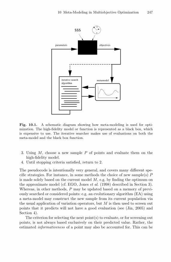
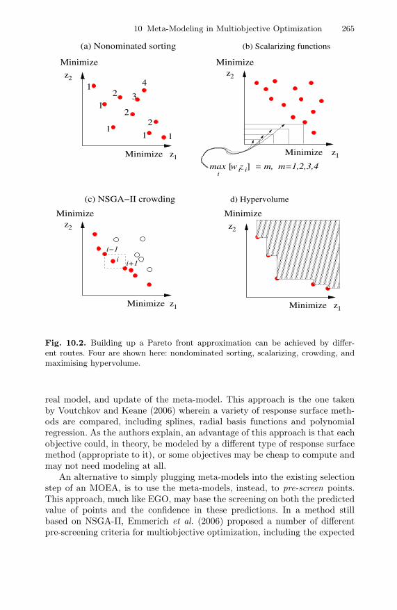
Meta-modeling in the context of multiobjective optimization has been consid-ered in several works in recent years (Chafekar et al., 2005; Emmerich et al.,2006; Gaspar-Cunha and Vieira, 2004; Keane, 2006; Knowles, 2006; Nain andDeb, 2002; Ray and Smith, 2006; Voutchkov and Keane, 2006). The gener-alization to multiple objective functions has led to a variety of approaches,with differences in what is modeled, and also how models are updated. Thesedifferences follow partly from the different possible methods that there are ofbuilding up a Pareto front approximation (see Figure 10.2).

In a modern multiobjective evolutionary algorithm approach like NSGA-II, selection favours solutions of low dominance rank and uncrowded solu-tions, which helps build up a diverse and converged Pareto set approximation.A straightforward way to obtain a meta-modeling-based multiobjective opti-mization algorithm is thus to take NSGA-II and simply plug in meta-models ofeach independent objective function. This can be achieved by running NSGA-II for several generations on the meta-model (initially constructed from aDoE sample), and then cycling through phases of selection, evaluation on the


��

��

1

z2

= m, m=1,2,3,4i ii

max w z [ ]

Minimize z

Minimize

Minimize z1

z2

d) Hypervolume

z1

z2

i−1

i+1i

(c) NSGA−II crowding

Minimize

Minimize z1

z2

1

1

11

2

4

2

3

1

2

(a) Nonominated sorting (b) Scalarizing functions

Minimize

Minimize

Minimize

Fig. 10.2. Building up a Pareto front approximation can be achieved by differ-ent routes. Four are shown here: nondominated sorting, scalarizing, crowding, andmaximising hypervolume.

real model, and update of the meta-model. This approach is the one takenby Voutchkov and Keane (2006) wherein a variety of response surface meth-ods are compared, including splines, radial basis functions and polynomialregression. As the authors explain, an advantage of this approach is that eachobjective could, in theory, be modeled by a different type of response surfacemethod (appropriate to it), or some objectives may be cheap to compute andmay not need modeling at all.

An alternative to simply plugging meta-models into the existing selectionstep of an MOEA, is to use the meta-models, instead, to pre-screen points.This approach, much like EGO, may base the screening on both the predictedvalue of points and the confidence in these predictions. In a method stillbased on NSGA-II, Emmerich et al. (2006) proposed a number of differentpre-screening criteria for multiobjective optimization, including the expected


improvement and the probability of improvement. Note that in the case ofmultiobjective optimization, improvement is relative to the whole Pareto setapproximation achieved so far, not a single value. Thus, to measure improve-ment, the estimated increase in hypervolume (Zitzler et al., 2003) of the cur-rent approximation set (were a candidate point added to it) is used, based on ameta-model for each objective function. In experiments, Emmerich et al com-pared four different screening criteria on two and three-objective problems,and found improvement over the standard NSGA-II in all cases.

The approach of Emmerich et al is a sophisticated method of generalizingthe use of meta-models to multiobjective optimization, via MOEAs, thoughit is as yet open whether this sophistication leads to better performance thanthe simpler method of Voutchkov and Keane (2006). Moreover, it does seemslightly unnatural to marry NSGA-II, which uses dominance rank and crowd-edness to select its ‘parents’, with a meta-modeling approach that uses thehypervolume to estimate probable improvement. It would seem more logicalto use evolutionary algorithms that themselves maximize hypervolume as thefitness assignment method, such as (Emmerich et al., 2005). It remains to beseen whether such approaches would perform even better.

One worry with the methods described so far is that fitness assignmentsbased on dominance rank (like NSGA-II) can perform poorly when the numberof objectives is greater than three or four (Hughes, 2005). Hypervolume maybe a better measure but it is very expensive to compute for large dimension,as the complexity of known methods for computing it is polynomial in the setsize but exponential in d. Thus, scaling up objective dimension in methodsbased on either of the approaches described above might prove difficult.

A method that does not use either hypervolume or dominance rank is theParEGO approach proposed by Knowles (2006). This method is a generaliza-tion to multiobjective optimization of the well-founded EGO algorithm (Joneset al., 1998). To build up a Pareto front, ParEGO uses a series of weightingvectors to scalarize the objective functions. At each iteration of the algorithm,a new candidate point is determined by (i) computing the expected improve-ment (Jones et al., 1998) in the ‘direction’ specified by the weighting vectordrawn for that iteration, and (ii) searching for a point that maximizes thisexpected improvement (a single-objective evolutionary algorithm is used forthis search). The use of such scalarizing weight vectors has been shown toscale well to many objectives, compared with Pareto ranking (Hughes, 2005).The ParEGO method has the additional advantage that it would be relativelystraightforward to make it interactive, allowing the user to narrow down theset of scalarizing weight vectors to allow focus on a particular region of thePareto front. This can further reduce the number of function evaluations it isnecessary to perform.

Yet a further way of building up a Pareto front is exemplified in the finalmethod we review here. (Chafekar et al., 2005) proposes a genetic algorithmwith meta-models OEGADO, based closely on their own method for singleobjective optimization. To make it work for the multiobjective case, a dis-


tinct genetic algorithm is run for each objective, with information exchangeoccurring between the algorithms at intervals, which helps the GAs to find thecompromise solutions. The fact that each objective is optimized by its owngenetic algorithm means that objective functions with different computationaloverhead can be appropriately handled — slow objectives do not slow downthe evaluation of faster ones. The code may also be trivially implemented onparallel architectures.

10.4.1 Combining Interactive Methods and EMO for Generating aPareto Frontier

Aspiration Level Methods for Interactive MultiobjectiveProgramming

Since there may be many Pareto solutions in practice, the final decision shouldbe made among them taking the total balance over all criteria into account.This is a problem of value judgment of DM. The totally balancing over criteriais usually called trade-off. Interactive multiobjective programming searches asolution in an interactive way with DM while making trade-off analysis on thebasis of DM’s value judgment. Among them, the aspiration level approach isnow recognized to be effective in practice, because

(i) it does not require any consistency of DM’s judgment,(ii) aspiration levels reflect the wish of DM very well,(iii)aspiration levels play the role of probe better than the weight for objective

functions.

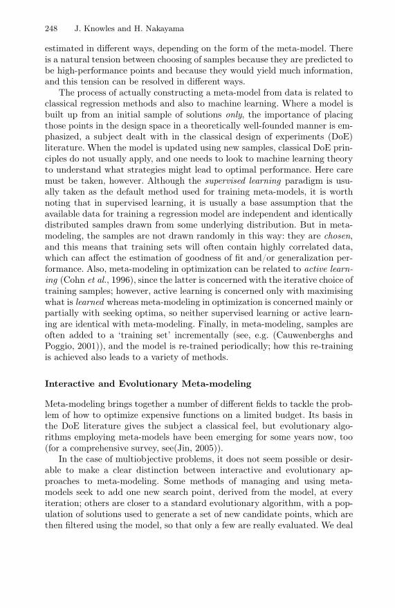
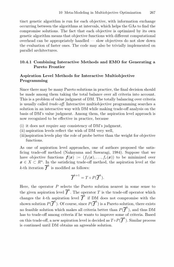
As one of aspiration level approaches, one of authors proposed the satis-ficing trade-off method (Nakayama and Sawaragi, 1984). Suppose that wehave objective functions f(x) := (f1(x), . . . , fr(x)) to be minimized overx ∈ X ⊂ Rn. In the satisficing trade-off method, the aspiration level at thek-th iteration f

kis modified as follows:

fk+1

= T ◦ P (fk).

Here, the operator P selects the Pareto solution nearest in some sense tothe given aspiration level f

k. The operator T is the trade-off operator which

changes the k-th aspiration level fk

if DM does not compromise with theshown solution P (f

k). Of course, since P (f

k) is a Pareto solution, there exists

no feasible solution which makes all criteria better than P (fk), and thus DM

has to trade-off among criteria if he wants to improve some of criteria. Basedon this trade-off, a new aspiration level is decided as T ◦P (f

k). Similar process

is continued until DM obtains an agreeable solution.


On the Operation P

The operation which gives a Pareto solution P (fk) nearest to f

kis per-

formed by some auxiliary scalar optimization. It has been shown in Sawaragi-Nakayama-Tanino (1985) that the only one scalarization technique, whichprovides any Pareto solution regardless of the structure of problem, is of theTchebyshev norm type. However, the scalarization function of Tchebyshevnorm type yields not only a Pareto solution but also a weak Pareto solution.Since weak Pareto solutions have a possibility that there may be another solu-tion which improves a criteria while others being fixed, they are not necessarily“efficient" as a solution in decision making. In order to exclude weak Paretosolutions, the following scalarization function of the augmented Tchebyshevtype can be used:

max1�i�r

ωi

(fi(x)− f i

)+ α

r∑

i=1

ωifi(x), (10.18)

where α is usually set a sufficiently small positive number, say 10−6.The weight ωi is usually given as follows: Let f∗

i be an ideal value which isusually given in such a way that f∗

i < min {fi(x) | x ∈ X}. For this circum-stance, we set

ωki =

1

fk

i − f∗i

. (10.19)

The minimization of (10.18) with (10.19) is usually performed by solving thefollowing equivalent optimization problem, because the original one is notsmooth:

(AP) minimizez, x

z + α

r∑

i=1

ωifi(x)

subject to ωki

(fi(x)− f

k

i

)� z (10.20)

x ∈ X.

On the Operation T

In cases that DM is not satisfied with the solution for P (fk), he/she is re-

quested to answer his/her new aspiration level fk+1

. Let xk denote the Paretosolution obtained by projection P (f

k), and classify the objective functions

into the following three groups:

(i) the class of criteria which are to be improved more,(ii) the class of criteria which may be relaxed,(iii)the class of criteria which are acceptable as they are.


*f

2f

1f

k

f

ˆ kf

1ˆ k �

f1k �

f

Fig. 10.3. Satisficing Trade-off Method

Let the index set of each class be denoted by IkI , Ik

R, IkA, respectively. Clearly,

fk+1

i < fi(xk) for all i ∈ IkI . Usually, for i ∈ Ik

A, we set fk+1

i = fi(xk). Fori ∈ Ik

R, DM has to agree to increase the value of fk+1

i . It should be notedthat an appropriate sacrifice of fj for j ∈ Ik

R is needed for attaining theimprovement of fi for i ∈ Ik

I .

Combining Satisficing Trade-off Method and SequentialApproximate Optimization

Nakayama and Yun proposed a method combining the satisficing trade-offmethod for interactive multiobjective programming and the sequential ap-proximate optimization using µ− ν−SVR (Nakayama and Yun, 2006b). Theprocedure is summarized as follows:

Step 1. (Real Evaluation)Evaluate actually the values of objective functions f(x1), f(x2), . . . , f(x�)for sampled data x1, . . . , x� through computational simulation analysis orexperiments.

Step 2. (Approximation)Approximate each objective function f1(x), . . . , fm(x) by the learning ofµ− ν−SVR on the basis of real sample data set.

Step 3. (Find a Pareto Solution Nearest to the Aspiration Leveland Generate Pareto Frontier)

Find a Pareto optimal solution nearest to the given aspiration level forthe approximated objective functions f(x) := (f1(x), . . . , fm(x)). This isperformed by using GA for minimizing the augmented Tchebyshev scalar-ization function (10.18). In addition, generate Pareto frontier by MOGAfor accumulated individuals during the procedure for optimizing the aug-mented Tchebyshev scalarization function.

Step 4. (Choice of Additional Learning Data)Choose the additional �0-data from the set of obtained Pareto optimalsolutions. Go to Step 1. (Set �← � + �0.)


how to choose the additional data

Stage 0. First, add the point with highest achievement degreeamong Pareto optimal solutions obtained in Step 3. (← localinformation)

Stage 1. Evaluate the ranks for the real sampled data of Step 1by the ranking method (Fonseca and Fleming, 1993).

Stage 2. Approximate the rank function associated with theranks calculated in the Stage 1 by µ− ν−SVR.

Stage 3. Calculate the expected fitness for Pareto optimal so-lutions obtained in Step 3.

Stage 4. Among them, add the point with highest rank. (←globalinformation)

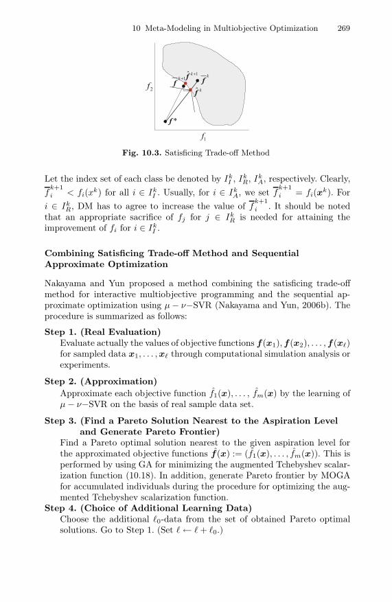
Next, we consider the following problem (Ex-1):

minimize f1 := x1 + x2

f2 := 20 cos(15x1) + (x1 − 4)4 + 100 sin(x1x2)subject to 0 � x1, x2 � 3.

The true function of each objective function f1 and f2 in the problem (Ex-1)are shown in Fig. 10.4.

0 1 2 30

0.5

1

1.5

2

2.5

3

x1

x2

(a) f1

0 1 2 30

0.5

1

1.5

2

2.5

3

x1

x2

(b) f2

Fig. 10.4. The true contours to the problem

In our simulation, the ideal point and the aspiration level is respectively givenby


0 1 2 30

0.5

1

1.5

2

2.5

3

x1

x2

(a) contour of f1

0 1 2 30

0.5

1

1.5

2

2.5

3

x1

x2

(b) contour of f2

0 1 2 3 4

−100

−50

0

50

100

150

200

250

300

f1

f 2

ideal point

aspiration level

(c) population at the final generation

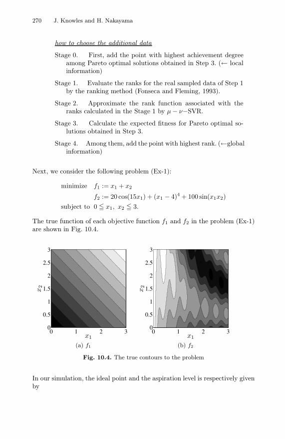
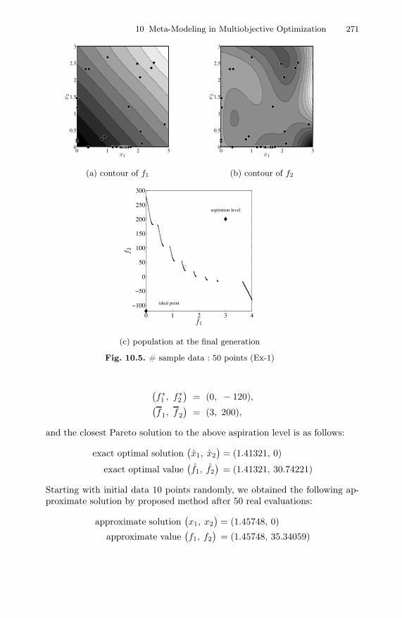
Fig. 10.5. # sample data : 50 points (Ex-1)

(f∗1 , f∗

2

)= (0, − 120),

(f1, f2

)= (3, 200),

and the closest Pareto solution to the above aspiration level is as follows:

exact optimal solution(x1, x2

)= (1.41321, 0)

exact optimal value(f1, f2

)= (1.41321, 30.74221)

Starting with initial data 10 points randomly, we obtained the following ap-proximate solution by proposed method after 50 real evaluations:

approximate solution(x1, x2

)= (1.45748, 0)

approximate value(f1, f2

)= (1.45748, 35.34059)


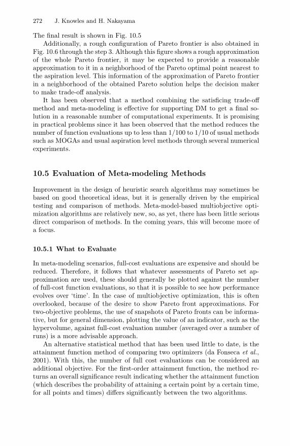
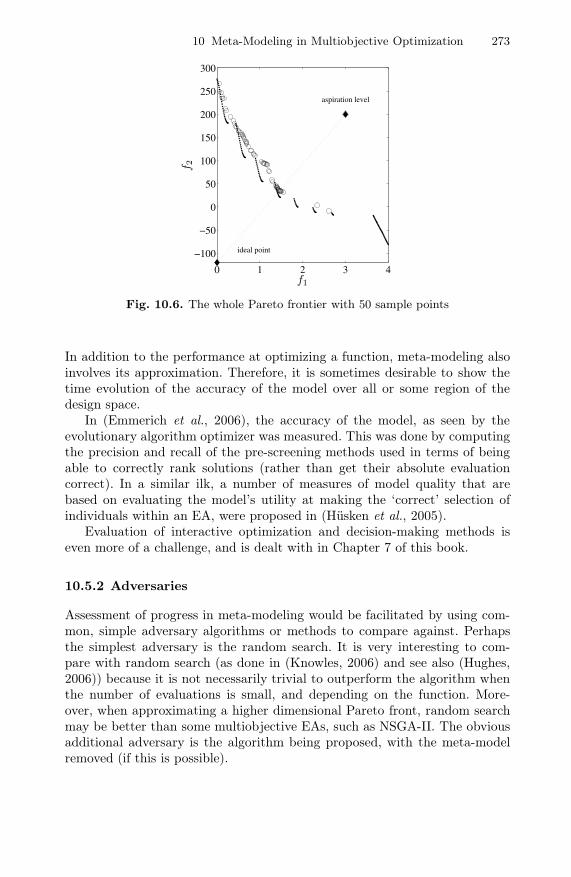
The final result is shown in Fig. 10.5Additionally, a rough configuration of Pareto frontier is also obtained in

Fig. 10.6 through the step 3. Although this figure shows a rough approximationof the whole Pareto frontier, it may be expected to provide a reasonableapproximation to it in a neighborhood of the Pareto optimal point nearest tothe aspiration level. This information of the approximation of Pareto frontierin a neighborhood of the obtained Pareto solution helps the decision makerto make trade-off analysis.

It has been observed that a method combining the satisficing trade-offmethod and meta-modeling is effective for supporting DM to get a final so-lution in a reasonable number of computational experiments. It is promisingin practical problems since it has been observed that the method reduces thenumber of function evaluations up to less than 1/100 to 1/10 of usual methodssuch as MOGAs and usual aspiration level methods through several numericalexperiments.

10.5 Evaluation of Meta-modeling Methods

Improvement in the design of heuristic search algorithms may sometimes bebased on good theoretical ideas, but it is generally driven by the empiricaltesting and comparison of methods. Meta-model-based multiobjective opti-mization algorithms are relatively new, so, as yet, there has been little seriousdirect comparison of methods. In the coming years, this will become more ofa focus.

10.5.1 What to Evaluate

In meta-modeling scenarios, full-cost evaluations are expensive and should bereduced. Therefore, it follows that whatever assessments of Pareto set ap-proximation are used, these should generally be plotted against the numberof full-cost function evaluations, so that it is possible to see how performanceevolves over ‘time’. In the case of multiobjective optimization, this is oftenoverlooked, because of the desire to show Pareto front approximations. Fortwo-objective problems, the use of snapshots of Pareto fronts can be informa-tive, but for general dimension, plotting the value of an indicator, such as thehypervolume, against full-cost evaluation number (averaged over a number ofruns) is a more advisable approach.

An alternative statistical method that has been used little to date, is theattainment function method of comparing two optimizers (da Fonseca et al.,2001). With this, the number of full cost evaluations can be considered anadditional objective. For the first-order attainment function, the method re-turns an overall significance result indicating whether the attainment function(which describes the probability of attaining a certain point by a certain time,for all points and times) differs significantly between the two algorithms.


0 1 2 3 4

−100

−50

0

50

100

150

200

250

300

f1

f 2

ideal point

aspiration level

Fig. 10.6. The whole Pareto frontier with 50 sample points

In addition to the performance at optimizing a function, meta-modeling alsoinvolves its approximation. Therefore, it is sometimes desirable to show thetime evolution of the accuracy of the model over all or some region of thedesign space.

In (Emmerich et al., 2006), the accuracy of the model, as seen by theevolutionary algorithm optimizer was measured. This was done by computingthe precision and recall of the pre-screening methods used in terms of beingable to correctly rank solutions (rather than get their absolute evaluationcorrect). In a similar ilk, a number of measures of model quality that arebased on evaluating the model’s utility at making the ‘correct’ selection ofindividuals within an EA, were proposed in (Hüsken et al., 2005).

Evaluation of interactive optimization and decision-making methods iseven more of a challenge, and is dealt with in Chapter 7 of this book.

10.5.2 Adversaries

Assessment of progress in meta-modeling would be facilitated by using com-mon, simple adversary algorithms or methods to compare against. Perhapsthe simplest adversary is the random search. It is very interesting to com-pare with random search (as done in (Knowles, 2006) and see also (Hughes,2006)) because it is not necessarily trivial to outperform the algorithm whenthe number of evaluations is small, and depending on the function. More-over, when approximating a higher dimensional Pareto front, random searchmay be better than some multiobjective EAs, such as NSGA-II. The obviousadditional adversary is the algorithm being proposed, with the meta-modelremoved (if this is possible).


10.6 Real Applications

10.6.1 Closed-Loop Mass-Spectrometer Optimization

Mass spectrometers are analytical instruments for determining the chemicalcompounds present in a sample. Typically, they are used for testing a hy-pothesis as to whether a particular compound is present or not. When usedin this way, the instrument can be configured according to standard princi-ples and settings provided by the instrument manufacturer. However, modernbiological applications aim at using mass-spectrometry to mine data with-out a hypothesis, i.e. to measure/detect simultaneously the hundreds of com-pounds contained in complex biological samples. For such applications, themass spectrometer will not perform well in a standard configuration, so itmust be optimized.

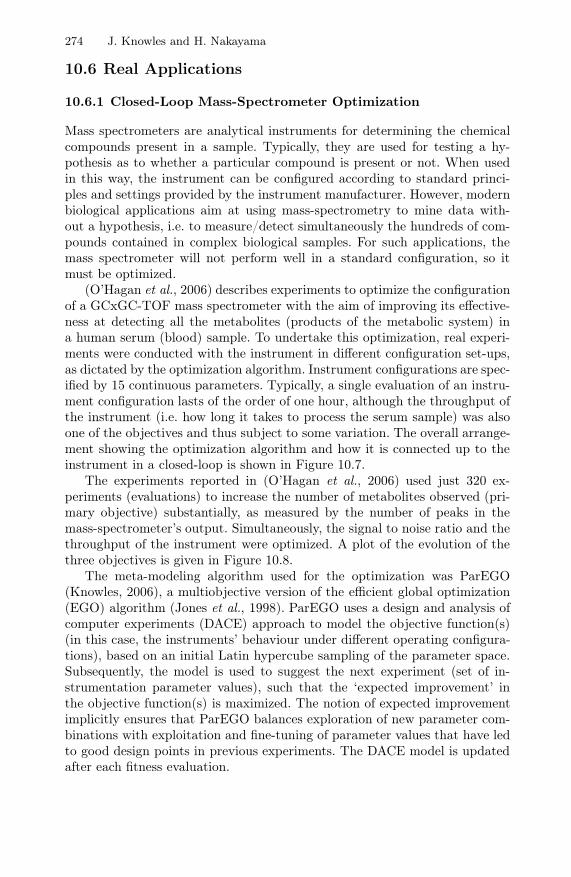
(O’Hagan et al., 2006) describes experiments to optimize the configurationof a GCxGC-TOF mass spectrometer with the aim of improving its effective-ness at detecting all the metabolites (products of the metabolic system) ina human serum (blood) sample. To undertake this optimization, real experi-ments were conducted with the instrument in different configuration set-ups,as dictated by the optimization algorithm. Instrument configurations are spec-ified by 15 continuous parameters. Typically, a single evaluation of an instru-ment configuration lasts of the order of one hour, although the throughput ofthe instrument (i.e. how long it takes to process the serum sample) was alsoone of the objectives and thus subject to some variation. The overall arrange-ment showing the optimization algorithm and how it is connected up to theinstrument in a closed-loop is shown in Figure 10.7.

The experiments reported in (O’Hagan et al., 2006) used just 320 ex-periments (evaluations) to increase the number of metabolites observed (pri-mary objective) substantially, as measured by the number of peaks in themass-spectrometer’s output. Simultaneously, the signal to noise ratio and thethroughput of the instrument were optimized. A plot of the evolution of thethree objectives is given in Figure 10.8.

The meta-modeling algorithm used for the optimization was ParEGO(Knowles, 2006), a multiobjective version of the efficient global optimization(EGO) algorithm (Jones et al., 1998). ParEGO uses a design and analysis ofcomputer experiments (DACE) approach to model the objective function(s)(in this case, the instruments’ behaviour under different operating configura-tions), based on an initial Latin hypercube sampling of the parameter space.Subsequently, the model is used to suggest the next experiment (set of in-strumentation parameter values), such that the ‘expected improvement’ inthe objective function(s) is maximized. The notion of expected improvementimplicitly ensures that ParEGO balances exploration of new parameter com-binations with exploitation and fine-tuning of parameter values that have ledto good design points in previous experiments. The DACE model is updatedafter each fitness evaluation.


Generate Gaussian Processmodel of the scalarized fitness based

on matrix M

Choose a scalarizing weight vector

improvement in the scalarized fitness

Search for a configuration x

Expensive evaluation step

Do an experiment with theGCxGC mass spectrometer

configured according to x

yMeasure the three objectives and store in the matrix Mx,y

x

Main loop

Initialization

based on a latinhypercube design

sample configurationsDefine initial k

that maximizes the expected

Fig. 10.7. Closed-loop optimization of mass spectrometer parameters using theParEGO algorithm

10.6.2 Application to Reinforcement of Cable-Stayed Bridges

After the big earthquake in Kobe in 1995, many in-service structures wererequired to improve their anti-seismic property by law regulation in Japan.However, it is very difficult for large and/or complicated bridges, such assuspension bridges, cable-stayed bridges, arch bridges and so on, to be rein-forced because of impractical executing methods and complicated dynamicresponses. Recently, many kinds of anti-seismic device have been developed(Honda et al., 2004). It is practical in the bridge to be installed a numberof small devices taking into account of strength and/or space, and to obtainthe most reasonable arrangement and capacity of the devices by using op-timization technique. In this problem, the form of objective function is notgiven explicitly in terms of design variables, but the value of the function isobtained by seismic response analysis. Since this analysis needs much cost andlong time, it is strongly desirable to make the number of analyses as few aspossible. To this end, radial basis function networks (RBFN) are employedin predicting the form of objective function, and genetic algorithms (GA) insearching the optimal value of the predicted objective function (Nakayamaet al., 2006).

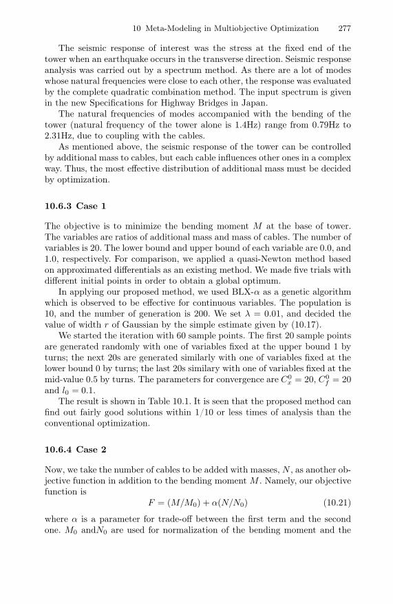
The proposed method was appplied to a problem of anti-seismic improve-ment of a cable-stayed bridge which typifies the difficulty of reinforcement ofin-service structure. In this investigation, we determine an efficient arrange-ment and amount of additional mass for cables to reduce the seismic responseof the tower of a cable-stayed bridge (Fig. 10.9).


10

15

20

20

40

60

80

1000

2000

3000

4000

Signal:Noise RatioRuntime /mins

#Peaks

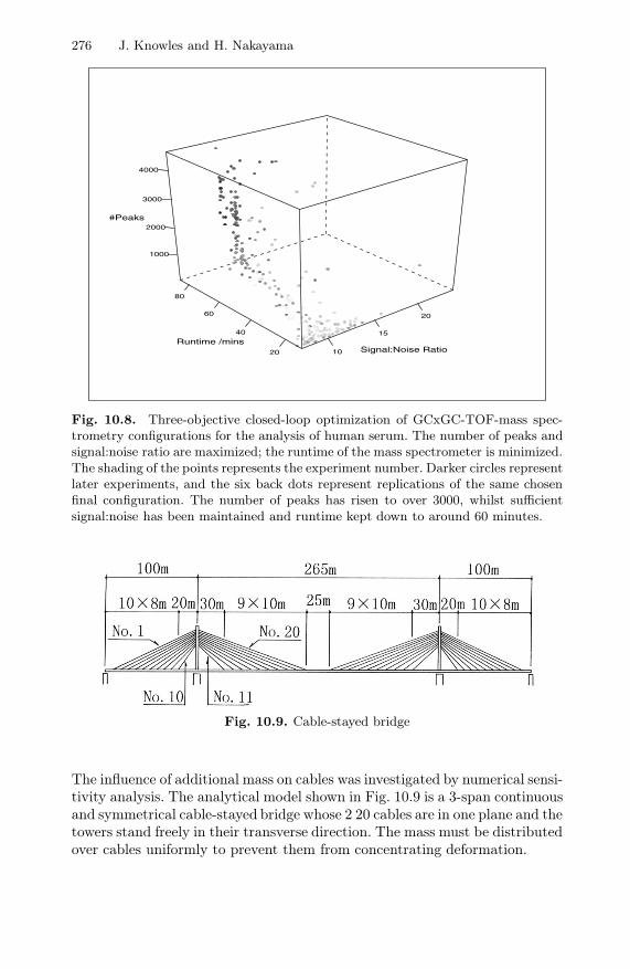
Fig. 10.8. Three-objective closed-loop optimization of GCxGC-TOF-mass spec-trometry configurations for the analysis of human serum. The number of peaks andsignal:noise ratio are maximized; the runtime of the mass spectrometer is minimized.The shading of the points represents the experiment number. Darker circles representlater experiments, and the six back dots represent replications of the same chosenfinal configuration. The number of peaks has risen to over 3000, whilst sufficientsignal:noise has been maintained and runtime kept down to around 60 minutes.

Fig. 10.9. Cable-stayed bridge

The influence of additional mass on cables was investigated by numerical sensi-tivity analysis. The analytical model shown in Fig. 10.9 is a 3-span continuousand symmetrical cable-stayed bridge whose 2 20 cables are in one plane and thetowers stand freely in their transverse direction. The mass must be distributedover cables uniformly to prevent them from concentrating deformation.


The seismic response of interest was the stress at the fixed end of thetower when an earthquake occurs in the transverse direction. Seismic responseanalysis was carried out by a spectrum method. As there are a lot of modeswhose natural frequencies were close to each other, the response was evaluatedby the complete quadratic combination method. The input spectrum is givenin the new Specifications for Highway Bridges in Japan.

The natural frequencies of modes accompanied with the bending of thetower (natural frequency of the tower alone is 1.4Hz) range from 0.79Hz to2.31Hz, due to coupling with the cables.

As mentioned above, the seismic response of the tower can be controlledby additional mass to cables, but each cable influences other ones in a complexway. Thus, the most effective distribution of additional mass must be decidedby optimization.

10.6.3 Case 1

The objective is to minimize the bending moment M at the base of tower.The variables are ratios of additional mass and mass of cables. The number ofvariables is 20. The lower bound and upper bound of each variable are 0.0, and1.0, respectively. For comparison, we applied a quasi-Newton method basedon approximated differentials as an existing method. We made five trials withdifferent initial points in order to obtain a global optimum.

In applying our proposed method, we used BLX-α as a genetic algorithmwhich is observed to be effective for continuous variables. The population is10, and the number of generation is 200. We set λ = 0.01, and decided thevalue of width r of Gaussian by the simple estimate given by (10.17).

We started the iteration with 60 sample points. The first 20 sample pointsare generated randomly with one of variables fixed at the upper bound 1 byturns; the next 20s are generated similarly with one of variables fixed at thelower bound 0 by turns; the last 20s similary with one of variables fixed at themid-value 0.5 by turns. The parameters for convergence are C0

x = 20, C0f = 20

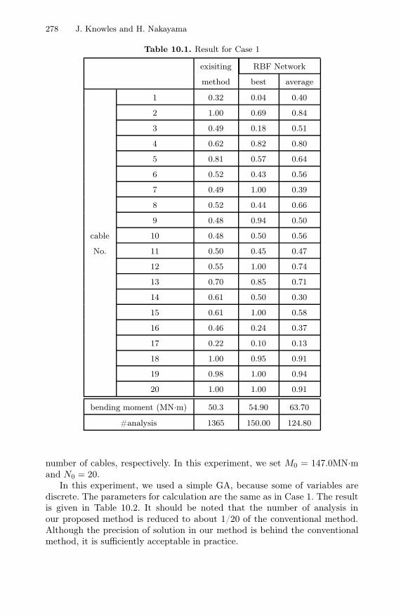
and l0 = 0.1.The result is shown in Table 10.1. It is seen that the proposed method can

find out fairly good solutions within 1/10 or less times of analysis than theconventional optimization.

10.6.4 Case 2

Now, we take the number of cables to be added with masses, N , as another ob-jective function in addition to the bending moment M . Namely, our objectivefunction is

F = (M/M0) + α(N/N0) (10.21)

where α is a parameter for trade-off between the first term and the secondone. M0 andN0 are used for normalization of the bending moment and the


Table 10.1. Result for Case 1

exisiting RBF Network

method best average

1 0.32 0.04 0.40

2 1.00 0.69 0.84

3 0.49 0.18 0.51

4 0.62 0.82 0.80

5 0.81 0.57 0.64

6 0.52 0.43 0.56

7 0.49 1.00 0.39

8 0.52 0.44 0.66

9 0.48 0.94 0.50

cable 10 0.48 0.50 0.56

No. 11 0.50 0.45 0.47

12 0.55 1.00 0.74

13 0.70 0.85 0.71

14 0.61 0.50 0.30

15 0.61 1.00 0.58

16 0.46 0.24 0.37

17 0.22 0.10 0.13

18 1.00 0.95 0.91

19 0.98 1.00 0.94

20 1.00 1.00 0.91

bending moment (MN·m) 50.3 54.90 63.70

#analysis 1365 150.00 124.80

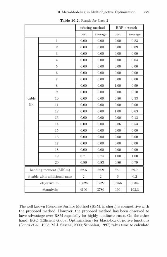
number of cables, respectively. In this experiment, we set M0 = 147.0MN·mand N0 = 20.

In this experiment, we used a simple GA, because some of variables arediscrete. The parameters for calculation are the same as in Case 1. The resultis given in Table 10.2. It should be noted that the number of analysis inour proposed method is reduced to about 1/20 of the conventional method.Although the precision of solution in our method is behind the conventionalmethod, it is sufficiently acceptable in practice.


Table 10.2. Result for Case 2

existing method RBF network

best average best average

1 0.00 0.00 0.00 0.83

2 0.00 0.00 0.00 0.09

3 0.00 0.00 0.00 0.00

4 0.00 0.00 0.00 0.04

5 0.00 0.00 0.00 0.00

6 0.00 0.00 0.00 0.00

7 0.00 0.00 0.00 0.00

8 0.00 0.00 1.00 0.99

9 0.00 0.00 0.00 0.10

cable 10 0.00 0.00 0.86 0.53

No. 11 0.00 0.00 0.00 0.00

12 0.00 0.00 1.00 0.63

13 0.00 0.00 0.00 0.13

14 0.00 0.00 0.86 0.53

15 0.00 0.00 0.00 0.00

16 0.00 0.00 0.00 0.00

17 0.00 0.00 0.00 0.00

18 0.00 0.00 0.00 0.00

19 0.71 0.74 1.00 1.00

20 0.86 0.83 0.86 0.79

bending moment (MN·m) 62.6 62.8 67.1 69.7

#cable with additional mass 2 2 6 6.2

objective fn. 0.526 0.527 0.756 0.784

#analysis 4100 3780 199 193.3

The well known Response Surface Method (RSM, in short) is competitive withthe proposed method. However, the proposed method has been observed tohave advantage over RSM especially for highly nonlinear cases. On the otherhand, EGO (Efficient Global Optimization) for black-box objective functions(Jones et al., 1998; M.J. Sasena, 2000; Schonlau, 1997) takes time to calculate


the expected improvement, while it is rather simple and easy to add twokinds of additional samples for global information and local information forapproximation (Nakayama et al., 2002, 2003).

10.7 Concluding Remarks

The increasing desire to apply optimization methods in expensive domainsis driving forward research in meta-modeling. Up to now, meta-modeling hasbeen applied mainly in continuous, low dimensional design variable spaces,and methods from design of experiments and response surfaces have beenused. High-dimensional discrete spaces may also arise in applications involvingexpensive evaluations and this will motivate research into meta-modeling ofthese domains too. Research in meta-modeling for multiobjective optimizationis relatively young and there is still much to do. So far, there are few standardsfor comparisons of methods, and little is yet known about the relative perfor-mance of different approaches. The state of the art research surveyed in thischapter is beginning to grapple with the issues of incremental learning andthe trade-off between exploitation and exploration within meta-modeling. Inthe future, scalability of methods in variable dimension and objective spacedimension will become important, as will methods capable of dealing withnoise or uncertainty. Interactive meta-modeling is also likely to be investi-gated more thoroughly, as the number of evaluations can be further reducedby these approaches.

References

Anderson, V.L., McLean, R.A.: Design of Experiments: A Realistic Approach. Mar-cel Dekker, New York (1974)

Atkeson, C.G., Moore, A.W., Schaal, S.: Locally weighted learning for control. Ar-tificial Intelligence Review 11(1), 75–113 (1997)

Breiman, L.: Classification and Regression Trees. Chapman and Hall, Boca Raton(1984)

Brown, G., Wyatt, J.L., Tiňo, P.: Managing diversity in regression ensembles. TheJournal of Machine Learning Research 6, 1621–1650 (2005)

Schölkopf, B., Smola, A.J.: Learning with Kernels: Support Vector Machines, Reg-ularization, Optimization, and Beyond. MIT Press, Cambridge (2002)

Cauwenberghs, G., Poggio, T.: Incremental and decremental support vector machinelearning. Advances in Neural Information Processing Systems 13, 409–415 (2001)

Chafekar, D., Shi, L., Rasheed, K., Xuan, J.: Multiobjective ga optimization usingreduced models. IEEE Transactions on Systems, Man and Cybernetics, Part C:Applications and Reviews 35(2), 261–265 (2005)

Chapelle, O., Vapnik, V., Weston, J.: Transductive inference for estimating values offunctions. Advances in Neural Information Processing Systems 12, 421–427 (1999)

Cohn, D.A., Ghahramani, Z., Jordan, M.I.: Active learning with statistical models.Journal of Artificial Intelligence Research 4, 129–145 (1996)


Corne, D.W., Oates, M.J., Kell, D.B.: On fitness distributions and expected fitnessgain of mutation rates in parallel evolutionary algorithms. In: Guervós, J.J.M.,Adamidis, P.A., Beyer, H.-G., Fernández-Villacañas, J.-L., Schwefel, H.-P. (eds.)PPSN 2002. LNCS, vol. 2439, pp. 132–141. Springer, Heidelberg (2002)

Cortes, C., Vapnik, V.: Support vector networks. Machine Learning 20, 273–297(1995)

Cristianini, N., Shawe-Tylor, J.: An Introduction to Support Vector Machines andOther Kernel-based Learning Methods. Cambridge University Press, Cambridge(2000)

Grunert da Fonseca, V., Fonseca, C.M., Hall, A.O.: Inferential Performance As-sessment of Stochastic Optimisers and the Attainment Function. In: Zitzler, E.,Deb, K., Thiele, L., Coello Coello, C.A., Corne, D.W. (eds.) EMO 2001. LNCS,vol. 1993, pp. 213–225. Springer, Heidelberg (2001)

Emmerich, M.T.M., Beume, N., Naujoks, B.: An EMO algorithm using the hyper-volume measure as selection criterion. In: Coello Coello, C.A., Hernández Aguirre,A., Zitzler, E. (eds.) EMO 2005. LNCS, vol. 3410, pp. 62–76. Springer, Heidelberg(2005)

Emmerich, M., Giannakoglou, K., Naujoks, B.: Single-and Multi-objective Evolu-tionary Optimization Assisted by Gaussian Random Field Metamodels. IEEETransactions on Evolutionary Computation 10(4), 421–439 (2006)

English, T.M.: Optimization is easy and learning is hard in the typical function. In:Proceedings of the 2000 Congress on Evolutionary Computation (CEC00), pp.924–931. IEEE Computer Society Press, Piscataway (2000)

Erenguc, S.S., Koehler, G.J.: Survey of mathematical programming models and ex-perimental results for linear discriminant analysis. Managerial and Decision Eco-nomics 11, 215–225 (1990)

Eyheramendy, S., Lewis, D., Madigan, D.: On the naive Bayes model for text cate-gorization. In: Proceedings Artificial Intelligence & Statistics 2003 (2003)

Fieldsend, J.E., Everson, R.M.: Multi-objective Optimisation in the Presence of Un-certainty. In: 2005 IEEE Congress on Evolutionary Computation (CEC’2005),Edinburgh, Scotland, September 2005, vol. 1, pp. 243–250. IEEE Computer So-ciety Press, Los Alamitos (2005)

Fonseca, C.M., Fleming, P.J.: Genetic algorithms for multi-objective optimization:Formulation, discussion and generalization. In: Proceedings of the Fifth Interna-tional Conference on Genetic Algorithms, pp. 416–426 (1993)

Freed, N., Glover, F.: Simple but powerful goal programming models for discriminantproblems. European J. of Operational Research 7, 44–60 (1981)

Gaspar-Cunha, A., Vieira, A.: A multi-objective evolutionary algorithm using neuralnetworks to approximate fitness evaluations. International Journal of Computers,Systems, and Signals (2004)

Hamza, K., Saitou, K.: Vehicle crashworthiness design via a surrogate model en-semble and a co-evolutionary genetic algorithm. In: Proc. of IDETC/CIE 2005ASME 2005 International Design Engineering Technical Conference, California,USA (2005)

Honda, M., Morishita, K., Inoue, K., Hirai, J.: Improvement of anti-seismic capacitywith damper braces for bridges. In: Proceedings of the Seventh InternationalConference on Motion and Vibration Control (2004)


Huang, D., Allen, T.T., Notz, W.I., Zeng, N.: Global Optimization of StochasticBlack-Box Systems via Sequential Kriging Meta-Models. Journal of Global Opti-mization 34(3), 441–466 (2006)

Hughes, E.J.: Evolutionary Many-Objective Optimisation: Many Once or OneMany? In: 2005 IEEE Congress on Evolutionary Computation (CEC’2005), vol. 1,pp. 222–227. IEEE Computer Society Press, Los Alamitos (2005)

Hughes, E.J.: Multi-Objective Equivalent Random Search. In: Runarsson, T.P.,Beyer, H.-G., Burke, E.K., Merelo-Guervós, J.J., Whitley, L.D., Yao, X. (eds.)PPSN 2006. LNCS, vol. 4193, pp. 463–472. Springer, Heidelberg (2006)

Hüsken, M., Jin, Y., Sendhoff, B.: Structure optimization of neural networks forevolutionary design optimization. Soft Computing 9(1), 21–28 (2005)

Jin, Y.: A comprehensive survey of fitness approximation in evolutionary compu-tation. Soft Computing - A Fusion of Foundations, Methodologies and Applica-tions 9(1), 3–12 (2005)

Jin, Y., Sendhoff, B.: Reducing fitness evaluations using clustering techniquesand neural network ensembles. In: Deb, K., et al. (eds.) GECCO 2004. LNCS,vol. 3102, pp. 688–699. Springer, Heidelberg (2004)

Jin, Y., Olhofer, M., Sendhoff, B.: Managing approximate models in evolutionaryalgorithms design optimization. In: Proceedings of the 2001 Congress on Evolu-tionary Computation, CEC2001, pp. 592–599 (2001)

Jones, D., Schonlau, M., Welch, W.: Efficient global optimization of expensive black-box functions. Journal of Global Optimization 13, 455–492 (1998)

Joslin, D., Dragovich, J., Vo, H., Terada, J.: Opportunistic fitness evaluation ina genetic algorithm for civil engineering design optimization. In: Proceedings ofthe Congress on Evolutionary Computation (CEC 2006), pp. 2904–2911. IEEEComputer Society Press, Los Alamitos (2006)

Jourdan, L., Corne, D.W., Savic, D.A., Walters, G.A.: Preliminary Investigation ofthe ‘Learnable Evolution Model’ for Faster/Better Multiobjective Water SystemsDesign. In: Coello Coello, C.A., Hernández Aguirre, A., Zitzler, E. (eds.) EMO2005. LNCS, vol. 3410, pp. 841–855. Springer, Heidelberg (2005)

Keane, A.J.: Statistical improvement criteria for use in multiobjective design opti-mization. AIAA Journal 44(4), 879–891 (2006)

Knowles, J.: ParEGO: A hybrid algorithm with on-line landscape approximationfor expensive multiobjective optimization problems. IEEE Transactions on Evo-lutionary Computation 10(1), 50–66 (2006)

Langdon, W.B., Poli, R.: Foundations of Genetic Programming. Springer, Heidelberg(2001)

Larranaga, P., Lozano, J.A.: Estimation of Distribution Algorithms: A New Tool forEvolutionary Computation. Kluwer Academic Publishers, Dordrecht (2001)

Laumanns, M., Očenášek, J.: Bayesian optimization algorithms for multi-objectiveoptimization. In: Guervós, J.J.M., Adamidis, P.A., Beyer, H.-G., Fernández-Villacañas, J.-L., Schwefel, H.-P. (eds.) PPSN 2002. LNCS, vol. 2439, pp. 298–307.Springer, Heidelberg (2002)

Michalski, R.: Learnable Evolution Model: Evolutionary Processes Guided by Ma-chine Learning. Machine Learning 38(1), 9–40 (2000)

Sasena, M.J., Papalambros, P.Y., Goovaerts, P.: Metamodeling sample criteria in aglobal optimization framework. In: 8th AIAA/NASA/USAF/ISSMO Symposiumon Multidisciplinary Analysis and Optimization, Long Beach, AIAA-2000-4921(2000)


Myers, R.H., Montgomery, D.C.: Response Surface Methodology: Process and Prod-uct Optimization using Designed Experiments. Wiley, Chichester (1995)

Nain, P., Deb, K.: A computationally effective multi-objective search and optimiza-tion technique using coarse-to-fine grain modeling. Kangal Report 2002005 (2002)

Nakayama, H., Sawaragi, Y.: Satisficing trade-off method for multi-objective pro-gramming. In: Grauer, M., Wierzbicki, A. (eds.) Interactive Decision Analysis,pp. 113–122. Springer, Heidelberg (1984)

Nakayama, H., Yun, Y.: Generating support vector machines using multiobjectiveoptimization and goal programming. In: Jin, Y. (ed.) Multi-objective MachineLearning, pp. 173–198. Springer, Heidelberg (2006a)

Nakayama, H., Yun, Y.: Support vector regression based on goal programming andmulti-objective programming. IEEE World Congress on Computational Intelli-gence, CD-ROM, Paper ID: 1536 (2006b)

Nakayama, H., Arakawa, M., Sasaki, R.: Simulation based optimization for unknownobjective functions. Optimization and Engineering 3, 201–214 (2002)

Nakayama, H., Arakawa, M., Washino, K.: Optimization for black-box objectivefunctions. In: Tseveendorj, I., Pardalos, P.M., Enkhbat, R. (eds.) Optimizationand Optimal Control, pp. 185–210. World Scientific, Singapore (2003)

Nakayama, H., Inoue, K., Yoshimori, Y.: Approximate optimization using compu-tational intelligence and its application to reinforcement of cable-stayed bridges.In: Zha, X.F., Howlett, R.J. (eds.) Integrated Intelligent Systems for EngineeringDesign, pp. 289–304. IOS Press, Amsterdam (2006)

O’Hagan, S., Dunn, W.B., Knowles, J.D., Broadhurst, D., Williams, R., Ashworth,J.J., Cameron, M., Kell, D.B.: Closed-Loop, Multiobjective Optimization of Two-Dimensional Gas Chromatography/Mass Spectrometry for Serum Metabolomics.Analytical Chemistry 79(2), 464–476 (2006)

Orr, M.: Introduction to radial basis function networks. Centre for Cognitive Science,University of Edinburgh (1996), http://www.cns.ed.ac.uk/people/mark.html

Ray, T., Smith, W.: Surrogate assisted evolutionary algorithm for multiobjective op-timization. In: 47th AIAA/ASME/ASCE/AHS/ASC Structures, Structural Dy-namics, and Materials Conference, pp. 1–8 (2006)

Robins, A.: Maintaining stability during new learning in neural networks. In: IEEEInternational Conference on Systems, Man, and Cybernetics, 1997, ’Computa-tional Cybernetics and Simulation’, vol. 4, pp. 3013–3018 (1997)

Schölkopf, B., Smola, A.: New support vector algorithms. Technical Report NC2-TR-1998-031, NeuroCOLT2 Technical report Series (1998)

Schonlau, M.: Computer Experiments and Global Optimization. Ph.D. thesis,Univ.of Waterloo, Ontario, Canada (1997)

Schwaighofer, A., Tresp, V.: Transductive and Inductive Methods for ApproximateGaussian Process Regression. Advances in Neural Information Processing Sys-tems 15, 953–960 (2003)

Vapnik, V.N.: Statistical Learning Theory. John Wiley & Sons, Chichester (1998)Voutchkov, I., Keane, A.J.: Multiobjective optimization using surrogates. Presented

at Adaptive Computing in Design and Manufacture (ACDM 06), Bristol, UK(2006)

Wolpert, D.H., Macready, W.G.: No free lunch theorems for optimization. IEEETransactions on Evolutionary Computation 1, 67–82 (1997)


Zitzler, E., Thiele, L., Laumanns, M., Fonseca, C.M., Grunert da Fonseca, V.: Perfor-mance Assessment of Multiobjective Optimizers: An Analysis and Review. IEEETransactions on Evolutionary Computation 7(2), 117–132 (2003)

Documents

10 Meta-Modeling in Multiobjective Optimization · PDF fileMeta-Modeling in Multiobjective Optimization ... and is also related to the Design of Experiments ... Iterative optimization