Embed Size (px)
Citation preview
1
Simple Keynesian Model
National Income DeterminationThree-Sector National Income
Model
2
Outline Three-Sector Model Tax Function T = f (Y) Consumption Function C = f (Yd) Government Expenditure Function G=f(Y) Aggregate Expenditure Function E = f(Y) Output-Expenditure Approach: Equilibri
um National Income Ye
3
Outline Factors affecting Ye Expenditure Multipliers k E
Tax Multipliers k T
Balanced-Budget Multipliers k B
Injection-Withdrawal Approach: Equilibrium National Income Ye
4
Outline Fiscal Policy (v.s. Monetary Policy) Recessionary Gap Yf - Ye Inflationary Gap Ye - Yf Financing the Government Budget Automatic Built-in Stabilizers

5
Three-Sector Model With the introduction of the
government sector (i.e. together with households C, firms I), aggregate expenditure E consists of one more component, government expenditure G.
E = C + I + G Still, the equilibrium condition is
Planned Y = Planned E

6
Three-Sector Model Consumption function is positively
related to disposable income Yd [slide 37 of 2-sector model],
C = f(Yd)C= C’C= cYdC= C’ + cYd
7
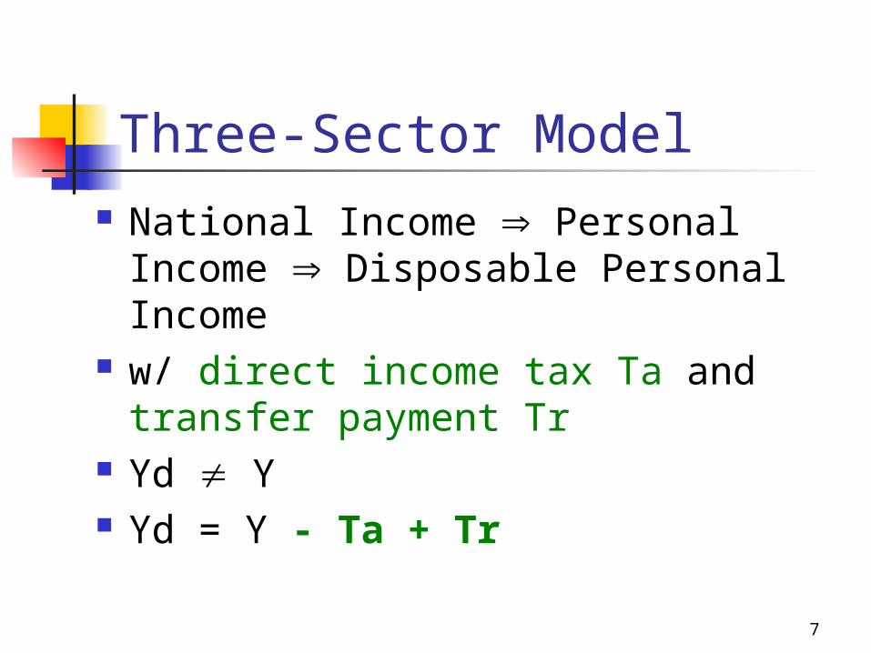
Three-Sector Model National Income Personal Income
Disposable Personal Income w/ direct income tax Ta and transfer
payment Tr Yd Y Yd = Y - Ta + Tr
8
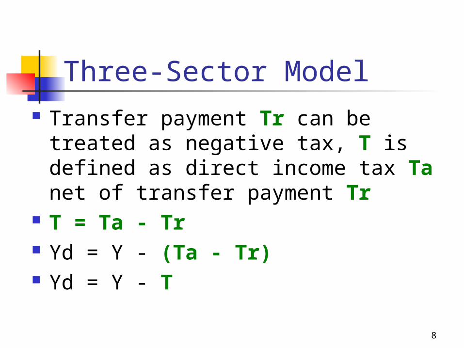
Three-Sector Model Transfer payment Tr can be treated
as negative tax, T is defined as direct income tax Ta net of transfer payment Tr
T = Ta - Tr Yd = Y - (Ta - Tr) Yd = Y - T
9
Three-Sector Model The assumptions for the 2-sector
Keynesian model are still valid for this 3-sector model [slide 24-25 of 2-sector model]
10
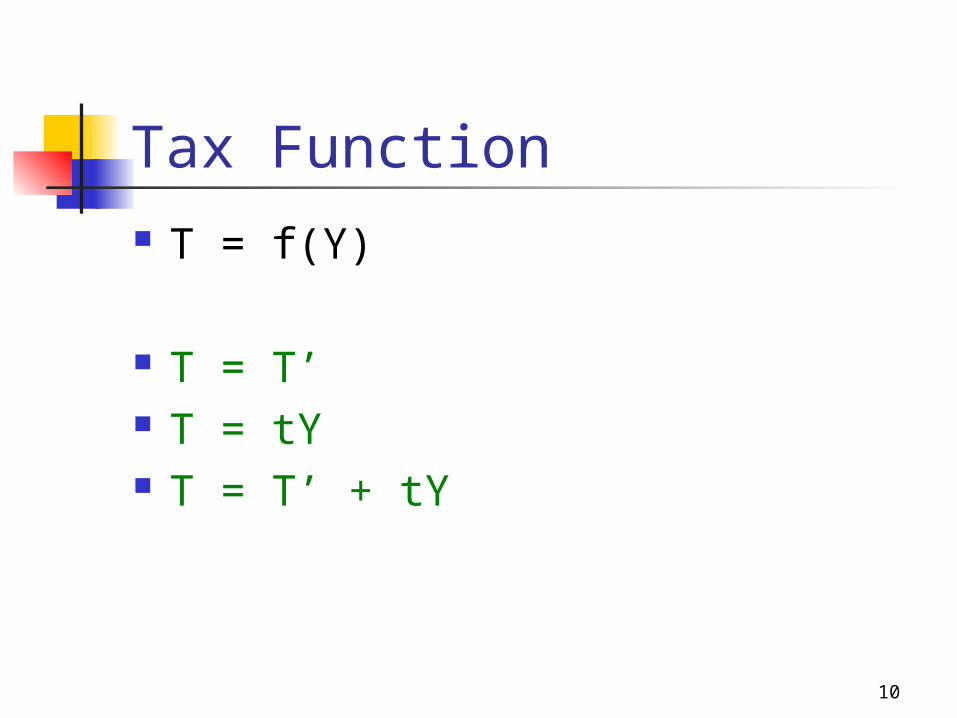
Tax Function T = f(Y)
T = T’ T = tY T = T’ + tY

11
Tax Function
T = T’
Y-intercept=T’
slope of tangent=0
T = tY
Y-intercept=0
slope of tangent=t
T = T’ +tY
Y-intercept=T’
slope of tangent=t

12
Tax Function Autonomous Tax T’
this is a lump-sum tax which is independent of income level Y
Proportional Income Tax tY marginal tax rate t is a constant
Progressive Income Tax tY marginal tax rate t increases
Regressive Income Tax tY marginal tax rate t decreases

13
Consumption Function C = f(Yd) C = C’
C = C’ C = cYd
C = c(Y - T) C = C’ + cYd
C = C’ + c(Y - T)
14
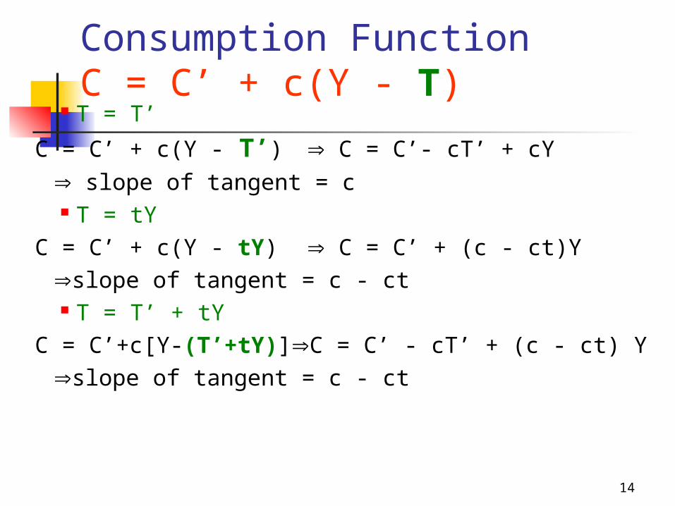
Consumption FunctionC = C’ + c(Y - T)
T = T’
C = C’ + c(Y - T’) C = C’- cT’ + cY
slope of tangent = c T = tY
C = C’ + c(Y - tY) C = C’ + (c - ct)Yslope of tangent = c - ct
T = T’ + tYC = C’+c[Y-(T’+tY)]C = C’ - cT’ + (c - ct) Y
slope of tangent = c - ct

15
Consumption FunctionC = C’ + c (Y - T’)
Y-intercept = C’ - cT’
slope of tangent = c = MPC
slope of ray APC when Y
16
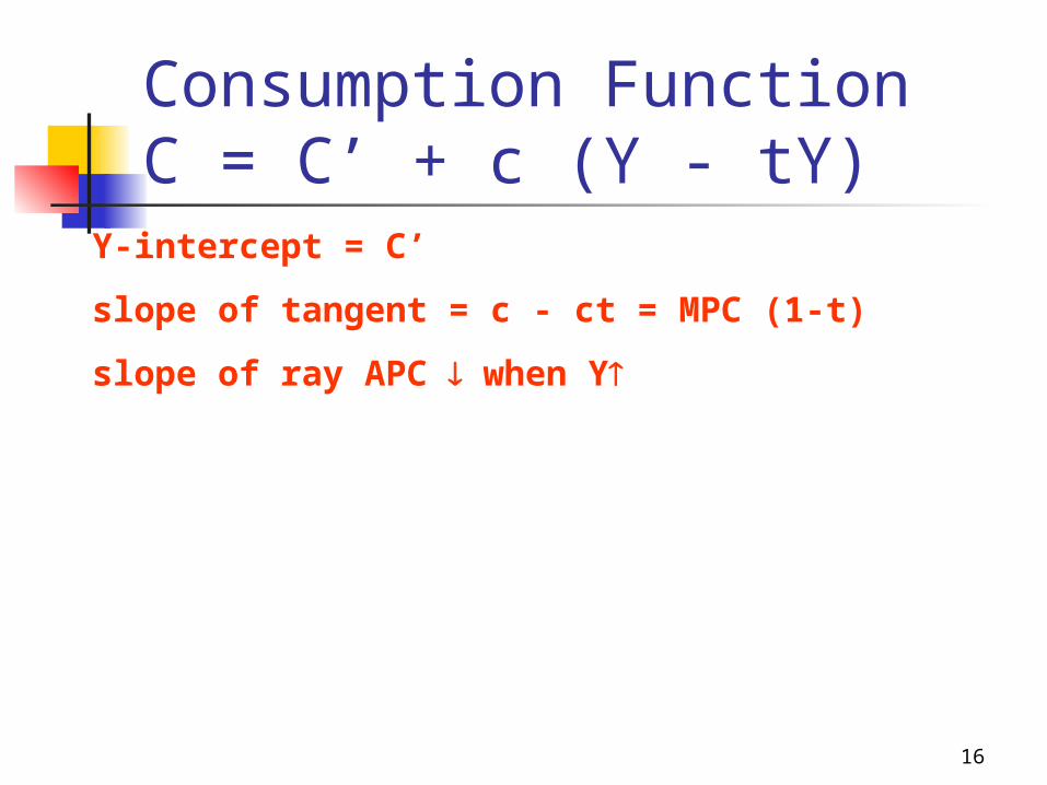
Consumption FunctionC = C’ + c (Y - tY)
Y-intercept = C’
slope of tangent = c - ct = MPC (1-t)
slope of ray APC when Y
17
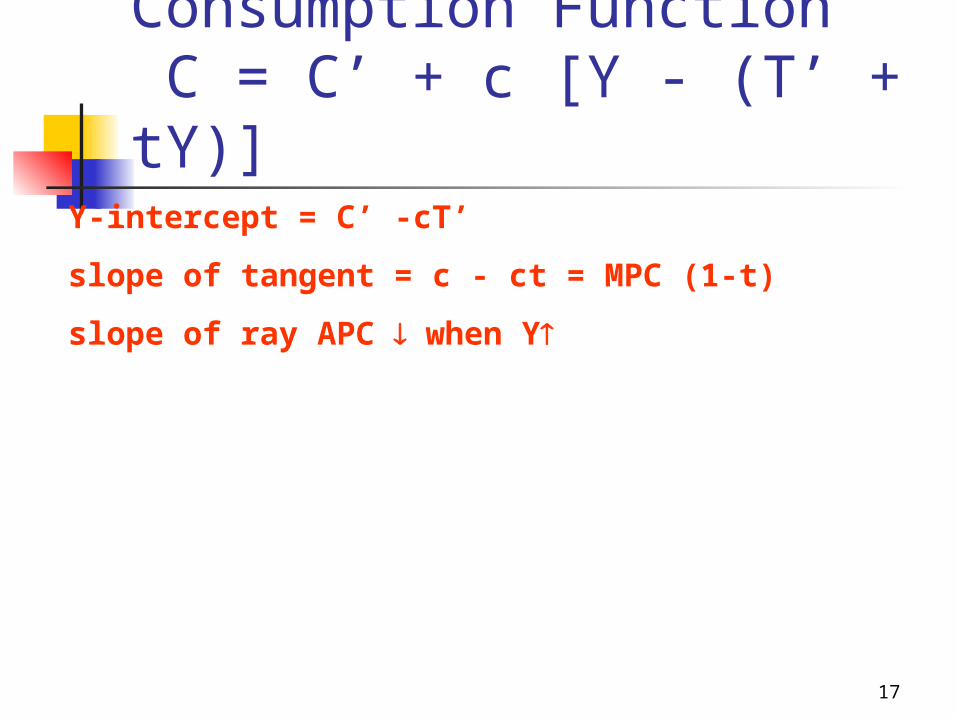
Consumption Function C = C’ + c [Y - (T’ + tY)]
Y-intercept = C’ -cT’
slope of tangent = c - ct = MPC (1-t)
slope of ray APC when Y

18
Consumption Function C = C’ - cT’ + (c - ct)Y
C’ OR T’ y-intercept C’ - cT’ C shift upward
t c(1-t) C flatter
c c(1-t) C steeper y-intercept C’ - cT’ C shift downward
19
Government Expenditure Function
G only includes the part of government expenditure spending on goods and services, i.e. transfer payments Tr are excluded.
Usually, G is assumed to be an exogenous / autonomous function
G = G’

20
Government Expenditure Function
Y-intercept = G’
slope of tangent = 0
slope of ray when Y
21
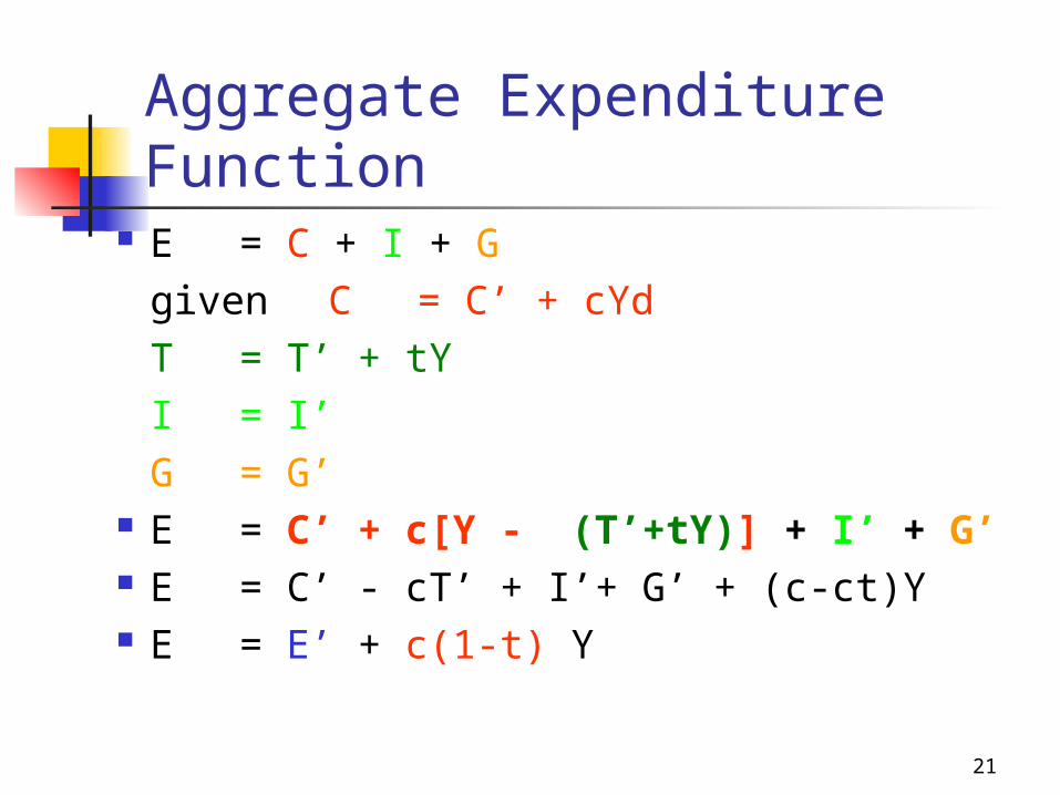
Aggregate Expenditure Function
E = C + I + Ggiven C = C’ + cYdT = T’ + tYI = I’G = G’
E = C’ + c[Y - (T’+tY)] + I’ + G’ E = C’ - cT’ + I’+ G’ + (c-ct)Y E = E’ + c(1-t) Y
22
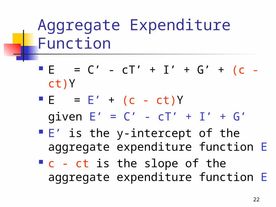
Aggregate Expenditure Function
E = C’ - cT’ + I’ + G’ + (c - ct)Y E = E’ + (c - ct)Y
given E’ = C’ - cT’ + I’ + G’ E’ is the y-intercept of the
aggregate expenditure function E c - ct is the slope of the aggregate
expenditure function E
23
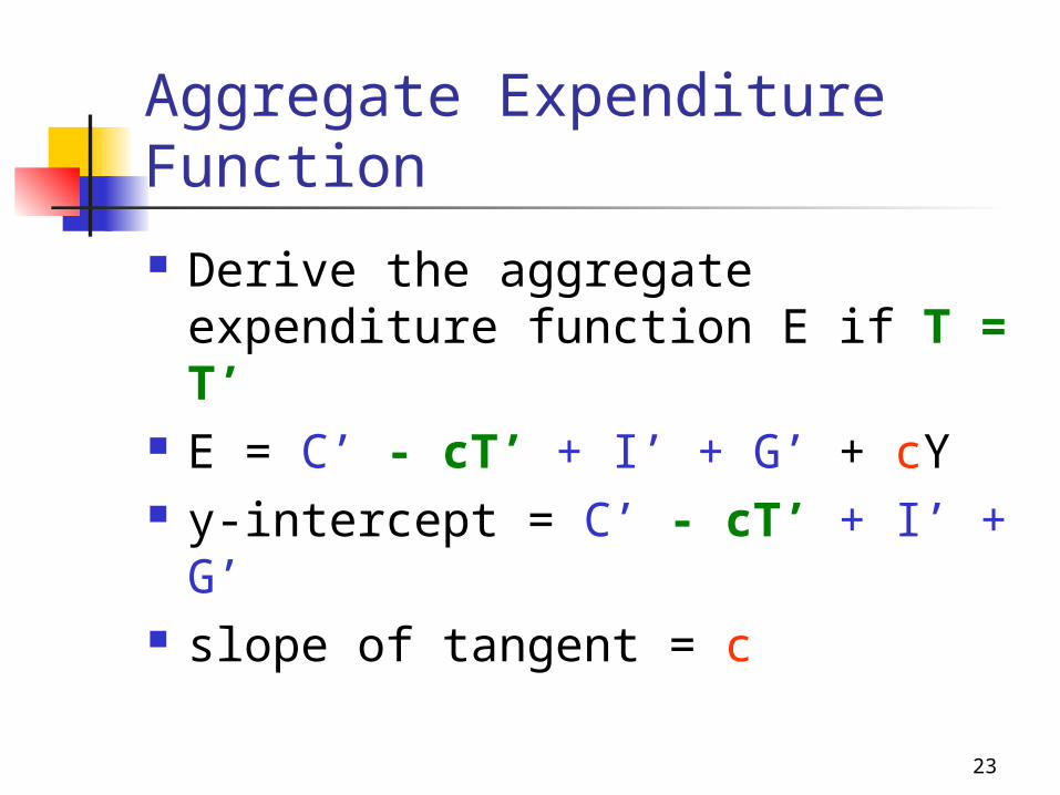
Aggregate Expenditure Function
Derive the aggregate expenditure function E if T = T’
E = C’ - cT’ + I’ + G’ + cY y-intercept = C’ - cT’ + I’ + G’ slope of tangent = c
24
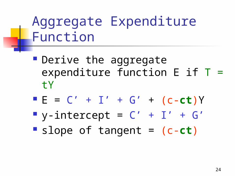
Aggregate Expenditure Function
Derive the aggregate expenditure function E if T = tY
E = C’ + I’ + G’ + (c-ct)Y y-intercept = C’ + I’ + G’ slope of tangent = (c-ct)

25
Aggregate Expenditure Function
Derive the aggregate expenditure function E if T = T’ and I = I’ + iY
E = C’ - cT’ + I’ + G’ + (c + i)Y y-intercept = C’ - cT’ + I’ + G’ slope of tangent = (c + i)
26
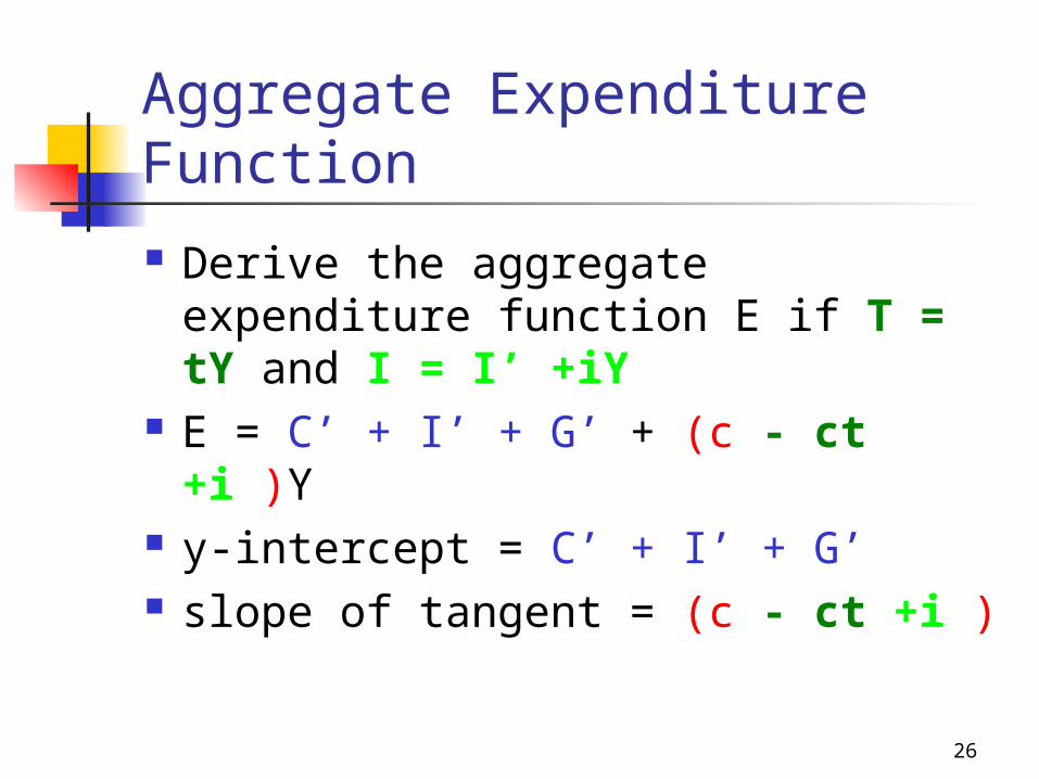
Aggregate Expenditure Function
Derive the aggregate expenditure function E if T = tY and I = I’ +iY
E = C’ + I’ + G’ + (c - ct +i )Y y-intercept = C’ + I’ + G’ slope of tangent = (c - ct +i )
27
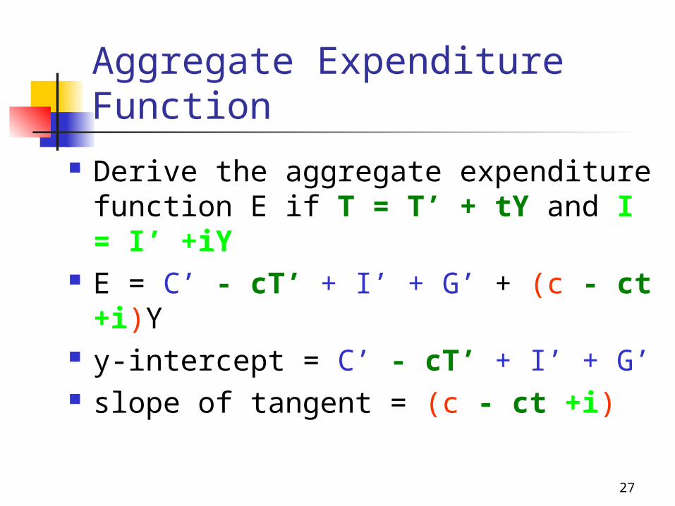
Aggregate Expenditure Function
Derive the aggregate expenditure function E if T = T’ + tY and I = I’ +iY
E = C’ - cT’ + I’ + G’ + (c - ct +i)Y y-intercept = C’ - cT’ + I’ + G’ slope of tangent = (c - ct +i)
28
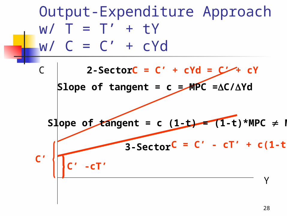
Output-Expenditure Approachw/ T = T’ + tYw/ C = C’ + cYd
Y
C C = C’ + cYd = C’ + cY
C = C’ - cT’ + c(1-t)Y
C’C’ -cT’
Slope of tangent = c = MPC =C/Yd
Slope of tangent = c (1-t) = (1-t)*MPC MPC
2-Sector
3-Sector

29
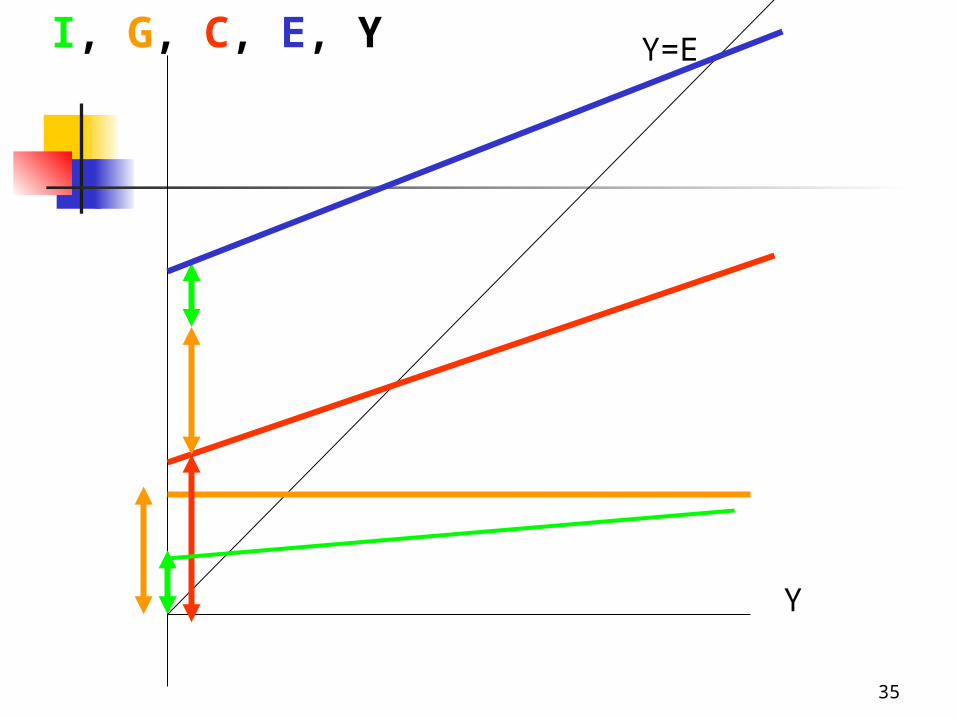
Y
I, G, C, E, Y
Planned Y = Planned E
Y=E
30
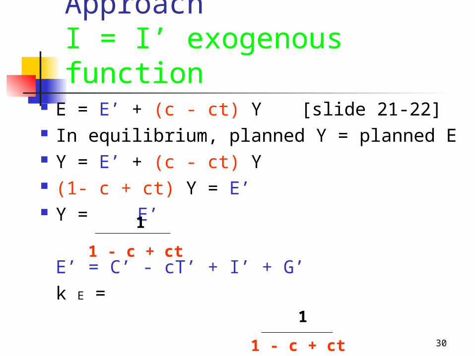
Output-Expenditure ApproachI = I’ exogenous function
E = E’ + (c - ct) Y [slide 21-22] In equilibrium, planned Y = planned E Y = E’ + (c - ct) Y (1- c + ct) Y = E’ Y = E’
E’ = C’ - cT’ + I’ + G’k E =
1
1 - c + ct
1
1 - c + ct
31
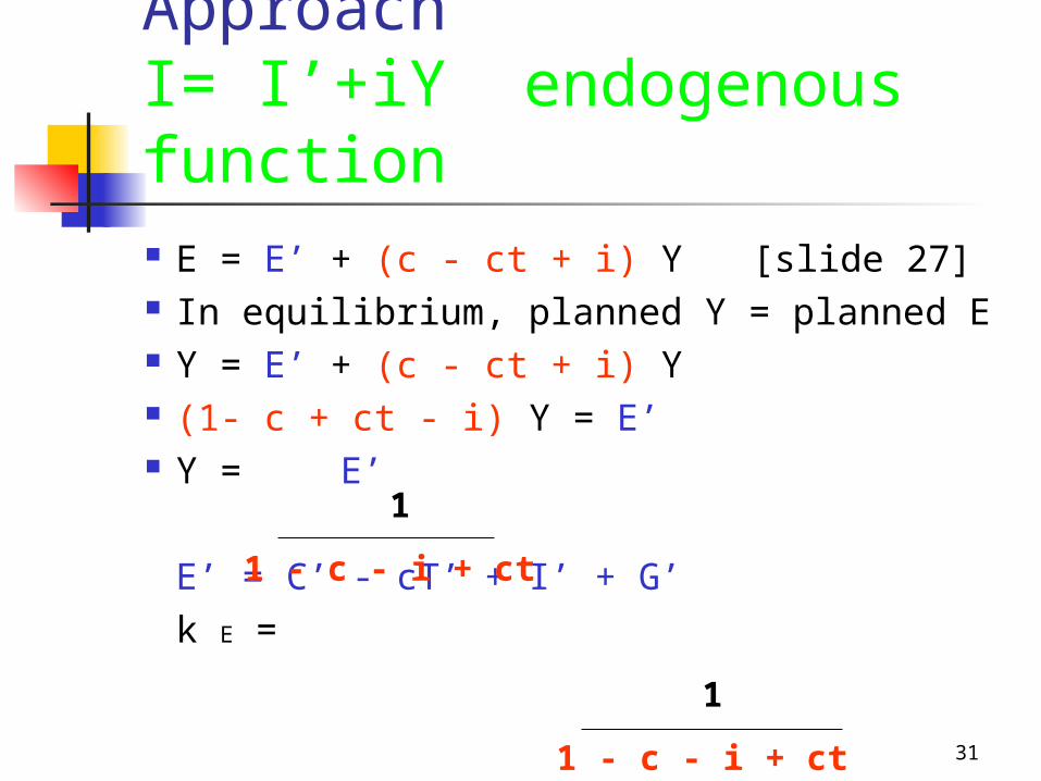
Output-Expenditure ApproachI= I’+iY endogenous function E = E’ + (c - ct + i) Y [slide 27] In equilibrium, planned Y = planned E Y = E’ + (c - ct + i) Y (1- c + ct - i) Y = E’ Y = E’
E’ = C’ - cT’ + I’ + G’k E =
1
1 - c - i + ct
1
1 - c - i + ct
32
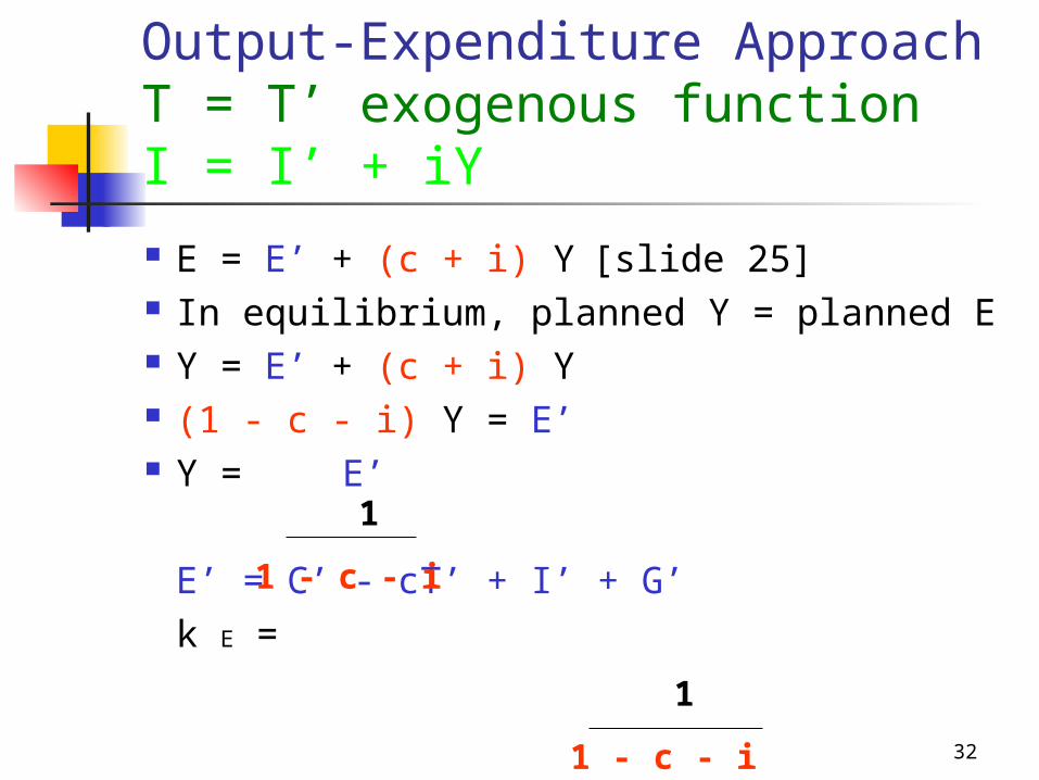
Output-Expenditure ApproachT = T’ exogenous functionI = I’ + iY
E = E’ + (c + i) Y [slide 25] In equilibrium, planned Y = planned E Y = E’ + (c + i) Y (1 - c - i) Y = E’ Y = E’
E’ = C’ - cT’ + I’ + G’k E =
1
1 - c - i
1
1 - c - i
33
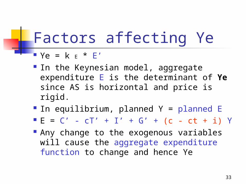
Factors affecting Ye Ye = k E * E’ In the Keynesian model, aggregate
expenditure E is the determinant of Ye since AS is horizontal and price is rigid.
In equilibrium, planned Y = planned E E = C’ - cT’ + I’ + G’ + (c - ct + i) Y Any change to the exogenous variables
will cause the aggregate expenditure function to change and hence Ye
34
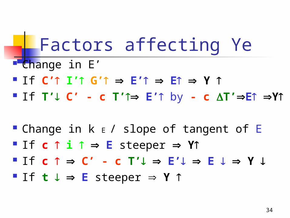
Factors affecting Ye Change in E’ If C’ I’ G’ E’ E Y If T’ C’ - c T’ E’ by - c T’E Y
Change in k E / slope of tangent of E If c i E steeper Y If c C’ - c T’ E’ E Y If t E steeper Y
35
Y
I, G, C, E, Y Y=E
36
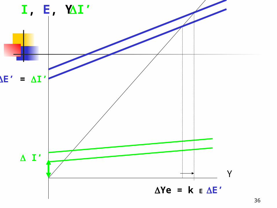
Y
I, E, Y I’
I’
E’ = I’
Ye = k E E’

37
Y
G, E, YG’

38
Y
C, E, Y C’
39
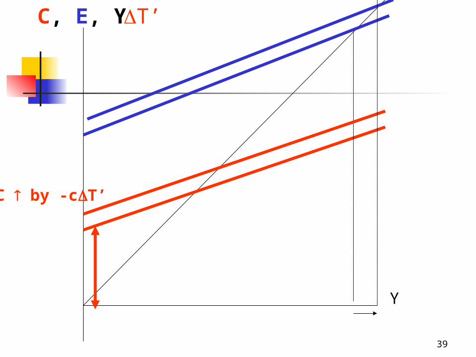
Y
C, E, Y T’
C by -cT’
40
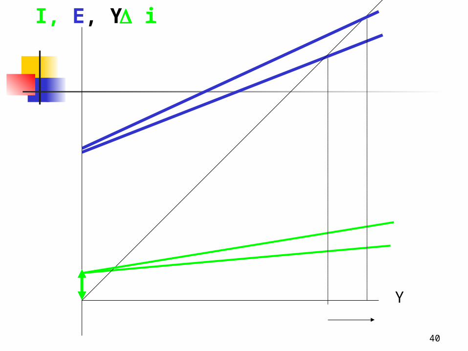
Y
I, E, Y i
41
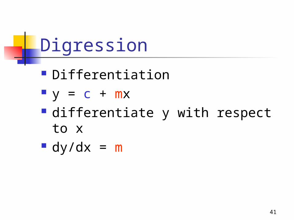
Digression Differentiation y = c + mx differentiate y with respect to x dy/dx = m
42
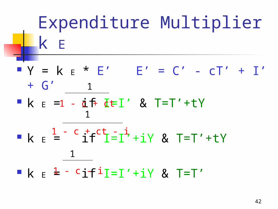
Expenditure Multiplier k E Y = k E * E’ E’ = C’ - cT’ + I’ + G’ k E = if I=I’ & T=T’+tY
k E = if I=I’+iY & T=T’+tY
k E = if I=I’+iY & T=T’
1
1 - c + ct 1
1 - c + ct - i
1
1 - c - i
43
Expenditure Multiplier k E Whenever there is a change in the
autonomous spending C’ I’ or G’ the national income Ye will change by a multiple of k E.
It actually measures the ratio of the change in national income Ye to the change in the autonomous expenditure E’
Ye/E’ = k E
44
Tax Multiplier k T
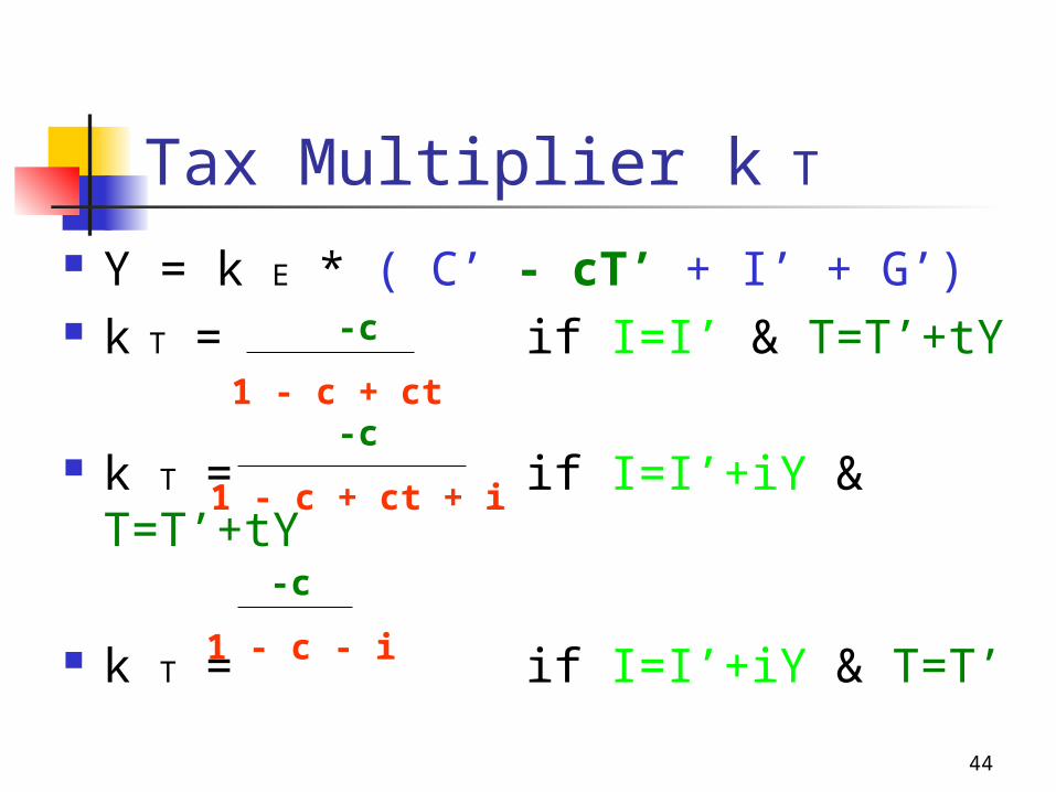
Y = k E * ( C’ - cT’ + I’ + G’) k T = if I=I’ & T=T’+tY
k T = if I=I’+iY & T=T’+tY
k T = if I=I’+iY & T=T’
-c
1 - c + ct -c
1 - c + ct + i
-c
1 - c - i
45
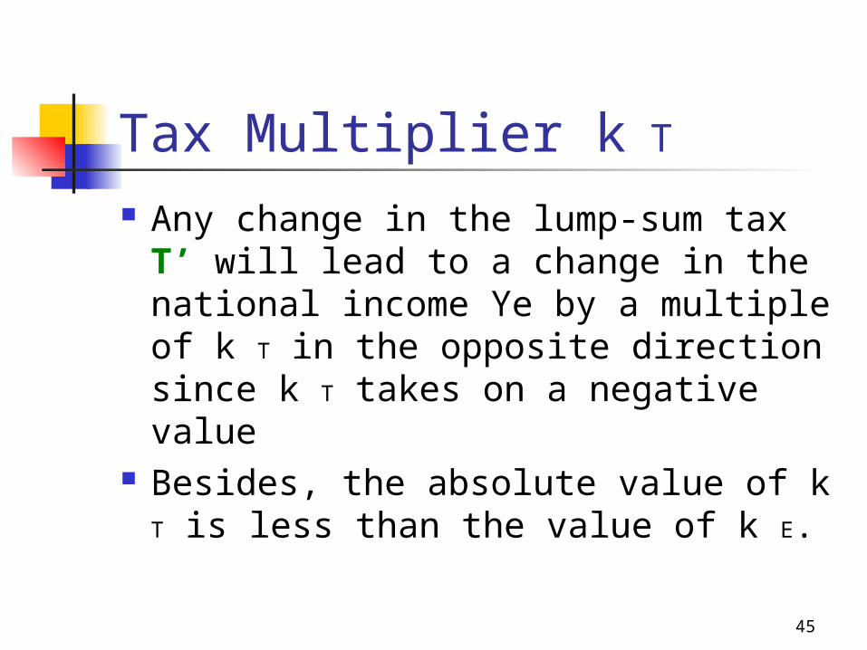
Tax Multiplier k T
Any change in the lump-sum tax T’ will lead to a change in the national income Ye by a multiple of k T in the opposite direction since k T takes on a negative value
Besides, the absolute value of k T is less than the value of k E.
46
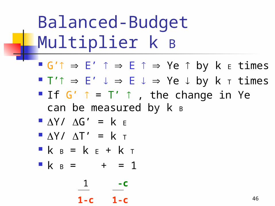
Balanced-Budget Multiplier k B G’ E’ E Ye by k E times T’ E’ E Ye by k T times If G’ = T’ , the change in Ye can be
measured by k B Y/ G’ = k E Y/ T’ = k T k B = k E + k T k B = + = 1
1
1-c
-c
1-c
47
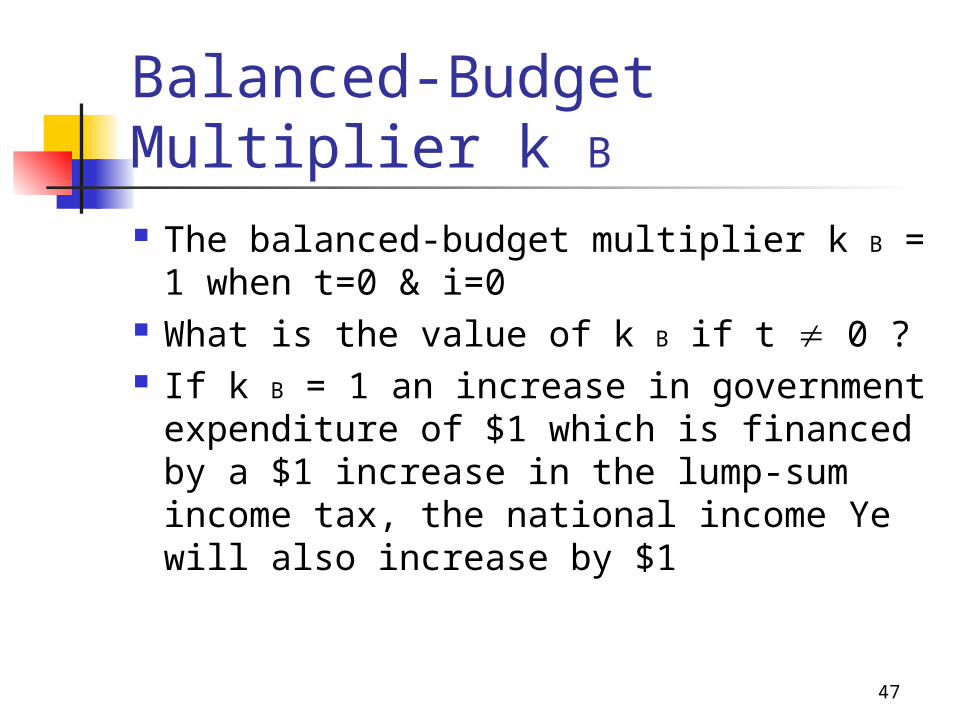
Balanced-Budget Multiplier k B The balanced-budget multiplier k B
= 1 when t=0 & i=0 What is the value of k B if t 0 ? If k B = 1 an increase in government
expenditure of $1 which is financed by a $1 increase in the lump-sum income tax, the national income Ye will also increase by $1

48
Injection-Withdrawal Approach
In a 3-sector model, national income is either consumed, saved or taxed by the government
Y = C + S + T Given E = C + I + G In equilibrium, Y = E C + S + T = C + I + G S + T = I + G
49
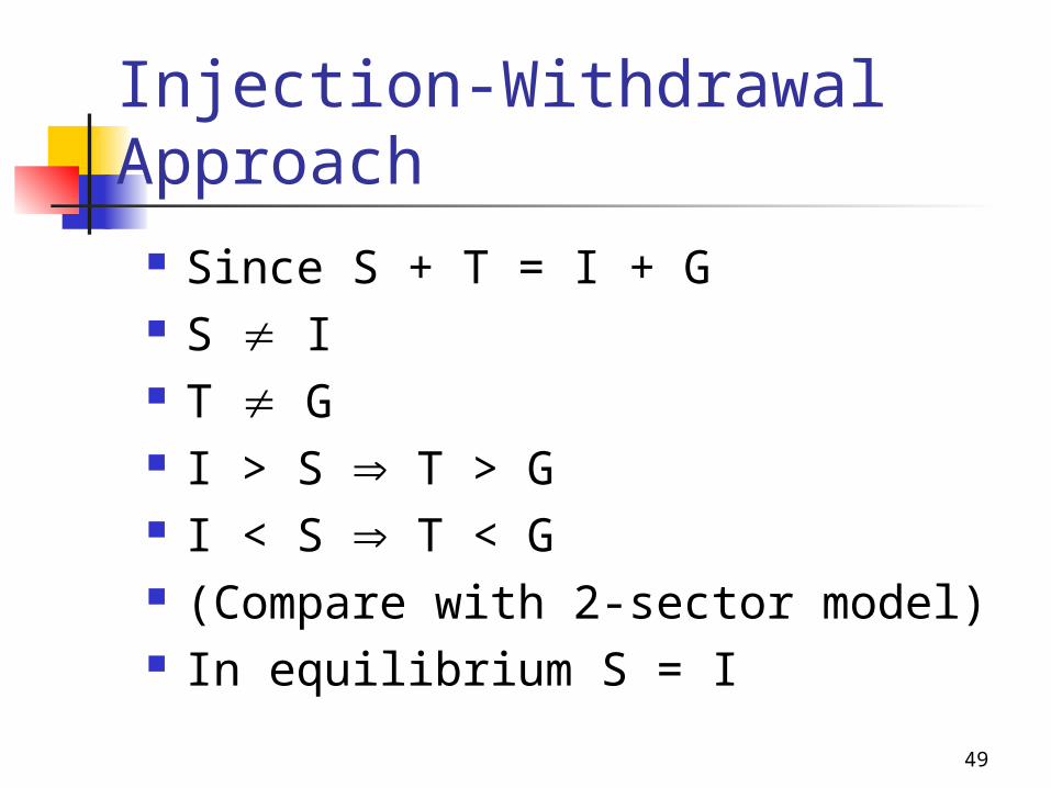
Injection-Withdrawal Approach
Since S + T = I + G S I T G I > S T > G I < S T < G (Compare with 2-sector model) In equilibrium S = I
50
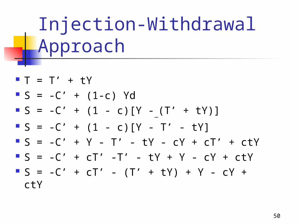
Injection-Withdrawal Approach
T = T’ + tY S = -C’ + (1-c) Yd S = -C’ + (1 - c)[Y -_(T’ + tY)] S = -C’ + (1 - c)[Y - T’ - tY] S = -C’ + Y - T’ - tY - cY + cT’ + ctY S = -C’ + cT’ -T’ - tY + Y - cY + ctY S = -C’ + cT’ - (T’ + tY) + Y - cY + ctY
51
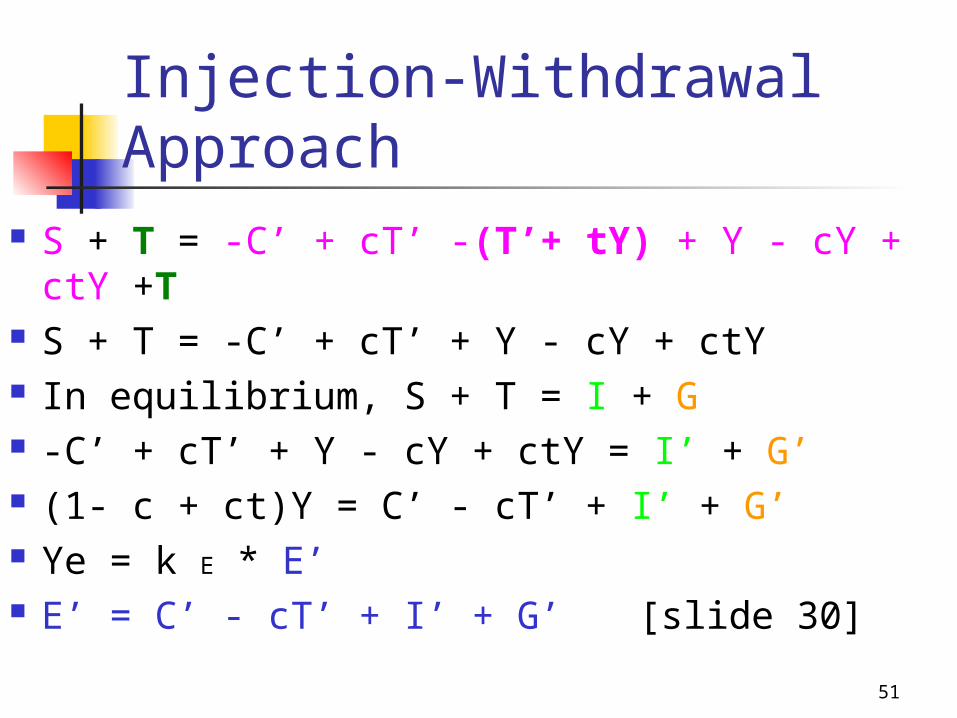
Injection-Withdrawal Approach
S + T = -C’ + cT’ -(T’+ tY) + Y - cY + ctY +T S + T = -C’ + cT’ + Y - cY + ctY In equilibrium, S + T = I + G -C’ + cT’ + Y - cY + ctY = I’ + G’ (1- c + ct)Y = C’ - cT’ + I’ + G’ Ye = k E * E’ E’ = C’ - cT’ + I’ + G’ [slide 30]
52
Use the Injection-Withdrawal Approach to solve for Ye if T=T’
53
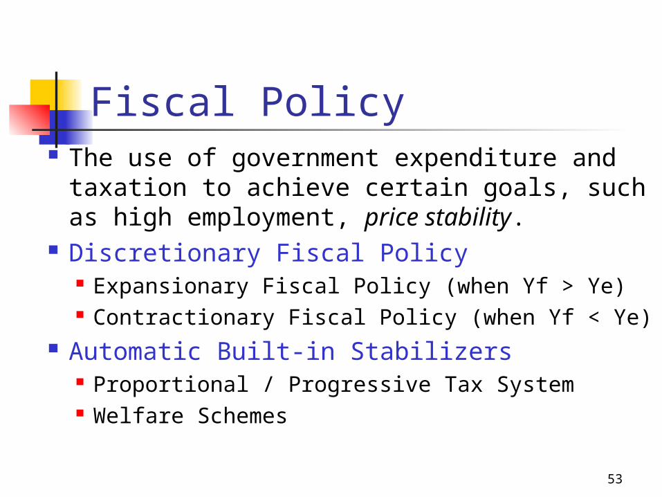
Fiscal Policy The use of government expenditure and
taxation to achieve certain goals, such as high employment, price stability.
Discretionary Fiscal Policy Expansionary Fiscal Policy (when Yf > Ye) Contractionary Fiscal Policy (when Yf < Ye)
Automatic Built-in Stabilizers Proportional / Progressive Tax System Welfare Schemes

54
Expansionary Fiscal Policy Recessionary/Deflationary Gap Yf-Ye
Y-line
E = E’ + (c -ct) Y
Ye
E = E” + (c-ct) Y
G’
Yf
Y= k E * E’
Recessionary Gap
G’ E’ E Y
55
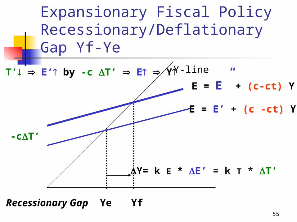
Expansionary Fiscal Policy Recessionary/Deflationary Gap Yf-Ye
Y-line
E = E’ + (c -ct) Y
Ye
E = E” + (c-ct) Y
-cT’
Yf
Y= k E * E’ = k T * T’
Recessionary Gap
T’ E’ by -c T’ E Y

56
Contractionary Fiscal PolicyInflationary Gap Ye - Yf
Y = E
E = E’ + (c-ct) Y
YeYf
E = E” + (c-ct) Y
Nominal Y>Yf Inflationary Gap
G’
G’ E’ E Y
Y= k E * E’
57
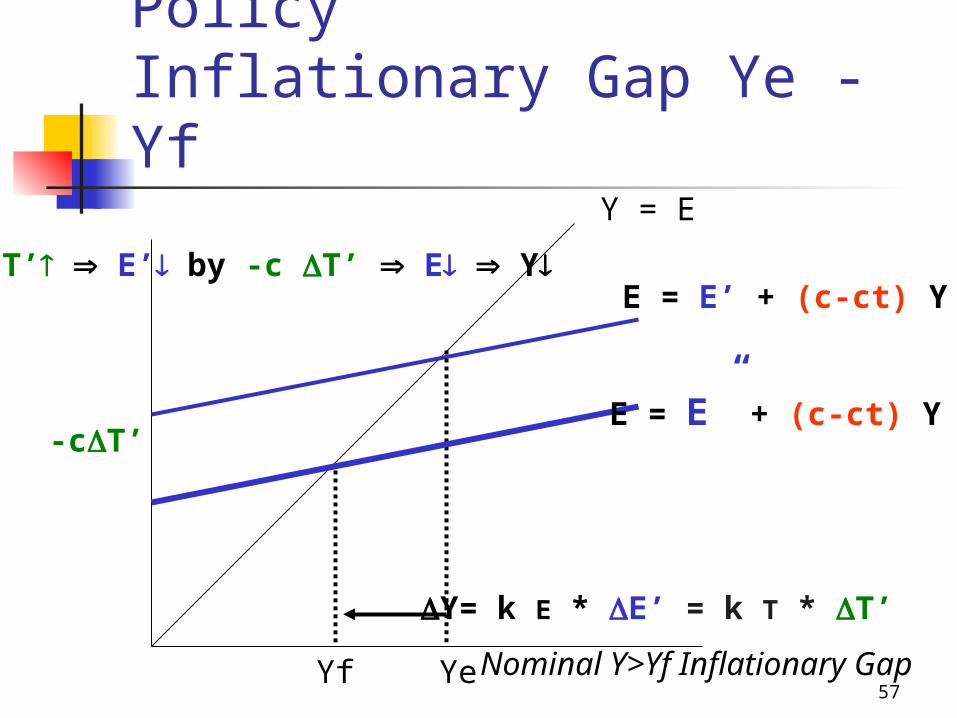
Contractionary Fiscal PolicyInflationary Gap Ye - Yf
Y = E
E = E’ + (c-ct) Y
YeYf
E = E” + (c-ct) Y
Nominal Y>Yf Inflationary Gap
-cT’
T’ E’ by -c T’ E Y
Y= k E * E’ = k T * T’
58
Automatic Built-in Stabilizers
Proportional /Progressive Tax System Recession: government’s tax revenue Boom: government’s tax revenue
The more progressive the tax system, the greater is its stabilizing effect. But there will be greater dis-incentives to earn income
With t, k E With proportional tax, the multiplying effect of a discretionary change in government expenditure G’ reduces

59
Automatic Built-in Stabilizers
Welfare Schemes Unemployment benefits, public
assistance allowances, agricultural support schemes Recession: government’s expenditure Boom: government’s expenditure
Again, if the welfare schemes are generous, the incentives to work will be weakened.
60
Discretionary Fiscal Policy v.s.Automatic Built-in Stabilizers
If the economy is close to Yf, built-in stabilizers are useful as they can stabilize the economy around Yf or potential income level.
However, if the economy is far below Yf, discretionary fiscal policy is still necessary (Simple Keynesian model).
Another drawback of the built-in stabilizers is they may reduce the speed of recovery as
k E Y = k E * E’
61
Discretionary Fiscal Policy Government expenditure G’? Tax T’? Location of effects If a recession is localized in a
particular industry G’ Tax cut will have its impact on the
entire economy
62
Discretionary Fiscal Policy Government expenditure G’? Tax T’? Duration of the time lag
Decision lag : time involved to assess a situation & decide what corrective actions should be taken
Executive lag : time involved to initiate corrective policies & for their full impact to be felt
tax cut has a much shorter executive lag
63
Discretionary Fiscal Policy Government expenditure G’? Tax T’? Reversibility of the fiscal policy
Government expenditure can easily be increased but are not so easy to cut as the civil servants who have vested interests in the present allocation of government expenditure will resist
Tax is easier to be changed as the civil servants who administer income tax is independent of the rate being levied. Of course, voter resistance should also be considered.
64
Discretionary Fiscal Policy Government expenditure G’? Tax T’? Public reaction to short-term changes A temporary tax cut raises Yd.
Households, recognizing this situation, may not revise their current consumption. Instead, they save a large part of the tax cut.
65
Financing the Government BudgetIncreasing Taxes
By increasing taxes, the government transfers purchasing power from current taxpayers to itself
Current taxpayers bear the cost If the revenue is spent on some investment
project, (current / future) taxpayers may benefit when the project is completed.
How about the revenue is spent on transfer payment?

66
Financing the Government BudgetPrinting more Money
This will create inflationary pressure. Households and firms will be able to
buy less with each unit of money. Fewer resources are available for private consumption and investment.
Those whose incomes respond slowly to changes in price levels will bear most of the cost of the government activity

67
Financing the Government BudgetInternal Debt
The government can transfer purchasing power from any willing lenders to itself in return for the promise to repay equivalent purchasing power plus interest in future.
Since, repayment of the debt are made from tax revenue, future taxpayers will suffer.
However, if the debt raised today is spent on creating capital assets, the burden on future generation will be lighter.
68
Financing the Government BudgetExternal Debt
Borrowing from abroad transfers purchasing power from foreigners to the government.
The burden on future generations will once again depend on how the debt raised is used (investment project / transfer payment)
69
The Problems of the Simple Keynesian Multiplier k E
Y = k E * G’ There are several problems with this
method of analysis, i.e., Y may be less Sources of financing G’ Effects on private investment I’ Productivity of government projects
70
The Problems of the Simple Keynesian Multiplier k E
Sources of financing G’ Increasing Tax
will exert a contractionary effect on the economy Increasing Money Supply
will generate an inflationary pressure Increasing Debt
will increase the demand for loanable fund as well as interest rate affect private investment
71
The Problems of the Simple Keynesian Multiplier k E
Effects on Private Investment I’ Private investment may be crowded out
when government increases its expenditure It is questionable that the government can
really produce something which is desired by the consumers
Besides, government investment projects are usually less productive than private investment projects
72
The Problems of the Simple Keynesian Multiplier k E Productivity of Government
Projects Government projects may not yield
a rate of return (MEC / MEI) exceeding the market interest rate.


![New Keynesian Model[1]](https://img.pdfslide.us/doc/110x75/577cd6701a28ab9e789c6177/new-keynesian-model1.jpg)