1

Noise Facilitation in Associative Memories ofExponential Capacity

Amin Karbasi, Amir Hesam Salavati, Amin Shokrollahi, and Lav R. Varshney

Abstract

Recent advances in associative memory design through structured pattern sets and graph-based inference al-gorithms have allowed reliable learning and recall of an exponential number of patterns. Although these designscorrect external errors in recall, they assume neurons that compute noiselessly, in contrast to the highly variableneurons in brain regions thought to operate associatively such as hippocampus and olfactory cortex.

Here we consider associative memories with noisy internal computations and analytically characterize perfor-mance. As long as the internal noise level is below a specified threshold, the error probability in the recall phasecan be made exceedingly small. More surprisingly, we show that internal noise actually improves the performanceof the recall phase while the pattern retrieval capacity remains intact, i.e., the number of stored patterns does notreduce with noise (up to a threshold). Computational experiments lend additional support to our theoretical analysis.This work suggests a functional benefit to noisy neurons in biological neuronal networks.

I. INTRODUCTION

BRAIN regions such as hippocampus and olfactory cortex are thought to operate as associative memories [2]–[4],having the ability to learn patterns from presented inputs, store a large number of patterns, and retrieve them

reliably in the face of noisy queries [5]–[7]. Mathematical models of associative memory are therefore designed tomemorize a set of given patterns so that corrupted versions of the memorized patterns may later be presented andthe correct memorized pattern retrieved.

Although such information storage and recall seemingly falls naturally into the information-theoretic framework[8], where an exponential number of messages can be communicated reliably using a linear number of symbols [9],classical associative memory models can only store a linear number of patterns with a linear number of symbols[6]. A primary shortcoming of such classical models has been their requirement to memorize a randomly chosenset of patterns. By enforcing structure and redundancy in the possible set of memorizable patterns—much likenatural stimuli [10], internal representations in neural systems [11], and codewords in error-control codes [12]—new advances in associative memory design allow storage of an exponential number of patterns with a linear numberof symbols [13], [14], just like in communication systems.1

Information-theoretic and associative memory models of storage have been used to predict experimentallymeasurable properties of synapses in the mammalian brain [16], [17]. But contrary to the fact that noise is presentin computational operations of the brain [18]–[22], associative memory models with exponential capacity haveassumed no internal noise in the computational nodes [14]; likewise with many classical models [5]. The purposeof the present paper is to model internal noise in associative memories with exponential pattern retrieval capacityand study whether they are still able to operate reliably. Surprisingly, we find internal noise actually enhances recallperformance without loss in capacity, thereby suggesting a functional role for variability in the brain.

In particular we consider a convolutional, graph code-based, associative memory model [14] and find that evenif all components are noisy, the final error probability in recall can be made exceedingly small. We characterizea threshold phenomenon and show how to optimize algorithm parameters when knowing statistical properties of

This work is based in part on a paper presented at the 2013 Neural Information Processing Systems Conference, Lake Tahoe, December2013 [1].

A. Karbasi is with Eidgenossische Technische Hochschule Zurich, Switzerland (e-mail: amin.karbasi@inf.ethz.ch).A. H. Salavati and A. Shokrollahi are with Ecole Polytechnique Federale de Lausanne, Switzerland (e-mail: {hesam.salavati,

amin.shokrollahi}@epfl.ch).L. R. Varshney was with the IBM Thomas J. Watson Research Center, NY. He is now with the University of Illinois at Urbana-Champaign

(e-mail: varshney@illinois.edu).1The idea of restricted pattern sets leading to associative memories with increased storage capacity was first suggested in an unpublished

doctoral dissertation [15].

arX

iv:1

403.

3305

v1 [

cs.N

E]

13

Mar

201

4

2

internal noise. Rather counterintuitively the performance of the memory model improves in the presence of internalneural noise, as has been observed previously as stochastic resonance in the literature [21], [23]. Deeper analysisshows mathematical connections to perturbed simplex algorithms for linear programing [24], where some internalnoise helps the algorithm get out of local minima.

A. Related Work

Designing neural networks to learn a set of patterns and recall them later in the presence of noise has beenan active topic of research for the past three decades. Inspired by Hebbian learning [25], Hopfield introduced anauto-associative neural mechanism of size n with binary state neurons in which patterns are assumed to be binaryvectors of length n [5]. The capacity of a Hopfield network under vanishing block error probability was latershown to be O(n/ log(n)) [6]. With the hope of increasing the capacity of the Hopfield network, extensions tonon-binary states were explored [7]. In particular, Jankowski et al. investigated a multi-state complex-valued neuralassociative memory with estimated capacity less than 0.15n [26]; Muezzinoglu et al. showed the capacity with aprohibitively complicated learning rule to increase to n [27]. Lee proposed the Modified Gradient Descent learningRule (MGDR) to overcome this drawback [28].

To further increase capacity and robustness, a recent line of work considers exploiting structure in patterns. Thisis done either by making use of correlations among patterns or by only memorizing patterns with redundancy(rather than any possible set of patterns). By utilizing neural cliques, [29] demonstrated that increasing the patternretrieval capacity of Hopfield networks to O(n2) is possible. Modification of neural architecture to improve patternretrieval capacity has also been previously considered by Venkatesh and Biswas [15], [30], where the capacity isincreased to Θ

(bn/b

)for semi-random patterns, where b = ω(lnn) is the size of clusters. This significant boost

to capacity is achieved by dividing the neural network into smaller fully interconnected disjoint blocks or nestedblocks (cf. [31]). This huge improvement comes at the price of limited worst-case noise tolerance capabilities.Deploying higher order neural models beyond the pairwise correlation considered in Hopfield networks increasesthe storage capacity to O(np−2), where p is the degree of correlation [32]. In such models, neuronal state dependsnot only on the state of neighbors, but also on the correlations among them. A new model based on bipartite graphsthat captures higher-order correlations (when patterns belong to a subspace), but without prohibitive computationalcomplexity, improved capacity to O(an), for some a > 1, that is to say exponential in network size [13].

The basic memory architecture, learning rule, and recall algorithm used herein is from [14], which also achievesexponential capacity by capturing internal redundancy by dividing the patterns into smaller overlapping clusters,with each subpattern satisfying a set of linear constraints. The problem of learning linear constraints with neuralnetworks was considered in [33], but without sparsity requirements. This has connections to compressed sensing[34]; typical compressed sensing recall/decoding algorithms are too complicated to be implemented by neuralnetworks, but some have suggested the biological plausibility of message-passing algorithms [35].

Building on the idea of structured pattern sets [29], the basic associative memory model used herein [14] relieson the fact all patterns to be learned lie in a low-dimensional subspace. Learning features of a low-dimensionalspace is very similar to autoencoders [36]. The model also has similarities to Deep Belief Networks (DBNs)and in particular Convolutional Neural Networks [37], albeit with different objectives. DBNs are made of severalconsecutive stages, similar to overlapping clusters in our model, where each stage extracts some features and feedsthem to the following stage. The output of the last stage is then used for pattern classification. In contrast to DBNs,our associative memory model is not classifying patterns but rather recalling patterns from noisy versions. Also,overlapping clusters can operate in parallel to save time in information diffusion over a staged architecture.

In most deep or convolutional models, one not only has to find the proper dictionary for classification, but alsocalculate the features for each input pattern. This increases the complexity of the whole system when the objectiveis simply recall. Here the dictionary corresponds to the dual vectors from previously memorized patterns.

In this work, we reconsider the neural network model of [14], but introduce internal computation noise consistentwith biology. Note that the sparsity of the model architecture is also consistent with biology [38]. We find thatthere is actually a functional benefit to internal noise.

The benefit of internal noise has been noted previously in associative memory models with stochastic updaterules, cf. [39], by analyzing attractor dynamics. In particular, it has been shown that noise may reduce recalltime in associative memory tasks by pushing the system from one attractor state to another [40]. However, our

3

framework differs from previous approaches in three key aspects. First, our memory model is different, whichmakes extension of previous analysis nontrivial. Second, and perhaps most importantly, pattern retrieval capacityin previous approaches decreases with internal noise, cf. [39, Figure 6.1], in that increasing internal noise helpscorrect more external errors, but also reduces the number of memorizable patterns. In our framework, internal noisedoes not affect pattern retrieval capacity (up to a threshold) but improves recall performance. Finally, our noisemodel has bounded rather than Gaussian noise, and so a suitable network may achieve perfect recall despite internalnoise.

Reliably storing information in memory systems constructed completely from unreliable components is a classicalproblem in fault-tolerant computing [41]–[43], where typical models have used random access architectures withsequential correcting networks. Although direct comparison is difficult since notions of circuit complexity areslightly different, our work also demonstrates that associative memory architectures can store information reliablydespite being constructed from unreliable components.

II. ASSOCIATIVE MEMORY MODEL

In this section, we introduce our main notation, the model of associative memories and noise. We also explainthe recall algorithms.

A. Notation and basic structure

In our model, a neuron can assume an integer-valued state from the set Q = {0, . . . , Q− 1}, interpreted as theshort term firing rate of neurons. A neuron updates its state based on the states of its neighbor {si}ni=1 as follows.It first computes a weighted sum h =

∑ni=1wisi + ζ, where wi is the weight of the link from si and ζ is the

internal noise, and then applies nonlinear function f : R→ Q to h.An associative memory is represented by a weighted bipartite graph, G, with pattern neurons and constraint

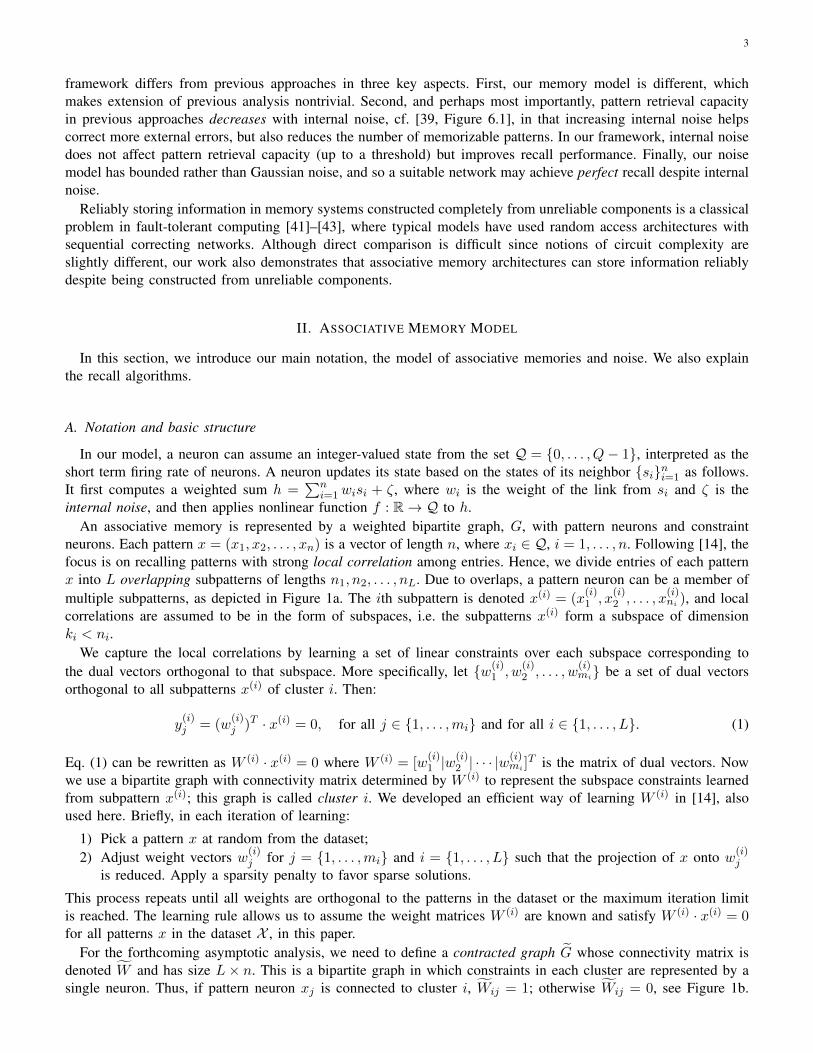
neurons. Each pattern x = (x1, x2, . . . , xn) is a vector of length n, where xi ∈ Q, i = 1, . . . , n. Following [14], thefocus is on recalling patterns with strong local correlation among entries. Hence, we divide entries of each patternx into L overlapping subpatterns of lengths n1, n2, . . . , nL. Due to overlaps, a pattern neuron can be a member ofmultiple subpatterns, as depicted in Figure 1a. The ith subpattern is denoted x(i) = (x

(i)1 , x

(i)2 , . . . , x

(i)ni ), and local

correlations are assumed to be in the form of subspaces, i.e. the subpatterns x(i) form a subspace of dimensionki < ni.

We capture the local correlations by learning a set of linear constraints over each subspace corresponding tothe dual vectors orthogonal to that subspace. More specifically, let {w(i)

1 , w(i)2 , . . . , w

(i)mi} be a set of dual vectors

orthogonal to all subpatterns x(i) of cluster i. Then:

y(i)j = (w

(i)j )T · x(i) = 0, for all j ∈ {1, . . . ,mi} and for all i ∈ {1, . . . , L}. (1)

Eq. (1) can be rewritten as W (i) · x(i) = 0 where W (i) = [w(i)1 |w

(i)2 | · · · |w

(i)mi ]

T is the matrix of dual vectors. Nowwe use a bipartite graph with connectivity matrix determined by W (i) to represent the subspace constraints learnedfrom subpattern x(i); this graph is called cluster i. We developed an efficient way of learning W (i) in [14], alsoused here. Briefly, in each iteration of learning:

1) Pick a pattern x at random from the dataset;2) Adjust weight vectors w(i)

j for j = {1, . . . ,mi} and i = {1, . . . , L} such that the projection of x onto w(i)j

is reduced. Apply a sparsity penalty to favor sparse solutions.

This process repeats until all weights are orthogonal to the patterns in the dataset or the maximum iteration limitis reached. The learning rule allows us to assume the weight matrices W (i) are known and satisfy W (i) · x(i) = 0for all patterns x in the dataset X , in this paper.

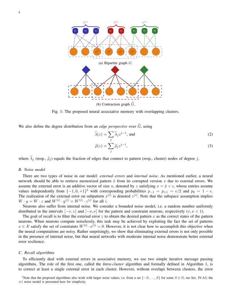
For the forthcoming asymptotic analysis, we need to define a contracted graph G whose connectivity matrix isdenoted W and has size L× n. This is a bipartite graph in which constraints in each cluster are represented by asingle neuron. Thus, if pattern neuron xj is connected to cluster i, Wij = 1; otherwise Wij = 0, see Figure 1b.

4

y1 y2 y3

x(2)1

G(1)

y4 y5

x(2)2 x

(2)3

G(2)

y6 y7 y8

x(2)4

G(3)

(a) Bipartite graph G.

(b) Contraction graph G.

Fig. 1: The proposed neural associative memory with overlapping clusters.

We also define the degree distribution from an edge perspective over G, using

λ(z) =∑j

λjzj−1, and (2)

ρ(z) =∑j

ρjzj−1, (3)

where λj (resp., ρj) equals the fraction of edges that connect to pattern (resp., cluster) nodes of degree j.

B. Noise model

There are two types of noise in our model: external errors and internal noise. As mentioned earlier, a neuralnetwork should be able to retrieve memorized pattern x from its corrupted version x due to external errors. Weassume the external error is an additive vector of size n, denoted by z satisfying x = x+ z, whose entries assumevalues independently from {−1, 0,+1}2 with corresponding probabilities p−1 = p+1 = ε/2 and p0 = 1 − ε.The realization of the external error on subpattern x(i) is denoted z(i). Note that the subspace assumption impliesW · y = W · z and W (i) · y(i) = W (i) · z(i) for all i.

Neurons also suffer from internal noise. We consider a bounded noise model, i.e. a random number uniformlydistributed in the intervals [−υ, υ] and [−ν, ν] for the pattern and constraint neurons, respectively (υ, ν < 1).

The goal of recall is to filter the external error z to obtain the desired pattern x as the correct states of the patternneurons. When neurons compute noiselessly, this task may be achieved by exploiting the fact the set of patternsx ∈ X satisfy the set of constraints W (i) ·x(i) = 0. However, it is not clear how to accomplish this objective whenthe neural computations are noisy. Rather surprisingly, we show that eliminating external errors is not only possiblein the presence of internal noise, but that neural networks with moderate internal noise demonstrate better externalerror resilience.

C. Recall algorithms

To efficiently deal with external errors in associative memory, we use two simple iterative message passingalgorithms. The role of the first one, called the Intra-cluster algorithm and formally defined in Algorithm 1, isto correct at least a single external error in each cluster. However, without overlaps between clusters, the error

2Note that the proposed algorithms also work with larger noise values, i.e. from a set {−S, . . . , S} for some S ∈ N, see Sec. IV-A2; the±1 noise model is presented here for simplicity.

5

resilience of this approach and the network in general is limited. The second algorithm, the Inter-cluster recallalgorithm, exploits the overlaps: it helps clusters with external errors recover their correct states by using thereliable information from clusters that do not have external errors. The error resilience of the resulting combinationthereby drastically improves.

To go further into details, and with abuse of notations, let xi(t) and yj(t) denote the message transmitted atiteration t by pattern and constraint neurons, respectively. In the first iteration, we initialize the pattern neuronswith a pattern randomly drawn from the dataset, x, corrupted with some external noise, z. Thus, x(0) = x+ z. Asa result, for cluster ` we have x(`)(0) = x(`) + z(`), where z(`) is the realization of the external error on cluster `.

With these notations in mind, Algorithm 1 iteratively performs a series of forward and backward steps in orderto remove (at least) one external error from its input domain. Assuming that the algorithm is applied to cluster `,in the forward step of iteration t the pattern neurons in cluster ` transmit their current states to their neighboringconstraint neurons. Each constraint neuron j then calculates the weighted sum of the messages it received over itsinput links. Nevertheless, since neurons suffer from internal noise, additional noise terms appear in the weightedsum, i.e., h(`)j =

∑n`

i=1W(`)ij x

(`)i +vi, where vi is the random internal noise affecting node i. As before, we consider

a bounded noise model for vi, i.e., it is uniformly distributed in the interval [−ν, ν] for some ν < 1.A non-zero input sum, excluding the effect of vi, is an indication of the presence of external errors among the

pattern neurons. Thus, constraint neurons set to their states to the sign of the received weighted sum if its magnitudeis larger than a fixed threshold, ψ. More specifically, constraint neuron j updates its state based on the receivedweighted sum according to the following rule

y(`)j (t) = f(h

(`)j (t), ψ) =

+1, if h(`)j (t) ≥ ψ0, if − ψ ≤ h(`)j (t) ≤ ψ−1, otherwise,

(4)

Here, x(`)(t) = [x(`)1 (t), . . . , x

(`)n` (t)] is the vector of messages transmitted by the pattern neurons and vi is the

random internal noise affecting node i.3

In the backward step, the constraint neurons communicate their states to their neighboring pattern neurons. Thepattern neurons then compute a normalized weighted sum on the messages they receive over their input link andupdate their current state if the amount of received (non-zero) feedback exceeds a threshold. Otherwise, they willretain their current state for the next round. More specifically, pattern node i in cluster ` updates its state in roundt according to the equation below

x(`)i (t+ 1) =

{x(`)i (t)− sign(g

(`)i (t)), if |g(`)i (t)| ≥ ϕ

x(`)i (t), otherwise,

(5)

where ϕ is the update threshold and

g(`)i (t) =

((sign(W (`))> · y(`)(t)

)i

d(`)i

+ ui.

Note that x(`)i (t+1) is further mapped to the interval [0, Q−1] by saturating the values below 0 and above Q−1 to0 and Q− 1 respectively; this saturation is not stated mathematically for brevity. Here, d(`)i is the degree of patternnode i in cluster `, y(`)(t) = [y

(`)1 (t), . . . , y

(`)m`(t)] is the vector of messages transmitted by the constraint neurons

in cluster `, and ui is the random internal noise affecting pattern node i. Basically, the term g(`)i (t) reflects the

(average) belief of constraint nodes connected to pattern neuron i about its correct value. If g(`)i (t) is larger thana specified threshold ϕ it means most of the connected constraints suggest the current state x(`)i (t) is not correct,hence, a change should be made. Note this average belief is diluted by the internal noise of neuron i. As mentionedearlier, ui is uniformly distributed in the interval [−υ, υ], for some υ < 1.

The error correction ability of Algorithm 1 is fairly limited, as determined analytically and through simulations inthe sequel. In essence, Algorithm 1 can correct one external error with high probability, but degrades terribly against

3Note that although the values of y(`)i (t) can be shifted to 0, 1, 2, instead of −1, 0, 1 to match our assumption that neural states arenon-negative, we leave them as such to simplify later analysis.

6

Algorithm 1 Intra-Module Error CorrectionInput: Training set X , thresholds ϕ,ψ, iteration tmax

Output: x(`)1 , x(`)2 , . . . , x

(`)n`

1: for t = 1→ tmax do2: Forward iteration: Calculate the input h(`)i =

∑n`

j=1W(`)ij x

(`)j + vi, for each neuron y

(`)i and set y(`)i =

f(h(`)i , ψ).

3: Backward iteration: Each neuron x(`)j computes

g(`)j =

∑m`i=1 sign(W (`)

ij )y(`)i∑m`

i=1 sign(|W (`)ij |)

+ ui.

4: Update the state of each pattern neuron j according to x(`)j = x(`)j − sign(g

(`)j ) only if |g(`)j | > ϕ.

5: end for

Algorithm 2 Sequential Peeling Algorithm

Input: G,G(1), G(2), . . . , G(L).Output: x1, x2, . . . , xn

1: while there is an unsatisfied v(`) do2: for ` = 1→ L do3: If v(`) is unsatisfied, apply Algorithm 1 to cluster G(l).4: If v(`) remained unsatisfied, revert the state of pattern neurons connected to v(`) to their initial state.

Otherwise, keep their current states.5: end for6: end while7: Declare x1, x2, . . . , xn if all v(`)’s are satisfied. Otherwise, declare failure.

two or more external errors. Working independently, clusters cannot correct more than a few external errors, buttheir combined performance is much better. As clusters overlap, they help each other in resolving external errors:a cluster whose pattern neurons are in their correct states can always provide truthful information to neighboringclusters. This property is exploited in Algorithm 2 by applying Algorithm 1 in a round-robin fashion to eachcluster. Clusters either eliminate their internal noise in which case they keep their new states and can now helpother clusters, or revert back to their original states. Note that by such a scheduling scheme, neurons can onlychange their states towards correct values. This scheduling technique is similar in spirit to the peeling algorithm[44].

III. PATTERN RETRIEVAL CAPACITY

Before proceeding to analyze recall performance, for completeness we review pattern retrieval capacity resultsfrom [14] to show that the proposed model is capable of memorizing an exponentially large number of patterns.First, note that since the patterns form a subspace, the number of patterns C does not have any effect on thelearning or recall algorithms (except for its obvious influence on the learning time). Thus, in order to show thatthe pattern retrieval capacity is exponential in n, all we need to demonstrate is that there exists a training set Xwith C patterns of length n for which C ∝ arn, for some a > 1 and 0 < r.

Theorem 1 ( [14]). Let X be a C × n matrix, formed by C vectors of length n with entries from the set Q.Furthermore, let k = rn for some 0 < r < 1. Then, there exists a set of vectors for which C = arn, with a > 1,and rank(X ) = k < n.

The proof is constructive: we create a dataset X such that it can be memorized by the proposed neural network

7

and satisfies the required properties, i.e. the subpatterns form a subspace and pattern entries are integer values fromthe set Q = {0, . . . , Q− 1}. The complete proof can be found in [14].

IV. RECALL PERFORMANCE ANALYSIS

Now let us analyze recall error performance. The following lemma shows that if ϕ and ψ are chosen properly,then in the absence of external errors the constraints remain satisfied and internal noise cannot result in violations.This is a crucial property for Algorithm 2, as it allows one to determine whether a cluster has successfully eliminatedexternal errors (Step 4 of algorithm) by merely checking the satisfaction of all constraint nodes.

Lemma 1. In the absence of external errors, the probability that a constraint neuron (resp. pattern neuron) in cluster` makes a wrong decision due to its internal noise is given by π(`)0 = max

(0, ν−ψν

)(resp. P (`)

0 = max(0, υ−ϕυ

)).

Proof: To calculate the probability that a constraint node makes a mistake when there are no external errors,consider constraint node i whose decision parameter will be

h(`)i =

(W (`) · x(`)

)i+ vi = vi.

Therefore, the probability of making a mistake will be

π(`)0 = Pr{|vi| > ψ} = max

(0,ν − ψν

). (6)

Thus, to make π(`)0 = 0 we will select ψ > ν. Note that this might not be possible in all cases since, as we willsee, the minimum absolute value of network weights should be at least ψ; if ψ is too large we might not be ableto find a proper set of weights. Nevertheless, and assuming that it is possible to choose a proper ψ, we will have

π(0) = 0. (7)

Now knowing that the constraint will not send any non-zero messages in the absence of external noise, wefocus on the pattern neurons in the same circumstance. A given pattern node x(`)j will receive a zero from all its

neighbors among the constraint nodes. Therefore, its decision parameter will be g(`)j = uj . As a result, a mistakecould happen if |uj | ≥ ϕ. The probability of this event is given by

P(`)0 = Pr{|ui| > ϕ} = max

(0,υ − ϕϕ

). (8)

Therefore, to make P (`)0 go to zero, we must select ϕ ≥ υ.

In the sequel, we assume ϕ > υ and ψ > ν so that π(`)0 = 0 and P (`)0 = 0. However, an external error combined

with internal noise may still push neurons to an incorrect state.Given the above lemma and our neural architecture, we can prove the following surprising result: in the asymptotic

regime of increasing number of iterations of Algorithm 2, a neural network with internal noise outperforms onewithout, with the pattern retrieval capacity remaining intact. Let us define the fraction of errors corrected by thenoiseless and noisy neural network (parametrized by υ and ν) after T iterations of Algorithm 2 by Λ(T ) andΛυ,ν(T ), respectively. Note that both Λ(T ) ≤ 1 and Λυ,ν(T ) ≤ 1 are non-decreasing sequences of T . Hence, theirlimiting values are well defined: limT→∞ Λ(T ) = Λ∗ and limT→∞ Λυ,ν(T ) = Λ∗υ,ν .

Theorem 2. Let us choose ϕ and ψ so that π(`)0 = 0 and P (`)0 = 0 for all ` ∈ {1, . . . , L}. For the same realization

of external errors, we have Λ∗υ,ν ≥ Λ∗.

Proof: We first show that the noisy network can correct any external error pattern that the noiseless counterpartcan correct in the T →∞ limit. If the noiseless decoder succeeds, then there is a non-zero probability P that thenoisy decoder succeeds in a given round as well (corresponding to the case that noise values are rather small).Since we do not introduce new errors during the application of Algorithm 2, the number of errors in the newrounds are smaller than or equal to the previous round, hence the probability of success is lower bounded by P .If Algorithm 2 is applied T times, then the probability of correcting the external errors at the end of round T isP + P (1− P ) + · · ·+ P (1− P )T−1 = 1− (1− P )T . Since P > 0, for T →∞ this probability tends to 1.

8

Now, we turn attention to cases where the noiseless network fails in eliminating external errors and show thatthere exist external error patterns, called stopping sets, for which the noisy network is capable of eliminating themwhile the noiseless network has failed; see Appendix A for further explication. Assuming that each cluster caneliminate i external errors in their domain and in the absence of internal noise,4 stopping sets correspond to noisepatterns in which each cluster has more than i errors. Then Algorithm 2 cannot proceed any further. However, inthe noisy network, there is a chance that in one of the rounds, the noise acts in favorably and the cluster couldcorrect more than i errors.5 In this case, if the probability of getting out of the stopping set is P in each round,for some P > 0, then a similar argument to the previous case shows that P → 1 when T →∞.

It should be noted that if the amount of internal noise or external errors is too high, the noisy architecture willeventually get stuck just like the noiseless network. The high level idea why a noisy network outperforms a noiselessone comes from understanding stopping sets, realizations of external errors where the iterative Algorithm 2 cannotcorrect them all. We showed that the stopping set shrinks as we add internal noise and so the supposedly harmfulinternal noise helps Algorithm 2 to avoid stopping sets. Appendix A illustrates this notion further.

Theorem 2 suggests the only possible downside to using a noisy network is its possible running time in eliminatingexternal errors: the noisy neural network may need more iterations to achieve the same error correction performance.Interestingly, our empirical experiments show that in certain scenarios, even the running time improves when usinga noisy network.

Theorem 2 indicates that noisy neural networks (under our model) outperform noiseless ones, but does not specifythe level of errors that such networks can correct. Now we derive a theoretical upper bound on error correctionperformance. To this end, let Pci be the average probability that a cluster can correct i external errors in its domain.The following theorem gives a simple condition under which Algorithm 2 can correct a linear fraction of externalerrors (in terms of n) with high probability. The condition involves λ and ρ, the degree distributions of the contractedgraph G.

Theorem 3. Under the assumptions that graph G grows large and it is chosen randomly with degree distributionsgiven by λ and ρ, Algorithm 2 is successful if

ελ

1−∑i≥1

Pcizi−1

i!· d

i−1ρ(1− z)dzi−1

< z, for z ∈ [0, ε]. (9)

Proof: The proof is based on the density evolution technique [12]. Without loss of generality, assume we havePc1 , Pc2 , and Pc3 (and Pci = 0 for i > 3.) but the proof can easily be extended if we have Pci for i > 3. Let Π(t)be the average probability that a super constraint node sends a failure message, i.e., that it can not correct externalerrors lying in its domain. Then, the probability that a noisy pattern neuron with degree di sends an erroneousmessage to a particular neighbor among super constraint node is equal to the probability that none of its otherneighboring super constraint nodes could have corrected its error, i.e.,

Pi(t) = pe(Π(t))di−1.

Averaging over di we find the average probability of error in iteration t:

z(t+ 1) = peλ(Π(t)). (10)

Now consider a cluster ` that contains d` pattern neurons. This cluster will not send a failure message over itsedge to a noisy pattern neuron in its domain with probability:

1) Pc1 , if it is not connected to any other noisy neuron;2) Pc2 , if it is connected to exactly one other constraint neuron;3) Pc3 , if it is connected to exactly two other constraint neurons; and4) 0, if it is connected to more than two other constraint neuron.

Thus,

Π(`)(t) = 1− Pc1 (1− z(t))d`−1 − Pc2(d` − 1

1

)z(t) (1− z(t))d`−2 − Pc3

(d` − 1

2

)z(t)2 (1− z(t))d`−3 .

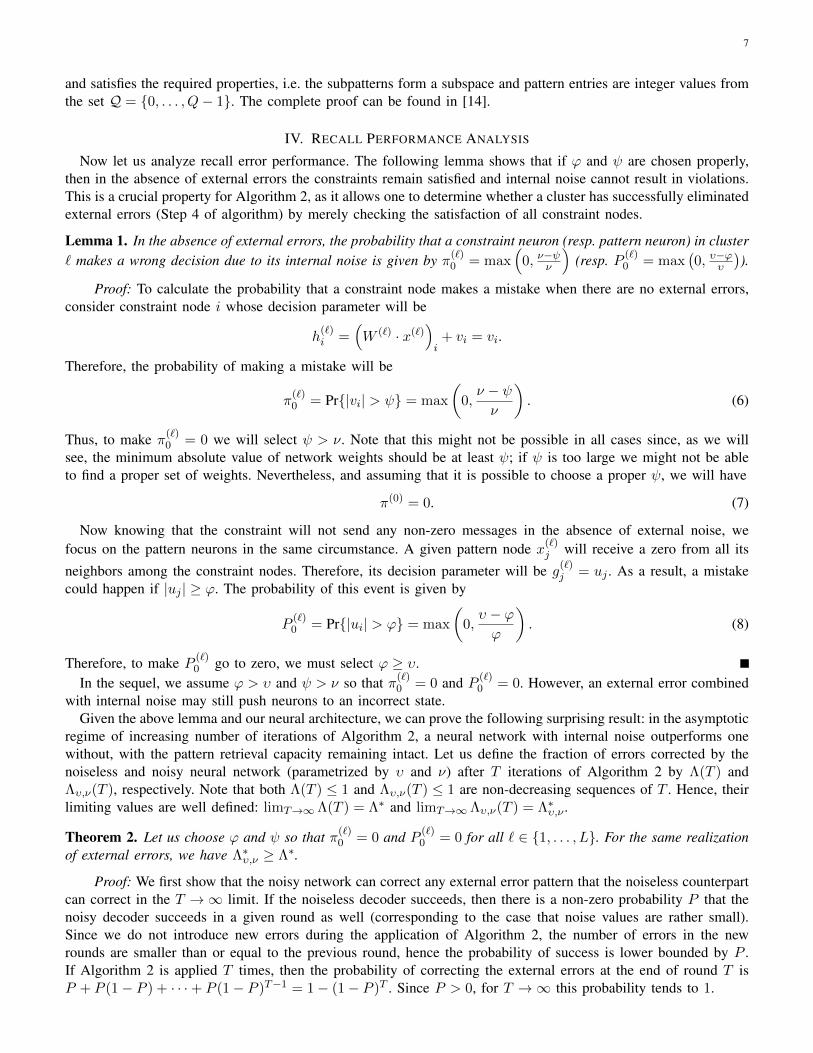
4From the forthcoming Figure 2, we will see that i = 2 in this case.5This is reflected in the forthcoming Figure 2, where the value of Pci is larger when the network is noisy.

9

0 0.1 0.2 0.3 0.4 0.5 0.6 0.70

0.2

0.4

0.6

0.8

1

υ

Prob

abili

tyof

corr

ectin

gex

tern

aler

rors Pc1

Pc2

Pc3

Pc4

Fig. 2: The value of Pci as a function of pattern neurons noise υ for i = 1, . . . , 4. The noise at constraint neuronsis assumed to be zero (ν = 0).

Averaging over d` yields:

Π(t) = Ed`(

Π(`)(t))

= 1− Pc1ρ(1− z(t))− Pc2zρ′(1− z(t))− 12Pc2z(t)

2ρ′′ (1− z(t)) , (11)

where ρ′(x) and ρ′′(x) are derivatives of the function ρ(x) with respect to x.Equations (10) and (11) yield the value of z(t+ 1) as a function of z(t). We calculate the final error probability

as limt→∞ z(t); for limt→∞ z(t)→ 0, it is sufficient to have z(t+ 1) < z(t), which proves the theorem.It must be mentioned that the above theorem holds when the decision subgraphs for the pattern neurons in graph

G are tree-like for a depth of τL, where τ is the total number of number of iterations performed by Algorithm 2[12].

Theorem 3 states that for any fraction of errors Λυ,ν ≤ Λ∗υ,ν that satisfies the above recursive formula, Algorithm 2will be successful with probability close to one. Note that the first fixed point of the above recursive equation dictatesthe maximum fraction of errors Λ∗υ,ν that our model can correct. For the special case of Pc1 = 1 and Pci = 0, forall i > 1, we obtain ελ (1− ρ(1− z)) < z, the same condition given in [14]. Theorem 3 takes into account thecontribution of all Pci terms and as we will see, their values change as we incorporate the effect of internal noise υand ν. Our results show that the maximum value of Pci does not occur when the internal noise is equal to zero, i.e.υ = ν = 0, but instead when the neurons are contaminated with internal noise! As an example, Figure 2 illustrateshow Pci behaves as a function of υ in the network considered (note that maximum values are not at υ = 0). Thisfinding suggests that even individual clusters are able to correct more errors in the presence of internal noise.

To estimate the Pci values, we use numerical approaches.6 Given a set of clusters W (1), . . . ,W (L), for eachcluster we randomly corrupt i pattern neurons with ±1 noise. Then, we apply Algorithm 1 over this cluster andcalculate the success rate once finished. We take the average of this rate over all clusters to end up with Pci . Theresults of this approach are shown in Figure 2, where the value of Pci is shown for i = 1, . . . , 4 and various noiseamounts at the pattern neurons (specified by parameter υ).

A. Simulations

Now we consider simulation results for a finite system. To learn the subspace constraints (1) for each cluster G(`)

we use the learning algorithm in [14]. Henceforth, we assume that the weight matrix W is known and given. In oursetup, we consider a network of size n = 400 with L = 50 clusters. We have 40 pattern nodes and 20 constraint

6Appendix B derives an analytical upper bound to estimate Pc1 but this requires approximations that are loose.

10

0.00 0.05 0.100.00

0.05

0.10

0.15

ǫ

Fina

lSE

R

υ = 0, ν = 0-Simυ = 0, ν = 0-Thrυ = 0.2, ν = 0-Simυ = 0.2, ν = 0-Thrυ = 0.4, ν = 0-Simυ = 0.4, ν = 0-Thrυ = 0.6, ν = 0-Simυ = 0.6, ν = 0-Thr

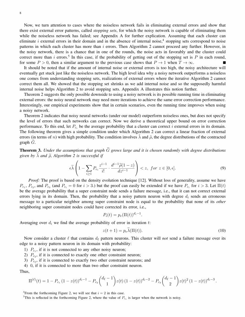
Fig. 3: The final SER for a network with n = 400, L = 50. The red curves correspond to the noiseless neuralnetwork.

nodes in each cluster, on average. External error is modeled by randomly generated vectors z with entries ±1 withprobability ε and 0 otherwise. Vector z is added to the correct patterns, which satisfy (1). For recall, Algorithm 2is used and results are reported in terms of Symbol Error Rate (SER) as the level of external error (ε) or internalnoise (υ, ν) is changed; this involves counting positions where the output of Algorithm 2 differs from the correctpattern.

1) Symbol Error Rate as a function of Internal Noise: Figure 3 illustrates the final SER of our algorithm fordifferent values of υ and ν. Remember that υ and ν quantify the level of noise in pattern and constraint neurons,respectively. Dashed lines in Figure 3 are simulation results whereas solid lines are theoretical upper boundsprovided in this paper. As evident, there is a threshold phenomenon such that SER is negligible for ε ≤ ε∗ andgrows beyond this threshold. As expected, simulation results are better than the theoretical bounds. In particular,the gap is relatively large as υ moves towards one.

A more interesting trend in Figure 3 is the fact that internal noise helps in achieving better performance, aspredicted by theoretical analysis (Theorem 2). Notice how ε∗ moves towards one as ν increases.

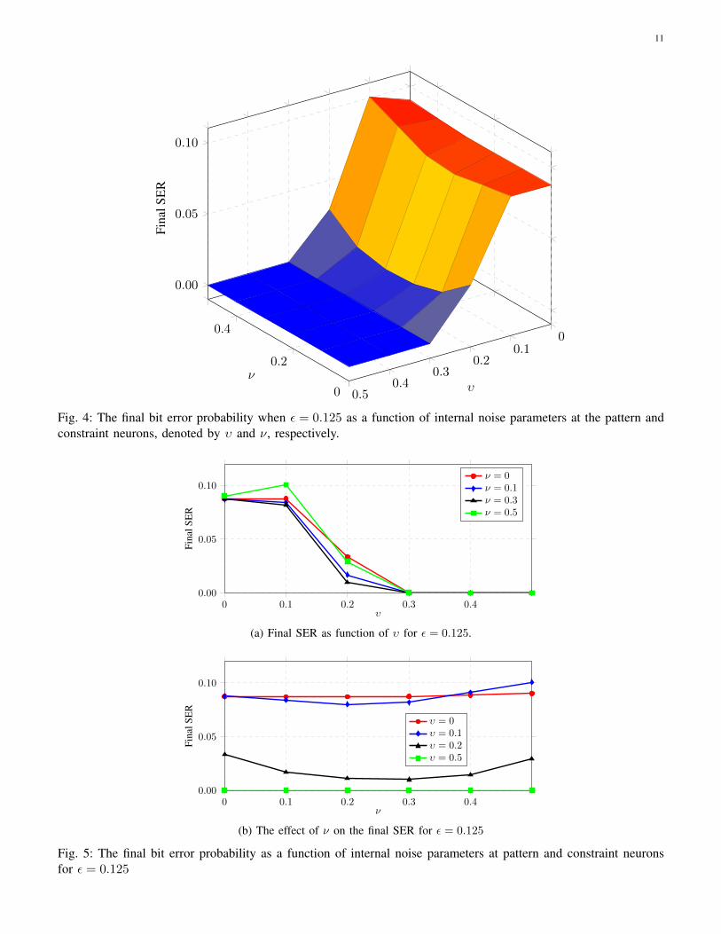
This phenomenon is inspected more closely in Figure 4 where ε is fixed to 0.125 while υ and ν vary. Figs. 5aand 5b display projected versions of the surface plot to investigate the effect of υ and ν separately. As we seeagain, a moderate amount of internal noise at both pattern and constraint neurons improves performance. There isan optimum point (υ∗, ν∗) for which the SER reaches its minimum. Figure 5b indicates for instance that ν∗ ≈ 0.25,beyond which SER deteriorates. There is greater sensitivity to noise υ in the pattern neurons, reminiscent of resultsfor decoding circuits with internal noise [45].

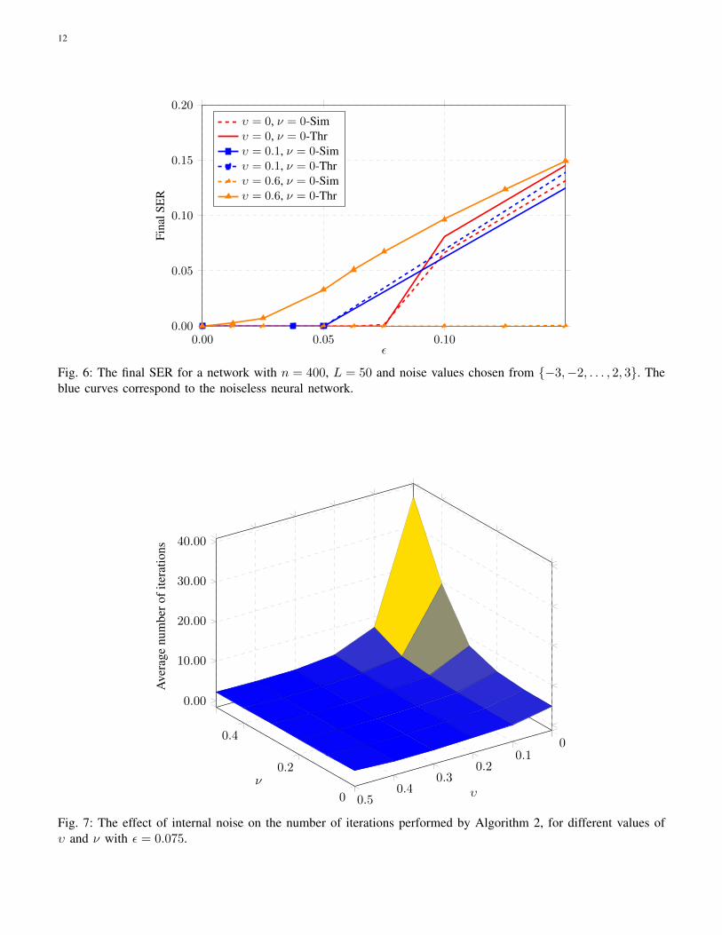
2) Larger noise values: So far, we have investigated the performance of the recall algorithm when noise valuesare limited to ±1. Although this choice facilitates the analysis of the algorithm and increases error correction speed,our analysis is valid for larger noise values. Figure 6 illustrates the SER for the same scenario as before but withnoise values chosen from {−3,−2, . . . , 2, 3}. We see exactly the same behavior as we witnessed for ±1 noisevalues.

B. Recall Time as a function of Internal Noise

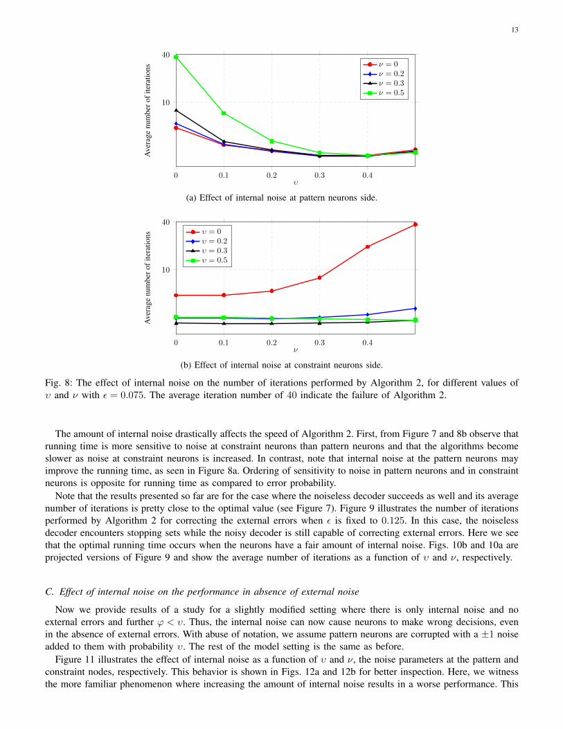
Figure 7 illustrates the number of iterations performed by Algorithm 2 for correcting the external errors when εis fixed to 0.075. We stop whenever the algorithm corrects all external errors or declare a recall error if all errorswere not corrected in 40 iterations. Thus, the corresponding areas in the figure where the number of iterationsreaches 40 indicates decoding failure. Figs. 8a and 8b are projected versions of Figure 7 and show the averagenumber of iterations as a function of υ and ν, respectively.

11

0

0.2

0.40

0.10.2

0.30.4

0.5

0.00

0.05

0.10

νυ

Fina

lSE

R

Fig. 4: The final bit error probability when ε = 0.125 as a function of internal noise parameters at the pattern andconstraint neurons, denoted by υ and ν, respectively.

0 0.1 0.2 0.3 0.40.00

0.05

0.10

υ

Fina

lSE

R

ν = 0ν = 0.1ν = 0.3ν = 0.5

(a) Final SER as function of υ for ε = 0.125.

0 0.1 0.2 0.3 0.40.00

0.05

0.10

ν

Fina

lSE

R

υ = 0υ = 0.1υ = 0.2υ = 0.5

(b) The effect of ν on the final SER for ε = 0.125

Fig. 5: The final bit error probability as a function of internal noise parameters at pattern and constraint neuronsfor ε = 0.125

12

0.00 0.05 0.100.00

0.05

0.10

0.15

0.20

ǫ

Fina

lSE

R

υ = 0, ν = 0-Simυ = 0, ν = 0-Thrυ = 0.1, ν = 0-Simυ = 0.1, ν = 0-Thrυ = 0.6, ν = 0-Simυ = 0.6, ν = 0-Thr

Fig. 6: The final SER for a network with n = 400, L = 50 and noise values chosen from {−3,−2, . . . , 2, 3}. Theblue curves correspond to the noiseless neural network.

0

0.2

0.40

0.10.2

0.30.4

0.5

0.00

10.00

20.00

30.00

40.00

νυ

Ave

rage

num

bero

fite

ratio

ns

Fig. 7: The effect of internal noise on the number of iterations performed by Algorithm 2, for different values ofυ and ν with ε = 0.075.

13

0 0.1 0.2 0.3 0.4

10

40

υ

Ave

rage

num

bero

fite

ratio

ns ν = 0ν = 0.2ν = 0.3ν = 0.5

(a) Effect of internal noise at pattern neurons side.

0 0.1 0.2 0.3 0.4

10

40

ν

Ave

rage

num

bero

fite

ratio

ns υ = 0υ = 0.2υ = 0.3υ = 0.5

(b) Effect of internal noise at constraint neurons side.

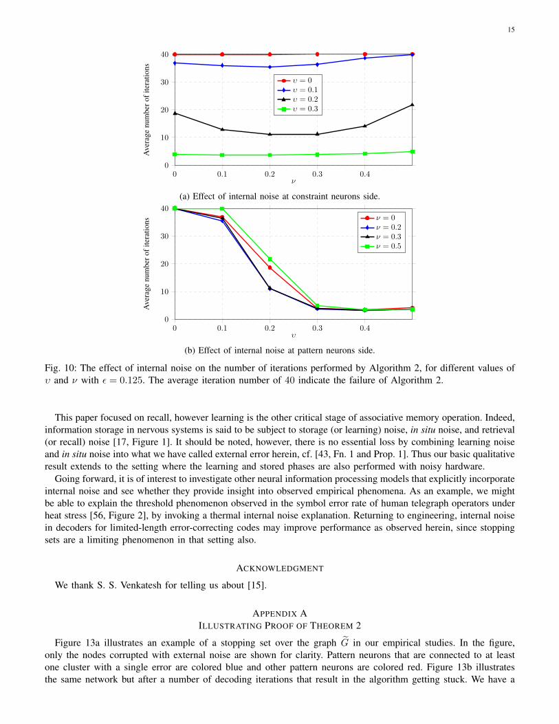
Fig. 8: The effect of internal noise on the number of iterations performed by Algorithm 2, for different values ofυ and ν with ε = 0.075. The average iteration number of 40 indicate the failure of Algorithm 2.

The amount of internal noise drastically affects the speed of Algorithm 2. First, from Figure 7 and 8b observe thatrunning time is more sensitive to noise at constraint neurons than pattern neurons and that the algorithms becomeslower as noise at constraint neurons is increased. In contrast, note that internal noise at the pattern neurons mayimprove the running time, as seen in Figure 8a. Ordering of sensitivity to noise in pattern neurons and in constraintneurons is opposite for running time as compared to error probability.

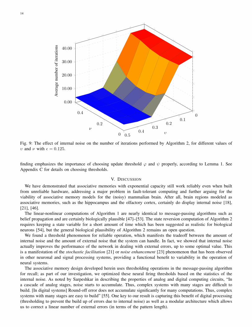
Note that the results presented so far are for the case where the noiseless decoder succeeds as well and its averagenumber of iterations is pretty close to the optimal value (see Figure 7). Figure 9 illustrates the number of iterationsperformed by Algorithm 2 for correcting the external errors when ε is fixed to 0.125. In this case, the noiselessdecoder encounters stopping sets while the noisy decoder is still capable of correcting external errors. Here we seethat the optimal running time occurs when the neurons have a fair amount of internal noise. Figs. 10b and 10a areprojected versions of Figure 9 and show the average number of iterations as a function of υ and ν, respectively.

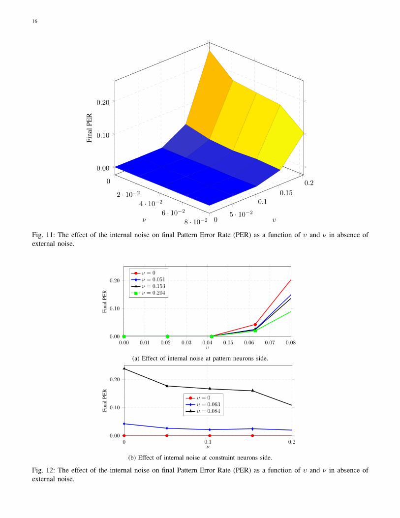
C. Effect of internal noise on the performance in absence of external noise

Now we provide results of a study for a slightly modified setting where there is only internal noise and noexternal errors and further ϕ < υ. Thus, the internal noise can now cause neurons to make wrong decisions, evenin the absence of external errors. With abuse of notation, we assume pattern neurons are corrupted with a ±1 noiseadded to them with probability υ. The rest of the model setting is the same as before.

Figure 11 illustrates the effect of internal noise as a function of υ and ν, the noise parameters at the pattern andconstraint nodes, respectively. This behavior is shown in Figs. 12a and 12b for better inspection. Here, we witnessthe more familiar phenomenon where increasing the amount of internal noise results in a worse performance. This

14

0

0.2

0.40

0.10.2

0.30.4

0.5

0.00

10.00

20.00

30.00

40.00

νυ

Ave

rage

num

bero

fite

ratio

ns

Fig. 9: The effect of internal noise on the number of iterations performed by Algorithm 2, for different values ofυ and ν with ε = 0.125.

finding emphasizes the importance of choosing update threshold ϕ and ψ properly, according to Lemma 1. SeeAppendix C for details on choosing thresholds.

V. DISCUSSION

We have demonstrated that associative memories with exponential capacity still work reliably even when builtfrom unreliable hardware, addressing a major problem in fault-tolerant computing and further arguing for theviability of associative memory models for the (noisy) mammalian brain. After all, brain regions modeled asassociative memories, such as the hippocampus and the olfactory cortex, certainly do display internal noise [18],[21], [46].

The linear-nonlinear computations of Algorithm 1 are nearly identical to message-passing algorithms such asbelief propagation and are certainly biologically plausible [47]–[53]. The state reversion computation of Algorithm 2requires keeping a state variable for a short amount of time which has been suggested as realistic for biologicalneurons [54], but the general biological plausibility of Algorithm 2 remains an open question.

We found a threshold phenomenon for reliable operation, which manifests the tradeoff between the amount ofinternal noise and the amount of external noise that the system can handle. In fact, we showed that internal noiseactually improves the performance of the network in dealing with external errors, up to some optimal value. Thisis a manifestation of the stochastic facilitation [21] or noise enhancement [23] phenomenon that has been observedin other neuronal and signal processing systems, providing a functional benefit to variability in the operation ofneural systems.

The associative memory design developed herein uses thresholding operations in the message-passing algorithmfor recall; as part of our investigation, we optimized these neural firing thresholds based on the statistics of theinternal noise. As noted by Sarpeshkar in describing the properties of analog and digital computing circuits, “Ina cascade of analog stages, noise starts to accumulate. Thus, complex systems with many stages are difficult tobuild. [In digital systems] Round-off error does not accumulate significantly for many computations. Thus, complexsystems with many stages are easy to build” [55]. One key to our result is capturing this benefit of digital processing(thresholding to prevent the build up of errors due to internal noise) as well as a modular architecture which allowsus to correct a linear number of external errors (in terms of the pattern length).

15

0 0.1 0.2 0.3 0.40

10

20

30

40

ν

Ave

rage

num

bero

fite

ratio

ns

υ = 0υ = 0.1υ = 0.2υ = 0.3

(a) Effect of internal noise at constraint neurons side.

0 0.1 0.2 0.3 0.40

10

20

30

40

υ

Ave

rage

num

bero

fite

ratio

ns ν = 0ν = 0.2ν = 0.3ν = 0.5

(b) Effect of internal noise at pattern neurons side.

Fig. 10: The effect of internal noise on the number of iterations performed by Algorithm 2, for different values ofυ and ν with ε = 0.125. The average iteration number of 40 indicate the failure of Algorithm 2.

This paper focused on recall, however learning is the other critical stage of associative memory operation. Indeed,information storage in nervous systems is said to be subject to storage (or learning) noise, in situ noise, and retrieval(or recall) noise [17, Figure 1]. It should be noted, however, there is no essential loss by combining learning noiseand in situ noise into what we have called external error herein, cf. [43, Fn. 1 and Prop. 1]. Thus our basic qualitativeresult extends to the setting where the learning and stored phases are also performed with noisy hardware.

Going forward, it is of interest to investigate other neural information processing models that explicitly incorporateinternal noise and see whether they provide insight into observed empirical phenomena. As an example, we mightbe able to explain the threshold phenomenon observed in the symbol error rate of human telegraph operators underheat stress [56, Figure 2], by invoking a thermal internal noise explanation. Returning to engineering, internal noisein decoders for limited-length error-correcting codes may improve performance as observed herein, since stoppingsets are a limiting phenomenon in that setting also.

ACKNOWLEDGMENT

We thank S. S. Venkatesh for telling us about [15].

APPENDIX AILLUSTRATING PROOF OF THEOREM 2

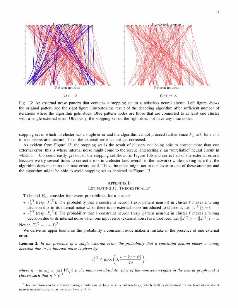
Figure 13a illustrates an example of a stopping set over the graph G in our empirical studies. In the figure,only the nodes corrupted with external noise are shown for clarity. Pattern neurons that are connected to at leastone cluster with a single error are colored blue and other pattern neurons are colored red. Figure 13b illustratesthe same network but after a number of decoding iterations that result in the algorithm getting stuck. We have a

16

0

2 · 10−2

4 · 10−2

6 · 10−2

8 · 10−2 05 · 10−2

0.10.15

0.2

0.00

0.10

0.20

ν υ

Fina

lPE

R

Fig. 11: The effect of the internal noise on final Pattern Error Rate (PER) as a function of υ and ν in absence ofexternal noise.

0.00 0.01 0.02 0.03 0.04 0.05 0.06 0.07 0.080.00

0.10

0.20

υ

Fina

lPE

R

ν = 0ν = 0.051ν = 0.153ν = 0.204

(a) Effect of internal noise at pattern neurons side.

0 0.1 0.20.00

0.10

0.20

ν

Fina

lPE

R

υ = 0υ = 0.063υ = 0.084

(b) Effect of internal noise at constraint neurons side.

Fig. 12: The effect of the internal noise on final Pattern Error Rate (PER) as a function of υ and ν in absence ofexternal noise.

17

0 200 400 600 800 1000 1200 1400 1600 1800 20000

0.5

1

1.5

2

2.5

3

3.5

4

4.5

5

Pattern neurons

Constraint neurons

(a) t = 0

0 200 400 600 800 1000 1200 1400 1600 1800 20000

0.5

1

1.5

2

2.5

3

3.5

4

4.5

5

Pattern neurons

Constraint neurons

(b) t→∞

Fig. 13: An external noise pattern that contains a stopping set in a noiseless neural circuit. Left figure showsthe original pattern and the right figure illustrates the result of the decoding algorithm after sufficient number ofiterations where the algorithm gets stuck. Blue pattern nodes are those that are connected to at least one clusterwith a single external error. Obviously, the stopping set on the right does not have any blue nodes.

stopping set in which no cluster has a single error and the algorithm cannot proceed further since Pci ' 0 for i > 1in a noiseless architecture. Thus, the external error cannot get corrected.

As evident from Figure 13, the stopping set is the result of clusters not being able to correct more than oneexternal error; this is where internal noise might come to the rescue. Interestingly, an “unreliable” neural circuit inwhich υ = 0.6 could easily get out of the stopping set shown in Figure 13b and correct all of the external errors.Because we try several times to correct errors in a cluster (and overall in the network) while making sure that thealgorithm does not introduce new errors itself. Thus, the noise might act in our favor in one of these attempts andthe algorithm might be able to avoid stopping set as depicted in Figure 13.

APPENDIX BESTIMATING Pc1 THEORETICALLY

To bound Pc1 , consider four event probabilities for a cluster:

• π(`)0 (resp. P (`)

0 ): The probability that a constraint neuron (resp. pattern neuron) in cluster ` makes a wrongdecision due to its internal noise when there is no external noise introduced to cluster `, i.e. ‖z(`)‖0 = 0.

• π(`)1 (resp. P (`)

1 ): The probability that a constraint neuron (resp. pattern neuron) in cluster ` makes a wrongdecision due to its internal noise when one input error (external noise) is introduced, i.e. ‖z(`)‖0 = ‖z(`)‖1 = 1.

Notice P (`)c1 = 1− P (`)

1 .We derive an upper bound on the probability a constraint node makes a mistake in the presence of one external

error.

Lemma 2. In the presence of a single external error, the probability that a constraint neuron makes a wrongdecision due to its internal noise is given by

π(`)1 ≤ max

(0,ν − (η − ψ)

2ν

),

where η = mini,j,Wij 6=0 (|Wij |) is the minimum absolute value of the non-zero weights in the neural graph and ischosen such that η ≥ ψ.7

7This condition can be enforced during simulations as long as ψ is not too large, which itself is determined by the level of constraintneuron internal noise, ν, as we must have ψ ≥ ν.

18

Proof: Without loss of generality, assume it is the first pattern node, x(`)1 , that is corrupted with noise +1.Now calculate the probability that a constraint node makes a mistake in such circumstances. We only need analyzeconstraint neurons connected to x(`)1 since the situation for other constraint neurons is as when there is no externalerror. For a constraint neuron j connected to x(`)1 , the decision parameter is

h(`)j =

(W (`).(x(`) + z(`))

)j

+ vj

= 0 +(W (`).z(`)

)j

+ vj

= wj1 + vj .

We consider two error events:• A constraint node j makes a mistake and does not send a message at all. The probability of this event is

denoted by π(1)1 .• A constraint node j makes a mistake and sends a message with the opposite sign. The probability of this event

is denoted by π(1)2 .We first calculate the probability of π(1)2 . Without loss of generality, assume the wj1 > 0 so that the probability

of an error of type two is as follows (the case for wj1 < 0 is exactly the same):

π(1)2 = Pr{wji + vj < −ψ} (12)

= max

(0,ν − (ψ + wj1)

2ν

).

However, since ψ > ν and wj1 > 0, then ν − (ψ + wj1) < 0 and π(1)2 = 0. Therefore, the constraint neurons

will never send a message that has an opposite sign to what it should have. All that remains is to calculate theprobability they remain silent by mistake.

To this end, we have

π(1)1 = Pr{|wji + vj | < ψ} (13)

= max

(0,ν + min(ψ − wj1, ν)

2ν

).

This can be simplified if we assume that the absolute values of all weights in the network are bigger than a constantη > ψ. Then, the above equation will simplify to

π(1)1 ≤ max

(0,ν − (η − ψ)

2ν

). (14)

Putting the above equations together, we obtain:

π(1) ≤ max

(0,ν − (η − ψ)

2ν

). (15)

In the case η − ψ > ν, we could even manage to make this probability equal to zero. However, we will leave itas is and use (15) to calculate P (`)

1 .

A. Calculating P (`)1

We start by calculating the probability that a non-corrupted pattern node x(`)j makes a mistake, which is to change

its state in round 1. Let us denote this probability by q(`)1 . Now to calculate q(`)1 assume x(`)j has degree dj and it

has b common neighbors with x(`)1 , the corrupted pattern node.Out of these b common neighbors, bc will send ±1 messages and the others will, mistakenly, send nothing. Thus,

the decision making parameter of pattern node j, g(`)j , will be bounded by

g(`)j =

(sign(W (`))> · y(`)

)j

dj+ uj . ≤

bcdj

+ uj .

19

We denote(sign(W (`))> · y(`)

)j

by oj for brevity from this point on.

In this circumstance, a mistake happens when |g(`)j | ≥ ϕ. Thus

q(`)1 = Pr{|g(`)j | ≥ ϕ|deg(aj) = dj&|N (x1) ∩N (aj)| = a} (16)

= Pr{ojdj

+ uj ≥ ϕ}+ Pr{ojdj

+ uj ≤ −ϕ},

where N (ai) represents the neighborhood of pattern node ai among constraint nodes.By simplifying (16) we get

q(`)1 (oj) =

+1, if |oj | ≥ (υ + ϕ)dj

max(0, υ−ϕυ ), if |oj | ≤ |υ − ϕ|djυ−(ϕ−oj/dj)

2υ , if |oj − ϕdj | ≤ υdjυ−(ϕ+oj/dj)

2υ , if |oj + ϕdj | ≤ υdj .

We now average this equation over oj , bc, b and dj . To start, suppose that out of the bc non-zero messagesnode aj receives, e of them have the same sign as the link they are being transmitted over. Thus, we will haveoj = e − (bc − e) = 2e − bc. Assuming the probability of having the same sign for each message is 1/2, theprobability of having e equal signs out of bc elements will be

(bce

) (12

)bc . Thus, we will get

q(`)1 =

bc∑e=0

(bce

)(1

2

)bcq(`)1 (2e− bc). (17)

Now note that the probability of having a− bc mistakes from the constraint side is given by(bbc

)(π

(`)1 )b−bc(1−

π(`)1 )bc . With some abuse of notations we get:

q(`)1 =

b∑bc=0

(b

bc

)(π

(`)1 )b−bc(1− π(`)1 )bc

bc∑e=0

(bce

)(1

2

)bcq(`)1 (2e− bc). (18)

Finally, the probability that aj and x1 have b common neighbors can be approximated by(djb

)(1−d(`)/m`)

dj−b(d(`)/m`)b,

where d(`) is the average degree of pattern nodes. Thus (again abusing some notation), we obtain:

q(`)1 =

dj∑b=0

pb

b∑bc=0

pbc

bc∑e=0

(bce

)(1

2

)bcq(`)1 (2e− bc), (19)

where q(`)1 (2e − bc) is given by (16), pb is the probability of having b common neighbors and is estimated by(dj

b

)(1− d(`)/m`)

dj−b(d(`)/m`)b, with d(`) being the average degree of pattern nodes in cluster `. Furthermore, pbc

is the probability of having b− bc out of these b nodes making mistakes. Hence, pbc =(bbc

)(π

(`)1 )b−bc(1− π(`)1 )bc .

We will not simplify the above equation any further and use it as it is in our numerical analysis in order to obtainthe best parameter ϕ.

Now we turn our attention to the probability that the corrupted node, x1, makes a mistake, which is either notto update at all or update itself in the wrong direction. Recalling that we have assume the external noise term inx1 to be a +1 noise, the wrong direction would be for node x1 to increase its current value instead of decreasingit. Furthermore, we assume that out of d1 neighbors of x1, some j of them have made a mistake and will not sendany messages to x1. Thus, the decision parameter of x1, will be g(`)1 = u+ (d1 − j)/d1. Denoting the probabilityof making a mistake at x1 by q(`)2 we get:

q(`)2 = Pr{g(`)1 ≤ ϕ|deg(x1) = d1 and j errors in constraints} (20)

= Pr{d1 − jd1

+ u < ϕ

},

20

0.00 0.20 0.40 0.60 0.80 1.000.00

0.20

0.40

0.60

0.80

1.00

ϕ

P(ℓ)

1

υ = 0.1υ = 0.2υ = 0.4υ = 0.95

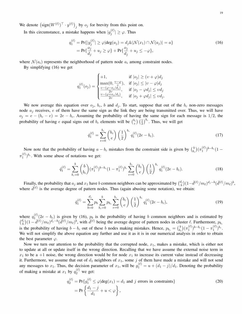
Fig. 14: The behavior of Pc1 as a function of ϕ for different values of noise parameter, υ. Here, π(1) = 0.01.

which simplifies to

q(`)2 (j) =

+1, if |j| ≥ (1 + υ − ϕ)d1

max(0, υ−ϕυ ), if |j| ≤ (1− υ − ϕ)d1υ+ϕ−(d1−j)/d1

2υ , if |ϕd1 − (d1 − j)| ≤ υd1.

(21)

Noting that the probability of making j mistakes on the constraint side is(d1j

)(π

(`)1 )j(1− π(`)1 )d1−j , we get

q(`)2 =

d1∑j=0

(d1j

)(π

(`)1 )j(1− π(`)1 )d1−jq

(`)2 (j), (22)

where q(`)2 (j) is given by (21).Putting the above results together, the overall probability of making a mistake on the side of pattern neurons

when we have one bit of external noise is

P(`)1 =

1

n(`)q(`)2 +

n(`) − 1

n(`)q(`)1 . (23)

Finally, the probability that cluster ` could correct one error is that all neurons take the correct decision, i.e.

P (`)c1 = (1− P (`)

1 )n(`)

and the average probability that clusters could correct one error is simply

Pc1 = E`(P (`)c1 ). (24)

We use this equation in order to find the best update threshold ϕ.

APPENDIX CCHOOSING PROPER ϕ

We now apply numerical methods to (23) to find the best ϕ for different values of noise parameter υ. Thefollowing figures show the best choice for the parameter ϕ. The update threshold on the constraint side is chosensuch that ψ > ν. In each figure, we have illustrated the final probability of making a mistake, P (`)

1 , for comparison.

Figure 14 illustrates the behavior of the average probability of correcting a single error, Pc1 , as a function of ϕfor different values of υ and for π1 = 0.01. The interesting trend here is that in all cases, ϕ∗, the update threshold

21

0.00 0.20 0.40 0.60 0.80 1.000.70

0.80

0.90

υ

ϕ∗

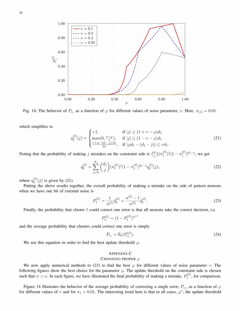
Fig. 15: The behavior of ϕ∗ as a function of υ for π1 = 0.01.

0.00 0.50 1.000.00

0.50

1.00

υ

P(ℓ)

1

π1 = 0π1 = 0.01π1 = 0.1

Fig. 16: The optimum Pe1 as a function of υ for different values π1.

that gives the best result, is chosen such that it is quite large. This actually is in line with our expectation because asmall ϕ will result in non-corrupted nodes to update their states more frequently. On the other hand, a very large ϕwill prevent the corrupted nodes to correct their states, especially if there are some mistakes made on the constraintside, i.e., π(`)1 > 0. Therefore, since we have much more non-corrupted nodes than corrupted nodes, it is best tochoose a rather high ϕ but not too high. Please also note that when π(`)1 is very high, there are no values of υ forwhich error-free storage is possible.

Figure 15 illustrates the exact behavior of ϕ∗ against υ for the case where φ1 = 0. As can be seen from thefigure, ϕ should be quite large.

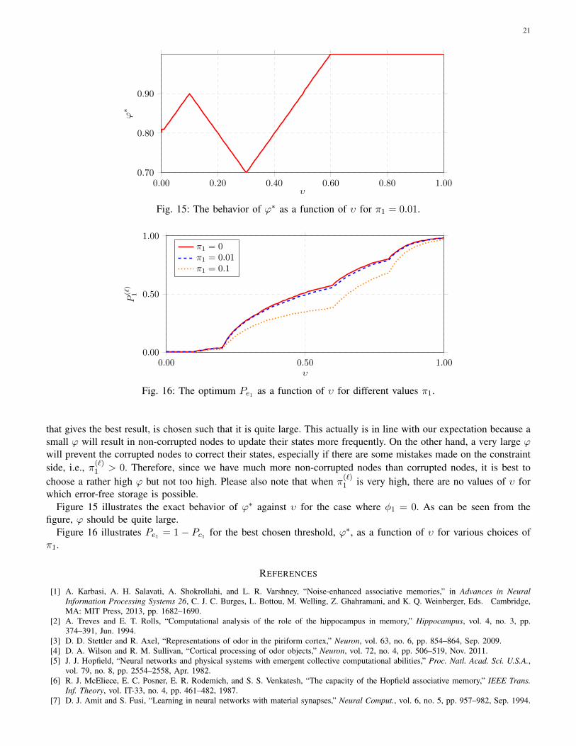
Figure 16 illustrates Pe1 = 1− Pc1 for the best chosen threshold, ϕ∗, as a function of υ for various choices ofπ1.

REFERENCES

[1] A. Karbasi, A. H. Salavati, A. Shokrollahi, and L. R. Varshney, “Noise-enhanced associative memories,” in Advances in NeuralInformation Processing Systems 26, C. J. C. Burges, L. Bottou, M. Welling, Z. Ghahramani, and K. Q. Weinberger, Eds. Cambridge,MA: MIT Press, 2013, pp. 1682–1690.

[2] A. Treves and E. T. Rolls, “Computational analysis of the role of the hippocampus in memory,” Hippocampus, vol. 4, no. 3, pp.374–391, Jun. 1994.

[3] D. D. Stettler and R. Axel, “Representations of odor in the piriform cortex,” Neuron, vol. 63, no. 6, pp. 854–864, Sep. 2009.[4] D. A. Wilson and R. M. Sullivan, “Cortical processing of odor objects,” Neuron, vol. 72, no. 4, pp. 506–519, Nov. 2011.[5] J. J. Hopfield, “Neural networks and physical systems with emergent collective computational abilities,” Proc. Natl. Acad. Sci. U.S.A.,

vol. 79, no. 8, pp. 2554–2558, Apr. 1982.[6] R. J. McEliece, E. C. Posner, E. R. Rodemich, and S. S. Venkatesh, “The capacity of the Hopfield associative memory,” IEEE Trans.

Inf. Theory, vol. IT-33, no. 4, pp. 461–482, 1987.[7] D. J. Amit and S. Fusi, “Learning in neural networks with material synapses,” Neural Comput., vol. 6, no. 5, pp. 957–982, Sep. 1994.

22

[8] G. Palm, “On associative memory,” Biol. Cybern., vol. 36, no. 1, pp. 19–31, Feb. 1980.[9] C. E. Shannon, “A mathematical theory of communication,” Bell Syst. Tech. J., vol. 27, pp. 379–423, 623–656, July/Oct. 1948.

[10] B. A. Olshausen and D. J. Field, “Sparse coding of sensory inputs,” Curr. Opin. Neurobiol., vol. 14, no. 4, pp. 481–487, Aug. 2004.[11] A. A. Koulakov and D. Rinberg, “Sparse incomplete representations: A potential role of olfactory granule cells,” Neuron, vol. 72, no. 1,

pp. 124–136, Oct. 2011.[12] T. Richardson and R. Urbanke, Modern Coding Theory. Cambridge: Cambridge University Press, 2008.[13] A. H. Salavati and A. Karbasi, “Multi-level error-resilient neural networks,” in Proc. 2012 IEEE Int. Symp. Inf. Theory, Jul. 2012, pp.

1064–1068.[14] A. Karbasi, A. H. Salavati, and A. Shokrollahi, “Iterative learning and denoising in convolutional neural associative memories,” in

Proc. 30th Int. Conf. Mach. Learn. (ICML 2013), Jun. 2013, to appear.[15] S. Biswas, “A performance analysis of sparse neural associative memory,” Ph.D. dissertation, University of Pennsylvania, 1993.[16] N. Brunel, V. Hakim, P. Isope, J.-P. Nadal, and B. Barbour, “Optimal information storage and the distribution of synaptic weights:

Perceptron versus Purkinje cell,” Neuron, vol. 43, no. 5, pp. 745–757, 2004.[17] L. R. Varshney, P. J. Sjostrom, and D. B. Chklovskii, “Optimal information storage in noisy synapses under resource constraints,”

Neuron, vol. 52, no. 3, pp. 409–423, Nov. 2006.[18] C. Koch, Biophysics of Computation: Information Processing in Single Neurons. New York: Oxford University Press, 1999.[19] A. A. Faisal, L. P. J. Selen, and D. M. Wolpert, “Noise in the nervous system,” Nat. Rev. Neurosci., vol. 9, no. 4, pp. 292–303, Apr.

2008.[20] E. T. Rolls and G. Deco, The Noisy Brain: Stochastic Dynamics as a Principle of Brain Function. Oxford University Press, 2010.[21] M. D. McDonnell and L. M. Ward, “The benefits of noise in neural systems: bridging theory and experiment,” Nat. Rev. Neurosci.,

vol. 12, no. 7, pp. 415–426, Jul. 2011.[22] A. Destexhe and M. Rudolph-Lilith, Neuronal Noise. New York: Springer, 2012.[23] H. Chen, P. K. Varshney, S. M. Kay, and J. H. Michels, “Theory of the stochastic resonance effect in signal detection: Part I–fixed

detectors,” IEEE Trans. Signal Process., vol. 55, no. 7, pp. 3172–3184, Jul. 2007.[24] D. A. Spielman and S.-H. Teng, “Smoothed analysis of algorithms: Why the simplex algorithm usually takes polynomial time,” J.

ACM, vol. 51, no. 3, pp. 385–463, May 2004.[25] D. O. Hebb, The Organization of Behavior: A Neuropsychological Theory. New York: Wiley, 1949.[26] S. Jankowski, A. Lozowski, and J. M. Zurada, “Complex-valued multistate neural associative memory,” IEEE Trans. Neural Netw.,

vol. 7, no. 6, pp. 1491–1496, Nov. 1996.[27] M. K. Muezzinoglu, C. Guzelis, and J. M. Zurada, “A new design method for the complex-valued multistate Hopfield associative

memory,” IEEE Trans. Neural Netw., vol. 14, no. 4, pp. 891–899, Jul. 2003.[28] D.-L. Lee, “Improvements of complex-valued Hopfield associative memory by using generalized projection rules,” IEEE Trans. Neural

Netw., vol. 17, no. 5, pp. 1341–1347, Sep. 2006.[29] V. Gripon and C. Berrou, “Sparse neural networks with large learning diversity,” IEEE Trans. Neural Netw., vol. 22, no. 7, pp.

1087–1096, Jul. 2011.[30] S. S. Venkatesh, “Connectivity versus capacity in the Hebb rule,” in Theoretical Advances in Neural Computation and Learning,

V. Roychowdhury, K.-Y. Siu, and A. Orlitsky, Eds. Kluwer Academic Publishers, 1994, pp. 173–240.[31] Y. Baram, “Encoding unique global minima in nested neural networks,” IEEE Trans. Inf. Theory, vol. 37, no. 4, pp. 1158–1162, Jul.

1991.[32] P. Peretto and J. J. Niez, “Long term memory storage capacity of multiconnected neural networks,” Biol. Cybern., vol. 54, no. 1, pp.

53–63, May 1986.[33] L. Xu, A. Krzyzak, and E. Oja, “Neural nets for dual subspace pattern recognition method,” Int. J. Neur. Syst., vol. 2, no. 3, pp.

169–184, 1991.[34] E. J. Candes and T. Tao, “Near-optimal signal recovery from random projections: Universal encoding strategies?” IEEE Trans. Inf.

Theory, vol. 52, no. 12, pp. 5406–5425, Dec. 2006.[35] A. K. Fletcher, S. Rangan, L. R. Varshney, and A. Bhargava, “Neural reconstruction with approximate message passing (NeuRAMP),”

in Advances in Neural Information Processing Systems 24, J. Shawe-Taylor, R. Zemel, P. Bartlett, F. Pereira, and K. Weinberger, Eds.Cambridge, MA: MIT Press, 2011, pp. 2555–2563.

[36] P. Vincent, H. Larochelle, Y. Bengio, and P.-A. Manzagol, “Extracting and composing robust features with denoising autoencoders,”in Proc. 25th Int. Conf. Mach. Learn. (ICML 2008), Jul. 2008, pp. 1096–1103.

[37] Q. V. Le, J. Ngiam, Z. Chen, D. Chia, P. W. Koh, and A. Y. Ng, “Tiled convolutional neural networks,” in Advances in NeuralInformation Processing Systems 23, J. Lafferty, C. K. I. Williams, J. Shawe-Taylor, R. S. Zemel, and A. Culotta, Eds. Cambridge,MA: MIT Press, 2010, pp. 1279–1287.

[38] S. Song, P. J. Sjostrom, M. Reigl, S. Nelson, and D. B. Chklovskii, “Highly nonrandom features of synaptic connectivity in localcortical circuits,” PLoS Biol., vol. 3, no. 3, pp. 0507–0519, Mar. 2005.

[39] D. J. Amit, Modeling Brain Function. Cambridge: Cambridge University Press, 1992.[40] H. Liljenstrom and X.-B. Wu, “Noise-enhanced performance in a cortical associative memory model,” Int. J. Neur. Syst., vol. 6, no. 1,

pp. 19–29, Mar. 1995.[41] M. G. Taylor, “Reliable information storage in memories designed from unreliable components,” Bell Syst. Tech. J., vol. 47, no. 10,

pp. 2299–2337, Dec. 1968.[42] A. V. Kuznetsov, “Information storage in a memory assembled from unreliable components,” Probl. Inf. Transm., vol. 9, no. 3, pp.

100–114, July-Sept. 1973.[43] L. R. Varshney, “Performance of LDPC codes under faulty iterative decoding,” IEEE Trans. Inf. Theory, vol. 57, no. 7, pp. 4427–4444,

Jul. 2011.[44] M. G. Luby, M. Mitzenmacher, M. A. Shokrollahi, and D. A. Spielman, “Efficient erasure correcting codes,” IEEE Trans. Inf. Theory,

vol. 47, no. 2, pp. 569–584, Feb. 2001.

23

[45] S. M. S. Tabatabaei Yazdi, H. Cho, and L. Dolecek, “Gallager B decoder on noisy hardware,” IEEE Trans. Commun., vol. 61, no. 5,pp. 1660–1673, May 2013.

[46] M. Yoshida, H. Hayashi, K. Tateno, and S. Ishizuka, “Stochastic resonance in the hippocampal CA3–CA1 model: a possible memoryrecall mechanism,” Neural Netw., vol. 15, no. 10, pp. 1171–1183, Dec. 2002.

[47] J. M. Beck and A. Pouget, “Exact inferences in a neural implementation of a hidden Markov model,” Neural Comput., vol. 19, no. 5,pp. 1344–1361, May 2007.

[48] P. Dayan, G. E. Hinton, R. M. Neal, and R. S. Zemel, “The Helmholtz machine,” Neural Comput., vol. 7, no. 5, pp. 889–904, Sep.1995.

[49] S. Deneve, “Bayesian spiking neurons I: Inference,” Neural Comput., vol. 20, no. 1, pp. 91–117, Jan. 2008.[50] K. Doya, S. Ishii, A. Pouget, and R. P. N. Rao, Bayesian Brain: Probabilistic Approaches to Neural Coding. Cambridge, MA: MIT

Press, 2007.[51] G. E. Hinton and T. J. Sejnowski, “Learning and relearning in Boltzmann machines,” in Parallel Distributed Processing: Explorations

in the Microfoundations of Cognition, Volume 1: Foundations, D. E. Rumelhart and J. L. McLelland, Eds. Cambridge, MA: MITPress, 1986, pp. 282–317.

[52] W. J. Ma, J. M. Beck, P. E. Latham, and A. Pouget, “Bayesian inference with probabilistic population codes,” Nat. Neurosci., vol. 9,no. 11, pp. 1432–1438, Nov. 2006.

[53] S. Litvak and S. Ullman, “Cortical circuitry implementing graphical models,” Neural Comput., vol. 21, no. 11, pp. 3010–3056, Nov.2009.

[54] S. Druckmann and D. B. Chklovskii, “Neuronal circuits underlying persistent representations despite time varying activity,” Curr. Biol.,vol. 22, no. 22, pp. 2095–2103, Oct. 2012.

[55] R. Sarpeshkar, “Analog versus digital: Extrapolating from electronics to neurobiology,” Neural Comput., vol. 10, no. 7, pp. 1601–1638,Oct. 1998.

[56] N. H. Mackworth, “Effects of heat on wireless telegraphy operators hearing and recording Morse messages,” Br. J. Ind. Med., vol. 3,no. 3, pp. 143–158, Jul. 1946.