In" Kosko, B., NEURAL NETWORKS AND FUZZY SYSTEMS, Prentice-Hall, 1990

N91-21779

CHAPTER 17

FUZZY ASSOCIATIVE MEMORIES-

Fuzzy Systems as Between-Cube Mappings

In Chapter 16, we introdnced continuous or fuzzy sets as points in the unit hypercube

I" = [0, 1] ". Within the cube we were interested in the distance between points. This led

to measures of the size and fuzziness of a fuzzy set and, more fundamentally, to a measure

of how much one fuzzy set is a subset of another fuzzy set. This within-cube theory directly

extends to the continuous case where the space X is a subset of R '_ or, in general, where

X is a subset of products of real or complex spaces.

The next step is to consider mappings between fuzzy cubes. This level of abstraction

provides a s.urprising and fruitful alternative to the propositional and predicate-calculus

reasoning techniques used in artificial-intelligence (AI) expert systems. It allows us to

reason with sets instead of propositions.

The fuzzy set framework is numerical and multidimensional. The AI framework is

symbolic and one-dimensional, with usually only bivalent expert "rules" or propositions

allowed. Both frameworks can encode structured knowledge in linguistic t'orm. But the

fuzzy approach translates the structured knowledge into a flexible numerical framework

and processes it in a manner that resembles neural network processing. The numerical

framework also allows fuzzy systems to be adal)tively inferred and modified, perhal)s with

neural or statistical tech.iques, directly fi'om problem domain sample data.

https://ntrs.nasa.gov/search.jsp?R=19910012466 2018-08-07T13:46:32+00:00Z

Between-cube theory is fuzzy systems theory. A fuzzy set is a point in a cube. A

fuzzy system is a mapping between cubes. A fuzzy system S maps fuzzy sets to fuzzy

sets. Thus a fuzzy system S is a transformation S : I n ---* i p. The n-dimensional

unit hypercube I '_ houses all the fuzzy subsets of the domain space, or input universe of

discourse, X = {xl,..., x,}. I p houses all the fuzzy subsets of the range space, or output

universe of discourse, Y = {Yl,..., Yp}. X and Y can also be subsets of R" and R p. Then

the fuzzy power sets F(2 x) and F(2 Y) replace I" and I p.

In general a fuzzy system S maps families of fuzzy sets to families of fuzzy sets, thus

S : I m x... x I "r ---* I p_ x...x I p°. Here too we can extend the definition of a

fuzzy system to allow arbitrary products of arbitrary mathematical spaces to serve as the

domain or range spaces of the fuzzy sets.

(A technical comment is in order for sake of historical clarification. A tenet, perhaps

the defining tenet, of the classical theory [Dubois, 1980] of fuzzy sets as functions concerns

the fuzzy extension of any mathematical function. This tenet holds that any function

f : X _ Y that maps points inX to points in Y can be extended to map the fuzzy

subsets of X to the fuzzy subsets of Y. The so-called extension principle is used to define

the set-function f : F(2 x) _ F(2Y), where F(2 x) is the fuzzy power set of X, the set

of all fuzzy subsets of X. The formal definition of the extension principle is complicated.

The key idea is a supremum of pairwise minima. Unfortunately, the extension principle

achieves generality at the price of triviality. One can show [Kosko, 1986a-87] that in general

the extension principle extends functions to fuzzy sets by stripping the fuzzy sets of their

fuzziness, mapping the fuzzy sets into bit vectors of nearly all ls. This shortcoming,

combined with the tendency of the extension-principle framework to push fuzzy theory

into largely inaccessible regions of abstract mathematics, led in part to the development

of the alternative sets-as-points geometric framework of fuzzy theory.)

We shall focus on fuzzy systems S : I n ---* I p that map balls of fuzzy sets in ] n to

balls of fuzzy sets in I p. These continuous fuzzy systems behave as associative memories.

They map close inputs to close outputs. We shall refer to them as fuzzy associative

memories, or FAMs.

The simplest FAM encodes the FAM rule or association (Ai, Bi), which associates

4

the p-dimensional fuzzy set Bi with the n-dimensional fuzzy set Ai. These minimal FAMs

essentially map one bah in I n to one ball in I p. They are comparable to simple neura]

networks. But the minimal FAMs need not be adaptively trained. As discussed below,

structured knowledge of the form "If traffic is heavy in this direction, then keep the stop

light green longer" can be directly encoded in a Hebbian-style FAM matrix. In practice

we can eliminate even this matrix. In its place the user encodes the fuzzy-set association

(HEAVY, LONGER) as a single linguistic entry in a FAM bank matrix.

In general a FAM system F : I" _ I p encodes and processes in parallel _ FAM

bank of m FAM rules (A1, B1),..., (Am, B,,,). Each input A to the FAM system activates

each stored FAM rule to different degree. The minimal FAM that stores (Ai,/3,.) maps

input A to B_, a partially activated version of Bi. The more A resembles Ai, the more B[

resembles Bi. The corresponding output fuzzy set B combines these partially activated

fuzzy sets B_,..., B_. In the simplest case B is a weighted average of the partially activated

sets:

B = wlB_ + ... + w,,, B',,, ,

where wi reflects the credibility, frequency, or strength of the fuzzy association (Ai, Bi). In

practice we usually "defuzzify" the output waveform B to a single numerical value b'j in Y

by computing the fuzzy centroid of B with respect to the output universe of discourse Y.

More general still, a FAM system encodes a bank of compound FAM rules that associate

multiple output or consequent fuzzy sets B_,..., B_' with multiple input or antecedent fuzzy

sets A_,... ,At. We can treat compound FAM rules as compound linguistic conditionals.

Structured knowledge can then be naturally, and in many cases easily, obtained. We

combine antecedent and consequent sets with logical conjunction, disjunction, or negation.

For instance, we would interpret the compound association (A a, A2; B) linguistically as

the compound conditional "IF X a is A 1 AND X 7 is A 2 , THEN Y is B" if the comma in

the fuzzy association (A 1, A2; B) stood for conjunction instead of, say, disjunction.

We specify in advance the numerical universes of discourse X 1, X _, and Y. For each

universe of discourse X, we specify an appropriate library of fuzzy set values, A_,..., A_.

Contiguous fuzzy sets in a library overlap. In principle a neural network can estimate these

5

libraries of fuzzy sets. In practice this is usually unnecessary.The library sets represent

a weighted, though overlapping, quantization of the input space X. A different library of

fuzzy sets similarly quantizes the output space Y. Once the library of fuzzy sets is defined,

we construct the FAM by choosing appropriate combinations of input and output fuzzy

sets. We can use adaptive techniques to make, assist, or modify these choices.

An adaptive FAM (AFAM) is a time-varying FAM system. System parameters grad-

ually change as the FAM system samples and processes data. Below we discuss how neural

network algorithms can adaptively infer FAM rules from training data. In principle learn-

ing can modify other FAM system components, such as the libraries of fuzzy sets or the

FAM-rule weights wi.

Below we propose and illustrate an unsupervised adaptive clustering scheme, based on

competitive learning, for "blindly" generating and refining the bank of FAM rules. In some

cases we can use supervised learning techniques, though we need additional information

to accurately generate error estimates.

FUZZY AND NEURAL FUNCTION ESTIMATORS

Neural and fuzzy systems estimate sampled functions and behave as associative mem-

ories. They share a key advantage over traditional statistical-estimation and adaptive-

control approaches to function estimation. They are model-free estimators. Neural and

fuzzy systems estimate a function without requiring a mathematical description of how the

output functionally depends on the input. They "learn from example." More precisely,

they learn from samples.

Both approaches are numerical, can be partially described with theorems, and admit an

algorithmic characterization that favors silicon and optical implementation. These prop-

erties distinguish neural and fuzzy approaches from the symbolic processing approaches of

artificial intelligence.

Neural and fuzzy systems differ in how they estimate sampled functions. They differ

in the kind of samples used, how they represent and store those samples, and how they

6

associatively"inference" or map inputs to outputs.

These differencesappear during system construction. The neural approach requires

the specification of a nonlinear dynamical system,usually feedforward, the acquisition of

a sufficiently representativeset of numerical training samples,and the encodingof those

training samplesin the dynamical systemby repeated learning cycles. The fuzzy system

requiresonly that a linguistic "rule matrix" be partially filled in. This task is markedly

simpler than designingand training a neural network. Onceweconstruct the systems,we

can present the samenumerical inputs to either system. The outputs will be in the same

numerical spaceof alternatives. So both systemscorrespondto a surfaceor manifold in

the input-output product spaceX × Y. We present examples of these surfaces in Chapters

18 and 19.

Which system, neural or fuzzy, is more appropriate for a particular problem depends on

the nature of the problem and the availability of numerical and structured data. To date

fuzzy techniques have been most successfully applied to control problems. These problems

often permit comparison with standard control-theoretic and expert-system approaches.

Neural networks so far seem best applied to ill-defined two-class pattern recognition prob-

lems (defective or nondefective, bomb or not, etc.). The application of both approaches to

new problem areas is just beginning, amid varying amounts of enthusiasm and scepticism.

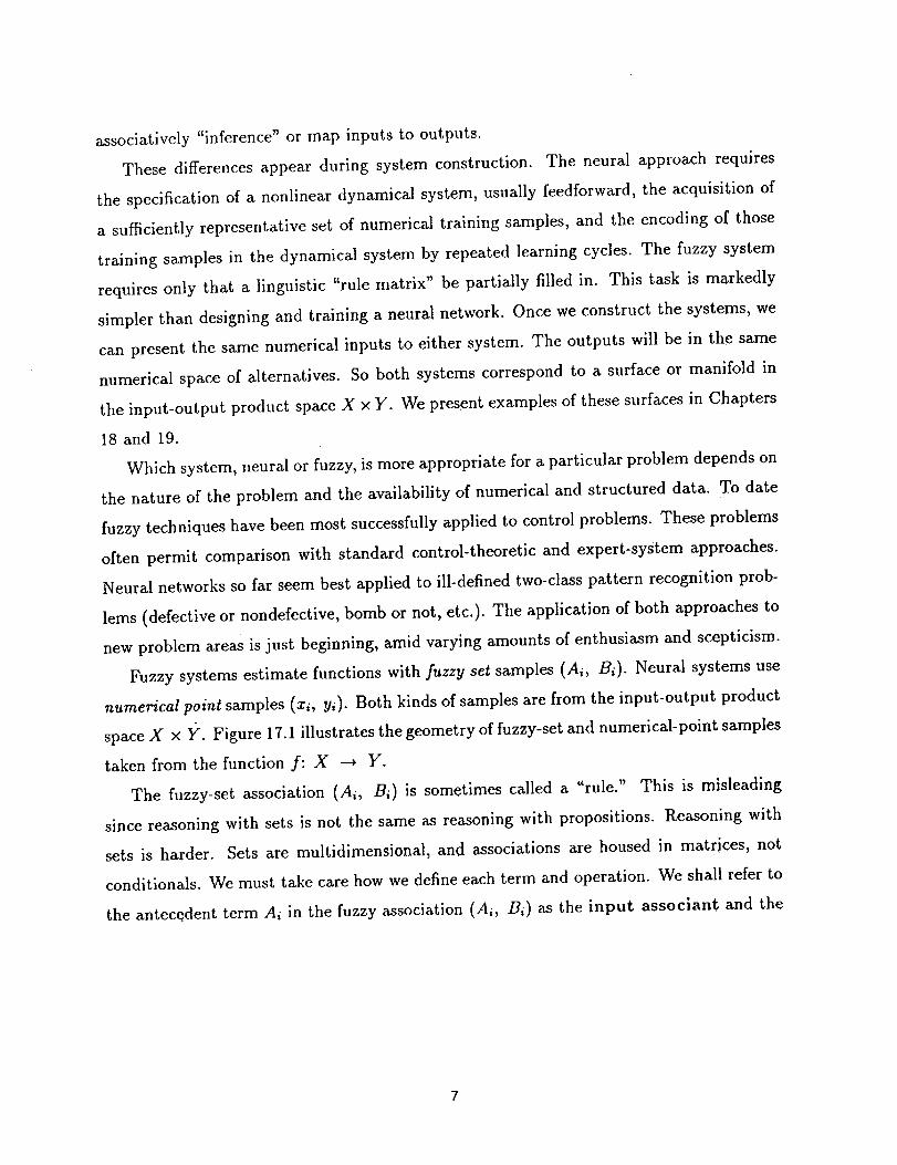
Fuzzy systems estimate functions with fuzzy set samples (Ai, Bi). Neural systems use

numerical point samples (xi, yi). Both kinds of samples are from the input-output product

space X × Y. Figure 17.1 illustrates the geometry of fuzzy-set and numerical-point samples

taken from the function f: X _ Y.

The fuzzy-set association (Ai, Bi) is sometimes called a "rule." This is misleading

since reasoning with sets is not the same as reasoning with propositions. Reasoning with

sets is harder. Sets are multidimensional, and associations are housed in matrices, not

conditionals. We must take care how we define each term and operation. We shall refer to

the antecedent term Ai in the fuzzy association (Ai, Bi) as the input associant and the

consequent term Bi as the output associant.

FIGURE 17.1 Function f maps domain X to range Y. In the first illustra-

tion we use several numerical point samples (xi, yi) to estimate f: X _ Y.

In the second case we use only a few fuzzy subsets Ai of X and Bi of Y. The

fuzzy association (Ai, Bi) represents system structure, as an adaptive cluster-

ing algorithm might infer or as an expert might articulate. In practice there are

usually fewer different output associants or "rule" consequents Bi than input

associants or antecedents Ai.

The fuzzy-set sample (Ai, Bi) encodes structure. It represents a mapping itself, a min-

imal fuzzy association of part of the output space with part of the input space. In practice

this resembles a meta-rule---IF Ai, THEN Bi--the type of structured linguistic rule an ex-

pert might articulate to build an expert-system "knowledge base". The association might

also be the result of an adaptive clustering algorithm.

Consider a fuzzy association that might be used in the intelligent control of a traffic

light: "If the traffic is heavy in this direction, then keep the light green longer." The

fuzzy association is (HEAVY, LONGER). Another fuzzy association might be (LIGHT,

SHORTER). The fuzzy system encodes each linguistic association or "rule" in a numerical

fuzzy associative memory (FAM) mapping. The FAM then numerically processes numerical

input data. A measured description of traffic density (e.g., 150 cars per unit road surface

area) then corresponds to a unique numerical output (e.g., 3 seconds), the "recalled"

output.

The degree to which a particular measurement of traffic density is heavy depends on

how we define the fuzzy set of heavy traffic. The definition may be obtained from statistical

or neural clustering of historical data or from pooling the responses of experts. In practice

the fuzzy engineer and the problem domain expert agree on one of many possible libraries

of fuzzy set definitions for the variables in question.

The degree to which the traffic light is kept green longer depends on the degree to

which the measurement is heavy. In the simplest case the two degrees are the same. In

general they differ. In actual fuzzy systems the output control variables--in this case the

single variable green light duration--depend on many FAM rule antecedents or associants

that are activated to different degrees by incoming data.

9

Neural vs. Fuzzy Representation of Structured Knowledge

The functional distinction between how fuzzy and neural systems differ begins with

how they represent structured knowledge. How would a neural network encode the same

associative information? How would a neural network encode the structured knowledge

"If the traffic is heavy in this direction, then keep the light green longer"?

The simplest method is to encode two associated numerical vectors. One vector rep-

resents the input associant HEAVY. The other vector represents the output associant

LONGER. But this is too simple. For the neural network's fault tolerance now works

to its disadvantage. The network tends to reconstruct partial inputs to complete sample

inputs. It erases the desired partial degrees of activation. If an input is close to Ai, the

output will tend to be Bi. If the output is distant from Ai, the output will tend to be some

other sampled output vector or a spurious output altogether.

A better neural approach is to encode a mapping from the heavy-traffic subspace to

the longer-time subspace. Then the neural network needs a representative sample set to

capture this structure. Statistical networks, such as adaptive vector quantizers, may need

thousands of statistically representative samples. Feedforward multi-layer neural networks

trained with the backpropagation algorithm may need hundreds of representative numerical

input-output pairs and may need to recycle these samples tens of thousands of times in

the learning process.

The neural approach suffers a deeper problem than just the computational burden of

training. What does it encode? How do we know the network encodes the original struc-

ture? What does it recall? There is no natural inferential audit trail. System nonlinearities

wash it away. Unlike an expert system, we do not know which inferential paths the network

uses to reach a given output or even which inferential paths exist. There is only a system of

synchronous or asynchronous nonlinear functions. Unlike, say, the adaptive Kalman filter,

we cannot appeal to a postulated mathematical model of how the output state depends on

the input state. Model-free estimation is, after all, the central computational advantage

of neural networks. The cost is system inscrutability.

10

We are left with anunstructured computational black box. We do not know what the

neural network encodedduring training or what it will encodeor forget in further training.

(For competitive adaptive vector quantizerswe do know that sample-spacecentroids are

asymptotically estimated,) We can characterizethe neural network's behavior only by

exhaustively passingall inputs through the black box and recording the recalled 6utputs.

The characterization may be in terms of a summary scalar like mean-squared error,

This black-box characterization of the network's behavior involves a computational

dilemma. On the one hand, for most problems the number of input-output cases we need

to check is computationally prohibitive. On the other, when the number of input-output

cases is tractable, we may as well store these pairs and appeal to them directly, and without

error, as a look-up table. In the first case the neural network is unreliable. In the second

case it is unnecessary.

A further problem is sample generation. Where did the original numerical point samples

come from? Was an expert asked to give numbers? How reliable are such numerical vectors,

especially when the expert feels most comfortable giving the original linguistic data? This

procedure seems at most as reliable as the expert-system method of asking an expert to

give condition-action rules with numerical uncertainty weights.

Statistical neural estimators require a "statistically representative" sample set. We may

need to randomly "create" these samples from an initial small sample set by bootstrap tech-

niques or by random-number generation of points clustered near the original samples. Both

sample-augmentation procedures assume that the initial sample set sufficiently represents

the underlying probability distribution. The problem of where the original sample set

comes from remains. The fuzziness of the notion "statistically representative" compounds

the problem. In general we do not know in advance how well a given sample set reflects an

unknown underlying distribution of points. Indeed when the network is adapting on-line,

we know only past samples. The remainder of the sample set is in the unsampled future.

In contrast, fuzzy systems directly encode the linguistic sample (HEAVY, LONGER) in

a dedicated numerical matrix. The default encoding technique is the fuzzy Hebb procedure

discussed below. For practical problems, as mentioned above, the numerical matrix need

not be stored. Indeed it need not even be formed. Certain numerical inputs permit this

11

simplification, as we shall seebelow. In general we describe inputs by an uncertainty

distribution, probabilistic or fuzzy. Then we must usethe entire matrix.

For instance, if a heavy traffic input is simply the number 150, we can omit the FAM

matrix. But if the input is a Gaussian curve with mean 150, then in principle we must

process the vector input with a FAM matrix. (In practice we might use only the mean.)

This difference is explained below. The dimensions of the linguistic FAM bank matrix

are usually small. The dimensions reflect the quantization levels of the input and output

spaces.

The fuzzy approach combines the purely numerical approaches of neural networks and

mathematical modeling with the symbolic, structure-rich approaches of artificial intelli-

gence. We acquire knowledge symbolically--or numerically if we use adaptive techniques

--but represent it numerically. We also process data numerically. Adaptive FAM rules

correspond to common-sense, often non-articulated, behavioral rules that improve with

experience.

We can acquire structured expertise in the fuzzy terminology of the knowledge source,

the "expert." This requires little or no force-fitting. Such is the expressive power of

fuzziness. Yet in the numerical domain we can prove theorems and design hardware.

This approach does not abandon neural network techniques. Instead, it limits them to

unstructured parameter and state estimation, pattern recognition, and cluster formation.

The system architecture remains fuzzy, though perhaps adaptively so. In the same spirit,

no one believes that the brain is a single unstructured neural network.

FAMS as Mappings

Fuzzy associative memories (FAMs) are transformations. FAMs map fuzzy sets

to fuzzy sets. They map unit cubes to unit cubes. This is evident in Figure 17.1. In

the simplest case the FAM consists of a single association, such as (HEAVY, LONGER).

In general the FAM consists of a bank of different FAM associations. Each association

is represented by a different numerical FAM matrix, or a different entry in a FAM-bank

]2

matrix. These matrices are not combined as with neural network associativememory

(outer-product) matrices. (An exception is the fuzzy cognitive map [Kosko, 1988; Taber,

1987, 1990].) The matrices are stored separately but accessed in parallel.

We begin with single-association FAMs. For concreteness let the fuzzy-set pair (A, B)

encode the traffic-control association (HEAVY, LIGHT). We quantize the domain of traffic

density to the n numerical variables xl, x2, ..., x,. We quantize the range of green-light

duration to the p variables yl, y_, . .., yp. The elements xi and yj belong respectively to

the ground sets X = {x,, ..., x,_} and Y = {yl, ..., Yp}. za might represent zero

traffic density, yp might represent 10 seconds.

The fuzzy sets A and B are fuzzy subsets of X and Y. So A is point in the n-

dimensional unit hypercube I '_ = [0, 1]n, and B is a point in the p-dimensional fuzzy

cube I v. Equivalently, we can think of A and B as membership functions mA and mB

mapping the elements xi of X and yj of Y to degrees of membership in [0, 1]. The

membership values, or fit (fuzzy unit) values, indicate how much z_ belongs to or fits in

subset A, and how much y¢ belongs to B. We describe this with the abstract functions

mA: X ---* [0, 1] and ms: Y _ [0, 1]. We shall freely view sets both as functions

and as points.

The geometric sets-as-points interpretation of fuzzy sets A and B as points in unit

cubes allows a natural vector representation. We represent A and B by the numerical fit

vectors A = (a,, ..., an) and B = (bl, ..., bp), where ai = mA(x;) and bj = mB(yj).

We can interpret the identifications A = HEAVY and B = LONGER to suit the problem

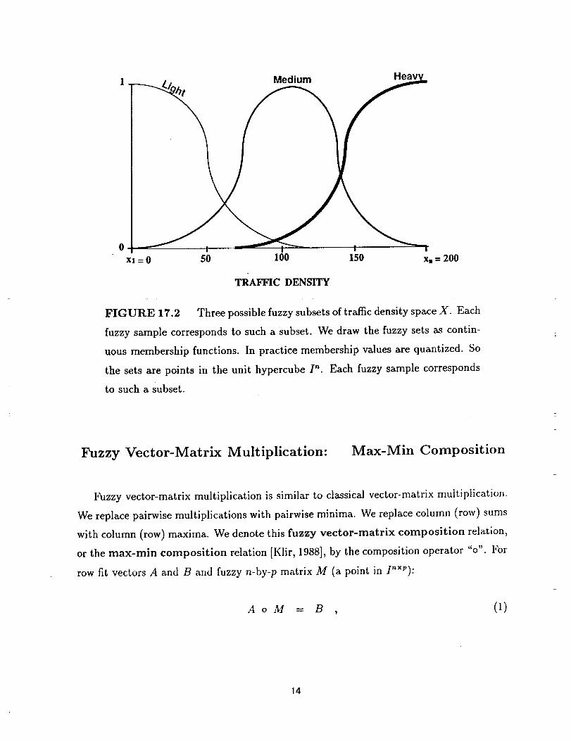
at hand. Intuitively the ai values should increase as the index i increases, perhaps ap-

proximating a sigmoid membership function. Figure 17.2 illustrates three possible fuzzy

subsets of the universe of discourse X.

13

1

0

xi=0

..__..._ /. Medium Heavy_

I -- I ' i

50 100 150 x. = 200

TRAFFIC DENSITY

FIGURE 17.2 Three possible fuzzy subsets of traffic density space X. Each

fuzzy sample corresponds to such a Subset. We draw the fuzzy sets as contin-

uous membership functions. In practice membership values are quantized. So

the sets are points in the unit hypercube I". Each fuzzy sample corresponds

to such a subset.

Fuzzy Vector-Matrix Multiplication: Max-Min Composition

Fuzzy vector-matrix multiplication is similar to classical vector-matrix multiplication.

We replace pairwise multiplications with pairwise minima. We replace column (row) sums

with column (row) maxima. We denote this fuzzy vector-matrix composition relation,

or the max-rain composition relation [Klir, 1988], by the composition operator "o'. For

row fit vectors A and B and fuzzy n-by-p matrix M (a point in I"×P):

AoM --- B , (1)

14

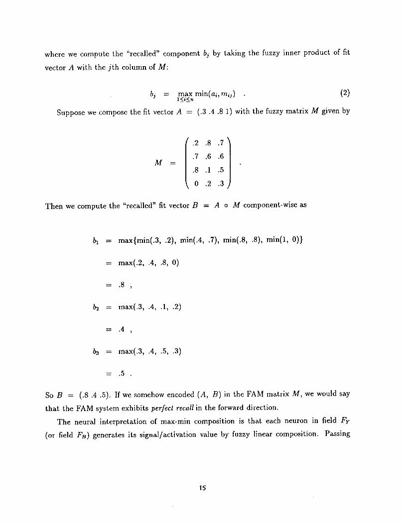
where we compute the "recalled" component bj by taking the fuzzy inner product of fit

vector A with the jth column of M:

b./ = max min(ai, mij) (2)l<i<n

Suppose we compose the fit vector A = (.3.4.8 1) with the fuzzy matrix M given by

m

.2 .8 .7

.7 ,6 .6

.8 .1 .5

0 .2 .3

Then we compute the "recalled" fit vector B = A o M component-wise as

b_ = max{min(.3, .2), min(.4, .7), min(.8, .8), min(1, 0)}

= max(.2, .4, .8, O)

_-- .8 ,

b2 = max(.3, .4, .1, .2)

= .4 ,

b3 = max(.3, .4, .5, .3)

= .5

So B = (.8.4 .5). If we somehow encoded (A, B) in the FAM matrix M, we would say

that the FAM system exhibits perfect recall in the forward direction.

The neural interpretation of max-min composition is that each neuron in field Fy

(or field FB) generates its signal]activation value by fuzzy linear composition. Passing

15

information back through M T allows us to interpret the fuzzy system as a bidirectional as-

sociative memory (BAM). The Bidirectional FAM Theorems below characterize successful

BAM recall for fuzzy correlation or Hebbian learning.

For completeness we also mention the max-product composition operator, which

replaces minimum with product in (2):

bj = max ai rnijI_<i_<,_

In the fuzzy literature this composition operator is often confused with the fuzzy correlation

encoding scheme discussed below. Max-product composition is a method for "multiply-

ing" fuzzy matrices or vectors. Fuzzy correlation, which also uses pairwise products of

fit values, is a method for constructing fuzzy matrices. In practice, and in the following

discussion, we use only max-min composition.

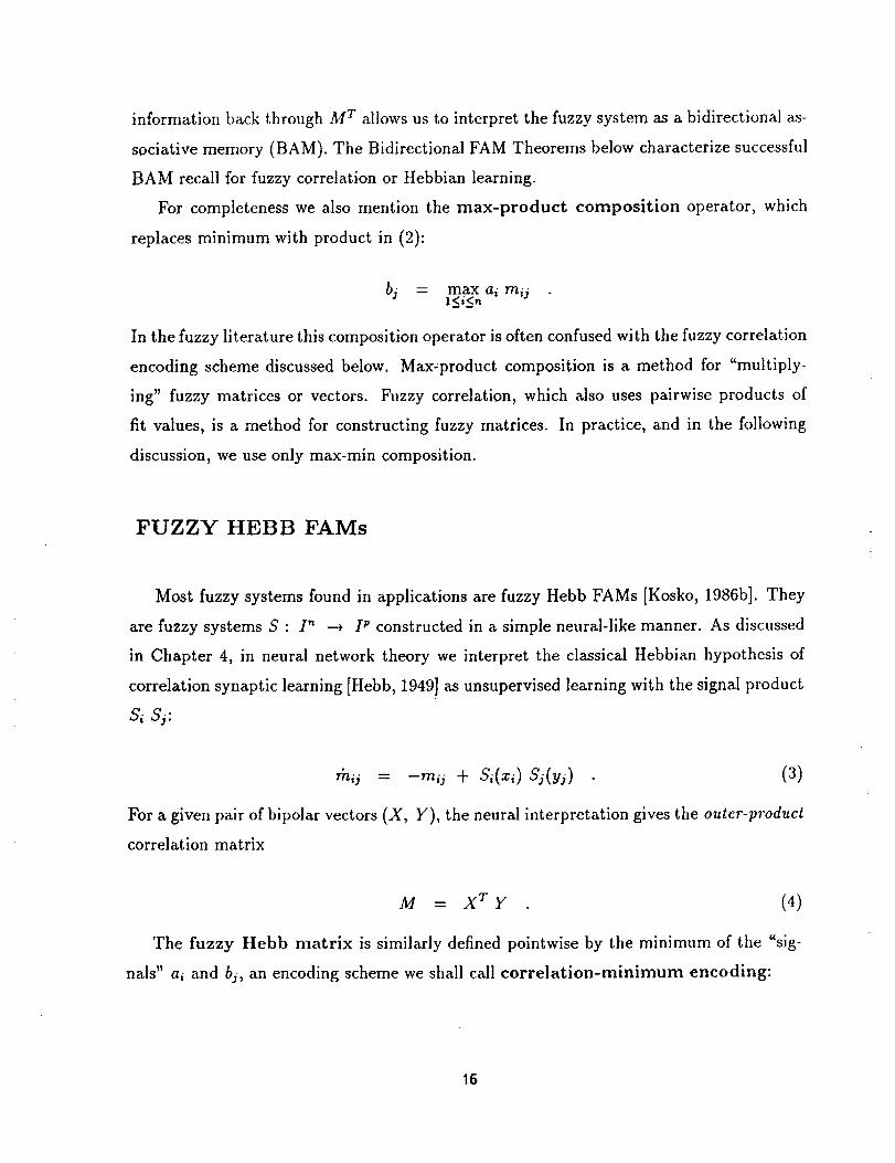
FUZZY HEBB FAMs

Most fuzzy systems found in applications are fuzzy Hebb FAMs [Kosko, 1986b]. They

are fuzzy systems S : I n _ I p constructed in a simple neural-like manner. As discussed

in Chapter 4, in neural network theory we interpret the classical Hebbian hypothesis of

correlation synaptic learning [Hebb, 1949] as unsupervised learning with the signal product

s, ss:

'% = -=,s + ss(ys) (3)

For a given pair of bipolar vectors (X, Y), the neural interpretation gives the outer-product

correlation matrix

M = X T Y (4)

The fuzzy Hebb matrix is similarly defined pointwise by the minimum of the "sig-

nals" ai and bj, an encoding scheme we shall call correlation-minimum encoding:

16

mij = min(ai, bj)

given in matrix notation as the fuzzy outer-product

(5)

M = A T o B (6)

Mamdani [1977] and Togai [1986] independently arrived at the fuzzy Hebbian prescrip-

tion (5) as a muXti-valued logical-implication operator: truth(a/ --* hi) = min(a_,bj).

The rain operator, though, is a symmetric truth operator. So it does not properly gen-

eralize the classical implication P --* Q, which is false if and only if the antecedent P

is true and the consequent Q is false, t(P) = 1 and t(Q) = 0. In contrast, a like desire

to define a "conditional possibility" matrix pointwise with continuous implication values

led Zadeh [1983] to choose the Lukasiewicz implication operator: mq = truth(ai --+

b_) = rain(l, 1 - a_ + bj). The problem with the Lukasiewicz operator is that it usually

unity. For rain(l, 1 - a_ + bj) < 1 iff a_ > bj. Most entries of the resulting matrix M

are unity or near unity. This ignores the information in the association (A, B). So A' o M

tends to equal the largest fit value a_, for any system input A'.

We construct an autoassociative fuzzy Hebb FAM matrix by encoding the redundant

pair (A, A) in (6), as the fuzzy auto-correlation matrix:

M = A T o A (7)

In the previous example the matrix M was such that the input A = (.3 .4 .8 1)

recalled fit vector B = (.8 .4 .5) upon max-min composition: A o M = B. Will

B still be recalled if we replace the original matrix M with the fuzzy Hebb matrix found

with (6)? Substituting A and B in (6) gives

M=AToB=

.3

.4

.8

1

o (.8 .4 .5) =

.3 .3 .3

.4 .4 .4

.8 .4 .5

.8 .4 .5

17

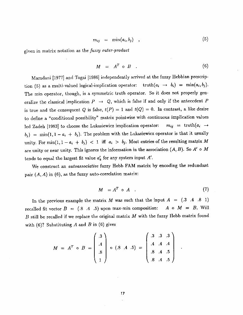
This fuzzy Hebb matrix M illustrates two key properties. First, the ith row of M is

the p_/irwise minimum of ai and the output associant B. Symmetrically, the jth column

of M is the pairwise minimum of bj and the input associant A:

aaAB

M =

a,_ A B

= [bx^ ATI ... Ibm^ AT] ,

where the cap operator denotes pairwise minimum: ai A bj

ai A B indicates component-wise minimum:

(8)

(9)

min(a_,bj). The term

ai ^ B = (a, A bl,...,ai ^ b,,) , (10)

Hence if some ak = 1, then the kth row of M is B. If some bt = 1, the lth column of

M is A. More generally, if some ak is at least as large as every bj, then the kth row of the

fuzzy Hebb matrix M is B.

Second, the third and fourth columns of M are just the fit vector B. Yet no column

is A. This allows perfect recall in the forward direction, A o M = B, but no$ in the

backward direction, B o M T _ A:

A o M = (.8 .4 .5) = B ,

B o M T = (.3 .4 .8 .8) = A' C A

A' is a proper subset of A • A' -_ A and S(A', A) = 1, where S measures the degree of

subsethood of A' in A, as discussed in Chapter 16. In other words, a_ <_ ai for each i and

a_, < ak for at least one k. The Bidirectional FAM Theorems below show that this is a

general property: If B _ = A o M differs from B, then B' is a proper subset of B. Hence

fuzzy subsets truly map to fuzzy subsets.

18

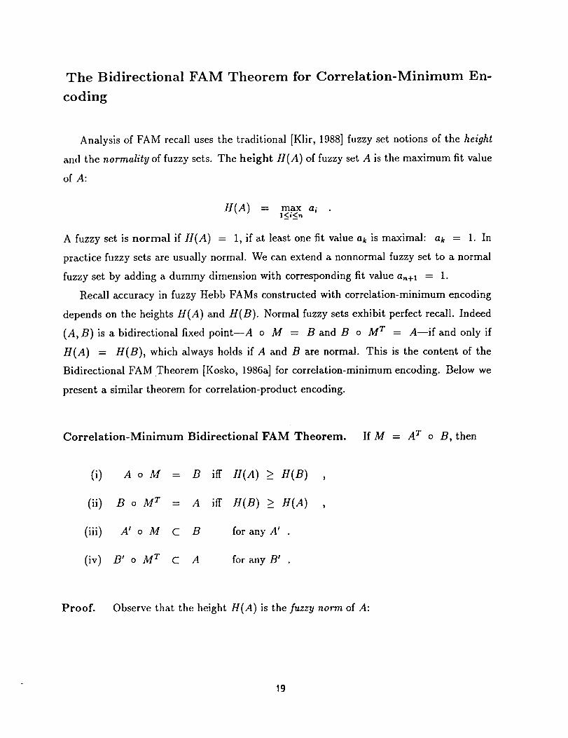
The Bidirectional FAM Theorem for Correlation-Minimum En-

coding

Analysis of FAM recall uses the traditional [Klir, 1988] fuzzy set notions of the height

and the normality of fuzzy sets. The height H(A) of fuzzy set A is the maximum fit value

of A:

H(A) = max ail_i<n

A fuzzy set is normal if H(A) = 1, if at least one fit value ak is maximal: ak = 1. In

practice fuzzy sets are usually normal. We can extend a nonnormal fuzzy set to a normal

fuzzy set by adding a dummy dimension with corresponding fit value a,,+l = 1.

Recall accuracy in fuzzy Hebb FAMs constructed with correlation-minimum encoding

depends on the heights H(A) and H(B). Normal fuzzy sets exhibit perfect recall. Indeed

(A,B) is a bidirectional fixed point--A o M = Band B o M r = A--if and only if

H(A) = H(B), which always holds if A and B are normal. This is the content of the

Bidirectional FAM Theorem [Kosko, 1986a] for correlation-minimum encoding. Below we

present a similar theorem for correlation-product encoding.

Correlation-Minimum Bidirectional FAM Theorem. If M = A T o B, then

(i) A o M = B iff H(A) > H(B)

(ii) B o M T = A iff H(B) > H(A)

(iii) A' o M C B for anyA'

(iv) B' o M T C A for any B'

Proof. Observe that the height H(A) is the fuzzy norm of A:

19

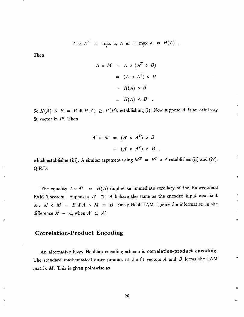
Then

A o A T = max al A ai = max ai = H(A)! I

A o M = A o (A T 0 B)

= (A o A T) o B

= H(A) o B

= H(A) A B

So H(A) A B = B iff H(A) > H(B), establishing (i). Now suppose A' is an arbitrary

fit vector in I n. Then

A' o M = (A' o A T ) o B

= (A' o A T ) A B ,

which establishes (iii). A similar argument using M T -- B r o A establishes (ii) and (iv).

Q.E.D.

The equality A o A T = H(A) implies an immediate corollary of the Bidirectional

FAM Theorem. Supersets A' D A behave the same as the encoded input associant

A" A _ o M = BifA o M = B. Fuzzy Hebb FAMs ignore the information in the

difference A' - A, when A' C A'.

Correlation-Product Encoding

An alternative fuzzy Hebbian encoding scheme is correlation-product encoding.

The standard mathematical outer product of the fit vectors A and B forms the FAM

matrix M. This is given pointwise as

2O

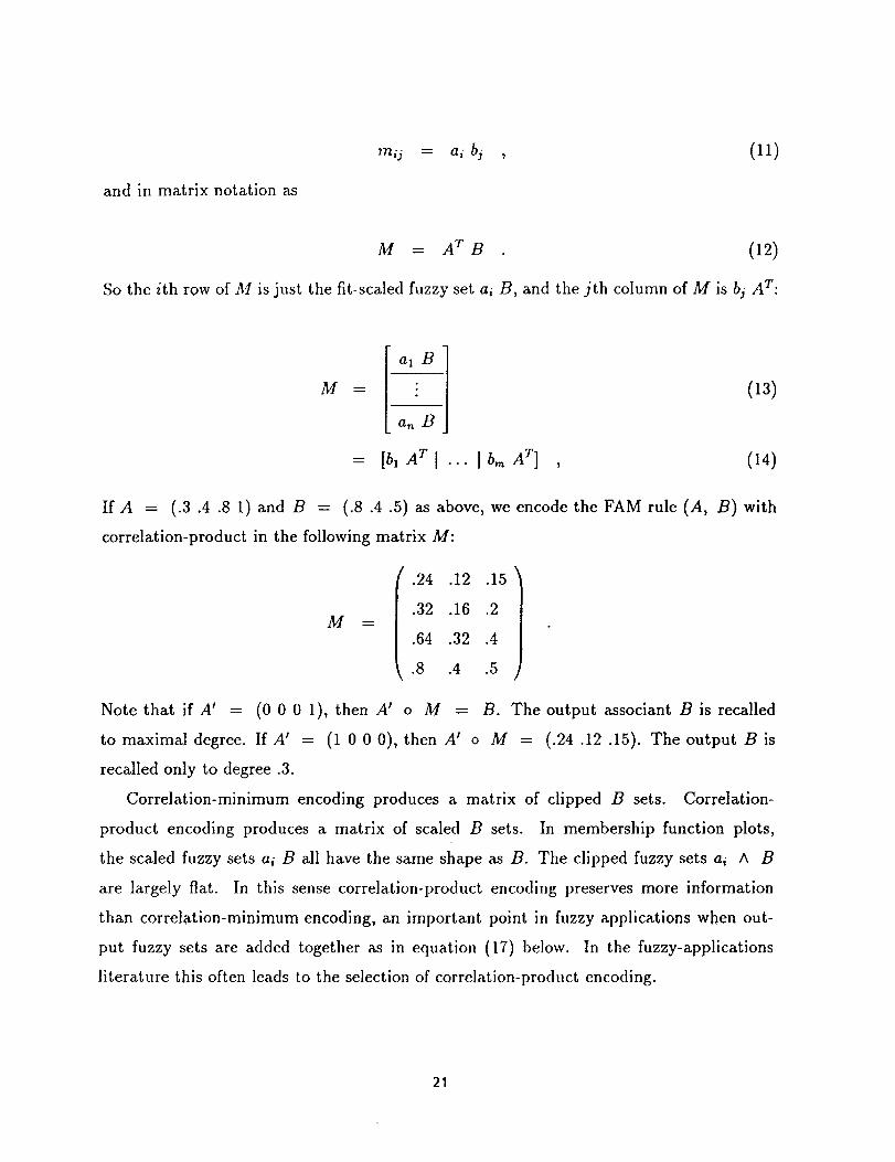
and in matrix notation as

mij = ai bs , (11)

M = A T B (12)

So the ith row of M is just the fit-scaled fuzzy set ai B, and the jth column of M is bs AT:

La- J= [b, A T] ... Ibm A T ] , (14)

IfA = (.3 .4.S 1) and B = (.8.4.5) as above, we encode the FAM rule (A, B) with

correlation-product in the following matrix M:

M __

.24 .12 .15

.32 .16 .2

.64 .32 .4

.8 .4 .5

Note that irA' = (0 0 0 1), then A' o M = B. The output associant Bis recalled

to maximal degree. IrA' = (1 000),then A' o M = (.24 .12.15). The output Bis

recalled only to degree .3.

Correlation-minimum encoding produces a matrix of clipped B sets. Correlation-

product encoding produces a matrix of scaled B sets. In membership function plots,

the scaled fuzzy sets ai B all have the same shape as B. The clipped fuzzy sets ai A B

are largely flat. In this sense correlation-product encoding preserves more information

than correlation-minimum encoding, an important point in filzzy applications when out-

put fuzzy sets are added together as in equation (17) below. In the fuzzy-applications

literature this often leads to the selection of correlation-product encoding.

21

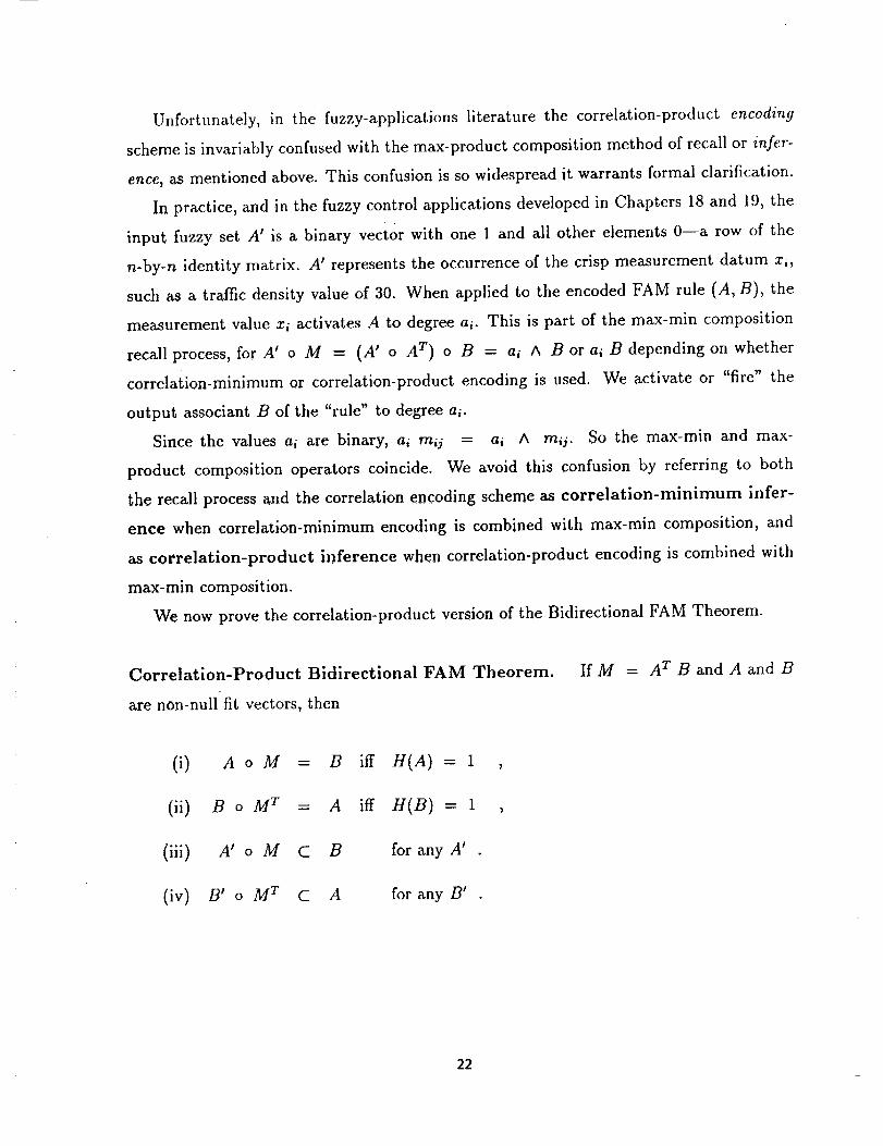
Unfortunately, in the fuzzy-applications literature the correlation-product encoding

scheme is invariably confilsed with the max-product composition method of recall or infer-

ence, as mentioned above. This confusion is so widespread it warrants formal clarification.

In practice, and in the fuzzy control applications developed in Chapters 18 and 19, the

input fuzzy set A' is a binary vector with one 1 and all other elements 0--a row of the

n-by-n identity matrix. A' represents the occurrence of the crisp measurement datum xi,

such as a traffic density value of 30. When applied to the encoded FAM rule (A, B), the

measurement value xi activates A to degree ai. This is part of the max-min composition

recall process, forA' o M = (A' o A T ) o B = ai A B or ai B depending on whether

correlation-minimum or correlation-product encoding is used. We activate or "fire" the

output associant B of the "rule" to degree ai.

Since the values ai are binary, ai rnij -= ai A mii. So the max-rain and max-

product composition operators coincide. We avoid this confusion by referring to both

the recall process and the correlation encoding scheme as correlation-minimum infer-

ence when correlation-minimum encoding is combined with max-rain composition, and

as correlation-product inference when correlation-product encoding is combined with

max-rain composition.

We now prove the correlation-product version of the Bidirectional FAM Theorem.

Correlation-Product Bidirectional FAM Theorem.

axe non-null fit vectors, then

If M = A T B and A and B

(i) A o M = B iff H(A) = 1 ,

(ii) B o M T = A iff H(B)= 1 ,

(iii) A' o M C B for anyA'

(iv) B' o M r C A for any B'

22

Proof.

AoM = A o (A T B)

= (A o A T) B

= H(A) B

Since B is not the empty set, H(A) B = B iff H(A) = 1, establishing (i). ( A o M = B

holds trivially if B is the empty set.) For an arbitrary fit vector A r in I_:

A'oM

since A' o A <_ H(A), establishing (iii).

i T = B T A. Q.E.D.

-_ (A' o A T) B

C H(A) B

C B ,

(ii) and (iv) are proved similarly using

Superimposing FAM Rules

Now suppose we have m FAM rules or associations (A1, B1),..., (A,,,, B,,). The fuzzy

Hebb encoding scheme (6) leads to rn FAM matrices M1,..., Mm to encode the associa-

tions. The natural neural-network temptation is to add, or in this case maximum, the m

matrices pointwise to distributively encode the associations in a single matrix M:

M = max Mk (15)l<k<m

This superimposition scheme fails for fuzzy Hebbian encoding. The superimposed result

tends to be the matrix ATo B, where A and B are the pointwise maximum of the respective

m fit vectors Ak and Bk. We can see this from the pointwise inequality

23

k (16)max min(ak, bk) < min( max ai, maxl<k<m -- l <k<iol 1 <_k<Ttl

Inequality (16) tends to hold with equality as m increases since all maximum terms ap-

proach unity. We lose the information in the m associations (Ak, Bk).

The fuzzy approach to the superimposition problem is to additively superimpose the m

recalled vectors B' k instead of the fuzzy Hebb matrices Mk. B'k and Mk are given by

A o Mk = A o (A T o Bk)

--

for any fit-vector input A applied in parallel to the bank of FAM rules (Ak, Bk). This

requires separately storing the m associations (Ak, Bk), as if each association in the FAM

bank were a separate feedforward neural network.

Separate storage of FAM associations is costly but provides an "audit trail" of the

FAM inference procedure. The user can directly determine which FAM rules contributed

how much membership activation to a "concluded" output. Separate storage also pro-

vides knowledge-base modularity. The user can add or delete FAM-structured knowledge

without disturbing stored knowledge. Both of these benefits are advantages over a pure

neural-network architecture for encoding the same associations (Ak, Bk). Of course we can

use neural networks exogenously to estimate, or even individually house, the associations

(Aj,,Bk).

Separate storage of FAM rules brings out another distinction between FAM systems

and neural networks. A fit-vector input A activates all the FAM rules (Ak, Bk) in parallel

but to different degrees. If A only partially "satisfies" the antecedent associant Ak, the

consequent associant Bk is only partially activated. If A does not satisfy Ak at all, Bk does

not activate at all. BS, is the null vector.

Neural networks behave differently. They try to reconstruct the entire association

(Ak, Bk) when stimulated with A. If A and Ak mismatch severely, a neural network will

24

tend to emit a non-null output B_, perhaps the result of the network dynamical system

falling into a "spurious" attractor in the state space. This may be desirable for metrical

classification problems. It is undesirable for inferential problems and, arguably, for associa-

tive memory problems. When we ask an expert a question outside his field of knowledge,

in many cases it is more prudent for him to give no response than to give an educated,

though wild, guess.

Recalled Outputs and "Defuzzification"

The recalled fit-vector output B is a weighted sum of the individual recalled vectors

BI,:

m

B = wkB; , (17)k=l

where the nonnegative weight wk summarizes the credibility or strength of the kth FAM

rule (Ak, Bk). The credibility weights wk are immediate candidates for adaptive modifica-

tion. In practice we choose wl .... =wm = 1 as a default.

In principle, though not in practice, the recalled fit-vector output is a normalized sum

of the B_ fit vectors. This keeps the components of B unit-interval valued. We do not

use normalization in practice because we invariably "defuzzify" the output distribution B

to produce a single numerical output, a single value in the output universe of discourse

Y = {Yl,...,Yp}. The information in the output waveform B resides largely in the

relative values of the membership degrees.

The simplest defuzzification scheme is to choose that element Ymax that has maximal

membership in the output fuzzy set B:

rnB(Ymax) = max mB(yj) (18)l_<j<k

The popular probabilistic methods of maximum-likelihood and maximum-a-posteriori pa-

rameter estimation motivate this maxinmm-membership defuzzification scheme. The

25

maximum-membershipscheme(18) is also computationally light.

There are two fundamental problemswith the maximum-membershipdefuzzification

scheme.First, the modeof the B distribution is not unique. This is especially troublesome

with correlation-minimum encoding, as the representation (8) shows, and somewhat less

troublesome with correlation-product encoding. Since the minimum operator clips off the

top of the Bk fit vectors, the additively combined output fit vector B tends to be flat over

many regions of universe of discourse Y. For continuous membership functions this leads

to infinitely many modes. Even for quantized fuzzy sets, there may be many modes.

In practice we can average multiple modes. For large FAM banks of "independent"

FAM rules, some form of the Central Limit Theorem (whose proof ultimately depends

on Fourier transformability not probability) tends to apply. The waveform B tends to

resemble a Gaussian membership function. So a unique mode tends to emerge. It tends

to emerge with fewer samples if we use c0rrelation-product encoding.

Second, the maximum-membership scheme ignores the information in much of the

waveform B. Again correlation-minimum encoding compounds the problem. In practice

B is often highly asymmetric, even if it is unimodal. Infinitely many output distributions

can share the same mode.

The natural alternative is the fuzzy centroid defuzzification scheme. We directly

compute the real-valued output as a normalized convex combination of fit values, the fuzzy

centroid [_ of fit-vector B with respect to output space Y:

P

Z: m (uj)/_ _ j=l- ), (19)

3=1

The fuzzy centroid is unique and uses all the information in the output distribution B. For

symmetric unimodal distributions the mode and fuzzy centroid coincide. In many cases

we must replace the discrete sums in (19) with integrals over continuously infinite spaces.

We show in Chapter 19, though, that for libraries of trapezoidal fuzzy sets we can replace

such a ratio of integrals with a ratio of simple discrete sums.

Note that computing the centroid (19) is the only step in the FAM inference procedure

26

that requiresdivision. All other operations are inner products, pairwise minima, and ad-

ditions. This promisesrealization in a fuzzy optical processor.Already someform of this

FAM-inference schemehas led to digital [Togai, 1986]and analog [Yamakawa,1987-88]

VLSI circuitry.

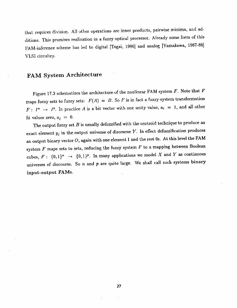
FAM System Architecture

Figure 17.3 schematizes the architecture of the nonlinear FAM system F. Note that F

maps fuzzy sets to fuzzy sets: F(A) = B. So F is in fact a fuzzy-system transformation

F : I n --_ IL In practice A is a bit vector with one unity value, ai = 1, and all other

fit values zero, aj = 0.

The output fuzzy set B is usually defuzzified with the centroid technique to produce an

exact element Y,i in the output universe of discourse Y. In effect defuzzification produces

an output binary vector O, again with one element 1 and the rest 0s. At this level the FAM

system F maps sets to sets, reducing the fuzzy system F to a mapping between Boolean

cubes, F : {0, 1} n --_ {0, 1} p. In many applications we model X and Y as continuous

universes of discourse. So n and p are quite large. We shall call such systems binary

input-output FAMs.

27

I- 1I I

I I

I I

I i

i I

A , ' = a-._ I ,_==,=_ i..._yj

i-

FAM Rule 1

FAM ule m

FAM SYSTEM

FIGURE 17.3 FAM system architecture. The FAM system F maps fuzzy

sets in the unit cube I" to fuzzy sets in the unit cube I p. Binary input fuzzy

sets are often used in practice to model exact input data. In general only an

uncertainty estimate of the system state is available. So A is a proper fuzzy set.

The user can defuzzify output fuzzy set B to yield exact output data, reducing

the FAM system to a mapping between Boolean cubes.

Binary Input-Output FAMs: Inverted Pendulum Example

Binary input-output FAMs (BIOFAMs) are the most popular fuzzy systems for appli-

cations. BIOFAMs map system state-variable data to control data. In the case of traffic

control, a BIOFAM maps traffic densities to green (and red) light durations.

BIOFAMs easily extend to multiple FAM rule antecedents, to mappings from product

cubes to product cubes. There has been little theoretical justification for this extension,

28

aside from Mamdani's [1977] original suggestion to multiply relational matrices. The ex-

tension to multi-antecedent FAM rules is easier applied than formally explained. In the

next section we present a general explanation for dealing with multi-antecedent FAM rules.

First, though, we present the BIOFAM algorithm by illustrating it, and the FAM construc-

tion procedure, on an archetypical control problem.

Consider an inverted pendulum. In particular, consider how to adjust a motor to bal-

ance an inverted pendulum in two dimensions. The inverted pendulum is a classical control

problem. It admits a math-model control solution. This provides a formal benchmark for

BIOFAM pendulum controllers.

There are two state variables and one control variable. The first state variable is the

angle 0 that the pendulum shaft makes with the vertical. Zero angle corresponds to the

vertical position. Positive angles are to the right of the vertical, negative angles to the left.

The second state variable is the angular velocity A0. In practice we approximate the

instantaneous angular velocity A0 as the difference between the present angle measurement

Ot and the previous angle measurement Or-l:

AOt = Ot -- Or-1

The control variable is the motor current or angular velocity vt. The velocity can also

be positive or negative. We expect that if the pendulum falls to the right, the motor

velocity should be negative to compensate. If the pendulum falls to the left, the motor

velocity should be positive. If the pendulum successfully balances at the vertical, the motor

velocity should be zero.

The real line R is the universe of discourse of the three variables. In practice we

restrict each universe of discourse to a comparatively small interval, such as [-90, 90] for

the pendulum angle, centered about zero.

We can quantize each universe of discourse into five overlapping fuzzy sets. We know

that the system variables can be positive, zero, or negative. We can quantize the magni-

tudes of the system variables finely or coarsely. Suppose we quantize.the magnitudes as

small, medium, and large. This leads to seven linguistic fuzzy set values:

29

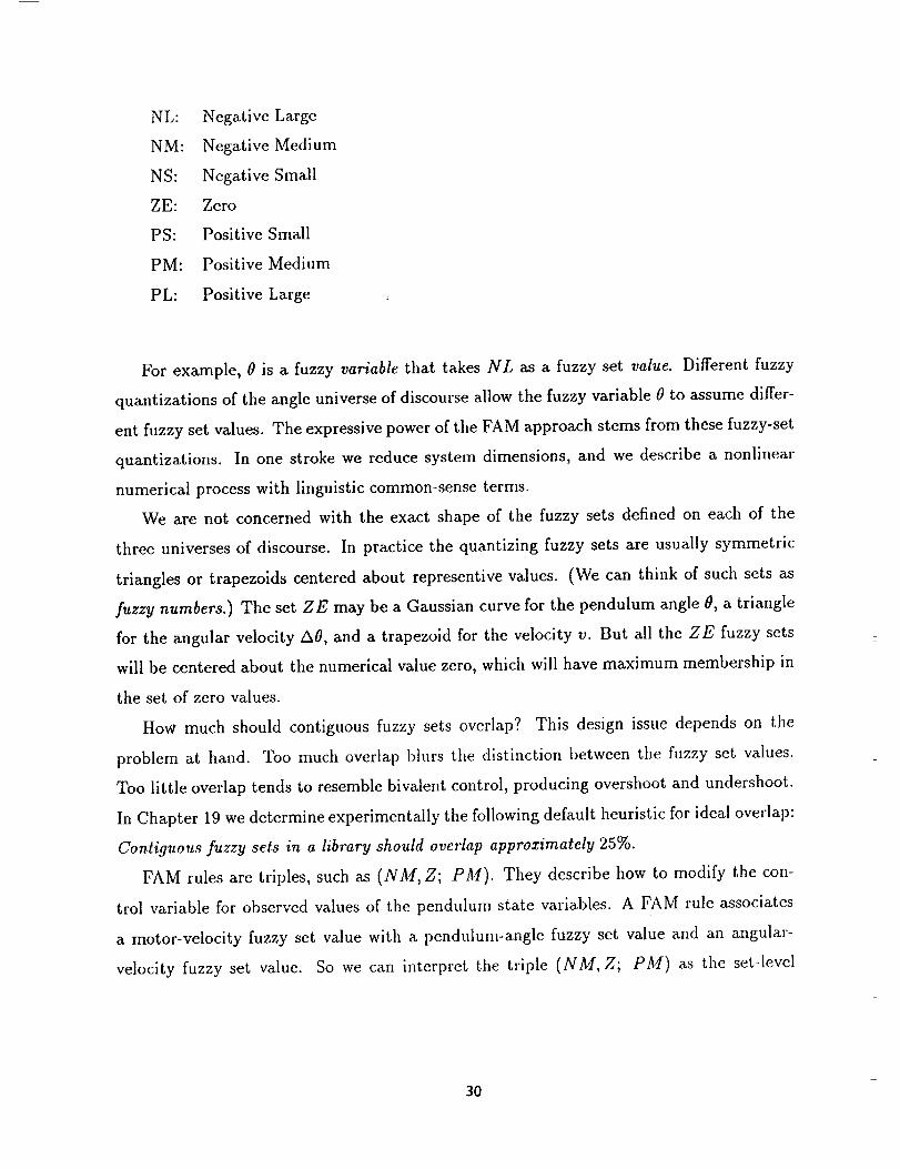
NL: Negative Large

NM: Negative Medium

NS: Negative Small

ZE: Zero

PS: Positive Small

PM: Positive Medium

PL: Positive Large

For example, 0 is a fuzzy variable that takes NL as a fuzzy set value. Different fuzzy

quantizations of the angle universe of discourse allow the fuzzy variable 0 to assume differ-

ent fuzzy set values. The expressive power of the FAM approach stems from these fuzzy-set

quantizations. In one stroke we reduce system dimensions, and we describe a nonlinear

numerical process with linguistic common-sense terms.

We are not concerned with the exact shape of the fuzzy sets defined on each of the

three universes of discourse. In practice the quantizing fuzzy sets are usually symmetric

triangles or trapezoids centered about representive values. (We can think of such sets as

fuzzy numbers.) The set ZE may be a Gaussian curve for the pendulum angle 0, a triangle

for the angular velocity A0, and a trapezoid for the velocity v. But all the ZE fuzzy sets

will be centered about the numerical value zero, which will have maximum membership in

the set of zero values.

How much should contiguous fuzzy sets overlap? This design issue depends on the

problem at hand. Too much overlap blurs the distinction between the fuzzy set values.

Too little overlap tends to resemble bivalent control, producing overshoot and undershoot.

In Chapter 19 we determine experimentally the following default heuristic for ideal overlap:

Contiguous fuzzy sets in a library should overlap approximately 25%.

FAM rules are triples, such as (NM, Z; PM). They describe how to modify the con-

trol variable for observed values of the pendulum state variables. A FAM rule associates

a motor-velocity fuzzy set value with a pendulum-angle fuzzy set value and an angular-

velocity fuzzy set value. So we can interpret the triple (NM, Z; PM) as the set-level

3O

implication

IF the pendulum angle0 is negative but medium

AND the angular velocity A0 is about zero,

THEN the motor velocity should be positive but medium.

These commonsensical FAM rules are comparatively easy to articulate in natural language.

Consider a terser linguistic version of the same three-antecedent FAM rule:

IF 0 = NM AND

THEN v = PM.

AO = ZE ,

Even this mild level of formalism may inhibit the knowledge acquisition process. On the

other hand, the still terser FAM triple (NM, ZE; PM) allows knowledge to be acquired

simply by filling in a few entries in a linguistic FAM-bank matrix. In practice this often

allows a working system to be developed in hours, if not minutes.

We specify the pendulum FAM system when we choose a FAM bank of two-antecedent

FAM rules. Perhaps the first FAM rule to choose is the steady-state FAM rule: (ZE, ZE; ZE).

The steady-state FAM rule describes what to do in equilibrium. For the inverted pendulum

we should do nothing.

This is typical of many control problems that require nulling a scalar error measure.

We can control multivariable problems by nulling the norms of the system error vector

and error-velocity vectors, or, better, by directly nulling the individual scalar variables.

(Chapter 19 shows how error nulling can control a realtime target tracking system.) Error

nulling tractably extends the FAM methodology to nonlinear estimation, control, and

decision problems of high dimension.

31

The pendulum FAM bank ",s a 7-by-7 matrix with linguistic fuzzy-set entries. We index

the columns by the seven fuzzy sets that quantize the angle 0 universe of discourse. We

index the rows by the seven fuzzy sets that quantize the angular velocity A0 universe of

discourse.

Each matrix entry is one of seven motor-velocity fuzzy-set values. Since a FAM rule is a

mapping or function, there is exactly one output velocity value for every pair of angle and

angular-velocity values. So the 49 entries in the FAM bank matrix represent the 49 possible

two-antecedent FAM rules. In practice most of the entries are blank. In the adaptive FAM

case discussed below, we adaptively generate the entries from process sample data.

Commonsense dictates the entries in the pendulum FAM bank matrix. Suppose the

pendulum is not changing. So A0 = ZE. If the pendulum is to the right of vertical,

the motor velocity should be negative to compensate. The farther the pendulum is to

the right, the larger the negative motor velocity should be. The motor velocity should

be positive if the pendulum is to the left. So the fourth row of the FAM bank matrix,

which corresponds to A0 = ZE, should be the ordinal inverse of the 0 row values. This

assignment includes the steady-state FAM rule (ZE, ZE; ZE).

Now suppose the angle 0 is zero but the pendulum is moving. If the angular velocity is

negative, the pendulum will overshoot to the left. So the motor velocity should be positive

to compensate. If the angular velocity is positive, the motor velocity should be negative.

The greater the angular velocity is in magnitude, the greater the motor velocity should

be in magnitude. So the fourth column of the FAM bank matrix, which corresponds to

0 = ZE, should be the ordinal inverse of the A0 column values. This assignment also

includes the steady-state FAM rule.

Positive 0 values with negative A0 values should produce negative motor velocity values,

since the pendulum is heading toward the vertical. So (PS, NS; NS) is a candidate FAM

rule. Symmetrically, negative 0 values with positive A0 values should produce positive

motor velocity values. So (NS, PS; PS) is another candidate FAM rule.

This gives 15 FAM rules altogether. In practice these rules are more than sufficient to

successfully balance an inverted pendulum. Different, and smaller, subsets of FAM rules

may also successfully balance the pendulum.

32

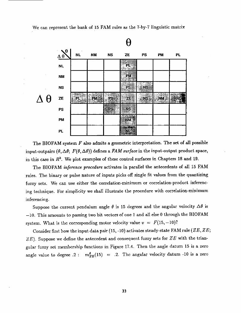
We can represent the bank of 15 FAM rules as the 7-by-7 linguistic matrix

0A, NS ZE PS

:_,:__¢::: :_: _ _::: ::::::::::::::::::::::::::::::::

..................... _:__'..._:_.._:_,:_;:_:_7_._:_::::::_:_:_:_:_ ....... _i_i_i:.ii_i_ ::_ :....._:_:;;:_::_>!i !!_.:-':_i_'_?'.,'i_:_i_._i_ ::::::::::::::::::::::::::::::::::: _" _'_'_"_ _'

.............NS....PS

PM _M22_

NL NM PM PL

The BIOFAM system F also admits a geometric interpretation. The set of all possible

input-outpalrs (_, A_; F(t_, AO)) defines a FAM surface in the input-output product space,

in this case in R 3. We plot examples of these control surfaces in Chapters 18 and 19.

The BIOFAM inference procedure activates in parallel the antecedents of all 15 FAM

rules. The binary or pulse nature of inputs picks off single fit values from the quantizing

fuzzy sets. We can use either the correlation-minimum or correlation-product inferenc-

ing technique. For simplicity we shall illustrate the procedure with correlation-minimum

inferencing.

Suppose the current pendulum angle _ is 15 degrees and the angular velocity AO is

-10. This amounts to passing two bit vectors of one 1 and all else 0 through the BIOFAM

system. What is the corresponding motor velocity value v = F(15,-10)?

Consider first how the input data pair (15, -10) activates steady-state FAM rule (ZE, ZE;

ZE). Suppose we define the antecedent and consequent fuzzy sets for ZE with the trian-

gular fuzzy set membership functions in Figure 17.4. Then the angle datum 15 is a zero

angle value to degree .2 : m_s(15) = .2. The angular velocity datum -10 is a zero

33

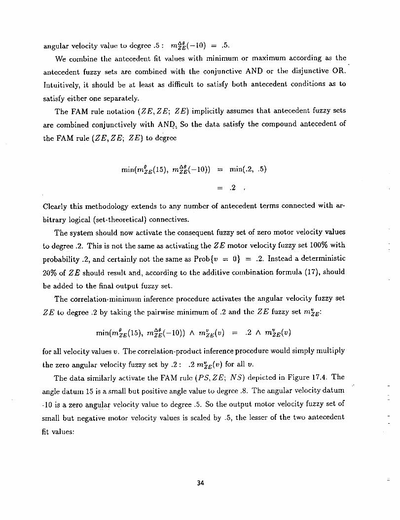
angular velocity value to degree .5: m_(-10) = .5.

We combine the antecedent fit values with minimum or maximum according as the

antecedent fuzzy sets are combined with the conjunctive AND or the disjunctive OR.

Intuitively, it should be at least as difficult to satisfy both antecedent conditions as to

satisfy either one separately.

The FAM rule notation (ZE, ZE; ZE) implicitly assumes that antecedent fuzzy sets

are combined conjunctively with AND. So the data satisfy the compound antecedent of

the FAM rule (ZE, ZE; ZE) to degree

min(mazE(15), A0rnzE(--lO)) = min(.2, .5)

= .2

Clearly this methodology extends to any number of antecedent terms connected with ar-

bitrary logical (set-theoretical) connectives.

The system should now activate the consequent fuzzy set of zero motor velocity values

to degree .2. This is not the same as activating the ZE motor velocity fuzzy set 100% with

probability .2, and certainly not the same as Prob{v = 0} = .2. Instead a deterministic

20% of ZE should result and, according to the additive combination formula (17), should

be added to the final output fuzzy set.

The correlation-minimum inference procedure activates the angular velocity fuzzy set

ZE to degree .2 by taking the pairwise minimum of .2 and the ZE fuzzy set m_E:

min(m_E(15), A0mz (-10)) ^ = .9 ^ m E(v)

for all velocity values v. The correlation-product inference procedure would simply multiply

the zero angular velocity fuzzy set by .2: .2 m_zE(V) for all v.

The data similarly activate the FAM rule (PS, ZE; NS) depicted in Figure 17.4. The

angle datum 15 is a small but positive angle value to degree .8. The angular velocity datum

-10 is a zero angular velocity value to degree .5. So the output motor velocity fuzzy set of

small but negative motor velocity values is scaled by .5, the lesser of the two antecedent

fit values:

34

min(mOs(15), mzE(_lO)),x0 A m_s(V ) = .5 A m°Ns(V)

for all velocity values v. So the data activate the FAM rule (PS, ZE; NS) to_reater degree

than the steady-state FAM rule (ZE, ZE; ZE) since in this example an angle value of 15

degrees is more a small but positive angle value than a zero angle value.

The data similarly activate the other 13 FAM rules. We combine the resulting minimum-

scaled consequent fuzzy sets according to (17) by summing pointwise. We can then com-

pute the fuzzy centroid with equation (19), with perhaps integrals replacing the discrete

sums, to determine the specific output motor velocity v. In Chapter 19 we show that, for

symmetric fuzzy sets of quantization, the centroid can always be computed exactly with

simple discrete sums even if the fuzzy sets are continuous. In many realtime applications

we must repeat this entire FAM inference procedure hundreds, perhaps thousands, of times

per second. This requires fuzzy VLSI or optical processors.

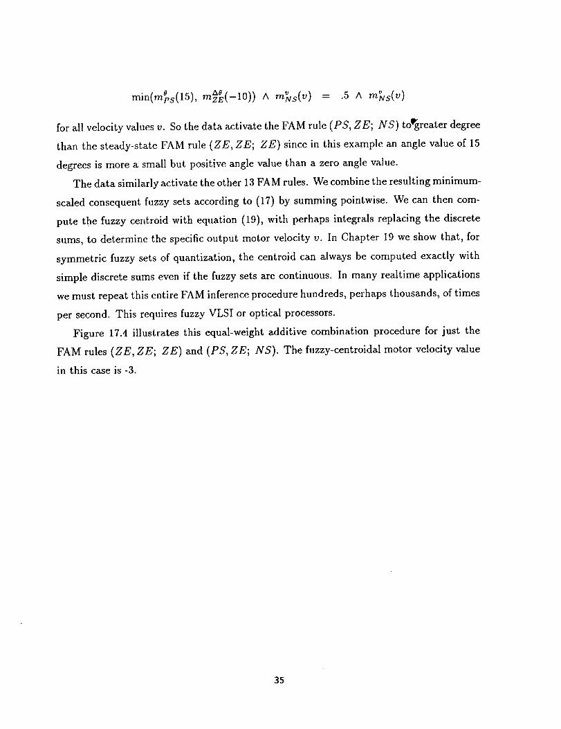
Figure 17.4 illustrates this equal-weight additive combination procedure for just the

FAM rules (ZE, ZE; ZE) and (PS, ZE; NS). The fuzzy-centroidal motor velocity value

in this case is -3.

35

PS

_ ÷r

0

ZE

e

FAM Rule ( PS, NS, NS )

[IF e- PsAND_. Ze.JzE 'IT"_v=NS I NS

...........I0 0 * 0

_0 V

m4-

FAM Rule ( ZE,, ZE ; ZE )

IF O=ZE AND _ =ZE,]THEN V=ZEZE ZE

i;-:--:-/- .........- -- _qo o - o

l &B V

. " 4-

i V!

_, c,_ [_

FIGURE 17.4 FAM correlation-minimum inference procedure. The FAM

system consists of the two two-antecedent FAM rules (PS, ZE; NS) and

(ZE, ZE; ZE). The input angle datum is 15, and is more a small but pos-

itive angle value than a zero angle value. The input angular velocity datum

is -10, and is only a zero angular velocity value to degree .5. Antecedent fit

values are combined with minimum since the antecedent terms are combined

conjunctively with AND. The combined fit value then scales the consequent

fuzzy set with pairwise minimum. The minimum-scaled output fuzzy sets are

added pointwise. The fuzzy centroid of this output waveform is computed and

yields the system output velocity value -3.

Multi-Antecedent FAM Rules: Decompositional Inference

The BIOFAM inference procedure treats antecedent fuzzy sets as if they were propo-

sitions with fuzzy truth values. This is because fuzzy logic corresponds to 1-dimensional

36

fuzzy set theory and because we use binary or exact inputs. We now formally develop the

connection between BIOFAMs and the FAM theory presented earlier.

Consider the compound FAM rule "IF X is A AND Y is B , THEN 6' is Z,"

or (A, B; C) for short. Let the universes of discourse X, Y, and Z have dimensions n, p,

andq: X = {zl,...,z,},Y = {y,,...,yp},andZ = {zl,...,zq}. We can directly

extend this framework to multiple antecedent and consequent terms.

In our notation X, Y, and Z are both universes of discourse and fuzzy variables. The

fuzzy variable X can assume the fuzzy set values A1,A2,..., and similarly for the fuzzy

variables Y and Z. When controlling an inverted pendulum, the identification "X is A"

might represent the natural-language description "The pendulum angle is positive but

small."

What is the matrix representation of the FAM rule (A, B; (7)? The question is nontriv-

ial since A, B, and 6' are fuzzy subsets of different universes of discourse, points in different

unit cubes. Their dimensions and interpretations differ. Mamdani [1977] and others have

suggested representing such rules as fuzzy multidimensional relations or arrays. Then the

FAM rule (A, B; C) would be a fuzzy subset of the product space X x Y x Z. This rep-

resentation is not used in practice since only eXaCt inputs are presented to FAM systems

and the BIOFAM procedure applies. If we presented the system with a genuine fuzzy set

input, we would no doubt preprocess the fuzzy set with a centroidal or maximum-fit-value

technique so we could still apply the BIOFAM inference procedure.

We present an alternative representation that decomposes, then recomposes, the FAM

rule (A, B; C) in accord with the FAM inference procedure. This representation allows

neural networks to adaptively estimate, store, and modify the decomposed FAM rules. The

representation requires far less storage than the multidimensional-array representation.

Let the fuzzy Hebb matrices MAc and Msc store the simple FAM associations (A, 6')

and (B, C):

MAc = A T o C , (20)

Mso = B T o C (21)

37

The fuzzy Hebb matrices Mac and MBc split the compound FAM rule (A, B; C). We can

construct the splitting matrices with correlation-product encoding.

Let Ij¢ -- (0... 0 1 0... 0) be an n-dimensional bit vector with ith element 1 and all

other elements 0. I,_. is the ith row of the n-by-n identity matrix. Similarly, I_, and I_ are

the respective jth and kth rows of the p-by-p and q-by-q identity matrices. The bit vector

I_ represents the occurrence of the exact input xi.

We will call the proposed FAM representation scheme FAM deeornpositional infer-

ence, in the spirit of the max-min compositional inference scheme discussed above. FAM

decompositional inference decomposes the compound FAM rule (A, B; C) into the com-

ponent rules (A, C) and (B, C). The simpler component rules are processed in parallel.

New fuzzy set inputs A' and B' pass through the FAM matrices Mac and MBc. Max-min

composition then gives the recalled fuzzy sets Ca, and CB,:

Ca, = A' o MAC , (22)

C6, = B' o MBc (23)

The trick is to recompose the fuzzy sets CA, and CB, with intersection or union according

as the antecedent terms "X is A" and "Y is B" are combined with AND or OR. The negated

antecedent term "X is NOT A" requires forming the set complement C_, for input fuzzy

set A'.

Suppose we present the new inputs A' and B' to the single-FAM-rule system F that

stores the FAM rule (A, B; C). Then the recalled output fuzzy set C' equals the intersec-

tion of CA, and CB,:

F(A', B') = [A' o MAC] N [B' o MBc]

= CA, N CB,

We can then defuzzify C', if we wish, to yield the exact output I k.

(24)

38

The logical connectivesapply to the antecedentterms of different dimensionand mean-

ing. Decompositionalinferenceappliesthe set-theoreticanaloguesof the logical connectives

to subsetsof Z. Of course all subsets G' of Z have the same dimension and meaning.

We now prove that decompositional inference generalizes BIOFAM inference. This gen-

eralization is not simply formal. It opens an immediate path to adaptation with arbitrary

neural network techniques.

Suppose we present the exact inputs xi and yj to the single-FAM-rule system F that

stores (A, B; C). So we present the unit bit vectors I_ and I_ to F as nonfuzzy set inputs.

Then

F(x,,uj) = F(5,, /¢) = [I_ o MAcl n [I_ o MBc]

= a_^C n bj ^C

= min(ai, b./) A C

(25)

(26)

(25) follows from (8). Representing G with its membership function me, (26) is equivalent

to the BIOFAM prescription

min(a,, bj) ^ me(z) (27)

for all z in Z.

If we encode the simple FAM rules (A, C) and (B, C) with correlation-product encoding,

decompositional inference gives the BIOFAM version of correlation-product inference:

F(Px, I_) = [I_x o ATcI n [I_ o BTcI

= aiC Cl biC (28)

= min(ai, bi) C (29)

= min(ai, bj) me(z) (30)

for all z in Z. (13) implies (28). man(a/ck, bj ck) = min(ai, bj) ck implies (29).

39

Decompositional inferenceallows arbitrary fuzzy sets, waveforms,or distributions A'

and B' to be applied to a FAM system. The FAM systemcan housean arbitrary FAM

bank of compound FAM rules. If weuse the FAM systemto control a process,the input

fuzzy sets A t and B' can be the output of an independent state-estimation system, such

as a Kalman filter. A' and B' might then represent probability distributions on the exact

input spaces X and Y. The filter-controller cascade is a common engineering architecture.

We can split compound consequents as desired. We can split the compound FAM rule

"IF X is A AND Y is B,THEN Z is C OR W is D,"or(A,B; C,D),

into the FAM rules (A, B; C) and (A, B; D). We can use the same split if the consequent

logical connective is AND.

We can give a propositional-calculus justification for the decompositional inference

technique. Let A, B, and C be bivalent propositions with truth values t(A), t(B), and

t(C) in {0, 1}. Then we can construct truth tables to prove the two consequent-splitting

tautologies that we use in decompositional inference:

[A (B OR C)] ---, [(A B) Oa (A ---* C)]

[a _ (BANDC)] ----* [(A _ B) AND (A ----* C)]

where the arrow represents logical implication.

, (31)

, (32)

In bivalent logic, the implication A ---* B is false iff the antecedent A is true and the

consequent B is false. Equivalently, t(A --* B) = 1 iff t(A) = 1 and t(B) = O.

This allows a "brief" truth table to be constructed to check for validity. We chose truth

values for the terms in the consequent of the overall implication (31) or (32) to make

the consequent false. Given those restrictions, if we cannot find truth values to make the

antecedent true, the statement is a tautology. In (31), if t((A _ B) OR (A ---* C)) = 0,

then t(A) = 1 and t(B) = t(C) = 0, since a disjunction is false iff both disjuncts are

false. This forces the antecedent A --* (B OR C) to be false. So (31) is a tautology: It

is true in all cases.

We can also justify splitting the compound FAM rule "IF X is A OR Y is B ,

THEN Z is C " into the disjunction (union) of the two simple FAM rules "IF X is A,

40

THEN Z is C " and "IF Y is B, THEN Z is C" with a propositional tautology:

[(A OR B) _ C] _ [(A _ C) OR (B_ C)] (33)

Now consider splitting the original compound FAM rule "IF X is A AND Y is B,

THEN Z is C " into the conjunction (intersection) of the two simple FAM rules "IF X

is A,THEN Z is C" and "IF Y is B,THEN Z is C." A problem arises when

we examine the truth table of the corresponding proposition

[(A AND B) ----* C] _ [(A _ C) AND (B _ C)] (34)

The problem is that (34) is not always true, and hence not a tautology. The implication

is false if A is true and B and C are false, or if A and C are false and B is true. But the

implication (34) is valid if both antecedent terms A and B are true. So if t(A) = t(B) = 1,

the compound conditional (A AND B)_ C implies both A ---* C and B ---* C.

The simultaneous occurrence of the data values xi and yj satisfies this condition. Recall

that logic is 1-dimensional set theory. The condition t(A) = t(B) = 1 is given by the 1 in

I_¢ and the 1 in I_.. We can interpret the unit bit vectors Ij¢ and I_, as the (true) bivalent

propositions "X is xi" and "Y is Yi." Propositional logic applies coordinate-wise. A

similar argument holds for the converse of (33).

For general fuzzy set inputs A' and B' the argument still holds in the sense of continuous-

valued logic. But the truth values of the logical implications may be less than unity while

greater than zero. If A' is a null vector and B' is not, or vice versa, the implication (34)

is false coordinate-wise, at least if one coordinate of the non-null vector is unity. But in

this case the decompositional inference scheme yields an output null vector C'. In effect

the FAM system indicates the propositional falsehood.

Adaptive Decompositional Inference

The decompositional inference scheme allows the splitting matrices MAC and MBc to

41

be arbitrary. Indeedit allows them to be eliminated altogether.

Let Nx : I" _ I q be an arbitrary neural network system that maps fuzzy subsets A'

of X to fuzzy subsets C' of Z. Nv : I p _ I q can be a different neural network. In general

Nx and Nr" are time-varying.

The adaptive decompositional inference (ADI) scheme allows compound FAM rules to

be adaptively split, stored, and modified by arbitrary neural networks. The compound

FAMrule U!F X is A AND Y is B, THEN Z is C," or (A,B; C),can be split

by Nx and Nv. Nx can house the simple FAM association (A, C). Nr" can house (B, C).

Then for arbitrary fuzzy set inputs A' and B', ADI proceeds as before for an adaptive

FAMsystemF: I"xI p _ I q that houses theFAM rule(A,B; C) orabank of such

FAM rules:

F(A',B') = Nx(A') n Ny(B') (35)

= CA, nCs,

= C'

Any neural network technique can be used. A reasonable candidate for many un-

structured problems is the backpropagation algorithm applied to several small feedforward

multilayer networks. The primary concerns are space and training time. Several small

neural networks can often be trained in parallel faster, and more accurately, than a single

large neural network.

The ADI approach illustrates one way neural algorithms can be embedded in a FAM

architecture. Below we discuss another way that uses unsupervised clustering algorithms.

ADAPTIVE FAMs:

IN FAM CELLS

PRODUCT-SPACE CLUSTERING

An adaptive FAM (AFAM) is a time-varying mapping between fuzzy cubes. In

principle the adaptive decompositional inference technique generates AFAMs. But we

42

shall reservethe label AFAM for systemsthat generateFAM rules from training data but

that do not requiresplitting and recombiningFAM data.

We proposea geometricAFAM procedure.The procedureadaptively clusters training

samplesin the FAM systeminput-output product space. FAM mappings are balls or clusters

in the input-output product space. These clusters are simply the fuzzy Hebb matrices

discussed above. The procedure "blindly" generates weighted FAM rules from training

data. Further training modifies the weighted set of FAM rules. We call this unsupervised

procedure product-space clustering.

Consider first a discrete 1-dimensional FAM system S : I n ---, I p. Then a FAM rule

has the form "IF X is Ai , THEN Y is Bi " or (Ai, Bi). The input-output product

space is I" x I v.

What does the FAM rule (Ai, Bi) look like in the product space I n × Iv? It'looks like a

cluster of points centered at the numerical point (Ai, Bi). The FAM system maps points

A near Ai to points B near Bi. The closer A is to Ai, the closer the point (A, B) is to the

point (Ai, Bi) in the product space I" × I v. In this sense FAMs map balls in I n to balls

in I v. The notation is ambiguous since (Ai, Bi) stands for both the FAM rule mapping,

or fuzzy subset of I n x IP, and the numerical fit-vector point in I n x I v.

Adaptive clustering algorithms can estimate the unknown FAM rule (Ai, Bi) from train-

ing samples of the form (A, B). In general there are m unknown FAM rules (Aa, B1), ...,

(An, Bin). The number m of FAM rules is also unknown. The user may select m arbitrarily

in many applications.

Competitive adaptive vector quantization (AVQ) algorithms can adaptively estimate

both the unknown FAM rules (Ai, Bi) and the unknown number m of FAM rules from

FAM system input-output data. The AVQ algorithms do not require fuzzy-set data. Scalar

BIOFAM data suffices, as we illustrate below for adaptive estimation of inverted-pendulum

control FAM rules.

Suppose the r fuzzy sets A1, ..., Ar quantize the input universe of discourse X. The

s fuzzy sets B1, ..., B, quantize the output universe of discourse Y. In general r and s

are unrelated to each other and to the number m of FAM rules (Ai, Bi). The user must

specify r and s and the shape of the fuzzy sets Ai and Bi. In practice this is not difficult.

43

Quantizing fuzzy sets are usually trapezoidal, and r and s are less than 10.

The quantizing collections {Ai} and {Bj} define rs FAM cells F_j in the input-output

product space I" × I p. The FAM cells Fij overlap since contiguous quantizing fuzzy sets Ai

and A_+x, and Bj and Bj+1, overlap. So the FAM cell collection {Fq} does not partition

the product space I" × I p. The union of all FAM cells also does not equal I" × I p since

the patches Fij are fuzzy subsets of I n × I p. The union provides only a fuzzy "cover" for

I s × I p.

The fuzzy Cartesian product A_ × B_ defines the FAM cell F#. A_ x B_ is just the

fuzzy outer product A T o B_ in (6) or the correlation product A T B, in (12). So a FAM cell

F_j is simply the fuzzy correlation-minimum or correlation-product matrix M_j : Fij = Mii.

Adaptive FAM Rule Generation

Let lnl,...,rnk be k quantization vectors in the input-output product space I" × I p

or, equivalently, in I n+p. mj is the jth column of the synaptic connection matrix M. M

has n + p rows and k columns.

Suppose, for instance, mj changes in time according to the differential competitive

learning (DCL) AVQ algorithm discussed in Chapters 6 and 9. The competitive system

samples concatenated fuzzy set samples of the form [AIB ]. The augmented fuzzy set IAIB]

is a point in the unit hypercube I '*+p.

The synaptic vectors rnj converge to FAM matrix centroids in I" x IP. More generally

they estimate the density or distribution of the FAM rules in I '_ x I p. The quantizing

synaptic vectors naturally weight the estimated FAM rule. The more synaptic vectors

clustered about a centroidal FAM rule, the greater its weight wi in (17).

Suppose there are 15 FAM-rule centroids in I" x I p and k > 15. Suppose k, synaptic

vectors rnj cluster around the ith centroid. So kx + ... + kls = k. Suppose the cluster

counts kl are ordered as

44

The first centroidal FAM rule is as at least as frequent as the second centroidal FAM

rule, and so on. This gives the adaptive FAM-rule weighting scheme

]_i

w, = _ (37)

The FAM rule weights wi evolve in time as new augmented fuzzy sets [AJB] are sampled.

In practice we may want only the 15 most-frequent FAM rules or only the FAM rules with

at least some minimum frequency Wmln. Then (37) provides a quantitative solution.

Geometrically we count the number k O of quantizing vectors in each FAM cell F O. We

can define FAM-cell boundaries in advance. High-count FAM cells outrank low-count FAM

ceils. Most FAM cells contain zero or few synaptic vectors.

Product-space clustering extends to compound FAM rules and product spaces. The

FAM rule "IF X is A AND Y is B, THEN Z is C", or (A, B; C), is a point in

I '_ × I p x I q. The t fuzzy sets C1,...,Ct quantize the new output space Z. There are

rst FAM cells F_jk. (36) and (37) extend similarly. X, Y, and Z can be continuous, The

adaptive clustering procedure extends to any number of FAM-rule antecedent terms.

Adaptive BIOFAM Clustering

BIOFAM data clusters more efficiently than fuzzy-set FAM data. Paired numbers are

easier to process and obtain than paired fit vectors. This allows system input-output data

to directly generate FAM systems.

In control applications, human or automatic controllers generate streams of "well-

controlled" system input-output data. Adaptive BIOFAM clustering converts this data

to weighted FAM rules. The adaptive system transduces behavioral data to behavioral

rules. The fuzzy system learns causal patterns. It learns which control inputs cause which

control outputs. The system approximates these causal patterns when it acts as the con-

troller.

Adaptive BIOFAMs cluster in the input-output product space X × Y . The product

space X x Y is vastly smaller than the power-set product space I _ x I p used above. The

45

adaptive synaptic vectors mj are now 2-dimensionalinstead of n + p-dimensional. On

the other hand, competitive BIOFAM clustering requires many more input-output data

pairs (xi, yi) _ R 2 than augmented fuzzy-set samples [A]B] _ I =+p.

Again our notation is ambiguous. We now use x/ as the numerical sample from X

at sample time i. Earlier xi denoted the ith ordered element in the finite nonfuzzy set

X = {xl,...,x,,}. One advantage is X can be continuous, say R".

BIOFAM clustering counts synaptic quantization vectors in FAM cells. The system

samples the nonfuzzy input-output stream (z_, y_), (z2, y2),... Unsupervised competitive

learning distributes the k synaptic quantization vectors ml,..., mk in X × Y. Learning

distributes them to different FAM cells Fij. The FAM cells Fij overlap but are nonfuzzy

subcubes of X × Y. The BIOFAM FAM cells Fij cover X × Y.

Fij contains kij quantization vectors at each sample time. The cell counts k_j define a

frequency histogram since all kij sum to k. So wij _ weights the FAM rule "IF X is= k

Ai, THEN Y is Bj."

Suppose the pairwise-overlapping fuzzy sets N L, N M, N S, Z E, P S, P M, P L quan-

tize the input space X. Suppose seven similar fuzzy sets quantize the output space Y. We

can define the fuzzy sets arbitrarily. In practice they are normal and trapezoidal. (The

boundary fuzzy sets NL and PL are ramp functions.) X and Y may each be the real line.

A typical FAM rule is "IF X is NL, THEN Y is PS."

Input datum zi is nonfuzzy. When X = xl holds, the relations X = NL,..., X = PL

hold to different degrees. Most hold to degree zero. X = NM holds to degree mlVM(Zi).

Input datum xi partially activates the FAM rule "IF X is NM, THEN Y is ZE" or,

equivalently, (NM; ZE). Since the FAM rules have single antecedents, xi activates the

consequent fuzzy set ZE to degree mNM(zi) as weIl. Multi-antecedent FAM rules activate

output consequent sets according to a logic-based function of antecedent term membership

values, as discussed above on BIOFAM inference.

Suppose Figure 17.5 represents the input-output data stream (x_, yl), (x2, y2),.., in the

planar product space X × Y:

46

×

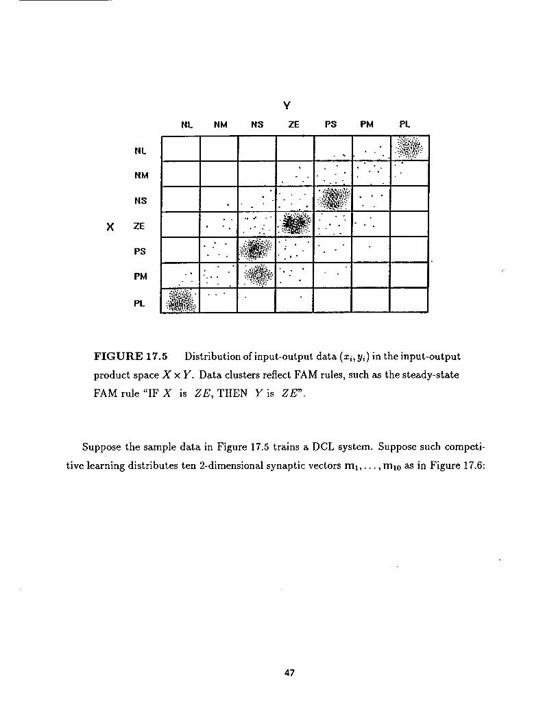
NL

NM

NS

ZE

PS

PM

PL

NL NM

• °

, •

• . .

i

NS

Y

ZE

?

;... ;..:...._:."' ' "" I. "'-.'.:

• . _

..':;_._ 'r.

:.,:'.>."i".":..-• '

PS PM

• . |

PL

|

• D

I

FIGURE 17.5 Distribution of input-output data (xi, Yi) in the input-output

product space X × Y. Data clusters reflect FAM rules, such as the steady-state

FAM rule "IF X is ZE, THEN Y is ZE".

Suppose the sample data in Figure 17.5 trains a DCL system. Suppose such competi-

tive learning distributes ten 2-dimensional synaptic vectors ml,..., mm as ill Figure 17.6:

47

×

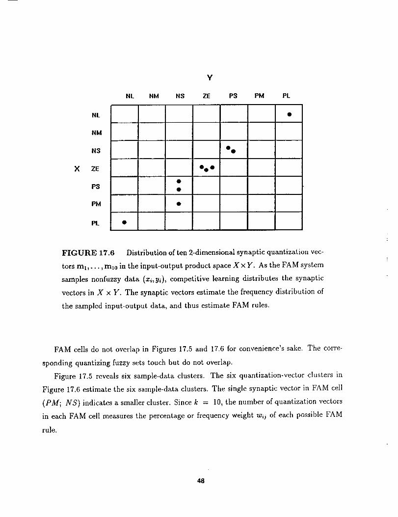
NL

NM

NS

ZE

PS

PM

PL

Y

NL NM NS ZE PS PM PL

o@ •

° o

FIGURE 17.6 Distribution of ten 2-dimensional synaptic quantization vec-

tors mx, -.., rex0 in the input-output product space X x Y. As the FAM system

samples nonfuzzy data (xi, yi), competitive learning distributes the synaptic

vectors in X x Y. The synaptic vectors estimate the frequency distribution of

the sampled input-output data, and thus estimate FAM rules.

FAM cells do not overlap in Figures 17.5 and 17.6 for convenience's sake. The corre-

sponding quantizing fuzzy sets touch but do not overlap.

Figure 17.5 reveals six sample-data clusters. The six quantization-vector clusters in

Figure 17.6 estimate the six sample-data clusters. The single synaptic vector in FAM cell

(PM; NS) indicates a smaller cluster. Since k = 10, the number of quantization vectors

in each FAM cell measures the percentage or frequency weight wij of each possible FAM

rule.

48

In general the additive combination rule (17) does not require normalizing the quantization-

vector count kij. wij = kij is acceptable. This holds for both maximum-membership de-

fuzzification (18) and fuzzy centroid defuzzification (19). These defuzzification schemes

prohibit only negative weight values.

The ten quantization vectors in Figure 17.6 estimate at most six FAM rules. From most

to least frequent or "important", the FAM rules are (ZE; ZE), (PS; NS), (NS; PS),

(PM; NS), (PL; NL), and (NL; PL). These FAM rules suggest that fuzzy variable X is

an error variable or an error velocity variable since the steady-state FAM rule (ZE; ZE) is

most important. If we sample a system only in steady-state equilibrium, we will estimate

only the steady-state FAM rule. We can accurately estimate the FAM system's global

behavior only if we representatively sample the system's input-output behavior.

The "corner" FAM rules (PL; NL) and (NL; PL) may be more importafit than their

frequencies suggest. The boundary sets Negative Large (NL) and Positive Large (PL)

are usually defined as ramp functions, as negatively and positively sloped lines. NL and

PL alone cover the important end-point regions of the universe of discourse X. They give

rnNL(x) = rnpL(x) = 1 only if x is at or near the end-point of X, since NL and PL are

ramp functions not trapezoids. NL and PL cover these end-point regions "briefly". Their

corresponding FAM ceils tend to be smaller than the other FAM ceils. The end-point

regions must be covered in most control problems, especially error nulling problems like

stabilizing an inverted pendulum. The user can weight these FAM-cell counts more highly,

for instance wit = c k_j for scaling constant c > 0. Or the user can simply include these

end-point FAM rules in every operative FAM bank.

Most FAM cells do not generate FAM rules. More accurately, we estimate every possible

FAM rule but usually with zero or near-zero frequency weight w/j. For large numbers of

multiple FAM-rule antecedents, system input-output data streams through comparatively

few FAM cells. Structured trajectories in X x Y are few.

A FAM-rule's mapping structure also limits the number of estimated FAM rules. A

FAM rule maps fuzzy sets in I" or F(2 x) to fuzzy sets in I p or F(2r). A fuzzy associative

memory maps every domain fuzzy set A to a unique range fuzzy set B. Fuzzy set A cannot

map to multiple fuzzy sets B, B', B", and so on. We write tile FAM rule as (A; /9) not

49

(A; B or B' or B" or ,..). So we estimate at most one rule per FAM-cell row in Figure

17.6.

If two FAM cells in a row are equally and highly frequent, we can pick arbitrarily either

FAM rule to include in the FAM bank. This occurs infrequently but can occur. In principle

we could estimate the FAM rule as a compound FAM rule with a disjunctive consequent.

The simplest strategy picks only the highest frequency FAM cell per row.

The user can estimate FAM rules without counting the quantization vectors in each

FAM cell. There may be too many FAM cells to search at each estimation iteration.

The user never need examine FAM cells. Instead the user checks the synaptic vector

components rnij. The user defines in advance fuzzy-set intervals, such as [1NC, UNL] for

NL. If bvL < rnij < UNL, then the FAM-antecedent reads "IF X is NL."

Suppose the input and output spaces X and Y are the same, the real interval [-35, 35].

Suppose we partition X and Y into the same seven disjoint fuzzy sets:

NL = [-35,-25]

NM = [-25,-151

NS = [-15,-5]

ZE = [-5, 5]

PS = [5, 15]

PM = [15, 25]

PL = [25, 35]

Then the observed synaptic vector mj = [9, -10] increases the count of FAM cell

PS × NS and increases the weight of FAM rule "IF X is PS, THEN Y is NS."

This amounts to nearest-neighbor classification of synaptic quantization vectors. We

assign quantization vector mk to FAM cell Fij iff mk is closer to the centroid of Fij than

to all other FAM-cell centrolds. We break ties arbitrarily. Centroid classification allows

the FAM cells to overlap.

5O

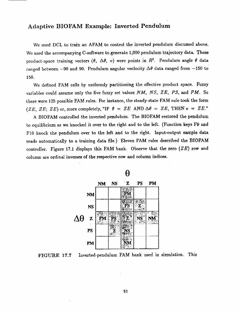
Adaptive BIOFAM Example: Inverted Pendulum

We used DCL to train an AFAM to control the inverted pendulum discussed above.

We used the accompanying C-software to generate 1,000 pendulum trajectory data. These

product-space training vectors (0, A0, v) were points in R 3. Pendulum angle 0 data

ranged between -90 and 90. Pendulum angular veclocity A0 data ranged from -150 to

150.

We defined FAM cells by uniformly partitioning the effective product space. Fuzzy

variables could assume only the five fuzzy set values NM, NS, ZE, PS, and PM. So

there were 125 possible FAM rules. For instance, the steady-state FAM rule took the form

(ZE, ZE; ZE)or, more completely, "IF 0 = ZE AND A0 = ZE, THEN v = ZE."

A BIOFAM controlled the inverted pendulum. The BIOFAM restored the pendulum

to equilibrium as we knocked it over to the right and to the left. (Function keys F9 and

F10 knock the pendulum over to the left and to the right. Input-output sample data

reads automatically to a training data file.) Eleven FAM rules described the BIOFAM

controller. Figure 17.1 displays this FAM bank. Observe that the zero (ZE) row and

column are ordinal inverses of the respective row and column indices.

FIGURE 17.7

0NM NS ' Z PS PM

_ _: ._;_;

PS i£Z _:NS_:

PM i'i'._Mi

Inverted-pendulum FAM bank used in simulation. This

51

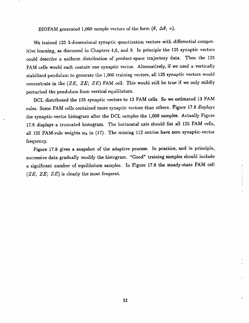
BIOFAM generated 1,000 sample vectors of the form (0, A0, v).

We trained 125 3-dimensional synaptic quantization vectors with differential compet-

itive learning, as discussed in Chapters 4,6, and 9. In principle the 125 synaptic vectors

could describe a uniform distribution of product-space trajectory data. Then the 125

FAM cells would each contain one synaptic vector. Alternatively, if we used a vertically

stabilized pendulum to generate the 1,000 training vectors, all 125 synaptic vectors would

concentrate in the (ZE, ZE; ZE) FAM cell. This would still be true if we only mildly

perturbed the pendulum from vertical equilibrium.

DCL distributed the 125 synaptic vectors to 13 FAM cells. So we estimated 13 FAM

rules. Some FAM cells contained more synaptic vectors than others. Figure 17.8 displays

the synaptic-vector histogram after the DCL samples the 1,000 samples. Actually Figure

17.8 displays a truncated histogram.

all 125 FAM-rule weights wk in (17).

frequency.

The horizontal axis should list all 125 FAM cells,

The missing 112 entries have zero synaptic-vector

Figure 17.8 gives a snapshot of the adaptive process. In practice, and in principle,

successive data gradually modify the histogram. "Good" training samples should include

a significant number of equilibrium samples. In Figure 17.8 the steady-state FAM cell

(ZE, ZE; ZE) is clearly the most frequent.

52

03 8 g 10 1| 12 13 14 15 16 17 18 23

FIGURE 17.8 Synaptic-vector histogram. Differential competitive learn-

ing allocated 125 3-dimensional synaptic vectors to the 125 FAM cells. Here

the adaptive system has sampled 1,000 representative pendulum-control data.

DCL allocates the synaptic vectors to only 13 FAM cells. The steady-state

FAM cell (ZE, ZE; ZE) is most frequent.

Figure 17.9 displays the DCL-estimated FAM bank. The product-space clustering

method rapidly recovered the 11 original FAM rules. It also estimated the two additional

FAM rules (PS, NM; ZE) and (NS, PM; ZE), which did not affect the BIOFAM

system's performance. The estimated FAM bank defined a BIOFAM, with all 13 FAM-

rule weights set wk equal to unity, that controlled the pendulum as well as the original

BIOFAM did.

53

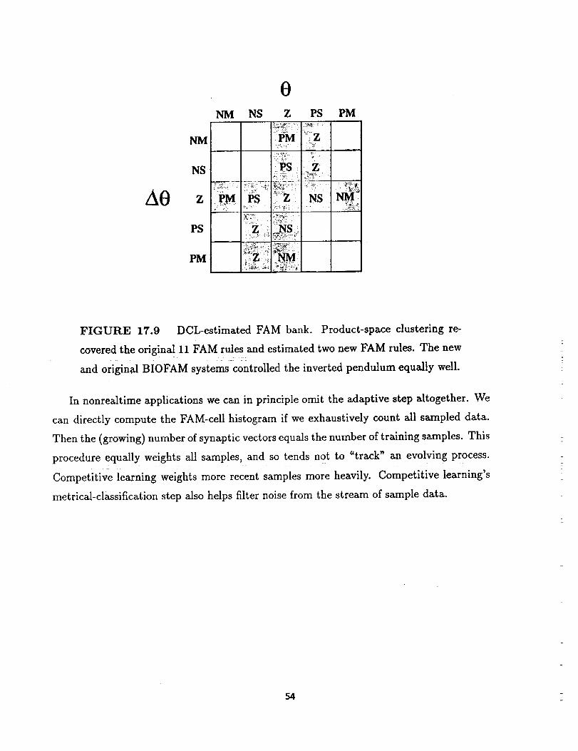
NM

NS

AO z

PS

PM

NM NS

0Z PS

!PM ;_:i;:z

P,M PS ::z i NS

i:_Z ::i _M

PM

FIGURE 17.9 DOL-estimated FAM bank. Product-space clustering re-

covered the original 11 FAM rules and estimated two new FAM rules. The new

and original BIOFAM systems controlled the inverted pendulum equally well.

In nonrealtime applications we can in principle omit the adaptive step altogether. We

can directly compute the FAM-cell histogram if we exhaustively count all sampled data.

Then the (growing) number of synaptic vectors equals the number of training samples. This

procedure equally weights all samples, and so tends not to "track" an evob(ing process.

Competitive learning weights more recent samples more heavily. Competitive learning's

metrical-classification step also helps filter noise from the stream of sample data.

54

REFERENCES

Dubois, D., Prade, H., Fuzzy Sets and Systems: Theory and Applications, Academic Press,

New York, 1980.

Hebb, D. The Organization of Behavior, Wiley, 1949.

Klir, G.J., Foger, T.A., Fuzzy Sets, Uncertainty, and Information, Prentice-Hall, 1988.

Kosko, B., "Fuzzy Knowledge Combination," International Journal of Intelligent Systems,

vol. 1,293 - 320, 1986.

Kosko, B., "Fuzzy Associative Memories," Fuzzy Expert Systems, A. Kandel (ed.), Addison-

Wesiey, in press, December 1986.

Kosko, B., "Fuzzy Entropy and Conditioning," Information Sciences, vol. 40, 165 - 174,

1986.

Kosko, B., Foundations of Fuzzy Estimation Theory, Ph.D. dissertation, Department of

Electrical Engineering, University of California at Irvine, June 1987; Order Number 8801936,

University of Microfilms International, 300 N. Zeeb Road, Ann Arbor, Michigan 48106.

Kosko, B., "Hidden Patterns in Combined and Adaptive Knowledge Networks," Interna-

tional Journal of Approximate Reasoning, vol. 2, no. 4, 377 - 393, October 1988.

Mamdani, E.H., "Application of Fuzzy Logic to Approximate Reasoning Using Linguistic

Synthesis," IEEE Transactions on Computers, vol. C-26, no. 12, 1182 - 1191, December

1977.

55

Taber, W.R., Siegel,M.A., "Estimation of Expert WeightsUsing FuzzyCognitive Maps,"

Proceedings of the IEEE 1st International Conference on Neural Networks (ICNN-87}, vol.

II, 319 - 325, June 1987.

Taber, W.R., "Knowledge Processing with Fuzzy Cognitive Maps," Expert Systems with

AppIication_, in press, 1990.

Togai, M., Watanabe, H., "Expert System on a Chip: An Engine for Realtime Approxi-

mate Reasoning, IEEE Expert, vol. 1, no. 3, 1986.

Yamakawa, T., "A Simple Fuzzy Computer Hardware System Employing MIN & MAX

Operations," Proceedings of the Second International Fuzzy Systems Associatidn (IFSA),

Tokyo, 827 - 830, July 1987.

Yamakawa, T., "Fuzzy Microprocessors-Rule Chip and Defuzzification Chip," Proceedings

of the International Workshop on Fuzzy Systems Applications, Iizuka-88, Kyushu Institute

of Technology, 51 - 52, August 1988.

Zadeh, L.A., "A Computational Approach to Fuzzy Quantifiers in Natural Languages,"

Computers and Mathematics, vol. 9, no. 1,149 - 184, 1983.

PROBLEMS

1. Use correlation-minimum encoding to construct the FAM matrix M from the fit-

vector pair (A, 13) if A = (.6 1 .2.9) and B = (.8.3 1). Is (A,B) a bidirectional

fixed point? Pass A' = (.2.9.3.2) through M and B' = (.9.5 1) through M T.

Do the recalled fuzzy sets differ from B and A?

55

2. Repeat Problem 1 using correlation-product encoding.

3. Compute the fuzzy entropy E(M) of M in Problems 1 and 2.

4. If M = A T o B in Problem 1, find a different FAM matrix M' with greater fuzzy

entropy, E(M') > E(M), but that still gives perfect recall: A o M' = B.

Find the mazimum entropy fuzzy associative memory (MEFAM) matrix M ° such

thatA o M* = B.

5. Prove: IfM = A T o B or M = A TB,A o M = B, andA -C A',then

A'oM=B.

6. Prove: max min(ak, bk) < min( max ak, max bk).l<k_m -- l__k<m l<k_<m

7. Use truth tables to prove the two-valued propositional tautologies:

(a) [ A _ (B OR C)] ----,

(b) [A _ (B AND C)] --_

(c) [ (A OR B)------* C l

(d) [(A_C) AND(B --_C)]

[(A --_ B) OR (A ----, C)I ,

[(A----,B) AND (A--_C)! ,

[(A---, C) OR (B ---- C)l ,

---* [(A AND B) _ C]

Is the converse of (c) a tautology? Explain whether this affects BIOFAM inference.

8. BIOFAM inference. Suppose the input spaces X and Y are both [-10, 10], and the

output space Z is [-100,100]. Define five trapezoidal fuzzy sets-NL, NS, ZE, PS, PL--

on X, Y, and Z. Suppose the underlying (unknown) system transfer function is

z = z 2 - y2. State at least five FAM rules that accurately describe the system's

57

behavior. Use z = x _ - y2 to generate streams of sample data. Use BIOFAM in-

ference and fuzzy-centroid defuzzification to map input pairs (x, y) to output data z.

Plot the BIOFAM outputs and the desired outputs z. What is the arithmetic average

of the squared errors (F(x, y) - x 2 + y2)2? Divide the product space X x Y x Z

into !25 overlapping FAM cells. Estimate FAM rules from clustered system data

(x, y, z). Use these FAM rules to control the system. Evaluate the performance.

Software Problems

The following problems use the accompanying FAM software for controlling an inverted

pendulum.

1. Explain why the pendulum stabilizes in the diagonal position if the pendulum bob

mass increases to maximum and the motor current decreases slightly. The pendulum

stabilizes in the vertical position if you remove which FAM rules?

2. Oscillation results if you remove which FAM rules? The pendulum sticks in a hori-

zontal equilibrium if you remove which FAM rules?

58