I1 Introduction to rock PhYsics

Make your theory as simple as possible, but no simpler'

r

1.1 Introduction

Albeft Einstein

The sensitivity of seismic velocities to crit ical reservoir parameters, such as porosity,

lithofacies, pore fluid type, saturation, and pore pressure, has been recognized for many

years. However, the practical need to quantify seismic-to-rock-property transforms and

their uncertainties has become most critical over the past decade, with the enormous

improvement in seismic acquisit ion and processing and the need to interpret ampli-

tudes for hydrocarbon detection, reservoir characterization, and reservoir monitoring.

Discovering and understanding the seismic-to-reservoir relations has been the focus of

rock physics research.

One of our favorite examples of the need for rock physics is shown in Plate I ' l . l t

is a seismic P-P reflectivity map over a submarine fan, or turbidite system. We can

begin to interpret the image without using much rock physics, because of the striking

and recognizable shape of the f'eature. A sedimentologist would tell us that the main

f'eecler channel (indicated by the high amplitude) on the left third of the image is likely

to be massive, clean, well-sorted sand - good reservoir rock. It is likely to be cutting

through shale, shown by the low amplitudes. So we might propose that high amplitudes

correspond to good sands, while the low amplitudes are shales'

Downflow in the lobe environment, however, the story changes. Well control tells

us that on the right side of the image, the low amplitudes correspond to both shale and

clean sand - the sands are transparent. In this part ofthe image the bright spots are the

poor, shale-rich sands. So, what is going on?

We now understand many of these results in terms of the interplay of sedimentologic

and diagenetic influences. The clean sands on the left (Plate l. I ) are very slightly

cemented, causing them to have higher acoustic impedance than the shales. The clean

sands on the right are uncemented, and therefore have virtually the same impedance as

the shales. However, on the right, there are more facies associated with lower energy

2II

Introduction to rock physics

deposition, and these tend to be more poorly sorted and clay-rich. We know fiomlaboratory work and theory that poor sorting can also influence impedance. In theturbidite system in Plate l. l both the clean, slightly cemented sand and the cleanuncemented sand are oil-saturated. These sands have essentially the same porosity anclcomposition, yet they have very different seismic signatures.

This example i l lustrates the need to incorporate rock physics principles into seismicinterpretation, and reservoir geophysics in general. Despite the excellent seismicquality and wellcontrol, the correct interpretation required quantifying the connec-tion between geology and seismic data. A purely comelational approach. for instanceusing neural networks or geostatistics. would not have been so successful.

Our goal in th is f i rs t chapler is to rev iew some of ' the basic rock physics conceptsthat are crit ical fbr reservoir geophysics. Although the cliscussion is not exhaustive, weassess the strengths, weaknesses, and common pitfalls of some currently used methods,and we make specific tecommendations for seismic-to-rock-property transforms formapping of lithology, porosity, and fluids. Several of these rock physics methods aref-urther discussed and applied in Chapters 2, 3, and 5 .

-

1.2 velocity-porosity relations for mapping porosity and facies

Rock physics models that relate velocity and impedance to porosity and mineralogy(e.g. shale content) form a crit ical part of seismic analysis for porosity and lithofacies.In this section we illustrate how to recognize the appropriate velocity-porosity relationwhen approaching a new reservoir geophysics problem.

Pitfall

one of the most serious and common mistakes that we have observed in industrypractice is the use of inappropriate velocity-porosity relations for seismic mappingof porosiry and lithofacies. The most common error is to use overly stiffvelocity-porosity relarions, such as the classical empirical trends of wyll ie et at. (1956s,Raymer. Hunt. and Gardner (Ray mer et al., l9g0t, Han ( l9g6). or Raiga-Clemenceauet al. (1988), the crirical porosity model 1Nur, lt9921. or penny-shapecl crack moclels."Sonic porosity," derived from sonic logs using the wyll ie rime average, is perhapsthe worst example. Implicit in these relations is that porosity is controlled by vari-ations in diagenesis, which is not always the case. Hence, crit ical sedimentologicvariations are ignored.

Solution

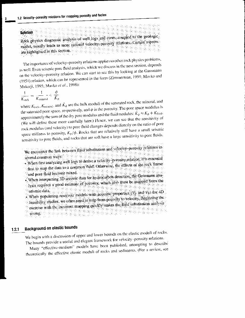
Rock physics diagnostic analysis. o[ well, logs and cores' coupled to the geologic

model, usually r.uo, tl *ore rational velocity-porosity relations' ceflain aspects

are highlighted in this section'

Theimportanceofvelocity-porosityrelationsappliestootherrockphysicsproblems'

aswel l .Evenseismicpn,"nuioanalys is ,whichwediscussinthenextsect ion,depends

on the velocity-porosity relation' We can start to see this by looking at the Gassmann

(1951) relation, whicir can be represented in the fbrm (Zimmerman' 1991; Mavko and

Mukerji, 1995; Mavko et al" 1998):

t l oKrn.k Kmincr" l K 6

1.2 Veloci$-porosi$ relations for mapping porosity and facies

where Krn.p, Krnincral' and (4 are the bulk moduli of the saturated rock' the mineral' and

-o"" mndttlus is

[1"i,ffi;;:r#", ;"il;;;, ;;o 4 is tr," porosirv rhe pore space modurus isV . >. K, -L Ko. . , , ' -

ffi :::H:::'il"'ffi iii"o,,ryJT*"11',Til'::"li:""":'l;;;[:;"f lJ"ff :;liiJ";'T ffi i I #.' *;;; *'"* ", I ater. ) He n ce' -: : ii,::: j::: jT "':il

j'Ji';"::::i;:::iJJ,'""i ".,".to)

to pore fluid changes depends directlv on the ratio or poreo cmrl l seismic

;:: J' ffi :' J ;; ;;; J; i,' u r ) o Ro c k s th at :l: :::i'1"'"'1" T:T.ffi ;,:T jl J:'Tl:::ffi:lli:'ri-tr"i;.;o ro.r, rhat are sort have a large sensitivitv to pore fluids'

1.2.1

weencounterthel inkbetweenf luidsubst i tut ionandveloci ty-porosi tyrelat ionsin

:ffi:'" i,T,T::,il[ weu rogs ro derive a velocitv-porositv relation. ir is essenrial

firsr to map the data to a common nulo. oil1l.*ira ,n.-"n".ts of the rock frame

. ffiJ""[,:;1"::'r'i"",T]J,iL o,1" ror hydrocarbon.derecrionl*::^'T:"i.":::tysis require, " r"J;;;;;;;i;"""1v'

which also must be mapped from the

. ffffifi[ating reservoir models *']l,T*"tc properties,lY:.-o vs) for 4D

feasibil i ty studies. *. oft n need.to map from porosity to velocity' Beginning the

;:*i"';ffi;;;'"ip'"s

quictrv makes the nuid substitution anarvsis

Background on elastic bounds

Webeg inw i thad i scuss iono fuppe rand lowerboundson thee las t i cmodu l i o f rocks .

Theboundsprovideausefulanclelegantframeworkforvelocity-porosityrelations'

Many. .ef f 'ect ive-medium,,modelshavebeenpubl ished,at tempt ingtodescr ibe

theo re t i ca l l y thee f tec t i vee las t i cmodu l i o f rocksandsed imen ts . (Fo ra rev iew ,see

4-

Introduction to rock physics

3 K ,

=

.zo

q

Upper bound

*n* 1,f. \\ ',fri ] stiffernoreshapes

,7-\Lower bound K2

Volume fraction of material 2

Figure 1'2 Conceptr-ral i l lustrat ion of bounds fbr the eff-ect ive elast ic bulk modLrlus of a mixture oftwo materials.

Mavko et al., 1998.) Some models approximate the rock as an elastic block of min-eral perturbed by holes. These are often ref'erred to as "inclusion models." Others tryto describe the behavior of the separate elastic grains in contact. These are sometimescalled "granular-medium models" or "contact models." Regardless of the approach, themodels generally need to specity three types of infbrmation: (1) the volume fiactionsof the various constituents, (2) the elastic moduli of the various phases, and (3) thegeometric details of how the phases are arranged relative to each other.

In practice, the geometric details of the rock and sediment have never been adequatelyincorporated into a theoretical model. Attempts always lead to approximations andsimplif ications, some better than others.

When we specify only the volume fractions of the constituents and their elasticmoduli, without geometric details of their arrangement, then we can predict only theupper and lower bounds on the moduli and velocities of the composite rock. How_ever, the elastic bounds are extremely reliable and robust, and they suffer little fromthe approximations that haunt most of the geometry-specific effective-medium moclels.Furthermore, since well logs yield infbrmation on constituents and their volume frac-tions, but relatively little about grain and pore microstructure, the bouncls turn out tobe extrernely valuable rock physics tools.

Figure 1.2 i l lustrates the concept for a simple mixture of two constltuents. Thesemight be two diff-erent minerals or a minerar plus fluid (water, oil, or gas). At any givenvolume fraction of constituents the efl'ective modulus of the mixture will fall betweenthe bounds (somewhere along the vertical dashed line in the figure), but its precise valuedepends on the geometric details. we use, for example, terms like ..stiff pore shapes,,and "sofi pore shapes" to describe the geometric variations. Stiffer grain or poreshapes cause the value to be higher within the allowable range; softer grain or poreshapes cause the value to be lower.

5-

l.2 Velocity-porosi$ relations for mapping porosity and facies

The Voigt and Reuss bounds

The simplest, but not necessarily the best, bounds are the Voigt ( 1910) and Reuss (1929)

bounds. The Voigt upper bound on the effective elastic modulus, My, of a mixture of

N mater ia l ohases is

t v t v : l f i M ii - I

wrtn

f the volume fiaction of the lth constituent

M i the elastic modulus of the lth constituent

There is no way that nature can put together a mixture of constituents (i.e., a rock) that

is elastically stiJJer than the simple arithmetic average of the constituent moduli given

by the Voigt bound. The Voigt bound is sometimes called the isostrain average, because

it gives the ratio of average stress to average strain when all constituents are assumed

to have the same strain.

The Reu.rs knver brtund of the effective elastic modulus, MB, is

( 1 . 2 )

There is no way that nature can put together a mixture of constituents that is elas-

tically softer than this harmonic average of moduli given by the Reuss bound. The

Reuss bouncl is sometimes called the i.sos/re.rs average, because it gives the ratio of

average stress to average strain when all constituents are assumed to have the same

stress.

Mathematically the M in the Voigt and Reuss fbrmulas can represent any modulus:

the bulk modulus K, the shear modulus p, Young's modulus E, etc. However, it makes

most sense to compute the Voigt and Reuss averages of only the shear modulus, M : lt,

and the bulk modulus, M : K, and then compute the other moduli from these, using

the rules of isotropic l inear elasticity.

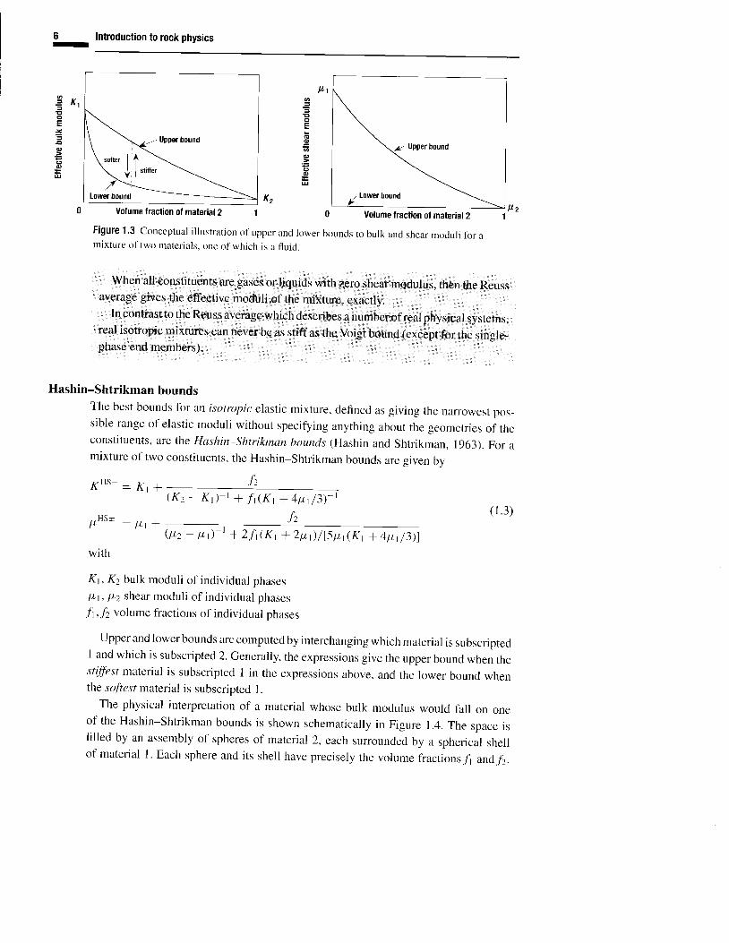
Figure 1.3 shows schematically the bounds for elastic bulk and shear moduli, when

one of the constituents is a l iquid or gas. In this case, the lower bound corresponds

to a suspension of the particles in the fluid, which is an excellent model fbr very soft

sediments at low effective stress. Note that the lower bound on shear modulus is zero,

as long as the volume tiaction of fluid is nonzero.

The Reuss average describes exactly the effective moduli of a suspension of solid

grains in a fluid. This wil l turn out to be the basis lor describing certain types ol

clastic sediments. It also describes the moduli of "shaltered" materials where solid

fragments are completely surrounded by the pore fluid.

( l . l )

r _ $ r ;M*

- l'-, M,

I

6-

Introduction to rock physics

Upper bound

softer i,lti'*. ''J,' ] smrer

v-\Lower bound

I t t

Upper bound

Lower bound

( 1 . 3 )

E x ,E

=o.=o

q

@

U

K2

Volume fiaction of material 2 1 0 Volume fraction of material 2

Figure1.3 Conceptual i l lust rat ionofupperancl lowerboundstobulkandshearmodul i lbramixture of two materials, one of which is a fluid.

When all constituents are gases or l iquids with zero shear modulus, then the Reussaverage gives the effective moduli of the mixture, exactly.

ln contrast to the Reuss average which describes a numberof real physical systems,real tsotropic mixtures can never be as stiffas the Voigr bound (except for the single-phase end members).

Hashin-Shtrikman boundsThe best bounds fot an isotropic elastic mixture, defined as giving the narrowest pos-sible range of elastic moduli without specitying anything about the geometries of theconstituents, are the Hashin-shtrikman bouncls (Hashin and Shtrikman, 1963). For amixture of two constituents, the Hashin-shtrikman bounds are siven bv

I tz

6 H S + : K 1 f

H ( +

U " ' - : l t t +

with

.fz( K z - K t ) ' + f t ( K t + 4 t t t 1 3 ) l

fz.( t t z - t t ) ' +2 f tK t +2pr ) / l5pr (Kr + 4pr l3 ) l

Kt, Kz bulk moduli of individual phases

l.Lt, tL2 shear moduli of individual phases

.fl,/2 volume fiactions of individual phases

Upper and lower bounds are computed by interchanging which material is subscriptedI and which is subscripted 2. Generally, the expressions give the upper bound when thestiffbst material is subscripted I in the expressions above, and the lower bound whenthe softest material is subscripted I .

The physical interpretation of a material whose bulk modulus would fall on oneof the Hashin-shtrikman bounds is shown schematically in Figure 1.4. The space isfilled by an assembly of spheres of material 2, each surrounded by a spherical shellof material l. Each sphere ancl its shelr have precisely the volume fractions.ll andf2.

E

a

7-

1.2 Veloci$-porosity relations for mapping porosity and facies

Figure 1.4 Physical interpreration of the Hashin-Shtrikman bounds for bulk modulus of a

two-phase material.

The upper bound is realized when the stiffer material forms the shell; the lower bound,

when it is in the core.

A more general form of the Hashin-shtrikman bounds, which can be applied to more

than two phases (Berryman, 1995), can be written as

l

I

. l

I

l{j

IIjI)

I

I

KHS+ - A(Fn,"^), KHS- : A(trmin)

pHS+ - f((K-u^, 4n'o*)), FHS- : f(((K.in, l 'n' i"))

where

t r \ ' 4\ ( - ) - l - - ) - - -

\ x t r t - 4 z l 3 l 3 -

I t \ - lf ( : ) : ( _ ) - :

\ / l ( r ) + z /

u / 9 K + 8 \1 ( K . t r \ : ; l - : J l6 \ h l 2 1 t /

( 1 .4 )

The brackets (.) indicate an average over the medium, which is the same as an average

over the constituents, weighted by their volume fractions.

The separation between the upper and lower bounds (Voigt-Reuss or Hashin-

Shtrikman) depends on how elastically diflerent the constituents are. As shown in

Figure 1.5, the bounds are ofien tairly similar when mixing solids, since the elastic

moduli of common minerals are usually within a factor of two of each other. Since

many ef-fective-medium moclels (e.g., Biot, 1956; Gassmann, 195 l; Kuster and Toksciz'

1974) assume a homogeneous mineral modulus, it is often useful (and adequate) to

represent a mixed mineralogy with an "average mineral" modulus, equal either to one

of the bounds computed for the mix of minerals or to their average (,yus+ + MHS-) 12.

Calcite + dolomite

Upperbound

Lowerbound

8-

lntroduction to rock physics

Calcite + water

Upperbound

0.4 0.6 0.8Porosity

Figure 1'5 on the left, a mixturc of two minerals. The upper and lower bounds are close when theconstituents are elastically similar. On the right, a mixture of mineral and wlter. The upper andlower bolrnds are lar apart when the constituents are elastically diff-erent.

On the other hand, when the constituents are quite dit l 'erent - such as minerals and porefluids - then the bounds become quite separated, and we lose some of the predictivevalue.

80

70

9 6 0

* u oE + o! 3 0E- 2 0

t 0

0

77

76

a 7 5

? , 0E z ri 7 2E' 7 1

70

69

0.2 0.4 0.6 0.8 1 0 o.2Fraction of dolomite

Nole that when pr,n;n : 0. then KHS- is the same as the Reuss bound. In this case,the Reuss or Hashin-shtrikman lower bounds describe exacrly the moduli of asuspension of grains in a pore ffuid. These also describe the moduli of a mixture offluids and/or gases.

1.2.2 Generalized velocity-porosity models for clastics

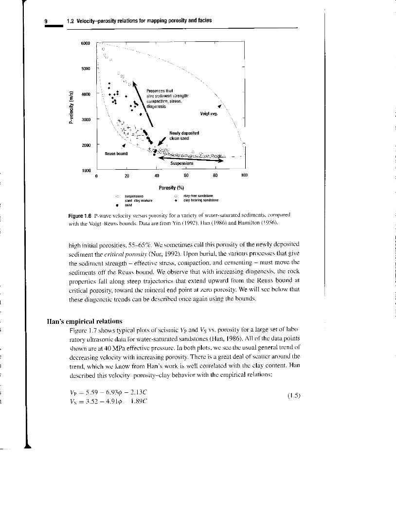
Brief "life story" of a clastic sedimentThe bounds provide a framework for understanding the acoustic properties of sediments.Figure 1.6 shows P-wave velocity versus porosity fbr a variety of water-saturated sedi-ments, ranging from ocean-bottom suspensions to consolidated sandstones. The Voigtand Reuss bounds, computed for mixtures of quartz and water, are shown fbr compar-ison. (Strictly speaking, the bounds describe the allowable range for elastic moduli.When the corresponding P- and S-wave velocities are derived from these moduli. it iscommon to refer to them as the "upper and l0wer bounds on velocity.")

Befbre deposition, sediments exist as particles suspended in water (or air). As such.their acoustic properties must fall on the Reuss average of mineral and fluid. When thesediments are first deposited on the water bottom, we expect theirproperties still to lie on(or near) the Reuss average, as long as they are weak and unconsoliclated. Their porositlposition along the Reuss average is determined by the geometry of the particle packingClean' well-sorted sands wil l be deposited with porositi esnear 40To.poorly sorted sandswill be deposited along the Reuss average at lower porosities. Chalks wil l be deposited a

I-

1.2 Velocity-porosity relations for mapping porosity and facies

r a

, a

, o o !r ar . l

o8 c

a

Processes lhatgive sediment strength:coffpaction. slress.diagenesis J \ ,/ \

Voigt avg.

. t

\ ' ir+at':S- , t Newlydeposited

. \ / c leansand

+ i6qReuss bound

Porosity (%)

o suspensions o clay-lree sandstone

: ::l:*or rotre . clav-bearinq sandstone

Figure 1.6 P-wave velocity versus porosity fbr a variety of water-saturated sedirnents, compared

with the Voigt,Reuss bor.rnds. Data are fiom Yin (1992), Han (1986) and Hamilton (1956).

high init ial porosiries, 55-65Vo. We sometimes call this porosity of the newly deposited

sediment the critical porosit), (Nur, 1992). Upon burial, the various processes that give

the sediment strength - efl'ective stress, compaction, and cementing - must move the

sediments off the Reuss bound. We observe that with increasing diagenesis, the rock

properties fall along steep trajectories that extend upward from the Reuss bound at

critical porosity, toward the mineral end point at zero porosity. We will see below that

these diagenetic trends can be described once again using the bounds.

llan's empirical relations

Figure L7 shows typical plots of seismic Vp and V5 vs. porosity for a large set of labo-

ratory ultrasonic data for water-saturated sandstones (Han, 1986). All of the data points

shown are at 40 MPa effective pressure. In both plots, we see the usual general trend of

decreasing velocity with increasing porosity. There is a great deal of scatter around the

trencl, which we know from Han's work is well correlated with the clay content. Han

described this velocity-porosity-clay behavior with the empirical relations:

V p : 5 . - 5 9 - 6 . 9 3 0 - 2 . 1 3 CV s : 3 . 5 2 - 4 . 9 1 0 - 1 . 8 9 C

( 1 . 5 )

A 4oooE

'6

6? 3ooo

10 Introduction to rock physicsr

GE +.s5s'

4

Euitding sandstonep-sand$tone

Gull saddstoneClean sandstone

. Tight gas sandstone

a .o o o

I

. r t ". r | ^ . . . tr o f .

^ i ^

. . ^r j l

0 0.05 0.1 0.15 0.2 0.25 0.3 0.35

Porosity

o l o ' r

. Buitding sandstoner P-sandstone

Gulf sandslonex Clean sandstone. Tight gas sandstone

r . ^t a a

a ^ ^

t

, a

t a a a

a

3o

!

g 2.5

1 .50 0.05 0.1 0.15 0.2 0.25 0.3 0.35

Porosity

Figure 1.7 Velocity versus porosity fbr water-saturated sandstones at 40MPa. Data are ultrasonicmeasurements fiom Han (1986).

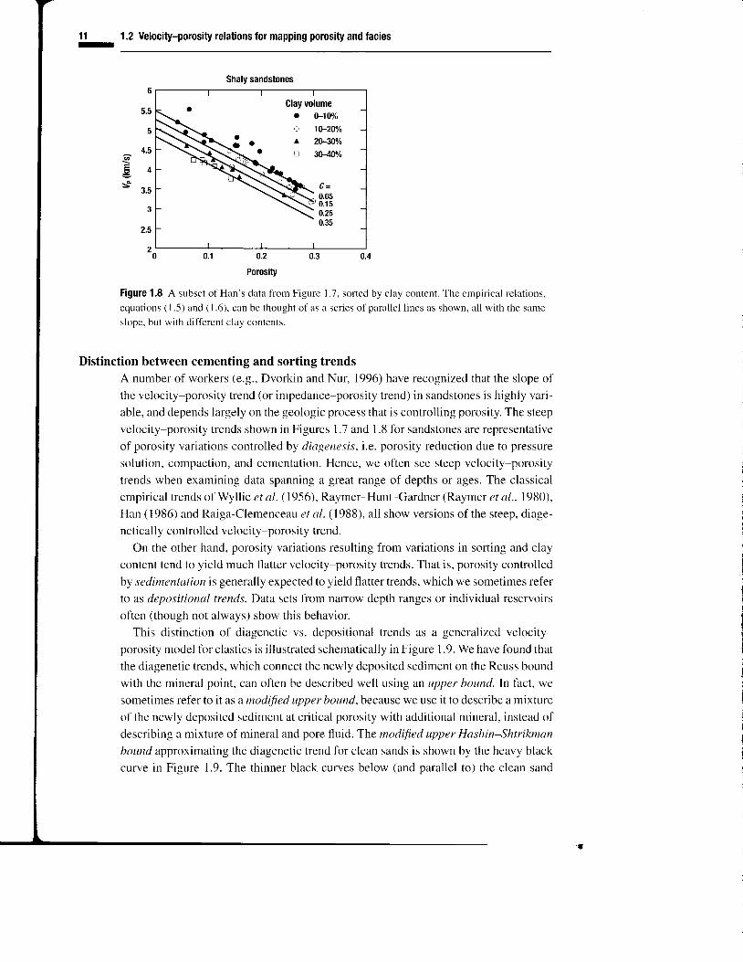
where the velocities are in km/s, @ is the porosity, and C is the clay volume fraction.These relations can be rewritten sliehtlv in the form

vp : (5.59 - 2.13C) - 6.930v q : ( 3 . 5 2 - 1 . 8 9 C ) - 4 . 9 1 0 ( l 6 )

which can be thought of as a series of parallel velocity-porosity trends, whose zero-porosity intercepts depend on the clay content. These contours ofconstant clay contentare illustrated in Figure 1.8, and are essentially the steep diagenetic trends mentionedin Figure 1.6. Han's clean (clay-free) l ine mimics the diagenetic trend for clean sands,while Han's more clay-rich contours mimic the diagenetic trends fbr dirt ier sands.Vernik and Nur (1992) and Vernik (1997) found similar velocity-porosity relations, andwere able to interpret the Han-type contours in terms of petrophysical classificationsof sil iciclastics. Klimentos (1991) also obtained similar empirical relations betweenvelocity, porosity, clay content and permeability for sandstones.

As with any empirical relarions, equarions (1.5) and (1.6) are mosr meaningful forthe data from which they were derived. It is dangerous to exlrapolate rhem to othersituations. although the concepts that porosity and clay have large impacts on p- andS-wave velocities are quite general for clastic rocks.

When using relations l ike these, it is very imponant to consider the coupled effectsof porosity and clay. If two rocks have the same porosily. but different amounts ofclay, then chances are good that the high clay rock has lower velocity. But if porositydecreases as clay volume increases. then the high clay rock mighr have a highervefoc i ty . (See a lso Sect ion 2.2.3. )

Glay volume. |e"IOVo

a 1|F20%^ 2W30%tr 3(F40%

1 1I

1.2 Velocity-porosity relations for mapping porosity and facies

0 0.1 0.2 0.3 0.4

Porosity

Figure 1,8 A subset of Han's data frorn Figure 1.7, sorted by clay content. The empirical relations,

equations ( I .5) and ( I .6), can be thought of as a series of parallel lines as shown, all with the same

slope, but with different clay contents.

Distinction between cementing and sorting trends

A number of workers (e.g., Dvorkin and Nur, 1996) have recognized that the slope of

the velocity-porosity trend (or impedance-porosity trend) in sandstones is highly vari-

able, and depends largely on the geologic process that is controlling porosity. The steep

velocity-porosity trends shown in Figures 1.7 and 1.8 fbr sandstones are representative

of porosity variations controlled by diagenesi.s, i.e. porosity reduction due to pressure

solution, compaction, and cementation. Hence, we often see steep velocity-porosity

trends when examining data spanning a great range of depths or ages. The classical

empirical trends of Wyllie et al. ( 1956), Raymer-Hunt-Gardner (Raymer et al., 1980),

Han ( 1986) and Raiga-Clemenceau et al. (1988), all show versions of the steep, diage-

netically controlled velocity-porosity trend.

On the other hand, porosity variations resulting from variations in sorting and clay

content tend to yield much flatter velocity-porosity trends. That is, porosity controlled

by sedimentaliorz is generally expected to yield flatter trends, which we sometimes refer

to as depositional trends. Data sets from narrow depth ranges or individual reservoirs

often (though not always) show this behavior.

This distinction of diagenetic vs. depositional trends as a generalized velocity-

porosity model for clastics is illustrated schematically in Figure 1.9. We have found that

the diagenetic trends, which connect the newly deposited sediment on the Reuss bound

with the mineral point, can often be described well using an upper bound. In fact, we

sometimes ref'er to it as a modified upper bound, because we use it to describe a mixture

of the newly deposited sediment at critical porosity with additional mineral, instead of

describing a mixture of mineral and pore fluid. The modified upper Hashin-Shtrikman

bound approximating the diagenetic trend for clean sands is shown by the heavy black

curve in Figure 1.9. The thinner black curves below (and parallel to) the clean sand

G

S . 43.5

2.5

2

12 Introduction to rock physicsr

5500

Diagenetic vs. sorting trends

a- Mineral pornl

Clean sand\ diaoenetic

\\ tieno

\

4000

s 3500

3000

2500

2000

1 500

1 0000.50 .30 .2

Porosity

Figure 1.9 General ized clast ic modcl. Sediments are deposited along the suspension l ine. Clean,well-sorted sands wil l have init ial (cr i t ical) porosity oi-0.4. Poorly sorted sediments wil l have asmaller cr i t ical porosity. Burial, compaction and diagenesis move data off the suspension l ine.

Sediments of constant shal iness or sort ing and variable age (or degree of diagenesis) lal l along the(black) cenrenting trends. Sedirrrents ofconstant age but variable shatl iness or sort ing wil l tal l alongthe (gray) sorting trends.

line represent the diagenetic trends fbr more clay-rich sands. They are computed agair

using the Hashin-Shtrikman upper bound, connecting the lower critical porosities fbl

more clay-rich sands with the elastically softer mineral moduli for quartz-clay mix

tures. These paral lel trends are essential ly the same as Han's empir ical l ines, shown ir

Figure 1.8.

We observe empirically that the modified upper Hashin-Shtrikman bound describes

fairly well lhe variation ol velocity with porosity during compaction and diagenesis of

sandstones. While it is diff icult to derive from first principles, a heuristic argument for

the result is that diagenesis is the stiffest way to mix a young sediment with additional

mineral (i.e.. the stiffest way to reduce porosity); an upper bound describes the stif lest

way to mix two constituents.

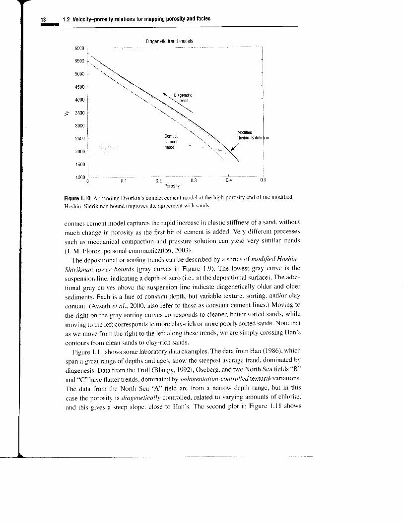
A slight improvement over the modified upper Hashin-Shtrikman bound as a diag

netic trend for sands can be obtained by steepening the high-porosity end. An eff'ecti

way to do this is to append Dvorkin's model (Dvorkin and Nur, 1996) for cemet

ing of grain contacts, as i l lustrated in Figure l. l0 (discussed more in Chapter 2). T

1 3I

1.2 Velocity-porosi$ relations for mapping porosity and facies

Diagenetic trend models6 0 0 0 ' ' T i " '

4500

4000

3500

2000

PorositY

Figure 1 ,10 Appending Dvorkin's contlct cement model trt the high-porosity end o1' the modified

Hashin-shtrikman bound intproves the agreement with sands.

contact-cement model captures the rapid increase in elastic stiffness of a sand, without

much change in porosity as the first bit of cement is added. Very difl'erent processes

such as mechanical compaction and pressure solution can yield very similar trends

(J. M. Florez, personal communication. 2003).

The depositional or sorting trends can be described by a series of modified Hashin

Shtrikmun lovter bounds (gray curves in Figure L9). The lowest gray curve is the

suspension l ine, indicating a depth of zero (i.e., at the depositional surface). The addi-

tional gray curves above the suspension l ine indicate diagenetically older and older

sediments. Each is a line of constant depth, but variable texture, sorting, and/or clay

content. (Avseth et al.,20OO, also ref'er to these as constant cement l ines.) Moving tt l

the right on the gray sorting curves corresponds to cleaner, better sorted sands, while

moving to the left corresponds to more clay-rich or more poorly sorted sands. Note that

as we move from the right to the left along these trends, we are simply crossing Han's

contours fiom clean sands to clay-rich sands.

Figure I . l I shows some laboratory data examples. The data from Han ( 1986)' which

span a great range of depths and ages, show the steepest average trend, dominated by

cliagenesis. Data fiom the Troll (Blangy, 1992), Oseberg, and two North Sea fields "B"

and "C" have flatter trends, dominated by sedimentation-controlled textural variations.

The data from the North Sea 'A" field are from a nalrow depth range, but in this

case the porosity is diagenetically controlled, related to varying amounts of chlorite,

and this gives a steep slope, close to Han's. The second plot in Figure l. l I shows

1 500

0.50.40 .20 .1

Diagenetic

14 lntroduction to rock physics-

Yp-porosity trends

. Gulf of Mexrco (Han)

0 0.05 0.1 0.15 0.2 0.25 0.3 0.35 0.4Porosity

Sorting vs. cementing trends

5 km. old sands

l'' rssltx

"*-*__**:

0 0.05 0.1 0.15 0.2 0.25 0.3 0.35 0.4Porosity

4

s ' 3

2

1

0

Figure 1.11 Left: Trends in yp versus porosity, showing a broad range ofbehaviors. Steep trends(Han; N. Sea A) are dominated by diagenesis. Flatter trends are dominated by textural variations.

Right: Another comparison of llelds showing the difference between diagenetic trends and

sedimentological trends.

another comparison of North Sea fields showing the difference between diagenetic

trends and depositional trends. In both cases, the data are from fairly narow depth

ranges.

More detailed theory and applications of various rock physics models for character-

ization of sand-shale systems are presented in Chapter 2.

Porosity has an enormous impacl on P- and S-wave velocities.. Usual ly, an increase in porosity wi I I result in a decrease of P- and S-wave velocities.

Often the correlation is good, allowing porosity to be estimated from impedance.. For sandstones. clay causes scalter around the velocity-porosity trend. although

data grouped by nearly constant clay sometimes yield systematic and somewhat

parallel trends (Figure 1.8). In consolidated sandstone$, clay tends to decrease

velocity and increase VplVsratio.ln unconsolidated sands, clay sometimes slightly

stiffens the rock.. Variations in pore shape also cause variable velocity-porosily trends. This is usually

modeled in terms of round vs. crack-like aspect ratio for pores. We now understand

that deposition-controlled textural variations, such as sorting, lead to specific,

similar variations in clastics. Increasing clay and poorer sofling act roughly in

the direction of smaller aspect ratios.. Popular rela{ions. l ike those of Han ( 1986). Wyll ie et al. (195$,and Raymer el a1.

(1980), describe steep velocity*porosity trends (as in Figure 1.6), which. when

correct. indicate conditions that are fiavorable for mapping porosity from velocity.

15 1 ,3I

Fluid substitution analysis

These are only appropriate when porosity is controiled by diagenesis. often seenovergreat depth ranges. These relations can be misleading for understanding lateralvariations of velocity within narrow depth ranges. They should cer-tainly never beused for f luid substiturion analysis.

. we expect very shallow velocity-porosity trends when porosity varies texturally,because of sorting and clay contenf. These trends, when appropriate, indicateconditions where mapping porosity from velocity is diff icult. However, these tex-rurally controlled rocks tend to be elastically sofrer and have a larger sensitivity

::u:o,::.Ou'0,

and pore pressffe. and rhese characrerisrics are advanrageous for 4D

1.3 Fluid substitution analysis

This section lbcuses on fluid substitution, which is the rock physics problem of under-standing and predicting how seismic velocity and impedance depend on pore fluids.At the heart of the fluid substitution problem are Gassmann's (195 l) relations, whichpredict how the rock modulus changes with a change of pore fluids.

For the fluid substitution problem there are two fluid efTects that must be considered:the change in rock bulk density, and the change in rock compressibility. The com-pressibility of a dry rock (reciprocal of the rock bulk modulus) can be expressed quitegenerally as the sum of the mineral compressibil i ty and an extra compressibil i ty dueto the pore space:

( 1 . 7 )

where @ is the porosity, Ka.y is the dry rock bulk modulus, Kminerar is the mineral bulkmodulus, and Kq is the pore space stiffness defined by:

yf Vporc

iJ ltpore

do( 1 . 8 )

Here, vpo.e is the pore volume, and o is the increment of hydrostatic conlining stresstiom the passing wave. Poorly consolidated rocks, rocks with microcracks. and rocksat low effective pressure are generally soft and compressible and have a small K4.Stiff rocks that are well cemented, lacking microcracks, or at high effective pressurehave a large K4. In terms of the popular but idealized ellipsoidal crack models, low-aspect-ratio cracks have small K4 and rounder large-aspect-ratio pores have large K4.In simple terms we can write approximate\y Kq x oKmineral where cy is aspect ratio.(This approximation is best at low porosity.)

16 lntroduction to rock physics-I

.==vv

Porosity

Figure 1.12 Norrr-ralized rock bulk modulus versus porosity, with contours of constant pore spacestifTness. Points A and B con'espond kl two difl'erent dry rocks at the same porosity. Points A' and B'are the corresponding water-saturatcd values. The sensitivity to fluid changes is proportional to thecontour spacing.

Similarly, the compressibi l i ty of a soturated rock can be expressed as

t tI

K'* -

1(",^- - a

K 4, I K nuiaKnineral/Kminerat - Kflui.t( l e l

( l . r i )

or approximately as

l t a: _ t _

K.u r K r i r r c . r l K * - lK11a i , 1

where Ksu;.1 is the pore-fluid bulk modulus. Comparing equations ( I .7) and ( L 10), wrcan see that changing the pore fluid has the eff'ect of changing the pore-space stiffnessFrom equation (1.10) we see also the well-known result that a stiff rock, with largpore-space stiflhess Ka, will have a small sensitivity to fluids, and a soft rock, witsmall K4, wil l have a larger sensitivity to fluids.

Figure 1.12 shows a plot of normalized rock bulk modulus K/K,,, ir"rut versus poroiity (where K : Ksat or K,r,y) computed for various values of normalized pore-spacstiffness K4 f K,,,,'erat.Since K4 and K11u;,t always appear added together (as in equatio(1.10)), then fluid substitution can be thought of as computing the change L(KaKnuio): AKnui,r and jumping the appropriate number of contours in the graph. Frthe contour interval in Figure 1.12, the difference between a dry rock and a watesaturated rock is three contours, anywhere in the plot. For the example shown, tlstarting point A was one of Han's ( 1986) dry sandstone data points, with effective d

B ) \ - , - - ----.

KolKnt -0 .1 -

0

17 1,3 Fluid substitution analysisI

rock buf k modulus K,try/Kn,in..ul :0.44 and porosity Q:0.20. To saturate, we move upthe amount LKnuiaf K-,nerat :0.06, or three contours. The water-saturated ntodulus canbe read off directly as K,rt/Krin.,ar:0.52, point A'. The second example shown (points

B-B') is for the same two pore fluids and the same porosity. However, the change inrock stiffness during fluid substitution is much larger.

Pitfall

Seismic sensitivity to pore fluids is not uniquely,relared to porosity.

Solution

seismic ffuid sensitivity is determined by a combinarion of porosity and pore-spacestiffness. A softer rock wil l have a larger sensitivity to fluid substirudon than a stiff lerrock al the same porosity. On Figure l. 12. we can see l-hat regions where the contoursare far apart wil l have a large sensitivity to fluids. and regions where the contours are

il:::;;:five a small sensitivity. Gassmann's relarions simply and retiabty describe

Equat ions (1.7) and (1.9) together are equivalent to Gassmann's (1951) re lat ions. I fwe algebraically eliminate K4 from equations (1.7) and (1.9) we can write one of themore familiar but less intuit ive forms:

K,,, Kory Knri,t( 1 . 1 r )

Krnineral - Kro, Kmineral - Kory

and the companion result

Fsat : Fdry

+d(Kmin..nt - Knuia)

( 1 . 1 2 )

Gassmann ' sequa t i ons (1 .11 )and (1 .12 )p red i c t t ha t f o ran i so t rop i c rock , t he rockbu l k

modulns wil l change if the fluid changes, but the rock shear modulus wil l not.These dry and saturated moduli, in turn, are related to P-wave velocity Vp :

trTtrTTlRldn and S-wave velocity Vs : nl1t/j,where p is the bulk density givenby

P: QPnu i , t + ( l - d )Pn ' ,n . r r t ( r . 1 3 )

In equations (1.7)-(l. l l), d is normally interpreted as the rotal porosity, although inshaly sands the proper choice of porosity is not clear. We sometimes find a better fit tofield observations when eflective porosity is used instead. The uncertainty stems fromGassmann's assumption that the rock is monomineralic, in which case the porosity isunambiguously all the space not occupied by rnineral. Clay-rich sandstones actually

18 Introduction to rock physicsn

violate the monomineralic assumption, so we end up forcing the Gassmann relations

to apply by adapting the porosity and/or the effective mineral properties. Should the

clay be considered part of the mineral frame'l If so, does the bound water inside the

clay communicate sufficiently with the other fiee pore fluids to satisfy Gassmann's

assumption of equilibrated pore-fluid pressure, or should the bound water be considered

part of the mineral fiame? Alternatively, should the clay be considered part of the pore

fluid'? If so, then the functional Gassmann porosity is actually larger than the totalporosity, but the pore fluid should be considered a muddy suspension containing clay

particles.

1.3.1 The Gassmann fluid substitution recipe

The most common scenario is to begin with an init ial set of velocities and densities,yJ", yJ

", and p( r) corresponding to the rock with an init ial set of f luids, which we call"f luid 1." These velocities often come from well logs, but might also be the result of

an inversion or theoretical model. Then fluid substitution is perfbrmed as fbllows:

Step 1: Extract the dynamic bulk and shear moduli from Vf r), Vjr), and p{tt '

K ( t t -

r , \ t ) _

Step 2: Apply Gassmann's relation, equation ( 1.1 I ), to transfbrm the bulk modulus:

K;'"1. ,(;l,].

e ( (vJ ' ) ' - ] l u l ' l ' )p(vJ") '

Kli/ KlilKnrincrar - Klii d(Kn,rn.,ur - K;il.)

where K{j] and ,<'{l] are the rock bulk moduli saturated with fluid l and fluid 2, an

,fll]o and ,f'|'?,]o are the bulk moduli of the fluids themselves.

Step 3: Leave the shear modulus unchanged:

( 2 \ { 1 )l a s l t - F s r l

Step 4: Remember to correct the bulk density for the fluid change:

p(2) - r t t t +Q(pf l ,u_pl ' , ] ,u)

Step 5: Reassemble the velocities:

r /Q ) -v P

t t ( 2 ) -" s

- V

t t r . , - ( 2 | \ -

d(K,tt i ' , . r , ,1 - Ki i" i l ) Krr i ' . rr t ,( l r ' '

. ]"n) / ,,',u'i^lf ,,.,

19 1.3 Fluid substitution analysis-

1.3.2 Pore fluid properties

. The density and bulk modulus of most reser.yoirffuids increase as pore pressure

reservoir fluids decrease as temperature

when calculating fluid substitution, it is obviously crit ical to use appropriate fluidproperties. To our knowledge, the Batzle and wang (1992) empirical fbrmulas are thestate of the art. It is possible that some oil companies have internal proprietary data thatare alternatives.

one unresolved question is the effect of gas saturation of brine. There rs disagreementon how much this afrects brine properties, and there is even disagreement on how muchgas can be dissolved in brine.

Another fuzzy question is how to model gas condensate reservoirs. These are notmentioned specifically in the Batzre and wang paper, although Batzre (personal com_muncation) says that the empirical fbrmulas should extend adequately to both thegaseous and liquid phases in a condensate situation.

increases.. The density and bulk modulus of most

i ncreases.The Batzle-wang formuras describe the empiricar dependence of gas, oir. andbnne propenies on temperature. pressure, and composition.The Batzle-wang bulk moduli are rhe adiabatic moduli, which we believe areappropriate for wave propagation.

' In contrast, standard pVT data are isothermal. Isothermal moduli can be -20vo

ff"r": for oil. and a factor of 2 too row for gas. For brine, the rwo do not differ

1.3,3 Cautions and limitations

A gas-saturated rock is not a ,,dry rock"The "dry rock" or "dry fiame" moduli that appear in Gassmann's relations and Biot,s( 1956) relations correspond to a rock containing an infinitely compressible pore fluicl.when the seismic wave squeezes on a "dry rock,, the pore-fiiling material offers noresistance' This is equivalent to what is sometimes called a "drained', experiment, inwhich the pore fluid can easily escape the rock and similarly oflers no resistance whenthe rock is squeezed.

A gas is not in{initely compressible. For example, an ideal gas has isothermal bulkmodulus Kirlear : Ppure, where Ppnr. is the gas pore pressure. Hence, an ideal gas ata reservoir pressure of 300 bar is 300 times stiffer (less compressible) than the samegas at atmospheric conditions. Conveniently, air at atmospheric conditions is suffi-ciently compressible that an air-filled rock with a pore pressure of I bar is an excellenf

20 Introduction to rock physicsr

approximation to the "dry rock." Hence, laboratory measurements of gas-saturated

rocks with Pp,,r. : I bar can be treated as the dry rock properties, except fbr extremely

unconsol idated materials.

Pitfall

It is not correct simply to put gas-saturated rock properries in place of the "dry rock"

or "dry frame" moduli in the Gassmann and Biot equations.

$olution

Treat gas as just another fluid when computing fluid substitution.

Low frequencies

Gassntann's relations are strictly vaLid only for low frequencies. They are derived

under the assumption that wave-induced pore pressures throughout the pore space have

time to equil ibrate during a seismic period. The high-fiequency wave-induced pressure

gradients between cracks and pores that characterize the "squirt mechanism" (Mavko

and Nur, 1975; O'Connell and Budiansky, 1977; Mavko and Jizba, 1991), for exam-

ple, violate the assumptions of Gassmann's relations, and are the primary reason why

Gassmann's relations usually do not work well fbr f luid effects in laboratory ultrasonic

velocities. The inhibited flow of pore fluids between micro- and macroporosity can also

violate Gassmann's assumptions.

What frequencies are low enough? This is diff icult to answer precisely. The crit ical

fiequency is determined by the characteristic time for fluids to diffuse in and out of

cracks and grain boundaries. One rough estimate can be written as O'Connell and

Budiansky (1977) d id:

, . 1. A miner r l ( I -

+ : -/ \ ( l l I r t

-' n ( 1 . 1 4 )

where a is the crack aspect ratio and 4 is the fluid viscosity. The crack aspect ratio,

of course, is poorly known. Gassmann fluid substitution is expected to work well at

seismic frequencies significantly lower than.f.qLrirt.

Jones (1983) compilecl scant laboratory clata that suggest,f,qui,t - 101 Hz for wrter-

saturated sandstones. Obviously, slight changes in the rock microstructure can drasti-

cally change this. We do expect that the fiequency should scale with viscosity as shown

in equation ( I . l4), so that higher viscosities wil l decreasef., lui.r.

We believe that Gassmann's relations are usually appropriate fbr 3D surface seismi<

frequencies. Exceptions would include reservoirs with very heavy (high-viscosity) oils

and rocks wi th t ight microporosi ty .

Logs, at frequencies of l-20 kHz, unfbrtunately fall right in the expected transi

tion range. Gassmann's relations sometimes work quite well at log frequencies, an,

21 1.3 Ftuid substitution analysisr

sometlmes not. Nevertheless, our recommendation is to use Gassmann's relations atlogging and surface seismic frequencies unless there are specific reasons to the con-trary. The recommended procedure fbr relating laboratory work to the field is to use dryultrasonic velocities and saturate them theoretically using the Gassmann relations.

Isotropic rocks

Gassmann's relations are strictly valid only fbr isotropic rocks. Brown and Korringa(1915) have published an anisotropic form, but even in laboratory experiments, there isseldom a complete enough characterization of the anisotropy to apply the Brown andKorringa relations.

Real rocks are almost always at least slightly anisotropic, making Gassmann's rela-tions inappropriate in the strictest sense. We usually apply fluid substitution analysisto Vp and V5 measured in a single direction and ignore the anisotropy. This can some-times lead to ovetprediction and at other times underprediction of the fluid eff-ects (Savaet al.' 2000). Nevertheless, the best approach, given the limited data available in thefield, is to use Gassmann's relations on measured Vp and 75, even though the rocks areanisotropic.

Single mineralogy

Gassmann's relations, l ike many rock physics models, are derived assurning a homoge-neous mineralogy, whose bulk modulus is K,,,1,,",.r1. The standard way to proceed whenwe have a mixed mineralogy is to use an "average mineral." A sirnple way to estimatethe bulk modulus of the average mineral is to compute upper and lower bounds of themixture of minerals, and take their averaget Krrinerat ! (KHS+ + KHS-) 12.

A common approach for adapting Cassmann's relations Lo rocks with mixed mineral-ogy is to estimate an "average" mineral. For example, we might estimate the mineralbulk modulus as K.;n"rr; ry (KHS+ + KHS )/2, where rds+ and KHS- are the Hashin_Shtrikman upper and lower bounds on bulk modulus for the mineral mix. Anotherapproach is to simply ignore the mixed mineralogy and use the modulus of thedominant mineral, for example Kminerat ! K.tu*, for a sand or K.1n.ro, * K.o1.;1. fora carbonate. one way to understand the impact of these assumptions is by lookingat F igure L l2. In th is f igure, the Gassmann f lu id sensi t iv i ty is proporr ional ro thecontour spacing. When the rock modulus is low relative to the mineral modulus, therock is "soft" and the Gassmann relations predicr a large sensitivity ro pore-fluidchanges: when lhe rock modulus is high relative to the mineral modulus. the rock is"st i f f 'and Gassmann predicts a smal l sensi t iv i ty to f lu ids. Hence. p ick ing a mineralmodulus that is too srif i ( i.e., ignoring soft clay) wil l make the rock look too soft.and therefore predicr a fluid sensitiviry thar is too large. Sengupra (2000t showedthat Lhe sensitivity of the Cassmann prediction to uncertainty in mineral modulus issmall, except for low porosities.

22 Introduction to rock PhYsics-

Other approaches to generalizing Gassmann's relations to mixed mineralogy have

been explored theoretically. For example, Brown and Korringa ( 1975) generalized the

Gassmann problem to anisotropic rocks and to the case where the pore compressibil i ty

and sample compressibil i ty are unequal - a possible consequence of mixed mineralogy.

Berryman and Milton (199 l) solved the problem of f lLrid substitution in a composite

consisting of two porous media, each with its own mineral and dry fiame bulk moduli.

Mavko and Mukerj i ( I 998b) presented a probabilistic fbrmulation of Gassmann's rela-

tions to account fbr distributions of porosity and dry bulk moduli, arising from natural

variabil ity.

Mixed saturation

Gassmann's relations were originally derived to describe the change in rock modulus

fiom one pure saturation to another - from dry to fully brine-saturated, from fully

brine-saturated to fully oil-saturated, etc. Domenico ( I 976) suggested that mixed gas-

oil-brine saturations can also be modeled with Gassmann's relations, if the mixture of

phases is replaced by an efl 'ective fluid with bulk modulus Knuia and density pnuia given

by

I Sr,r, Soit St, | | \- : . - - l - - - 1 _

K nu,u Ko,, ' K. i t Kur \ K1, ' ia(-r, .y, :) /

Pnu id : Sgr rPgu, * So i lPo i l * S t rp t , : (pnu16(x , . r ' : ) )

( 1 . 1 s )

( r . r 6 )

where Sgas.otr.br, Ksas,oil.br, and p*".,u;1.n, are the saturations, bulk moduli, and densities

of the gas, oil, and brine phases. The operator (.) refers to a volume average and allclws

for more compact expressions, where Knuia(.r, ,)', r) and pnu1,1(r, )', z) are the spatially

varying pore-fluid modulus and density.

Substituting equation ( I . l5) into Gassmann's relation is the procedure most widely

used today to model fluid eff'ects on seismic velocity and impedance for low-fiequency

field applications.

A problem with mixed fluid phases is that velocities depend not only on saturations

but also on the spatial distributions of the phases within the rock. Equation (1.15) is

applicable only if the gas, oil, and brine phases are mixed uniformly at a very small scale,

so that the different wave-induced increments of pore pressure in each phase have time

to cliffuse and equil ibrate during a seismic period. Equation (1.15) is the Reuss (1929)

average or "isostress" average, and it yields an appropriate equivalent fluid when all

pore phases have the same wave-induced pore pressure. A simple dimensional analysis

suggests that during a seismic period pore pressures can equilibrate over spatial scales

smaller than a critical length L. x JrcRn"1affi, where.f is the seismic fiequency, r

is the permeability, and 4 and Ksu1,1 are the viscosity and bulk modulus of the most

viscous fluid phase. We ref'er to this state of fine-scale, unifbrmly mixed fluids as

"uniform saturation." Table 1.1 gives some estimates of the crit ical mixing scale L..

23 1.3 Fluid substitution analysisI

Tabfe 1.1 Critical dffision length or patch size .forsome values of permeabilir,r" and seismic'.freqttency

Frequency Permerbi l i ty (rnD) L. (m)

l0i)

l 0

I 000r00

I 000100

0.30 . 1t . 00.3

Permeabil it ics are in mill iDarcv.

In contrast, saturations that are heterogeneous over scales larger than -L. will have

wave-induced pore pressure gradients that cannot equil ibrate during the seismic period,

and equation (1.15) wil l fail. We refer to this state as "patchy saturation." Patchy

saturation can easily be caused by fingering of pore fluids and spatial variations in

wettabil ity, permeabil ity, shaliness, etc. The work of Sengupta (2000) suggests that

patchy saturation is most likely to occur when there is free gas in the system. Patchy

saturation leads to higher velocities and impedances than when the same fluids are

mixed at a fine scale. The rock modulus with patchy saturation can be approximated by

Gassmann's relation, with the mixture of phases replaced by the Voigt average efl'ective

fluid (Mavko and Mukerii, 1998):

Kflu i , l : SourKgr, * Sni lKn;1 * S5rK5, ( l . r 7 )

Equation l. l7 appears to be an upper bound, and data seldom fall on it, except at very

small gas saturations.

Figure | .13 shows low-frequency P- and S-wave velocities versus water saturation for

Estail lades l imestone, measured by Cadoret (1993), using the resonant bar technique,

near I kHz. The closed circles show data measured during increasing water saturation

via an imbibition process combined with pressurization and depressurization cycles

designed to desolve trapped air. The imbibition data can be accurately described by

replacing the air-water mix with the fine-scale mixing model, equation (1.15), and

putting the average fluid modulus into Gassmann's equations.

The open circles (Figure l. l3) show data measured during drainage. At saturations

greater than 80o/o, the Vp fall above the fine-scale unitorm saturation line but below

the patchy upper bound, indicating a heterogeneous or somewhat patchy fluid distri-

bution. The V5 data fall again on the uniform fluid line, as expected, since patchy

saturation is predicted to have no effect on V5 (Mavko and Mukerji, 1998). Cadoret(1993) used X-ray CAT (computerized axial tomography) scans to confirm that the

imbibition process did indeed create saturations unifbrmly distributed at a fine, sub-

millimeter scale, while the drainage process created saturation patches at a scale of

several centimeters.

Estaillades limestone (d=0.30)

24-

Introduction to rock physics

Water saturation

Figure 1,13 Low-f iequency data f iom Cadoret (1993). Closed circles show data during irnbibit ion

and are in excellent agreement with the fine-scale efl'ective fluid model (lower bound). Open circles

show data during drainage, indicating heterogeneous or patchy fluid distributions for saturation

greater than about 807c. The approximation (dashed line) using the Voigt averagc effbctive fluid

cloes a good job of estimating the exact patchy upper bound shown by the solid line.

Brie and others (1995) presented an empir ical f luid mixing equation, which spans

the range of f ine-scale to patchy mixing:

F

6

Knu,o : (Kriquia - Ksu,)( l - ,Sgu,)" f l (grs ( l . 1 8 )

where e is an empirical coefficient. When e: I equation (1.18) becomes the patchy

upper bound, equat ion (1.17) ; when c-> co equat ion (1.18) g ives resul ts resembl ing

those of the fine-scale lower bound, equation (1.15). Values of er3 have been fbund

empirically to give a better description of laboratory and simulated patchy behavior

than the more extreme upper bound. In equation ( I . l8), Ky;.,u16 is the Reuss average mix

of the oil and water moduli.

-

1.4 Pressure effects on velocity

There are at least four ways that pore pressure changes influence seismic signatures:

. Reversible elastic eI'fects on the rock frame

. Permanent porosity loss from compaction and diagenesis

. Retardation of diagenesis from overpressure

. Pore fluid changes caused by pore pressure

25E

1.4 Pressure etfects on velocity

E

o

a-|r_€ ,. a+ a>{O

E

o

0 1 00 200 300Etfective pressure (bar)

Figure 1.14 Seismic P- and S-wave veloci t ies vs

0 100 200Effective pressure (bar)

eJJective pre,ssLtre in two carbonates

1.4.1 Reversible elastic effects in the rock frame

Seisrnic velocities in reservoir rocks almost always inc'rease with effective pressure.Any bit of pore space tends to elastically soften a rock by weakening the structure ofthe otherwise rigid mineral material. This decrease in elastic moduli usually results in adecrease of the rock P- and S-wave velocities. EJfective pressure (confining pressure -

pore pressure) acts to stifTen the rock frame by mechanically eliminating some of thispore space - closing microcracks and stiffening grain contacts (Nur and Simmons,1969; Nur, l97 l ; Sayers, 1988; Mavko et a1. ,1995). This most compl ianr , crack- l ikepart of the pore space, which can be manipulated with stress, accounts for many of theseismic properties that are interesting to us: the sensitivity to pore pressure and stress,the sensitivity to pore fluids and saturation, attenuation and dispersion.

Figure 1.14 shows examples of velocity vs. effective pressure measured on a l ime-stone and a dolomite. In each case the pore pressure was kept fixed and the confiningpressure was increased, resulting in frame stiffening which increased the velocities. Inconsolidated rocks this type ofbehavioris relatively elastic and reversible up to effec-tive pressures of 30-40 MPa; i.e., reducing the eflective stress decreu^res the velocities.just as increasing the eff'ective stress increa.res the velocities (usuallv with onlv smallhysteresis).

Caution

In soft. poorly consolidated sediments significant compaction can occur (see nexLseclion). This causes r'the veloctty vs. eftective pressure behavior to be inelastic andirreversible. with very Iarge hysreresis.

Laboratory experiments have indicated that the reversible pressure eff-ects illustratedin Figure l.14 depend primarily on the dffirenc:e between confining pressure and

Sat.

r@It

...4a E g E /t

/- Dry

n n , ' P

Webatuck dolomite

Sat.

26 Introduction to rock physics-

EE

o

Bedford limestone

Sat.* .. 1E-.- . ' + a

n^,'-€----g.. vPu t t

\

+-----s;=-=--.=. -H1\

rs

P.oir = 260 bar

0 100 200 300Pore pressure (ba0

Figure 1,15 Seismic P- and S-wave veloci t ies vs

0 100 200Pore pressure (bar)

pore pressure in two carbonates.

pore pressure. An increase of pore pressure tends approximately to cancel the effect of

confining pressure, pushing open the cracks and grain boundaries, and hence decreasing

the velocity. Figure 1.15 shows the data from Figure 1.14 replotted to i l lustrate how

increasing ptr re pressLre decreases velocities. The same efTective pressures are spanned

by varying pore pressure with confining pressure (P.,,,,1) fixed.

A trivial, but crit ical, point is that the sensitivity of velocity or impedance to pres-

sure ( the s lopes of the curves in F igures l .14 and l . l5) depends on what parr of

the curve we are working on. At low effective stresses. when cracks are open and

grain boundaries are loose, there is large sensitivity to pressure: at high effective

pressures. when the rock is stiff, we expect much smaller sensitivity. Related to

this. there is a l imit to the range of pressure change we can see. For the rocks in

F igu res l . l 4and l . l 5 , t he re i sa la rgechange inve loc i t y fo rapo rep ressu red ropo f

200bar Q0 MPal. After that. the cracks are closed and the frame is stiffened, so addi-

l ional pressure drops might be diff icult to detect (except for bubble-point saturation

changes) .

Numerous authors (Nur and Simmons, 1969;Nur, 197 l; Mavko et al., 1995; Sayers,

1988) have shown that these reversible elastic stress and pore pressure efl'ects can be

described using crack and grain contact models. Nevertheless, our abil ity to predict

the sensitivity to pre,tsure .from first principles is poor. The current state of the art

requires that we calibrate the pressure dependence of velocity with core measurements.

Furthermore, when calibrating to core measurements, it is very important to use dr)

core data, to minimize many of the artifacts of high-frequency dispersion.

A convenient way to quantify the dependence, taken from the average of several

samples, is to normalize the velocities for each sample by the high-pressure value, as

shown for some clastics in Figure I . 16. This causes the curves to cluster at the high-

pressure point. Then we fit an average trend through the cloud, as shown. The velocity

Sat.+*-+----+++5Dry

Webatuck dolomite

's sat.E = ! - f + *\Dry

P..ii = 300 bar

27-

1.4 Pressure effects on velocity

P-velocity pressure dependence1 . 1

1

0.9

0.8

0.7

0.6

0.5l 0 t5 20 25

Effective pressure (Mpa)S-velocity pressure dependence

1 . 1

1

0.9

0.8

0 .7

0.6

0.50 q r ^r u 1 5 2 n . F.c JU 35 40Effective pressure (Mpa)

::1::iJ-I.ilXlij:.",1"Tt core data' normarized bv the varue at 40 Mpa ro extract the average

I' /I

l/I0

. ft l

Dt

'/

t

O

:"\'

g

s

y vp/vp(4}) = 1.0_040 exp(_pettt11)

28 Introduction to rock physicsn

change between any two ellbctive pressLces P.s1 and P"12 con be conveniently written

its:

Vp(&r rz ) : Yp(P. l r ) l- Ap exp(P.rpl Pop)

IVs(P"tn) : Vs(P"nr) ;

Ap exp(P"s1/ f l1p)

A5 exp(P.n2/Pe5)( l . l 9 )

I - A 5 exp( P.r1 / flrs )

where Ap, As, Pgp, and P115 are empirical constants. We write separate equations fbr Vp

and Vs to emphasize that they can have different pressure sensitivit ies. For example, we

often observe in the laboratory that dry-rock VplVs increases with eff'ective pressure.

We know of no systematic relation between the parameters in a rock's prsssuredependence. as in equat ion (1.19). and the rock type. age. ordepth. Hence. si te-speci fic calibration is recommended.

1.4.2 Permanent porosity loss from compaction, crushing, and diagenesis

Effective stress, if large enough, or held long enough, will help to reduce porosity per-

manently and inelastically. In the first few tens of meters of burial at the ocean floor,

mechanical compaction (and possibly crushing) is the dominant mechanism of poros-

ity reduction. At greater depths, all sediments sufl'er porosity reduction via pressure

solution, which occurs at points of stress concentration. Stylolites are some of the most

dramatic demonstrations of stress-enhanced dissolution in carbonate rocks. Seismic

velocity varies inversely with porosity. Therefore, as stress leads to a permanent reduc-

tion of porosity, we generally expect a corresponding irreversible increase of velocity.

1.4,3 Retardation of diagenesis from overpressure

Earlier in this chapter, we discussed velocity-porosity relations. Some of these can be

understood in terms of porosity loss and rock stiffening with time and depth of burial.

A number of authors have discussed how anomalous overpressure development can

act to retard the normal porosity loss with depth. In other words, overpressure helps to

maintain porosity and keep velocity low. Hence, anomalously low velocities can be an

indicator of overpressure (Fertl et al., 1994; Kan and Sicking, 1994).

1.4.4 Pore fluid changes caused by pore pressure

Seismic velocities can depend strongly on the properties of the pore fluids. All pore

fluids tend to increase in density and bulk modulus with increasing pore pressure. The

pressure effect is largest for gases, somewhat less for oil, and smallest fbr brine.

29 1.4 Pressure effects on velocity-

When calculating these fluid effects, it is obviously crit ical to use appropriate fluiclproperties' To our knowledge, the Batzle ancl Wang (lgg2)empirical fbrmulas representthe best summary of published fluid i lata for use in seismic fluid substitution analysis.It is possible that some oil companies have internal proprietary data that are equallygood alternatives.

Rock physics results regarding pore pressure' The elastic frame efl'ects are important fbr 4D seismic monitoring of man-made

changes in pore pressure during reservoir production.' Numerous authors have shown that these reversible elastic stress and pore pressure

elfects can be described using crack and grain contact models. Nevertheless, ourabil ity to predict the sensitivity to pressure from first principles is poor. The currentstate o1-the art requires that we calibrate the pressure dependence of velocity withcore measurements.

' Since the pressure dependence that we seek results from mrcrocracks, we must beaware that at least part of the sensitivity of velocity to pressure that we observe inthe lab is the result of damage to the core. Therefore, we believe that laboratory mea-surements should be interpreted as an upper bound on pressure sensitivity, compareclwith what we might see in the field.

' Permanent pore collapse during production has been studiecl extensively in rockmechanics, particularly to understand changes of reservoir pressure and permeabil ityduring production in chalks. However, we are not aware of much work quantifyingthe corresponding seismic velocity changes. These must be measured on cores fbrthe reservoirs of interest.

' overpressure tends to lower seismic velocities by retarding normal porosity loss,irr the same sense as the reversible fiame effects of pore pressure discussed above.Nevertheless, these result from entirely difrerent mechanisms anrj the twcl should notbe confused.

' A f-ew authors claim to understand the relation between overpressure and porosityfiom "first principles." we believe that porosity-pressure relatrons can be developedthat have great predictive value, but the most reliable of these wil l be empirical.

' The effect of pore pressure on fluids is opposite to the efrect of pore pressure onthe rock frame. Increased pore pressure tends to clecrease rock velocity by softeningthe elastic rock fiame, but it tends to increase rock velocity by stiff-ening the porefluids' The net eff 'ect of whether velocity wil l increase or clecrease wil l vary with eachsituation.

Pitfall

The decrease in the p-wave verocity with increasing pore pressure has been com-monly used for overpressure detection. However. velociry does not uniquely indicatepore pressure. because it also depends. among other factors, on pore fluids, satura_tron, porosity. mineralogy. and texture of rock.

30 Introduction to rock physicsI

il-rn, special role of shear-wave information

This section fbcuses on the rock physics basis for use of shear-wave information inreservoir characterization and monitoring. Adding shear-wave information to P-waveinfbrmation often allows us to better separate the seismic signatures of lithology, porefluid type, and pore pressure. This is the fundamental reason why, fbr example, AVOand Elastic Impedance analysis have been successful for hydrocarbon detection andreservoir characterization. Shear data also provide a strategy for distinguishing betweenpressure and saturation changes in 4D seismic data. Shear data can provide the meansfor obtaining images in gassy sediments where P-waves are attenuated. Shear-wavesplitting provides the most reliable seismic indicator of reservoir fiactures.

One practical problem is that shear-wave information does not always help. Factorssuch as rock stit lness, f luid compressibil i ty and density, target depth, signal-to-noise,acquisition and processing can limit the eff'ectiveness of AVO. We will try to give someinsights into these problems.

Another issue is the choice of shear-related attributes. Rock physics people tend to

, think in terms of the measured quantities Vp, Vs, and density, but one can derive equiv-'1' alent combinations in terms of P and S impedances, acoustic and elastic impedances,

the Lam6 elastic constants )' and p, R0, 6 (AVo), etc. while these are mathemat-ically equivalent, different combinations are more natural fbr different field datasituations, and different combinations have different intrinsic sources of measuremenreffor.

1.5,1 The problem of nonuniqueness of rock physics effects on [/p ?nd t/g

Figure l. l7 shows ultrasonic velocity data fbr the water-saturated sandstones (Han,

1986) that we discussed earlier. Recall the general trend of decreasing velocity withincreasing porosity. We know fiom Han's work that the scatter around the trend iswell correlated with the clay content. More generally, increasing clay content or poorersorting tend to decrease the porosity with a small change in velocity. The result isthat within this data set, the combined variations in porosity and clay (l i thology)account for almost a factor of 2 variation in Vp and more than a factor of 2 varia-tion in Vs. A single measurement of Vp or V5 would do little to constrain the rockproperties.

Figure 1.18 shows similar laboratory trends in velocity vs. porosity for a variety oftypicaf limestones reported by Anselmetti and Eberli (1991), with some model trendssuperimposed. In this case, we can understand the scatter about the trends in terms ofpore microstructure. Somewhat like the sorting effect in sandstones, we can think ofthis as a textural variation. ln this case there is a factor of 3 variation in Vp resultinpfrom variations in porosity and pore geometry.

31 1.5-

The special role of shear-wave information

6E +.sIts'

4

Buitding sandstonep_sandstone

culf sandstoneClean sandstone

1t

r I

0 0.05 0.1 0.15 0.2 0.25 0.3 0.35

Porosity

Euilding sandstoner p-sandslone^ culf sandstonex Clean sandstone. Tiqht qas sandston€

. t t .

t r ^

3@

:g 2.5

J .C

1 .50 0.05 0.1 0.15 0.2 0.25 0.3 0.35

Porosity

EE 4000

o

3000

Figure 1'17 Velocity vs. porosity fbr water-saturated sanclstones at 40MPa. Data are ultrassnicmeaslrrements f iom Han (1986).

Porosity {percent)

Figure 1'18 Comparison of carbonate data with classical. idealized pore-shape models. The aspectratio of the idealized ellipsoidal pores is denoted by <r.

Figure l. l9 again shows velocities from the sandstones in Figure 1.17. The figureon the left now includes a range of eff-ective pressures: 5, t0, 20, 30, and 40 Mpa. Thefigure on the right adds velocities for the conesponding gas-saturated case. Now weobserve nearly a factor of 3 variation in P-wave velocity, resulting from a complicatedmix of porosity, clay, effective pressure, and saturation. clearly, attempting to map anyone of these parameters from P-velocity alone would produce hopelessly nonuniqueanswers.

1 000

tt :: 1

::litr*ii,*,H,

32I

Introduction to rock PhYsics

4.5 4.5

E 4:S e.s

2.5

2

@

E +:S r.s

0 0.05 0.1 0.15 0.2 0.25 0,3 0.35 0.4 0 0.05 0'1

PorositY

0.15 0.2 0.25 0.3 0.35 0.4

Porosity

1.5.2

FigUfe 1.19 Lel i : Sandstone relocity vs. prrrosit l drtr from lhe satne s:rndstone sumples as in

Figure 1.17, but now with ef l 'ect ive pressures at 5, 10, 20, 30, and 40 MPa, showing the addit ional

scatter or arnbiguity caused when both pressure and porosity are variable. Right: Additional

ru r iu t i r rn d t te to ga : vs . w i l le r sa tura t ion .

The point we emphasize is that effects on seismic Vp and V5 from pore-f luid satura-

t ion. pore pressure. porosity. and shaliness can all be comparable in magnitude. and

intermixed. Each of these can be an important reservoir parameter. but separating

them is one of the funclamental sources of nonuniqueness in both 4D studies and

reservoir characterization. Quite simply, there are many more interesting unknown

rock and ffuid properfies than there are independent acoustic measurements' We wil l

discuss in the next section the fundamental result that combining Vp and V5 allows

some of the effects to be seParaled.

The rock physics magic of l/p combined with l/s

Figure 1.20 shows all of Han's water-saturated data from Figure I '19, plotted as Vp

vs. Vs. Blangy's (1gg2) water-saturated Troll data and Yin's (1992) water-saturated

unconsolidated sand data are also includecl. We see that all of the data now fall along a

remarkably simple and nanow trend, in spite of porosity ranging trom 47c to 404/o, clay

content ranging from \a/o to 5OVc, and eff'ective pressure ranging from 5 to 50 MPa.

We saw earlier that porosity tends to decrease velocity. We see here (Figure l '20)

that porosity acts similarly enough on both Vp and Vs that the data stay tightly clustered

within the same trend. We also saw that clay tends to lower velocity. Again, clay acts

similarly enough on both Vp and V5 that the data stay tightly clustered within the same

trend - and the same for effective pressure. The only thing common to the data in

Figure 1.20 is that they are all water-saturated sands and sandstones.

Figure 1 .21 shows the same data as in Figure I .20, with gas-saturated rock velocity

data superimposed. The gas- and water-saturated data fall along two well-separated

trends.

. water-saluratedo gas-saturatedI

r !! [

ry. : t

:

! t , l ! ,

ttqffiiit\#o" ' . "1 . . ; " ;

33I

1,5 The special role of shear-wave information

2.5

E c:i

1 . 5

1

0.5

0

0 1 2 3 4 5 6 7 8Ye (km/s)

Figure 1.20 V5 vs. Vp fbr water-saturated sandstones. with porosities, @, ranging from 4c/c to 4oc/o,

efl'ective pressures 5-50 MPa, clay fiaction 0-50ch. Arrow shows direction of increasing porosity,

clay, pore pressure. Data are f iom Han (1986), Blargy (1992) and Yin (1992)'

Shaly sandswater-saturated

. 0 =0.22-0.36,=r,,,.ffir,!!;ii,*

(Data from Han, Blangy, Yin)

increasing ,/O, clay, and ,/ooreoressure

/T!a !

gas

water

saturation

The remarkable pattern in Figure l.2l is at the hearl ol virtually all direct hydro-

carbon detection methods. In spite of rhe many competing parameters that influence

velocities, the nonfluid effects on Vp and V5 are similar. Variations in porosity, sha-

liness. and pore pressure move data up and down along the lrends. while changes in

fluid saturation move data from one trend to another' (Large changes in l ithology,

0- 0 1 2 3 4 5 6 7 8

Yp (km/s)

Figure 1,21 Plot of V5 vs. Vp for water-saturated and gas-saturated sandstones, with porosities of

44OC/o, effective pressures 5-50 MPa, clay fiaction 0-50%'. Arow shows direction of increasing

pgrosity, clay, pore pressure. The trend of saturation is peryendicular to that for porosity. clay, pore

pressure.

3.5

a 2.5E

5 2

1.5

1

0.5

34 Introduction to rock physics-

such as to carbonales, also move data lo separate trends.) For reservoir monitoring.the key result is that changes in saturation and changes in pore pressure are nearlyperpendicular in the (Vp, Vs) plane. Similar separation of pressure and saturationeffects can be seen in other related attribute planes (Ro, G) (Landr6,200 l), (pVp,pVs), etc.

1.5.3 l/p-lls relations

Relations between Vp and Vs are key to the determination of lithology fiom seismicor sonic log data, as well as for direct seismic identification of pore fluids using, forexample, AVO analysis. Castagna et al. (1993) give an excellent review of the subject.There is a wide, and sometimes confusing, variety of published Vp- Vs relations and Vqprediction techniques, which at first appear to be quite distinct. However, most reduceto the same two simple steps:(1) Establish empirical relations among Vp, Vs, and porosity @ for one ref'erence pore

fluid - most often water-saturated or dry.(2) Use Gassmann's ( 195 l) relations to map these empirical relations to otherpore-fluid

states.

Although some of the effective-medium models pre{ct both P and S velocities assumingidealized pore geometries, the fact remains that the m-dSfreliable and most often usedVp-Vs relations are empirical fits to laboratory and/or log data. The most useful role oftheoretical methods is in extending these empirical relations to difl'erent pore fluids ormeasurement fiequencies - hence the two steps listed above.

We summarize here a few of the popular Vp-Vs relations, compared with lab and logdata sets.

Limestones

Figure I .22 shows laboratory ultrasonic Vp-V5 data fbr water-saturated limestones fromPickett (1963), Milholland et al. (1980), and Castagnaet al. (1993), as compiled byCastagna et al. (1993). Superimposed, for comparison, are Pickett 's (1963) empiricallimestone relation, derived from laboratory core data:

Vs: Vpl1.9 (km/s)

and a least-squares polynomial fit to the data derived by Castagna et al. (1993):

Vs : -0.05508vi + 1.0168vp - 1.0305 (kmrs)

At higher velocities, Pickett's straight line fits the data better, although at lowervelocities (higher porosities), the data deviate from a straight line and trend toward thewater point, Vp : 1.5 krds, Vs :0. In fact, this l imit is more accurately described as asuspension of grains in water at the critical porosity (see discussion below), where thegrains lose contact and the shear velocity vanishes.

35-

1.5 The special role of shear-wave information

I

\'

I

7

6

5

4

3

2

1

o o1.5 2 2.5 3 3.5 4

U5 (km/s)

Dolomitewater-saturated

Pickett (1963)vs= vPl1 8

Castagna etal (1993)l/s=0.5$2Ip-0.07776

o o

Limestoneswater-saturated

Castagna etal (1993)

r/, = _0.0s508 ypz + 1.0160 %_r"r3\bf

Y.a\ vs= vplt g

Pickett (1963)water

0.5

Figure 1'22 Plot of 7r, vs. v5 data fbr water-saturated limestones with two empirical trendssuperrmposed. Data compiled by Castagna et at. (1993).

q

:s'

I

7

6

5

4

3

2

1

0.5 1.5 2 2.5 3 3.5 4

/5 ftm/s)

Figure 1'23 PIot of vp vs. vs data fcrr water-saturated dolomites with two empirical trendssuperimposed. Data compiled by Castagna et at. (1993).

Dolomite

Figure 1.23 shows laboratory Vp-v5 data for water-saturated dolomites from Castagnaet al ' (1993). Superimposed, for comparison, are Picketr's ( 1963) dolomite (laboratorv)rel at i on:

Vs : Vp/1.8 (km/s)

and a least-squares l inear fit (Castagna et at.,1993):

Vs : 0.5832Vp - 0.0111 (kmis)

36 Introduction to rock physicsn

7

6

c

G 4E

5s " 3

2

1

Sandstones

water-saturated

Han (1986)

l/s = 0.79361/p- 0.7868

Castagna etal (1993)

t/, = 0.8042 t/p - 0.8559(attel Castagna etal, 1993)

-0 0.5 1 1.5 2 2.5 3 3.5 4

Ys (km/s)

F igure1.24 P lo to f Vpvs . Tsdata fbrwater -sa tura tedsandstoneswi th th reeempi r i ca l t rendssrrperimposed. Data cornpiled by Castagna et al. (1993).

Y Han (1986)

-<o ys = 0.7936yp-0.7868

Castagna elal (1993)

l/s = 0.80421/p-0.8559(after Castagna el al, 1993)

0 0.5 1 1.5 2 2.5 3 3.5 4Ys (km/s)

Figure 1,25 Plot of V1, vs. V5 data fi)r water-saturated shales with thrce empirical trendssuperirnposed. Data compiled by Casttrgna er al. (19931.

For the data shown, the two relations are essentially equivalent. The data range is

too l imited to speculate about behavior at much lower velocity (higher porosity).

Sandstones and shales

Figures 1.24 and 1.25 show laboratory Vp-Vs data for water-saturated sandstones

and shales fiom Castagna et al. (1985, 1993) and Thomsen (1986) as compiled by

7

6

5

Q ' 4

its ' 3

2

1

0

37n

1.5 The special role of shear-wave inlormation

Shaly sands - water-saturated

' Q = 0'22-034

x 0 = 0.04-0.30

^ 0 = 0.32-0.39

(Data from Han, Blangy, Yin)

1.5 2 2 .5

Ys ftm/s)

Figure 1.26 Plot of Vp vs. /5 data lbr water-saturated sandstones with thrce empirical trends

superimposed. Data fiorn Han (1986), Blangy (1992) and Yin (1992).

Castagna et al . ( l 993). Superimposed, for comparison, are a least-sqlrares l inear fit to

these data offered by Castagna et al. (1993):

Vs : 0.8042Yp - 0.8559 (km/s)

together with the famous "mudrock

from in sl/u data:

Vs : 0 .862IVp - l . 1724 (km/s)

" of Castagna et ul. ( 1985), which was derived

and the empirical relation of Han ( 1 986), based on laboratory ultrasonic data:

Vs : 0.1936Yp - 0.7868 (km/s)

Of these three relations, thclse by Han and by Castagna et al. are essentially the same

and give the best overall f i t to the sandstones in Figure l.24.The mudrock l ine predicts

systematically lower V5, because it is best suited for the most shaly samples, as seen

in Figure 1.25. Castagnaet ol. (1993) suggestthat if the l ithology is well known, then

one might f ine-tune these relations to slightly lower V5/Vp fbr high shale content, and

higher VslVv in cleaner sands. When the l ithology is not well constrained, then the

Han and Castagna et al. l ines give a reasonable average.

Figure I .26 compares laboratory ultrasonic data tor a larger set of water-saturated

sands. The lowest-porosity samples (d : 0.04-0'30) are from a set of consolidated shaly

Gulf Coast sandstones studied by Han ( 1986). The medium porosities (Q :0.22-0.36)

are poorly consolidated North Sea samples studied by Blangy (1992). The very-high-

porosity samples (Q:0.32-0.39) are unconsolidated clean Ottawa sand studied by Yin

(1992). The samples span clay volume fiactions fiom 0 to 55%, porosities from 0.22 to

@

E d ,x

F3

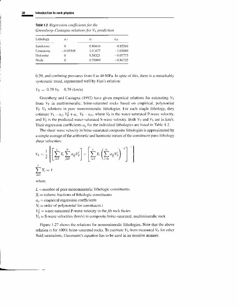
38 Introduction to rock physics-

Tabfe 1,2 Regres.siort cofficients .fbr the

G re e nb e rg-C a s t a I nLt re I ut io ns .fo r V s p re d ic t io n

Li thology l iz l i t ( t ig

Sandstone 0 0.80416 -0.8-5588

Limestone -0.05-508 1.01671 - I .03049

Dolomire 0 0.-58321 -0.01115

Shale 0 0.76969 -0.86735

0.39, and confining pressures from 0 to 40 MPa. ln spite of this, there is a remarkably

systematic trend, represented well by Han's relation:

Vs : 0.19 Vp - 0.19 (km/s)

Greenberg and Castagna (1992) have given empirical relations for estimating V5

from Vp in multimineralic, brine-saturated rocks based on empirical, polynomial

Vp-Vs relations in pure monomineralic l i thologies. For each single l ithology, they

estimate Vs: aiz. Vf, + u;1 Vp I ato, where Vp is the water-saturated P-wave velocity,

and Vs is the predicted water-saturated S-wave velocity. Both Vp and V5 are in km/s.

Their regression coetficients at for the individual l i thologies are l isted in Table 1.2.

The shear-wave velocity in brine-saturated composite lithologies is approximated by

a simple average of the arithmetic and harmonic means of the constituent pure-lithology

shear velocities:

, [ f , N I l - L / N , \ ' l ' lv . : l f l i X , f o ; ; v ' , | * | i x , { i r , ' , v l l I I' r - 1 l l L " t L " ' L

I l - 1 ' - ' t J ' e 1 | f- [ L ; - t i : r J f i - t \ r o / ) |

L

I t ' : t

where

L: number of pure monomineralic l i thologic constituents

Xi : volume fractions of lithologic constituents

at : empirical regression coefficients

Ni : order of polynomial fbr constituent i

Vl : *ater-saturated P-wave velocity in the jth rock facies

Vs : S-wave velocities (km/s) in composite brine-saturated, multimineralic rock

Figure 1.27 shows the relations for monomineralic lithologies. Note that the above

relation is for 1007o brine-saturated rocks. To estimate V5 from measured 7p lbr other

fluid saturations, Gassmann's equation has to be used in an iterative manner.

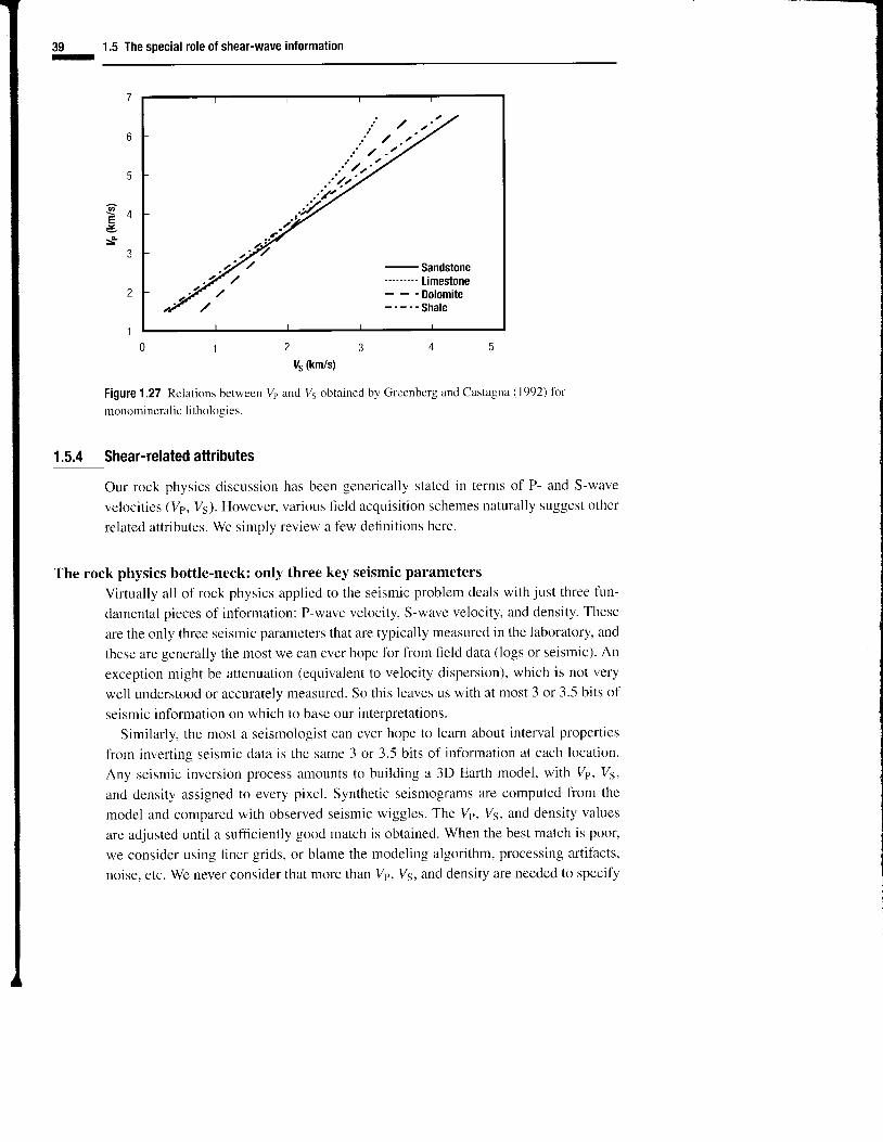
..,i.:/..t1-2

39n

1.5 The special role of shear-wave information

{ A

5s'

3

Figwe 1.27 Relations between

monomineral ic l i thologies.

1.5.4 Shear-relatedattributes

Ys (km/s)

Vp and Vs obtained by Greenberg and Castagna (1992) for

Our rock physics discussion has been generically stated in terms of P- and S-wave

velocities (Vp, Vs). However, various field acquisit ion schemes naturally suggest other

related attributes. We simplv review a f-ew definitions here.

The rock physics bottle-neck: only three key seismic parameters

Virtually all of rock physics applied to the seismic problem deals with just three fun-

damental pieces of intormation: P-wave velocity, S-wave velocity, and density. These

are the only three seismic parameters that are typically measured in the laboratory, and

these are generally the most we can ever hope fbr from field data (logs or seismic). An

exception might be attenuation (equivalent to velocity dispersion), which is not very

well understood or accurately measured. So this leaves us with at most 3 or 3.5 bits of

seismic information on which to base our interpretations.

Similarly, the most a seismologist can ever hope to learn about interval properties

fiom inverting seismic data is the same 3 or 3.5 bits of information at each location.

Any seismic inversion process amounts to building a 3D Earth model, with 7p, Vs,

and density assigned to every pixel. Synthetic seismograms are computed from the

model and compared with observed seismic wiggles. The Vp, V5, and density values

are adjusted until a sufficiently good match is obtained. When the best match is poor,

we consider using finer grids, or blame the modeling algorithm, processing artifacts,

noise, etc. We never consider that more than Vp, V5, and density are needed to specify

/oas .1 /- .,r// ' *l " / :

1^,,"

40 Introduction to rock physicsI

4

3.5

3

3.5

3

c 2.5

5 2g

1 . 5

1

0.5

0

G2.5

5 2g

1 . 5

1

0.5

00 1 2 3 4 5 6 7 8 0 1

t/p (km/s)2 3 4 5 6 7 8

Yp (km/s)

Figure 1,28 Estimating the best-case, error-free rock properties can be useful. On the lefi, soft,high-porosity rocks with good potential fbr detecting pressure and saturation changes. There is a lotof overlap in Vp only, but not in the 2D Vp-Vs plane. On the right, low-porosity stifT rocks ofl'eringlittle chance of detecting fluid and pressure eff-ects - the problem is close to hopeless, suggestingthat special shear acquisition would be a waste.

the rock properties, except for Q or attenuation, or velocity dispersion, or anisotropy.

In fact, the wave equation doesn't require anything more. The main reason that many

more attributes are sometimes measured is to reveal the peontetric arransenTenl of rock

types.

A related discussion is to show how to use calibration data to estimate quantitatively

the rock physics uncertainty when interpreting data. For any given reservoir, we believe

it is useful to quantify the "best-case" interpretation uncertainty that we would have

if we could measure Vp, Vs, and density error-free. In this case, the interpretation

accuracy will be limited by geologic parameters, such as mineralogy, pore stiffness, fluid

contrasts, shaliness, etc. This is the "intrinsic resolvabil ity" ofthe reservoir parameters.

The value of quantifying the best-case uncertainty is that we will be able to identify

and avoid hopeless interpretation problems right from the start. These will be the field

problems where no amount of geophysical investment will allow accurate rock physics

interpretation (Figure 1.28).

For most other situations, we can estimate how the uncertainty worsens compared

with the best case, ( I ) when measurement errors are introduced, (2) when we drop fiom

three parameters to two (e.g. Vp, Vs), or (3) when using alternative pairs of attributes(Ro, G, or pVp, pVs, etc.). We believe that this kind rf analysis can be helpful in the

decision-making process to Jind the most cost-effective use of shear-wave data.

Other shear-related attributes

The attribute pairs in the following short list are all algebraically derivable from Vp,

V5, and density, p or their contrasts.

L _ ,

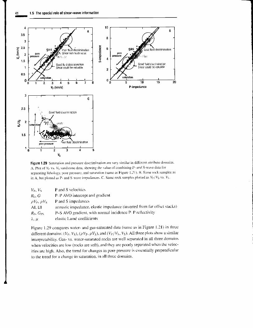
41-

4

0.5

1.5 The special role of shear-wave inlormation

3.5

3

a 2.5

5 2g

1 . 5

1

oo'3 4 5Yp ftm/s)

5 1 0P-impedance

{ 2s"

2.5

1 . 5

Good fluid discrimination

ys

Figure 1.29 Saturation and pressure discrimination are very similar in difl'erent attribute domains.

A. Plot of Vp vs. V5 sandstone data, showing the value of combining P- and S-wave data fbr

separating l ithology, pore pressure, and saturation (same as Figure l.2l). B. Same rock samples as

in A, but plotted as P- and S-wave impedances. C. Same rock samples plotted as Vp/V5 vs. V5.

Vp, Vs P and S velocities

R6, G P-P AVO intercept and gradient

pVp, pVs P and S impedances

AI, EI acoustic impedance, elastic impedance (inverted from far off.set stacks)

Ro, Gps P-S AVO gradient, with normal incidence P-P reflectivity

X, 1r elastic Lam6 coefficients

Figure 1.29 compares water- and gas-saturated data (same as in Figure l.2l) in three

difl-erent domains: (Vp, Vs), (pVp, pV), and(Vplft, ys). All three plots show a similar

interpretability. Gas- vs. water-saturated rocks are well separated in all three domains

when velocities are low (rocks are soft), and they are poorly separated when the veloc-

ities are high. Also, the trend for changes in pore pressure is essentially perpendicular

to the trend fbr a change in saturation, in all three domains.

Good fluid discriminationShear could be valuable

Good fluid discriminationShear could be valuable

42 Introduction to rock physicsI

Information theory tells us that the intrinsic information in a data set does not change

under coordinate transfbrmation. Hence, interpretation of data plotted in the (Vp, Vs)

domain should not be different than, for example, in the (Vp/V5, Vs) domain. On the

other hand, the problem is different in the (p Vp, p 75) domain, because of the additional

parameler . densi ly .

The more important practical consideration, which this theoretical statement ignores,

is the difTerence in measurement effors associated with the different domains. For

example, P-P AVO attributes (Ro, G) have errors associated with noise, amplitude pick-

ing, phase changes with offset, velocity estimation, nonhyperbolic moveout, anisotropy,

fitt ing a sin2 d function to the amplitudes, etc. Values of Vplft determined from com-

paring interval times on P-wave and converted shear-wave stacks have errors associated

with incorect moveout, migration difficulties, anisotropy, time-picking, correlation of

the P and S events, etc. We suspect that image quality, signal-to-noise, and measure-

ment uncertainty, in general, are the biggest practical di1}-erences among the difTerent

types of shear data. A critical part of acquisition decision-making is fbrward modeling

to estimate these erors.

-

1.6 Rock physics "What ifs?": fluid and lithology substitution

One of the most powertul uses of rock physics is extrapolation. At a well - assuming

that data quality is good - we pretty much know "the answer." Cuttings, cores, and logs

tell us about the l ithology, porosity, permeabil ity, and fluids. And, assuming that there

is a good tie between seismic and synthetics, we might even say that we understand the

seismic data at the well.

The problem is, often, knowing what happens as we move away fiom the well. As

we move laterally or vertically, what happens if the porosity changes, or if the l ithology

changes, or if the fluids change? How would the well-log Vp, Vs, and density change?

How would the seismic data change?

This is the role of the rock physics "What fs?" Using the various trends and transfor-

mations presented in this chapter, we can extrapolate to conditions that might exist away

fiom the well, and then compute synthetics to explore how the seismic signatures might

change. This is particularly useful when we wish to understand the seismic signatures

of fluids and facies that are not represented in the well. For statistical methods, such

as clustering analysis or neural networks, such extrapolations are critical fbr extending

the training data.

The best known example is, "What if the pore fluids change?" This is the fluid

substitution problem. In Plate 1.30 we show well logs penetrating a sandy North Sea

turbidite sequence. Along with it (top right) are the corresponding normal-incidence

synthetics, assuming a 50 Hz Ricker wavelet. The initial logs showed an average water

sarurarion of abour 1o7o in the thick sand, with l ight oil of 35 API, GoR (Gas oil

; )eil

1!_ 1.7 All models are wrong. . . some are useful

Ratio) of 200 Sm3/Sm3. we apply a Gassmann ffuid substitution, increasing the watersaturarion to 90Ea, with brine salinity of 30 000 parts per milrion (ppm). The predictedresults are shown ar the bottom of plate I.30. on the lefi, *. ,." that repracing rightoil with water increases the density and p-wave verocity in the sand. The impedanceincreases by about 8o/o'The synthetics show that the fluid substitution results in bothamplitude changes and traveltime pullup (earlier arrivals).A very ditferent rock physics "whai if?,, is whatwe ca1 .. l i thorogy

substitution.,,Plate l '3 I again shows the logs through ttr" ,ondy turbidite sequence as in plate I .30.Now we ask, "what if the porosity .hong.s?" At the top of plate r.3r, we predicra porosity reduction of 370 associated with an increase of cementing. we moder thevelocity change using the cementing trend, described by a modified upper Hashin_Shtrikman bound, as in Figures 1.g and r.t0. we see that decreasing the porosityincreases the clensity in the sand, and causes Isvnrhetics show a rarge change in ampritude ;xTHTn::in

Vp and impedance' The

Atthebot tomofPlate I .3 l ,wepredictaporosi tyreduct ion of3o/o,Lhist imeassociatedwith a deterioration of sorting. we model the velocity change using the sorting trencr,described by a 'ower Hashin-shtrikman bound, as in Figures 1.9 and 1.r0. we seethat decreasing the porosity increases the density in the sand, and causes much sma,erincreases in Vp and impedance.

Fina,y, prate 1.32 shows what happens if the pore pressure changes. In this case,the pore pressure decrines bv s Mpa (effective,;;;#";;;;r,"i'rr"n-' r0 Mpa to,;#;fl.lte

result is virtuallv no errect on densitv, but fairry lorg. i-n.r"ures in zp and

1.7 Alf modefs are wrong . . . some are useful

-

1.7.1

Most rock physics moders relevant to the scope of this book are aimed at describingrelations between measurabre seismic parameters and rock_fluid properties. while it isnot our intention to review ail moders exhaustivery, we find ,rru, -un'y fail within threegeneral classes: theoretical, empirical, and heuristic.

Theoretical models

The theoretical models are primarily continuum mechanics approximations of the elas_tic, viscoerastic, or poroelastic properties of rocks. Among the most famous are theporoelastic moders of Biot (1956), who was among the first to formurate the cou_pled mechanicar behavior of a porous rock embedded with a l inear viscous fluid. TheBiot equations recluce to the f'amous Gassmann (195 l) relations at zerofiequency;hence, we often refer to "Biot-Gassmann,,fluid substitution. Biot (r962) generalized

44 Introduction to rock physicsII

his fbrmulation to include a viscoelastic frame, which was later pursued by Stoll andBryan (1970). The "squirt model" of Mavko and Nur (.19i5) and Mavko and Jizba(199 1) quantif ied a grain-scale fluid interaction, which contributed to the fiame vis-coelasticity. Dvorkin and Nur (1993) explicit ly combined Biot and squirt mechanismsin their "Bisq" model.

Elastic models tend to be ( 1) inclusion models, (2) contact models, (3) computationalmodels, (4) bounds, and (5) transformations.

(1) Inclusion models usually approximate the rock as an elastic solid containingcavities (inclusions), representing the pore space. Because the inclusion cavities aremore compliant than solid mineral, they have the effect of reducing the overall elas-tic stiffhess of the rock in either an isotropic or anisotropic way. The vast majorityof inclusion models assume that the pore cavities are ell ipsoidal or "penny-shaped"(Eshelby, 1957; Walsh, 1965; Kuster and Toksoz, 1974; O'Connell and Budiansky,1974,1977 Cheng, 1978, 1993; Hudson, 1980, 1981, t990; Crampin, t984; Johansenet al., 2002). Berryman ( 1980) generalized the self-consistent description so that boththe pores and grains are considered to be ellipsoidal "inclusions" in the composite.Mavko and Nur (1978) and Mavko (1980) also considered inclusion cavities that werenon-ell ipsoidal in shape. Schoenberg (1983) and Pyrak-Nolte et al. (1990a,b) haveconsidered inclusions in the form of infinite planes of slip or compliance, as models offractures.

Inclusion models have contributed tremendous insights as elastic analogs of rockbehavior. However, their limitation to idealized (and unrealistic) pore geometries hasalways made comparing the models to actual pore microgeometry difficult. For example,relating inclusion models to variations of rock texture resulting from different deposi-tional or diagenetic processes is not feasible. Quite simply, if we observe a rock in thinsection, scanning electron microscope (SEM) image, or outcrop, we really do not havea satisfactory way of choosing model parameters (such as inclusion density and aspectratio) to describe what we see. Workers often "invert" for the model parameters thatgive a good fit to measured elastic properties, but the question always remains, "Howwell do these parameters represent real rock textures?"

(2) Contact models approximate the rock as a collection of separate grains, whoseelastic properties are determined by the deformability and stiffness of their grain-to-grain contacts. Most of these (walton, 1987; Digby, I 981 ; Norris and Johnson , 1991:Makse et al., 1999) are based on the Hertz-Mindlin (Mindlin. 1949) solution for theelastic behavior of two elastic spheres in contact. The key parameters determining thestiffness of the rock are the elastic moduli of the spherical grains and the area of graincontact, which results from the deformability of the grains under pressure. Dvorkinand Nur (1996) described the effect of adding small amounts of mineral cement at thecontacts of spher ica l gra ins.

As with the inclusion models, the spherical contact models have served as usefulelastic analogs of soft sediments, but they also suffer from their extremely idealized

45r

1.7 All models are wrong . . . some are useful

geometries. They are not easy to extend to realistic grain shapes, or distributions of

grain size. Furthermore, the most rigorous part of the contact models is the formal

description of a single grain-to-grain contact. To extrapolate this to a random packing

of spheres makes sweeping assumptions about the number of contacts per grain, and

the distribution of contact fbrces throughout the composite.

(3) Computational models are a fairly recent phenomenon. In these, the actual grain-

pore microgeometry is determined by careful thin-section or CT-scan imaging. This

geometry is represented by a grid, and the elastic, poroelastic, or viscoelastic behavior is

computed by "brute force," using finite-element, finite-difl'erence, or discrete-element

modeling. Clear advantages of these models are the freedom fiom geometric idealiza-

tions, and the ability to elastically quantify features observed in thin section. A second,

older class of computational contact models are the discrete-element models, which

attempt to simulate the simultaneous interactions of many fiee-body grains in a sofi

sediment.(4) Bounds, such as the Voigt-Reuss or Hashin-Shtrikman bounds presented in this

chapter are, in our opinion, the "silent heroes" of rock models. They are extremely

robust and relatively free of idealizations and approximations, other than representing

the rock as an elastic composite. Originally, bounds were treated only as describing

the limits of elastic behavior; some even considered them of only limited usefulness.

However, as shown in Chapters I and2, they have turned out to be valuable "mixing

laws" that allow accurate interpolaticn of sorting and cementing trends, as well as being

the rigorously correct equations to describe suspensions and fluid mixtures.

(5) Transformations include models such as the Gassmann (195 l) relations for

fluid substitution, which are relatively fiee of geometric assumptions. The Gassmann

relations take measured 7p and V5 at one fluid state and predict the Vp and V5 at

another fluid state. Beryman and Milton (1991) presented a geometry-independent

scheme to predict fluid substitution in a composite of two porous media having separate

mineral and dry-frame moduli. Mavko et al. (1995) derived a geometry-independent

transformation to take hydrostatic velocity vs. pressure data and predict stress-induced

anisotropy. Mavko and Jizba ( I 99 I ) presented a transformation of measured dry velocity

vs. pressure to predict velocity vs. frequency in fluid-saturated rocks.

1.7.2 Empiricalmodels

Empirical models do not require much explanation. The approach is generally to assume

some function form and then determine coefficients by calibrating a regression to

data. Some of the best known are Han's ( 1986) regressions for velocity-porosity-clay

behavior in sandstones, the Greenberg-Castagna (1992') relations for Vp-V5, and the

Vp-density relations of Gardner et al. (1914). A particularly popular form of empirical

approach is to use neural networks as a way to determine nonlinear relations among

the various parameters.

46 Introduction to rock physics-

Empirical relations are sometimes disguised as theoretical. For example, the popularmodel of Xu and White ( 1995) for Vs prediction in shaly sands is based on the Kuster-Toksciz ell ipsoidal inclusion formulation. One unknown aspect ratio is assigned torepresent the compliant clay pore space, and a second unknown aspect ratio is assignedto represent the stiff'er sand pore space. These aspect ratios are determined empiricallyby calibrating to training data. In other words, this is an empirical model, in which thefunction form of the regression is taken fiom an elastic model.

It is useful to remember that all empirical relations involve this two-step processof a modeling step to determine the functional fbrm fbllowed by a calibration stepto determine the empirical coefficients. We sometimes forget that the common linearregression involves a very deliberate modeling step of deciding that there is a l inearrelation between the two variables.

1.7.3 Heuristic models

Heuristic models are what we might call "pseudo-theoretical." A heuristic model usesintuit ive, though nonrigorous, means to argue why various parameters should be relatedin a certain way.

The beslknown heuristic rock physics model is the Wyllie time average, relatingveloc i ty toporosi ty , l lV:SlVn, , ia*( l - Q) lV^ in,ur . At f 'acevalue, i t looksl iketheremight be some physics involved. However, the time-average equation is equivalent to astraight-ray, zero-wavelength approximation, neither of which makes any sense whenmodeling wavelengths that are very long relative to grains and pores. We find thatthe Wyllie equation is sometimes a useful heuristic description of clean, consolidated,water-saturated rocks, but certainly not a theoretically justifiable one.

Other very useful heuristic models are the use of the Hashin-shtrikman upper andlower bounds to describe cementing and sorting trends, as discussed in Chapters Iand 2. Certainly the Hashin-Shtrikman curves are rigorous bounds, for mixtures ofdifTerent phases. However, as we wil l discuss in Chapter 2, we often use the bounds asinterpolatnrs to connect the mineral moduli atzero porosity, with moduli of well-sortedend members at critical porosity. We give heuristic arguments justifying why an upperbound equation might be expected to describe cementing, which is the stiffest way toadd mineral to a sand, and why a lower bound equation might be expected to describesorting. But we are not able to derive these from first principles.

1.7.4 Our hybrid approach

We have had considerable rock physics success using a hybrid of theoretical, empir-ical, and heuristic models to describe clastic sediments. In this sense. we find our-selves thinking more as engineers than physicists - what Amos Nur l ikes to call "dirty

science."

47I

1.7 All models are wrong . . . some are useful

It started with Han's empirical discovery (Chapter l) that velocity-porosity in shaly

sands could be well described by a set of parallel contours of constant clay. Amos Nur

noted that each ofthese contours had high- and low-porosity intercepts that had a clear

physical interpretation: in the limit of zero porosity, any model should rigorously take on

the properties of pure mineral, while in the limit of high porosity (the critical porosity),

the rock should lall apart. When a rock is falling apart, it becomes a suspension, which

is rigorously modeled with a lower bound equation. Eventually Han's contours were

replaced by modified upper bound.r (Chapters I and 2), partly because they fit the data

better over a large range ofporosities, and partly because we could heuristically defend

them. We came to understand that these modified upper bounds described the diagenetic

or cementation trend for sedimentary rocks.

We eventually fbund thatamodified loyver bound (Chapters I and2) was an excellent

description <>f the sorting, trend in velocity-porosity. Again, this was more of an empiri-

cal observation, aesthetically symmetric to the modified upperbound, but not rigorously

def'endable. Jack Dvorkin introduced the friable sand model (Chapter 2), which uses a

theoretical elastic contact model to describe clean, well-sorted sands, combined with a

modified lower bound to interpolate these to lower porosity, poorly sorted sands.

In summary, the rock physics modeling approach presented throughout this book

is the one that we have fbund works well. We avoid over-modeling with too much

theory, fiankly, because we have lost patience with model parameters that fbllow from

assuming spheres and ellipsoids, rather than from geologic processes. We have also

found it dangerous to become attached to meticulously derived theoretical models,

which can never approach the complexity of nature. At the same time, we like to honor

physical principles, because they make the models universal. As time goes on, it almost

seerns that we throw away more and more equations, and replace them with clever use

of various bounds. Another important driver in our approach is our desire to discover,

understand, and quantifv the elastic properties of geologic prutcesses.

We hope that the following chapters will not only illustrate this modeling approach,

but also iustitv it.