1. INTRODUCTION · to 250 µg/m . The algorithm implemented in R to determine the number of knots that yields the most precise fit follows Spiriti et al. (2013). The arrows in the

RTI International is a registered trademark and a trade name of Research Triangle Institute.

TO: Amanda CurryBrown and Neal Fann (OAQPS, EPA)

FROM: Breda Munoz and Paramita Sinha

DATE: July 1, 2015

SUBJECT: Parameterizing the Integrated Exposure Response (IER) Function for application in the Benefits Calculator

1. INTRODUCTION Estimating the global burden of disease attributable to ambient fine particle (PM2.5) exposure requires estimates of the shape and magnitude of the relative risk (RR) function. However, there is limited information on the RR function at different high concentrations in many regions across the world. Burnett et al. (2014) developed RR functions over the entire global exposure range for causes of mortality including ischemic heart disease (IHD), cerebrovascular disease (CEV), chronic obstructive pulmonary disease (COPD) and lung cancer (LC), as well as the incidence of acute lower respiratory infection (ALRI). An Integrated Exposure Response (IER) function was estimated by fitting available information on RR functions from existing studies.1.

This memo summarizes the results of RTI’s efforts to parameterize the IER function so that it can be incorporated in different tools that are used to quantify and value changes in air pollution-related deaths and illnesses such as BenMAP-CE and the Benefits Calculator. A degree-1 spline was proposed by the U.S. Environmental Protection Agency (EPA) as being the most suitable functional form for incorporating in BenMAP. Preliminary exploratory work conducted by EPA fit a 5-knot degree-1 spline for IHD, CEV, COPD, and LC. RTI’s task was to explore whether this fit could be improved by incorporating a different number of knots while considering that the results will be applied in various benefits tools. As per guidance from EPA, the IER function needs to be parameterized for a PM range of 1 µg/m3 to 250 µg/m3 and 1 µg/m3 to 1,000 µg/m3.The following steps2 were taken to accomplish this task:

1. RTI explored whether fitting a degree-1 spline (rather than higher degrees) would result in large losses in accuracy to ensure that using linear splines in BenMAP would not provide inaccurate estimates. This is summarized in Section 2.

2. A large number of knots is likely to pose computational issues in BenMAP, but a small number may result in less accuracy. To balance accuracy and computational

1 Studies on ambient air pollution (AAP), secondhand tobacco smoke (SHS), household solid cooking fuel (HAP) and active smoking (AS) were used. 2 Appendix A summarizes the programming steps and R functions that were used.

Amanda CurryBrown and Neal Fann July 1, 2015 Page 2

convenience, RTI determined the optimal number of knots for each of the four health end points. The decision on the number of knots was based on EPA’s guidance that an acceptable margin of error between RR calculated using the IER and the spline approach would be 1% for the purpose of our task. Using this guidance, we defined a criteria for selecting the optimal number of knots. This is summarized in Section 3.

3. RTI fit splines with the optimal number of knots. A comparison of the results with the optimal number of knots for each end point and a 5-knot spline for all four end points was completed for both PM ranges. This is summarized in Section 4.

4. After EPA review of our results from steps 1 through 3, RTI will produce a BenMAP-ready file. The next steps are summarized in Section 5.

2. LINEAR VERSUS NON-LINEAR SPLINES EPA provided several R scripts and a csv file for calculating the RR distribution of observing each end point at particulate matter (PM) levels ranging from 1 µg/m3 to 250 µg/m3 (integer values only). The csv file, IER Parameter Estimates.csv, contains 1,000 values for the following parameters: alpha, beta, delta, and the cutoff zcf for each end point. For example the first three rows for IHD are listed below:

alpha - IHD beta - IHD delta - IHD zcf - IHD

1.411652 0.062647 0.412676 6.463049

1.217816 0.028152 0.786667 6.533716

1.203071 0.058444 0.522358 7.087289

The script R code to plot IER model with Cis.R was used to calculate the RR and lower and upper 95% confidence intervals for the RR for PM values ranging from1 µg/m3 to 250 µg/m3 (integer values) for each end point. The RR values for end point X (where X = IHD, CEV, COPD, and LC) were calculated using the following mathematical equation:

𝑅𝑅𝑅𝑅 = �1 𝑖𝑖𝑖𝑖 𝑃𝑃𝑃𝑃 < 𝑧𝑧𝑐𝑐𝑐𝑐

1 + 𝛼𝛼 ∗ 𝑋𝑋 ∗ �1 − 𝑒𝑒−𝛽𝛽𝛽𝛽∗�𝑃𝑃𝑃𝑃−𝑧𝑧𝑐𝑐𝑐𝑐�𝛿𝛿� 𝑖𝑖𝑖𝑖 𝑃𝑃𝑃𝑃 ≥ 𝑧𝑧𝑐𝑐𝑐𝑐

These RR values were used to identify the number of knots needed to achieve 1% of precision as suggested by EPA.

To determine the number of knots for fitting a spline, the function fit.search.numknots from the R-library freeknotsplines was modifed to output the statistic modified-GCV (modified


generalied cross-validation criterion). The GCV statistic can be used to determine the number of knots that yields the most precise fit, that is, when GCV is minimized. The GCV is a function of the residual sum of squares (RSS); therefore the number of knots with the most precise fit also renders a spline with minimal RSS (Spiriti et al., 2013). A function findnots() was created to output the GCV, for a combination of spline degrees and range of knots (see Appendix A).

When fitting splines to a set of data, the usual recommendation is to have at least five observations for each parameter to get a stable solution (Wold, 1974; Smith, 1979). A spline of degree p with q knots has p+q parameters, therefore the minimum number of observations needed for a stable solution should be 5 × (p + q). Increasing the number of knots allows the spline to closely follow the data. Increasing the degree also results in a smoother graph, but to a lesser extent. Specifying a large number of knots is better than increasing the degree beyond three (Wold, 1974). This fitting paradigm is implemented in the R-function used to estimate the appropriate number of knots.

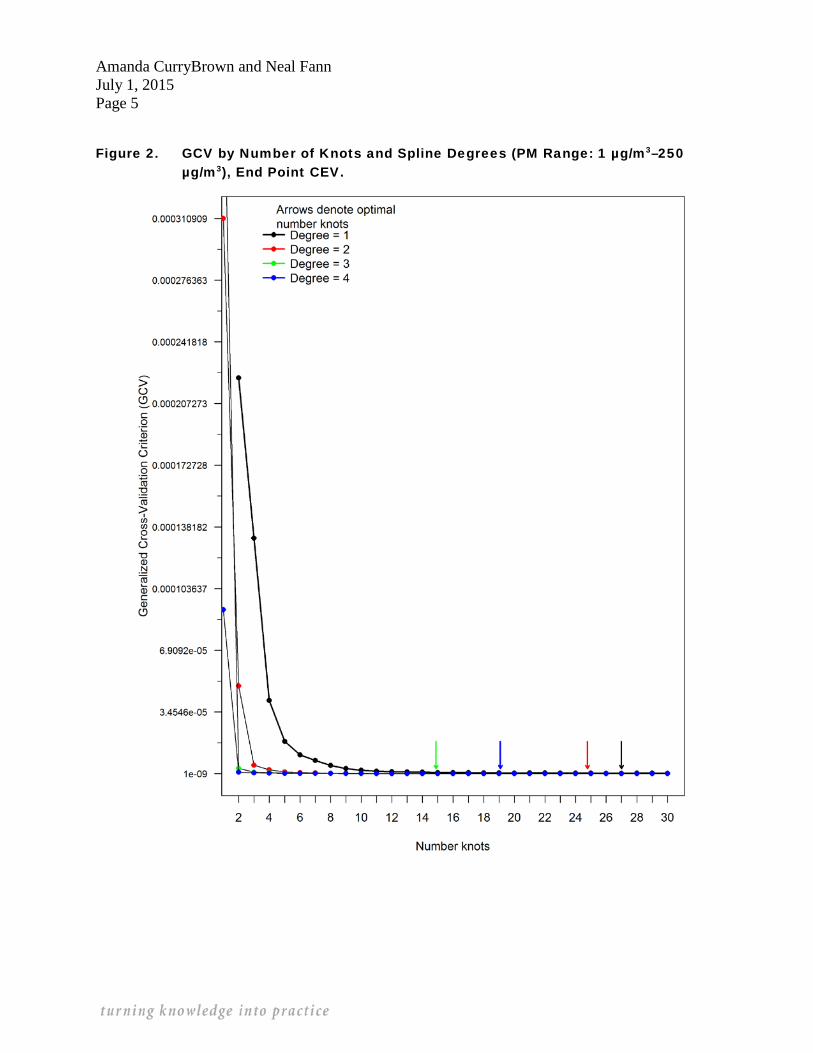
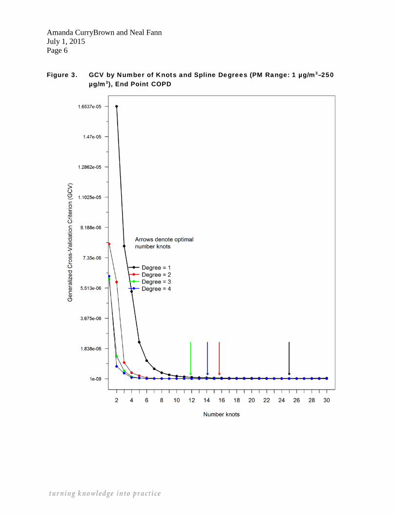
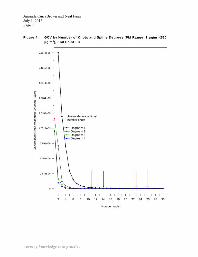
Figure 1 displays the GCV for splines with degrees from 1 to 4 fitted to IER output for IHD for PM range 1 µg/m3 to 250 µg/m3. The algorithm implemented in R to determine the number of knots that yields the most precise fit follows Spiriti et al. (2013). The arrows in the plot denote the number of knots that yields the most precise fit for a specified degree. For example, the number of knots that yields the most precise fit for a spline with degree 1 is 25, and for a spline with degree 2 is 14. For each degree, the change in GCV is negligible when the number of knots is 9 or larger. When the number of knots is 5 or more, the GCV is less than 1.0354e-05 for all splines considered (degrees 1 to 4). Based on these results, it was decided to investigate the precision achieved when using 1-degree splines and number of knots not exceeding 25 for the PM range of 250 µg/m3, and no more than 40 knots for PM range of 1,000 µg/m3. Figures 2 through 4 display a similar relatonship between spline degrees and knots for end points CEV, COPD and LC.


Figure 1. GCV by Number of Knots and Spline Degrees (PM Range: 1 µg/m3–250 µg/m3), End Point IHD


Figure 2. GCV by Number of Knots and Spline Degrees (PM Range: 1 µg/m3–250 µg/m3), End Point CEV.


Figure 3. GCV by Number of Knots and Spline Degrees (PM Range: 1 µg/m3–250 µg/m3), End Point COPD


Figure 4. GCV by Number of Knots and Spline Degrees (PM Range: 1 µg/m3–250 µg/m3), End Point LC


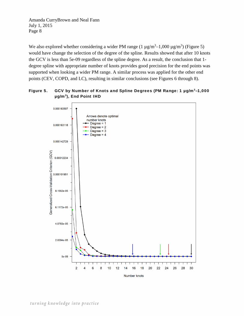
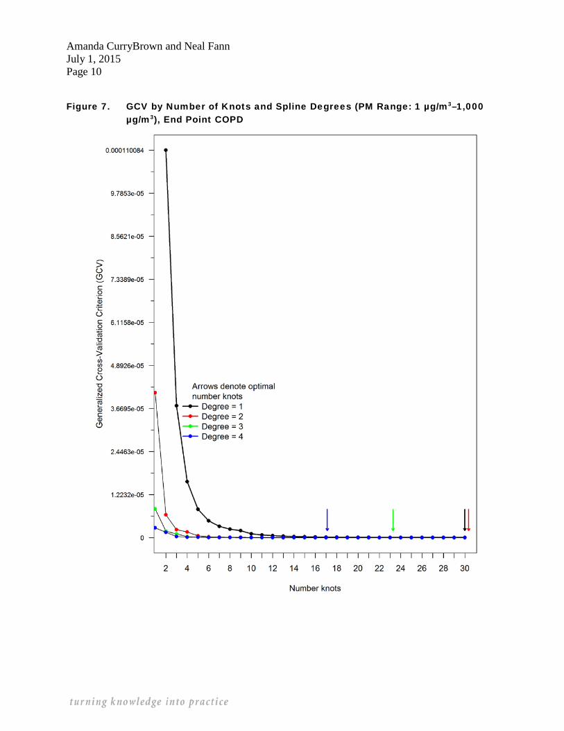
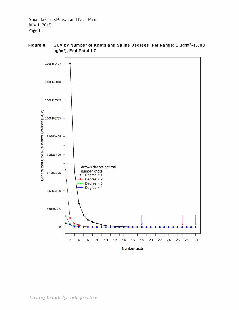
We also explored whether considering a wider PM range (1 µg/m3–1,000 µg/m3) (Figure 5) would have change the selection of the degree of the spline. Results showed that after 10 knots the GCV is less than 5e-09 regardless of the spline degree. As a result, the conclusion that 1-degree spline with appropriate number of knots provides good precision for the end points was supported when looking a wider PM range. A similar process was applied for the other end points (CEV, COPD, and LC), resulting in similar conclusions (see Figures 6 through 8).

Figure 5. GCV by Number of Knots and Spline Degrees (PM Range: 1 µg/m3–1,000 µg/m3), End Point IHD


Figure 6. GCV by Number of Knots and Spline Degrees (PM Range: 1 µg/m3–1,000 µg/m3), End Point CEV


Figure 7. GCV by Number of Knots and Spline Degrees (PM Range: 1 µg/m3–1,000 µg/m3), End Point COPD


Figure 8. GCV by Number of Knots and Spline Degrees (PM Range: 1 µg/m3–1,000 µg/m3), End Point LC


Summary: ■ For all endpoints and splines with degrees 1 to 4 and PM range from 1 µg/m3 to 250

µg/m3, the GCV for 5 or more knots is less or equal than 1.727e-05. The same conclusion remains when the PM range is 1 µg/m3 to 1,000 µg/m3.

■ Regardless of the PM range (1 µg/m3–250 µg/m3 or 1 µg/m3–1,000 µg/m3), when the number of knots is 10 or more, increasing the degree of the spline will not result in significant reductions in GCV. Thus, using a degree-1 spline will not result in large losses in accuracy as compared to larger degree splines, and will comply with EPA’s desired precision (1%).

3. DETERMINING OPTIMAL NUMBER OF KNOTS FOR SPLINE FITTING

We investigated the precision of degree-1 splines with different number of knots for IHD, CEV, COPD and LC for both PM ranges. The most precise 1-degree spline would be obtained by determining the optimal number of knots that minimizes the GCV value (as described in the previous section). However, this would greatly increase the number of knots, especially for the larger PM range of 1 µg/m3 to 1,000 µg/m3 and this may make it computationally prohibitive to include these results in BenMAP. To balance between computational issues in BenMAP and desired accuracy, we define a criteria for determining an optimal number of knots that will serve our purpose. This criteria (described in the following paragraph) is based on EPA’s guidance that an acceptable margin of error between RR calculated using the IER and the spline approach would be 1%.

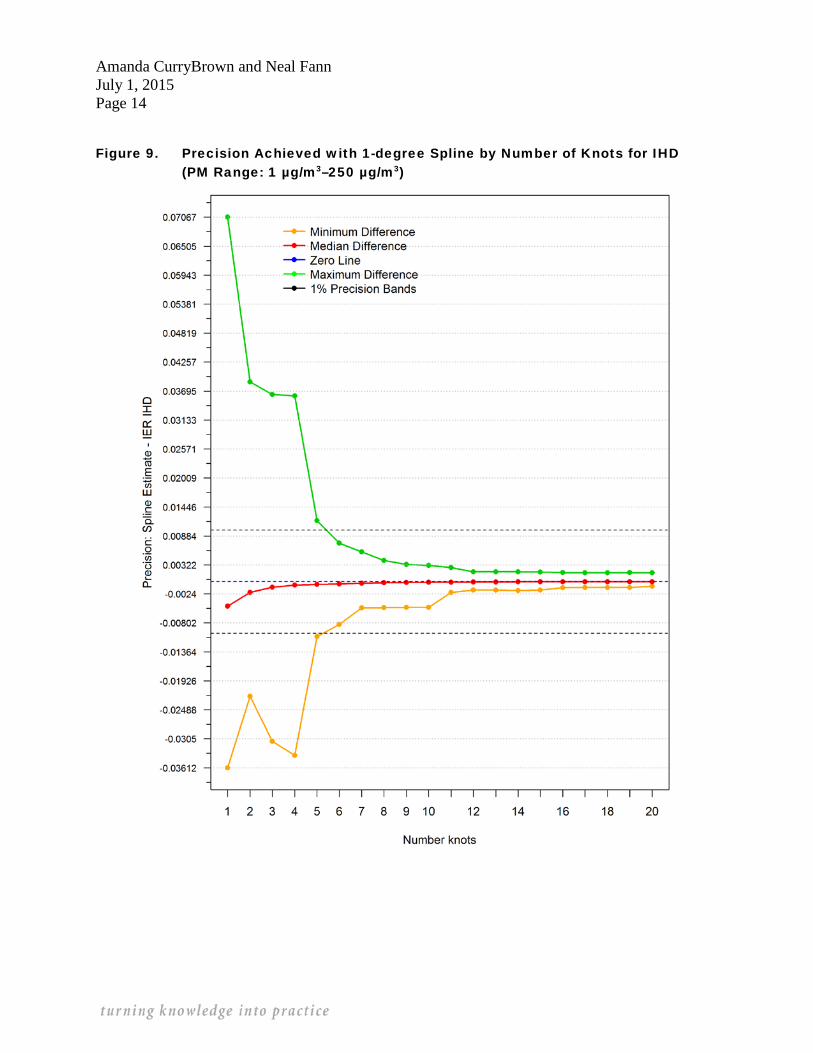
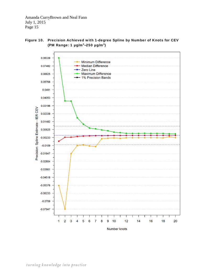
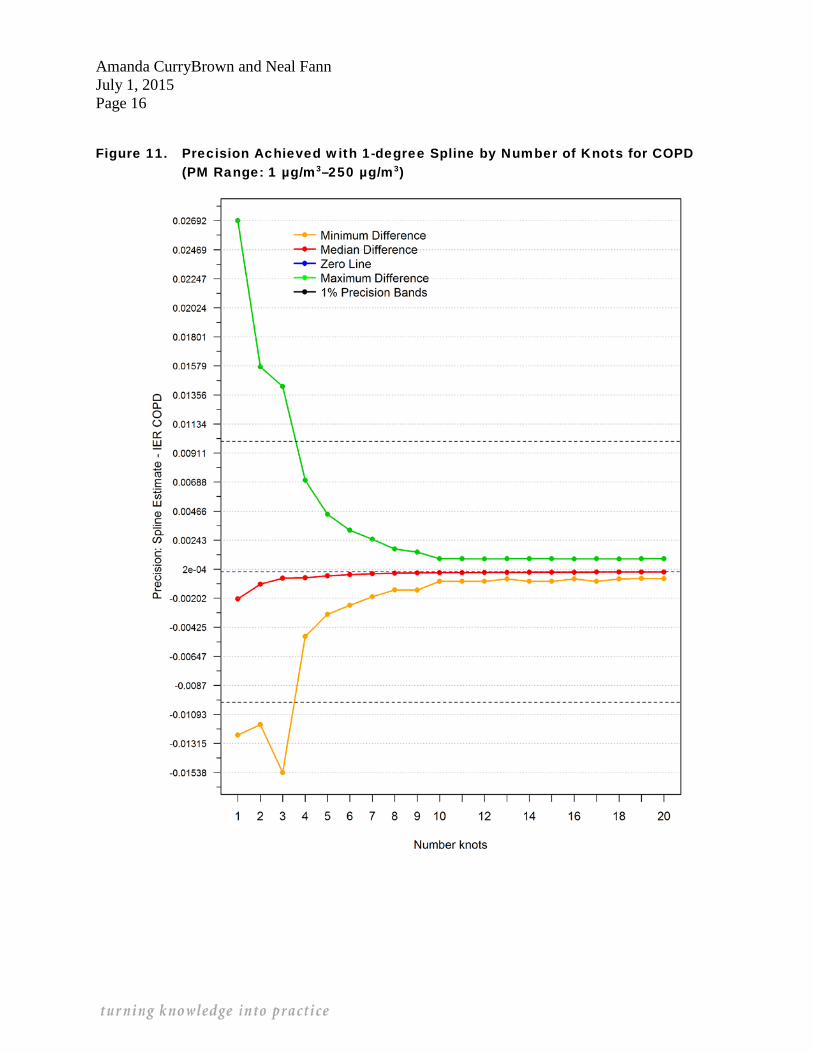
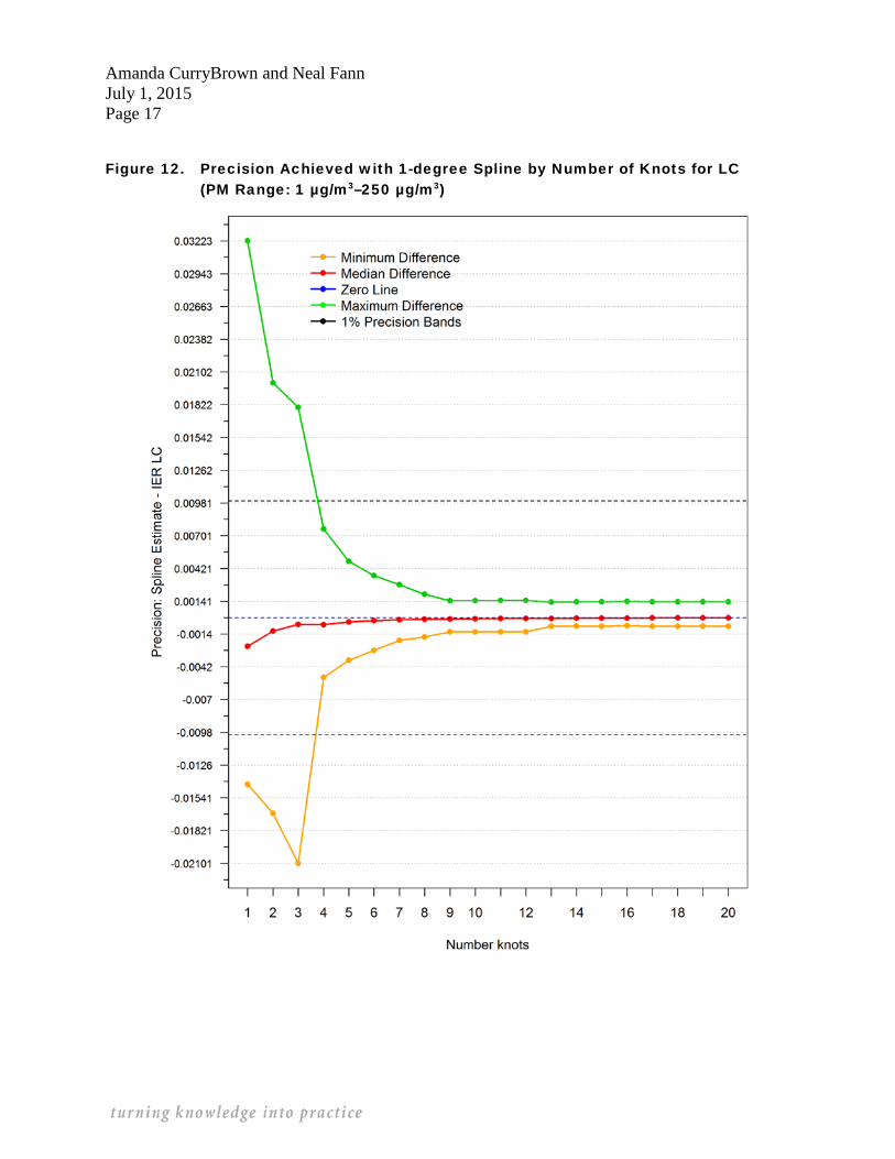
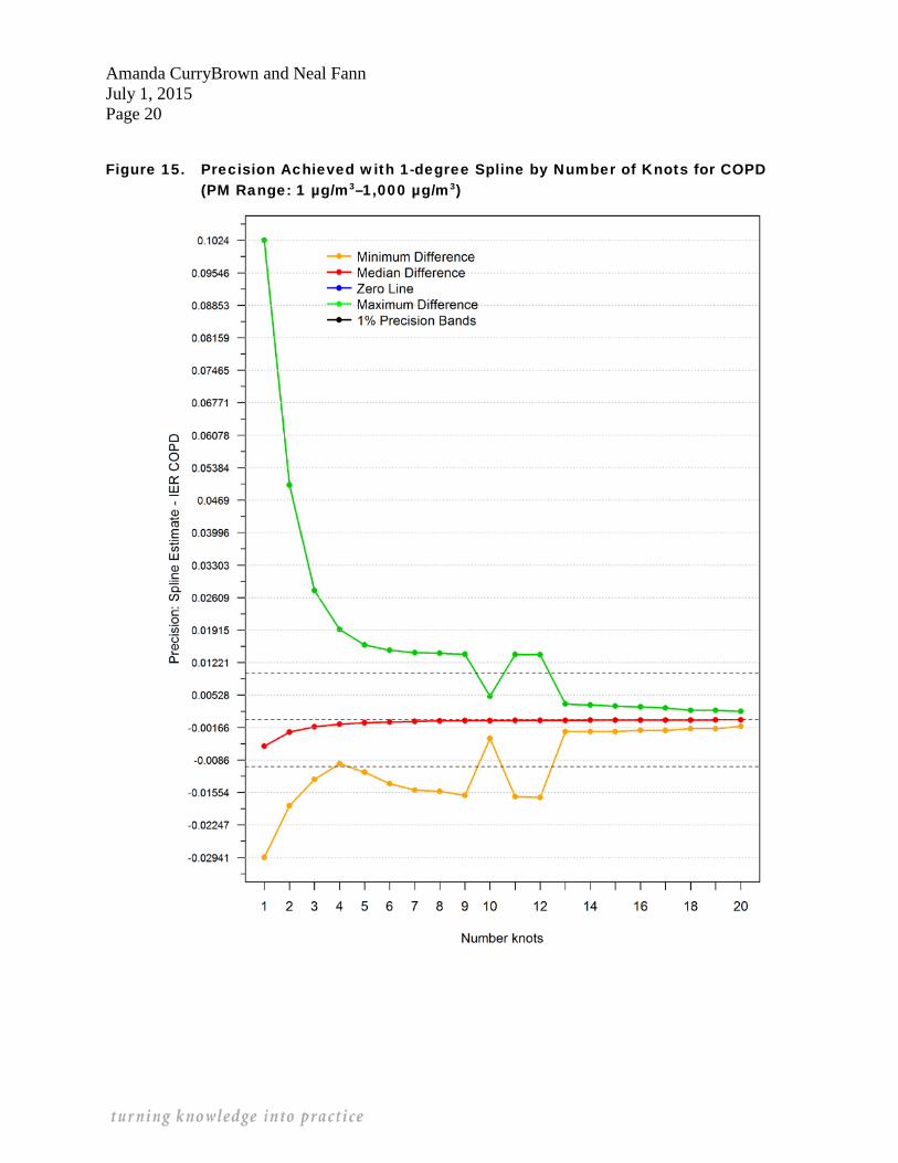
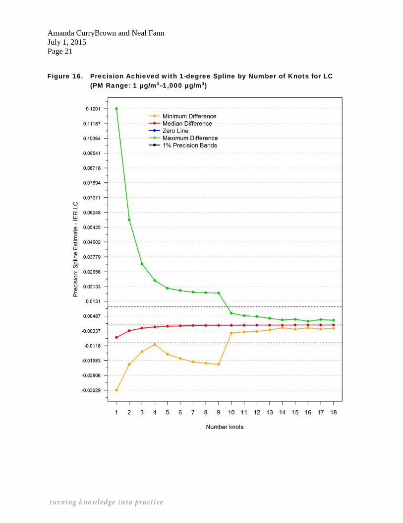
We calculated the deviations between RR calculated using the IER and the corresponding predicted values obtained with 1-degree splines and different number of knots. Negative values of deviations correspond to understimation by the spline and positive values denote overestimation by the spline. We define the optimal number of knots to be the minimum number of knots after which the maximum, minimum, and median deviations are consistently less than 1%.3 The process of selecting the optimal number of knots is illustrated in Figures 9 through 12 3 Note that in previous efforts that involved fitting the spline for a PM range of 1 to 250, we were using our expertise and

judgement to determine the optimal number of knots rather than defining and applying an objective criteria. The number of knots we used certainly met the 1% precision level that EPA desired – in fact, the results were much more precise than the desired 1%. However, the number of knots selected for a PM range of 1 to 250 was larger than was strictly necessary by the 1% criteria. In the current phase of this work, we were tasked with expanding the range of PM to 1000. The previous version of the memo (Munoz and Sinha, 2015) summarized the results for IHD with the expanded PM range. As demonstrated in Table 1 of Munoz and Sinha, 2015, expanding the PM range to 1000 increased the optimal number of knots from 12 to 20 for IHD. Considering the computational issues in BenMAP, we thus defined the new criteria so that it meets EPA’s needs. The new criteria, being completely objective, also has the advantage of being easily replicable and communicable rather than a subjective criteria based on expert judgement. Note also, that should EPA decide to tighten the precision level in the future (for example, if the computational power of BenMAP increases), it will be easy to determine a new set of knots based on the new precision level.


and 13 through 16 for PMs ranging up to 250 µg/m3 and 1,000 µg/m3, respectively. As shown in the figures, the maximum, minimum, and median deviations decrease as the number of knots increase. For the IHD end point (and PM ranging to 250 µg/m3), all three lines cross the 1% band, when the number of knots is 6. Therefore, according to our defined criteria, 6 is the optimal number of knots.


Figure 9. Precision Achieved with 1-degree Spline by Number of Knots for IHD (PM Range: 1 µg/m3–250 µg/m3)


Figure 10. Precision Achieved with 1-degree Spline by Number of Knots for CEV (PM Range: 1 µg/m3–250 µg/m3)


Figure 11. Precision Achieved with 1-degree Spline by Number of Knots for COPD (PM Range: 1 µg/m3–250 µg/m3)


Figure 12. Precision Achieved with 1-degree Spline by Number of Knots for LC (PM Range: 1 µg/m3–250 µg/m3)


Figure 13. Precision Achieved with 1-degree Spline by Number of Knots for IHD (PM Range: 1 µg/m3–1,000 µg/m3)


Figure 14. Precision Achieved with 1-degree Spline by Number of Knots for CEV (PM Range: 1 µg/m3–1,000 µg/m3)


Figure 15. Precision Achieved with 1-degree Spline by Number of Knots for COPD (PM Range: 1 µg/m3–1,000 µg/m3)


Figure 16. Precision Achieved with 1-degree Spline by Number of Knots for LC (PM Range: 1 µg/m3–1,000 µg/m3)


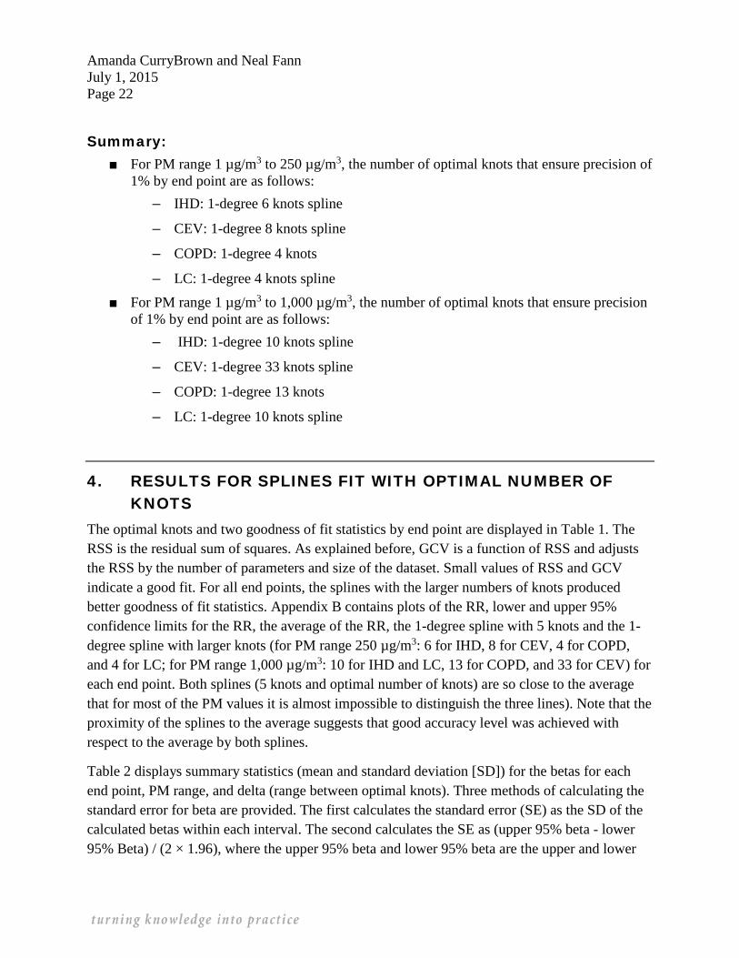
Summary: ■ For PM range 1 µg/m3 to 250 µg/m3, the number of optimal knots that ensure precision of

1% by end point are as follows: – IHD: 1-degree 6 knots spline

– CEV: 1-degree 8 knots spline

– COPD: 1-degree 4 knots

– LC: 1-degree 4 knots spline ■ For PM range 1 µg/m3 to 1,000 µg/m3, the number of optimal knots that ensure precision

of 1% by end point are as follows: – IHD: 1-degree 10 knots spline

– CEV: 1-degree 33 knots spline

– COPD: 1-degree 13 knots

– LC: 1-degree 10 knots spline

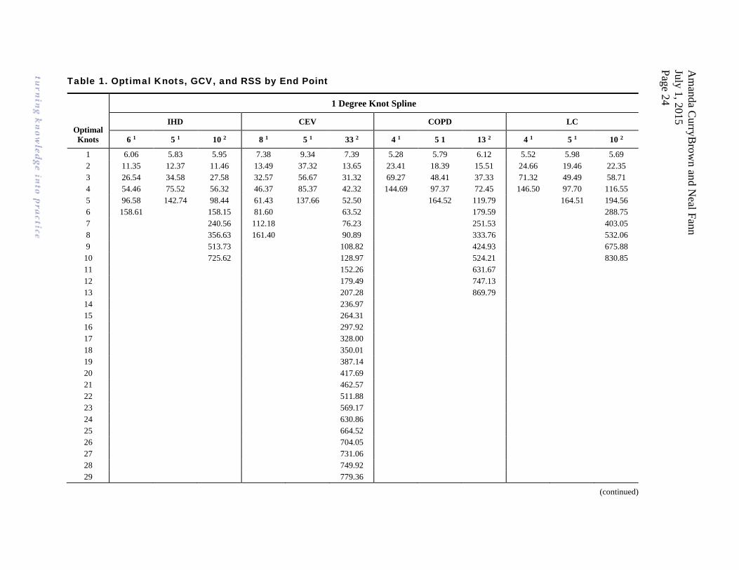
4. RESULTS FOR SPLINES FIT WITH OPTIMAL NUMBER OF KNOTS

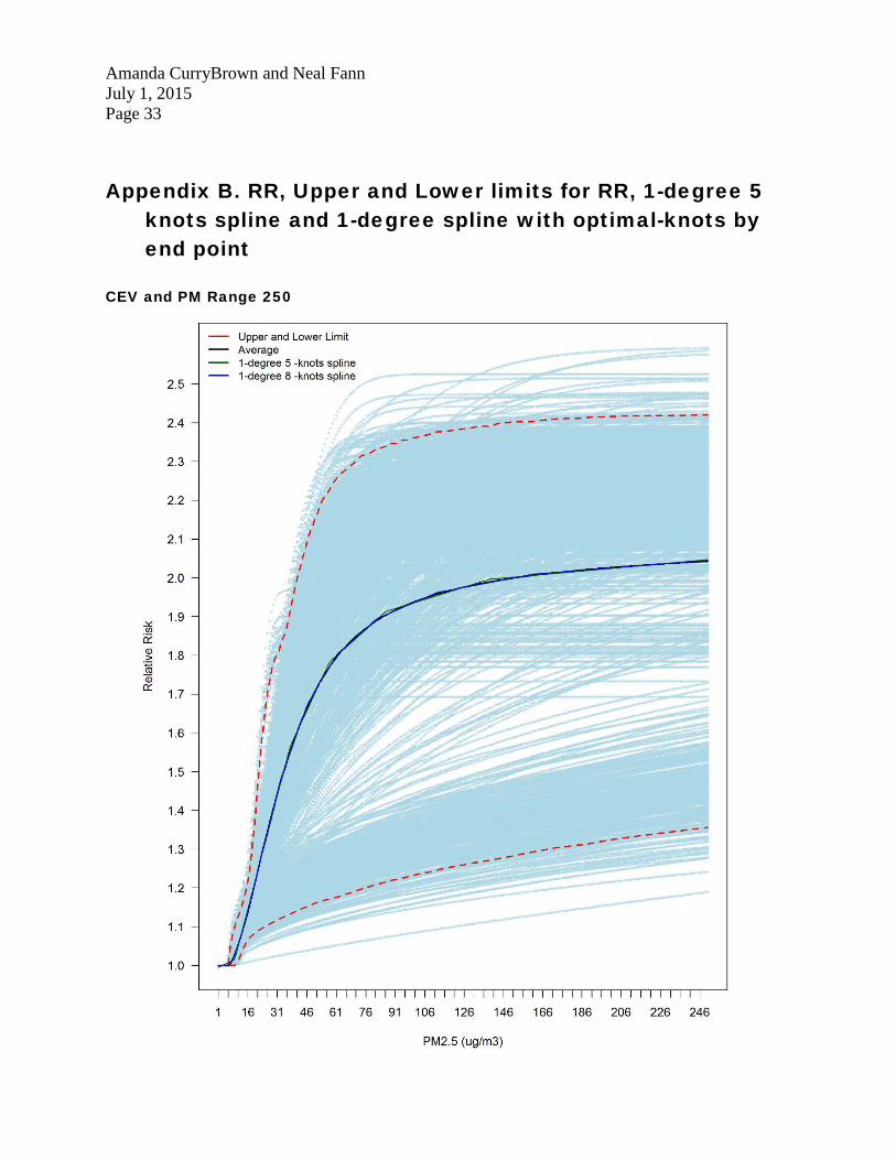
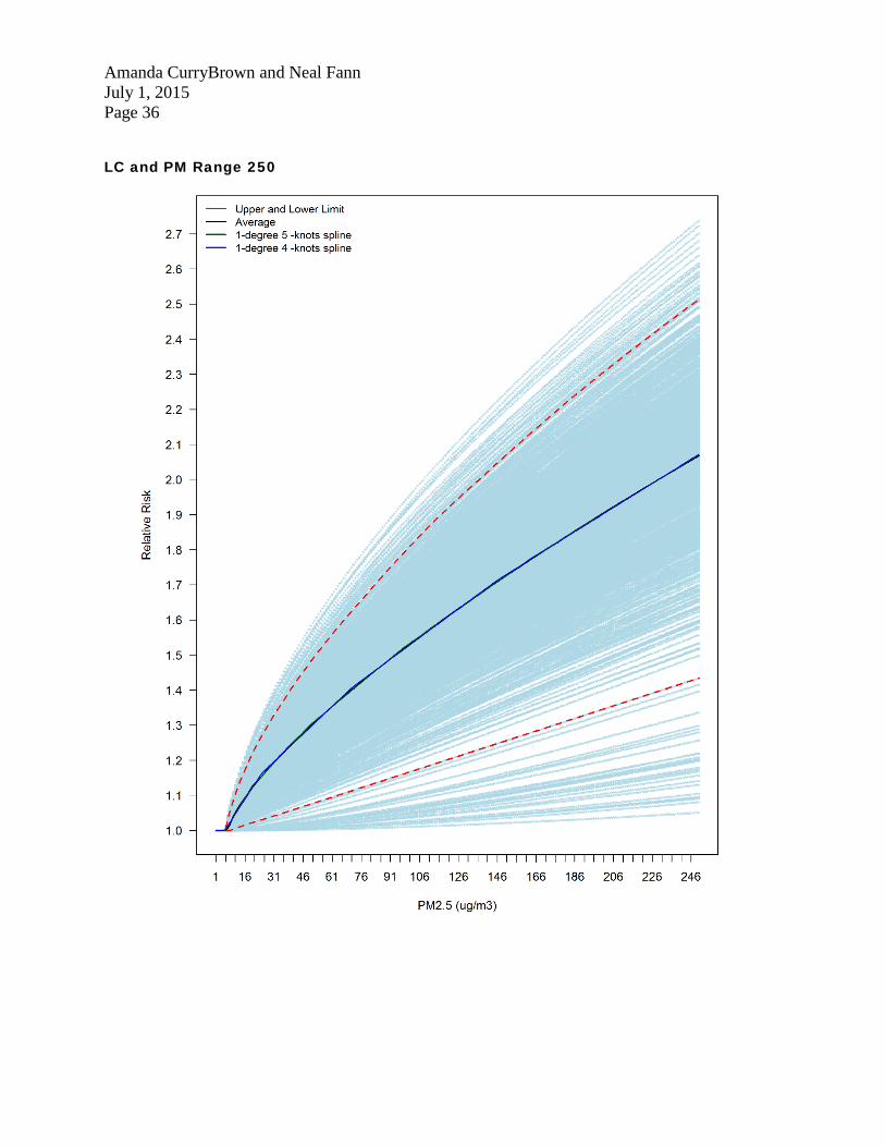
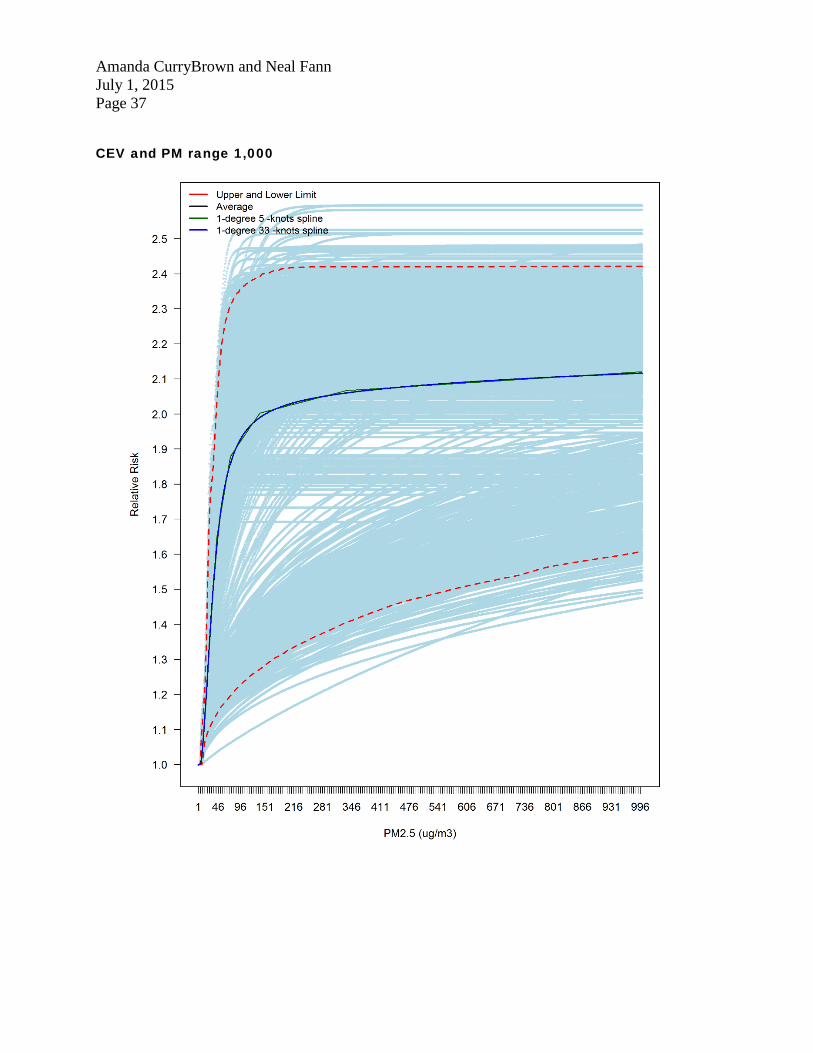
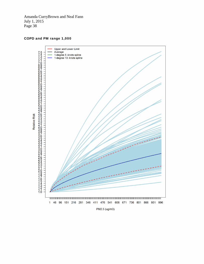
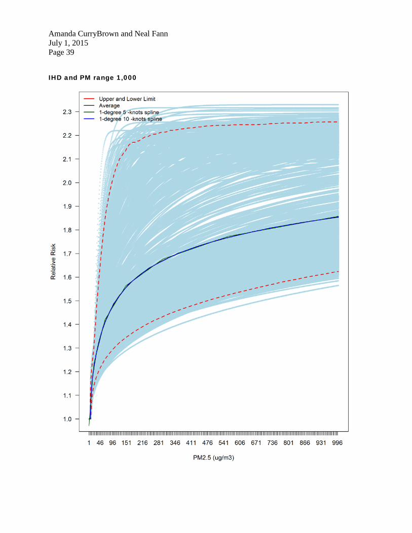
The optimal knots and two goodness of fit statistics by end point are displayed in Table 1. The RSS is the residual sum of squares. As explained before, GCV is a function of RSS and adjusts the RSS by the number of parameters and size of the dataset. Small values of RSS and GCV indicate a good fit. For all end points, the splines with the larger numbers of knots produced better goodness of fit statistics. Appendix B contains plots of the RR, lower and upper 95% confidence limits for the RR, the average of the RR, the 1-degree spline with 5 knots and the 1-degree spline with larger knots (for PM range 250 µg/m3: 6 for IHD, 8 for CEV, 4 for COPD, and 4 for LC; for PM range 1,000 µg/m3: 10 for IHD and LC, 13 for COPD, and 33 for CEV) for each end point. Both splines (5 knots and optimal number of knots) are so close to the average that for most of the PM values it is almost impossible to distinguish the three lines). Note that the proximity of the splines to the average suggests that good accuracy level was achieved with respect to the average by both splines.

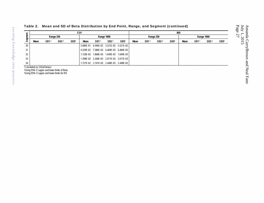
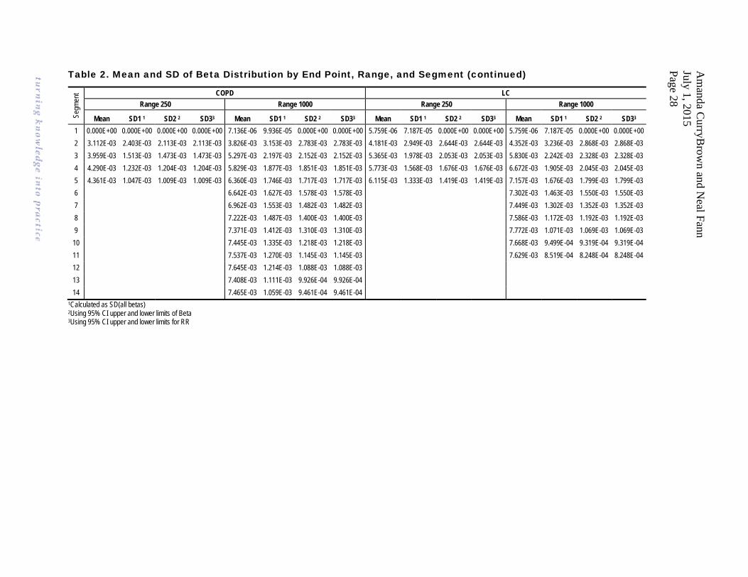
Table 2 displays summary statistics (mean and standard deviation [SD]) for the betas for each end point, PM range, and delta (range between optimal knots). Three methods of calculating the standard error for beta are provided. The first calculates the standard error (SE) as the SD of the calculated betas within each interval. The second calculates the SE as (upper 95% beta - lower 95% Beta) / (2 × 1.96), where the upper 95% beta and lower 95% beta are the upper and lower


limits of a 95% simulation confidence interval for beta within each interval. The 95% confidence interval upper limit is the 97.5 percentile of the beta distribution within that interval; similarly the 95% confidence interval lower limit is the 2.5 percentile of the beta distribution within that interval. The third method is very similar to the second, and it is based on the upper and lower percentiles of the relative risk within each interval.

For some end points and range, the number of beta estimates that are not zero in the first segment is very small. As a result, both the 2.5 and 97.5 percentiles are equal to zero, which translates to a zero SD using method two. Similar reasoning results in zero values for the SD when using method three.

Am

anda CurryB

rown and N

eal Fann July 1, 2015 Page 24

Table 1. Optimal Knots, GCV, and RSS by End Point

Optimal Knots

1 Degree Knot Spline

IHD CEV COPD LC

6 1 5 1 10 2 8 1 5 1 33 2 4 1 5 1 13 2 4 1 5 1 10 2

1 6.06 5.83 5.95 7.38 9.34 7.39 5.28 5.79 6.12 5.52 5.98 5.69 2 11.35 12.37 11.46 13.49 37.32 13.65 23.41 18.39 15.51 24.66 19.46 22.35 3 26.54 34.58 27.58 32.57 56.67 31.32 69.27 48.41 37.33 71.32 49.49 58.71 4 54.46 75.52 56.32 46.37 85.37 42.32 144.69 97.37 72.45 146.50 97.70 116.55 5 96.58 142.74 98.44 61.43 137.66 52.50 164.52 119.79 164.51 194.56 6 158.61 158.15 81.60 63.52 179.59 288.75 7 240.56 112.18 76.23 251.53 403.05 8 356.63 161.40 90.89 333.76 532.06 9 513.73 108.82 424.93 675.88 10 725.62 128.97 524.21 830.85 11 152.26 631.67 12 179.49 747.13 13 207.28 869.79 14 236.97 15 264.31 16 297.92 17 328.00 18 350.01 19 387.14 20 417.69 21 462.57 22 511.88 23 569.17 24 630.86 25 664.52 26 704.05 27 731.06 28 749.92 29 779.36

(continued)

Am

anda CurryB

rown and N


Table 1. Optimal Knots, GCV, and RSS by End Point (continued)

Optimal Knots

1 Degree Knot Spline

IHD CEV COPD LC

6 1 5 1 10 2 8 1 5 1 33 2 4 1 51 13 2 4 1 5 1 10 2

30 808.96 31 866.09 32 895.56 33 947.27

GCV 1.13E-05 9.97E-06 1.53E-06 4.48E-06 1.59E-05 2.46E-09 5.30E-06 1.97E-06 3.98E-07 7.29E-06 2.71E-06 1.61E-06 RSS 1.15E-05 2.35E-03 1.56E-06 4.56E-06 3.76E-03 2.63E-09 5.35E-06 4.61E-04 4.09E-07 7.36E-06 6.40E-04 1.64E-06

1PM range 1-250. The second column includes results for EPA’s 5-knot spline and is provided for comparison. 2PM range 1-1000

Am

anda CurryB

rown and N


Table 2. Mean and SD of Beta Distribution by End Point, Range, and Segment Se

gmen

t CEV IHD Range 250 Range 1000 Range 250 Range 1000

Mean SD1 1 SD2 2 SD33 Mean SD1 1 SD2 2 SD33 Mean SD1 1 SD2 2 SD33 Mean SD1 1 SD2 2 SD33 1 7.904E-04 1.835E-03 1.715E-03 1.715E-03 7.904E-04 1.835E-03 1.715E-03 1.715E-03 5.437E-05 7.087E-04 0.000E+00 0.000E+00 5.437E-05 7.087E-04 0.000E+00 0.000E+00 2 9.312E-03 5.935E-03 5.532E-03 5.532E-03 9.412E-03 5.993E-03 5.587E-03 5.587E-03 1.238E-02 1.080E-02 8.232E-03 8.232E-03 1.238E-02 1.080E-02 8.232E-03 8.232E-03 3 3.714E-02 1.434E-02 1.219E-02 1.219E-02 4.717E-02 1.814E-02 1.544E-02 1.544E-02 1.132E-02 3.079E-03 3.136E-03 3.136E-03 1.082E-02 2.983E-03 3.046E-03 3.046E-03 4 4.058E-02 1.516E-02 1.244E-02 1.244E-02 5.494E-02 2.080E-02 1.723E-02 1.723E-02 9.598E-03 2.748E-03 2.764E-03 2.764E-03 9.424E-03 2.726E-03 2.737E-03 2.737E-03 5 3.433E-02 1.222E-02 9.853E-03 9.853E-03 5.445E-02 2.009E-02 1.637E-02 1.637E-02 8.266E-03 2.649E-03 2.544E-03 2.544E-03 8.165E-03 2.623E-03 2.512E-03 2.512E-03 6 2.714E-02 9.121E-03 7.288E-03 7.288E-03 5.286E-02 1.886E-02 1.519E-02 1.519E-02 6.705E-03 2.146E-03 1.938E-03 1.938E-03 6.747E-03 2.155E-03 1.940E-03 1.940E-03 7 2.042E-02 6.447E-03 5.139E-03 5.139E-03 5.073E-02 1.748E-02 1.397E-02 1.397E-02 5.225E-03 1.573E-03 1.323E-03 1.323E-03 5.417E-03 1.628E-03 1.367E-03 1.367E-03 8 1.467E-02 4.322E-03 3.474E-03 3.474E-03 4.498E-02 1.497E-02 1.194E-02 1.194E-02 4.218E-03 1.156E-03 9.281E-04 9.281E-04 9 9.478E-03 2.567E-03 2.090E-03 2.090E-03 4.040E-02 1.298E-02 1.034E-02 1.034E-02 3.403E-03 8.352E-04 6.555E-04 6.555E-04

10 3.665E-02 1.138E-02 9.075E-03 9.075E-03 2.749E-03 5.970E-04 4.619E-04 4.619E-04 11 3.526E-02 1.059E-02 8.484E-03 8.484E-03 2.277E-03 4.344E-04 3.361E-04 3.361E-04 12 2.828E-02 8.205E-03 6.599E-03 6.599E-03 13 2.368E-02 6.611E-03 5.348E-03 5.348E-03 14 1.876E-02 5.016E-03 4.080E-03 4.080E-03 15 1.557E-02 3.970E-03 3.249E-03 3.249E-03 16 1.472E-02 3.575E-03 2.946E-03 2.946E-03 17 1.396E-02 3.234E-03 2.685E-03 2.685E-03 18 1.377E-02 3.054E-03 2.553E-03 2.553E-03 19 1.469E-02 3.130E-03 2.635E-03 2.635E-03 20 1.506E-02 3.097E-03 2.625E-03 2.625E-03 21 1.230E-02 2.439E-03 2.083E-03 2.083E-03 22 1.656E-02 3.176E-03 2.731E-03 2.731E-03 23 1.740E-02 3.251E-03 2.810E-03 2.810E-03 24 1.878E-02 3.428E-03 2.976E-03 2.976E-03 25 2.531E-02 4.532E-03 3.948E-03 3.948E-03 26 2.625E-02 4.629E-03 4.039E-03 4.039E-03 27 1.888E-02 3.272E-03 2.864E-03 2.864E-03 28 2.457E-01 4.212E-02 3.686E-02 3.686E-02 29 3.686E-01 6.312E-02 5.524E-02 5.524E-02

(continued)

Am

anda CurryB

rown and N


Table 2. Mean and SD of Beta Distribution by End Point, Range, and Segment (continued) Se

gmen

t CEV IHD Range 250 Range 1000 Range 250 Range 1000

Mean SD1 1 SD2 2 SD33 Mean SD1 1 SD2 2 SD33 Mean SD1 1 SD2 2 SD33 Mean SD1 1 SD2 2 SD33 30 3.686E-01 6.306E-02 5.521E-02 5.521E-02 31 4.339E-02 7.386E-03 6.484E-03 6.484E-03 32 1.120E-02 1.868E-03 1.649E-03 1.649E-03 33 1.398E-02 2.268E-03 2.017E-03 2.017E-03 34 1.727E-02 2.741E-03 2.448E-03 2.448E-03

1Calculated as SD(all betas) 2Using 95% CI upper and lower limits of Beta 3Using 95% CI upper and lower limits for RR

Am

anda CurryB

rown and N


Table 2. Mean and SD of Beta Distribution by End Point, Range, and Segment (continued) Se

gmen

t COPD LC Range 250 Range 1000 Range 250 Range 1000

Mean SD1 1 SD2 2 SD33 Mean SD1 1 SD2 2 SD33 Mean SD1 1 SD2 2 SD33 Mean SD1 1 SD2 2 SD33 1 0.000E+00 0.000E+00 0.000E+00 0.000E+00 7.136E-06 9.936E-05 0.000E+00 0.000E+00 5.759E-06 7.187E-05 0.000E+00 0.000E+00 5.759E-06 7.187E-05 0.000E+00 0.000E+00 2 3.112E-03 2.403E-03 2.113E-03 2.113E-03 3.826E-03 3.153E-03 2.783E-03 2.783E-03 4.181E-03 2.949E-03 2.644E-03 2.644E-03 4.352E-03 3.236E-03 2.868E-03 2.868E-03 3 3.959E-03 1.513E-03 1.473E-03 1.473E-03 5.297E-03 2.197E-03 2.152E-03 2.152E-03 5.365E-03 1.978E-03 2.053E-03 2.053E-03 5.830E-03 2.242E-03 2.328E-03 2.328E-03 4 4.290E-03 1.232E-03 1.204E-03 1.204E-03 5.829E-03 1.877E-03 1.851E-03 1.851E-03 5.773E-03 1.568E-03 1.676E-03 1.676E-03 6.672E-03 1.905E-03 2.045E-03 2.045E-03 5 4.361E-03 1.047E-03 1.009E-03 1.009E-03 6.360E-03 1.746E-03 1.717E-03 1.717E-03 6.115E-03 1.333E-03 1.419E-03 1.419E-03 7.157E-03 1.676E-03 1.799E-03 1.799E-03 6 6.642E-03 1.627E-03 1.578E-03 1.578E-03 7.302E-03 1.463E-03 1.550E-03 1.550E-03 7 6.962E-03 1.553E-03 1.482E-03 1.482E-03 7.449E-03 1.302E-03 1.352E-03 1.352E-03 8 7.222E-03 1.487E-03 1.400E-03 1.400E-03 7.586E-03 1.172E-03 1.192E-03 1.192E-03 9 7.371E-03 1.412E-03 1.310E-03 1.310E-03 7.772E-03 1.071E-03 1.069E-03 1.069E-03

10 7.445E-03 1.335E-03 1.218E-03 1.218E-03 7.668E-03 9.499E-04 9.319E-04 9.319E-04 11 7.537E-03 1.270E-03 1.145E-03 1.145E-03 7.629E-03 8.519E-04 8.248E-04 8.248E-04 12 7.645E-03 1.214E-03 1.088E-03 1.088E-03 13 7.408E-03 1.111E-03 9.926E-04 9.926E-04 14 7.465E-03 1.059E-03 9.461E-04 9.461E-04

1Calculated as SD(all betas) 2Using 95% CI upper and lower limits of Beta 3Using 95% CI upper and lower limits for RR


REFERENCES Burnett, R.T., C.A. Pope, III, M. Ezzati, C. Olives, S.S. Lim, S. Mehta, H.H. Shin, G. Singh, B.

Hubbell, M. Brauer, H.R. Anderson, K.R. Smith, J.R. Balmes, N.G. Bruce, H. Kan, F. Laden, A. Prüss-Ustün, M.C. Turner, S.M. Gapstur, W. R. Diver, and A. Cohen. 2014. An integrated risk function for estimating the global burden of disease attributable to ambient fine particulate matter exposure. Environmental Health Perspectives, 122(4):397–403.

Munoz, B., and P. Sinha. 2015 (April 28). Parameterizing the integrated exposure response (IER) function for application in the Benefits Calculator. Memorandum to Amanda CurryBrown and Neal Fann (OAQPS, EPA).

Smith, P.L. 1979. Splines as a useful and convenient statistical tool. The American Statistician, 33(2):57–62.

Spiriti, S., R. Eubank, P.W. Smith, and D. Young. 2013. Knot selection for least-squares and penalized splines. Journal of Statistical Computation and Simulation, 83(6):1020–1036.

Wold, S. 1974. Spline functions in data analysis. Technometrics, 16(1):1–11.


Appendix A. Description of How to Run R Code

Follow these instructions to run the R-script that determines the number of knots needed for a 1-degee spline that will produce estimates within a margin of ± 1%

• The program first removes all R objects of the current R session. This is done to ensure all results correspond to the current data, end point, and PM range.

• The user needs to change the link to the working directory (setwd(link)). This is the location of the R-scripts. For example setwd(”c:/user//IER/Rcode/”)

• The user needs to change the PM range, PMrange=newrange. For example if the user is analyzing a PM range from 1 to 250, then the user will type PMrange=250

• The program will upload and run (this is known as “sourcing” a script in R) the file "Functions1.R”. This file contains functions written by RTI to calculate and output the GCV statistics for splines with degrees 1 to 4 and number of knots from 1 to 30.

• The user needs to change the link to the location of the dataset, datpath=link. For example: datpath=”c:/user//IER/data/”

• The user needs to change the end point in endpoint=newendpoint. Note that the user will use the same acronym for the end point that is in the dataset "IER Parameter Estimates.csv" For example: endpoint=CEV

• The program will upload and run (this is known as “sourcing” a script in R) the file “ReadData.R”. This file will upload the dataset "IER Parameter Estimates.csv"

• The program creates the name of the output folder using outfolname=paste("Output_",endpoint,"_PMrange",PMrange,sep="") Note that the outfolname is defined by the end point and the PMRange currently analyzed.

• Currently the output is saved in the folder “datpath/outfolname”. The program checks if outfolname already exists in the folder “datpath”; if it does not exist, then the program creates a folder named “outfolname”. If outfolname exists, then the program will print a message in the screen communicating that the folder exists and will not overwrite the folder.


• The program uses the objects RR, RRave (average of RR), LowerRR, and UpperRR, which are the 2.5 and 97.5 percentiles of the RR. To use the correct values, the user needs to manually change the right side of the following statements using the acronyms of the end points that are found in the input dataset "IER Parameter Estimates.csv". For example, if the user is analyzing CEV:

RRave=RRCEVave RR=RRCEV LowerRR=LowerCEV UpperRR=UpperCEV

• The program installs two libraries needed to run the code: sfsmisc and freeknotsplines. The library sfsmisc is for graphics and freeknotsplines is used to determine the optimal knots in a spline

• Using the function findknots, the program creates and saves a file in the outpath folder that contains the GCV for different spline degrees and knots ranging from 1 to 30. The programs save the output file in the folder because this specific process takes at least 2 hours for PM range 250 and at least 8 hours for PM range 1000 in a regular RTI PC. The name of the file is determined by the end point and the PM range. For example, sCEV_splinesknots_PMRange250.csv

• Using the previous file, the program will create a plot label Figure 1 that displays the GCV by number of knots and spline degree for the end point and PM range previously specified. The name of the Figure 1 plot is defined by the end point, PM range and the date the program was run. Example: Fig1. GCV by number knots-CEVPMrange250-2015-06-20.png

• The program will calculate the variables needed for the Precision Plot and will create the Precision Plot. Example:| Precision plot-CEVPMrange250-2015-06-20.png

• The user will examine the precision plot and will determine the optimal number of knots by identifying the number where the maximum and the minimum crosses the 1% lines.

• The user changes the value of m, which is the optimal number of knots.

• The program calculates the optimal knots and save the optimal knots in a file. The name of the csv file is defined by the end point and the PM range. Example: optimal_knots_CEV_PMRange250.csv


• The program calculates the Betas for each segment defined by the optimal knots and saves (m + 1) csv files. The name of the csv file is defined by the end point, segment number, PM range, and date the program was run. Example: CEV_custom_distribution_segment_1PMRange250_2015-06-20.csv

• In the previous step the program also calculated the mean of betas for each PM level for each segment, the SD using 3 approaches (as explained in this report), and a summary file containing the average, the SD by segment. Example: CEV_beta_meansPMRange250_2015-06-20.csv (means by PM level within segment) CEV_SD_using_betasOnly_PMRange250_2015-06-20.csv (SD method 1 by PM level within segment) CEV_SD_usingUPLOWBetasPMRange250_2015-06-20.csv (SD method 2 by PM level within segment) CEV_SD_usingUPLOWRRPMRange250_2015-06-20.csv (SD method 3 by PM level within segment) CEV_SummariesBySegmentPMRange250_2015-06-20.csv (Mean and SD (methods 1 to 3 by segment)

• The program creates a plot showing the spline with optimal knots, EPA 5-degree spline with optimal knots, 95% confidence bands and all data Example: CEVCI-plot-PMrange250-2015-06-20.png


Appendix B. RR, Upper and Lower limits for RR, 1-degree 5 knots spline and 1-degree spline with optimal-knots by end point

CEV and PM Range 250


COPD and PM Range 250


IHD and PM range 250


LC and PM Range 250


CEV and PM range 1,000


COPD and PM range 1,000


IHD and PM range 1,000


LC and PM range 1,000

Documents

1. INTRODUCTION · to 250 µg/m . The algorithm implemented in R to determine the number of knots that yields the most precise fit follows Spiriti et al. (2013). The arrows in the