1

INTRODUCTION

Overview

The aim of virtual human development is to create a digital representation of a

living human which exists within a computer. This tool, which is based on anatomically

accurate models and realistic actions, will provide valuable feedback for designers,

engineers, scientists, and doctors regarding how people will react or interact with new

products, different environments, or anything else which can be presented in a digital

form. While a complete representation of a human in a digital world is still a ways off

there are currently significant advances being made in the development of an interactive

real time virtual human. This is largely due to the convergence and development of

several areas of knowledge, primarily engineering, gaming, and computer science. One

lab that is very active in the development of virtual humans is the Virtual Soldier

Research lab at the University of Iowa who is developing Santos™.

Past Work

Mechanical models of the shoulder started out as simplified two-dimensional

models that simply analyzed humeral movement with respect to a non-moving scapula

(DeLuca and Forrest, 1973; Poppins an dWalker, 1978). About the same time Dvir and

Berme as well as Jackson et al also published literature that presented shoulder models,

which were also confined to single motion patterns (Dvir and Berme, 1978; Jackson et al,

1977).

In 1987 Hogfors et al published a paper that presented a kinematic description of

the shoulder, which consisted of three rigid bodies having 12 DOF (Hogfors et al, 1987).

Muscles were modeled as a system of ideal strings, which were derived from dissection

of four shoulder specimens.

Van der Helm and Veenbaas published a paper in 1991 regarding the mechanical

effect of muscles with large attachment sites and how it applies to the shoulder

2

mechanism (Helm and Veenbaas, 1991). They analyzed the mechanical properties of

several muscles about the shoulder that have large attachment sites by modeling each

muscle as 200 action lines. They then reduced the number of action lines to six and

calculated the resulting error. Three years later van der Helm published another paper

detailing an extensive finite element musculoskeletal model of the shoulder (Helm,

1994). This model consisted of four bones, three joints, 20 muscles, and three ligaments.

Input for the model was joint angles and external load while the output was muscle force

as predicted by one of four different optimization criteria.

Raikova also published two papers in the early 90’s concerning modeling the

upper arm. In his first paper he presents a general approach for modeling the upper limb

(Raikova, 1992). This paper presented methods for modeling the muscle action lines and

various optimization criteria. In his second paper he applied the methods presented in his

previous paper to the elbow (Raikova, 1996).

In 1997 Veeger et al published a technical note in the Journal of Biomechanics

that detailed parameters useful for modeling the upper extremity. These parameters,

which were calculated from four fresh cadavers, included the kinematic data of the gleno-

humeral, ulna-humeral, and unla-radialis joint along with muscle length, volume, PCSA,

origin and insertion.

Up until the mid ’90 all the models presented were essentially mathematical

models that were not concerned with representing the musculoskeletal system as a

realistic 3D geometric model. However, with the advances medical imaging technology,

accurate models of skeletal system were become more readily available as well as the

computer graphics to display them. In 1995 Delp and Loan published a paper where they

presented a software tool called SIMM that allowed users to create, modify, and evaluate

various musculoskeletal modes (Delp and Loan, 1995). With this software the user was

allowed to graphically interact with the skeleton.

3

A year later Maurel et al. presented another model of the upper limb that included

a realistic graphical representation of the arm specifically designed for dynamic

simulation (Maurel et al, 1996). This model was created as part of the European Esprit

Project CHARM. This paper was followed up by another paper by Maurel and Thalmann

1999 where a case study of modeling the arm was presented (Maurel and Thalmann,

1999).

Recently, Chao presented a new graphical musculoskeletal model (Chao, 2003).

This paper discussed a new software tool called VIMS, which is similar to SIMM.

Currently there are several commercial musculoskeletal models on the market.

These include SIMM, VIMS, AnyBody, and LifeMOD. One of the key differences

between the model presented in this thesis and the ones currently available is that our

model is focused on real time interaction. By this we mean that there is no obvious delay

between user input and the model’s output.

Objectives

• To create a 3D musculoskeletal model in a digital format which is kinematically

correct

• To investigate the muscle activation levels of the shoulder complex and upper

extremity during motion

• To investigate the muscle activation levels of the shoulder complex and upper

extremity during varying torque loads at the joints

• To develop a real time simulation completely interactive for better understanding

load distributions and torque analysis on the shoulder complex and upper

extremity

• To integrate optimization techniques and real time simulation methods into one

system that allows for complete interactivity of the musculoskeletal system by the

user

4

• To investigate the modeling and simulation of muscle wrapping over underlying

anatomical structures in real time

• To develop a graphical user interface for tracking and monitoring of muscle

activation levels, moment arms, and available torque for all the muscles in the

shoulder girdle and upper extremity, not including the hand

• To demonstrate that the results of the simulation are consistent with those

obtained from anatomy, experiments, and available in literature

Conclusion

This chapter has presented the objectives of this project and some of the previous

work that has been found in the literature. The next chapter will discuss some background

information before the problem formulation is presented in chapter 3.

5

TERMINOLOGY, METHODS AND MATHEMATICS

This thesis will present the formulation of a three-dimensional model of a human

arm that allows real time interaction and muscle activity prediction. The description of

this formulation will require the knowledge of various terminology, methods, and

mathematics, which this chapter will provide a quick review of.

Nomenclature

x : Scalar

x : Vector

x : Unit vector of x

x : Magnitude of x

yx × : Cross product

T : Torque vector

r : Vector indicating a radius

F : Force vector

ai: Activation level of the ith muscle

2,1 gg : Position vectors indicating a guide point on the scapula

ivp : Via point

I : Muscle insertion point

O : Muscle origin point

oi TT , : Tangent points

σmax: Max muscle stress

Medical Terminology

Throughout this thesis we will be describing various aspects of the body, which

will employ the use of standard medical terminology. For spatial positioning, notation as

shown in Figure 0.1 is standard where the origin of x1, x2, and x3 are at the body center of

6

gravity. The term inferior refers to a position closer to the feet while superior indicates it

is closer to the head. Anterior indicats a position towards the front of the body while

posterior indicated it is towards the back. Not shown are the terms proximal and distal,

which indicate something is closer or further from the center or midline of the body. For

example, the hand is distal the elbow while the shoulder is proximal to the elbow.

Figure 0.1: Primary planes of the body used for spatial description

Source: Tozeren, A., (2000) Human Body Dynamic, N.Y.: Springer-Verlag

Anatomical movement is described in Figure 0.2. Flexion is used to describe the

act of bending a joint so as to decreases the angle between the two bones of the limb at

that joint while extension describes increasing that angle. Pronation and supination will

be primarily used to describe the orientation of the palm where, if in the neutral position,

pronation faces the palm to the back while supination faces the palm towards the front.

Abduction is used to describe the movement of a limb away from the midline of the body

while adduction moves it towards the midline.

7

Figure 0.2: Notation describing anatomical movement

Source: Tozeren, A., (2000) Human Body Dynamic, N.Y.: Springer-Verlag

Finally, while describing the muscles the terms insertion and origin are used. Both

described locations where the muscle attaches to the skeletal system. Typically, when

describing the muscles of the arm, the origin is on a bone that is proximal to the bone

where the insertion is located. Some muscles such as the biceps or the triceps have

multiple origins. In our formulation these will be treated as separate muscles.

Terminology

Several terms, which will be used throughout this thesis, are defined as follows.

8

• Geometric Model: A 3D digital representation of a particular object that is created

from an arrangement of vertices and polygons.

• Interactivity: The ability to interact with a system

• Interface: The method in which the user interacts with the system and receives

feedback

• Muscle Activation: A number ranging from 0 to 1 which describes the activation

level of a particular muscle where 0 indicates no activation and 1 indicate full

activation

• Musculoskeletal System: The biological systems consisting of the skeleton and

muscles acting on that skeleton

• PCSA: The physical cross sectional area of a muscle which can be found in

literature

• Real time: The user is able to apply input to a system and the system immediately

responds with output

• Simulation: A program running on a computer which simulates a scenario in

which the user provided input and receives feedback

Optimization

This thesis will present a method for predicting the muscle activation and load

sharing of muscles to create a specific torque about a joint. However, because of the

complexity of the musculoskeletal system and the redundancy of muscles, special

techniques are needed to predict the loading. Our proposed solution is to employ

optimization. An optimization formulation is composed of three parts. The first is the cost

function, which is simply a function whose value will be minimized. The second is the

design variables. These are the variables that are changed so that the value of the cost

function changes. Last are constraints, which are mathematical expressions that create the

boundaries of the problem. These are typically presented as follows

9

Find: Design Variables

Minimize: Cost Function

Subject To: Constraints

Different optimization algorithms use different methods or procedures to find a

minimum but what essentially happens is the design variables are changed and then the

cost function is evaluated. Then the design variables are changed again while enforcing

the constraints. How the design variables are changed depends on the evaluation of the

cost function and the method of optimization used. This process keeps repeating itself

until the cost function is minimized.

In order to keep the optimization algorithm running fast enough to produce real

time results, two steps are takes. The first is to calculate explicit gradients for the

objective functions and the constraints. This reduces computation time by allowing the

gradient-based optimization algorithm to run without having to calculate finite difference

gradients. Computing finite differences can become computationally expensive if many

design variables are used. The second step is to use commercially available software

called SNOPT (Gill et al, 2002). This software uses sequential quadratic programming to

quickly find a local minimum by obtaining search directions from a sequence of

quadratic programming subproblems.

Conclusion

This chapter has presented some background on the terminology and techniques

needed to formulate the problem. The next chapter will present the actual formulation of

the model.

10

PROBLEM FORMULATION

Introduction

The objective of this project is to create a real time three dimensional model of

the human which is appropriate for calculating and prediction mechanical properties such

as joint torques, muscle forces and dynamic movement. In particular, this model is

focused on using inverse dynamics to predict muscle forces from a given set of joint

torques and orientation. However, it is important to note that if the model is created

appropriately it could be used for forward dynamics. In this method the muscles generate

forces and the torque is calculated. In this chapter we will discuss what is needed in the

model for these calculations and the methods we propose to use for calculating muscle

forces.

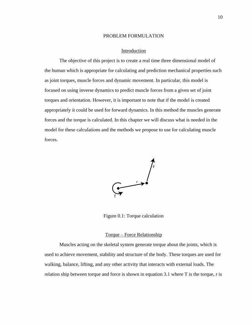
Figure 0.1: Torque calculation

Torque – Force Relationship

Muscles acting on the skeletal system generate torque about the joints, which is

used to achieve movement, stability and structure of the body. These torques are used for

walking, balance, lifting, and any other activity that interacts with external loads. The

relation ship between torque and force is shown in equation 3.1 where T is the torque, r is

11

a vector pointing from the where the torque is being calculated to where the force is being

applied and F is the applied force (Figure 0.1).

FrT ×= (3.1)

As an example, consider a simple beam attached to a fixed surface by a 1 DOF

hinge joint as shown in Figure 0.2. In this example we will consider the joint to be ideal

(frictionless) and the beam to be weightless. If r is given as [4.70, -1.71, 0] and F is

given as [2.59, 9.66, 0] then the torque can be calculated as

[ ] [ ] [ ]NmFrT 83.49,0,00,66.9,59.20,71.1,70.4 =×−=×= (3.2)

Figure 0.2: Example of the force-torque relationship

Figure 0.3: Example of multiple forces creating torque

12

Therefore, 49.83 Nm of torque is being developed about the z-axis of the hinge.

Now lets consider that we want to create 75 Nm of torque about the hinge. If the force

and the bar are still oriented in the same direction, what will the magnitude of the force

need to be? This can be found as

( ) NFFFT 05.15]98.4,0,0[]0,97.0,26.0[]0,71.1,70.4[]75,0,0[ =→=×−== (3.3)

If multiple forces were to act on the bar to total torque generated will simply be a

sum of the torque contributed by each force. Consider the above example but add another

force as shown in Figure 0.3. The torque about the hinge is now calculated by

NmFrFrTTT ]32.63,0,0[]83.49,0,0[]49.13,0,0[221121 =+=×+×=+= (3.4)

So, these two forces create 63.32 Nm of torque about the hinge.

Application of the Torque-Force Relationship to the Body

In this section we will take the torque-force relationship described in the previous

section and demonstrate how it is applied to the human body.

Figure 0.4: Major muscles of the upper arm

13

Musculoskeletal System

The musculoskeletal system is composed of the skeletal system and the skeletal

muscles. This system of muscles and bones is arranged throughout the body as numerous

levers where the bones act as the levers with the joints between them being the fulcrums.

Consider the muscles shown in Figure 0.4. This figure represents some of the major

muscles of the upper arm and illustrates how they are attached to the skeletal system.

Since muscles can only act in tension, each joint requires one set of muscles to

create a positive torque and a separate set to create negative torque. In Figure 0.4, the

elbow extension and flexion muscle groups are identified.

Mechanical System

Consider the simple one muscle model shown in Figure 0.5, which represents the

medial head of the bicep. This muscle originates on the scapula and inserts below the

elbow on the radius. For this simple example only the torque created at the elbow will be

considered. When the muscle is activated it creates a force on the radius. For this simple

example it will be assumed that this force points at the muscle origin (Figure 0.6). This

force creates a torque about the elbow by acting on a moment arm that lies along the

radius.

Figure 0.5: Medial bicep brachii

14

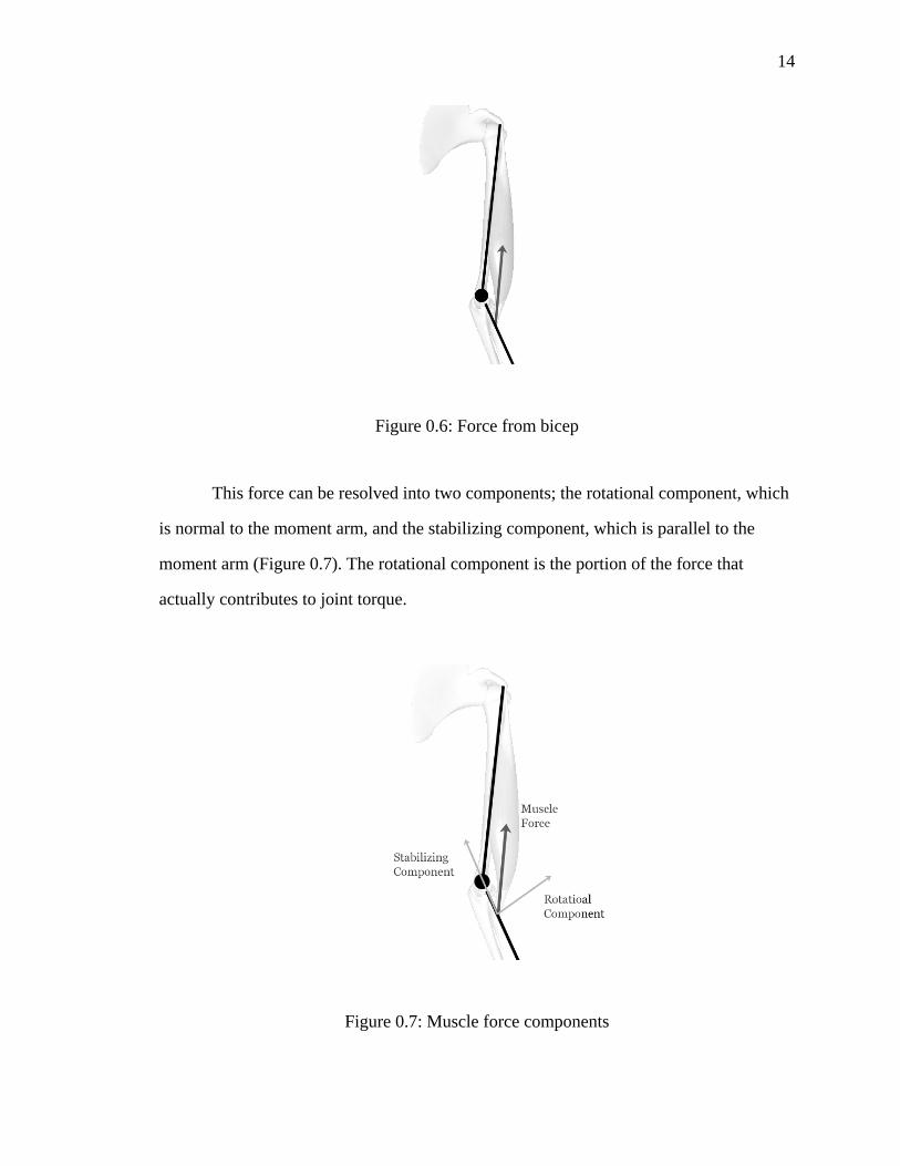
Figure 0.6: Force from bicep

This force can be resolved into two components; the rotational component, which

is normal to the moment arm, and the stabilizing component, which is parallel to the

moment arm (Figure 0.7). The rotational component is the portion of the force that

actually contributes to joint torque.

Figure 0.7: Muscle force components

15

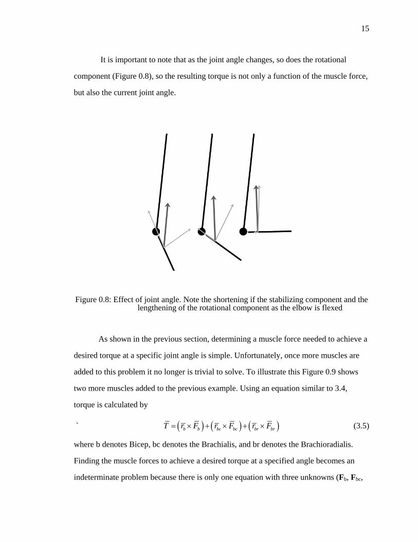
It is important to note that as the joint angle changes, so does the rotational

component (Figure 0.8), so the resulting torque is not only a function of the muscle force,

but also the current joint angle.

Figure 0.8: Effect of joint angle. Note the shortening if the stabilizing component and the lengthening of the rotational component as the elbow is flexed

As shown in the previous section, determining a muscle force needed to achieve a

desired torque at a specific joint angle is simple. Unfortunately, once more muscles are

added to this problem it no longer is trivial to solve. To illustrate this Figure 0.9 shows

two more muscles added to the previous example. Using an equation similar to 3.4,

torque is calculated by

` ( ) ( ) ( )b b bc bc br brT r F r F r F= × + × + × (3.5)

where b denotes Bicep, bc denotes the Brachialis, and br denotes the Brachioradialis.

Finding the muscle forces to achieve a desired torque at a specified angle becomes an

indeterminate problem because there is only one equation with three unknowns (Fb, Fbc,

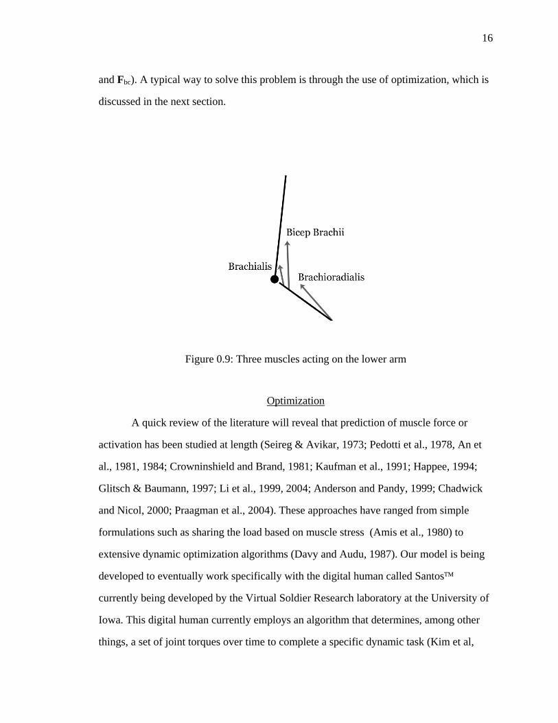
16

and Fbc). A typical way to solve this problem is through the use of optimization, which is

discussed in the next section.

Figure 0.9: Three muscles acting on the lower arm

Optimization

A quick review of the literature will reveal that prediction of muscle force or

activation has been studied at length (Seireg & Avikar, 1973; Pedotti et al., 1978, An et

al., 1981, 1984; Crowninshield and Brand, 1981; Kaufman et al., 1991; Happee, 1994;

Glitsch & Baumann, 1997; Li et al., 1999, 2004; Anderson and Pandy, 1999; Chadwick

and Nicol, 2000; Praagman et al., 2004). These approaches have ranged from simple

formulations such as sharing the load based on muscle stress (Amis et al., 1980) to

extensive dynamic optimization algorithms (Davy and Audu, 1987). Our model is being

developed to eventually work specifically with the digital human called Santos™

currently being developed by the Virtual Soldier Research laboratory at the University of

Iowa. This digital human currently employs an algorithm that determines, among other

things, a set of joint torques over time to complete a specific dynamic task (Kim et al,

17

2005). Because dynamic motion is already incorporated into these joint torques, we are

not concerned with muscle prediction algorithms that include dynamics. Additionally,

real time interaction is desired so we decided to initially develop this model with a simple

static optimization algorithm.

Solving this problem with optimization requires a cost function that will be

minimized while obeying various constraints. There have been many cost functions

proposed and choosing the most appropriate function is likely dependent on the situation.

For example, quick movement to avoid a collision will likely require a different cost

function than a movement that needs to be precise and smooth. For very strenuous

activities, Crowninshield found that minimizing the sum of the muscle stresses while

imposing constraints on how high the stresses can become predicted data the correlated

well with EMG signals (Crowninshield, 1978). Pedotti et al minimized equation 3.6

where fmax was calculated from instantaneous muscle length and muscle velocity of the

shortening and found a correlation with muscles associated with human gait.

∑ ⎟⎟⎠

⎞⎜⎜⎝

⎛=

2

maxif

fU i (3.6)

Crowninshield and Brand later presented equation 3.7 as a cost function where PCSA is

the physical cross sectional areas (Crowninshield and Brand, 1981). According to their

report, this formulation seems to be good for describing activities, which require

prolonged endurance.

3

∑ ⎟⎟⎠

⎞⎜⎜⎝

⎛=

i

i

PCSAfU (3.7)

Many cost functions use muscle activation as variables. Muscle activation is a

value that ranges between 0 and 1 where 0 indicates no muscle activation and 1 indicates

a fully activated muscle. Muscle force can then be defined as

F = a*Fmax (3.8)

18

where a is the activation and Fmax is the maximum theoretical force that muscle can

generate, which can estimated by the muscle’s physical cross sectional area. Torque can

now be represented as

( )max*T r a F= × (3.9)

To simplify the problem, only the torque being generated about the rotational axis of the

elbow will be considered. This allows the torque equation to become

T = r*a* Fmax (3.10)

where r is a constant and Fmax is the rotational component of Fmax. One way this problem

can now be solved is with the following optimization formulation where n is the number

of muscles being considered. Note that this formulation is similar to equation 3.6

Design Variables: a1 … an (3.11)

Minimize: ∑=

=n

iiaJ

1

2 (3.12)

Subject To: ∑=

=n

iiii FarT

1

)max( (3.13)

10 ≤≤ ia (3.14)

Note that by simply adding more torque equation constraints this formulation can

be expanded to cover numerous joints. It should be emphasized that is not our motivation

to determine which cost function is the best but simply create a real time model that can

work with many different formulations so that the user can determine which formulations

they would prefer to use. To illustrate how the muscle forces are predicted using

optimization an example will be presented.

Optimization Example

For this example, ten muscles will be considered. These muscles are the

brachialis, brachioradialis, bicep long, bicep short, tricep lateral, tricep long, tricep

19

medial, pronator teres, supinator, and anconeus. These muscles are used to flex/extend

the forearm and pronate/supinate the hand. Torque about the elbow and the pronating axis

of the wrist are given and the orientation of these joints is known. The objective is to find

the muscle activation level of the ten muscles listed above. This will be accomplished

through optimization as described in the previous section. For this example, the problem

is formulated as follows:

Design Variables: a1…a10

Minimize: 10

2

1i

iJ a

=

= ∑

Subject To: 1BR BL BS PT SUPT T T T T+ + + + =

10BR BCH BL BS TLAT TLON TM PT SUP ANCT T T T T T T T T T+ + + + + + + + + =

0 1ia≤ ≤

Where Tx is the torque generated by that muscle. Note that for this problem, it is

given that the torque about the wrist is 1 Nm and the torque about the elbow is 10 Nm. It

should also be noted that while all the muscle considered contribute some torque to the

elbow, only five contribute torque to the pronation of the hand.

Next the torque generated by each muscle must be calculated. These are

calculated as

maxi i i i iT r x a f= (3.15)

where r is the moment arm, x is the rotational component of the unit vector representing

the force line, a is the activation level, and fmax is the theoretical maximum isotonic force

which that muscle can create. The maximum isotonic force can be calculated by

multiplying the maximum physiological achievable muscle stress (600 kPa) to the

physiological cross sectional area (PSCA) of the muscle (Berme et al., 1987). The torque

equation can then be represented as

*600i i i i iT r x a PSCA= (3.16)

20

Note that r and PSCA are constants while x is dependent on the joint angles and a

is the design variable. Since the joint angles are known, x can be calculated from

geometry while r and PSCA can be found in literature (Maurel and Thalmann, 1999),. For

example, TBR about the elbow can be calculated as

0.0662*0.424* *4.70*600 14.149BRT a a= = (3.17)

So, for the given orientation, the constraint equations can be calculated as

2 3 4 8 90.002 1.281 1.112 ( 0.724) 0.025 1a a a a a+ + + − + = (3.18)

1 2 3 4 5 6 7

8 9 10

14.149 8.670 4.833 4.228 ( 2.640) ( 2.617) ( 2.636)1.230 4.012 0.0112 10

a a a a a a aa a a+ + + + − + − + −

+ + + =(3.19)

Solving the optimization problem in Excel predicts the following activation

levels for each muscle.

• Bracialis: 0.303

• Brachioradialis: 0.186

• Bicep Long: 0.445

• Bicep Short: 0.384

• Tricep Lateral: 0

• Tricep Long: 0

• Tricep Medial: 0

• Pronator Teres: 0

• Supinator: 0.093

• Anconeus: 0

As expected none of the triceps are active because positive torque about the elbow

is required. Similarly, the pronator teres is not active because it will contribute negative

torque about the pronation axis while positive torque is required.

21

Proposed Formulation

Our proposed formulation is quite similar to the example previously presented

except it will incorporate two more joints and 34 action lines representing the muscles of

the arm and shoulder. The problem is defined as follows.

Design Variables: a1…a34

Minimize: ∑=

=34

1

2

iiaJ

Subject To:

SCSC

DorsiUpperLatissimusSC

eDorsiMiddlLatissimusSC

DorsiLowerLatissimusSC

MajorLowerPectoralis

SCMajorUpperPectoralis

SCMinorPectoralis

SCrteriorUppeSerratusAn

SCleteriorMiddSerratusAn

SCrteriorLoweSerratusAn

SCboidsMinorR

SCboidsMajorR

SCpperTrapeziusU

SCiddleTrapeziusM

SCowerTrapeziusL

SCpulaeLevatorSca

TTTTT

TTTTT

TTTTTT

=++++

+++++

+++++ homhom

GHGH

TricepLongGH

BicepLongGH

DorsiLowerLatissimisGH

eDorsiMiddlLatissimis

GHDorsiUpperLatissimis

GHTeresMajor

GHTeresMinor

GHrisSubscapula

GHtusInfraspina

GHateralDeltoidusL

GHnteriorDeltoidusA

GHosteriorDeltoidusP

GHtusSupraspina

GHhialisCoracobrac

GHMajorLowerPectoralis

GHMajorUpperPectoralis

TTTTT

TTTTTT

TTTTTT

+=++++

++++++

+++++

UHzUHz

AnconeusUHzSupinator

UHzSupinator

UHzsonatorTere

UHzialisBrachiorad

UHzralTricepLate

UHzalTricepMedi

UHzTricepLong

UHzBrachialis

UHzBicepShort

UHzBicepLong

TTTTT

TTTTTTT

+=++++

++++++

21Pr

URzURzSupinator

URzsonatorTere

URzdialisBracchiora

URzBicepShort

URzBicepLong TTTTTT =++++ 1Pr

0 1ia≤ ≤ for i=1 to 34

In the above formulations xyT is the torque that muscle y creates about joint x,

which is calculated from equation 3.9. Note that the torques about SC and GH are vectors

while the torques about UH and UR are only considering the torque about the z axis. It

should also be noted that only the torque about the x and z axis of the SC joint will be

considered. Additionally, one can see that torque about the AC joint is not a constraint.

This was decided because normal movement of the shoulder is primarily the rotation of

GH joint about all three of its axes and the rotation of the SC about it’s x and z axes. Any

22

movement about the AC joint is assumed to be used to keep the scapula on the thorax and

rotation of the clavicle about the y axis of the SC joint is considered to be negligible.

Model Requirements

By observing the above formulation for predicting muscle activation levels it can

be observed that two variables will come from the 3D model representing the arm,

regardless of the cost function used. These are the r vector and the direction of the force

vector. Therefore it is imperative that the model be created with careful consideration for

where the muscles originate and insert. It is also important that the action lines of the

muscles be accurate so that the direction of the force being predicted is realistic. This is

complicated by the requirement that the model be interactive in real time. The

development of the model will be addressed in the next chapter. Real time wrapping will

be used to keep the action lines of the muscles in a realistic position, which will be

detailed in chapter 5.

23

MODELING

Introduction

The human body is a complex arrangement of numerous biological systems all

working together in multifarious relationships that science has yet to fully understand. In

this chapter we will explore some of the systems used for motion and then present our

method for creating a real time interactive representation of the human arm. The model

being developed is designed explicitly for prediction of muscle activation levels through

inverse dynamics. Because we are interested in movement, the two main systems of

interest are the skeletal and muscular system and the interaction between them.

Anatomy

The skeletal system is composed of 206 bones, which are divided into two groups,

the axial and the appendicular (Figure 0.1).

Figure 0.1: Axial skeleton (left) and appendicular skeleton (right)

24

The axial system is composed of the skull, spine and ribs while the appendicular

is composed of the limbs and the girdles that connect them to the trunk. The bones are

linked to each other with ligaments to form joints or articulations. It is this arrangement

of bones that give humans their structure. However, it is the muscles acting on the bones

that hold together and move this structure. Skeletal muscles, which are attached to either

a bone via a tendon or to other muscles with aponeuroses, provide tensile force to the

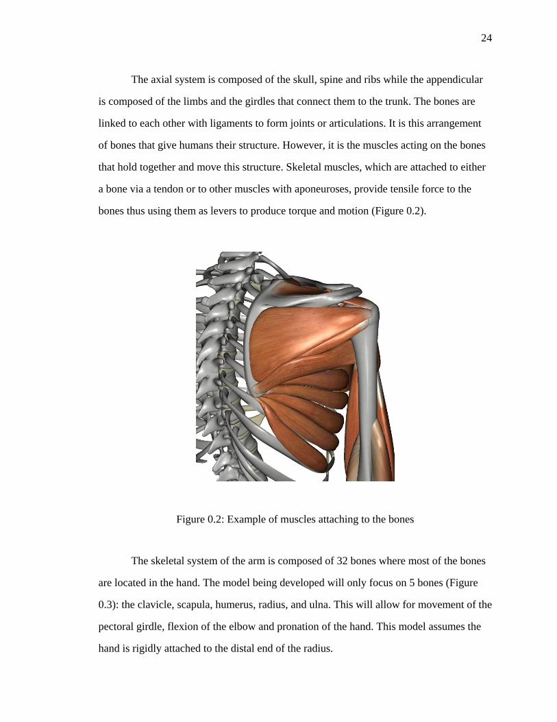
bones thus using them as levers to produce torque and motion (Figure 0.2).

Figure 0.2: Example of muscles attaching to the bones

The skeletal system of the arm is composed of 32 bones where most of the bones

are located in the hand. The model being developed will only focus on 5 bones (Figure

0.3): the clavicle, scapula, humerus, radius, and ulna. This will allow for movement of the

pectoral girdle, flexion of the elbow and pronation of the hand. This model assumes the

hand is rigidly attached to the distal end of the radius.

25

Figure 0.3: Bones of the right arm

These movements are accomplished through the rotation of five articulations.

Starting proximally, the first joint is between the scapula and the clavicle. This joint is

called the sterno-clavicular (SC) joint. The next joint is the acromio-clavicular (AC) joint,

which is the interaction between the clavicle and the scapula. The gleno-humeral (GH)

joint between the humerus and the scapula comes next followed by the ulno-humeral

(UH) joint between the unla and humerus. Last is the ulno-radial (UR) joint between the

ulna and radius, which allows for the pronation of the hand.

Our model considers 21 muscles important for the manipulation of the above

joints based on anatomical analysis. They are

• Levator Scapulae: This muscle has four functions, elevation of the

scapula, rotation of the scapula to tilt the glenoid cavity inferiorly,

retraction of the scapula, and lateral flexion of the neck (Figure 0.5).

26

Figure 0.4: Muscles of the shoulder

• Trapezius: This muscle also has four functions, elevation of the scapula,

retraction of the scapula, depression of the scapula, and superior rotation

of the scapula (Figure 0.4).

• Rhomboids: This muscle has two functions, retraction of the scapula and

rotation of the scapula to depress the glenoid cavity (Figure 0.5).

• Serrratus Anterior: This muscle has two functions, protraction of the

scapula and rotation of the scapula (Figure 0.5 and Figure 0.6).

• Pectoralis Minor; This muscle has two function, inferior drawing of the

scapula and anterior drawing of the scapula (Figure 0.6).

• Pectoralis Major: This muscle has two functions, flexion of the humerus

and adduction and medial rotation of the humerus (Figure 0.7).

27

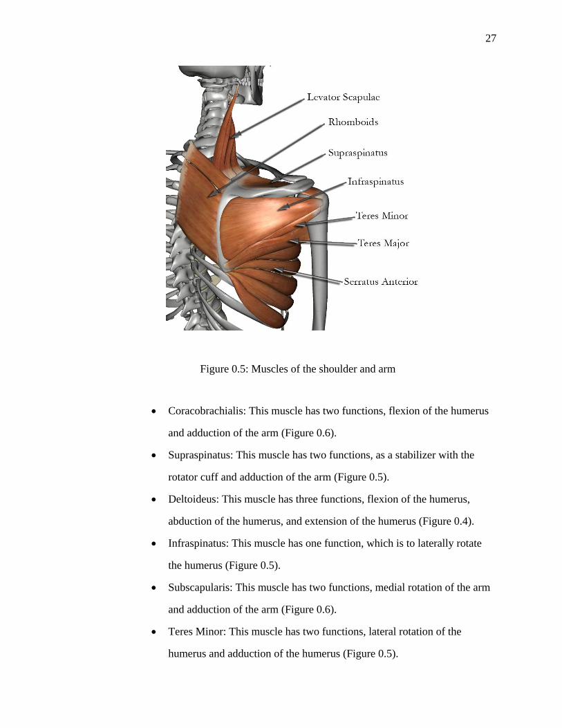
Figure 0.5: Muscles of the shoulder and arm

• Coracobrachialis: This muscle has two functions, flexion of the humerus

and adduction of the arm (Figure 0.6).

• Supraspinatus: This muscle has two functions, as a stabilizer with the

rotator cuff and adduction of the arm (Figure 0.5).

• Deltoideus: This muscle has three functions, flexion of the humerus,

abduction of the humerus, and extension of the humerus (Figure 0.4).

• Infraspinatus: This muscle has one function, which is to laterally rotate

the humerus (Figure 0.5).

• Subscapularis: This muscle has two functions, medial rotation of the arm

and adduction of the arm (Figure 0.6).

• Teres Minor: This muscle has two functions, lateral rotation of the

humerus and adduction of the humerus (Figure 0.5).

28

Figure 0.6: Muscles of the shoulder and arm

• Teres Major: This muscle has two functions, adduction of the arm and

medial rotation of the humerus (Figure 0.5).

• Latissimus Dorsi: This muscle has three functions, medial rotation of the

arm, extension of the humerus, and adduction of the humerus (Figure

0.4).

• Bicep Brachii: This muscle has two functions, flexion of the forearm and

supination of the forearm (Figure 0.7)..

• Brachialis: This muscle has one function, which is flexion of the forearm

(Figure 0.7).

• Triceps Brachii: These muscles have two functions, extension of the

forearm and adduction of the arm (Figure 0.8).

29

Figure 0.7: Muscles of the shoulder and arm

• Brachioradialis: This muscle has tow functions, flexion of the forearm

and supination of the forearm (Figure 0.7).

• Pronator Teres: This muscle has one function, which is to pronate the

forearm (Figure 0.7).

• Supinator: This muscle has one function, which is to supinate the forearm

(Figure 0.8).

• Anconeus: This muscle has one function, which is to extend the forearm

(Figure 0.8).

Digital Representation of the Arm

The purpose of this model is to predict muscle activation levels based from a

given limb configuration to achieve specified joint torques. The torque achieved by the

30

Figure 0.8: Muscles of the arm

muscles pulling on the bones in lever like arrangements. Therefore it is imperative that

the kinematic model of bones as well as the attachment points and direction of the

muscles be as realistic as possible. To accomplish this many geometric models of the

musculoskeletal system were examined before one was selected. The model selected is

commercially available and was created with careful consideration to true human

anatomy. Once the model was obtained, it was translated to VRML and then imported

into our real time simulation environment. The model contained all the bones and

muscles in the human body. All the bones were removed except for the ribs, sternum,

spine, and bones of the right arm. All the muscles were deleted except for the ones listed

in the previous section, and these were kept for the right arm only.

31

Kinematic Model

Once the appropriate geometric model was imported into the simulation, the

bones had to be arranged into an appropriate kinematic chain. A kinematic chain is

essentially a series of rigid bodies connects by joints. This was accomplished by first

arranging the bones in the appropriate hierarchy. A parent-child relationship is essential

when created a kinematic chain. In this type of relationship, each part can have only one

parent but numerous children. Movement of an object within the hierarchy will affect its

children but not the parent. The ribs, sternum and spine were grouped together and

considered to be the base of the kinematic chain, thus have no parent. The rest of the

bones were arranged the hierarchy shown in Figure 0.9. Because of the hierarchy,

movement of the clavicle will affect all the distal bones in the arm but movement of the

radius will only affect the hand.

Figure 0.9: Hierarchy of the bones in the arm

Once the hierarchy of bones was created the joints between the bones had to be

defined. In a true human joint, most movement is a combination of rolling and sliding

between the bones (Engin, 1984), thus no fixed axis or center of rotation can be found.

However, this movement is generally considered negligible for the arm, so the joints are

modeled either as an ideal ball and socket joint with three degrees of freedom or a hinge

joint with one degree of freedom. Following previous kinematic arm models (Maurel and

32

Thalmann, 1999; Engin, 1980; Helm, 1994; Hogfors et al, 1987; Raikova, 1992) the SC,

AC, and GH joints are modeled as ball and sockets while the UH and UR are modeled as

hinge joints (Figure 0.10).

Figure 0.10: Joints of the arm

One of the more difficult features about modeling the shoulder is how to treat the

scapula and its interaction with the thorax. The scapula is located between the clavicle

and the humerus in the kinematic chain and is constrained to glide across the thorax (Dvir

and Berme, 1978). Because the scapula is nearly completely surrounded by soft tissues,

there are no articular structures between the scapula and the thorax, resulting in the

scapula being able to move in all six degrees of freedom. Since the scapula glides across

the thorax two forms have been proposed to describe this constraint, a dot contact or a

33

linear contact (Maurel and Thalmann, 1999). A dot constraint describes a situation when

one point of an object is constrained to a surface, thus allowing 5DOF. A line constraint

describes a situation when two points of an object are constrained to surface resulting in

4DOF. It was decided that the linear contact constraint is more representative of

movement of the shoulder as described by Dvir and Berme but instead of using an

idealized ellipsoidal thorax as van der Helm did we used the actual geometric model of

the thorax. (Helm, 1994)

Figure 0.11: Guide points on the scapula

To accomplish this we started by first location two frames on the medial edge of

the scapula with their x-axis pointing towards the thorax. These points will be called g1

and g2. A ray is cast along each of the frames x-axis to determine the distance between

the frame and the thorax. Then the scapula is rotated about the SCy until the distance

between g1 and the thorax is within a certain range (Figure 0.12). Then the scapula is

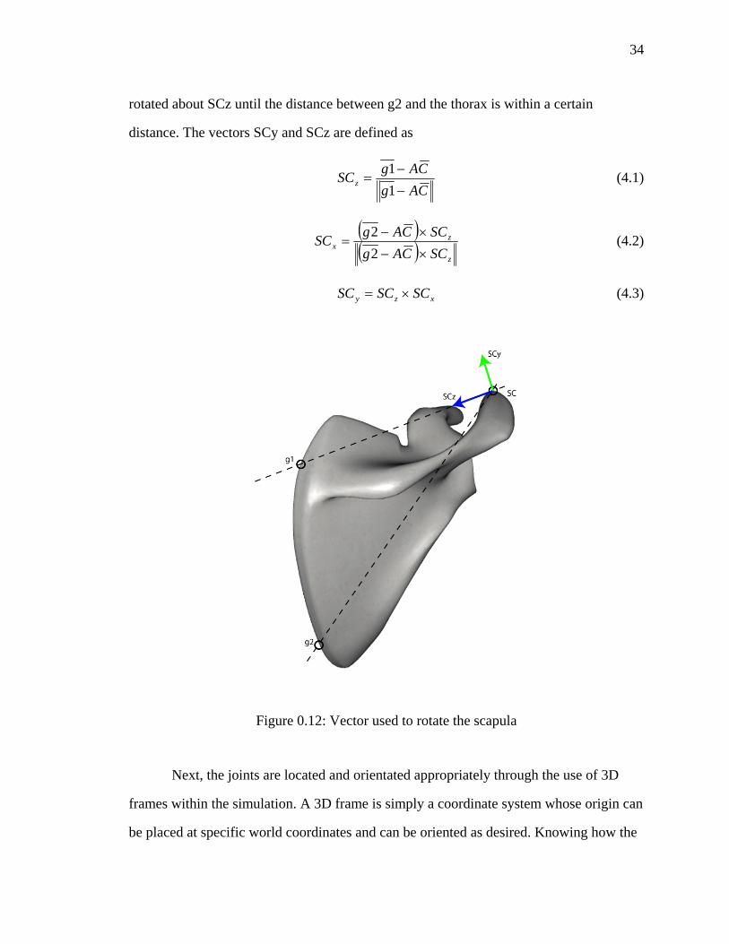
34

rotated about SCz until the distance between g2 and the thorax is within a certain

distance. The vectors SCy and SCz are defined as

CAgCAgSCz

−−

=11 (4.1)

( )( ) z

zx

SCCAgSCCAgSC

×−

×−=

22 (4.2)

xzy SCSCSC ×= (4.3)

Figure 0.12: Vector used to rotate the scapula

Next, the joints are located and orientated appropriately through the use of 3D

frames within the simulation. A 3D frame is simply a coordinate system whose origin can

be placed at specific world coordinates and can be oriented as desired. Knowing how the

35

rotations are going to be described is directly related to how the joint frames will be

placed and oriented. There are many methods for describing how the bones articulate

including bone or joint rotation, global or local coordinates, and local or virtual

references (Helm and Pronk, 1995). The goal of this model is to predict muscle activation

levels from a given torque and joint configuration, which is given as absolute joint

Figure 0.13: Heirarchy of joint frames in a 3DOF joint

Figure 0.14: Euler rotation order for a 3DOF joint. Note that all the frames are separated just for clarity. In the model they coincide.

36

rotation in local coordinates. Therefore, our model will use joint angles defined in the

coordinate system of the parent bone, which requires a reference frame on the bone

proximal to the joint and a local frame, which will actually be rotated. Following the

model presented by Maurel et al our rotations will be described as Euler angles defined to

rotate in the following order: θ about z, φ about y, and ψ about x (Maurel et al, 1996). To

accomplish this in our simulation instead of using a single local frame, three frames are

stacked on top of each other and arranging in the hierarchy shown in Figure 0.13. Then to

achieve a specified orientation local frame 1 is rotated about it’s z-axis by θ, local frame

2 is rotated about it’s y axis by φ, and local frame 3 is rotated about it’s x axis by ψ

(Figure 0.14).

The position of the frames within the simulation was based on the geometric

model and understanding the action of that joint while the frames were oriented based on

a combination of data from literature and observation of the geometric models (Maurel

and Thalman, 1999). For example, the GH joint was positioned in the approximate center

of the head on the humerus. The absolute reference frame for the simulation was oriented

such that Xo is perpendicular to the front plane and the Yo is perpendicular to the side

plane. The rest of the joints were orientated as follows

• Sterno-Clavicular: The reference frame is attached to the sternum and

oriented such that the x is perpendicular to the front plane pointing

forward and the y is perpendicular to the side plane, pointing to the left.

The local frame is attached to the clavicle and orientated such that the y is

a unit vector pointing from the SC to the AC joint and the x is

perpendicular to the y-axis and pointing forward in the clavicular plane

(Figure 0.15).

• Acromio-Clavicular: The reference frame is attached to the clavicle and

orientated such that x is a unit vector pointing from the SC to the AC joint

while the y is perpendicular to the x axis and pointing backwards in the

37

clavicular plane. The local frame is attached to the scapula and is

orientated such that y is perpendicular to the scapluar plane pointing

backwards while the x is aligned with the trigonum spinae of the scapula

(Figure 0.16).

Figure 0.15: Sterno-clavicular reference (left) and local frame (right)

Figure 0.16: Acromio-clavicular reference (left) and local frame (right)

38

• Gleno-Humeral: The reference frame is attached to the scapula with it’s z

perpendicular to the scapular plane pointing forward while the x is aligned

with the trigonum spinae. The local is attached to the humerus with the z

perpendicular to the humeral front plane pointing forward and the y

pointing up along the humeral axis (Figure 0.17).

Figure 0.17: Gleno-humeral reference (left) and local frame (right)

Figure 0.18: Ulno-humeral reference and local frame

39

• Ulno-Humeral: The reference frame is attached to the humerus with the z

as a unit vector pointing from the UH to the HR joint and the x set normal

to a plane created by GH, HR, and UR, pointing forward. The local axis.

The local frame is attached to the ulna and orientated the same as the

reference (Figure 0.18).

Figure 0.19: Ulno-radial reference and local frame

• Ulno-Radial: The reference frame is attached to the ulna and oriented so

the z is a unit vector pointing from the UR to HR while y is normal to a

plane created by HR, UR, and the end of the radius, pointing inward. The

local is attached to the radius and is orientated the same as the reference

(Figure 0.19).

Attaching the Muscles

When attaching the muscles to the kinematic model, two factors are of great

importance. The first is the shape of the muscle, which is dependent on where it attaches

40

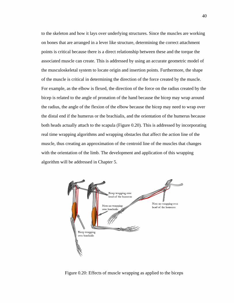
to the skeleton and how it lays over underlying structures. Since the muscles are working

on bones that are arranged in a lever like structure, determining the correct attachment

points is critical because there is a direct relationship between these and the torque the

associated muscle can create. This is addressed by using an accurate geometric model of

the musculoskeletal system to locate origin and insertion points. Furthermore, the shape

of the muscle is critical in determining the direction of the force created by the muscle.

For example, as the elbow is flexed, the direction of the force on the radius created by the

bicep is related to the angle of pronation of the hand because the bicep may wrap around

the radius, the angle of the flexion of the elbow because the bicep may need to wrap over

the distal end if the humerus or the brachialis, and the orientation of the humerus because

both heads actually attach to the scapula (Figure 0.20). This is addressed by incorporating

real time wrapping algorithms and wrapping obstacles that affect the action line of the

muscle, thus creating an approximation of the centroid line of the muscles that changes

with the orientation of the limb. The development and application of this wrapping

algorithm will be addressed in Chapter 5.

Figure 0.20: Effects of muscle wrapping as applied to the biceps

41

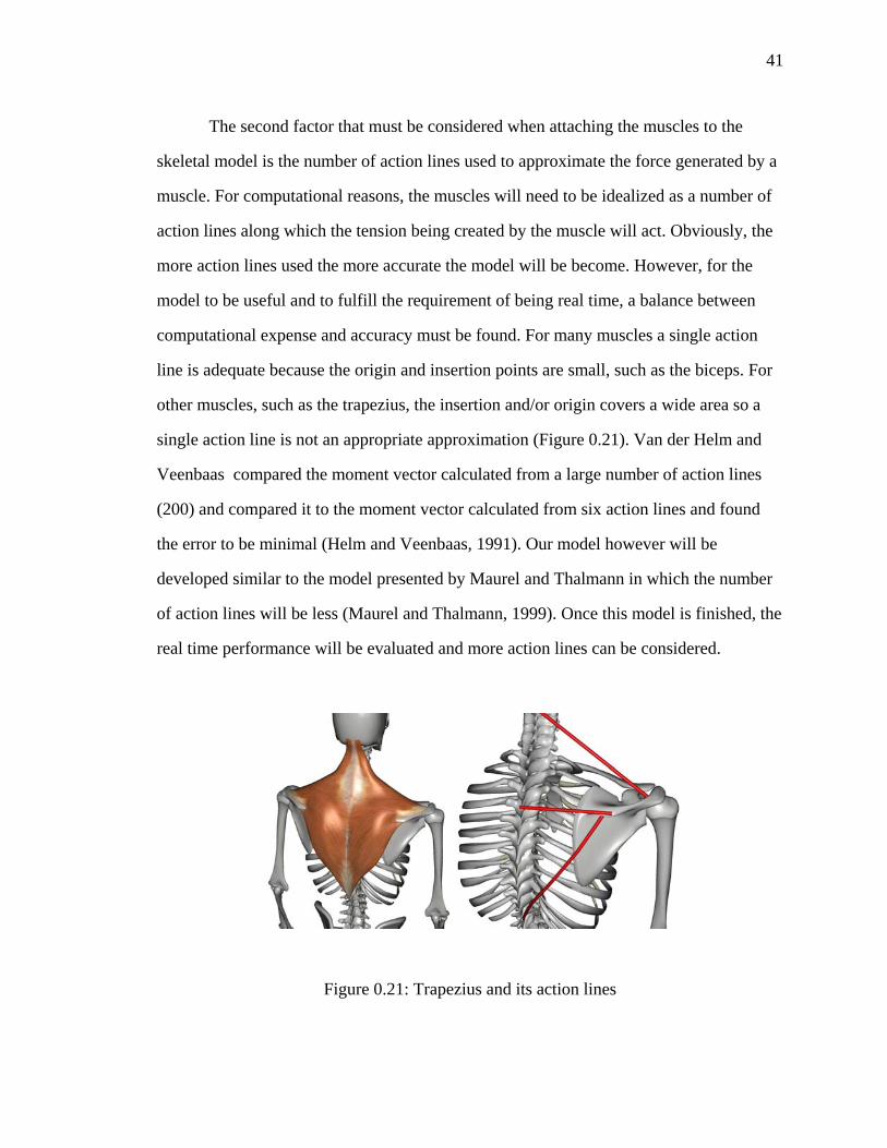
The second factor that must be considered when attaching the muscles to the

skeletal model is the number of action lines used to approximate the force generated by a

muscle. For computational reasons, the muscles will need to be idealized as a number of

action lines along which the tension being created by the muscle will act. Obviously, the

more action lines used the more accurate the model will be become. However, for the

model to be useful and to fulfill the requirement of being real time, a balance between

computational expense and accuracy must be found. For many muscles a single action

line is adequate because the origin and insertion points are small, such as the biceps. For

other muscles, such as the trapezius, the insertion and/or origin covers a wide area so a

single action line is not an appropriate approximation (Figure 0.21). Van der Helm and

Veenbaas compared the moment vector calculated from a large number of action lines

(200) and compared it to the moment vector calculated from six action lines and found

the error to be minimal (Helm and Veenbaas, 1991). Our model however will be

developed similar to the model presented by Maurel and Thalmann in which the number

of action lines will be less (Maurel and Thalmann, 1999). Once this model is finished, the

real time performance will be evaluated and more action lines can be considered.

Figure 0.21: Trapezius and its action lines

42

With the above factors considered, the muscles were modeled as follows.

• Levator Scapulae: This muscle was modeled as a single line running from

the neck to the medial border of the scapula. No wrapping obstacles were

included (Figure 0.22).

Figure 0.22: Levator scapulae muscle and action line

Figure 0.23: Trapezius muscle, action lines and wrapping obstacles

43

• Trapezius: Modeled as three action lines. The first one originated at the

neck and inserted near the AC joint on the scapula. No wrapping was

included for this action line. The second action line originates at the upper

thoracic vertebra and insets on the spine of the scapula. It requires one

wrapping obstacle that is a cylinder for the thorax. The third action line

originates at the lower thoracic vertebra and inserts on the spine of the

scapula. It requires two wrapping obstacles, one cylinder for the thorax

and one cylinder for the medial spine of the scapula (Figure 0.23).

t

Figure 0.24: Rhomboid muscles, action lines and wrapping obstacle

• Rhomboids: Modeled as two action lines, both of which originate on the

spine, insert on the posterior side of the scapula and require a cylinder

obstacle for wrapping around the thorax (Figure 0.24).

• Serrratus Anterior: Modeled as three action lines, all of which originate

on the ribs, insert on the anterior side of the scapula and require a cylinder

obstacle for wrapping around the thorax (Figure 0.25).

44

Figure 0.25: Serratus anterior muscles, action lines and wrapping obstacles

Figure 0.26: Pectoralis minor muscle, action lines and wrapping obstacle

• Pectoralis Minor: Modeled as a singe action line, which originates on the

ribs, inserts on the coracoid process of the scapula and requires a cylinder

obstacle for wrapping around the thorax (Figure 0.26).

• Pectoralis Major: Modeled as two action lines, both of which originate on

the sternum and insert on the humerus. Both require a cylinder obstacle

for wrapping around the thorax and a second cylinder obstacle for

wrapping around the humerus (Figure 0.27).

45

Figure 0.27: Pectoralis major muscle, action lines and wrapping obstacles

Figure 0.28: Coracobrachialis muscle, action line and wrapping obstacle

• Coracobrachialis: Modeled as a singe action line, which originates on the

scapula, inserts on the humerus and requires a cylinder obstacle for

wrapping around the humerus (Figure 0.28).

• Supraspinatus: Modeled as a singe action line, which originates on the

scapula above the spine, inserts on the humeral head and requires a

spherical obstacle for wrapping around the head of the humerus (Figure

0.29).

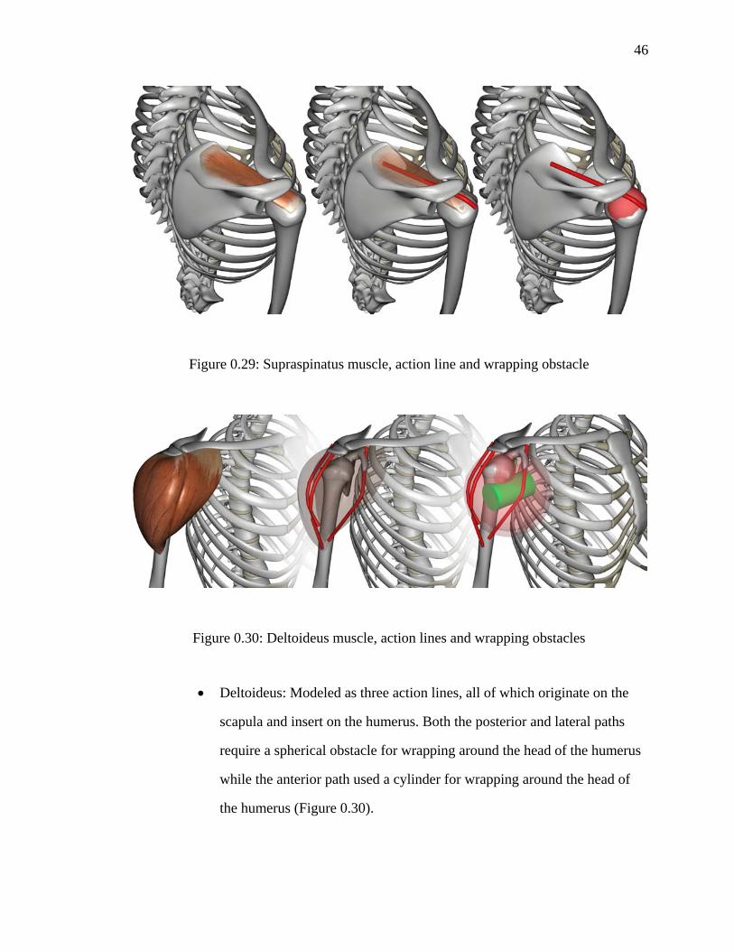
46

Figure 0.29: Supraspinatus muscle, action line and wrapping obstacle

Figure 0.30: Deltoideus muscle, action lines and wrapping obstacles

• Deltoideus: Modeled as three action lines, all of which originate on the

scapula and insert on the humerus. Both the posterior and lateral paths

require a spherical obstacle for wrapping around the head of the humerus

while the anterior path used a cylinder for wrapping around the head of

the humerus (Figure 0.30).

47

Figure 0.31: Infraspinatus muscle, action line and wrapping obstacle

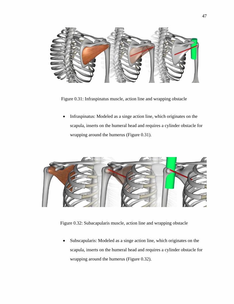
• Infraspinatus: Modeled as a singe action line, which originates on the

scapula, inserts on the humeral head and requires a cylinder obstacle for

wrapping around the humerus (Figure 0.31).

Figure 0.32: Subacapularis muscle, action line and wrapping obstacle

• Subscapularis: Modeled as a singe action line, which originates on the

scapula, inserts on the humeral head and requires a cylinder obstacle for

wrapping around the humerus (Figure 0.32).

48

Figure 0.33: Teres Minor muscle, action line and wrapping obstacles

• Teres Minor: Modeled as a single action line, which originate on the

scapula, insert on the humeral head. It requires a cylinder obstacle for

wrapping around the humerus and a cylinder obstacle for wrapping over

the lateral spine of the scapula (Figure 0.33).

Figure 0.34: Teres Major muscle, action line and wrapping obstacles

49

• Teres Major: Modeled as a singe action line, which originates on the

scapula and inserts on the humeral head and requires a cylinder obstacle

for wrapping around the humerus (Figure 0.34).

Figure 0.35: Latissimus dorsi muscle, action lines and wrapping obstacles

• Latissimus Dorsi: Modeled as three action lines, two of which originate

on the spine and the third on the thorax. All three insert on the humerus.

All three paths require a cylinder for wrapping around the thorax and a

cylinder for wrapping around the humerus (Figure 0.35).

Figure 0.36: Bicep brachii muscles, action lines and wrapping obstacles

50

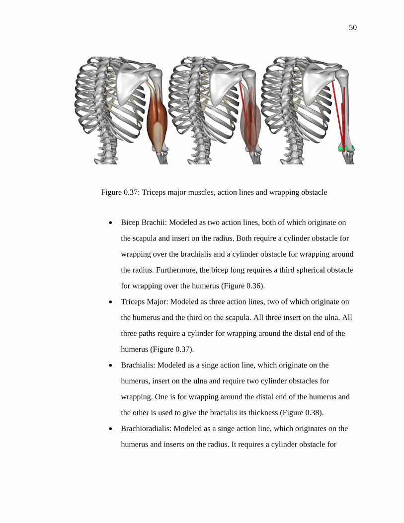
Figure 0.37: Triceps major muscles, action lines and wrapping obstacle

• Bicep Brachii: Modeled as two action lines, both of which originate on

the scapula and insert on the radius. Both require a cylinder obstacle for

wrapping over the brachialis and a cylinder obstacle for wrapping around

the radius. Furthermore, the bicep long requires a third spherical obstacle

for wrapping over the humerus (Figure 0.36).

• Triceps Major: Modeled as three action lines, two of which originate on

the humerus and the third on the scapula. All three insert on the ulna. All

three paths require a cylinder for wrapping around the distal end of the

humerus (Figure 0.37).

• Brachialis: Modeled as a singe action line, which originate on the

humerus, insert on the ulna and require two cylinder obstacles for

wrapping. One is for wrapping around the distal end of the humerus and

the other is used to give the bracialis its thickness (Figure 0.38).

• Brachioradialis: Modeled as a singe action line, which originates on the

humerus and inserts on the radius. It requires a cylinder obstacle for

51

wrapping around the distal end of the humerus and another cylinder for

wrapping over underlying structures in the forearm (Figure 0.39).

Figure 0.38: Brachialis muscle, action line and wrapping obstacles

Figure 0.39: Brachioradialis muscle, action line and wrapping obstacles

52

Figure 0.40: Pronator teres muscle, action line and wrapping obstacles

Figure 0.41: Supinator muscle, action lines and wrapping obstacles

• Pronator Teres: Modeled as a singe action line, which originates on the

humerus and inserts on the radius. It requires a cylinder obstacle for

53

wrapping around the distal end of the humerus and another cylinder for

wrapping over underlying structures in the forearm (Figure 0.40).

• Supinator: Modeled as two action lines, both of which originate on the

radius. One insert on the radius while the second inserts on the ulna. Both

require a cylinder obstacle for wrapping over the distal end of the

humerus and the one that inserts on the radius requires a second cylinder

obstacle for wrapping around the radius (Figure 0.41).

Figure 0.42: Anconeus muscle, action line and wrapping obstacle

• Anconeus: Modeled as a singe action line, which originate on the

humerus, insert on the ulna, and requires a cylinder obstacle for wrapping

around the distal end of the humerus (Figure 0.42).

As a result, 34 action line are used to model the 21 muscles considered. Nearly all

of these muscles require at least one wrapping obstical. The result is shown in

Figure 0.43.

54

Figure 0.43: All modeled action lines

Conclusion

This chapter presented the modeling of the 3D geometric representation of the

arm. This modeling included creating a kinematically correct hierarchy, attaching the

muscles in the appropriate location and placing obstacle as needed for the muscle to wrap

over. The next chapter will formulate the algorithms for allowing the action lines to wrap

over the obstacles.

55

MUSCLE WRAPPING MODEL

Introduction

The muscloskeletal system is a complex arrangement of muscles wrapping around

bones and other underlying muscles. When these muscles are actuated they create torque

about the joint or joints they cross because of the lever-like attachments. For example,

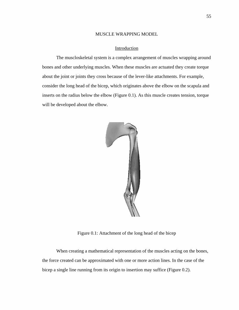
consider the long head of the bicep, which originates above the elbow on the scapula and

inserts on the radius below the elbow (Figure 0.1). As this muscle creates tension, torque

will be developed about the elbow.

Figure 0.1: Attachment of the long head of the bicep

When creating a mathematical representation of the muscles acting on the bones,

the force created can be approximated with one or more action lines. In the case of the

bicep a single line running from its origin to insertion may suffice (Figure 0.2).

56

Figure 0.2: Straight line model for the short head of the bicep

Seireg and Arvikar used this simple method of action line modeling in 1973 to

represent a large number of muscles in the leg. “The straight lines have to be chosen to

represent the best approximation for the lines of action in space of the muscular tensile

forces” (Seireg and Avikar, 1973). This simple model may be adequate for some muscles

in certain orientation, but is not nearly robust enough for a real time simulation that

allows the user to interactively orient the limb to any position within the prescribed joint

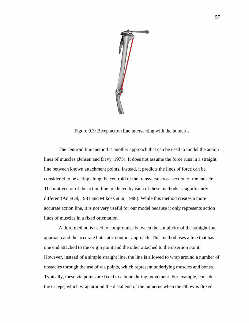
limits. For example, consider the bicep again. In the orientation shown in the Figure 0.1,

a straight line running from the insertion to the origin may be acceptable. However, if the

forearm is fully extended one will note that this same line now passes through the distal

end of the humerus (Figure 0.3). Not only is this physically impossible but any

calculation based on this model would be questionable. Many muscles can never be

modeled as a straight line from origin to insertion. For example, consider the deltoid,

which originates on the scapula and inserts on the humerus after curving over the gleno-

humeral joint. Because of the curved nature of this muscle, representing the action line as

one or more straight lines would be insufficient.

57

Figure 0.3: Bicep action line intersecting with the humerus

The centroid line method is another approach that can be used to model the action

lines of muscles (Jensen and Davy, 1975). It does not assume the force runs in a straight

line between known attachment points. Instead, it predicts the lines of force can be

considered to be acting along the centroid of the transverse cross section of the muscle.

The unit vector of the action line predicted by each of these methods is significantly

different(An et al, 1981 and Mikosz et al, 1988). While this method creates a more

accurate action line, it is not very useful for our model because it only represents action

lines of muscles in a fixed orientation.

A third method is used to compromise between the simplicity of the straight-line

approach and the accurate but static contour approach. This method uses a line that has

one end attached to the origin point and the other attached to the insertion point.

However, instead of a simple straight line, the line is allowed to wrap around a number of

obstacles through the use of via points, which represent underlying muscles and bones.

Typically, these via points are fixed to a bone during movement. For example, consider

the triceps, which wrap around the distal end of the humerus when the elbow is flexed

58

(Figure 0.4). A set of reasonable via points for modeling the force line of this muscle

would be fixed with respect to the humerus, thus keeping the action line out of the end of

the humerus. The only algorithm needed would be to determine which of the via points

are active. None of the via points will be active when the elbow is full extended and all

the via points will be active when the elbow if fully flexed.

Figure 0.4: Triceps action lines with fixed via points about the elbow

While this may work well for muscles that only crosses a joint with only one

degree of rotational freedom, fixed via points become a problem when more complex

wrapping must occur. For example, consider the force line shown in Figure 0.5 which

represents the lower action line of the trapezuis. This line originates in the thoracic

region of the spine, wraps around the thorax and the posterior surface of the scapula. The

movement of the scapula and shoulder affects the shape of this muscle. If one were to use

fixed via points the action line would not be allowed to slide over the medial edge of the

scapula during movement of the shoulder, thus producing an inaccurate approximation of

the muscles centroid line.

59

Figure 0.5: Lower action line of the trapezius with fixed via points on the medial edge of the scapula

This chapter will present a method for real time approximation of how muscles

will wrap around underlying structures by allowing floating via points to dynamically

wrap around prescribed obstacles. The difference between the floating via points and the

fixed via points is that the floating via points are not fixed to a bone but are allowed to

slide across the surface of the obstacle. This approach makes two assumptions about the

action lines. The first is that the action line or lines of a muscle can be modeled as a

frictionless elastic string wrapping around prescribed obstacles. The second is that

spheres and cylinders can represent the underlying anatomical structures that the muscle

must wrap around. The lines being wrapped will then be used to approximate the force

lines generated by the muscles.

Problem Formulation

We propose to develop an algorithm that uses prescribed obstacles to bend the

action line of a muscle in real time such that the action line is a reasonable approximation

of the real muscle’s action line for all possible joint configurations. From anatomy we

60

can determine the origin and insertion of a particular muscle. We can also analyze

underlying muscles and bones so as to determine the size, shape, position and number of

obstacles that the muscle being modeled must wrap around. Therefore, the unknowns are

the positions of the intermediate floating via points. These positions will be dependent on

two factors, if there are one or more obstacles about which wrapping should occur and, if

so, the shape and position of the obstacle or obstacles.

Proposed Solution

An action line will be used to idealize the direction of force generated by a single

muscle. The model attempts to use obstacles to push the line so that it approximates the

centroid line of the muscle, regardless of the orientation of the arm. Some muscles with

wide attachment point or multiple heads such as the bicep use multiple action lines. All

action lines consist of an origin point at one end, an insertion point at the other end and a

number of floating via points in between. Each point is connected to the next with a

straight line (Figure 0.6). An obstacles consists of a simple sphere or cylinder; therefore

wrapping algorithms will need to be developed for each obstacle.

Figure 0.6: Example of wrapping about a sphere

61

Wrapping Algorithm for a Sphere

To present this algorithm we will assume there is only one obstacle, which is a

sphere, and the action line will consist of seven points, which will be referred to as

number 1 through 7, according to their position on the line. Point 1 and 7, which are the

two ends of the line, will always be fixed to the origin and insertion, respectively. Points

2 through 6 are floating via points, which slide across the surface of the sphere when

wrapping.

The first step of the algorithm is to determine if wrapping should occur. Since the

action line is being idealized as a frictionless elastic string, it will always move to the

position where it has the lowest potential energy. As gravity is being ignored, this

translates into the shortest path from the origin to the insertion. Therefore, wrapping will

only occur if the sphere is between the origin and the insertion. This is determined by

casting a ray from the origin to the insertion and testing to see if it intersects with the

sphere. If no intersection is detected, then no wrapping will occur. In this case, the five

intermediate via points are evenly spaced along the line from the origin to the insertion.

If an intersection occurs then the line will need to be wrapped around the sphere.

The line will still be along the shortest path between the origin and insertion while

wrapping around the sphere. For most cases, this path will lie on a plane that contains the

insertion, origin and the center of the sphere. We will refer to this plane as the action line

plane, or AL plane. The exception to this is when the origin, insertion, and center of the

sphere are collinear. In this situation, all paths around the sphere are the same distance so

there is no unique solution. Fortunately this rarely happens and can be avoided by slightly

shifting one of the points.

Once the AL plane has been defined, determining the position of the floating via

points becomes a two dimensional problem. Furthermore, if the sphere’s z axis is aligned

with the normal vector of the plane, then these positions can be determine in the x-y

62

plane of the circle, where the center of the circle is the origin of the circles coordinate

system (Figure 0.7).

Figure 0.7: Wrapping about a sphere in the sphere’s x-y plane which also represents the AL plane

In this algorithm, the first two points determined are the number 2 and 6. These

points are where the line first contacts the sphere (point 2) and stops contacting the

sphere (point 6). We will call these points To (origin side tangent) and Ti (insertion side

tangent). Furthermore we will denote the insertion point as I and the origin as O , both

of which are known with respect to the spheres coordinate system. Since the line is

wrapping over the sphere we know that the line is tangent to the surface of the sphere at

point To and Ti, therefore vector from Ti to I is perpendicular to the vector from C to Ti.

Similarly, vector from To to O is perpendicular to the vector from C to To. From this

observation, we can note that points I, Ti, and C form a right triangle as well as points O,

To, and C. Li and Lo can therefore be calculated from

22

rOLo −= (5.1)

22

rILi −= (5.2)

63

where r is the radius of the sphere. Then αI and αo can be calculated as

⎟⎟⎠

⎞⎜⎜⎝

⎛= −

ii L

r1tanα (5.3)

⎟⎟⎠

⎞⎜⎜⎝

⎛= −

oo L

r1tanα (5.4)

Finally, the position of To and Ti can be calculated by

ipiiiciii VLVLIT )sin()cos( αα −+= (5.5)

opooocooo VLVLOT )sin()cos( αα ++= (5.6)

where Vic, Vip, Voc, and Vop are unit vectors defined as

[ ][ ]1,0,0

1,0,0

ˆ

ˆ

×=

×=

−=

−=

ocop

icip

oc

ic

VV

VVOV

IV

(5.7)

It is important to note that Ti and To are currently defined with respect to the

sphere’s coordinate system. These vectors will eventually need to be transformed into the

world coordinates before the via points are set to these positions.

Now that we have determined the location of points 2 and 6, we need to calculate

the location of points 3, 4 and 5. These will simply be evenly spaced along the arc created

on the surface of the sphere between To and Ti. First, the angle dθ is determined by

4

sin 1

⎟⎟

⎠

⎞

⎜⎜

⎝

⎛ ⋅

=

−

oi

oi

TTTT

dθ (5.8)

which the angle between oT and iT divided into four pieces. Then oT is rotated about the

z axis of the sphere by

( ) oj TdjRpv θ*= , for j = 1, 2, 3 (5.9)

64

where jpv is the location of via point j and R is a rotation matrix about the z axis of the

sphere. Again, these points are with respect to the sphere.

The final step for this algorithm is to transform all the points from the sphere

coordinate system to the world coordinate system then set the curve point positions to the

appropriate point. Point 1 has already been set to the origin position, point 2 is set to oT ,

point 3 is set to 1pv , point 4 is set to 2pv , point 5 is set to 3pv , point 6 is set to iT , and

point 7 is set to the insertion position.

Wrapping Algorithm for a Cylinder

To present this algorithm we will again assume there is only one obstacle, which

is a cylinder, and the action line will consist of seven points, which will be referred to as

number 1 through 7, according to their position on the line. Point 1 and 7, which are the

two ends of the line, will always be fixed to the origin and insertion, respectively. Points

2 through 6 are floating via points, which slide across the surface of the cylinder if

wrapping occurs. Testing for wrapping about the cylinder is more complicated than

testing for wrapping about a sphere since a simple ray intersection does not indicates

wrapping. The cylinder does not need to be between the insertion and origin for wrapping

to occur. Therefore, testing for wrapping will have to occur later in the algorithm when

more information known.

Since the action line is being idealized as a frictionless elastic string, it will

always move to the position where it has the lowest potential energy. As gravity is being

ignored, this translates into the shortest path from the origin to the insertion while

wrapping around the cylinder. The shortest path will be a straight line when viewed in the

plane of the string. This plane can be thought of as a piece of paper that is arranged such

that all the points in the line are touching the paper (Figure 0.8).

65

Figure 0.8: Wrapping about a cylinder

This paper would have one end on the origin then wrap around the cylinder in the same

manner as the action line. The far end of the paper would be resting on the insertion. So,

in the geometric coordinate system of the world (x y z) containing the cylinder, it will

look like a plane that has been warped to bend around the cylinder and the action line,

which is contained on that plane, will also be warped to wrap around the cylinder.

However, in the coordinate system of the plane (u v), or if one were to unwrap the plane

so it is flat, this line is not warped but a straight line from the origin to the insertion.

As with the sphere algorithm, this problem will be defined in the coordinate

system of the cylinder where the z vector points along the axis of the cylinder (Figure

0.9). In this algorithm, the first two points determined are the number 2 and 6. These

points are where the line first contacts the cylinder (point 2) and stops contacting the

cylinder (point 6). We will call these points To (origin side tangent) and Ti (insertion side

66

tangent). Furthermore we will denote the insertion point as I and the origin as O , both

of which are known with respect to the cylinder’s coordinate system.

Figure 0.9: Wrapping about a cylinder in the cylinder's x-y plane

We will first calculate the x and y position of To and Ti by only considering the x-

y plane of the cylinder. Since the line is wrapping over the circle we know that the line is

tangent to the circle at point To and Ti, therefore vector from Ti to I is perpendicular to the

vector from C to Ti. Similarly, vector from To to O is perpendicular to the vector from C

to To. From this observation, we can note that points I, Ti, and C form a right triangle as

well as points O, To, and C. Li and Lo can therefore be calculated from

67

22

rOL xyo −= (5.9)

22

rIL xyi −= (5.10)

where xyO and xyI are the 2D vector pointing the origin and insertion while r is the radius

of the cylinder. Then αI and αo can be calculated as

⎟⎟⎠

⎞⎜⎜⎝

⎛= −

ii L

r1tanα (5.11)

⎟⎟⎠

⎞⎜⎜⎝

⎛= −

oo L

r1tanα (5.12)

Now, the position of To and Ti in the x-y plane can be calculated by

ipiiiciixyi VLVLITxy

)sin()cos( αα −+= (5.13)

opooocooxyo VLVLOTxy

)sin()cos( αα −+= (5.14)

where xy denotes that only the x and y components are considered (the z value is set to

zero) and Vic, Vip, Voc, and Vop are unit vectors defined as

[ ][ ]1,0,0

1,0,0

ˆ

ˆ

×=

×=

−=

−=

ocop

icip

xyoc

xyic

VV

VV

OV

IV

(5.15)

The angle between xyiT and

xyoT about the z-axis of the cylinder is calculated as

⎟⎟⎟

⎠

⎞

⎜⎜⎜

⎝

⎛ ⋅= −

xyxy

xyxy

oi

oiz

TT

TT1sinθ (5.16)

At this point we have enough information to determine if wrapping should occur.

To determine this we will check to see if the z component of the cross product between

xyiT and xyoT is either positive or negative, depending on how the line should wrap (Figure

0.10).

68

Figure 0.10: Difference between wrapping if negative or a positive cross product is allowed

Next, we need to calculate the z coordinate of the points. This is accomplished by

considering the straight line as seen in the plane of the line, which is in u-v coordinates

(Figure 0.11). It can be observed that v axis of this plane aligns with the z axis of the

cylinder.

Figure 0.11: Wrapped line viewed in u-v coordinates

First, the slope of the line is calculated from

izo LrL

hs++

=θ

(5.17)

69

where h is the distance between the insertion and origin along the z axis of the cylinder.

From the slope ho, hi, and dh can be calculated as

4z

ii

oo

srdh

sLhsLh

θ=

==

(5.18)

Finally, the position of To and Ti can be calculated by

ziipiiiciii ChVLVLIT ˆ)sin()cos( −−+= αα (5.19)

zoopooocooo ChVLVLOT ˆ)sin()cos( +++= αα (5.20)

where zC is the cylinders z unit vector.

At this point we can check to see if both points are within the length of the

cylinder. For example, in the x-y plane of the cylinder, it may appear that wrapping

should occur. However, now that the point’s positions have been calculated in the z

direction the points may be past the ends of the cylinder. This test is accomplished by

simply looking at the z component of the positions to make sure they are positive and less

than the length of the cylinder. To simplify this algorithm we wrap the line even if only

one of the points is within the length of the cylinder. In many cases, this test can be

skipped and the cylinder just assumed to be infinitely long.

Now that we have determined the location of points 2 and 6, we need to calculate

the location of points 3, 4 and 5. These will simply be evenly spaced along the arc created

on the surface of the cylinder between To and Ti. First, the angle dθz is determined by

4

zzd θθ = (5.21)

which the angle between oT and iT about z the divided into four pieces. Then oT is

translated and rotated about the z axis of the cylinder by

( ) zozj CdhjTdjRpv )*(* += θ , for j = 1, 2, 3 (5.22)

70

where jpv is the location of via point j and R is a rotation matrix about the z axis of the

cylinder.

The final step for this algorithm is to transform all the points from the cylinder

coordinate system to the world coordinate system then set the curve point positions to the

appropriate point. Point 1 has already been set to the origin position, point 2 is set to oT ,

point 3 is set to 1pv , point 4 is set to 2pv , point 5 is set to 3pv , point 6 is set to iT , and

point 7 is set to the insertion position.

Multiple Obstacle Wrapping

Many of the action lines in the body will need to wrap around multiple obstacles

to be able to closely approximate the appropriate path. In the previous two formulations it

was assumed that only one obstacle was encountered. This is handled by simply running

each algorithm in series in the order they are encountered and offsetting which curve

points they affect. Before any of the wrapping algorithms are run, point 1 of the curve is

set to the origin and the last point on the curve is set to the insertion position. The only

thing added to the above algorithms is an integer offset that the algorithm uses to

determine which portion of the curve it works on and the insertion/origin of that portion.

As an example, we will consider a line that starts at the origin before wrapping over a

cylinder and then wraps around a sphere before terminating at the insertion point (Figure

0.12). This curve will have 12 points, one point for the origin, one point for the insertion,

five points wrapping around the cylinder and five points wrapping around the sphere.

These points will be referred to as cpn where n is the number indicating their order. The

first step is to set the position of cp1 to the origin and the position of cp12 to the insertion.

As far as the wrapping algorithms are concerned the curve only has seven points with the

first point being the origin and the seventh point being the insertion.

71

Figure 0.12: Example of wrapping around two objects

Therefore, the algorithm will consider the origin to be the position of cp1+offset and the

insertion to be the position of cp7+offset. At the end of the algorithm it will set the position

of cp2+offset to oT , set the position of cp3+offset to 1pv , set the position of cp4+offset to 2pv , set

the position of cp5+offset to 3pv and set the position of cp6+offset to iT . Since the cylinder is

the first obstacle encountered when moving away from the origin, it’s algorithm will be

run first with the offset value set to zero. So, it will see cp1 as the origin and cp7 as the

insertion and then will set the position of cp2 through cp6 based on the algorithm. Next it

will run the algorithm for the sphere with the offset set to 5. The sphere-wrapping

algorithm will see cp6 as the origin and cp12 as the insertion and set the position of cp7

though cp11 based on the algorithm. It is important to note the interrelationship between

the two obstacles. The first obstacle will always consider cp7, which is the To point in the

second algorithm, to be the insertion point when calculating the wrapping positions for

cp2 through cp6. Then the second obstacle will always consider cp6, which is the Ti point

in the first algorithm, to be the origin when calculating the positions for cp7 through cp11.

Therefore, the solution for multiple obstacles must be found iteratively.

72

Examples

In this section several examples of the wrapping algorithms will be presented. The

above algorithms were programmed in a real-time rendering environment using a

language similar to C.

Spherical Wrapping

The simulation for this example is comprised of a curve called curveToWrap with

7 control points, a sphere called SphereMediumRes with a radius of 10, and two 3D

frames called insertion and origin, which represent the origin and insertion positions. The

logic of the simulation is shown in Figure 0.13 where the block Attach Curve Ends holds

the code that places the ends of the curve at the origin and insertion positions and the

block Spherical Wrap holds the code which performs the spherical wrapping algorithm

described in the previous section.

Figure 0.13: Logic for spherical wrapping example

It is important to note that these blocks are arranged in a loop such that for every

render frame first the Attach Curve Ends is executed and then the Spherical Wrap is

executed. The Attach Curve Ends block takes three inputs, the curve it should use, the 3D

frame representing the position of the origin, and the 3D frame representing the position

of the insertion. When executed, this script simply gets the position of the insertion and

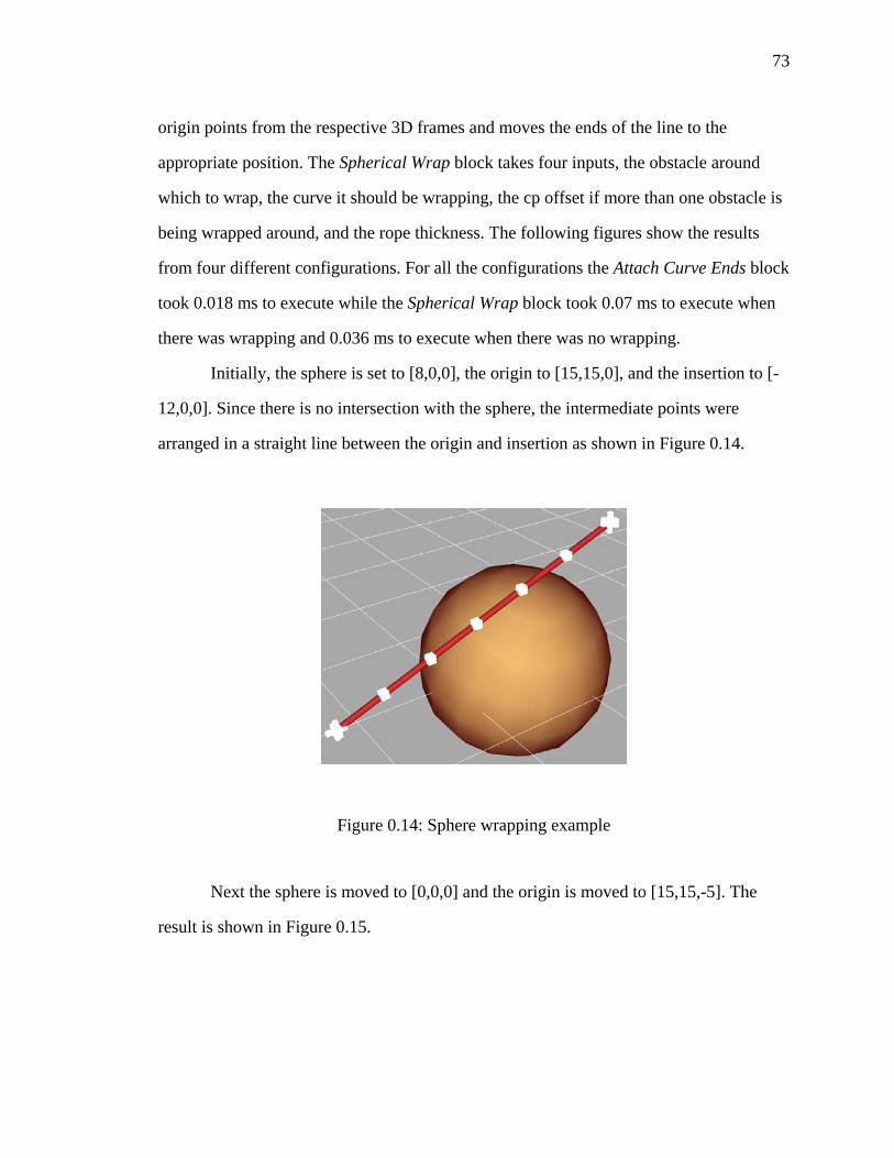
73

origin points from the respective 3D frames and moves the ends of the line to the

appropriate position. The Spherical Wrap block takes four inputs, the obstacle around

which to wrap, the curve it should be wrapping, the cp offset if more than one obstacle is

being wrapped around, and the rope thickness. The following figures show the results

from four different configurations. For all the configurations the Attach Curve Ends block

took 0.018 ms to execute while the Spherical Wrap block took 0.07 ms to execute when

there was wrapping and 0.036 ms to execute when there was no wrapping.

Initially, the sphere is set to [8,0,0], the origin to [15,15,0], and the insertion to [-

12,0,0]. Since there is no intersection with the sphere, the intermediate points were

arranged in a straight line between the origin and insertion as shown in Figure 0.14.

Figure 0.14: Sphere wrapping example

Next the sphere is moved to [0,0,0] and the origin is moved to [15,15,-5]. The

result is shown in Figure 0.15.

74

Figure 0.15: Sphere wrapping example

Then the origin is moved to [15,0,0] and the insertion is moved to[-12, 0.5, 0],

resulting in Figure 0.16.

Figure 0.16: Sphere wrapping example

Finally, the insertion is pushed to [-12, 0.5, -0.75], which result in Figure 0.17

75

Figure 0.17: Sphere wrapping example

Cylindrical Wrapping

The simulation for this example is comprised of a curve called curveToWrap with

7 control points, a cylinder called BlueCyl with a radius of 10 and a length of 25, and two

3D frames called insertion and origin, which represent the origin and insertion positions.

The logic of the simulation is shown in Figure 0.18, where the block Attach Curve Ends

holds the code that places the ends of the curve at the origin and insertion positions and

the block Cylinder Wrap holds the code which performs the cylindrical wrapping

algorithm described in the previous section.

Figure 0.18: Logic for cylinder wrapping example

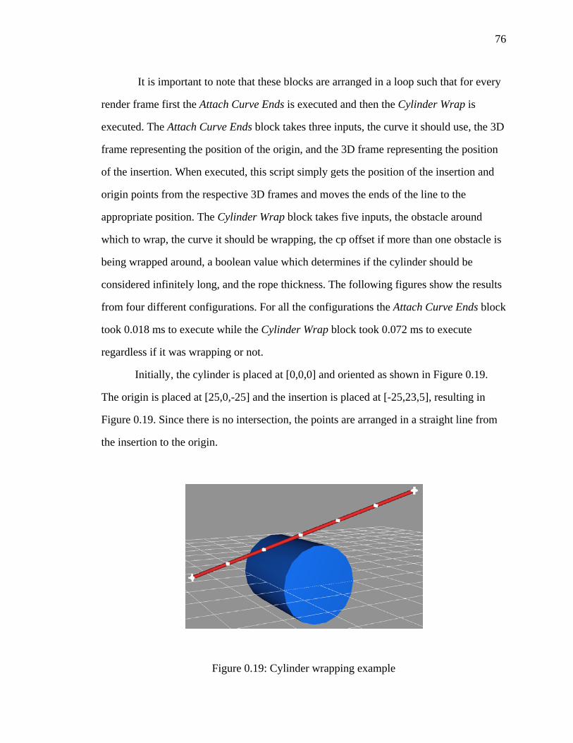
76

It is important to note that these blocks are arranged in a loop such that for every

render frame first the Attach Curve Ends is executed and then the Cylinder Wrap is

executed. The Attach Curve Ends block takes three inputs, the curve it should use, the 3D

frame representing the position of the origin, and the 3D frame representing the position

of the insertion. When executed, this script simply gets the position of the insertion and

origin points from the respective 3D frames and moves the ends of the line to the

appropriate position. The Cylinder Wrap block takes five inputs, the obstacle around

which to wrap, the curve it should be wrapping, the cp offset if more than one obstacle is

being wrapped around, a boolean value which determines if the cylinder should be

considered infinitely long, and the rope thickness. The following figures show the results

from four different configurations. For all the configurations the Attach Curve Ends block

took 0.018 ms to execute while the Cylinder Wrap block took 0.072 ms to execute

regardless if it was wrapping or not.

Initially, the cylinder is placed at [0,0,0] and oriented as shown in Figure 0.19.

The origin is placed at [25,0,-25] and the insertion is placed at [-25,23,5], resulting in

Figure 0.19. Since there is no intersection, the points are arranged in a straight line from

the insertion to the origin.

Figure 0.19: Cylinder wrapping example

77

Next, the insertion was moved to down to [-25,0,5], as shown in Figure 0.20.

Figure 0.20: Cylinder wrapping example

Then, the cylinder is moved up to [0,30,0], resulting in Figure 0.21.

Figure 0.21: Cylinder wrapping example

Finally, the cylinder is twisted about its z axis as shown in Figure 0.22.

78

Figure 0.22: Cylinder wrapping example

Multiple Obstacle Wrapping

The simulation for this example is comprised of a curve called curveToWrap with

17 control points, a cylinder called BlueCyl with a radius of 5 and a length of 25, another

cylinder called GreenCyl with a radius of 8 and a length of 18, a sphere called RedSphere

with a radius of 8, and two 3D frames called insertion and origin, which represent the

origin and insertion positions (Figure 0.23).

Figure 0.23: Setup for multiple obstacle wrapping example

79

The logic of the simulation is shown in Figure 0.24, where the block Attach Curve

Ends holds the code that places the ends of the curve at the origin and insertion positions,

the blocks Cylinder Wrap holds the code that performs the cylindrical wrapping

algorithm described in the previous section, and the block Spherical Wrap holds the code

which performs the spherical wrapping algorithm described in the previous section. It is

important to note that these blocks are arranged in a loop such that for every render frame

first the Attach Curve Ends is executed and then the first Cylinder Wrap is executed,

followed by the Spherical Wrap, and finally the second Cylinder Wrap.

Figure 0.24: Logic for multiple obstacle wrapping

The Attach Curve Ends block takes three inputs, the curve it should use, the 3D

frame representing the position of the origin, and the 3D frame representing the position

of the insertion. When executed, this script simply gets the position of the insertion and

origin points from the respective 3D frames and moves the ends of the line to the

appropriate position. The Cylinder Wrap block takes five inputs, the obstacle around

which to wrap, the curve it should be wrapping, the cp offset if more than one obstacle is

being wrapped around, a boolean value which determines if the cylinder should be

considered infinitely long, and the rope thickness. Note that the first block has a cp offset

of 0, the second block has a cp offset of 5 and the last block has a cp offset of 10. It is

important that the cp offset and the order in which the obstacles are encountered (from

the origin) correlate. For example, since the blue cylinder is encountered first its cp offset

80

should be zero. Figure 0.25 and Figure 0.26 show the results of one configuration. Total

execution time for all four blocks was 0.225 ms with the last Cylinder Wrap taking the

most time at 0.098 ms.

Figure 0.25: Multiple object wrapping example

Figure 0.26: Multiple object wrapping example

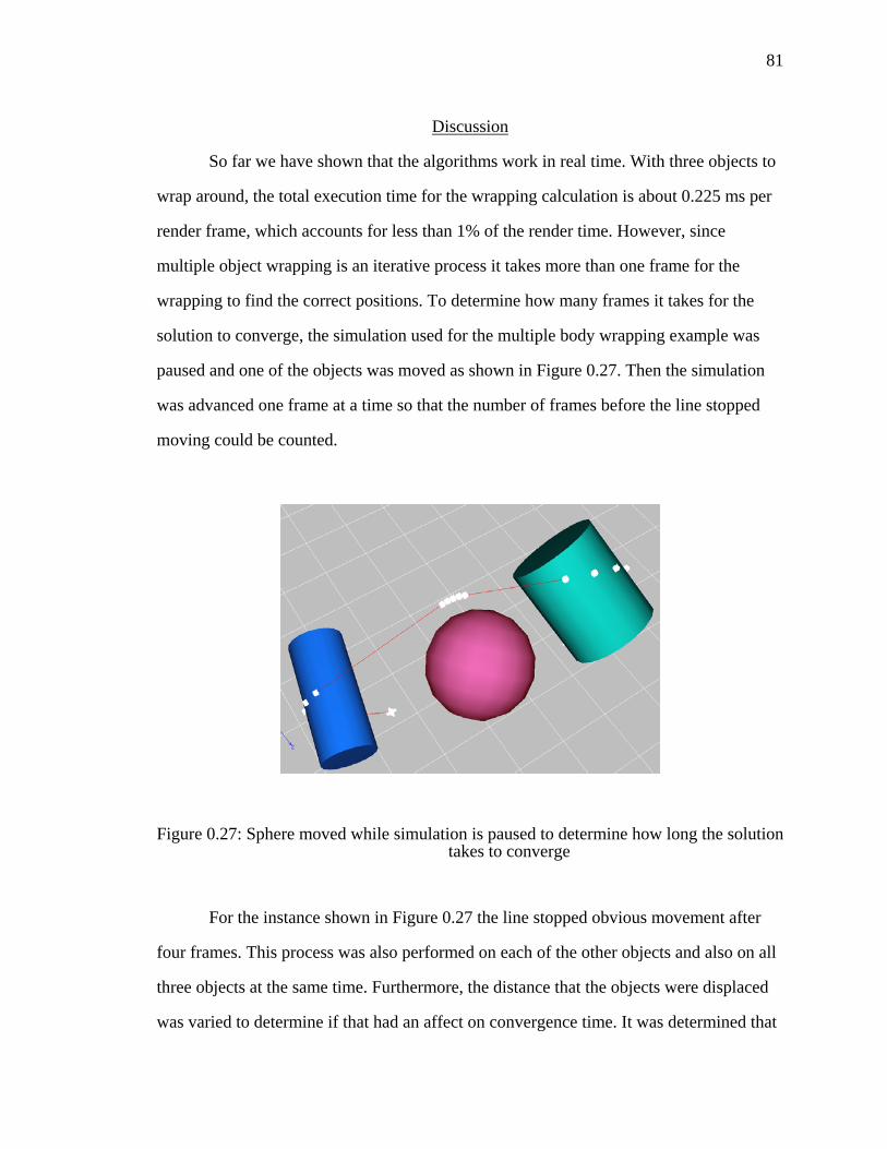
81

Discussion

So far we have shown that the algorithms work in real time. With three objects to

wrap around, the total execution time for the wrapping calculation is about 0.225 ms per

render frame, which accounts for less than 1% of the render time. However, since

multiple object wrapping is an iterative process it takes more than one frame for the

wrapping to find the correct positions. To determine how many frames it takes for the

solution to converge, the simulation used for the multiple body wrapping example was

paused and one of the objects was moved as shown in Figure 0.27. Then the simulation

was advanced one frame at a time so that the number of frames before the line stopped

moving could be counted.

Figure 0.27: Sphere moved while simulation is paused to determine how long the solution takes to converge

For the instance shown in Figure 0.27 the line stopped obvious movement after

four frames. This process was also performed on each of the other objects and also on all

three objects at the same time. Furthermore, the distance that the objects were displaced

was varied to determine if that had an affect on convergence time. It was determined that

82

distance does not significantly change the time to convergence but the number of objects

moved does. The longest convergence time encountered was when all three objects were

moved at the same time. 8 frames were counted before the line stopped obvious

movement. If the simulation is running real time (~30 fps) this translates into about 0.25

seconds. It should also be noted that in all cases, the first frame displayed the most drastic

change in positions.

During testing of the wrapping algorithms, a situation was discovered that caused

the wrapping to fail. This occurred when either an obstacle or one of the end points is

moved such that either the origin or the insertion moves within an obstacle. Since it is

impossible for any line originating from within a sphere or cylinder to be tangent to the

surface, the wrapping algorithm fails. This can be avoided by careful placement of the

obstacles.

Conclusions

It has been shown that a real time algorithm for wrapping about multiple known

objects is feasible. This chapter presented algorithms for wrapping around a sphere and a

cylinder and also detailed how to arrange these algorithms so that multiple objects could

be used. These algorithms will be useful for estimating a muscles centroid line or

multiple action lines (for muscles with wide attachment points) for any joint

configuration and in real time.

83

REAL TIME INTERACTION

Introduction

One way that our model is different from other models is that it is specifically

being designed to run real time. This implies that the model must respond to user input

instantly. For example, the user must have the ability to rotate the shoulder to arbitrary

orientation. During this movement, the action line for all the muscles should appear to

move as if they are really attached to the bones and wrapping over underlying objects.

Furthermore, the activation level of all the muscle should be constantly changing to

maintain the desired torques as the orientation changes. In this chapter we will discuss the

software in which the model was developed, the process used for enabling real time

interaction, and the graphical interface that will be used to relay information to the user.

Software

The group that is leading the way in real time interactivity is the video gaming

industry. In reality, the model we are developing will have interactivity like a video game

but also a scientific core dictating the output. Therefore an obvious place to look for

interactive 3D software is towards video game rendering engines and development

software. This software must have the following capabilities:

• Ability to import available 3D geometric models of the musculoskeletal

system

• Ability to render the objects in real time such that the objects can be

rotated and moved

• Ability to create a hierarchal structure of the bones and the attachment

points of the muscles

• Ability to create joints between the bone and limit the degrees of freedom

and range of these joints

• Ability to allow the user to interactively articulate the joints

84

• Ability to create lines representing the action lines of muscles which can

be changed as the arm is moved

• Enough programming structure to develop and deploy the wrapping

algorithms presented in chapter 5

• Ability to communicate with other software, which will handle the

optimization and the user interaction

After careful consideration Virtools™ was selected as the development software.

Not only did this fulfill the above requirements, it is also the software that the Virtual

Soldier Research lab is using to develop Santos™, which is where this model will

eventually be used. Virtools™ is a development tool that was initially created as

prototyping software for game developers. It allows simple graphical programming to

quickly develop interactive real time simulations. Furthermore, it also allows in depth

programming through either a SDK or a scripting language to develop more complicated

simulations.

The software selected for creating the simulation is very good for quickly creating

interactive real time simulation. However, it is somewhat onerous when it comes to

developing 2D user interfaces such as graphs, buttons, and information panels. Because

of this it was decided to create the interface window outside of Virtools™ in Microsoft

Visual Basic 6.0®, which is especially suited for creating graphic user interfaces. This

interface will display feedback graphs of various muscle data, allowing the user to change

the PSCA of the muscles and joint torques.

The last piece of software employed is a specialized program designed

specifically for solving optimization problems. This software will be used to solve the

optimization problem described in chapter 6. The program selected is called SNOPT and

is commercially available. SNOPT is used to minimize linear or nonlinear cost functions

with many variables and constraints. To find the minimum it uses a sequential quadratic

85

programming algorithm that obtains a search direction from a series of quadratic

programming sub problems. This results in a quick calculation of a local minimum.

Figure 0.1: Interaction between programs

These three programs will work together as shown in Figure 0.1 above. The user

will interact with both Virtools™ and Visual Basic®. Virtools™ will take care of

displaying the 3D model while communicating the moment arms of all the muscles to

Visual Basic®, which passes them on to SNOPT along with the desired torques and Fmax

for each muscle. SNOPT will return the predicted activation level of each muscle to

Visual Basic® which will take care of graphing all the appropriate data. Note that the

data being passed to SNOPT is based on the optimization formulation presented in

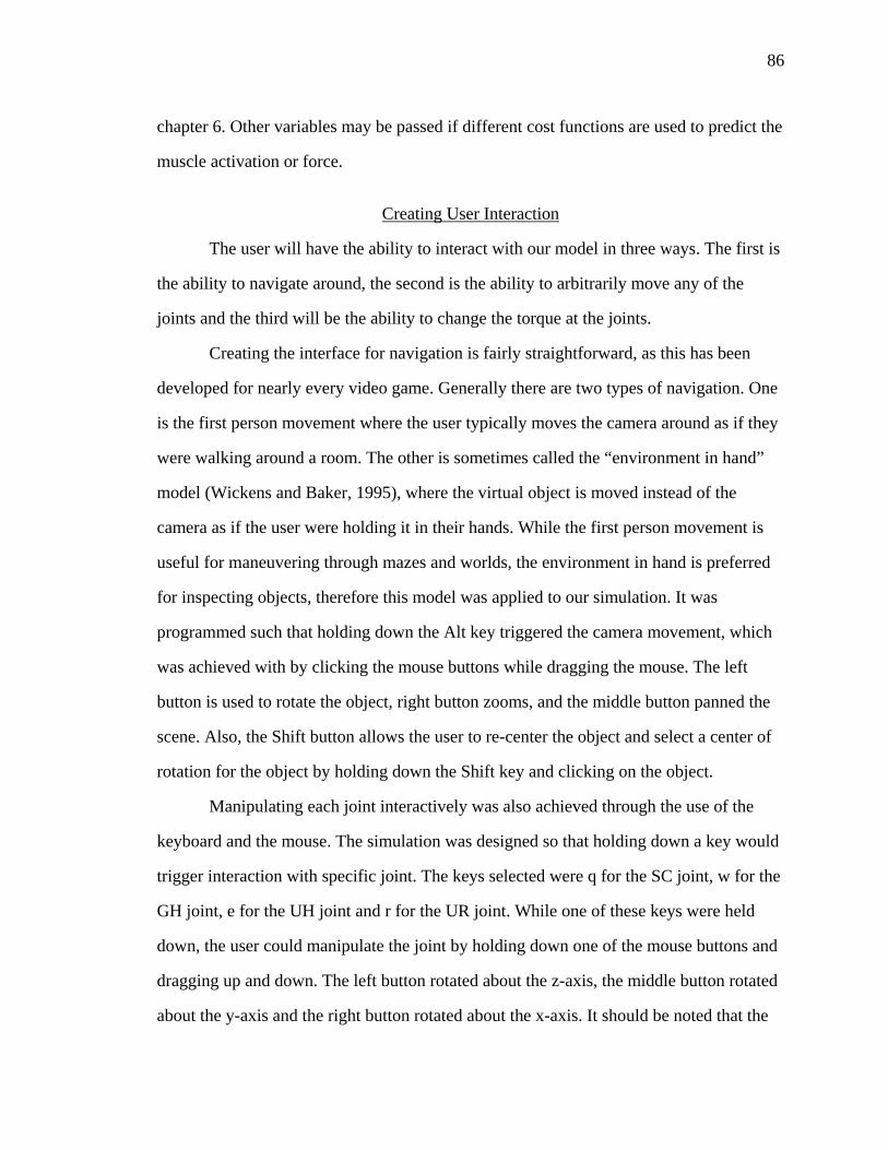
86

chapter 6. Other variables may be passed if different cost functions are used to predict the

muscle activation or force.

Creating User Interaction

The user will have the ability to interact with our model in three ways. The first is

the ability to navigate around, the second is the ability to arbitrarily move any of the

joints and the third will be the ability to change the torque at the joints.

Creating the interface for navigation is fairly straightforward, as this has been

developed for nearly every video game. Generally there are two types of navigation. One

is the first person movement where the user typically moves the camera around as if they

were walking around a room. The other is sometimes called the “environment in hand”

model (Wickens and Baker, 1995), where the virtual object is moved instead of the

camera as if the user were holding it in their hands. While the first person movement is

useful for maneuvering through mazes and worlds, the environment in hand is preferred

for inspecting objects, therefore this model was applied to our simulation. It was

programmed such that holding down the Alt key triggered the camera movement, which

was achieved with by clicking the mouse buttons while dragging the mouse. The left

button is used to rotate the object, right button zooms, and the middle button panned the

scene. Also, the Shift button allows the user to re-center the object and select a center of

rotation for the object by holding down the Shift key and clicking on the object.

Manipulating each joint interactively was also achieved through the use of the

keyboard and the mouse. The simulation was designed so that holding down a key would

trigger interaction with specific joint. The keys selected were q for the SC joint, w for the

GH joint, e for the UH joint and r for the UR joint. While one of these keys were held

down, the user could manipulate the joint by holding down one of the mouse buttons and

dragging up and down. The left button rotated about the z-axis, the middle button rotated

about the y-axis and the right button rotated about the x-axis. It should be noted that the

87

joint with only 1DOF could only be manipulated with the left mouse button. It should

also be noted that there is no interaction programmed for the AC joint. This is because

the AC joint moves in rhythm with the GH and the SC joints.

The interaction for changing the torques were incorporated into the Visual Basic

interface as sliders (Figure 0.2). Through this interface the user has the ability to specify

the torque about the x, y, and z axis for all five joints.

Figure 0.2: Joint torque user interface. For the joints with more than 1DOF the sliders are arranged such that the top slider is torque about x, middle slider is torque

about y and the bottom slider is torque about z.

Data Feedback

This model incorporates 35 action lines, each of which affects at least one joint

with at least one degree of freedom. Some muscles, such as the pectorals major originate

on the torso and insert on the humerus. Because of this, it affects three spherical joints

(the GH, AC, and SC). What this boils down to is that this model will generate a whole

lot of data that needs to be conveyed to the user in a logical manner. It was decided to

display three main pieces of data. First will be the moment arms that each muscle creates

88

about the joint or joints that it crosses for any limb configuration. Second will be the max

torque that each muscle can apply to each joint or joints that it crosses for any limb

configuration. Lastly it will display the predicted activation level of all the muscles for a

given set of joint torques and arm configuration. All this data will be displayed as bar

graphs in a qualitative manner.

Moment Arm Display

The moment arms are calculated within Virtools™ and passed to Visual Basic.

They have to be calculated in Virtools™ because they are derived from the geometry and

the action lines of each muscle. The moment arms were calculated with the following

equation where r is the vector pointing from the joint to where the action line inserts and

F is the unit vector pointing along the action line at the point of insertion.

Frma ˆ×= (6.1)

Figure 0.3: Moment Arms of muscles crossing the sterno-clavicular joint

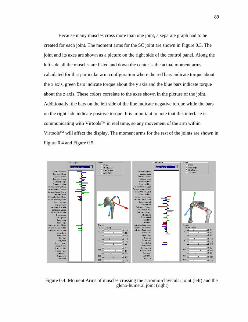
89

Because many muscles cross more than one joint, a separate graph had to be

created for each joint. The moment arms for the SC joint are shown in Figure 0.3. The

joint and its axes are shown as a picture on the right side of the control panel. Along the

left side all the muscles are listed and down the center is the actual moment arms

calculated for that particular arm configuration where the red bars indicate torque about

the x axis, green bars indicate torque about the y axis and the blue bars indicate torque

about the z axis. These colors correlate to the axes shown in the picture of the joint.

Additionally, the bars on the left side of the line indicate negative torque while the bars

on the right side indicate positive torque. It is important to note that this interface is

communicating with Virtools™ in real time, so any movement of the arm within

Virtools™ will affect the display. The moment arms for the rest of the joints are shown in

Figure 0.4 and Figure 0.5.

Figure 0.4: Moment Arms of muscles crossing the acromio-clavicular joint (left) and the gleno-humeral joint (right)

90

Figure 0.5: Moment arms of muscles crossing the ulno-humeral joint (left) and the ulno-radial joint (right)

Max Torque Display

Max torque contributed by each muscle is calculated with the equation 6.2 where

ma is the moment arm calculated with equation 6.1 and Fmax is the maximum force that

the muscle can generate, which can be calculated by the physical cross sectional area

(PCSA) and the maximum muscle stress, as shown in equation 6.3. The PCSA for each

muscle was found in literature (Maurel and Thalmann, 1999) and 600 kPa was used for

the maximum muscle stress (Berme et al., 1987). As with the moment arm data, this is

displayed as qualitative bar graphs for each joint. The resulting display is shown in

Figure 0.6, Figure 0.7, and Figure 0.8.

( ) maFFrFFrT maxmaxmaxmaxˆ =×=×= (6.2)

maxmax *σPCSAF = (6.3)

91

Figure 0.6: Max torque of muscles crossing the sterno-clavicular joint

Figure 0.7: Max torque of muscles crossing the acromio-clavicular joint (left) and the gleno-humeral joint (right)

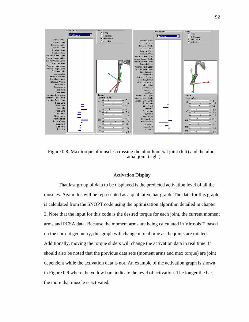
92

Figure 0.8: Max torque of muscles crossing the ulno-humeral joint (left) and the ulno-radial joint (right)

Activation Display

That last group of data to be displayed is the predicted activation level of all the

muscles. Again this will be represented as a qualitative bar graph. The data for this graph

is calculated from the SNOPT code using the optimization algorithm detailed in chapter

3. Note that the input for this code is the desired torque for each joint, the current moment

arms and PCSA data. Because the moment arms are being calculated in Virtools™ based

on the current geometry, this graph will change in real time as the joints are rotated.

Additionally, moving the torque sliders will change the activation data in real time. It

should also be noted that the previous data sets (moment arms and max torque) are joint

dependent while the activation data is not. An example of the activation graph is shown

in Figure 0.9 where the yellow bars indicate the level of activation. The longer the bar,

the more that muscle is activated.

93

Figure 0.9: Predicted activation levels

Conclusion

In this chapter we have presented the software used for development and the real

time interfaces for both user input and data feedback. We have presented all the pieces of

the research used to create our interactive arm model. In the next chapter we will present

various examples and discuss the results.

94

RESULTS AND DISCUSSION

Introduction

In this chapter we will start out by examining the lower arm, which includes the

elbow (UH), the hand pronation joint (UR) and the associated muscles crossing them.

Then we will examine the pectoral girdle, which includes the three shoulder joints (SC,

AC, and GH) and the associated muscles. Finally we will present the system as a whole.

For each region we will examine the computed moment arms, max torque, and predicted

activation levels for the associated muscles and discuss the data. In all the examples, the

moment arms were calculated from equation 6.1 in chapter 6, max torque was calculated

from equation 6.2 in chapter 6 and the predicted activation levels were calculation from

the optimization algorithm presented in chapter 3. The PCSA data and max muscle stress

values used are shown in Figure 0.1 (Maurel, 1999). For these examples, these values

were held constant. At the end of the chapter we will present some preliminary

comparisons of our model to previous models.

Figure 0.1: Max muscle stress (kPa) and PCSA (cm2) data used in the examples

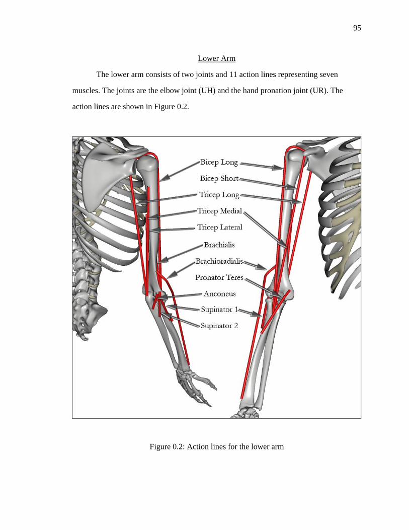
95

Lower Arm

The lower arm consists of two joints and 11 action lines representing seven

muscles. The joints are the elbow joint (UH) and the hand pronation joint (UR). The

action lines are shown in Figure 0.2.

Figure 0.2: Action lines for the lower arm

96

First we examine how the action line wrapping algorithm presented in chapter 5 is

working. Figure 0.3 shows the lower arm in three configurations. Note how the six action

lines wrap over the distal end of the humerus and the Supinator 1 action line wraps about

the radius as the hand is pronated. It is important to emphasize that this wrapping is

occurring in real time as the joints are interactively being rotated.

Figure 0.3: Action lines wrapping around the elbow. From left to right: elbow fully extended with hand supinated, elbow halfway flexed with hand supinated,

elbow fully flexed with hand pronated

Next we will move position the lower arm in various positions and look at the

moment arms, max torque and predicted activation levels for the muscles. Figure 0.4

displays the first configuration and resulting moment arms and max torque. In this

configuration the elbow if fully extended and the hand is neutral, which we define as

halfway between pronation and supination. The graphs in the figure display the moment

arms and max torque about each joint for each muscle. By observing the graphs for the

elbow joint (UH) one will note that all the action lines shown create torque about the UH

joint while only five create a moment about the UR joint. This is appropriate because

while all the action lines cross the elbow joint (i.e. they originate on a bone which is

proximal to the elbow and insert on a bone which is distal to the elbow) not all the

97

muscles cross the UR joint. Specifically, the muscles which insert on the radius cross

both the UR and UH joint while the muscles that insert on the ulna only cross the UH

joint.

Figure 0.4: Example 1; Hand is neutral and the elbow if fully extended. The charts show the moment arms and max torque about each joint for all 11 action lines of the

lower arm

98

By looking at the sign of the moment arm we can also determine what action that

muscle will have on the respective joint. All the action lines with positive moment arms

on the UH joint are used for flexion while the action lines with negative moment arms are

used for extension. As expected, the triceps, supinator, and anconeus are all used for

extension while the biceps, brachialis, brachioradialis, and pronator teres are used for

flexion. The three triceps action lines have the largest moment arm for extending the arm

while the brachioradialis has the largest moment arm for flexion. However, the maximum

torque that these muscles can apply is also dependent on the size of the muscle. The main

extension muscles are still the triceps but there are two major flexion muscles, the

brachioradialis and the brachialis. Even though the brachialis has a short moment arm, its

size lets it create almost as much torque as the brachioradialis.

At the UR joint, a positive moment arm indicates the muscle is used for

supination of the hand while a negative moment arm is used for pronation. Therefore it

can be observed that all the muscles crossing this joint are used for supination except for

the pronator teres and the muscle that can contribute the most torque towards supination

is the brachioradialis. It should be noted that these graphs should only be used for

qualitative comparison to the other action lines in the same graph. The size of the bars

displaying torque about the UR joint cannot be compared to the size of the bars

displaying torque about the UH joint.

Figure 0.5: Predicted muscle activation for various torques

99

Next we will look at the predicted activation levels of all the muscles to achieve a

desired torque as shown in Figure 0.5. Note that the arm is still in the configuration as

shown in Figure 0.4. Initially, the slider for the elbow torque was increased until no

feasible solution was found by the optimization code, then the slider was stepped back so

a solution was found at the very edge of the feasible space. This resulted in a flexion

torque about the elbow of 8 Nm as shown in the first graph of Figure 0.5. It is interesting

to note that while the optimization code is telling us this the max torque we can generate

about the elbow, only three muscles are active; the brachialis, brachioradialis, and

pronator teres. This is because we have constrained the torque about the UR joint to be

zero. The brachialis, which creates no torque about the UR, (refer to Figure 0.4) is fully

activated because it is the only muscle that creates a positive torque about UH without

affecting UR. The brachioradialis is also slightly activated to help create torque about the

elbow but it also creates positive torque about the UR joint since it inserts on the radius.

In order to maintain zero torque about the UR joint, the pronator teres, which is the only

muscle that is available to create negative torque about the UR, is activated to counter

positive torque created by the brachioradialis. The step size on the slider used to select

how much torque is desired about the elbow is 0.1 Nm. Allowing a finer step size on the

elbow torque slider may reveal that a little more torque could be generated because the

pronator teres is not fully activated, thus the brachioradialis could be activated a little

more. Finally, it can also be observed that the two flexion muscles with the largest

moment arms were the muscles that were activated to generate the positive torque.

In the second graph of Figure 0.5, the torque about the UR joint is moved up to 2

Nm while the torque about UH is left at 8 Nm. Note that the brachioradialis is now fully

activated, the brachialis’ activation has been significantly reduced, and the pronator teres

is no longer activated. Furthermore, both the biceps and a supinator muscle are now

activated. The brachioradialis is fully activated because it has the ability to create the

largest positive torque about both the joints, thus contributing to both of the desired

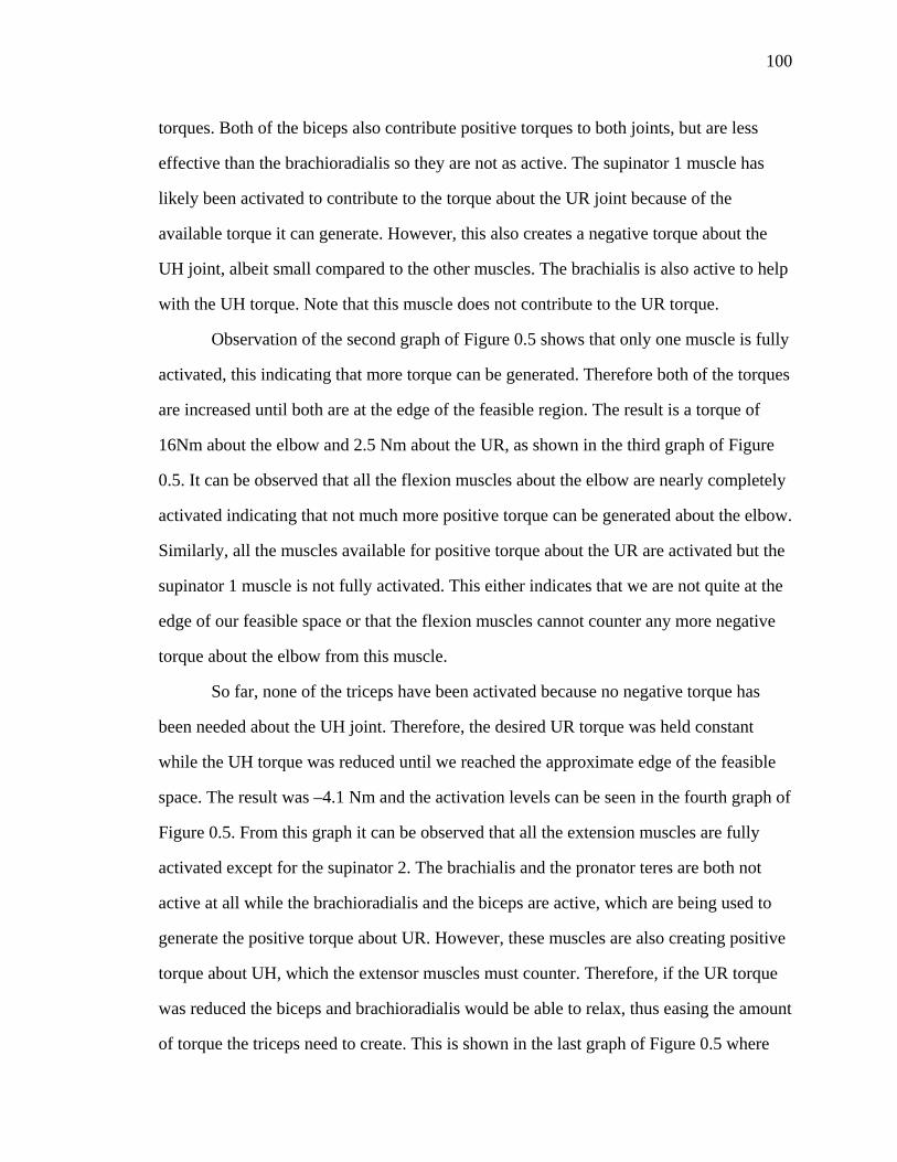
100

torques. Both of the biceps also contribute positive torques to both joints, but are less

effective than the brachioradialis so they are not as active. The supinator 1 muscle has

likely been activated to contribute to the torque about the UR joint because of the

available torque it can generate. However, this also creates a negative torque about the

UH joint, albeit small compared to the other muscles. The brachialis is also active to help

with the UH torque. Note that this muscle does not contribute to the UR torque.

Observation of the second graph of Figure 0.5 shows that only one muscle is fully

activated, this indicating that more torque can be generated. Therefore both of the torques

are increased until both are at the edge of the feasible region. The result is a torque of

16Nm about the elbow and 2.5 Nm about the UR, as shown in the third graph of Figure

0.5. It can be observed that all the flexion muscles about the elbow are nearly completely

activated indicating that not much more positive torque can be generated about the elbow.

Similarly, all the muscles available for positive torque about the UR are activated but the

supinator 1 muscle is not fully activated. This either indicates that we are not quite at the

edge of our feasible space or that the flexion muscles cannot counter any more negative

torque about the elbow from this muscle.

So far, none of the triceps have been activated because no negative torque has

been needed about the UH joint. Therefore, the desired UR torque was held constant

while the UH torque was reduced until we reached the approximate edge of the feasible

space. The result was –4.1 Nm and the activation levels can be seen in the fourth graph of

Figure 0.5. From this graph it can be observed that all the extension muscles are fully

activated except for the supinator 2. The brachialis and the pronator teres are both not

active at all while the brachioradialis and the biceps are active, which are being used to

generate the positive torque about UR. However, these muscles are also creating positive

torque about UH, which the extensor muscles must counter. Therefore, if the UR torque

was reduced the biceps and brachioradialis would be able to relax, thus easing the amount

of torque the triceps need to create. This is shown in the last graph of Figure 0.5 where

101

the desired UR torque is set to zero. From the graph it can be observed that none of the

extensor muscles are fully activated, implying that more negative torque can easily be

generated at the elbow. It can also be noted that the only extensor muscle that is not

activated at all is the supinator 1 muscle, which is the only extensor muscle that also

creates torque about the UR joint.

Figure 0.6: Example 2; Hand is neutral and the elbow if fully flexed. The charts show the max torque about each joint for all 11 action lines of the lower arm

102

In the second example the hand is left neutral while the

elbow is fully flexed to 120° as shown in Figure 0.6. This

time only the max torque is displayed for each muscle.

When compared to the max torques of Figure 0.4 one will

observe that a number of muscles used for flexion and

extension is the same. Similarly, the number of pronating

and supinating muscles about the UR joint are also the

same. When considering the amount of available torque

about the UR joint, it should be noted that the amount of

available negative torque is less while the amount of

available positive torque is considerably greater. The max

torque of the brachialis is about the same but the max

torque of the brachioradialis has nearly doubles while the

max torque of both biceps have nearly tripled. All the max

torques of the extensor muscles have shrunk somewhat

indicating that the arm has less capability for creating

negative torque in this position. There is not much change

noted in the max torques of the muscles crossing the UR

joint. Since the PCSA is considered constant, the difference

in available torque between the two arm positions is due to

a change in the moment arms.

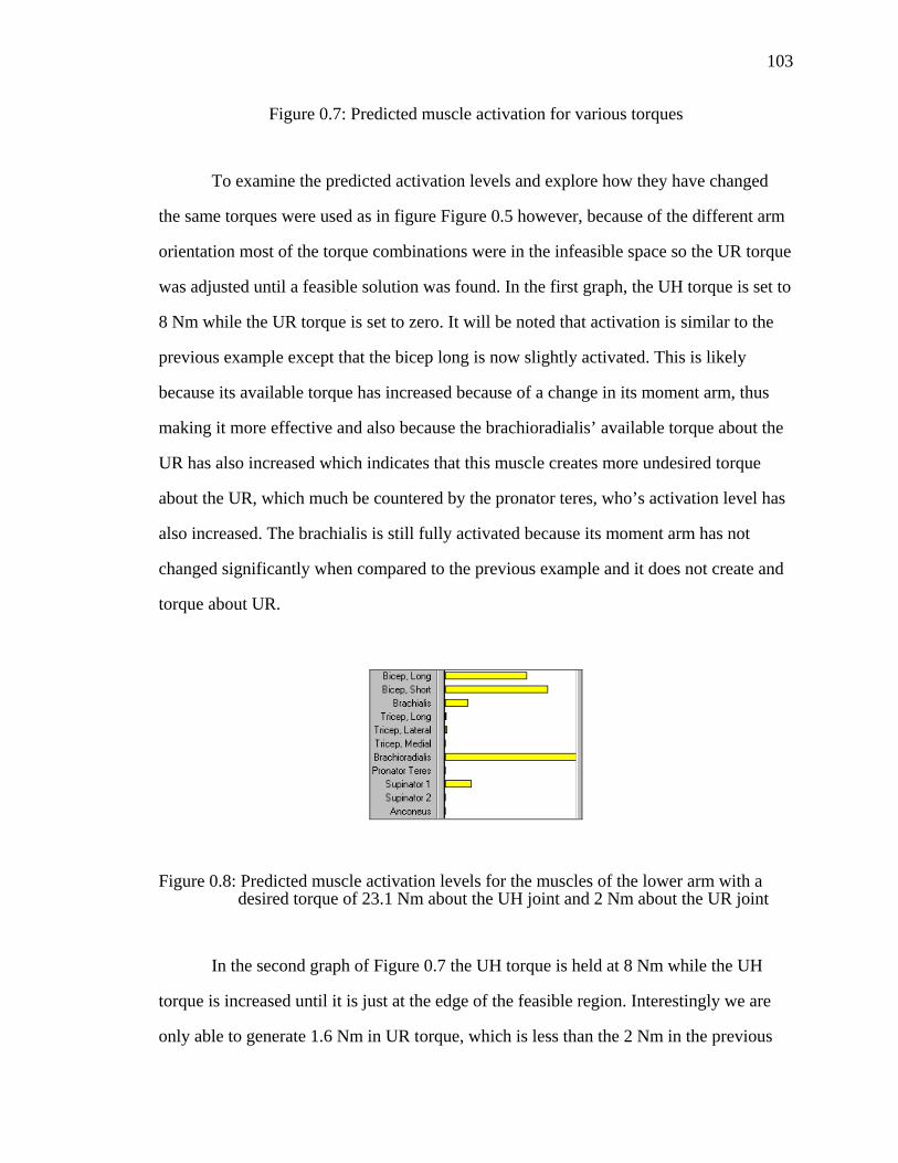
103

Figure 0.7: Predicted muscle activation for various torques

To examine the predicted activation levels and explore how they have changed

the same torques were used as in figure Figure 0.5 however, because of the different arm

orientation most of the torque combinations were in the infeasible space so the UR torque

was adjusted until a feasible solution was found. In the first graph, the UH torque is set to

8 Nm while the UR torque is set to zero. It will be noted that activation is similar to the

previous example except that the bicep long is now slightly activated. This is likely

because its available torque has increased because of a change in its moment arm, thus

making it more effective and also because the brachioradialis’ available torque about the

UR has also increased which indicates that this muscle creates more undesired torque

about the UR, which much be countered by the pronator teres, who’s activation level has

also increased. The brachialis is still fully activated because its moment arm has not

changed significantly when compared to the previous example and it does not create and

torque about UR.

Figure 0.8: Predicted muscle activation levels for the muscles of the lower arm with a desired torque of 23.1 Nm about the UH joint and 2 Nm about the UR joint

In the second graph of Figure 0.7 the UH torque is held at 8 Nm while the UH

torque is increased until it is just at the edge of the feasible region. Interestingly we are

only able to generate 1.6 Nm in UR torque, which is less than the 2 Nm in the previous

104

example, even though the available torques about the UR joint have not changed

significantly. A major difference noted between this and the previous example is the near

full activation of all the extensor muscles indicating that excessive positive torque is

being created about the UH joint in order to achieve the desired UR torque. Further

inspection will reveal that the muscle with the smallest available torque about the elbow

(with exception to the pronator teres, which is not being used because it also creates

negative torque about the UR joint) is the only flexion muscle that is fully activated. In

fact the only other flexion muscle activated is the brachioradialis, which also has the

largest amount of available torque about the UR joint. So, what has happened is that the

moment arms used to create the UR torque have not changed significantly but the

moment arms about the UH joint have and since positive UR torque is primarily

generated by the biceps and the brachioradialis the activation needed to create the UR

torque is creating excessive positive torque about the UH. Therefore, if more torque is

allowed about the UH then the extensor muscles will be able to relax and the graph will

begin to look more like the previous example as can be seen in Figure 0.8 where the UH

torque is raised to 23.1 Nm and the UR joint torque is raised to 2 Nm.

Next the UH joint torque is raised to 16 Nm and the UR joint torque is raised to

2.4 Nm in order to compare with the previous example. Note that in the previous

example, the UR joint torque was set to 2.5 Nm, however in this configuration this was

just outside of the feasible space so the UR joint torque was set to 2.4, which was within

the feasible space. The result is displayed as the third graph in Figure 0.7. Again, all the

extensor muscle are active while only two of the flexion muscles are being used

indicating that excessive torque is being generated about the UH joint. As with the

previous scenario, the significant increase in the moment arms of the biceps and

brachioradialis about the UH joint while having insignificant increases in the moment

arms about the UR joint have reduced the feasible space. Allowing more torque about the

elbow expands the feasible space and results in an activation pattern similar to the

105

previous example, as is shown in Figure 0.9 where the UH joint torque was raised to 38.7

Nm and the UR joint torque was raised to 2.5 Nm.

Figure 0.9: Predicted muscle activation levels for the muscles of the lower arm with a desired torque of 36.7 Nm about the UH joint and 2.5 Nm about the UR joint

The final graph in Figure 0.7 shows the result of setting the UH torque to –4.1 and

the UR torque to 0.2. Because the available torque of the extension muscles has

decreased so has the feasible space. This can be observed in the graph by noting that

nearly all the extensor muscles are fully activated, including the supinator 1 muscle,

which also creates positive torque about the UR axis. Therefore, if less UR torque is

desired there are two options. One is to create positive UR torque with the pronator teres

in order to counter the torque being generated by the supinator muscle. However, this

would cause positive torque about the UH joint as well, which would have to be

countered with the triceps lateral. The other option is to relax the supinator 1 so as to

reduce the amount UR torque it is creating. However this will also reduce the amount of

negative torque it is contributing to the UH joint. This reduction will have to be balanced

with an increase of activation in the tricep lateral. Either solution will require the triceps

lateral to have an increase in activation and from the graph is can be observed that it is

already nearly fully activated. Conversely, if more torque was desired about the UR there

are again two solutions. One is to allow the supinator 1 muscle to become more active,

thus increasing the torque about the UR joint and also contributing more negative torque

106

to the UH joint. This will have to be balanced by a reduction in the activation of the other

extension muscles. However, one will note that this solution is maximized when the

supinator 1 muscle is fully activated, which it nearly is already. The other solution is to

create more torque about the UR with one of the bicep muscles. However, any activation

of the bicep will cause positive torque about the UH, which will have to be balanced by

the extensor muscles who are already nearly fully activated.

In the previous two examples the elbow was flexed while the UR joint was left

fixed. In the next three examples, the elbow will be left fixed at about mid flexion and the

hand will be pronated then supinated to observe what changes that causes. The first of

these three examples is shown in Figure 0.10 where the hand is neutral. Displayed is the

max torque about each joint for each action line as well as the predicted activation level

for the muscles for two different torque configurations.

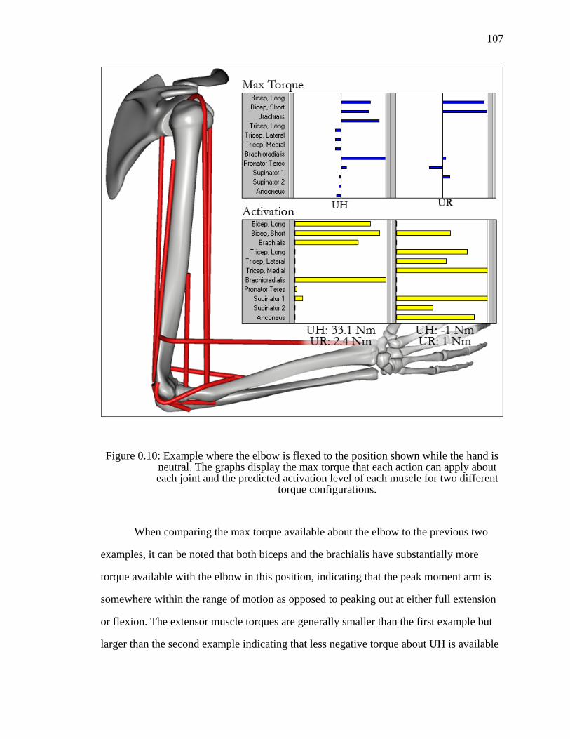
107

Figure 0.10: Example where the elbow is flexed to the position shown while the hand is neutral. The graphs display the max torque that each action can apply about each joint and the predicted activation level of each muscle for two different

torque configurations.

When comparing the max torque available about the elbow to the previous two

examples, it can be noted that both biceps and the brachialis have substantially more

torque available with the elbow in this position, indicating that the peak moment arm is

somewhere within the range of motion as opposed to peaking out at either full extension

or flexion. The extensor muscle torques are generally smaller than the first example but

larger than the second example indicating that less negative torque about UH is available

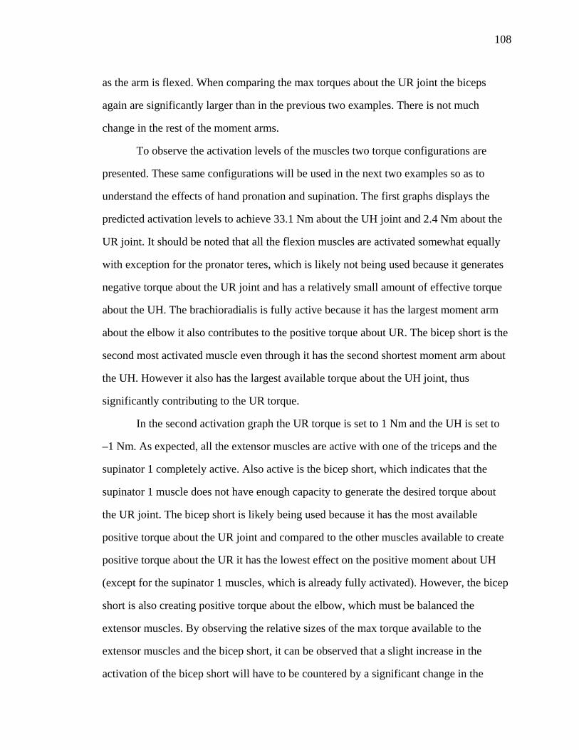
108

as the arm is flexed. When comparing the max torques about the UR joint the biceps

again are significantly larger than in the previous two examples. There is not much

change in the rest of the moment arms.

To observe the activation levels of the muscles two torque configurations are

presented. These same configurations will be used in the next two examples so as to

understand the effects of hand pronation and supination. The first graphs displays the

predicted activation levels to achieve 33.1 Nm about the UH joint and 2.4 Nm about the

UR joint. It should be noted that all the flexion muscles are activated somewhat equally

with exception for the pronator teres, which is likely not being used because it generates

negative torque about the UR joint and has a relatively small amount of effective torque

about the UH. The brachioradialis is fully active because it has the largest moment arm

about the elbow it also contributes to the positive torque about UR. The bicep short is the

second most activated muscle even through it has the second shortest moment arm about

the UH. However it also has the largest available torque about the UH joint, thus

significantly contributing to the UR torque.

In the second activation graph the UR torque is set to 1 Nm and the UH is set to

–1 Nm. As expected, all the extensor muscles are active with one of the triceps and the

supinator 1 completely active. Also active is the bicep short, which indicates that the

supinator 1 muscle does not have enough capacity to generate the desired torque about

the UR joint. The bicep short is likely being used because it has the most available

positive torque about the UR joint and compared to the other muscles available to create

positive torque about the UR it has the lowest effect on the positive moment about UH

(except for the supinator 1 muscles, which is already fully activated). However, the bicep

short is also creating positive torque about the elbow, which must be balanced the

extensor muscles. By observing the relative sizes of the max torque available to the

extensor muscles and the bicep short, it can be observed that a slight increase in the

activation of the bicep short will have to be countered by a significant change in the

109

extensor muscles. For example, consider if the bicep short were to increase its activation

by 0.1. For this to be countered by one of the tricep muscles, who’s available torque is

about five times smaller, it would have to increase it’s activation level by approximately

0.5. Therefore, it can be concluded that any slight increase in the amount of positive

torque about the UR is going to limit the amount of available negative torque about the

UH because the extensors will have to use more torque to counter the increase of the

positive torque being created about the UH.

In the next example, the elbow is held in the same position while the hand is

pronated as shown in Figure 0.11. When comparing the max torques of this example to

the previous example it is interesting to note that the torques about the UH show no

significant change while all the max torques except for the supinator 1 show significant

changes about the UR axes. The max torque of both the biceps have dropped

substantially while the brachioradialis has as increased dramatically. Also, the pronator

teres has changed signs, indicating that there are no muscles available to create and

pronation torque.

When comparing the activation levels of this example with the previous example

some slight differences can be observed. Since there was insignificant changes in the max

torques about the UH, the changes in activation can be attributed to the changes in the

moment arms about the UR joints. In the first activation graph of Figure 0.11 where the

UH and UR torques are set to 33.1 Nm and 2.4 Nm, respectively, the supinator 1 is no

longer active, the brachialis is now fully active, and the biceps activation have been

somewhat reduced. The reduction of the biceps and the supinator 1 indicate that the

brachioradialis is now able to create the majority of the UR torque needed, which is

reasonable considering the increase in its available torque. This is further emphasized by

the increased activation of the brachialis, which does not create any UR torque.

Furthermore it should be noted that the two muscles with the most available torque about

UH are the two muscles that are fully activated.

110

Figure 0.11: Example where the elbow is flexed to the postion shown while the hand is pronated. The graphs display the max torque that each action can apply about each joint and the predicted activation level of each muscle for two different

torque confuguratons.

Looking at the second activation graph in Figure 0.11 a more significant change

can be noted, particularly in the bicep short and the pronator teres. The bicep is no longer

active while the pronator teres is now full active. This is likely because pronator teres

now has the ability to create significant positive torque about the UR joint while creating

a smaller amount of positive torque about UH joint as compared to the bicep short

111

muscle. It should also be noted that none of the extensor muscles are fully activated,

indicating that there is capacity to create more negative torque about the UH joint.

Figure 0.12: Example where the elbow is flexed to the postion shown while the hand is spinated. The graphs display the max torque that each action can apply about each joint and the predicted activation level of each muscle for two different

torque confuguratons.

In the final example of the lower arm we again keep the elbow fixed but supinate

the hand as shown in Figure 0.12. By comparing the max torques about the joints with

Figure 0.10 and Figure 0.11 we see that there is still insignificant change in the max

112

torques about UH and significant changes in the max torques about the UR joint. The

biceps both have max torque values similar to when the hand is in its neutral position

(Figure 0.10) while the brachioradialis is now creating substantial pronation torque along

with the pronator teres and the supinator 1 has very little capacity for creating torque on

either joint.

In comparing the first activation graph we see that this graph is more similar to

when the hand is pronated than when the hand is neutral except the brachioradialis is less

active while the biceps activity has increased. This is likely because activating the

brachioradialis now creates substantial pronation torque, which must be balanced by the

biceps. It is interesting to note that nearly all the flexion muscles are fully activated with

exception of the pronator teres, which cannot contribute much to the UR torque and will

also create negative torque about the UR joint. This torque will have to be balanced but

the biceps are already fully activated which implies that this torque must be countered by

the supinator 1, whose available torque is fairly insignificant. Therefore it can be

ascertained that 33.1 Nm is nearing the limit of UH torque in this configuration while

requiring 2.4 Nm about the UR joint. If the required torque about the UR joint is reduced,

then both the brachioradialis and the pronator teres will be able to create more positive

torque about the UH joint because further activation of either of these muscles will create

more negative torque about the UR joint.

The second activation graph of Figure 0.12 show the predicted muscle activation

levels for a torque of –1 Nm about the UH and 1 Nm about the UR. The result is quite

similar to the predicted activation when the hand is in the neutral position (Figure 0.10)

except the bicep long is active instead of the bicep short and the supinator 1 activation

level has dropped while the anconeus has increased slightly. This could be because the

available torque from the supinator 1 has been reduced, thus making it less effective for

creating UR torque. Therefore its activity was reduced and the anconeus was activated to

make up for the negative torque about the UH that the supinator 1 previously created. It is

113

unclear why the bicep muscles have flipped activation. It is possible the bicep long

muscle is slightly more effective at creating UR torque than the bicep short but this

cannot be seen in the graph.

Pectoral Girdle

The pectoral girdle consists of three joints and 24 action lines representing 16

muscles. The joints are the sterno-calvicular (SC), the acromio-clavicualar (AC) and the

gleno-humeral (GH). The action lines are shown in Figure 0.13. Note that this figure does

not show two action lines which are the trapezius long extending from the ulna to the

scapula and the bicep long which extends from the radius to the scapula (refer to Figure

0.2).

Figure 0.13: Action lines of the pectoral girdle

After looking at Figure 0.13 one begins to understand just how complex the

pectoral girdle is. Not only does it have 24 action lines, it also has three spherical joints.

114

Furthermore, many of the action lines cross all three joints, thus having the possibility to

create torque about nine different axes. In the previous section, we were dealing with two

rotation axes so understanding the predicted activation levels was fairly simple. This will

not be the case for the shoulder muscles. In this section several examples will be

presented along with the corresponding data. To make analysis somewhat easier, only the

max torque about the SC and GH joint will be presented along with some activation

results.

Figure 0.14: Example of the pectoral girdle. Graphs display max torque about the SC and GH joint

115

The first example is displayed in Figure 0.14 where the graphs represent the

maximum available torque from each action line about the SC and GH joint. Just above

each graph is an image of the respective joint along with the axes of rotation where red is

the x axis, y is the green axis and blue is the z axis. The torques shown in the graphs are

also colored such that red indicates torque about the red (x axis), etc. Additionally, the

direction of the rotation is based on the right hand rule. Further descriptions of the joint

axes can be found in chapter 4.

Looking at the first graph we can start to get a feel for how movement or torque is

created about the clavicle. By observing the graph it can be noted that 15 action lines

cross the SC joint. As expected, all these action lines originate somewhere on the thorax

and insert on either the scapula or the humerus. Essentially, there are two movement

associated with the clavicle. Negative rotation about x-axis will cause a shrugging motion

at the shoulder while positive rotation about the z will push the shoulder backwards.

Rotations about the y-axis are minimal, therefore will not be discussed. Starting with the

shrugging of the shoulder, which is created by negative torque about the x, we can see

that four muscles can be used for this in this posture, the levator scapulae, upper

trapezius, the rhomboids, and the latissimus dorsi. While levator scapulae, upper

trapezius, and the rhomboids seem reasonable the latissimus dorsi doesn’t. After careful

inspection of the code the reason for this is still unclear and should be addressed in future

work. Positive torque about the x-axis is generated with the lower trapezius, the serratus

anterior and the pectoralis major and minor, all of which seem reasonable. Negative

torque about the z-axis is created with the serratus anterior and the pectoralis major and

minor muscles with the most available torque coming from the serratus anterior. Positive

torque is generated with the trapezius, rhomboids, and latissimus dorsi. Looking at the

model and anatomy, all of these seem reasonable.

Next the max torque about the GH joint will be examined. First thing to note is

that 16 action lines cross the GH joint, five of which also cross the SC joint. Positive

116

torque about the x-axis will cause the arm to want to hyperextend. This torque is created

by the posterior deltoid, lateral deltoid, teres major, latissimus dorsi, and the tricep long

with most of the available torque coming from the posterior deltoid. Negative torque

about the x-axis is generated by the pectoralis major, coracobrachialis, supraspinatus, and

anterior deltoid with most of the available torque coming from the deltoid. Positive

rotation about the y-axis will cause internal rotation of the arm. Most of the available

torque about this movement is created by the subscapularis with smaller amounts coming

from the pectoralis, anterior deltoid, and teres major. Torque for external rotation is

mostly available from the infraspinatus with small amounts available from the posterior

deltoid and teres minor. Negative torque about the z-axis will cause abduction of the arm

while positive torque will result in adduction of the arm. Most of the negative torque is

supplied by the lateral deltoid, with additional contributions coming from the

supraspinatus, posterior deltoid, subscapularis and the bicep long. Adduction torque is

mostly created by the pectoralis major, coracobrachialis, anterior deltoid, teres major,

with less torque coming from infraspinatus, latissimus dorsi, and long tricep. Comparing

these available torques to anatomical data shows all are reasonable.

Next we will explore the how the muscles are activated to achieve certain torques.

To keep the analysis reasonable, only one torque about a single axis will be considered at

a time. Note the arm is still in the same configuration as shown in Figure 0.14. The first

torque considered is –30 Nm about the x-axis (red axis in Figure 0.14) of the SC joint.

This torque is similar to some of the torque needed to carry a backpack or to shrug. The

result is shown in Figure 0.15. As expected the two muscles with the most available

torques are the most activated. What it interesting to note is the reaction of the other

muscle that are trying to balance the rest of the joint axes to zero (all the GH torques are

constrained to 0 Nm along with the z axis of the SC joint). Nine muscles are significantly

activated but only three of them are able to contribute any torque to the negative x-axis of

the SC joint while the upper serratus anterior muscle and the lower pectoralis major both

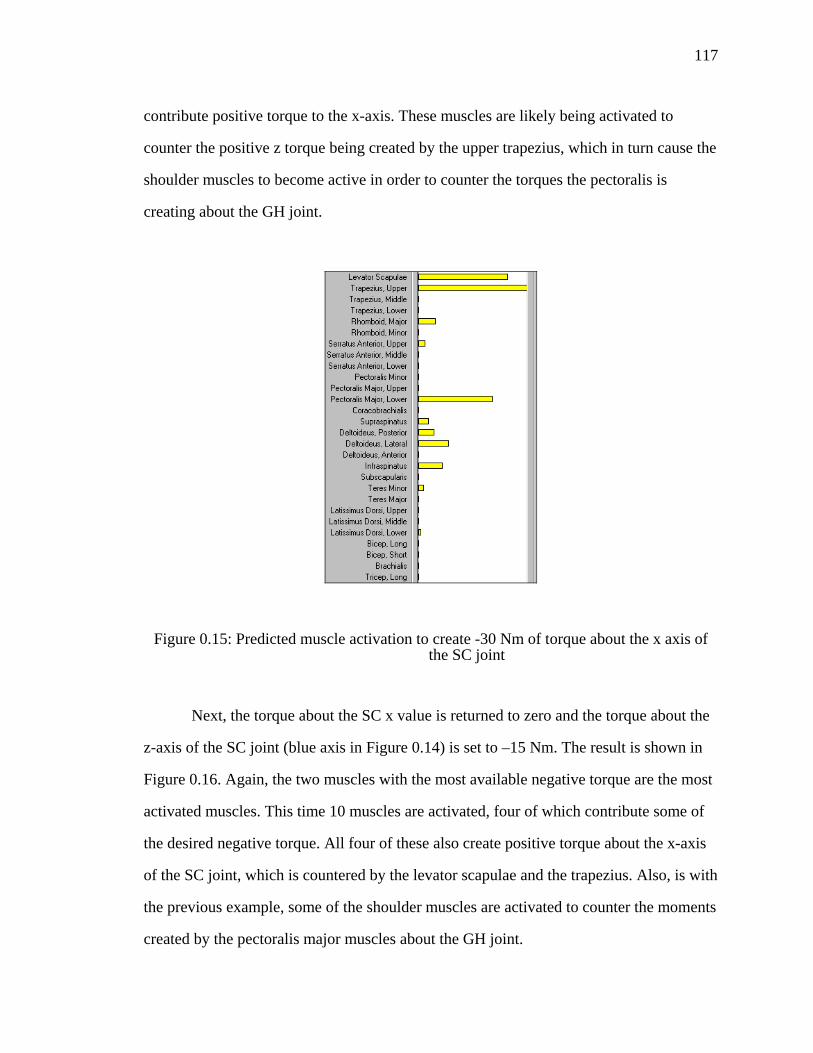
117

contribute positive torque to the x-axis. These muscles are likely being activated to

counter the positive z torque being created by the upper trapezius, which in turn cause the

shoulder muscles to become active in order to counter the torques the pectoralis is

creating about the GH joint.

Figure 0.15: Predicted muscle activation to create -30 Nm of torque about the x axis of the SC joint

Next, the torque about the SC x value is returned to zero and the torque about the

z-axis of the SC joint (blue axis in Figure 0.14) is set to –15 Nm. The result is shown in

Figure 0.16. Again, the two muscles with the most available negative torque are the most

activated muscles. This time 10 muscles are activated, four of which contribute some of

the desired negative torque. All four of these also create positive torque about the x-axis

of the SC joint, which is countered by the levator scapulae and the trapezius. Also, is with

the previous example, some of the shoulder muscles are activated to counter the moments

created by the pectoralis major muscles about the GH joint.

118

Figure 0.16: Predicted muscle activation to create -15 Nm of torque about the z-axis of the SC joint

Figure 0.17:Predicted muscle activation to create -15 Nm of torque about the z-axis of the GH joint

119

Now the torques about the SC will be set to zero and the torque about the z-axis

of the GH (blue axis in Figure 0.14) is set to –15 Nm resulting in Figure 0.17. This is the

type of torque that would be seen when a subject is trying to abduct the arm from the

torso. As expected the lateral deltoid is the most active muscle because it has the most

available negative torque about the z-axis. This muscle also creates some positive torque

that must be countered, which is likely why the anterior deltoid and supraspinatus are

active.

Figure 0.18: Predicted muscle activation to create -15 Nm of torque about the x-axis of the GH joint

The z torque about the GH joint is returned to zero and a –15 Nm torque is

applied to the x-axis of the GH joint (red axis in Figure 0.14), resulting in Figure 0.18.

This is the type of torque one would see if a subject was attempting to raise their elbow

up in front of their body. The anterior deltoid is the most activated muscle, which is

reasonable considering the amount of available negative torque is holds. The only other

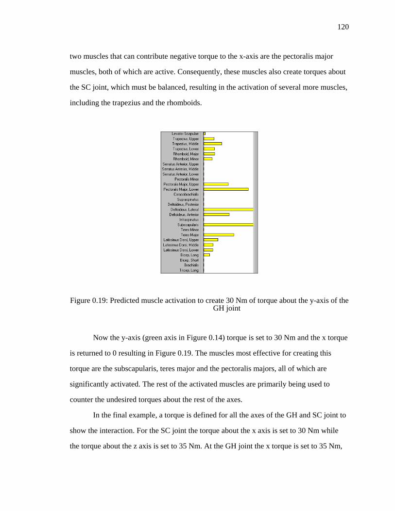
120

two muscles that can contribute negative torque to the x-axis are the pectoralis major

muscles, both of which are active. Consequently, these muscles also create torques about

the SC joint, which must be balanced, resulting in the activation of several more muscles,

including the trapezius and the rhomboids.

Figure 0.19: Predicted muscle activation to create 30 Nm of torque about the y-axis of the GH joint

Now the y-axis (green axis in Figure 0.14) torque is set to 30 Nm and the x torque

is returned to 0 resulting in Figure 0.19. The muscles most effective for creating this

torque are the subscapularis, teres major and the pectoralis majors, all of which are

significantly activated. The rest of the activated muscles are primarily being used to

counter the undesired torques about the rest of the axes.

In the final example, a torque is defined for all the axes of the GH and SC joint to

show the interaction. For the SC joint the torque about the x axis is set to 30 Nm while

the torque about the z axis is set to 35 Nm. At the GH joint the x torque is set to 35 Nm,

121

the y torque is set to –8 Nm and the z torque is set to 35 Nm. The result is shown in

Figure 0.20. One thing to note about this figure is that the activation levels of the muscles

usually only associated with the lower arm are also shown. Even though zero torque is

desired about the elbow several of these muscles are activated. This is because of the

tricep long is activated to help satisfy the torques about the shoulder, resulting in torque

generated on the ulna must which must be balanced.

Figure 0.20: Predicted muscle activation for selected torques about the GH and SC joint

For the last two examples the arm will be moved to two different postures and the

max torque for each muscle about both the SC and GH joint will be displayed to

demonstrate that the amount of available torque is dependent on the arm posture. In the

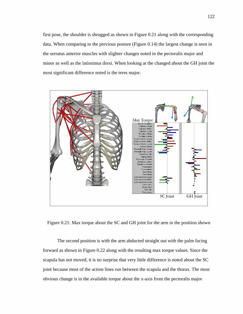
122

first pose, the shoulder is shrugged as shown in Figure 0.21 along with the corresponding

data. When comparing to the previous posture (Figure 0.14) the largest change is seen in

the serratus anterior muscles with slighter changes noted in the pectoralis major and

minor as well as the latissimus dorsi. When looking at the changed about the GH joint the

most significant difference noted is the teres major.

Figure 0.21: Max torque about the SC and GH joint for the arm in the position shown

The second position is with the arm abducted straight out with the palm facing

forward as shown in Figure 0.22 along with the resulting max torque values. Since the

scapula has not moved, it is no surprise that very little difference is noted about the SC

joint because most of the action lines run between the scapula and the thorax. The most

obvious change is in the available torque about the x-axis from the pectoralis major

123

action lines. When observing the changes about the GH joint, several changes can be

noted. In this position, the pectoralis major muscles have lost most of their capacity for

adducting the arm (positive torque about the z-axis) while the subscapularis capacity has

increased. The posterior deltoid is still the largest producer of positive torque about the x-

axis even thought its capacity has been reduced.

Figure 0.22: Max torque about the SC and GH joint for the arm in the position shown

Comparison with Experimental Data

In the previous sections we have demonstrated that our model produces

reasonable moments as far as direction and relative magnitude is concerned but how does

this compare to previous studies. Preliminary comparison was achieved by plotting the

moment arms of five action lines as the elbow moved from full extension (0°) to flexion

124

(120°) with the hand in the neutral orientation as shown in Figure 0.10. By doing this we

could compare our results to the results shown by Murray et al, who compared their

model and results to six other studies (Murray et al, 1995). The result is shown in Figure

0.23.

Figure 0.23: Comparison of our proposed model to previous studies

125

In order to compare the results, our model was scaled so it was similar in size to

the model presented by Murray et al. This was accomplished by uniformly scaling our

model until the length of the humerus was 30.3 cm as defined by Murray et al. It can be

observed from Figure 0.23 that the moment arms calculated by our model fit reasonably

well with the data presented in previous studies, especially the bicep, brachioradialis, and

pronator teres. The triceps, while maintaining a shape that is similar to the other data it

seems to like it needs to be shifted down about 1 cm. Because the shape is fairly

consistent with the previous studies this seems to indicate that the insertion point may

need to be adjusted. The brachialis moment arm starts out within the range of the

previous studies but then arc out too low at the end. Furthermore, its peak happens at

about 80° while the others either peak out at the end of the flexion. This seems to indicate

that the wrapping obstacles need to be adjusted.

Conclusions

In this chapter we have presented several examples of our model. In all the examples the

results were discussed and everything seems to be quite reasonable. In comparing our

moment arms to previous studies the data was shown to fit although some modifications

to the model could improve the fit. Further validation should include comparing the

predicted muscle levels to EMG studies and comparing the rest of the calculated moment

arms to experimental data. It should be noted that all the examples were able to run in

real time with the frame rates of the simulation of the never dropping below 60 frames

per second. While interacting with the joints or joint torques no obvious delay was

noticed between user input and data output.

126

CONCLUSIONS AND FUTURE WORK

Conclusions

This thesis has addressed the modeling and simulation of the musculoskeletal

system of the shoulder girdle and upper extremity by combining real time simulation

methods, advanced CAD modeling techniques, optimization methods, and new methods

for characterizing muscle wrapping about anatomical structures.

It has been shown that real time simulation is effectively used to simulate

kinematic movement of the upper limb while monitoring in real time predicted activation

level, moment arms, and available torque for all the muscles crossing the sterno-

clavicular, acromio-clavicular, gleno-humeral, ulna-humeral, and ulna-radial joints.

It has been shown that muscle activation is calculated in real time for every

individual muscle during motion from optimization based on a cost function and

constraints.

It has been shown that the system developed with 35 action lines and five bones

with 7 DOF representing the shoulder girdle and upper extremity can be simulated in a

3D interactive visual environment in real time allowing a user to explore various muscle

activation levels by changing loading conditions and joint angles.

It has been shown that optimization methods are well suited for the real time

prediction of muscle activation, particularly when appropriate cost functions are selected

It has been shown that significantly higher accuracy of muscle activation can be

obtained by accounting for muscle wrapping around underlying anatomical structures. A

new method for muscle wrapping was developed using floating via points, which has

allowed for the action line of the muscle to be more accurately represented by the

centroid line of the muscle.

127

A graphical user interface was developed to allow for a user to interact in real

time with the musculoskeletal system, changing the loading conditions and joint angles

while receiving feedback.

Compared with experimental results published in literature, it was shown that our

system yields results of the muscle moment arms are very consistent with published data.

Furthermore, when observing the actions of the muscles on the bones as predicted by our

model the result correlated with anatomical data.

Future Work

The amount of work that can be continued on this project is immense. This

section will attempt to summarize some of the work which we feel should be added next.

• Further verification is obviously a very important next step. This

verification should compare more muscle moment arm prediction to

literature and also start comparing activation prediction to previous

studies.

• Include ligament about the joints, which are used to stabilize the joints.

This is especially true for the elbow. In the current formulation, the

torques generated about the x and y axis of the elbow are ignored. If

ligaments are added to the model these could be used to resist torque about

these axes resulting in additional constraints for the optimization

formulations that stipulate that the torques generated about the x and y

axis must balance out to zero.

• Calculate and return joint reaction forces to the user. Not only could this

information be useful to the user but also it may be used as an additional

constraint by limiting the amount of force allowed within the joint.

Furthermore, this may be useful for including joint friction.

128

• Expand the model to the other arm and legs and reevaluate the

performance. The current model has not hindered real time performance

and it appears to have quite a bit of room to expand. Adding additional

action lines for some muscles may also be appropriate.

• Add robustness to the wrapping algorithm so that it can handle when

either the insertion or origin are moved within an object. Simply simply

moving the point or shrinking the obstacle until it is no longer within the

obstacle could handle this.

• Changing the color of the force lines based on activation level would be

useful for conceptualizing how the muscles reacting to different torque

loads and arm configurations. For instance, the lines would look blue if

there is no activation and slowly change to bright red as the muscle is

activated

• Vary the cost function of the prediction algorithm and observe the effect

of different conditions. Much improvement can be added to the muscle

prediction algorithm. More detailed muscle parameters should be used for

determining the maximum available force. Fatigue could possiblely be

incorporated with the formulation as presented by Komura et al (Komura

et al, 2000) while co-contraction could be addressed by the paper

presented by Foster et al (Foster et al, 2004).

• Now that we know force direction and location, this model could be

expanded to incorporate physics.

129

REFERENCES

Amis, A. A., Dowson, D., Wright, V. (1979) “Muscle strengths and Musculoskeletal geometry of the upper limb”, Engng Med., 8, 41-48

Amis, A.A., Dowson, D., Wright, V., (1980) “Elbow Joint Force Predictions for some Strenuous Isometric Actions”, J. Biomechanics, 13, 765

An, K. N., Hui, F. C., Morrey, B. F., Linscheid, R. L. and Chao, E. Y. (1981) Muscles “Across the elbow joint: A Biomechanical Analysis”. J. Biomechancs 14, 659-669

An, K. N., Kwan, B. M., et al., (1984) “Determination of muscle and joint forces: a new technique to solve the indeterminate problem.” Journal of Biomedical Engineering, 106 (4), 164-367

An, K. N., Takahashi, K. Harrigan, T. P., Chao, E. Y. (1984) “Determination of muscle orientation and moment arms”, J. biomech. Engn, 106, 280-282

Anderson, F.C., Pandy, M.G., (1999) “A Dynamic Optimization Solution for Vertical Jumping in Three Dimensions.” Computer Methods in Biomechanics and Biomedical Engineering, 2, 201-231

Berme, N., Heydinger, G., and Cappozzo, A., (1987) “Loads Transmitted at the Anatomical Joints”. In A. Morechi (ed) Biomechanics of Engineering: Modeling, Simulation, Control, Wien, New York

Blemker, S.S., Delp, S. L., (2005) “Three-dimensional representation of complex muscle architectires and geometries” Annals of Biomedical Engineering, 33, 5, 661-673

Chadwick, E.K., Nicol, A.C., (2000) “Elbow and wrist joint contact forces during occupational pick and place activities.” J. Biomechanics, 33 (5), 591-600

Chao, E.Y. S., (2003) “Graphic-based musculoskeletal model for biomechanical analyses and animation”, Medical Engieering & Physics, 25, 201-212

Crowninshield, R.D., (1978) “Use of optimization techniques to predict muscle forces”, Transactions of the ASME, 100, 72

Crowninshield, R.D., Brand, R.A., (1981) “A physiological based criterion of muscle force prediction in locomotion.” J. Biomechanics 14 (11), 793-801

Davy, D.T., Audu, M.L., (1987) “A dynamic optimization technique for predicting muscle forces in the swing phase of gait”, J. Biomechanics, 20, 187-201

Delp, S. L., Loan, J. P. (1995) “A graphics-based software to develop and analyze models of musculoskeletal structures”, Comput. Biol. Med. 25, 1, 21-34

DeLucam C.J., Forrest, W.J., (1973) “Force analysis of individual muscles acting simultaneously on the shoulder during isometric abduction”, J. Biomechanics, 6, 385-393

Dvir, Z. and Berme, N. (1978), “The Shoulder Complex in Elevation of the Arm: A Mechanism Approach”, Journal of Biomechanics, 11, 219-255

130

Engin, A. E. (1984), “On the Theoretical Modelling of Human Joints”. In Mathematical Modelling in Science and Technology (ed. J. R. Avula), Pergamon Press, New York, pp. 560-565

Engin, E. (1980), “On the Biomechanics of the Shoulder Complex”, Journal of Biomechanics, 13, 575-590

Forster, E., Simon, U., Augat, P., Claes, L., (2004) “Estension of a state-of-the-art optimization criterion to predict co-contraction”, J. Biomechanics, 37, 577-581

Gill, P. E., Murray, W., Saunders, M. A., (2002) “SNOPT: An SQP algorithm for large-scale constrained optimization”, Siam J. Optim., 12, 4, 979-1006

Glitsch, U., Baumann, W., (1997) “The three-dimensional determination of internal loads in the lower extremity.” J. Biomechanics, 30 (11-12), 1123-1131

Happee, R., (1994) “Inverse dynamic optimization including muscular dynamics, a new simulation method applied to goal directed movements.” J. Biomechanics 27 (7), 953-960

Helm, F. C. T, Veenbaas, R. (1991), “Modelling the Mechanical Effect of Muscles with Large Attachment Sites: Application to the Shoulder Mechanism”, Journal of Biomechanics, 27, 1151-1163

Helm, F. C. T. (1994), “A Finite Element Musculoskeletal Model of the Shoulder Mechanism”, Journal of Biomechanics, 27, 551-569

Helm, F. C. T. and Pronk, G. M. (1995). “Three-Dimensional Recording and Description of Motions of the Shoulder Mechanism”, Journal of Biomechanical Engineering, 117, 27-40

Hogfors, C., Sigholm, G., and Herberts, P. (1987), “Biomechanical Model of the Human Shoulder – I. Elements”, Journal of Biomechanics, 20, 157-166

Jackson, K. M., Joseph, J., Wyard, S. J., (1977) “Sequential muscular contraction”, J. Biomechanics,10, 97-100

Jenesn, R. H. and D. T. Davy (1975) “An Investigation of Muscle Lines of Action About the Hip: A Centroid Line Approach VS the Straight Line Approach”. J. Biomechanics 8, 103-110

Kaufman, K.R., An, K.W., et al (1991) “Physiological prediction of muscle forces-I. Theoretical formulation.” Neuroscience 40 (3) 781-792

Kim, J., Abdel-Malek, K., Yang, J., Farrell, K., Nebel, K., (2005) “Optimization-Based dynamic motion simulation and energy expenditure prediction for a digital human” SAE Digital Human Modeling for Design and Engineering, June, Iowa City, IA USA.

Kimura, T., Shinagawa, Y., Kunni, T. L., (2000) “Creating and retargeting motion by the musculoskeletal human body model”, The Visual Computer, 16, 254-270

Kinzel, G. L. and L. J. Gutkowski (1983), “Joint Models, Degrees of Freedom, and Anatomical Motion of Measurements”, Journal of Biomechanical Engineering, 105, 55-61

131

Li, G., Kaufman, K.R., et al., (1999) “Prediction of antagonistic muscle forces using inverse dynamic optimization during flexion/extension of the knee.” Journal of Biomedical Engineering 121 (3) 316-322

Li, G., Pierce, J. E., Herndon, J.H., (2004) “A global optimzation method for prediction of muscle forces of human musculoskeletal system.” J. Biomechancs, Accepted 2004

Maurel, W., Thalmann, D. (1999), “A case study on human upper limb modeling for dynamic simulations”, Computer Methods in Biomechanics and Biomedical Engineering, Vol 2, No. 1, pp 65-82

Maurel, W., Thalmann, D., Hoffmeyer, P., Beylot, P., Gingins, P., Karla, P., Thalmann, , N. (1996), “A Biomechanical Musculoskeletal Model of Human Upper Limb for Dynamic Simulation”, EGCAS ’96, 7th Eurographics Workshop on Computer Animation and Simulation ’96 (Springer Poitiers 1996), 121-136

Mikosz, R. P., McKersie, R., Berg, R. Snitovsky, P., Lobick, J., Logue, S., Andersson, G. B. J. and Andriacchi, T. P (1988) “Muscle Lines of Action in the Lower Extremity: A cetntroid line approach vs the straight line approach”. Proc. 12th Am Soc Biomechanics. Pp 30-31, Urbana-Champaign, IL.

Murray, W. M., Delp, S. L., Buchanan, T. S. (1995) “Variation of muscle moment arms with elbow and forearm position”, J. Biomechanincs, 28, 5, 513-525

Pedotti, A., Krishnan, V. V., et al (1978) “Optimization of the muscle force sequencing in human locomotion.” Mathematical Biosciences 38, 57-76

Poppen, N.K., Walker, P.S., (1978) “Forces at the glenohumeral joint in abduction”, Clin. Orthop Rel. Res.,135, 165-170

Praagman, M. Chadwick, E.K.J., Helm, F.C.T. van der, Veeger, H.E.J. (2004) “The relationship between two different mechanical cost functions and muscle oxygen consumption.” J. Biomechanics, Accepted 2004.

Raikova, R. (1992), “A General Approach for Modelling and Mathematical Investigation of the Human Upper Limb”, Journal of Biomechanics, 25, 857-867

Raikova, R. (1996) “A model of the flexion – extension motion in the elbow joint – some problems concerning muscle forces modeling and computation” J. Biomechanics, 29, 6, 763-772

Seireg, A. and Avikar, R.J. (1973) “A mathematical model for the evaluation of forces in the lower extremeties of the musculoskeletal system.” J. Biomechanics 6, 313-326

Tozeren, A., (2000) Human Body Dynamic, N.Y.: Springer-Verlag

Van Zuylen, E. J., van Zulzen, A., Denier van der Gon, J. J. (1988), “A biomechanical model for flexion torques of human arm muscles as a function of elbow angle”, J. Biomechanics, 21, 183-190

Veeger, H. E. J., Yu, B., An, K. N., Rozendal, R. H., (1996) “Parameters for modeling the upper extremeity”, J. Biomechanics, 30, 6, 1997

132

Wickens, C. D., Baker, P. (1995) “Cognative Issues in Virtual Reality”. Virtual Environments and Advanced Interface Design (ed. W. Barfield and T.A. Furness III), Oxford University Press. 514-541

Winters, J. M., Klewendo, D. G. (1993) “Effect of initial upper-limb alignment on muscle contributions to isometric strength curves”, J. Biomechanics, 26, 143-153

133

CHAPTER 1: INTRODUCTION ........................................................................................1 1.1 Overview .....................................................................................................1 1.2 Past Work ....................................................................................................1 1.3 Objectives ...................................................................................................3 1.4 Conclusion ..................................................................................................4

CHAPTER 2: TERMINOLOGY, METHODS AND MATHEMATICS............................5 2.1 Nomenclature ..............................................................................................5 2.2 Medical Terminology .................................................................................5 2.3 Terminology ...............................................................................................7 2.4 Optimization ...............................................................................................8 2.5 Conclusion ..................................................................................................9

CHAPTER 3: PROBLEM FORMULATION ...................................................................10 3.1 Introduction ...............................................................................................10 3.2 Torque – Force Relationship ....................................................................10 3.3 Applying the Torque-Force Relationship to the Body .............................12

3.3.1 Musculoskeletal System .................................................................13 3.3.2 Mechanical System .........................................................................13

3.4 Optimization .............................................................................................16 3.4.1 Optimization Example ....................................................................18

3.5 Proposed Formulation ...............................................................................21 3.6 Model Requirements .................................................................................22

CHAPTER 4: MODELING ...............................................................................................23 4.1 Introduction ...............................................................................................23 4.2 Anatomy ...................................................................................................23 4.3 Digital Representation of the Arm ............................................................29

4.3.1 Kinematic Model ............................................................................31 4.3.2 Attaching the Muscles ....................................................................39

4.4 Conclusion ................................................................................................54

CHAPTER 5: MODELING OF MUSCLE WRAPPING ..................................................55 5.1 Introduction ...............................................................................................55 5.2 Problem Formulation ................................................................................59 5.3 Proposed Solution .....................................................................................60

5.3.1 Wrapping Algorithm for a Sphere ..................................................61 5.3.2 Wrapping Algorithm for a Cylinder ...............................................64 5.3.3 Multiple Obstacle Wrapping ..........................................................70

5.4 Examples ...................................................................................................72 5.4.1 Spherical Wrapping ........................................................................72 5.4.2 Cylindrical Wrapping .....................................................................75 5.4.3 Multiple Obstacle Wrapping ..........................................................78

5.5 Discussion .................................................................................................81 5.6 Conclusions ...............................................................................................82

CHAPTER 6: REAL TIME INTERACTION ...................................................................83 6.1 Introduction ...............................................................................................83 6.2 Software ....................................................................................................83 6.3 Creating User Interaction ..........................................................................86 6.4 Data Feedback ..........................................................................................87

134

6.4.1 Moment Arm Display .....................................................................88 6.4.2 Max Torque Display .......................................................................90 6.4.3 Activation Display ..........................................................................92

6.5 Conclusion ................................................................................................93

CHAPTER 7: RESULTS AND DISCUSSION .................................................................94 7.1 Introduction ...............................................................................................94 7.2 Lower Arm ................................................................................................95 7.3 Pectoral Girdle ........................................................................................113 7.4 Comparison with Experimental Data ......................................................123 7.5 Conclusions .............................................................................................125

CHAPTER 8: CONCLUSIONS AND FUTURE WORK ...............................................126 8.1 Conclusions .............................................................................................126 8.2 Future Work ............................................................................................127

CHAPTER 9: REFERENCES .........................................................................................129

135

Figure 2.1: Primary planes of the body used for spatial description ...................................6

Figure 2.2: Notation describing anatomical movement .......................................................7

Figure 3.1: Torque calculation ...........................................................................................10

Figure 3.2: Example of the force-torque relationship ........................................................11

Figure 3.3: Example of multiple forces creating torque ....................................................11

Figure 3.4: Major muscles of the upper arm ......................................................................12

Figure 3.5: Medial bicep brachii ........................................................................................13

Figure 3.6: Force from bicep .............................................................................................14

Figure 3.7: Muscle force components ................................................................................14

Figure 3.8: Effect of joint angle. Note the shortening if the stabilizing component and the lengthening of the rotational component as the elbow is flexed ..................15

Figure 3.9: Three muscles acting on the lower arm ...........................................................16

Figure 4.1: Axial skeleton (left) and appendicular skeleton (right) ...................................23

Figure 4.2: Example of muscles attaching to the bones .....................................................24

Figure 4.3: Bones of the right arm .....................................................................................25

Figure 4.4: Muscles of the shoulder ...................................................................................26

Figure 4.5: Muscles of the shoulder and arm .....................................................................27

Figure 4.6: Muscles of the shoulder and arm .....................................................................28

Figure 4.7: Muscles of the shoulder and arm .....................................................................29

Figure 4.8: Muscles of the arm ..........................................................................................30

Figure 4.9: Hierarchy of the bones in the arm ...................................................................31

Figure 4.10: Joints of the arm ............................................................................................32

Figure 4.11: Guide points on the scapula...........................................................................33

Figure 4.12: Vector used to rotate the scapula ...................................................................34

Figure 4.13: Heirarchy of joint frames in a 3DOF joint ....................................................35

Figure 4.14: Euler rotation order for a 3DOF joint. Note that all the frames are separated just for clarity. In the model they coincide. ..............................................35

136

Figure 4.15: Sterno-clavicular reference (left) and local frame (right) .............................37

Figure 4.16: Acromio-clavicular reference (left) and local frame (right) ..........................37

Figure 4.17: Gleno-humeral reference (left) and local frame (right) .................................38

Figure 4.18: Ulno-humeral reference and local frame .......................................................38

Figure 4.19: Ulno-radial reference and local frame ...........................................................39

Figure 4.20: Effects of muscle wrapping as applied to the biceps .....................................40

Figure 4.21: Trapezius and its action lines ........................................................................41

Figure 4.22: Levator scapulae muscle and action line .......................................................42

Figure 4.23: Trapezius muscle, action lines and wrapping obstacles ................................42

Figure 4.24: Rhoboids muscles, action lines and wrapping obstacle ................................43

Figure 4.25: Serratus anterior muscles, action lines and wrapping obstacles ....................44

Figure 4.26: Pectoralis minor muscle, action lines and wrapping obstacle .......................44

Figure 4.27: Pectoralis major muscle, action lines and wrapping obstacles ......................45

Figure 4.28: Coracobrachialis muscle, action line and wrapping obstacle ........................45

Figure 4.29: Supraspinatus muscle, action line and wrapping obstacle ............................46

Figure 4.30: Deltoideus muscle, action lines and wrapping obstacles ..............................46

Figure 4.31: Infraspinatus muscle, action line and wrapping obstacle ..............................47

Figure 4.32: Subacapularis muscle, action line and wrapping obstacle ............................47

Figure 4.33: Teres Minor muscle, action line and wrapping obstacles .............................48

Figure 4.34: Teres Major muscle, action line and wrapping obstacles ..............................48

Figure 4.35: Latissimus dorsi muscle, action lines and wrapping obstacles .....................49

Figure 4.36: Bicep brachii muscles, action lines and wrapping obstacles .........................49

Figure 4.37: Triceps major muscles, action lines and wrapping obstacle .........................50

Figure 4.38: Brachialis muscle, action line and wrapping obstacles .................................51

Figure 4.39: Brachioradialis muscle, action line and wrapping obstacles .........................51

Figure 4.40: Pronator teres muscle, action line and wrapping obstacles ...........................52

Figure 4.41: Supinator muscle, action lines and wrapping obstacles ................................52

137

Figure 4.42: Anconeus muscle, action line and wrapping obstacle ...................................53

Figure 4.43: All modeled action lines ................................................................................54

Figure 5.1: Attachment of the long head of the bicep ........................................................55

Figure 5.2: Straight line model for the short head of the bicep .........................................56

Figure 5.3: Bicep action line intersecting with the humerus .............................................57

Figure 5.4: Triceps action lines with fixed via points about the elbow .............................58

Figure 5.5: Lower action line of the trapezius with fixed via points on the medial edge of the scapula ....................................................................................................59

Figure 5.6: Example of wrapping about a sphere ..............................................................60

Figure 5.7: Wrapping about a sphere in the sphere’s x-y plane which also represents the AL plane ............................................................................................62

Figure 5.8: Wrapping about a cylinder ..............................................................................65

Figure 5.9: Wrapping about a cylinder in the cylinder's x-y plane ....................................66

Figure 5.10: Difference between wrapping if negative or a positive cross product is allowed ......................................................................................................................68

Figure 5.11: Wrapped line viewed in u-v coordinates .......................................................68

Figure 5.12: Example of wrapping around two objects .....................................................71

Figure 5.13: Logic for spherical wrapping example ..........................................................72

Figure 5.14: Sphere wrapping example .............................................................................73

Figure 5.15: Sphere wrapping example .............................................................................74

Figure 5.16: Sphere wrapping example .............................................................................74

Figure 5.17: Sphere wrapping example .............................................................................75

Figure 5.18: Logic for cylinder wrapping example ...........................................................75

Figure 5.19: Cylinder wrapping example ..........................................................................76

Figure 5.20: Cylinder wrapping example ..........................................................................77

Figure 5.21: Cylinder wrapping example ..........................................................................77

Figure 5.22: Cylinder wrapping example ..........................................................................78

Figure 5.23: Setup for multiple obstacle wrapping example .............................................78

Figure 5.24: Logic for multiple obstacle wrapping ...........................................................79

138

Figure 5.25: Multiple object wrapping example ................................................................80

Figure 5.26: Multiple object wrapping example ................................................................80

Figure 5.27: Sphere moved while simulation is paused to determine how long the solution takes to converge.........................................................................................81

Figure 6.1: Interaction between programs .........................................................................85

Figure 6.2: Joint torque user interface. For the joints with more than 1DOF the sliders are arranged such that the top slider is torque about x, middle slider is torque about y and the bottom slider is torque about z. ............................................87

Figure 6.3: Moment Arms of muscles crossing the sterno-clavicular joint .......................88

Figure 6.4: Moment Arms of muscles crossing the acromio-clavicular joint (left) and the gleno-humeral joint (right) ...........................................................................89

Figure 6.5: Moment arms of muscles crossing the ulno-humeral joint (left) and the ulno-radial joint (right) .............................................................................................90

Figure 6.6: Max torque of muscles crossing the sterno-clavicular joint ............................91

Figure 6.7: Max torque of muscles crossing the acromio-clavicular joint (left) and the gleno-humeral joint (right) ..................................................................................91

Figure 6.8: Max torque of muscles crossing the ulno-humeral joint (left) and the ulno-radial joint (right) .............................................................................................92

Figure 6.9: Predicted activation levels ...............................................................................93

Figure 7.1: Max muscle stress (kPa) and PCSA (cm2) data used in the examples ............94

Figure 7.2: Action lines for the lower arm .........................................................................95

Figure 7.3: Action lines wrapping around the elbow. From left to right: elbow fully extended with hand supinated, elbow halfway flexed with hand supinated, elbow fully flexed with hand pronated .....................................................................96

Figure 7.4: Example 1; Hand is neutral and the elbow if fully extended. The charts show the moment arms and max torque about each joint for all 11 action lines of the lower arm ........................................................................................................97

Figure 7.5: Predicted muscle activation for various torques..............................................98

Figure 7.6: Example 2; Hand is neutral and the elbow if fully flexed. The charts show the max torque about each joint for all 11 action lines of the lower arm ......101

Figure 7.7: Predicted muscle activation for various torques............................................103

Figure 7.8: Predicted muscle activation levels for the muscles of the lower arm with a desired torque of 23.1 Nm about the UH joint and 2 Nm about the UR joint .....103

139

Figure 7.9: Predicted muscle activation levels for the muscles of the lower arm with a desired torque of 36.7 Nm about the UH joint and 2.5 Nm about the UR joint .........................................................................................................................105

Figure 7.10: Example where the elbow is flexed to the position shown while the hand is neutral. The graphs display the max torque that each action can apply about each joint and the predicted activation level of each muscle for two different torque configurations. ..............................................................................107

Figure 7.11: Example where the elbow is flexed to the postion shown while the hand is pronated. The graphs display the max torque that each action can apply about each joint and the predicted activation level of each muscle for two different torque confuguratons.........................................................................110

Figure 7.12: Example where the elbow is flexed to the postion shown while the hand is spinated. The graphs display the max torque that each action can apply about each joint and the predicted activation level of each muscle for two different torque confuguratons.........................................................................111

Figure 7.13: Action lines of the pectoral girdle ...............................................................113

Figure 7.14: Example of the pectoral girdle. Graphs display max torque about the SC and GH joint ......................................................................................................114

Figure 7.15: Predicted muscle activation to create -30 Nm of torque about the x axis of the SC joint..................................................................................................117

Figure 7.16: Predicted muscle activation to create -15 Nm of torque about the z-axis of the SC joint..................................................................................................118

Figure 7.17:Predicted muscle activation to create -15 Nm of torque about the z-axis of the GH joint ........................................................................................................118

Figure 7.18: Predicted muscle activation to create -15 Nm of torque about the x-axis of the GH joint .................................................................................................119

Figure 7.19: Predicted muscle activation to create 30 Nm of torque about the y-axis of the GH joint ........................................................................................................120

Figure 7.20: Predicted muscle activation for selected torques about the GH and SC joint .........................................................................................................................121

Figure 7.21: Max torque about the SC and GH joint for the arm in the position shown ......................................................................................................................122

Figure 7.22: Max torque about the SC and GH joint for the arm in the position shown ......................................................................................................................123

Figure 7.23: Comparison of our proposed model to previous studies .............................124