1

Electromagnetic Sensing for Space-borne Imaging

Lecture 6Antenna Lore, Transmission and Reception Patterns, Phased Arrays,Sparse Aperture Theorem

2

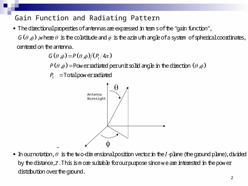
Gain Function and Radiating Pattern

The directional properties of antennas are expressed in terms of the "gain function",

, , where is the colatitude and is the azimuth angle of a system of spherical coordinates,

centered on

G

the antenna.

, , 4

, Power radiated per unit solid angle in the direction ,

Total power radiated

In our notat

t

t

G P P

P

P

ion, is the two-dimensional position vector in the -plane (the ground plane), divided

by the distance, . This is more suitable for our purpose since we are interested in the power

distributi

I

z

on over the ground.

Antenna Boresight

3

Gain Function and Radiating Pattern

The maximum value of the gain function is called the "gain", denoted by

is the greatest factor by which the power transmitted in a given direction

can be increased by using the antenna inst

M

M

G

G

ead of an isotropic radiator.

The transmitting pattern of an antenna is the surface

,

A cross section of this surface in any plane that includesM

Gr

G

the origin is called

the "polar diagram" of the antenna in this plane

4

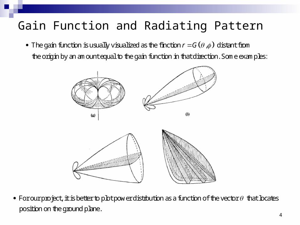
Gain Function and Radiating Pattern

The gain function is usually visualized as the finction , distant from

the origin by an amount equal to the gain function in that direction. Some examples:

r G

For our project, it is better to plot power distrbution as a function of the vector that locates

position on the ground plane.

5

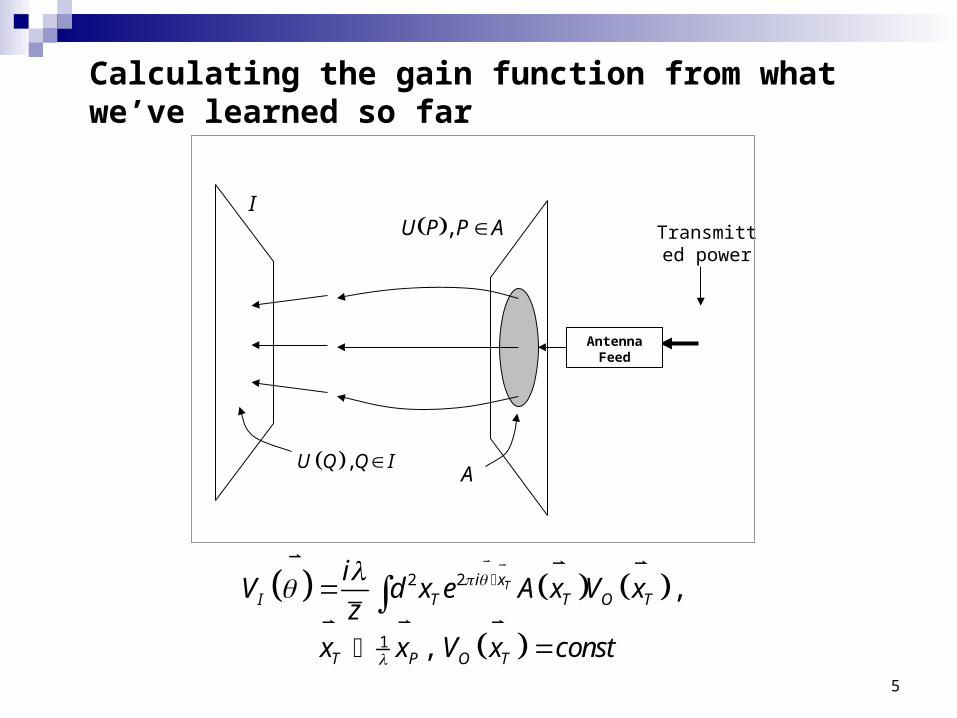
,U Q Q I

U P , P A Transmitted power

I

A

Antenna Feed

Calculating the gain function from what we’ve learned so far

22

1

,

,

Ti xI T T O T

T P O T

iV d x e A x V x

zx x V x const

6

Calculating the gain function from what we’ve learned so far

222 2 22

222 22 2

The total power is:

Using Parseval's theorem, this becomes:

T

T

i xI O T T

i xt O T T

P V V d x e A xz

P V d d x e A xz

22 2

222 2

Finally, combining and into 4 , we get:

4 T

t O T T

t t

i xT T T T

P V d x A xz

P P G P P

G d x e A x d x A x

7

Calculating the gain functionExample: Circular aperture of diameter D

1 12 2

1 12 2

2

The aperture function is:

1, 1,

0, 0,

Considering the integral , if we replace by , then:

T

P T

P T

P T

i xT T T

x D x DA x A x

x D x D

Ddx e A x x u

d

2 122 2

12

2

22

1,exp 2

0,

=

The integral is obviously . Hence4

Ti xT T

T T

uD Dx e A x d u i u

u

D Djinc

Dd x A x

22 2

22

becomes:

Finally, combining and into 4 , we get:

16

t O T T

t t

G

P V d x A xz

P P G P P

D DG jinc

8

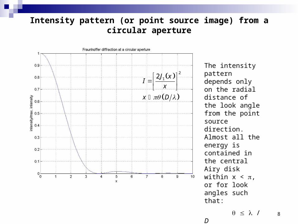
Intensity pattern (or point source image) from a circular aperture

2

12J xI

x

x D

The intensity pattern depends only on the radial distance of the look angle from the point source direction. Almost all the energy is contained in the central Airy disk within x < , or for look angles such that:

/ D

9

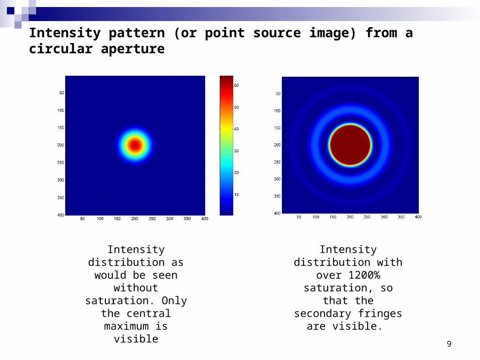
Intensity pattern (or point source image) from a circular aperture

Intensity distribution as would be seen without

saturation. Only the central maximum is

visible

Intensity distribution with over 1200%

saturation, so that the secondary fringes are

visible.

10

Receiving Pattern

Now consider the antenna as a receiving device. If is the power flux of the incoming

field then the power absorbed in unit solid angle about a given direction is:

S

,

where , is the "receiving cross section" or "absorption cross section".

Like the gain function, , , is usually represented by the surface:

r r

r

r

P SA

A

A

,

If is the maximum value of , then the "receiving pattern" is defined as:

,

Beca

r

rM r

r rM

r A

A A

r A A

2

use of reciprocity:

, ,

and:

, ,4

r

M rM

r

G A

G A

A G

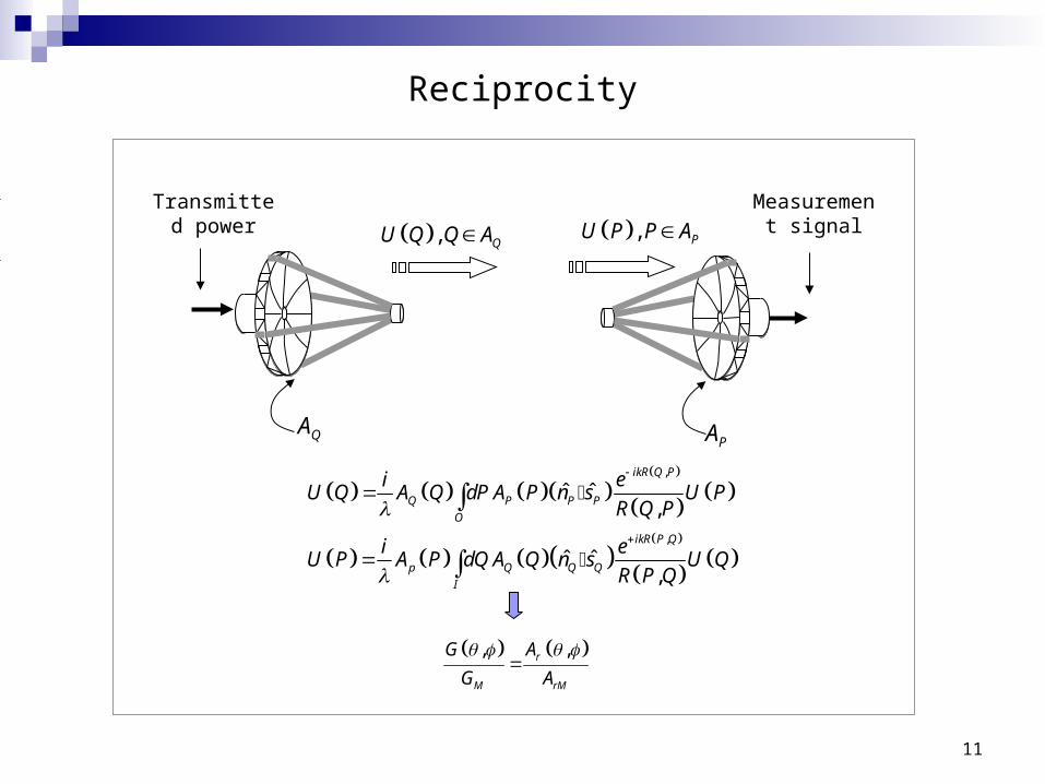
11

Reciprocity

,

,

ˆ ˆ,

ˆ ˆ,

ikR Q P

Q P P P

O

ikR P Q

p Q Q Q

I

i eU Q A Q dP A P n s U P

R Q P

i eU P A P dQ A Q n s U Q

R P Q

, PU P P AMeasurement

signal

AP

Transmitted power , QU Q Q A

AQ

, , r

M rM

G A

G A

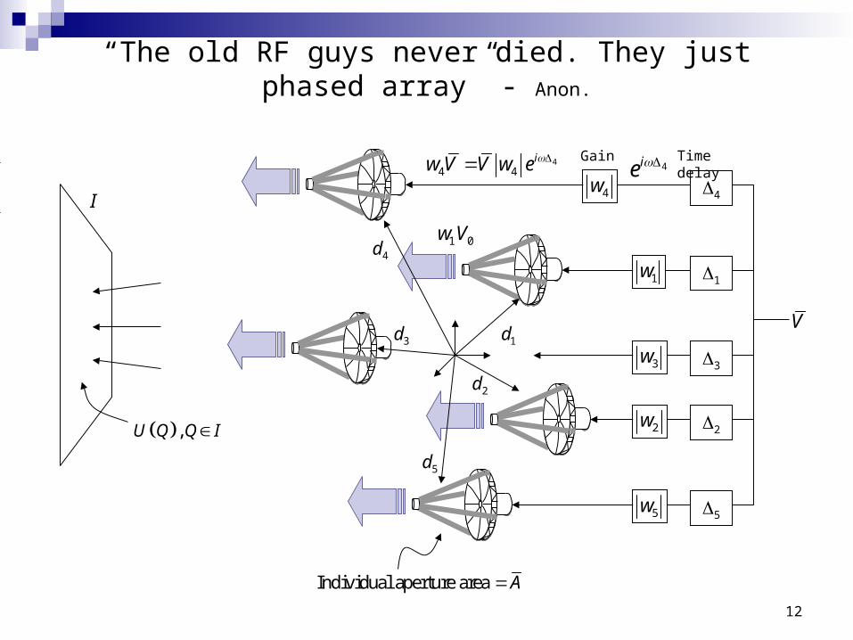
12

“The old RF guys never died. They just phased array” - Anon.

,U Q Q I

I

1d

2d

5d

4d

3d

4ie 44 4

iw V V w e

1 0w V

V

4

Time delay

1

3

2

5

4w

5w

2w

3w

1w

Gain

Individual aperture area A

13

Phased Array – Complex Amplitude on the Ground Plane

22

1

1

1

1

,

,

Since

Therefore:

Ti xI T T O

T P O

N

P n R P nn

N

T P T n R T nn

iV d x e A x V

zx x V V A

A x w A x d

x x A x w A x d

22

1

T

Ni x

I n T R T nn

i VV w d x e A x d

z A

14

Phased Array – Complex Amplitude on the Ground Plane

2 22

1

1

In the n integral, let :

,

And letting 2 :

n T

n

thT T n

Ni d i x

I n T R Tn

Nik d

I nn

x x d

i VV w e d x e A x

z A

k

V R w e

22

is the complex amplitude (on the ground plane) produced by

a single aperture

Ti xT T

i VR d x e A x

z A

R

15

Phased Array – Complex Amplitude on the Ground Plane

1

1

is called the

The AF can also be expressed as

where

n

n

Nik d

I nn

Nik d

nn

T

V R w e

w e

k

w v

Array Factor (AF)

1

2

is called the

N

ik d

ik d

ik d

e

ek

e

v

Steering Vector

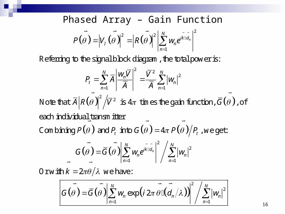
16

Phased Array – Gain Function

22 2

1

2 22

1 1

22

Referring to the signal block diagram, the total power is:

Note that is 4 times the gain functi

n

Nik d

I nn

N Nn

t nn n

P V R w e

w V VP A w

A A

A R V

22

1 1

22

1

on, , of

each individual transmitter

Combining and into 4 , we get:

Or with 2 we have:

exp 2

n

t t

N Nik d

n nn n

N

n n nn

G

P P G P P

G G w e w

k

G G w i d w

1

N

n

17

Simple 1-D Array Example

2

1

Equally spaced array along the axis: = ,0 , 1,...,

Uniform weights: 1, 1,...,

Isotropic emitters: 1

1 exp 2

After some algebra, one

P n

n

N

xn

x d n n N

w n N

G

G i nN

2

can show that this expression is identical to:

sin1

sin

x

x

NG

N

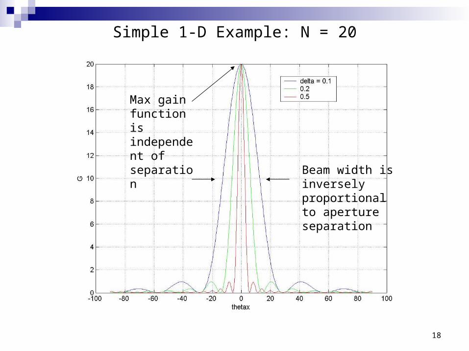
18

Simple 1-D Example: N = 20

Beam width is inversely proportional to aperture separation

Max gain function is independent of separation

19

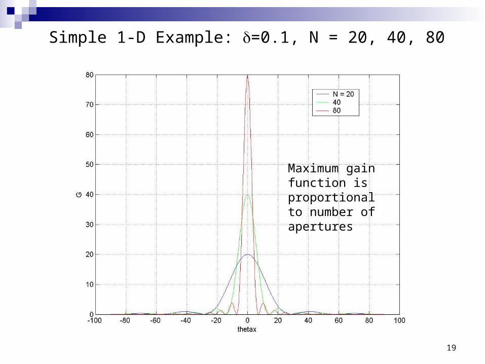
Simple 1-D Example: =0.1, N = 20, 40, 80

Maximum gain function is proportional to number of apertures

20

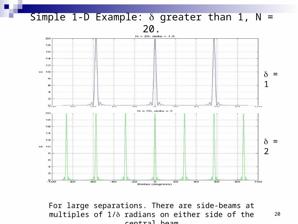
Simple 1-D Example: greater than 1, N = 20,

For large separations. There are side-beams at multiples of 1/ radians on either side of the central beam

= 1

= 2

21

Power density on the ground - 1-D Case

Early in the history of this technology, people thought that if they increased the transmitter separations and thereby decreased the beam width, they would increase the power density of the central beam. This is false.

In the 1-D case, we see that: Doubling the separation does decrease the beam width by 2. But the max value of G (which is proportional to power density)

is independent of separation. Therefore the total power in the main beam is smaller by a factor

of 2. Total overall power remains the same. Power lost from the main

beam reappears in side-beams

Analogous results hold for a general 2-D array

22

The Sparse (or Thinned) Aperture Theorem

In the 2-D case: Increasing the separation by a factor R decreases the beam

width by the same factor. But the max value of G (which is proportional to power density)

is independent of separation. Therefore the total power in the main beam is smaller by a factor

of 1/R2. Total overall power remains the same. Power lost from the main

beam reappears in the side-beams These observations form the “Sparse Aperture

Theorem”, aka “Sparse Aperture Curse” *

*Robert L. Forward, “Roundtrip Interstellar Travel Using Laser Pushed Lightsails, J. Spacecraft and Rockets, Vol. 21, No. 2, Mar.-Apr. 1984, p.190.