Embed Size (px)
Citation preview
1
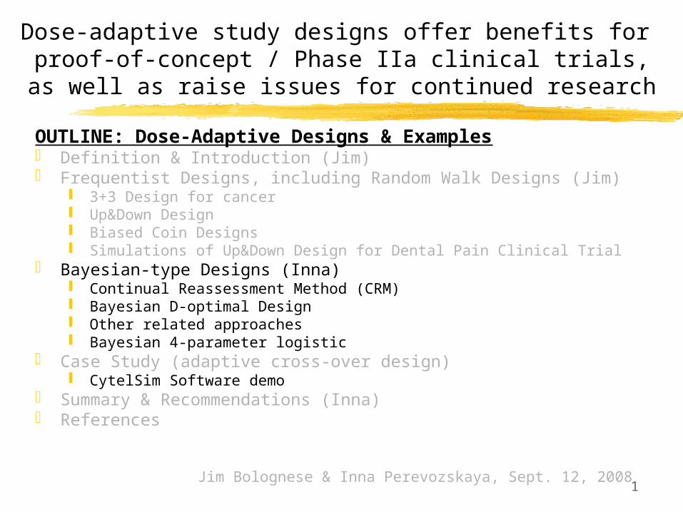
Dose-adaptive study designs offer benefits for proof-of-concept / Phase IIa clinical trials,
as well as raise issues for continued research
OUTLINE: Dose-Adaptive Designs & Examples Definition & Introduction (Jim) Frequentist Designs, including Random Walk Designs (Jim)
3+3 Design for cancer Up&Down Design Biased Coin Designs Simulations of Up&Down Design for Dental Pain Clinical Trial
Bayesian-type Designs (Inna) Continual Reassessment Method (CRM) Bayesian D-optimal Design Other related approaches Bayesian 4-parameter logistic
Case Study (adaptive cross-over design) CytelSim Software demo
Summary & Recommendations (Inna) References
Jim Bolognese & Inna Perevozskaya, Sept. 12, 2008
01/25/2006 Innovative Clinical Drug Development Conference
2
Continual Reassessment Method (CRM)
Most known Bayesian method for Phase I trials Underlying dose-response relationship is described by a 1-
parameter function family For a predefined set of doses to be studied and a binary response,
estimates dose level (MTD) that yields a particular proportion (P) of responses
CRM uses Bayes theorem with accruing data to update the distribution of MTD based on previous responses
After each patient’s response, posterior distribution of model parameter is updated; predicted probabilities of a toxic response at each dose level are updated
The dose level for next patient is selected as the one with predicted probability closest to the target level of response
Procedure stops after N patients enrolled Final estimate of MTD: dose with posterior probability closest to P
after N patients The method is designed to converge to MTD
3
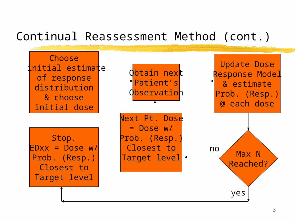
Continual Reassessment Method (cont.)
Choose initial estimate
of response distribution& choose
initial dose
Obtain nextPatient’s
Observation
Update DoseResponse Model
& estimateProb. (Resp.)@ each dose
Max NReached?
Next Pt. Dose= Dose w/
Prob. (Resp.)Closest to
Target levelno
Stop.EDxx = Dose w/
Prob. (Resp.)Closest to
Target level
yes
4
Escalation With Overdose Control (EWOC) Bayesian Design
Assigns doses similarly to CRM, except for overdose control predicted probability of next assignment exceeding MTD is controlled (Bayesian
feasible design) this distinction is particularly important in oncology
Assumes a model for the dose-response curve in terms of two parameters: MTD probability of response at dose D1
EWOC updates posterior distribution of MTD based on this two-parameter model
Free software available here: http://sisyphus.emory.edu/software_ewoc.php
Reference: Z.Xu, M. Tighiouart, A. Rogatko
EWOC 2.0: Interactive Software for Dose Escalation in Cancer Phase I Clinical Trials Drug Information Journal 2007 : 41(02)
Babb, et al., 1998
5
Decision Theoretic Approaches
Similar to CRM Incorporates elements of Bayesian Decision Theory Designed to study a particular set of dose levels D1, . . ., Dk Two-parameter model for dose response with prior distributions
on the parameters Loss function minimizes asymptotic variance of dose which
yields a particular proportion of responses Posterior distribution estimates of the 2 parameters used to
derive next dose, i.e., that estimated to have desired response level
Whitehead, et al., 1995
6
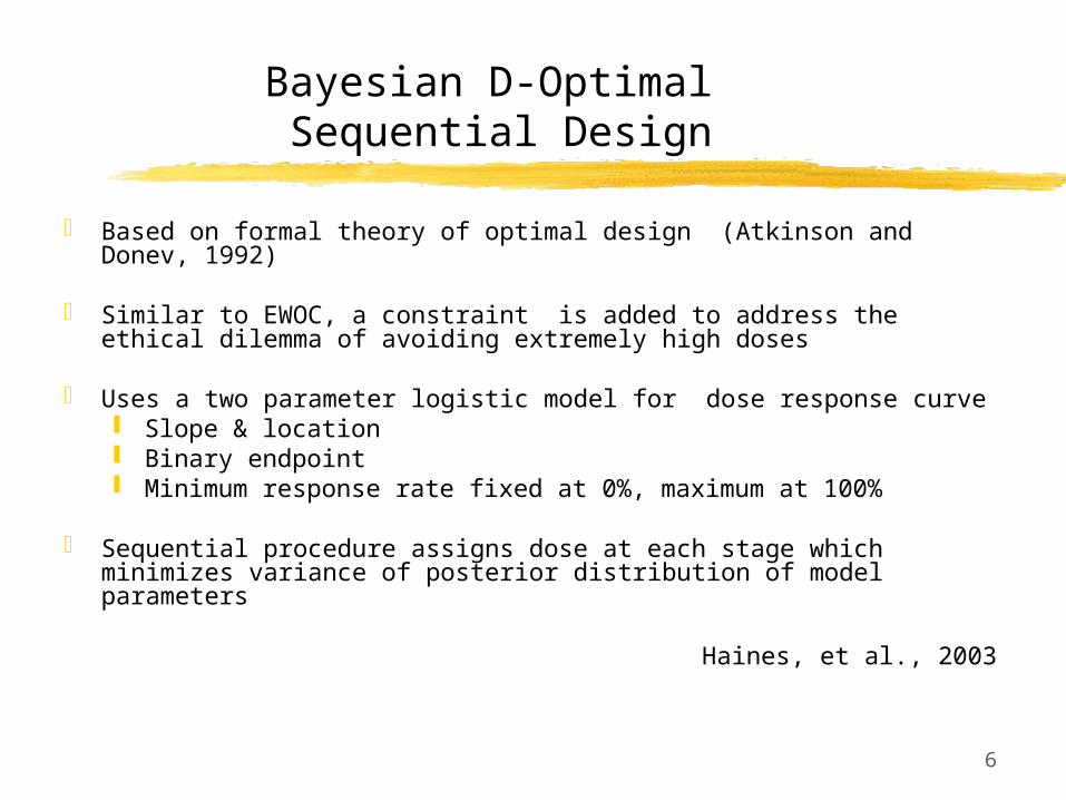
Bayesian D-Optimal Sequential Design
Based on formal theory of optimal design (Atkinson and Donev, 1992)
Similar to EWOC, a constraint is added to address the ethical dilemma of avoiding extremely high doses
Uses a two parameter logistic model for dose response curve Slope & location Binary endpoint Minimum response rate fixed at 0%, maximum at 100%
Sequential procedure assigns dose at each stage which minimizes variance of posterior distribution of model parameters
Haines, et al., 2003
7
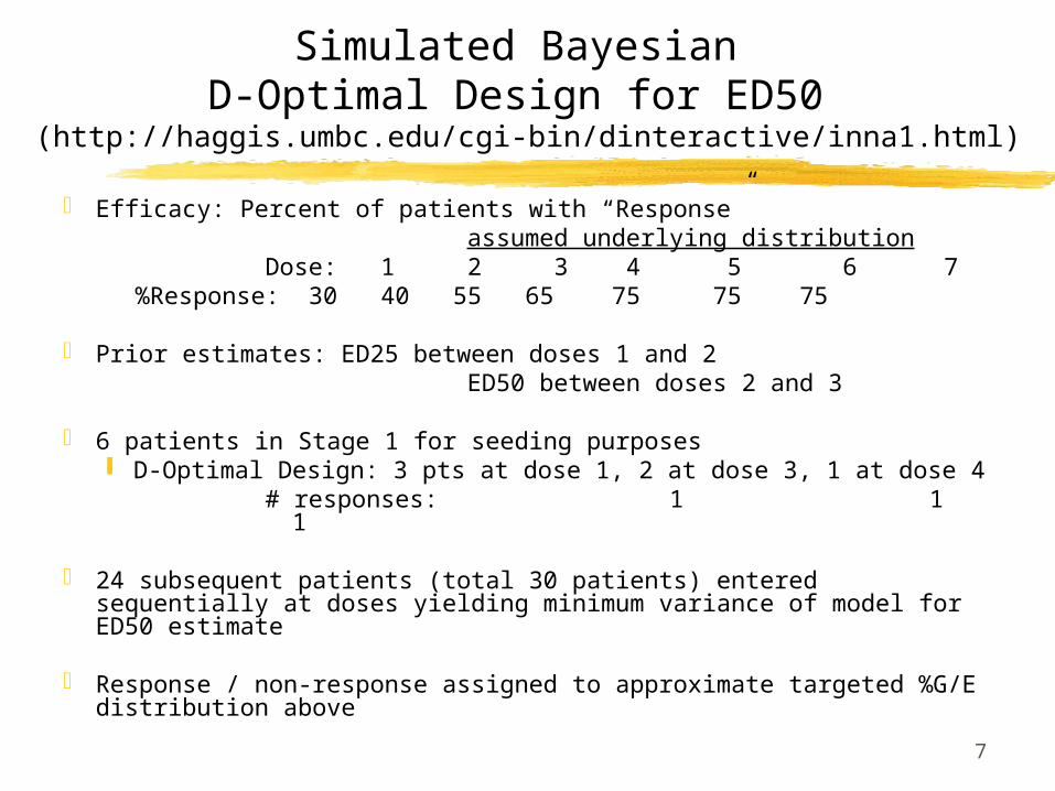
Simulated Bayesian D-Optimal Design for ED50
(http://haggis.umbc.edu/cgi-bin/dinteractive/inna1.html)
Efficacy: Percent of patients with “Response” assumed underlying distribution
Dose: 1 2 3 4 5 6 7 %Response: 30 40 55 65 75 75 75
Prior estimates: ED25 between doses 1 and 2 ED50 between doses 2 and 3
6 patients in Stage 1 for seeding purposes D-Optimal Design: 3 pts at dose 1, 2 at dose 3, 1 at dose 4 # responses: 1 1 1
24 subsequent patients (total 30 patients) entered sequentially at doses yielding minimum variance of model for ED50 estimate
Response / non-response assigned to approximate targeted %G/E distribution above
8
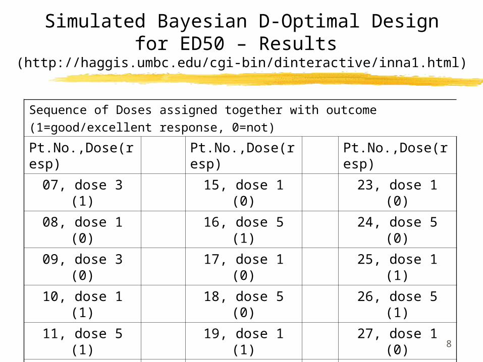
Simulated Bayesian D-Optimal Designfor ED50 – Results
(http://haggis.umbc.edu/cgi-bin/dinteractive/inna1.html)
Sequence of Doses assigned together with outcome(1=good/excellent response, 0=not)
Pt.No.,Dose(resp)
Pt.No.,Dose(resp)
Pt.No.,Dose(resp)
07, dose 3 (1) 15, dose 1 (0) 23, dose 1 (0)
08, dose 1 (0) 16, dose 5 (1) 24, dose 5 (0)
09, dose 3 (0) 17, dose 1 (0) 25, dose 1 (1)
10, dose 1 (1) 18, dose 5 (0) 26, dose 5 (1)
11, dose 5 (1) 19, dose 1 (1) 27, dose 1 (0)
12, dose 5 (0) 20, dose 5 (1) 28, dose 5 (0)
13, dsoe 5 (1) 21, dose 1 (0) 29, dose 1 (0)
14, dose 5 (1) 22, dose 5 (1) 30, dose 5 (1)
9
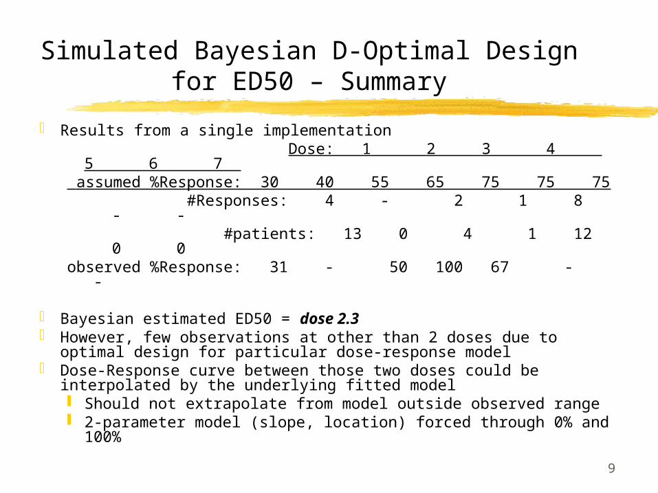
Simulated Bayesian D-Optimal Designfor ED50 – Summary
Results from a single implementation Dose: 1 2 3 4 5 6 7 assumed %Response: 30 40 55 65 75 75 75 #Responses: 4 - 2 1 8 - - #patients: 13 0 4 1 12 0 0observed %Response: 31 - 50 100 67 - -
Bayesian estimated ED50 = dose 2.3 However, few observations at other than 2 doses due to
optimal design for particular dose-response model Dose-Response curve between those two doses could be
interpolated by the underlying fitted model Should not extrapolate from model outside observed
range 2-parameter model (slope, location) forced through 0%
and 100%
10
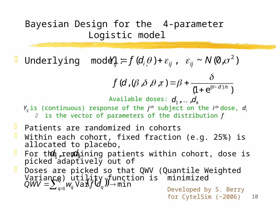
Bayesian Design for the 4-parameter Logistic model
Underlying model:
Available doses:
Yij is (continuous) response of the j-th subject on the i-th dose, di is the vector of parameters of the distribution f
Patients are randomized in cohorts Within each cohort, fixed fraction (e.g. 25%) is allocated to
placebo, For the remaining patients within cohort, dose is picked
adaptively out of Doses are picked so that QWV (Quantile Weighted Variance)
utility function is minimized
2,( ) , ~ (0, )ij i ij ijY f d N
( ) /( , ( , , , )
(1 e )df d
minVar1
Q
q qq dfwQWV
kdd ,,1
kdd ,,1
Developed by S. Berry for CytelSim (~2006)
11
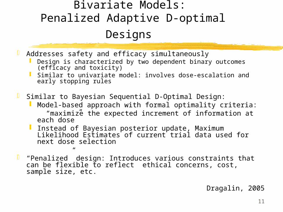
Bivariate Models:
Penalized Adaptive D-optimal Designs Addresses safety and efficacy simultaneously
Design is characterized by two dependent binary outcomes (efficacy and toxicity)
Similar to univariate model: involves dose-escalation and early stopping rules
Similar to Bayesian Sequential D-Optimal Design: Model-based approach with formal optimality criteria: “maximize the expected increment of information at
each dose” Instead of Bayesian posterior update, Maximum
Likelihood Estimates of current trial data used for next dose selection
“Penalized” design: Introduces various constraints that can be flexible to reflect ethical concerns, cost, sample size, etc.
Dragalin, 2005
12
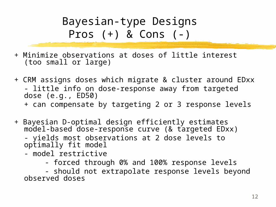
Bayesian-type DesignsPros (+) & Cons (-)
+ Minimize observations at doses of little interest (too small or large)
+ CRM assigns doses which migrate & cluster around EDxx- little info on dose-response away from targeted dose (e.g., ED50) + can compensate by targeting 2 or 3 response levels
+ Bayesian D-optimal design efficiently estimates model-based dose-response curve (& targeted EDxx)- yields most observations at 2 dose levels to optimally fit model- model restrictive
- forced through 0% and 100% response levels - should not extrapolate response levels beyond observed
doses
13
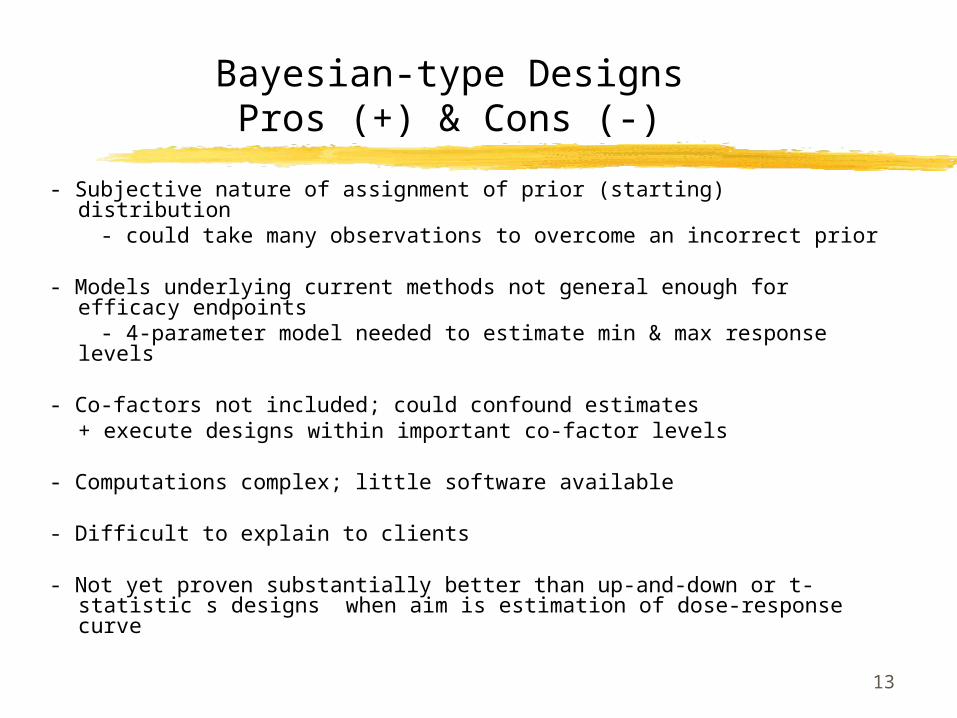
Bayesian-type DesignsPros (+) & Cons (-)
- Subjective nature of assignment of prior (starting) distribution - could take many observations to overcome an incorrect prior
- Models underlying current methods not general enough for efficacy endpoints
- 4-parameter model needed to estimate min & max response levels
- Co-factors not included; could confound estimates+ execute designs within important co-factor levels
- Computations complex; little software available
- Difficult to explain to clients
- Not yet proven substantially better than up-and-down or t-statistic s designs when aim is estimation of dose-response curve
14
Logistics for Conduct of a Dose-Adaptive Designed Trial
Response observable reasonably quickly
Increased statistical computations / simulations to justify dose-adaptive scheme in protocol
Need on-call person to assess previous response data and generate dose for next subject For model-based dose-adaptive designs, need on-call
unblinded statistician for associated analyses OR, this could be automated via web-based interface
(increases cost) Rapid transfer of needed data
Need special packaging or unblinded pharmacist at site to package selected dose for each patient
15
Remarks (2)
Logistics of implementation more complicated than usual parallel group design Frequent data calls / brief simple analyses Close contact with sites re: dose assignments Special packaging (IVRS??) Drug Supply – needed sufficiently for many possibilities
Tolerability rule(s) can be added for downward dose-assignment if pre-specified AE criteria are encountered This has been studied in context of Bayesian dose-
adaptive designs, but not in context of up&down designs Number of placebo patients maintained as designed for
intended precision vs. that group; could be down-sized, though
16
Dose-Adaptive DesignSummary
Allocation of dose for next subject based on response(s) of previous subject(s) Random Walk designs: only last subject’s response T-statistic (frequentist) designs: all previous subjects’
responses Bayesian-type designs: all previous subjects’ responses
High potential to limit subject allocation to doses of little interest (too high / too low) Maximize information gathered from fixed N Ethical advantage over fixed randomization More attractive to patients / subjects
Inference conditional on doses assigned by design, but not overly important in early development
Requires more statistical up-front work (simulation) No pre-specified allocation schedule; requires ongoing
communication with site regarding allocation
17
Dose-Adaptive Design Summary
Bayesian-type designs preferable to estimate dose-response curve; can also estimate a dose-response quantile of interest (e.g., EDxx) or (part of?) region of increasing dose-response Complex; heavy computations
Random Walk & T-statistic Designs focus on quantile(s) of interest Easy to understand & program Consider as starting point for implementing dose-
adaptive design Let other design features guide towards other adaptive
techniques based on particular experimental situation Ongoing incomplete simulations have yet to identify
major advantage of Bayesian-type designs over RW & T, unless prior information is important to consider.
Study, comparison, & refinement of these dose-adaptive designs continues
18
Dose-adaptive study designs offer benefits for proof-of-concept / Phase IIa clinical trials,
as well as raise issues for continued research
OUTLINE: Dose-Adaptive Designs & Examples Definition & Introduction (Jim) Frequentist Designs, including Random Walk Designs (Jim)
3+3 Design for cancer Up&Down Design Biased Coin Designs Simulations of Up&Down Design for Dental Pain Clinical Trial
Bayesian-type Designs (Inna) Continual Reassessment Method (CRM) Bayesian D-optimal Design Other related approaches Bayesian 4-parameter logistic
Case Study (Bayesian and Adaptive cross-over designs) CytelSim Software demo
Summary & Recommendations (Inna) References
Jim Bolognese & Inna Perevozskaya, Sept. 12, 2008
19
Case Study Example
Adaptive Dose-Ranging POC study
By I. Perevozskaya and Y. Tymofyeyev
20
Study Background
Development phase: Ib Strategic objective: generate preliminary D-R info to optimize
dose selection for Phase IIb study Caveats:
Phase Ib will be run using surrogate endpoint Future Phase IIb will be driven by clinical endpoint (chronic
symptoms) There is no formally established relationship between
surrogate and clinical endpoints dose-response curves, but… Dose selected as “sub-maximal” using surrogate endpoint D-R
curve is believed to be “sub-therapeutic” for the clinical endpoint.
21
Study objectives
(Broad) to demonstrate that a single administration of drug, compared with placebo, provides response that varies by dose
(Specific) 1. Find “sub-maximal” dose (e.g. ED75 defined as
the dose yielding 75% of the placebo-adjusted maximal response )
2. Meaningfully describe dose-response relationship
3. Demonstrate that at least one dose is significantly different from placebo
22
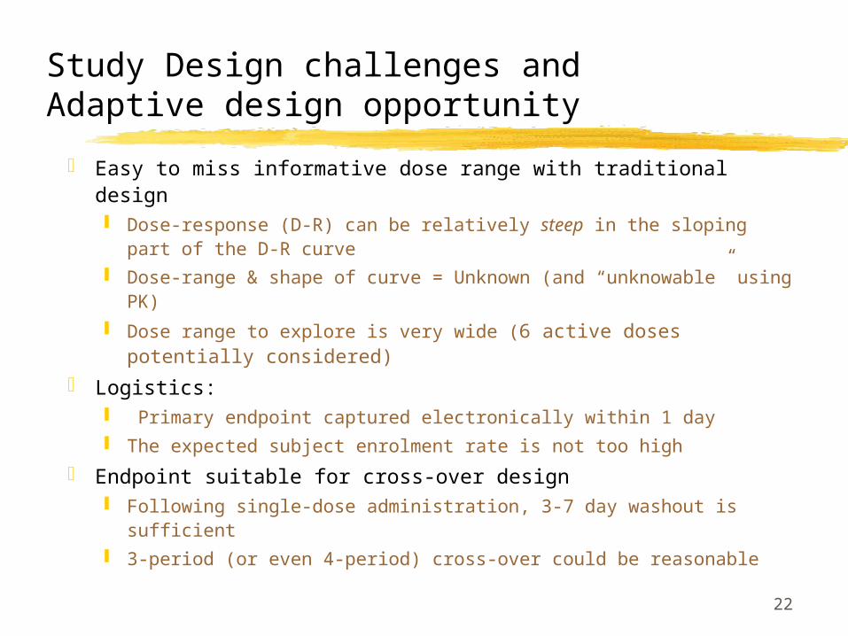
Study Design challenges and Adaptive design opportunity
Easy to miss informative dose range with traditional design Dose-response (D-R) can be relatively steep in the sloping part
of the D-R curve Dose-range & shape of curve = Unknown (and “unknowable”
using PK)
Dose range to explore is very wide (6 active doses potentially considered)
Logistics: Primary endpoint captured electronically within 1 day The expected subject enrolment rate is not too high
Endpoint suitable for cross-over design Following single-dose administration, 3-7 day washout is
sufficient 3-period (or even 4-period) cross-over could be reasonable
23
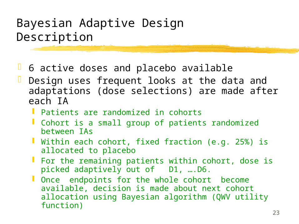
Bayesian Adaptive Design Description
6 active doses and placebo available Design uses frequent looks at the data and
adaptations (dose selections) are made after each IA Patients are randomized in cohorts Cohort is a small group of patients randomized between
IAs Within each cohort, fixed fraction (e.g. 25%) is allocated
to placebo For the remaining patients within cohort, dose is picked
adaptively out of D1, ….D6. Once endpoints for the whole cohort become available,
decision is made about next cohort allocation using Bayesian algorithm (QWV utility function)
24
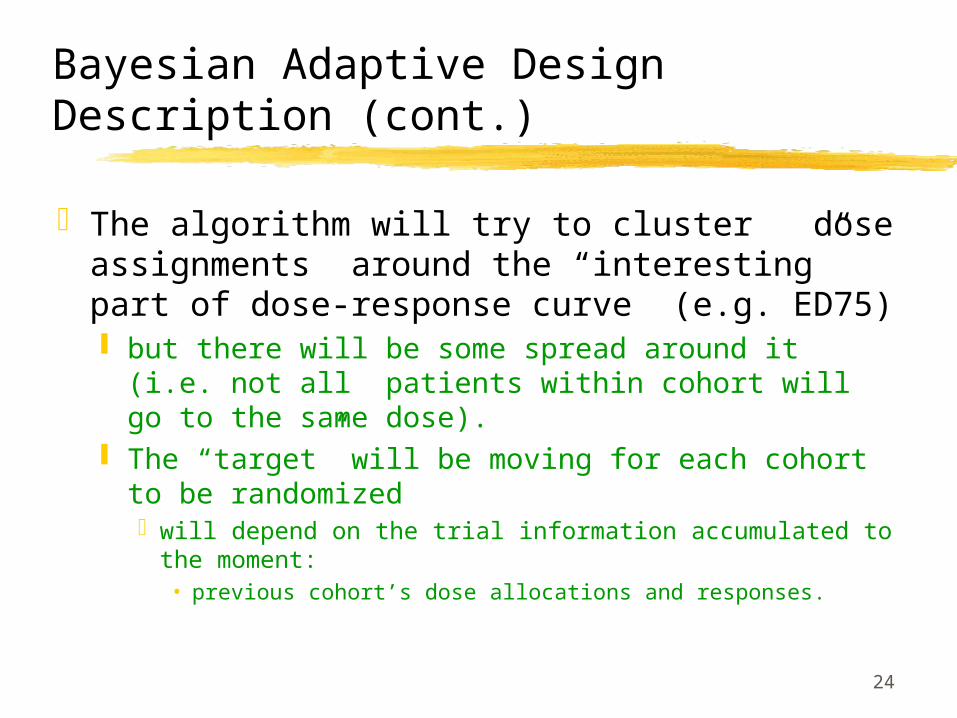
Bayesian Adaptive Design Description (cont.)
The algorithm will try to cluster dose assignments around the “interesting” part of dose-response curve (e.g. ED75) but there will be some spread around it (i.e. not
all patients within cohort will go to the same dose).
The “target” will be moving for each cohort to be randomized will depend on the trial information accumulated to the
moment: • previous cohort’s dose allocations and responses.
25
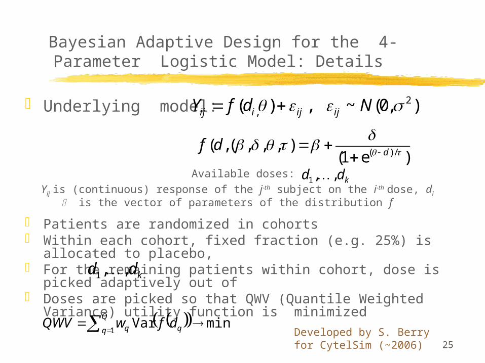
Bayesian Adaptive Design for the 4-Parameter Logistic Model: Details
Underlying model:
Available doses:
Yij is (continuous) response of the j-th subject on the i-th dose, di is the vector of parameters of the distribution f
Patients are randomized in cohorts Within each cohort, fixed fraction (e.g. 25%) is allocated to
placebo, For the remaining patients within cohort, dose is picked
adaptively out of Doses are picked so that QWV (Quantile Weighted Variance)
utility function is minimized
2,( ) , ~ (0, )ij i ij ijY f d N
( ) /( , ( , , , )
(1 e )df d
minVar1
Q
q qq dfwQWV
kdd ,,1
kdd ,,1
Developed by S. Berry for CytelSim (~2006)
26
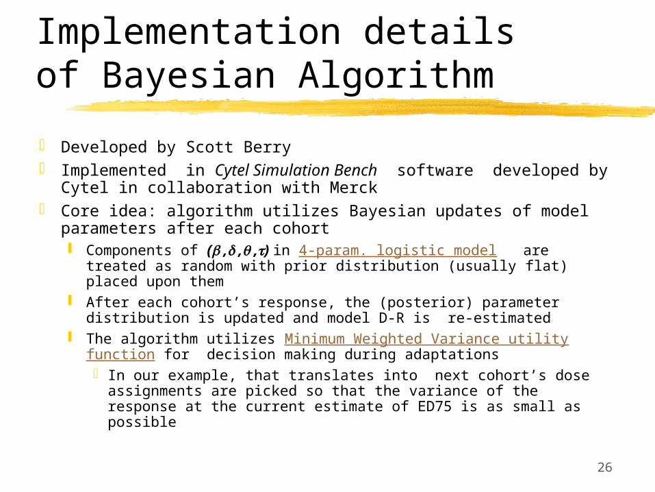
Implementation details of Bayesian Algorithm
Developed by Scott Berry Implemented in Cytel Simulation Bench software developed
by Cytel in collaboration with Merck Core idea: algorithm utilizes Bayesian updates of model
parameters after each cohort Components of ( , , ,) in 4-param. logistic model are
treated as random with prior distribution (usually flat) placed upon them
After each cohort’s response, the (posterior) parameter distribution is updated and model D-R is re-estimated
The algorithm utilizes Minimum Weighted Variance utility function for decision making during adaptations In our example, that translates into next cohort’s dose
assignments are picked so that the variance of the response at the current estimate of ED75 is as small as possible
27
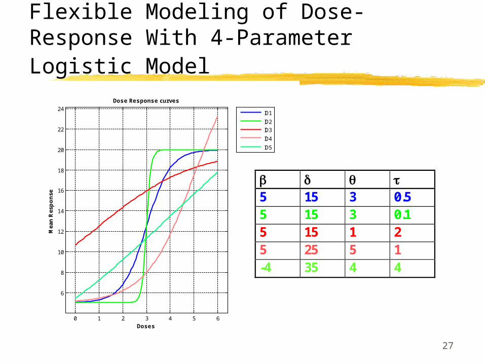
Flexible Modeling of Dose-Response With 4-Parameter Logistic Model
0 1 2 3 4 5 6
6
8
10
12
14
16
18
20
22
24
Doses
Mea
n R
esp
on
se
Dose Response curves
ID1
ID2
ID3
ID4
ID5
5 15 3 0.5 5 15 3 0.1 5 15 1 2 5 25 5 1 -4 35 4 4
28
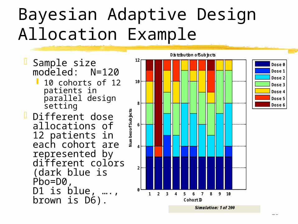
Bayesian Adaptive Design Allocation Example
1 2 3 4 5 6 7 8 9 100
2
4
6
8
10
12
Cohort ID
Nu
mb
er o
f S
ub
ject
s
Distribution ofSubjects
Dose 0
Dose 1
Dose 2
Dose 3
Dose 4
Dose 5
Dose 6
Sample size modeled: N=120 10 cohorts of 12
patients in parallel design setting
Different dose allocations of 12 patients in each cohort are represented by different colors (dark blue is Pbo=D0, D1 is blue, …., brown is D6).
29
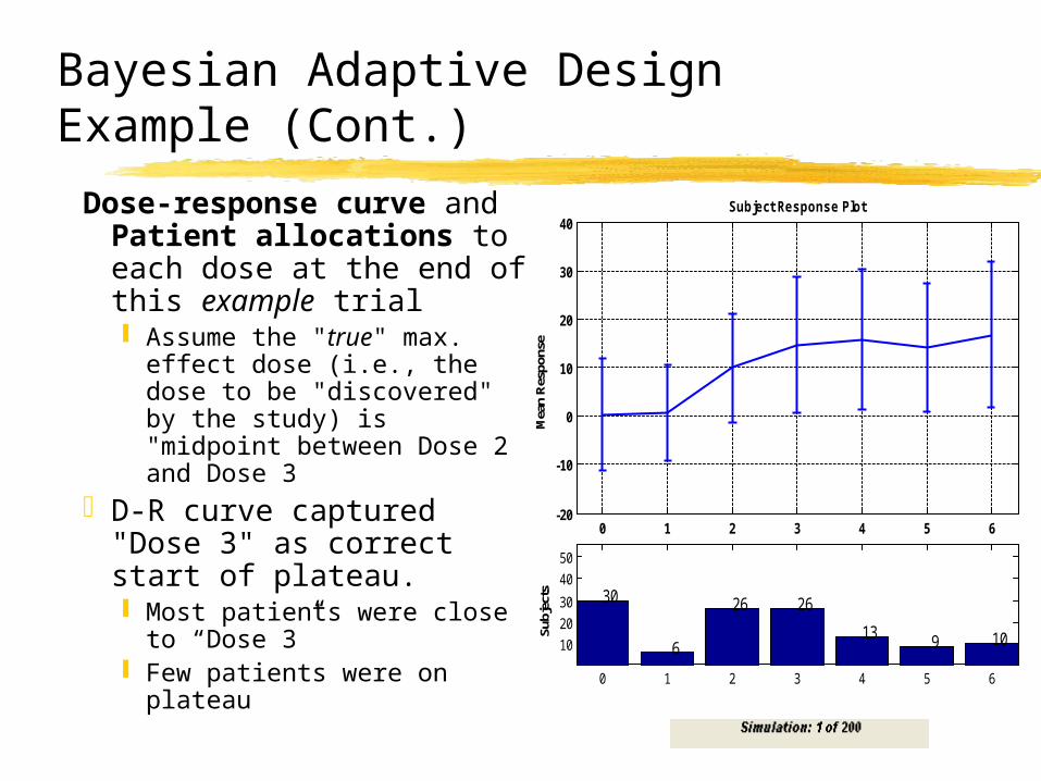
Bayesian Adaptive Design Example (Cont.)
0 1 2 3 4 5 6-20
-10
0
10
20
30
40
Mea
n R
espo
nse
Subject Response Plot
0 1 2 3 4 5 6
10
20
30
40
50
30
6
26 26
13 9 10Subj
ects
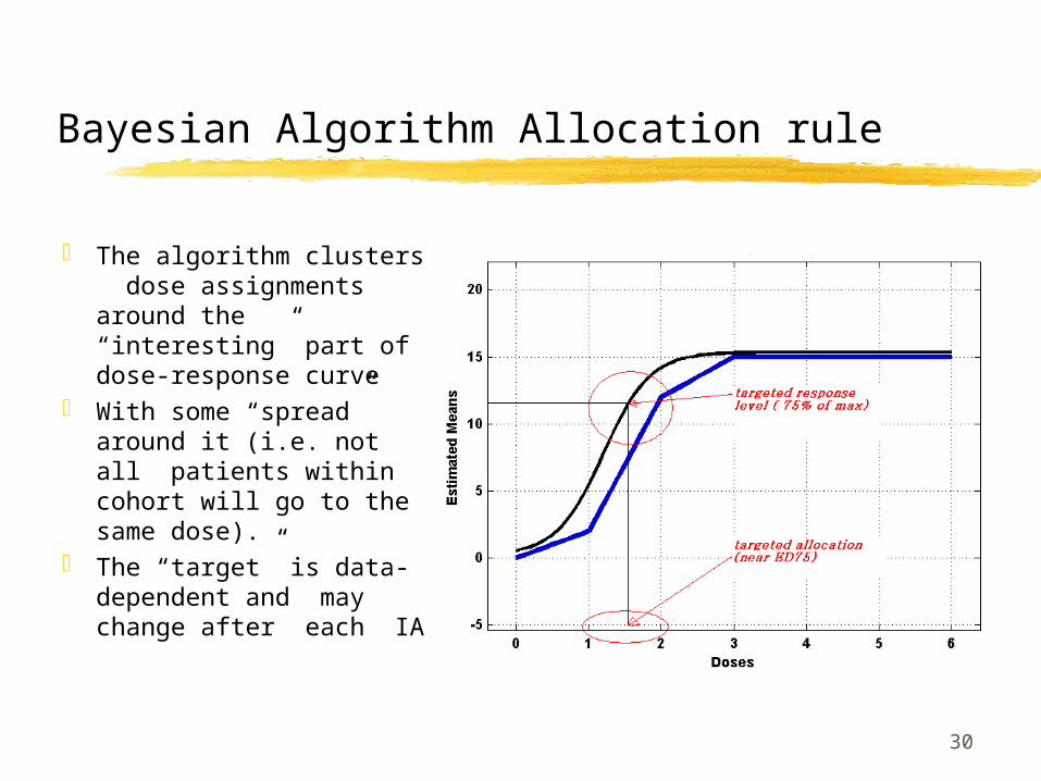
Dose-response curve and Patient allocations to each dose at the end of this example trial Assume the "true" max.
effect dose (i.e., the dose to be "discovered" by the study) is "midpoint between Dose 2 and Dose 3
D-R curve captured "Dose 3" as correct start of plateau. Most patients were close to
“Dose 3” Few patients were on
plateau
30
Bayesian Algorithm Allocation rule
The algorithm clusters dose assignments around the “interesting” part of dose-response curve
With some “spread” around it (i.e. not all patients within cohort will go to the same dose).
The “target” is data-dependent and may change after each IA
31
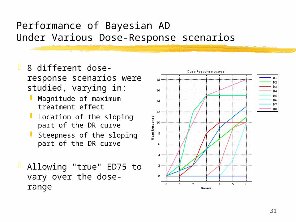
Performance of Bayesian AD Under Various Dose-Response scenarios
8 different dose-response scenarios were studied, varying in: Magnitude of maximum
treatment effect Location of the sloping part
of the DR curve Steepness of the sloping
part of the DR curve
Allowing "true" ED75 to vary over the dose-range 0 1 2 3 4 5 6
0
2
4
6
8
10
12
14
16
18
Doses
Me
an
Re
sp
on
se
Dose Response curves
ID1
ID2
ID3
ID4
ID5
ID6
ID7
ID8
32
Performance of Bayesian AD Under Various Dose-Response scenarios (cont.)
Performance evaluated via simulations (using CytelSim Software)
Key criteria for evaluation included1. Subject allocation pattern2. Precision of picking “right dose” correctly3. Power and Type I error for detecting dose-
response 4. Precision of overall D-R estimation across all
doses (measured by MSE)
33
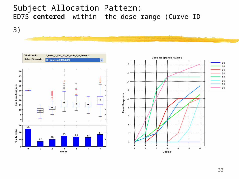
Subject Allocation Pattern:
ED75 centered within the dose range (Curve ID 3)
0
5
10
15
20
25
30
35
40
45
50
Nu
mb
er
of
su
bje
cts
0 1 2 3 4 5 60
10
20
3025
7.210
15 13 1317
Doses
% A
llo
ca
tio
n
0 1 2 3 4 5 6
0
2
4
6
8
10
12
14
16
18
Doses
Me
an
Re
sp
on
se
Dose Response curves
ID1
ID2
ID3
ID4
ID5
ID6
ID7
ID8
34
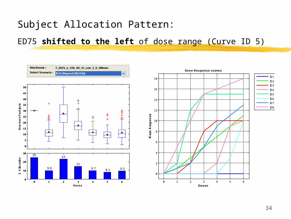
Subject Allocation Pattern:
ED75 shifted to the left of dose range (Curve ID 5)
0 1 2 3 4 5 6
0
2
4
6
8
10
12
14
16
18
Doses
Me
an
Re
sp
on
se
Dose Response curves
ID1
ID2
ID3
ID4
ID5
ID6
ID7
ID8
0
5
10
15
20
25
30
35
40
45
50
Nu
mb
er
of
su
bje
cts
0 1 2 3 4 5 60
10
20
3025
9.9
23
159.7 8.1 9.5
Doses
% A
llo
ca
tio
n
35
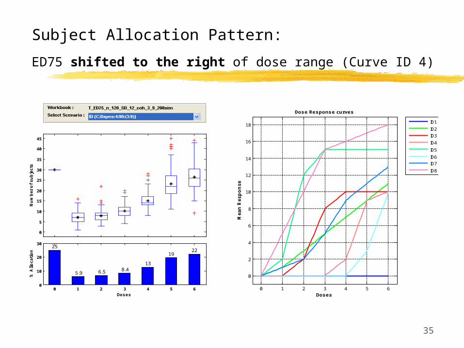
Subject Allocation Pattern:
ED75 shifted to the right of dose range (Curve ID 4)
0 1 2 3 4 5 6
0
2
4
6
8
10
12
14
16
18
Doses
Me
an
Re
sp
on
se
Dose Response curves
ID1
ID2
ID3
ID4
ID5
ID6
ID7
ID8
0
5
10
15
20
25
30
35
40
45
Nu
mb
er
of
su
bje
cts
0 1 2 3 4 5 60
10
20
3025
5.9 6.5 8.413
1922
Doses
% A
llo
ca
tio
n
36
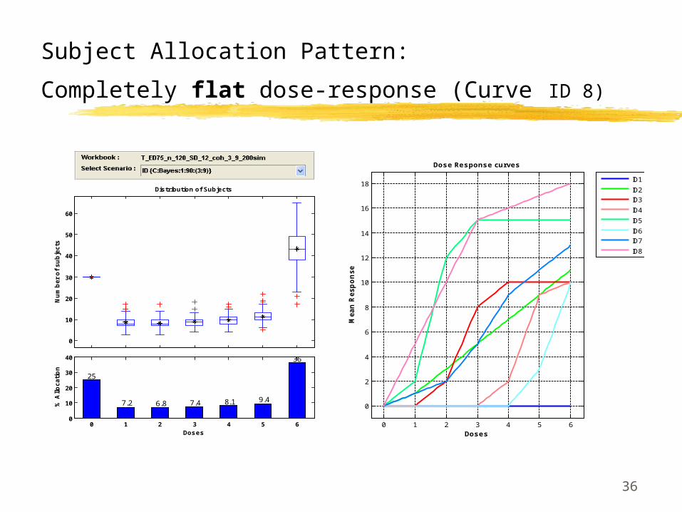
Subject Allocation Pattern:
Completely flat dose-response (Curve ID 8)
0 1 2 3 4 5 6
0
2
4
6
8
10
12
14
16
18
Doses
Me
an
Re
sp
on
se
Dose Response curves
ID1
ID2
ID3
ID4
ID5
ID6
ID7
ID8
0
10
20
30
40
50
60
Nu
mb
er
of
su
bje
cts
Distribution of Subjects
0 1 2 3 4 5 60
10
20
30
40
25
7.2 6.8 7.4 8.1 9.4
36
Doses
% A
llo
ca
tio
n
37
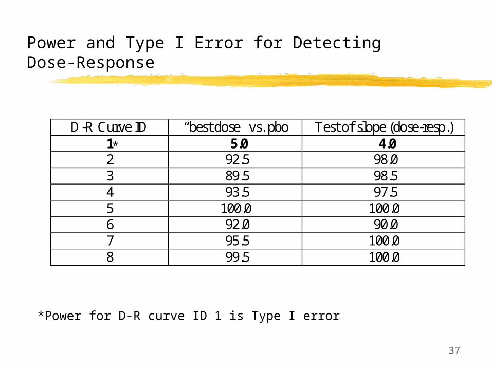
Power and Type I Error for Detecting Dose-Response
D-R Curve ID “best dose” vs. pbo Test of slope (dose-resp.) 1 5.0 4.0 2 92.5 98.0 3 89.5 98.5 4 93.5 97.5 5 100.0 100.0 6 92.0 90.0 7 95.5 100.0 8 99.5 100.0
*Power for D-R curve ID 1 is Type I error
*
38
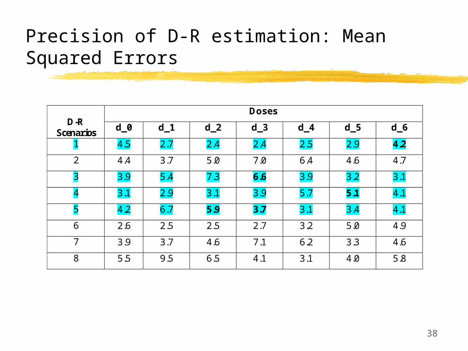
Precision of D-R estimation: Mean Squared Errors
Doses D-R
Scenarios d_0 d_1 d_2 d_3 d_4 d_5 d_6
1 4.5 2.7 2.4 2.4 2.5 2.9 4.2
2 4.4 3.7 5.0 7.0 6.4 4.6 4.7
3 3.9 5.4 7.3 6.6 3.9 3.2 3.1
4 3.1 2.9 3.1 3.9 5.7 5.1 4.1
5 4.2 6.7 5.9 3.7 3.1 3.4 4.1
6 2.6 2.5 2.5 2.7 3.2 5.0 4.9
7 3.9 3.7 4.6 7.1 6.2 3.3 4.6
8 5.5 9.5 6.5 4.1 3.1 4.0 5.8
39
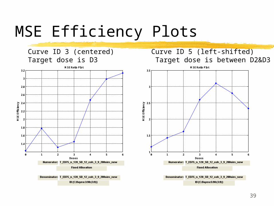
MSE Efficiency Plots
0 1 2 3 4 5 6
1.4
1.6
1.8
2
2.2
2.4
2.6
2.8
3
3.2
Doses
MS
E E
ffic
ien
cy
MSE Ratio Plot
0 1 2 3 4 5 61
1.5
2
2.5
3
3.5
Doses
MS
E E
ffic
ien
cy
MSE Ratio Plot
Curve ID 3 (centered) Target dose is D3
Curve ID 5 (left-shifted) Target dose is between D2&D3
40
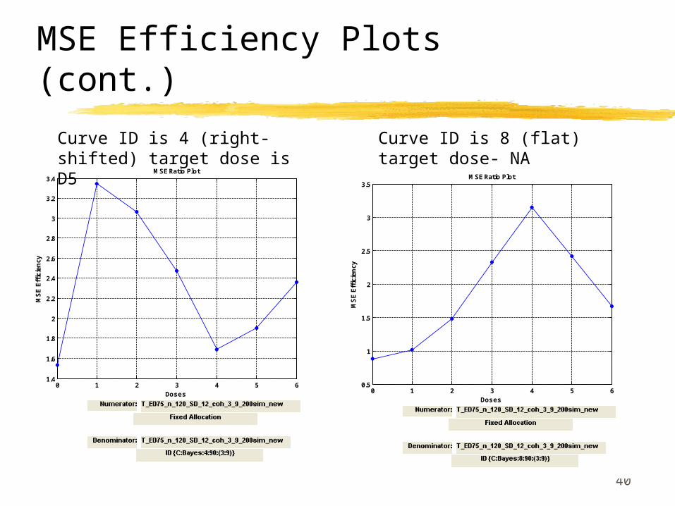
MSE Efficiency Plots (cont.)
0 1 2 3 4 5 61.4
1.6
1.8
2
2.2
2.4
2.6
2.8
3
3.2
3.4
Doses
MS
E E
ffic
ien
cy
MSE Ratio Plot
0 1 2 3 4 5 60.5
1
1.5
2
2.5
3
3.5
Doses
MS
E E
ffic
ien
cy
MSE Ratio Plot
Curve ID is 4 (right-shifted) target dose is D5
Curve ID is 8 (flat) target dose- NA
41
Summary of Bayesian Design Simulations
In all 7 non-flat D-R scenarios, the design maximized allocations around the “true” ED75.
In case of flat D-R, most patients were allocated to max dose and placebo with very little in between
Type I error was preserved Power to detect a dose-response is at least 90% Power to detect a significant difference between the best
dose and placebo is at least 89.5% For all scenarios, AD design was uniformly more efficient
than fixed design of the same sample size (measured by MSE ratio across doses )
42
Further Steps
Simulations have shown that Bayesian AD design may adequately address the Ib study objectives: A definitive single dose for Phase III was NOT needed General idea about D-R needed: upper/lower plateau,
sloping part
Due to absence of readily available software for crossover design, these computer simulations used N=120 in a parallel design setting It was anticipated that similar results for power and
Type 1 error could be obtained using N=30 subjects each contributing 4 measurements
43
Further Steps (cont.)
Crossover-like framework preferable to parallel design framework between/within subject variability => sample size
considerations ( 30 vs. 120) short drug half-life -> short washout period
Option 1: modify Bayesian design so that each subject can contribute multiple measurements incorporate repeated-measures in modeling and simulations Required involvement of external vendor and extra time to
complete both simulator and randomizer Option 2: consider true crossover design but change doses
adaptively Non-Bayesian approach Could be accomplished in-house within approximately the same
timeframe due to lower computational complexity Can be reduced to “standard” crossover if no dose adjustment
takes place
44
Adaptive Crossover Design Highlights
Doses explored: {D1, …, D6} of Merck-X + pbo Based on: 4 period crossover
Pbo + active doses A,B,C Values of A, B, C are subset of {D1, …, D6} and change
dynamically after each interim look (~twice weekly) Time-to-endpoint + washout is 1 week
Decision rule: pick a subset of doses {A, B, C} from {D1, …, D6} based on (non-Bayesian) utility function
Utility function: cumulative score describing proximity of each dose to target ED75 according to current estimate of D-R
D-R estimation: based on isotonic regression model
45
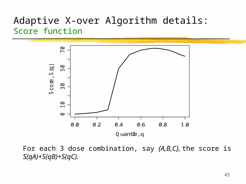
Adaptive X-over Algorithm details: Score function
0.0 0.2 0.4 0.6 0.8 1.0
01
03
05
07
0
Quantile, q
Sco
re, S
(q)
For each 3 dose combination, say {A,B,C}, the score is S(qA)+S(qB)+S(qC).
46
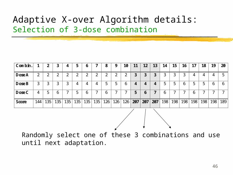
Adaptive X-over Algorithm details: Selection of 3-dose combination
Combin. 1 2 3 4 5 6 7 8 9 10 11 12 13 14 15 16 17 18 19 20
Dose A 2 2 2 2 2 2 2 2 2 2 3 3 3 3 3 3 4 4 4 5
Dose B 3 3 3 3 4 4 4 5 5 6 4 4 4 5 5 6 5 5 6 6
Dose C 4 5 6 7 5 6 7 6 7 7 5 6 7 6 7 7 6 7 7 7
Score 144 135 135 135 135 135 135 126 126 126 207 207 207 198 198 198 198 198 198 189
Randomly select one of these 3 combinations and use until next adaptation.
47
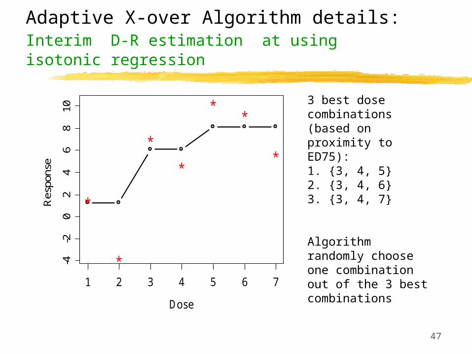
Adaptive X-over Algorithm details: Interim D-R estimation at using isotonic regression
1 2 3 4 5 6 7
-4-2
02
46
810
Dose
Res
pons
e
*
*
*
*
**
*
3 best dose combinations (based on proximity to ED75):1. {3, 4, 5}2. {3, 4, 6}3. {3, 4, 7}
Algorithm randomly choose one combination out of the 3 best combinations
48
Adaptive Cross-Over Design Performance
Characteristics via Simulations Several D-R scenarios were explored Allocation pattern:
similar to Bayesian design, the algorithm allocates subjects to the neighborhood of the effective and the highest sub-effective dose levels
N=60 patients adequate to achieve ~80% or better power for “best dose” vs. placebo comparison Type I error is preserved
Caveat: effect sizes were smaller than those explored for Bayesian AD This contributed to sample size increase from N=30 (30 patients*4
obs.=120obs) for Bayesian AD to N=60 (60 patients*4 obs. =240 obs.) for the adaptive crossover design
49Dose
Re
spo
nse
0
2
4
6
8Scenario 1
1 2 3 4 5 6 7
Scenario 2 Scenario 3
Scenario 4 Scenario 5
0
2
4
6
8Scenario 6
0
2
4
6
8Scenario 7 Scenario 8 Scenario 9
1 2 3 4 5 6 7
Scenario 10 Scenario 11
1 2 3 4 5 6 7
0
2
4
6
8Scenario 12
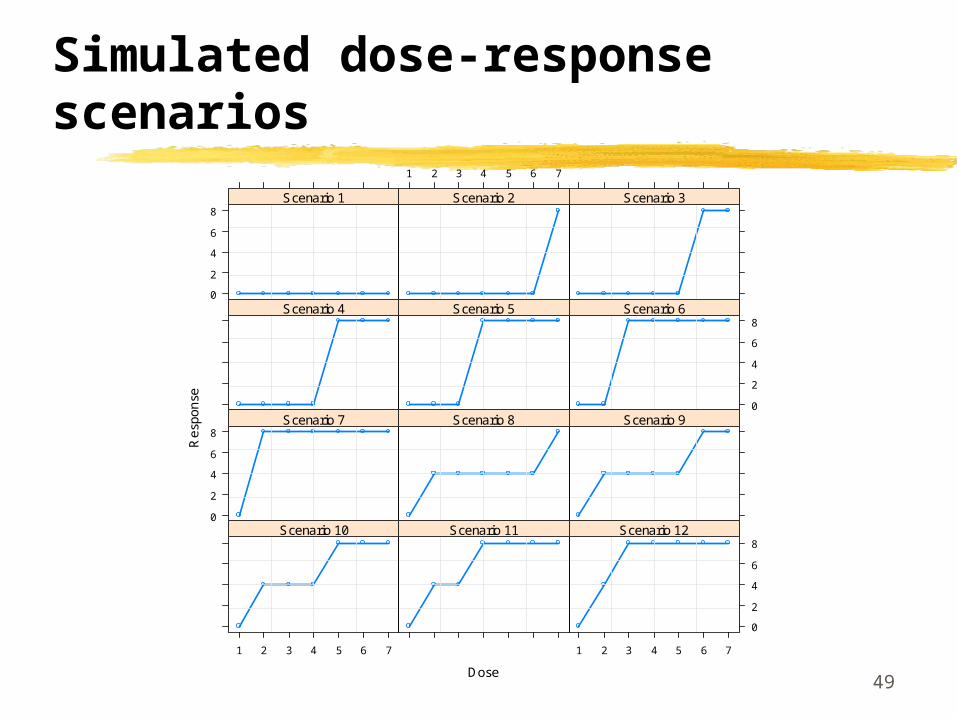
Simulated dose-response scenarios
50
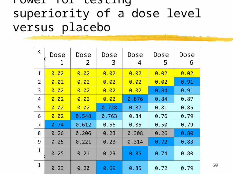
Power for testing superiority of a dose level versus placebo
Sc. Dose 1 Dose 2 Dose 3 Dose 4 Dose 5 Dose 6
1 0.02 0.02 0.02 0.02 0.02 0.02
2 0.02 0.02 0.02 0.02 0.02 0.91
3 0.02 0.02 0.02 0.02 0.84 0.91
4 0.02 0.02 0.02 0.876 0.84 0.87
5 0.02 0.02 0.728 0.87 0.81 0.85
6 0.02 0.548 0.763 0.84 0.76 0.79
7 0.74 0.612 0.56 0.85 0.50 0.79
8 0.26 0.206 0.23 0.308 0.26 0.80
9 0.25 0.221 0.23 0.314 0.72 0.83
10 0.25 0.21 0.23 0.85 0.74 0.80
11 0.23 0.20 0.69 0.85 0.72 0.79
12 0.22 0.62 0.70 0.84 0.69 0.75
51
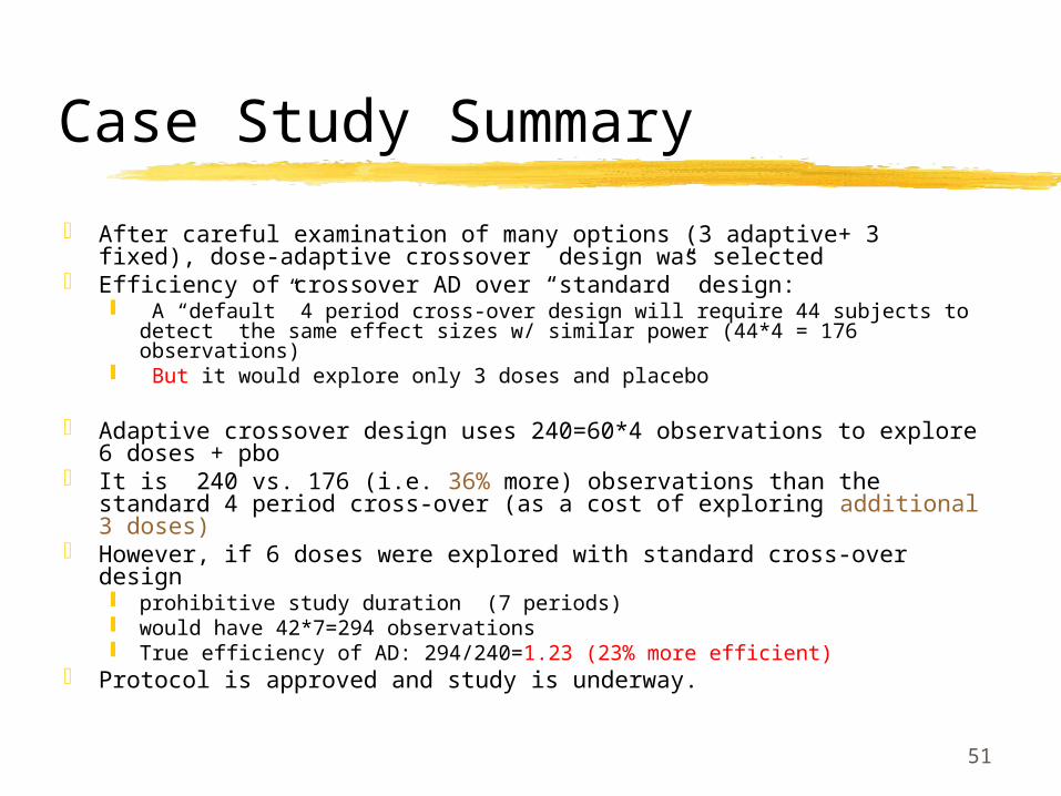
Case Study Summary
After careful examination of many options (3 adaptive+ 3 fixed), dose-adaptive crossover design was selected
Efficiency of crossover AD over “standard” design: A “default” 4 period cross-over design will require 44 subjects to detect
the same effect sizes w/ similar power (44*4 = 176 observations) But it would explore only 3 doses and placebo
Adaptive crossover design uses 240=60*4 observations to explore 6 doses + pbo
It is 240 vs. 176 (i.e. 36% more) observations than the standard 4 period cross-over (as a cost of exploring additional 3 doses)
However, if 6 doses were explored with standard cross-over design prohibitive study duration (7 periods) would have 42*7=294 observations True efficiency of AD: 294/240=1.23 (23% more efficient)
Protocol is approved and study is underway.
52
Dose-adaptive study designs offer benefits for proof-of-concept / Phase IIa clinical trials,
as well as raise issues for continued research
OUTLINE: Dose-Adaptive Designs & Examples Definition & Introduction (Jim) Frequentist Designs, including Random Walk Designs (Jim)
3+3 Design for cancer Up&Down Design Biased Coin Designs Simulations of Up&Down Design for Dental Pain Clinical Trial
Bayesian-type Designs (Inna) Continual Reassessment Method (CRM) Bayesian D-optimal Design Other related approaches Bayesian 4-parameter logistic
Case Study (Bayesian and Adaptive cross-over designs) CytelSim Software demo
Summary & Recommendations (Inna) References
Jim Bolognese & Inna Perevozskaya, Sept. 12, 2008
53
Cytel Simulation Bench (CytelSim) Software for adaptive designs: Background and History
Developed by Cytel Statistical Software in collaboration with Merck Team
Currently exists as an in-house tool Production version planned for near future Merck (BARDS) development team:
Jim Bolognese Inna Perevozskaya Yevgen Tymofyeyev Jason Clark
54
Cytel Simulation Bench (CytelSim) Software for adaptive designs: Background and History (cont.)
Focus: model – based designs for early stage adaptive dose-ranging studies with multiple IAs
Development started shortly after 1st BARDS AD grand rounds in July 2005 Rationale for development: surging interest in innovative
design methodologies for dose-ranging studies Simulations are crucial step for implementation of such
designs Original goal: to compare performances of a Bayesian design
and up-and-down (Frequentist) design on the same platform Other methods and more sophisticated interface added later
as project needs grew
This project is still work–in-progress
55
CytelSim Underlying Methodology Overview
Applicable to early stage adaptive dose-ranging studies Provides simulations for model-based design and analysis
for such studies General set-up:
Doses of the drug and of the placebo are available for administration
Subjects are enrolled and treated in groups, known as cohorts. The size and composition of each cohort can be user-specified
and may include a fixed number of subjects assigned to placebo
Active control arm may be included as well
kdd ,,1 0d
56
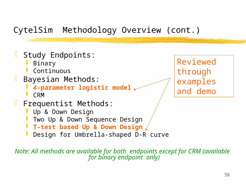
CytelSim Methodology Overview (cont.)
Study Endpoints: Binary Continuous
Bayesian Methods: 4-parameter logistic model CRM
Frequentist Methods: Up & Down Design Two Up & Down Sequence Design T-test based Up & Down Design Design for Umbrella-shaped D-R curve
Note: All methods are available for both endpoints except for CRM (available for binary endpoint only)
Reviewed through examples and demo
57
T-statistic methodology highlights
Frequentist method designed to cluster allocations around target dose of interest
Can be ran for 1 or 2 targets Target is defined as difference from placebo in response or
an absolute value of response variable After each IA, T-test Based Up&Down Design assigns all
subjects in a next cohort to a single dose Dose chosen by comparing a t-statistic (based on all
previous responses at a dose) to a set of user-defined dose escalation rules: -2, -1, 0, +1, and +2 doses
More details in Example 1.Note: differences from Bayesian design are highlighted
58
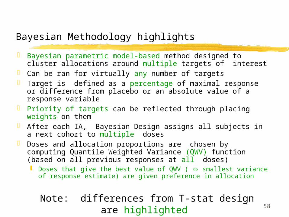
Bayesian Methodology highlights
Bayesian parametric model-based method designed to cluster allocations around multiple targets of interest
Can be ran for virtually any number of targets Target is defined as a percentage of maximal response or
difference from placebo or an absolute value of a response variable
Priority of targets can be reflected through placing weights on them
After each IA, Bayesian Design assigns all subjects in a next cohort to multiple doses
Doses and allocation proportions are chosen by computing Quantile Weighted Variance (QWV) function (based on all previous responses at all doses) Doses that give the best value of QWV ( smallest variance of
response estimate) are given preference in allocation
Note: differences from T-stat design are highlighted
60
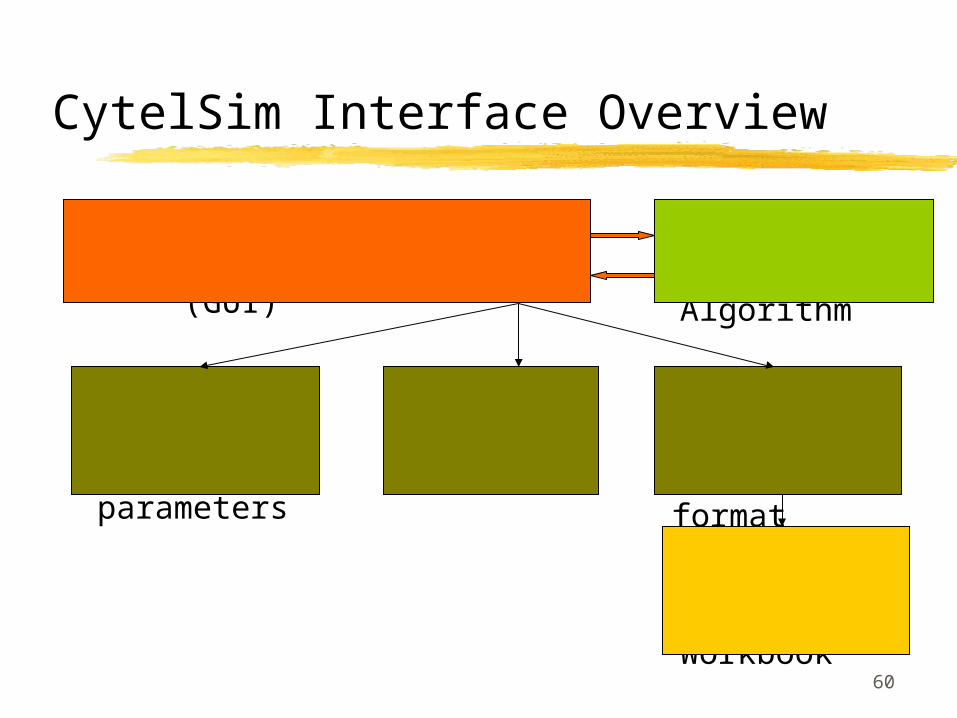
CytelSim Interface Overview
User Interface (GUI)
Computational Algorithm
Input and store simulation parameters
Output file in tabular format
Graphic summaries
Export to Excel Workbook
61
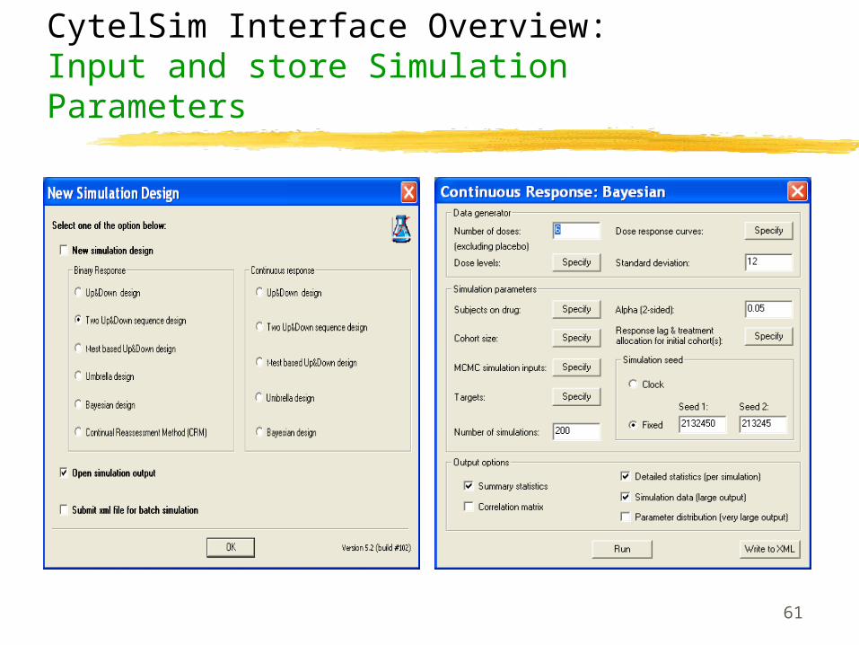
CytelSim Interface Overview:Input and store Simulation Parameters
62
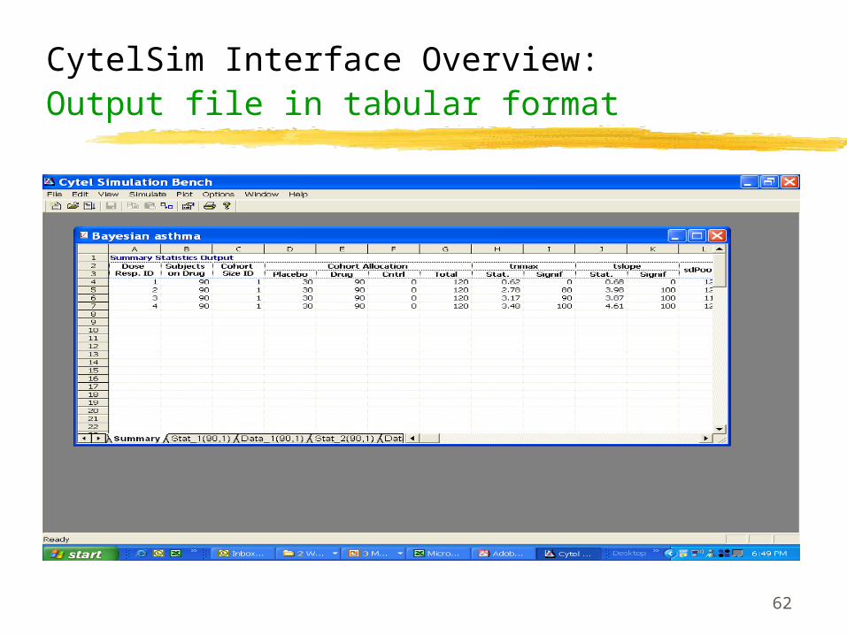
CytelSim Interface Overview:Output file in tabular format
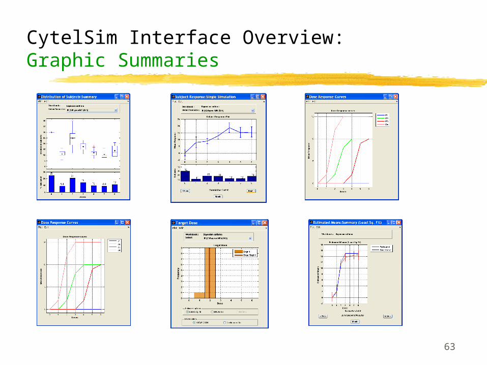
63
CytelSim Interface Overview:Graphic Summaries
64
CytelSim Software Demo:
Simulating Bayesian Design
Cytel Simulation Bench
65
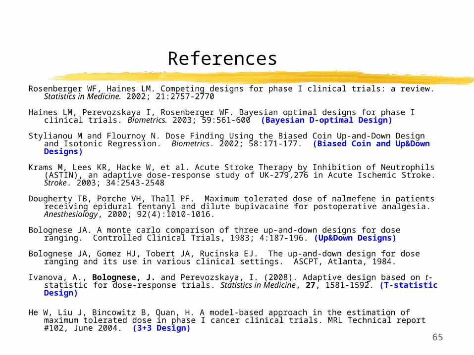
References
Rosenberger WF, Haines LM. Competing designs for phase I clinical trials: a review. Statistics in Medicine. 2002; 21:2757-2770
Haines LM, Perevozskaya I, Rosenberger WF. Bayesian optimal designs for phase I clinical trials. Biometrics. 2003; 59:561-600 (Bayesian D-optimal Design)
Stylianou M and Flournoy N. Dose Finding Using the Biased Coin Up-and-Down Design and Isotonic Regression. Biometrics. 2002; 58:171-177. (Biased Coin and Up&Down Designs)
Krams M, Lees KR, Hacke W, et al. Acute Stroke Therapy by Inhibition of Neutrophils (ASTIN), an adaptive dose-response study of UK-279,276 in Acute Ischemic Stroke. Stroke. 2003; 34:2543-2548
Dougherty TB, Porche VH, Thall PF. Maximum tolerated dose of nalmefene in patients receiving epidural fentanyl and dilute bupivacaine for postoperative analgesia. Anesthesiology, 2000; 92(4):1010-1016.
Bolognese JA. A monte carlo comparison of three up-and-down designs for dose ranging. Controlled Clinical Trials, 1983; 4:187-196. (Up&Down Designs)
Bolognese JA, Gomez HJ, Tobert JA, Rucinska EJ. The up-and-down design for dose ranging and its use in various clinical settings. ASCPT, Atlanta, 1984.
Ivanova, A., Bolognese, J. and Perevozskaya, I. (2008). Adaptive design based on t-statistic for dose-response trials. Statistics in Medicine, 27, 1581-1592. (T-statistic Design)
He W, Liu J, Bincowitz B, Quan, H. A model-based approach in the estimation of maximum tolerated dose in phase I cancer clinical trials. MRL Technical report #102, June 2004. (3+3 Design)
66
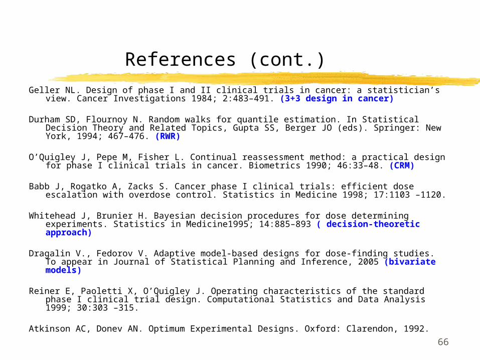
References (cont.)
Geller NL. Design of phase I and II clinical trials in cancer: a statistician’s view. Cancer Investigations 1984; 2:483–491. (3+3 design in cancer)
Durham SD, Flournoy N. Random walks for quantile estimation. In Statistical Decision Theory and Related Topics, Gupta SS, Berger JO (eds). Springer: New York, 1994; 467–476. (RWR)
O’Quigley J, Pepe M, Fisher L. Continual reassessment method: a practical design for phase I clinical trials in cancer. Biometrics 1990; 46:33–48. (CRM)
Babb J, Rogatko A, Zacks S. Cancer phase I clinical trials: efficient dose escalation with overdose control. Statistics in Medicine 1998; 17:1103 –1120.
Whitehead J, Brunier H. Bayesian decision procedures for dose determining experiments. Statistics in Medicine1995; 14:885–893 ( decision-theoretic approach)
Dragalin V., Fedorov V. Adaptive model-based designs for dose-finding studies. To appear in Journal of Statistical Planning and Inference, 2005 (bivariate models)
Reiner E, Paoletti X, O’Quigley J. Operating characteristics of the standard phase I clinical trial design. Computational Statistics and Data Analysis 1999; 30:303 –315.
Atkinson AC, Donev AN. Optimum Experimental Designs. Oxford: Clarendon, 1992.
67
QUESTIONS/ COMMENTS
/ DISCUSSION
Dose-adaptive study designs offer benefits for proof-of-concept / Phase IIa clinical trials,
as well as raise issues for continued research
68
Backups
Additional example of Bayesian Design: ASTIN trial
Select Simulation results for adaptive crossover design
69
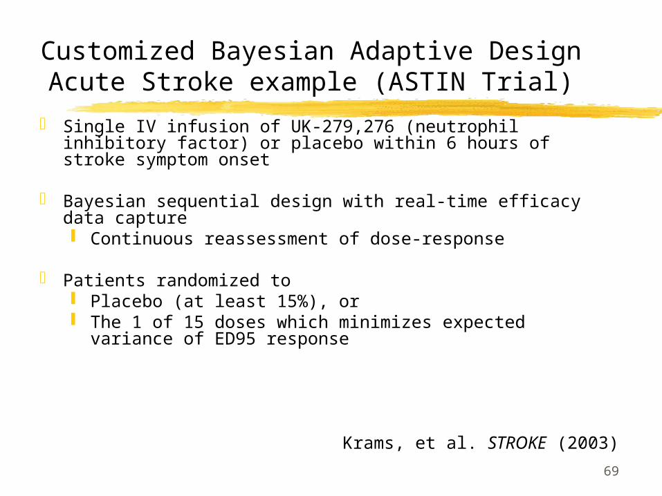
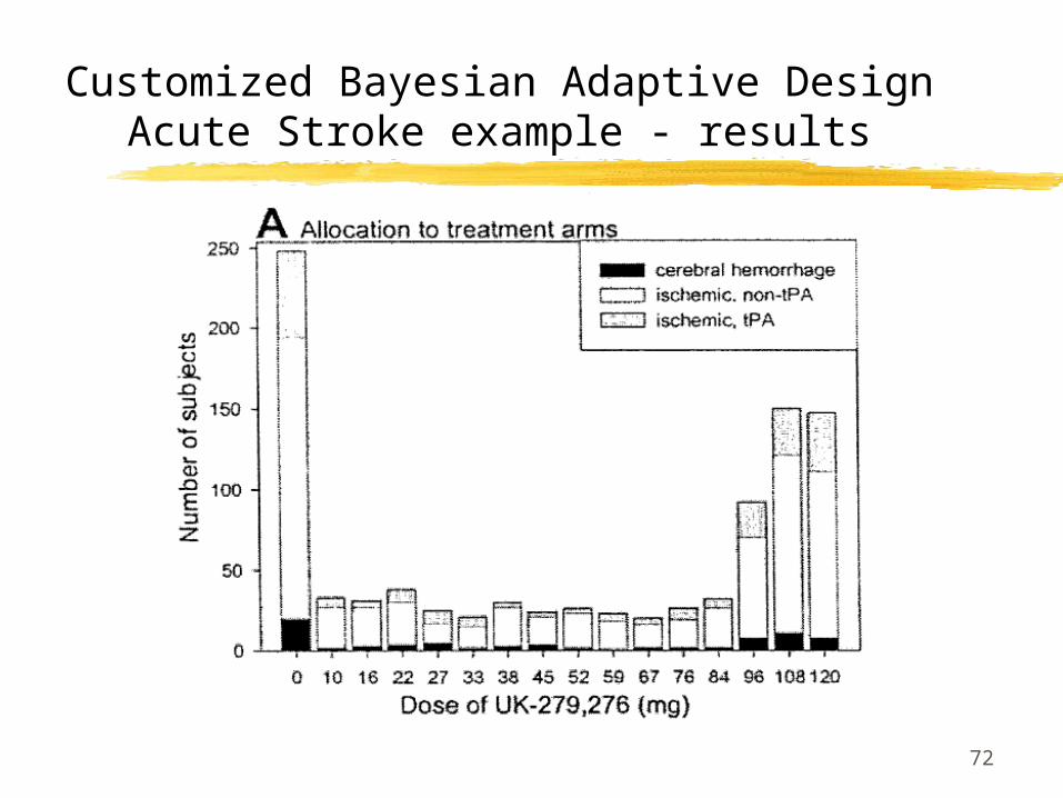
Customized Bayesian Adaptive DesignAcute Stroke example (ASTIN Trial)
Single IV infusion of UK-279,276 (neutrophil inhibitory factor) or placebo within 6 hours of stroke symptom onset
Bayesian sequential design with real-time efficacy data capture Continuous reassessment of dose-response
Patients randomized to Placebo (at least 15%), or The 1 of 15 doses which minimizes expected variance of
ED95 response
Krams, et al. STROKE (2003)
70
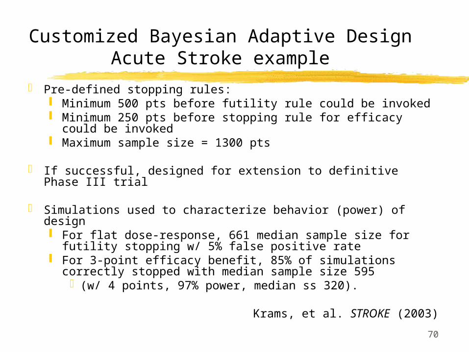
Customized Bayesian Adaptive DesignAcute Stroke example
Pre-defined stopping rules: Minimum 500 pts before futility rule could be invoked Minimum 250 pts before stopping rule for efficacy could
be invoked Maximum sample size = 1300 pts
If successful, designed for extension to definitive Phase III trial
Simulations used to characterize behavior (power) of design For flat dose-response, 661 median sample size for futility
stopping w/ 5% false positive rate For 3-point efficacy benefit, 85% of simulations correctly
stopped with median sample size 595 (w/ 4 points, 97% power, median ss 320).
Krams, et al. STROKE (2003)
71
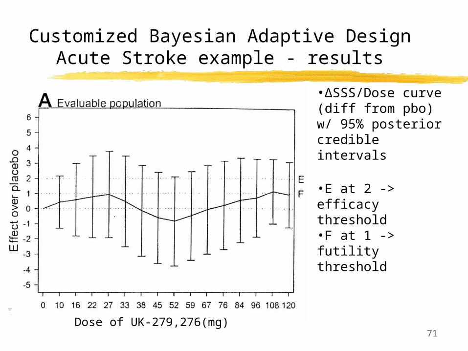
Customized Bayesian Adaptive DesignAcute Stroke example - results
•ΔSSS/Dose curve (diff from pbo) w/ 95% posterior credible intervals
•E at 2 -> efficacy threshold•F at 1 -> futility threshold
Dose of UK-279,276(mg)
72
Customized Bayesian Adaptive DesignAcute Stroke example - results
73
Adaptive crossover additional simulation results
74
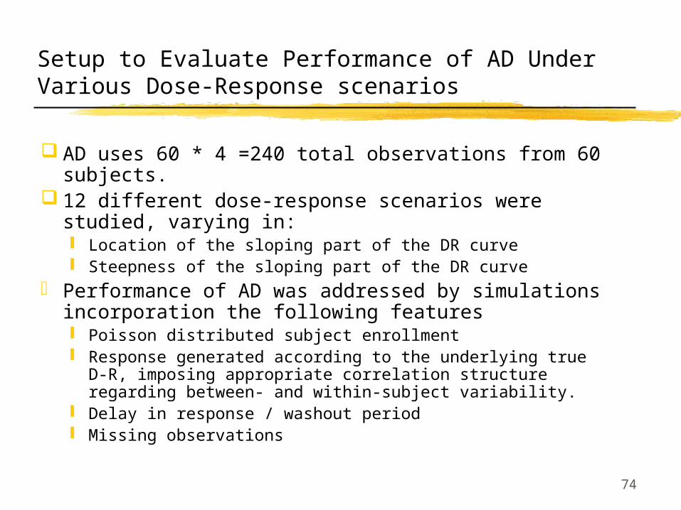
Setup to Evaluate Performance of AD Under Various Dose-Response scenarios
AD uses 60 * 4 =240 total observations from 60 subjects.
12 different dose-response scenarios were studied, varying in: Location of the sloping part of the DR curve Steepness of the sloping part of the DR curve
Performance of AD was addressed by simulations incorporation the following features Poisson distributed subject enrollment Response generated according to the underlying true D-R,
imposing appropriate correlation structure regarding between- and within-subject variability.
Delay in response / washout period Missing observations
75
Performance of Selected AD
Key criteria for evaluation included
Subject allocation pattern Power for testing superiority of a dose level versus
placebo; Type I error Dose selection properties ( right identification of D-
R plateau ) Simultaneous confidence interval methodology for
isotonic regression is developed in the literature and can be used for dose-response curve estimation
76
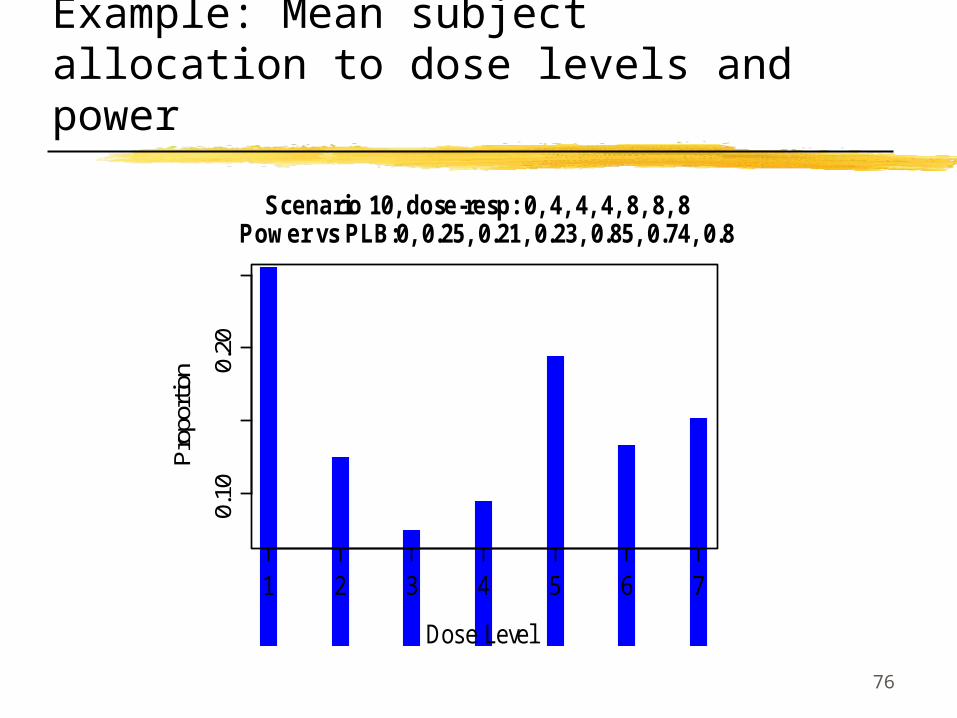
Example: Mean subject allocation to dose levels and power
1 2 3 4 5 6 7
0.10
0.20
Scenario 7, dose-resp: 0, 8, 8, 8, 8, 8, 8 Power vs PLB:0, 0.75, 0.61, 0.56, 0.85, 0.49, 0.79
Dose Level
Pro
porti
on
1 2 3 4 5 6 7
0.10
0.15
0.20
0.25
Scenario 8, dose-resp: 0, 4, 4, 4, 4, 4, 8 Power vs PLB:0, 0.26, 0.21, 0.23, 0.31, 0.27, 0.8
Dose Level
Pro
porti
on
1 2 3 4 5 6 7
0.10
0.15
0.20
0.25
Scenario 9, dose-resp: 0, 4, 4, 4, 4, 8, 8 Power vs PLB:0, 0.26, 0.22, 0.23, 0.31, 0.72, 0.83
Dose Level
Pro
porti
on
1 2 3 4 5 6 7
0.10
0.20
Scenario 10, dose-resp: 0, 4, 4, 4, 8, 8, 8 Power vs PLB:0, 0.25, 0.21, 0.23, 0.85, 0.74, 0.8
Dose Level
Pro
porti
on
1 2 3 4 5 6 7
0.10
0.20
Scenario 11, dose-resp: 0, 4, 4, 8, 8, 8, 8 Power vs PLB:0, 0.23, 0.2, 0.69, 0.85, 0.72, 0.79
Dose Level
Pro
porti
on
1 2 3 4 5 6 7
0.10
0.15
0.20
0.25
Scenario 12, dose-resp: 0, 4, 8, 8, 8, 8, 8 Power vs PLB:0, 0.22, 0.61, 0.7, 0.83, 0.69, 0.75
Dose Level
Pro
porti
on
77
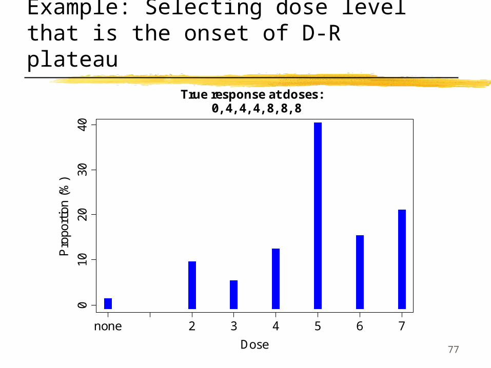
Example: Selecting dose level that is the onset of D-R plateau
010
2030
40True response at doses:
0, 4, 4, 4, 8, 8, 8
Dose
Pro
port
ion
(%)
none 2 3 4 5 6 7
78
Conclusions From Simulations
On average, the algorithm allocates subjects to the neighborhood of the effective and the highest sub-effective dose levels for the studied D-R scenarios. Depending on the underlying dose-response scenario,
the average number of observations on the dose with highest number of subjects ranged from 43 to 60.
Good estimation of the D-R plateau on set High power to declare effective and highest sub-effective
dose levels superior to placebo. Depending on the scenario, the power of the AD to
declare the dose with highest number of subjects significantly different from placebo ranged from 75 to 91% with most scenarios yielding power 80% or greater.