arX

iv:1

206.

3988

v1 [

cs.N

I] 1

8 Ju

n 20

121

Cooperative localization using angle of arrivalmeasurements: sequential algorithms and

non-line-of-sight suppressionBharath Ananthasubramaniam and Upamanyu Madhow

Electrical and Computer Engineering DepartmentUniversity of California, Santa Barbara

Santa Barbara, CA 93106E-mail: bharath@engr.ucsb.edu, madhow@ece.ucsb.edu

Abstract

We investigate localization of a source based on angle of arrival (AoA) measurements made at a geographicallydispersed network of cooperating receivers. The goal is to efficiently compute accurate estimates despiteoutliers inthe AoA measurements due to multipath reflections in non-line-of-sight (NLOS) environments. Maximal likelihood(ML) location estimation in such a setting requires exhaustive testing of estimates from all possible subsets of“good” measurements, which has exponential complexity in the number of measurements. We provide a randomizedalgorithm that approaches ML performance with linear complexity in the number of measurements. The buildingblock for this algorithm is a low-complexity sequential algorithm for updating the source location estimates underline-of-sight (LOS) environments. Our Bayesian frameworkcan exploit the ability to resolve multiple paths inwideband systems to provide significant performance gains over narrowband systems in NLOS environments, andeasily extends to accommodate additional information suchas range measurements and prior information aboutlocation.

Index Terms

Cooperative localization, Non-line-of-sight suppression, Robust estimation, Angle of arrival measurements, Bayesianframework

I. INTRODUCTION

In this paper, we investigate cooperative localization of asource transmitting a known signal using a networkof geographically dispersed receivers (detectors) using angle of arrival (AoA) measurements. We consider AoAmeasurements, since they only require that each receiver has a calibrated antenna array with known orientation andlocation, and that the receivers can coordinate to pool all the AoA estimates corresponding to a given source (e.g.,using coarse timing synchronization between the receiversto associate AoAs for the signal from a given source at agiven point of time). While the geometry of AoA-based sourcelocalization is straightforward for line-of-sight (LOS)environments, our primary goal in this paper is to develop efficient localization algorithms for non-line-of-sight(NLOS) environments.

While the problem considered here is of broad applicability, our primary motivation is localization in sensornetworks, where a network of collector nodes (i.e., data gathering nodes with some advanced capabilities such asAoA estimation) collaboratively decode and localize transmissions from elementary microsensors that have datato send. Since sensors communicate only when they observe an“interesting” event, without prior coordinationwith the collector nodes, thissensor-drivenparadigm (proposed in [1]), allows drastic reduction in themicrosensorfunctionality and communication energy costs. By locatingthe sensors transmitting in response to the event, thelocation of the event can be estimated. Our goal, therefore,is to locate the transmitting sensor in NLOS propagationconditions. Note that the term ‘sensor’ is not a reference toreceivers, as is sometimes the usage in the sourcelocalization and array processing literature. To avoid confusion, we use the term “source” to refer to the source ofthe transmitted signal, and the term “receiver” for a devicethat receives this signal and produces an AoA estimate.

2

This problem is also applicable to asset tracking using active radio frequency identification (RFID) tags, in whichtags periodically or intermittently transmit a signal to beused to localize them [2], [3], [4].

In the preceding scenario, other measurements such as time-difference-of-arrival (TDOA) [2] and received signalstrength (RSS) [5] could also be used for localization. TDOAmeasurements require stringent synchronizationbetween the receivers, while RSS measurements are highly sensitive to the propagation environment, and typicallyrequire extensive calibration. On the contrary, AoA measurements offer the prospect of providing accurate localiza-tion without tight coordination among receivers or extensive calibration, at least in LOS environments. In this paper,we investigate whether this promise can be realized in more realistic NLOS environments, with the understandingthat AoA-based performance can be augmented by incorporating information from TDOA and RSS measurements,if available.

We previously proposed one possible receiver design (including timing acquisition and array processing algo-rithms) to generate these AoA estimates [1]. In this paper, we abstract away such details in order to focus onthe fundamentals of AoA-based localization. To this end, wepropose statistical models for AoA measurementsthat model the performance of a broad class of AoA estimatorsin the literature under a variety of propagationenvironments. These models permit performance comparisons between our proposed algorithms and fundamentallimits such as the Cramer-Rao Lower Bound (CRLB). Our main contributions are as follows:

1) As a building block for localization in NLOS environments, we develop ascalable sequential algorithmfor aggregation of AoA estimates from multiple receivers toestimate the source location in LOS scenarios(minimal multipath scattering). The receivers only need toexchange source location and covariance estimates,where the source location estimate is updated with the localAoA measurement before it is forwarded to thenext receiver. This approximately maximum likelihood (ML)algorithm has linear complexity in the numberof receivers. We use the CRLB to estimate the location uncertainty as a function of the coverage area, thevariance of the AoA measurements, and the number of receivers.

2) We model the AoA estimates due to multipath components with AoA measurements far away from theLOS path asoutliers. Assuming that at least some of the receivers see near-LOS paths, ML localizationrequires brute force elimination of outliers by considering all possible subsets of AoA measurements, which isexcessively complex. We propose a randomized algorithm with O(MN2) complexity foroutlier suppression,which employsM randomly initialized instances of the sequential algorithm. HereM is chosen to achievea given probability of localization failure, and does not grow with N , the number of receivers.

3) The proposed algorithms are numerically shown to achievethe CRLB and the ML performance. We quantifythe performance penalty due to the presence of outliers, andprovide examples that illustrate the performanceadvantage of wideband systems, which can resolve LOS and NLOS paths, relative to narrowband systemswithout the capability for providing such resolution. Also, our Bayesian framework permits integration ofother sensing modalities such as RSS-based range measurements for localization in a NLOS environment.

An outline of these preceding results was presented previously at a workshop [6]. This paper significantly expandsupon that work, including detailed derivations of the algorithms and performance bounds, as well as a morecomprehensive set of simulation results.

Related Work: There is a rich history of literature on source localizationusing a variety of measurements,including TDOA, AoA and RSS that depend on LOS channels between the source and the receivers with nomultipath and consider errors due to measurement noise alone. A detailed discussion of the body of standardlocalization techniques using multiple modalities, theirlimitations and practical considerations are presented in[7],[8].

Our approach to localization in NLOS environments draws upon the significant literature on handling outliers[9]. One approach is to identify and remove outliersbefore location estimation. In [10], a generalized likelihoodratio test is used to identify NLOS estimates; this assumes at least partial statistical knowledge about the NLOScomponents and does not utilize the inherent consistency between measurements corresponding to a single source.Prior knowledge of the NLOS characteristics is used to eliminate outliers in TDOA and AoA measurements in[11], but requires exploring all subsets of measurements, which is not scalable. The skewed distribution of range

3

or time of flight (TOF) estimates due to a positive bias introduced by NLOS propagation is used in [12] to identifyand correct for NLOS errors. Correction of NLOS time of arrival estimates prior to localization is accomplished byKalman filtering in [13] and soft combining of pseudo-range measurements in [14]. The residuals from locating thesource using a least-squares algorithm on a set of AoA measurements are compared against a threshold to identifyand eliminate outliers in [15]. More recently, Yu et al. [16]formulate a Neyman-Pearson test to only identifythe outliers in different combinations of localization measurements such as AoA, ToA and RSS-based rangingand similarly, Guvenc et al. [17] identify NLOS components in multipath ultrawideband (UWB) channel metricsusing joint likelihood ratio tests. Al-Jazzar et al. [18] design a nonlinear optimization algorithm with nonlinearconstraints to compute the locations of the unknown scatterers to identify the NLOS components. Guvenc et al.present a detailed survey of UWB TOA-based NLOS mitigation techniques in [19].

In this paper, we adopt the alternative approach of robust location estimation while simultaneously limiting theeffect of outliers (called NLOS “mitigation”), thus eliminating outliers “on the go.” To the best of our knowledge thisapproach has only once been used with AoA measurements in [20] and similar work for range/TOF measurementsincludes [21], [22], [23]. Tang et al. [20] formulate the localization using AoA and ToA as an optimization with ageometrically-constrained objective function that has a higher computational complexity of at leastO(N3). Moresignificantly, they only consider angular spreads due to a disk of scatterers around the transmitter that results in asimple Gaussian model of AoA spread. Thus, this AoA distribution is equivalent to having Gaussian errors in theLOS estimate and does not account for blockage of LOS. Chen [21] proposes a weighted least-squares localizationusing range/TOF measurements, where the weights are iteratively varied to assign the lowest weights to outliers andhighest to the LOS estimates. The main drawback of this approach is theO(2N ) complexity due to a combinatorialexploration of subsets of “good” measurements, which does not scale. Venkatesh and Buehrer [22] present a linearprogramming approach (of approximatelyO(N3) complexity) to mitigate NLOS using ToA estimates in a UWBsystem that utilizes the positive bias in NLOS range measurements.

Our approach shares many similarities with Casas et al. [23]. Casas et al. perform closed-form trilateration ofrandom triplets of measurements (similar to theM randomizations in our method) followed by a selection ofthe location estimate with the smallest median residual, which has anO(MN) complexity. They propose a slightimprovement by performing a multilateration after identification of the outliers from the previous step, incurring anO(N2) complexity. However, localization even without outliers using AoA measurements does not have a closedform solution in terms of more than two noisy AoA measurements in two-dimensions (and more than three noisyAoA measurements in three-dimensions), i.e., in an over specified system, due to the trigonometric dependenceof AoA on the source location. This nonlinear dependence of AoA on the source location makes the algorithmiccomplexity inherently larger than for the time of flight measurements considered in [23]. Our sequential algorithmoffers a low-complexity approach to localization, which can be viewed as a generalization of [23]: we naturallygrow “good” subsets of measurements to include many LOS measurements, without needing a separate phasefor localization using inliers. Furthermore, our Bayesianframework permits incorporation of other localizationmodalities, such as RSS-based range measurements, with little change to the algorithm (see Figure 4).

The rest of the paper is organized as follows. AoA measurement models under different propagation environmentsare described in Section II. The sequential algorithm for localization in LOS scenarios, along with performancebenchmarks, are presented in Section III. We derive an extension to the sequential localization to suppress NLOSAoA estimates in Section IV, which is motivated by the structure of the ML estimate. The proposed algorithmsare numerically investigated in Section V. Section VI contains concluding remarks.

II. M ODELS OFAOA ESTIMATES

Each receiver estimates the direction of arrival of the source transmission using an antenna array. In this section,we discuss models for the estimated AoA that capture the effects of LOS and NLOS propagation environments.These models are then used to design source localization algorithms in Sections III and IV. For simplicity, weassume a linear array, although our framework generalizes to arbitrary antenna arrays, as long as the array manifoldis known.

4

Classical AoA estimation techniques such as MUSIC and ESPRIT [24] are designed to separate uncorrelated pointsources assuming LOS propagation from the source to the receivers. This point-source propagation model does notaccount for multipath scattering encountered in many deployment environments. Multipath adds highly correlatedAoA components to the received signal, and extensions to deal with such effects using techniques such as spatialsmoothing have been proposed at the cost of lower AoA resolutions and poorer source separation capabilities.

Here, we adopt the approach taken in [25], [26], [27], [28], [29], where a series of models for AoA estimationin the presence of scattering have been proposed. The propagation is characterized by a mean arrival angle(corresponding to the true bearing) and a spatial spreadingparameter (quantifying the spatial uncertainty causedby multipath). The resulting AoA at the antenna array is a random variable, typically modeled as Gaussian [28] orLaplacian [30]. Drawing on these ideas, we propose the following models:

LOS model: We characterize the spatial spreading in LOS propagation scenarios by zero-mean symmetric finitevariance “noise” models, such as the Gaussian and Laplacian. AoA estimation under LOS in the presence of additivewhite Gaussian noise results in zero-mean Gaussian errors,whose variance depends on the signal-to-noise ratio [31].Additional errors in the AoA measurements due to local scattering in the vicinity of the source are also modeledusing zero-mean symmetric distributions. Therefore, Gaussian and Laplacian error models seamlessly transitionbetween scenarios with and without local scattering for different values of the spatial spreading parameter. Thesemodels represent situations where the received signal has astrong LOS component, together with a limited amountof scattering. For a source at locationX along a true bearingθ(X), the Gaussian LOS model with local scatteringis

pGaus(θ/X) =1√

2πσ(1− 2Q( π2σ ))

exp

(

−(θ − θ(X))2

2σ2

)

, θ ∈[

−π

2,π

2

]

, (1)

whereσ2 represents the spatial extent of scattering,Q(t) =∫∞t

exp(−t2/2)dt/√2π is the normal tail distribution

and all angles are measured with respect to the antenna broadside. The permissible angles are within±π/2 ofthe antenna broadside and the Gaussian density is truncatedto reflect this. As the spatial spreadσ2 increases,the density become progressively long tailed and tends toward a uniform density. The Laplacian LOS model withspatial spreading factorσ has heavier tails than the Gaussian model:

pLap(θ/X) =1

2√2σ exp(−|π/(

√2σ)|)

exp

(

−√2|θ − θ(X)|

σ

)

, θ ∈[

−π

2,π

2

]

. (2)

LOS blockage model: Environments where the LOS path to a receiver is blocked by structures, such as building,hills or trees, are also relevant. As a result, the received signal is composed exclusively of multipath componentsthat deviate “far” from the LOS path. Therefore, AoA measurements made from these scattered and reflected pathsalone are fairly uncorrelated with the true bearing of the source. An AoA estimate drawn uniformly from thefeasible set aptly models such a scenario:

pNLOS(θ/X) =1

π, θ ∈

[

−π

2,π

2

]

. (3)

When there are significant contributions from both the LOS path and the multipath components from otherdirections, the model for the AoA estimates depends on the capability of the receiver to resolve these contributionsspatially. If the source signal has a large enough bandwidth, the multipath components can be resolved in time, andseparate AoA estimates can be obtained for each path. If the bandwidth is insufficient to resolve the paths, thenthe receiver may only be able to obtain a single AoA estimate.We model these two scenarios separately.

Narrowband multipath model: With narrowband source transmissions, the receiver is capable of resolving thearriving combination of LOS path and NLOS multipath in the spatial domain only. For receivers with relativelysmall number of antenna elements, the receiver can only measure the AoA of the strongest arriving path (orstrongest superposition of paths). Hence, each receiver produces a single AoA estimate that, depending on therelative strengths of the LOS and NLOS components, will provide an estimate close to or very “far” from the truebearing of the source (outliers). Accordingly, we model a typical narrowband scenario as follows: Letα be the

5

fraction of receivers that experience reflected and scattered multipath significantly stronger than the LOS path. Inthis event, the AoA appears to correspond to the LOS path being blocked and hence, is drawn from the worst-caseNLOS model in (3). In the remaining instances, when the LOS path is strong, the AoA is drawn from one of theLOS models, for instance (1). Thus, we arrive at the following narrowband model:

pnarrowband(θ/X) = α pNLOS(θ/X) + (1− α) pGaus(θ/X). (4)

This model also represents the least favorable multipath environment, where the LOS component is either presentand significant, or is blocked (completely absent), and serves as our candidate model for developing the NLOSsuppression algorithm. Note that distributions with heavy-tails, such as the Laplacian (in (2)) or a Cauchy model,can also be used to represent the narrowband setting with outliers. We investigate these alternate models in SectionV-B.

Wideband multipath model: With wideband source transmissions, the receiver has an additionally resolve pathsin time as well. When the scattered or reflected paths are sufficiently temporally or spatially separated from theLOS path, the receiver is capable of resolving the LOS path, and possibly multiple NLOS paths. We model themultiple AoA estimates produced by the receiver as follows:the AoA estimate corresponding to the LOS pathis represented by an LOS model such as (1) or (2), while the remaining estimates are drawn uniformly from thefeasible set, as in the worst-case model with LOS blockage. Thus, if a receiver resolvesL paths, the resulting AoAestimates are generated according to the following distribution:

pwideband(ˆθ(1), ˆθ(2) . . . ˆθ(L)/X) = pGaus(

ˆθ(1)/X) pNLOS(ˆθ(2)/X) . . . pNLOS(

ˆθ(L)/X). (5)

Assuming that the LOS path is not blocked, it is resolved by a receiver in the wideband scenario. However, it isnot knowna priori which of theL AoA estimates corresponds to the LOS path. If the LOS path is blocked, thennone of theL resolved AoA estimates might be close to the true source bearing.

Estimate SLE and ECM using

AoA at 2 random receivers in

polar coordinates (see left)

Transform to global

cartesian coordinates

Update SLE and ECM using

local AoA measurements and

LMMSE updates

Transform to local

polar coordinates

Pas

s pri

ors

to n

ext

rece

iver

unti

l al

l A

oA

are

use

d

At each receiver

For M random receiver pairs, estimate

initial SLE and ECM, update lists of

aggregated and remaining receivers

Compute angular errors for

remaining receivers and find

one with smallest angular error

Obtain new candidate SLE and ECM

using AoA from that receiver and check

if all angular errors are below threshold

If yes, make candidate the new SLE

and ECM, and update the two lists

else, do not consider this receiver again

Conti

nue

unti

l no A

oA

pro

duci

ng a

ngula

r

erro

r bel

ow

thre

shold

are

lef

t

R1R8

R7

R6

R5

R3

R2

R4

+source

location

estimated

location +

X

Y

polar coordinates of receiver 1

polar coordinates of receiver 2

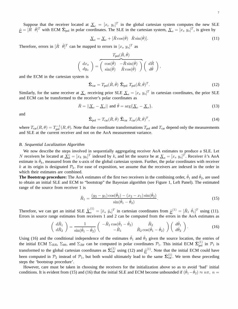
Fig. 1. (Left panel) One possible sensor network layout with a circular field and8 receivers on its perimeter: The geometry used to computethe “bootstrap” source estimate from AoA estimates of receivers R1 and R2 is shown. (Center Panel) The flowchart of the sequentiallocalization algorithm using AoA measurements (with no outliers) presented in Section III-B. (Right Panel) The flowchart of the outliersuppresion algorithm in Section IV-B that uses the sequential algorithm in theCenter Panel.

III. L OCALIZATION IN LOS SCENARIOS

In this section, we consider scenarios with only LOS propagation, i.e., no LOS blockage, where the spread inthe AoA estimates is caused only by local scattering. We present an algorithm for sequential aggregation of theavailable AoA estimates (generated according to the LOS model in Section II) to produce the estimate of thesource location. Each receiver performs linear minimum mean squared error (LMMSE) updates on theprior sourcelocation estimate (SLE) (received from a previous receiver) using its own AoA estimate, before passing the updated

6

estimate to the next receiver. This process is continued until all the available AoA estimates is aggregated into theSLE.

A. LMMSE Updates and Coordinate Transformations

At each receiver, we desire linear updates (to keep the computational burden to a minimum) for arbitrarymeasurement models, while also propagating only the first- and second-order statistics of the sensor location.Both these requirements are satisfied by an LMMSE estimator.Working with AoA measurements at each receiver,the SLE updates are conveniently formulated in the polar coordinates[R θ] centered at that receiver, whereR is thedistance between the source and receiver, andθ is measured from the x-axis (see Figure 1, Left Panel). Additionally,this choice of polar coordinates makes the LMMSE update optimal under Gaussian measurement models such asthe LOS model in Section II.

Each receiver receives the following prior information: SLE µ = [R θ]T and ECMΣ, where

Σ =

(ΣRR ΣRθ

ΣRθ Σθθ

)

.

The AoA estimate at the receiver isθ with spatial spreadσθ. Note, henceforth, we use the convention that newmeasurements are represented by., prior information by., update variables by., vectors by. and matrices by boldtypeface. We desire a linear SLE update,

µ = µ+K(θ −Aµ), (6)

whereK is the Kalman gain andA = [0 1] (only new AoA estimates are available at the receiver). For theinnovation(θ −Aµ) to be orthogonal to the estimateµ, the Kalman gain must be:

K = AΣ (σθ +AΣAT )−1. (7)

Therefore, inserting (7) into (6), the updated SLE,µ, is obtained as

R = R+ΣRθ(θ − θ)

Σθθ + σθ,

θ =Σθθ θ + σθ θ

Σθθ + σθ. (8)

The ECM update can be obtained using (6) as

Σ−1 = Σ

−1 +

(0 00 (σθ)

−1

)

. (9)

The entries of the updated ECM are given by

ΣRR = ΣRR − (ΣRθ)2

Σθθ + σθ,

1

Σθθ

=1

Σθθ

+1

σθand ΣRθ =

σθ ΣRθ

Σθθ + σθ. (10)

When the observationsθ have Gaussian errors as in the LOS model (1), the LMMSE updates in (8) are also theoptimal minimum mean squared error updates. Under non-Gaussian error models, the LMMSE updates are theoptimal linear updates from the perspective of mean squarederror.

The updated SLEµ and ECMΣ are thus produced in a polar coordinate system centered at the receiver with thenew measurement. This SLE and ECM must then be transformed tothe global cartesian system (a common frameof reference) to provide the information in a form accessible to the next receiver. The next receiver then transformsthese estimates into its own polar coordinate system. We nowdescribe transformations between the local polarcoordinate and global cartesian coordinate systems.

7

Suppose that the receiver located atXc = [xc yc]T in the global cartesian system computes the new SLE

µ = [R θ]T with ECM Σpol in polar coordinates. The SLE in the cartesian system,Xs = [xs ys]T , is given by

Xs = Xc + [R cos(θ) R sin(θ)]. (11)

Therefore, errors in[R θ]T can be mapped to errors in[xs ys]T as

(dxsdys

)

=

Tpol(R, θ)︷ ︸︸ ︷(

cos(θ) −R sin(θ)

sin(θ) R cos(θ)

)(dR

dθ

)

,

and the ECM in the cartesian system is

Σcar = Tpol(R, θ) Σpol Tpol(R, θ)T . (12)

Similarly, for the same receiver atXc receiving prior SLEXs = [xs ys]T in cartesian coordinates, the prior SLE

and ECM can be transformed to the receiver’s polar coordinates as

R = ||Xc −Xs|| and θ = arg{Xc −Xs}, (13)

andΣpol = Tcar(R, θ) Σcar Tcar(R, θ)T , (14)

whereTcar(R, θ) = T−1pol (R, θ). Note that the coordinate transformationsTpol andTcar depend only the measurements

and SLE at the current receiver and not on the AoA measurementvariance.

B. Sequential Localization Algorithm

We now describe the steps involved in sequentially aggregating receiver AoA estimates to produce a SLE. LetN receivers be located atXc

k = [xk yk]T indexed byk, and let the source be atXs = [xs ys]

T . Receiverk’s AoAestimate isθk, measured from the x-axis of the global cartesian system. Further, the polar coordinates with receiverk at its origin is designatedPk. For ease of exposition, we assume that the receivers are indexed in the order inwhich their estimates are combined.The Bootstrap procedure: The AoA estimates of the first two receivers in the combining order, θ1 andθ2, are usedto obtain an initial SLE and ECM to “bootstrap” the Bayesian algorithm (see Figure 1, Left Panel). The estimatedrange of the source from receiver 1 is

R1 =(y2 − y1) cos(θ2)− (x2 − x1) sin(θ2)

sin(θ1 − θ2). (15)

Therefore, we can get an initial SLEX(1)s = [xs ys]

T in cartesian coordinates fromµ(1) = [R1 θ1]T using (11).

Errors in source range estimates from receivers 1 and 2 can becomputed from the errors in the AoA estimates as(

dR1

dR2

)

=1

sin(θ1 − θ2)

(−R1 cos(θ1 − θ2) R2

−R1 R2 cos(θ1 − θ2)

)(dθ1dθ2

)

. (16)

Using (16) and the conditional independence of the estimates θ1 and θ2 given the source location, the entries ofthe initial ECM ΣRR, Σθθ, andΣRθ can be computed in polar coordinatesP1. This initial ECM Σ

(1)pol in P1 is

transformed to the global cartesian coordinates asΣ(1)car using (12) andµ(1). Note that the initial ECM could have

been computed inP2 instead ofP1, but both would ultimately lead to the sameΣ(1)car. We term these preceding

steps the ‘bootstrap procedure’.However, care must be taken in choosing the receivers for theinitialization above so as to avoid ‘bad’ initial

conditions. It is evident from (15) and (16) that the initialSLE and ECM become unbounded if(θ1− θ2) ≈ nπ, n =

8

0, 1, . . ., due to thesin(θ1 − θ2) term in the denominator of both equations. Thus, the error islargest when thesource is roughly collinear with the two receivers (on the line joining the two receivers), when the nominal AoAmeasurements are close to being parallel or antiparallel. Therefore, the algorithm is always initialized with a pair ofreceivers withθ1 − θ2 significantly different from0 or π, which also ensures that the initial SLE is mostly withinthe ring of receivers. This idea is similar to the concept of dilution of precision in the global positioning system[32] that describes the effect of the satellite configuration on the location accuracy. Thereafter, the receivers can becombined in any random order and effect of this order on performance is simulated in Section V-A.

The sequential algorithm for source localization has the following steps:Step 1 (Bootstrap):Estimate initial SLEµ(1) and ECMΣ

(1)pol in P1, using (15) and (16). Transform the SLE and

ECM into the global cartesian coordinates asX(1)s andΣ(1)

car, respectively, using (11) and (12). Pass[X(1)s , Σ

(1)car] as

a prior to the next receiver.Step 2 (Transformation):Let the index of the current receiver bek. Transform the prior[X

(k−1)s , Σ

(k−1)car ] to

[µ(k−1), Σ(k−1)pol ] in the local polar coordinate system,Pk, using (13) and (14).

Step 3 (Aggregation):Update the prior estimates[µ(k−1), Σ(k−1)pol ] with the AoA estimate of thekth receiver,θk,

using the LMMSE procedure in (8) and (10). Transform updatedestimates[µ(k), Σ(k)pol ] into the global cartesian

coordinates as[X(k)s , Σ

(k)car ].

Step 4 (Termination):If there are unprocessed AoA measurements, pass priors on tothe next unaggregatedreceiver and go toStep 2. Otherwise output the SLE and stop.

Since only the current SLE and ECM need to be passed on from onereceiver to the next, this algorithm canbe implemented in a distributed manner, with each receiver needing to know only its own location and orientation.While we consider AoA estimates here, this sequential algorithm is quite general, and can, for example, incorporateprobabilistic information on the source range obtained from signal strength measurements. Further, the algorithmis scalable, in that its complexity grows only linearly in the number of receivers. This scalability is required torealize the improvement in localization performance with the number of receivers, details of which are given inSection III-C.

C. ML Estimator and Cramer-Rao Bound

The CRLB is a lower bound on the localization performance of the best minimum variance unbiased estimator.For analytical simplicity, we work with the Gaussian AoA model in (1), although corresponding bounds for othermodels such as the Laplacian in (2) can be easily derived. Forthe Gaussian AoA error model, the log-likelihoodfunction (within scale factors and constants) for the observed AoA estimates{θi}Ni=1 given the source locationX = (x, y) is

L(θ1, θ2, . . . , θN/X) = −N∑

k=1

(θk − θk(X))2

σ2k

, (17)

whereθk(X) is the true bearing of the source from receiverk andσ2 is the AoA spread (estimation error variance)at receiverk. The ML estimator searches for the locationX that maximizes the log-likelihood function in (17),which is a nonlinear least squares problem. For smallσ2

k, the cost function in (17) can be shown to be approximatelyconcave. We have observed numerically that the cost function has an unique global maxima for the parameter valuesof interest and a standard nonlinear least squares solver (such as the “lsqnonlin” function in MatlabR© with defaultparameters that is based on [33]) produces the ML estimate. The ML estimate is shown to achieve the CRLB inSection V-A.

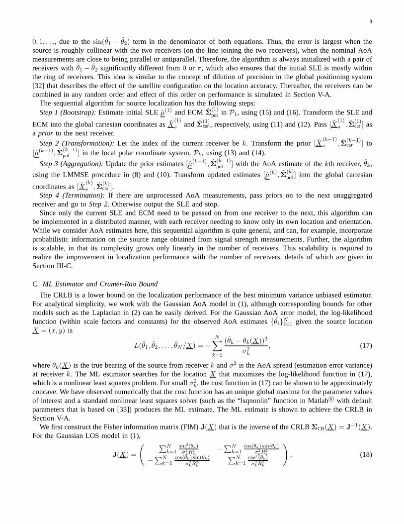
We first construct the Fisher information matrix (FIM)J(X) that is the inverse of the CRLBΣCR(X) = J−1(X).

For the Gaussian LOS model in (1),

J(X) =

( ∑Nk=1

sin2(θk)σ2

kR2

k

−∑Nk=1

cos(θk) sin(θk)σ2

kR2

k

−∑Nk=1

cos(θk) sin(θk)σ2

kR2

k

∑Nk=1

cos2(θk)σ2

kR2

k

)

, (18)

9

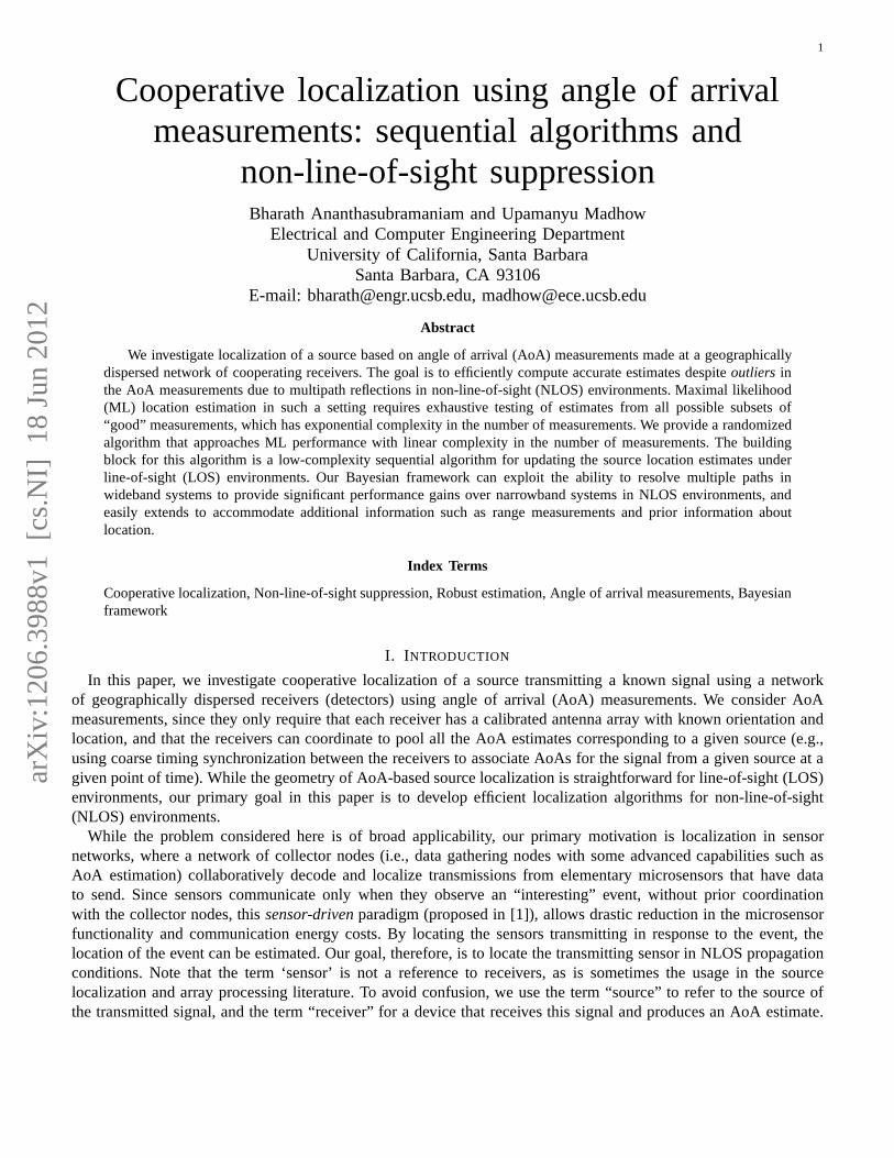
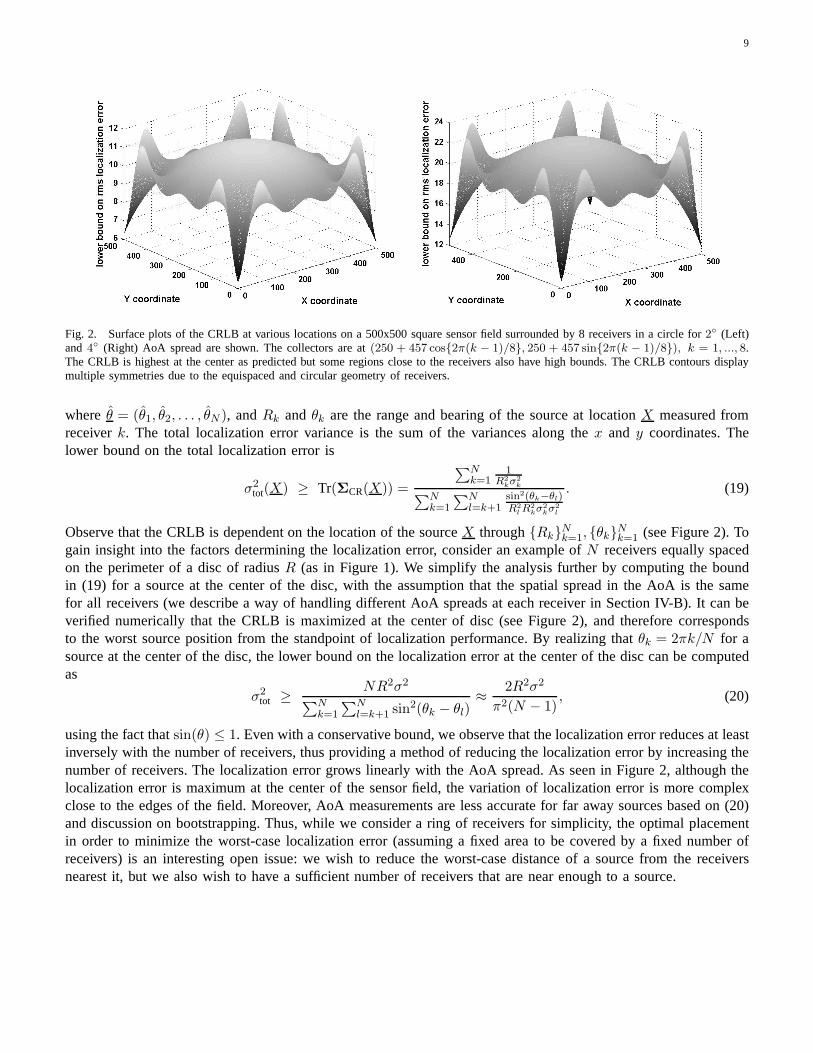
Fig. 2. Surface plots of the CRLB at various locations on a 500x500 square sensor field surrounded by 8 receivers in a circlefor 2◦ (Left)and 4◦ (Right) AoA spread are shown. The collectors are at(250 + 457 cos{2π(k − 1)/8}, 250 + 457 sin{2π(k − 1)/8}), k = 1, ..., 8.The CRLB is highest at the center as predicted but some regions close to the receivers also have high bounds. The CRLB contours displaymultiple symmetries due to the equispaced and circular geometry of receivers.

where θ = (θ1, θ2, . . . , θN ), andRk andθk are the range and bearing of the source at locationX measured fromreceiverk. The total localization error variance is the sum of the variances along thex and y coordinates. Thelower bound on the total localization error is

σ2tot(X) ≥ Tr(ΣCR(X)) =

∑Nk=1

1R2

kσ2

k

∑Nk=1

∑Nl=k+1

sin2(θk−θl)R2

lR2

kσ2

kσ2

l

. (19)

Observe that the CRLB is dependent on the location of the sourceX through{Rk}Nk=1, {θk}Nk=1 (see Figure 2). Togain insight into the factors determining the localizationerror, consider an example ofN receivers equally spacedon the perimeter of a disc of radiusR (as in Figure 1). We simplify the analysis further by computing the boundin (19) for a source at the center of the disc, with the assumption that the spatial spread in the AoA is the samefor all receivers (we describe a way of handling different AoA spreads at each receiver in Section IV-B). It can beverified numerically that the CRLB is maximized at the centerof disc (see Figure 2), and therefore correspondsto the worst source position from the standpoint of localization performance. By realizing thatθk = 2πk/N for asource at the center of the disc, the lower bound on the localization error at the center of the disc can be computedas

σ2tot ≥ NR2σ2

∑Nk=1

∑Nl=k+1 sin

2(θk − θl)≈ 2R2σ2

π2(N − 1), (20)

using the fact thatsin(θ) ≤ 1. Even with a conservative bound, we observe that the localization error reduces at leastinversely with the number of receivers, thus providing a method of reducing the localization error by increasing thenumber of receivers. The localization error grows linearlywith the AoA spread. As seen in Figure 2, although thelocalization error is maximum at the center of the sensor field, the variation of localization error is more complexclose to the edges of the field. Moreover, AoA measurements are less accurate for far away sources based on (20)and discussion on bootstrapping. Thus, while we consider a ring of receivers for simplicity, the optimal placementin order to minimize the worst-case localization error (assuming a fixed area to be covered by a fixed number ofreceivers) is an interesting open issue: we wish to reduce the worst-case distance of a source from the receiversnearest it, but we also wish to have a sufficient number of receivers that are near enough to a source.

10

D. Properties of the Sequential Algorithm

The ML source location is the solution to the non-linear least squares (LS) problem in (17). The solution to thisLS problem is asymptotically (in the number of receiversN ) consistent and efficient, when the observation noiseis Gaussian (e.g., LOS AoA error model in (1)), and the LS solution is asymptotically consistent even when thenoise is non-Gaussian, but with no guarantees on efficiency [34]. The ML estimate can be computed maintainingthe asymptotic consistency and efficiency with the following recursive algorithm [34]:

Xn = Xn−1 + J−1(Xn−1)

∂L(θn/Xn−1)

∂X, n = 2, ..., N, (21)

where Xn is the source location after combining the firstn receiver AoA estimates,J(Xn−1) is the FIM forlocalization with only the firstn− 1 receivers, andL(θn/Xn−1) is the contribution of thenth observation to thelog-likelihood function in (17). As in Section III-C, let[Rn θn]

T represent the current SLEXn−1 in the polarcoordinates centered at receivern. We can now rewrite the recursion for this localization problem as

Xn = Xn−1 + J−1(Xn−1)

(Rn sin(θn)−Rn cos(θn)

)

(θn − θn(Xn−1)), n = 2, ..., N.

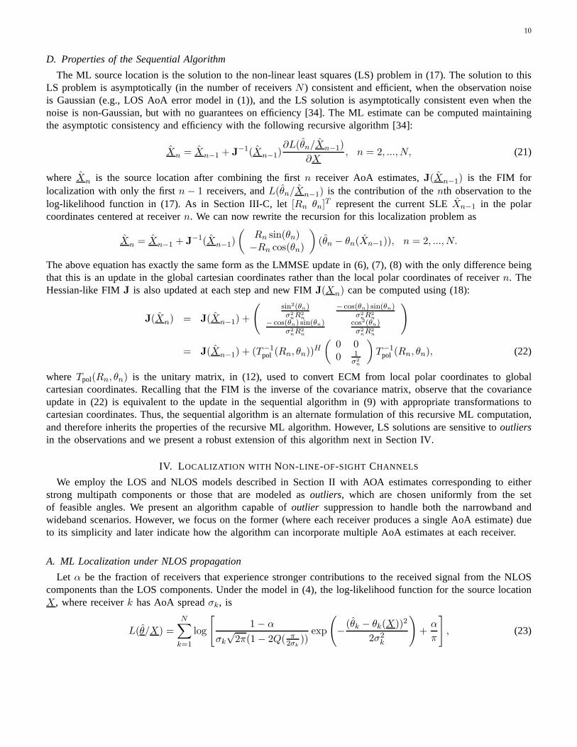
The above equation has exactly the same form as the LMMSE update in (6), (7), (8) with the only difference beingthat this is an update in the global cartesian coordinates rather than the local polar coordinates of receivern. TheHessian-like FIMJ is also updated at each step and new FIMJ(Xn) can be computed using (18):

J(Xn) = J(Xn−1) +

(sin2(θn)σ2

nR2

n

− cos(θn) sin(θn)σ2

nR2

n

− cos(θn) sin(θn)σ2

nR2

n

cos2(θn)σ2

nR2

n

)

= J(Xn−1) + (T−1pol (Rn, θn))

H

(0 00 1

σ2

n

)

T−1pol (Rn, θn), (22)

whereTpol(Rn, θn) is the unitary matrix, in (12), used to convert ECM from localpolar coordinates to globalcartesian coordinates. Recalling that the FIM is the inverse of the covariance matrix, observe that the covarianceupdate in (22) is equivalent to the update in the sequential algorithm in (9) with appropriate transformations tocartesian coordinates. Thus, the sequential algorithm is an alternate formulation of this recursive ML computation,and therefore inherits the properties of the recursive ML algorithm. However, LS solutions are sensitive tooutliersin the observations and we present a robust extension of thisalgorithm next in Section IV.

IV. L OCALIZATION WITH NON-LINE-OF-SIGHT CHANNELS

We employ the LOS and NLOS models described in Section II withAOA estimates corresponding to eitherstrong multipath components or those that are modeled asoutliers, which are chosen uniformly from the setof feasible angles. We present an algorithm capable ofoutlier suppression to handle both the narrowband andwideband scenarios. However, we focus on the former (where each receiver produces a single AoA estimate) dueto its simplicity and later indicate how the algorithm can incorporate multiple AoA estimates at each receiver.

A. ML Localization under NLOS propagation

Let α be the fraction of receivers that experience stronger contributions to the received signal from the NLOScomponents than the LOS components. Under the model in (4), the log-likelihood function for the source locationX, where receiverk has AoA spreadσk, is

L(θ/X) =

N∑

k=1

log

[

1− α

σk√2π(1− 2Q( π

2σk

))exp

(

−(θk − θk(X))2

2σ2k

)

+α

π

]

, (23)

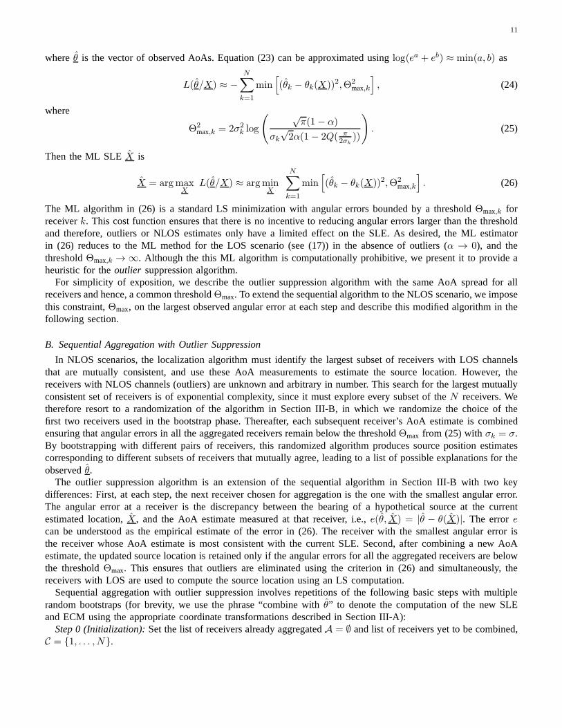
11

whereθ is the vector of observed AoAs. Equation (23) can be approximated usinglog(ea + eb) ≈ min(a, b) as

L(θ/X) ≈ −N∑

k=1

min[

(θk − θk(X))2,Θ2max,k

]

, (24)

where

Θ2max,k = 2σ2

k log

( √π(1− α)

σk√2α(1− 2Q( π

2σk

))

)

. (25)

Then the ML SLEX is

X = argmaxX

L(θ/X) ≈ argminX

N∑

k=1

min[

(θk − θk(X))2,Θ2max,k

]

. (26)

The ML algorithm in (26) is a standard LS minimization with angular errors bounded by a thresholdΘmax,k forreceiverk. This cost function ensures that there is no incentive to reducing angular errors larger than the thresholdand therefore, outliers or NLOS estimates only have a limited effect on the SLE. As desired, the ML estimatorin (26) reduces to the ML method for the LOS scenario (see (17)) in the absence of outliers (α → 0), and thethresholdΘmax,k → ∞. Although the this ML algorithm is computationally prohibitive, we present it to provide aheuristic for theoutlier suppression algorithm.

For simplicity of exposition, we describe the outlier suppression algorithm with the same AoA spread for allreceivers and hence, a common thresholdΘmax. To extend the sequential algorithm to the NLOS scenario, weimposethis constraint,Θmax, on the largest observed angular error at each step and describe this modified algorithm in thefollowing section.

B. Sequential Aggregation with Outlier Suppression

In NLOS scenarios, the localization algorithm must identify the largest subset of receivers with LOS channelsthat are mutually consistent, and use these AoA measurements to estimate the source location. However, thereceivers with NLOS channels (outliers) are unknown and arbitrary in number. This search for the largest mutuallyconsistent set of receivers is of exponential complexity, since it must explore every subset of theN receivers. Wetherefore resort to a randomization of the algorithm in Section III-B, in which we randomize the choice of thefirst two receivers used in the bootstrap phase. Thereafter,each subsequent receiver’s AoA estimate is combinedensuring that angular errors in all the aggregated receivers remain below the thresholdΘmax from (25) withσk = σ.By bootstrapping with different pairs of receivers, this randomized algorithm produces source position estimatescorresponding to different subsets of receivers that mutually agree, leading to a list of possible explanations for theobservedθ.

The outlier suppression algorithm is an extension of the sequential algorithm in Section III-B with two keydifferences: First, at each step, the next receiver chosen for aggregation is the one with the smallest angular error.The angular error at a receiver is the discrepancy between the bearing of a hypothetical source at the currentestimated location,X, and the AoA estimate measured at that receiver, i.e.,e(θ, X) = |θ − θ(X)|. The errorecan be understood as the empirical estimate of the error in (26). The receiver with the smallest angular error isthe receiver whose AoA estimate is most consistent with the current SLE. Second, after combining a new AoAestimate, the updated source location is retained only if the angular errors for all the aggregated receivers are belowthe thresholdΘmax. This ensures that outliers are eliminated using the criterion in (26) and simultaneously, thereceivers with LOS are used to compute the source location using an LS computation.

Sequential aggregation with outlier suppression involvesrepetitions of the following basic steps with multiplerandom bootstraps (for brevity, we use the phrase “combine with θ” to denote the computation of the new SLEand ECM using the appropriate coordinate transformations described in Section III-A):

Step 0 (Initialization):Set the list of receivers already aggregatedA = ∅ and list of receivers yet to be combined,C = {1, . . . , N}.

12

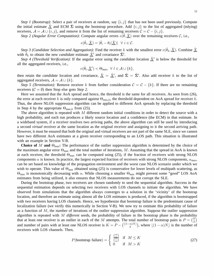
Step 1 (Bootstrap):Select a pair of receivers at random, say{i, j} that has not been used previously. Computethe initial estimateX and ECMΣ using the bootstrap procedure. Add{i, j} to the list of aggregated (inlying)receivers,A = A∪ {i, j}, and remove it from the list of remaining receiversC = C − {i, j}.

Step 2 (Angular Error Computation):Compute angular errorse(θ, X) over the remaining receiversC, i.e.,

e(θi, X) = |θi − θi(X)| ∀ i ∈ C.Step 3 (Candidate Selection and Aggregation):Find the receiverk with the smallest errore(θk, X). CombineX

with θk to obtain the newcandidateestimateX ′ and covarianceΣ′.Step 4 (Threshold Verification):If the angular error using thecandidatelocation X ′ is below the threshold for

all the aggregated receivers, i.e.,e(θl, X

′) < Θmax, ∀ l ∈ A ∪ {k},then retain thecandidatelocation and covariance,X = X ′, and Σ = Σ

′. Also add receiverk to the list ofaggregated receivers,A = A ∪ {k}.

Step 5 (Termination):Remove receiverk from further considerationC = C − {k}. If there are no remainingreceivers (C = ∅) then Stop else gotoStep 2.

Here we assumed that the AoA spread and hence, the threshold is the same for all receivers. As seen from (26),the error at each receiverk is only compared againstΘmax,k, the threshold dependent on AoA spread for receiverk.Thus, the above NLOS suppression algorithm can be applied todifferent AoA spreads by replacing the thresholdin Step 4 by the appropriateΘmax,k from (25).

The above algorithm is repeated withM different random initial conditions in order to detect the source with ahigh probability, and each run produces a likely source location and a confidence (the ECM) in that estimate. Ina wideband system, if a receiver resolves two arriving paths, the above algorithm can still be used by introducinga secondvirtual receiver at the same location as the original receiver and assigning to it the second arriving path.However, it must be ensured that both the original and virtual receivers are not part of the same SLE, since we cannothave two different AoA estimates at a given receiver corresponding to an LOS path. This situation is illustratedwith an example in Section V-B.

Choice of M and Θmax: The performance of the outlier suppression algorithm is determined by the choice ofthe maximum angular errorΘmax and the total number of iterations,M . Assuming that the spread in AoA is knownat each receiver, the thresholdΘmax can be computed using (25), if the fraction of receivers withstrong NLOScomponentsα is known. In practice, the largest expected fraction of receivers with strong NLOS components,αmax,can be set based on knowledge of the propagation environmentand the worst case NLOS scenario under which wewish to operate. This value ofΘmax obtained using (25) is conservative for lower levels of multipath scattering, asΘmax is monotonically decreasing withα. While choosing a smallerΘmax might prevent some “good” LOS AoAestimates from being utilized, it also ensures that NLOS measurements do not corrupt the SLE.

During the bootstrap phase, two receivers are chosen randomly to seed the sequential algorithm. Success in thesequential estimation depends on selecting two receivers with LOS channels to initiate the algorithm. We haveobserved from simulations that the algorithm always converges to a solution in the ‘vicinity’ of the bootstraplocation, and therefore an estimate using almost all the LOSestimates is produced, if the algorithm is bootstrappedwith two receivers having LOS channels. Hence, we hypothesize that bootstrap failure is the predominant cause oflocalization failure (we verify this numerically in Section V-B). We now try to estimate this probability of failureas a function ofM , the number of iterations of the outlier suppression algorithm. Suppose the outlier suppressionalgorithm is repeated withM different seeds, the probability of failure in the bootstrap phase is the probabilitythat at least one receiver is an outlier in each of theM attempts. The total number of bootstrap pairs isP =

(N2

)

and number of pairs with at least one NLOS receiver isK = P −(⌊(1−α)N⌋

2

), where⌊(1−α)N⌋ is the number of

receivers with LOS channels. Then,

P (bootstrap failure) =

{(MK)

(P

M)

if M ≤ K

0 if M > K(27)

13

When the receivers resolve multiple arriving paths, the above probability of failure computation is modified byreplacing the number of receivers by the total number of resolved paths. Depending on the probability of failureacceptable in the system, (27) is used to choose the number ofrandomizations of the algorithm that are necessary.

A practical issue of interest is the choice of the number of randomizationsM for different total number ofreceiversN to achieve a fixed probability of bootstrap failure under similar NLOS propagation environments (fixedα). Rearranging the tight upper bound on the probability of bootstrap failure, presented in the Appendix as (30),we get an tight upper bound on the possible value ofM as

M ≤ log(P (bootstrap failure))log(1− (1− α)2)

, (28)

using the fact that for large NK

P= 1−

(⌊(1−α)N⌋2

)

(N2

) ≈ 1− (1− α)2.

We observe that the probability of bootstrap failure is independent ofN . Thus, the outlier suppression algorithmwith complexityO(MN2) is still only quadratic in the number of measurements.

V. NUMERICAL RESULTS

We study the performance of the proposed algorithms via Monte-Carlo simulations. The simulation setup isas follows: We consider a circular field of unit radius withN equally spaced receivers along the perimeter. Asseen from our analysis in (20), the localization error growslinearly with distance from the receiver. Therefore, byselecting a field of unit radius, we obtain scale-invariant (only dependent on dimensionless quantities) measures ofperformance. Let the receivers be located at[cos(2π(k− 1)/N) sin(2π(k− 1)/N)]T , k = 1, . . . , N . Each receivermeasures the AoA of the signal received at its antenna array and representative AoA estimates are generatedaccording to the models described in Section II. We assume throughout that all the receivers have the same AoAspread for convenience, although the algorithm does not require this, and that only a single source transmits at anygiven time.

The AoA spreads under different environments reported in literature are listed in Table I. The effective AoAspread for our NLOS models in (4) is the quantity reported in most studies. This effective spread is greater than theAoA spreadσ for the Gaussian LOS model alone due to the mixture with the uniform distribution correspondingto LOS blockage. Therefore, accounting for the available information on propagation environments in Table I, weconsider AoA spreadsσ in the range1 − 10◦ for numerical studies of our algorithm. We use the CRLB (19) asa performance benchmark, but this bound is dependent on the true location of the source. In order to have a faircomparison, we run equal number of iterations on each of 25 candidate source locations, and compare the totalrms localization error against the average of the CRLB at those 25 locations.

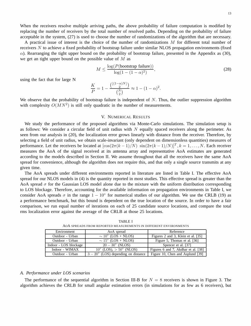
TABLE IAOA SPREADS FROM REPORTED MEASUREMENTS IN DIFFERENT ENVIRONMENTS

Environment AoA spread ReferenceOutdoor - Urban ∼ 10◦ (LOS + NLOS) Figures 2 and 3, Klein et al. [35]Outdoor - Urban ∼ 15◦ (LOS + NLOS) Figure 5, Thomas et al. [36]

Indoor - LOS blockage 20− 30◦ (NLOS) Spencer et al. [37]Indoor - WIMAX 10◦ (LOS), > 50◦ (NLOS) Figures 6 and 7, Akdhar et al. [38]Outdoor - Urban 3− 20◦ (LOS) depending on distance Figure 10, Chen and Asplund [39]

A. Performance under LOS scenarios

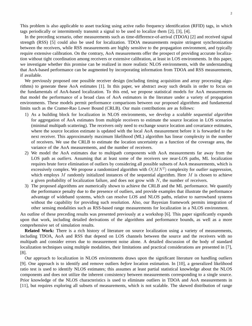
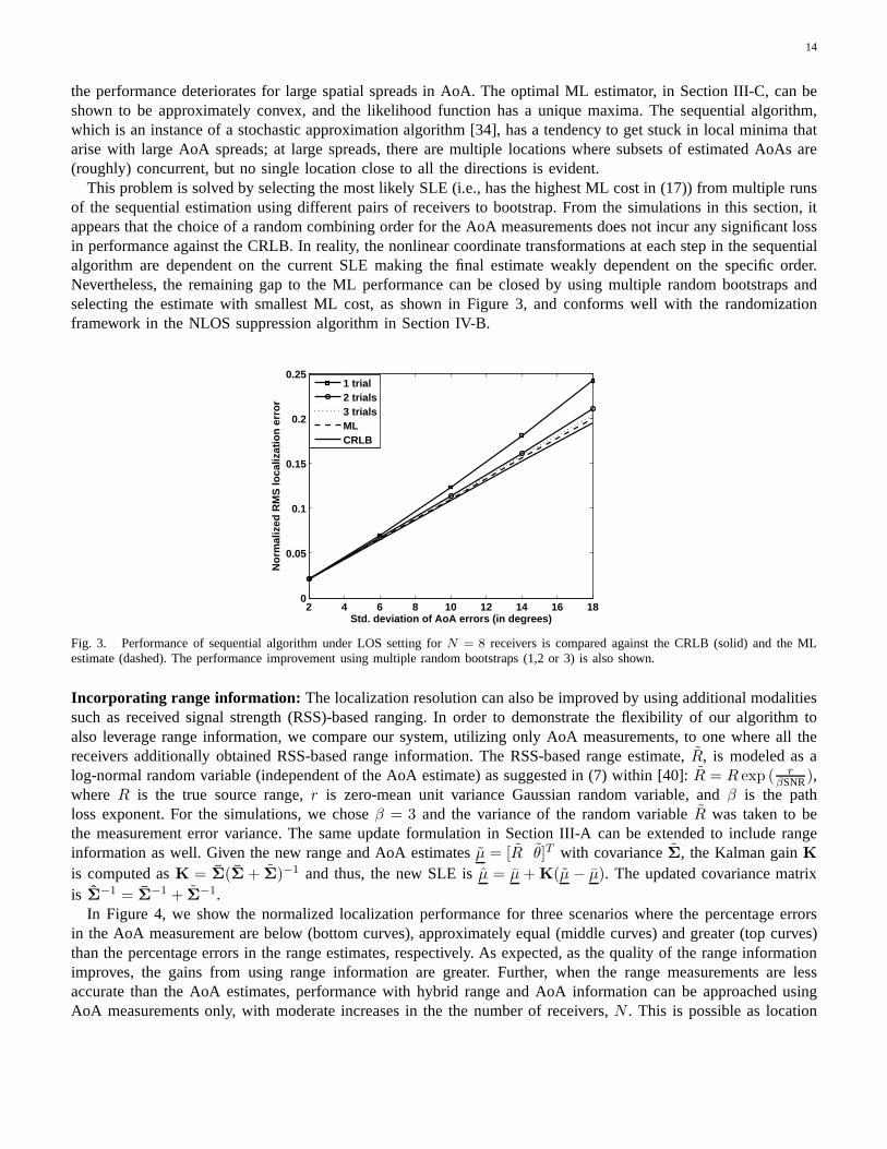
The performance of the sequential algorithm in Section III-B for N = 8 receivers is shown in Figure 3. Thealgorithm achieves the CRLB for small angular estimation errors (in simulations for as few as 6 receivers), but

14

the performance deteriorates for large spatial spreads in AoA. The optimal ML estimator, in Section III-C, can beshown to be approximately convex, and the likelihood function has a unique maxima. The sequential algorithm,which is an instance of a stochastic approximation algorithm [34], has a tendency to get stuck in local minima thatarise with large AoA spreads; at large spreads, there are multiple locations where subsets of estimated AoAs are(roughly) concurrent, but no single location close to all the directions is evident.

This problem is solved by selecting the most likely SLE (i.e., has the highest ML cost in (17)) from multiple runsof the sequential estimation using different pairs of receivers to bootstrap. From the simulations in this section, itappears that the choice of a random combining order for the AoA measurements does not incur any significant lossin performance against the CRLB. In reality, the nonlinear coordinate transformations at each step in the sequentialalgorithm are dependent on the current SLE making the final estimate weakly dependent on the specific order.Nevertheless, the remaining gap to the ML performance can beclosed by using multiple random bootstraps andselecting the estimate with smallest ML cost, as shown in Figure 3, and conforms well with the randomizationframework in the NLOS suppression algorithm in Section IV-B.

2 4 6 8 10 12 14 16 180

0.05

0.1

0.15

0.2

0.25

Std. deviation of AoA errors (in degrees)

Nor

mal

ized

RM

S lo

caliz

atio

n er

ror

1 trial2 trials3 trialsMLCRLB

Fig. 3. Performance of sequential algorithm under LOS setting for N = 8 receivers is compared against the CRLB (solid) and the MLestimate (dashed). The performance improvement using multiple random bootstraps (1,2 or 3) is also shown.

Incorporating range information: The localization resolution can also be improved by using additional modalitiessuch as received signal strength (RSS)-based ranging. In order to demonstrate the flexibility of our algorithm toalso leverage range information, we compare our system, utilizing only AoA measurements, to one where all thereceivers additionally obtained RSS-based range information. The RSS-based range estimate,R, is modeled as alog-normal random variable (independent of the AoA estimate) as suggested in (7) within [40]:R = R exp ( r

βSNR),where R is the true source range,r is zero-mean unit variance Gaussian random variable, andβ is the pathloss exponent. For the simulations, we choseβ = 3 and the variance of the random variableR was taken to bethe measurement error variance. The same update formulation in Section III-A can be extended to include rangeinformation as well. Given the new range and AoA estimatesµ = [R θ]T with covarianceΣ, the Kalman gainKis computed asK = Σ(Σ + Σ)−1 and thus, the new SLE isµ = µ +K(µ − µ). The updated covariance matrixis Σ

−1 = Σ−1 + Σ

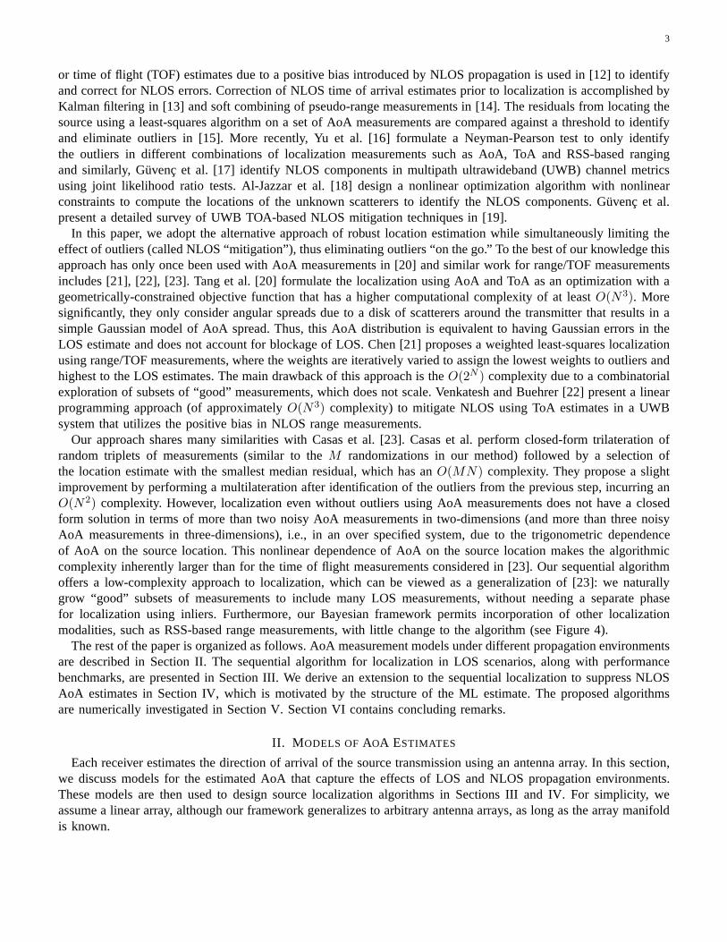
−1.In Figure 4, we show the normalized localization performance for three scenarios where the percentage errors

in the AoA measurement are below (bottom curves), approximately equal (middle curves) and greater (top curves)than the percentage errors in the range estimates, respectively. As expected, as the quality of the range informationimproves, the gains from using range information are greater. Further, when the range measurements are lessaccurate than the AoA estimates, performance with hybrid range and AoA information can be approached usingAoA measurements only, with moderate increases in the the number of receivers,N . This is possible as location

15

4 6 8 10 12 14 16 180

0.02

0.04

0.06

0.08

0.1

0.12

0.14

0.16

No. of receivers N

Nor

mal

ized

rm

s lo

caliz

atio

n er

ror

AoA + Range ( σ = 2ο)

AoA only ( σ = 2ο)

AoA + Range ( σ = 4ο)

AoA only ( σ = 4ο)

AoA + Range ( σ = 8ο)

AoA only ( σ = 8ο)

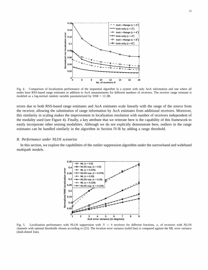
Fig. 4. Comparison of localization performance of the sequential algorithm in a system with only AoA information and onewhere allnodes have RSS-based range estimates in addition to AoA measurements for different numbers of receivers. The receiver range estimate ismodeled as a log-normal random variable parameterized by SNR = 12 dB.

errors due to both RSS-based range estimates and AoA estimates scale linearly with the range of the source fromthe receiver, allowing the substitution of range information by AoA estimates from additional receivers. Moreover,this similarity in scaling makes the improvement in localization resolution with number of receivers independent ofthe modality used (see Figure 4). Finally, a key attribute that we reiterate here is the capability of this framework toeasily incorporate other sensing modalities. Although we do not explicitly demonstrate here, outliers in the rangeestimates can be handled similarly in the algorithm in Section IV-B by adding a range threshold.

B. Performance under NLOS scenarios

In this section, we explore the capabilities of the outlier suppression algorithm under the narrowband and widebandmultipath models.

1 2 3 4 5 6 7 8 90

0.05

0.1

0.15

0.2

0.25

0.3

0.35

0.4

0.45

AoA error variance (in degrees)

Nor

mal

ized

RM

S lo

caliz

atio

n er

ror

ML (α = 0.5)NLOS sup. ( α = 0.5)ML (α = 0.375)NLOS sup. ( α = 0.375)ML (α = 0.25)NLOS sup. ( α = 0.25)ML (α = 0.125)NLOS sup. ( α = 0.125)

Fig. 5. Localization performance with NLOS suppression with N = 8 receivers for different fractions,α, of receivers with NLOSchannels with optimal thresholds chosen according to (25).The location error variance (solid line) is compared against the ML error variance(dash-dotted line).

16

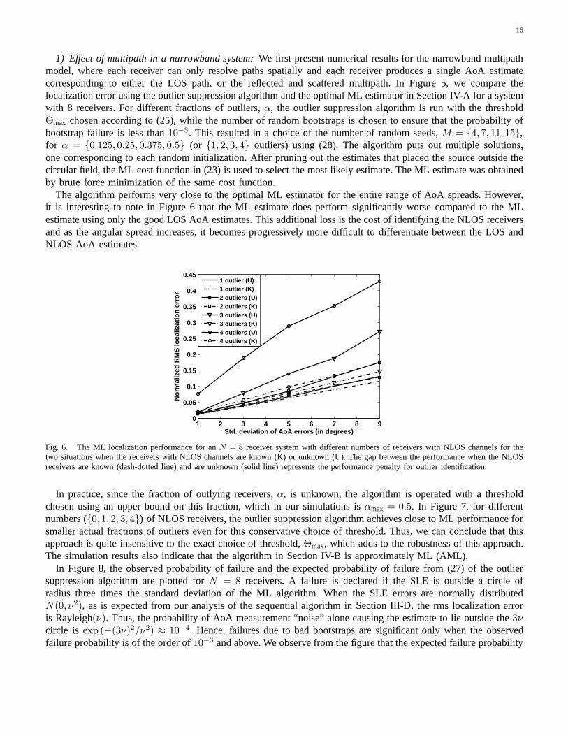
1) Effect of multipath in a narrowband system:We first present numerical results for the narrowband multipathmodel, where each receiver can only resolve paths spatiallyand each receiver produces a single AoA estimatecorresponding to either the LOS path, or the reflected and scattered multipath. In Figure 5, we compare thelocalization error using the outlier suppression algorithm and the optimal ML estimator in Section IV-A for a systemwith 8 receivers. For different fractions of outliers,α, the outlier suppression algorithm is run with the thresholdΘmax chosen according to (25), while the number of random bootstraps is chosen to ensure that the probability ofbootstrap failure is less than10−3. This resulted in a choice of the number of random seeds,M = {4, 7, 11, 15},for α = {0.125, 0.25, 0.375, 0.5} (or {1, 2, 3, 4} outliers) using (28). The algorithm puts out multiple solutions,one corresponding to each random initialization. After pruning out the estimates that placed the source outside thecircular field, the ML cost function in (23) is used to select the most likely estimate. The ML estimate was obtainedby brute force minimization of the same cost function.

The algorithm performs very close to the optimal ML estimator for the entire range of AoA spreads. However,it is interesting to note in Figure 6 that the ML estimate doesperform significantly worse compared to the MLestimate using only the good LOS AoA estimates. This additional loss is the cost of identifying the NLOS receiversand as the angular spread increases, it becomes progressively more difficult to differentiate between the LOS andNLOS AoA estimates.

1 2 3 4 5 6 7 8 90

0.05

0.1

0.15

0.2

0.25

0.3

0.35

0.4

0.45

Std. deviation of AoA errors (in degrees)

Nor

mal

ized

RM

S lo

caliz

atio

n er

ror

1 outlier (U)1 outlier (K)2 outliers (U)2 outliers (K)3 outliers (U)3 outliers (K)4 outliers (U)4 outliers (K)

Fig. 6. The ML localization performance for anN = 8 receiver system with different numbers of receivers with NLOS channels for thetwo situations when the receivers with NLOS channels are known (K) or unknown (U). The gap between the performance when the NLOSreceivers are known (dash-dotted line) and are unknown (solid line) represents the performance penalty for outlier identification.

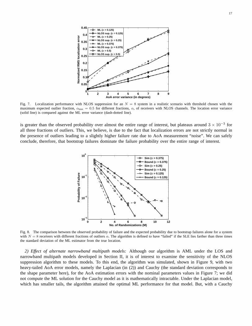
In practice, since the fraction of outlying receivers,α, is unknown, the algorithm is operated with a thresholdchosen using an upper bound on this fraction, which in our simulations isαmax = 0.5. In Figure 7, for differentnumbers ({0, 1, 2, 3, 4}) of NLOS receivers, the outlier suppression algorithm achieves close to ML performance forsmaller actual fractions of outliers even for this conservative choice of threshold. Thus, we can conclude that thisapproach is quite insensitive to the exact choice of threshold, Θmax, which adds to the robustness of this approach.The simulation results also indicate that the algorithm in Section IV-B is approximately ML (AML).

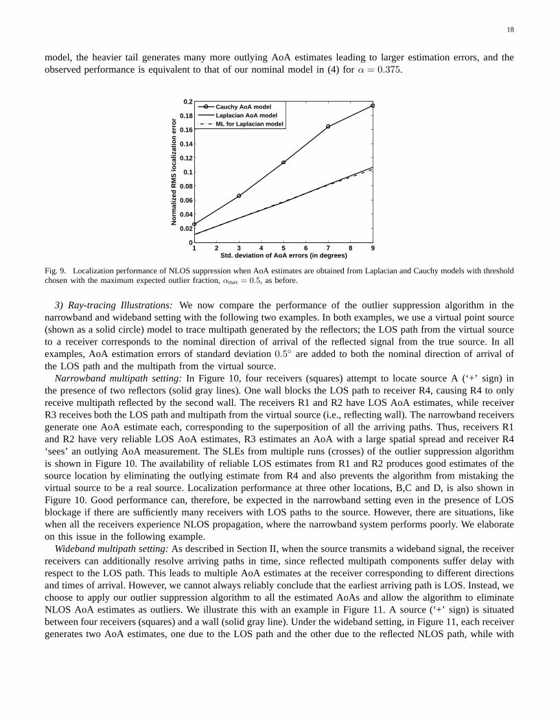
In Figure 8, the observed probability of failure and the expected probability of failure from (27) of the outliersuppression algorithm are plotted forN = 8 receivers. A failure is declared if the SLE is outside a circle ofradius three times the standard deviation of the ML algorithm. When the SLE errors are normally distributedN(0, ν2), as is expected from our analysis of the sequential algorithm in Section III-D, the rms localization erroris Rayleigh(ν). Thus, the probability of AoA measurement “noise” alone causing the estimate to lie outside the3νcircle is exp (−(3ν)2/ν2) ≈ 10−4. Hence, failures due to bad bootstraps are significant only when the observedfailure probability is of the order of10−3 and above. We observe from the figure that the expected failure probability

17

1 2 3 4 5 6 7 8 90

0.05

0.1

0.15

0.2

0.25

0.3

0.35

0.4

0.45

AoA error variance (in degrees)

Nor

mal

ized

RM

S lo

caliz

atio

n er

ror

ML (α = 0.125)NLOS sup. ( α = 0.125)ML (α = 0.25)NLOS sup. ( α = 0.25)ML (α = 0.375)NLOS sup. ( α = 0.375)ML (α = 0.5)NLOS sup. ( α = 0.5)

Fig. 7. Localization performance with NLOS suppression foran N = 8 system in a realistic scenario with threshold chosen with themaximum expected outlier fraction,αmax = 0.5 for different fractions,α, of receivers with NLOS channels. The location error variance(solid line) is compared against the ML error variance (dash-dotted line).

is greater than the observed probability over almost the entire range of interest, but plateaus around3 × 10−3 forall three fractions of outliers. This, we believe, is due to the fact that localization errors are not strictly normal inthe presence of outliers leading to a slightly higher failure rate due to AoA measurement “noise”. We can safelyconclude, therefore, that bootstrap failures dominate thefailure probability over the entire range of interest.

0 2 4 6 8 10 1210

−3

10−2

10−1

100

No. of Randomizations (M)

Pro

babi

lity

of F

ailu

re

Sim (α = 0.375)Bound ( α = 0.375)Sim (α = 0.25)Bound ( α = 0.25)Sim (α = 0.125)Bound ( α = 0.125)

Fig. 8. The comparison between the observed probability of failure and the expected probability due to bootstrap failures alone for a systemwith N = 8 receivers with different fractions of outliersα. The algorithm is defined to have “failed” if the SLE lies farther than three timesthe standard deviation of the ML estimator from the true location.

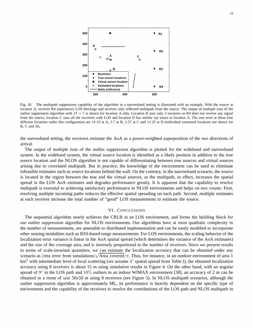
2) Effect of alternate narrowband multipath models:Although our algorithm is AML under the LOS andnarrowband multipath models developed in Section II, it is of interest to examine the sensitivity of the NLOSsuppression algorithm to these models. To this end, the algorithm was simulated, shown in Figure 9, with twoheavy-tailed AoA error models, namely the Laplacian (in (2)) and Cauchy (the standard deviation corresponds tothe shape parameter here), for the AoA estimation errors with the nominal parameters values in Figure 7; we didnot compute the ML solution for the Cauchy model as it is mathematically intractable. Under the Laplacian model,which has smaller tails, the algorithm attained the optimalML performance for that model. But, with a Cauchy

18

model, the heavier tail generates many more outlying AoA estimates leading to larger estimation errors, and theobserved performance is equivalent to that of our nominal model in (4) forα = 0.375.

1 2 3 4 5 6 7 8 90

0.02

0.04

0.06

0.08

0.1

0.12

0.14

0.16

0.18

0.2

Std. deviation of AoA errors (in degrees)

Nor

mal

ized

RM

S lo

caliz

atio

n er

ror

Cauchy AoA modelLaplacian AoA modelML for Laplacian model

Fig. 9. Localization performance of NLOS suppression when AoA estimates are obtained from Laplacian and Cauchy models with thresholdchosen with the maximum expected outlier fraction,αmax = 0.5, as before.

3) Ray-tracing Illustrations: We now compare the performance of the outlier suppression algorithm in thenarrowband and wideband setting with the following two examples. In both examples, we use a virtual point source(shown as a solid circle) model to trace multipath generatedby the reflectors; the LOS path from the virtual sourceto a receiver corresponds to the nominal direction of arrival of the reflected signal from the true source. In allexamples, AoA estimation errors of standard deviation0.5◦ are added to both the nominal direction of arrival ofthe LOS path and the multipath from the virtual source.

Narrowband multipath setting:In Figure 10, four receivers (squares) attempt to locate source A (‘+’ sign) inthe presence of two reflectors (solid gray lines). One wall blocks the LOS path to receiver R4, causing R4 to onlyreceive multipath reflected by the second wall. The receivers R1 and R2 have LOS AoA estimates, while receiverR3 receives both the LOS path and multipath from the virtual source (i.e., reflecting wall). The narrowband receiversgenerate one AoA estimate each, corresponding to the superposition of all the arriving paths. Thus, receivers R1and R2 have very reliable LOS AoA estimates, R3 estimates an AoA with a large spatial spread and receiver R4‘sees’ an outlying AoA measurement. The SLEs from multiple runs (crosses) of the outlier suppression algorithmis shown in Figure 10. The availability of reliable LOS estimates from R1 and R2 produces good estimates of thesource location by eliminating the outlying estimate from R4 and also prevents the algorithm from mistaking thevirtual source to be a real source. Localization performance at three other locations, B,C and D, is also shown inFigure 10. Good performance can, therefore, be expected in the narrowband setting even in the presence of LOSblockage if there are sufficiently many receivers with LOS paths to the source. However, there are situations, likewhen all the receivers experience NLOS propagation, where the narrowband system performs poorly. We elaborateon this issue in the following example.

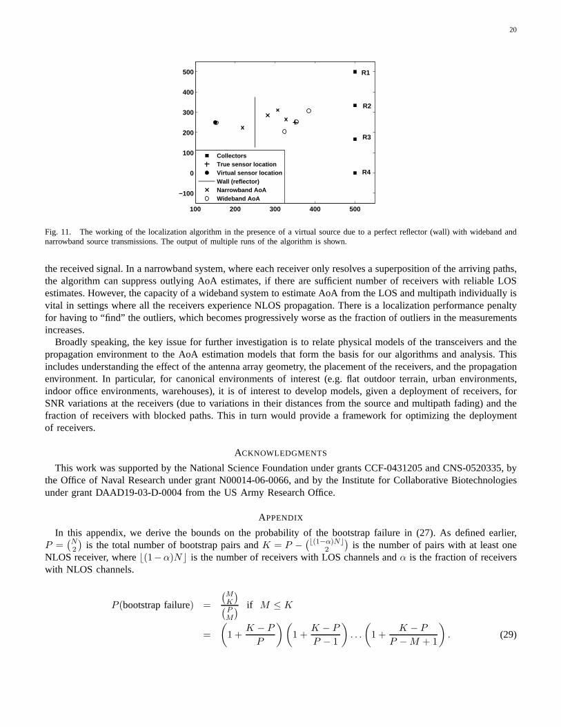
Wideband multipath setting:As described in Section II, when the source transmits a wideband signal, the receiverreceivers can additionally resolve arriving paths in time,since reflected multipath components suffer delay withrespect to the LOS path. This leads to multiple AoA estimatesat the receiver corresponding to different directionsand times of arrival. However, we cannot always reliably conclude that the earliest arriving path is LOS. Instead, wechoose to apply our outlier suppression algorithm to all theestimated AoAs and allow the algorithm to eliminateNLOS AoA estimates as outliers. We illustrate this with an example in Figure 11. A source (‘+’ sign) is situatedbetween four receivers (squares) and a wall (solid gray line). Under the wideband setting, in Figure 11, each receivergenerates two AoA estimates, one due to the LOS path and the other due to the reflected NLOS path, while with

19

300 400 500

0

100

200

300

400

500

ReceiversTrue sensor locationsVirtual sensor locationEstimated locationsWalls (reflectors)

R1

R2

CA

D

B R3

R4

Fig. 10. The multipath suppression capability of the algorithm in a narrowband setting is illustrated with an example. With the source atlocation A, receiver R4 experiences LOS blockage and receives only reflected multipath from the source. The output of multiple runs of theoutlier suppression algorithm withM = 7 is shown for location A only. Location B uses only 3 receiversas R4 does not receive any signalfrom the source, location C uses all the receivers with LOS and location D has similar ray traces to location A. The rms error at these fourdifferent locations under this configuration are18.42 at A, 2.7 at B, 2.57 at C and14.22 at D (individual estimated locations not shown forB, C and D).

the narrowband setting, the receivers estimate the AoA as a power-weighted superposition of the two directions ofarrival.

The output of multiple runs of the outlier suppression algorithm is plotted for the wideband and narrowbandsystem. In the wideband system, the virtual source locationis identified as a likely position in addition to the truesource location and the NLOS algorithm is not capable of differentiating between true sources and virtual sourcesarising due to correlated multipath. But in practice, the knowledge of the environment can be used to eliminateinfeasible estimates such as source locations behind the wall. On the contrary, in the narrowband scenario, the sourceis located in the region between the true and the virtual sources, as the multipath, in effect, increases the spatialspread in the LOS AoA estimates and degrades performance greatly. It is apparent that the capability to resolvemultipath is essential to achieving satisfactory performance in NLOS environments and helps on two counts: First,resolving multiple incoming paths reduces the effective spatial spreading on each path. Second, multiple estimatesat each receiver increase the total number of “good” LOS measurements to estimate the source.

VI. CONCLUSIONS

The sequential algorithm nearly achieves the CRLB in an LOS environment, and forms the building block forour outlier suppression algorithm for NLOS environments. Our algorithms have at most quadratic complexity inthe number of measurements, are amenable to distributed implementation and can be easily modified to incorporateother sensing modalities such as RSS-based range measurements. For LOS environments, the scaling behavior of thelocalization error variance is linear in the AoA spatial spread (which determines the variance of the AoA estimates)and the size of the coverage area, and is inversely proportional to the number of receivers. Since we present resultsin terms of scale-invariant quantities, we can estimate thelocalization accuracy that can be obtained under anyscenario as(rms error from simulations)

√Area covered/π. Thus, for instance, in an outdoor environment of area 1

km2 with intermediate level of local scattering (we assume4◦ spatial spread from Table I), the obtained localizationaccuracy using 8 receivers is about 15 m using simulation results in Figure 4. On the other hand, with an angularspread of9◦ in the LOS path and10% outliers in an indoor WIMAX environment [38], an accuracy of2 m can beobtained in a room of size 50x50 m using 8 receivers (see Figure 5). In NLOS multipath scenarios, although theoutlier suppression algorithm is approximately ML, its performance is heavily dependent on the specific type ofenvironment and the capability of the receivers to resolve the contributions of the LOS path and NLOS multipath in

20

100 200 300 400 500

−100

0

100

200

300

400

500

CollectorsTrue sensor locationVirtual sensor locationWall (reflector)Narrowband AoAWideband AoA

R1

R2

R3

R4

Fig. 11. The working of the localization algorithm in the presence of a virtual source due to a perfect reflector (wall) with wideband andnarrowband source transmissions. The output of multiple runs of the algorithm is shown.

the received signal. In a narrowband system, where each receiver only resolves a superposition of the arriving paths,the algorithm can suppress outlying AoA estimates, if thereare sufficient number of receivers with reliable LOSestimates. However, the capacity of a wideband system to estimate AoA from the LOS and multipath individually isvital in settings where all the receivers experience NLOS propagation. There is a localization performance penaltyfor having to “find” the outliers, which becomes progressively worse as the fraction of outliers in the measurementsincreases.

Broadly speaking, the key issue for further investigation is to relate physical models of the transceivers and thepropagation environment to the AoA estimation models that form the basis for our algorithms and analysis. Thisincludes understanding the effect of the antenna array geometry, the placement of the receivers, and the propagationenvironment. In particular, for canonical environments ofinterest (e.g. flat outdoor terrain, urban environments,indoor office environments, warehouses), it is of interest to develop models, given a deployment of receivers, forSNR variations at the receivers (due to variations in their distances from the source and multipath fading) and thefraction of receivers with blocked paths. This in turn wouldprovide a framework for optimizing the deploymentof receivers.

ACKNOWLEDGMENTS

This work was supported by the National Science Foundation under grants CCF-0431205 and CNS-0520335, bythe Office of Naval Research under grant N00014-06-0066, andby the Institute for Collaborative Biotechnologiesunder grant DAAD19-03-D-0004 from the US Army Research Office.

APPENDIX

In this appendix, we derive the bounds on the probability of the bootstrap failure in (27). As defined earlier,P =

(N2

)is the total number of bootstrap pairs andK = P −

(⌊(1−α)N⌋2

)is the number of pairs with at least one

NLOS receiver, where⌊(1−α)N⌋ is the number of receivers with LOS channels andα is the fraction of receiverswith NLOS channels.

P (bootstrap failure) =

(MK

)

(PM

) if M ≤ K

=

(

1 +K − P

P

)(

1 +K − P

P − 1

)

. . .

(

1 +K − P

P −M + 1

)

. (29)

21

In order to obtain an upper bound on the bootstrap failure probability, we replace each ratio of the formK−PP−k

bya larger fractionK−P

P(note thatK < P by definition):

P (bootstrap failure) ≤(K

P

)M

. (30)

Similarly, replacing the ratiosK−PP−k

by a smaller fraction K−PP−M+1 in (29), we get a lower bound,

P (bootstrap failure) ≥(K −M + 1

P −M + 1

)M

. (31)

The lower and upper bounds clearly converge ifM ≪ K < P , which occurs whenN is large. Moreover, thesebounds hold only forM ≤ K, as the probability of bootstrap failure is zero ifM > K.

REFERENCES

[1] B. Ananthasubramaniam and U. Madhow, “Collector receiver design for data collection and localization in sensor-driven networks,” inProc. Conference on Information Sciences and Systems, 2007., 2007, pp. 591–596.

[2] “Aeroscout inc.” [Online]. Available: http://www.aeroscout.com/[3] “Savi technology inc.” [Online]. Available: http://www.savi.com/index.shtml[4] “Wherenet inc.” [Online]. Available: http://www.wherenet.com/[5] “Ekahau inc.” [Online]. Available: http://www.ekahau.com/[6] B. Ananthasubramaniam and U. Madhow, “Cooperative localization using angle of arrival measurements in non-line-of-sight

environments,” inMELT ’08: Proc. ACM international workshop on Mobile entitylocalization and tracking in GPS-less environments,San Francisco, CA, Sept. 2008, pp. 117–122.

[7] N. Patwari, J. Ash, S. Kyperountas, A. Hero, R. Moses, andN. Correal, “Locating the nodes: cooperative localizationin wireless sensornetworks,” IEEE Signal Process. Mag., vol. 22, no. 4, pp. 54–69, 2005.

[8] G. Mao, B. Fidan, and B. D. Anderson, “Wireless sensor network localization techniques,”Computer Networks, vol. 51, no. 10, pp.2529–2553, Jul. 2007.

[9] R. A. Maronna, D. R. Martin, and V. J. Yohai,Robust Statistics: Theory and Methods. Wiley, 2006.[10] J. Borras, P. Hatrack, and N. Mandayam, “A decision theoretic framework for NLOS identification,” inProc. VTC’98, vol. 2, May

1998, pp. 1583–1587.[11] L. Cong and W. Zhuang, “Nonline-of-sight error mitigation in mobile location,”IEEE Trans. Wireless Commun., vol. 4, no. 2, pp.

560–573, 2005.[12] S. Venkatraman and J. Caffery Jr, “Statistical approach to nonline-of-sight BS identification,” inProc. WPMC’02, vol. 1, Honolulu,

Hawaii, Oct 2002, pp. 296–300.[13] B. L. Le, K. Ahmed, and H. Tsuji, “Mobile location estimator with NLOS mitigation using kalman filtering,” inProc. WCN’03, vol. 3,

Mar. 2003, pp. 1969–1973.[14] S. Srirangarajan and A. H. Tewfik, “Sensor node localization via spatial domain quasi-maximum likelihood estimation,” in Proc.

EUSIPCO’06, 2006. [Online]. Available: http://www.arehna.di.uoa.gr/Eusipco2006/papers/1568979916.pdf[15] L. Xiong, “A selective model to suppress NLOS signals inangle-of-arrival (AOA) location estimation,” inProc. PIMRC’98, vol. 1,

Sept. 1998, pp. 461–465.[16] K. Yu and Y. Guo, “Statistical NLOS identification basedon AOA, TOA, and signal strength,”IEEE Trans. Veh. Technol., vol. 58,

no. 1, pp. 274–286, 2009.[17] I. Guvenc, C.-C. Chong, F. Watanabe, and H. Inamura, “NLOS identification and weighted least-squares localization for UWB systems

using multipath channel statistics,”EURASIP Journal on Advances in Signal Processing, vol. 2008, p. 14, 2008, article ID 271984,doi: 10.1155/2008/271984.

[18] S. Al-Jazzar, M. Ghogho, and D. McLernon, “A joint TOA/AOA constrained minimization method for locating wireless devices innon-line-of-sight environment,”IEEE Trans. Veh. Technol., vol. 58, no. 1, pp. 468–472, 2009.

[19] I. Guvenc and C.-C. Chong, “A survey on TOA based wireless localization and NLOS mitigation techniques,”IEEE Commun. SurveysTuts., 2009, to appear.

[20] H. Tang, Y. Park, and T. Qiu, “A TOA-AOA-based NLOS errormitigation method for location estimation,”EURASIP Journal onAdvances in Signal Processing, vol. 2008, p. 14, 2008, article ID 682528, doi:10.1155/2008/682528.

[21] P. C. Chen, “A non-line-of-sight error mitigation algorithm in location estimation,” inProc. WCNC’99, Sept. 1999, pp. 316–320.[22] S. Venkatesh and R. Buehrer, “NLOS mitigation using linear programming in ultrawideband location-aware networks,” IEEE Trans.

Veh. Technol., vol. 56, no. 5, pp. 3182–3198, 2007.[23] R. Casas, A. Marco, J. J. Guerrero, and J. Falco, “Robust estimator for non-line-of-sight error mitigation in indoor localization,”

EURASIP Journal on Applied Signal Processing, vol. 2006, p. 8, 2006, doi:10.1155/ASP/2006/43429.[24] L. C. Godara, “Application of antenna arrays to mobile communications. II. beam-forming and direction-of-arrival considerations,”

Proc. IEEE, vol. 85, no. 8, pp. 1195–1245, Aug 1997.

22

[25] R. Raich, J. Goldberg, and H. Messer, “Bearing estimation for a distributed source: Modeling, inherent accuracy limitations, andalgorithms,” IEEE Trans. Signal Process., vol. 48, pp. 429–441, Feb. 2000.

[26] R. B. Ertel, K. Sowerby, T. S. Rappaport, and J. H. Reed, “Overview of spatial channel models for antenna array communicationsystems,”IEEE Personal Commun. Mag., pp. 10–22, 1998.

[27] Y. Meng, P. Stoica, and K. M.Wong, “Estimation of the directions of arrival of spatially dispersed signals in array processing,”IEEProceedings Radar, Sonar and Navigation, vol. 143, no. 1, pp. 1–9, Feb. 1996.

[28] T. Trump and B. Ottersten, “Estimation of nominal direction of arrival and angular spread using an array of sensors,” Signal Processing,vol. 50, no. 1-2, pp. 57–69, 1996.

[29] S. Valaee, B. Champagne, and P. Kabal, “Parametric localization of distributed sources,”IEEE Trans. Signal Process., vol. 43, no. 9,pp. 2144–2153, Sept. 1995.

[30] Q. H. Spencer, B. D. Jeffs, M. A. Jensen, and A. L. Swindlehurst, “Modeling the statistical time and angle of arrival characteristics ofan indoor multipath channel,”IEEE J. Sel. Areas Commun., vol. 18, no. 3, pp. 347–360, Mar. 2000.

[31] B. Rao and K. Hari, “Performance analysis of root-music,” IEEE Trans. Signal Process., vol. 37, no. 12, pp. 1939–1949, Dec 1989.[32] B. W. Parkinson and J. J. Spilker,Global Positioning System: Theory and Practice. American Institute of Aeronautics, 1996.[33] T. F. Coleman and Y. Li, “An interior trust region approach for nonlinear minimization subject to bounds,”SIAM Journal on Optimization,

vol. 6, no. 2, pp. 418–445, 1996.[34] H. V. Poor,An Introduction to Signal Detection and Estimation, 2nd ed. Springer, 2005.[35] A. Klein, W. Mohr, R. Thomas, P. Weber, and B. Wirth, “Direction-of-arrival of partial waves in wideband mobile radio channels for

intelligent antenna concepts,” inProc. VTC, vol. 2, 1996, pp. 849–853.[36] H. J. Thomas, T. Ohgane, and M. Mizuno, “A novel dual antenna measurement of the angular distribution of received waves in the

mobile radio environment as a function of position and delaytime,” in Proc. VTC, vol. 1, 1992, pp. 546–549.[37] Q. Spencer, M. Rice, B. Jeffs, and M. Jensen, “Indoor wideband time/angle of arrival multipath propagation results,” in Proc. VTC,

vol. 3, 1997, pp. 1410–1414.[38] O. Akhdar, D. Carsenat, C. Decroze, M. Mouhamadou, and T. Monediere, “Direction of arrival measurements for outdoor-to- indoor

channel characterization,” inProc. EuCAP 2009, Mar. 2009, pp. 2280–2282.[39] M. Chen and H. Asplund, “Measurements and models for direction of arrival of radio waves in los in urban microcells,”in Proc.

PIMRC, vol. 1, 2001, pp. B–100– B–104.[40] N. Patwari, I. Hero, A.O., M. Perkins, N. Correal, and R.O’Dea, “Relative location estimation in wireless sensor networks,” IEEE

Trans. Signal Process., vol. 51, no. 8, pp. 2137–2148, Aug. 2003.