6DoF Cooperative Localization for Mutually Observing Robotspgiguere/papers/isrr2013.pdf · 6DoF Cooperative Localization for Mutually Observing Robots 3 The accuracy of vision-based

6DoF Cooperative Localization for MutuallyObserving Robots

Olivier Dugas, Philippe Giguere and Ioannis Rekleitis

Abstract The solution of cooperative localization is of particular importance toteams of aerial or underwater robots operating in areas devoid of landmarks. Theproblem becomes harder if the localization system must be low-cost and lightweightenough that only consumer-grade cameras can be used. This paper presents an an-alytical solution to the six degrees of freedom cooperative localization problem us-ing bearing only measurements. Given two mutually observing robots, each oneequipped with a camera and two markers, and given that they each take a picture atthe same moment, we can recover the coordinate transformation that expresses thepose of one robot in the frame of reference of the other. The novelty of our approachis the use of two pairs of bearing measurements for the pose estimation instead ofusing both bearing and range measurements. The accuracy of the results is verifiedin extensive simulations and in experiments with real hardware. At 6.5 m distance,position was estimated with a mean error between 0.021 m and 0.025 m and orienta-tion was recovered with a mean error between 0.019 rad and 0.037 rad. This makesour solution particularly well suited for deployment on fleets of inexpensive robotsmoving in 6 DoF such as blimps.

1 Introduction

In GPS-denied environment, such as underground, underwater, or indoors, espe-cially when features are sparse, the problem of localizing a team of robots can beaddressed by the employment of the Cooperative Localization (CL) [22] methodol-ogy. In CL, robots use observations of each other in order to calculate their relativepose (position and orientation) without resorting to measuring features in the envi-ronment. The vast majority of research on CL has focused on the 2D case, with the

Olivier Dugas and Philippe GiguereDepartement d’informatique et de genie logiciel, Universite Laval, 3976-1065 Avenuede la Medecine, Quebec, QC, Canada G1V 0A6. e-mail: [email protected]@ulaval.ca

Ioannis RekleitisSchool of Computer Science, McGill University, 318-3480 University Street, Montreal, QC,Canada H3A 2A7 e-mail: [email protected]

1

2 Olivier Dugas, Philippe Giguere and Ioannis Rekleitis

advent of more advanced mobile robots such as aerial, underwater or even roughterrain (outdoor) robots, the problem of estimating the relative pose in 3D is gain-ing popularity. Even when GPS is available, its accuracy in estimating the pose isinsufficient for precise maneuvering, as compared to CL solutions.

More formally, for a team of robots, Cooperative Localization can be defined asfollows: given a set of inter-robot measurements, estimate the relative pose of eachrobot with respect to the other team members. If one robot is stationary, then thepose of the other team members can be defined with respect to the stationary robot.

In this paper, we present an analytical solution for the 3D transformation thatdescribes the relative pose between two robots, using a limited number of bear-ing measurements. We show how one can use the angle measurements obtained bycameras to estimate the relative 3D position and orientation of mutually observingrobots. In the following section, an overview of related work is provided. Section3 describes the 3D problem we are addressing, along with the proposed analyti-cal solution. Section 4 presents the tracking experiment setup and Section 5 showsthe results. Thereafter, Section 6 investigates the effects of a non-collinear camera-markers setup on the solution. Finally, we conclude with future directions for thiswork, and lessons learned.

2 Previous Work

Estimating the relative pose of a group of robots was presented as early as 1994 [18].Early work focused on 2D pose estimation for localization [17] and mapping [20]using either a Kalman [23] or a Particle [21] filter. An interesting variation appearswhen the measurements do not come from identifiable robots (anonymous) [10].More recently, work on using bearing only measurements produced an accurate so-lution for the 2D case [12]. It is worth mentioning that using bearing only measure-ments from a camera is an inexpensive solution which scales to large number ofrobots.

Employing Cooperative Localization to derive the 6-DoF relative pose measure-ments has gained popularity lately. In an application to the underwater domain, Bahret. al. used a 2D approximation [1] by maintaining the same depth. The anony-mous measurement solution to CL was extended in [3] using relative bearings andinertial data. The main contribution on this work is the data association, whichis achieved by the additional ego-motion sensor data. Zhou and Roumeliotis pre-sented a extensive list of solutions for Cooperative Localization in 3D using com-binations of range and bearing measurements in conjunction with ego-motion mea-surements [28, 29, 30]. Contrary to our solution, a single bearing measurement isrecorded each time from each robot, making the use of proprioceptive sensors a re-quirement. Cristofaro and Martinelli [4] presented an observability analysis for astate estimation system using bearing measurements and inertial data. In their for-mulation, the inertial data is necessary to recover the full pose. The reader will notethat the observability analysis can be used to improve the EKF-based estimators inCL [13].

6DoF Cooperative Localization for Mutually Observing Robots 3

The accuracy of vision-based systems for distance measurements is limited,mainly due to discretization errors. However, many techniques have been devel-oped to improve the precision using bearing measurements, since cameras are goodprotractors. For instance, bearing measurements were used in [27] to estimate theconfiguration parameters of a continuum robot. Also, implicit localization methodswere presented with bearing-only measurements in [15] and [7] showed that rel-ative measurements localization can be an NP-hard problem. Polynomial solverswere developed and optimized for solving minimal geometry problems [19]. In [6]a numerical solution was proposed for estimating the 3D relative pose using bearingonly measurements. The accuracy of the reported results are lower than the onesobtained from the analytical solution proposed in this paper.

One of the oldest minimal geometry problem in computer vision is known as thePerspective-n-Point (PnP) problem. It is defined as the determination of the abso-lute pose of a camera given a set of correspondences between 3D points and theirprojections on the 2D image taken by the camera. Closed-form solutions have beenproposed to the minimal absolute pose problems with known vertical direction [16]and also to the three points absolute pose problem [9].

Other vision-based approaches used different sensors to provide the bearing of anobserved robot. Omni-directional cameras were used in [14] and [11]. Also, bearingand distance estimations were provided using active lighting with stereo vision in[5] or by combining vision with range finders in [2]. Relative bearing and/or rangemeasurements has been employed in a constraint optimization framework [26]. Oursolution, however, differentiates itself by the fact that only three to four angles andno distance estimation are needed to estimate the pose of an observed robot.

3 Solution to the 3D Problem

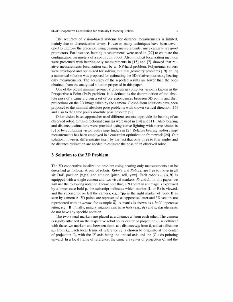
The 3D cooperative localization problem using bearing only measurements can bedescribed as follows. A pair of robots, RobotA and RobotB, are free to move in allsix DoF, position [x,y,z] and attitude [pitch, roll, yaw]. Each robot i ∈ {A,B} isequipped with a single camera and two visual markers, Ri and Li. In this paper, wewill use the following notation. Please note that, a 2D point in an image is expressedby a lower case bold p, the subscript indicates which marker (L or R) is viewed,and the superscript on left the camera, e.g.: ApR is the right marker of robot B asseen by camera A. 3D points are represented as uppercase letter and 3D vectors arerepresented with an arrow, for example

−→Ri . A matrix is shown as a bold uppercase

letter, e.g.: R. Finally, unitary rotation axis have hats (e.g.: e1) and scalar elementsdo not have any specific notation.

The two visual markers are placed at a distance d from each other. The camerais rigidly attached on the respective robot so its center of projection Ci is collinearwith these two markers and between them, at a distance dRi from Ri and at a distancedLi from Li. Each local frame of reference Fi is chosen to originate at the centerof projection Ci, with the −→z axis being the optical axis and the −→y axis pointingupward. In a local frame of reference, the camera’s center of projection Ci and the


Fig. 1 The relative localization problem in 3D, for the two robots A and B operating in 6 DoF.In this depiction, we only show the markers on robot A. The red and green lines represent the raybetween these markers and the center of projection of CameraB, located at the origin of FB.

two markers are thus located at:

Ci = [0 0 0], Ri = [−dRi 0 0], Li = [dLi 0 0].

Please note that the x coordinate for the right marker Ri is negative, as per the ori-entation of the frame of reference Fi; see Fig. 1. Finally, we assume that at all time,each camera can see the other robot and its two landmarks.

The relative pose between RobotA and RobotB is calculated by using two imagesrecorded at the same time. Let the picture taken by RobotA be IA, and the picturetaken by RobotB be IB. Each robot i, along with its two markers Ri and Li, is presentin the image acquired by the other robot, i.e. RB and LB appear in IA and vice versa.This situation is illustrated in Fig. 1. The relative orientation and position betweenFA and FB will be expressed as a translation matrix A

BT and a rotation matrix ABR. The

information available to find this transformation is:

• the position of the markers Ri = [−dRi 0 0] and Li = [dLi 0 0] within their robot’sframe of reference Fi;

• the camera calibration internal parameters;• sub-pixel location ApR and ApL in image IA of RB and LB, respectively;• sub-pixel location BpR and BpL in image IB of RA and LA, respectively.

From the above information, we can also infer the approximate position of the otherrobot’s camera in an image, given that it is located by construction between the twomarkers:

• sub-pixel location in image IA of CB as

ApB ≈ ApR +

(dRB

dLB +dRB

)(ApL− ApR); (1)


• and sub-pixel location in image IB of CA:

BpA ≈ BpR +

(dRA

dLA +dRA

)(BpL− BpR). (2)

This approximation holds when the robots are sufficiently far apart (l� d) or whenthe robots are perfectly facing each other. Please note that ipX indicates the positionof point X (camera, or marker R or L), in the frame of reference of i.

3.1 Reduction to 2D problem

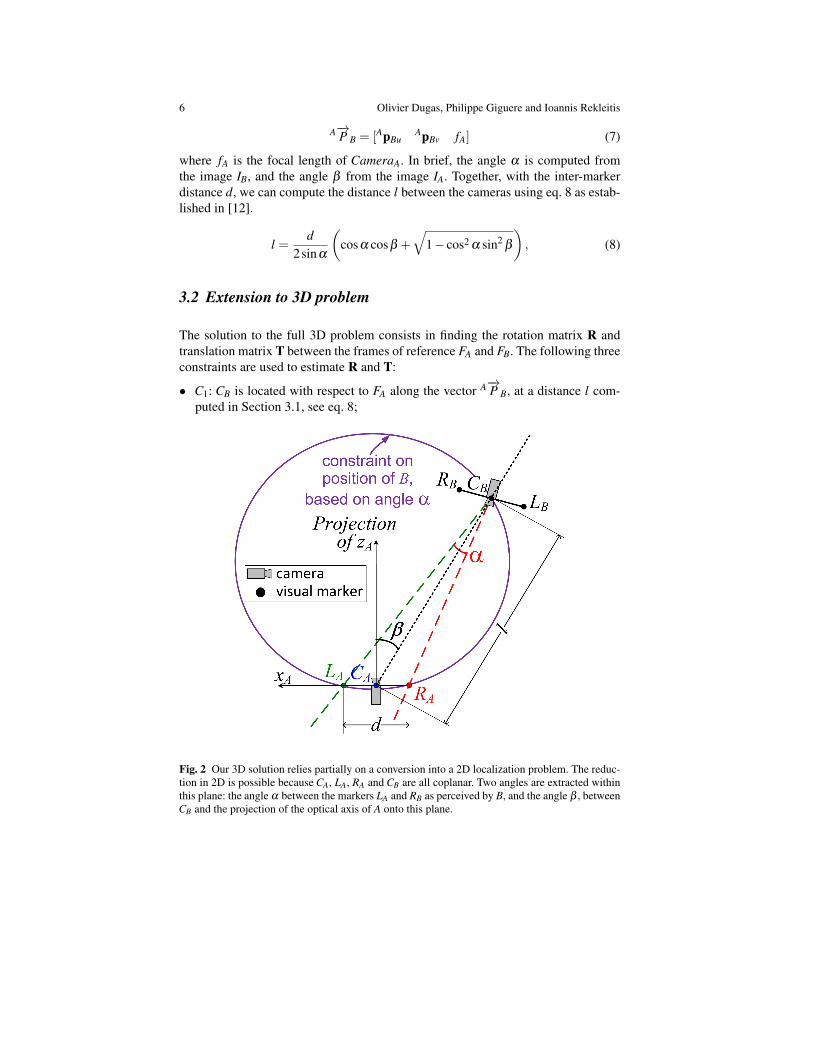
Let us first consider the plane defined in 3D space by the three collinear points (byphysical construction) RA, LA, CA on robot A and the center of the camera on robotB, point CB. Note that the origins of the two frames of reference FA and FB are alsopart of this plane, since the origin of frame Fi is defined as the center of projectionCi of a camera. This is the key to our solution, as it allows to reduce part of the 3Dcalculation into a 2D problem, the solution of the reduced problem being identicalto the one presented in [12] and depicted in Fig. 2. In particular, the 2D solutionestimates the distance between the two cameras l = |CACB|.

As described in [12], the estimation of the relative position requires the measure-ment of two angles, α and β and knowing the distance d between the markers LA

and RA. In the current formulation, the angle LACBRA = α is defined within thatplane and is computed straightforward by creating the 3D vectors going from theorigin to the image plane of IB

B−→P R = [B pRuB pRv fB] (3)

andB−→P L = [B pLu

B pLv fB] (4)

where fB is the focal length of CameraB. Note that the subscripts u, v indicate thehorizontal and vertical pixel location in an image. The angle α is then the anglebetween these two vectors, computed as:

α = acos(B−→P L ·B

−→P R

|B−→P L||B−→P R|

) (5)

The angle β , using the projection of the optical axis −→z onto that plane, is com-puted from IA by noting that the vector

−−−→CARA in FA is necessarily perpendicular to

this projection. From the above follows:

β =π

2−acos(

A−→P B ·−−−→CARA

|A−→P B||−−−→CARA|

), (6)

with


A−→P B = [ApBuApBv fA] (7)

where fA is the focal length of CameraA. In brief, the angle α is computed fromthe image IB, and the angle β from the image IA. Together, with the inter-markerdistance d, we can compute the distance l between the cameras using eq. 8 as estab-lished in [12].

l =d

2sinα

(cosα cosβ +

√1− cos2 α sin2

β

), (8)

3.2 Extension to 3D problem

The solution to the full 3D problem consists in finding the rotation matrix R andtranslation matrix T between the frames of reference FA and FB. The following threeconstraints are used to estimate R and T:

• C1: CB is located with respect to FA along the vector A−→P B, at a distance l com-puted in Section 3.1, see eq. 8;

Fig. 2 Our 3D solution relies partially on a conversion into a 2D localization problem. The reduc-tion in 2D is possible because CA, LA, RA and CB are all coplanar. Two angles are extracted withinthis plane: the angle α between the markers LA and RB as perceived by B, and the angle β , betweenCB and the projection of the optical axis of A onto this plane.


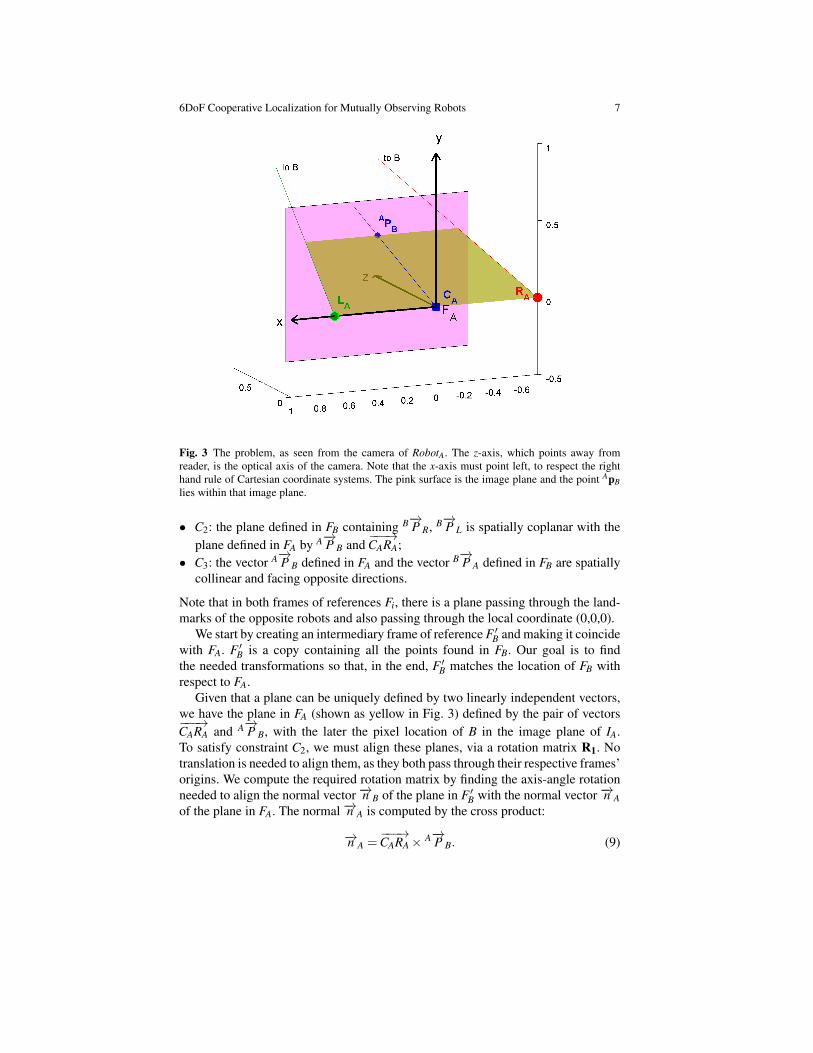
Fig. 3 The problem, as seen from the camera of RobotA. The z-axis, which points away fromreader, is the optical axis of the camera. Note that the x-axis must point left, to respect the righthand rule of Cartesian coordinate systems. The pink surface is the image plane and the point ApBlies within that image plane.

• C2: the plane defined in FB containing B−→P R, B−→P L is spatially coplanar with theplane defined in FA by A−→P B and

−−−→CARA;

• C3: the vector A−→P B defined in FA and the vector B−→P A defined in FB are spatiallycollinear and facing opposite directions.

Note that in both frames of references Fi, there is a plane passing through the land-marks of the opposite robots and also passing through the local coordinate (0,0,0).

We start by creating an intermediary frame of reference F ′B and making it coincidewith FA. F ′B is a copy containing all the points found in FB. Our goal is to findthe needed transformations so that, in the end, F ′B matches the location of FB withrespect to FA.

Given that a plane can be uniquely defined by two linearly independent vectors,we have the plane in FA (shown as yellow in Fig. 3) defined by the pair of vectors−−−→CARA and A−→P B, with the later the pixel location of B in the image plane of IA.To satisfy constraint C2, we must align these planes, via a rotation matrix R1. Notranslation is needed to align them, as they both pass through their respective frames’origins. We compute the required rotation matrix by finding the axis-angle rotationneeded to align the normal vector −→n B of the plane in F ′B with the normal vector −→n Aof the plane in FA. The normal −→n A is computed by the cross product:

−→n A =−−−→CARA× A−→P B. (9)


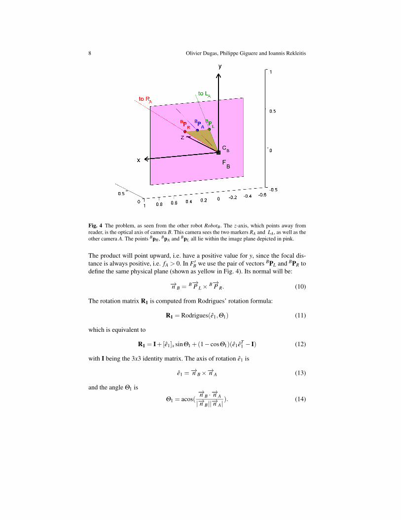
Fig. 4 The problem, as seen from the other robot RobotB. The z-axis, which points away fromreader, is the optical axis of camera B. This camera sees the two markers RA and LA, as well as theother camera A. The points BpR, BpA and BpL all lie within the image plane depicted in pink.

The product will point upward, i.e. have a positive value for y, since the focal dis-tance is always positive, i.e. fA > 0. In F ′B we use the pair of vectors BPL and BPR todefine the same physical plane (shown as yellow in Fig. 4). Its normal will be:

−→n B = B−→P L× B−→P R. (10)

The rotation matrix R1 is computed from Rodrigues’ rotation formula:

R1 = Rodrigues(e1,Θ1) (11)

which is equivalent to

R1 = I+[e1]x sinΘ1 +(1− cosΘ1)(e1eT1 − I) (12)

with I being the 3x3 identity matrix. The axis of rotation e1 is

e1 =−→n B×−→n A (13)

and the angle Θ1 is

Θ1 = acos(−→n B ·−→n A

|−→n B||−→n A|). (14)


With FA and R1F ′B having their planes coplanar, the next step is to align the vectorR1

B−→P A with the opposite vector−A−→P B with a rotation matrix R2, in order to satisfyconstraint C3. This rotation happens in the same plane defined earlier, so the rotationaxis is e2 =

−→n A. The angle of rotation is calculated as follows:

Θ2 = acos(−A−→P B ·R1

B−→P A

|A−→P B||B−→P A|

) = π− acos(A−→P B ·R1

B−→P A

|A−→P B||B−→P A|

). (15)

The second rotation matrix will be:

R2 = Rodrigues(e2,Θ2). (16)

Finally, we translate R2R1F ′B by the distance l, along the A−→P B axis to meet theconstraint C1:

−→T = l

A−→P B

|A−→P B|, (17)

with−→T being trivially convertible to the translation matrix, T. We thus have found

the transformation between frames FA and FB, and hence the relative pose estimate,since

AFB = TR2R1F ′B, (18)

with the position and orientation of FB expressed in FA’s coordinate is AFB, and thetransformed F ′B coincide with AFB at this point.

To verify the correctness of the above formulae, we implemented a simulation inMATLAB. The algorithm was able to recover the position and orientation of RobotBrelative to RobotA. We also investigated the estimation of ApB and BpA in equations1 and 2, which impacts the evaluation of β . The error on β was less than a tenthof a percent of the real β value at a distance of about 10 m, which resulted in anadditional mean position and orientation errors of 0.57 cm and 0.05 deg, respec-tively. A discussion on noise models and their impact on real world applications isavailable in [12], which still apply to our 3D extension of the analytical solution viathe distance l.

4 Experimental Setup

Two identical assemblies were constructed, each one comprising of a consumer-grade Logitech C905 camera and two white LEDs 1 as markers. The camera and themarkers were securely fixed on an aluminum rod. The camera had a 75o diagonalfield of view and the LEDs had a viewing angle of 140o. The distance between themarkers were dA = 83.1 cm and dB = 75.7 cm. The optical axis of the camera wasperpendicular to the rod. The rig A was placed on a table and used as the fixed frameof reference FA.

1 LED model SMP6-UWDW (4000 micro-candelas) from Bivar Inc


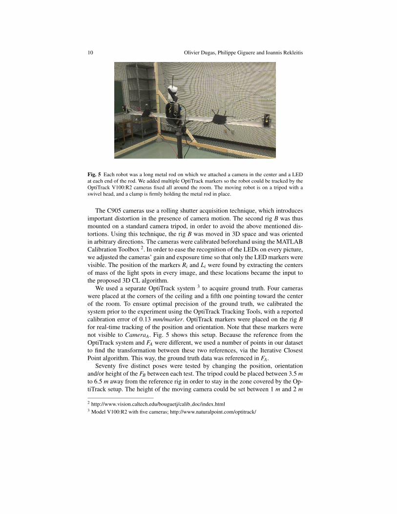
Fig. 5 Each robot was a long metal rod on which we attached a camera in the center and a LEDat each end of the rod. We added multiple OptiTrack markers so the robot could be tracked by theOptiTrack V100:R2 cameras fixed all around the room. The moving robot is on a tripod with aswivel head, and a clamp is firmly holding the metal rod in place.

The C905 cameras use a rolling shutter acquisition technique, which introducesimportant distortion in the presence of camera motion. The second rig B was thusmounted on a standard camera tripod, in order to avoid the above mentioned dis-tortions. Using this technique, the rig B was moved in 3D space and was orientedin arbitrary directions. The cameras were calibrated beforehand using the MATLABCalibration Toolbox 2. In order to ease the recognition of the LEDs on every picture,we adjusted the cameras’ gain and exposure time so that only the LED markers werevisible. The position of the markers Ri and Li were found by extracting the centersof mass of the light spots in every image, and these locations became the input tothe proposed 3D CL algorithm.

We used a separate OptiTrack system 3 to acquire ground truth. Four cameraswere placed at the corners of the ceiling and a fifth one pointing toward the centerof the room. To ensure optimal precision of the ground truth, we calibrated thesystem prior to the experiment using the OptiTrack Tracking Tools, with a reportedcalibration error of 0.13 mm/marker. OptiTrack markers were placed on the rig Bfor real-time tracking of the position and orientation. Note that these markers werenot visible to CameraA. Fig. 5 shows this setup. Because the reference from theOptiTrack system and FA were different, we used a number of points in our datasetto find the transformation between these two references, via the Iterative ClosestPoint algorithm. This way, the ground truth data was referenced in FA.

Seventy five distinct poses were tested by changing the position, orientationand/or height of the FB between each test. The tripod could be placed between 3.5 mto 6.5 m away from the reference rig in order to stay in the zone covered by the Op-tiTrack setup. The height of the moving camera could be set between 1 m and 2 m

2 http://www.vision.caltech.edu/bouguetj/calib doc/index.html3 Model V100:R2 with five cameras; http://www.naturalpoint.com/optitrack/


off the ground. Lateral movements could not be over 3 m away from the center ofthe images taken by the reference camera, or else we would have placed CameraBoutside the OptiTrack system’s covering area.

5 Experimental Results

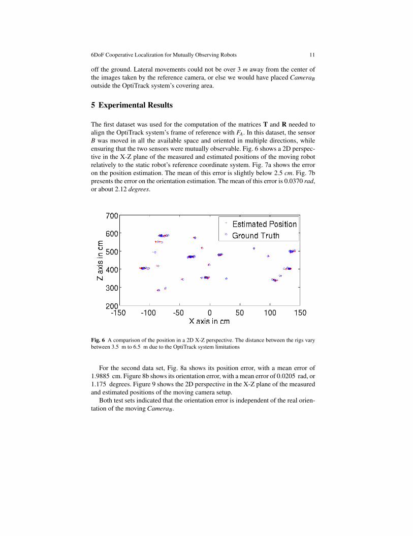
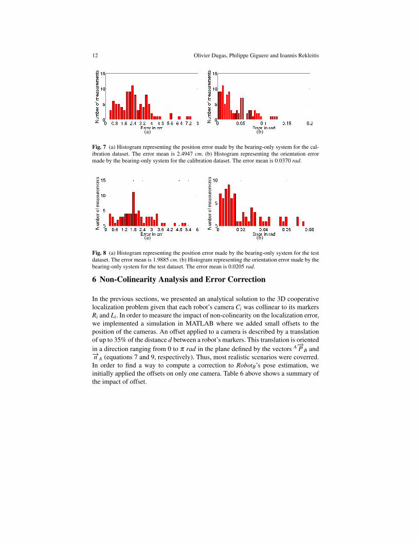
The first dataset was used for the computation of the matrices T and R needed toalign the OptiTrack system’s frame of reference with FA. In this dataset, the sensorB was moved in all the available space and oriented in multiple directions, whileensuring that the two sensors were mutually observable. Fig. 6 shows a 2D perspec-tive in the X-Z plane of the measured and estimated positions of the moving robotrelatively to the static robot’s reference coordinate system. Fig. 7a shows the erroron the position estimation. The mean of this error is slightly below 2.5 cm. Fig. 7bpresents the error on the orientation estimation. The mean of this error is 0.0370 rad,or about 2.12 degrees.

Fig. 6 A comparison of the position in a 2D X-Z perspective. The distance between the rigs varybetween 3.5 m to 6.5 m due to the OptiTrack system limitations

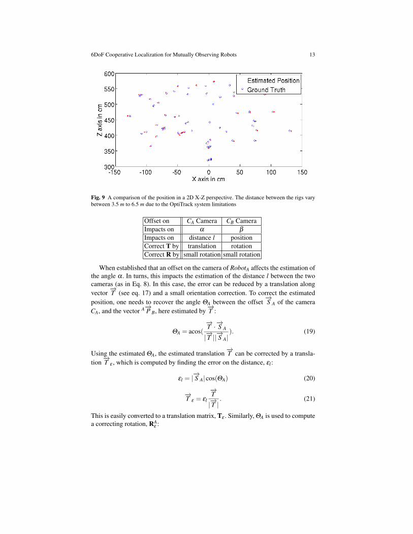
For the second data set, Fig. 8a shows its position error, with a mean error of1.9885 cm. Figure 8b shows its orientation error, with a mean error of 0.0205 rad, or1.175 degrees. Figure 9 shows the 2D perspective in the X-Z plane of the measuredand estimated positions of the moving camera setup.

Both test sets indicated that the orientation error is independent of the real orien-tation of the moving CameraB.


(a) (b)

Fig. 7 (a) Histogram representing the position error made by the bearing-only system for the cal-ibration dataset. The error mean is 2.4947 cm. (b) Histogram representing the orientation errormade by the bearing-only system for the calibration dataset. The error mean is 0.0370 rad.

(a) (b)

Fig. 8 (a) Histogram representing the position error made by the bearing-only system for the testdataset. The error mean is 1.9885 cm. (b) Histogram representing the orientation error made by thebearing-only system for the test dataset. The error mean is 0.0205 rad.

6 Non-Colinearity Analysis and Error Correction

In the previous sections, we presented an analytical solution to the 3D cooperativelocalization problem given that each robot’s camera Ci was collinear to its markersRi and Li. In order to measure the impact of non-colinearity on the localization error,we implemented a simulation in MATLAB where we added small offsets to theposition of the cameras. An offset applied to a camera is described by a translationof up to 35% of the distance d between a robot’s markers. This translation is orientedin a direction ranging from 0 to π rad in the plane defined by the vectors A−→P B and−→n A (equations 7 and 9, respectively). Thus, most realistic scenarios were coverred.In order to find a way to compute a correction to RobotB’s pose estimation, weinitially applied the offsets on only one camera. Table 6 above shows a summary ofthe impact of offset.


Fig. 9 A comparison of the position in a 2D X-Z perspective. The distance between the rigs varybetween 3.5 m to 6.5 m due to the OptiTrack system limitations

Offset on CA Camera CB CameraImpacts on α β

Impacts on distance l positionCorrect T by translation rotationCorrect R by small rotation small rotation

When established that an offset on the camera of RobotA affects the estimation ofthe angle α . In turns, this impacts the estimation of the distance l between the twocameras (as in Eq. 8). In this case, the error can be reduced by a translation alongvector

−→T (see eq. 17) and a small orientation correction. To correct the estimated

position, one needs to recover the angle ΘA between the offset−→S A of the camera

CA, and the vector A−→P B, here estimated by−→T :

ΘA = acos(−→T ·−→S A

|−→T ||−→S A|). (19)

Using the estimated ΘA, the estimated translation−→T can be corrected by a transla-

tion−→T ε , which is computed by finding the error on the distance, εl :

εl = |−→S A|cos(ΘA) (20)

−→T ε = εl

−→T

|−→T |. (21)

This is easily converted to a translation matrix, Tε . Similarly, ΘA is used to computea correcting rotation, RA

ε :


RAε = Rodrigues

(−−−→LARA,arcsin

(sin(ΘA)

|−→S A||−→T |+ εl

)). (22)

On the other hand, when the camera on RobotB has an offset the estimation ofthe angle β is affected. This impacts the estimation of the position, but conserves avalid distance l estimation. In this case, the error can be reduced by a rotation aboutthe RA-LA axis, again with a small orientation correction. To make these corrections,one needs to recover the angle ΘB between the offset

−→S B of the camera CB expressed

in FB, and the vector B−→P A, here estimated by −−→T , again expressed in FB:

ΘB = arccos

(R1−1R2

−1(−−→T )

|−→T |·−→S B

|−→S B|

). (23)

Using the estimated ΘB, the estimated translation−→T and the estimated orientation

R2R1 can be corrected by a rotation matrix RBε , which is computed by finding the

error on the orientation, εθ :

εθ = arcsin(sin(ΘB)|−→S B||−→T |+ εl

) (24)

RBε = Rodrigues(

−−−→LARA,εθ ). (25)

Since each camera offset has effects that are not related, we can sum the correc-tions independently, which leads to the revised equation 18:

AFB = RBε Tε TRB

ε RAε R2R1F ′B. (26)

We tested Eq. 26 in a simulation at a distance l = 11 m. We applied offsets of28 cm, or 35%d, in the direction of −→n A. This resulted in the greatest error duringthe estimation. After the correction, this simulation demonstrated that when the an-gle β is sharp, the position error could remain as high as 20 cm. This high errorcorresponds to the behavior that was observed in the 2D solution when the robotsare observing each other at a sharp angle. However, when both cameras were notcollinear and the RobotB was positionned at less than 45deg away from the centralpoint of RobotA’s camera, one could expect a position error of less than 3cm and anorientation error of about 0.006 rad.

We compared the position errors due to our correction in Eq. 18 to the positionerrors induced by mislocating the markers in the image, since the latter will af-fect the estimation of α and β . For this comparison, we chose an angular noise ofσϕ = 0.0003 for the computation of β , as well as an angular noise of σϕ ∗

√2 for

the measurement α . These values corresponded to an error of the estimation pointsin the image plane of approximately 0.3 pixel, close to what we observed in our sys-tem. The simulation results indicated that the average positional error for correctionwas generally less than 40% of the error due to the mislocation of the various land-marks. Consequently, our equation does not significantly affect the performance of


the system. However, this error correction is biased, and it should be kept in mind ifa filtering technique, such as EKF or UKF, is employed.

7 Conclusions and Future Work

In this paper we presented a novel analytical solution to the 3D Cooperative Local-ization problem using bearing only measurements between two robots. We derivedthe mathematical solution to the problem in three dimensions, which was verifiedwith extensive simulations and experiments with real hardware. During experimentswith a rig that moved freely in 6 DoF, our system demonstrated good positionestimation (average error around 2 cm over 250 samples), despite the use of off-the-shelf consumer cameras and markers. This makes our solution particularly wellsuited for deployment on fleets of inexpensive robots.

The biggest challenge with the current physical implementation is to establishmutual observations, without interfering with the normal operation of the vehicles.Since the method is completely compatible with any type of cameras, omnidirec-tional cameras can be employed to alleviate this problem.

We are currently planning to apply this methodology to under-actuated squareblimps that move at slow speeds [24], since the weight of the required hardware forour solution is very low. Applications to underwater vehicles [8] are also consid-ered, since they are generally deployed in unstructured, GPS-denied environments.Another direction of research will be to employ Iterated Sigma Point Kalman Fil-tering [25] in order to integrate additional sensors and improve the accuracy of thestate estimation.

References

1. Bahr, A., Leonard, J.J., Fallon, M.F.: Cooperative localization for autonomous underwatervehicles. The Int. Journal of Robotics Research 28(6), 714–728 (2009)

2. Burgard, W., Moors, M., Fox, D., Simmons, R., Thrun, S.: Collaborative multi-robot explo-ration. In: Proc. of IEEE Int. Conf. on Robotics and Automation, vol. 1, pp. 476–481 (2000)

3. Cognetti, M., Stegagno, P., Franchi, A., Oriolo, G., Bulthoff, H.H.: 3-d mutual localizationwith anonymous bearing measurements. In: Proc. IEEE Int. Conf. on Robotics and Automa-tion, pp. 791–798 (2012)

4. Cristofaro, A., Martinelli, A.: 3D cooperative localization and mapping: Observability analy-sis. In: American Control Conf. (ACC), 2011, pp. 1630–1635. IEEE (2011)

5. Davison, A.J., Kita, N.: Active visual localisation for cooperating inspection robots. In: Proc.of IEEE/RSJ Int. Conf. on Intel. Robots and Systems, vol. 3, pp. 1709–1715 (2000)

6. Dhiman, V., Ryde, J., Corso, J.J.: Mutual localization: Two camera relative 6-dof pose estima-tion from reciprocal fiducial observation. arXiv preprint arXiv:1301.3758 (2013)

7. Dieudonne, Y., Labbani-Igbida, O., Petit, F.: Deterministic robot-network localization is hard.IEEE Transactions on Robotics 26(2), 331–339 (2010)

8. Dudek, G., Jenkin, M., Prahacs, C., Hogue, A., Sattar, J., Giguere, P., German, A., Liu, H.,Saunderson, S., Ripsman, A., Simhon, S., L-A Torres, L.A., Milios, E., Zhang, P., Rekleitis,I.: A visually guided swimming robot. In: IEEE/RSJ Int. Conf. on Intel. Robots and Systems,pp. 3604–3609 (2005)


9. Fischler, M.A., Bolles, R.C.: Random sample consensus: a paradigm for model fitting withapplications to image analysis and automated cartography. Communications of the ACM24(6), 381–395 (1981)

10. Franchi, A., Stegagno, P., Oriolo, G.: Probabilistic mutual localization in multi-agent sys-tems from anonymous position measures. In: 49th IEEE Conf. on Decision and Control, p.65346540. Atlanta, GA (2010)

11. Gage, D.W.: Minimum-resource distributed navigation and mapping. Tech. rep., DTIC (2000)12. Giguere, P., Rekleitis, I., Latulippe, M.: I see you, you see me: Cooperative Localization

through Bearing-Only Mutually Observing Robots. In: IEEE/RSJ Int. Conf. on Intel. Robotsand Systems,, pp. 863–869. Portugal (2012)

13. Huang, G., Trawny, N., Mourikis, A., Roumeliotis, S.: Observability-based consistent ekf es-timators for multi-robot cooperative localization. Autonomous Robots 30(1), 99–122 (2011)

14. Kato, K., Ishiguro, H., Barth, M.: Identifying and localizing robots in a multi-robot systemenvironment. In: Proc. of IEEE/RSJ Int. Conf. on Intel. Robots and Systems, vol. 2, pp. 966–971 (1999)

15. Kennedy, R., Daniilidis, K., Naroditsky, O., Taylor, C.: Identifying maximal rigid componentsin bearing-based localization. In: IEEE/RSJ Int. Conf. on Intel. Robots and Systems, pp.194–201 (2012). DOI 10.1109/IROS.2012.6386132

16. Kukelova, Z., Bujnak, M., Pajdla, T.: Closed-form solutions to minimal absolute pose prob-lems with known vertical direction. Computer vision–ACCV 2010 pp. 216–229 (2011)

17. Kurazume, R., Hirose, S.: An experimental study of a cooperative positioning system. Au-tonomous Robots 8, 43–52 (2000)

18. Kurazume, R., Nagata, S., Hirose, S.: Cooperative positioning with multiple robots. In: IEEEInt. Conf. on Robotics and Automation, vol. 2, pp. 1250–1257 (1994)

19. Naroditsky, O., Daniilidis, K.: Optimizing polynomial solvers for minimal geometry prob-lems. In: IEEE Int. Conf. on Computer Vision, pp. 975–982 (2011)

20. Rekleitis, I., Dudek, G., Milios, E.: Experiments in free-space triangulation using cooperativelocalization. In: IEEE/RSJ/GI Int. Conf. on Intel. Robots and Systems, pp. 1777–1782 (2003)

21. Rekleitis, I., Dudek, G., Milios, E.: Probabilistic cooperative localization and mapping in prac-tice. In: IEEE Int. Conf. on Robotics and Automation, pp. 1907–1912 (2003)

22. Rekleitis, I.M., Dudek, G., Milios, E.E.: On multiagent exploration. In: Proc. of Vision Inter-face 1998, pp. 455–461. Vancouver, Canada (1998)

23. Roumeliotis, S., Bekey, G.: Collective localization: A distributed kalman filter approach tolocalization of groups of mobile robots. In: IEEE Int. Conf. on Robotics and Automation, pp.2958–2965 (2000)

24. Sharf, I., Persson, M.S., St-Onge, D., Reeves, N.: Development of aerobots for satellite emu-lation, architecture and art. In: Proc. the 13th Int. Symp. on Experimental Robotics (2012)

25. Sibley, G., Sukhatme, G., Matthies, L.: The iterated sigma point kalman filter with applicationsto long range stereo. In: Proc. of Robotics: Science and Systems, pp. 263–270 (2006)

26. Spletzer, J.R., Taylor, C.J.: A bounded uncertainty approach to multi-robot localization. In:Proc. of IEEE/RSJ Int. Conf. on Intel. Robots and Systems, vol. 2, pp. 1258–1265 (2003)

27. Weber, B., Zeller, P., Kuhnlenz, K.: Multi-camera based real-time configuration estimationof continuum robots. In: IEEE/RSJ Int. Conf. on Intel. Robots and Systems, pp. 3350–3355(2012)

28. Zhou, X., Roumeliotis, S.: Determining the robot-to-robot 3D relative pose using combina-tions of range and bearing measurements: 14 minimal problems and analytical solutions to 3of them. In: Proc. IEEE/RSJ Int. Conf. on Intel. Robots and Systems, pp. 2983–2990 (2010)

29. Zhou, X., Roumeliotis, S.: Determining the robot-to-robot 3D relative pose using combina-tions of range and bearing measurements (part ii),. In: Proc. IEEE Int. Conf. on Robotics andAutomation, pp. 4736–4743. Shanghai, China (2011)

30. Zhou, X., Roumeliotis, S.: Determining 3D relative transformations for any combination ofrange and bearing measurements. IEEE Transactions on Robotics (2012)

Documents

6DoF Cooperative Localization for Mutually Observing Robotspgiguere/papers/isrr2013.pdf · 6DoF Cooperative Localization for Mutually Observing Robots 3 The accuracy of vision-based