Assessing the stability of long-horizon SSA forecasting

with application to the analysis of Earth temperatures

Abstract

We start with formalizing the problem of assessing the stability of long-horizon forecast-

ing of a given family of forecasting techniques. Next, we argue that in some applications

the so-called singular-spectrum analysis (SSA) could be a suitable family of techniques to

consider. We then apply the methodology to two simulated time series and also to the

Earth temperature records. We demonstrate that the SSA forecasts of the temperatures

appear to be more stable at present than three-four years ago.

Keywords: Singular spectrum analysis, retrospective forecasts, long-horizon forecast-

ing, stability of forecasts, SSA vector forecasting

1 Assessing the stability of forecasts

Assume that we have a time series x1, . . . , xT and our aim is to make an h-step forecast for

this series, where the horizon h is relatively large (for example, h = 100). We assume that

the structure of the series x1, x2, . . . is complex and may not be very stable; an implication

of this is the inadequacy of the assumption of the stationarity of the series. We, however,

assume that the changes in the structure do not occur often and these changes are relatively

small. In particular, we assume that these changes are not going to dramatically alter the

behaviour of the series during the forecasting period.

We also assume that we have a family of forecasting techniques and wish to assess

the reliability of the corresponding h-step forecasts. More precisely, we want to make an

opinion about how much can we trust our h-step forecast xT+h.

Evaluation of the quality of forecasts. To evaluate the accuracy and reliability

of the forecasts, one can use a suitable combination of the following three approaches: (a)

construction of confidence intervals; (b) assessment of retrospective forecasts; (c) checking

stability of forecasts.

The approach (a) is based on the use of parametric models of the series and/or on

the bootstrap techniques. These parametric models are either assumed (for example,

1

ARIMA) or built in the process of analysis (SSA). In the long-horizon forecasting the use

of confidence bounds is very limited and often even useless. For example, in the ARIMA-

type models the confidence intervals become very wide for large h. In SSA and similar

techniques the confidence intervals do not increase fast but they depend on the accuracy

of the constructed model and on the fact that this model is not going to break during the

forecasting period.

Retrospective forecasts (the approach (b) above) are performed by truncating the series

and forecasting values at the points temporarily removed. These forecasts can then be

compared with the observed values of the time series for making an assessment of the

quality of the forecasts. The use of the retrospective forecasts is important, especially

when h is small. In the situation we consider, its usefulness is very limited in view of the

magnitude of h and the instability of the structure of the series.

Despite we do not dismiss the approaches (a) and (b), in the present paper we only

concentrate on the approach (c); that is, on the assessing the stability of forecasts.

Creation of the samples of the forecast values. Assume that we have a family

of forecasting techniques which is parameterized by a parameter θ ∈Θ⊂Rm. Here Θ is

an m-dimensional set of admissible values; some components of θ ∈ Θ may take values on

the ordinal or even nominal scale (which would correspond to switches between groups of

methods). Any θ∈Θ defines a particular forecasting technique from the chosen family of

techniques.

We may be interested in the forecast to horizons which are approximately h rather

than exactly h; that is, to the domain of horizons g ∈ [h1, h2] with 0 < h1≤ h≤ h2 <∞.

Choosing an interval of horizons rather than a single horizon makes sense, for example,

if we are not interested in the quality of extracted seasonality components but are much

more interested in the general tendency and the related variability of the forecasts. On the

other hand, if we expect strong trend and/or strong seasonality in the future behaviour of

the series then the choice h1∼= h2 seems to be more reasonable.

For each time moment t≤ T , any g > 0 and any θ ∈ Θ we can build a g-step ahead

forecast x̂t+g(θ) based on the information x1, . . . , xt. Hence for any t≤T we may compute

the following set of forecasting results:

Ft = {x̂T+g(θ) : g ∈ [h1, h2], θ ∈ Θ}. (1)

2

Here the subscript t designates that the forecasts are based on the use of the subseries

x1, . . . , xt.

If the main interest of the study is the quality of the h-step ahead forecasting procedures

(for example, when we compare two families of forecasting techniques), then the following

set of forecasting results may also be of interest: {x̂t+g(θ) : g ∈ [h1, h2], θ ∈ Θ}.If Θ is a finite set then the sets Ft are finite, otherwise (if some components of θ ∈ Θ

take values at an infinite set) we need to take a sufficiently representative sample of values

θi ∈ Θ and approximate the sets (1) by finite sets which we shall call samples (of the

values of the forecasts). In what follows we assume that the set Θ = {θ1 . . . , θm} is finite.

The number of elements in the samples Ft is M =m(h2−h1+1).

Summarizing, our forecasting procedure allows us to get T − T0 + 1 samples Ft =

{f (t)1 , . . . , f

(t)M } computed according to (1) at all t = T0, . . . , T where T0 is the first time

moment we applied the forecasting procedures.

Comparison of the samples Ft. We now need to compare the samples Ft (t =

T0, . . . , T ) to evaluate the stability of the corresponding forecasts and decide whether at

t = T we have reached an acceptable level of stability.

The mean values of the samples Ft are f̄t = (f (t)1 + . . . + f

(t)M )/M . Ideally, the sequence

of these mean values should approach the true value of the expectation of xT+h under the

following assumptions: h1 = h2, m → ∞, the model of the time series is signal + noise,

the signal have been fully extracted and extrapolated by the forecasting techniques, and

the structure of the series has stayed unchanged for a period of time significantly longer

than h. These assumptions are unrealistic and are impossible to check (unless we are doing

simulation experiments). Moreover, the fact whether the values f̄t are approaching ExT+h

or not is not important if we consider the stability of the forecasts.

As measures of stability, we must consider the behaviour of some characteristics of

variability of the samples Ft. The simplest and perhaps most natural among these char-

acteristics is the (empirical) standard deviation of Ft:

st =

√√√√ 1M − 1

M∑

i=1

(f (t)i − f̄t)2 . (2)

We may say, for example, that the series x1, . . . , xT leads to a more stable forecast than

the subseries x1, . . . , xt (with t < T ) if the standard deviation sT is significantly smaller

3

than the standard deviation st.

One of the reasons for the importance of st is the observation that under some natural

assumptions the lengths of the asymptotic confidence intervals for the mean values of

the forecasts are proportional to the values of st. Note that we can also use some robust

estimators of the standard deviation of the distribution which the sample Ft corresponds to.

In addition to the standard deviation st, we would recommend to consider another

important characteristic of sample variability, the range of the sample Ft:

Rt = maxi=1,...,M

f(t)i − min

i=1,...,Mf

(t)i .

One may decide to prefer the range Rt over the standard deviation st if the main emphasis

in the study is on the worst-case (guaranteed) performance of the forecasts rather than on

their behaviour in most cases.

2 SSA and other families of forecasting techniques

Combined error of any forecast is due to the random error (associated with noise) and the

bias (associated with the chosen forecasting technique).

In this study, we treat the time series purely as a set of numbers. Usually, however,

there is some randomness in the data which gives rise to some random error in the forecast,

even we try to filter the noise out (as SSA does). There is also bias in the forecast associated

with the chosen model and the group of forecasting techniques: precise prediction of the

future is not generally possible.

Thus, there is very little hope of building a very accurate forecast for the medium/long

horizons. We however may hope to find a rich family of forecasting techniques whose

forecasts are becoming more and more stable as the amount of information about the

series increases.

ARIMA and similar models The majority of the classical forecasting techniques

(with ARMA as the main example) use the assumption of stationarity of the series; to

achieve the stationarity it is customary to make the differencing of the series (leading to

ARIMA-type models) or extract a non-stationary trend using regression. In addition to

the assumption of stationarity, which we are not prepared to assume, there are at least

4

two more obstacles preventing the use of ARIMA-type techniques in our studies: (a) the

confidence intervals for the forecasted values at long horizons are typically very wide, and

(b) the choice of parameters in these techniques is usually automatic and it is not obvious

how to create a rich and representative family of these techniques.

The use of change-point detection techniques Since we assume that certain

changes in the structure of the series x1, x2, . . . may occur, the following strategy for

analyzing these series seems to be very reasonable: (a) use a suitable change-point detection

technique, (b) if a change in the structure of the series is detected then disregard the initial

part of the series, and (c) apply one of standard techniques for analyzing and forecasting

the remaining part of the series.

However, we are not going to use this approach. One of the reasons for this is that the

use of change-point detection techniques would contradict to the main aim of the study

which is the verification of the fact that all of the chosen past of the series is homogeneous

enough to provide stable forecasts based on all previous information; a removal of a part

of the series would confront this.

Singular spectrum analysis (SSA) While using SSA neither a parametric model

nor stationarity-type conditions have to be assumed for the time series; this makes SSA a

model-free technique. SSA is robust to small changes in the structure of the series which

makes SSA to be an ideal tool in our study. We shall be using the basic version described in

the introduction to this volume [2]; note that we shall also be using the notation introduced

in [2].

SSA forecasting There are several ways of constructing forecasts based on the SSA

decomposition of the series described above, see Chapter 2 in [3]. The most obvious way

is to use the linear recurrent formula which the series reconstructed from X̃ satisfies. We

however prefer to use the so-called ’SSA vector forecast’ ([3], Sect. 2.3.1). The main

idea of the SSA vector forecasting algorithm is as follows. Selection of r eigenvectors of

XXT leads to the creation of the subspace Sr. SVD properties give us a hope that the

L-dimensional vectors {X1, . . . , XK} lie close to this subspace. The forecasting algorithm

then sequentially constructs the vectors {XK+1, XK+2, . . .} so that they stay as close as

5

possible to the chosen subspace Sr.

Choice of SSA parameters In the examples below, the length of the series is T ∼= 300

and the forecasting horizon is h ∼= 100. If the structure of the series is assumed stable

then large values of L, of the order L ∼= 100, should be preferred to small values, of the

order L ∼= 10. We, however, assume that the structure of the series is not rigid (despite

in Example 2 below the structure is stable). In this case, large values of L would not

give SSA enough flexibility to react to the changes (which we assume rare and slow). On

the other hand, for small values of L, SSA may be too sensitive to the noise and small

variations in the trend. It is therefore natural to select values of L somewhere in-between.

Our choice is 20 ≤ L ≤ 50 which we believe is a rather broad range.

The second SSA parameter to choose is r, the dimension of the subspace Sr. The choice

of r should depend on what do we intend to forecast. For example, if we observe some

seasonal variations in the data and we want to forecast these variations, then we have to

choose r large enough to capture these variations (see Example 2 below). On the other

hand, if the analysis shows that these variations are insignificant and the only tendency of

interest is the general trend, then the value of r should be small (see Example 1). There

are several procedures (see e.g. [3]) for choosing the most suitable value of r (roughly

speaking, r should be the smallest among those values of r for which the residuals after

signal extraction pass the chosen statistical tests for being a noise). These procedures,

however, are often not very reliable and are not well suited for the long-term forecasting

which is the purpose of our study.

We realize that whatever the rule of selection of r, some values of r are too small,

which leads to us missing parts of the signal, but other values of r are too large, which

means that we include a significant part of the noise into the ‘reconstructed signal’. This,

however, goes in line with the purpose of our study which is checking the stability of the

forecasts with respect to both the signal and noise behavior.

3 Simulated examples

In the following two examples we try to emulate some features of the main example con-

sidered in Section 4. In both examples, the length of the series is T = 300 and the first

6

time moment where the forecasts start is N − n + 1 = 230. All forecasts are made by

the SSA vector forecasting algorithm for h steps, where either h = 100 or h ' 100. The

window length L in the SSA algorithm takes all the values in the interval L ∈ [20, 50].

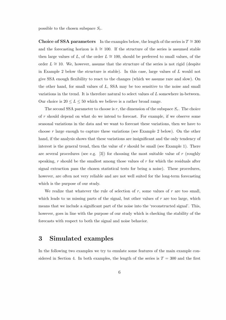
Simulated example 1 Let the time series be

xt =

−5(1− t/200)2 + εt for t = 1, . . . , 200

εt for t = 201, . . . , 300

where εt are independent Gaussian random variables with mean 0 and variance 1. Note

that there is a gradual change of structure of this series just before the time t = 200.

Figure 1: Example 1. The time series (gray), the SSA approximation and the forecast for L = 50

and r = 3 (black).

We only consider a single realization of this series shown in Figure 1. This figure also

shows a typical SSA approximation (which we obtain for L = 50 and r = 3) and the

corresponding forecast.

7

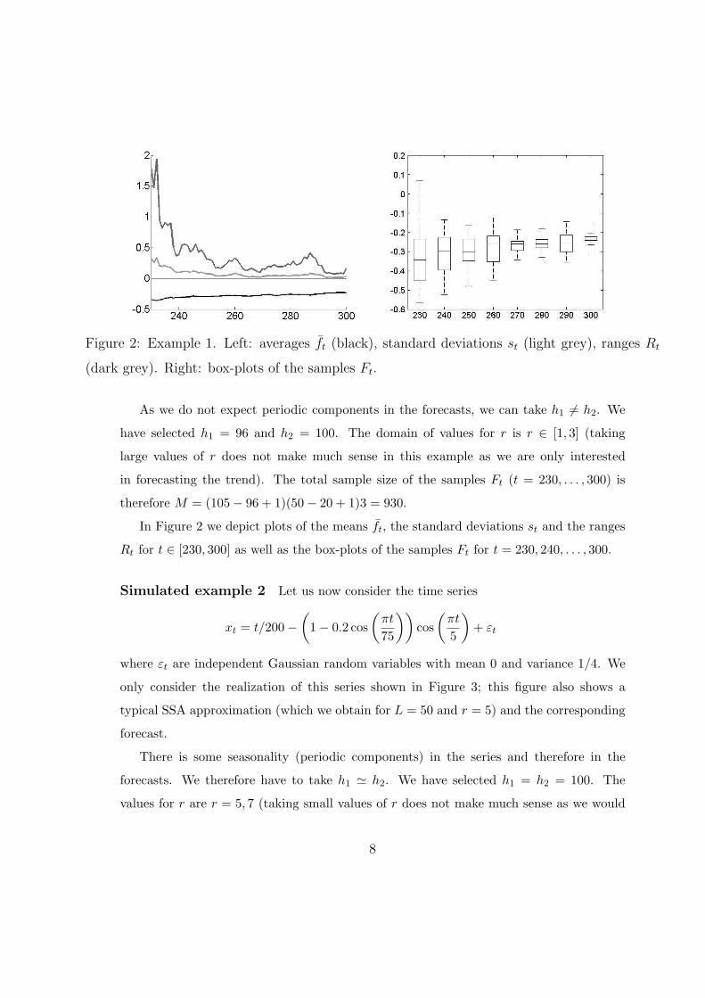
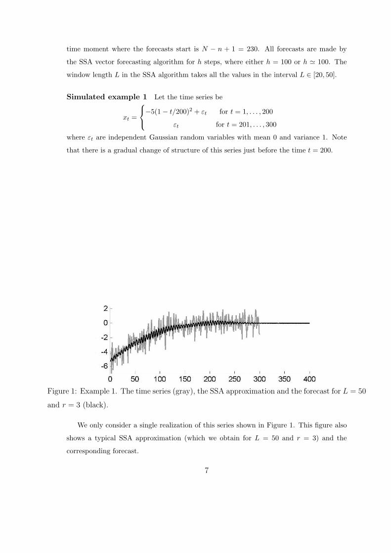
Figure 2: Example 1. Left: averages f̄t (black), standard deviations st (light grey), ranges Rt

(dark grey). Right: box-plots of the samples Ft.

As we do not expect periodic components in the forecasts, we can take h1 6= h2. We

have selected h1 = 96 and h2 = 100. The domain of values for r is r ∈ [1, 3] (taking

large values of r does not make much sense in this example as we are only interested

in forecasting the trend). The total sample size of the samples Ft (t = 230, . . . , 300) is

therefore M = (105− 96 + 1)(50− 20 + 1)3 = 930.

In Figure 2 we depict plots of the means f̄t, the standard deviations st and the ranges

Rt for t ∈ [230, 300] as well as the box-plots of the samples Ft for t = 230, 240, . . . , 300.

Simulated example 2 Let us now consider the time series

xt = t/200−(

1− 0.2 cos(

πt

75

))cos

(πt

5

)+ εt

where εt are independent Gaussian random variables with mean 0 and variance 1/4. We

only consider the realization of this series shown in Figure 3; this figure also shows a

typical SSA approximation (which we obtain for L = 50 and r = 5) and the corresponding

forecast.

There is some seasonality (periodic components) in the series and therefore in the

forecasts. We therefore have to take h1 ' h2. We have selected h1 = h2 = 100. The

values for r are r = 5, 7 (taking small values of r does not make much sense as we would

8

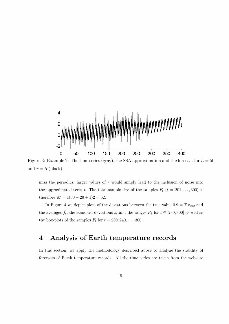
Figure 3: Example 2. The time series (gray), the SSA approximation and the forecast for L = 50

and r = 5 (black).

miss the periodics; larger values of r would simply lead to the inclusion of noise into

the approximated series). The total sample size of the samples Ft (t = 201, . . . , 300) is

therefore M = 1(50− 20 + 1)2 = 62.

In Figure 4 we depict plots of the deviations between the true value 0.9 = Ex400 and

the averages f̄t, the standard deviations st and the ranges Rt for t ∈ [230, 300] as well as

the box-plots of the samples Ft for t = 230, 240, . . . , 300.

4 Analysis of Earth temperature records

In this section, we apply the methodology described above to analyze the stability of

forecasts of Earth temperature records. All the time series are taken from the web-site

9

Figure 4: Example 2. Left: shifted averages 0.9− f̄t (black), standard deviations st (light grey),

ranges Rt (dark grey). Right: the box-plots of the samples Ft.

http://vortex.nsstc.uah.edu/ (National Space Science and Technology Center, USA,

NASA). These series represent the temperature on Earth during the last 30 years and are

widely discussed in literature, see for example, [4].

The series are the so-called temperature anomalies rather than the absolute tempera-

tures (temperature anomalies are computed relative to the base period 1951-1980). Work-

ing with anomalies rather than with absolute temperature records is customary in clima-

tology, see for example the publications and web-sites of the Goddard Institute for Space

Studies. The first data point in each series is December 1978, the last is December 2009

so that altogether we have T = 373 data points. The first time moment we start the fore-

casts is January 2005 implying T0 = 314. We forecast the series until 2018 (longer-term

forecasts are very similar) by setting h1 = 97, h2 = 99.

As in examples above we select the domain L ∈ [20, 50] for the SSA window length L.

Similar to Example 2, we choose the first r ∈ [5, 7] eigenvectors. Despite a better forecast

(with better stability) can be obtained if we optimize the domains of parameters L and

r for each individual series, we have fixed the domains to show the robustness of results.

Furthermore, the results of our study are very stable with respect to these domains.

We have selected the global temperature on Earth, Northern Hemisphere temperature

and North Pole temperature. These three series of temperatures are discussed most often.

10

We have done similar analysis for some other series; the results are presented at the web-

site [1]. This web-site also contains more results for the series considered here.

For each of the three chosen temperature series we plot the following.

(i) Figures 5, 8 and 11: the series itself, the SSA approximation and SSA forecast for

L = 50 and r = 7 computed at the last point t = T (December 2009).

(ii) Figures 6, 9 and 12 (left): the series −f̄t, standard deviations st (light grey), ranges

Rt (dark grey) for t = 314, . . . , 373 (the averages f̄t are always plotted with the minus

sign for the purpose of clarity of display).

(iii) Figures 6, 9 and 12 (right): box-plots of the samples Ft for t = 325, 337, 349, 361, 373.

(iv) Figures 7, 10 and 13: forecasts for the temperature at January 2018 using the series

x1, . . . , xt for L = 20, 30, 40, 50, r = 5, 7 and all t = 314, . . . , 373.

Note that the markers on the x-axis in all plots correspond to Januaries. To compare

the forecasted values of the temperatures with the recent values, note the average values

of these temperatures during the last ten years 2000–2009: 0.222 for Earth; 0.312 for

Northern Hemisphere; 0.859 for North Pole.

We can observe that the standard deviation st is smaller during last 2 years that

during 2005 year. We can also see that forecasts at 2018 are very close to the averaged

temperatures during the last ten years 2000–2009 meanwhile forecasts at 2018 based on

series truncated until 2005–2006 is significantly larger than these averaged temperatures.

References

[1] Web-site with supplement materials http://earth-temperature.com/stability/

[2] Zhigljavsky, A. (2010). Singular spectrum analysis: the state-of-the-art. Introduction

to the present issue

[3] Golyandina, N., Nekrutkin, V. and Zhigljavsky, A. (2001). Analysis of Time Series

Structure: SSA and related techniques. Chapman & Hall/CRC.

[4] Plimer I. (2009). Heaven and Earth: Global Warming - The Missing Science. Quartet

books, London.

11

[5] Vautard, R., Yiou, P. and Ghil, M. (1992). Singular-spectrum analysis: A toolkit for

short, noisy chaotic signal. Physica D 58, 95–126.

12

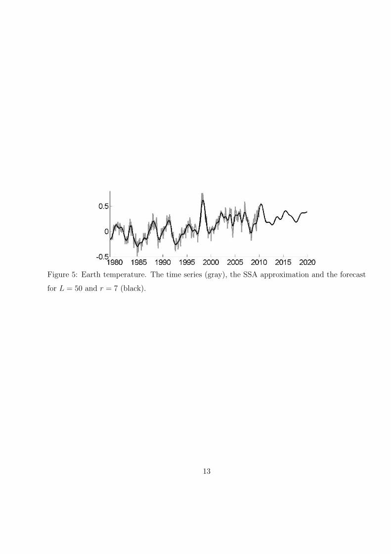
Figure 5: Earth temperature. The time series (gray), the SSA approximation and the forecast

for L = 50 and r = 7 (black).

13

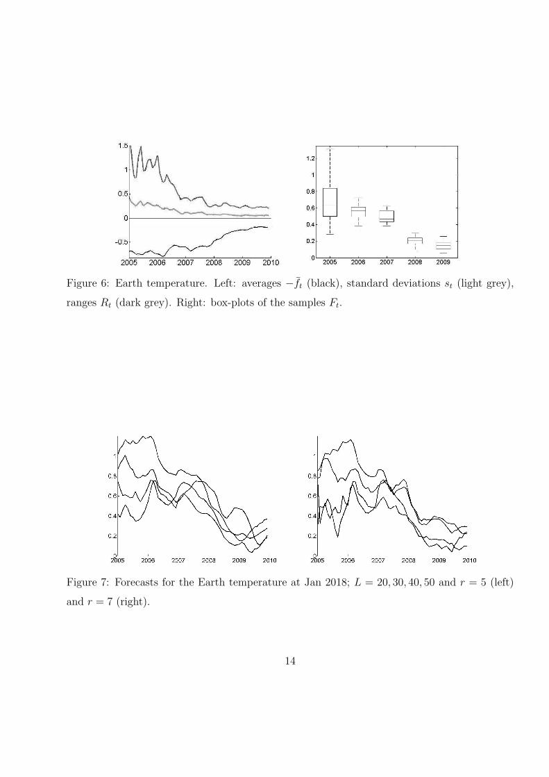
Figure 6: Earth temperature. Left: averages −f̄t (black), standard deviations st (light grey),

ranges Rt (dark grey). Right: box-plots of the samples Ft.

Figure 7: Forecasts for the Earth temperature at Jan 2018; L = 20, 30, 40, 50 and r = 5 (left)

and r = 7 (right).

14

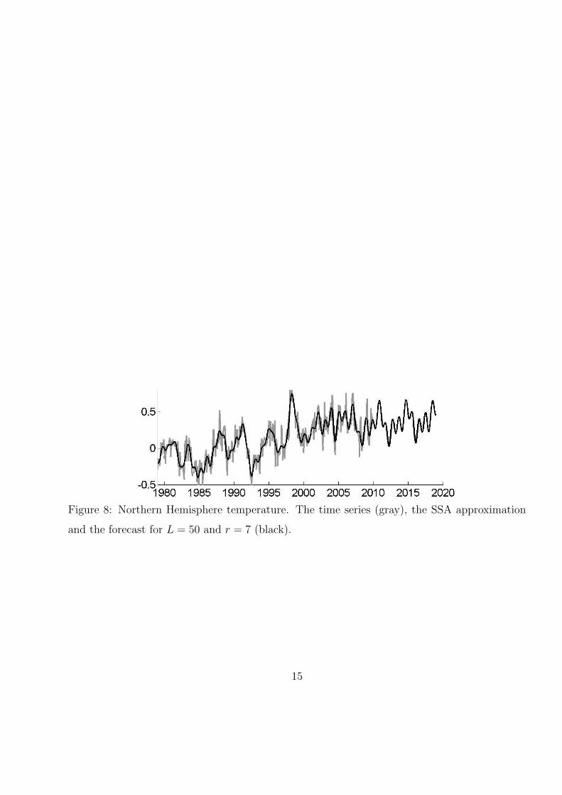
Figure 8: Northern Hemisphere temperature. The time series (gray), the SSA approximation

and the forecast for L = 50 and r = 7 (black).

15

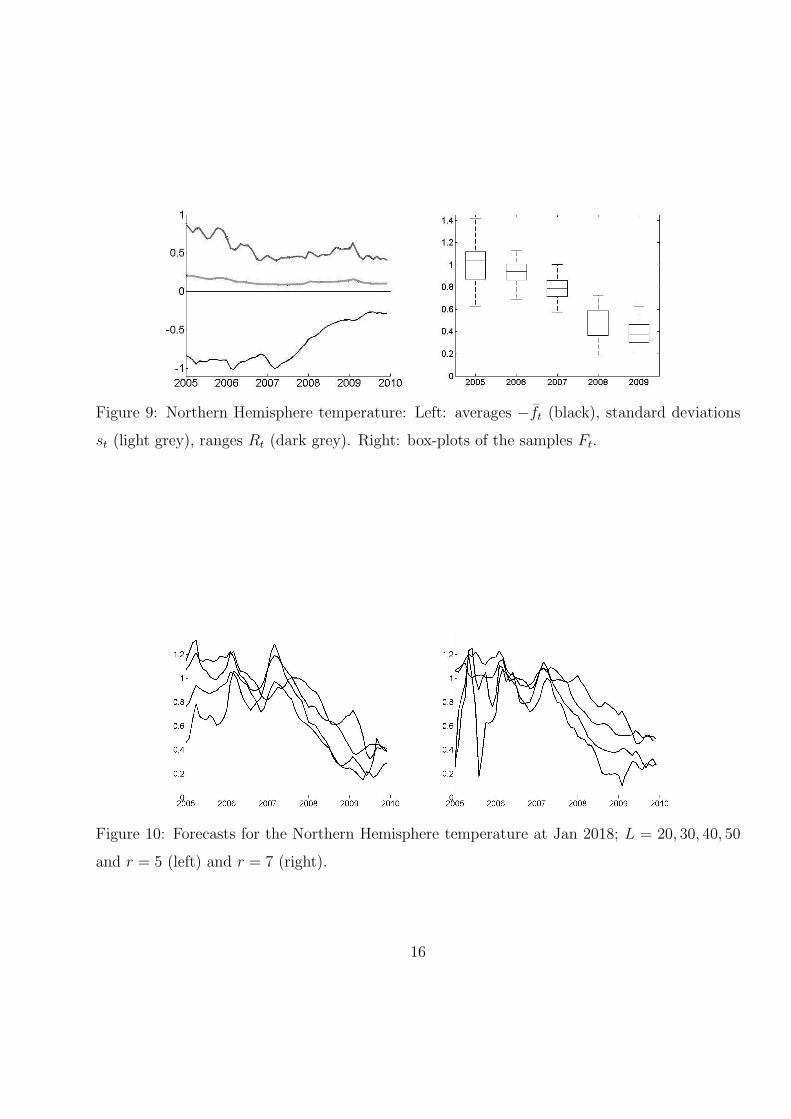
Figure 9: Northern Hemisphere temperature: Left: averages −f̄t (black), standard deviations

st (light grey), ranges Rt (dark grey). Right: box-plots of the samples Ft.

Figure 10: Forecasts for the Northern Hemisphere temperature at Jan 2018; L = 20, 30, 40, 50

and r = 5 (left) and r = 7 (right).

16

Figure 11: North Pole temperature. The time series (gray), the SSA approximation and the

forecast for L = 50 and r = 7 (black).

17

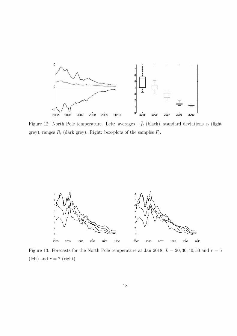
Figure 12: North Pole temperature. Left: averages −f̄t (black), standard deviations st (light

grey), ranges Rt (dark grey). Right: box-plots of the samples Ft.

Figure 13: Forecasts for the North Pole temperature at Jan 2018; L = 20, 30, 40, 50 and r = 5

(left) and r = 7 (right).

18