Embed Size (px)
Citation preview

1 © Alexis Kwasinski, 2011
•DC micro-grids comprise cascade distributed power architectures – converters act as interfaces
•Point-of-load converters present constant-power-load (CPL) characteristics
•CPLs introduce a destabilizing effect
lim
lim
0 if ( )( ) if ( )
( )L
v t VPi t v t V
v t
2B L
B B
dv Pz
di i
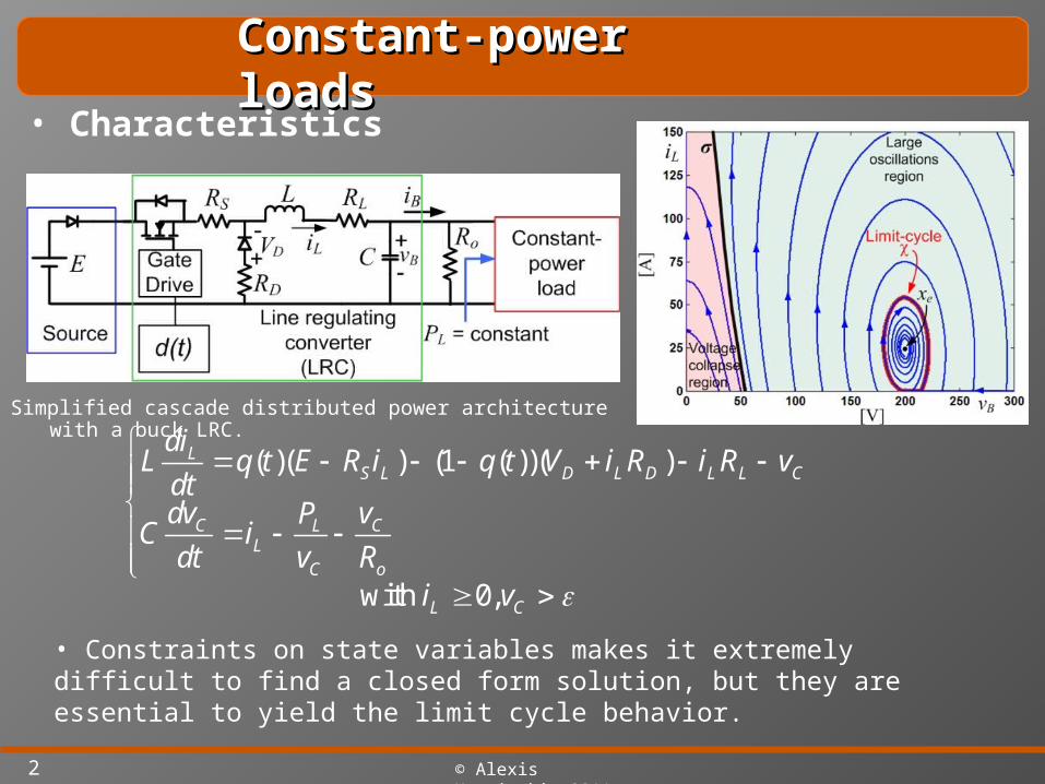
Constant-power loadsConstant-power loads
• Characteristics
2 © Alexis Kwasinski, 2011
Simplified cascade distributed power architecture with a buck LRC.
• Characteristics
Constant-power loadsConstant-power loads
( )( ) (1 ( ))( )
with 0,
LS L D L D L L C
C CLL
C o
L C
diL q t E R i q t V i R i R v
dtdv vP
C idt v R
i v
• Constraints on state variables makes it extremely difficult to find a closed form solution, but they are essential to yield the limit cycle behavior.

3 © Alexis Kwasinski, 2011
• The steady state fast average modelyields some insights:
• Lack of resistive coefficient in first-order term
• Unwanted dynamics introduced by the second-order term can not be damped.
• Necessary condition for limit cycle behavior:
• Note: x1 = iL and x2 = vC
22 2
22 22
22 1
2
with and 0
L
L
d x LP dxLC x DE
dtdt xdx P
x x Cdt x
• Characteristics
Constant-power loadsConstant-power loads
2
( ) 1C L LL
C C
d t E v P Pi
L C v v
4 © Alexis Kwasinski, 2011
Constant-power loadsConstant-power loads
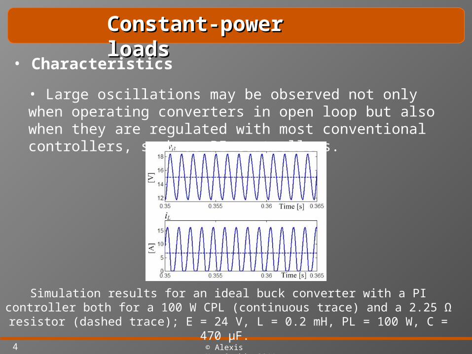
• Large oscillations may be observed not only when operating converters in open loop but also when they are regulated with most conventional controllers, such as PI controllers.
Simulation results for an ideal buck converter with a PI controller both for a 100 W CPL (continuous trace) and a 2.25 Ω resistor (dashed trace); E = 24 V, L = 0.2 mH,
PL = 100 W, C = 470 μF.
• Characteristics
5 © Alexis Kwasinski, 2011
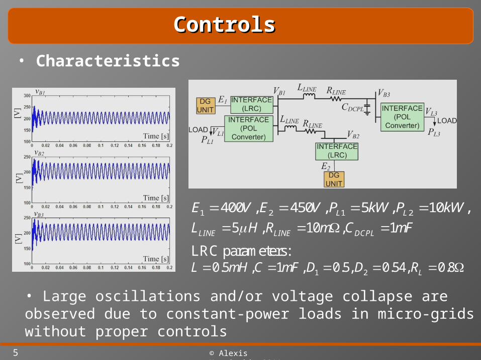
1 2 1 2400 , 450 , 5 , 10 ,L LE V E V P kW P kW
LRC parameters:
5 , 10 , 1LINE LINE DCPLL H R m C mF
1 20.5 , 1 , 0.5, 0.54, 0.8LL mH C mF D D R
• Large oscillations and/or voltage collapse are observed due to constant-power loads in micro-grids without proper controls
ControlsControls
• Characteristics
6 © Alexis Kwasinski, 2011
A system
with
f is locally Lipschitz
and
f(0,0) = h(0,0) = 0
is passive if there exists a continuously differentiable positive definite function H(x) (called the storage function) such that
0( , ), (0) , : R R R:
( , ), : R R R
n n m n
n m p
x f x u x x R f
y h x u h
( ) ( , ) ( , ) R RT n mdHH x f x u u y x u
dx
• Linear controllers – Passivity based analysis
StabilizationStabilization
• Initial notions
7 © Alexis Kwasinski, 2011
• Σ is output strictly passive if:
• A state-space system is zero-state observable from the output y=h(x), if for all initial conditions we have
• Consider the system Σ. The origin of f(x,0) is asymptotically stable (A.S.) if the system is
- strictly passive, or
- output strictly passive and zero-state observable.
- If H(x) is radially unbounded the origin of f(x,0) is globally asymptotically stable (A.S.)
- In some problems H(x) can be associated with the Lyapunov function.
2( ) ( , ) y ( , ) R R , and 0T n m
o o
dHH x f x u u y x u
dx
( ), R nx f x x (0) R nx ( ) 0 ( ) 0y t x t
• Linear controllers – Passivity based analysis
StabilizationStabilization
• Initial notions

8 © Alexis Kwasinski, 2011
[ ( )]x x x d M J R E
22
0 0( )
0 LP
x
x
R0
0
L
C
M0 1
1 0
J
0
E
E 1
2
xx
x
• Linear controllers – Passivity based analysis
StabilizationStabilization
• Consider a buck converter with ideal components and in continuous conduction mode. In an average sense and steady state it can be represented by
where
[ ( )] [ ( )] ex x x d x x M J R E J R
ex x x
LPL DE
eo
Ix
V DE
Equilibrium point:
(Coordinate change)
(1)
[ ( )]x x x d M J R E

9 © Alexis Kwasinski, 2011
22 2
1 L
i
P
R x
•Define the positive definite damping injection matrix Ri as
1
22 2
0
10
i
i L
i
R
P
R x
R
Ri is positive definite if . Then,
• Linear controllers – Passivity based analysis
StabilizationStabilization
: [ ] 0tx x M J R
[ ] [ ( )] ( )t e ix x d x x x x M J R E J R R
From (1), add on both sides:
0E
1
2
0
10
i
t i
i
R
R
R R R
(Equivalent free evolving system)
( )i x xR

10 © Alexis Kwasinski, 2011
1( )
2Tx x xH M
• Consider the storage function
• Linear controllers – Passivity based analysis
StabilizationStabilization
• is a free-evolving output strictly passive and zero-state observable system. Therefore, is an asymptotically stable equilibrium point of the closed-loop system.
( ) [ ] 0T T Tt tx x x x x x x H M J R R
Its time derivative is:
y x
2 1
2
1( ) = , where max ,T
t o o ii
x y y y RR
H R
0x
if

11 © Alexis Kwasinski, 2011
[ ( )] ( ) 0e id x x x x E E J R R
1 1
2
2 2 2
0
0
o i
oLL
i i
dE V R x
VP xI
x R R
• Since
then,
• Linear controllers – Passivity based analysis
StabilizationStabilization
Hence,
1 22
LPx Cx
x
1 1
1( )o i Ld V R x I
E
2( )Oe V x
and since and
1 11 2 2
2 2
1 i ii o o
i i
R Rd R Cx x V V
E R R
Thus,
This is a PD controller
2
2 2 2
o LL
i i
V P xI
R x R

12 © Alexis Kwasinski, 2011
• Remarks for the buck converter:• xe is not A.S. because the duty cycle must be between 0 and 1• Trajectories to the left of γ need to have d >1 to maintain stability• Using this property as the basis for the analysis it can be obtained that a necessary but not sufficient condition for stability is
• Line and load regulation can be achieved by adding an integral term but stability is not ensured
• Linear controllers – Passivity based analysis
StabilizationStabilization
21 2
2 2
1 L LdE x P Px
L C x x
p d id D k e k e k edt

13 © Alexis Kwasinski, 2011
x2
x1
StabilizationStabilization
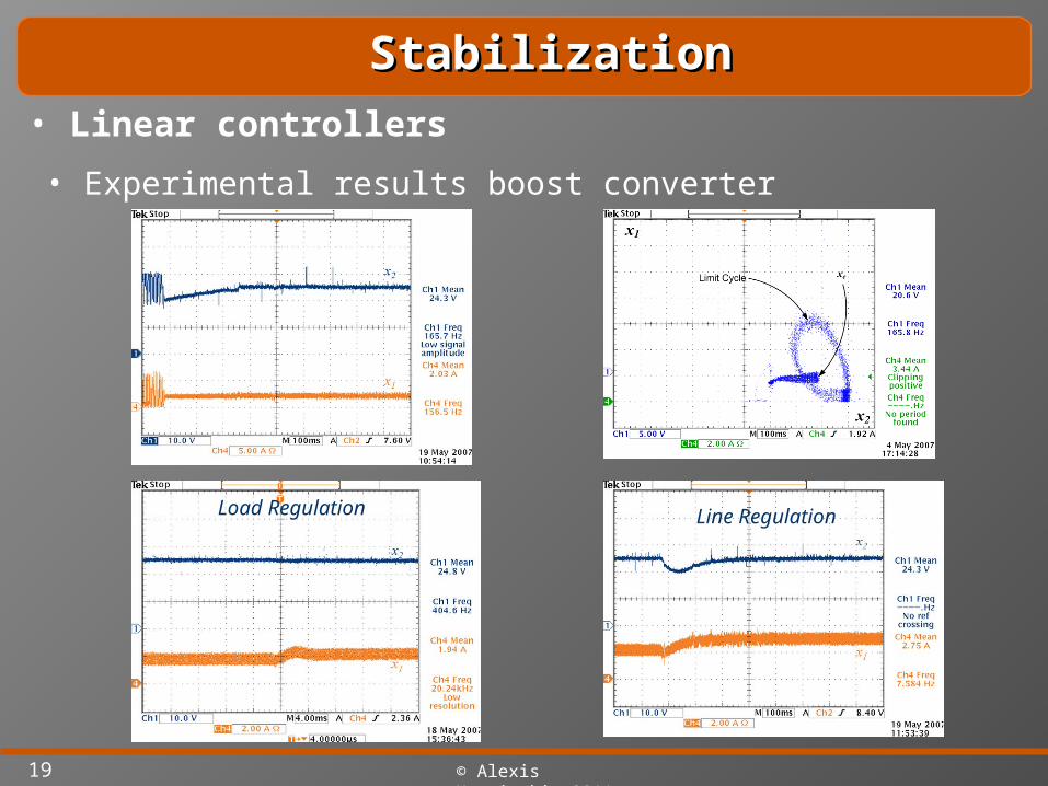
• Experimental results (buck converter)
• Linear controllers

14 © Alexis Kwasinski, 2011
StabilizationStabilization
• Experimental results (buck converter)
• Linear controllers
Line regulation
Load regulation

15 © Alexis Kwasinski, 2011
2 1
0 2
1' ' 4
' 1 ,2
i
i
RD D Ce e
V Rd d
• Linear controllers – Passivity based analysis
StabilizationStabilization
• The same analysis can be performed for boost and buck-boost converters yielding, respectively
2
1 2 02
0 0 0 2
4( ) ( )
'2
i
i
R x VE ECx
V E V E V E Rd
• Engineering criteria dictate that the non-linear PD controller can be translated into an equivalent linear PD controller of the form:
' 'd pd k e k e D
max max,
max
max
min ' '( , )
subject to 0 1
0 1
p de e e e
d d k k
d d
d d
• Formal analytical solution:
16 © Alexis Kwasinski, 2011
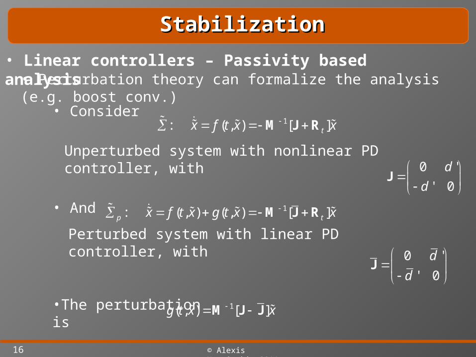
• Consider
• And
•The perturbation is
1: ( , ) [ ]tx f t x x M J R
1: ( , ) ( , ) [ ]p tx f t x g t x x M J R
1( , ) [ ]g t x x M J J
0 '
' 0
d
d
J
0 '
' 0
d
d
J
Unperturbed system with nonlinear PD controller, with
Perturbed system with linear PD controller, with
• Linear controllers – Passivity based analysis
StabilizationStabilization
• Perturbation theory can formalize the analysis (e.g. boost conv.)
17 © Alexis Kwasinski, 2011
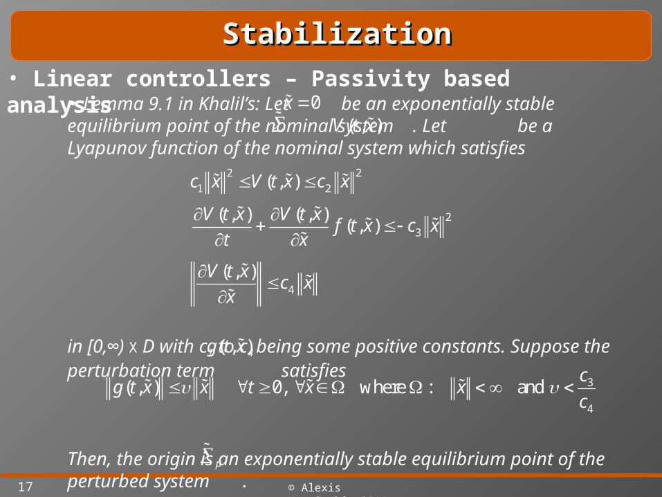
• Lemma 9.1 in Khalil’s: Let be an exponentially stable equilibrium point of the nominal system . Let be a Lyapunov function of the nominal system which satisfies
in [0,∞) X D with c1 to c4 being some positive constants. Suppose the perturbation term satisfies
Then, the origin is an exponentially stable equilibrium point of the perturbed system .
0x ( , )V t x
2 2
1 2( , )c x V t x c x
2
3
( , ) ( , )( , )
V t x V t xf t x c x
t x
4
( , )V t xc x
x
( , )g t x
3
4
( , ) 0, where : and c
g t x x t x xc
p
• Linear controllers – Passivity based analysis
StabilizationStabilization

18 © Alexis Kwasinski, 2011
•Taking•It can be shown that
•Also, is an exponentially stable equilibrium point of ,
and
with
•Thus, stability is ensured if
( , ) ( )V t x H x
c1 = λmin(M)
c2 = λmax(M)
3 min (2 3 )tc J R
( ' ') ( ' '),
d d d dmax
L C
G
(2 3 )' '
,
min td dC L
maxL C
J R
24 ( ) , ) , )T 2
maxc max(L C max(L C M M M
( , ) 0, where : g t x x t x x
0x ( ,0) 0g t
• Linear controllers – Passivity based analysis
StabilizationStabilization
19 © Alexis Kwasinski, 2011
Line RegulationLoad Regulation
StabilizationStabilization
• Experimental results boost converter
• Linear controllers

20 © Alexis Kwasinski, 2011
Line RegulationLoad Regulation
StabilizationStabilization
• Experimental results voltage step-down buck-boost converter
• Linear controllers

21 © Alexis Kwasinski, 2011
Line RegulationLoad Regulation
StabilizationStabilization
• Experimental results voltage step-up buck-boost converter
• Linear controllers

22 © Alexis Kwasinski, 2011
• All converters with CPLs can be stabilized with PD controllers (adds virtual damping resitances).
• An integral term can be added for line and load regulation
• Issues: Noise sensitivity and slow
StabilizationStabilization
• Linear Controllers - passivity-based analysis

23 © Alexis Kwasinski, 2011
• Boundary control: state-dependent switching (q = q(x)).
• Stable reflective behavior is desired.
• At the boundaries between different behavior regions trajectories are tangential to the boundary
• An hysteresis band is added to avoid chattering. This band contains the boundary.
StabilizationStabilization
• Boundary controllers

24 © Alexis Kwasinski, 2011
• Linear switching surface with a negative slope:
Switch is on below the boundary and off above the boundary
1 2 2 1( )OP OPx k x x x
StabilizationStabilization• Geometric controllers – 1st order boundary

25 © Alexis Kwasinski, 2011
• Switching behavior regions are found considering that trajectories are tangential at the regions boundaries.
• For ON trajectories:
• For OFF trajectories:
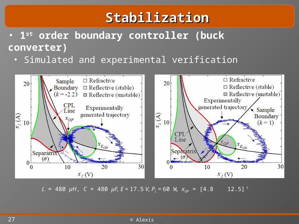
• 1st order boundary controller (buck converter)
1
2
1 11
2 2 2
x OP
x OP
f x xdxk
f dx x x
1 12
1 2 2 2
( )
( / )OP
L OP
x xC E x
L x P x x x
21 2 1 1 2 1 1
2 32 2 2 2 2
( ) : [ ] [ ( ) ] 0
ON OP L L OP
OP OP
x L x x x x x P x P xC Ex x E x x x
1 12
1 2 2 2
( )
( / )OP
L OP
x xC x
L x P x x x
2 2 31 2 1 1 2 1 1 2 2 2( ) : [ ] [ ] 0OFF OP L L OP OPx L x x x x x P x P x C x x x
StabilizationStabilization

26 © Alexis Kwasinski, 2011
2( ) 0
2 OP
CV x x x 2
2 2 12
( ) (1 )( )OP
LPV x k x x x
x
• Lyapunov is used to determine stable and unstable reflective regions. This analysis identifies the need for k < 0
• 1st order boundary controller (buck converter)
StabilizationStabilization
27 © Alexis Kwasinski, 2011
StabilizationStabilization
• Simulated and experimental verification
• 1st order boundary controller (buck converter)
L = 480 µH, C = 480 µF, E = 17.5 V, PL = 60 W, xOP = [4.8 12.5] T

28 © Alexis Kwasinski, 2011
StabilizationStabilization
• Simulated and experimental verification
• 1st order boundary controller (buck converter)
Buck converter with L = 500 μH, C = 1 mF, E = 22.2 V, PL = 108 W, k = –1, xOP = [6
18] T

29 © Alexis Kwasinski, 2011
Line regulation: ∆E = +10V (57%)
Load regulation: ∆PL = +20W (+29.3%) No regulation: ∆PL = +45W (+75%) Load regulation: ∆PL = +45W (+75%)
Line regulation: ∆E = +10V (57%)
StabilizationStabilization
• Line regulation is unnecessary. Load regulation based on moving boundary• 1st order boundary controller (buck converter)
30 © Alexis Kwasinski, 2011
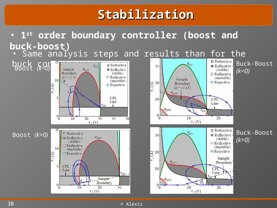
StabilizationStabilization
• Same analysis steps and results than for the buck converter.
• 1st order boundary controller (boost and buck-boost)
Boost (k<0)
Boost (k>0)
Buck-Boost (k<0)
Buck-Boost (k>0)

31 © Alexis Kwasinski, 2011
StabilizationStabilization
• Experimental results.
• 1st order boundary controller (boost and buck-boost)
Boost (k<0)
Boost (k>0)
Buck-Boost (k<0)
Buck-Boost (k>0)

32 © Alexis Kwasinski, 2011
StabilizationStabilization
• Experimental results for line and load regulation
• 1st order boundary controller (boost and buck-boost)
Boost: Load regulation
Boost: Line regulation
Buck-Boost: Load regulation
Buck-Boost: Line regulation

33 © Alexis Kwasinski, 2011
• First order boundary with a negative slope is valid for all types of basic converter topologies.
• Advantages: Robust, fast dynamic response, easy to implement .
• Geometric controllers
StabilizationStabilization