1 AD-A146 018 A COMPARATIVE STUDY OF THE FINITE ELEMENT AND BOUNDARY IlELEMENT METHODS AS..U) AERONAUTICAL RESEARCH LABS

U CMELBOURNE (AUSTBALIA) I AN CONG APR 84UNCLASSIFIED ABL-AEBO-TM-363 F/ 12/ 2IE

1111 1.04

MICROCCOY RE 'ION TEST CHART%A O 06A RE A, ANDARDS -'-963 -

A&L-AW--363 AR-003-024

DEPARTMENT OF DEFENCE

S DEFENCE SCIENCE AND TECHNOLOGY ORGANISATION

AERONAUTICAL RESEARCH LABORATORIESI MELBOURNE, VICTORIA

0

Amrodynamics Technical mesiwndum 363

A COMPARATIVE STUDY OF THE FINITE ELEWNET AND BOUNDARY

ELEMENT METHODS AS APPLIED TO A BOIUNDARY VALUEPROBLEM OF A HARMOIIC FUNCTION

T Iil. tlTErF ZTArES NATIONAX L

TON TRA ,N-CONG I TEcHNtCAL INFrRMATION SRVICE

S T AtHC'IED TOREPRoDUCE AND SELL THIS REPORT

C:I Approved for Public Release

LU-- DTIC!z IELFCTE

C SEP'" 7 49B4

(C) CommKUanTU OF AUSTRAIA 1984 E

COPY No £1 1964

UNCLASSJED0 9 25 020

AR-003-024

DEPARTMENT OF DEFENCE

DEFENCE SCIENCE AND TECHNOLOGY ORGANISATION

AERONAUTICAL RESEARCH LABORATORIES

Aerodynamics Technical Memorandum 363

A COMPARATIVE STUDY OF THE FINITE ELEMENT AND BOUNDARYELEMENT METHODS AS APPLIED TO A BOUNDARY VALUE

PROBLEM OF A HARMONIC FUNCTION

by

TON TRAN-CONG

SUMMARY

The Finite Element and Boundary Element Methods aredescribed with their essential features illustrated using an exampleof a boundary value problem for a harmonic function. Analysis ofthe methodical errors is then carried out. This is followed by aconsideration of the relative computational advantages of the twomethods. I

©COMMONWEALTH OF AUSTRALIA 1984

POSTAL ADDRESS: Director, Aeronautical Research Laboratories,P.O. Box 4331, Melbourne, Victoria, 3001, Australia

CONTENTS

PAGE NO.

1. INTRODUCTION 1

2. FORMULATION OF THE FINITE ELEMENT METHOD 1

3. FORMULATION OF THE BOUNDARY ELEMENT METHOD 4

4. ERROR ANALYSIS FOR THE BOUNDARY AND FINITE 6ELEMENT METHODS

4.1 Boundary Element Method 6

4.2 Finite Element Method 7

5. RELATIVE COMPUTATIONAL ADVANTAGES OF FINITE AND 9AND BOUNDARY ELEIENT METHOD AS FOR THE TESTPROBLEM

6. FINAL REMARKS 9

REFERENCES

FIGURE

APPENDIX: Convergence of Gauss-Seidel Method for PositiveDefinite Hermitian Matrices

DISTRIBUTION LIST

DOCUMENT CONTROL DATA

LAccession For

NTIS GA&DTIC TAB1JUnnnouncedJustificatio

By-Distribution/

Availability Codes t

Avall and/orDst !Special .

[1]

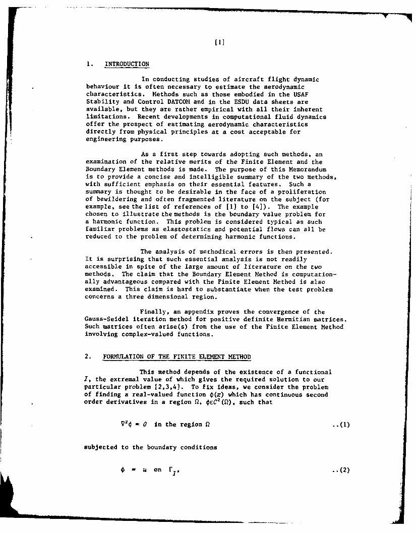
I. INTRODUCTION

In conducting studies of aircraft flight dynamicbehaviour it is often necessary to estimate the aerodynamiccharacteristics. Methods such as those embodied in the USAFStability and Control DATCOM and in the ESDU data sheets areavailable, but they are rather empirical with all their inherentlimitations. Recent developments in computational fluid dynamicsoffer the prospect of estimating aerodynamic characteristicsdirectly from physical principles at a cost acceptable forengineering purposes.

As a first step towards adopting such methods, anexamination of the relative merits of the Finite Element and theBoundary Element methods is made. The purpose of this Memorandumis to provide a concise and intelligible summary of the two methods,with sufficient emphasis on their essential features. Such asummary is thought to be desirable in the face of a proliferationof bewildering and often fragmented literature on the subject (forexample, see the list of references of [1] to [4]). The examplechosen to illustrate the methods is the boundary value problem fora harmonic function. This problem is considered typical as suchfamiliar problems as elastostatics and potential flows can all bereduced to the problem of determining harmonic functions.

The analysis of methodical errors is then presented.It is surprising that such essential analysis is not readilyaccessible in spite of the large amount of literature on the twomethods. The claim that the Boundary Element Method is computation-ally advantageous compared with the Finite Element Method is alsoexamined. This claim is hard to substantiate when the test problemconcerns a three dimensional region.

Finally, an appendix proves the convergence of theGauss-Seidel iteration method for positive definite Hermitian matrices.Such matrices often arise(s) from the use of the Finite Element Methodinvolving complex-valued functions.

2. FORMULATION OF THE FINITE ELEMENT METHOD

This method depends of the existence of a functionalI, the extremal value of which gives the required solution to ourparticular problem 12,3,4]. To fix ideas, we consider the problemof finding a real-valued function (x) which has continuous secondorder derivatives in a region S2, 4cC 2 (Q), such that

V2 - 0 In the region 0 ..()

subjected to the boundary conditions

* - u on r1, ..(2)

[21

on r2

where the two disjoint surfaces r and r form the boundary r of theregion 2. (The region 0 and its ioundary r are such that all class-ical theorems of calculus are applicable). It is straightforward touse the divergence theorem to prove that the above problem has onlyone solution 0(T). When r = r1 the above boundary value problembecomes the Dirichlet problem and when r r2, the Neumann problem(only in this latter case *(T) is determined only up to a constant).Here we take for granted that there exists a solution O(x) to theabove boundary value problem.

Let us form the functional

I() J ,V -2 .. (4

where p = p2 on F2 and p = 0 on F 1inimization of this functionalI with respect to q(x) such that u on r1 gives

0= J 6o v2¢ + 60 ( p

for any arbitrary incremental function 60 t CE2(.) satisfying 60 = 0on F.. Hence, instead of solving for 4 satisfying the system ofequalions {(I), (2), (3)} we can minimize (4) subjected to thecondition (2). This is the basis for the Finite Element Method.

Thus the Finite Element Method replaces the functionC £ C2(S2) by an approximation function 4(x) which is determined by

a finite number of its nodal values $(x ), m = 1, N inside 02. Thesem

nodal values are determined by the minimization of 1(4). The non-nodal values '(x) are determined from the N nodal values so obtained.In all the following, the function D(x) in each elemental volume willbe a linear interpolation of its nodal values at the vertices of theelement, as a result, the function 4D(x) satisfies V24)= 0 within eachelemental volume but not across inter-element boundaries (the higherorder inter~olation of ¢(x) does not automatically satisfy thecondition V 0 - 0 within each element and additional equations areimposed as a result).

The functional 1(4)) is now discretized into

1(4)) JV1 + E I y4'1VIi V.2 U V. V.

2 p - 2Ep

F-(y 1 Uy2 ) Yi

as in Figure 1.

[3]

Since 4(x) within each elemental volume can not beaffected by any nodal values outside the element, we have theequations determining t(x M) as in the following:

For a node a inside S, i.e. not on the boundaryr2 ,1

? (real constant depending only on the0 f E geometry of (a 3 a23 a3c 4 j c 6,a7 ) ) a aa)

For a node a3 on the boundary r2,

pa ~ ~ 3~ Kreal constant depending only on 1a3 i=l 2,3 4 (the geometry of (a3,a2 3a1,o4) a .

For typical nodes a2 , a7 belonging to the boundary

Ua2 a2

u = *.. (9)a7 a 7

All equations of the kind (7), (8), (9) form a largesystem of n equations in n unknowns. The function 0(T) is consideredknown when its approximation 4(x) can be shown to be reasonably closeto it.

The right hand sides of equations (7) and (8) resultfrom the differentiation of a homogeneous second degree polynomialin (P Therefore, we have

N[E a. IV JI 2 - 2 IVy)12 > oz ~ , I v0i=1 1i ¢: J ~

Hence the matrix A of coefficients in the equations (7), (8) and (9)satisfies

4 A € 0 , ..(10)a. CL Ct. a.

and is positive definite (it is easy to show that A is also symmetric).The Gauss-Seidel iteration method can thus be used to advantage insolving for the unknowns of the system {(7),(8),(9)}, see theappendix at the end of the memo.

[4]

The calculations in this section also hold if thefunction i(x) is complex-valued. In this case the last integralof equation (4) changes to Real (Ir0 p) where p is the complexconjugate of p, the matrix A of equation (10) becomes a positivedefinite Hermitian matrix, also equations (5) and (6) changeslightly but this does not alter our final system {(7),(8),(9)}.

3. FORMULATION OF THE BOUNDARY ELEMENT METHOD

To solve for the solution of the same system {(1),(2),(3)} the Boundary Element Method starts with the identity

J (V20) y = 0

where y is any C2(S) function. Using Green's theorem to integratethe above integral by parts, we have

€ (V22Y) - 2L + o -E"F F

Letting V2y= -6(,-_ *) where x* is on the boundary Fof the region 0, we have the following singular equation

Y 0 (.*) + 0 2Y- J !;L . 0 .. (13)

Jr- S(x*) an - s(x*) a

where S(x*) is a very small sphere centered on x* E F and y is aconstant equal to the fraction of the surface of S(x*) containedin P; when F is smooth this ratio Y is equal to one half.

The function 0 EC 2 (p) is now approximated by afunction '(;) which is determined by its nodal values 'V(x ),rn-1, M on the boundary F. The function T is harmonic and itsvalue on each elemental boundary element can be taken to beconstant or the interpolation between the nodal values at thevertices of the (boundary) element. The equations determiningthe nodal values of T are thus

-Y ~ ~ ~ nr.+Ej=1 ) + £ b ) n j=l "Jr-S(c. )

where yi(X) is given by

[5]

Yi (X) 1 i=1,...M. ..(15)

411 F7- I

In any case the equations (14) have only M unknownssince either (x.) or 3 is known for a given node.

-. (X d

For nodes x. on ri , we have

G (X-) = H..i'(x.) " i = 1'...m.

For nodes x. on r2

Hij T(X2).3 =a l (x) i = Al + 1,...,M.

The unknows on the right hand side of equations (16)are then solved and the value of '(x) at any interior point a of2 is easily worked out using equation (12) with V2y= -6(x- a).

Note that the approximation function '(x) so derivedsatisfies equation (1) everywhere but satisfies the boundary conditions(2) and (3) only at ! points. In other words, equation (11) is alwayssatisfied inside P with i(x) while equation (13) on the boundary F,which should also be satisfied identically for every singular functionZ(X) = 1/Ix-x*I, x*E F, is satisfied for only I functions y (x)defined by equation (15). For this reason the method has beenconsidered by some authors a weighted residual method, meaning thatequation (13) is satisfied only for a finite number (M, in this case)of weighting functions .i(x).

It is now obvious that the Boundary Element Methoddepends on the use of Green's identity

(a 2b - ;-V2a) _ - - ..(17)

although the usual approach using the weighted residual method oftendisguises this under the process of partial integrations. Anotherinteresting feature of the Boundary Element Method is the applicabilityof the Maximal Value Theorem which states that a harmonic functionattains its maximal values only on the boundary [5]. The value ofthe methodical error k¢(x) - i(x)I at an interior point of S is thusalways less than such value at some point on the boundary r and thelatter can be reduced with a finer discretization of r.

IT.

[6]

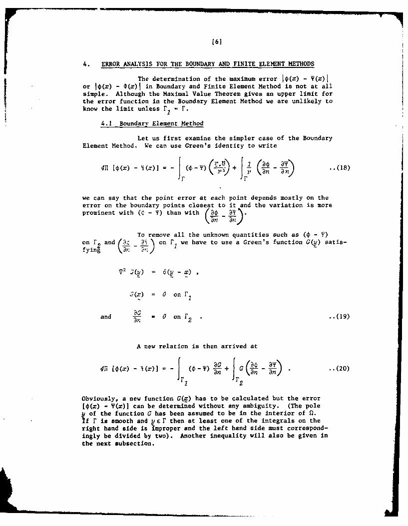
4. ERROR ANALYSIS FOR THE BOUNDARY AND FINITE ELEMENT METHODS

The determination of the maximum error J (X) - Y(X)lor 10(x) - 4(x) in Boundary and Finite Element Method is not at all

simple. Although the Maximal Value Theorem gives an upper limit forthe error function in the Boundary Element Method we are unlikely toknow the limit unless ri = r.

4.1 Boundar" Element Method

Let us first examine the simpler case of the BoundaryElement Method. We can use Green's identity to write

411 [4(x) - 1(x)] = - (4 - Y) (- + .1 - . (18)

we can say that the point error at each point depends mostly on theerror on the boundary points closest to it and the variation is moreprominent with ( - )than with 4 _ _ l, .

On an2

To remove all the unknown quantities such as (0 - T)on fr 2 and ( €'1\ on r we have to use a Green's function G(y) satis-

fying On C

V2 3(Y) = 6(y -x)

S7x) = 0 on r

and 4G 0 onF 2 F.(19)

A new relation is then arrived at

411 [O(x) - 4(x)] = - ( y) L + G (. a Y..(20)rI F2

Obviously, a new function G(x) has to be calculated but the error

[4(x) - P(x)] can be determined without any ambiguity. (The poley of the function G has been assumed to be in the interior of S2.

If r is smooth and y e r then at least one of the integrals on theright hand side is Improper and the left hand side must correspond-ingly be divided by two). Another inequality will also be given inthe next subsection.

[7]

4.2 Finite Element Method

The estimation of error for the Finite Element Methodis more complicated as we have here in addition to the interpolationerror on the boundary another kind of error arising from the dis-cretization of the function 4)(x). This makes its gradient W) varyin a stepwise manner within Q ind the jumps occur at inter-elementboundaries. The Maximal Value Theorem is not applicable in thiscase as € is not harmonic over the region Rt.

A natural way to measure the closeness of O(x) to¢(x) is to use the difference

.1(0)-'(€) ' IyJ 2 - Iy4)12)- 2J (4' -4)) p. .. (21)

Hence

1() - IC)=2f V' (-)-J [ V(4-) ]2

- (4- 4) p ..(22)

Hence to have more accurate results we must makeU- €) small especially when V is large and similarly for (0 - 4)

on the boundary, it must be small where p is large.

Similarly to the case of Boundary Element Method, theerror in Finite Element Method can be written down as

411 [(x) - t (x) I -G (I-I ta+ - -L - JG -L4 .. (23)rIJr r 2 s

where G is the Green's function defined by equation (19) and S is asurface comprised of the double layers enclosing all inter-elementboundaries with the normals pointing away from the elemental volumes.The equation holds for any point x interior to Q. If x is right onthe boundary T then at least one 6f the first two integrals on theright hand side of (23) is improper and also the left hand side mustbe divided by two. The last integral in equation (23) is the errorcaused by the stepvise variation of VO. Therefore, the errors(4 - ) and( on r and r' iespectively, as well as they1 2jump in VW across inter-element boundaries must all be reduced if wewant to reduce the magnitude of the left hand side of (23).

[81

An often suggested measurement for the global performance(i.e. performance over the whole region n in an average manner) of aFinite Element scheme is the functional J defined by

i 1 - 2i 1 ..(24)

In the following we will examine the usefulness of this functional.

From equations (23) and (24) we have an inequality

It(t) -he(X) < C L 1 + IG12 i ..(25)is n an jr

which gives the upper bound for the point error [O(x) - 4)(x)] in

terms of J and the Green's function defined by e' on (19). Itis obvious that even if we are only concerned wi the resultingvalues of €(x) and ¢(x) on the boundary r for a :titular FiniteElement scheme, the error originating from inte lement discontin-uities in V¢ still has to be accounted for. He _e ,e performanceof the scheme can not be adequately measured by - use of J alone.

On the other hand, if we omit the first term on theright hand side of equation (25) and replace O(x) by (x) we havean inequality for the Boundary Element Method. -Hence J~is a goodmeasurement of the global performance of any Boundary Element scheme.

J can also be related to the quantity [1(0) - IM)

by derivation from equations (21) and (24). We get

(0) -( (0-) 2i +

J + + I -€ 12 ..(26)

The first integral is the effect of the jump in V4across inter-element boundaries and the last integral becomes negligiblewhen 0 is close to €.

In a similar way we also have

[I '(4') - '(c I {J I 4- * IV + JI * - * IJ *

ft ris' i 0 1n+ + + J- p 12 ..(27)

Is r1 1 r

[9]

which shows the effect of J$ - 01 on the difference I(0) - I(o).

5. RELATIVE COMPUTATIONAL ADVANTAGES OF FINITE AND BOUNDARYELEMENT METHOD AS FOR THE TEST PROBLEM

The case where the region 2 is one dimensional ismuch too simple to have any significance. Therefore, only thecases where Q is two or three-dimensional are considered.

First when 2 is two-dimensional the FEM (FiniteElement Method) has n2 nodes and requires n2 memory locations. Incontrast, the BEM (Boundary Element Method) requires only n nodesbut also n2 memory locations. If the Gauss-Seidel iterative methodis used for the banded matrix of the FEM and the standard Doolittleor Gaussian method is used for the full natrix of the BEM then theircomputing time will be proportional to n and n3 respectively. Thusthe BEM is advantageous in this case.

On the other hand, when . is three-dimensional, theFENM and B-N requre(s) n3 and n2 nodes respectively. Memory locationsrequired are of order n3 and n4 respectively and the computing timesare the same. Thus, the FEM is advantageous in this case.

6. FINAL REM.ARKS

Besides those points considered in the previous section,others which favours one method over the other are:

(i) The gradient of q(x) is approximated by step-like functionV, in FEI compared to a harmonic function VT in BEM.

(ii) The setting up of a BEM program requires some elaboratecalculation for each singular component of the surfaceintegral. This is in direct contrast with the straight-forward setting up procedure of FEM. Moreover, the valuesof the integrals in BEM are fairly sensitive to theaccuracy of the integration near to their singularities.This creates yet another kind of error which has to beconsidered.

(iii) For problems with a non-homogenous body the BEM requiresa subdivision of the body while FEM has this featureinherent in it.

(iv) With any subdivision of a body such as in (iii) or as fora long a narrow region (for example, see [1], p. 183) theBEM becomes a hybrid between itself and the FEM. Mixedcharacters can thus be expected in this case : For examplt,the coefficient matrix becomes slightly banded and thefunction Y(T) is not harmonic at all interior point of theregion f?.

[101

(v) The truncation error in the Gauss-Seidel iteration forthe FEU is usually of greater order of magnitude thanthe round off error. The latter also does not improvemuch with the use of internal double precision in itsequation solving subroutine.

AW

REFERENCES

[1] Brebbia, C.A. The Boundary Element Method forEngineers.Pentech Press, 1978.

[21 Zienkiewics, O.C. The Finite Element Method inEngineering Science.

McGraw-Hill, 1971.

[31 Shen, Shan-fu Finite Element Methods in FluidMechanics.

Ann. Rev. Fluid Mech., 1977.

[4] Thomasset, F. Implementation of Finite ElementMethods for Navier-Stokes Equations.Springer-Verlag, 1981.

[51 Rabenstein, A.L. Introduction to Ordinary DifferentialEquations.

Academic Press, 1972.

[6] Varga, R.S. Matrix Iterative Analysis.Prentice-Hall, 1962.

[7] Ralson, A. and A first Course in Numerical Analysis.Rabinowitz, P. McGraw-Hill, 1978.

6 7

cx2p a17 c y, cr

S2'f 3' a 4 cy2 Uv 3 cF 2

FIG. 1 DISCRETIZATION OF A REGION f,AND ITS BOUNDARY r

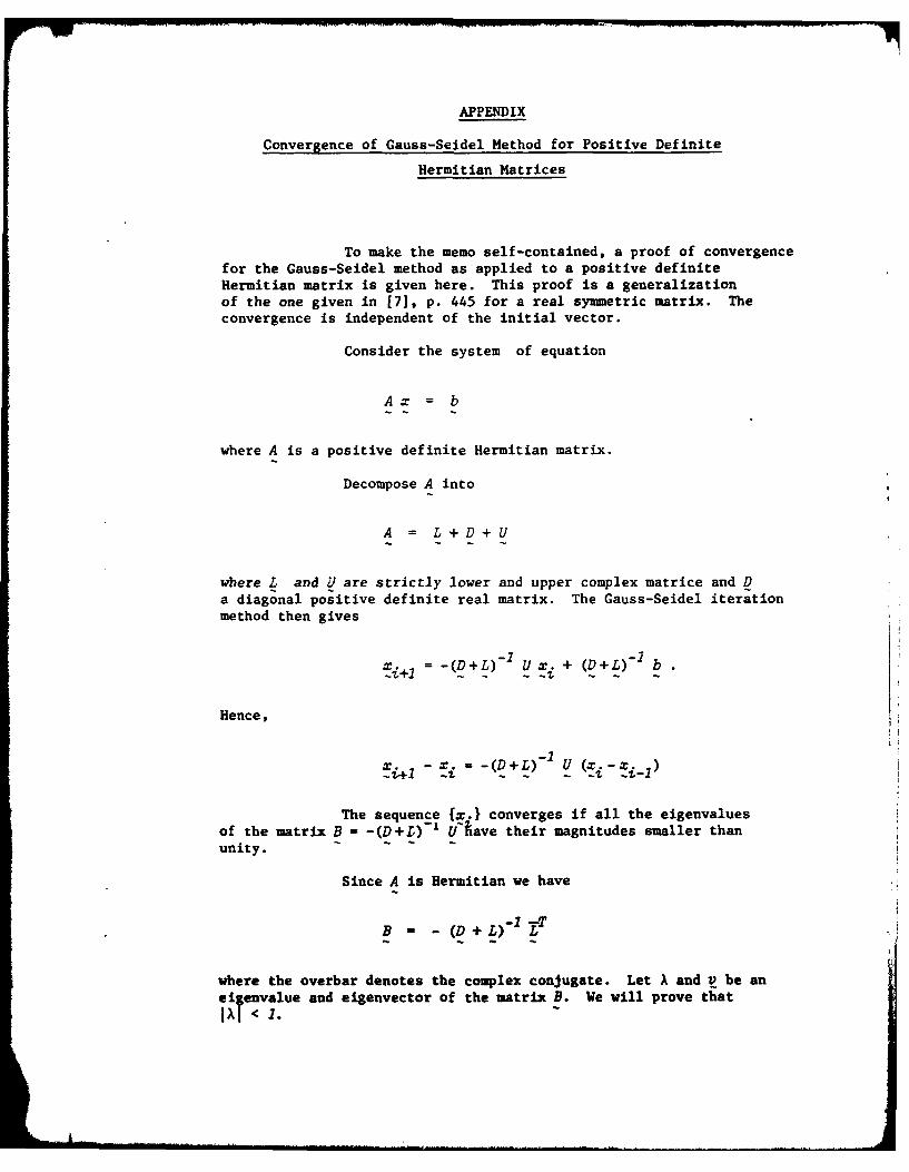
APPENDIX

Convergence of Gauss-Seidel Method for Positive Definite

Hermitian Matrices

To make the memo self-contained, a proof of convergencefor the Gauss-Seidel method as applied to a positive definiteHermitian matrix is given here. This proof is a generalizationof the one given in [7), p. 445 for a real symmetric matrix. Theconvergence is independent of the initial vector.

Consider the system of equation

Ax = b

where A is a positive definite Hermitian matrix.

Decompose A into

A = L+D+U

where L and 1' are strictly lower and upper complex matrice and Da diagonal positive definite real matrix. The Gauss-Seidel iterationmethod then gives

. = -(D+L) U .I + (D+L)- I b.

Hence,

X. x. = _D+L) - U (x.- x_

The sequence {x.} converges if all the eigenvaluesof the matrix B - -(D+L)-' Uliave their magnitudes smaller thanunity. ~

Since A is Hermitian we have

-2 -=TB = -(D+ L) L-

where the overbar denotes the complex conjugate. Let A and v be anei envalue and eigenvector of the matrix B. We will prove thatIX/ < 2.

A.2

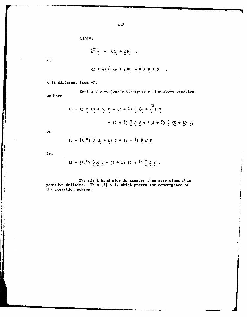
Since,

-=T

L A - (D +L)V

or

(2 +A) (D+ L)v =VA v > 0

X is different from -1.

Taking the conjugate transpose of the above equationwe have

(1 + X) v (D + L) v - (1 + A) v (D + LT) V

S(1 + 1) V DV + X(l + 1) V (D + L) V,

or

(2- IX2) (D + L) - (1 + A) V D V

So,

(1- I2) v A v (1 + X) (1,) + D V

The right hand side is greater than zero since D ispositive definite. Thus JXJ < 1, which proves the convergence-ofthe iteration scheme.

DISTRIBUTION

AUSTRALIA

Department of Defence

Central Office

Chief Defence Scientist )Deputy Chief Defence Scientist (copy)Superintendent, Science and Technology Programmes )Controller, Projects and Analytical Studies )Defence Science Adviser (U.K.) (Doc Data sheet only)

Counsellor, Defence Science (U.S.A.) (Doc Data sheet only)Defence Science Representative (Bangkok)

Defence Central LibraryDocument Exchange Centre, D.I.S.B. (18 copies)Joint Intelligence Organisation

Librarian H Block, Victoria Barracks, Melbourne

Director General - Army Development (NSO) (4 copies)

Aeronautical Research Laboratories

DirectorLibrarySuperintendent - AerodynamicsDivisional File - AerodynamicsAuthor: T. Tran-Cong (5 copies)D.A. SecombC.A. MartinP. HallJ.S. DrobikD. CollisR.A. Feik

R. JonesL.F. Rose

Materials Research Laboratories

Director/Library

Defence Research Centre

Library

RAN Research Laboratory

Library

Navy Office

Navy Scientific Adviser

Army Office

Army Scientific Adviser

... /cont.

DISTRIBUTION (CONT.)

Air Force Office

Air Force Scientific Adviser

Central Studies Establishment

Information Centre

Department of Defence Support

Government Aircraft Factories

Manager

Universities and Colleges

Sydney Dr G.P. Steven, Department of AeronauticalEngineering

SPARES (10 copies)

TOTAL (63 copies)

Department of Defence

DOCUMENT CONTROL DATA

1. e. AA No I. b rfisvk t No .. .. o;-bcu t Det 3.Yak No

AR-003-0247 ARL-AERO-TM-363 APRIL 1984 DST 82/030

A COMPARATIVE.STUDY OF THE FINITE ELEMENT " 14UNCLASSIFIED

AND BOUNDARY ELEMENT METHODS AS APPLIED TO b. the C. 6ct 7. NoA BOUNDARY VALUE PROBLEM OF A HARMONICFUNCTION U U 7BAuthorU) 9. Dradng Iuniong

TON TRAN-CONG

1o. c arm Au$, and A dd,, '1 Author it V ISp eapW.,lJ

Aeronautical Research Laboratories,P.O. Box 4331, -

MELBOURNE, VIC. 3001

I2. besonery Dmavanin tof tao amOuaI t

Approved for Public Release

ownews wQum o@qtde nwaed emthpols 2hou t b reterieo lroso ASDIS, Defenc Infovmation rorvamt Itonch, ,pennt of Deece. Cwpbe't Puuk. CANBERRA ACT 260113. a. mra docuw'e,! maf be AhNOUNCEO in etwovsd and evmremein meves *ailabv t.

No limitations.

13. k Cm. for @11w psrptn t Iemo enWnouamnm7:Jn mw be IgeerJ unnw"cedDtJ a few 13.14. 04004000. 15. COSATI GiFinite element analysisComparison 12010Error analysis 01010Boundary element methodBoundary value problem

W UAbM

- ... h The Finite Element and Boundary Element Methods aredescribed with their essential features illustrated using an exampleof a boundary value problem for a harmonic function. Analysis ofthe methodical errors is then carried out. This is followed by aconsideration of the relative computational advantages of the twomethods.

".

This op is to be usd to rcord information which is required by the Establishment for its own ue butwhich will not be Ord to the DISTIS da bm unls speclfImlly remqusd.

W . IunE Z J

Aeronautical Research Laboratories, Melbourne.

1f Dam n SU ad. 1W9Ud Is. Co st Caft p20. Type of , I Ort end Pw d Cowed~

Aerodynamics Technical 52 7730

Memorandum 363

21. Cemw Progwf Und

2. subbmmt Fo. PAfts)