1

DEMOGRAPHIC VARIABILITY IN U.S. CONSUMER RESPONSIVENESS TO CARBONATED SOFT-DRINK

MARKETING PRACTICES

Charles Rhodes

University of Connecticut

charlesrrhodes@gmail.com

2010

Copyright 2010 by Rhodes. All rights reserved. Readers may make verbatim copies of this document for non-commercial purposes by any means, provided that this copyright notice appears on all such copies.

Selected Paper prepared for presentation at the 1st Joint EAAE/AAEA Seminar

“The Economics of Food, Food Choice and Health”

Freising, Germany, September 15 – 17, 2010

2

Abstract Using three years of Nielson Homescan and advertising data from 16 major metropolitan areas across the U.S. to construct a panel data set that follows weekly consumer purchasing behavior, this paper investigates the impact of marketing activities on a representative cross-section of U.S. consumers. Because many consumers do not participate in the market week-in and week-out, I apply Heckman’s econometric selection model to recover the impact of pricing, advertising, and promotion on a wide range of consumer segments. Reduced-form estimates of consumer responsiveness to these marketing activities reveal different effects across consumer segments, which have numerous implications for marketing policy. Keywords: carbonated soft drink, marketing-mix models, demographic segmentation, econometric selection models, Nielsen panel data, food marketing policy JEL codes: D12, L66, M38

3

1. Introduction

The obesity epidemic in the United States has penetrated an increasing number of regions

and demographic groups over the last two decades, and seems to be going global (Popkin: 2004;

Yach, et al.: 2006). Diabetes rates are following. Nations that have enjoyed abundance now are

peopled by citizens who corporeally manifest superabundance to their own poor health

outcomes. Policy makers are taking increasing notice.

No one food group can plausibly be assigned causality, but we do know that sweetened

carbonated soft drinks (sCSDs) in the U.S. serve as pure vectors into the body of simple sugar

calories without fiber protein or any natural vitamin or mineral content to favor them

nutritionally. We further know that rising consumption of sCSDs in the U.S. has not only

paralleled the rise in obesity, but is highest among young adults (Binkley and Golub: 2007; Bray,

et. al.: 2004; Nielsen and Popkin: 2003). Who exactly is buying all of this colored high-fructose-

corn-syrup water, and are they that different from us? Does “Coke add life” for them? Are they

“Doing the Dew?” Are they motivated by multi-million dollar advertising campaigns, name

brand recognition going back generations, some of the cheapest calories in the supermarket, or

something else (Harris, et. al.: 2009)?

Recent academic access to an extremely rich marketing data set that spans the U.S.

allows the parsing of demographic correlations with sCSD purchase. I ask this data which

demographic groups have the largest marginal responses to changes in sCSD marketing

variables: price, discounting, and advertising (here called marketing mix variables).

Myriad sub-questions are enabled by the effort. Among them: What is the marginal effect

of an increase in household size on consumer response to discounting? Does purchase fall as the

formal education level of the head of household rises in comparative level? Do racial groups

with lower income profiles respond more in purchase to television advertising campaigns for

sCSDs than do racial groups who are characterized by higher mean household incomes?

The scope and characteristics of the data along with the focus of the question motivate

exploration of econometric modeling issues from within the modeling set for censored and

truncated data.

For my purposes here, let me define poor food choice to mean “unhealthful choice/a

choice that if regimented in individual consumption patterns is likely to lead to health problems

for an average individual.” Allow that the term “poor food choice” says nothing about poverty

(not “the poor”), or about the economically efficient or rational balance of expenditures of an

4

individual’s limited food budget (not “poor choice” in terms of utility maximization given a

budget constraint). Let me also define the term effective nutrition education to mean the level of

application of responsible nutritional choices in realized individual food/drink purchasing and

consumption patterns – e.g., a person who actually buys and consumes more carrots than candy

is demonstrating (a higher level of) effective nutrition education, i.e., more than someone who

buys and consumes more candy than carrots.

2. Literature Review

Relevant academic consideration of the use of demographic variables to determine brand

choice or market segment come from the Marketing literature. Chiang (1991), Kamakura and

Russell (1989), Gupta and Chintagunta (1994), and Kalyanam and Putler (1997) all develop

insights into the use of demographic variables as determinants of consumer choice. Fennell,

Allenby, Yang, & Edwards (2003) specifically study how demographic and psychographic

variables can be used to explain consumption rates and product use. They examine 52 product

categories, “providing evidence that these variables predict product use and unconditional brand

use, but do not predict brand choice conditional on product category use” (: 241). The fact that I

choose not to estimate demand (for reasons explained in section 4, see “RFM”), that my current

proposed estimation structure aggregates individual choice to the category (not brand) level, and

the fact that I will be using actual advertising exposure, separates this work from that of

predecessors I have so far identified, and suggests numerous points of potential separation or

extension from the existing literature.

Asking the data what correlations exist rather than building a structural model of demand

from economic theory is a methodological response motivated in part to findings from

behavioral economics focused on food consumption. These researchers discover consumer

behavior inconsistent with stated goals, inconsistent with stated perceptions, and divergent from

immediate memory of recent eating (Wansink: 2006). Rational maximization of utility may be a

process more rigorous than consuming a sCSD warrants (Just: 2010). Pesendorfer (:2006)

describes in his review of Advances in Behavioral Economics models of failures of expected

utility theory or hyperbolic discounting that may find appeal in application to marginal junk-food

consumption. Marginal junk-food consumption is likely to have a very attenuated negative

impact on health. Rational thinking about health impacts can easily be offset by rational thinking

about current utility maximization (“I’m hungry, and it’s here and cheap.”) Given this potential

5

conflict, it is inappropriate to presume that modes of consumer economic decision making about

junk-food purchases will be uniform.

Knowledge of proper nutrition in the U.S. is not extensive or impressive (Variyam and

Golan: 2002; Zamora and Popkin: 2007; Duffey and Popkin: 2006), so rational ignorance

(Downs: 1957) may also play into day-to-day consumption choices and habit formation. The

word “addiction” as applied to carbohydrate-intensive foods is beginning to be used in the

literature (Richards, et. al.: 2007). There may be real cumulative costs to habitual drinking of

sCSDs, but structural modeling tends to assume orderly preferences for even such attenuated

dangers, and that risks are unambiguously known and properly discounted by the individual. In

reality there are changing priorities and levels of awareness and responsibility playing out

dynamically in individual economic choices (Pesendorfer: 2006).

3. Data – Summarizing sCSD Consumer Markets

Data are from AC Nielson, weekly HomeScan, for three years from February 2006

through to December 2008 (152 weekly “Process Periods”), for 16 Designated Marketing Areas

(DMAs): Atlanta, Boston, Baltimore, Chicago, Detroit, Hartford & New Haven, Houston,

Kansas City, Los Angeles, Miami – Ft. Lauderdale, New York, Philadelphia, San Francisco –

Oakland – San Jose, Seattle – Tacoma, Springfield – Holyoke, and Washington D.C. DMAs are

defined by the range of metropolitan commercial television broadcast markets. This data set

combines specific purchase information, recorded after purchase by household members, with

the demographic information of the participating household.

Also from Nielsen are (television) advertising data corresponding to Nielson areas. These

are measured in population exposure to advertising within a broadcast market. This exposure is

measured in advertising-industry-standard units known as “gross rating points” (GRPs). Nielsen

categorizes the DMA-level GRPs to a certain level of demographic granularity (the entire data

set includes GRPs for specific-aged children, for example). After data management procedures,

13,356 households presented a balanced panel, for 358,518 purchase observations.

The research question of interest here is to examine the extent to which different

demographically identified groups respond to price, promotions/discounting, and advertising

(“marketing-mix”) variables. A dataset consisting of only purchase observations cannot directly

represent a choice not to purchase as a response to a price promotion or increased advertising. So

regressing on only positive observations with no other modeling correction would be a

6

misspecification for addressing this question. It is therefore necessary to balance the panel with

demographic information fully listed for “observations” in the weeks without purchase. The

integrity of the Nielsen data-gathering process ensures that these filled-in zeros are actual

purchase observations for the household for the week. This expands the ability of the existing

dataset to characterize real-world behavior. With every house exiting in the Nielsen panel during

a year now having an observation – zero or positive purchase – every week, the number of

observations rises to 2,003,644. With the filled-in zeros, non-purchase observations represent

81.2% of all observations.

Table 1 is a key the reader will find useful in explaining variable names, symbols, and

representational terms used in tables throughout the paper.

Table 1. Key to Variable Names, Symbols, and Their Meanings, Used in Later Tables

Variable Name Variable Meaning Notes

Demographic variables

HalfPov4Inc 0 to ½ x Pov4Inc Pov4Inc ≈ poverty-level x1Pov4Inc ½ to 1 x Pov4Inc income for U.S. family of 4

x2Pov4Inc 1 to 2 x Pov4Inc (U.S. average)

x3Pov4Inc 2 to 3 x Pov4Inc

x4Pov4Inc 3 to 4 x Pov4Inc

HHsiz2 Household Size = 2 members HH = Household

HHsiz3 Household Size = 3 members

HHsiz4 Household Size = 4 members

HHsiz5plus Household Size = 5 or more members

AfrAm African American

Asian Asian

OtherRace Other Race 62.5% identified Hispanic

Hispnc Hispanic separate from Race binaries

FemLessHSEdu Female best Educ level < high school ALL references to

FemHSEdu Female best Educ level = high school ‘Male’, ‘Mn’, or ‘M’ are for

FemSomCollgEdu Female best Educ level = some college Male head of household, with

FemCollgEdu Female best Educ level = full college ‘Fem’, ‘Fm’, or ‘F’ for Female

FemPostCollgEdu Female best Educ level = graduate work head of household;

MaleLessHSEdu Male best Educ level < high school head of household must be

MaleHSEdu Male best Educ level = high school M or F, but can be both

MaleSomCollgEdu Male best Educ level = some college MaleCollgEdu Male best Educ level = full college

MalePostColgEdu Male best Educ level = graduate work

MaleAgeL30 Male Age in years in category up to 29 “L” in any variable name

MaleAge30L40 Male Age in years between 30 & 39 means “less than”

MaleAge40L50 Male Age in years between 40 & 49

MaleAge50L65 Male Age in years between 50 & 64

MaleAge65plus Male Age in years 65 and older

7

FemAgeL30 Female Age in years in category up to 29

FemAge30L40 Female Age in years between 30 & 39

FemAge40L50 Female Age in years between 40 & 49

FemAge50L65 Female Age in years between 50 & 64

FemAge65plus Female Age in years 65 and older

FemUnderEmp Female Under-Employment <35 hrs/wk & Unemployed

ManNoEmp Male unemployed

ManNotFullEmp Male working <35 hrs/wk Other Variables

Ssn2 Summer (Apr-Jun)

Ssn3 Autumn (Jul-Sep)

Ssn4 Winter (Oct-Dec) ‘x’ anywhere after first character

Marketing & Interaction depicts interaction, no number

P, Sale , Adv Price index, Discount (Sale), Advertising on HHsiz depicts category, not

(e.g.) PxHHsiz price index interacted with HHsize level

HHTotOzByPP HH total oz purchased in a week the dependent variable

Table 2 shows summary statistics for marketing and purchase variables used in

regression. The dependent variable is a household’s weekly total ounces of sCSDs purchased.

Note that the standard deviation is over three times the mean in ounces. A price index of all soft

drinks purchased in a DMA shows an average price across the dataspan of 2.28 cents per ounce,

with standard deviation just over 10% of that value. Households typically buy a total of at least

67 oz. (2 liters or more) in a week an average of 8 times per year, but the standard deviation is

also just over 10% larger than the mean.

Table 2. Descriptive Statistics – Marketing and Purchase Variables

observations = 2,003,644 Variable Mean Std. Dev. Min Max Notes

Wkly HH Purchase Total (oz.) 49.396 165.984 0 12235.6 dependent variable Avg Price in $ in a DMA / wk 0.02280 0.00279 0.0108 0.0346 indexed for all sCSDs HH’s Purchase of 67 ozs. 8.021 9.251 0 52 # of Wks / Yr.

Discount - Sale 0.060 0.237 0 1

Discount - Coupon 0.011 0.105 0 1

HH Avg. Advert Exposure 171.977 126.209 2.752 748.196 DMA-level

Only six percent of purchases are bought “on sale” as logged by Nielsen participants, but

the standard deviation is four times this. “Coupon” is an extant method of price promotion,

making it a marketing mix variable, but it was dropped from the interaction set as a potentially

interesting driver of sub-sample behavior, as only 1% bought with couponing. Household

advertising exposure, in GRPs, has a standard deviation roughly 75% of its mean value.

8

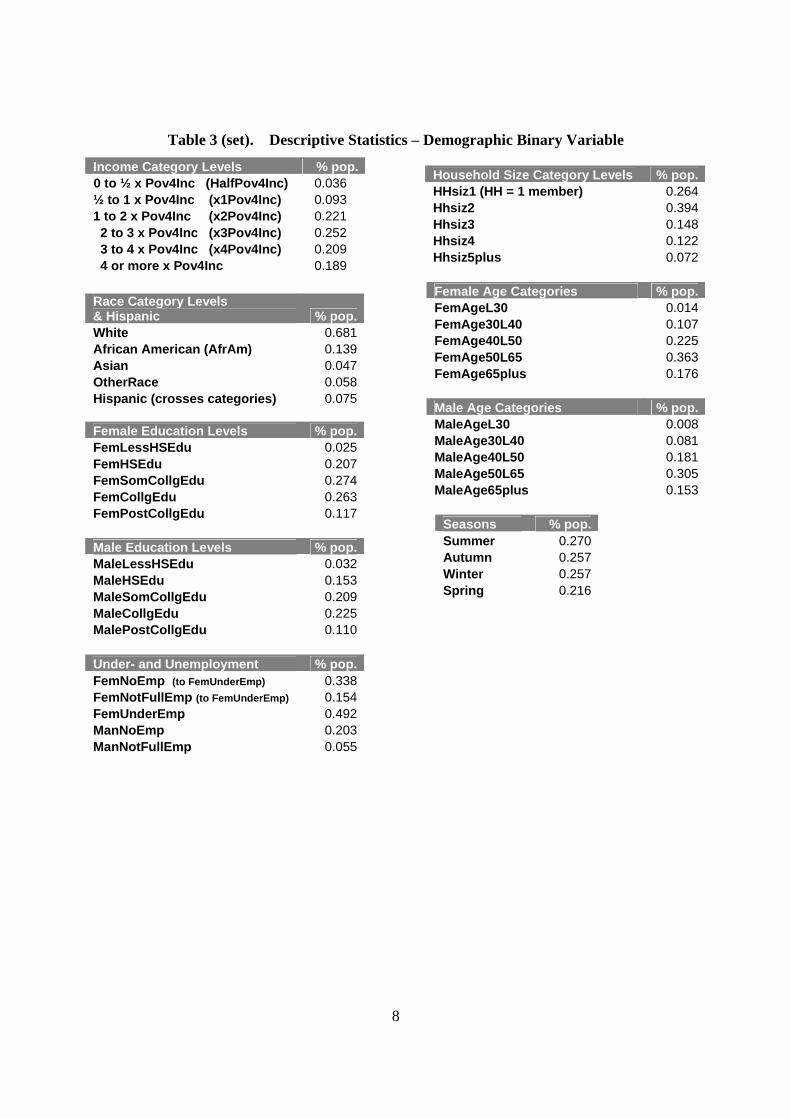
Table 3 (set). Descriptive Statistics – Demographic Binary Variable

Income Category Levels % pop.0 to ½ x Pov4Inc (HalfPov4Inc) 0.036 ½ to 1 x Pov4Inc (x1Pov4Inc) 0.093 1 to 2 x Pov4Inc (x2Pov4Inc) 0.221 2 to 3 x Pov4Inc (x3Pov4Inc) 0.252 3 to 4 x Pov4Inc (x4Pov4Inc) 0.209

4 or more x Pov4Inc 0.189

Race Category Levels & Hispanic % pop.White 0.681African American (AfrAm) 0.139Asian 0.047OtherRace 0.058Hispanic (crosses categories) 0.075

Female Education Levels % pop.FemLessHSEdu 0.025FemHSEdu 0.207FemSomCollgEdu 0.274FemCollgEdu 0.263FemPostCollgEdu 0.117

Male Education Levels % pop.MaleLessHSEdu 0.032MaleHSEdu 0.153MaleSomCollgEdu 0.209MaleCollgEdu 0.225MalePostCollgEdu 0.110

Female Age Categories % pop.FemAgeL30 0.014FemAge30L40 0.107FemAge40L50 0.225FemAge50L65 0.363FemAge65plus 0.176

Under- and Unemployment % pop.FemNoEmp (to FemUnderEmp) 0.338FemNotFullEmp (to FemUnderEmp) 0.154FemUnderEmp 0.492ManNoEmp 0.203ManNotFullEmp 0.055

Household Size Category Levels % pop.HHsiz1 (HH = 1 member) 0.264Hhsiz2 0.394Hhsiz3 0.148Hhsiz4 0.122Hhsiz5plus 0.072

Male Age Categories % pop.MaleAgeL30 0.008MaleAge30L40 0.081MaleAge40L50 0.181MaleAge50L65 0.305MaleAge65plus 0.153

Seasons % pop. Summer 0.270 Autumn 0.257 Winter 0.257 Spring 0.216

Table 3 (a set of smaller tables), presents demographic variables at chosen levels, each

parsed from categoric variables. For example, income is presented as a single variable in the raw

dataset, with 27 possible incremental values, from which five levels are presented here (using a

fifth, the highest, as a control). The size of the data enables this foray into granularity, risking

insignificant standard errors in the estimation process. The percentages presented for each

demographic category level represent that category level’s percentage representation of the entire

category.

The Race category, presents an exception, as “Hispanic” is a self-defined category that

overlaps the four groups included in the Race category. While Hispanic crossovers to the White,

African-American, and Asian categories can be clearly identified, the only way to self-identify as

Hispanic only is to choose “Other Race” and the Hispanic identification dummy. Checking data

not presented here, one finds 62.5% of those selecting “Other Race” identify as Hispanic. Thus

roughly 40% of the 7.5% of the sample identified as Hispanic in Table 1 are spread over the

White, African-American, and Asian “levels.” Table 4 in part demonstrates how this ambiguity

manifests.

Returning to Table 3, for the income, and male and female age and education levels, the

lowest value is not represented by more than 3.6% of the sample. With relatively few relatively

time-invariant observations for certain levels, there may be constraints on statistical significance

in the analysis.

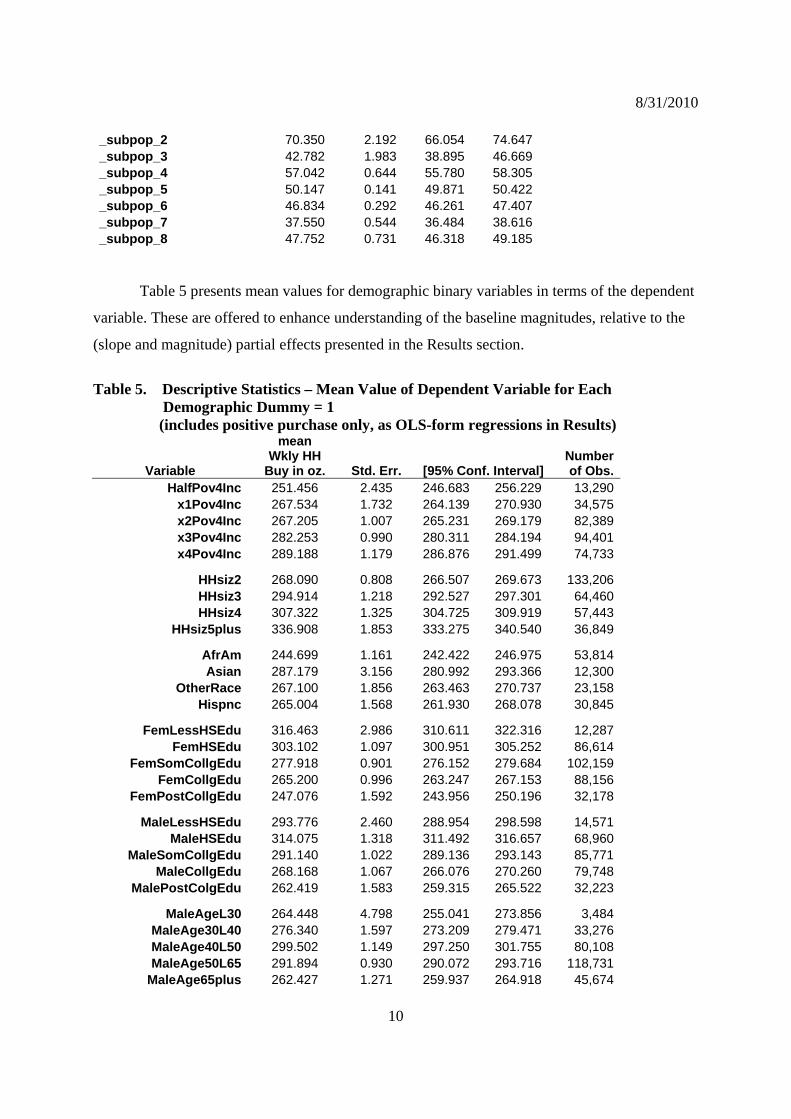
Table 4. Descriptive Statistics – Do Hispanics drink more or less than other Racial groups? mean HHTotOzByPP, over(Hispanic Race) Mean estimation Number of obs = 2003644 Over: Hispanic Race Hisp: 1 = Yes, 2 = No _subpop_1: 1 1 Race: 1 = White _subpop_2: 1 2 2 = Afr Am _subpop_3: 1 3 3 = Asian _subpop_4: 1 4 4 = Other Race _subpop_5: 2 1 White only _subpop_6: 2 2 Afr Am only _subpop_7: 2 3 Asian only _subpop_8: 2 4 Other only

Over Mean Std. Err. [95% Conf. Interval]

HHTotOzByPP _subpop_1 50.037 0.589 48.883 51.192

8/31/2010

10

_subpop_2 70.350 2.192 66.054 74.647_subpop_3 42.782 1.983 38.895 46.669_subpop_4 57.042 0.644 55.780 58.305_subpop_5 50.147 0.141 49.871 50.422_subpop_6 46.834 0.292 46.261 47.407_subpop_7 37.550 0.544 36.484 38.616_subpop_8 47.752 0.731 46.318 49.185

Table 5 presents mean values for demographic binary variables in terms of the dependent

variable. These are offered to enhance understanding of the baseline magnitudes, relative to the

(slope and magnitude) partial effects presented in the Results section.

Table 5. Descriptive Statistics – Mean Value of Dependent Variable for Each Demographic Dummy = 1

(includes positive purchase only, as OLS-form regressions in Results)

Variable

mean Wkly HH

Buy in oz. Std. Err. [95% Conf. Interval] Number of Obs.

HalfPov4Inc 251.456 2.435 246.683 256.229 13,290 x1Pov4Inc 267.534 1.732 264.139 270.930 34,575 x2Pov4Inc 267.205 1.007 265.231 269.179 82,389 x3Pov4Inc 282.253 0.990 280.311 284.194 94,401 x4Pov4Inc 289.188 1.179 286.876 291.499 74,733

HHsiz2 268.090 0.808 266.507 269.673 133,206 HHsiz3 294.914 1.218 292.527 297.301 64,460 HHsiz4 307.322 1.325 304.725 309.919 57,443

HHsiz5plus 336.908 1.853 333.275 340.540 36,849

AfrAm 244.699 1.161 242.422 246.975 53,814 Asian 287.179 3.156 280.992 293.366 12,300

OtherRace 267.100 1.856 263.463 270.737 23,158 Hispnc 265.004 1.568 261.930 268.078 30,845

FemLessHSEdu 316.463 2.986 310.611 322.316 12,287 FemHSEdu 303.102 1.097 300.951 305.252 86,614

FemSomCollgEdu 277.918 0.901 276.152 279.684 102,159 FemCollgEdu 265.200 0.996 263.247 267.153 88,156

FemPostCollgEdu 247.076 1.592 243.956 250.196 32,178

MaleLessHSEdu 293.776 2.460 288.954 298.598 14,571 MaleHSEdu 314.075 1.318 311.492 316.657 68,960

MaleSomCollgEdu 291.140 1.022 289.136 293.143 85,771 MaleCollgEdu 268.168 1.067 266.076 270.260 79,748

MalePostColgEdu 262.419 1.583 259.315 265.522 32,223

MaleAgeL30 264.448 4.798 255.041 273.856 3,484 MaleAge30L40 276.340 1.597 273.209 279.471 33,276 MaleAge40L50 299.502 1.149 297.250 301.755 80,108 MaleAge50L65 291.894 0.930 290.072 293.716 118,731

MaleAge65plus 262.427 1.271 259.937 264.918 45,674

8/31/2010

11

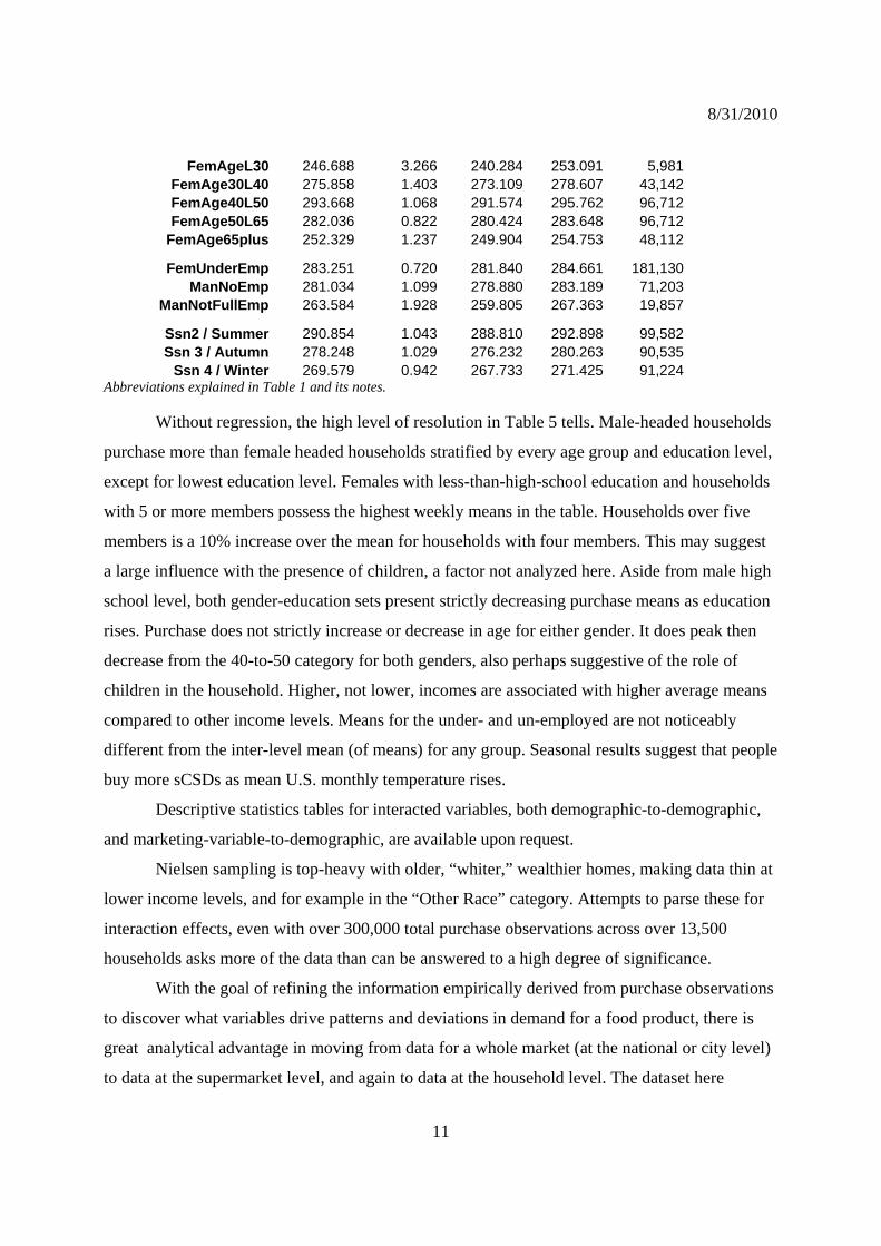
FemAgeL30 246.688 3.266 240.284 253.091 5,981 FemAge30L40 275.858 1.403 273.109 278.607 43,142 FemAge40L50 293.668 1.068 291.574 295.762 96,712 FemAge50L65 282.036 0.822 280.424 283.648 96,712

FemAge65plus 252.329 1.237 249.904 254.753 48,112

FemUnderEmp 283.251 0.720 281.840 284.661 181,130 ManNoEmp 281.034 1.099 278.880 283.189 71,203

ManNotFullEmp 263.584 1.928 259.805 267.363 19,857

Ssn2 / Summer 290.854 1.043 288.810 292.898 99,582 Ssn 3 / Autumn 278.248 1.029 276.232 280.263 90,535

Ssn 4 / Winter 269.579 0.942 267.733 271.425 91,224 Abbreviations explained in Table 1 and its notes.

Without regression, the high level of resolution in Table 5 tells. Male-headed households

purchase more than female headed households stratified by every age group and education level,

except for lowest education level. Females with less-than-high-school education and households

with 5 or more members possess the highest weekly means in the table. Households over five

members is a 10% increase over the mean for households with four members. This may suggest

a large influence with the presence of children, a factor not analyzed here. Aside from male high

school level, both gender-education sets present strictly decreasing purchase means as education

rises. Purchase does not strictly increase or decrease in age for either gender. It does peak then

decrease from the 40-to-50 category for both genders, also perhaps suggestive of the role of

children in the household. Higher, not lower, incomes are associated with higher average means

compared to other income levels. Means for the under- and un-employed are not noticeably

different from the inter-level mean (of means) for any group. Seasonal results suggest that people

buy more sCSDs as mean U.S. monthly temperature rises.

Descriptive statistics tables for interacted variables, both demographic-to-demographic,

and marketing-variable-to-demographic, are available upon request.

Nielsen sampling is top-heavy with older, “whiter,” wealthier homes, making data thin at

lower income levels, and for example in the “Other Race” category. Attempts to parse these for

interaction effects, even with over 300,000 total purchase observations across over 13,500

households asks more of the data than can be answered to a high degree of significance.

With the goal of refining the information empirically derived from purchase observations

to discover what variables drive patterns and deviations in demand for a food product, there is

great analytical advantage in moving from data for a whole market (at the national or city level)

to data at the supermarket level, and again to data at the household level. The dataset here

8/31/2010

12

employed is resolute to the household level, but is still not individual-level data. It is not

possible to identify who in a household or how many in a household are drinking the sCSDs we

observe to be purchased. If one member in a larger household dominates demand for sCSDs,

demand is averaged, despite the individual demand being the true driver, and at consumption

levels above the household average. There is similarly no information about the health, body

mass index, or nutrition education of household members, any of which could prove helpful in

pursuing the question of interest undertaken here.

4. Methodology

In the introduction, I summarized reasons that the regular consumption of sCSDs may not

reflect rational economic behavior from which a utility-based model of demand may be

unambiguously derived. Reduced-form modeling (RFM) offers the implicit advantage of “letting

the data speak for themselves,” without being encumbered by layers of assumptions about

economic behavior and discrete, orderly, quantifiable optimization. RFM also allows for multiple

specifications without violating structural theory or econometric assumptions that can bind

structural models. Multiple specifications may then be employed to explore sequential questions

and to establish proofs of robustness for interpretation of results. This is characteristic of

econometric issues associated with RFM (Gentzkow and Shapiro: 2008; DellaVigna, et. al.:

2009; Dahl and DellaVigna: 2009; Basker: 2005; Chen and Shapiro: 2006).

The large number of zero observations for the dependent variable – total ounces

purchased by a household in one week – highlights that there is a limited dependent variable

(non-negative distribution). The nexus of the research question and the available data defines the

interaction between the dependent variable, the explanatory variables, and the error term being

modeled.

In distinguishing between the extant regression models appropriate for a limited

dependent variable that is continuous and non-negative, one must determine if the data is

censored or truncated. Panel data with continuous information on household purchasers ensures

that there are observations for many explanatory variables even if the dependent variable is not

observed. This defines a censored dependent variable versus a truncated one, truncation

occurring when both dependent and explanatory variables are unobserved above or below a

threshold for a latent explanatory variable. With a censored dependent variable, one must assess

whether the data and research question match existing models, and if so, whether the limitations

8/31/2010

13

associated with any one model are tolerable given the data, research question, and alternative

models.

Given that there is no censoring of negative observations on quantity purchased, is a

linear OLS an acceptable model, once corrected for heteroskedasticy in the error term? Only if

there are no other specification errors that are better addressed by the set of continuous limited

dependent variable models, and indeed OLS results are presented here for baseline comparison.

In his 1979 Econometrica article, James Heckman proposed a model to correct for bias in

the selection of a data sample. There is a sample selection bias problem here, but it is subtle. For

there to be sample selection bias in the selection of households, Nielsen must be contracting

households that do not cumulatively define a representative cross-section of U.S. households.

This conclusion is not supported by the literature (Einav and Leibtag: ).

The research here attempts to distinguish different demographic groups’ responses to

marketing mix variables for sCSDs. A response to marketing variables is involvement in the

specific market in which a decision to purchase or not is made. “Being in” or “selecting into” the

market means at some level a household member actively considers purchase – “the market”

being a solution to an equation consisting not only of sellers, their marketing mix variables, and

buyers, but a venue (the local DMA) that exists distinctly in each period of observation for both

buyers and potential sellers, here one processing period is a week. Thus each observation period

(each week) is counted as a new market in which potential buyers may transact with sellers if

both choose, with the local DMA being the physical space in which transactions may occur.

Modeling household market participation, I code purchase occasion as a 1, and non-

purchase as a 0. The bias of selection into the observation set – the selection bias problem that

modeling must attempt to resolve – becomes clearer as one realizes that a coded non-purchase

“0” represents a household in a metropolitan area in a week, a household that may or may not be

participating in the market. One type of 0 occurs for market participants, who by the definition of

market participant, consider buying, but choose not to buy (e.g., find no lemon-lime flavor, so

buy nothing, or find no discounts this week, so buy nothing). But there is a second type of 0

which occurs for those who never consider buying sCSDs in the observed week: non-participants

in the market. This group’s “0s” reflect their lack of economic presence/being/existence in the

market transaction set of agents-forum-time. Because the 0s are of two types – market

participants with true-zero responses to the current marketing mix, and non-market participants

who are not reacting to the marketing mix in their observed behavior – there is in examining only

8/31/2010

14

the observable 0s, a failure to identify the market participants who choose a no-purchase

response to this period’s marketing mix of variables. Market participation, even for non-purchase

should be coded “1”, when the data presents only a “0.” This is the crux of the sample selection

bias problem – we see only “0s” when we do not see purchase, without knowing whether the

zeros are responses to marketing mix variables by participants in the market, or zeros

characterizing lack of participation in the market.

Econometrically, with yi* as the latent variable for market participation, ix the

explanatory variable set, a vector of coefficients, and an additive error term iu , the attempt is

to model:

iii uxy '* .

To approximate this, we use actual observations yi, and:

yi = 1 when yi* = 1 ,

and yi = 0 when yi* = 0.

But we never observe:

yi = 0 when yi

* = 1.

Observing this would fully identify consideration and rejection of marketing variables, as

opposed to disengagement from the market in a given week. But there is not and will not be data

to comprehensively identify who among our Nielsen households considered purchasing sCSDs

in a sampled week. In other words, the true number of non-purchases that reflect consideration

and rejection of the week’s marketing variables as observable to a potential consumer cannot be

unambiguously distinguished from non-purchases resulting from a household’s complete

inattention to the potentially observable marketing variables for the week.

Because the true rejections of the marketing variables are not observed and entered into

the probit estimation of probability of participation in the market – and if they were this would

expand the number of identified market participation incidents – the probability of participation

is to some unknown amount estimated too low. If we expect that most people who consider

buying a sCSD in fact do, than this deviation may be expected to be low. Regardless of our

expectation, the undercounting of market participation translates into the secondary OLS

estimation and calculation of marginal effects. Those explanatory variables that correlate more

strongly with non-purchase will have slightly deflated coefficients, as a portion of the non-

purchase observations (zeros) correctly belong to a market response set, rather than to the non-

8/31/2010

15

participation set in which they are counted (too many zeros are factored in). Similarly,

explanatory variables that correlate more strongly with purchase will have slightly inflated

coefficients, as some of the non-purchase observations (zeros) correctly belonging to a market

response set, rather than to the non-participation set in which they are counted, will not be

factored in. The magnitude of these effects will be proportional to the extent that the “true-zero

participation responses” exist and are not observed.

The implicit misspecification in modeling the response to the marketing mix defines the

need to discriminate market participants from non-market participants. The Heckman two-step

model establishes two equations, one assessing probability that a household selects into the

market in a given observation period, and the second gauging the outcome of participation. The

dependent variable in the selection equation is a probit probability variable, 1 if purchase

occurred and 0 otherwise. Purchase is equated with market participation, so the dependent

variable does not fully reveal the latent variable of probability of market participation (as distinct

from non-participation, which also generates a 0 observation). “Exclusion restrictions” are

variables that exist only on the probit side of the model, intended to explain selection into the

market without necessarily explaining quantity purchase once committing to purchase.

It is easy to imagine that a highly shelf-stable product like canned or bottled sCSDs may

be stocked in the homes of consumers, and that stock levels may affect likelihood to purchase.

Attempting to construct a household-stock-level variable from recent purchase behavior would

create an autocorrelation problem in OLS regression. As most of my variables of interest are

time-invariant, the standard solutions to this problem (differencing between time periods) is not

appealing. But with the two-equation framework, stocking levels can be entered on the probit

side, and then are regressed only on probability, not on current quantity. As the variable does not

present in both equations, it is not factored into the inverse Mills ratio, which channels

information between the two equations.

Heckman two-step estimation treats the sample selection bias problem as an omitted

variable problem. Because the selection equation is a probit model, it is possible to recover a

standard normal distribution function evaluated at a specific observational value of the

explanatory variable-coefficient matrix, and divide each respective value by the standard error of

the particular normal distribution. This is the denominator of the inverse Mills ratio (IMR), with

numerator being the density of the standard normal distribution function, also evaluated at a

specific observational value of the explanatory variable-coefficient matrix. The IMR is then a

8/31/2010

16

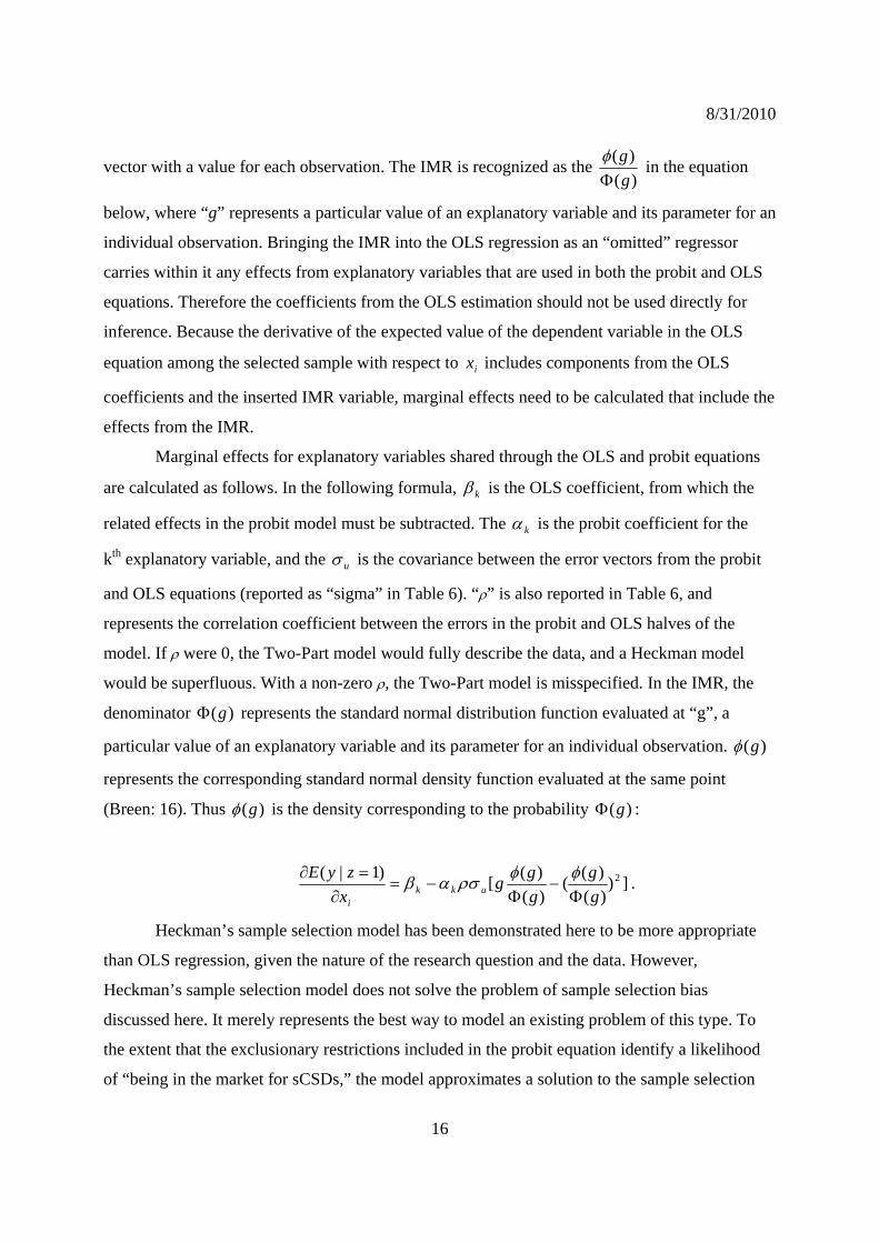
vector with a value for each observation. The IMR is recognized as the )(

)(

g

g

in the equation

below, where “g” represents a particular value of an explanatory variable and its parameter for an

individual observation. Bringing the IMR into the OLS regression as an “omitted” regressor

carries within it any effects from explanatory variables that are used in both the probit and OLS

equations. Therefore the coefficients from the OLS estimation should not be used directly for

inference. Because the derivative of the expected value of the dependent variable in the OLS

equation among the selected sample with respect to ix includes components from the OLS

coefficients and the inserted IMR variable, marginal effects need to be calculated that include the

effects from the IMR.

Marginal effects for explanatory variables shared through the OLS and probit equations

are calculated as follows. In the following formula, k is the OLS coefficient, from which the

related effects in the probit model must be subtracted. The k is the probit coefficient for the

kth explanatory variable, and the u is the covariance between the error vectors from the probit

and OLS equations (reported as “sigma” in Table 6). “” is also reported in Table 6, and

represents the correlation coefficient between the errors in the probit and OLS halves of the

model. If were 0, the Two-Part model would fully describe the data, and a Heckman model

would be superfluous. With a non-zero , the Two-Part model is misspecified. In the IMR, the

denominator )(g represents the standard normal distribution function evaluated at “g”, a

particular value of an explanatory variable and its parameter for an individual observation. )(g

represents the corresponding standard normal density function evaluated at the same point

(Breen: 16). Thus )(g is the density corresponding to the probability )(g :

]))(

)((

)(

)([

)1|( 2

g

g

g

gg

x

zyEukk

i

.

Heckman’s sample selection model has been demonstrated here to be more appropriate

than OLS regression, given the nature of the research question and the data. However,

Heckman’s sample selection model does not solve the problem of sample selection bias

discussed here. It merely represents the best way to model an existing problem of this type. To

the extent that the exclusionary restrictions included in the probit equation identify a likelihood

of “being in the market for sCSDs,” the model approximates a solution to the sample selection

8/31/2010

17

problem, where the OLS, Tobit, or Two-Part models necessarily fail to, and each of these

alternative models would yield biased and inconsistent results to some degree (Breen: 40).

Price promotion/discounting may motivate the decision to purchase, just as it may

motivate quantity of purchase. In the current form, observational data at the household level only

include the existence of a discounted price in a process period only if a purchase was made. As

there is no direct record of discounted price existing when no purchase was made, discounting

variables regressed in the probit equation on selection into the market are perfectly collinear with

purchases, and cannot be included. At a later stage of this research, the existence of discounted

price may be recovered from other household’s purchases within the DMA for that process

period.

5. Results

All coefficients (except those interacted with the advertising mix and the exclusionary

restrictions in the probit equation) may be interpreted as the rate of change in household-total-

ounces-purchased-in-a-week (the dependent variable “HHTotOzByPP”), due to a one-unit

change in value of the explanatory variable. For all of the demographic variables, season

variables, and the marketing variable “Sale,” this is for a binary-value change from 0 to 1. For

the price index, this unit change is in dollars per ounce. Coefficients on advertising mix and the

exclusionary restrictions in the probit equation may be interpreted only to sign and significance,

not magnitude in any meaningful unit.

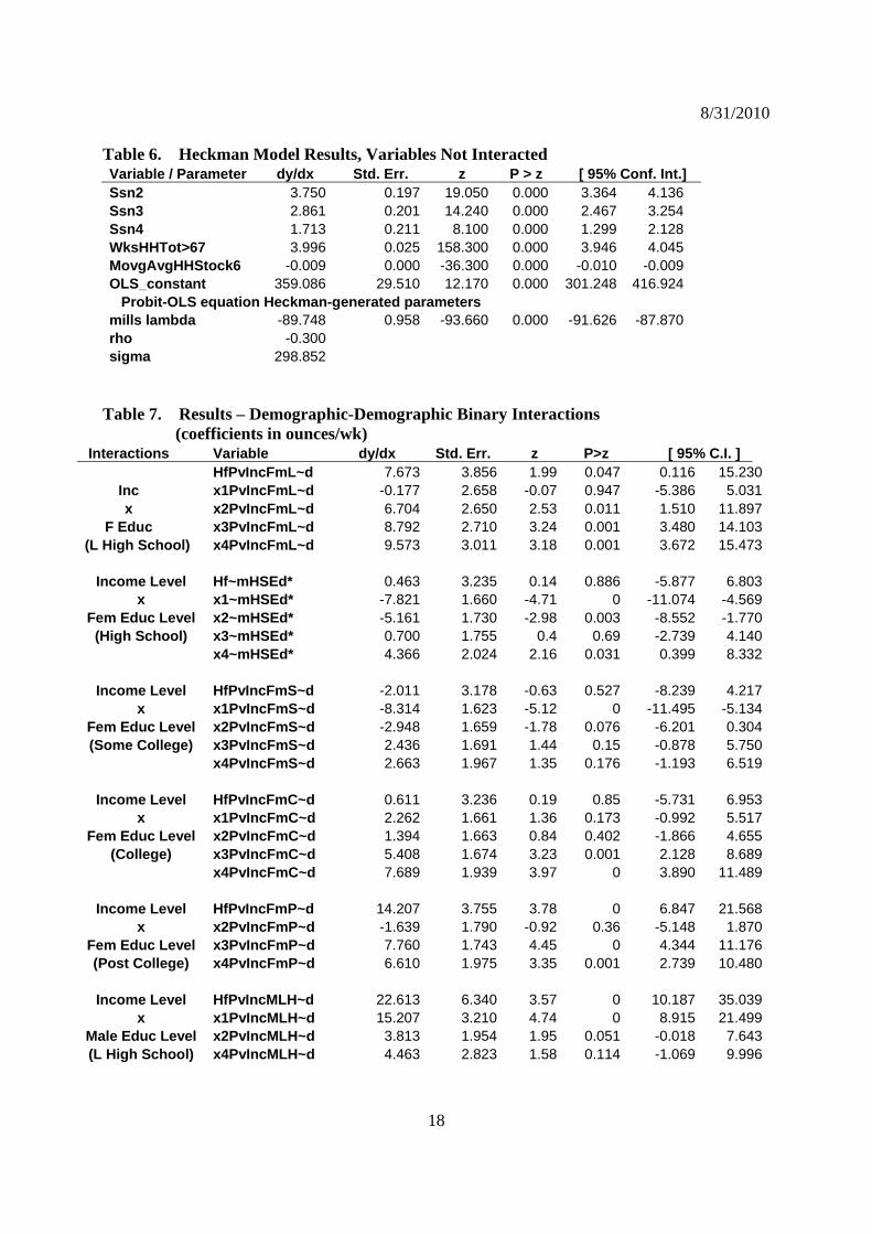
Table 6 shows that relevant coefficients (i.e., on all un-interacted variables) are of the

expected sign and significant to p-values of zero to at least the fourth decimal place. Seasons

(Spring is control) are of expected relative magnitudes, largest in Summer, followed by Fall,

with Winter last (but still greater than Spring). The exclusion restriction variables that are

intended to define market participation are of expected sign (interpretation of magnitudes or in

ounces does not apply), meaning that higher estimated household stocks of sCSDs in a given

week do diminish likelihood of purchase in that week; and the more often in a year that

households buy at least two liters of sCSDs during any week, the higher is their general

probability of market participation as measured in the Heckman model applied here. The non-

zero correlation coefficient between the Probit and OLS sides of the Heckman (=-0.3) rules out

the Two-Part model specification.

8/31/2010

18

Table 6. Heckman Model Results, Variables Not Interacted Variable / Parameter dy/dx Std. Err. z P > z [ 95% Conf. Int.] Ssn2 3.750 0.197 19.050 0.000 3.364 4.136 Ssn3 2.861 0.201 14.240 0.000 2.467 3.254 Ssn4 1.713 0.211 8.100 0.000 1.299 2.128 WksHHTot>67 3.996 0.025 158.300 0.000 3.946 4.045 MovgAvgHHStock6 -0.009 0.000 -36.300 0.000 -0.010 -0.009 OLS_constant 359.086 29.510 12.170 0.000 301.248 416.924 Probit-OLS equation Heckman-generated parameters mills lambda -89.748 0.958 -93.660 0.000 -91.626 -87.870 rho -0.300 sigma 298.852

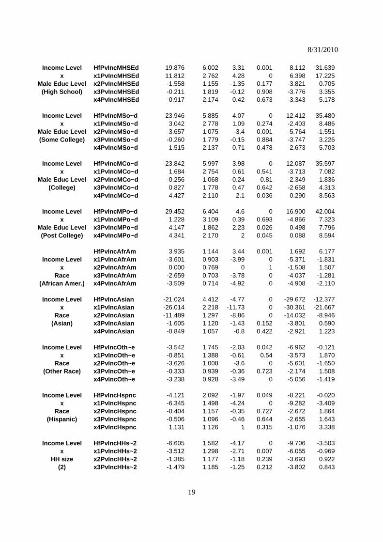
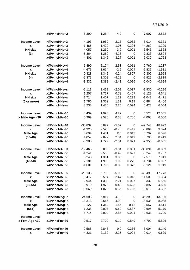
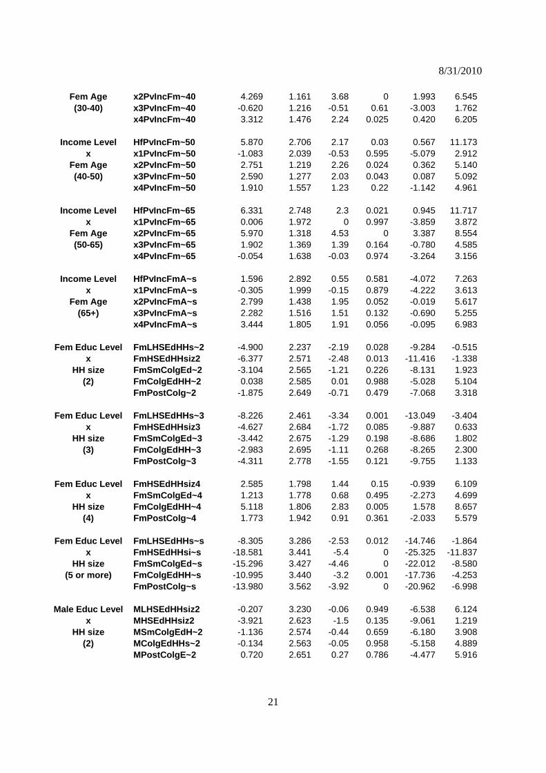
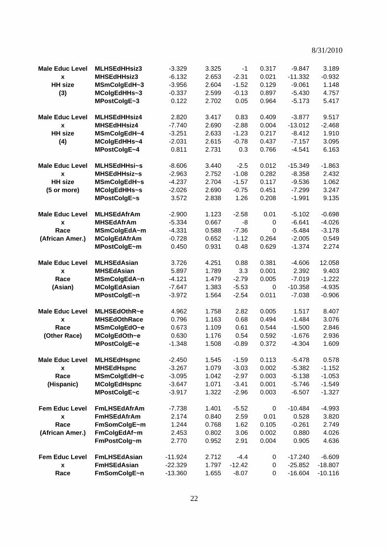
Table 7. Results – Demographic-Demographic Binary Interactions

(coefficients in ounces/wk) Interactions Variable dy/dx Std. Err. z P>z [ 95% C.I. ]

HfPvIncFmL~d 7.673 3.856 1.99 0.047 0.116 15.230Inc x1PvIncFmL~d -0.177 2.658 -0.07 0.947 -5.386 5.031x x2PvIncFmL~d 6.704 2.650 2.53 0.011 1.510 11.897

F Educ x3PvIncFmL~d 8.792 2.710 3.24 0.001 3.480 14.103(L High School) x4PvIncFmL~d 9.573 3.011 3.18 0.001 3.672 15.473

Income Level Hf~mHSEd* 0.463 3.235 0.14 0.886 -5.877 6.803x x1~mHSEd* -7.821 1.660 -4.71 0 -11.074 -4.569

Fem Educ Level x2~mHSEd* -5.161 1.730 -2.98 0.003 -8.552 -1.770(High School) x3~mHSEd* 0.700 1.755 0.4 0.69 -2.739 4.140

x4~mHSEd* 4.366 2.024 2.16 0.031 0.399 8.332

Income Level HfPvIncFmS~d -2.011 3.178 -0.63 0.527 -8.239 4.217x x1PvIncFmS~d -8.314 1.623 -5.12 0 -11.495 -5.134

Fem Educ Level x2PvIncFmS~d -2.948 1.659 -1.78 0.076 -6.201 0.304(Some College) x3PvIncFmS~d 2.436 1.691 1.44 0.15 -0.878 5.750

x4PvIncFmS~d 2.663 1.967 1.35 0.176 -1.193 6.519

Income Level HfPvIncFmC~d 0.611 3.236 0.19 0.85 -5.731 6.953x x1PvIncFmC~d 2.262 1.661 1.36 0.173 -0.992 5.517

Fem Educ Level x2PvIncFmC~d 1.394 1.663 0.84 0.402 -1.866 4.655(College) x3PvIncFmC~d 5.408 1.674 3.23 0.001 2.128 8.689

x4PvIncFmC~d 7.689 1.939 3.97 0 3.890 11.489

Income Level HfPvIncFmP~d 14.207 3.755 3.78 0 6.847 21.568x x2PvIncFmP~d -1.639 1.790 -0.92 0.36 -5.148 1.870

Fem Educ Level x3PvIncFmP~d 7.760 1.743 4.45 0 4.344 11.176(Post College) x4PvIncFmP~d 6.610 1.975 3.35 0.001 2.739 10.480

Income Level HfPvIncMLH~d 22.613 6.340 3.57 0 10.187 35.039

x x1PvIncMLH~d 15.207 3.210 4.74 0 8.915 21.499Male Educ Level x2PvIncMLH~d 3.813 1.954 1.95 0.051 -0.018 7.643(L High School) x4PvIncMLH~d 4.463 2.823 1.58 0.114 -1.069 9.996

8/31/2010

19

Income Level HfPvIncMHSEd 19.876 6.002 3.31 0.001 8.112 31.639x x1PvIncMHSEd 11.812 2.762 4.28 0 6.398 17.225

Male Educ Level x2PvIncMHSEd -1.558 1.155 -1.35 0.177 -3.821 0.705(High School) x3PvIncMHSEd -0.211 1.819 -0.12 0.908 -3.776 3.355

x4PvIncMHSEd 0.917 2.174 0.42 0.673 -3.343 5.178

Income Level HfPvIncMSo~d 23.946 5.885 4.07 0 12.412 35.480x x1PvIncMSo~d 3.042 2.778 1.09 0.274 -2.403 8.486

Male Educ Level x2PvIncMSo~d -3.657 1.075 -3.4 0.001 -5.764 -1.551(Some College) x3PvIncMSo~d -0.260 1.779 -0.15 0.884 -3.747 3.226

x4PvIncMSo~d 1.515 2.137 0.71 0.478 -2.673 5.703

Income Level HfPvIncMCo~d 23.842 5.997 3.98 0 12.087 35.597x x1PvIncMCo~d 1.684 2.754 0.61 0.541 -3.713 7.082

Male Educ Level x2PvIncMCo~d -0.256 1.068 -0.24 0.81 -2.349 1.836(College) x3PvIncMCo~d 0.827 1.778 0.47 0.642 -2.658 4.313

x4PvIncMCo~d 4.427 2.110 2.1 0.036 0.290 8.563

Income Level HfPvIncMPo~d 29.452 6.404 4.6 0 16.900 42.004x x1PvIncMPo~d 1.228 3.109 0.39 0.693 -4.866 7.323

Male Educ Level x3PvIncMPo~d 4.147 1.862 2.23 0.026 0.498 7.796(Post College) x4PvIncMPo~d 4.341 2.170 2 0.045 0.088 8.594

HfPvIncAfrAm 3.935 1.144 3.44 0.001 1.692 6.177

Income Level x1PvIncAfrAm -3.601 0.903 -3.99 0 -5.371 -1.831x x2PvIncAfrAm 0.000 0.769 0 1 -1.508 1.507

Race x3PvIncAfrAm -2.659 0.703 -3.78 0 -4.037 -1.281(African Amer.) x4PvIncAfrAm -3.509 0.714 -4.92 0 -4.908 -2.110

Income Level HfPvIncAsian -21.024 4.412 -4.77 0 -29.672 -12.377

x x1PvIncAsian -26.014 2.218 -11.73 0 -30.361 -21.667Race x2PvIncAsian -11.489 1.297 -8.86 0 -14.032 -8.946

(Asian) x3PvIncAsian -1.605 1.120 -1.43 0.152 -3.801 0.590 x4PvIncAsian -0.849 1.057 -0.8 0.422 -2.921 1.223

Income Level HfPvIncOth~e -3.542 1.745 -2.03 0.042 -6.962 -0.121x x1PvIncOth~e -0.851 1.388 -0.61 0.54 -3.573 1.870

Race x2PvIncOth~e -3.626 1.008 -3.6 0 -5.601 -1.650(Other Race) x3PvIncOth~e -0.333 0.939 -0.36 0.723 -2.174 1.508

x4PvIncOth~e -3.238 0.928 -3.49 0 -5.056 -1.419

Income Level HfPvIncHspnc -4.121 2.092 -1.97 0.049 -8.221 -0.020x x1PvIncHspnc -6.345 1.498 -4.24 0 -9.282 -3.409

Race x2PvIncHspnc -0.404 1.157 -0.35 0.727 -2.672 1.864(Hispanic) x3PvIncHspnc -0.506 1.096 -0.46 0.644 -2.655 1.643

x4PvIncHspnc 1.131 1.126 1 0.315 -1.076 3.338

Income Level HfPvIncHHs~2 -6.605 1.582 -4.17 0 -9.706 -3.503x x1PvIncHHs~2 -3.512 1.298 -2.71 0.007 -6.055 -0.969

HH size x2PvIncHHs~2 -1.385 1.177 -1.18 0.239 -3.693 0.922(2) x3PvIncHHs~2 -1.479 1.185 -1.25 0.212 -3.802 0.843

8/31/2010

20

x4PvIncHHs~2 -5.390 1.284 -4.2 0 -7.907 -2.872

Income Level HfPvIncHHs~3 -4.193 1.950 -2.15 0.032 -8.014 -0.371x x1PvIncHHs~3 -1.485 1.420 -1.05 0.296 -4.269 1.299

HH size x2PvIncHHs~3 -4.057 1.269 -3.2 0.001 -6.545 -1.568(3) x3PvIncHHs~3 -5.364 1.260 -4.26 0 -7.833 -2.894

x4PvIncHHs~3 -4.401 1.346 -3.27 0.001 -7.039 -1.763

Income Level HfPvIncHHs~4 -5.499 2.174 -2.53 0.011 -9.760 -1.237x x1PvIncHHs~4 -4.675 1.614 -2.9 0.004 -7.839 -1.511

HH size x2PvIncHHs~4 0.328 1.342 0.24 0.807 -2.302 2.958(4) x3PvIncHHs~4 -5.373 1.303 -4.12 0 -7.927 -2.819

x4PvIncHHs~4 -3.332 1.382 -2.41 0.016 -6.040 -0.624

Income Level HfPvIncHHs~s -5.113 2.458 -2.08 0.037 -9.930 -0.296x x1PvIncHHs~s 1.257 1.727 0.73 0.467 -2.127 4.641

HH size x2PvIncHHs~s 1.714 1.407 1.22 0.223 -1.043 4.471(5 or more) x3PvIncHHs~s 1.786 1.362 1.31 0.19 -0.884 4.456

x4PvIncHHs~s 3.238 1.436 2.25 0.024 0.423 6.054

Income Level x2PvIncMA~30 8.439 1.998 4.22 0 4.523 12.355x Male Age <30 x3PvIncMA~30 0.969 2.570 0.38 0.706 -4.068 6.006

Income Level HfPvIncMA~40 -30.832 6.077 -5.07 0 -42.743 -18.922

x x1PvIncMA~40 -1.920 2.523 -0.76 0.447 -6.864 3.024Male Age x2PvIncMA~40 3.694 1.481 2.5 0.013 0.792 6.596

(30-40) x3PvIncMA~40 4.857 2.072 2.34 0.019 0.796 8.919 x4PvIncMA~40 -3.980 1.722 -2.31 0.021 -7.356 -0.605

Income Level HfPvIncMA~50 -19.465 5.830 -3.34 0.001 -30.891 -8.039x x1PvIncMA~50 -1.241 2.555 -0.49 0.627 -6.249 3.767

Male Age x2PvIncMA~50 5.243 1.361 3.85 0 2.575 7.911(40-50) x3PvIncMA~50 2.181 1.998 1.09 0.275 -1.734 6.097

x4PvIncMA~50 -1.601 1.796 -0.89 0.373 -5.121 1.919

Income Level HfPvIncMA~65 -29.136 5.798 -5.03 0 -40.499 -17.773x x1PvIncMA~65 -6.417 2.594 -2.47 0.013 -11.500 -1.334

Male Age x2PvIncMA~65 2.944 1.332 2.21 0.027 0.332 5.555(50-65) x3PvIncMA~65 0.970 1.973 0.49 0.623 -2.897 4.836

x4PvIncMA~65 0.660 1.873 0.35 0.725 -3.012 4.332

Income Level HfPvIncMAg~s -24.698 5.914 -4.18 0 -36.290 -13.106x x1PvIncMAg~s -13.313 2.666 -4.99 0 -18.538 -8.088

Male Age x2PvIncMAg~s 2.127 1.369 1.55 0.12 -0.557 4.811(65+) x3PvIncMAg~s 1.238 2.007 0.62 0.537 -2.695 5.170

x4PvIncMAg~s -5.714 2.002 -2.85 0.004 -9.638 -1.790Income Level

x Fem Age <30 x1PvIncFm~30 0.517 2.709 0.19 0.849 -4.792 5.826

Income Level HfPvIncFm~40 2.568 2.843 0.9 0.366 -3.004 8.140x x1PvIncFm~40 -4.821 2.139 -2.25 0.024 -9.014 -0.629

8/31/2010

21

Fem Age x2PvIncFm~40 4.269 1.161 3.68 0 1.993 6.545(30-40) x3PvIncFm~40 -0.620 1.216 -0.51 0.61 -3.003 1.762

x4PvIncFm~40 3.312 1.476 2.24 0.025 0.420 6.205

Income Level HfPvIncFm~50 5.870 2.706 2.17 0.03 0.567 11.173x x1PvIncFm~50 -1.083 2.039 -0.53 0.595 -5.079 2.912

Fem Age x2PvIncFm~50 2.751 1.219 2.26 0.024 0.362 5.140(40-50) x3PvIncFm~50 2.590 1.277 2.03 0.043 0.087 5.092

x4PvIncFm~50 1.910 1.557 1.23 0.22 -1.142 4.961

Income Level HfPvIncFm~65 6.331 2.748 2.3 0.021 0.945 11.717x x1PvIncFm~65 0.006 1.972 0 0.997 -3.859 3.872

Fem Age x2PvIncFm~65 5.970 1.318 4.53 0 3.387 8.554(50-65) x3PvIncFm~65 1.902 1.369 1.39 0.164 -0.780 4.585

x4PvIncFm~65 -0.054 1.638 -0.03 0.974 -3.264 3.156

Income Level HfPvIncFmA~s 1.596 2.892 0.55 0.581 -4.072 7.263x x1PvIncFmA~s -0.305 1.999 -0.15 0.879 -4.222 3.613

Fem Age x2PvIncFmA~s 2.799 1.438 1.95 0.052 -0.019 5.617(65+) x3PvIncFmA~s 2.282 1.516 1.51 0.132 -0.690 5.255

x4PvIncFmA~s 3.444 1.805 1.91 0.056 -0.095 6.983

Fem Educ Level FmLHSEdHHs~2 -4.900 2.237 -2.19 0.028 -9.284 -0.515x FmHSEdHHsiz2 -6.377 2.571 -2.48 0.013 -11.416 -1.338

HH size FmSmColgEd~2 -3.104 2.565 -1.21 0.226 -8.131 1.923(2) FmColgEdHH~2 0.038 2.585 0.01 0.988 -5.028 5.104

FmPostColg~2 -1.875 2.649 -0.71 0.479 -7.068 3.318

Fem Educ Level FmLHSEdHHs~3 -8.226 2.461 -3.34 0.001 -13.049 -3.404x FmHSEdHHsiz3 -4.627 2.684 -1.72 0.085 -9.887 0.633

HH size FmSmColgEd~3 -3.442 2.675 -1.29 0.198 -8.686 1.802(3) FmColgEdHH~3 -2.983 2.695 -1.11 0.268 -8.265 2.300

FmPostColg~3 -4.311 2.778 -1.55 0.121 -9.755 1.133

Fem Educ Level FmHSEdHHsiz4 2.585 1.798 1.44 0.15 -0.939 6.109x FmSmColgEd~4 1.213 1.778 0.68 0.495 -2.273 4.699

HH size FmColgEdHH~4 5.118 1.806 2.83 0.005 1.578 8.657(4) FmPostColg~4 1.773 1.942 0.91 0.361 -2.033 5.579

Fem Educ Level FmLHSEdHHs~s -8.305 3.286 -2.53 0.012 -14.746 -1.864

x FmHSEdHHsi~s -18.581 3.441 -5.4 0 -25.325 -11.837HH size FmSmColgEd~s -15.296 3.427 -4.46 0 -22.012 -8.580

(5 or more) FmColgEdHH~s -10.995 3.440 -3.2 0.001 -17.736 -4.253 FmPostColg~s -13.980 3.562 -3.92 0 -20.962 -6.998

Male Educ Level MLHSEdHHsiz2 -0.207 3.230 -0.06 0.949 -6.538 6.124x MHSEdHHsiz2 -3.921 2.623 -1.5 0.135 -9.061 1.219

HH size MSmColgEdH~2 -1.136 2.574 -0.44 0.659 -6.180 3.908(2) MColgEdHHs~2 -0.134 2.563 -0.05 0.958 -5.158 4.889

MPostColgE~2 0.720 2.651 0.27 0.786 -4.477 5.916

8/31/2010

22

Male Educ Level MLHSEdHHsiz3 -3.329 3.325 -1 0.317 -9.847 3.189x MHSEdHHsiz3 -6.132 2.653 -2.31 0.021 -11.332 -0.932

HH size MSmColgEdH~3 -3.956 2.604 -1.52 0.129 -9.061 1.148(3) MColgEdHHs~3 -0.337 2.599 -0.13 0.897 -5.430 4.757

MPostColgE~3 0.122 2.702 0.05 0.964 -5.173 5.417

Male Educ Level MLHSEdHHsiz4 2.820 3.417 0.83 0.409 -3.877 9.517x MHSEdHHsiz4 -7.740 2.690 -2.88 0.004 -13.012 -2.468

HH size MSmColgEdH~4 -3.251 2.633 -1.23 0.217 -8.412 1.910(4) MColgEdHHs~4 -2.031 2.615 -0.78 0.437 -7.157 3.095

MPostColgE~4 0.811 2.731 0.3 0.766 -4.541 6.163

Male Educ Level MLHSEdHHsi~s -8.606 3.440 -2.5 0.012 -15.349 -1.863x MHSEdHHsiz~s -2.963 2.752 -1.08 0.282 -8.358 2.432

HH size MSmColgEdH~s -4.237 2.704 -1.57 0.117 -9.536 1.062(5 or more) MColgEdHHs~s -2.026 2.690 -0.75 0.451 -7.299 3.247

MPostColgE~s 3.572 2.838 1.26 0.208 -1.991 9.135

Male Educ Level MLHSEdAfrAm -2.900 1.123 -2.58 0.01 -5.102 -0.698x MHSEdAfrAm -5.334 0.667 -8 0 -6.641 -4.026

Race MSmColgEdA~m -4.331 0.588 -7.36 0 -5.484 -3.178(African Amer.) MColgEdAfrAm -0.728 0.652 -1.12 0.264 -2.005 0.549

MPostColgE~m 0.450 0.931 0.48 0.629 -1.374 2.274

Male Educ Level MLHSEdAsian 3.726 4.251 0.88 0.381 -4.606 12.058x MHSEdAsian 5.897 1.789 3.3 0.001 2.392 9.403

Race MSmColgEdA~n -4.121 1.479 -2.79 0.005 -7.019 -1.222(Asian) MColgEdAsian -7.647 1.383 -5.53 0 -10.358 -4.935

MPostColgE~n -3.972 1.564 -2.54 0.011 -7.038 -0.906

Male Educ Level MLHSEdOthR~e 4.962 1.758 2.82 0.005 1.517 8.407x MHSEdOthRace 0.796 1.163 0.68 0.494 -1.484 3.076

Race MSmColgEdO~e 0.673 1.109 0.61 0.544 -1.500 2.846(Other Race) MColgEdOth~e 0.630 1.176 0.54 0.592 -1.676 2.936

MPostColgE~e -1.348 1.508 -0.89 0.372 -4.304 1.609

Male Educ Level MLHSEdHspnc -2.450 1.545 -1.59 0.113 -5.478 0.578x MHSEdHspnc -3.267 1.079 -3.03 0.002 -5.382 -1.152

Race MSmColgEdH~c -3.095 1.042 -2.97 0.003 -5.138 -1.053(Hispanic) MColgEdHspnc -3.647 1.071 -3.41 0.001 -5.746 -1.549

MPostColgE~c -3.917 1.322 -2.96 0.003 -6.507 -1.327

Fem Educ Level FmLHSEdAfrAm -7.738 1.401 -5.52 0 -10.484 -4.993x FmHSEdAfrAm 2.174 0.840 2.59 0.01 0.528 3.820

Race FmSomColgE~m 1.244 0.768 1.62 0.105 -0.261 2.749(African Amer.) FmColgEdAf~m 2.453 0.802 3.06 0.002 0.880 4.026

FmPostColg~m 2.770 0.952 2.91 0.004 0.905 4.636

Fem Educ Level FmLHSEdAsian -11.924 2.712 -4.4 0 -17.240 -6.609x FmHSEdAsian -22.329 1.797 -12.42 0 -25.852 -18.807

Race FmSomColgE~n -13.360 1.655 -8.07 0 -16.604 -10.116

8/31/2010

23

(Asian) FmColgEdAs~n -13.117 1.519 -8.63 0 -16.094 -10.139 FmPostColg~n -11.112 1.745 -6.37 0 -14.531 -7.692

Fem Educ Level FmLHSEdOth~e 6.149 1.787 3.44 0.001 2.647 9.651x FmHSEdOthR~e -0.832 1.326 -0.63 0.53 -3.430 1.766

Race FmSomColgE~e -2.385 1.238 -1.93 0.054 -4.811 0.041(Other Race) FmColgEdOt~e -5.478 1.263 -4.34 0 -7.955 -3.002

FmPostColg~e -0.209 1.687 -0.12 0.901 -3.514 3.097

Fem Educ Level FmLHSEdHspnc -7.033 1.671 -4.21 0 -10.308 -3.759x FmHSEdHspnc 0.252 1.295 0.19 0.846 -2.287 2.790

Race FmSomColgE~c 0.308 1.258 0.24 0.807 -2.157 2.773(Hispanic) FmColgEdHs~c 4.135 1.294 3.2 0.001 1.599 6.672

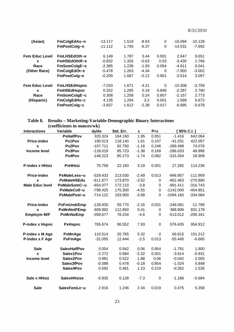
FmPostColg~c -3.837 1.612 -2.38 0.017 -6.995 -0.678 Table 8. Results – Marketing-Variable-Demographic Binary Interactions (coefficients in ounces/wk)

Interactions Variable dy/dx Std. Err. z P>z [ 95% C.I. ] PxHalfPov 320.324 164.160 1.95 0.051 -1.416 642.064

Price-index Px1Pov 190.513 118.140 1.61 0.107 -41.031 422.057x Px2Pov -107.711 92.750 -1.16 0.246 -289.498 74.076

Income level Px3Pov -118.019 85.723 -1.38 0.169 -286.033 49.996 Px4Pov -148.223 85.273 -1.74 0.082 -315.354 18.908

P-index x HHsiz PxHHsiz 70.759 22.183 3.19 0.001 27.282 114.236

Price-index PxMaleLess~u -529.433 213.030 -2.49 0.013 -946.957 -111.909x PxMaleHSEdu -611.677 173.870 -3.52 0 -952.463 -270.890

Male Educ level PxMaleSomC~u -654.077 172.110 -3.8 0 -991.411 -316.743 PxMaleColl~u -798.425 175.300 -4.55 0 -1142.000 -454.851 PxMalePost~u -714.122 193.900 -3.68 0 -1094.160 -334.084

Price-index PxFmUndrEmp -128.935 59.770 -2.16 0.031 -246.081 -11.789x PxMnNotFEmp 609.992 112.850 5.41 0 388.806 831.178

Employm M/F PxMnNoEmp -359.677 78.234 -4.6 0 -513.012 -206.341

P-index x Hspnc PxHspnc 765.674 96.552 7.93 0 576.435 954.912

P-index x M Age PxMnAge 110.514 20.765 5.32 0 69.815 151.212P-index x F Age PxFmAge -31.055 12.444 -2.5 0.013 -55.445 -6.665

Sale SalexHalfPov 0.054 0.942 0.06 0.954 -1.791 1.900

x Salex1Pov -2.272 0.684 -3.32 0.001 -3.614 -0.931Income level Salex2Pov 0.981 0.522 1.88 0.06 -0.042 2.005

Salex3fPov -0.088 0.478 -0.18 0.854 -1.024 0.848 Salex4Pov 0.592 0.481 1.23 0.219 -0.352 1.535

Sale x HHsiz SalexHHsize -0.935 0.128 -7.3 0 -1.186 -0.684

Sale SalexFemLe~u 2.916 1.246 2.34 0.019 0.475 5.358

8/31/2010

24

x SalexFemHS~u 5.545 0.983 5.64 0 3.619 7.472Fem Educ level SalexFemSo~u 5.182 0.964 5.38 0 3.293 7.071

SalexFemCo~u 2.752 0.955 2.88 0.004 0.880 4.624 SalexFemPCo~u 3.793 1.044 3.63 0 1.747 5.839

Sale SalexFmUnd~p -0.263 0.334 -0.79 0.431 -0.918 0.392x SalexMnNot~p -2.674 0.670 -3.99 0 -3.988 -1.360

Employm M/F SalexMnNoEmp -0.430 0.454 -0.95 0.344 -1.320 0.461

Sale SalexAfrAm 2.801 0.428 6.55 0 1.962 3.640x SalexAsian 6.167 0.794 7.77 0 4.611 7.723

Race SalexOthrRac 1.451 0.730 1.99 0.047 0.020 2.883 SalexHspnc -2.590 0.645 -4.02 0 -3.853 -1.326

Sale x Age (M) SalexMnAge 0.244 0.062 3.94 0 0.123 0.366Sale x Age (F) SalexFmAge 0.283 0.101 2.8 0.005 0.085 0.481

Advertsg x HHsiz AdvxHH~z 0.002 0.000 5.54 0 0.001 0.003

advertising interactions not in ounces Advertsng AdvxAf~m 0.003 0.002 1.88 0.06 0.000 0.006

x AdvxAs~n 0.005 0.003 1.77 0.077 -0.001 0.011Race AdvxOt~c 0.004 0.003 1.75 0.081 -0.001 0.009

AdvxHs~c -0.007 0.002 -3.39 0.001 -0.012 -0.003

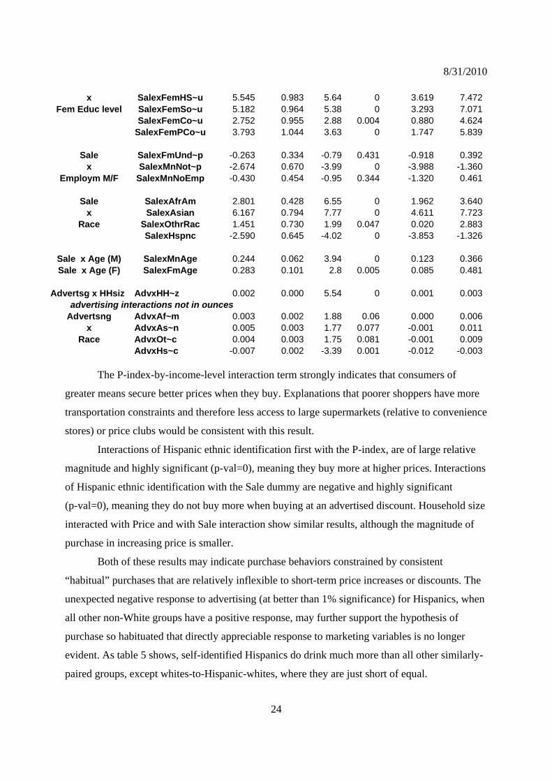
The P-index-by-income-level interaction term strongly indicates that consumers of

greater means secure better prices when they buy. Explanations that poorer shoppers have more

transportation constraints and therefore less access to large supermarkets (relative to convenience

stores) or price clubs would be consistent with this result.

Interactions of Hispanic ethnic identification first with the P-index, are of large relative

magnitude and highly significant (p-val=0), meaning they buy more at higher prices. Interactions

of Hispanic ethnic identification with the Sale dummy are negative and highly significant

(p-val=0), meaning they do not buy more when buying at an advertised discount. Household size

interacted with Price and with Sale interaction show similar results, although the magnitude of

purchase in increasing price is smaller.

Both of these results may indicate purchase behaviors constrained by consistent

“habitual” purchases that are relatively inflexible to short-term price increases or discounts. The

unexpected negative response to advertising (at better than 1% significance) for Hispanics, when

all other non-White groups have a positive response, may further support the hypothesis of

purchase so habituated that directly appreciable response to marketing variables is no longer

evident. As table 5 shows, self-identified Hispanics do drink much more than all other similarly-

paired groups, except whites-to-Hispanic-whites, where they are just short of equal.

8/31/2010

25

The interaction of P-index-by-Male-Head-of-Household-Education-level shows a strong

negative quantity response to a rising price. This response strengthens as education level rises,

but peaks at college education. These effects are all significant at 1.5% or better, and are

consistent with the belief that men respond directly to price as a marketing variable. An inference

that the need to respond to price incentives may taper off with the extra income afforded by post-

graduate education would be consistent with these results. P-index-by-Female-Head-of-

Household-Education-level were mixed and poor performers by statistical significance in

previous specifications, and were dropped from this model (as were the interactions of Male

Education levels with the Sale dummy). In contrast, the Sale-by-Female-Head-of-Household-

Education-level interactions demonstrate that women at all education levels respond positively to

price promotions (all at better than a 2% significance level) – discounting being female’s

marketing variable of choice, versus the male’s price variable.

Marginal effects are often negative when interacting with the lowest income level, but

there is a noticeable break from this in the interaction of female education and income level.

There is evidence that the rising income effect dominates the offsetting effect of rising education

as incomes move into the upper levels. This balances against other results that suggest that

formal education level may proxy for a level of nutrition awareness that would eschew sCSD

purchase.

Marginal analysis supports with constrained consistency an argument that sCSDs act as a

luxury good (whose demand rises with income), but only for income rises moving out of poverty

range, and again at higher incomes. In between, however, the quantity of sCSDs drops with

rising income.

Previous specifications suggested that there is not enough variability in the DMA-level

advertising data used in this specification to ask for higher resolution through interactions. All

coefficients failed to be statistically different from zero when the advertising variable was as

heavily interacted with demographic levels as Price and Sale are in this specification. This is the

reason that advertising interaction was restricted to the HHsize categorical variable and Race

groups only. The gains in statistical significance are obvious, with all of these five significant

below the 10 % level.

8/31/2010

26

5.1 naïve OLS performance versus the econometric selection model specification

As specified, most interactive variable coefficients are interpretable in ounces per week

when they are statistically significant to an acceptable chosen level. Thus the magnitudes of the

variables in relation to each other become informative to a degree that is no longer possible when

the statistical effect approaches zero, and inference is restricted to just the sign of the variable.

The OLS results were rarely significant and will only be partially included here because the

argument can be effectively made using less paper. Table 9 demonstrates that the sample

selection model strongly outperformed the OLS estimation by a simple count of interacted

variables of interest significant at the 10% level or better.

Table 9. Comparison of OLS and Heckman Results – Incidence of Statistical Significance Across Interacted Variable Sets

Interaction Type OLS HeckmanDemographic- Demographic # Out of 220 6 132 Demographic - Demographic % Out of 220 3% 60% Marketing- Demographic # Out of 42 10 35 Marketing- Demographic %Out of 42 24% 83%

OLS coefficients were routinely an order of magnitude higher than Heckman coefficients

(that had been adjusted down using the marginal effects correction necessary for proper

inference). The differences between variables, once adjusting for magnitude differences across

the two models, seemed to track in roughly similar patterns, but only for certain blocks of

interactions. The pattern of statistically insignificant variables across the level groups made

statistically meaningful inference from OLS results unreliable at best, and intractable at worst.

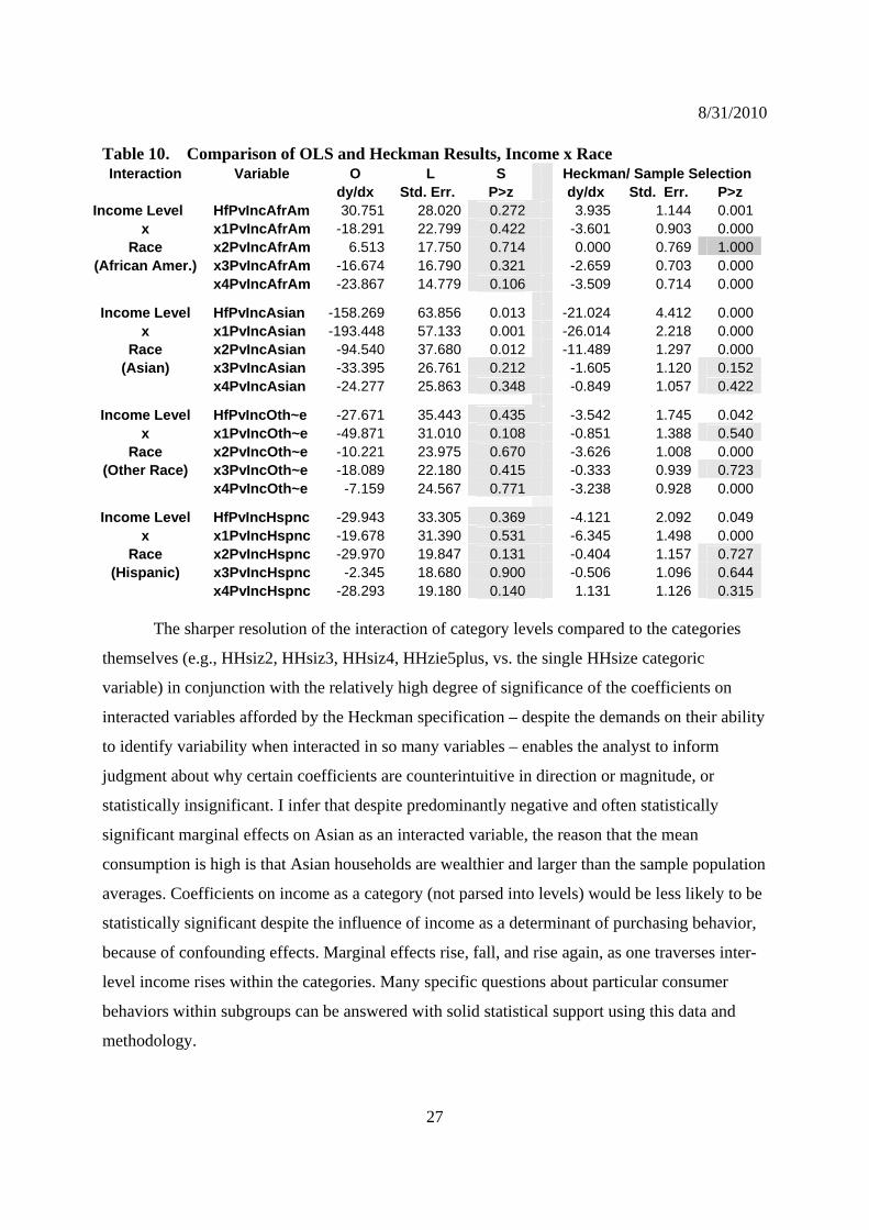
Table 10 presents the interaction block of level comparisons most statistically significant in the

OLS estimation (the only one of its kind), against the same block of results from the Heckman.

Both results are for the OLS equation on only positive purchases. Confidence intervals and z

scores have been dropped to accommodate page width.

8/31/2010

27

Table 10. Comparison of OLS and Heckman Results, Income x Race Interaction Variable O L S Heckman/ Sample Selection

dy/dx Std. Err. P>z dy/dx Std. Err. P>z Income Level HfPvIncAfrAm 30.751 28.020 0.272 3.935 1.144 0.001

x x1PvIncAfrAm -18.291 22.799 0.422 -3.601 0.903 0.000Race x2PvIncAfrAm 6.513 17.750 0.714 0.000 0.769 1.000

(African Amer.) x3PvIncAfrAm -16.674 16.790 0.321 -2.659 0.703 0.000 x4PvIncAfrAm -23.867 14.779 0.106 -3.509 0.714 0.000

Income Level HfPvIncAsian -158.269 63.856 0.013 -21.024 4.412 0.000x x1PvIncAsian -193.448 57.133 0.001 -26.014 2.218 0.000

Race x2PvIncAsian -94.540 37.680 0.012 -11.489 1.297 0.000(Asian) x3PvIncAsian -33.395 26.761 0.212 -1.605 1.120 0.152

x4PvIncAsian -24.277 25.863 0.348 -0.849 1.057 0.422

Income Level HfPvIncOth~e -27.671 35.443 0.435 -3.542 1.745 0.042x x1PvIncOth~e -49.871 31.010 0.108 -0.851 1.388 0.540

Race x2PvIncOth~e -10.221 23.975 0.670 -3.626 1.008 0.000(Other Race) x3PvIncOth~e -18.089 22.180 0.415 -0.333 0.939 0.723

x4PvIncOth~e -7.159 24.567 0.771 -3.238 0.928 0.000

Income Level HfPvIncHspnc -29.943 33.305 0.369 -4.121 2.092 0.049x x1PvIncHspnc -19.678 31.390 0.531 -6.345 1.498 0.000

Race x2PvIncHspnc -29.970 19.847 0.131 -0.404 1.157 0.727(Hispanic) x3PvIncHspnc -2.345 18.680 0.900 -0.506 1.096 0.644

x4PvIncHspnc -28.293 19.180 0.140 1.131 1.126 0.315

The sharper resolution of the interaction of category levels compared to the categories

themselves (e.g., HHsiz2, HHsiz3, HHsiz4, HHzie5plus, vs. the single HHsize categoric

variable) in conjunction with the relatively high degree of significance of the coefficients on

interacted variables afforded by the Heckman specification – despite the demands on their ability

to identify variability when interacted in so many variables – enables the analyst to inform

judgment about why certain coefficients are counterintuitive in direction or magnitude, or

statistically insignificant. I infer that despite predominantly negative and often statistically

significant marginal effects on Asian as an interacted variable, the reason that the mean

consumption is high is that Asian households are wealthier and larger than the sample population

averages. Coefficients on income as a category (not parsed into levels) would be less likely to be

statistically significant despite the influence of income as a determinant of purchasing behavior,

because of confounding effects. Marginal effects rise, fall, and rise again, as one traverses inter-

level income rises within the categories. Many specific questions about particular consumer

behaviors within subgroups can be answered with solid statistical support using this data and

methodology.

8/31/2010

28

5.2. policy implications

Comparing OLS with selection model results suggests that proper model specification

can be the difference in yielding cogent regression results, even with an asymptotically large data

set.

There is evidence that levels of consumption are not exceptionally large for any one race,

age group, or income level, but that mean purchase falls as formal education rises. This suggests

that blanket policies for either taxation or increased education may prove more beneficial than

targeting to one racial group or income level. Given the much higher means and marginal effects

for lower levels of female education, and female education interacted with income level, there is

nonetheless arguable support for policy focus targeting this sub-group, if a sub-group were to be

targeted.

Evidence within certain demographic groups of resistance in purchase behavior to

marginal changes in marketing variables is consistent with arguments that sCSD consumption

may be strongly habitual for certain consumers. Given arguments from the medical literature and

certain economists (see references, including Suhrcke, et. al.: 2006) on the potential risks of

consistent sCSD consumption, the strength of this supporting evidence from an econometrically

sound market analysis of real purchase data for a large cross-section of the American population

may undergird arguments that there is a need for more direct policy approaches to address

population-wide effects of poor dietary choice. Raising effective nutrition education levels may

prove an effective strategy, if we believe that some of the effects of increasing general education

that we see here actually reflect increased critical-thinking ability that is then applied to dietary

choice. From this exploration, support for this contention is mixed.

6. Further Work

Further teasing of the existing data set may yield more variability than in the version used

for this draft. This variability can then be used to identify more variables to a higher level of

resolution. It is possible to recover pricing discounts that existed even when a household did not

purchase in a given week. These can be culled using information from other households in the

DMA-processing-period (city-week) combination (the market). This would allow the inclusion

of a discount variable in the probit half of the Heckman model. The number of people in the

household and the number of children 6-18 years of age can be used to more accurately scale the

8/31/2010

29

household’s particular exposure to the sCSD industry’s television advertising in any week,

relative to other households of different composition.

The revised results can be contrasted to similarly derived results for unsweetened CSDs.

The future work I propose can be applied to other “junk food” food categories as well. It may

also be possible to find in the nearly three years of data, that “natural experiments” were created

by the introduction or repeal of taxes or bans on soft drinks at some level in some DMAs and not

others.

Because reduced-form modeling does not rely on the structure of economic theory to

claim causation or robustness of results, checks of the robustness of the model must be

specifically constructed and tested. Dropping DMAs (cities) or classes of observations from the

existing data configuration will serve to initiate this process. Running post-estimation prediction

tests on the full model, and comparing them to results from subsets of the existing data

configuration (say, 90% of the total) may also serve as a robustness check. Applying the same

overall methodology to another “junk food” category may also serve as a robustness check.

7. Acknowledgements

I am indebted to the University of Connecticut’s Food Marketing Policy Center for

providing me access to the fecund data set from which I draw results, and particularly to those

young professors and a PhD candidate affiliated with FMPC who have advised me insightfully,

carefully, and patiently through this work: Prof. Dr. Joshua Berning, Prof. Dr. Michael Cohen,

and Adam Rabinowitz. I am further indebted to my advisor Prof. Dr. Ronald Cotterill for funding

and general support, and to the University of Connecticut Department of Agricultural and

Resource Economics’s fine advanced Ph.D. candidates, particularly Yoon Taeyeon, Deep

Mukherjee, and the newly minted Dr. Alex Almeida. All errors are mine.

8/31/2010

30

8. References

Basker, E. (2005). Job creation or destruction? labor market effects of Wal-Mart expansion. Review of Economics and Statistics, 87(1), 174--183.

Binkley, J., & Golub, A. (2007). Comparison of grocery purchase patterns of diet soda buyers to those of regular soda buyers. Appetite, 49(3), 561-571.

Bray, G. A., Nielsen, S. J., & Popkin, B. M. (2004). Consumption of high-fructose corn syrup in beverages may play a role in the epidemic of obesity. American Journal of Clinical Nutrition, 79(4), 537-543.

Breen, R.,. (1996). Regression models : Censored, sample selected or truncated data. Thousand Oaks, Ca.: Sage Publications.

Chen, K.M. and J.M. Shapiro. 2007. Does Prison Harden Inmates? American Law and Economics Review 9: 1-29.

Chiang, J. (1991). A simultaneous approach to the whether, what and how much to buy questions. Marketing Science, 10(4), 297-315.

Dahl, G., & DellaVigna, S. (2009). Does movie violence increase violent crime?. Quarterly Journal of Economics, 124(2), 677-734.

DellaVigna, S., & Gentzkow, M. Persuasion: Empirical evidence. Unpublished manuscript.

Duffey, K. J., & Popkin, B. M. (2006). Adults with healthier dietary patterns have healthier beverage patterns. Journal of Nutrition, 136(11), 2901-2907.

Einav, L., Leibtag, E., & Nevo, A. (2008). Not-so-Classical Measurement Errors: A Validation Study of Homescan,

Fennell, G., Allenby, G. M., Yang, S., & Edwards, Y. (2003). The effectiveness of demographic and psychographic variables for explaining brand and product category use. Quantitative Marketing and Economics, 1(2), 223-245.

Gentzkow, M., & Shapiro, J. M. (2008). Preschool television viewing and adolescent test scores: Historical evidence from the Coleman study. Quarterly Journal of Economics, 123(1), 279-323.

Gupta, S., & Chintagunta, P. K. (1994). On using demographic variables to determine segment membership in logit mixture models. Journal of Marketing Research, 31(1), 128.

Harris, J. L., Pomeranz, J. L., Lobstein, T., & Brownell, K. D. (2009). A crisis in the marketplace: How food marketing contributes to childhood obesity and what can be done. Annual Review of Public Health, 30(1), 211-225.

8/31/2010

31

Heckman, J. J. (1979). Sample selection bias as a specification error. Econometrica, 47(1), pp. 153-161.

Hirsch, A. R., Lu, H. H., & Ma, A. (2007). Health effects of caffeine in commercial cola beverages. Alternative and Complementary Therapies, 13(6), 298-303.

Just, D. R. (2010). Applying behavioral economics to food policy. Presentation at the Pre-Conference Workshop on Behavioral and Food Economics, Food and Health, July 24, 2010, Denver, CO (AAEA Annual Conference).

Just, D. R., Mancino, L., & Wansink, B. (2007). Could behavioral economics help improve diet quality for nutrition assistance program participants? No. Economic Research Report No. (ERR-43))USDA, ERS.

Kalyanam, K., & Putler, D. S. (1997). Incorporating demographic variables in brand choice models: An indivisible alternatives framework. Marketing Science, 16(2), 166-181.

Kamakura, W. A., & Russell, G. J. (1989). A probabilistic choice model for market segmentation and elasticity structure. Journal of Marketing Research, 26(4), 379-12 total.

Nielsen, S. J., & Popkin, B. M. (2003). Patterns and trends in food portion sizes, 1977-1998. JAMA: The Journal of the American Medical Association, 289(4), 450-453.

Pesendorfer, W. (2006). Behavioral economics comes of age: A review essay on advances in behavioral economics. Journal of Economic Literature, 44(3), 712--721.

Popkin, B. M. (2004). The nutrition transition: An overview of world patterns of change. Nutrition Reviews, 62(7), 140-143.

Richards, T. J., Patterson, P. M., & Tegene, A. (2007). Obesity and nutrient consumption: A rational addiction? Contemporary Economic Policy, 25(3), 309-324.

Suhrcke, M., Nugent, R. A., Stuckler, D., & Rocco, L. (2006). Chronic disease: An economic perspective. London: Oxford Health Alliance.

Variyam, J. N., & Golan, E. New health information is reshaping food choices. Food Review, 25(1)

Wansink, B., Just, D. R., & Payne, C. R. (2009). Mindless eating and healthy heuristics for the irrational. American Economic Review, , 165-169.

Wansink, B. (2006). Mindless eating: Why we eat more than we think . New York, NY: Bantam Books.

Yach, D., Stuckler, D., & Brownell, K. D. (2006). Epidemiologic and economic consequences of the global epidemics of obesity and diabetes. Nature Medicine, 12(1), 62-66.

8/31/2010

32

Zamora, D., Gordon-Larsen, P., Jacobs, D., & Popkin, B. M. (2007). Longitudinal associations between diet quality and obesity in the united states, 1985 through 2005: Findings from the CARDIA study. The FASEB Journal, 21(5), A6-a.