Embed Size (px)
Citation preview

LearningLearningLearningLearning
ALC3176: Adaptive Management:Structured Decision Making for Recurrent Decisions
Chapter 7
Presented by: Scott Boomer, USFWS DMBM
Module Developed by:Module Developed by:Bill Kendall and Jim Nichols
USGS Patuxent Wildlife Research Center
OutlineOutlineOutlineOutline
L i Learning• What does it mean in ARM?• How is it done?
What affects rate of learning?• Models, monitoring, approach to
optimization
2

What is Learning?What is Learning?gg
Dictionary definitions usually include “acquiringDictionary definitions usually include acquiring knowledge”
Scientific definition might include “accumulation of faith (or lack of faith) ( )associated with the predictions of competing hypotheses and their corresponding models”
Science is a progressive endeavor that depends on learning (e.g., Descartes 1637)
3

Models and LearningModels and LearningModels and LearningModels and Learning
Basic criterion by which a management Basic criterion by which a management model is judged is its ability to predict system response to management actionssystem response to management actions
In case of multiple discrete models: develop model “weights” reflecting relative degrees of faith in the models of the model set

For a Given Model SetFor a Given Model SetFor a Given Model SetFor a Given Model Set
Weights assigned to each model add to 1 0 Weights assigned to each model add to 1.0 (thus relative credibility)
Models with higher weight have greater credibility and will have more influence over yfuture management decisions
If a robust predictive model is in the set its weight should go to 1.0 over time.

Time
Resourcet
Resourcet+1Decision Decisiont t+1t t+1
K l d (t) K l d (t+1)
Model 1 Prediction 1t+1
Knowledge (t) Knowledge (t+1)
Model 2 Prediction 2t+1Utility Updating
Utility
Slide by Clint Moore

What is learning in ARM?What is learning in ARM?What is learning in ARM? What is learning in ARM?
R d ti f t t l t i t i Reduction of structural uncertainty; i.e., discriminating among competing models of system response to management actionssystem response to management actions
A li h d b i d l b d Accomplished by comparing model-based predictions against estimates of state variables and rate parameters (from monitoring program)and rate parameters (from monitoring program)
7

Why bother to learn in ARM?Why bother to learn in ARM?Why bother to learn in ARM?Why bother to learn in ARM?
St t l t i t f tl d Structural uncertainty frequently reduces returns that are possible for a managed system
For any system, this reduction can be assessed (EVPI)assessed (EVPI)
If EVPI i l th l i i i t t If EVPI is large, then learning is important, as greater returns can be realized if uncertainty is reducedreduced
8
How does learning occur within ARM?How does learning occur within ARM?How does learning occur within ARM?How does learning occur within ARM?
For a given action predictions made For a given action, predictions made under each model
The system response of the implemented decision is monitored
Model weights are updated via Bayes’ Formula
9
Formula

Initial weight valuesInitial weight valuesInitial weight valuesInitial weight values
S bj ti l Subjectively • Politically• Based on expert opinion
B d hi i l d Based on historical data, e.g., • AIC weights (Burnham and Anderson 2002)• Pick previous date, start with equal weights,
and update to present time
10

Weights updated as function ofWeights updated as function ofWeights updated as function ofWeights updated as function of
The c rrent eight (prior probabilit ) The current weight (prior probability)
New information (i e the difference between New information (i.e., the difference between model predictions and what actually occurs, based on monitoring results)g )
The new weight is called a posterior probability
11

Bayes’ FormulaBayes’ FormulaBayes FormulaBayes Formula
New weight of model i New weight of model i
(Old weight of model i) *(Old weight of model i) *
likelihood of new datalikelihood of new dataaccording to model i)
12

Bayes’ FormulaBayes’ FormulaBayes FormulaBayes Formula
pt 1(model i | responset 1) =pt+1(model i | responset+1)
p (model i ) P(response | model i)pt(model i ) P(responset+1 | model i)
p (model j ) P(response | model j) pt(model j ) P(responset+1 | model j)j
13

Process furthers learning whenProcess furthers learning whenProcess furthers learning whenProcess furthers learning when
A good appro imating model is in the model A good approximating model is in the model set (i.e., a model that predicts well across the state space)p )
Predictions from each model fairly represent y pthe idea that generated them
An adequate monitoring program is in place for model comparison/discrimination

Model predictions should:Model predictions should:Model predictions should:Model predictions should: Be unbiased under the ecological hypothesis
they represent• Bias could change direction of weight changes and
lead to erroneous conclusion of poor predictivelead to erroneous conclusion of poor predictive ability
Include all pertinent uncertaintiesInclude all pertinent uncertainties• Model-based stochastic variation• Parametric uncertainty – sampling variation due to y p g
estimation• Partial observability of resulting state (monitoring
bias/imprecision)bias/imprecision)

Real World examples – two modelsReal World examples – two modelsReal World examples two modelsReal World examples two models
Density independence/dependence inDensity independence/dependence in recruitment, survival, abundance
Wood thrush abundance as a linear vs. logistic function of habitat quantity
Shorebird use of impoundment dependent on percent that is mudflatpercent that is mudflat
Beaver trapping effort function of gas prices16
Beaver trapping effort function of gas prices

Generic example – two modelsGeneric example – two modelsGeneric example two modelsGeneric example two models
A l i Assume equal priors • each model gets weight of 0.50
Compute posteriors (i.e., update weights) based on comparison of predicted state (e gbased on comparison of predicted state (e.g., population size) with resulting observed state.
17

Model Predictions
1(no uncertainty)
0.70.80.9
y
Wt = ?? Wt = ??
0 30.40.50.6
Prob
abili
ty
Model 1Model 2
00.10.20.3P
0
2
2.9
3.8
4.7
5.6
6.5
7.4
8.3
9.2
10.1 11
11.9
12.8
13.7
14.6
15.5
Population Size (thousands)
18

Model Predictions
0 25
(uniform distributions)
0.2
0.25
nsity
0.1
0.15
abili
ty D
en
Model 1Model 2
0
0.05Prob
0
2
2.95 3.
9
4.85 5.
8
6.75 7.
7
8.65 9.
6
10.6
11.5
12.5
13.4
14.4
15.3
Population Size (thousands)
19

Bayes’ FormulaBayes’ FormulaBayes FormulaBayes Formula
pt+1(model 1 | responset+1) =
0.5 * 1/60.5 1/6
0.5 * 1/6 + 0.5 * 1/5= 0.45
20

Model Predictions
0.2
0.25
sity
Wt = 45% Wt = 55%
0.1
0.15
abili
ty D
ens
Model 1
Model 2
0
0.05Prob
a
0
2 3 4 5 6 7 8 9 10 11 12 13 14 15 16
Population Size (thousands)
21
p ( )

Model Predictions
0.45
(normal distributions - some uncertainty)
0.30.35
0.4
ensi
ty Wt = 82% Wt = 18%
0 150.2
0.25
abili
ty D
e
Model 1Model 2
00.05
0.10.15
Prob
02 3 4 5 6 7 8 9 10 11 12 13 14 15 16
Population Size (thousands)
22

Bayesian Updating- model “set” defined b k t f i l d lBayesian Updating- model “set” defined b k t f i l d lby key parameter of a single modelby key parameter of a single model
pt+1( | datat+1) =pt+1( | datat+1) pt() P(datat+1 | )
pt() P(datat+1 | ) d
23

Practical aspects of Bayesian updatingPractical aspects of Bayesian updating
Conjugacy: “The property that the posterior Conjugacy: The property that the posterior distribution follows the same parametric form as the prior distribution” (Gelman et al. 2000)p ( )• E.g., a Normal prior and likelihood yields a Normal posterior
24

Practical aspects of Bayesian updatingPractical aspects of Bayesian updating
Often the form of the prior in combination with the Often the form of the prior in combination with the likelihood results in a posterior that cannot be solved analytically and other methods are required for evaluation; e.g., MCMC (Markov chain Monte Carlo) methods
25

Beta Distribution:Beta Distribution:Beta Distribution:Beta Distribution:
For α>0, β >0, f(x) restricted to 0 - 1 interval
Useful for modeling proportions (e.g., survival or harvest rates)
Conjugate prior for the Binomial distribution where x is the probability of success
26

27
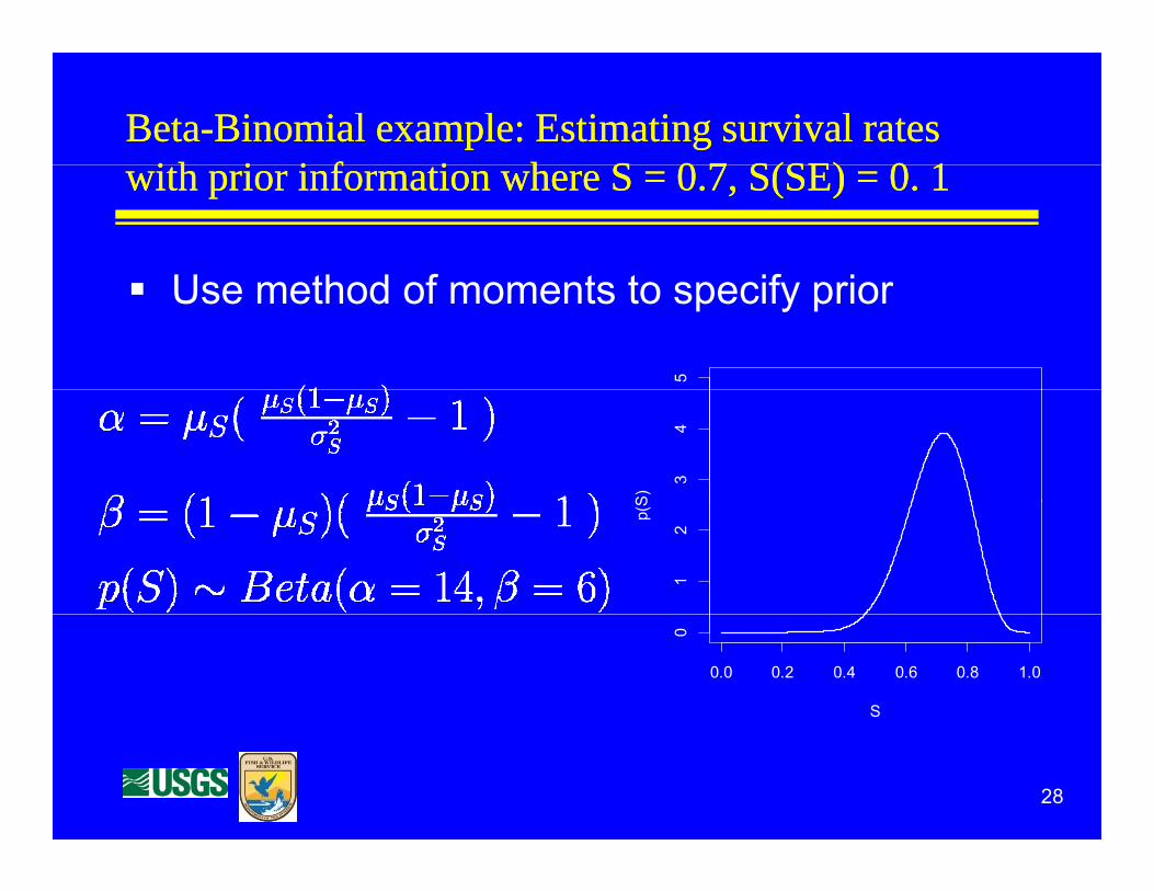
Beta-Binomial example: Estimating survival ratesi h i i f i h S 0 7 S(SE) 0 1
Beta-Binomial example: Estimating survival ratesi h i i f i h S 0 7 S(SE) 0 1with prior information where S = 0.7, S(SE) = 0. 1with prior information where S = 0.7, S(SE) = 0. 1
U th d f t t if i Use method of moments to specify prior
53
4
S)
12
p(S
0.0 0.2 0.4 0.6 0.8 1.00
S
28

Apply n = 20 transmitters in year 1, 18 i 2y = 18 survive to year 2
29

Evaluate PosteriorEvaluate Posterior
8Prior
Evaluate PosteriorEvaluate Posterior
6Posterior4
p(S)
2
0 0 0 2 0 4 0 6 0 8 1 0
0
0.0 0.2 0.4 0.6 0.8 1.0
S 30

Actual ExampleActual ExampleActual ExampleActual Example
Adaptive Harvest Management for Mid-Management for Mid
continent Mallard Ducks


How fast does learning occur?How fast does learning occur?How fast does learning occur?How fast does learning occur?

What affects the speed of learning?What affects the speed of learning?What affects the speed of learning?What affects the speed of learning?
Model structure parameter values Model structure, parameter values• Does the set include a good approximating
model?• Are parameter estimates Precise? Unbiased?
Amount of noise (stochasticity) in the systemP ti l b bilit Partial observability• Bias and precision in monitoring
Approach to optimization Approach to optimization Spatial replication
34

M d l P di tiModel Predictions
0.45
0.30.35
0.4
ensi
ty Wt = 82% Wt = 18%
0.150.2
0.25
babi
lity
De
Model 1Model 2
00.05
0.1
Prob
02 3 4 5 6 7 8 9 10 11 12 13 14 15 16
Population Size (thousands)
35
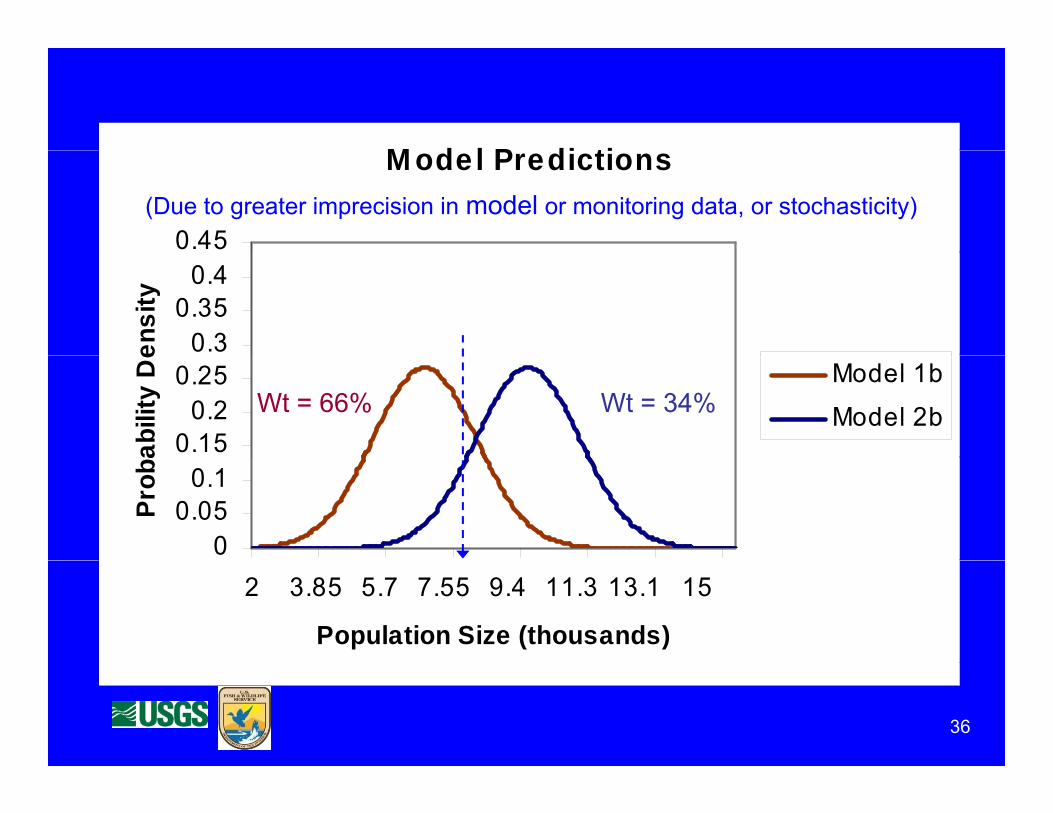
M d l P di tiM odel Predictions
0.45(Due to greater imprecision in model or monitoring data, or stochasticity)
0.30.35
0.4
ensi
ty
0.150.2
0.25
abili
ty D
e
Model 1b
Model 2bWt = 66% Wt = 34%
00.05
0.1
Prob
2 3.85 5.7 7.55 9.4 11.3 13.1 15
Population Size (thousands)
36

Model Weights(Predictions for Model 1 negatively biased)
0.350.4
0.45
sity
Wt = 50% Wt = 50%
0.20.25
0.3
bilit
y D
ens
Model 1Model 2
00.05
0.10.15
Prob
ab
02 3.35 4.7 6.05 7.4 8.75 10.1 11.5 12.8 14.2 15.5
Population Size (thousands)
37

Model Weights(Predictions for both models negatively biased)
0.350.4
0.45
sity
Wt = 18% Wt = 82%
0 150.2
0.250.3
bilit
y D
ens
Model 1Model 2
00.05
0.10.15
Prob
a
02 3.35 4.7 6.05 7.4 8.75 10.1 11.5 12.8 14.2 15.5
Population Size (thousands)
38

Can we measure the cost of poor Can we measure the cost of poor monitoring?monitoring?

Accounting for the hidden costs of measurement uncertainty in wildlife decision-making through monitoring designwildlife decision making through monitoring design
Clinton T. Moore and William L. KendallUSGS P Wildlif R h CUSGS Patuxent Wildlife Research Center
40

State-specific decision makingState-specific decision makingState specific decision makingState specific decision making
System states
5A
Decision
Reward
System State
System states• Current physical and biological
conditions of a managed system10
15
State 1B
CDecisions• Candidate management actions
14A
B
Rewards• Expected management gain for
8
3
State 2B
Cgiven decision and system state
41Moore and Kendall, TWS 2006

State-specific decision makingState-specific decision makingState specific decision makingState specific decision makingThe decision you make depends
5A
Decision
Reward
System State
y pon how you see the system
Case 1: True state is observable10
15
State 1B
CDecision “A” is best
Decision gain of 14 units
14A
B
Decision gain of 14 units
8
3
State 2B
C
True state of system
42
system
Moore and Kendall, TWS 2006
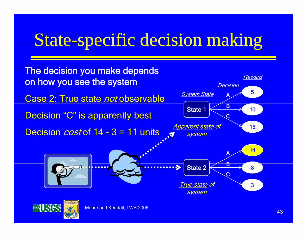
State-specific decision makingState-specific decision makingState specific decision makingState specific decision makingThe decision you make depends
5A
Decision
Reward
System State
The decision you make depends on how you see the system
Case 2: True state not observable10
15
State 1B
C
Apparent state of system
Decision “C” is apparently best
Decision cost of 14 - 3 = 11 units
14A
B
systemDecision cost of 14 3 11 units
8
3
State 2B
C
True state of system
43
system
Moore and Kendall, TWS 2006

Partial observability IPartial observability IPartial observability IPartial observability I
L d t d ti i t Leads to reduction in management returns• Best decision for apparent state differs
from that for true, unknown state• Management opportunity cost of partial
observabilityy• Measurable in units of the resource
44Moore and Kendall, TWS 2006

Partial observability and management Partial observability and management returnreturn
100%
Re
turn Opportunity costs of
misled management
ge
me
nt
RM
an
ag
0%
None Lots
Observational uncertainty
45Moore and Kendall, TWS 2006

Partial observability IIPartial observability IIPartial observability IIPartial observability II
Leads to reduction in management returnsreturns
U d t t l ( d l) t i t• Under structural (model) uncertainty, partial observability can interfere with bilit t l d l t i t dability to resolve model uncertainty and
improve management
46Moore and Kendall, TWS 2006

Partial observability and model id ifi iPartial observability and model id ifi iidentificationidentification
1el
0.8
rre
ct
mo
d
High observability
Lower observability
0 4
0.6
ne
d t
o c
or Lower observability
0.2
0.4
gh
t a
ss
ign
Lower still
0
0 2 4 6 8 10
Time
We
i
47
Time
Moore and Kendall, TWS 2006

Monitoring Program Costs: C id tiMonitoring Program Costs: C id tiConsiderationsConsiderations
C f Cost of monitoring Costs of not monitoring or monitoringCosts of not monitoring or monitoring
poorly:• Poor estimates of state for decisions• Poor estimates of state, for decisions• Slow/improper resolution of structural
uncertaintyuncertainty• Poor estimation of model parameters
48

Monitoring effort should be formally cast d i i i bl (O )
Monitoring effort should be formally cast d i i i bl (O )as a management decision variable (Oz)as a management decision variable (Oz)
Recurring decisions about:Recurring decisions about:1. Management action2. Monitoring intensity
Objective:• Include both resource conservation returns and survey costs via use
of common currency, utility thresholds, whatevery y
Could lead to adaptive monitoring design:• Value of reducing uncertainty is high monitoring intensity increases
V l f d i t i t i l it i i t it d• Value of reducing uncertainty is low monitoring intensity decreases
49Moore and Kendall, TWS 2006

Approach to OptimizationApproach to OptimizationApproach to OptimizationApproach to Optimization

Approaches to optimizationApproaches to optimizationApproaches to optimizationApproaches to optimization
Passi e ARM Passive ARM• decision made based on management objectives and current
information state (i.e. model weights)
Active ARM• Simultaneous/concurrent Active ARM
• Decision made based on management objectives, currentDecision made based on management objectives, current information state and anticipated benefit of learning (Dual Control)
• Sequential Active ARM• (1) Experimentation (learn quickly for a set of steps) with
little consideration for resource returns• (2) Passive ARM under “best” model(s) based on (1)
51

Speed of learning also function of bj i h i i i
Speed of learning also function of bj i h i i iobjectives, approach to optimizationobjectives, approach to optimization
P i l Ad tiPassively Adaptive
Actively AdaptiveActively Adaptive(anticipates benefit of learningto mgmt. objectives)
Experimentation52
p

Can learn faster with spatial replicationCan learn faster with spatial replicationCan learn faster with spatial replicationCan learn faster with spatial replication
Action A
Mgmt Area 1
Action B
Mgmt Area 2
Action B
Mgmt Area 3
Action A
Mgmt Area 4
53

Robustness: model vs. model setRobustness: model vs. model setRobustness: model vs. model setRobustness: model vs. model set Suggestion: don’t discard a hypothesis too gg yp
quickly based on poor model predictive performance (model may not properly capture hypothesis, may be constructed with poor ypo es s, ay be co s uc ed pooparameter estimates, etc.)
If i ht bi ( b i If weights are ambiguous (e.g. bouncing around over time), but model set predicts well, then no need to panic
If model set predicts poorly, then really need to revise or add models (double loop learning)
54
revise or add models (double-loop learning)

Conclusions About Learning: IConclusions About Learning: IConclusions About Learning: IConclusions About Learning: I
Learning is hallmark of ARM Learning is hallmark of ARM
It is not appropriate to label a management It is not appropriate to label a management program as “adaptive” without a clear mechanism for incorporation of learning to p gimprove subsequent management
The purpose of learning in ARM is to provide increased returns by improving predictions across entire state space
55
across entire state space

Conclusions About Learning: IIConclusions About Learning: IIConclusions About Learning: IIConclusions About Learning: II Bayes formula is natural vehicle for “learning” in ARM
( d i i )(and in science) Rate of “learning” depends on many factors, e.g.,
• Stochastic variation of model predictionsp• Variation among model-based predictions for members of
model set• Partial observability• Approach to optimization
True learning depends on how well at least one member of the model set captures underlyingmember of the model set captures underlying mechanisms (so we still need to think)
56

57

Why bother to learn in ARM?Why bother to learn in ARM?Why bother to learn in ARM?Why bother to learn in ARM?
Expected value of perfect information (EVPI)Expected value of perfect information (EVPI) compares:• weighted average of model-specific e g ed a e age o ode spec c
maximum values, across models (omniscience)
• maximum of an average of values (based on average model performance; value under
)best nonadaptive decision)

Why bother to learn in ARM?Why bother to learn in ARM?Why bother to learn in ARM?Why bother to learn in ARM?
![100percent renewables-short version-ires bonn 2007 V2.ppt ......Microsoft PowerPoint - 100percent_renewables-short_version-ires_bonn_2007 V2.ppt [Kompatibilitätsmodus] Author Ebi](https://img.pdfslide.us/doc/110x75/60f94ca0a74edf3e375f3d19/100percent-renewables-short-version-ires-bonn-2007-v2ppt-microsoft-powerpoint.jpg)


![v2[6].ppt (Read-Only)](https://img.pdfslide.us/doc/110x75/586e123a1a28ab5f288bd89a/v26ppt-read-only.jpg)