Embed Size (px)
Citation preview
In the name of GodIn the name of God
Network Flows
6. Lagrangian Relaxation
6.3 Lagrangian Relaxation and Integer 6.3 Lagrangian Relaxation and Integer
Programming
Fall 2010Instructor: Dr. Masoud Yaghini
Outline
� Integer Programming
� Branch-and-Bound Technique
� Applications of Lagrangian Relaxation in Integer
Programming
� Applications of Lagrangian Relaxation in � Applications of Lagrangian Relaxation in
Uncapacitated Network Design
Integer Programming
Integer Programming
� Integer Programming (IP) Problem
– A linear programming problem in which the decision
variables are required to have integer values
– The mathematical model for integer programming is the
linear programming model with the one additional
restriction that the variables must have integer valuesrestriction that the variables must have integer values
� Integer Linear Programming problem
– The more complete name of IP problem but the adjective
linear normally is dropped except when this problem is
contrasted with integer nonlinear programming problem
Integer Programming
� Mixed Integer Programming (MIP)
– If only some of the variables are required to have integer
values and the divisibility assumption holds for the rest
variables
� Pure Integer Programming
– If all the variables are required to have integer values– If all the variables are required to have integer values
� Binary Integer Programming (BIP)
– or 0–1 integer programming problems
– IP problems that contain only binary variables
Branch-and-Bound Technique
Branch-and-Bound Technique
� Branch-and-bound technique
– The basic concept is to divide and conquer.
– Since the original “large” problem is too difficult to be
solved directly, it is divided into smaller and smaller
subproblems until these subproblems can be conquered.
Branch-and-Bound Technique
� Branch-and-bound technique steps
– The dividing (branching)
� partitioning the entire set of feasible solutions into smaller and
smaller subsets.
– The bounding
� how good the best solution in the subset can be� how good the best solution in the subset can be
– The conquering ( fathoming)
� discarding the subset if its bound indicates that it cannot possibly
contain an optimal solution for the original problem.
Branch-and-Bound Technique
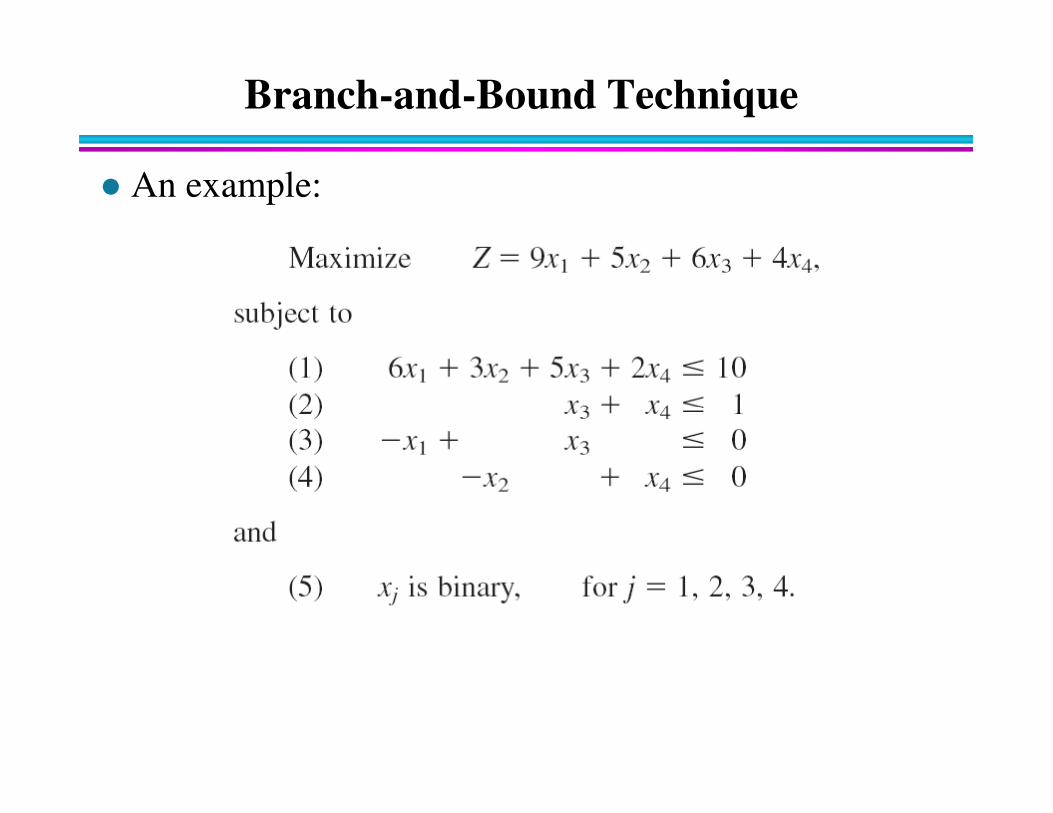
� An example:
Branch-and-Bound Technique
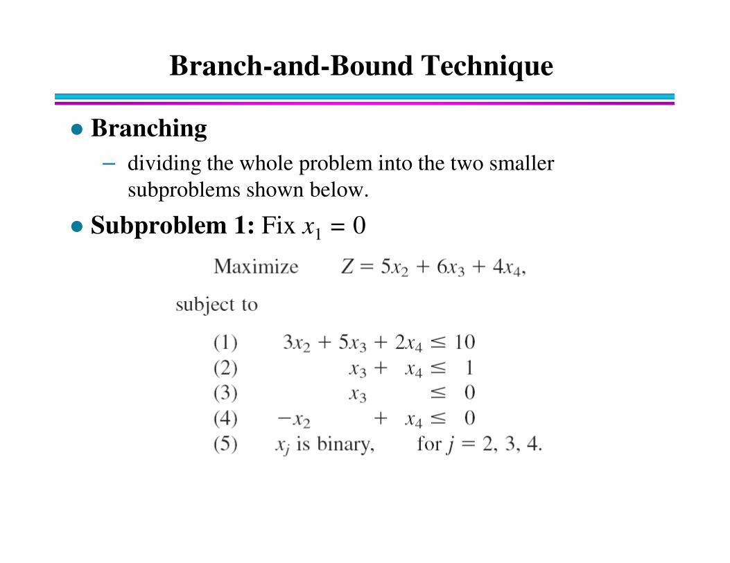
� Branching
– dividing the whole problem into the two smaller
subproblems shown below.
� Subproblem 1: Fix x1 = 0
Branch-and-Bound Technique
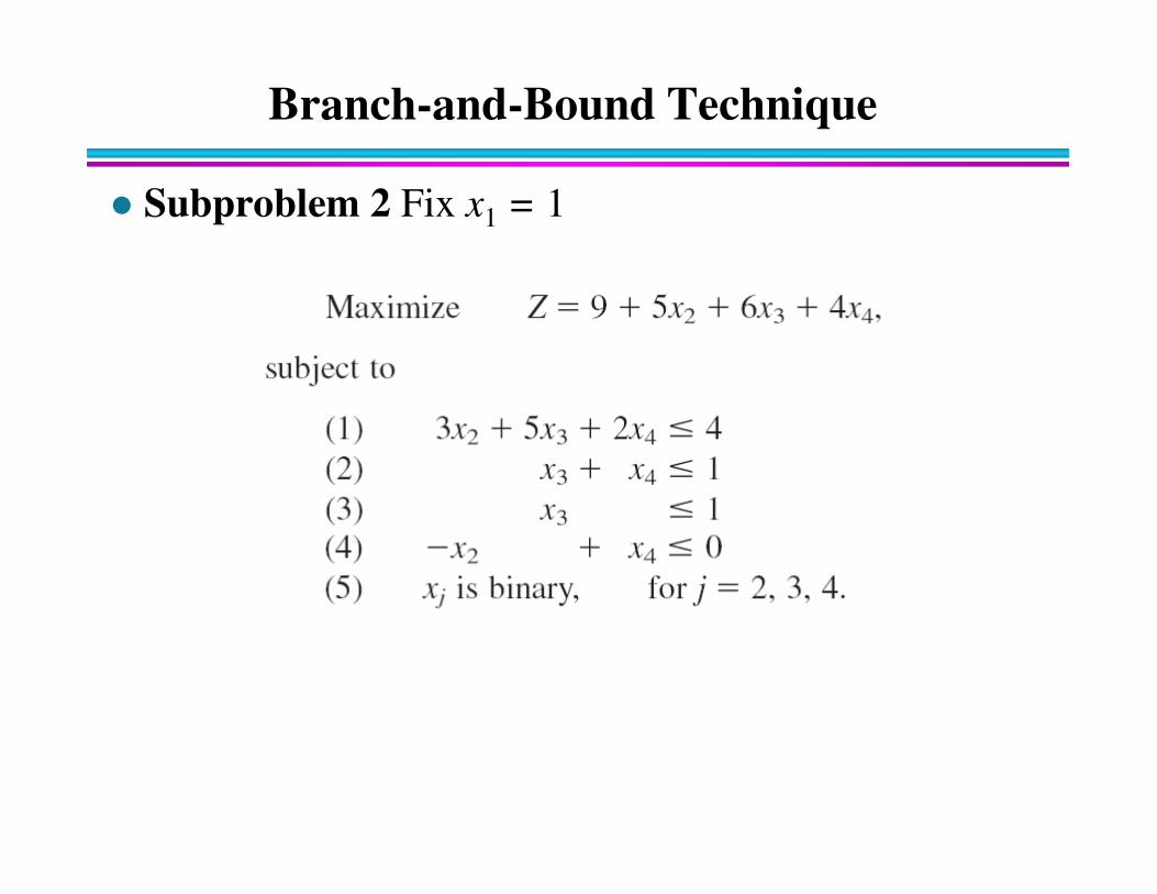
� Subproblem 2 Fix x1 = 1
Branch-and-Bound Technique
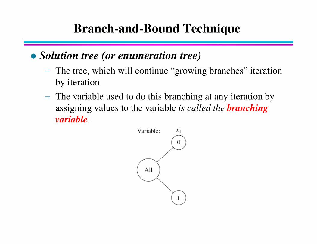
� Solution tree (or enumeration tree)
– The tree, which will continue “growing branches” iteration
by iteration
– The variable used to do this branching at any iteration by
assigning values to the variable is called the branching
variable.variable.
Branch-and-Bound Technique
� Selecting branching variables
– Sophisticated methods for selecting branching variables are
an important part of some branch-and-bound algorithms
– for simplicity, we select them in their natural order—x1, x2,
. . . , xn
Branch-and-Bound Technique
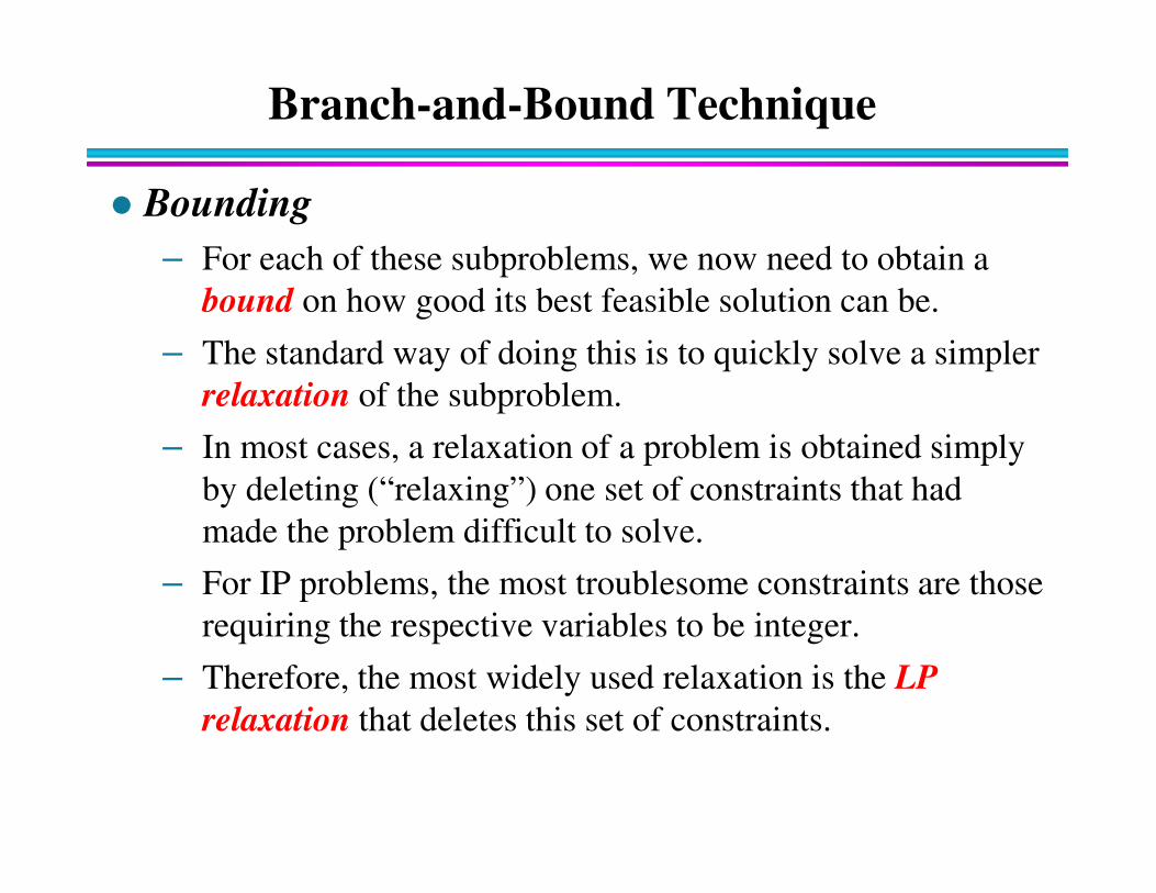
� Bounding
– For each of these subproblems, we now need to obtain a
bound on how good its best feasible solution can be.
– The standard way of doing this is to quickly solve a simpler
relaxation of the subproblem.
– In most cases, a relaxation of a problem is obtained simply – In most cases, a relaxation of a problem is obtained simply
by deleting (“relaxing”) one set of constraints that had
made the problem difficult to solve.
– For IP problems, the most troublesome constraints are those
requiring the respective variables to be integer.
– Therefore, the most widely used relaxation is the LP
relaxation that deletes this set of constraints.
Branch-and-Bound Technique
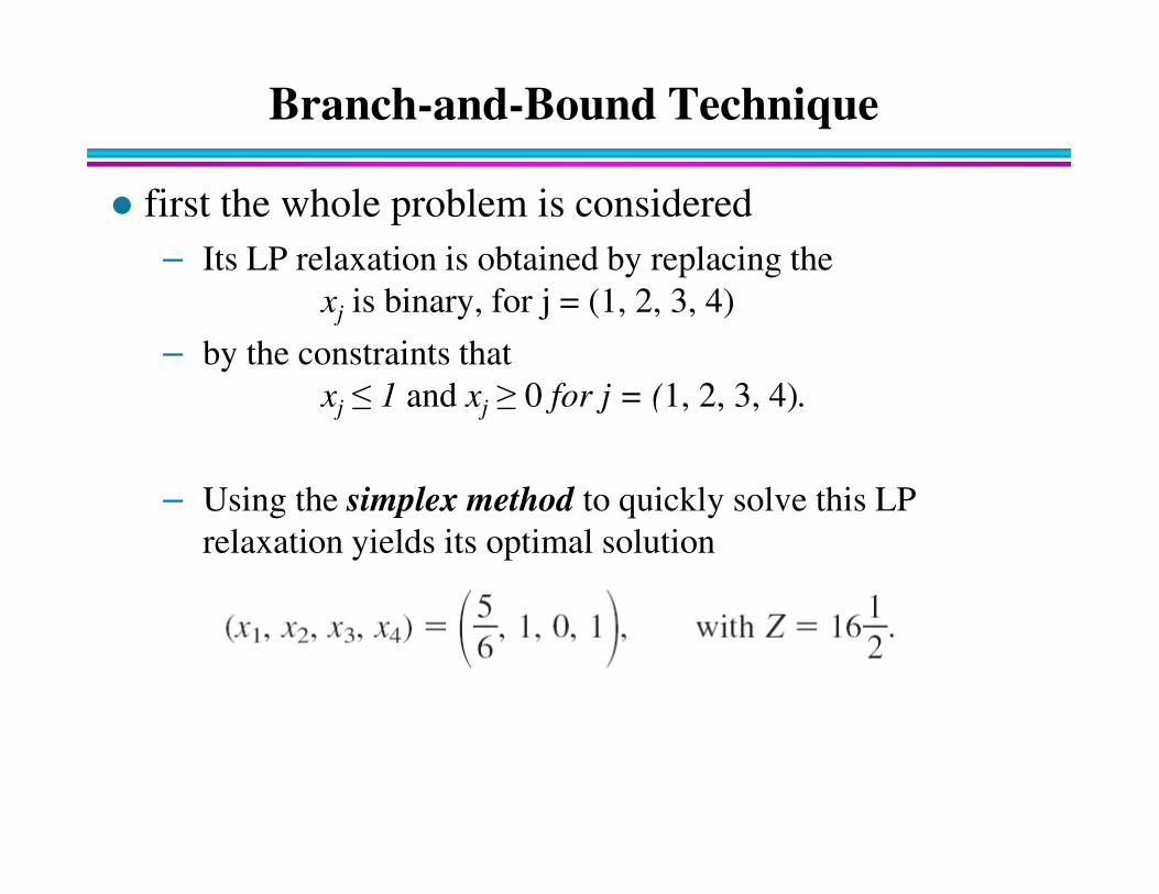
� first the whole problem is considered
– Its LP relaxation is obtained by replacing the
xj is binary, for j = (1, 2, 3, 4)
– by the constraints that
xj ≤ 1 and xj ≥ 0 for j = (1, 2, 3, 4).
– Using the simplex method to quickly solve this LP
relaxation yields its optimal solution
Branch-and-Bound Technique
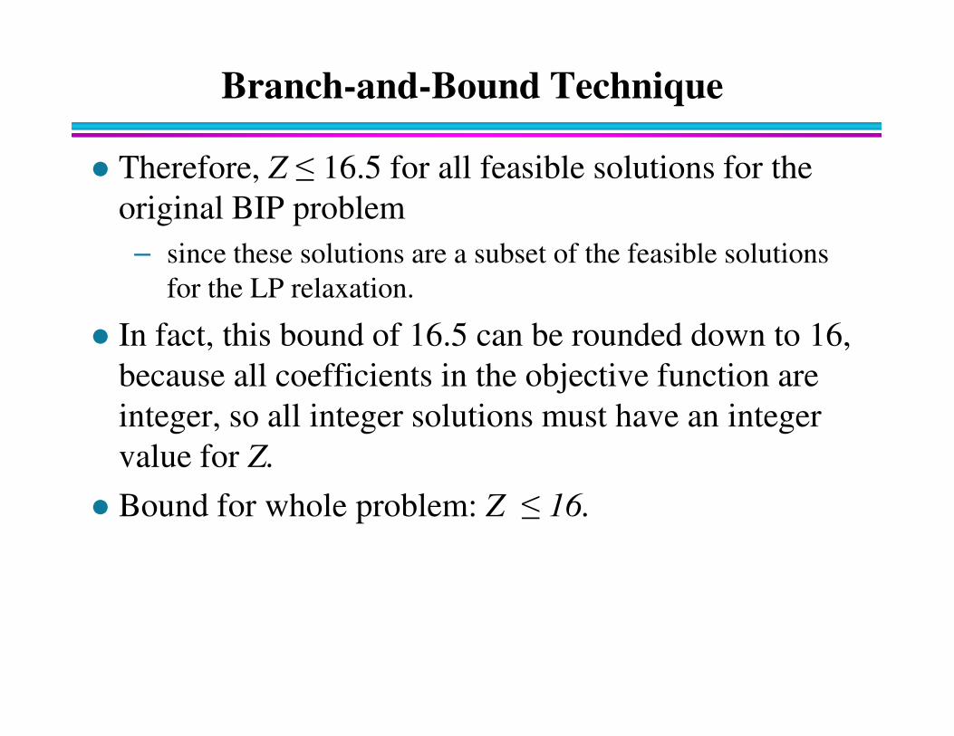
� Therefore, Z ≤ 16.5 for all feasible solutions for the
original BIP problem
– since these solutions are a subset of the feasible solutions
for the LP relaxation.
� In fact, this bound of 16.5 can be rounded down to 16,
because all coefficients in the objective function are because all coefficients in the objective function are
integer, so all integer solutions must have an integer
value for Z.
� Bound for whole problem: Z ≤ 16.
Branch-and-Bound Technique
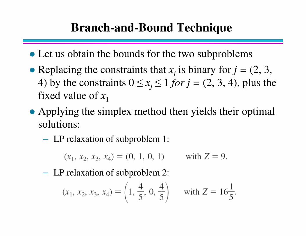
� Let us obtain the bounds for the two subproblems
� Replacing the constraints that xj is binary for j = (2, 3,
4) by the constraints 0 ≤ xj ≤ 1 for j = (2, 3, 4), plus the
fixed value of x1
� Applying the simplex method then yields their optimal
solutions:solutions:
– LP relaxation of subproblem 1:
– LP relaxation of subproblem 2:
Branch-and-Bound Technique
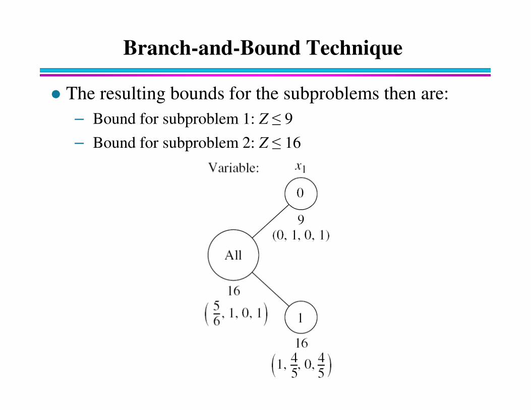
� The resulting bounds for the subproblems then are:
– Bound for subproblem 1: Z ≤ 9
– Bound for subproblem 2: Z ≤ 16

Branch-and-Bound Technique
� Three ways of fathoming a subproblem
– (1) The optimal solution for its LP relaxation is an integer
solution.
� If necessary, the best-so-far integer solution or incumbent (Z*)
must be updated.
– (2) Its bound is less than or equal best-so-far integer – (2) Its bound is less than or equal best-so-far integer
solution
– (3) A subproblem’s LP relaxation has no feasible solutions
Branch-and-Bound Technique
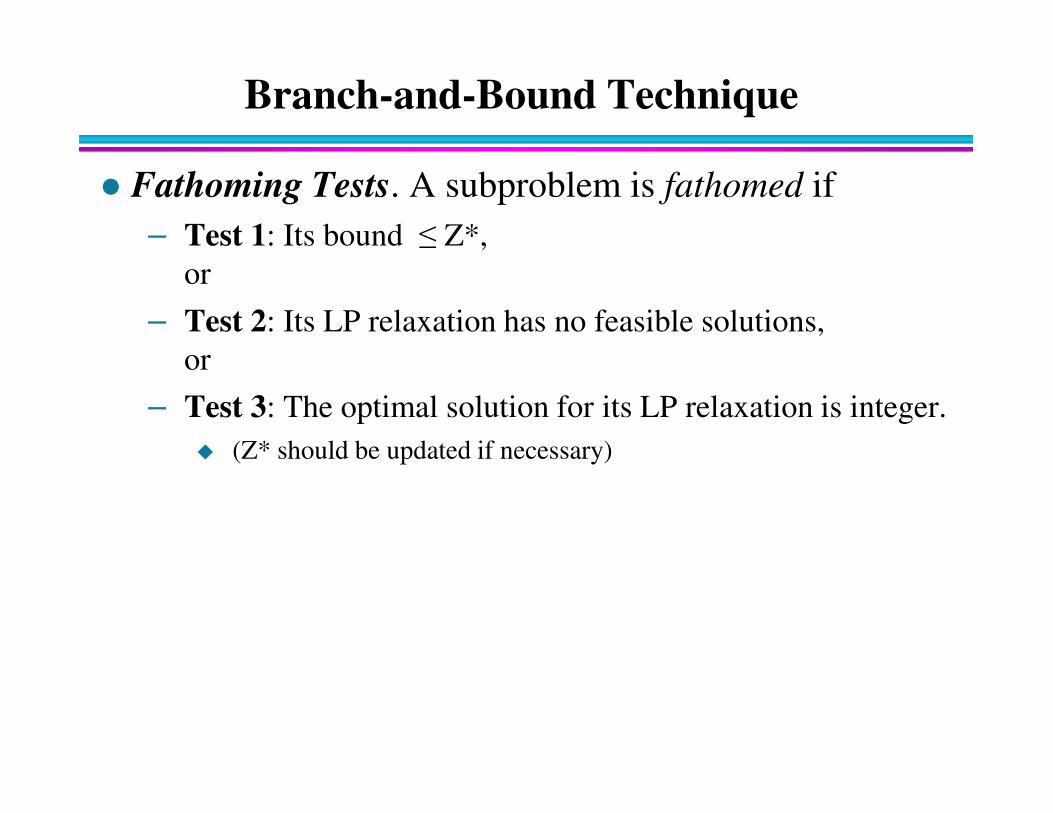
� Fathoming Tests. A subproblem is fathomed if
– Test 1: Its bound ≤ Z*,
or
– Test 2: Its LP relaxation has no feasible solutions,
or
– Test 3: The optimal solution for its LP relaxation is integer.– Test 3: The optimal solution for its LP relaxation is integer.
� (Z* should be updated if necessary)
Branch-and-Bound Technique
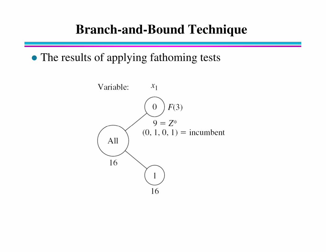
� The results of applying fathoming tests
Branch-and-Bound Technique
� Optimality test:
– Stop when there are no remaining subproblems;
– the current incumbent is optimal.
Integer Programming
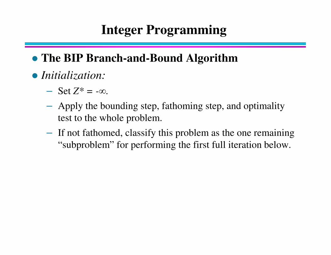
� The BIP Branch-and-Bound Algorithm
� Initialization:
– Set Z* = -∞.
– Apply the bounding step, fathoming step, and optimality
test to the whole problem.
– If not fathomed, classify this problem as the one remaining – If not fathomed, classify this problem as the one remaining
“subproblem” for performing the first full iteration below.
Branch-and-Bound Technique
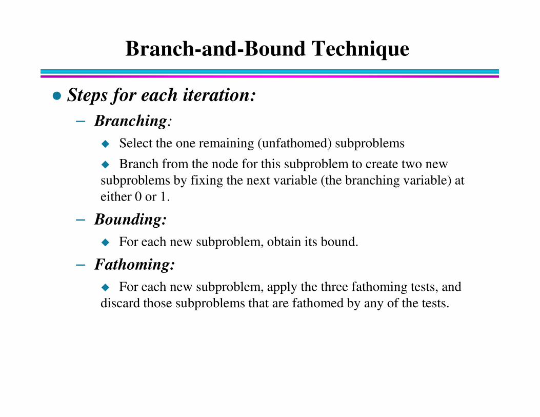
� Steps for each iteration:
– Branching:
� Select the one remaining (unfathomed) subproblems
� Branch from the node for this subproblem to create two new
subproblems by fixing the next variable (the branching variable) at
either 0 or 1.
– Bounding:
� For each new subproblem, obtain its bound.
– Fathoming:
� For each new subproblem, apply the three fathoming tests, and
discard those subproblems that are fathomed by any of the tests.
Branch-and-Bound Technique
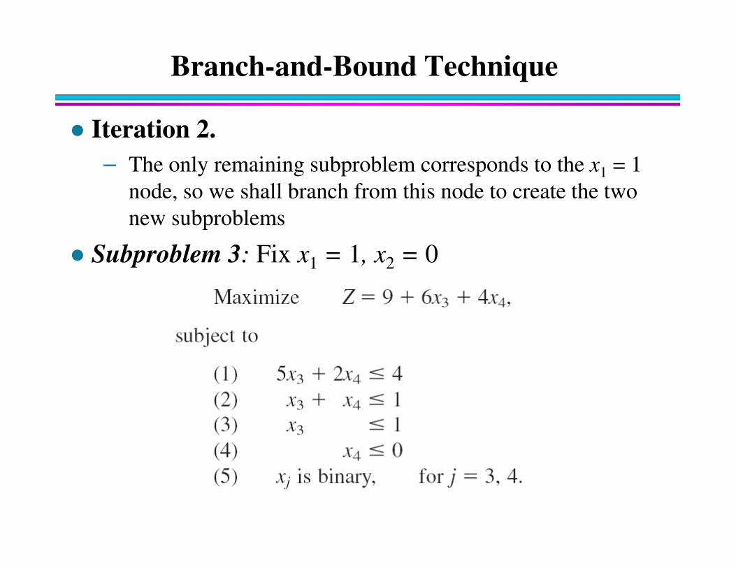
� Iteration 2.
– The only remaining subproblem corresponds to the x1 = 1
node, so we shall branch from this node to create the two
new subproblems
� Subproblem 3: Fix x1 = 1, x2 = 0
Branch-and-Bound Technique
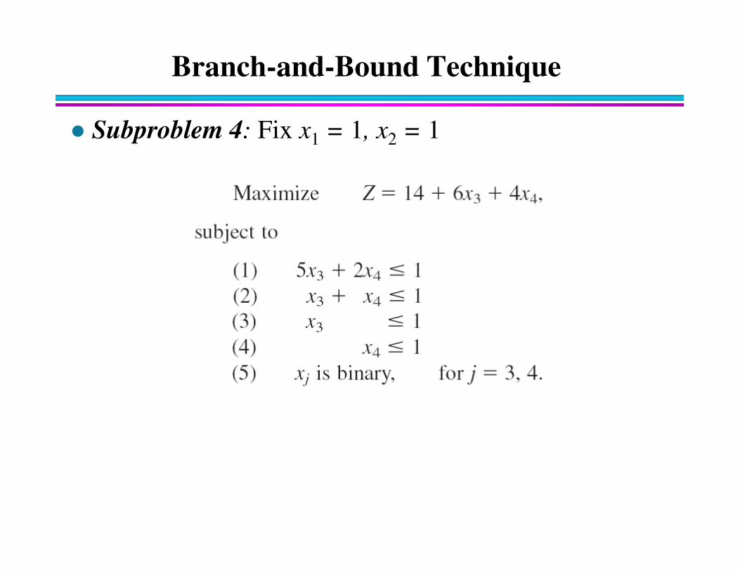
� Subproblem 4: Fix x1 = 1, x2 = 1
Branch-and-Bound Technique
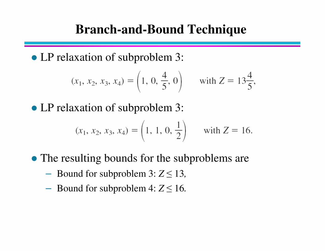
� LP relaxation of subproblem 3:
� LP relaxation of subproblem 3:
� The resulting bounds for the subproblems are
– Bound for subproblem 3: Z ≤ 13,
– Bound for subproblem 4: Z ≤ 16.
Branch-and-Bound Technique
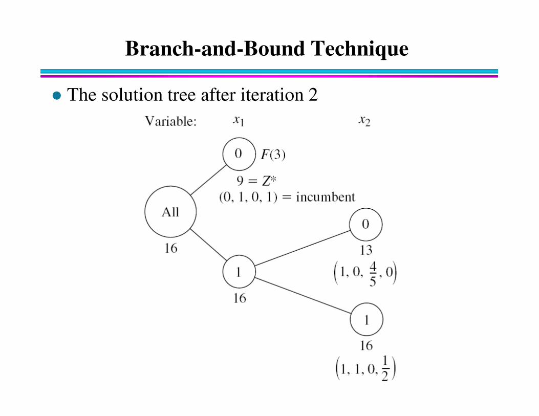
� The solution tree after iteration 2
Branch-and-Bound Technique
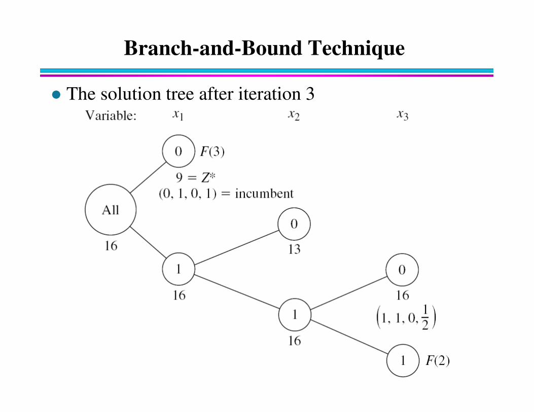
� The solution tree after iteration 3
Integer Programming
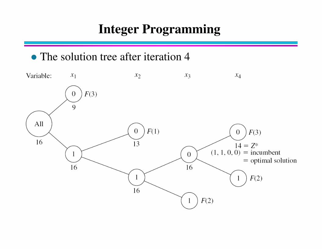
� The solution tree after iteration 4
Applications of Lagrangian Relaxation in
Integer Programming Integer Programming
Lagrangian Relaxation and Integer Programming
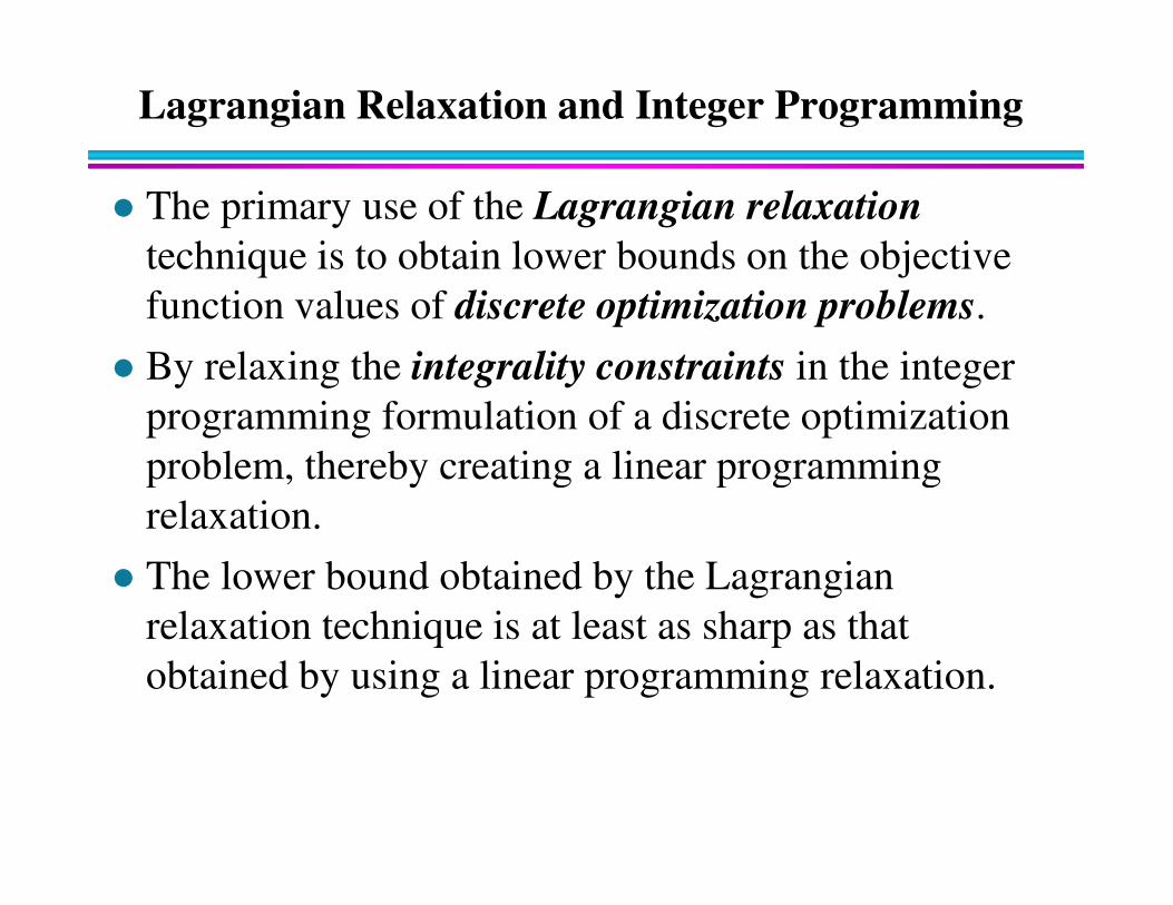
� The primary use of the Lagrangian relaxation
technique is to obtain lower bounds on the objective
function values of discrete optimization problems.
� By relaxing the integrality constraints in the integer
programming formulation of a discrete optimization
problem, thereby creating a linear programming problem, thereby creating a linear programming
relaxation.
� The lower bound obtained by the Lagrangian
relaxation technique is at least as sharp as that
obtained by using a linear programming relaxation.
Lagrangian Relaxation and Integer Programming
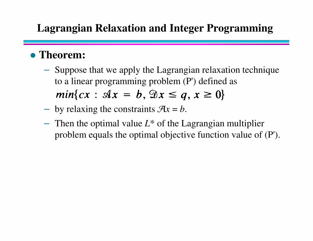
� Theorem:
– Suppose that we apply the Lagrangian relaxation technique
to a linear programming problem (P') defined as
– by relaxing the constraints Ax = b.
– Then the optimal value L* of the Lagrangian multiplier – Then the optimal value L* of the Lagrangian multiplier
problem equals the optimal objective function value of (P').
Lagrangian Relaxation and Integer Programming
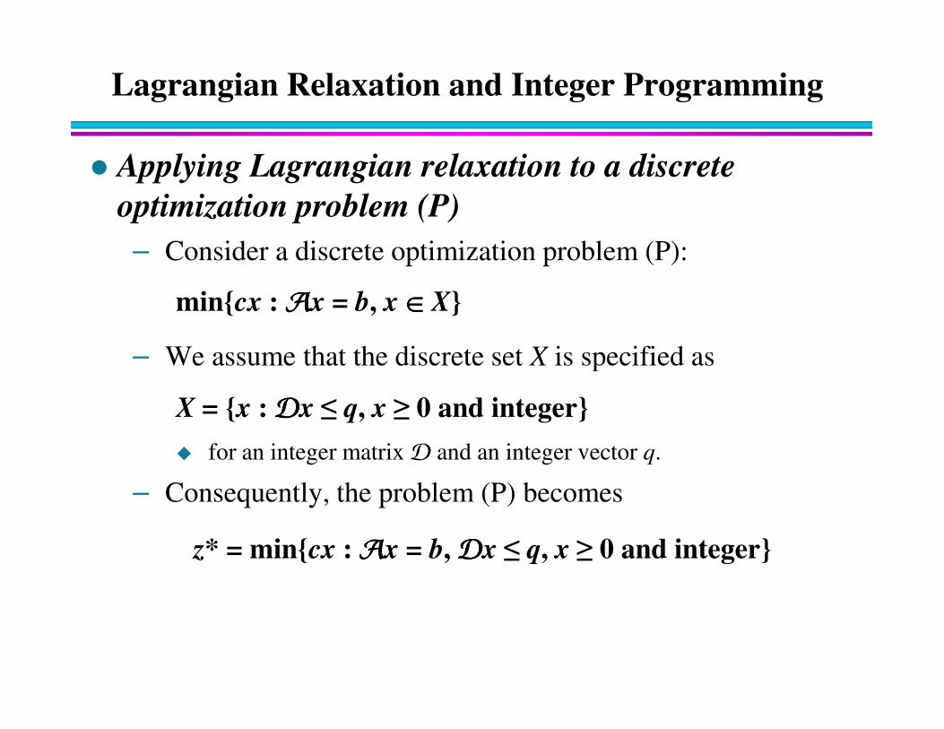
� Applying Lagrangian relaxation to a discrete
optimization problem (P)
– Consider a discrete optimization problem (P):
min{cx : AAAAx = b, x œœœœ X}
– We assume that the discrete set X is specified as – We assume that the discrete set X is specified as
X = {x : DDDDx ≤ q, x ≥ 0 and integer}
� for an integer matrix D and an integer vector q.
– Consequently, the problem (P) becomes
z* = min{cx : AAAAx = b, DDDDx ≤ q, x ≥ 0 and integer}

Lagrangian Relaxation and Integer Programming
� Linear Programming Relaxation
– Let (LP) denote the linear programming relaxation of the
problem (P) and let zo denote its optimal objective function
value:
zo = min{cx : AAAAx = b, DDDDx ≤ q, x ≥ 0} (LP)
– Clearly, zo ≤ z* because the set of feasible solutions of (P)
lies within the set of feasible solutions of (LP).
– Therefore, the linear programming relaxation provides a
valid lower bound on the optimal objective function value
of (P).
Lagrangian Relaxation and Integer Programming
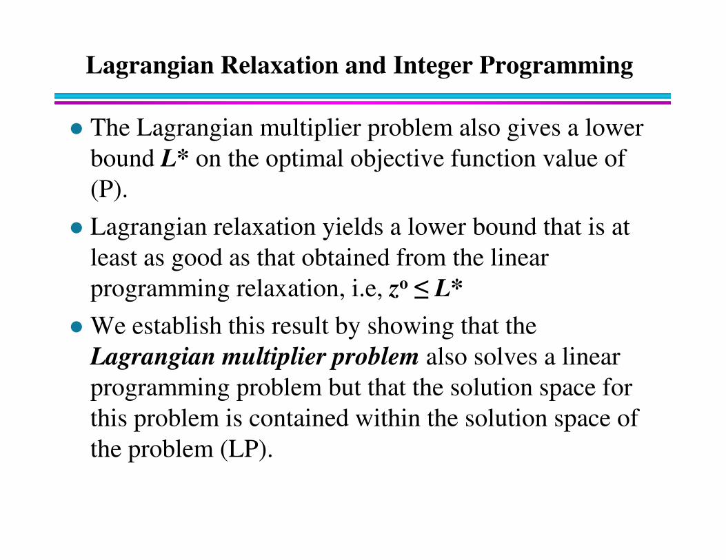
� The Lagrangian multiplier problem also gives a lower
bound L* on the optimal objective function value of
(P).
� Lagrangian relaxation yields a lower bound that is at
least as good as that obtained from the linear
programming relaxation, i.e, zo ≤ L*programming relaxation, i.e, zo ≤ L*
� We establish this result by showing that the
Lagrangian multiplier problem also solves a linear
programming problem but that the solution space for
this problem is contained within the solution space of
the problem (LP).
Lagrangian Relaxation and Integer Programming
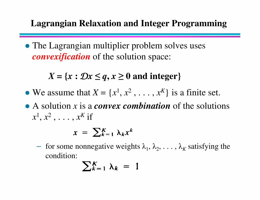
� The Lagrangian multiplier problem solves uses
convexification of the solution space:
X = {x : DDDDx ≤ q, x ≥ 0 and integer}
� We assume that X = {x1, x2 , . . . , xK} is a finite set.
� A solution x is a convex combination of the solutions
x1, x2 , . . . , xK if
– for some nonnegative weights λ1, λ2, . . . , λK satisfying the
condition:
Lagrangian Relaxation and Integer Programming
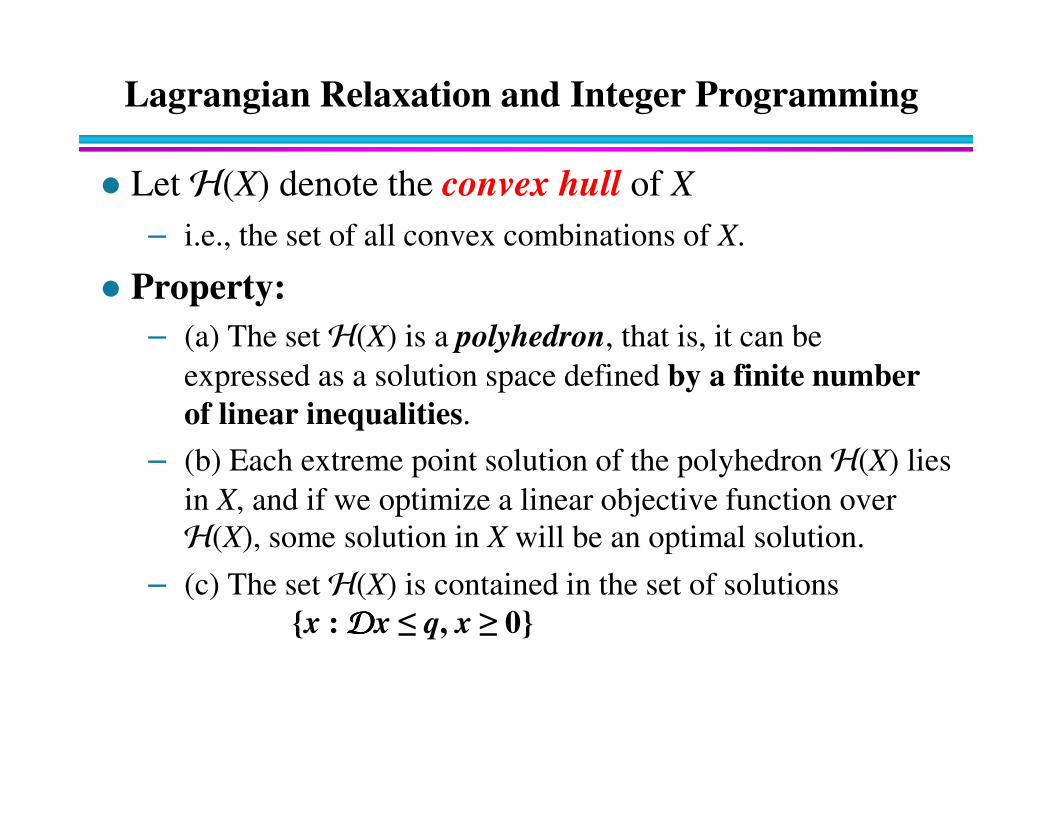
� Let H(X) denote the convex hull of X
– i.e., the set of all convex combinations of X.
� Property:
– (a) The set H(X) is a polyhedron, that is, it can be
expressed as a solution space defined by a finite number
of linear inequalities. of linear inequalities.
– (b) Each extreme point solution of the polyhedron H(X) lies
in X, and if we optimize a linear objective function over
H(X), some solution in X will be an optimal solution.
– (c) The set H(X) is contained in the set of solutions
{x : DDDDx ≤ q, x ≥ 0}
Lagrangian Relaxation and Integer Programming
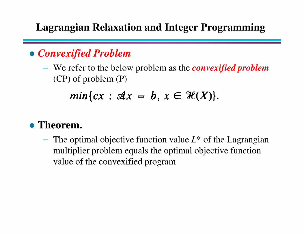
� Convexified Problem
– We refer to the below problem as the convexified problem
(CP) of problem (P)
� Theorem.
– The optimal objective function value L* of the Lagrangian
multiplier problem equals the optimal objective function
value of the convexified program

Lagrangian Relaxation and Integer Programming
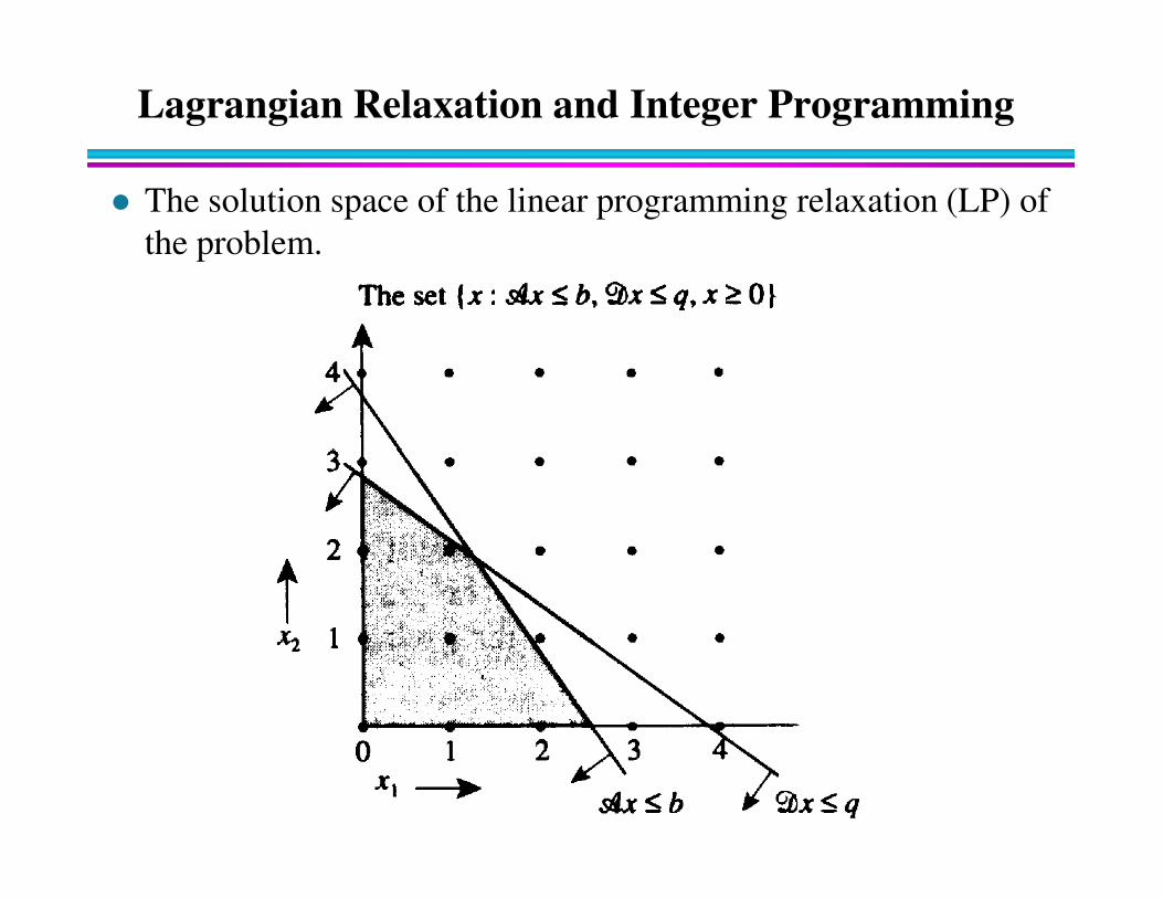
� An Example: We consider a two-variable problem with the
constraints Ax ≤ b and Ax ≤ q :
Lagrangian Relaxation and Integer Programming
� The solution space of the linear programming relaxation (LP) of
the problem.
Lagrangian Relaxation and Integer Programming
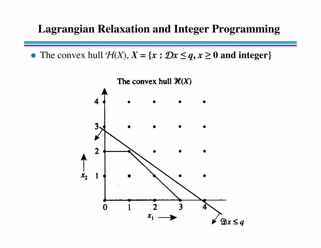
� The convex hull H(X), X = {x : DDDDx ≤ q, x ≥ 0 and integer}
Lagrangian Relaxation and Integer Programming
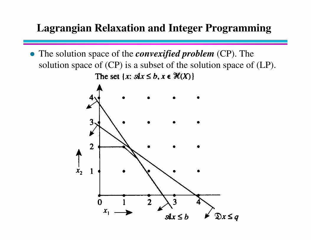
� The solution space of the convexified problem (CP). The
solution space of (CP) is a subset of the solution space of (LP).
Lagrangian Relaxation and Integer Programming
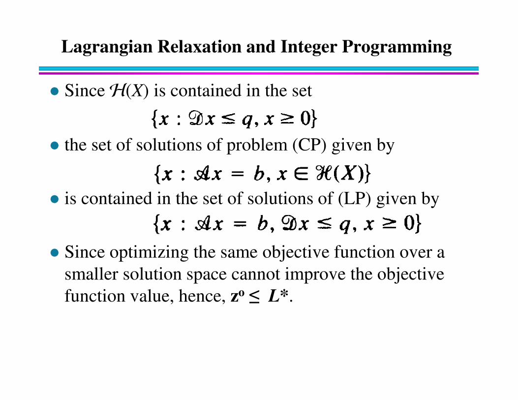
� Since H(X) is contained in the set
� the set of solutions of problem (CP) given by
� is contained in the set of solutions of (LP) given by � is contained in the set of solutions of (LP) given by
� Since optimizing the same objective function over a
smaller solution space cannot improve the objective
function value, hence, zo ≤ L*.
Lagrangian Relaxation and Integer Programming
� Theorem:
– When applied to an integer program stated in minimization
form, the lower bound obtained by the Lagrangian
relaxation technique is always as large (or, sharp) as the
bound obtained by the linear programming relaxation of the
problem; that is, zo ≤ L*.
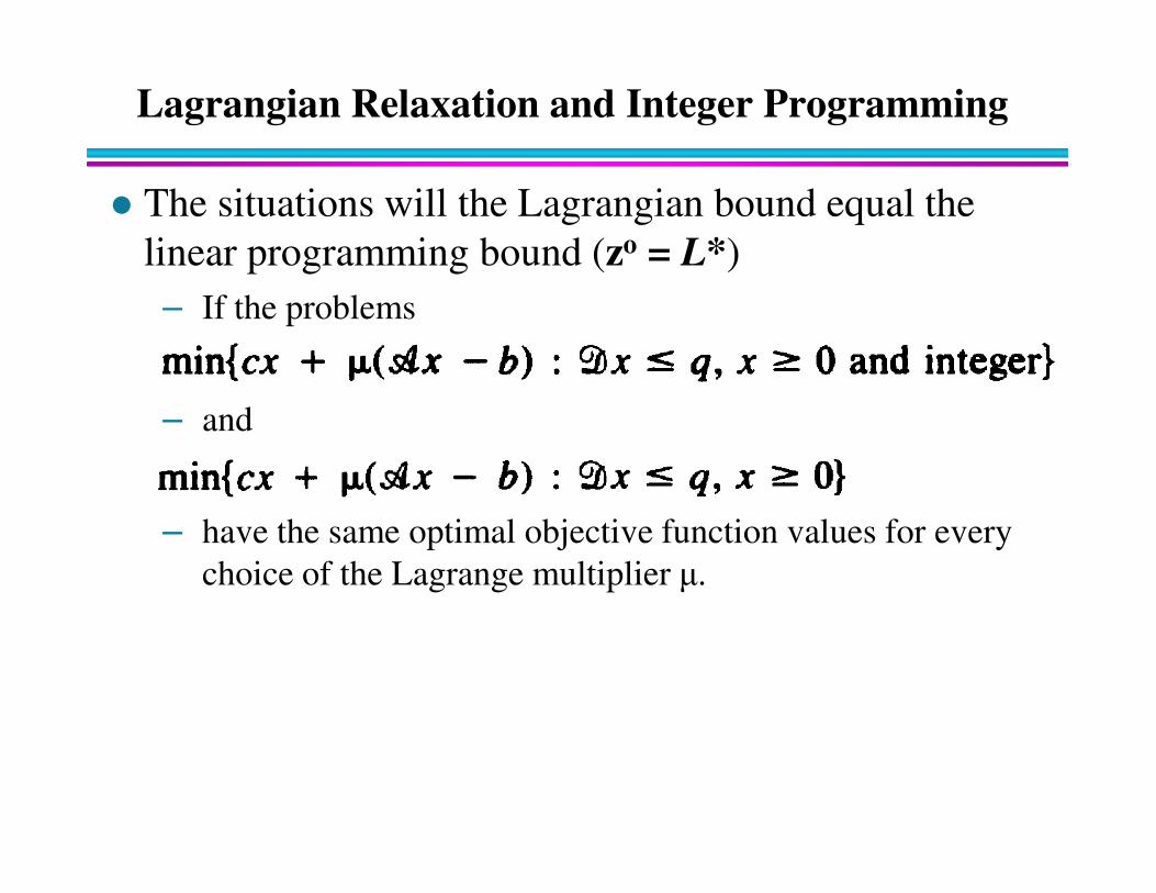
Lagrangian Relaxation and Integer Programming
� The situations will the Lagrangian bound equal the
linear programming bound (zo = L*)
– If the problems
– and
– have the same optimal objective function values for every
choice of the Lagrange multiplier µ.
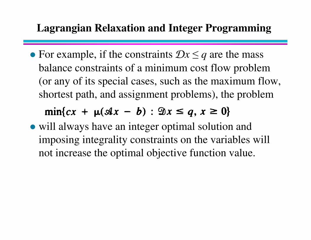
Lagrangian Relaxation and Integer Programming
� For example, if the constraints Dx ≤ q are the mass
balance constraints of a minimum cost flow problem
(or any of its special cases, such as the maximum flow,
shortest path, and assignment problems), the problem
will always have an integer optimal solution and � will always have an integer optimal solution and
imposing integrality constraints on the variables will
not increase the optimal objective function value.

Applications of Lagrangian Relaxation in
Uncapacitated Network Design Uncapacitated Network Design
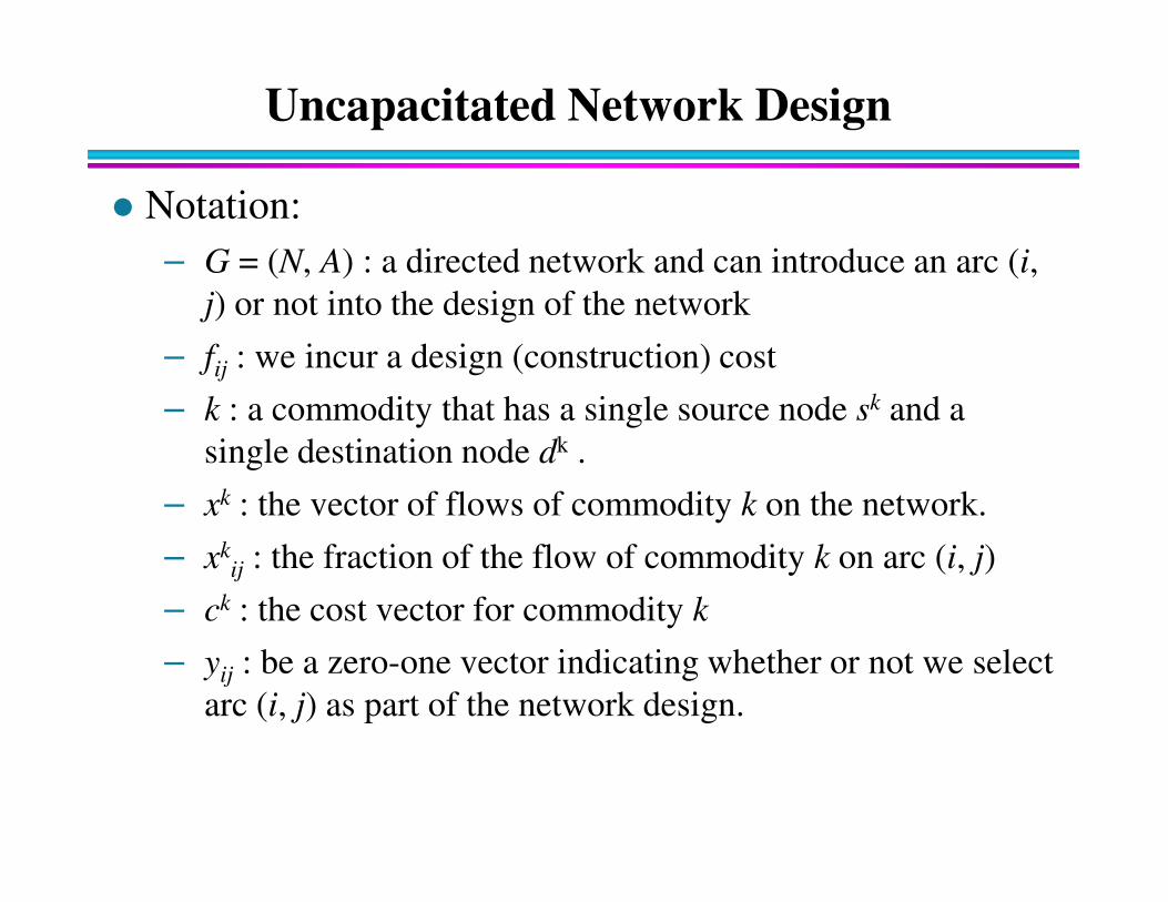
Uncapacitated Network Design
� Notation:
– G = (N, A) : a directed network and can introduce an arc (i,
j) or not into the design of the network
– fij : we incur a design (construction) cost
– k : a commodity that has a single source node sk and a
single destination node dk . single destination node dk .
– xk : the vector of flows of commodity k on the network.
– xkij : the fraction of the flow of commodity k on arc (i, j)
– ck : the cost vector for commodity k
– yij : be a zero-one vector indicating whether or not we select
arc (i, j) as part of the network design.
Uncapacitated Network Design
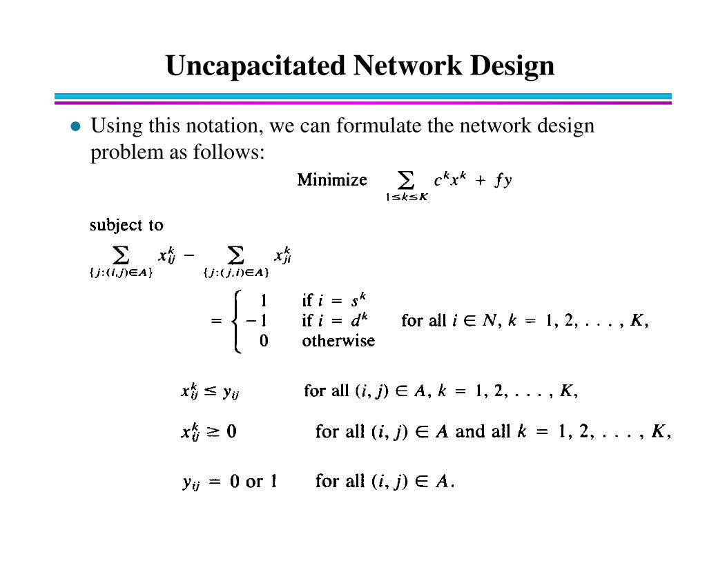
� Using this notation, we can formulate the network design
problem as follows:
Uncapacitated Network Design
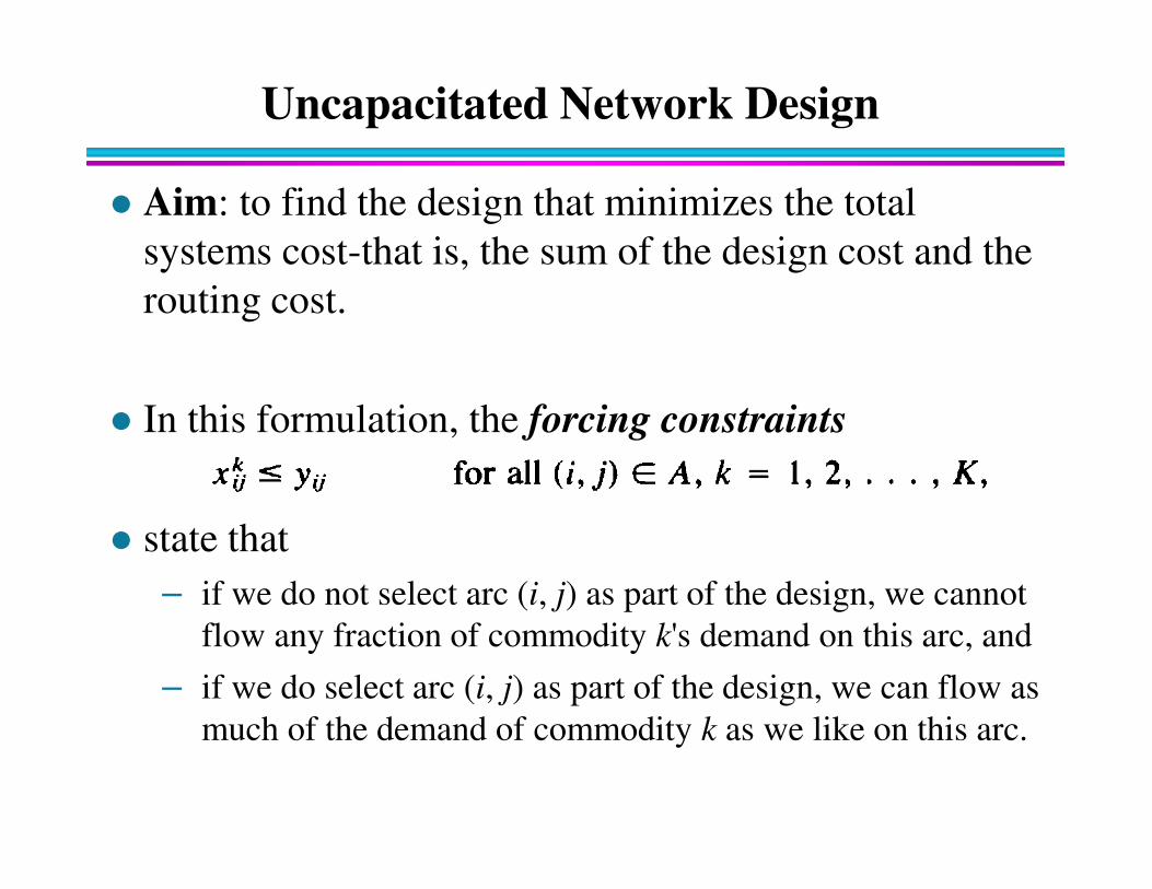
� Aim: to find the design that minimizes the total
systems cost-that is, the sum of the design cost and the
routing cost.
� In this formulation, the forcing constraints
� state that
– if we do not select arc (i, j) as part of the design, we cannot
flow any fraction of commodity k's demand on this arc, and
– if we do select arc (i, j) as part of the design, we can flow as
much of the demand of commodity k as we like on this arc.
Uncapacitated Network Design
� Note that if we remove the forcing constraints from
this model, the resulting model in the flow variables xk
decomposes into a set of independent shortest path
problems, one for each commodity k.
� Consequently, the model is another attractive
candidate for the application of Lagrangian relaxation. candidate for the application of Lagrangian relaxation.
Uncapacitated Network Design
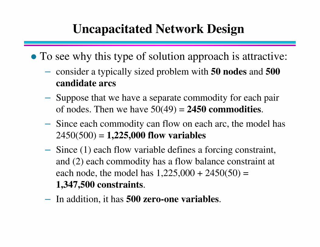
� To see why this type of solution approach is attractive:
– consider a typically sized problem with 50 nodes and 500
candidate arcs
– Suppose that we have a separate commodity for each pair
of nodes. Then we have 50(49) = 2450 commodities.
– Since each commodity can flow on each arc, the model has – Since each commodity can flow on each arc, the model has
2450(500) = 1,225,000 flow variables
– Since (1) each flow variable defines a forcing constraint,
and (2) each commodity has a flow balance constraint at
each node, the model has 1,225,000 + 2450(50) =
1,347,500 constraints.
– In addition, it has 500 zero-one variables.
Uncapacitated Network Design
� So even as a linear program, this model is very big.
� By decomposing the problem, however, for each
choice of the vector of Lagrange multipliers, we will
solve 2450 small shortest path problems.
The End