Theory of Integer Programming

Debasis Mishra∗

April 20, 2011

1 Integer Programming

1.1 What is an Integer Program?

Suppose that we have a linear program

maxcx : Ax ≤ b, x ≥ 0 (P)

where A is an m × n matrix, c an n-dimensional row vector, b an m-dimensional column

vector, and x an n-dimensional column vector of variables. Now, we add in the restriction

that some of the variables in (P) must take integer values.

If some but not all variables are integer, we have a Mixed Integer Program (MIP),

written as

max cx + hy

s.t. (MIP)

Ax + Gy ≤ b

x ≥ 0

y ≥ 0 and integer.

where A is again m × n matrix, G is m × p, h is a p row vector, and y is a p column vector

of integer variables.

If all variables are integer, then we have an Integer Program (IP), written as

max cx

s.t. (IP)

Ax ≤ b

x ≥ 0 and integer.

∗Planning Unit, Indian Statistical Institute, 7 Shahid Jit Singh Marg, New Delhi 110016, India, E-mail:

dmishra@isid.ac.in

1

If the variables in an IP is restricted to take values in 0, 1 then the IP is called a Binary

Integer Program (BIP).

1.2 Common Integer Programming Problems

1.2.1 The Assignment Problem

There is a set of indivisible goods G = 1, . . . , n. The goods need to be assigned to a set

of buyers B = 1, . . . , m. Each buyer can be assigned at most one good from G. If good

j ∈ G is assigned to buyer i ∈ B, then it generates a value of vij . The objective is to find an

assignment that maximizes the total value generated.

Define variables xij to denote if buyer i is assigned good j, i.e., xij = 1 if i is assigned

j, and zero otherwise. So, it is a binary variable. The constraints should ensure that no

good is assigned to more than one buyer and no buyer is assigned more than one good. The

objective function is to maximize∑

i∈B

∑

j∈G vijxij . Hence, the formulation is as follows:

max∑

i∈B

∑

j∈G

vijxij

s.t. (AP)∑

i∈B

xij ≤ 1 ∀ j ∈ G

∑

j∈G

xij ≤ 1 ∀ i ∈ B

xij ∈ 0, 1 ∀ i ∈ B, ∀ j ∈ G.

1.2.2 The 0 − 1 Knapsack Problem

There is a budget b available for investment in n projects. aj is the required investment of

project j. cj is the expected profit from project j. The goal is to choose a set of projects to

maximize expected profit, given that the total investment should not exceed the budget b.

Define variables xj to denote if investment is done in project j or not. The problem can

2

be formulated as an IP as follows:

max

n∑

j=1

cjxj

s.t. (KNS)n

∑

j=1

ajxj ≤ b

xj ∈ 0, 1 ∀ j ∈ 1, . . . , n.

1.2.3 The Set Covering Problem

There is a set of M streets and a set of N potential centers. We are interested in setting up

public facilities (e.g., fire stations, police stations etc.) at the centers to cover the streets.

Every center j ∈ N can cover a subset Sj ⊆ M of streets. To open a center j, there is a cost

of cj. The objective is to cover the streets with minimum possible cost.

First, we process the input data to build an incidence matrix a, where for every i ∈ M

and j ∈ N , aij = 1 if i ∈ Sj and zero otherwise. Then let the variable xj = 1 if center j ∈ N

is opened and zero otherwise. This leads to the following formulation:

min∑

j∈N

cjxj

s.t. (SC)∑

j∈N

aijxj ≥ 1 ∀ i ∈ M

xj ∈ 0, 1 ∀ j ∈ N.

2 Relaxation of Integer Programs

Unlike linear programs, integer programs are hard to solve. We look at some ways to get

bounds on the objective function of an integer program without solving it explicitly.

Consider an IP in the form of (IP). Denote the feasible region of (IP) as X ⊆ Zn, where

Z is the set of integers. We can write (IP) simply as max cx subject to x ∈ X.

Definition 1 A relaxed problem (RP) defined as max f(x) subject to x ∈ T ⊆ Rn is a

relaxation of (IP) if

• X ⊆ T ,

• f(x) ≥ cx for all x ∈ X.

3

Notice that the relaxation does not impose integrality constraint on x. Also, the feasible

space of the relaxation contains the feasible space of (IP). Lastly, the objective function

value of the relaxation is not less than the objective function value of (IP) over the feasible

set X (but not necessarily the entire T ).

An example:

max 4x1 − x2

s.t.

7x1 − 2x2 ≤ 14

x2 ≤ 3

2x1 − 2x2 ≤ 3

x1, x2 ≥ 0 and integers.

A relaxation of this IP can be the following linear program.

max 4x1

s.t.

7x1 − 2x2 ≤ 14

x2 ≤ 3

2x1 − 2x2 ≤ 3

To see why this is a relaxation, notice that the feasible region of this LP contains all the

integer points constituting the feasible region of the IP. Also 4x1 ≥ 4x1−x2 for all x1, x2 ≥ 0.

Lemma 1 Let the objective function value at the optimal solution of (IP) and its relaxation

(RP) be z and zr respectively (if they exist). Then zr ≥ z.

Proof : Let x∗ be an optimal solution of (IP). z = cx∗. By definition of the relaxation

f(x∗) ≥ cx∗ = z. Also, since x∗ ∈ X ⊆ T , zr ≥ f(x∗). Hence zr ≥ z.

Not all relaxations are interesting - in the sense that they may give arbitrarily bad bounds.

But an interesting relaxation is the following.

Definition 2 A linear programming relaxation of (IP) is the following linear program:

max cx

s.t.

Ax ≤ b

x ≥ 0.

4

So, a linear programming relaxation of an IP is defined exactly the same as the IP itself

except that the integrality constraints are not there.

The linear programming relaxation for the example above has an optimal solution with

x1 = 207

and x2 = 3, with the objective function value zlp = 597. Hence the objective function

value of IP at the optimal solution cannot be more than 597. We can say more. Since the

optimal solution is integral this bound can be set to 8.

Lemma 2 1. If a relaxation RP is infeasible, then the original IP is infeasible.

2. Let x∗ be an optimal solution of RP. If x∗ ∈ X and f(x∗) = cx∗, then x∗ is an optimal

solution of IP.

Proof : (1) As RP is infeasible, T = ∅, and thus X = ∅. (2) As x∗ ∈ X, optimal objective

function value of IP z ≥ cx∗ = f(x∗) = zr, where zr is the optimal objective function value

of RP. But we know that z ≤ zr. Hence z = zr.

Notice that an LP relaxation of an IP has the same objective function. Hence, if LP

relaxation gives integer solution, then we can immediately conclude that it is indeed the

optimal solution of the IP. As an example, consider the following integer program:

max 7x1 + 4x2 + 5x3 + 2x4

s.t.

3x1 + 3x2 + 4x3 + 2x4 ≤ 6

x1, x2, x3, x4 ≥ 0 and integers.

The LP relaxation of this IP gives an optimal solution of (2, 0, 0, 0). This is an integer

solution. Hence it is an optimal solution of the integer program.

If a relaxation of an IP is unbounded, then we cannot draw any conclusion. First, the IP

is a relaxation of itself (by setting T = X and f(x) = cx). Hence, if a relaxation of an IP is

unbounded, then the IP can be unbounded. Second, consider the following IP.

max−x

s.t.

x ≥ 2

x integer.

This IP has an optimal solution of x = 2. But if we remove the integrality constraint and

x ≥ 2 constraint, then the feasible set is R, and the relaxed problem is unbounded. Finally,

if a relaxation of an IP is unbounded, then the IP can be infeasible. Consider the following

5

IP.

max x1

s.t.

x2 ≤ 1.2

x2 ≥ 1.1

x1, x2 ≥ 0 and integer.

This IP has no feasible solution. However, the LP relaxation is unbounded.

For binary programs, the LP relaxation should add ≤ 1 constraints for all the binary

variables. For example, if we impose that x1, . . . , x4 are binary variables, then the LP

relaxation will impose the constraints x1 ≤ 1, x2 ≤ 1, x3 ≤ 1, x4 ≤ 1. This LP relaxation

gives an optimal solution of (1, 1, 0, 0), which is also an optimal solution of the (binary)

integer program.

Notice that a feasible (integral) solution to an integer program provides a lower bound

(of a maximization problem). This is called a primal bound. But a relaxation gives an

upper bound for the problem. This is called a dual bound.

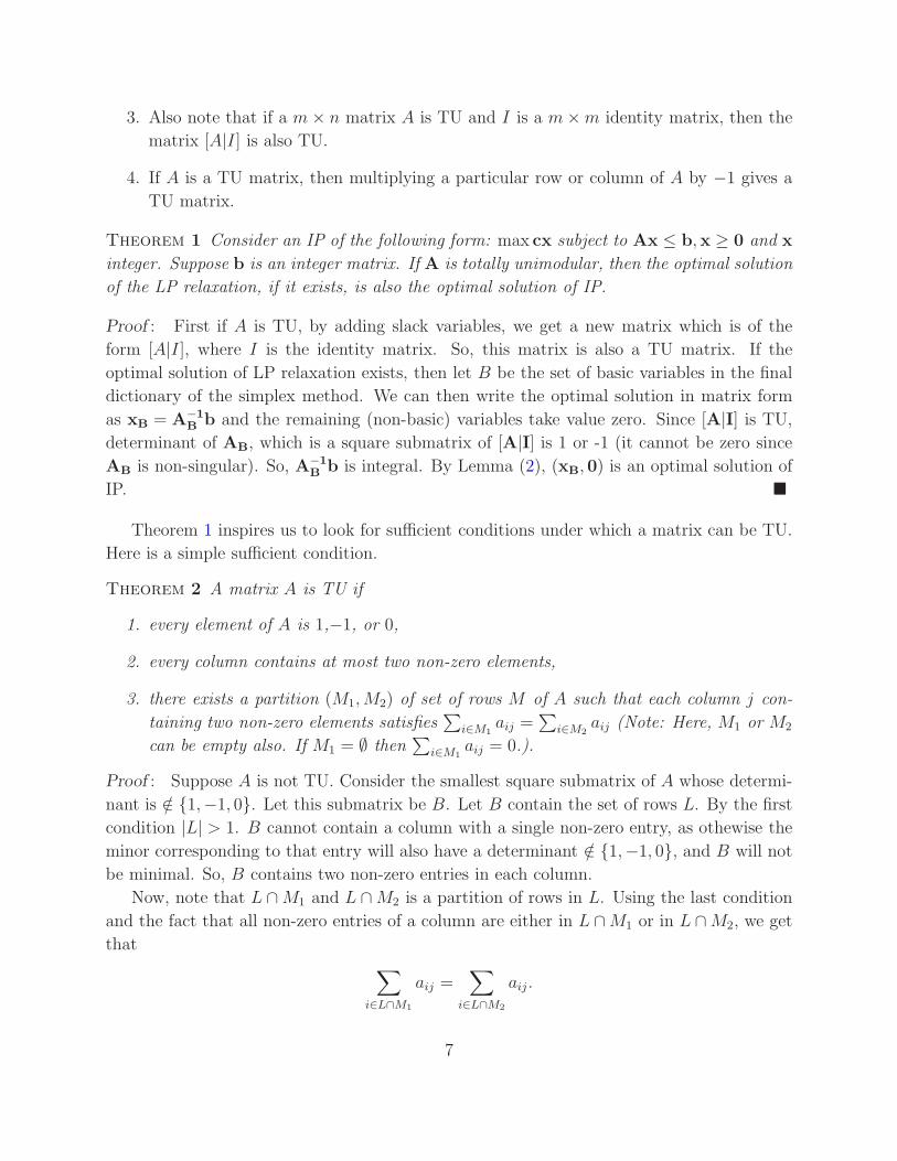
3 Integer Programs with Totally Unimodular Matrices

Definition 3 A matrix A is totally unimodular (TU) if every square submatrix of A

has determinant +1, −1, or 0.

A1 =

1 1 0

−1 1 0

0 0 1

Matrix A1 has a determinant of 2. Hence, it is not TU.

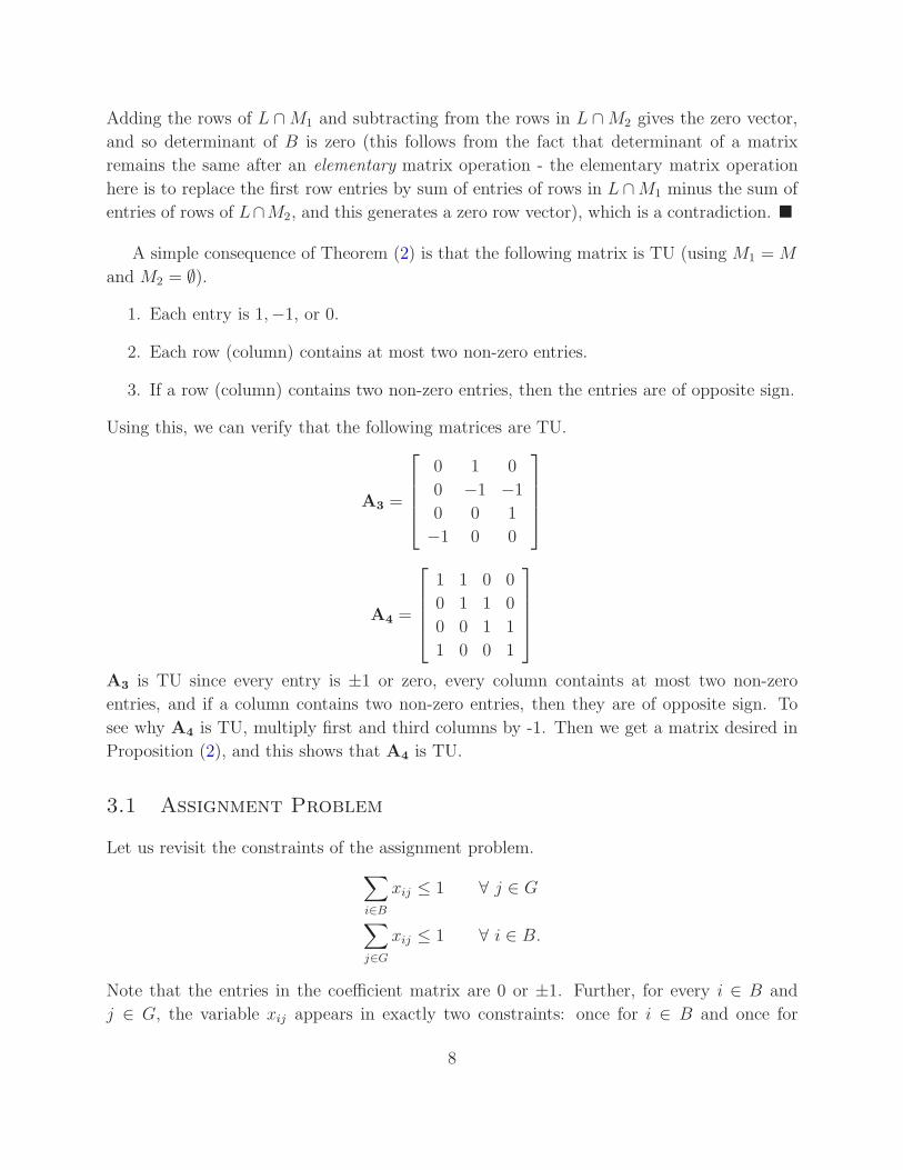
A2 =

1 −1 −1 0

−1 0 0 1

0 1 0 −1

0 0 1 0

However, matrix A2 is TU. Notice some important properties of TU matrices:

1. If A is a TU matrix, then every element of A is either 1, −1, or 0.

2. By the definition of determinant, the transpose of a TU matrix is also TU. Since

transpose of the transpose of a matrix is the same matrix, we can conclude that if the

transpose of a matrix is TU, then so is the original matrix.

6

3. Also note that if a m × n matrix A is TU and I is a m × m identity matrix, then the

matrix [A|I] is also TU.

4. If A is a TU matrix, then multiplying a particular row or column of A by −1 gives a

TU matrix.

Theorem 1 Consider an IP of the following form: max cx subject to Ax ≤ b,x ≥ 0 and x

integer. Suppose b is an integer matrix. If A is totally unimodular, then the optimal solution

of the LP relaxation, if it exists, is also the optimal solution of IP.

Proof : First if A is TU, by adding slack variables, we get a new matrix which is of the

form [A|I], where I is the identity matrix. So, this matrix is also a TU matrix. If the

optimal solution of LP relaxation exists, then let B be the set of basic variables in the final

dictionary of the simplex method. We can then write the optimal solution in matrix form

as xB = A−1

Bb and the remaining (non-basic) variables take value zero. Since [A|I] is TU,

determinant of AB, which is a square submatrix of [A|I] is 1 or -1 (it cannot be zero since

AB is non-singular). So, A−1

Bb is integral. By Lemma (2), (xB, 0) is an optimal solution of

IP.

Theorem 1 inspires us to look for sufficient conditions under which a matrix can be TU.

Here is a simple sufficient condition.

Theorem 2 A matrix A is TU if

1. every element of A is 1,−1, or 0,

2. every column contains at most two non-zero elements,

3. there exists a partition (M1, M2) of set of rows M of A such that each column j con-

taining two non-zero elements satisfies∑

i∈M1aij =

∑

i∈M2aij (Note: Here, M1 or M2

can be empty also. If M1 = ∅ then∑

i∈M1aij = 0.).

Proof : Suppose A is not TU. Consider the smallest square submatrix of A whose determi-

nant is /∈ 1,−1, 0. Let this submatrix be B. Let B contain the set of rows L. By the first

condition |L| > 1. B cannot contain a column with a single non-zero entry, as othewise the

minor corresponding to that entry will also have a determinant /∈ 1,−1, 0, and B will not

be minimal. So, B contains two non-zero entries in each column.

Now, note that L ∩ M1 and L ∩ M2 is a partition of rows in L. Using the last condition

and the fact that all non-zero entries of a column are either in L ∩ M1 or in L ∩ M2, we get

that∑

i∈L∩M1

aij =∑

i∈L∩M2

aij .

7

Adding the rows of L ∩ M1 and subtracting from the rows in L ∩ M2 gives the zero vector,

and so determinant of B is zero (this follows from the fact that determinant of a matrix

remains the same after an elementary matrix operation - the elementary matrix operation

here is to replace the first row entries by sum of entries of rows in L ∩M1 minus the sum of

entries of rows of L∩M2, and this generates a zero row vector), which is a contradiction.

A simple consequence of Theorem (2) is that the following matrix is TU (using M1 = M

and M2 = ∅).

1. Each entry is 1,−1, or 0.

2. Each row (column) contains at most two non-zero entries.

3. If a row (column) contains two non-zero entries, then the entries are of opposite sign.

Using this, we can verify that the following matrices are TU.

A3 =

0 1 0

0 −1 −1

0 0 1

−1 0 0

A4 =

1 1 0 0

0 1 1 0

0 0 1 1

1 0 0 1

A3 is TU since every entry is ±1 or zero, every column containts at most two non-zero

entries, and if a column contains two non-zero entries, then they are of opposite sign. To

see why A4 is TU, multiply first and third columns by -1. Then we get a matrix desired in

Proposition (2), and this shows that A4 is TU.

3.1 Assignment Problem

Let us revisit the constraints of the assignment problem.

∑

i∈B

xij ≤ 1 ∀ j ∈ G

∑

j∈G

xij ≤ 1 ∀ i ∈ B.

Note that the entries in the coefficient matrix are 0 or ±1. Further, for every i ∈ B and

j ∈ G, the variable xij appears in exactly two constraints: once for i ∈ B and once for

8

j ∈ G. Now multiply the entries corresponding to entries of i ∈ B by −1 (note that the

original constraint matrix is TU if and only if this matrix is TU). Now, every column of

the constraint matrix has exactly two non-zero entries and both have opposite signs. This

implies that the constraint matrix is TU. Since the b matrix is a matrix of 1s, we get that

the LP relaxation of the assignment problem IP gives integral solution.

Here is an example which illustrates why the constraint matrix is TU. Suppose there are

two goods and three buyers. Then, there are five constraints.

x11 + x12 ≤ 1

x21 + x22 ≤ 1

x31 + x32 ≤ 1

x11 + x21 + x31 ≤ 1

x12 + x22 + x32 ≤ 1.

The constraint matrix can be written as follows.

A =

1 1 0 0 0 0

0 0 1 1 0 0

0 0 0 0 1 1

1 0 1 0 1 0

0 1 0 1 0 1

Multiplying the last two rows of A by −1, we get A′ as below, and it is clear that it satisfies

the sufficient conditions for being TU.

A′ =

1 1 0 0 0 0

0 0 1 1 0 0

0 0 0 0 1 1

−1 0 −1 0 −1 0

0 −1 0 −1 0 −1

3.2 Potential Constraints are TU

Consider the potential constraints of a weighted digraph G = (N, E, w). It says p : N → R

is a potential if

pj − pi ≤ wij ∀ (i, j) ∈ E.

Now, for every constraint corresponding to (i, j) ∈ E, we have exactly two variables: pi and

pj. The coefficients of these two variables are of opposite sign and are 1 or −1. Hence, the

sufficient conditions for the constraint matrix to be TU are met. This implies that if weights

of this digraph are integers, then any linear optimization over these potentials must give an

integer potential as an optimal solution.

9

3.3 Network Flow Problem

The network flow problem is a classical problem in combinatorial optimization. In this

problem, we are given a digraph G = (N, E). Every edge (i, j) has a capacity hij ≥ 0. Every

node i ∈ N has a supply/demand of bi units of a commodity. If bi > 0, then it is a supply

node, if bi < 0, then it is a demand node, else it is a neutral node. The assumption is total

supply equals total demand:∑

i∈N bi = 0. There is a cost function associated with the edges

of the graph: c : E → R+, where cij denotes the cost of flowing one unit from node i to

node j. The objective is to take the units of commodity from supply node and place it at

the demand nodes with minimum cost.

The decision variable of the problem is xij for all (i, j) ∈ E. The amount xij is called the

flow in edge (i, j). Hence, the objective function is clearly the following.

min∑

(i,j)∈E

cijxij .

For constraints, note that the flow must respect the capacity constraints of edges. Hence,

the following constraint must hold.

0 ≤ xij ≤ hij ∀ (i, j) ∈ E.

Define the nodes on outgoing edges from i as N+(i) = j ∈ N : (i, j) ∈ E and the nodes

on incoming edges from i as N−(i) = j ∈ N : (j, i) ∈ E. Now, consider the following set

of constraints.∑

j∈N+(i)

xij −∑

j∈N−(i)

xji = bi ∀ i ∈ N.

The above constraints are called flow balancing constraints, i.e., the amount of flow out

of a node must equal the flow into a node plus the supply at that node. Note that if we

add all the flow balancing constraints, the left hand side is zero and the right hand side is∑

i∈N bi. Hence, for the problem to be feasible, it is necessary that∑

i∈N bi = 0. Hence, the

minimum cost network flow problem can be formulated as follows.

min∑

(i,j)∈E

cijxij

s.t. (NF)∑

j∈N+(i)

xij −∑

j∈N−(i)

xji = bi ∀ i ∈ N.

0 ≤ xij ≤ hij ∀ (i, j) ∈ E.

Note that (NF) is a linear program. Nevertheless, we show that the constraint matrix

of this problem is TU. To see this, note that the capacity constraint matrix is an identity

10

matrix. Hence, it suffices to show that the flow balancing constraint matrix is TU. To see

this, note that every edge is an incoming edge of a unique node and outgoing edge of a unique

node. Hence, for every (i, j) ∈ E, xij appears exactly in two flow balancing constraints, once

with coefficient 1 and again with coefficient −1. By our earlier result, this matrix is TU. A

consequence of this result is that if the supply (bis) and capacities (hijs) are integral, then

there exists an integral minimum cost network flows.

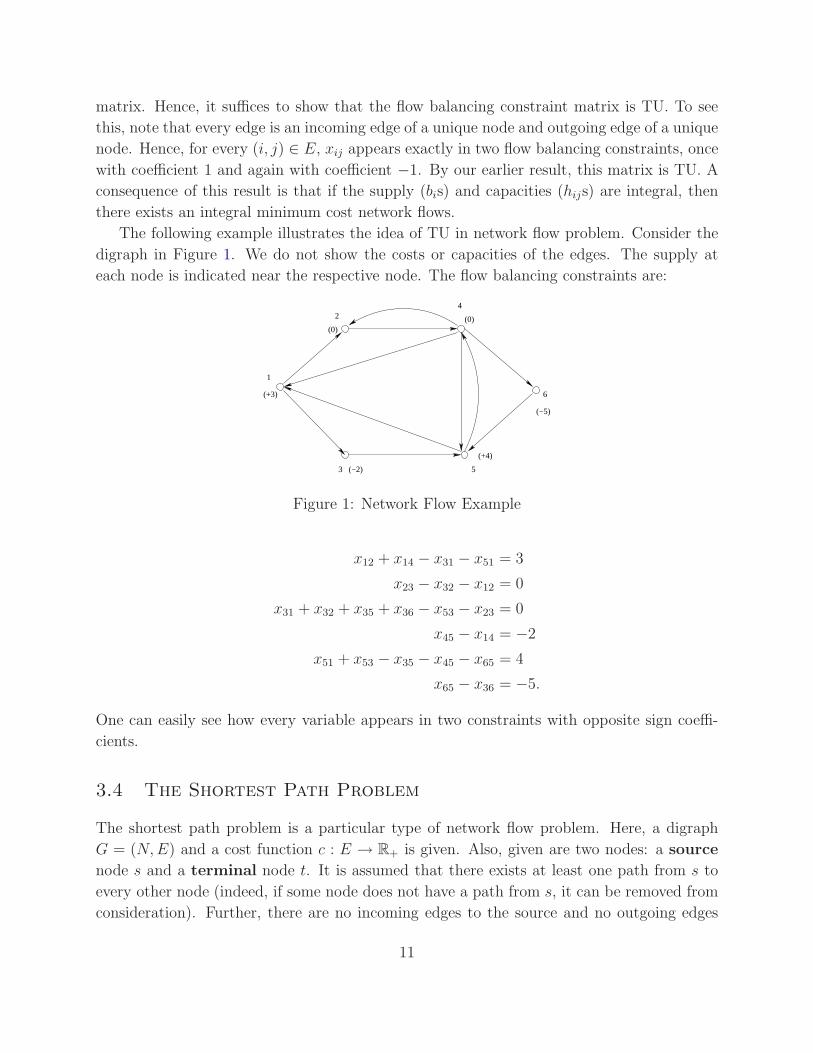
The following example illustrates the idea of TU in network flow problem. Consider the

digraph in Figure 1. We do not show the costs or capacities of the edges. The supply at

each node is indicated near the respective node. The flow balancing constraints are:

1

2

3

4

5

6

(0)(0)

(−5)

(+4)

(−2)

(+3)

Figure 1: Network Flow Example

x12 + x14 − x31 − x51 = 3

x23 − x32 − x12 = 0

x31 + x32 + x35 + x36 − x53 − x23 = 0

x45 − x14 = −2

x51 + x53 − x35 − x45 − x65 = 4

x65 − x36 = −5.

One can easily see how every variable appears in two constraints with opposite sign coeffi-

cients.

3.4 The Shortest Path Problem

The shortest path problem is a particular type of network flow problem. Here, a digraph

G = (N, E) and a cost function c : E → R+ is given. Also, given are two nodes: a source

node s and a terminal node t. It is assumed that there exists at least one path from s to

every other node (indeed, if some node does not have a path from s, it can be removed from

consideration). Further, there are no incoming edges to the source and no outgoing edges

11

from the terminal. The objective is to find the shortest path from s to t, i.e., the path with

the minimum length over all paths from s to t.

To model this as a minimum cost network flow problem, let bi = 1 if i = s, bi = −1 if

i = t, and bi = 0 otherwise. Let hij = 1 for all (i, j) ∈ E. A flow of xij = 1 indicates that

edge (i, j) is chosen. Hence, the formulation for the shortest path problem is as follows.

min∑

(i,j)∈E

cijxij

s.t. (SP)∑

j∈N+(i)

xij = 1 i = s

∑

j∈N+(i)

xij −∑

j∈N−(i)

xji = 0 i /∈ s, t

−∑

j∈N−(i)

xji = −1 i = t

xij ∈ 0, 1 ∀ (i, j) ∈ E

To convince that there is an optimal solution which gives a path from s to t, note that

by the first constraint, there is only one flow from s. For every node which is not s or t,

there is a flow from that node if and only if there is a flow into that node. Finally, by the

last constraint, there is one unit flow into node t. Hence, it describes a path. The other

possibility is that we get a cycle. But deleting the cycle cannot increase costs since costs are

non-negative.

Since the constraint matrix is TU, we can write the relaxation as

0 ≤ xij ≤ 1 ∀ (i, j) ∈ E.

Since the objective is to minimize the total cost of a path from s to t, the xij ≤ 1

constraints are redundant. Another way to see this is to consider the dual of the LP relaxation

of (SP) without the xij ≤ 1 constraints. For this, we write the LP relaxation of (SP) without

12

the xij ≤ 1 constraints first.

min∑

(i,j)∈E

cijxij

s.t. (SP-R)

−∑

j∈N+(i)

xij = −1 i = s

−∑

j∈N+(i)

xij +∑

j∈N−(i)

xji = 0 i /∈ s, t

∑

j∈N−(i)

xji = 1 i = t

xij ≥ 0 ∀ (i, j) ∈ E

The dual of (SP-R) is the following formulation.

max pt − ps (1)

s.t. (DSP)

pj − pi ≤ cij ∀ (i, j) ∈ E.

Note that the constraints in the dual are the potential constraints. We already know a feasible

solution of this exists since there can be no cycles of negative length (we assume costs are

non-negative here). We know that one feasible potential is πs = 0 and πi = shortest path

from s to i for all i 6= s. Hence, πt − πs = shortest path from s to t. But for any potential

p, we know that pt − ps ≤ shortest path from s to t (to prove it, take the shortest path from

s to t and add the potential constaints of the edges in that path). Hence, π describes an

optimal solution. By strong duality, (SP-R) gives the shortest path from s to t.

4 Application: Efficient Assignment with Unit Demand

Consider an economy where the set of agents is denoted by M = 1, . . . , m and consisting

of set of indivisible (not necessarily identical) goods denoted by N = 1, . . . , n. Let vij ≥ 0

be the value of agent i ∈ M to good j ∈ N . Each agent is interested in buying at most one

good.

For clarity of expressions that follow, we add a dummy good 0 to the set of goods. Let

N+ = N ∪ 0. If an agent is not assigned any good, then it is assumed that he assigned

the dummy good 0. Further, a dummy good can be assigned to more than one agent and

the value of each agent for the dummy good is zero.

A feasible assignment of goods to agents is one where every agent is assigned exactly one

good from N+ and every good in N is assigned to no more than one agent from M . An

efficient assignment is one that maximizes the total valuations of the agents.

13

To formulate the problem of finding an efficient assignment as an integer program let

xij = 1 if agent i is assigned good j and zero otherwise.

V = max∑

i∈M

∑

j∈N

vijxij

s.t. (IP)∑

i∈M

xij ≤ 1 ∀ j ∈ N

xi0 +∑

j∈N

xij = 1 ∀ i ∈ M

xij ∈ 0, 1 ∀ i ∈ M, ∀ j ∈ N.

xi0 ≥ 0 and integer ∀ i ∈ M.

Notice that the first two sets of constraints ensure that xij ≤ 1 for all i ∈ M and for

all j ∈ N . The only difference from the constraint matrix of the assignment problem is

the introduction of xi0 variables, whose coefficients form an identity matrix. Hence, the

constraints matrix of this formulation is also TU. Hence, the LP relaxation of IP gives

integral solution. Note here that the LP relaxation of xij ∈ 0, 1 is 0 ≤ xij ≤ 1, but the

constraints xij ≤ 1 are redundant here. So, we can write formulation (IP) as the following

linear program:

V = max∑

i∈M

∑

j∈N

vijxij

s.t. (LP)∑

i∈M

xij ≤ 1 ∀ j ∈ N

xi0 +∑

j∈N

xij = 1 ∀ i ∈ M

xi0, xij ≥ 0 ∀ i ∈ M, ∀ j ∈ N.

Now, consider the dual of (LP). For that, we associate with constraint corresponding to agent

i ∈ M a dual variable πi and with constraint corresponding to good j ∈ N a dual variable

pj. The pj variables are non-negative since the corresponding constraints are inequality but

14

πi variables are free.

min∑

i∈M

πi +∑

j∈N

pj

s.t. (DP)

πi + pj ≥ vij ∀ i ∈ M, ∀ j ∈ N

πi ≥ 0 ∀ i ∈ M

pj ≥ 0 ∀ i ∈ M, ∀ j ∈ N.

Note here that even though the πi variables are free, when we write the constraint cor-

responding to variable xi0, it turns out that we recover the non-negativity constraints. The

dual has interesting economic interpretation. pjj∈M can be thought as a price vector on

goods. Given the price vector p, πi ≥ maxj∈N [vij − pj ] for every i ∈ M . If we set p0 = 0,

then vi0 − p0 = 0 implies that πi ≥ 0 can be folded into πi ≥ maxj∈N+ [vij − pj ].

Given any price vector p ∈ R|N+|+ (i.e., on set of goods, including the dummy good), with

p0 = 0, define demand set of buyer i at this price vector p as

Di(p) = j ∈ N+ : vij − pj ≥ vik − pk ∀ k ∈ N+.

Definition 4 A tuple (p, x) is a Walrasian equilibrium, where p is a price vector and x is

a feasible allocation (i.e., a feasible solution to LP), if

1. xij = 1 implies that j ∈ Di(p) (every buyer is assigned a good from his demand set)

and

2.∑

i∈M xij = 0 implies that pj = 0 (unassigned good has zero price).

Given a price vector p (with p0 = 0), we can construct a dual feasible solution from this

p. This is done by setting πi = maxj∈N+[vij − pj ]. Clearly, this (p, π) is a feasible solution

of (DP) - to be exact, we consider price vector p without the dummy good component here

since there is no dual variable corresponding to dummy good. This is because πi ≥ vij − pj

for all i ∈ M and for all j ∈ N . Further πi ≥ vi0 − p0 = 0 for all i ∈ M . From now

on, whenever we say that p is a dual feasible solution, we imply that the corresponding π

variables are defined as above.

Theorem 3 Let p be a feasible solution of (DP) and x be a feasible solution of (LP). (p, x)

is a Walrasian equilibrium if and only if p and x are optimal solutions of (DP) and (LP)

respectively.

15

Proof : Suppose (p, x) is a Walrasian equilibrium. Define πi = maxj∈N+[vij − pj ] for all

i ∈ M . As argued earlier, (p, π) is a feasible solution of (DP). Now, Walrasian equilibrium

conditions can be written as

[πi − (vij − pj)]xij = 0 ∀ i ∈ M, ∀ j ∈ N+

[1 −∑

i∈M

xij ]pj = 0 ∀ j ∈ N.

The first condition comes from the fact that if xij = 1 then j ∈ Di(p), which implies that

πi = vij − pj ≥ vik − pk for all k ∈ N+. The second condition comes from the fact that

unassigned goods must have zero price. Now, the CS conditions of the primal and dual

problems are

[πi − (vij − pj)]xij = 0 ∀ i ∈ M, ∀ j ∈ N

πixi0 = 0 ∀ i ∈ M

[1 −∑

i∈M

xij ]pj = 0 ∀ j ∈ N.

We can fold the second CS condition into first since p0 = 0 and vi0 = 0 for all i ∈ M . This

gives the CS conditions as

[πi − (vij − pj)]xij = 0 ∀ i ∈ M, ∀ j ∈ N+

[1 −∑

i∈M

xij ]pj = 0 ∀ j ∈ N.

Hence, (p, x) satisfies the CS conditions. So, p is an optimal solution of (DP) and x is an

optimal solution of (LP).

The other direction of the proof also follows similarly from the equivalence between the

CS conditions and the Walrasian equilibrium conditions.

5 Branch and Bound Technique to Solve Integer Programs

There is no elegant algorithm (like the simplex algorithm for linear programming) to solve

integer programs. The common method to solve an integer program is enumeration but in a

smart manner. We discuss one such popular enumeration technique called the branch and

bound technique.

The basic idea behind the branch and bound technique is to divide the original integer

program into subproblems. Consider the integer program denoted by max cx subject to

x ∈ S, where S is the feasible region. Let z = maxcx : x ∈ S. The following observation

is crucial.

16

Proposition 1 Let S = S1 ∪ S2 ∪ . . . Sk be a decomposition of S into smaller sets, and let

zi = maxcx : x ∈ Si for every i ∈ 1, . . . , k. Then z = maxi zi.

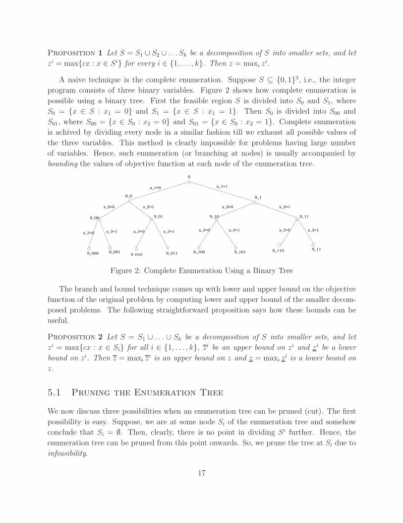
A naive technique is the complete enumeration. Suppose S ⊆ 0, 13, i.e., the integer

program consists of three binary variables. Figure 2 shows how complete enumeration is

possible using a binary tree. First the feasible region S is divided into S0 and S1, where

S0 = x ∈ S : x1 = 0 and S1 = x ∈ S : x1 = 1. Then S0 is divided into S00 and

S01, where S00 = x ∈ S0 : x2 = 0 and S01 = x ∈ S0 : x2 = 1. Complete enumeration

is achived by dividing every node in a similar fashion till we exhaust all possible values of

the three variables. This method is clearly impossible for problems having large number

of variables. Hence, such enumeration (or branching at nodes) is usually accompanied by

bounding the values of objective function at each node of the enumeration tree.

x_2=0

x_3=0 x_3=1

x_2=1

x_3=1x_3=0x_3=1x_3=0x_3=1x_3=0

x_2=0 x_2=1

x_1=0 x_1=1

S

S_0 S_1

S_10 S_11

S_110 S_111S_100 S_101

S_01

S_010 S_011S_000 S_001

S_00

Figure 2: Complete Enumeration Using a Binary Tree

The branch and bound technique comes up with lower and upper bound on the objective

function of the original problem by computing lower and upper bound of the smaller decom-

posed problems. The following straightforward proposition says how these bounds can be

useful.

Proposition 2 Let S = S1 ∪ . . . ∪ Sk be a decomposition of S into smaller sets, and let

zi = maxcx : x ∈ Si for all i ∈ 1, . . . , k, zi be an upper bound on zi and zi be a lower

bound on zi. Then z = maxi zi is an upper bound on z and z = maxi z

i is a lower bound on

z.

5.1 Pruning the Enumeration Tree

We now discuss three possibilities when an enumeration tree can be pruned (cut). The first

possibility is easy. Suppose, we are at some node Si of the enumeration tree and somehow

conclude that Si = ∅. Then, clearly, there is no point in dividing Si further. Hence, the

enumeration tree can be pruned from this point onwards. So, we prune the tree at Si due to

infeasibility.

17

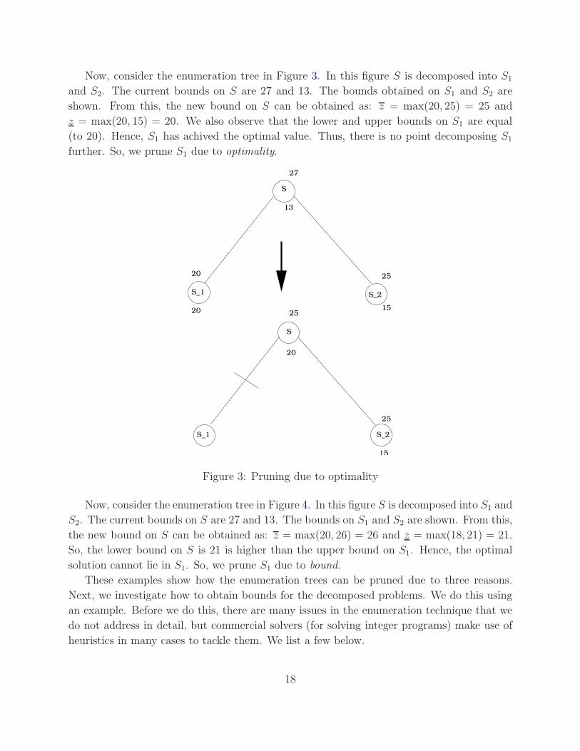
Now, consider the enumeration tree in Figure 3. In this figure S is decomposed into S1

and S2. The current bounds on S are 27 and 13. The bounds obtained on S1 and S2 are

shown. From this, the new bound on S can be obtained as: z = max(20, 25) = 25 and

z = max(20, 15) = 20. We also observe that the lower and upper bounds on S1 are equal

(to 20). Hence, S1 has achived the optimal value. Thus, there is no point decomposing S1

further. So, we prune S1 due to optimality.

S

20

20

25

15

27

13

S_2

S

25

25

20

S_1

S_1

S_2

15

Figure 3: Pruning due to optimality

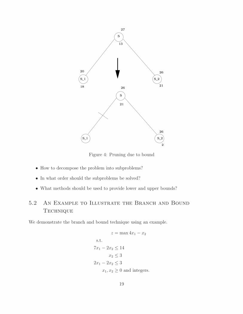
Now, consider the enumeration tree in Figure 4. In this figure S is decomposed into S1 and

S2. The current bounds on S are 27 and 13. The bounds on S1 and S2 are shown. From this,

the new bound on S can be obtained as: z = max(20, 26) = 26 and z = max(18, 21) = 21.

So, the lower bound on S is 21 is higher than the upper bound on S1. Hence, the optimal

solution cannot lie in S1. So, we prune S1 due to bound.

These examples show how the enumeration trees can be pruned due to three reasons.

Next, we investigate how to obtain bounds for the decomposed problems. We do this using

an example. Before we do this, there are many issues in the enumeration technique that we

do not address in detail, but commercial solvers (for solving integer programs) make use of

heuristics in many cases to tackle them. We list a few below.

18

S

20

27

13

S_2

S

18

26

2126

21

26

21

S_1 S_2

S_1

Figure 4: Pruning due to bound

• How to decompose the problem into subproblems?

• In what order should the subproblems be solved?

• What methods should be used to provide lower and upper bounds?

5.2 An Example to Illustrate the Branch and Bound

Technique

We demonstrate the branch and bound technique using an example.

z = max 4x1 − x2

s.t.

7x1 − 2x2 ≤ 14

x2 ≤ 3

2x1 − 2x2 ≤ 3

x1, x2 ≥ 0 and integers.

19

Bounding: To obtain the first upper bound, we solve the LP relaxation of this problem.

The optimal solution of the LP relaxation is 597

with (x1, x2) = (207, 3). Hence, z = 59

7. There

is no formal way to get a feasible solution. So, we do not have a lower bound, and set

z = −∞.

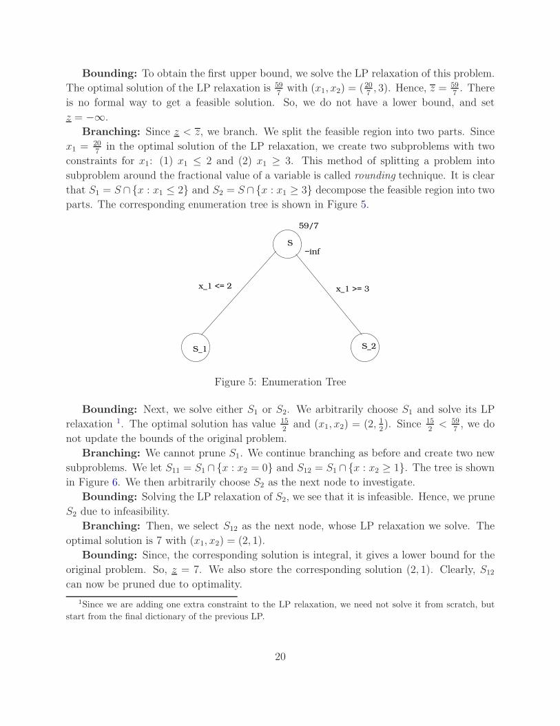
Branching: Since z < z, we branch. We split the feasible region into two parts. Since

x1 = 207

in the optimal solution of the LP relaxation, we create two subproblems with two

constraints for x1: (1) x1 ≤ 2 and (2) x1 ≥ 3. This method of splitting a problem into

subproblem around the fractional value of a variable is called rounding technique. It is clear

that S1 = S ∩x : x1 ≤ 2 and S2 = S ∩x : x1 ≥ 3 decompose the feasible region into two

parts. The corresponding enumeration tree is shown in Figure 5.

S

S_1 S_2

59/7

−inf

x_1 >= 3x_1 <= 2

Figure 5: Enumeration Tree

Bounding: Next, we solve either S1 or S2. We arbitrarily choose S1 and solve its LP

relaxation 1. The optimal solution has value 152

and (x1, x2) = (2, 12). Since 15

2< 59

7, we do

not update the bounds of the original problem.

Branching: We cannot prune S1. We continue branching as before and create two new

subproblems. We let S11 = S1 ∩x : x2 = 0 and S12 = S1 ∩x : x2 ≥ 1. The tree is shown

in Figure 6. We then arbitrarily choose S2 as the next node to investigate.

Bounding: Solving the LP relaxation of S2, we see that it is infeasible. Hence, we prune

S2 due to infeasibility.

Branching: Then, we select S12 as the next node, whose LP relaxation we solve. The

optimal solution is 7 with (x1, x2) = (2, 1).

Bounding: Since, the corresponding solution is integral, it gives a lower bound for the

original problem. So, z = 7. We also store the corresponding solution (2, 1). Clearly, S12

can now be pruned due to optimality.

1Since we are adding one extra constraint to the LP relaxation, we need not solve it from scratch, but

start from the final dictionary of the previous LP.

20

S

S_1 S_2

59/7

−inf

x_1 >= 3

S_11 S_12

x_2 >= 1x_2=0

15/2

x_1 <= 2

Figure 6: Enumeration Tree

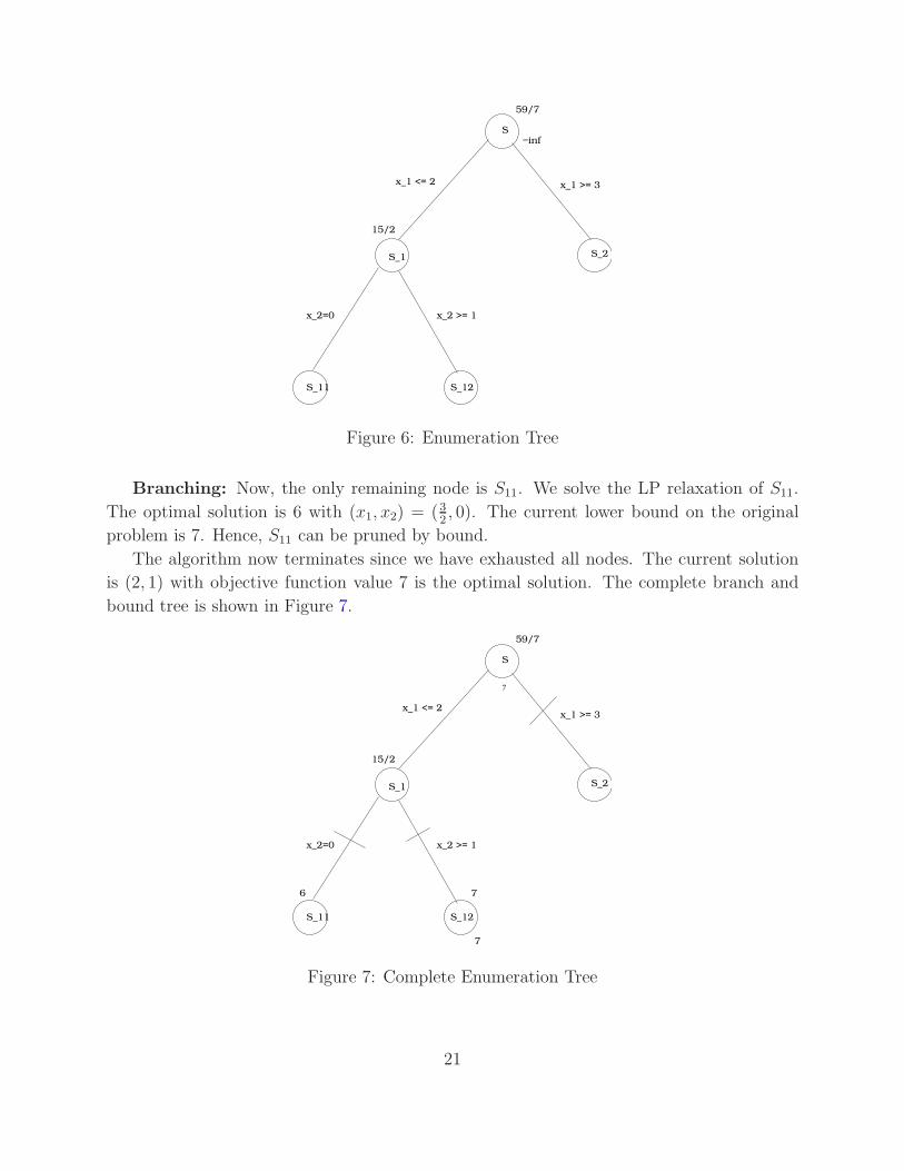
Branching: Now, the only remaining node is S11. We solve the LP relaxation of S11.

The optimal solution is 6 with (x1, x2) = (32, 0). The current lower bound on the original

problem is 7. Hence, S11 can be pruned by bound.

The algorithm now terminates since we have exhausted all nodes. The current solution

is (2, 1) with objective function value 7 is the optimal solution. The complete branch and

bound tree is shown in Figure 7.

S

S_2

59/7

x_1 >= 3

7

x_1 <= 2

x_2=0 x_2 >= 1

S_11 S_12

S_1

6 7

7

15/2

Figure 7: Complete Enumeration Tree

21

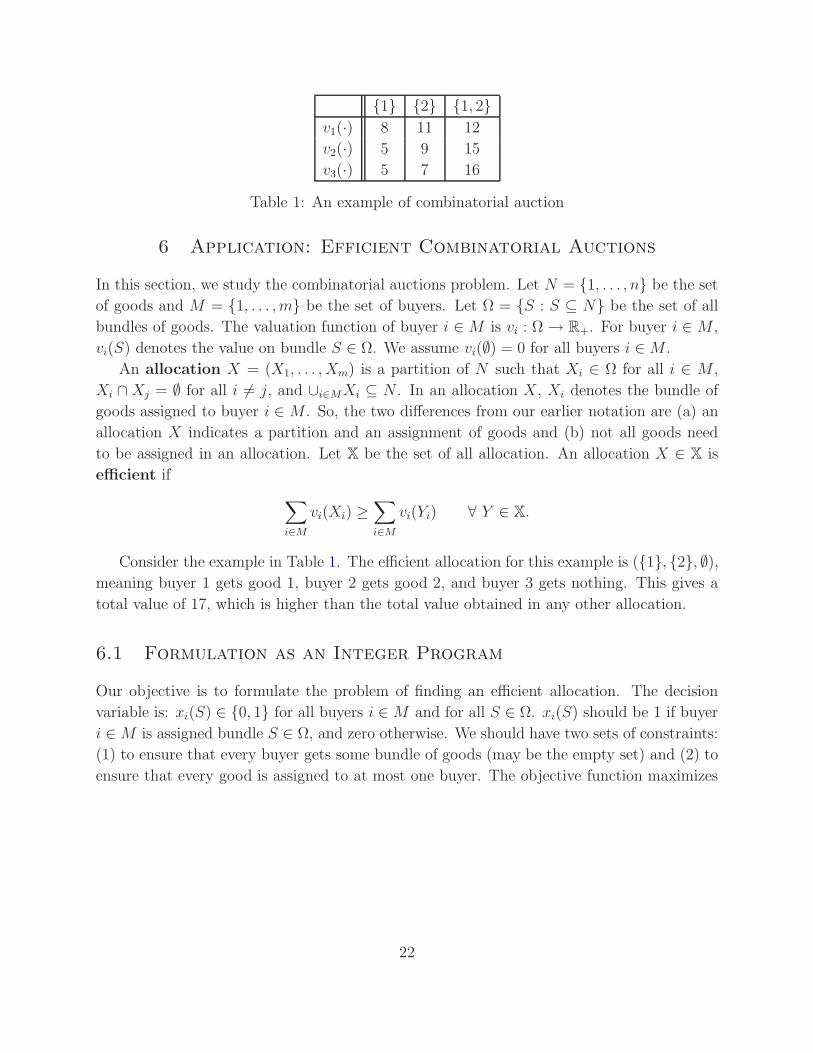
1 2 1, 2

v1(·) 8 11 12

v2(·) 5 9 15

v3(·) 5 7 16

Table 1: An example of combinatorial auction

6 Application: Efficient Combinatorial Auctions

In this section, we study the combinatorial auctions problem. Let N = 1, . . . , n be the set

of goods and M = 1, . . . , m be the set of buyers. Let Ω = S : S ⊆ N be the set of all

bundles of goods. The valuation function of buyer i ∈ M is vi : Ω → R+. For buyer i ∈ M ,

vi(S) denotes the value on bundle S ∈ Ω. We assume vi(∅) = 0 for all buyers i ∈ M .

An allocation X = (X1, . . . , Xm) is a partition of N such that Xi ∈ Ω for all i ∈ M ,

Xi ∩ Xj = ∅ for all i 6= j, and ∪i∈MXi ⊆ N . In an allocation X, Xi denotes the bundle of

goods assigned to buyer i ∈ M . So, the two differences from our earlier notation are (a) an

allocation X indicates a partition and an assignment of goods and (b) not all goods need

to be assigned in an allocation. Let X be the set of all allocation. An allocation X ∈ X is

efficient if

∑

i∈M

vi(Xi) ≥∑

i∈M

vi(Yi) ∀ Y ∈ X.

Consider the example in Table 1. The efficient allocation for this example is (1, 2, ∅),

meaning buyer 1 gets good 1, buyer 2 gets good 2, and buyer 3 gets nothing. This gives a

total value of 17, which is higher than the total value obtained in any other allocation.

6.1 Formulation as an Integer Program

Our objective is to formulate the problem of finding an efficient allocation. The decision

variable is: xi(S) ∈ 0, 1 for all buyers i ∈ M and for all S ∈ Ω. xi(S) should be 1 if buyer

i ∈ M is assigned bundle S ∈ Ω, and zero otherwise. We should have two sets of constraints:

(1) to ensure that every buyer gets some bundle of goods (may be the empty set) and (2) to

ensure that every good is assigned to at most one buyer. The objective function maximizes

22

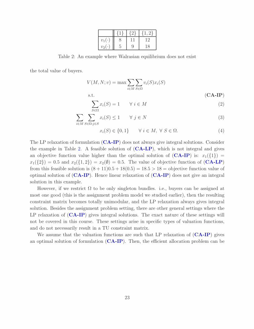
1 2 1, 2

v1(·) 8 11 12

v2(·) 5 9 18

Table 2: An example where Walrasian equilibrium does not exist

the total value of buyers.

V (M, N ; v) = max∑

i∈M

∑

S∈Ω

vi(S)xi(S)

s.t. (CA-IP)∑

S∈Ω

xi(S) = 1 ∀ i ∈ M (2)

∑

i∈M

∑

S∈Ω:j∈S

xi(S) ≤ 1 ∀ j ∈ N (3)

xi(S) ∈ 0, 1 ∀ i ∈ M, ∀ S ∈ Ω. (4)

The LP relaxation of formulation (CA-IP) does not always give integral solutions. Consider

the example in Table 2. A feasible solution of (CA-LP), which is not integral and gives

an objective function value higher than the optimal solution of (CA-IP) is: x1(1) =

x1(2) = 0.5 and x2(1, 2) = x2(∅) = 0.5. The value of objective function of (CA-LP)

from this feasible solution is (8 + 11)0.5 + 18(0.5) = 18.5 > 18 = objective function value of

optimal solution of (CA-IP). Hence linear relaxation of (CA-IP) does not give an integral

solution in this example.

However, if we restrict Ω to be only singleton bundles. i.e., buyers can be assigned at

most one good (this is the assignment problem model we studied earlier), then the resulting

constraint matrix becomes totally unimodular, and the LP relaxation always gives integral

solution. Besides the assignment problem setting, there are other general settings where the

LP relaxation of (CA-IP) gives integral solutions. The exact nature of these settings will

not be covered in this course. These settings arise in specific types of valuation functions,

and do not necessarily result in a TU constraint matrix.

We assume that the valuation functions are such that LP relaxation of (CA-IP) gives

an optimal solution of formulation (CA-IP). Then, the efficient allocation problem can be

23

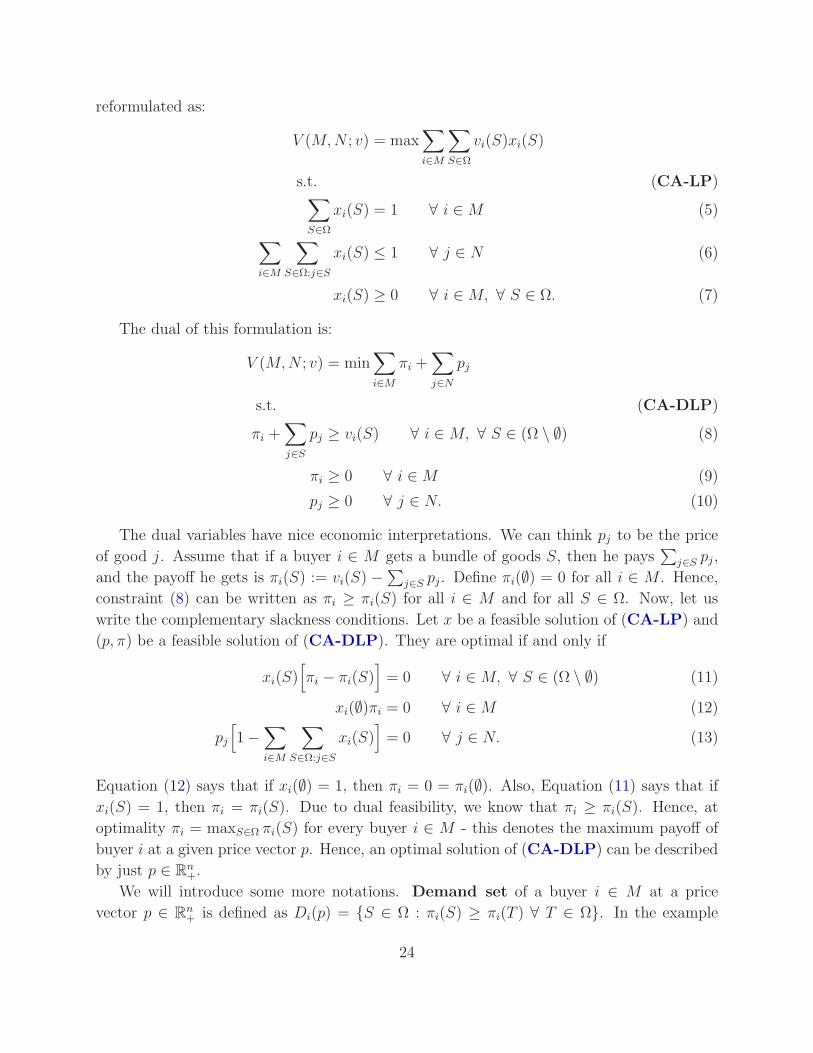
reformulated as:

V (M, N ; v) = max∑

i∈M

∑

S∈Ω

vi(S)xi(S)

s.t. (CA-LP)∑

S∈Ω

xi(S) = 1 ∀ i ∈ M (5)

∑

i∈M

∑

S∈Ω:j∈S

xi(S) ≤ 1 ∀ j ∈ N (6)

xi(S) ≥ 0 ∀ i ∈ M, ∀ S ∈ Ω. (7)

The dual of this formulation is:

V (M, N ; v) = min∑

i∈M

πi +∑

j∈N

pj

s.t. (CA-DLP)

πi +∑

j∈S

pj ≥ vi(S) ∀ i ∈ M, ∀ S ∈ (Ω \ ∅) (8)

πi ≥ 0 ∀ i ∈ M (9)

pj ≥ 0 ∀ j ∈ N. (10)

The dual variables have nice economic interpretations. We can think pj to be the price

of good j. Assume that if a buyer i ∈ M gets a bundle of goods S, then he pays∑

j∈S pj,

and the payoff he gets is πi(S) := vi(S) −∑

j∈S pj . Define πi(∅) = 0 for all i ∈ M . Hence,

constraint (8) can be written as πi ≥ πi(S) for all i ∈ M and for all S ∈ Ω. Now, let us

write the complementary slackness conditions. Let x be a feasible solution of (CA-LP) and

(p, π) be a feasible solution of (CA-DLP). They are optimal if and only if

xi(S)[

πi − πi(S)]

= 0 ∀ i ∈ M, ∀ S ∈ (Ω \ ∅) (11)

xi(∅)πi = 0 ∀ i ∈ M (12)

pj

[

1 −∑

i∈M

∑

S∈Ω:j∈S

xi(S)]

= 0 ∀ j ∈ N. (13)

Equation (12) says that if xi(∅) = 1, then πi = 0 = πi(∅). Also, Equation (11) says that if

xi(S) = 1, then πi = πi(S). Due to dual feasibility, we know that πi ≥ πi(S). Hence, at

optimality πi = maxS∈Ω πi(S) for every buyer i ∈ M - this denotes the maximum payoff of

buyer i at a given price vector p. Hence, an optimal solution of (CA-DLP) can be described

by just p ∈ Rn+.

We will introduce some more notations. Demand set of a buyer i ∈ M at a price

vector p ∈ Rn+ is defined as Di(p) = S ∈ Ω : πi(S) ≥ πi(T ) ∀ T ∈ Ω. In the example

24

above, consider a price vector p = (4, 4) (i.e., price of good 1 is 4, good 2 is 4, and bundle

1,2 is 4+4=8). At this price vector, D1(p) = 1, 1, 2, D2(p) = 2, and D3(p) =

1, 2. Consider another price vector p′ = (7, 8). At this price vector, D1(p′) = 1,

D2(p′) = 2, and D3(p

′) = ∅, 1.

Definition 5 A price vector p ∈ Rn+ and an allocation X is called a Walrasian equilib-

rium if

1. Xi ∈ Di(p) for all i ∈ M (every buyer gets a bundle with maximum payoff),

2. pj = 0 for all j ∈ N such that j /∈ ∪i∈MXi (unassigned goods have zero price).

The price vector p′ = (7, 8) along with allocation (1, 2, ∅) is a Walrasian equilibrium of

the previous example since 1 ∈ D1(p′), 2 ∈ D2(p

′), and ∅ ∈ D3(p′).

Theorem 4 (p, X) is a Walrasian equilibrium if and only if X corresponds to an optimal

solution of (CA-LP) and p corresponds to an optimal solution of (CA-DLP).

Proof : Suppose (p, X) is a Walrasian equilibrium. Then p generates a feasible solution of

(CA-DLP) - this feasible solution is generated by setting πi = maxS∈Ω[vi(S)−∑

j∈S pj] for

all i ∈ M , and X corresponds to a feasible solution of (CA-LP) - this feasible solution is

generated by setting xi(Xi) = 1 for all i ∈ M and setting zero all other x variables. Now,

Xi ∈ Di(p) for all i ∈ M implies that πi = πi(Xi) for all i ∈ M , and this further implies that

Equations (11) and (12) is satisfied. Similarly, pj = 0 for all j ∈ N that are not assigned

in X. This means Equation (13) is satisfied. Since complementary slackness conditions are

satisfied, these are also optimal solutions.

Now, suppose p is an optimal solution of (CA-DLP) and X corresponds to an optimal

solution of (CA-LP). Then, the complementary slackness conditions imply that the condi-

tions for Walrasian equilibrium is satisfied. Hence, (p, X) is a Walrasian equilibrium.

Another way to state Theorem 4 is that a Walrasian equilibrium exists if and only if an

optimal solution of (CA-LP) gives an efficient allocation (an optimal solution of (CA-IP).

This is because if a Walrasian equilibrium (p, X) exists, then X is an optimal solution

of (CA-LP) that is integral. Hence it is an optimal solution of (CA-IP) or an efficient

allocation. So, every allocation corresponding to a Walrasian equilibrium is an efficient

allocation.

There are combinatorial auction problems where a Walrasian equilibrium may not exist.

Consider the example in Table 2. It can be verified that this example does not have a

Walrasian equilibrium. Suppose there is a Walrasian equilibrium (p, X). By Theorem 4 and

the earlier discussion, X is efficient, i.e, X = (∅, 1, 2). Since X1 = ∅, by definition of

Walrasian equilibrium π1(∅) = 0 ≥ π1(1) = 8 − p1, i.e., p1 ≥ 8. Similarly, p2 ≥ 11. This

25

means p1 + p2 ≥ 19. But X2 = 1, 2, and π2(1, 2) = 18 − (p1 + p2) ≤ −1 < 0 = π2(∅).

Hence 1, 2 /∈ D2(p). This is a contradiction since (p, X) is a Walrasian equilibrium. This

also follows from the fact the LP relaxation of (CA-IP) does not have integral optimal

solution.

26