Embed Size (px)
Citation preview


ii
Abstract
Reversible integer-to-integer (ITI) wavelet transforms are studied in the context of image coding. Considered arematters such as transform frameworks, transform design techniques, the utility of transforms for image coding, andnumerous practical issues related to transforms.
The generalized reversible ITI transform (GRITIT) framework, a single unified framework for reversible ITIwavelet/block transforms, is proposed. This new framework is then used to study several previously proposed frame-works and their interrelationships. For example, the framework based on the overlapping rounding transform is shownto be a special case of the lifting framework with only trivial extensions. The applicability of the GRITIT frameworkfor block transforms is also demonstrated. Throughout all of this work, particularly close attention is paid to roundingoperators and their characteristics.
Strategies for handling the transformation of arbitrary-length signals in a nonexpansive manner are considered(e.g., symmetric extension, per-displace-step extension). Two families of symmetry-preserving transforms (which arecompatible with symmetric extension) are introduced and studied. We characterize transforms belonging to thesefamilies. Some new reversible ITI structures that are useful for constructing symmetry-preserving transforms arealso proposed. A simple search-based design technique is explored as means for finding effective low-complexitytransforms in the above-mentioned families.
In the context of image coding, a number of reversible ITI wavelet transforms are compared on the basis of theirlossy compression performance, lossless compression performance, and computational complexity. Of the transformsconsidered, several were found to perform particularly well, with the best choice for a given application depending onthe relative importance of the preceding criteria. Reversible ITI versions of numerous transforms are also comparedto their conventional (i.e., non-reversible real-to-real) counterparts for lossy compression. At low bit rates, reversibleITI and conventional versions of transforms were found to often yield results of comparable quality. Factors affectingthe compression performance of reversible ITI wavelet transforms are also presented, supported by both experimentaldata and theoretical arguments.
In addition to this work, the JPEG-2000 image compression standard is discussed. In particular, the JPEG-2000Part-1 codec is described, analyzed, and evaluated.
iii
Contents
Abstract . . . . . . . . . . . . . . . . . . . . . . . . . . . . . . . . . . . . . . . . . . . . . . . . . . . . . . . ii
Contents . . . . . . . . . . . . . . . . . . . . . . . . . . . . . . . . . . . . . . . . . . . . . . . . . . . . . . iii
List of Tables . . . . . . . . . . . . . . . . . . . . . . . . . . . . . . . . . . . . . . . . . . . . . . . . . . . . vii
List of Figures . . . . . . . . . . . . . . . . . . . . . . . . . . . . . . . . . . . . . . . . . . . . . . . . . . . viii
List of Algorithms . . . . . . . . . . . . . . . . . . . . . . . . . . . . . . . . . . . . . . . . . . . . . . . . . x
List of Acronyms . . . . . . . . . . . . . . . . . . . . . . . . . . . . . . . . . . . . . . . . . . . . . . . . . . xi
Preface . . . . . . . . . . . . . . . . . . . . . . . . . . . . . . . . . . . . . . . . . . . . . . . . . . . . . . . xiiiAcknowledgments . . . . . . . . . . . . . . . . . . . . . . . . . . . . . . . . . . . . . . . . . . . . . . . . xiiiDedication . . . . . . . . . . . . . . . . . . . . . . . . . . . . . . . . . . . . . . . . . . . . . . . . . . . . xv
1 Introduction . . . . . . . . . . . . . . . . . . . . . . . . . . . . . . . . . . . . . . . . . . . . . . . . . . 11.1 Reversible Integer-to-Integer (ITI) Wavelet Transforms . . . . . . . . . . . . . . . . . . . . . . . . . 11.2 Utility of Reversible ITI Wavelet Transforms . . . . . . . . . . . . . . . . . . . . . . . . . . . . . . 11.3 Common Misconceptions . . . . . . . . . . . . . . . . . . . . . . . . . . . . . . . . . . . . . . . . . 21.4 Historical Perspective . . . . . . . . . . . . . . . . . . . . . . . . . . . . . . . . . . . . . . . . . . . 21.5 Overview and Contribution of the Thesis . . . . . . . . . . . . . . . . . . . . . . . . . . . . . . . . . 4
2 Preliminaries . . . . . . . . . . . . . . . . . . . . . . . . . . . . . . . . . . . . . . . . . . . . . . . . . . 62.1 Introduction . . . . . . . . . . . . . . . . . . . . . . . . . . . . . . . . . . . . . . . . . . . . . . . . 62.2 Notation and Terminology . . . . . . . . . . . . . . . . . . . . . . . . . . . . . . . . . . . . . . . . 62.3 Multirate Filter Banks and Wavelet Systems . . . . . . . . . . . . . . . . . . . . . . . . . . . . . . . 8
2.3.1 Multirate Systems . . . . . . . . . . . . . . . . . . . . . . . . . . . . . . . . . . . . . . . . 92.3.2 Sampling . . . . . . . . . . . . . . . . . . . . . . . . . . . . . . . . . . . . . . . . . . . . . 92.3.3 Downsampling . . . . . . . . . . . . . . . . . . . . . . . . . . . . . . . . . . . . . . . . . . 92.3.4 Upsampling . . . . . . . . . . . . . . . . . . . . . . . . . . . . . . . . . . . . . . . . . . . . 112.3.5 Noble Identities . . . . . . . . . . . . . . . . . . . . . . . . . . . . . . . . . . . . . . . . . . 112.3.6 Polyphase Representation of Signals and Filters . . . . . . . . . . . . . . . . . . . . . . . . . 112.3.7 Filter Banks . . . . . . . . . . . . . . . . . . . . . . . . . . . . . . . . . . . . . . . . . . . . 132.3.8 Uniformly Maximally-Decimated (UMD) Filter Banks . . . . . . . . . . . . . . . . . . . . . 132.3.9 Perfect-Reconstruction (PR) UMD Filter Banks . . . . . . . . . . . . . . . . . . . . . . . . . 132.3.10 Polyphase Form of a UMD Filter Bank . . . . . . . . . . . . . . . . . . . . . . . . . . . . . 142.3.11 Conditions for PR System . . . . . . . . . . . . . . . . . . . . . . . . . . . . . . . . . . . . 162.3.12 Octave-Band Filter Banks . . . . . . . . . . . . . . . . . . . . . . . . . . . . . . . . . . . . 162.3.13 UMD Filter Bank Implementation . . . . . . . . . . . . . . . . . . . . . . . . . . . . . . . . 17
2.4 Image Coding . . . . . . . . . . . . . . . . . . . . . . . . . . . . . . . . . . . . . . . . . . . . . . . 172.4.1 Image Coding and Compression . . . . . . . . . . . . . . . . . . . . . . . . . . . . . . . . . 172.4.2 Transform-Based Image Compression Systems . . . . . . . . . . . . . . . . . . . . . . . . . 182.4.3 Wavelet Transforms for Image Compression . . . . . . . . . . . . . . . . . . . . . . . . . . . 192.4.4 Compression Performance Measures . . . . . . . . . . . . . . . . . . . . . . . . . . . . . . . 19
Contents iv
3 Frameworks for Reversible ITI Wavelet/Block Transforms . . . . . . . . . . . . . . . . . . . . . . . . 213.1 Introduction . . . . . . . . . . . . . . . . . . . . . . . . . . . . . . . . . . . . . . . . . . . . . . . . 213.2 Rounding Operators . . . . . . . . . . . . . . . . . . . . . . . . . . . . . . . . . . . . . . . . . . . . 22
3.2.1 Integer-Bias Invariance and Oddness . . . . . . . . . . . . . . . . . . . . . . . . . . . . . . . 223.2.2 Relationships Involving Rounding Functions . . . . . . . . . . . . . . . . . . . . . . . . . . 233.2.3 Rounding Error . . . . . . . . . . . . . . . . . . . . . . . . . . . . . . . . . . . . . . . . . . 25
3.3 Previously Proposed Frameworks . . . . . . . . . . . . . . . . . . . . . . . . . . . . . . . . . . . . . 283.3.1 S Transform . . . . . . . . . . . . . . . . . . . . . . . . . . . . . . . . . . . . . . . . . . . . 283.3.2 S+P Transform Framework . . . . . . . . . . . . . . . . . . . . . . . . . . . . . . . . . . . . 293.3.3 Lifting Framework . . . . . . . . . . . . . . . . . . . . . . . . . . . . . . . . . . . . . . . . 303.3.4 Overlapping Rounding Transform (ORT) Framework . . . . . . . . . . . . . . . . . . . . . . 32
3.4 Generalized Reversible ITI Transform (GRITIT) Framework . . . . . . . . . . . . . . . . . . . . . . 333.4.1 Primitive Reversible ITI Operations . . . . . . . . . . . . . . . . . . . . . . . . . . . . . . . 35
3.4.1.1 Split Operation . . . . . . . . . . . . . . . . . . . . . . . . . . . . . . . . . . . . . 353.4.1.2 Join Operation . . . . . . . . . . . . . . . . . . . . . . . . . . . . . . . . . . . . . 353.4.1.3 Displace Operation . . . . . . . . . . . . . . . . . . . . . . . . . . . . . . . . . . 353.4.1.4 Exchange Operation . . . . . . . . . . . . . . . . . . . . . . . . . . . . . . . . . . 363.4.1.5 Shift Operation . . . . . . . . . . . . . . . . . . . . . . . . . . . . . . . . . . . . 373.4.1.6 Scale Operation . . . . . . . . . . . . . . . . . . . . . . . . . . . . . . . . . . . . 37
3.4.2 Reversible ITI Wavelet Transforms . . . . . . . . . . . . . . . . . . . . . . . . . . . . . . . 393.4.3 Reversible ITI Block Transforms . . . . . . . . . . . . . . . . . . . . . . . . . . . . . . . . . 393.4.4 Practical Considerations Concerning Rounding . . . . . . . . . . . . . . . . . . . . . . . . . 403.4.5 GRITIT Realization of Wavelet/Block Transforms . . . . . . . . . . . . . . . . . . . . . . . 423.4.6 Variations on the GRITIT Framework . . . . . . . . . . . . . . . . . . . . . . . . . . . . . . 43
3.5 Relationship Between GRITIT and Other Frameworks . . . . . . . . . . . . . . . . . . . . . . . . . 443.5.1 S Transform . . . . . . . . . . . . . . . . . . . . . . . . . . . . . . . . . . . . . . . . . . . . 443.5.2 S+P Transform Framework . . . . . . . . . . . . . . . . . . . . . . . . . . . . . . . . . . . . 453.5.3 Lifting Framework . . . . . . . . . . . . . . . . . . . . . . . . . . . . . . . . . . . . . . . . 453.5.4 ORT Framework . . . . . . . . . . . . . . . . . . . . . . . . . . . . . . . . . . . . . . . . . 45
3.6 Relationship Between the ORT and Lifting Frameworks . . . . . . . . . . . . . . . . . . . . . . . . . 483.7 Generalized S Transform . . . . . . . . . . . . . . . . . . . . . . . . . . . . . . . . . . . . . . . . . 50
3.7.1 Block S Transform . . . . . . . . . . . . . . . . . . . . . . . . . . . . . . . . . . . . . . . . 513.7.2 Generalized S Transform . . . . . . . . . . . . . . . . . . . . . . . . . . . . . . . . . . . . . 513.7.3 Calculation of GST Parameters . . . . . . . . . . . . . . . . . . . . . . . . . . . . . . . . . 523.7.4 Choice of Rounding Operator . . . . . . . . . . . . . . . . . . . . . . . . . . . . . . . . . . 553.7.5 Examples . . . . . . . . . . . . . . . . . . . . . . . . . . . . . . . . . . . . . . . . . . . . . 573.7.6 Practical Application: Modified Reversible Color Transform . . . . . . . . . . . . . . . . . . 58
3.8 Summary . . . . . . . . . . . . . . . . . . . . . . . . . . . . . . . . . . . . . . . . . . . . . . . . . 59
4 Nonexpansive Reversible ITI Wavelet Transforms . . . . . . . . . . . . . . . . . . . . . . . . . . . . . 614.1 Introduction . . . . . . . . . . . . . . . . . . . . . . . . . . . . . . . . . . . . . . . . . . . . . . . . 614.2 Extension Methods . . . . . . . . . . . . . . . . . . . . . . . . . . . . . . . . . . . . . . . . . . . . 62
4.2.1 Periodic Extension . . . . . . . . . . . . . . . . . . . . . . . . . . . . . . . . . . . . . . . . 624.2.2 Symmetric Extension . . . . . . . . . . . . . . . . . . . . . . . . . . . . . . . . . . . . . . . 624.2.3 Per-Displace-Step Extension . . . . . . . . . . . . . . . . . . . . . . . . . . . . . . . . . . . 64
4.3 Symmetry-Preserving Transforms . . . . . . . . . . . . . . . . . . . . . . . . . . . . . . . . . . . . 644.3.1 Transform Families . . . . . . . . . . . . . . . . . . . . . . . . . . . . . . . . . . . . . . . . 65
4.3.1.1 OLASF Family . . . . . . . . . . . . . . . . . . . . . . . . . . . . . . . . . . . . 664.3.1.2 ELASF Family . . . . . . . . . . . . . . . . . . . . . . . . . . . . . . . . . . . . . 66
4.3.2 Transforms and Symmetric Extension . . . . . . . . . . . . . . . . . . . . . . . . . . . . . . 674.3.2.1 OLASF Case . . . . . . . . . . . . . . . . . . . . . . . . . . . . . . . . . . . . . . 674.3.2.2 ELASF Case . . . . . . . . . . . . . . . . . . . . . . . . . . . . . . . . . . . . . . 68
4.3.3 Symmetry Preservation in the ELASF Base Filter Bank . . . . . . . . . . . . . . . . . . . . . 694.3.3.1 Symmetry Preservation . . . . . . . . . . . . . . . . . . . . . . . . . . . . . . . . 70
Contents v
4.3.3.2 Modifying the ELASF Base Filter Bank . . . . . . . . . . . . . . . . . . . . . . . 704.3.4 OLASF Family . . . . . . . . . . . . . . . . . . . . . . . . . . . . . . . . . . . . . . . . . . 734.3.5 ELASF Family . . . . . . . . . . . . . . . . . . . . . . . . . . . . . . . . . . . . . . . . . . 74
4.3.5.1 Transform Properties . . . . . . . . . . . . . . . . . . . . . . . . . . . . . . . . . 744.3.5.2 Lowpass Analysis Filter Transfer Function . . . . . . . . . . . . . . . . . . . . . . 774.3.5.3 Highpass Analysis Filter Transfer Function . . . . . . . . . . . . . . . . . . . . . . 774.3.5.4 Analysis Filter Lengths . . . . . . . . . . . . . . . . . . . . . . . . . . . . . . . . 784.3.5.5 Incompleteness of Parameterization . . . . . . . . . . . . . . . . . . . . . . . . . . 784.3.5.6 Analysis Filter Gains . . . . . . . . . . . . . . . . . . . . . . . . . . . . . . . . . 784.3.5.7 Swapping Analysis and Synthesis Filters . . . . . . . . . . . . . . . . . . . . . . . 79
4.3.6 Relationship Between Symmetric Extension and Per-Displace-Step Extension . . . . . . . . . 794.4 Design of Low-Complexity Symmetry-Preserving Transforms . . . . . . . . . . . . . . . . . . . . . 80
4.4.1 Transforms . . . . . . . . . . . . . . . . . . . . . . . . . . . . . . . . . . . . . . . . . . . . 804.4.2 Design Method . . . . . . . . . . . . . . . . . . . . . . . . . . . . . . . . . . . . . . . . . . 814.4.3 Design Examples . . . . . . . . . . . . . . . . . . . . . . . . . . . . . . . . . . . . . . . . . 814.4.4 Coding Results . . . . . . . . . . . . . . . . . . . . . . . . . . . . . . . . . . . . . . . . . . 81
4.5 Summary . . . . . . . . . . . . . . . . . . . . . . . . . . . . . . . . . . . . . . . . . . . . . . . . . 82
5 Reversible ITI Wavelet Transforms for Image Coding . . . . . . . . . . . . . . . . . . . . . . . . . . . 865.1 Introduction . . . . . . . . . . . . . . . . . . . . . . . . . . . . . . . . . . . . . . . . . . . . . . . . 865.2 Transforms . . . . . . . . . . . . . . . . . . . . . . . . . . . . . . . . . . . . . . . . . . . . . . . . 875.3 Computational Complexity and Memory Requirements . . . . . . . . . . . . . . . . . . . . . . . . . 885.4 Experimental Results . . . . . . . . . . . . . . . . . . . . . . . . . . . . . . . . . . . . . . . . . . . 93
5.4.1 Evaluation Methodology . . . . . . . . . . . . . . . . . . . . . . . . . . . . . . . . . . . . . 935.4.2 Lossless Compression Performance . . . . . . . . . . . . . . . . . . . . . . . . . . . . . . . 955.4.3 PSNR Lossy Compression Performance . . . . . . . . . . . . . . . . . . . . . . . . . . . . . 975.4.4 Subjective Lossy Compression Performance . . . . . . . . . . . . . . . . . . . . . . . . . . . 975.4.5 Reversible ITI Versus Conventional Transforms for Lossy Compression . . . . . . . . . . . . 97
5.5 Analysis of Experimental Results . . . . . . . . . . . . . . . . . . . . . . . . . . . . . . . . . . . . . 1015.5.1 Reversible ITI Versus Conventional Transforms for Lossy Compression . . . . . . . . . . . . 101
5.5.1.1 Impact of IIR Filters . . . . . . . . . . . . . . . . . . . . . . . . . . . . . . . . . . 1015.5.1.2 Number of Lifting Steps . . . . . . . . . . . . . . . . . . . . . . . . . . . . . . . . 1015.5.1.3 Rounding Function . . . . . . . . . . . . . . . . . . . . . . . . . . . . . . . . . . 1035.5.1.4 Depth of Image . . . . . . . . . . . . . . . . . . . . . . . . . . . . . . . . . . . . 1035.5.1.5 Bit Rate . . . . . . . . . . . . . . . . . . . . . . . . . . . . . . . . . . . . . . . . 103
5.5.2 Factors Affecting Compression Performance . . . . . . . . . . . . . . . . . . . . . . . . . . 1035.5.2.1 Parent Linear Transform . . . . . . . . . . . . . . . . . . . . . . . . . . . . . . . . 1035.5.2.2 Approximation Behavior . . . . . . . . . . . . . . . . . . . . . . . . . . . . . . . 1045.5.2.3 Dynamic Range . . . . . . . . . . . . . . . . . . . . . . . . . . . . . . . . . . . . 104
5.6 Summary . . . . . . . . . . . . . . . . . . . . . . . . . . . . . . . . . . . . . . . . . . . . . . . . . 107
6 Conclusions and Future Research . . . . . . . . . . . . . . . . . . . . . . . . . . . . . . . . . . . . . . 1086.1 Conclusions . . . . . . . . . . . . . . . . . . . . . . . . . . . . . . . . . . . . . . . . . . . . . . . . 1086.2 Future Research . . . . . . . . . . . . . . . . . . . . . . . . . . . . . . . . . . . . . . . . . . . . . . 1096.3 Closing Remarks . . . . . . . . . . . . . . . . . . . . . . . . . . . . . . . . . . . . . . . . . . . . . 109
Bibliography . . . . . . . . . . . . . . . . . . . . . . . . . . . . . . . . . . . . . . . . . . . . . . . . . . . . 110
A JPEG 2000: An International Standard for Still Image Compression . . . . . . . . . . . . . . . . . . . 118A.1 Introduction . . . . . . . . . . . . . . . . . . . . . . . . . . . . . . . . . . . . . . . . . . . . . . . . 118A.2 JPEG 2000 . . . . . . . . . . . . . . . . . . . . . . . . . . . . . . . . . . . . . . . . . . . . . . . . 119
A.2.1 Why JPEG 2000? . . . . . . . . . . . . . . . . . . . . . . . . . . . . . . . . . . . . . . . . . 119A.2.2 Structure of the Standard . . . . . . . . . . . . . . . . . . . . . . . . . . . . . . . . . . . . . 119
A.3 JPEG-2000 Codec . . . . . . . . . . . . . . . . . . . . . . . . . . . . . . . . . . . . . . . . . . . . . 120A.3.1 Source Image Model . . . . . . . . . . . . . . . . . . . . . . . . . . . . . . . . . . . . . . . 120

Contents vi
A.3.2 Reference Grid . . . . . . . . . . . . . . . . . . . . . . . . . . . . . . . . . . . . . . . . . . 120A.3.3 Tiling . . . . . . . . . . . . . . . . . . . . . . . . . . . . . . . . . . . . . . . . . . . . . . . 121A.3.4 Codec Structure . . . . . . . . . . . . . . . . . . . . . . . . . . . . . . . . . . . . . . . . . . 123A.3.5 Preprocessing/Postprocessing . . . . . . . . . . . . . . . . . . . . . . . . . . . . . . . . . . 123A.3.6 Intercomponent Transform . . . . . . . . . . . . . . . . . . . . . . . . . . . . . . . . . . . . 123A.3.7 Intracomponent Transform . . . . . . . . . . . . . . . . . . . . . . . . . . . . . . . . . . . . 124A.3.8 Quantization/Dequantization . . . . . . . . . . . . . . . . . . . . . . . . . . . . . . . . . . . 127A.3.9 Tier-1 Coding . . . . . . . . . . . . . . . . . . . . . . . . . . . . . . . . . . . . . . . . . . . 128A.3.10 Bit-Plane Coding . . . . . . . . . . . . . . . . . . . . . . . . . . . . . . . . . . . . . . . . . 129
A.3.10.1 Significance Pass . . . . . . . . . . . . . . . . . . . . . . . . . . . . . . . . . . . 130A.3.10.2 Refinement Pass . . . . . . . . . . . . . . . . . . . . . . . . . . . . . . . . . . . . 130A.3.10.3 Cleanup Pass . . . . . . . . . . . . . . . . . . . . . . . . . . . . . . . . . . . . . . 130
A.3.11 Tier-2 Coding . . . . . . . . . . . . . . . . . . . . . . . . . . . . . . . . . . . . . . . . . . . 132A.3.11.1 Packet Header Coding . . . . . . . . . . . . . . . . . . . . . . . . . . . . . . . . . 133A.3.11.2 Packet Body Coding . . . . . . . . . . . . . . . . . . . . . . . . . . . . . . . . . . 134
A.3.12 Rate Control . . . . . . . . . . . . . . . . . . . . . . . . . . . . . . . . . . . . . . . . . . . 134A.3.13 Region of Interest Coding . . . . . . . . . . . . . . . . . . . . . . . . . . . . . . . . . . . . 135A.3.14 Code Stream . . . . . . . . . . . . . . . . . . . . . . . . . . . . . . . . . . . . . . . . . . . 136A.3.15 File Format . . . . . . . . . . . . . . . . . . . . . . . . . . . . . . . . . . . . . . . . . . . . 137A.3.16 Extensions . . . . . . . . . . . . . . . . . . . . . . . . . . . . . . . . . . . . . . . . . . . . 138
A.4 Codec Evaluation . . . . . . . . . . . . . . . . . . . . . . . . . . . . . . . . . . . . . . . . . . . . . 139A.4.1 Evaluation Methodology . . . . . . . . . . . . . . . . . . . . . . . . . . . . . . . . . . . . . 139A.4.2 Code Execution Profiling . . . . . . . . . . . . . . . . . . . . . . . . . . . . . . . . . . . . . 139
A.4.2.1 Lossless Coding . . . . . . . . . . . . . . . . . . . . . . . . . . . . . . . . . . . . 140A.4.2.2 Lossy Coding . . . . . . . . . . . . . . . . . . . . . . . . . . . . . . . . . . . . . 140
A.4.3 JPEG 2000 vs. Other Methods . . . . . . . . . . . . . . . . . . . . . . . . . . . . . . . . . . 140A.4.3.1 JPEG 2000 vs. JPEG LS . . . . . . . . . . . . . . . . . . . . . . . . . . . . . . . 142A.4.3.2 JPEG 2000 vs. JPEG . . . . . . . . . . . . . . . . . . . . . . . . . . . . . . . . . 143A.4.3.3 JPEG 2000 vs. SPIHT . . . . . . . . . . . . . . . . . . . . . . . . . . . . . . . . . 143
A.5 Summary . . . . . . . . . . . . . . . . . . . . . . . . . . . . . . . . . . . . . . . . . . . . . . . . . 144A.6 JasPer . . . . . . . . . . . . . . . . . . . . . . . . . . . . . . . . . . . . . . . . . . . . . . . . . . . 145
Index . . . . . . . . . . . . . . . . . . . . . . . . . . . . . . . . . . . . . . . . . . . . . . . . . . . . . . . . 146

vii
List of Tables
3.1 Error characteristics for various rounding operators . . . . . . . . . . . . . . . . . . . . . . . . . . . 253.2 Sets of predictor coefficients for the S+P transform framework . . . . . . . . . . . . . . . . . . . . . 303.3 Luminance error for the MRCT and RCT . . . . . . . . . . . . . . . . . . . . . . . . . . . . . . . . 59
4.1 Transforms . . . . . . . . . . . . . . . . . . . . . . . . . . . . . . . . . . . . . . . . . . . . . . . . 824.2 Transform parameters . . . . . . . . . . . . . . . . . . . . . . . . . . . . . . . . . . . . . . . . . . . 824.3 Lossy compression results . . . . . . . . . . . . . . . . . . . . . . . . . . . . . . . . . . . . . . . . 834.4 Lossless compression results . . . . . . . . . . . . . . . . . . . . . . . . . . . . . . . . . . . . . . . 83
5.1 Transforms . . . . . . . . . . . . . . . . . . . . . . . . . . . . . . . . . . . . . . . . . . . . . . . . 875.2 Forward transforms . . . . . . . . . . . . . . . . . . . . . . . . . . . . . . . . . . . . . . . . . . . . 895.3 Transform parameters . . . . . . . . . . . . . . . . . . . . . . . . . . . . . . . . . . . . . . . . . . . 905.4 Computational complexity of transforms . . . . . . . . . . . . . . . . . . . . . . . . . . . . . . . . . 905.5 Test images . . . . . . . . . . . . . . . . . . . . . . . . . . . . . . . . . . . . . . . . . . . . . . . . 945.6 Lossless compression results . . . . . . . . . . . . . . . . . . . . . . . . . . . . . . . . . . . . . . . 965.7 Relative lossless compression results . . . . . . . . . . . . . . . . . . . . . . . . . . . . . . . . . . . 965.8 PSNR lossy compression results . . . . . . . . . . . . . . . . . . . . . . . . . . . . . . . . . . . . . 985.9 Subjective lossy compression results (first stage) . . . . . . . . . . . . . . . . . . . . . . . . . . . . . 985.10 Subjective lossy compression results (second stage) . . . . . . . . . . . . . . . . . . . . . . . . . . . 985.11 Difference in PSNR performance between reversible ITI and conventional transforms . . . . . . . . . 1005.12 Difference in subjective performance between reversible ITI and conventional transforms . . . . . . . 1015.13 Influence of the number of lifting steps on lossless compression performance . . . . . . . . . . . . . 1045.14 Transform parameters affecting compression performance . . . . . . . . . . . . . . . . . . . . . . . 1065.15 Average coefficient magnitudes and lossless compression performance . . . . . . . . . . . . . . . . . 106
A.1 Parts of the standard . . . . . . . . . . . . . . . . . . . . . . . . . . . . . . . . . . . . . . . . . . . . 119A.2 Types of marker segments . . . . . . . . . . . . . . . . . . . . . . . . . . . . . . . . . . . . . . . . 137A.3 Box types . . . . . . . . . . . . . . . . . . . . . . . . . . . . . . . . . . . . . . . . . . . . . . . . . 138A.4 Test images . . . . . . . . . . . . . . . . . . . . . . . . . . . . . . . . . . . . . . . . . . . . . . . . 139A.5 Codec execution profile for lossless coding . . . . . . . . . . . . . . . . . . . . . . . . . . . . . . . 141A.6 Codec execution profile for lossy coding . . . . . . . . . . . . . . . . . . . . . . . . . . . . . . . . . 141A.7 Comparison of JPEG 2000 and other methods for lossless coding . . . . . . . . . . . . . . . . . . . . 142A.8 Comparison of JPEG 2000 and other methods for lossy coding . . . . . . . . . . . . . . . . . . . . . 143
viii
List of Figures
2.1 Examples of 2D lattices . . . . . . . . . . . . . . . . . . . . . . . . . . . . . . . . . . . . . . . . . . 102.2 Downsampler . . . . . . . . . . . . . . . . . . . . . . . . . . . . . . . . . . . . . . . . . . . . . . . 102.3 Upsampler . . . . . . . . . . . . . . . . . . . . . . . . . . . . . . . . . . . . . . . . . . . . . . . . . 112.4 Noble identities . . . . . . . . . . . . . . . . . . . . . . . . . . . . . . . . . . . . . . . . . . . . . . 122.5 Polyphase form of a filter . . . . . . . . . . . . . . . . . . . . . . . . . . . . . . . . . . . . . . . . . 122.6 Analysis bank . . . . . . . . . . . . . . . . . . . . . . . . . . . . . . . . . . . . . . . . . . . . . . . 132.7 Synthesis bank . . . . . . . . . . . . . . . . . . . . . . . . . . . . . . . . . . . . . . . . . . . . . . 132.8 Canonical form of a UMD filter bank . . . . . . . . . . . . . . . . . . . . . . . . . . . . . . . . . . . 142.9 Polyphase realization of a UMD filter bank before simplification . . . . . . . . . . . . . . . . . . . . 152.10 Polyphase realization of a UMD filter bank . . . . . . . . . . . . . . . . . . . . . . . . . . . . . . . 162.11 UMD filter bank (revisited) . . . . . . . . . . . . . . . . . . . . . . . . . . . . . . . . . . . . . . . . 172.12 Block cascade realization of the analysis polyphase matrix . . . . . . . . . . . . . . . . . . . . . . . 182.13 Block cascade realization of the synthesis polyphase matrix . . . . . . . . . . . . . . . . . . . . . . . 182.14 General structure of a transform-based image compression system . . . . . . . . . . . . . . . . . . . 18
3.1 Identities for an integer-bias invariant rounding operator . . . . . . . . . . . . . . . . . . . . . . . . 223.2 S transform . . . . . . . . . . . . . . . . . . . . . . . . . . . . . . . . . . . . . . . . . . . . . . . . 283.3 S+P family of transforms . . . . . . . . . . . . . . . . . . . . . . . . . . . . . . . . . . . . . . . . . 293.4 Lifting realization of a linear 1D two-band wavelet transform . . . . . . . . . . . . . . . . . . . . . . 313.5 Two ladder steps . . . . . . . . . . . . . . . . . . . . . . . . . . . . . . . . . . . . . . . . . . . . . 313.6 Modifying a lifting step to map integers to integers . . . . . . . . . . . . . . . . . . . . . . . . . . . 323.7 Lifting realization of a reversible ITI 1D two-band wavelet transform . . . . . . . . . . . . . . . . . . 323.8 Polyphase filtering networks for the lifting framework . . . . . . . . . . . . . . . . . . . . . . . . . . 333.9 ORT realization of a reversible ITI two-band wavelet transform . . . . . . . . . . . . . . . . . . . . . 333.10 Polyphase filtering networks for the ORT framework . . . . . . . . . . . . . . . . . . . . . . . . . . 343.11 Operations for the GRITIT framework . . . . . . . . . . . . . . . . . . . . . . . . . . . . . . . . . . 383.12 General structure of a reversible ITI wavelet transform in the GRITIT framework . . . . . . . . . . . 393.13 General structure of a reversible ITI block transform in the GRITIT framework . . . . . . . . . . . . 403.14 Combining multiple displace operations . . . . . . . . . . . . . . . . . . . . . . . . . . . . . . . . . 423.15 Equivalent GRITIT networks for the networks of the ORT framework . . . . . . . . . . . . . . . . . 463.16 Identities for interchanging D- and L-type operations . . . . . . . . . . . . . . . . . . . . . . . . . . 493.17 Identities for interchanging L- and S-type operations . . . . . . . . . . . . . . . . . . . . . . . . . . 503.18 Block S transform . . . . . . . . . . . . . . . . . . . . . . . . . . . . . . . . . . . . . . . . . . . . . 513.19 Realization of the generalized S transform . . . . . . . . . . . . . . . . . . . . . . . . . . . . . . . . 523.20 Realization of the C and C−1 matrices . . . . . . . . . . . . . . . . . . . . . . . . . . . . . . . . . 553.21 Equivalent representation of the generalized S transform for an integer-bias invariant rounding operator 56
4.1 Periodic extension of a signal . . . . . . . . . . . . . . . . . . . . . . . . . . . . . . . . . . . . . . . 634.2 Types of signal symmetries . . . . . . . . . . . . . . . . . . . . . . . . . . . . . . . . . . . . . . . . 634.3 Symmetric extension examples . . . . . . . . . . . . . . . . . . . . . . . . . . . . . . . . . . . . . . 644.4 Displace step in the two-channel case . . . . . . . . . . . . . . . . . . . . . . . . . . . . . . . . . . 654.5 Displace step with PDS extension . . . . . . . . . . . . . . . . . . . . . . . . . . . . . . . . . . . . 654.6 Lifting realization of a reversible ITI wavelet transform . . . . . . . . . . . . . . . . . . . . . . . . . 664.7 Two different reversible ITI approximations of the 6/14 transform . . . . . . . . . . . . . . . . . . . 674.8 Base analysis filter bank for the ELASF family . . . . . . . . . . . . . . . . . . . . . . . . . . . . . 70
List of Figures ix
4.9 General structure of a two-channel UMD filter bank . . . . . . . . . . . . . . . . . . . . . . . . . . . 704.10 Linear version of the base analysis filter bank for the ELASF family . . . . . . . . . . . . . . . . . . 714.11 Modified base analysis filter bank for the ELASF family . . . . . . . . . . . . . . . . . . . . . . . . 714.12 Network consisting of a ladder step and rounding unit . . . . . . . . . . . . . . . . . . . . . . . . . . 714.13 Network consisting of an adder and rounding unit . . . . . . . . . . . . . . . . . . . . . . . . . . . . 714.14 Linear version of the base analysis filter bank for the new ELASF-like family . . . . . . . . . . . . . 734.15 Modified base analysis filter bank for the new ELASF-like family . . . . . . . . . . . . . . . . . . . 734.16 Lossy compression example . . . . . . . . . . . . . . . . . . . . . . . . . . . . . . . . . . . . . . . 84
5.1 Synthesizing scaling and wavelet functions for the 5/3 transform . . . . . . . . . . . . . . . . . . . . 915.2 Synthesizing scaling and wavelet functions for the 2/6 transform . . . . . . . . . . . . . . . . . . . . 915.3 Synthesizing scaling and wavelet functions for the 9/7-M transform . . . . . . . . . . . . . . . . . . 915.4 Synthesizing scaling and wavelet functions for the 2/10 transform . . . . . . . . . . . . . . . . . . . 915.5 Synthesizing scaling and wavelet functions for the 5/11-C transform . . . . . . . . . . . . . . . . . . 915.6 Synthesizing scaling and wavelet functions for the 5/11-A transform . . . . . . . . . . . . . . . . . . 915.7 Synthesizing scaling and wavelet functions for the 6/14 transform . . . . . . . . . . . . . . . . . . . 925.8 Synthesizing scaling and wavelet functions for the 13/7-T transform . . . . . . . . . . . . . . . . . . 925.9 Synthesizing scaling and wavelet functions for the 13/7-C transform . . . . . . . . . . . . . . . . . . 925.10 Synthesizing scaling and wavelet functions for the 9/7-F transform . . . . . . . . . . . . . . . . . . . 925.11 Synthesizing scaling and wavelet functions for the SPB transform . . . . . . . . . . . . . . . . . . . 925.12 Synthesizing scaling and wavelet functions for the SPC transform . . . . . . . . . . . . . . . . . . . 925.13 Lossy compression example . . . . . . . . . . . . . . . . . . . . . . . . . . . . . . . . . . . . . . . 995.14 Lossy compression example . . . . . . . . . . . . . . . . . . . . . . . . . . . . . . . . . . . . . . . 1025.15 Lossy compression example . . . . . . . . . . . . . . . . . . . . . . . . . . . . . . . . . . . . . . . 1025.16 Subband structure for the 2D wavelet transform . . . . . . . . . . . . . . . . . . . . . . . . . . . . . 105
A.1 Source image model . . . . . . . . . . . . . . . . . . . . . . . . . . . . . . . . . . . . . . . . . . . 120A.2 Reference grid . . . . . . . . . . . . . . . . . . . . . . . . . . . . . . . . . . . . . . . . . . . . . . . 121A.3 Tiling on the reference grid . . . . . . . . . . . . . . . . . . . . . . . . . . . . . . . . . . . . . . . . 122A.4 Tile-component coordinate system . . . . . . . . . . . . . . . . . . . . . . . . . . . . . . . . . . . . 122A.5 Codec structure . . . . . . . . . . . . . . . . . . . . . . . . . . . . . . . . . . . . . . . . . . . . . . 123A.6 Lifting realization of a 1D two-channel UMD filter bank . . . . . . . . . . . . . . . . . . . . . . . . 125A.7 Subband structure . . . . . . . . . . . . . . . . . . . . . . . . . . . . . . . . . . . . . . . . . . . . . 126A.8 Partitioning of a subband into code blocks . . . . . . . . . . . . . . . . . . . . . . . . . . . . . . . . 128A.9 Templates for context selection . . . . . . . . . . . . . . . . . . . . . . . . . . . . . . . . . . . . . . 129A.10 Sample scan order within a code block . . . . . . . . . . . . . . . . . . . . . . . . . . . . . . . . . . 131A.11 Partitioning of a resolution into precincts . . . . . . . . . . . . . . . . . . . . . . . . . . . . . . . . . 133A.12 Code block scan order within a precinct . . . . . . . . . . . . . . . . . . . . . . . . . . . . . . . . . 134A.13 Marker segment structure . . . . . . . . . . . . . . . . . . . . . . . . . . . . . . . . . . . . . . . . . 136A.14 Code stream structure . . . . . . . . . . . . . . . . . . . . . . . . . . . . . . . . . . . . . . . . . . . 136A.15 Box structure . . . . . . . . . . . . . . . . . . . . . . . . . . . . . . . . . . . . . . . . . . . . . . . 137A.16 File format structure . . . . . . . . . . . . . . . . . . . . . . . . . . . . . . . . . . . . . . . . . . . 138A.17 Lossy compression example comparing JPEG 2000 and JPEG . . . . . . . . . . . . . . . . . . . . . 144

x
List of Algorithms
A.1 Significance pass algorithm . . . . . . . . . . . . . . . . . . . . . . . . . . . . . . . . . . . . . . . . 130A.2 Refinement pass algorithm . . . . . . . . . . . . . . . . . . . . . . . . . . . . . . . . . . . . . . . . 130A.3 Cleanup pass algorithm . . . . . . . . . . . . . . . . . . . . . . . . . . . . . . . . . . . . . . . . . . 131A.4 Packet header coding algorithm . . . . . . . . . . . . . . . . . . . . . . . . . . . . . . . . . . . . . . 134A.5 Packet body coding algorithm . . . . . . . . . . . . . . . . . . . . . . . . . . . . . . . . . . . . . . 135

xi
List of Acronyms
1D one dimensional
2D two dimensional
bpp bits per pixel
ASR arithmetic shift right
BR bit rate
CR compression ratio
DC direct current
DCT discrete cosine transform
DFT discrete Fourier transform
EBCOT embedded block coding with optimal truncation
ELASF even-length analysis/synthesis filter
EZW embedded zerotree wavelet
FIR finite-length impulse response
FPT forward polyphase transform
GST generalized S transform
ICT irreversible color transform
IIR infinite-length impulse response
IPT inverse polyphase transform
ITI integer to integer
ITU-T International Telecommunication Union Standardization Sector
ISO International Organization for Standardization
JBIG Joint Bi-Level Image Experts Group
JPEG Joint Photographic Experts Group
MAE mean absolute error
MIMO multi-input multi-output
MRCT modified reversible color transform
MSE mean squared error
NBR normalized bit rate

List of Acronyms xii
ORT overlapping rounding transform
OLASF odd-length analysis/synthesis filter
PAE peak absolute error
PDS per displace step
PR perfect reconstruction
PSNR peak-signal-to-noise ratio
RAFZ round away from zero
RCT reversible color transform
RGB red green blue
ROI region of interest
SISO single-input single-output
SPIHT set partitioning in hierarchical trees
TCQ trellis coded quantization
UMD uniformly maximally-decimated
VM verification model

xiii
Preface
It was the best of times, it was the worst of times, it was the age of wisdom, it was the age offoolishness, it was the epoch of belief, it was the epoch of incredulity, it was the season of Light, itwas the season of Darkness, it was the spring of hope, it was the winter of despair. . .
—Charles Dickens, A Tale of Two Cities, 1859
It is with mixed feelings that I reflect upon my years of study at the University of British Columbia (UBC). Duringthis time, I was occasionally blessed with some very good fortune, and for this I am grateful. For the most part,however, these years proved to be, without a doubt, the most difficult of my life, both academically and personally. Inthese years, I experienced some of the highest highs and lowest lows. It was a time of the superlative degree. Hence,the above epigraph, the opening passage from Dickens’ “A Tale of Two Cities”, somehow seems apropos. Anotherinteresting parallel of arguably greater literary relevance can be drawn between the above passage and my academiclife at UBC. Those familiar with the tribulations of my studies may see this other parallel.
Acknowledgments
Certainly, help and encouragement from others are always appreciated, but in difficult times, such magnanimity isvalued even more. This said, this thesis would never have been written without the generous help and support thatI received from numerous people along the way. I would now like to take this opportunity to express my sincerestthanks to these individuals.
First and foremost, I would like to thank my Ph.D. advisor, Dr. Rabab Ward. Rabab has always been kind, patient,and supportive. She has provided me with an environment conducive to learning and quality research. Perhaps, mostof all, I would like to thank Rabab for always having confidence in me and my abilities, even when I did not.
Next, I would like to express my gratitude to Dr. Faouzi Kossentini. For the first part of my Ph.D. studies, I wasunder Faouzi’s supervision. In particular, I would like to thank Faouzi for having afforded me the opportunity toparticipate in JPEG-2000 standardization activities.
I am also grateful to the following individuals, all of whom helped me in some significant capacity along the way:Angus Livingstone, David Jones, Michael McCrodan, Guy Dumont, Dave Tompkins, Michael Davies, Hongjian Shi,Mariko Morimoto, Sachie Morii, Emiko Morii, Yuen-Mui Chou, Sheri Chen, Sung-Suk Yu, Alice Yang, and G.C..
I would like to thank Evelyn Lau for writing “Runaway: Diary of a Street Kid”. In her book, Evelyn documents thetwo harrowing years of her teenage life spent living on the streets of Vancouver and her struggle with drug addictionand prostitution. Her story moved me unlike anything that I have ever read before in my life. Her story has also beena great source of inspiration to me. Against seemingly insurmountable odds, Evelyn was able to, at least partially,triumph over her problems. Her words have helped me to find strength, courage, and faith in myself at times whensuch did not come easily.
I would like to acknowledge the financial support of the Canadian federal government through a Natural Sciencesand Engineering Research Council Postgraduate Scholarship. This support certainly helped to greatly reduce thefinancial burden associated with my studies.
Lastly, I would like to thank two individuals without whom I might never have started my doctorate. First, Iwould like to thank my Master’s advisor, Dr. Andreas Antoniou. It was Andreas that initially sparked my interestin digital signal processing, leading me to pursue research in this area. He also first introduced me to the world ofresearch publications, and I know that my technical writing skills have benefitted substantially as a result of his many

Preface xiv
comments. Second, I would like to express my gratitude to Dr. Wu-Sheng Lu for having taught me my first courseon wavelets and filter banks. I have never met a professor who is more enthusiastic about teaching. He has been aconstant source of inspiration to me, and I hope that, one day, I can be half as good a teacher as he.
Michael AdamsVancouverMay 2002

xv
To those who inspired me and gave me hope, even in my darkest hour
1
Chapter 1
Introduction
Maelstrom Within
Here I sit, my eyes transfixed upon the barren white canvas before me, emotions struggling toescape the bondage of my troubled mind, begging for release as a river of black ink upon the page.Yet, the words are elusive, taunting and teasing me, as they run dizzying circles in my mind. I clutchdesperately for them, but their nimble bodies evade my touch, continuing their seductive dance justout of reach. Am I forever doomed to this life of torment, never to be free from the emotions ragingwithin? Unable to bleed my feelings upon the page, am I destined to be consumed by them?
—Michael D. Adams
1.1 Reversible Integer-to-Integer (ITI) Wavelet Transforms
In recent years, there has been a growing interest in reversible integer-to-integer (ITI) wavelet transforms for imagecoding applications [1,9,13,23,26,29,39,40,51,50,59,79,85,86,87,100,101,114,118,120,126,127,148,11,72,27,102, 44]. Such transforms are invertible in finite-precision arithmetic (i.e., reversible), map integers to integers, andapproximate linear wavelet transforms. Due largely to these properties, reversible ITI wavelet transforms are extremelyuseful for image compression systems requiring efficient handling of lossless coding, minimal memory usage, or lowcomputational complexity. For example, these transforms are particularly attractive for supporting functionalities suchas progressive lossy-to-lossless recovery of images [114,1,112,148], lossy compression with the lossless reproductionof a region of interest [102, 26], and strictly lossy compression with minimal memory usage [9], to name but a few.
1.2 Utility of Reversible ITI Wavelet Transforms
One might wonder why reversible ITI wavelet transforms are such a useful tool. As suggested above, both the re-versible and ITI properties are of great importance. In what follows, we will explain why these properties are desirable.Also, we will briefly note a few other characteristics of reversible ITI wavelet transforms that make them well suitedfor signal coding applications.
In order to efficiently handle lossless coding in a transform-based coding system, we require transforms thatare invertible. If the transform employed is not invertible, the transformation process will typically result in someinformation loss. In order to allow lossless reconstruction of the original signal, this lost information must also becoded along with the transform data. Determining this additional information to code, however, is usually very costlyin terms of computation and memory requirements. Moreover, coding this additional information can adversely affectcompression efficiency. Thus, invertible transforms are desired.
Often the invertibility of a transform depends on the fact that the transform is calculated using exact arithmetic.In practice, however, finite-precision arithmetic is usually employed, and such arithmetic is inherently inexact due torounding error. Consequently, we need transforms that are reversible (i.e., invertible in finite-precision arithmetic).Fortunately, as will be demonstrated in later chapters, it is possible to construct transforms that are not only invertible,but reversible as well.
In order to be effective for lossless coding, it is not sufficient that a transform simply be reversible. It must alsoyield transform coefficients that can be efficiently coded. In the lossless case, all of the transform coefficient bits mustbe coded to ensure perfect reconstruction of the original signal. Thus, we would like to avoid using any transform that
Chapter 1. Introduction 2
unnecessarily introduces more bits to code. Assuming that the image is represented by integer-valued samples (whichis the case in the vast majority of applications), we would like a transform that does not introduce additional bits to theright of the radix point. In other words, we would like a transform that maps integers to integers. If the transform wereto introduce bits to the right of the radix point, many more bits would need to be coded in the lossless case, leading tovery poor compression efficiency.
The use of ITI transforms has other benefits as well. Typically, in the case of ITI transforms, a smaller word sizecan be used for storing transform coefficients, leading to reduced memory requirements. Also, this smaller word sizemay potentially reduce computational complexity (depending on the method of implementation).
Reversible ITI wavelet transforms approximate the behavior of their parent linear transforms, and in so doinginherit many of the desirable properties of their parent transforms. For example, linear wavelet transforms are knownto be extremely effective for decorrelation and also have useful multiresolution properties.
For all of the reasons described above, reversible ITI wavelet transforms are an extremely useful tool for sig-nal coding applications. Such transforms can be employed in lossless coding systems, hybrid lossy/lossless codingsystems, and even strictly lossy coding systems as well.
1.3 Common Misconceptions
Before proceeding further, it might be wise to debunk a number of common myths about reversible ITI wavelettransforms. In so doing, we may avoid the potential for confusion, facilitating easier understanding of subsequentmaterial in this thesis.
Although reversible ITI wavelet transforms map integers to integers, such transforms are not fundamentally integerin nature. That is, these transforms are based on arithmetic over the real numbers in conjunction with roundingoperations. Unfortunately, this is not always understood to be the case. The frequent abuse of terminology in theresearch literature is partially to blame for the perpetuation of this myth. Many authors abbreviate the qualifier “integer-to-integer” simply as “integer”. This, however, is a confusing practice, as it actually suggests that the transforms arebased solely on integer arithmetic (which is not the case). In the interest of technical accuracy, this thesis will alwaysuse the qualifier “integer-to-integer”.
When real arithmetic is implemented on a computer system, a (finite- and) fixed-size word is typically employedfor representing real quantities. This, however, has the implication that only a finite number of real values can berepresented exactly. Consequently, some arithmetic operations can yield a result that cannot be represented exactly,and such a result must be rounded to a machine-representable value. For this reason, real arithmetic is not normallyexact in a practical computing system.
Two different types of representations for real numbers are commonly employed: fixed point and floating point. Ifthe radix point is fixed at a particular position in the number, the representation is said to be fixed point. Otherwise, therepresentation is said to be floating point. Fixed-point arithmetic is typically implemented using machine instructionsoperating on integer types, and is much less complex than floating-point arithmetic. It is important to understand theabove concepts and definitions in order to debunk the next myth about reversible ITI wavelet transforms. (For a moredetailed treatment of computer arithmetic, we refer the reader to [42].)
One must be mindful not to make the mistake of confusing the theoretical definition of a transform with its practicalimplementation. Unfortunately, this happens all too often. For example, reversible ITI transforms are often (incor-rectly) extolled as being superior to conventional (i.e., real-to-real) wavelet transforms in a computational complexitysense, simply because the former can be computed using fixed-point arithmetic. Such a belief, however, is misguided,since both reversible ITI and conventional wavelet transforms can be implemented using fixed-point arithmetic. Forthat matter, both types of transforms can also be implemented using floating-point arithmetic (although, in practice,one would probably never realize reversible ITI transforms in this manner). Although reversible ITI wavelet trans-forms do (potentially) have computational/memory complexity advantages over their conventional counterparts, theseadvantages cannot be attributed solely to the use of fixed-point arithmetic, as explained above. We will have more tosay on this topic later in the thesis.
1.4 Historical Perspective
In some sense, reversible ITI wavelet transforms are not new. The S transform [28, 108], a reversible ITI version ofthe Haar wavelet transform [62], has been known for at least a decade. What has not been clear until more recently,
Chapter 1. Introduction 3
however, was how the ideas behind the S transform could be extended in order to obtain a general framework forreversible ITI wavelet transforms. As a consequence, the S transform remained, for a number of years, the mosteffective reversible ITI wavelet transform known.
General frameworks for reversible ITI wavelet transforms are a more recent innovation. In fact, many of the keydevelopments associated with such frameworks have occurred only in the last several years. The common elementin all of the frameworks proposed to date is the ladder network. Wavelet transforms are realized using uniformlymaximally-decimated (UMD) filter banks, and the UMD filter banks are implemented in polyphase form using laddernetworks to perform the polyphase filtering. Such networks are of critical importance as they can be made invertibleeven in the presence of various types of quantization error, especially the rounding error introduced by finite-precisionarithmetic.
In 1992, Breukers and van den Enden [36] were the first to propose invertible polyphase networks based on ladderstructures. Soon afterward, such networks were studied in detail by Kalker and Shah [81, 82]. A few years later, moreexamples of reversible ITI transforms began to appear in the literature (e.g., [148,87]). In fact, Komatsu et al. [87] evenproposed a transform based on nonseparable sampling/filtering. Around this time, Said and Pearlman [114] proposedthe S+P family of transforms, an extension of the S transform which made use of ladder structures. Despite of all ofthis work, however, the full potential of ladder networks had not yet been fully appreciated.
In 1995, Sweldens [129,130] initially proposed the lifting framework for the design and implementation of wavelettransforms—this new framework being based on ladder-type polyphase networks. At this time, he first coined theterm “lifting”, and detailed some of the many advantages of this realization strategy. Soon afterward, Daubechiesand Sweldens [49] demonstrated that any (appropriately normalized) one-dimensional (1D) two-band biorthogonalwavelet transform (associated with finitely-supported wavelet and scaling functions) can be realized using the liftingframework. This development further increased the popularity of lifting. Sweldens later authored several other papersrelated to lifting including [131].
As it turns out, determining the lifting realization of a wavelet transform is equivalent to a matrix factorizationproblem. More specifically, one must decompose the polyphase matrix of a UMD filter bank into factors of a particularform. In the general D-dimensional M-band case, a solution to this problem may not exist. In some cases, however, asolution must exist as a consequence of a mathematical result known as Suslin’s stability theorem [128]. Recently, aconstructive proof of this theorem was devised by Park and Woodburn [106]. Tolhuizen et al. [137] have also deviseda related factorization algorithm. These works are practically significant as they provide a means by which to performthe factorization (in the general case), and thus find a lifting realization of a transform (when such exists).
Although ladder-based polyphase networks, such as those employed by the lifting framework, are ideally suitedfor the construction of reversible ITI wavelet/subband transforms, this fact was not realized until 1996. At this time,Calderbank et al. [38] (later published as [40]) first demonstrated that the lifting scheme forms an effective frameworkfor constructing reversible ITI approximations of linear wavelet transforms. Furthermore, they showed that such trans-forms could be used to good effect for lossless signal coding. This work was of crucial importance, as it established alinkage between all of the previous studies of ladder-based polyphase networks and reversible ITI wavelet transforms.Also, around the same time as the discovery by Calderbank et al., several other researchers proposed some similarideas (e.g., Chao et al. [44] and Dewitte and Cornelis [50]).
More recently, Jung and Prost [79] have proposed an alternative method for constructing reversible ITI transformsbased on the overlapping rounding transform (ORT)—the ORT again being based on ladder networks. Also, Li etal. [93] have considered the more general problem of creating reversible ITI versions of arbitrary linear transforms. Inthe context of wavelet/subband transforms, their work essentially suggests the use of ladder networks with IIR filters(in addition to FIR filters).
So far, in this historical commentary, we have focused our attention primarily on the events leading to the de-velopment of general frameworks for reversible ITI wavelet transforms. Of course, the frameworks themselves arenot particularly useful unless methods exist for designing effective transforms based on these frameworks. As sug-gested earlier, this design problem is one of perfect-reconstruction (PR) UMD filter bank design. In the 1D case, thePR UMD filter bank design problem has been extensively studied and a multitude of design techniques have beenproposed (e.g., [140,125,141]). Although the multidimensional case has received much less attention, numerous tech-niques have been devised (e.g., [90, 98, 95, 117, 136, 45, 105, 48]). Unfortunately, very few of the design techniquesproposed to date specifically consider UMD filter banks with the reversible and ITI properties. For this reason, manyof the previously proposed design methods are either not directly useful or impractical to apply.
Of the PR UMD filter bank design methods proposed to date, the most useful ones are those based on ladder-typepolyphase networks (e.g., lifting). Recent work by Kovacevic and Sweldens [90] and Marshall [98] both consider such
Chapter 1. Introduction 4
networks. Other work by Redmill [111] has examined the 1D case.Alternatively, one can design PR UMD filter banks based on arbitrary filtering structures and then attempt to find
an equivalent ladder-based realization. In this regard, the results of [49, 106, 137] are helpful. Such an approachmay not be the most attractive, however. Both nonexistence and nonuniqueness of the ladder-based realization posepotential problems.
1.5 Overview and Contribution of the Thesis
This thesis studies reversible ITI wavelet transforms and their application to image coding. In short, this work examinessuch matters as: transform frameworks, rounding operators and their characteristics, transform design techniques,strategies for handling the transformation of arbitrary-length signals in a nonexpansive manner, computational andmemory complexity issues for transforms, and the utility of various transforms for image coding.
Structurally, this thesis is organized into six chapters and one appendix. The first two chapters provide the back-ground information necessary to place this work in context and facilitate the understanding of the research resultspresented herein. The remaining four chapters present a mix of research results and additional concepts required forthe comprehension of these results. The appendix provides supplemental information about related topics of interest,but such details are not strictly necessary for an understanding of the main thesis content.
Chapter 2 begins by presenting the notation, terminology, and basic concepts essential to the understanding of thisthesis. Multirate systems are introduced, and UMD filter banks are examined in some detail. Then, the link betweenUMD filter banks and wavelet systems is established. Following this, a brief introduction to image coding is given.
Chapter 3 examines frameworks for reversible ITI wavelet/block transforms. Ideas from previously proposedframeworks are integrated and extended in order to construct a single unified framework known as the generalizedreversible ITI transform (GRITIT) framework. This new framework is then used to study the relationships betweenthe various other frameworks. For example, we show that the framework based on the overlapping rounding transform(ORT) is simply a special case of the lifting framework with only trivial extensions.
Next, the GRITIT framework is examined in the context of block transforms. We propose the generalized S trans-form (GST), a family of reversible ITI block transforms. This family of transforms is then studied, by considering top-ics such as the relationship between the GST and the GRITIT framework, GST parameter calculation, and the effectsof using different rounding operators in the GST. We show that, for a fixed choice of integer-bias invariant roundingoperator, all GST-based approximations to a given linear transform are equivalent. The reversible color transform(RCT) is shown to belong to the GST family, and a new transform in this family, called the modified reversible colortransform (MRCT), is also proposed and shown to be effective for image coding purposes. We demonstrate how thevarious degrees of freedom in the choice of GST parameters can be exploited in order to find transform implementa-tions with reduced computational complexity. For example, the GST framework is used to derive lower complexityimplementations of the S transform and RCT.
In this chapter, we also focus our attention on rounding operators. Such operators may potentially be integer-biasinvariant or odd. These two attributes are shown to be mutually exclusive, and their significance is also discussed.Several common rounding operators are considered. Relationships between these operators are examined, and theseoperators are also characterized in terms of their approximation properties (i.e., error interval, peak absolute error, andmean absolute error) and computational complexity. In so doing, we show that the floor operator incurs the least com-putation, while, under most circumstances, the biased floor and biased ceiling operators share the best rounding errorperformance at a slightly higher computational cost. We also demonstrate that, in some cases, the floor operator canactually share the best error performance (in spite of its low computational complexity), a fact that is often overlookedin the existing literature.
Chapter 4 examines various strategies for handling the transformation of arbitrary-length signals in a nonexpan-sive manner, including symmetric extension and per-displace-step (PDS) extension. In this context, two families ofsymmetry-preserving transforms are introduced, and the transforms from both families are shown to be compatiblewith symmetric extension, which allows arbitrary-length signals to be treated in a nonexpansive manner. The charac-teristics of the two families and their constituent transforms are then studied. We identify which transforms belong toeach family. For the more constrained of the two families, we show that 1) such transforms are associated with analysisfilters having transfer functions of a highly structured form, 2) the DC and Nyquist gains of these analysis filters arefixed, independent of the choice of free parameters, and 3) if a particular filter bank is associated with a transform inthis family, then so too is its “transposed” version. Some new reversible ITI structures that facilitate the construction
Chapter 1. Introduction 5
of symmetry-preserving transforms are also proposed. In addition, a simple exhaustive search technique is exploredas a means for finding good low-complexity transforms in the above-mentioned families. Several new transformsare found with this approach and shown to be effective for image coding. Next, the relationship between symmetricextension and PDS extension is studied. We show that, in some specific cases, symmetric extension is equivalent toconstant PDS extension. We explain how this equivalence can be exploited in order to simplify JPEG-2000 codecimplementations.
Chapter 5 studies the use of reversible ITI wavelet transforms for image coding. In this context, a number ofreversible ITI wavelet transforms are compared on the basis of their lossy compression performance, lossless com-pression performance, and computational complexity. Of the transforms considered, several were found to performparticularly well, with the best choice for a given application depending on the relative importance of the precedingcriteria. Transform-coefficient dynamic range is also examined and its implications on word size and memory com-plexity considered. Reversible ITI versions of numerous transforms are also compared to their conventional (i.e., non-reversible real-to-real) counterparts for lossy compression. At low bit rates, reversible ITI and conventional versions oftransforms were found to often yield results of comparable quality. Factors affecting the compression performance ofreversible ITI wavelet transforms are also presented, supported by both experimental data and theoretical arguments.
Finally, Chapter 6 summarizes some of the more important results presented in this thesis along with the contribu-tions that it makes. The chapter concludes by suggesting directions for future research.
Much of the work presented herein was conducted in the context of JPEG-2000 standardization activities. In fact,many of the image coding results were obtained with various implementations of the JPEG-2000 codec (at varyingstages of development). For this reason, the JPEG-2000 standard is of direct relevance to this thesis, and a detailedtutorial on the standard is provided in Appendix A. One of the JPEG-2000 codec implementations used to obtain someof the experimental results presented herein belongs to the JasPer software. A very brief description of this softwarecan also be found in the same appendix.
Those who educate children well are more to be honored than parents, for theseonly gave life, those the art of living well.
—Aristotle
6
Chapter 2
Preliminaries
There is only one thing you should do. Go into yourself. Find out the reason that commands youto write; see whether it has spread its roots into the very depths of your heart; confess to yourselfwhether you would have to die if you were forbidden to write. This most of all: ask yourself in themost silent hour of your night: must I write? Dig into yourself for a deep answer. And if this answerrings out in assent, if you meet this solemn question with a strong, simple “I must,” then build yourlife in accordance with this necessity; your whole life, even into its humblest and most indifferenthour, must become a sign and witness to this impulse.
—Rainer Maria Rilke, Letters to a Young Poet (First letter, 1903)
2.1 Introduction
In order to facilitate the understanding of the research results presented in this thesis, we must first explain some ofthe fundamental concepts relevant to this work. Such preliminaries are provided by this chapter. First, we brieflyintroduce some of the basic notation and terminology used herein. Then, we proceed to give a tutorial on multiratefilter banks and wavelet systems. Lastly, we introduce some basic concepts from image coding.
2.2 Notation and Terminology
Before proceeding further, a brief digression concerning the notation used in this thesis is appropriate. In the remainderof this section we introduce some of the basic notational conventions and terminology employed herein.
The symbols Z, R, and C are used to denote the sets of integer, real, and complex numbers, respectively. Thesymbol j denotes the quantity
√−1. Matrix and vector quantities are indicated using bold type (usually in upper and
lower case, respectively). The transpose and transposed inverse of a matrix A are denoted, respectively, as AT andA−T . The symbols IN and JN denote the N ×N identity and anti-identity matrices, respectively, where the subscriptN may be omitted when clear from the context. A matrix A is said to be unimodular if |detA| = 1. The (i, j)th minorof the N ×N matrix A, denoted minor(A, i, j), is the (N − 1)× (N − 1) matrix formed by removing the ith row andjth column from A.
In the case of matrix multiplication, we define the product notation as follows:
∏Ni=M Ai
4= ANAN−1 · · ·AM+1AM
for N ≥ M. One should note the order in which the matrix factors are multiplied above, since matrix multiplicationis not commutative. In the case that N < M, we define the product notation to denote an “empty” product (i.e., themultiplicative identity, I).
The notation Pr(x) denotes the probability of event x, and the notation E(x) denotes the expected value of thequantity x.
For two vectorsz = [ z0 z1 ··· zD−1 ]T and k = [ k0 k1 ··· kD−1 ]T ,
we define the scalar quantity
zk 4= ∏D−1
i=0 zkii .
Chapter 2. Preliminaries 7
Moreover, for a D×D matrix M , we define
zM = [zm0 z
m1 ··· zmD−1 ]T ,
where mk is the kth column of M .For a Laurent polynomial P(z), we denote the degree of P(z) as degP(z), and define this quantity as follows. In the
case that P(z) has the form P(z) = ∑Ni=M piz−i where N ≥ M, pM 6= 0, and pN 6= 0 (i.e., P(z) 6≡ 0), degP(z)
4= N −M.
In the case that P(z) is the zero polynomial (i.e., P(z) ≡ 0), we define degP(z)4= −∞. Thus, for any two Laurent
polynomials, A(z) and B(z), we have that deg(A(z)B(z)) = degA(z)+degB(z).For α∈R, the notation bαc denotes the largest integer not more than α (i.e., the floor function), and the notation dαe
denotes the smallest integer not less than α (i.e., the ceiling function). One can show that the following relationshipshold for the floor and ceiling functions:
bx+αc = x+ bαc , (2.1)
dx+αe = x+ dαe , and (2.2)
dαe = −b−αc , (2.3)
for all α ∈ R and all x ∈ Z. The biased floor, biased ceiling, truncation, biased truncation, and rounding-away-from-zero (RAFZ) functions are defined, respectively, as
bfloorα 4=⌊α+ 1
2
⌋, (2.4)
bceilα 4=⌈α− 1
2
⌉, (2.5)
truncα 4=
{
bαc for α ≥ 0
dαe for α < 0,(2.6)
btruncα 4=
{
bfloorα for α ≥ 0
bceilα for α < 0, and(2.7)
rafzα 4=
{
dαe for α ≥ 0
bαc for α < 0,(2.8)
where α ∈ R. The mapping associated with the biased truncation function is essentially equivalent to traditionalrounding (to the nearest integer). The signum function is defined as
sgnα 4=
1 for α > 0
0 for α = 0
−1 for α < 0,
where α ∈ R. The fractional part of a real number α is denoted fracα and defined as
fracα 4= α−bαc .
Thus, we have that 0 ≤ fracα < 1 for all α ∈ R. We define the mod function as
mod(x,y)4= x− ybx/yc where x,y ∈ Z. (2.9)
In passing, we note that the mod function simply computes the remainder when x is divided by y, with division beingdefined in such a way that the remainder is always nonnegative. From (2.9) and (2.3), we trivially have the identities
bx/yc = x−mod(x,y)y for y 6= 0, and (2.10)
dx/ye = x+mod(−x,y)y for y 6= 0. (2.11)
Suppose that Q denotes a rounding operator. In this thesis, such operators are defined only in terms of a single scalaroperand. As a notational convenience, however, we use an expression of the form Q(x), where x is a vector/matrix
Chapter 2. Preliminaries 8
quantity, to denote a vector/matrix for which each element has had the operator Q applied to it. A rounding operatorQ is said to be integer invariant if it satisfies
Q(x) = x for all x ∈ Z (2.12)
(i.e., Q leaves integers unchanged). For obvious reasons, rounding operators that are not integer invariant are of littlepractical value. Thus, we consider only integer-invariant rounding operators in this work.
A rounding operator Q is said to be integer-bias invariant if
Q(α+ x) = Q(α)+ x for all α ∈ R and all x ∈ Z. (2.13)
Similarly, a rounding operator Q is said to be odd if
Q(α) = −Q(−α) for all α ∈ R. (2.14)
We will later show that a rounding operator cannot be both odd and integer-bias invariant. In passing, we note that thefloor, biased floor, ceiling, and biased ceiling functions are integer-bias invariant (but not odd), while the truncation,biased truncation, and RAFZ functions are odd (but not integer-bias invariant). All rounding operators considered inthis thesis are tacitly assumed to be memoryless and shift invariant. Any (reasonable) rounding operator will preservesignal symmetry (but not necessarily signal antisymmetry), while any odd rounding operator will preserve both signalsymmetry and antisymmetry.
The z-transform of a sequence x[n] is denoted as Zx[n] (or X(z)) and is defined as
Zx[n]4= X(z) = ∑
n∈ZD
x[n]z−n.
The inverse z-transform operator is denoted as Z−1. The notation f ∗g stands for the convolution of f and g.For convenience, we also define the quantities
bX(z)cz4= ∑
n∈Z
bx[n]cz−n and
dX(z)ez4= ∑
n∈Z
dx[n]ez−n
(i.e., bx[n]c ↔ bX(z)cz and dx[n]e ↔ dX(z)ez).Also, the floor and ceiling operators for sequences are shift invariant. That is, we have that
⌊zKX(z)
⌋
z = zK bX(z)cz and⌈zKX(z)
⌉
z = zK dX(z)ez
(2.15)
where K ∈ Z.A (linear) D-point block transform is a transformation that maps an input vector x
4= [ x0 x1 ··· xD−1 ]T to the output
vector y4= [ y0 y1 ··· yD−1 ]T , and can be expressed in the form
y = Ax
where A is a D×D matrix. The discrete Fourier transform (DFT) and discrete cosine transform (DCT) are examplesof commonly used block transforms.
2.3 Multirate Filter Banks and Wavelet Systems
Multirate filter banks play an important role in the study of wavelet systems. In particular, the class of systems knownas uniformly maximally-decimated (UMD) filter banks is especially significant in this regard. Wavelet transforms canbe constructed through the design of UMD filter banks and implemented very efficiently in terms of these structures.
In order to study UMD filter banks, we must first understand the fundamentals of multirate systems. In whatfollows, we begin by introducing some basic multirate system concepts, and then use these concepts to establish a
Chapter 2. Preliminaries 9
general framework for the study of UMD filter banks. Finally, the link between UMD filter banks and wavelet systemsis established.
The theory of multirate filter banks and wavelet systems is quite involved, and one could easily devote severalbooks to this topic. Consequently, due to space constraints, we cannot hope to provide a comprehensive introductionto this theory here. We will only briefly present some of the fundamental concepts that are most relevant to our work.For information beyond that which we present here, one might consider further reading in the following areas: mul-tirate systems and filter banks [140, 141, 125, 139, 37], multidimensional signal processing [53, 94], multidimensionalmultirate systems [138, 143, 83], multidimensional sampling [52], and multidimensional wavelet theory [91].
2.3.1 Multirate Systems
A system is said to be multirate if signals at different points in the system are defined on different sampling lattices.For the purpose of this discussion, a lattice is simply a regular periodic configuration of points in some space. Thephysical significance of the lattice axes depends on the particular system involved. For example, in the case of a systemthat processes images (which are 2D signals), the lattice axes correspond to two directions of displacement in physicalspace. In the case of a system that processes audio signals (which are 1D), the single lattice axis corresponds to time,and a multirate system would be one that employs more than one sampling rate.
2.3.2 Sampling
In multirate systems, we obviously need a means for identifying how signals are sampled. In this context, somebasic definitions and other concepts from lattice theory are of great importance. As suggested previously, a latticeis a regular periodic configuration of points in some space. Often, we are also interested in a sublattice, which is alattice comprised of a subset of the points from another lattice. Of particular interest to us here is the integer lattice.The D-dimensional integer lattice is simply the set of all D-dimensional integer vectors (i.e., all vectors of the formn ∈ Z
D).Sublattices of the integer lattice can be specified using a sampling matrix. Such a matrix is square, nonsingular, and
has only integer entries. The sublattice (of the integer lattice) generated by the D×D sampling matrix M is denotedas LAT(M), and is defined as the set of all vectors of the form Mn where n is a D-dimensional integer columnvector. In other words, LAT(M) is the set of all integer linear combinations of the columns of M . If a samplingmatrix is diagonal, then the corresponding sampling scheme is said to be separable; otherwise, the scheme is said tobe nonseparable. In general, the sampling matrix generating a particular lattice is not unique. In fact, for any samplingmatrix M and unimodular integer matrix U , one can show [52] that LAT(M) and LAT(MU) (i.e., the sublatticesgenerated by M and MU ) are the same. Some examples of lattices are illustrated in Figure 2.1. The rectangular andquincunx lattices shown in the figure can be generated, respectively, with the following sampling matrices:
M0 =
[2 00 2
]
and M1 =
[1 1−1 1
]
.
A coset of a sublattice is the set of points obtained by shifting the entire sublattice by an integer vector. Moreover, ashift vector associated with a particular coset is referred to as a coset vector. The number of distinct cosets of LAT(M)is |detM |, and the union of these cosets is the integer lattice.
The quantity |detM | frequently appears in mathematical expressions and physically represents the reciprocal ofthe sampling density. In other words, LAT(M) (i.e., the lattice generated by M ) has 1
|detM | the sampling density ofthe integer lattice.
2.3.3 Downsampling
Downsampling is one of the fundamental processes in multirate systems, and is performed by a processing elementknown as the downsampler. The downsampler, shown in Figure 2.2, takes an input signal x[n] and produces the outputsignal
y(n) = x(Mn) (2.16)
where M is a sampling matrix. In simple terms, this process samples the input x[n] by mapping the points on thesublattice LAT(M) to the integer lattice and discarding all others. The relationship between the input and output of
Chapter 2. Preliminaries 10
qqqqq q q q q
q q q q qqqq q
qq q
qq q
qq q
q qqqqq
qqqqq q q q q
qqqqq q
qqqq q
qqqqq q
qqqq q
qqqq q
qqqq q
qqq
q
qqqqqq q
qqqq q
qqqq
qqq q
qqqq q
qqqq
qqqqqq
1 2 3 4 5
1
2
3
4
5
n1
n0
...
· · · · · ·
...
. . .. ..
. ... . .
(a)
q q
q q
q q
q
q
q q
q
q
q
q
q
q
q
q
q
q q
q
q
q
q
1 2 3 4 5
1
2
3
4
5
n1
n0
...
· · · · · ·
...
. . .. ..
. ... . .
(b)
qqq q
q qq
q
q
q
qq q
q
q
q
q
q
q
q
q
q
q
q
q
q
q
q
q
q
q
1 2 3 4 5
1
2
3
4
5
n1
n0
...
· · · · · ·
...
. . .. ..
. ... . .
(c)
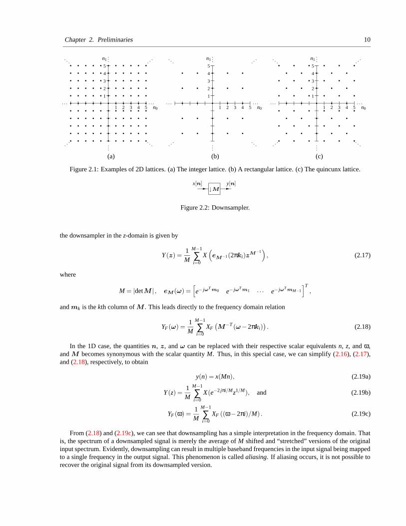
Figure 2.1: Examples of 2D lattices. (a) The integer lattice. (b) A rectangular lattice. (c) The quincunx lattice.
↓M- -x[n] y[n]
Figure 2.2: Downsampler.
the downsampler in the z-domain is given by
Y (z) =1M
M−1
∑i=0
X(
eM−1(2πki)z
M−1)
, (2.17)
where
M = |detM | , eM (ω) =[
e− jωTm0 e− jωT
m1 · · · e− jωTmM−1
]T,
and mk is the kth column of M . This leads directly to the frequency domain relation
YF(ω) =1M
M−1
∑i=0
XF(M−T (ω−2πki)
). (2.18)
In the 1D case, the quantities n, z, and ω can be replaced with their respective scalar equivalents n, z, and ω,and M becomes synonymous with the scalar quantity M. Thus, in this special case, we can simplify (2.16), (2.17),and (2.18), respectively, to obtain
y(n) = x(Mn), (2.19a)
Y (z) =1M
M−1
∑i=0
X(e−2 jπi/Mz1/M), and (2.19b)
YF(ω) =1M
M−1
∑i=0
XF ((ω−2πi)/M) . (2.19c)
From (2.18) and (2.19c), we can see that downsampling has a simple interpretation in the frequency domain. Thatis, the spectrum of a downsampled signal is merely the average of M shifted and “stretched” versions of the originalinput spectrum. Evidently, downsampling can result in multiple baseband frequencies in the input signal being mappedto a single frequency in the output signal. This phenomenon is called aliasing. If aliasing occurs, it is not possible torecover the original signal from its downsampled version.
Chapter 2. Preliminaries 11
↑M- -x[n] y[n]
Figure 2.3: Upsampler.
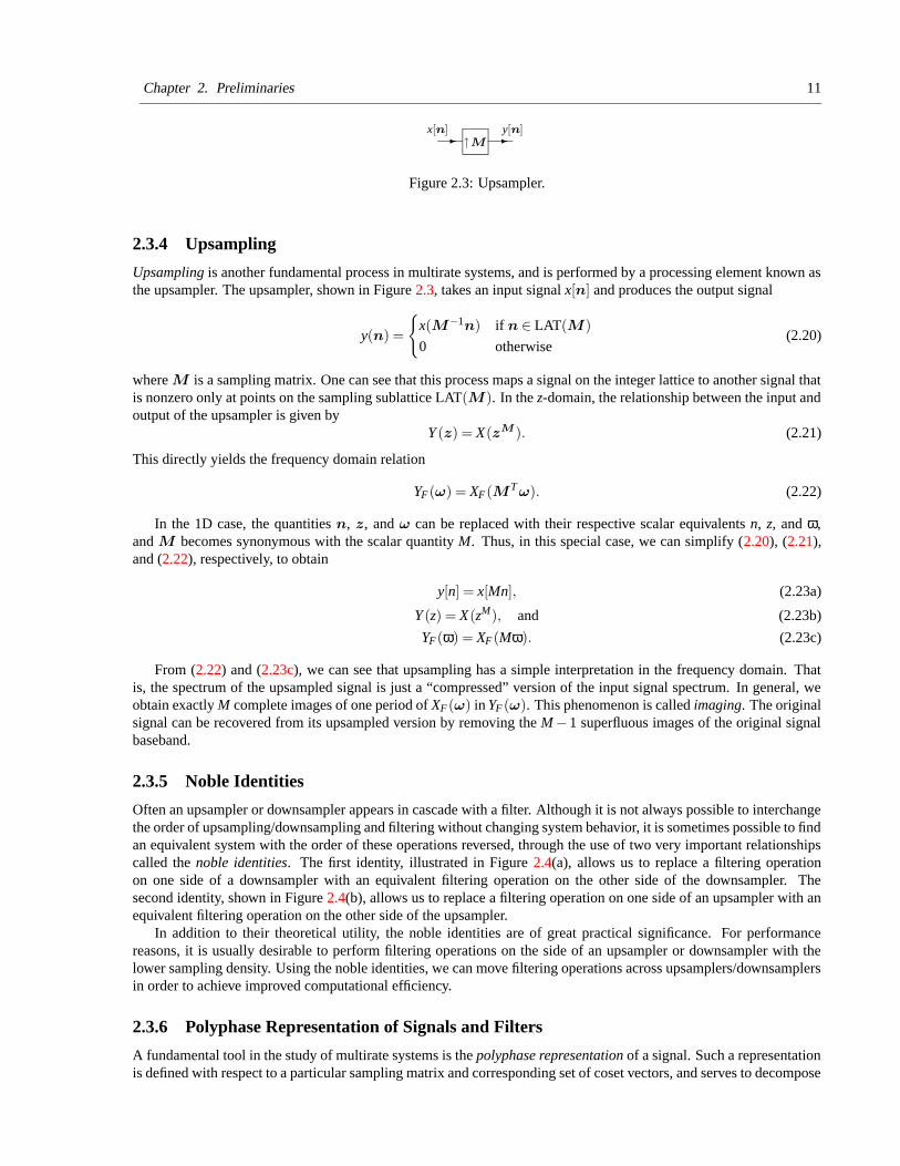
2.3.4 Upsampling
Upsampling is another fundamental process in multirate systems, and is performed by a processing element known asthe upsampler. The upsampler, shown in Figure 2.3, takes an input signal x[n] and produces the output signal
y(n) =
{
x(M−1n) if n ∈ LAT(M)
0 otherwise(2.20)
where M is a sampling matrix. One can see that this process maps a signal on the integer lattice to another signal thatis nonzero only at points on the sampling sublattice LAT(M). In the z-domain, the relationship between the input andoutput of the upsampler is given by
Y (z) = X(zM ). (2.21)
This directly yields the frequency domain relation
YF(ω) = XF(MT ω). (2.22)
In the 1D case, the quantities n, z, and ω can be replaced with their respective scalar equivalents n, z, and ω,and M becomes synonymous with the scalar quantity M. Thus, in this special case, we can simplify (2.20), (2.21),and (2.22), respectively, to obtain
y[n] = x[Mn], (2.23a)
Y (z) = X(zM), and (2.23b)
YF(ω) = XF(Mω). (2.23c)
From (2.22) and (2.23c), we can see that upsampling has a simple interpretation in the frequency domain. Thatis, the spectrum of the upsampled signal is just a “compressed” version of the input signal spectrum. In general, weobtain exactly M complete images of one period of XF(ω) in YF(ω). This phenomenon is called imaging. The originalsignal can be recovered from its upsampled version by removing the M −1 superfluous images of the original signalbaseband.
2.3.5 Noble Identities
Often an upsampler or downsampler appears in cascade with a filter. Although it is not always possible to interchangethe order of upsampling/downsampling and filtering without changing system behavior, it is sometimes possible to findan equivalent system with the order of these operations reversed, through the use of two very important relationshipscalled the noble identities. The first identity, illustrated in Figure 2.4(a), allows us to replace a filtering operationon one side of a downsampler with an equivalent filtering operation on the other side of the downsampler. Thesecond identity, shown in Figure 2.4(b), allows us to replace a filtering operation on one side of an upsampler with anequivalent filtering operation on the other side of the upsampler.
In addition to their theoretical utility, the noble identities are of great practical significance. For performancereasons, it is usually desirable to perform filtering operations on the side of an upsampler or downsampler with thelower sampling density. Using the noble identities, we can move filtering operations across upsamplers/downsamplersin order to achieve improved computational efficiency.
2.3.6 Polyphase Representation of Signals and Filters
A fundamental tool in the study of multirate systems is the polyphase representation of a signal. Such a representationis defined with respect to a particular sampling matrix and corresponding set of coset vectors, and serves to decompose
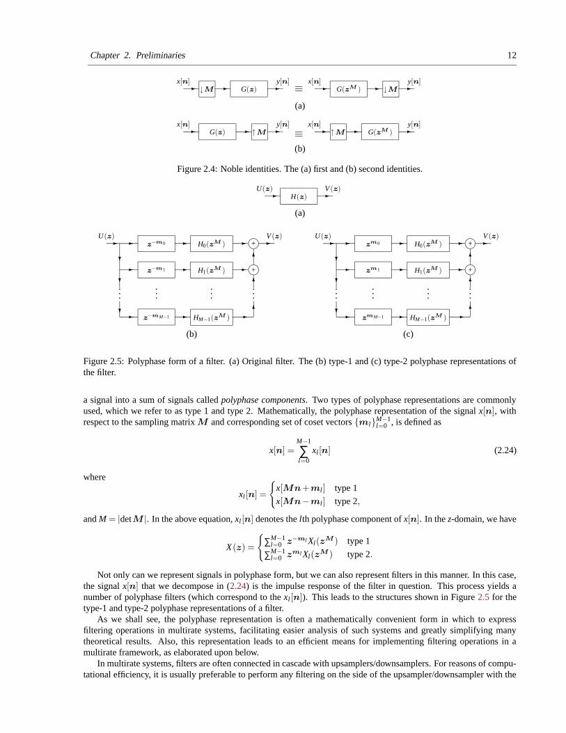
Chapter 2. Preliminaries 12
-- - - - -G(z) ≡x[n] y[n]G(zM )
x[n] y[n]↓M ↓M
(a)
- - - - --G(z) ≡ G(zM )x[n] y[n] x[n] y[n]
↑M ↑M
(b)
Figure 2.4: Noble identities. The (a) first and (b) second identities.
- -H(z)V (z)U(z)
(a)
j+
j+-
-
-
-
-
-?
?
?
-
-
-
- -
6
6
6
......
U(z)z−m0
z−mM−1
z−m1
HM−1(zM )
...
H1(zM )
H0(zM )
...
V (z)
(b)
j+
j+-
-
-
-
-
-?
?
?
-
-
-
- -
6
6
6
......
U(z)z
m0
zmM−1
zm1
HM−1(zM )
...
H1(zM )
H0(zM )
...
V (z)
(c)
Figure 2.5: Polyphase form of a filter. (a) Original filter. The (b) type-1 and (c) type-2 polyphase representations ofthe filter.
a signal into a sum of signals called polyphase components. Two types of polyphase representations are commonlyused, which we refer to as type 1 and type 2. Mathematically, the polyphase representation of the signal x[n], withrespect to the sampling matrix M and corresponding set of coset vectors {ml}M−1
l=0 , is defined as
x[n] =M−1
∑l=0
xl [n] (2.24)
where
xl [n] =
{
x[Mn+ml ] type 1
x[Mn−ml ] type 2,
and M = |detM |. In the above equation, xl [n] denotes the lth polyphase component of x[n]. In the z-domain, we have
X(z) =
{
∑M−1l=0 z−ml Xl(z
M ) type 1
∑M−1l=0 zml Xl(z
M ) type 2.
Not only can we represent signals in polyphase form, but we can also represent filters in this manner. In this case,the signal x[n] that we decompose in (2.24) is the impulse response of the filter in question. This process yields anumber of polyphase filters (which correspond to the xl [n]). This leads to the structures shown in Figure 2.5 for thetype-1 and type-2 polyphase representations of a filter.
As we shall see, the polyphase representation is often a mathematically convenient form in which to expressfiltering operations in multirate systems, facilitating easier analysis of such systems and greatly simplifying manytheoretical results. Also, this representation leads to an efficient means for implementing filtering operations in amultirate framework, as elaborated upon below.
In multirate systems, filters are often connected in cascade with upsamplers/downsamplers. For reasons of compu-tational efficiency, it is usually preferable to perform any filtering on the side of the upsampler/downsampler with the
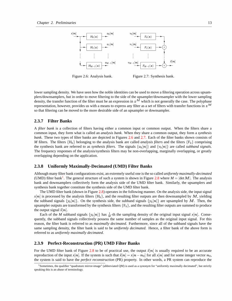
Chapter 2. Preliminaries 13
?
?
- -
-
-
?
-
-
-
H0(z)
H1(z)
HM−1(z)
......
...
x[n] u0[n]
u1[n]
uM−1[n]
Figure 2.6: Analysis bank.
j+
j+-
-
-
-
-
-
-
?
?
?F0(z)
F1(z)
...
FM−1(z)
......
v0[n]
v1[n]
vM−1[n] x[n]
Figure 2.7: Synthesis bank.
lower sampling density. We have seen how the noble identities can be used to move a filtering operation across upsam-plers/downsamplers, but in order to move filtering to the side of the upsampler/downsampler with the lower samplingdensity, the transfer function of the filter must be an expression in zM which is not generally the case. The polyphaserepresentation, however, provides us with a means to express any filter as a set of filters with transfer functions in zM
so that filtering can be moved to the more desirable side of an upsampler or downsampler.
2.3.7 Filter Banks
A filter bank is a collection of filters having either a common input or common output. When the filters share acommon input, they form what is called an analysis bank. When they share a common output, they form a synthesisbank. These two types of filter banks are depicted in Figures 2.6 and 2.7. Each of the filter banks shown consists ofM filters. The filters {Hk} belonging to the analysis bank are called analysis filters and the filters {Fk} comprisingthe synthesis bank are referred to as synthesis filters. The signals {uk[n]} and {vk[n]} are called subband signals.The frequency responses of the analysis/synthesis filters may be non-overlapping, marginally overlapping, or greatlyoverlapping depending on the application.
2.3.8 Uniformly Maximally-Decimated (UMD) Filter Banks
Although many filter bank configurations exist, an extremely useful one is the so called uniformly maximally-decimated(UMD) filter bank1. The general structure of such a system is shown in Figure 2.8 where M = |detM |. The analysisbank and downsamplers collectively form the analysis side of the UMD filter bank. Similarly, the upsamplers andsynthesis bank together constitute the synthesis side of the UMD filter bank.
The UMD filter bank (shown in Figure 2.8) operates in the following manner. On the analysis side, the input signalx[n] is processed by the analysis filters {Hk}, and the resulting filter outputs are then downsampled by M , yieldingthe subband signals {yk[n]}. On the synthesis side, the subband signals {yk[n]} are upsampled by M . Then, theupsampler outputs are transformed by the synthesis filters {Fk}, and the resulting filter outputs are summed to producethe output signal x[n].
Each of the M subband signals {yk[n]} has 1M -th the sampling density of the original input signal x[n]. Conse-
quently, the subband signals collectively possess the same number of samples as the original input signal. For thisreason, the filter bank is referred to as maximally decimated. Furthermore, since all of the subband signals have thesame sampling density, the filter bank is said to be uniformly decimated. Hence, a filter bank of the above form isreferred to as uniformly maximally decimated.
2.3.9 Perfect-Reconstruction (PR) UMD Filter Banks
For the UMD filter bank of Figure 2.8 to be of practical use, the output x[n] is usually required to be an accuratereproduction of the input x[n]. If the system is such that x[n] = x[n−n0] for all x[n] and for some integer vector n0,the system is said to have the perfect reconstruction (PR) property. In other words, a PR system can reproduce the
1Sometimes, the qualifier “quadrature mirror-image” (abbreviated QM) is used as a synonym for “uniformly maximally decimated”, but strictlyspeaking this is an abuse of terminology.
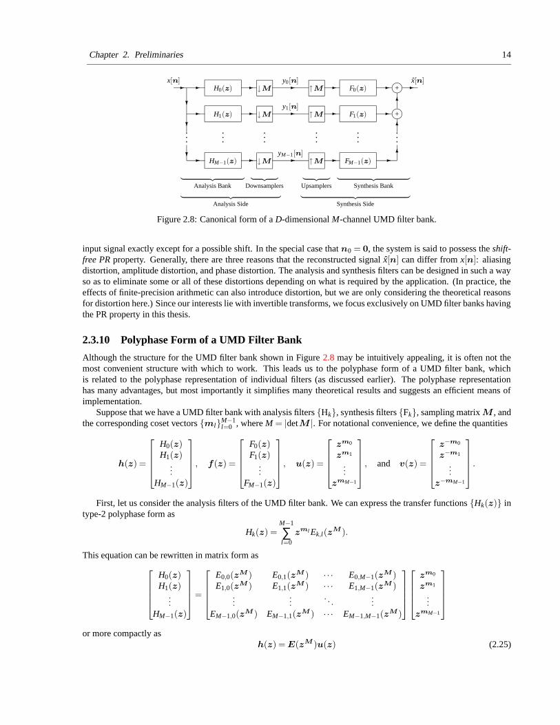
Chapter 2. Preliminaries 14
j+
j+-
-
-
-
-
-
-
-
-
-
-
-
-?
?
?
-
-
- -
6
6
6
H0(z) F0(z)
F1(z)H1(z)
...
HM−1(z)
......
FM−1(z)
......
...
x[n]↓M
↓M
↓M ↑M
↑M
↑M
x[n]
︸ ︷︷ ︸
Analysis Bank︸ ︷︷ ︸
Downsamplers︸ ︷︷ ︸
Upsamplers︸ ︷︷ ︸
Synthesis Bank
y0[n]
y1[n]
yM−1[n]
︸ ︷︷ ︸
Analysis Side︸ ︷︷ ︸
Synthesis Side
Figure 2.8: Canonical form of a D-dimensional M-channel UMD filter bank.
input signal exactly except for a possible shift. In the special case that n0 = 0, the system is said to possess the shift-free PR property. Generally, there are three reasons that the reconstructed signal x[n] can differ from x[n]: aliasingdistortion, amplitude distortion, and phase distortion. The analysis and synthesis filters can be designed in such a wayso as to eliminate some or all of these distortions depending on what is required by the application. (In practice, theeffects of finite-precision arithmetic can also introduce distortion, but we are only considering the theoretical reasonsfor distortion here.) Since our interests lie with invertible transforms, we focus exclusively on UMD filter banks havingthe PR property in this thesis.
2.3.10 Polyphase Form of a UMD Filter Bank
Although the structure for the UMD filter bank shown in Figure 2.8 may be intuitively appealing, it is often not themost convenient structure with which to work. This leads us to the polyphase form of a UMD filter bank, whichis related to the polyphase representation of individual filters (as discussed earlier). The polyphase representationhas many advantages, but most importantly it simplifies many theoretical results and suggests an efficient means ofimplementation.
Suppose that we have a UMD filter bank with analysis filters {Hk}, synthesis filters {Fk}, sampling matrix M , andthe corresponding coset vectors {ml}M−1
l=0 , where M = |detM |. For notational convenience, we define the quantities
h(z) =
H0(z)H1(z)
...HM−1(z)
, f(z) =
F0(z)F1(z)
...FM−1(z)
, u(z) =
zm0
zm1
...zmM−1
, and v(z) =
z−m0
z−m1
...z−mM−1
.
First, let us consider the analysis filters of the UMD filter bank. We can express the transfer functions {Hk(z)} intype-2 polyphase form as
Hk(z) =M−1
∑l=0
zml Ek,l(zM ).
This equation can be rewritten in matrix form as
H0(z)H1(z)
...HM−1(z)
=
E0,0(zM ) E0,1(z
M ) · · · E0,M−1(zM )
E1,0(zM ) E1,1(z
M ) · · · E1,M−1(zM )
......
. . ....
EM−1,0(zM ) EM−1,1(z
M ) · · · EM−1,M−1(zM )
zm0
zm1
...zmM−1
or more compactly ash(z) = E(zM )u(z) (2.25)
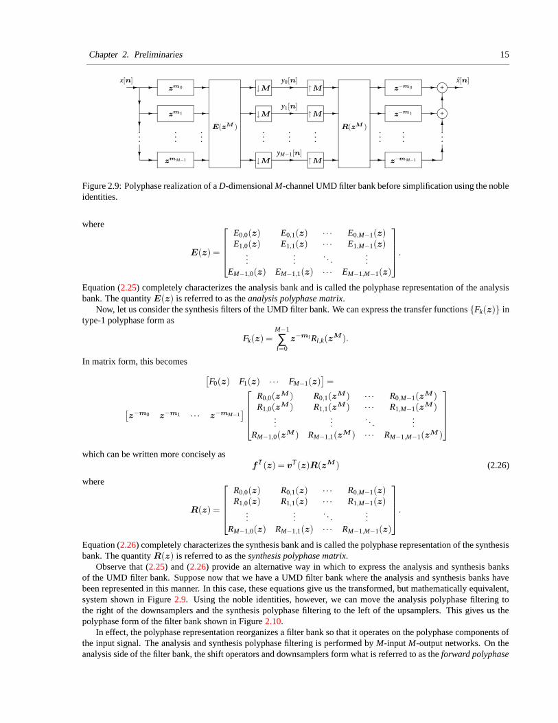
Chapter 2. Preliminaries 15
j+
j+
E(zM )
↓M
↓M
↓M
R(zM )
↑M
↑M
↑M
-
-
-
-
-
-?
?
?
-
-
-
-
- -
- -
6
6
6
-
-
--
-
- -
-
-
......
x[n]z
m0
zmM−1
zm1
......
x[n]
z−mM−1
z−m1
z−m0
y0[n]
y1[n]
yM−1[n]
......
......
...
Figure 2.9: Polyphase realization of a D-dimensional M-channel UMD filter bank before simplification using the nobleidentities.
where
E(z) =
E0,0(z) E0,1(z) · · · E0,M−1(z)E1,0(z) E1,1(z) · · · E1,M−1(z)
......
. . ....
EM−1,0(z) EM−1,1(z) · · · EM−1,M−1(z)
.
Equation (2.25) completely characterizes the analysis bank and is called the polyphase representation of the analysisbank. The quantity E(z) is referred to as the analysis polyphase matrix.
Now, let us consider the synthesis filters of the UMD filter bank. We can express the transfer functions {Fk(z)} intype-1 polyphase form as
Fk(z) =M−1
∑l=0
z−ml Rl,k(zM ).
In matrix form, this becomes[F0(z) F1(z) · · · FM−1(z)
]=
[z−m0 z−m1 · · · z−mM−1
]
R0,0(zM ) R0,1(z
M ) · · · R0,M−1(zM )
R1,0(zM ) R1,1(z
M ) · · · R1,M−1(zM )
......
. . ....
RM−1,0(zM ) RM−1,1(z
M ) · · · RM−1,M−1(zM )
which can be written more concisely asfT (z) = vT (z)R(zM ) (2.26)
where
R(z) =
R0,0(z) R0,1(z) · · · R0,M−1(z)R1,0(z) R1,1(z) · · · R1,M−1(z)
......
. . ....
RM−1,0(z) RM−1,1(z) · · · RM−1,M−1(z)
.
Equation (2.26) completely characterizes the synthesis bank and is called the polyphase representation of the synthesisbank. The quantity R(z) is referred to as the synthesis polyphase matrix.
Observe that (2.25) and (2.26) provide an alternative way in which to express the analysis and synthesis banksof the UMD filter bank. Suppose now that we have a UMD filter bank where the analysis and synthesis banks havebeen represented in this manner. In this case, these equations give us the transformed, but mathematically equivalent,system shown in Figure 2.9. Using the noble identities, however, we can move the analysis polyphase filtering tothe right of the downsamplers and the synthesis polyphase filtering to the left of the upsamplers. This gives us thepolyphase form of the filter bank shown in Figure 2.10.
In effect, the polyphase representation reorganizes a filter bank so that it operates on the polyphase components ofthe input signal. The analysis and synthesis polyphase filtering is performed by M-input M-output networks. On theanalysis side of the filter bank, the shift operators and downsamplers form what is referred to as the forward polyphase
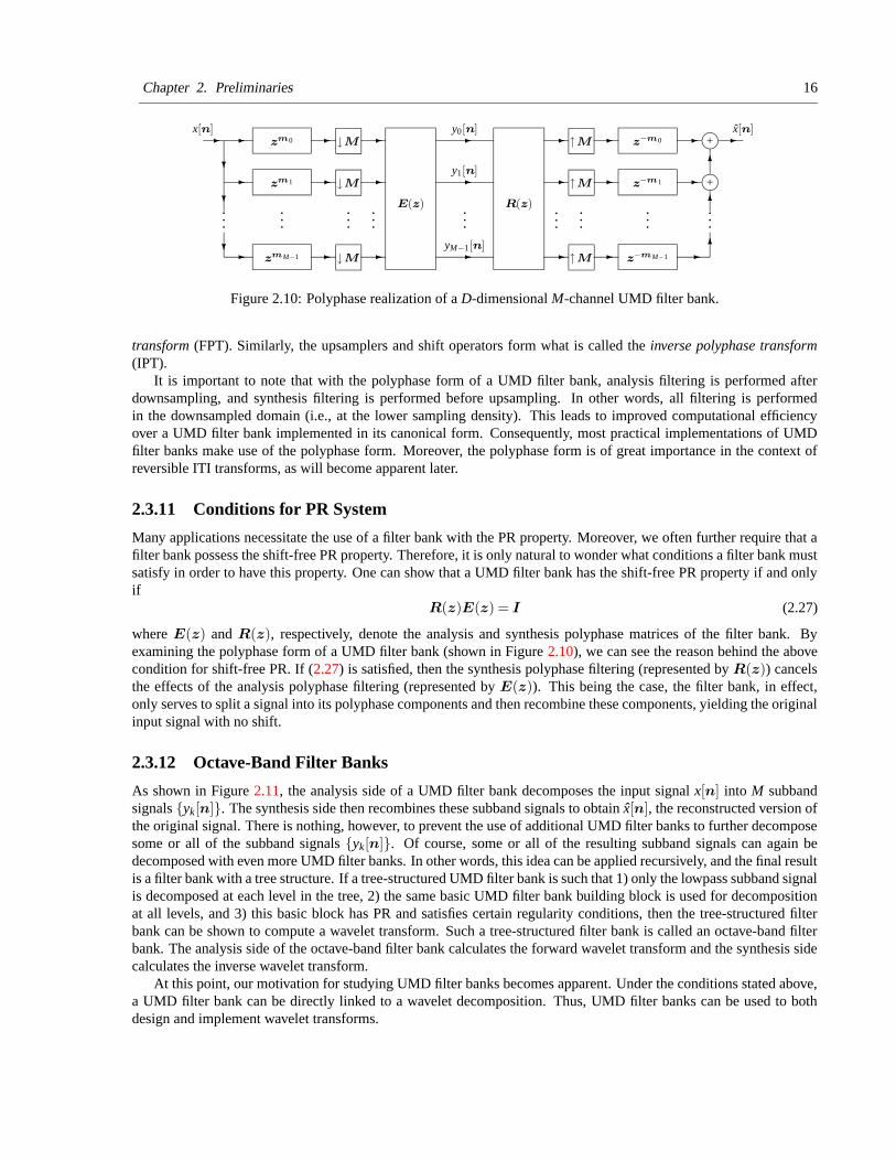
Chapter 2. Preliminaries 16
j+
j+-
-
-
-
-
-?
?
?
-
-
-
-
-
-
-
- -
- -
6
6
6
-
-
--
-
-
E(z)......
...
x[n]↓M
↓M
↓M
zm0
zmM−1
zm1
......
......
↑M
↑M
x[n]
z−mM−1
z−m1
z−m0
↑M
R(z) ...
y0[n]
y1[n]
yM−1[n]
...
Figure 2.10: Polyphase realization of a D-dimensional M-channel UMD filter bank.
transform (FPT). Similarly, the upsamplers and shift operators form what is called the inverse polyphase transform(IPT).
It is important to note that with the polyphase form of a UMD filter bank, analysis filtering is performed afterdownsampling, and synthesis filtering is performed before upsampling. In other words, all filtering is performedin the downsampled domain (i.e., at the lower sampling density). This leads to improved computational efficiencyover a UMD filter bank implemented in its canonical form. Consequently, most practical implementations of UMDfilter banks make use of the polyphase form. Moreover, the polyphase form is of great importance in the context ofreversible ITI transforms, as will become apparent later.
2.3.11 Conditions for PR System
Many applications necessitate the use of a filter bank with the PR property. Moreover, we often further require that afilter bank possess the shift-free PR property. Therefore, it is only natural to wonder what conditions a filter bank mustsatisfy in order to have this property. One can show that a UMD filter bank has the shift-free PR property if and onlyif
R(z)E(z) = I (2.27)
where E(z) and R(z), respectively, denote the analysis and synthesis polyphase matrices of the filter bank. Byexamining the polyphase form of a UMD filter bank (shown in Figure 2.10), we can see the reason behind the abovecondition for shift-free PR. If (2.27) is satisfied, then the synthesis polyphase filtering (represented by R(z)) cancelsthe effects of the analysis polyphase filtering (represented by E(z)). This being the case, the filter bank, in effect,only serves to split a signal into its polyphase components and then recombine these components, yielding the originalinput signal with no shift.
2.3.12 Octave-Band Filter Banks
As shown in Figure 2.11, the analysis side of a UMD filter bank decomposes the input signal x[n] into M subbandsignals {yk[n]}. The synthesis side then recombines these subband signals to obtain x[n], the reconstructed version ofthe original signal. There is nothing, however, to prevent the use of additional UMD filter banks to further decomposesome or all of the subband signals {yk[n]}. Of course, some or all of the resulting subband signals can again bedecomposed with even more UMD filter banks. In other words, this idea can be applied recursively, and the final resultis a filter bank with a tree structure. If a tree-structured UMD filter bank is such that 1) only the lowpass subband signalis decomposed at each level in the tree, 2) the same basic UMD filter bank building block is used for decompositionat all levels, and 3) this basic block has PR and satisfies certain regularity conditions, then the tree-structured filterbank can be shown to compute a wavelet transform. Such a tree-structured filter bank is called an octave-band filterbank. The analysis side of the octave-band filter bank calculates the forward wavelet transform and the synthesis sidecalculates the inverse wavelet transform.
At this point, our motivation for studying UMD filter banks becomes apparent. Under the conditions stated above,a UMD filter bank can be directly linked to a wavelet decomposition. Thus, UMD filter banks can be used to bothdesign and implement wavelet transforms.
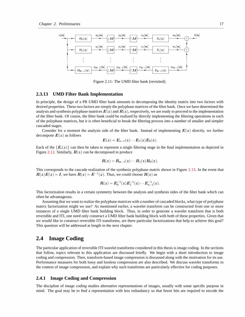
Chapter 2. Preliminaries 17
j+
j+-
-
-?
?
?
- - --
-
-
-
-
-
-
-
-
-
-
6
6
6
H0(z)
H1(z)
...
HM−1(z)
......
......
...
FM−1(z)
F1(z)
uM−1[n]
F0(z)
u1[n]
u0[n] y0[n]
y1[n]
yM−1[n]
v0[n]
v1[n]
vM−1[n]
w0[n]
w1[n]
wM−1[n]
x[n]
↓M
↓M
↓M ↑M
↑M
↑M
x[n]
Figure 2.11: The UMD filter bank (revisited).
2.3.13 UMD Filter Bank Implementation
In principle, the design of a PR UMD filter bank amounts to decomposing the identity matrix into two factors withdesired properties. These two factors are simply the polyphase matrices of the filter bank. Once we have determined theanalysis and synthesis polyphase matrices E(z) and R(z), respectively, we are ready to proceed to the implementationof the filter bank. Of course, the filter bank could be realized by directly implementing the filtering operations in eachof the polyphase matrices, but it is often beneficial to break the filtering process into a number of smaller and simplercascaded stages.
Consider for a moment the analysis side of the filter bank. Instead of implementing E(z) directly, we furtherdecompose E(z) as follows
E(z) = En−1(z) · · ·E1(z)E0(z).
Each of the {Ei(z)} can then be taken to represent a single filtering stage in the final implementation as depicted inFigure 2.12. Similarly, R(z) can be decomposed to produce
R(z) = Rm−1(z) · · ·R1(z)R0(z).
This corresponds to the cascade realization of the synthesis polyphase matrix shown in Figure 2.13. In the event thatR(z)E(z) = I , we have R(z) = E−1(z). Thus, we could choose R(z) as
R(z) = E−10 (z)E−1
1 (z) · · ·E−1n−1(z).
This factorization results in a certain symmetry between the analysis and synthesis sides of the filter bank which canoften be advantageous.
Assuming that we want to realize the polyphase matrices with a number of cascaded blocks, what type of polyphasematrix factorization might we use? As mentioned earlier, a wavelet transform can be constructed from one or moreinstances of a single UMD filter bank building block. Thus, in order to generate a wavelet transform that is bothreversible and ITI, one need only construct a UMD filter bank building block with both of these properties. Given thatwe would like to construct reversible ITI transforms, are there particular factorizations that help to achieve this goal?This question will be addressed at length in the next chapter.
2.4 Image Coding
The particular application of reversible ITI wavelet transforms considered in this thesis is image coding. In the sectionsthat follow, topics relevant to this application are discussed briefly. We begin with a short introduction to imagecoding and compression. Then, transform-based image compression is discussed along with the motivation for its use.Performance measures for both lossy and lossless compression are also described. We discuss wavelet transforms inthe context of image compression, and explain why such transforms are particularly effective for coding purposes.
2.4.1 Image Coding and Compression
The discipline of image coding studies alternative representations of images, usually with some specific purpose inmind. The goal may be to find a representation with less redundancy so that fewer bits are required to encode the
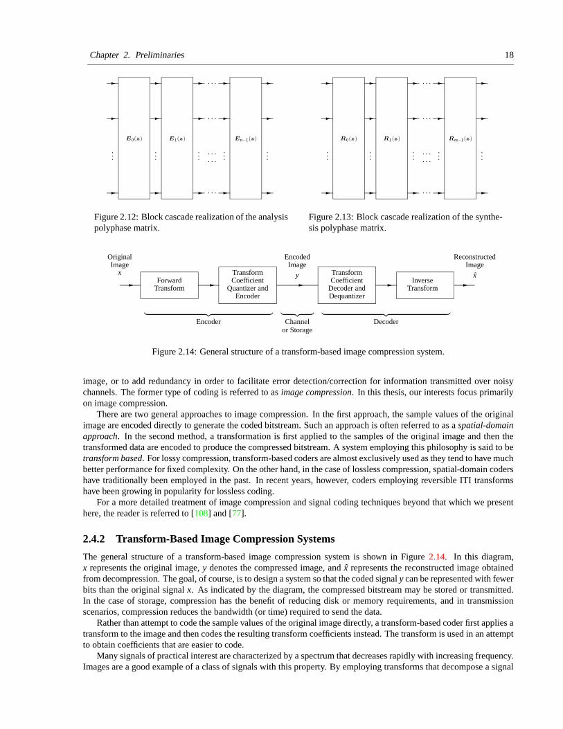
Chapter 2. Preliminaries 18
-- - --
-
-
-
-
-
-
-
-
-
-
...
E0(z) E1(z)
......
· · ·
En−1(z)
...
· · ·
· · ·
...· · ·· · ·
Figure 2.12: Block cascade realization of the analysispolyphase matrix.
-- - --
-
-
-
-
-
-
-
-
-
-
......
...
· · ·
...
· · ·
· · ·
...· · ·· · ·
R0(z) R1(z) Rm−1(z)
Figure 2.13: Block cascade realization of the synthe-sis polyphase matrix.
-- -- -TransformForward Inverse
Transform
yTransformCoefficient
Quantizer andEncoder
TransformCoefficient
Decoder andDequantizer
or Storage
︸ ︷︷ ︸
Encoder︸ ︷︷ ︸
Channel︸ ︷︷ ︸
Decoder
Original Encoded Reconstructed
xxImage Image Image
Figure 2.14: General structure of a transform-based image compression system.
image, or to add redundancy in order to facilitate error detection/correction for information transmitted over noisychannels. The former type of coding is referred to as image compression. In this thesis, our interests focus primarilyon image compression.
There are two general approaches to image compression. In the first approach, the sample values of the originalimage are encoded directly to generate the coded bitstream. Such an approach is often referred to as a spatial-domainapproach. In the second method, a transformation is first applied to the samples of the original image and then thetransformed data are encoded to produce the compressed bitstream. A system employing this philosophy is said to betransform based. For lossy compression, transform-based coders are almost exclusively used as they tend to have muchbetter performance for fixed complexity. On the other hand, in the case of lossless compression, spatial-domain codershave traditionally been employed in the past. In recent years, however, coders employing reversible ITI transformshave been growing in popularity for lossless coding.
For a more detailed treatment of image compression and signal coding techniques beyond that which we presenthere, the reader is referred to [108] and [77].
2.4.2 Transform-Based Image Compression Systems
The general structure of a transform-based image compression system is shown in Figure 2.14. In this diagram,x represents the original image, y denotes the compressed image, and x represents the reconstructed image obtainedfrom decompression. The goal, of course, is to design a system so that the coded signal y can be represented with fewerbits than the original signal x. As indicated by the diagram, the compressed bitstream may be stored or transmitted.In the case of storage, compression has the benefit of reducing disk or memory requirements, and in transmissionscenarios, compression reduces the bandwidth (or time) required to send the data.
Rather than attempt to code the sample values of the original image directly, a transform-based coder first applies atransform to the image and then codes the resulting transform coefficients instead. The transform is used in an attemptto obtain coefficients that are easier to code.
Many signals of practical interest are characterized by a spectrum that decreases rapidly with increasing frequency.Images are a good example of a class of signals with this property. By employing transforms that decompose a signal
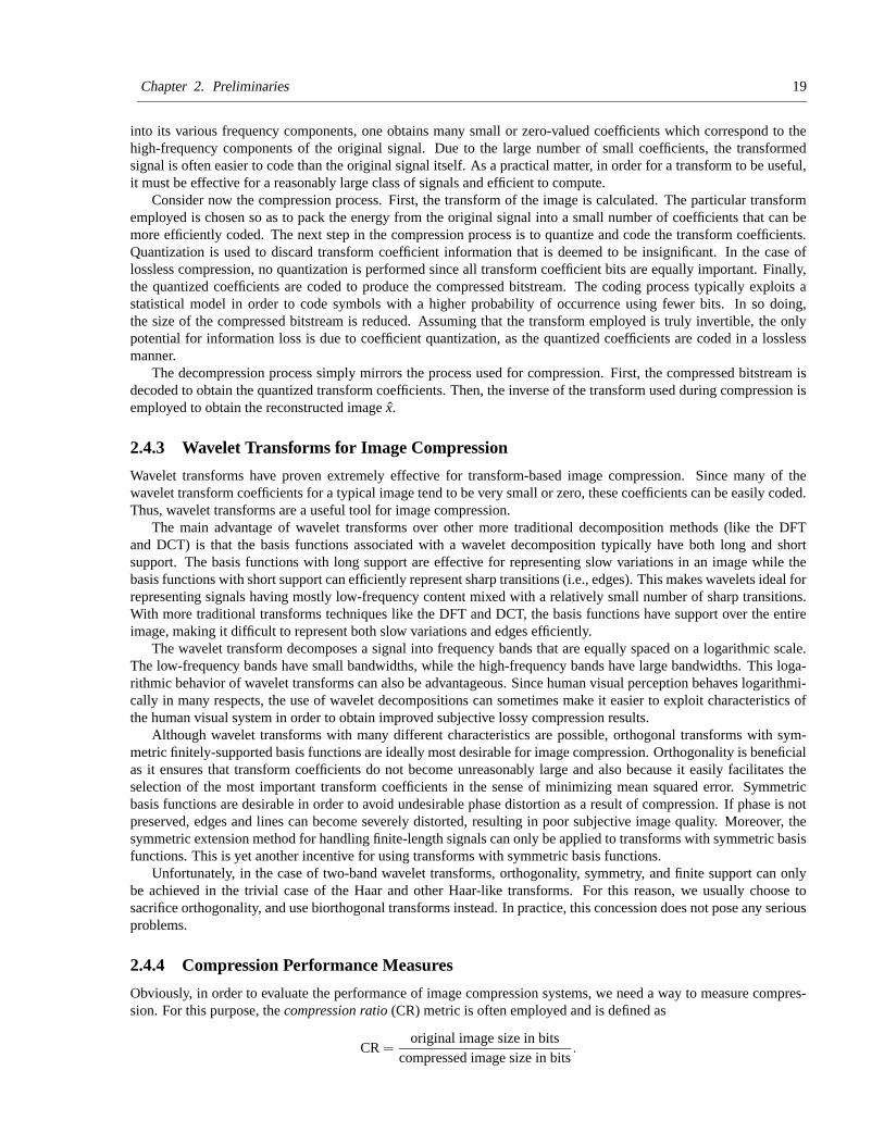
Chapter 2. Preliminaries 19
into its various frequency components, one obtains many small or zero-valued coefficients which correspond to thehigh-frequency components of the original signal. Due to the large number of small coefficients, the transformedsignal is often easier to code than the original signal itself. As a practical matter, in order for a transform to be useful,it must be effective for a reasonably large class of signals and efficient to compute.
Consider now the compression process. First, the transform of the image is calculated. The particular transformemployed is chosen so as to pack the energy from the original signal into a small number of coefficients that can bemore efficiently coded. The next step in the compression process is to quantize and code the transform coefficients.Quantization is used to discard transform coefficient information that is deemed to be insignificant. In the case oflossless compression, no quantization is performed since all transform coefficient bits are equally important. Finally,the quantized coefficients are coded to produce the compressed bitstream. The coding process typically exploits astatistical model in order to code symbols with a higher probability of occurrence using fewer bits. In so doing,the size of the compressed bitstream is reduced. Assuming that the transform employed is truly invertible, the onlypotential for information loss is due to coefficient quantization, as the quantized coefficients are coded in a losslessmanner.
The decompression process simply mirrors the process used for compression. First, the compressed bitstream isdecoded to obtain the quantized transform coefficients. Then, the inverse of the transform used during compression isemployed to obtain the reconstructed image x.
2.4.3 Wavelet Transforms for Image Compression
Wavelet transforms have proven extremely effective for transform-based image compression. Since many of thewavelet transform coefficients for a typical image tend to be very small or zero, these coefficients can be easily coded.Thus, wavelet transforms are a useful tool for image compression.
The main advantage of wavelet transforms over other more traditional decomposition methods (like the DFTand DCT) is that the basis functions associated with a wavelet decomposition typically have both long and shortsupport. The basis functions with long support are effective for representing slow variations in an image while thebasis functions with short support can efficiently represent sharp transitions (i.e., edges). This makes wavelets ideal forrepresenting signals having mostly low-frequency content mixed with a relatively small number of sharp transitions.With more traditional transforms techniques like the DFT and DCT, the basis functions have support over the entireimage, making it difficult to represent both slow variations and edges efficiently.
The wavelet transform decomposes a signal into frequency bands that are equally spaced on a logarithmic scale.The low-frequency bands have small bandwidths, while the high-frequency bands have large bandwidths. This loga-rithmic behavior of wavelet transforms can also be advantageous. Since human visual perception behaves logarithmi-cally in many respects, the use of wavelet decompositions can sometimes make it easier to exploit characteristics ofthe human visual system in order to obtain improved subjective lossy compression results.
Although wavelet transforms with many different characteristics are possible, orthogonal transforms with sym-metric finitely-supported basis functions are ideally most desirable for image compression. Orthogonality is beneficialas it ensures that transform coefficients do not become unreasonably large and also because it easily facilitates theselection of the most important transform coefficients in the sense of minimizing mean squared error. Symmetricbasis functions are desirable in order to avoid undesirable phase distortion as a result of compression. If phase is notpreserved, edges and lines can become severely distorted, resulting in poor subjective image quality. Moreover, thesymmetric extension method for handling finite-length signals can only be applied to transforms with symmetric basisfunctions. This is yet another incentive for using transforms with symmetric basis functions.
Unfortunately, in the case of two-band wavelet transforms, orthogonality, symmetry, and finite support can onlybe achieved in the trivial case of the Haar and other Haar-like transforms. For this reason, we usually choose tosacrifice orthogonality, and use biorthogonal transforms instead. In practice, this concession does not pose any seriousproblems.
2.4.4 Compression Performance Measures
Obviously, in order to evaluate the performance of image compression systems, we need a way to measure compres-sion. For this purpose, the compression ratio (CR) metric is often employed and is defined as
CR =original image size in bits
compressed image size in bits.
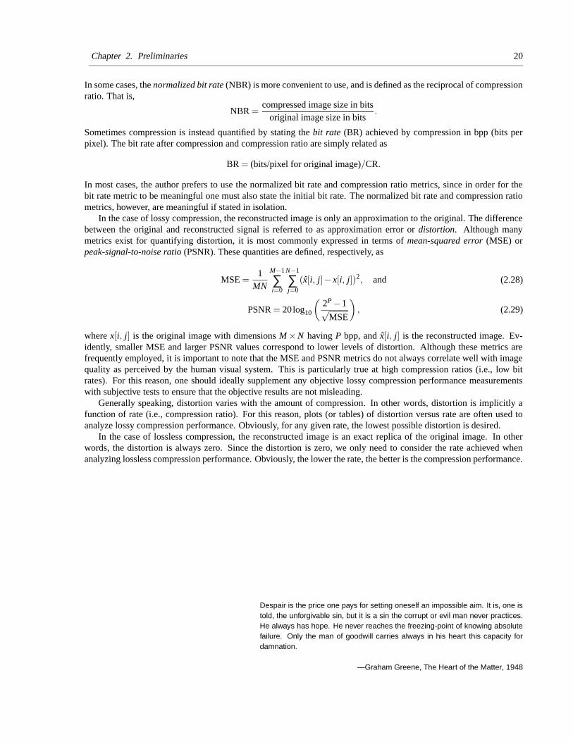
Chapter 2. Preliminaries 20
In some cases, the normalized bit rate (NBR) is more convenient to use, and is defined as the reciprocal of compressionratio. That is,
NBR =compressed image size in bits
original image size in bits.
Sometimes compression is instead quantified by stating the bit rate (BR) achieved by compression in bpp (bits perpixel). The bit rate after compression and compression ratio are simply related as
BR = (bits/pixel for original image)/CR.
In most cases, the author prefers to use the normalized bit rate and compression ratio metrics, since in order for thebit rate metric to be meaningful one must also state the initial bit rate. The normalized bit rate and compression ratiometrics, however, are meaningful if stated in isolation.
In the case of lossy compression, the reconstructed image is only an approximation to the original. The differencebetween the original and reconstructed signal is referred to as approximation error or distortion. Although manymetrics exist for quantifying distortion, it is most commonly expressed in terms of mean-squared error (MSE) orpeak-signal-to-noise ratio (PSNR). These quantities are defined, respectively, as
MSE =1
MN
M−1
∑i=0
N−1
∑j=0
(x[i, j]− x[i, j])2, and (2.28)
PSNR = 20log10
(2P −1√
MSE
)
, (2.29)
where x[i, j] is the original image with dimensions M ×N having P bpp, and x[i, j] is the reconstructed image. Ev-idently, smaller MSE and larger PSNR values correspond to lower levels of distortion. Although these metrics arefrequently employed, it is important to note that the MSE and PSNR metrics do not always correlate well with imagequality as perceived by the human visual system. This is particularly true at high compression ratios (i.e., low bitrates). For this reason, one should ideally supplement any objective lossy compression performance measurementswith subjective tests to ensure that the objective results are not misleading.
Generally speaking, distortion varies with the amount of compression. In other words, distortion is implicitly afunction of rate (i.e., compression ratio). For this reason, plots (or tables) of distortion versus rate are often used toanalyze lossy compression performance. Obviously, for any given rate, the lowest possible distortion is desired.
In the case of lossless compression, the reconstructed image is an exact replica of the original image. In otherwords, the distortion is always zero. Since the distortion is zero, we only need to consider the rate achieved whenanalyzing lossless compression performance. Obviously, the lower the rate, the better is the compression performance.
Despair is the price one pays for setting oneself an impossible aim. It is, one istold, the unforgivable sin, but it is a sin the corrupt or evil man never practices.He always has hope. He never reaches the freezing-point of knowing absolutefailure. Only the man of goodwill carries always in his heart this capacity fordamnation.
—Graham Greene, The Heart of the Matter, 1948
21
Chapter 3
Frameworks for Reversible ITIWavelet/Block Transforms
Wednesday night I fell asleep naturally, exhausted, but woke up with the most intense feeling ofsadness . . . fragments of dreams spinning into lonely wakefulness . . . Do you know what it’s like tobe sad like that? As if your best friend had just died, except the sorrow is worse because that’s notwhat happened, because even while people are leaving you you’ve always been alone.
—Evelyn Lau, Runaway: Diary of a Street Kid, 1989
Overview
The generalized reversible ITI transform (GRITIT) framework, a single unified framework for reversible ITI wavelet/blocktransforms, is proposed. This new framework is then used to study several previously proposed frameworks and theirinterrelationships. For example, the framework based on the overlapping rounding transform is shown to be a spe-cial case of the lifting framework with only trivial extensions. The applicability of the GRITIT framework for blocktransforms is also demonstrated. The generalized S transform (GST), a family of reversible ITI block transforms, isproposed. This family of transforms is then studied in detail. Throughout all of this work, particularly close attentionis paid to rounding operators and their characteristics.
3.1 Introduction
Although reversible ITI wavelet transforms can be constructed using ad-hoc methods, a more structured approach tothe design of such transforms is clearly advantageous. By using a highly structured approach to transform design, wecan produce more sophisticated transforms than is possible with ad-hoc methods. Thus, general frameworks for theconstruction of reversible ITI wavelet transforms are of great interest.
In this chapter, we consider frameworks for the construction of reversible ITI wavelet transforms. We begin, inSection 3.2, by studying one of the key elements in such frameworks, namely rounding operators. This study ofrounding operators will prove quite useful at various junctures in this thesis. In Section 3.3, we examine several pre-viously proposed frameworks. Then, in Section 3.4, we integrate and extend the key concepts from these frameworksin order to form a single unified framework, known as the generalized reversible ITI transform (GRITIT) framework.The GRITIT framework is then used, in Section 3.5, to study the relationships between the various other frameworksintroduced in Section 3.3. Next, Section 3.7 demonstrates the applicability of the GRITIT framework to the designof reversible ITI block transforms. In this context, we propose and study the generalized S transform (GST), a newfamily of reversible ITI block transforms. Finally, in Section 3.8, we summarize the results of this chapter. In passing,we would like to note that some of our results presented in this chapter have also been published in [10, 17, 15, 18].
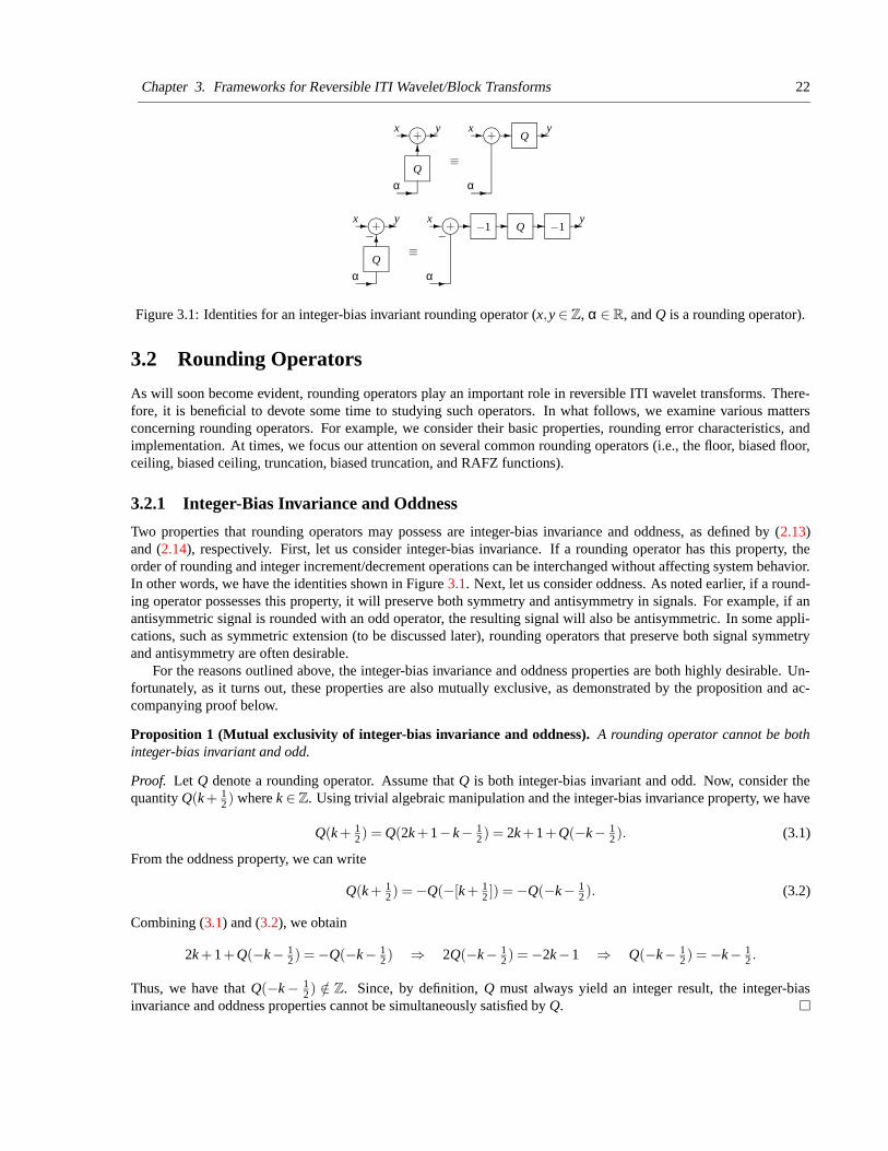
Chapter 3. Frameworks for Reversible ITI Wavelet/Block Transforms 22
j+
Q
j+ Q−1 −1
j+
Q
j+ Q
-
----
-
-- -
6
- -
-
6
- - -
-
≡
α
x y x y
α
−
≡
αα
x y x y
−
Figure 3.1: Identities for an integer-bias invariant rounding operator (x,y ∈ Z, α ∈ R, and Q is a rounding operator).
3.2 Rounding Operators
As will soon become evident, rounding operators play an important role in reversible ITI wavelet transforms. There-fore, it is beneficial to devote some time to studying such operators. In what follows, we examine various mattersconcerning rounding operators. For example, we consider their basic properties, rounding error characteristics, andimplementation. At times, we focus our attention on several common rounding operators (i.e., the floor, biased floor,ceiling, biased ceiling, truncation, biased truncation, and RAFZ functions).
3.2.1 Integer-Bias Invariance and Oddness
Two properties that rounding operators may possess are integer-bias invariance and oddness, as defined by (2.13)and (2.14), respectively. First, let us consider integer-bias invariance. If a rounding operator has this property, theorder of rounding and integer increment/decrement operations can be interchanged without affecting system behavior.In other words, we have the identities shown in Figure 3.1. Next, let us consider oddness. As noted earlier, if a round-ing operator possesses this property, it will preserve both symmetry and antisymmetry in signals. For example, if anantisymmetric signal is rounded with an odd operator, the resulting signal will also be antisymmetric. In some appli-cations, such as symmetric extension (to be discussed later), rounding operators that preserve both signal symmetryand antisymmetry are often desirable.
For the reasons outlined above, the integer-bias invariance and oddness properties are both highly desirable. Un-fortunately, as it turns out, these properties are also mutually exclusive, as demonstrated by the proposition and ac-companying proof below.
Proposition 1 (Mutual exclusivity of integer-bias invariance and oddness). A rounding operator cannot be bothinteger-bias invariant and odd.
Proof. Let Q denote a rounding operator. Assume that Q is both integer-bias invariant and odd. Now, consider thequantity Q(k + 1
2 ) where k ∈ Z. Using trivial algebraic manipulation and the integer-bias invariance property, we have
Q(k + 12 ) = Q(2k +1− k− 1
2 ) = 2k +1+Q(−k− 12 ). (3.1)
From the oddness property, we can write
Q(k + 12 ) = −Q(−[k + 1
2 ]) = −Q(−k− 12 ). (3.2)
Combining (3.1) and (3.2), we obtain
2k +1+Q(−k− 12 ) = −Q(−k− 1
2 ) ⇒ 2Q(−k− 12 ) = −2k−1 ⇒ Q(−k− 1
2 ) = −k− 12 .
Thus, we have that Q(−k − 12 ) /∈ Z. Since, by definition, Q must always yield an integer result, the integer-bias
invariance and oddness properties cannot be simultaneously satisfied by Q.
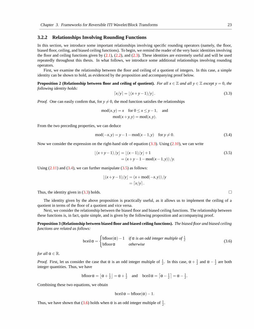
Chapter 3. Frameworks for Reversible ITI Wavelet/Block Transforms 23
3.2.2 Relationships Involving Rounding Functions
In this section, we introduce some important relationships involving specific rounding operators (namely, the floor,biased floor, ceiling, and biased ceiling functions). To begin, we remind the reader of the very basic identities involvingthe floor and ceiling functions given by (2.1), (2.2), and (2.3). These identities are extremely useful and will be usedrepeatedly throughout this thesis. In what follows, we introduce some additional relationships involving roundingoperators.
First, we examine the relationship between the floor and ceiling of a quotient of integers. In this case, a simpleidentity can be shown to hold, as evidenced by the proposition and accompanying proof below.
Proposition 2 (Relationship between floor and ceiling of quotient). For all x ∈ Z and all y ∈ Z except y = 0, thefollowing identity holds:
dx/ye = b(x+ y−1)/yc . (3.3)
Proof. One can easily confirm that, for y 6= 0, the mod function satisfies the relationships
mod(x,y) = x for 0 ≤ x ≤ y−1, and
mod(x+ y,y) = mod(x,y).
From the two preceding properties, we can deduce
mod(−x,y) = y−1−mod(x−1,y) for y 6= 0. (3.4)
Now we consider the expression on the right-hand side of equation (3.3). Using (2.10), we can write
b(x+ y−1)/yc = b(x−1)/yc+1 (3.5)
= (x+ y−1−mod(x−1,y))/y.
Using (2.11) and (3.4), we can further manipulate (3.5) as follows:
b(x+ y−1)/yc = (x+mod(−x,y))/y
= dx/ye .
Thus, the identity given in (3.3) holds.
The identity given by the above proposition is practically useful, as it allows us to implement the ceiling of aquotient in terms of the floor of a quotient and vice versa.
Next, we consider the relationship between the biased floor and biased ceiling functions. The relationship betweenthese functions is, in fact, quite simple, and is given by the following proposition and accompanying proof.
Proposition 3 (Relationship between biased floor and biased ceiling functions). The biased floor and biased ceilingfunctions are related as follows:
bceilα =
{
bfloor(α)−1 if α is an odd integer multiple of 12
bfloorα otherwise(3.6)
for all α ∈ R.
Proof. First, let us consider the case that α is an odd integer multiple of 12 . In this case, α + 1
2 and α− 12 are both
integer quantities. Thus, we have
bfloorα =⌊α+ 1
2
⌋= α+ 1
2 and bceilα =⌈α− 1
2
⌉= α− 1
2 .
Combining these two equations, we obtain
bceilα = bfloor(α)−1.
Thus, we have shown that (3.6) holds when α is an odd integer multiple of 12 .

Chapter 3. Frameworks for Reversible ITI Wavelet/Block Transforms 24
Now, let us consider the case that α is not an odd integer multiple of 12 . In this case, we have
bfloorα =⌊α+ 1
2
⌋= α+ 1
2 +∆0 and (3.7)
bceilα =⌈α− 1
2
⌉= α− 1
2 +∆1, (3.8)
where ∆0 and ∆1 are real and satisfy ∆0 ∈ (−1,0) and ∆1 ∈ (0,1). The intervals for ∆0 and ∆1 follow immediatelyfrom the definition of the floor and ceiling functions and the fact that the rounding error cannot be zero since α + 1
2and α− 1
2 cannot be integer quantities. Using simple interval arithmetic, we can deduce from (3.7) and (3.8) that thequantities bfloorα and bceilα must both be contained on the interval (α− 1
2 ,α + 12 ). Since this interval has a width
of one and is open at both ends, however, it cannot contain more than one integer value. Therefore, bfloorα andbceilα, which are integer quantities, must be equal. Thus, we have shown that (3.6) holds when α is not an odd integermultiple of 1
2 , completing the proof.
The identity given by the above proposition is useful in that it allows us to convert expressions using the biasedfloor function to expressions employing the biased ceiling function and vice versa.
In practice, it is frequently necessary to round a real number of the form x2F where x ∈ Z, F ∈ Z, and F ≥ 1 (i.e.,
a dyadic rational number). That is, we often need to compute an expression of the form Q( x2F ) where Q is a rounding
operator. For this reason, we desire some efficient means of evaluating such an expression for various choices of Q.Many of today’s computing platforms utilize two’s complement integer arithmetic. On such platforms, a very efficientmethod exists for computing the floor of a dyadic rational number. This method involves the arithmetic shift right(ASR) operation, and is given by the proposition and accompanying proof below.
Proposition 4 (Relationship between arithmetic right shift and floor of quotient). Suppose that x is an integerrepresented in two’s complement form with a word size of P bits. Let asr(x,n) denote the quantity resulting from thearithmetic right shift of x by n bits. We assert that
asr(x,n) =⌊
x2n
⌋where 0 ≤ n ≤ P−1. (3.9)
Proof. Let a0,a1, . . . ,aP−1 denote the P bits of the word representing x, where a0 and aP−1 are the least- and most-significant bits, respectively. In two’s complement form, the integer x is represented as
x = −aP−12P−1 +∑P−2i=0 ai2i.
Through the properties of modular arithmetic, one can use the preceding equation to show that
mod(x,2n) = ∑n−1i=0 ai2i for 0 ≤ n ≤ P−1. (3.10)
From the definition of the arithmetic shift right operation, we can write (for 0 ≤ n ≤ P−1)
asr(x,n) = −aP−12P−1 +aP−1(
∑P−2i=P−1−n 2i
)+∑P−2−n
i=0 ai+n2i
= −aP−1(2P−1 −2P−1 +2P−1−n)+∑P−2−ni=0 ai+n2i
= −aP−12P−1−n +∑P−2−ni=0 ai+n2i.
Using simple algebraic manipulation, (2.10), and (3.10), we can further rearrange the preceding equation as follows:
asr(x,n) = −aP−12P−1−n +∑P−2−ni=−n ai+n2i −∑−1
i=−n ai+n2i
= 12n (−aP−12P−1 +∑P−2
i=0 ai2i)− 12n mod(x,2n)
= x−mod(x,2n)2n
=⌊
x2n
⌋.
Thus, the identity given in (3.9) holds. (As an aside, we note that (3.9) also trivially holds for n ≥ P. This case,however, is of relatively little practical interest.)
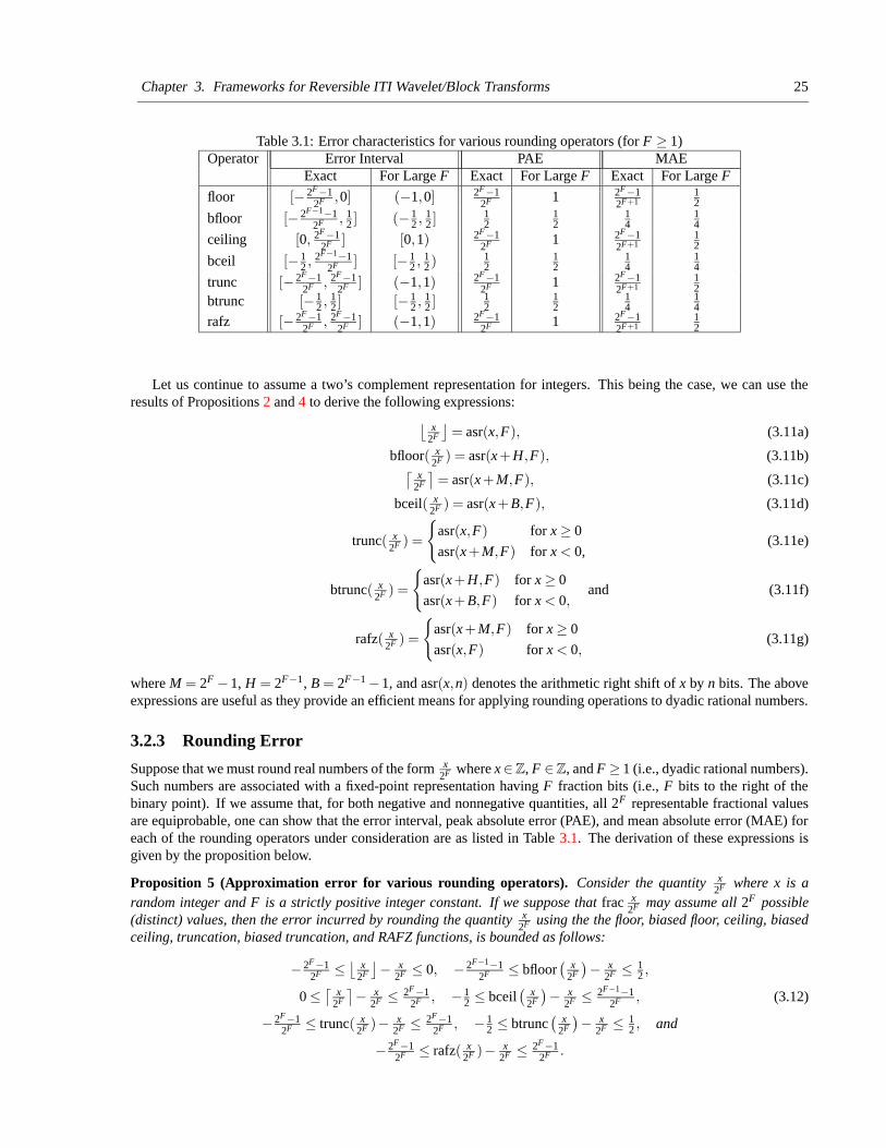
Chapter 3. Frameworks for Reversible ITI Wavelet/Block Transforms 25
Table 3.1: Error characteristics for various rounding operators (for F ≥ 1)Operator Error Interval PAE MAE
Exact For Large F Exact For Large F Exact For Large F
floor [− 2F−12F ,0] (−1,0] 2F−1
2F 1 2F−12F+1
12
bfloor [− 2F−1−12F , 1
2 ] (− 12 , 1
2 ] 12
12
14
14
ceiling [0, 2F−12F ] [0,1) 2F−1
2F 1 2F−12F+1
12
bceil [− 12 , 2F−1−1
2F ] [− 12 , 1
2 ) 12
12
14
14
trunc [− 2F−12F , 2F−1
2F ] (−1,1) 2F−12F 1 2F−1
2F+112
btrunc [− 12 , 1
2 ] [− 12 , 1
2 ] 12
12
14
14
rafz [− 2F−12F , 2F−1
2F ] (−1,1) 2F−12F 1 2F−1
2F+112
Let us continue to assume a two’s complement representation for integers. This being the case, we can use theresults of Propositions 2 and 4 to derive the following expressions:
⌊x
2F
⌋= asr(x,F), (3.11a)
bfloor( x2F ) = asr(x+H,F), (3.11b)
⌈x
2F
⌉= asr(x+M,F), (3.11c)
bceil( x2F ) = asr(x+B,F), (3.11d)
trunc( x2F ) =
{
asr(x,F) for x ≥ 0
asr(x+M,F) for x < 0,(3.11e)
btrunc( x2F ) =
{
asr(x+H,F) for x ≥ 0
asr(x+B,F) for x < 0,and (3.11f)
rafz( x2F ) =
{
asr(x+M,F) for x ≥ 0
asr(x,F) for x < 0,(3.11g)
where M = 2F −1, H = 2F−1, B = 2F−1 −1, and asr(x,n) denotes the arithmetic right shift of x by n bits. The aboveexpressions are useful as they provide an efficient means for applying rounding operations to dyadic rational numbers.
3.2.3 Rounding Error
Suppose that we must round real numbers of the form x2F where x∈Z, F ∈Z, and F ≥ 1 (i.e., dyadic rational numbers).
Such numbers are associated with a fixed-point representation having F fraction bits (i.e., F bits to the right of thebinary point). If we assume that, for both negative and nonnegative quantities, all 2F representable fractional valuesare equiprobable, one can show that the error interval, peak absolute error (PAE), and mean absolute error (MAE) foreach of the rounding operators under consideration are as listed in Table 3.1. The derivation of these expressions isgiven by the proposition below.
Proposition 5 (Approximation error for various rounding operators). Consider the quantity x2F where x is a
random integer and F is a strictly positive integer constant. If we suppose that frac x2F may assume all 2F possible
(distinct) values, then the error incurred by rounding the quantity x2F using the the floor, biased floor, ceiling, biased
ceiling, truncation, biased truncation, and RAFZ functions, is bounded as follows:
− 2F−12F ≤
⌊x
2F
⌋− x
2F ≤ 0, − 2F−1−12F ≤ bfloor
(x
2F
)− x
2F ≤ 12 ,
0 ≤⌈
x2F
⌉− x
2F ≤ 2F−12F , − 1
2 ≤ bceil(
x2F
)− x
2F ≤ 2F−1−12F , (3.12)
− 2F−12F ≤ trunc( x
2F )− x2F ≤ 2F−1
2F , − 12 ≤ btrunc
(x
2F
)− x
2F ≤ 12 , and
− 2F−12F ≤ rafz( x
2F )− x2F ≤ 2F−1
2F .
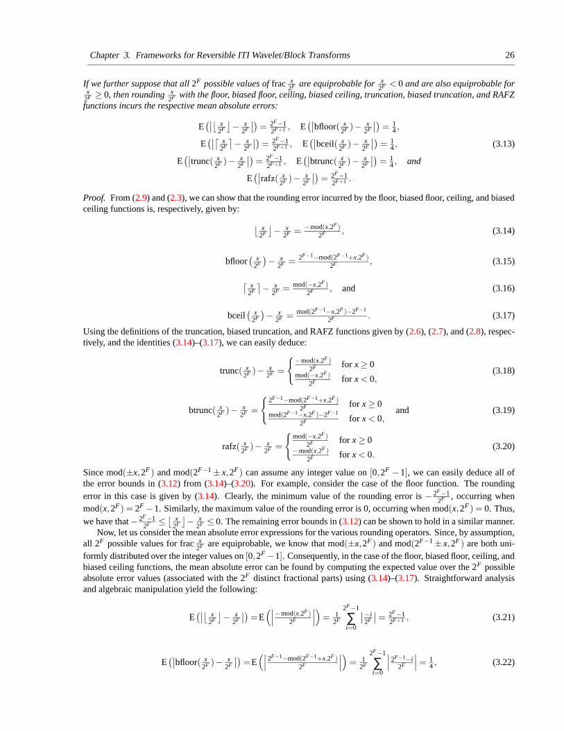
Chapter 3. Frameworks for Reversible ITI Wavelet/Block Transforms 26
If we further suppose that all 2F possible values of frac x2F are equiprobable for x
2F < 0 and are also equiprobable forx
2F ≥ 0, then rounding x2F with the floor, biased floor, ceiling, biased ceiling, truncation, biased truncation, and RAFZ
functions incurs the respective mean absolute errors:
E(∣∣⌊
x2F
⌋− x
2F
∣∣)
= 2F−12F+1 , E
(∣∣bfloor( x
2F )− x2F
∣∣)
= 14 ,
E(∣∣⌈
x2F
⌉− x
2F
∣∣)
= 2F−12F+1 , E
(∣∣bceil( x
2F )− x2F
∣∣)
= 14 , (3.13)
E(∣∣trunc( x
2F )− x2F
∣∣)
= 2F−12F+1 , E
(∣∣btrunc( x
2F )− x2F
∣∣)
= 14 , and
E(∣∣rafz( x
2F )− x2F
∣∣)
= 2F−12F+1 .
Proof. From (2.9) and (2.3), we can show that the rounding error incurred by the floor, biased floor, ceiling, and biasedceiling functions is, respectively, given by:
⌊x
2F
⌋− x
2F = −mod(x,2F )2F , (3.14)
bfloor(
x2F
)− x
2F = 2F−1−mod(2F−1+x,2F )2F , (3.15)
⌈x
2F
⌉− x
2F = mod(−x,2F )2F , and (3.16)
bceil(
x2F
)− x
2F = mod(2F−1−x,2F )−2F−1
2F . (3.17)
Using the definitions of the truncation, biased truncation, and RAFZ functions given by (2.6), (2.7), and (2.8), respec-tively, and the identities (3.14)–(3.17), we can easily deduce:
trunc( x2F )− x
2F =
{−mod(x,2F )2F for x ≥ 0
mod(−x,2F )2F for x < 0,
(3.18)
btrunc( x2F )− x
2F =
{2F−1−mod(2F−1+x,2F )
2F for x ≥ 0mod(2F−1−x,2F )−2F−1
2F for x < 0,and (3.19)
rafz( x2F )− x
2F =
{mod(−x,2F )
2F for x ≥ 0−mod(x,2F )
2F for x < 0.(3.20)
Since mod(±x,2F) and mod(2F−1 ± x,2F) can assume any integer value on [0,2F − 1], we can easily deduce all ofthe error bounds in (3.12) from (3.14)–(3.20). For example, consider the case of the floor function. The roundingerror in this case is given by (3.14). Clearly, the minimum value of the rounding error is − 2F−1
2F , occurring whenmod(x,2F) = 2F −1. Similarly, the maximum value of the rounding error is 0, occurring when mod(x,2F) = 0. Thus,
we have that − 2F−12F ≤
⌊x
2F
⌋− x
2F ≤ 0. The remaining error bounds in (3.12) can be shown to hold in a similar manner.Now, let us consider the mean absolute error expressions for the various rounding operators. Since, by assumption,
all 2F possible values for frac x2F are equiprobable, we know that mod(±x,2F) and mod(2F−1 ± x,2F) are both uni-
formly distributed over the integer values on [0,2F −1]. Consequently, in the case of the floor, biased floor, ceiling, andbiased ceiling functions, the mean absolute error can be found by computing the expected value over the 2F possibleabsolute error values (associated with the 2F distinct fractional parts) using (3.14)–(3.17). Straightforward analysisand algebraic manipulation yield the following:
E(∣∣⌊
x2F
⌋− x
2F
∣∣)
=E(∣∣∣−mod(x,2F )
2F
∣∣∣
)
= 12F
2F−1
∑i=0
∣∣−i
2F
∣∣= 2F−1
2F+1 , (3.21)
E(∣∣bfloor( x
2F )− x2F
∣∣)
=E(∣∣∣
2F−1−mod(2F−1+x,2F )2F
∣∣∣
)
= 12F
2F−1
∑i=0
∣∣∣
2F−1−i2F
∣∣∣= 1
4 , (3.22)
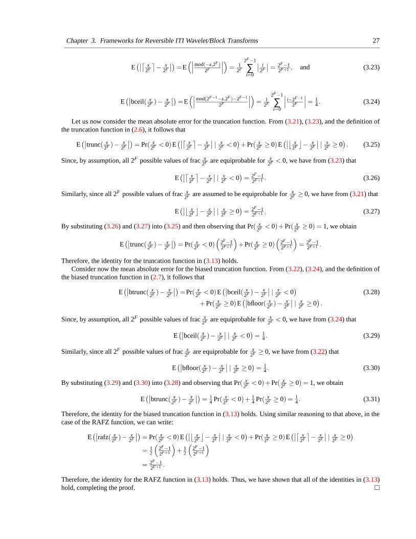
Chapter 3. Frameworks for Reversible ITI Wavelet/Block Transforms 27
E(∣∣⌈
x2F
⌉− x
2F
∣∣)
=E(∣∣∣
mod(−x,2F )2F
∣∣∣
)
= 12F
2F−1
∑i=0
∣∣ i
2F
∣∣= 2F−1
2F+1 , and (3.23)
E(∣∣bceil( x
2F )− x2F
∣∣)
=E(∣∣∣
mod(2F−1−x,2F )−2F−1
2F
∣∣∣
)
= 12F
2F−1
∑i=0
∣∣∣
i−2F−1
2F
∣∣∣= 1
4 . (3.24)
Let us now consider the mean absolute error for the truncation function. From (3.21), (3.23), and the definition ofthe truncation function in (2.6), it follows that
E(∣∣trunc( x
2F )− x2F
∣∣)
= Pr( x2F < 0)E
(∣∣⌈
x2F
⌉− x
2F
∣∣ | x
2F < 0)+Pr( x
2F ≥ 0)E(∣∣⌊
x2F
⌋− x
2F
∣∣ | x
2F ≥ 0). (3.25)
Since, by assumption, all 2F possible values of frac x2F are equiprobable for x
2F < 0, we have from (3.23) that
E(∣∣⌈
x2F
⌉− x
2F
∣∣ | x
2F < 0)
= 2F−12F+1 . (3.26)
Similarly, since all 2F possible values of frac x2F are assumed to be equiprobable for x
2F ≥ 0, we have from (3.21) that
E(∣∣⌊
x2F
⌋− x
2F
∣∣ | x
2F ≥ 0)
= 2F−12F+1 . (3.27)
By substituting (3.26) and (3.27) into (3.25) and then observing that Pr( x2F < 0)+Pr( x
2F ≥ 0) = 1, we obtain
E(∣∣trunc( x
2F )− x2F
∣∣)
= Pr( x2F < 0)
(2F−12F+1
)
+Pr( x2F ≥ 0)
(2F−12F+1
)
= 2F−12F+1 .
Therefore, the identity for the truncation function in (3.13) holds.Consider now the mean absolute error for the biased truncation function. From (3.22), (3.24), and the definition of
the biased truncation function in (2.7), it follows that
E(∣∣btrunc( x
2F )− x2F
∣∣)
=Pr( x2F < 0)E
(∣∣bceil( x
2F )− x2F
∣∣ | x
2F < 0)
(3.28)
+Pr( x2F ≥ 0)E
(∣∣bfloor( x
2F )− x2F
∣∣ | x
2F ≥ 0).
Since, by assumption, all 2F possible values of frac x2F are equiprobable for x
2F < 0, we have from (3.24) that
E(∣∣bceil( x
2F )− x2F
∣∣ | x
2F < 0)
= 14 . (3.29)
Similarly, since all 2F possible values of frac x2F are equiprobable for x
2F ≥ 0, we have from (3.22) that
E(∣∣bfloor( x
2F )− x2F
∣∣ | x
2F ≥ 0)
= 14 . (3.30)
By substituting (3.29) and (3.30) into (3.28) and observing that Pr( x2F < 0)+Pr( x
2F ≥ 0) = 1, we obtain
E(∣∣btrunc( x
2F )− x2F
∣∣)
= 14 Pr( x
2F < 0)+ 14 Pr( x
2F ≥ 0) = 14 . (3.31)
Therefore, the identity for the biased truncation function in (3.13) holds. Using similar reasoning to that above, in thecase of the RAFZ function, we can write:
E(∣∣rafz( x
2F )− x2F
∣∣)
= Pr( x2F < 0)E
(∣∣⌊
x2F
⌋− x
2F
∣∣ | x
2F < 0)+Pr( x
2F ≥ 0)E(∣∣⌈
x2F
⌉− x
2F
∣∣ | x
2F ≥ 0)
= 12
(2F−12F+1
)
+ 12
(2F−12F+1
)
= 2F−12F+1 .
Therefore, the identity for the RAFZ function in (3.13) holds. Thus, we have shown that all of the identities in (3.13)hold, completing the proof.
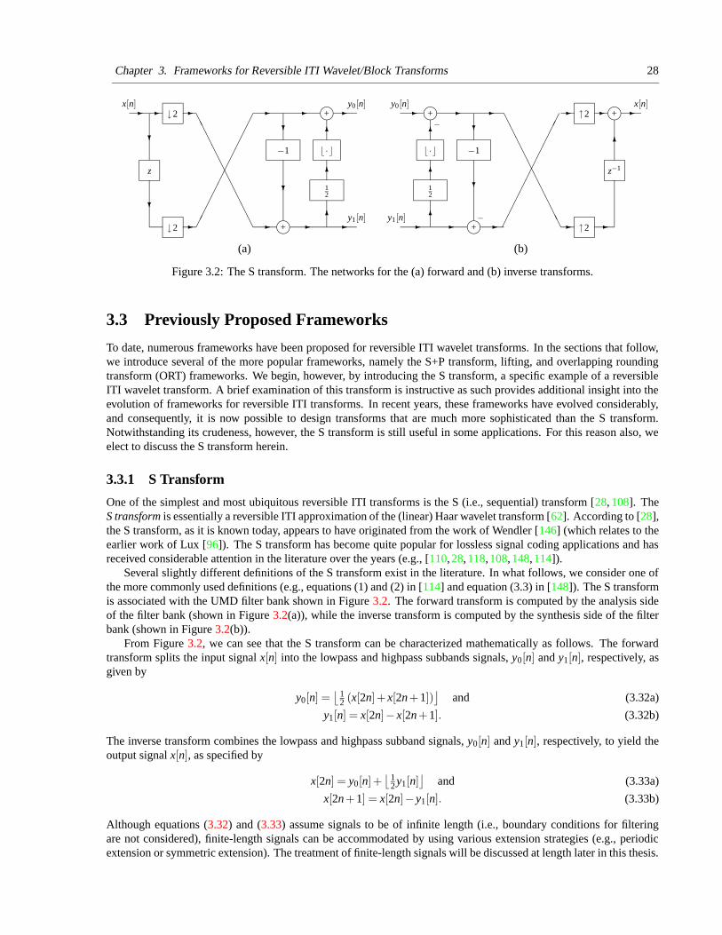
Chapter 3. Frameworks for Reversible ITI Wavelet/Block Transforms 28
j+
j+↓2
↓2
z
��
��
��
��
�� A
AA
AA
AA
AA
A
12
b ·c−1
6?
?
- - -
-
- -
6
6
-
?
?-
--
x[n] y0[n]
y1[n]
(a)
j+
j+ ↑2
↑2 j+
z−1
AAAAAAAAAA�
���������
b ·c
12
−1
6
6
6
-
-
6?
?
- -
- -
- -
--
- x[n]
−
−y1[n]
y0[n]
(b)
Figure 3.2: The S transform. The networks for the (a) forward and (b) inverse transforms.
3.3 Previously Proposed Frameworks
To date, numerous frameworks have been proposed for reversible ITI wavelet transforms. In the sections that follow,we introduce several of the more popular frameworks, namely the S+P transform, lifting, and overlapping roundingtransform (ORT) frameworks. We begin, however, by introducing the S transform, a specific example of a reversibleITI wavelet transform. A brief examination of this transform is instructive as such provides additional insight into theevolution of frameworks for reversible ITI transforms. In recent years, these frameworks have evolved considerably,and consequently, it is now possible to design transforms that are much more sophisticated than the S transform.Notwithstanding its crudeness, however, the S transform is still useful in some applications. For this reason also, weelect to discuss the S transform herein.
3.3.1 S Transform
One of the simplest and most ubiquitous reversible ITI transforms is the S (i.e., sequential) transform [28, 108]. TheS transform is essentially a reversible ITI approximation of the (linear) Haar wavelet transform [62]. According to [28],the S transform, as it is known today, appears to have originated from the work of Wendler [146] (which relates to theearlier work of Lux [96]). The S transform has become quite popular for lossless signal coding applications and hasreceived considerable attention in the literature over the years (e.g., [110, 28, 118, 108, 148, 114]).
Several slightly different definitions of the S transform exist in the literature. In what follows, we consider one ofthe more commonly used definitions (e.g., equations (1) and (2) in [114] and equation (3.3) in [148]). The S transformis associated with the UMD filter bank shown in Figure 3.2. The forward transform is computed by the analysis sideof the filter bank (shown in Figure 3.2(a)), while the inverse transform is computed by the synthesis side of the filterbank (shown in Figure 3.2(b)).
From Figure 3.2, we can see that the S transform can be characterized mathematically as follows. The forwardtransform splits the input signal x[n] into the lowpass and highpass subbands signals, y0[n] and y1[n], respectively, asgiven by
y0[n] =⌊
12 (x[2n]+ x[2n+1])
⌋and (3.32a)
y1[n] = x[2n]− x[2n+1]. (3.32b)
The inverse transform combines the lowpass and highpass subband signals, y0[n] and y1[n], respectively, to yield theoutput signal x[n], as specified by
x[2n] = y0[n]+⌊
12 y1[n]
⌋and (3.33a)
x[2n+1] = x[2n]− y1[n]. (3.33b)
Although equations (3.32) and (3.33) assume signals to be of infinite length (i.e., boundary conditions for filteringare not considered), finite-length signals can be accommodated by using various extension strategies (e.g., periodicextension or symmetric extension). The treatment of finite-length signals will be discussed at length later in this thesis.
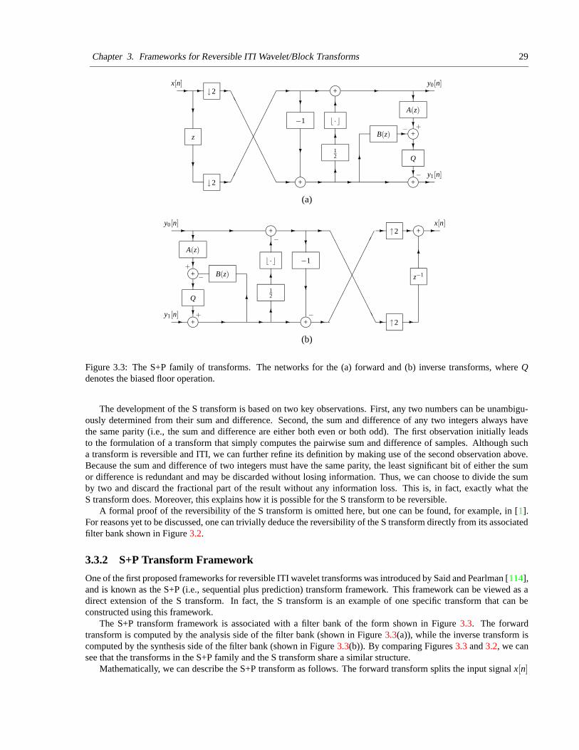
Chapter 3. Frameworks for Reversible ITI Wavelet/Block Transforms 29
j+
j+
j+
j+↓2
↓2
z
��
��
��
��
�� A
AA
AA
AA
AA
AA(z)
B(z)
12
b ·c
Q
−1
6?
?
- - -
-
- - -
6
6
6
-
-
-
-
?
?
?
?
?
?
- - -
− +
y1[n]
y0[n]x[n]
−
(a)
j+
j+
j+ ↑2
↑2 j+
z−1
j+
AAAAAAAAAA�
���������
Q
A(z)
B(z)
b ·c
12
−1
6
6
6
-
--?
?
6
-
- - -
- -
- -
---?
?
?
?6
x[n]y0[n]
y1[n] −
+
−
−
+
(b)
Figure 3.3: The S+P family of transforms. The networks for the (a) forward and (b) inverse transforms, where Qdenotes the biased floor operation.
The development of the S transform is based on two key observations. First, any two numbers can be unambigu-ously determined from their sum and difference. Second, the sum and difference of any two integers always havethe same parity (i.e., the sum and difference are either both even or both odd). The first observation initially leadsto the formulation of a transform that simply computes the pairwise sum and difference of samples. Although sucha transform is reversible and ITI, we can further refine its definition by making use of the second observation above.Because the sum and difference of two integers must have the same parity, the least significant bit of either the sumor difference is redundant and may be discarded without losing information. Thus, we can choose to divide the sumby two and discard the fractional part of the result without any information loss. This is, in fact, exactly what theS transform does. Moreover, this explains how it is possible for the S transform to be reversible.
A formal proof of the reversibility of the S transform is omitted here, but one can be found, for example, in [1].For reasons yet to be discussed, one can trivially deduce the reversibility of the S transform directly from its associatedfilter bank shown in Figure 3.2.
3.3.2 S+P Transform Framework
One of the first proposed frameworks for reversible ITI wavelet transforms was introduced by Said and Pearlman [114],and is known as the S+P (i.e., sequential plus prediction) transform framework. This framework can be viewed as adirect extension of the S transform. In fact, the S transform is an example of one specific transform that can beconstructed using this framework.
The S+P transform framework is associated with a filter bank of the form shown in Figure 3.3. The forwardtransform is computed by the analysis side of the filter bank (shown in Figure 3.3(a)), while the inverse transform iscomputed by the synthesis side of the filter bank (shown in Figure 3.3(b)). By comparing Figures 3.3 and 3.2, we cansee that the transforms in the S+P family and the S transform share a similar structure.
Mathematically, we can describe the S+P transform as follows. The forward transform splits the input signal x[n]
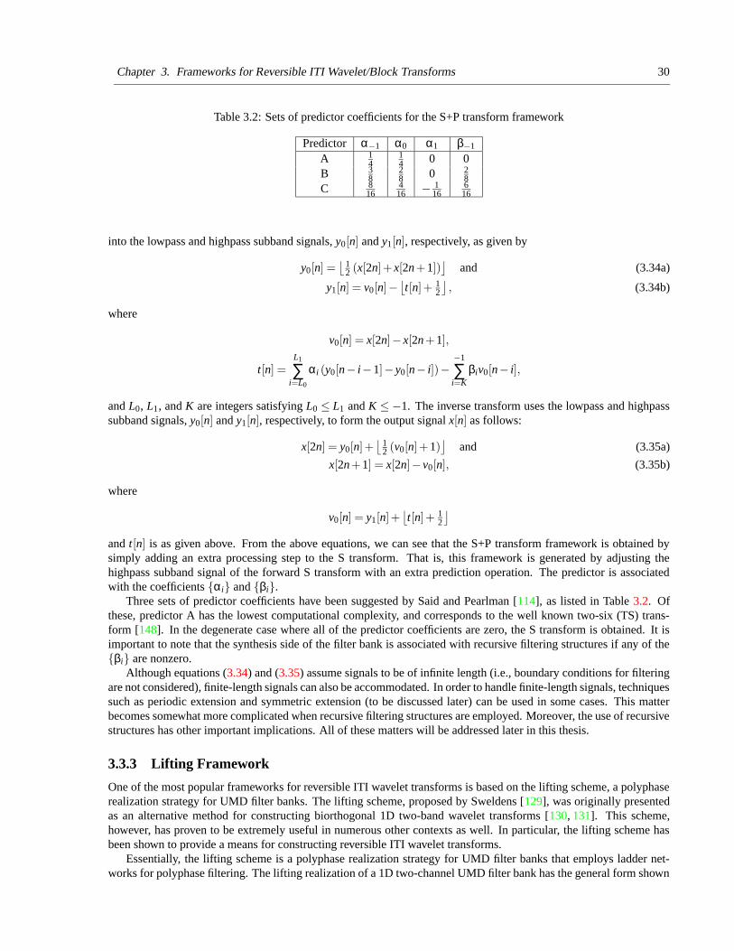
Chapter 3. Frameworks for Reversible ITI Wavelet/Block Transforms 30
Table 3.2: Sets of predictor coefficients for the S+P transform framework
Predictor α−1 α0 α1 β−1
A 14
14 0 0
B 38
28 0 2
8C 8
164
16 − 116
616
into the lowpass and highpass subband signals, y0[n] and y1[n], respectively, as given by
y0[n] =⌊
12 (x[2n]+ x[2n+1])
⌋and (3.34a)
y1[n] = v0[n]−⌊t[n]+ 1
2
⌋, (3.34b)
where
v0[n] = x[2n]− x[2n+1],
t[n] =L1
∑i=L0
αi (y0[n− i−1]− y0[n− i])−−1
∑i=K
βiv0[n− i],
and L0, L1, and K are integers satisfying L0 ≤ L1 and K ≤ −1. The inverse transform uses the lowpass and highpasssubband signals, y0[n] and y1[n], respectively, to form the output signal x[n] as follows:
x[2n] = y0[n]+⌊
12 (v0[n]+1)
⌋and (3.35a)
x[2n+1] = x[2n]− v0[n], (3.35b)
where
v0[n] = y1[n]+⌊t[n]+ 1
2
⌋
and t[n] is as given above. From the above equations, we can see that the S+P transform framework is obtained bysimply adding an extra processing step to the S transform. That is, this framework is generated by adjusting thehighpass subband signal of the forward S transform with an extra prediction operation. The predictor is associatedwith the coefficients {αi} and {βi}.
Three sets of predictor coefficients have been suggested by Said and Pearlman [114], as listed in Table 3.2. Ofthese, predictor A has the lowest computational complexity, and corresponds to the well known two-six (TS) trans-form [148]. In the degenerate case where all of the predictor coefficients are zero, the S transform is obtained. It isimportant to note that the synthesis side of the filter bank is associated with recursive filtering structures if any of the{βi} are nonzero.
Although equations (3.34) and (3.35) assume signals to be of infinite length (i.e., boundary conditions for filteringare not considered), finite-length signals can also be accommodated. In order to handle finite-length signals, techniquessuch as periodic extension and symmetric extension (to be discussed later) can be used in some cases. This matterbecomes somewhat more complicated when recursive filtering structures are employed. Moreover, the use of recursivestructures has other important implications. All of these matters will be addressed later in this thesis.
3.3.3 Lifting Framework
One of the most popular frameworks for reversible ITI wavelet transforms is based on the lifting scheme, a polyphaserealization strategy for UMD filter banks. The lifting scheme, proposed by Sweldens [129], was originally presentedas an alternative method for constructing biorthogonal 1D two-band wavelet transforms [130, 131]. This scheme,however, has proven to be extremely useful in numerous other contexts as well. In particular, the lifting scheme hasbeen shown to provide a means for constructing reversible ITI wavelet transforms.
Essentially, the lifting scheme is a polyphase realization strategy for UMD filter banks that employs ladder net-works for polyphase filtering. The lifting realization of a 1D two-channel UMD filter bank has the general form shown
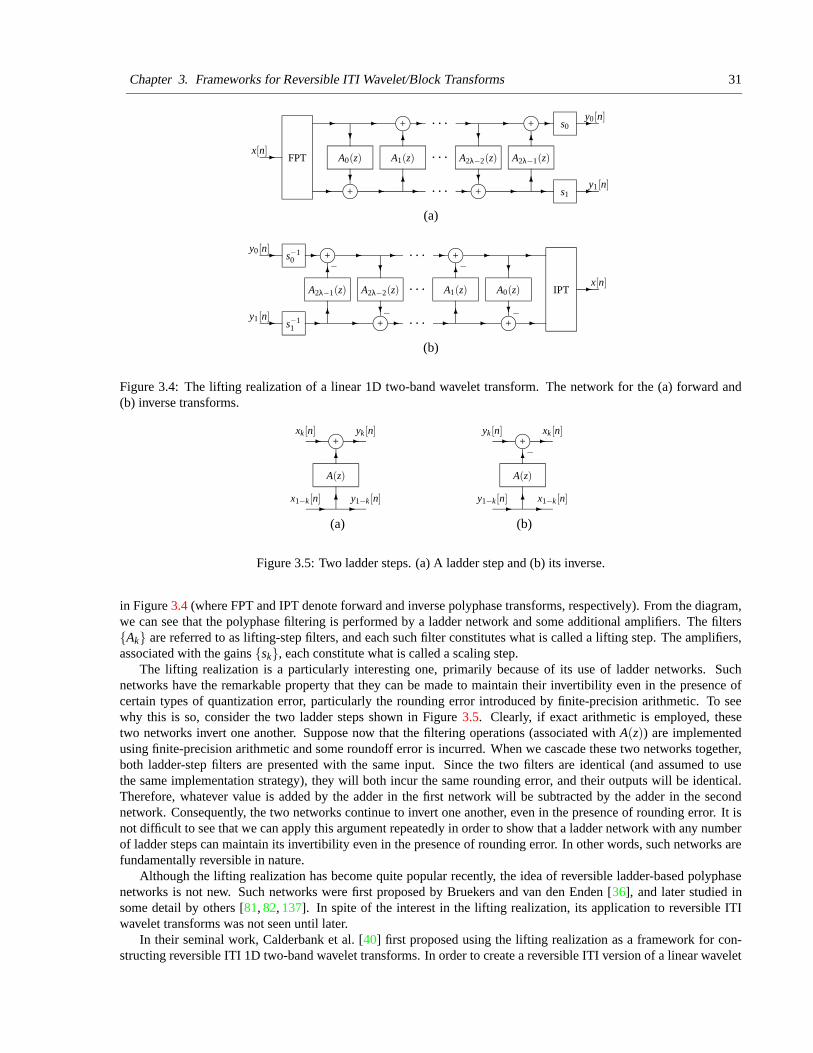
Chapter 3. Frameworks for Reversible ITI Wavelet/Block Transforms 31
j+
j+ j+
j+
A0(z) A1(z)FPT
?
?6
6
-
- -
-
6?
-?
-
- -
6- -
--
-
-
-
· · ·
· · ·
· · ·
A2λ−2(z) A2λ−1(z)
s0
s1
y0[n]
y1[n]
x[n]
(a)
j+
j+
j+
j+
A1(z) A0(z)
s−10
s−11
IPT
?6
6?-
-
6
6
?
?- -
---
---
- -
-
-
-
A2λ−2(z)
−
A2λ−1(z)
− · · ·
· · ·
· · ·−
−
y0[n]
y1[n]
x[n]
(b)
Figure 3.4: The lifting realization of a linear 1D two-band wavelet transform. The network for the (a) forward and(b) inverse transforms.
j+
A(z)6
6- -
- -
x1−k[n] y1−k[n]
yk[n]xk[n]
(a)
j+
A(z)6
6- -
- -−
y1−k[n] x1−k[n]
xk[n]yk[n]
(b)
Figure 3.5: Two ladder steps. (a) A ladder step and (b) its inverse.
in Figure 3.4 (where FPT and IPT denote forward and inverse polyphase transforms, respectively). From the diagram,we can see that the polyphase filtering is performed by a ladder network and some additional amplifiers. The filters{Ak} are referred to as lifting-step filters, and each such filter constitutes what is called a lifting step. The amplifiers,associated with the gains {sk}, each constitute what is called a scaling step.
The lifting realization is a particularly interesting one, primarily because of its use of ladder networks. Suchnetworks have the remarkable property that they can be made to maintain their invertibility even in the presence ofcertain types of quantization error, particularly the rounding error introduced by finite-precision arithmetic. To seewhy this is so, consider the two ladder steps shown in Figure 3.5. Clearly, if exact arithmetic is employed, thesetwo networks invert one another. Suppose now that the filtering operations (associated with A(z)) are implementedusing finite-precision arithmetic and some roundoff error is incurred. When we cascade these two networks together,both ladder-step filters are presented with the same input. Since the two filters are identical (and assumed to usethe same implementation strategy), they will both incur the same rounding error, and their outputs will be identical.Therefore, whatever value is added by the adder in the first network will be subtracted by the adder in the secondnetwork. Consequently, the two networks continue to invert one another, even in the presence of rounding error. It isnot difficult to see that we can apply this argument repeatedly in order to show that a ladder network with any numberof ladder steps can maintain its invertibility even in the presence of rounding error. In other words, such networks arefundamentally reversible in nature.
Although the lifting realization has become quite popular recently, the idea of reversible ladder-based polyphasenetworks is not new. Such networks were first proposed by Bruekers and van den Enden [36], and later studied insome detail by others [81, 82, 137]. In spite of the interest in the lifting realization, its application to reversible ITIwavelet transforms was not seen until later.
In their seminal work, Calderbank et al. [40] first proposed using the lifting realization as a framework for con-structing reversible ITI 1D two-band wavelet transforms. In order to create a reversible ITI version of a linear wavelet
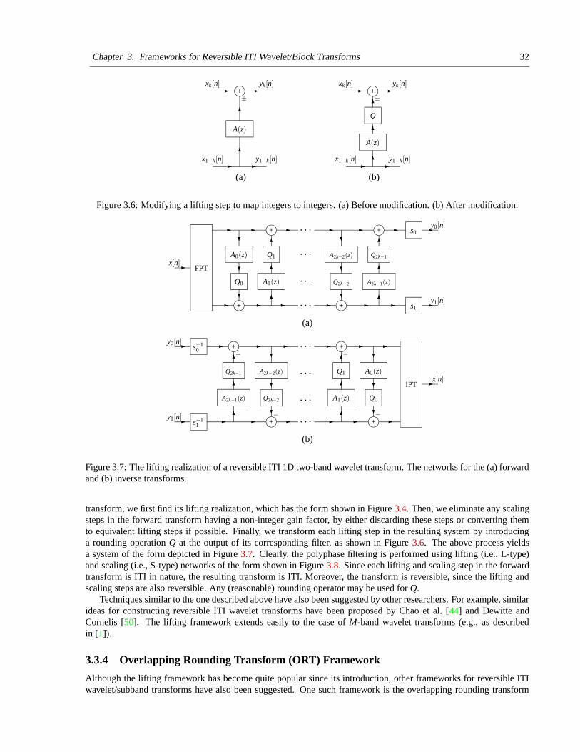
Chapter 3. Frameworks for Reversible ITI Wavelet/Block Transforms 32
j+
A(z)
- -
- -
6
6
±
y1−k[n]
xk[n] yk[n]
x1−k[n]
(a)
j+
Q
A(z)
- -6
6
-
6
-±
y1−k[n]
xk[n] yk[n]
x1−k[n]
(b)
Figure 3.6: Modifying a lifting step to map integers to integers. (a) Before modification. (b) After modification.
j+
j+
j+
j+
A0(z)
Q0
Q1
A1(z)
s0
s1
FPT
6
6
6?
?
?
-
-
--
- - 6
6
6
- -
-
?
?
?-
-
-
-
-
-
· · ·
· · ·
· · ·
· · ·
Q2λ−2
Q2λ−1
A2λ−1(z)
A2λ−2(z)
y1[n]
y0[n]
x[n]
(a)
j+
j+
j+
j+
s−10
s−11
A0(z)Q1
A1(z) Q0
IPT
?- - -
- 6?
-- - - -6
- -
6?
-
6
?
6 6? ?
-
-
-Q2λ−1 A2λ−2(z)
A2λ−1(z) Q2λ−2 · · ·
· · ·
· · ·
· · ·− −
− −
y1[n]
y0[n]
x[n]
(b)
Figure 3.7: The lifting realization of a reversible ITI 1D two-band wavelet transform. The networks for the (a) forwardand (b) inverse transforms.
transform, we first find its lifting realization, which has the form shown in Figure 3.4. Then, we eliminate any scalingsteps in the forward transform having a non-integer gain factor, by either discarding these steps or converting themto equivalent lifting steps if possible. Finally, we transform each lifting step in the resulting system by introducinga rounding operation Q at the output of its corresponding filter, as shown in Figure 3.6. The above process yieldsa system of the form depicted in Figure 3.7. Clearly, the polyphase filtering is performed using lifting (i.e., L-type)and scaling (i.e., S-type) networks of the form shown in Figure 3.8. Since each lifting and scaling step in the forwardtransform is ITI in nature, the resulting transform is ITI. Moreover, the transform is reversible, since the lifting andscaling steps are also reversible. Any (reasonable) rounding operator may be used for Q.
Techniques similar to the one described above have also been suggested by other researchers. For example, similarideas for constructing reversible ITI wavelet transforms have been proposed by Chao et al. [44] and Dewitte andCornelis [50]. The lifting framework extends easily to the case of M-band wavelet transforms (e.g., as describedin [1]).
3.3.4 Overlapping Rounding Transform (ORT) Framework
Although the lifting framework has become quite popular since its introduction, other frameworks for reversible ITIwavelet/subband transforms have also been suggested. One such framework is the overlapping rounding transform
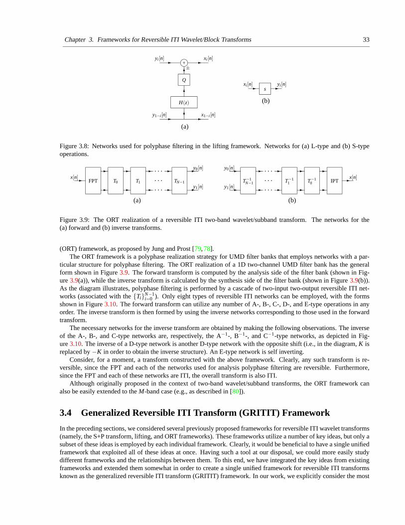
Chapter 3. Frameworks for Reversible ITI Wavelet/Block Transforms 33
Q
H(z)
j+
6
- -
-
6
6
-
y1−i[n] x1−i[n]
xi[n]yi[n]
±
(a)
-- yi[n]xi[n]s
(b)
Figure 3.8: Networks used for polyphase filtering in the lifting framework. Networks for (a) L-type and (b) S-typeoperations.
--
- -
- -
- -
- -
-FPT T0 T1
x[n]· · ·
TN−1
y0[n]
y1[n]· · ·· · ·
(a)
--
--
--
--
--
- · · ·T−1
N−1 T−11 T−1
0 IPTx[n]
y0[n]
y1[n]
· · ·· · ·
(b)
Figure 3.9: The ORT realization of a reversible ITI two-band wavelet/subband transform. The networks for the(a) forward and (b) inverse transforms.
(ORT) framework, as proposed by Jung and Prost [79, 78].The ORT framework is a polyphase realization strategy for UMD filter banks that employs networks with a par-
ticular structure for polyphase filtering. The ORT realization of a 1D two-channel UMD filter bank has the generalform shown in Figure 3.9. The forward transform is computed by the analysis side of the filter bank (shown in Fig-ure 3.9(a)), while the inverse transform is calculated by the synthesis side of the filter bank (shown in Figure 3.9(b)).As the diagram illustrates, polyphase filtering is performed by a cascade of two-input two-output reversible ITI net-works (associated with the {Ti}N−1
i=0 ). Only eight types of reversible ITI networks can be employed, with the formsshown in Figure 3.10. The forward transform can utilize any number of A-, B-, C-, D-, and E-type operations in anyorder. The inverse transform is then formed by using the inverse networks corresponding to those used in the forwardtransform.
The necessary networks for the inverse transform are obtained by making the following observations. The inverseof the A-, B-, and C-type networks are, respectively, the A−1-, B−1-, and C−1-type networks, as depicted in Fig-ure 3.10. The inverse of a D-type network is another D-type network with the opposite shift (i.e., in the diagram, K isreplaced by −K in order to obtain the inverse structure). An E-type network is self inverting.
Consider, for a moment, a transform constructed with the above framework. Clearly, any such transform is re-versible, since the FPT and each of the networks used for analysis polyphase filtering are reversible. Furthermore,since the FPT and each of these networks are ITI, the overall transform is also ITI.
Although originally proposed in the context of two-band wavelet/subband transforms, the ORT framework canalso be easily extended to the M-band case (e.g., as described in [80]).
3.4 Generalized Reversible ITI Transform (GRITIT) Framework
In the preceding sections, we considered several previously proposed frameworks for reversible ITI wavelet transforms(namely, the S+P transform, lifting, and ORT frameworks). These frameworks utilize a number of key ideas, but only asubset of these ideas is employed by each individual framework. Clearly, it would be beneficial to have a single unifiedframework that exploited all of these ideas at once. Having such a tool at our disposal, we could more easily studydifferent frameworks and the relationships between them. To this end, we have integrated the key ideas from existingframeworks and extended them somewhat in order to create a single unified framework for reversible ITI transformsknown as the generalized reversible ITI transform (GRITIT) framework. In our work, we explicitly consider the most
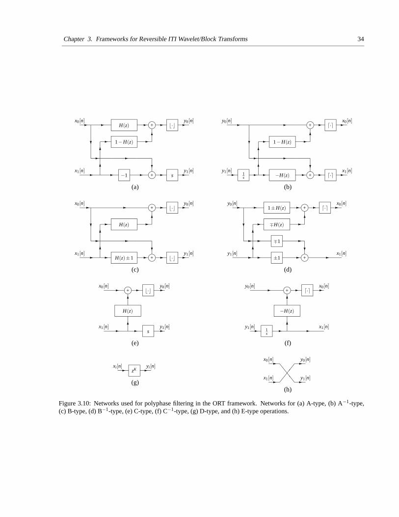
Chapter 3. Frameworks for Reversible ITI Wavelet/Block Transforms 34
H(z) j+
j+ s
b·c
−1
-
6
- -?
-6
-
?
6
--
--
-
-
-
- - y1[n]
y0[n]
1−H(z)
x1[n]
x0[n]
(a)
j+
j+1s −H(z)
1−H(z)
-
----6
- -?
-6
?
6
--
--
-
-
d·ey0[n] x0[n]
x1[n]y1[n]d·e
(b)
j+
j+
b·c
b·c--6
- -?
-6
?
6
--
---
- -
-
y1[n]
y0[n]x0[n]
x1[n]H(z)±1
H(z)
(c)
j+
j+
-
-
---6
- -?
-6
-
?-
6
---
- x1[n]
x0[n]
∓H(z)
1±H(z) d·e
y1[n]
y0[n]
∓1
±1
(d)
j+ b·c
H(z)
s
-
6
-
-
-6-
- y0[n]
y1[n]
x0[n]
x1[n]
(e)
j+ -
-
6
- -
6- -
−H(z)
d·e
1s
y1[n]
y0[n] x0[n]
x1[n]
(f)
-- yi[n]xi[n]zK
(g)
\\
\��
�-
-
-
-
x0[n]
x1[n]
y0[n]
y1[n]
(h)
Figure 3.10: Networks used for polyphase filtering in the ORT framework. Networks for (a) A-type, (b) A−1-type,(c) B-type, (d) B−1-type, (e) C-type, (f) C−1-type, (g) D-type, and (h) E-type operations.
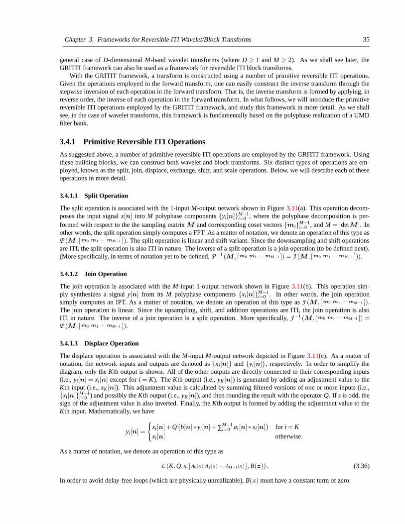
Chapter 3. Frameworks for Reversible ITI Wavelet/Block Transforms 35
general case of D-dimensional M-band wavelet transforms (where D ≥ 1 and M ≥ 2). As we shall see later, theGRITIT framework can also be used as a framework for reversible ITI block transforms.
With the GRITIT framework, a transform is constructed using a number of primitive reversible ITI operations.Given the operations employed in the forward transform, one can easily construct the inverse transform through thestepwise inversion of each operation in the forward transform. That is, the inverse transform is formed by applying, inreverse order, the inverse of each operation in the forward transform. In what follows, we will introduce the primitivereversible ITI operations employed by the GRITIT framework, and study this framework in more detail. As we shallsee, in the case of wavelet transforms, this framework is fundamentally based on the polyphase realization of a UMDfilter bank.
3.4.1 Primitive Reversible ITI Operations
As suggested above, a number of primitive reversible ITI operations are employed by the GRITIT framework. Usingthese building blocks, we can construct both wavelet and block transforms. Six distinct types of operations are em-ployed, known as the split, join, displace, exchange, shift, and scale operations. Below, we will describe each of theseoperations in more detail.
3.4.1.1 Split Operation
The split operation is associated with the 1-input M-output network shown in Figure 3.11(a). This operation decom-poses the input signal x[n] into M polyphase components {yi[n]}M−1
i=0 , where the polyphase decomposition is per-formed with respect to the the sampling matrix M and corresponding coset vectors {mi}M−1
i=0 , and M = |detM |. Inother words, the split operation simply computes a FPT. As a matter of notation, we denote an operation of this type asP (M , [m0 m1 ··· mM−1 ]). The split operation is linear and shift variant. Since the downsampling and shift operationsare ITI, the split operation is also ITI in nature. The inverse of a split operation is a join operation (to be defined next).(More specifically, in terms of notation yet to be defined, P −1 (M , [m0 m1 ··· mM−1 ]) = J (M , [m0 m1 ··· mM−1 ])).
3.4.1.2 Join Operation
The join operation is associated with the M-input 1-output network shown in Figure 3.11(b). This operation sim-ply synthesizes a signal y[n] from its M polyphase components {xi[n]}M−1
i=0 . In other words, the join operationsimply computes an IPT. As a matter of notation, we denote an operation of this type as J (M , [ m0 m1 ··· mM−1 ]).The join operation is linear. Since the upsampling, shift, and addition operations are ITI, the join operation is alsoITI in nature. The inverse of a join operation is a split operation. More specifically, J −1 (M , [m0 m1 ··· mM−1 ]) =P (M , [m0 m1 ··· mM−1 ]).
3.4.1.3 Displace Operation
The displace operation is associated with the M-input M-output network depicted in Figure 3.11(c). As a matter ofnotation, the network inputs and outputs are denoted as {xi[n]} and {yi[n]}, respectively. In order to simplify thediagram, only the Kth output is shown. All of the other outputs are directly connected to their corresponding inputs(i.e., yi[n] = xi[n] except for i = K). The Kth output (i.e., yK [n]) is generated by adding an adjustment value to theKth input (i.e., xK [n]). This adjustment value is calculated by summing filtered versions of one or more inputs (i.e.,{xi[n]}M−1
i=0 ) and possibly the Kth output (i.e., yK [n]), and then rounding the result with the operator Q. If s is odd, thesign of the adjustment value is also inverted. Finally, the Kth output is formed by adding the adjustment value to theKth input. Mathematically, we have
yi[n] =
{
xi[n]+Q(b[n]∗ yi[n]+∑M−1
l=0 al [n]∗ xl [n])
for i = K
xi[n] otherwise.
As a matter of notation, we denote an operation of this type as
L (K,Q,s, [A0(z) A1(z) ··· AM−1(z) ] ,B(z)) . (3.36)
In order to avoid delay-free loops (which are physically unrealizable), B(z) must have a constant term of zero.
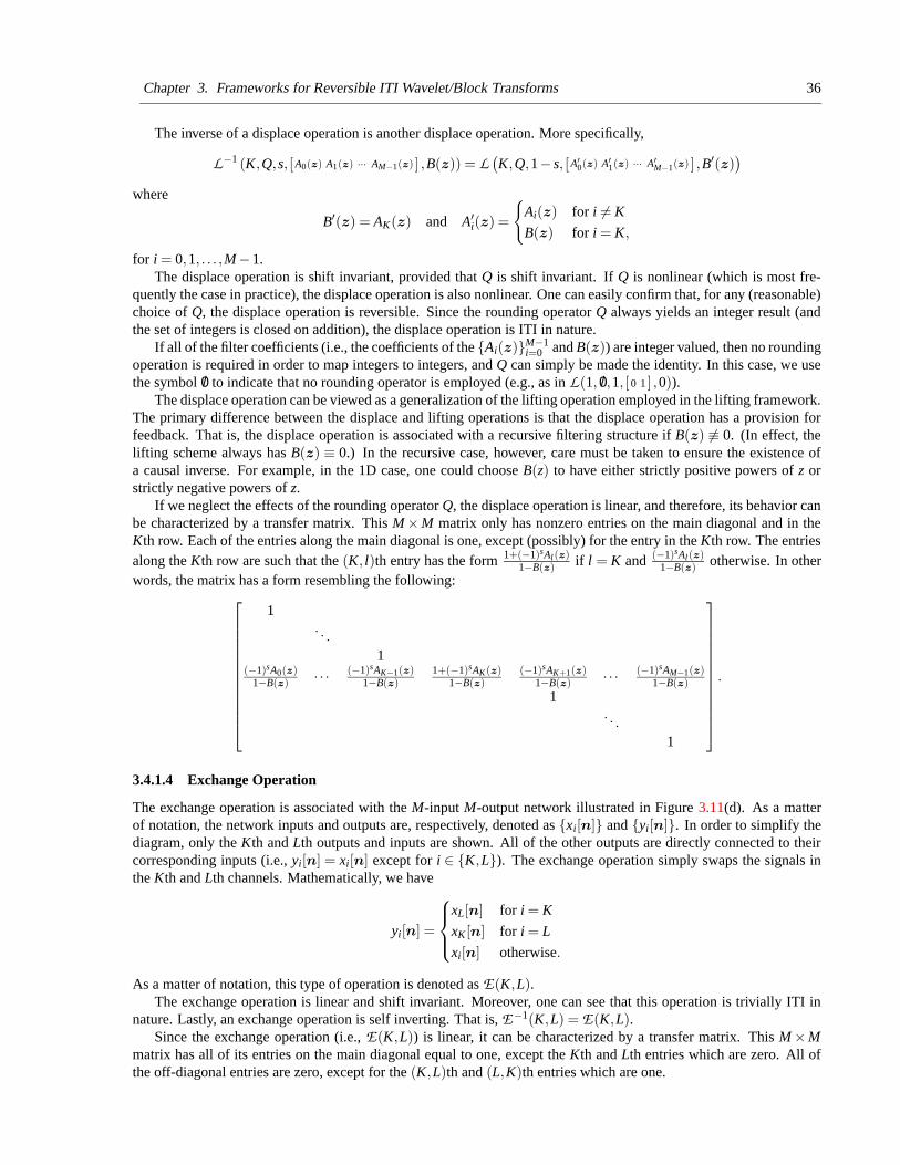
Chapter 3. Frameworks for Reversible ITI Wavelet/Block Transforms 36
The inverse of a displace operation is another displace operation. More specifically,
L−1 (K,Q,s, [A0(z) A1(z) ··· AM−1(z) ] ,B(z)) = L(K,Q,1− s, [A′
0(z) A′1(z) ··· A′
M−1(z) ] ,B′(z))
where
B′(z) = AK(z) and A′i(z) =
{
Ai(z) for i 6= K
B(z) for i = K,
for i = 0,1, . . . ,M−1.The displace operation is shift invariant, provided that Q is shift invariant. If Q is nonlinear (which is most fre-
quently the case in practice), the displace operation is also nonlinear. One can easily confirm that, for any (reasonable)choice of Q, the displace operation is reversible. Since the rounding operator Q always yields an integer result (andthe set of integers is closed on addition), the displace operation is ITI in nature.
If all of the filter coefficients (i.e., the coefficients of the {Ai(z)}M−1i=0 and B(z)) are integer valued, then no rounding
operation is required in order to map integers to integers, and Q can simply be made the identity. In this case, we usethe symbol /0 to indicate that no rounding operator is employed (e.g., as in L(1, /0,1, [ 0 1 ] ,0)).
The displace operation can be viewed as a generalization of the lifting operation employed in the lifting framework.The primary difference between the displace and lifting operations is that the displace operation has a provision forfeedback. That is, the displace operation is associated with a recursive filtering structure if B(z) 6≡ 0. (In effect, thelifting scheme always has B(z) ≡ 0.) In the recursive case, however, care must be taken to ensure the existence ofa causal inverse. For example, in the 1D case, one could choose B(z) to have either strictly positive powers of z orstrictly negative powers of z.
If we neglect the effects of the rounding operator Q, the displace operation is linear, and therefore, its behavior canbe characterized by a transfer matrix. This M ×M matrix only has nonzero entries on the main diagonal and in theKth row. Each of the entries along the main diagonal is one, except (possibly) for the entry in the Kth row. The entriesalong the Kth row are such that the (K, l)th entry has the form 1+(−1)sAl(z)
1−B(z) if l = K and (−1)sAl(z)1−B(z) otherwise. In other
words, the matrix has a form resembling the following:
1. . .
1(−1)sA0(z)
1−B(z) · · · (−1)sAK−1(z)1−B(z)
1+(−1)sAK(z)1−B(z)
(−1)sAK+1(z)1−B(z) · · · (−1)sAM−1(z)
1−B(z)
1. . .
1
.
3.4.1.4 Exchange Operation
The exchange operation is associated with the M-input M-output network illustrated in Figure 3.11(d). As a matterof notation, the network inputs and outputs are, respectively, denoted as {xi[n]} and {yi[n]}. In order to simplify thediagram, only the Kth and Lth outputs and inputs are shown. All of the other outputs are directly connected to theircorresponding inputs (i.e., yi[n] = xi[n] except for i ∈ {K,L}). The exchange operation simply swaps the signals inthe Kth and Lth channels. Mathematically, we have
yi[n] =
xL[n] for i = K
xK [n] for i = L
xi[n] otherwise.
As a matter of notation, this type of operation is denoted as E(K,L).The exchange operation is linear and shift invariant. Moreover, one can see that this operation is trivially ITI in
nature. Lastly, an exchange operation is self inverting. That is, E−1(K,L) = E(K,L).Since the exchange operation (i.e., E(K,L)) is linear, it can be characterized by a transfer matrix. This M ×M
matrix has all of its entries on the main diagonal equal to one, except the Kth and Lth entries which are zero. All ofthe off-diagonal entries are zero, except for the (K,L)th and (L,K)th entries which are one.
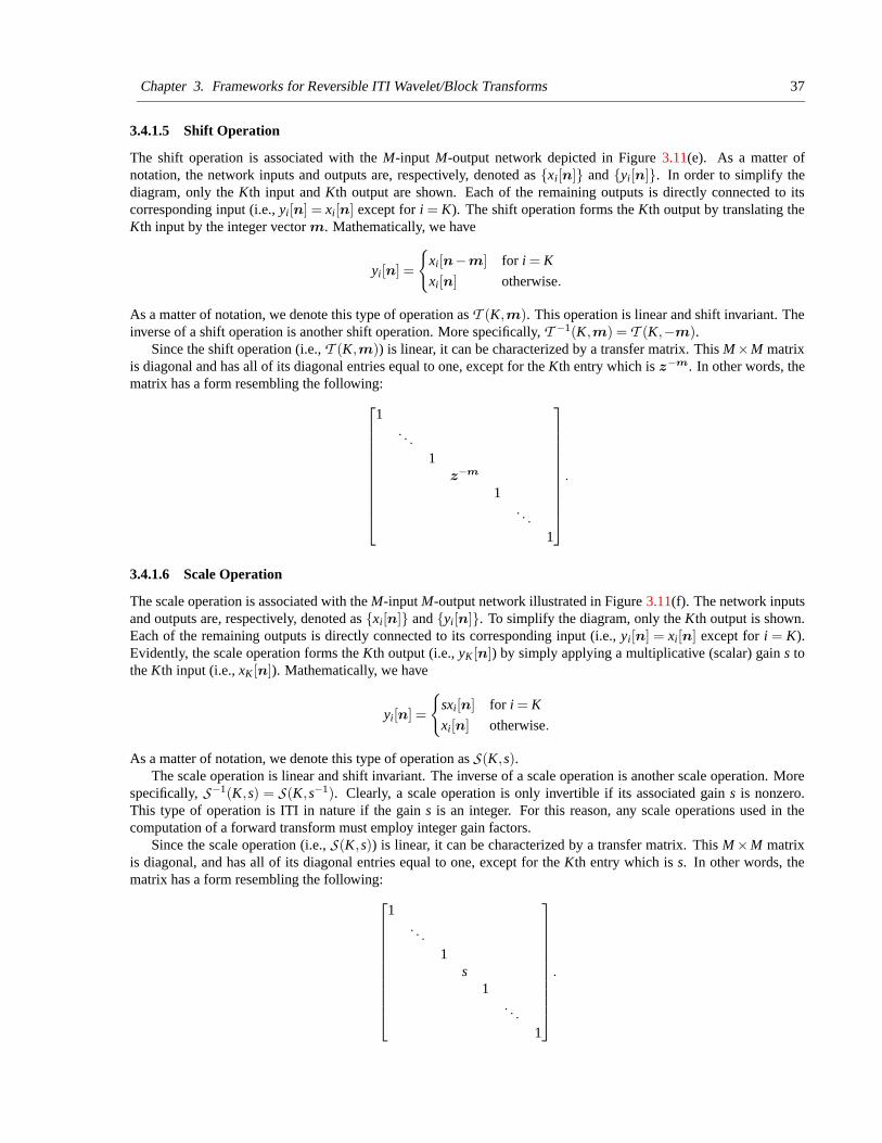
Chapter 3. Frameworks for Reversible ITI Wavelet/Block Transforms 37
3.4.1.5 Shift Operation
The shift operation is associated with the M-input M-output network depicted in Figure 3.11(e). As a matter ofnotation, the network inputs and outputs are, respectively, denoted as {xi[n]} and {yi[n]}. In order to simplify thediagram, only the Kth input and Kth output are shown. Each of the remaining outputs is directly connected to itscorresponding input (i.e., yi[n] = xi[n] except for i = K). The shift operation forms the Kth output by translating theKth input by the integer vector m. Mathematically, we have
yi[n] =
{
xi[n−m] for i = K
xi[n] otherwise.
As a matter of notation, we denote this type of operation as T (K,m). This operation is linear and shift invariant. Theinverse of a shift operation is another shift operation. More specifically, T −1(K,m) = T (K,−m).
Since the shift operation (i.e., T (K,m)) is linear, it can be characterized by a transfer matrix. This M×M matrixis diagonal and has all of its diagonal entries equal to one, except for the Kth entry which is z−m. In other words, thematrix has a form resembling the following:
1. . .
1z−m
1. . .
1
.
3.4.1.6 Scale Operation
The scale operation is associated with the M-input M-output network illustrated in Figure 3.11(f). The network inputsand outputs are, respectively, denoted as {xi[n]} and {yi[n]}. To simplify the diagram, only the Kth output is shown.Each of the remaining outputs is directly connected to its corresponding input (i.e., yi[n] = xi[n] except for i = K).Evidently, the scale operation forms the Kth output (i.e., yK [n]) by simply applying a multiplicative (scalar) gain s tothe Kth input (i.e., xK [n]). Mathematically, we have
yi[n] =
{
sxi[n] for i = K
xi[n] otherwise.
As a matter of notation, we denote this type of operation as S(K,s).The scale operation is linear and shift invariant. The inverse of a scale operation is another scale operation. More
specifically, S−1(K,s) = S(K,s−1). Clearly, a scale operation is only invertible if its associated gain s is nonzero.This type of operation is ITI in nature if the gain s is an integer. For this reason, any scale operations used in thecomputation of a forward transform must employ integer gain factors.
Since the scale operation (i.e., S(K,s)) is linear, it can be characterized by a transfer matrix. This M ×M matrixis diagonal, and has all of its diagonal entries equal to one, except for the Kth entry which is s. In other words, thematrix has a form resembling the following:
1. . .
1s
1. . .
1
.
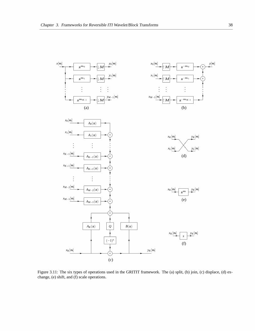
Chapter 3. Frameworks for Reversible ITI Wavelet/Block Transforms 38
-
-
-
-
-
-?
?
?
-
-
-
-
......
...
x[n]↓M
↓M
↓M
zm0
zmM−1
zm1
...
y0[n]
y1[n]
yM−1[n]
(a)
j+
j+
-
-
-
- -
- -
6
6
6
-
-
-
......
...
↑M
↑M
y[n]
z−mM−1
z−m1
z−m0
↑M
...xM−1[n]
x1[n]
x0[n]
(b)
A0(z)
A1(z) j+
AK+1(z) j+
AK−1(z) j+
AM−2(z)
AM−1(z)
j+
j+
j+
QAK(z) B(z)
j+
-
-
-
-
-
-
-
-
-
-
-
?
?
?
?
?
?
?
?
?
?66
6 6
----
-
......
...
xK+1[n]
xK−1[n]
x1[n]
x0[n]
...
xM−1[n]
xM−2[n]
......
(−1)s
xK [n] yK [n]
(c)
\\
\��
�-
-
-
-
xK [n]
xL[n]
yK [n]
yL[n]
(d)
- -yK [n]z
mxK [n]
(e)
-- yK [n]xK [n]s
(f)
Figure 3.11: The six types of operations used in the GRITIT framework. The (a) split, (b) join, (c) displace, (d) ex-change, (e) shift, and (f) scale operations.
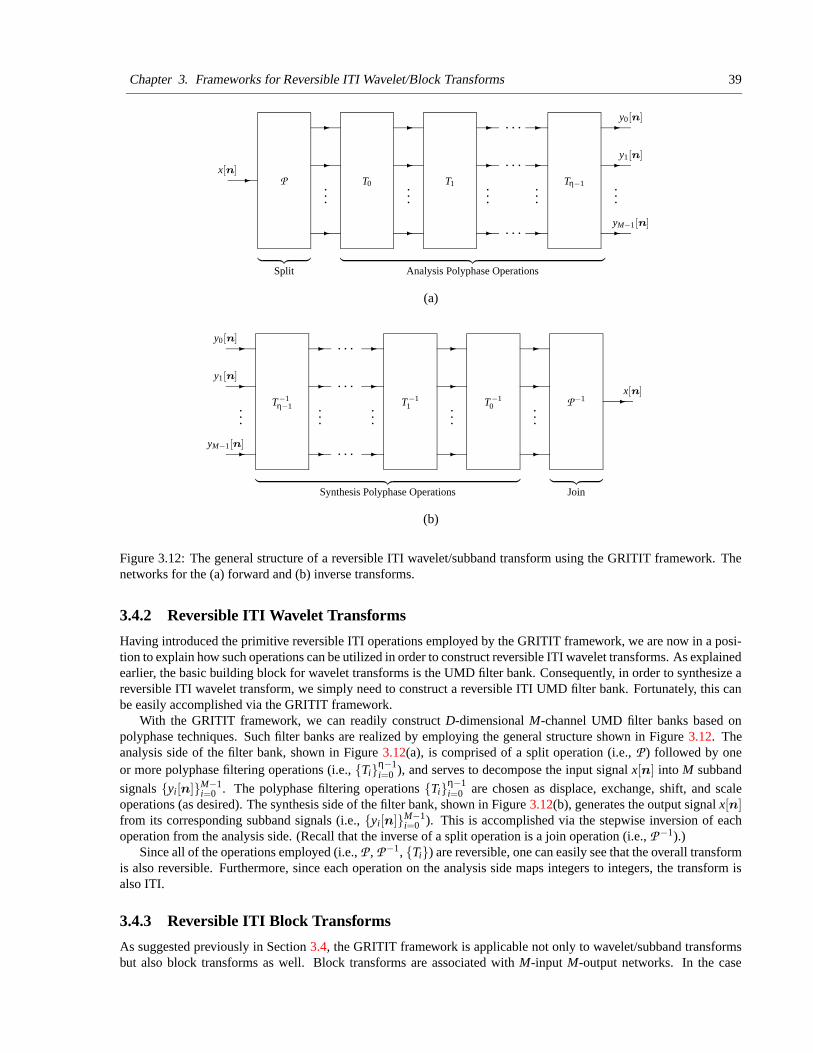
Chapter 3. Frameworks for Reversible ITI Wavelet/Block Transforms 39
︸ ︷︷ ︸
Analysis Polyphase Operations︸ ︷︷ ︸
Split
· · ·
· · ·
· · ·
-
-
-
-
- -
- -
-
-
......
x[n]
- y0[n]
y1[n]
yM−1[n]
...
-
-
-
-
-
......
P T0 T1 Tη−1
(a)
︸ ︷︷ ︸
Join︸ ︷︷ ︸
Synthesis Polyphase Operations
· · ·
· · ·
· · ·
-
--
-
--
--
-
-
......
x[n]
...
y0[n]
y1[n]
yM−1[n] -
-
--
......
-
-T−1
η−1 T−11 T−1
0 P−1
(b)
Figure 3.12: The general structure of a reversible ITI wavelet/subband transform using the GRITIT framework. Thenetworks for the (a) forward and (b) inverse transforms.
3.4.2 Reversible ITI Wavelet Transforms
Having introduced the primitive reversible ITI operations employed by the GRITIT framework, we are now in a posi-tion to explain how such operations can be utilized in order to construct reversible ITI wavelet transforms. As explainedearlier, the basic building block for wavelet transforms is the UMD filter bank. Consequently, in order to synthesize areversible ITI wavelet transform, we simply need to construct a reversible ITI UMD filter bank. Fortunately, this canbe easily accomplished via the GRITIT framework.
With the GRITIT framework, we can readily construct D-dimensional M-channel UMD filter banks based onpolyphase techniques. Such filter banks are realized by employing the general structure shown in Figure 3.12. Theanalysis side of the filter bank, shown in Figure 3.12(a), is comprised of a split operation (i.e., P ) followed by oneor more polyphase filtering operations (i.e., {Ti}η−1
i=0 ), and serves to decompose the input signal x[n] into M subband
signals {yi[n]}M−1i=0 . The polyphase filtering operations {Ti}η−1
i=0 are chosen as displace, exchange, shift, and scaleoperations (as desired). The synthesis side of the filter bank, shown in Figure 3.12(b), generates the output signal x[n]from its corresponding subband signals (i.e., {yi[n]}M−1
i=0 ). This is accomplished via the stepwise inversion of eachoperation from the analysis side. (Recall that the inverse of a split operation is a join operation (i.e., P −1).)
Since all of the operations employed (i.e., P , P−1, {Ti}) are reversible, one can easily see that the overall transformis also reversible. Furthermore, since each operation on the analysis side maps integers to integers, the transform isalso ITI.
3.4.3 Reversible ITI Block Transforms
As suggested previously in Section 3.4, the GRITIT framework is applicable not only to wavelet/subband transformsbut also block transforms as well. Block transforms are associated with M-input M-output networks. In the case
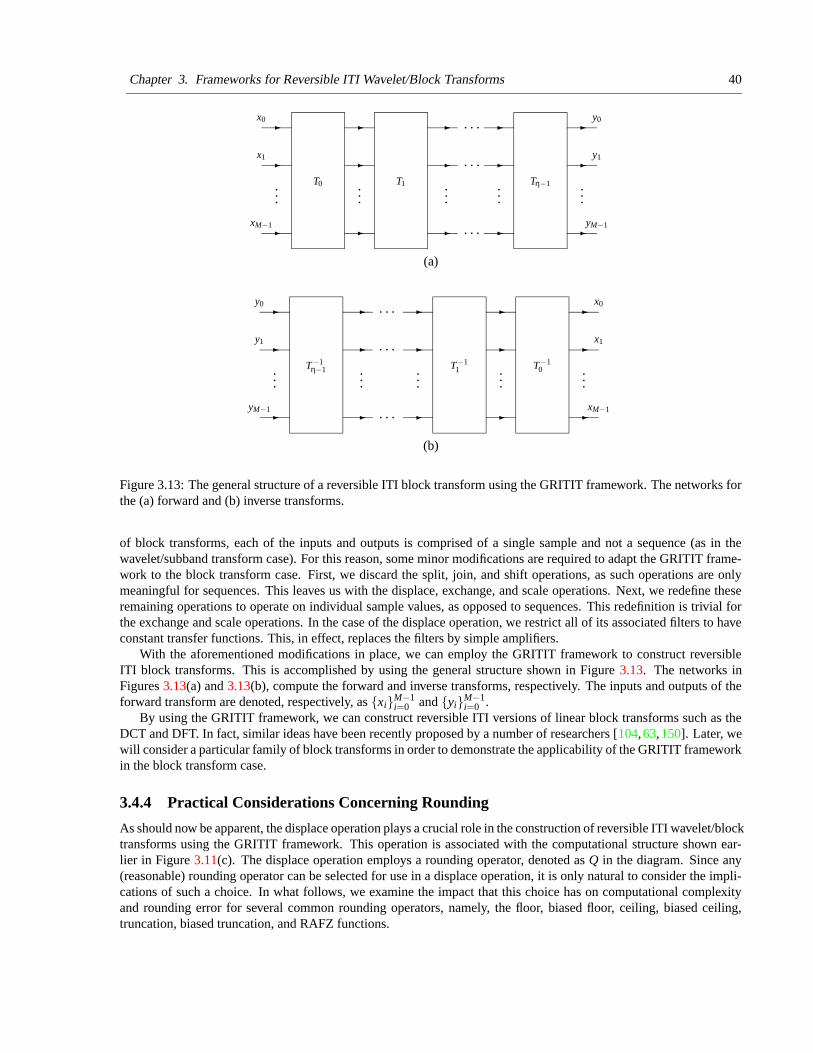
Chapter 3. Frameworks for Reversible ITI Wavelet/Block Transforms 40
· · ·
· · ·
· · ·- - --
-
-- -
-
-
-
-
-
-
y0
y1
......
yM−1-
T0 T1 Tη−1......
...
x0
x1
xM−1
(a)
· · ·
· · ·
· · ·
- -
- -
-
-
-
-
-
-
-
-
-
-
-
...T−1
η−1 ...T−1
1......
y0
y1
yM−1
...T−1
0
x0
x1
xM−1
(b)
Figure 3.13: The general structure of a reversible ITI block transform using the GRITIT framework. The networks forthe (a) forward and (b) inverse transforms.
of block transforms, each of the inputs and outputs is comprised of a single sample and not a sequence (as in thewavelet/subband transform case). For this reason, some minor modifications are required to adapt the GRITIT frame-work to the block transform case. First, we discard the split, join, and shift operations, as such operations are onlymeaningful for sequences. This leaves us with the displace, exchange, and scale operations. Next, we redefine theseremaining operations to operate on individual sample values, as opposed to sequences. This redefinition is trivial forthe exchange and scale operations. In the case of the displace operation, we restrict all of its associated filters to haveconstant transfer functions. This, in effect, replaces the filters by simple amplifiers.
With the aforementioned modifications in place, we can employ the GRITIT framework to construct reversibleITI block transforms. This is accomplished by using the general structure shown in Figure 3.13. The networks inFigures 3.13(a) and 3.13(b), compute the forward and inverse transforms, respectively. The inputs and outputs of theforward transform are denoted, respectively, as {xi}M−1
i=0 and {yi}M−1i=0 .
By using the GRITIT framework, we can construct reversible ITI versions of linear block transforms such as theDCT and DFT. In fact, similar ideas have been recently proposed by a number of researchers [104,63,150]. Later, wewill consider a particular family of block transforms in order to demonstrate the applicability of the GRITIT frameworkin the block transform case.
3.4.4 Practical Considerations Concerning Rounding
As should now be apparent, the displace operation plays a crucial role in the construction of reversible ITI wavelet/blocktransforms using the GRITIT framework. This operation is associated with the computational structure shown ear-lier in Figure 3.11(c). The displace operation employs a rounding operator, denoted as Q in the diagram. Since any(reasonable) rounding operator can be selected for use in a displace operation, it is only natural to consider the impli-cations of such a choice. In what follows, we examine the impact that this choice has on computational complexityand rounding error for several common rounding operators, namely, the floor, biased floor, ceiling, biased ceiling,truncation, biased truncation, and RAFZ functions.
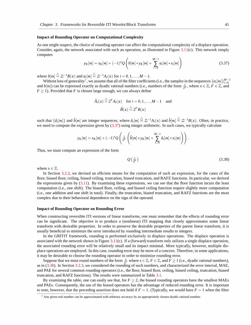
Chapter 3. Frameworks for Reversible ITI Wavelet/Block Transforms 41
Impact of Rounding Operator on Computational Complexity
As one might suspect, the choice of rounding operator can affect the computational complexity of a displace operation.Consider, again, the network associated with such an operation, as illustrated in Figure 3.11(c). This network simplycomputes
yK [n] = xK [n]+ (−1)sQ
(
b[n]∗ yK [n]+M−1
∑i=0
ai[n]∗ xi[n]
)
(3.37)
where b[n]4= Z−1B(z) and ai[n]
4= Z−1Ai(z) for i = 0,1, . . . ,M−1.
Without loss of generality1, we assume that all of the filter coefficients (i.e., the samples in the sequences {ai[n]}M−1i=0
and b[n]) can be expressed exactly as dyadic rational numbers (i.e., numbers of the form x2F , where x ∈ Z, F ∈ Z, and
F ≥ 1). Provided that F is chosen large enough, we can always define
Ai(z)4= 2F Ai(z) for i = 0,1, . . . ,M−1 and
B(z)4= 2F B(z)
such that {ai[n]} and b[n] are integer sequences, where ai[n]4= Z−1Ai(z) and b[n]
4= Z−1B(z). Often, in practice,
we need to compute the expression given by (3.37) using integer arithmetic. In such cases, we typically calculate
yK [n] = xK [n]+ (−1)sQ
(
12F
(
b[n]∗ yK [n]+M−1
∑i=0
ai[n]∗ xi[n]
))
.
Thus, we must compute an expression of the form
Q(
x2F
)(3.38)
where x ∈ Z.In Section 3.2.2, we devised an efficient means for the computation of such an expression, for the cases of the
floor, biased floor, ceiling, biased ceiling, truncation, biased truncation, and RAFZ functions. In particular, we derivedthe expressions given by (3.11). By examining these expressions, we can see that the floor function incurs the leastcomputation (i.e., one shift). The biased floor, ceiling, and biased ceiling function require slightly more computation(i.e., one addition and one shift in total). Finally, the truncation, biased truncation, and RAFZ functions are the mostcomplex due to their behavioral dependence on the sign of the operand.
Impact of Rounding Operator on Rounding Error
When constructing reversible ITI versions of linear transforms, one must remember that the effects of rounding errorcan be significant. The objective is to produce a (nonlinear) ITI mapping that closely approximates some lineartransform with desirable properties. In order to preserve the desirable properties of the parent linear transform, it isusually beneficial to minimize the error introduced by rounding intermediate results to integers.
In the GRITIT framework, rounding is performed exclusively in displace operations. The displace operation isassociated with the network shown in Figure 3.11(c). If a (forward) transform only utilizes a single displace operation,the associated rounding error will be relatively small and its impact minimal. More typically, however, multiple dis-place operations are employed. In this case, rounding error may be more of a concern. Therefore, in some applications,it may be desirable to choose the rounding operator in order to minimize rounding error.
Suppose that we must round numbers of the form x2F where x ∈Z, F ∈Z, and F ≥ 1 (i.e., dyadic rational numbers),
as in (3.38). In Section 3.2.3, we considered the rounding of such numbers, and characterized the error interval, MAE,and PAE for several common rounding operators (i.e., the floor, biased floor, ceiling, biased ceiling, truncation, biasedtruncation, and RAFZ functions). The results were summarized in Table 3.1.
By examining the table, one can easily see that, for F ≥ 2, the biased rounding operators have the smallest MAEsand PAEs. Consequently, the use of the biased operators has the advantage of reduced rounding error. It is importantto note, however, that the preceding assertion does not hold if F = 1. (Typically, we would have F = 1 when the filter
1 Any given real number can be approximated with arbitrary accuracy by an appropriately chosen dyadic rational number.
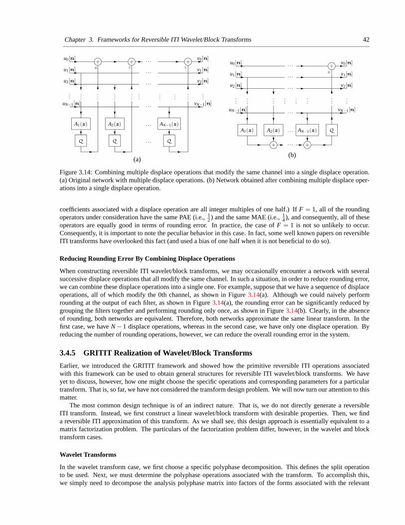
Chapter 3. Frameworks for Reversible ITI Wavelet/Block Transforms 42
Q Q
j+j+ j+
Q
-
-
-
-
?
?
? ?
?
6?6
- -
- -
-
-
-
-
-
6
?
?
-
u0[n]
u1[n]
u2[n]
A1(z)
......
uN−1[n]
A2(z)
......
......
. . .
. . .
. . .
. . .
. . .
. . .
± ±
v0[n]
v1[n]
v2[n]
......
......
±
AN−1(z)
vN−1[n]
(a)
j+
j+
Q
j+
-
-
-
?-
?
-
?
?-
?
-
6
6
-
-
-
-?
?
-
-
-
-
-
u0[n]
u1[n]
u2[n]
A1(z)
uN−1[n]
......
A2(z)
...
. . .
. . .
. . .
. . .
. . .
. . .
±
...
v0[n]
vN−1[n]
v2[n]
v1[n]
...
AN−1(z)
......
...
(b)
Figure 3.14: Combining multiple displace operations that modify the same channel into a single displace operation.(a) Original network with multiple displace operations. (b) Network obtained after combining multiple displace oper-ations into a single displace operation.
coefficients associated with a displace operation are all integer multiples of one half.) If F = 1, all of the roundingoperators under consideration have the same PAE (i.e., 1
2 ) and the same MAE (i.e., 14 ), and consequently, all of these
operators are equally good in terms of rounding error. In practice, the case of F = 1 is not so unlikely to occur.Consequently, it is important to note the peculiar behavior in this case. In fact, some well known papers on reversibleITI transforms have overlooked this fact (and used a bias of one half when it is not beneficial to do so).
Reducing Rounding Error By Combining Displace Operations
When constructing reversible ITI wavelet/block transforms, we may occasionally encounter a network with severalsuccessive displace operations that all modify the same channel. In such a situation, in order to reduce rounding error,we can combine these displace operations into a single one. For example, suppose that we have a sequence of displaceoperations, all of which modify the 0th channel, as shown in Figure 3.14(a). Although we could naively performrounding at the output of each filter, as shown in Figure 3.14(a), the rounding error can be significantly reduced bygrouping the filters together and performing rounding only once, as shown in Figure 3.14(b). Clearly, in the absenceof rounding, both networks are equivalent. Therefore, both networks approximate the same linear transform. In thefirst case, we have N − 1 displace operations, whereas in the second case, we have only one displace operation. Byreducing the number of rounding operations, however, we can reduce the overall rounding error in the system.
3.4.5 GRITIT Realization of Wavelet/Block Transforms
Earlier, we introduced the GRITIT framework and showed how the primitive reversible ITI operations associatedwith this framework can be used to obtain general structures for reversible ITI wavelet/block transforms. We haveyet to discuss, however, how one might choose the specific operations and corresponding parameters for a particulartransform. That is, so far, we have not considered the transform design problem. We will now turn our attention to thismatter.
The most common design technique is of an indirect nature. That is, we do not directly generate a reversibleITI transform. Instead, we first construct a linear wavelet/block transform with desirable properties. Then, we finda reversible ITI approximation of this transform. As we shall see, this design approach is essentially equivalent to amatrix factorization problem. The particulars of the factorization problem differ, however, in the wavelet and blocktransform cases.
Wavelet Transforms
In the wavelet transform case, we first choose a specific polyphase decomposition. This defines the split operationto be used. Next, we must determine the polyphase operations associated with the transform. To accomplish this,we simply need to decompose the analysis polyphase matrix into factors of the forms associated with the relevant
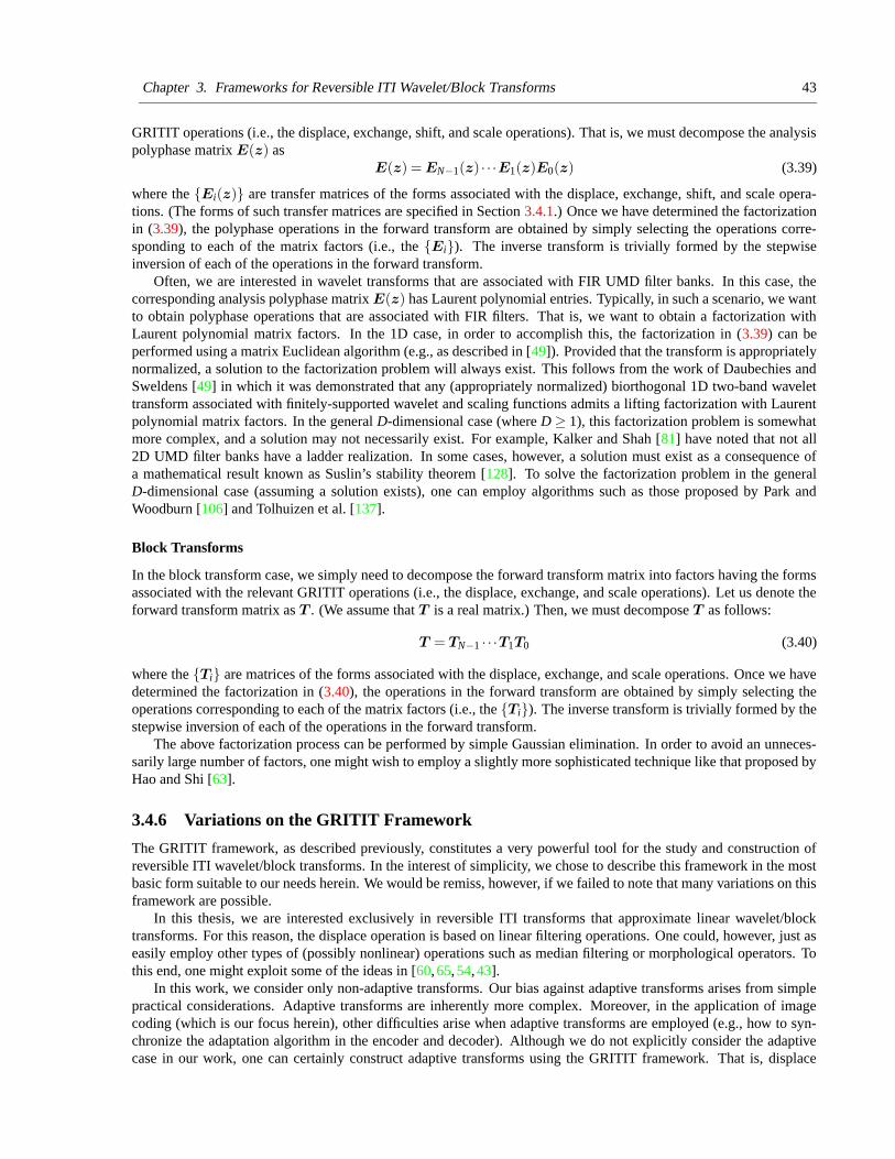
Chapter 3. Frameworks for Reversible ITI Wavelet/Block Transforms 43
GRITIT operations (i.e., the displace, exchange, shift, and scale operations). That is, we must decompose the analysispolyphase matrix E(z) as
E(z) = EN−1(z) · · ·E1(z)E0(z) (3.39)
where the {Ei(z)} are transfer matrices of the forms associated with the displace, exchange, shift, and scale opera-tions. (The forms of such transfer matrices are specified in Section 3.4.1.) Once we have determined the factorizationin (3.39), the polyphase operations in the forward transform are obtained by simply selecting the operations corre-sponding to each of the matrix factors (i.e., the {Ei}). The inverse transform is trivially formed by the stepwiseinversion of each of the operations in the forward transform.
Often, we are interested in wavelet transforms that are associated with FIR UMD filter banks. In this case, thecorresponding analysis polyphase matrix E(z) has Laurent polynomial entries. Typically, in such a scenario, we wantto obtain polyphase operations that are associated with FIR filters. That is, we want to obtain a factorization withLaurent polynomial matrix factors. In the 1D case, in order to accomplish this, the factorization in (3.39) can beperformed using a matrix Euclidean algorithm (e.g., as described in [49]). Provided that the transform is appropriatelynormalized, a solution to the factorization problem will always exist. This follows from the work of Daubechies andSweldens [49] in which it was demonstrated that any (appropriately normalized) biorthogonal 1D two-band wavelettransform associated with finitely-supported wavelet and scaling functions admits a lifting factorization with Laurentpolynomial matrix factors. In the general D-dimensional case (where D ≥ 1), this factorization problem is somewhatmore complex, and a solution may not necessarily exist. For example, Kalker and Shah [81] have noted that not all2D UMD filter banks have a ladder realization. In some cases, however, a solution must exist as a consequence ofa mathematical result known as Suslin’s stability theorem [128]. To solve the factorization problem in the generalD-dimensional case (assuming a solution exists), one can employ algorithms such as those proposed by Park andWoodburn [106] and Tolhuizen et al. [137].
Block Transforms
In the block transform case, we simply need to decompose the forward transform matrix into factors having the formsassociated with the relevant GRITIT operations (i.e., the displace, exchange, and scale operations). Let us denote theforward transform matrix as T . (We assume that T is a real matrix.) Then, we must decompose T as follows:
T = TN−1 · · ·T1T0 (3.40)
where the {Ti} are matrices of the forms associated with the displace, exchange, and scale operations. Once we havedetermined the factorization in (3.40), the operations in the forward transform are obtained by simply selecting theoperations corresponding to each of the matrix factors (i.e., the {Ti}). The inverse transform is trivially formed by thestepwise inversion of each of the operations in the forward transform.
The above factorization process can be performed by simple Gaussian elimination. In order to avoid an unneces-sarily large number of factors, one might wish to employ a slightly more sophisticated technique like that proposed byHao and Shi [63].
3.4.6 Variations on the GRITIT Framework
The GRITIT framework, as described previously, constitutes a very powerful tool for the study and construction ofreversible ITI wavelet/block transforms. In the interest of simplicity, we chose to describe this framework in the mostbasic form suitable to our needs herein. We would be remiss, however, if we failed to note that many variations on thisframework are possible.
In this thesis, we are interested exclusively in reversible ITI transforms that approximate linear wavelet/blocktransforms. For this reason, the displace operation is based on linear filtering operations. One could, however, just aseasily employ other types of (possibly nonlinear) operations such as median filtering or morphological operators. Tothis end, one might exploit some of the ideas in [60, 65, 54, 43].
In this work, we consider only non-adaptive transforms. Our bias against adaptive transforms arises from simplepractical considerations. Adaptive transforms are inherently more complex. Moreover, in the application of imagecoding (which is our focus herein), other difficulties arise when adaptive transforms are employed (e.g., how to syn-chronize the adaptation algorithm in the encoder and decoder). Although we do not explicitly consider the adaptivecase in our work, one can certainly construct adaptive transforms using the GRITIT framework. That is, displace
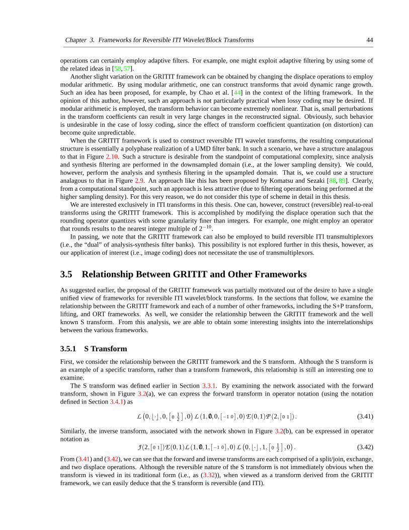
Chapter 3. Frameworks for Reversible ITI Wavelet/Block Transforms 44
operations can certainly employ adaptive filters. For example, one might exploit adaptive filtering by using some ofthe related ideas in [58, 57].
Another slight variation on the GRITIT framework can be obtained by changing the displace operations to employmodular arithmetic. By using modular arithmetic, one can construct transforms that avoid dynamic range growth.Such an idea has been proposed, for example, by Chao et al. [44] in the context of the lifting framework. In theopinion of this author, however, such an approach is not particularly practical when lossy coding may be desired. Ifmodular arithmetic is employed, the transform behavior can become extremely nonlinear. That is, small perturbationsin the transform coefficients can result in very large changes in the reconstructed signal. Obviously, such behavioris undesirable in the case of lossy coding, since the effect of transform coefficient quantization (on distortion) canbecome quite unpredictable.
When the GRITIT framework is used to construct reversible ITI wavelet transforms, the resulting computationalstructure is essentially a polyphase realization of a UMD filter bank. In such a scenario, we have a structure analagousto that in Figure 2.10. Such a structure is desirable from the standpoint of computational complexity, since analysisand synthesis filtering are performed in the downsampled domain (i.e., at the lower sampling density). We could,however, perform the analysis and synthesis filtering in the upsampled domain. That is, we could use a structureanalagous to that in Figure 2.9. An approach like this has been proposed by Komatsu and Sezaki [88, 89]. Clearly,from a computational standpoint, such an approach is less attractive (due to filtering operations being performed at thehigher sampling density). For this very reason, we do not consider this type of scheme in detail in this thesis.
We are interested exclusively in ITI transforms in this thesis. One can, however, construct (reversible) real-to-realtransforms using the GRITIT framework. This is accomplished by modifying the displace operation such that therounding operator quantizes with some granularity finer than integers. For example, one might employ an operatorthat rounds results to the nearest integer multiple of 2−10.
In passing, we note that the GRITIT framework can also be employed to build reversible ITI transmultiplexors(i.e., the “dual” of analysis-synthesis filter banks). This possibility is not explored further in this thesis, however, asour application of interest (i.e., image coding) does not necessitate the use of transmultiplexors.
3.5 Relationship Between GRITIT and Other Frameworks
As suggested earlier, the proposal of the GRITIT framework was partially motivated out of the desire to have a singleunified view of frameworks for reversible ITI wavelet/block transforms. In the sections that follow, we examine therelationship between the GRITIT framework and each of a number of other frameworks, including the S+P transform,lifting, and ORT frameworks. As well, we consider the relationship between the GRITIT framework and the wellknown S transform. From this analysis, we are able to obtain some interesting insights into the interrelationshipsbetween the various frameworks.
3.5.1 S Transform
First, we consider the relationship between the GRITIT framework and the S transform. Although the S transform isan example of a specific transform, rather than a transform framework, this relationship is still an interesting one toexamine.
The S transform was defined earlier in Section 3.3.1. By examining the network associated with the forwardtransform, shown in Figure 3.2(a), we can express the forward transform in operator notation (using the notationdefined in Section 3.4.1) as
L(0,b·c ,0,
[0 1
2
],0)
L (1, /0,0, [−1 0 ] ,0)E(0,1)P (2, [ 0 1 ]) . (3.41)
Similarly, the inverse transform, associated with the network shown in Figure 3.2(b), can be expressed in operatornotation as
J (2, [ 0 1 ])E(0,1)L (1, /0,1, [−1 0 ] ,0)L(0,b·c ,1,
[0 1
2
],0). (3.42)
From (3.41) and (3.42), we can see that the forward and inverse transforms are each comprised of a split/join, exchange,and two displace operations. Although the reversible nature of the S transform is not immediately obvious when thetransform is viewed in its traditional form (i.e., as (3.32)), when viewed as a transform derived from the GRITITframework, we can easily deduce that the S transform is reversible (and ITI).
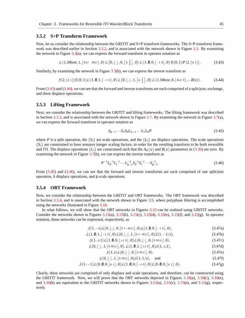
Chapter 3. Frameworks for Reversible ITI Wavelet/Block Transforms 45
3.5.2 S+P Transform Framework
Now, let us consider the relationship between the GRITIT and S+P transform frameworks. The S+P transform frame-work was described earlier in Section 3.3.2, and is associated with the network shown in Figure 3.3. By examiningthe network in Figure 3.3(a), we can express the forward transform in operator notation as
L (1,bfloor,1, [A(z) −B(z) ] ,0)L(0,b·c ,0,
[0 1
2
],0)
L (1, /0,0, [−1 0 ] ,0)E(0,1)P (2, [ 0 1 ]) . (3.43)
Similarly, by examining the network in Figure 3.3(b), we can express the inverse transform as
J (2, [ 0 1 ])E(0,1)L (1, /0,1, [−1 0 ] ,0)L(0,b·c ,1,
[0 1
2
],0)
L (1,bfloor,0, [A(z) 0 ] ,−B(z)) . (3.44)
From (3.43) and (3.44), we can see that the forward and inverse transforms are each comprised of a split/join, exchange,and three displace operations.
3.5.3 Lifting Framework
Next, we consider the relationship between the GRITIT and lifting frameworks. The lifting framework was describedin Section 3.3.3, and is associated with the network shown in Figure 3.7. By examining the network in Figure 3.7(a),we can express the forward transform in operator notation as
Sρ−1 · · ·S1S0Lλ−1 · · ·L1L0P (3.45)
where P is a split operation, the {Si} are scale operations, and the {Li} are displace operations. The scale operations{Si} are constrained to have nonzero integer scaling factors, in order for the resulting transform to be both reversibleand ITI. The displace operations {Li} are constrained such that the AK(z) and B(z) parameters in (3.36) are zero. Byexamining the network in Figure 3.7(b), we can express the inverse transform as
P−1L−10 L−1
1 · · ·L−1λ−1S−1
0 S−11 · · ·S−1
ρ−1. (3.46)
From (3.45) and (3.46), we can see that the forward and inverse transforms are each comprised of one split/joinoperation, λ displace operations, and ρ scale operations.
3.5.4 ORT Framework
Now, we consider the relationship between the GRITIT and ORT frameworks. The ORT framework was describedin Section 3.3.4, and is associated with the network shown in Figure 3.9, where polyphase filtering is accomplishedusing the networks illustrated in Figure 3.10.
In what follows, we will show that the ORT networks in Figures 3.10 can be realized using GRITIT networks.Consider the networks shown in Figures 3.15(a), 3.15(b), 3.15(c), 3.15(d), 3.15(e), 3.15(f), and 3.15(g). In operatornotation, these networks can be expressed, respectively, as
S(1,−s)L(0,b·c ,0, [ 0 1−H(z) ] ,0)L(1, /0,0, [−1 0 ] ,0), (3.47a)
L(1, /0,1, [−1 0 ] ,0)L(0,b·c ,1, [ 0 1−H(z) ] ,0)S(1,−1/s), (3.47b)
S(1,±1)L(1, /0,0, [±1 0 ] ,0)L(0,b·c ,0, [ 0 H(z) ] ,0), (3.47c)
L(0,b·c ,1, [ 0 H(z) ] ,0),L(1, /0,1, [±1 0 ] ,0)S(1,±1), (3.47d)
S(1,s)L(0,b·c ,0, [ 0 H(z) ] ,0), (3.47e)
L(0,b·c ,1, [ 0 H(z) ] ,0)S(1,1/s), and (3.47f)
S(1,−1)L(0, /0,0, [0 1 ] ,0)L(1, /0,0, [−1 0 ] ,0)L(0, /0,0, [ 0 1 ] ,0). (3.47g)
Clearly, these networks are comprised of only displace and scale operations, and therefore, can be constructed usingthe GRITIT framework. Now, we will prove that the ORT networks depicted in Figures 3.10(a), 3.10(c), 3.10(e),and 3.10(h) are equivalent to the GRITIT networks shown in Figures 3.15(a), 3.15(c), 3.15(e), and 3.15(g), respec-tively.
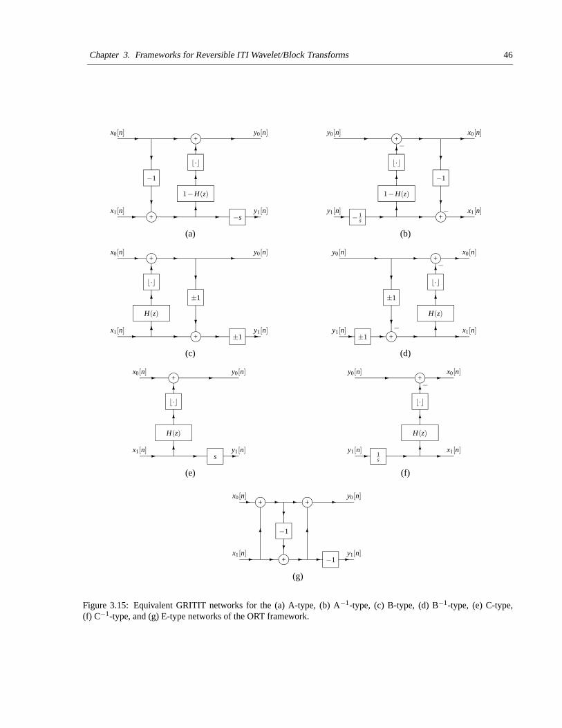
Chapter 3. Frameworks for Reversible ITI Wavelet/Block Transforms 46
j+
b·c
j+
−1
−s
6
- -
---
-
6
6 -?
?
y1[n]
y0[n]x0[n]
x1[n]
1−H(z)
(a)
b·c
j+
j+
− 1s
1−H(z)
−1
- -
-
6
6
6 ?
?-
--
-y1[n]
x0[n]y0[n]
x1[n]
−
−
(b)
b·c
j+
j+
±1
±1- -
--
- -
6
6
6 ?
?
-
y1[n]
y0[n]x0[n]
x1[n]
H(z)
(c)
j+
b·c
j+
H(z)
±1
±1
6
- -
--
6
6?
?
-
-
- x1[n]y1[n]
x0[n]y0[n]
−
−
(d)
j+
b·c
s
H(z)
6
- -
--
6
6 -y1[n]
y0[n]
x1[n]
x0[n]
(e)
j+
b·c
H(z)
1s
6
6
- -
6- --
y0[n] x0[n]
x1[n]y1[n]
−
(f)
j+
j+
j+
−1
−1
- - - - -
6 6
?
?
- - - -
y1[n]
x0[n]
x1[n]
y0[n]
(g)
Figure 3.15: Equivalent GRITIT networks for the (a) A-type, (b) A−1-type, (c) B-type, (d) B−1-type, (e) C-type,(f) C−1-type, and (g) E-type networks of the ORT framework.
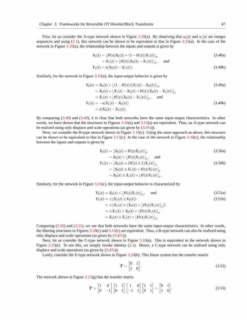
Chapter 3. Frameworks for Reversible ITI Wavelet/Block Transforms 47
First, let us consider the A-type network shown in Figure 3.10(a). By observing that x0[n] and x1[n] are integersequences and using (2.1), this network can be shown to be equivalent to that in Figure 3.15(a). In the case of thenetwork in Figure 3.10(a), the relationship between the inputs and outputs is given by
Y0(z) = bH(z)X0(z)+(1−H(z))X1(z)cz (3.48a)
= X1(z)+ bH(z)(X0(z)−X1(z))cz , and
Y1(z) = s(X0(z)−X1(z)). (3.48b)
Similarly, for the network in Figure 3.15(a), the input-output behavior is given by
Y0(z) = X0(z)+ b(1−H(z))(X1(z)−X0(z))cz (3.49a)
= X0(z)+ bX1(z)−X0(z)+H(z)(X0(z)−X1(z))cz
= X1(z)+ bH(z)(X0(z)−X1(z))cz , and
Y1(z) = −s(X1(z)−X0(z)) (3.49b)
= s(X0(z)−X1(z)).
By comparing (3.48) and (3.49), it is clear that both networks have the same input-output characteristics. In otherwords, we have shown that the structures in Figures 3.10(a) and 3.15(a) are equivalent. Thus, an A-type network canbe realized using only displace and scale operations (as given by (3.47a)).
Next, we consider the B-type network shown in Figure 3.10(c). Using the same approach as above, this structurecan be shown to be equivalent to that in Figure 3.15(c). In the case of the network in Figure 3.10(c), the relationshipbetween the inputs and outputs is given by
Y0(z) = bX0(z)+H(z)X1(z)cz (3.50a)
= X0(z)+ bH(z)X1(z)cz , and
Y1(z) = bX0(z)+(H(z)±1)X1(z)cz (3.50b)
= bX0(z)±X1(z)+H(z)X1(z)cz
= X0(z)±X1(z)+ bH(z)X1(z)cz .
Similarly, for the network in Figure 3.15(c), the input-output behavior is characterized by
Y0(z) = X0(z)+ bH(z)X1(z)cz , and (3.51a)
Y1(z) = ±(X1(z)±Y0(z)) (3.51b)
= ±(X1(z)± (X0(z)+ bH(z)X1(z)cz))
= ±X1(z)+X0(z)+ bH(z)X1(z)cz
= X0(z)±X1(z)+ bH(z)X1(z)cz .
Comparing (3.50) and (3.51), we see that both networks have the same input-output characteristics. In other words,the filtering structures in Figures 3.10(c) and 3.15(c) are equivalent. Thus, a B-type network can also be realized usingonly displace and scale operations (as given by (3.47c)).
Next, let us consider the C-type network shown in Figure 3.10(e). This is equivalent to the network shown inFigure 3.15(e). To see this, we simply invoke identity (2.1). Hence, a C-type network can be realized using onlydisplace and scale operations (as given by (3.47e)).
Lastly, consider the E-type network shown in Figure 3.10(h). This linear system has the transfer matrix
T =
[0 11 0
]
. (3.52)
The network shown in Figure 3.15(g) has the transfer matrix
T =
[1 00 −1
][1 10 1
][1 0−1 1
][1 10 1
]
=
[0 11 0
]
. (3.53)
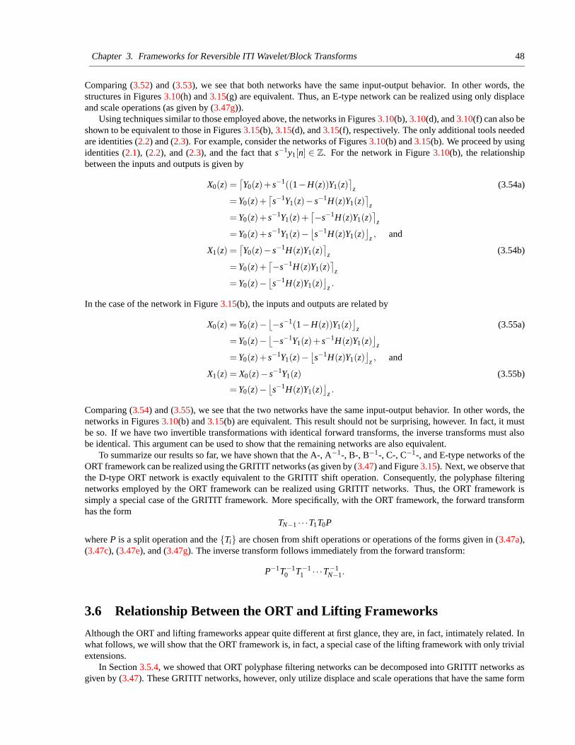
Chapter 3. Frameworks for Reversible ITI Wavelet/Block Transforms 48
Comparing (3.52) and (3.53), we see that both networks have the same input-output behavior. In other words, thestructures in Figures 3.10(h) and 3.15(g) are equivalent. Thus, an E-type network can be realized using only displaceand scale operations (as given by (3.47g)).
Using techniques similar to those employed above, the networks in Figures 3.10(b), 3.10(d), and 3.10(f) can also beshown to be equivalent to those in Figures 3.15(b), 3.15(d), and 3.15(f), respectively. The only additional tools neededare identities (2.2) and (2.3). For example, consider the networks of Figures 3.10(b) and 3.15(b). We proceed by usingidentities (2.1), (2.2), and (2.3), and the fact that s−1y1[n] ∈ Z. For the network in Figure 3.10(b), the relationshipbetween the inputs and outputs is given by
X0(z) =⌈Y0(z)+ s−1((1−H(z))Y1(z)
⌉
z (3.54a)
= Y0(z)+⌈s−1Y1(z)− s−1H(z)Y1(z)
⌉
z
= Y0(z)+ s−1Y1(z)+⌈−s−1H(z)Y1(z)
⌉
z
= Y0(z)+ s−1Y1(z)−⌊s−1H(z)Y1(z)
⌋
z , and
X1(z) =⌈Y0(z)− s−1H(z)Y1(z)
⌉
z (3.54b)
= Y0(z)+⌈−s−1H(z)Y1(z)
⌉
z
= Y0(z)−⌊s−1H(z)Y1(z)
⌋
z .
In the case of the network in Figure 3.15(b), the inputs and outputs are related by
X0(z) = Y0(z)−⌊−s−1(1−H(z))Y1(z)
⌋
z (3.55a)
= Y0(z)−⌊−s−1Y1(z)+ s−1H(z)Y1(z)
⌋
z
= Y0(z)+ s−1Y1(z)−⌊s−1H(z)Y1(z)
⌋
z , and
X1(z) = X0(z)− s−1Y1(z) (3.55b)
= Y0(z)−⌊s−1H(z)Y1(z)
⌋
z .
Comparing (3.54) and (3.55), we see that the two networks have the same input-output behavior. In other words, thenetworks in Figures 3.10(b) and 3.15(b) are equivalent. This result should not be surprising, however. In fact, it mustbe so. If we have two invertible transformations with identical forward transforms, the inverse transforms must alsobe identical. This argument can be used to show that the remaining networks are also equivalent.
To summarize our results so far, we have shown that the A-, A−1-, B-, B−1-, C-, C−1-, and E-type networks of theORT framework can be realized using the GRITIT networks (as given by (3.47) and Figure 3.15). Next, we observe thatthe D-type ORT network is exactly equivalent to the GRITIT shift operation. Consequently, the polyphase filteringnetworks employed by the ORT framework can be realized using GRITIT networks. Thus, the ORT framework issimply a special case of the GRITIT framework. More specifically, with the ORT framework, the forward transformhas the form
TN−1 · · ·T1T0P
where P is a split operation and the {Ti} are chosen from shift operations or operations of the forms given in (3.47a),(3.47c), (3.47e), and (3.47g). The inverse transform follows immediately from the forward transform:
P−1T−10 T−1
1 · · ·T−1N−1.
3.6 Relationship Between the ORT and Lifting Frameworks
Although the ORT and lifting frameworks appear quite different at first glance, they are, in fact, intimately related. Inwhat follows, we will show that the ORT framework is, in fact, a special case of the lifting framework with only trivialextensions.
In Section 3.5.4, we showed that ORT polyphase filtering networks can be decomposed into GRITIT networks asgiven by (3.47). These GRITIT networks, however, only utilize displace and scale operations that have the same form
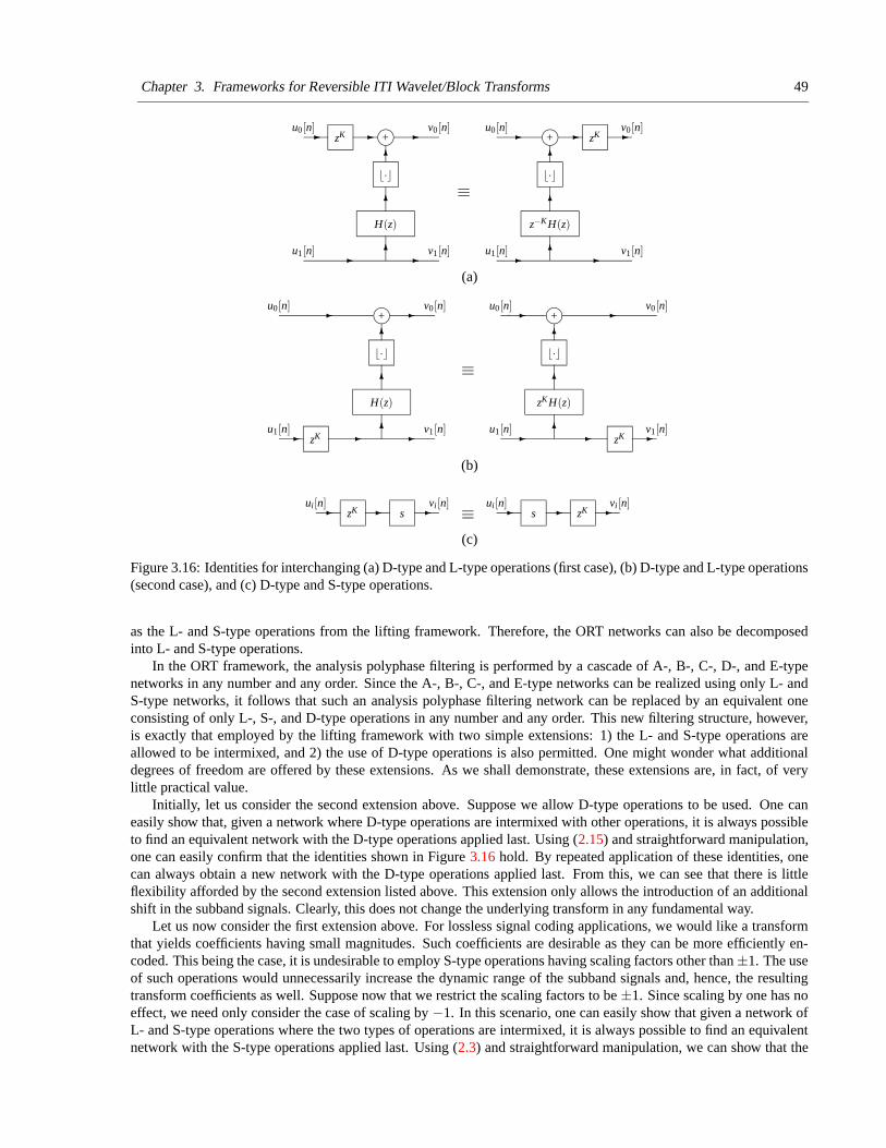
Chapter 3. Frameworks for Reversible ITI Wavelet/Block Transforms 49
j+
b·c
H(z)
zK j+
b·c
z−KH(z)
zK
6
6
-
6 -
--
-
6
-
-
6
6
- -
-
v0[n]
v1[n]u1[n]
u0[n]
≡
u1[n]
u0[n] v0[n]
v1[n]
(a)
j+
b·c
zK
H(z)
j+
b·c
zKH(z)
zK
6
6
- -
6- --
.
6
- -
--
6
6 -
u0[n] v0[n]
v1[n]u1[n]
≡
v1[n]
v0[n]
u1[n]
u0[n]
(b)
-- - -- -ui[n]zK
vi[n] ui[n]s
vi[n]≡ zKs
(c)
Figure 3.16: Identities for interchanging (a) D-type and L-type operations (first case), (b) D-type and L-type operations(second case), and (c) D-type and S-type operations.
as the L- and S-type operations from the lifting framework. Therefore, the ORT networks can also be decomposedinto L- and S-type operations.
In the ORT framework, the analysis polyphase filtering is performed by a cascade of A-, B-, C-, D-, and E-typenetworks in any number and any order. Since the A-, B-, C-, and E-type networks can be realized using only L- andS-type networks, it follows that such an analysis polyphase filtering network can be replaced by an equivalent oneconsisting of only L-, S-, and D-type operations in any number and any order. This new filtering structure, however,is exactly that employed by the lifting framework with two simple extensions: 1) the L- and S-type operations areallowed to be intermixed, and 2) the use of D-type operations is also permitted. One might wonder what additionaldegrees of freedom are offered by these extensions. As we shall demonstrate, these extensions are, in fact, of verylittle practical value.
Initially, let us consider the second extension above. Suppose we allow D-type operations to be used. One caneasily show that, given a network where D-type operations are intermixed with other operations, it is always possibleto find an equivalent network with the D-type operations applied last. Using (2.15) and straightforward manipulation,one can easily confirm that the identities shown in Figure 3.16 hold. By repeated application of these identities, onecan always obtain a new network with the D-type operations applied last. From this, we can see that there is littleflexibility afforded by the second extension listed above. This extension only allows the introduction of an additionalshift in the subband signals. Clearly, this does not change the underlying transform in any fundamental way.
Let us now consider the first extension above. For lossless signal coding applications, we would like a transformthat yields coefficients having small magnitudes. Such coefficients are desirable as they can be more efficiently en-coded. This being the case, it is undesirable to employ S-type operations having scaling factors other than ±1. The useof such operations would unnecessarily increase the dynamic range of the subband signals and, hence, the resultingtransform coefficients as well. Suppose now that we restrict the scaling factors to be ±1. Since scaling by one has noeffect, we need only consider the case of scaling by −1. In this scenario, one can easily show that given a network ofL- and S-type operations where the two types of operations are intermixed, it is always possible to find an equivalentnetwork with the S-type operations applied last. Using (2.3) and straightforward manipulation, we can show that the
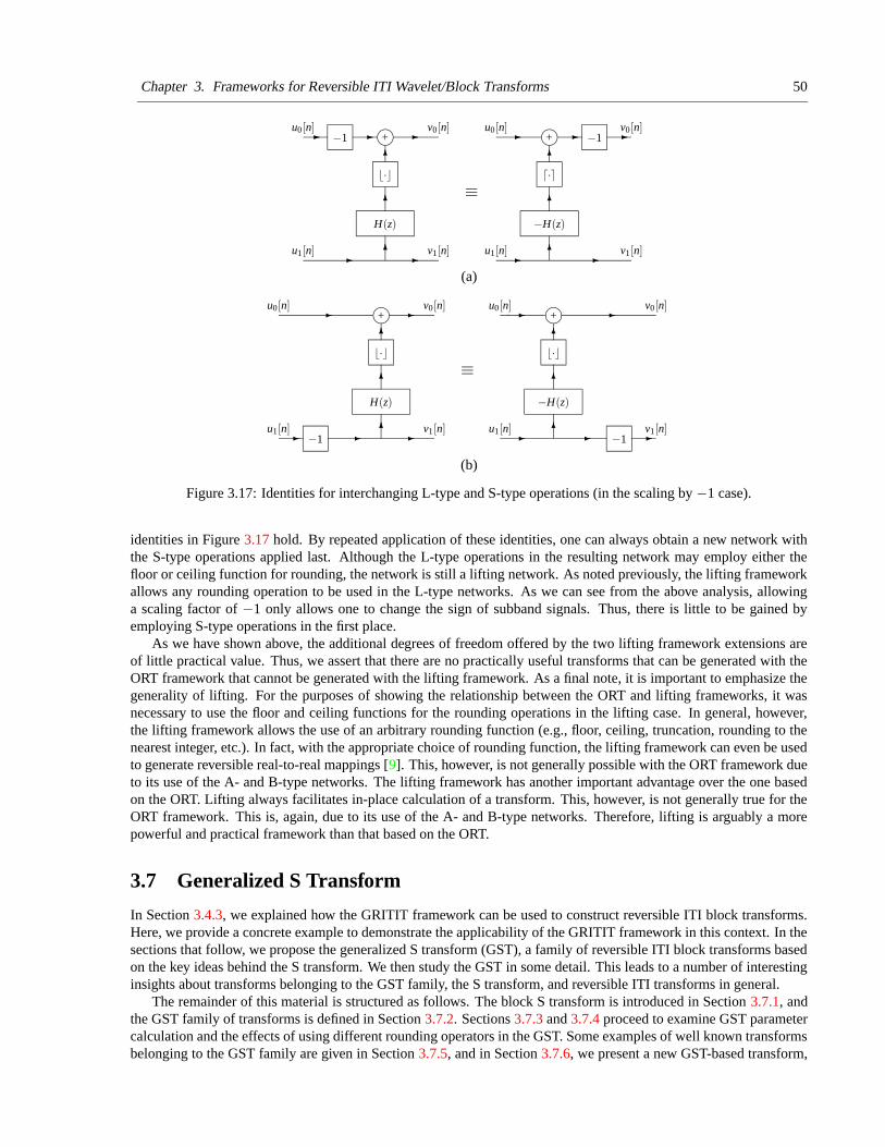
Chapter 3. Frameworks for Reversible ITI Wavelet/Block Transforms 50
j+
b·c
H(z)
−1 j+
d·e
−H(z)
−1
6
6
-
6 -
--
-
6
-
-
6
6
- -
-
v0[n]
v1[n]u1[n]
u0[n]
u1[n]
u0[n] v0[n]
v1[n]
≡
(a)
j+
b·c
H(z)
j+
b·c
−1
−H(z)
−1
6
6
- -
6- --
.
6
- -
--
6
6 -
u0[n] v0[n]
v1[n]u1[n]
≡
v1[n]
v0[n]
u1[n]
u0[n]
(b)
Figure 3.17: Identities for interchanging L-type and S-type operations (in the scaling by −1 case).
identities in Figure 3.17 hold. By repeated application of these identities, one can always obtain a new network withthe S-type operations applied last. Although the L-type operations in the resulting network may employ either thefloor or ceiling function for rounding, the network is still a lifting network. As noted previously, the lifting frameworkallows any rounding operation to be used in the L-type networks. As we can see from the above analysis, allowinga scaling factor of −1 only allows one to change the sign of subband signals. Thus, there is little to be gained byemploying S-type operations in the first place.
As we have shown above, the additional degrees of freedom offered by the two lifting framework extensions areof little practical value. Thus, we assert that there are no practically useful transforms that can be generated with theORT framework that cannot be generated with the lifting framework. As a final note, it is important to emphasize thegenerality of lifting. For the purposes of showing the relationship between the ORT and lifting frameworks, it wasnecessary to use the floor and ceiling functions for the rounding operations in the lifting case. In general, however,the lifting framework allows the use of an arbitrary rounding function (e.g., floor, ceiling, truncation, rounding to thenearest integer, etc.). In fact, with the appropriate choice of rounding function, the lifting framework can even be usedto generate reversible real-to-real mappings [9]. This, however, is not generally possible with the ORT framework dueto its use of the A- and B-type networks. The lifting framework has another important advantage over the one basedon the ORT. Lifting always facilitates in-place calculation of a transform. This, however, is not generally true for theORT framework. This is, again, due to its use of the A- and B-type networks. Therefore, lifting is arguably a morepowerful and practical framework than that based on the ORT.
3.7 Generalized S Transform
In Section 3.4.3, we explained how the GRITIT framework can be used to construct reversible ITI block transforms.Here, we provide a concrete example to demonstrate the applicability of the GRITIT framework in this context. In thesections that follow, we propose the generalized S transform (GST), a family of reversible ITI block transforms basedon the key ideas behind the S transform. We then study the GST in some detail. This leads to a number of interestinginsights about transforms belonging to the GST family, the S transform, and reversible ITI transforms in general.
The remainder of this material is structured as follows. The block S transform is introduced in Section 3.7.1, andthe GST family of transforms is defined in Section 3.7.2. Sections 3.7.3 and 3.7.4 proceed to examine GST parametercalculation and the effects of using different rounding operators in the GST. Some examples of well known transformsbelonging to the GST family are given in Section 3.7.5, and in Section 3.7.6, we present a new GST-based transform,
Chapter 3. Frameworks for Reversible ITI Wavelet/Block Transforms 51
j+
j+
��
��
��
��
�� A
AA
AA
AA
AA
A
12
b ·c−1
6
-
-
- -
6
6
-
?
?-
--
y0
y1
x0
x1
(a)
j+
j+
AAAAAAAAAA�
���������
b ·c
12
−1
6
6
6?
?
- -
- -
-
--
-−
−y1
y0 x0
x1
(b)
Figure 3.18: The block S transform. The networks for the (a) forward and (b) inverse transforms.
and demonstrate its utility for image coding applications.
3.7.1 Block S Transform
In Section 3.3.1, we introduced the S transform, one of the simplest and most ubiquitous reversible ITI wavelettransforms. The S transform is associated with the networks shown earlier in Figure 3.2. By examining these networks,we can see that the polyphase filtering operations of the S transform themselves constitute a simple two-point blocktransform, which we refer to as the block S transform. That is, the block S transform is associated with the networksshown in Figure 3.18, where the networks in Figures 3.18(a) and 3.18(b) correspond to the forward and inversetransforms, respectively. Mathematically, the forward transform maps the integer vector [ x0 x1 ]T to the integer vector[ y0 y1 ]T , as given by
[ y0y1 ] =
[⌊12 (x0+x1)
⌋
x0−x1
]
.
The corresponding inverse transform is given by
[ x0x1 ] =
[ tt−y1
], where t
4= y0 +
⌊12 (y1 +1)
⌋. (3.56)
3.7.2 Generalized S Transform
By examining the block S transform in the context of the GRITIT framework, we are inspired to propose a naturalextension to this transform, which we call the generalized S transform (GST). For convenience in what follows, let usdefine two integer vectors x and y as
x4= [ x0 x1 ... xN−1 ]T and y
4= [ y0 y1 ... yN−1 ]T .
The forward GST is a mapping from x to y of the form
y = Cx+Q((B−I)Cx) , (3.57)
where B is real matrix of the form
B4=
1 b1 b2 ... bN−10 1 0 ... 00 0 1 ... 0...
......
. . ....
0 0 0 ... 1
,
C is a unimodular (i.e., |detC| = 1) integer matrix defined as
C4=
c0,0 c0,1 c0,2 ... c0,N−1c1,0 c1,1 c1,2 ... c1,N−1c2,0 c2,1 c2,2 ... c2,N−1...
......
. . ....
cN−1,0 cN−1,1 cN−1,2 ... cN−1,N−1
,
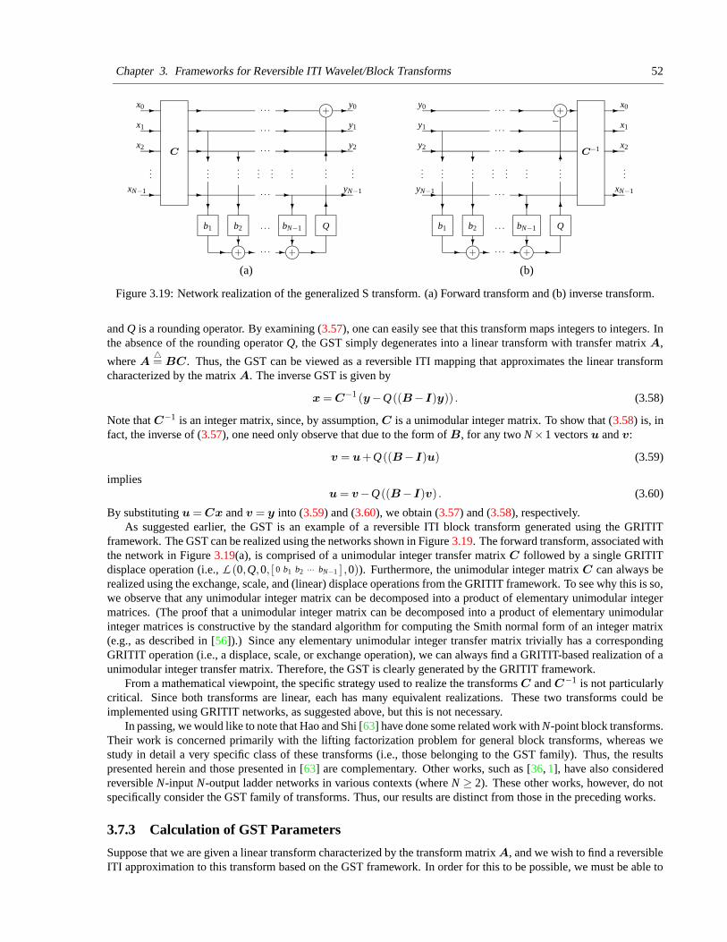
Chapter 3. Frameworks for Reversible ITI Wavelet/Block Transforms 52
j+
Q
j+j+
-
-
-
-
-
- -
-
-
- -
???
?- -
?
6
-- -
6??
-
-
-
- y0
y1
y2C
x2
x1
x0 . . .
. . .
. . .
...
. . .
. . . bN−1b2b1
yN−1. . .
......
......
...
xN−1
......
(a)
j+
Q
j+j+
-
-
-
-
-
-
-
-
-
-
- -
???
?- -
?
6
-- -
? ? 6
−
C−1
x0
x2
x1
. . .
. . .
. . .
y0
y1
y2
. . . bN−1b2b1
xN−1. . .
. . .
yN−1
......
......
......
......
(b)
Figure 3.19: Network realization of the generalized S transform. (a) Forward transform and (b) inverse transform.
and Q is a rounding operator. By examining (3.57), one can easily see that this transform maps integers to integers. Inthe absence of the rounding operator Q, the GST simply degenerates into a linear transform with transfer matrix A,
where A4= BC. Thus, the GST can be viewed as a reversible ITI mapping that approximates the linear transform
characterized by the matrix A. The inverse GST is given by
x = C−1 (y−Q((B−I)y)) . (3.58)
Note that C−1 is an integer matrix, since, by assumption, C is a unimodular integer matrix. To show that (3.58) is, infact, the inverse of (3.57), one need only observe that due to the form of B, for any two N ×1 vectors u and v:
v = u+Q((B−I)u) (3.59)
impliesu = v−Q((B−I)v) . (3.60)
By substituting u = Cx and v = y into (3.59) and (3.60), we obtain (3.57) and (3.58), respectively.As suggested earlier, the GST is an example of a reversible ITI block transform generated using the GRITIT
framework. The GST can be realized using the networks shown in Figure 3.19. The forward transform, associated withthe network in Figure 3.19(a), is comprised of a unimodular integer transfer matrix C followed by a single GRITITdisplace operation (i.e., L (0,Q,0, [ 0 b1 b2 ··· bN−1 ] ,0)). Furthermore, the unimodular integer matrix C can always berealized using the exchange, scale, and (linear) displace operations from the GRITIT framework. To see why this is so,we observe that any unimodular integer matrix can be decomposed into a product of elementary unimodular integermatrices. (The proof that a unimodular integer matrix can be decomposed into a product of elementary unimodularinteger matrices is constructive by the standard algorithm for computing the Smith normal form of an integer matrix(e.g., as described in [56]).) Since any elementary unimodular integer transfer matrix trivially has a correspondingGRITIT operation (i.e., a displace, scale, or exchange operation), we can always find a GRITIT-based realization of aunimodular integer transfer matrix. Therefore, the GST is clearly generated by the GRITIT framework.
From a mathematical viewpoint, the specific strategy used to realize the transforms C and C−1 is not particularlycritical. Since both transforms are linear, each has many equivalent realizations. These two transforms could beimplemented using GRITIT networks, as suggested above, but this is not necessary.
In passing, we would like to note that Hao and Shi [63] have done some related work with N-point block transforms.Their work is concerned primarily with the lifting factorization problem for general block transforms, whereas westudy in detail a very specific class of these transforms (i.e., those belonging to the GST family). Thus, the resultspresented herein and those presented in [63] are complementary. Other works, such as [36, 1], have also consideredreversible N-input N-output ladder networks in various contexts (where N ≥ 2). These other works, however, do notspecifically consider the GST family of transforms. Thus, our results are distinct from those in the preceding works.
3.7.3 Calculation of GST Parameters
Suppose that we are given a linear transform characterized by the transform matrix A, and we wish to find a reversibleITI approximation to this transform based on the GST framework. In order for this to be possible, we must be able to
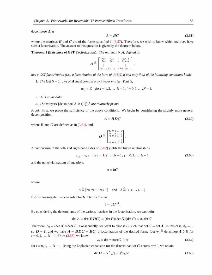
Chapter 3. Frameworks for Reversible ITI Wavelet/Block Transforms 53
decompose A asA = BC (3.61)
where the matrices B and C are of the forms specified in (3.57). Therefore, we wish to know which matrices havesuch a factorization. The answer to this question is given by the theorem below.
Theorem 1 (Existence of GST Factorization). The real matrix A, defined as
A4=
a0,0 a0,1 ... a0,N−1a1,0 a1,1 ... a1,N−1...
.... . .
...aN−1,0 aN−1,1 ... aN−1,N−1
,
has a GST factorization (i.e., a factorization of the form of (3.61)) if and only if all of the following conditions hold:
1. The last N −1 rows of A must contain only integer entries. That is,
ai, j ∈ Z for i = 1,2, . . . ,N −1, j = 0,1, . . . ,N −1.
2. A is unimodular.
3. The integers {detminor(A,0, i)}N−1i=0 are relatively prime.
Proof. First, we prove the sufficiency of the above conditions. We begin by considering the slightly more generaldecomposition
A = BDC (3.62)
where B and C are defined as in (3.61), and
D4=
b0 0 0 ... 00 1 0 ... 00 0 1 ... 0...
......
. . . 00 0 0 0 1
.
A comparison of the left- and right-hand sides of (3.62) yields the trivial relationships
ci, j = ai, j for i = 1,2, . . . ,N −1, j = 0,1, . . . ,N −1 (3.63)
and the nontrivial system of equations
a = bC
where
a4= [ a0,0 a0,1 ... a0,N−1 ] and b
4= [ b0 b1 ... bN−1 ] .
If C is nonsingular, we can solve for b in terms of a as
b = aC−1.
By considering the determinants of the various matrices in the factorization, we can write
detA = det(BDC) = (detB)(detD)(detC) = b0 detC.
Therefore, b0 = (detA)/(detC). Consequently, we want to choose C such that detC = detA. In this case, b0 = 1,
so D = I , and we have A = BDC = BC, a factorization of the desired form. Let wi4= detminor(A,0, i) for
i = 0,1, . . . ,N −1. From (3.63), we knowwi = detminor(C,0, i) (3.64)
for i = 0,1, . . . ,N −1. Using the Laplacian expansion for the determinant of C across row 0, we obtain
detC = ∑N−1i=0 (−1)ic0,iwi. (3.65)
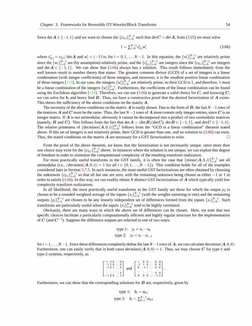
Chapter 3. Frameworks for Reversible ITI Wavelet/Block Transforms 54
Since detA ∈ {−1,1} and we want to choose the {c0,i}N−1i=0 such that detC = detA, from (3.65) we must solve
1 = ∑N−1i=0 c′0,iw
′i (3.66)
where c′0,i = c0,i/detA and w′i = (−1)iwi for i = 0,1, . . . ,N − 1. In this equation, the {w′
i}N−1i=0 are relatively prime
since the {wi}N−1i=0 are (by assumption) relatively prime, and the {c′0,i}N−1
i=0 are integers since the {c0,i}N−1i=0 are integers
and detA ∈ {−1,1}. We can show that (3.66) always has a solution. This result follows immediately from thewell known result in number theory that states: The greatest common divisor (GCD) of a set of integers is a linearcombination (with integer coefficients) of those integers, and moreover, it is the smallest positive linear combinationof those integers [121]. In our case, the integers {w′
i}N−1i=0 are relatively prime, so their GCD is 1, and therefore, 1 must
be a linear combination of the integers {w′i}N−1
i=0 . Furthermore, the coefficients of the linear combination can be foundusing the Euclidean algorithm [121]. Therefore, we can use (3.66) to generate a valid choice for C, and knowing C,we can solve for b, and hence find B. Thus, we have a constructive proof that the desired factorization of A exists.This shows the sufficiency of the above conditions on the matrix A.
The necessity of the above conditions on the matrix A is easily shown. Due to the form of B, the last N−1 rows ofthe matrices A and C must be the same. Thus, the last N−1 rows of A must contain only integer entries, since C is aninteger matrix. If A is not unimodular, obviously it cannot be decomposed into a product of two unimodular matrices(namely, B and C). This follows from the fact that detA = (detB)(detC), detB ∈ {−1,1}, and detC ∈ {−1,1}.The relative primeness of {detminor(A,0, i)}N−1
i=0 follows from the “GCD is a linear combination” theorem statedabove. If this set of integers is not relatively prime, their GCD is greater than one, and no solution to (3.66) can exist.Thus, the stated conditions on the matrix A are necessary for a GST factorization to exist.
From the proof of the above theorem, we know that the factorization is not necessarily unique, since more thanone choice may exist for the {c0,i}N−1
i=0 above. In instances where the solution is not unique, we can exploit this degreeof freedom in order to minimize the computational complexity of the resulting transform realization.
For most practically useful transforms in the GST family, it is often the case that {minor(A,0, i)}N−1i=0 are all
unimodular (i.e., |detminor(A,0, i)| = 1 for all i ∈ {0,1, . . . ,N − 1}). This condition holds for all of the examplesconsidered later in Section 3.7.5. In such instances, the most useful GST factorizations are often obtained by choosingthe unknowns {c0,i}N−1
i=0 so that all but one are zero, with the remaining unknown being chosen as either −1 or 1 inorder to satisfy (3.66). In this way, we can readily obtain N distinct GST factorizations of A which typically yield lowcomplexity transform realizations.
In all likelihood, the most practically useful transforms in the GST family are those for which the output y0 ischosen to be a rounded weighted average of the inputs {xi}N−1
i=0 (with the weights summing to one) and the remainingoutputs {yi}N−1
i=1 are chosen to be any linearly independent set of differences formed from the inputs {xi}N−1i=0 . Such
transforms are particularly useful when the inputs {xi}N−1i=0 tend to be highly correlated.
Obviously, there are many ways in which the above set of differences can be chosen. Here, we note that twospecific choices facilitate a particularly computationally efficient and highly regular structure for the implementationof C (and C−1). Suppose the difference outputs are selected in one of two ways:
type 1: yi = xi − x0
type 2: yi = xi − xi−1
for i = 1, . . . ,N−1. Since these differences completely define the last N−1 rows of A, we can calculate detminor(A,0,0).Furthermore, one can easily verify that in both cases detminor(A,0,0) = 1. Thus, we may choose C for type-1 andtype-2 systems, respectively, as
1 0 0 ... 0−1 1 0 ... 0−1 0 1 ... 0...
......
. . . 0−1 0 0 ... 1
and
1 0 0 ... 0 0−1 1 0 ... 0 00 −1 1 ... 0 0...
......
. . . 0 00 0 0 ... −1 1
.
Furthermore, we can show that the corresponding solutions for B are, respectively, given by
type 1: bi = a0,i
type 2: bi = ∑N−1k=i a0,k
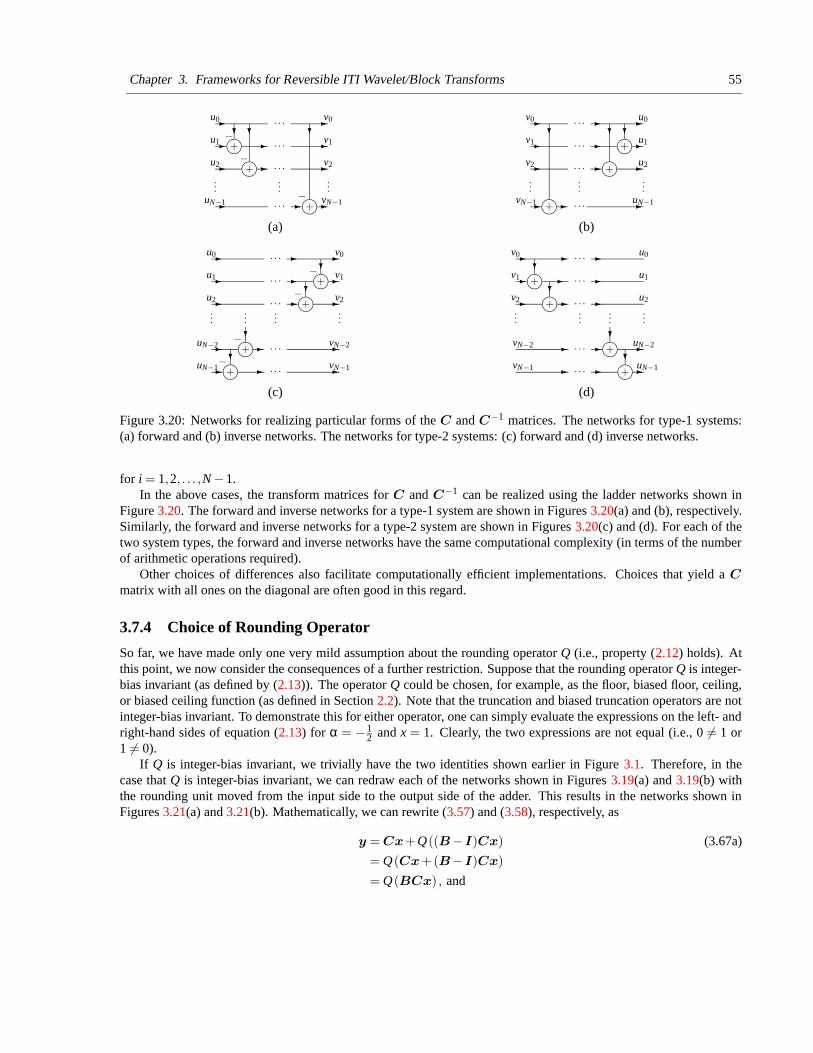
Chapter 3. Frameworks for Reversible ITI Wavelet/Block Transforms 55
j+
j+
j+
?-
-
-
?
-
-
-
-
--
-
-?
u0
u1
u2
−
−
...
v2
v1
v0
...
. . .
. . .
. . .
... − vN−1uN−1 . . .
(a)
j+
j+
j+
-
-??
-
-
-
-?
-
-
-
- - -
u2
u1
u0
...
. . .
. . .
. . .v2
v1
v0
......
. . . uN−1vN−1
(b)
j+
j+
j+
j+
-
-
-
-
-
-
-?
?
-
-
-
-
-
-
-
-
?
?
. . .
. . .
. . .
. . .
. . .
vN−2
vN−1uN−1
uN−2
...
u2
u1
u0
......
−
−
v0
v1
v2
...
−
−
(c)
j+
j+
j+
j+-
-
--
-
-
-
-
--
-?
?
-
-?
?-
-
. . .
u0
u1
u2
v0
v1
...
. . .
. . .
. . .
. . .
...
uN−2
......
v2
vN−2
vN−1 uN−1
(d)
Figure 3.20: Networks for realizing particular forms of the C and C−1 matrices. The networks for type-1 systems:(a) forward and (b) inverse networks. The networks for type-2 systems: (c) forward and (d) inverse networks.
for i = 1,2, . . . ,N −1.In the above cases, the transform matrices for C and C−1 can be realized using the ladder networks shown in
Figure 3.20. The forward and inverse networks for a type-1 system are shown in Figures 3.20(a) and (b), respectively.Similarly, the forward and inverse networks for a type-2 system are shown in Figures 3.20(c) and (d). For each of thetwo system types, the forward and inverse networks have the same computational complexity (in terms of the numberof arithmetic operations required).
Other choices of differences also facilitate computationally efficient implementations. Choices that yield a C
matrix with all ones on the diagonal are often good in this regard.
3.7.4 Choice of Rounding Operator
So far, we have made only one very mild assumption about the rounding operator Q (i.e., property (2.12) holds). Atthis point, we now consider the consequences of a further restriction. Suppose that the rounding operator Q is integer-bias invariant (as defined by (2.13)). The operator Q could be chosen, for example, as the floor, biased floor, ceiling,or biased ceiling function (as defined in Section 2.2). Note that the truncation and biased truncation operators are notinteger-bias invariant. To demonstrate this for either operator, one can simply evaluate the expressions on the left- andright-hand sides of equation (2.13) for α = − 1
2 and x = 1. Clearly, the two expressions are not equal (i.e., 0 6= 1 or1 6= 0).
If Q is integer-bias invariant, we trivially have the two identities shown earlier in Figure 3.1. Therefore, in thecase that Q is integer-bias invariant, we can redraw each of the networks shown in Figures 3.19(a) and 3.19(b) withthe rounding unit moved from the input side to the output side of the adder. This results in the networks shown inFigures 3.21(a) and 3.21(b). Mathematically, we can rewrite (3.57) and (3.58), respectively, as
y = Cx+Q((B−I)Cx) (3.67a)
= Q(Cx+(B−I)Cx)
= Q(BCx) , and
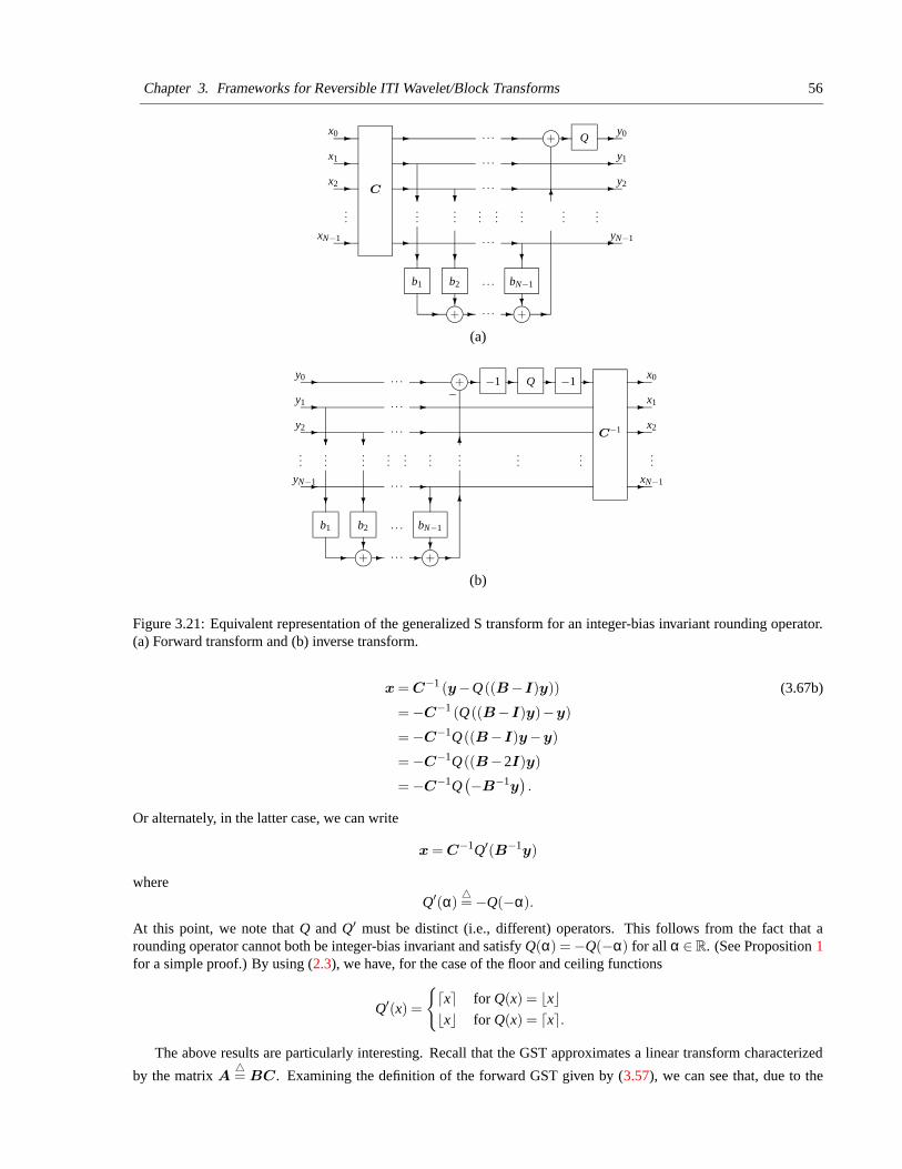
Chapter 3. Frameworks for Reversible ITI Wavelet/Block Transforms 56
j+j+
j+ Q-
-
- -
-
-
-
???
?- -
?
- -
??
-
-
-
-
6
- -
-
-
-
-
Cx2
x1
x0 . . .
. . .
. . .
...
. . .
. . . bN−1b2b1
. . .
......
......
...
xN−1
......
y0
y1
y2
yN−1
(a)
j+j+
j+
6-
-
-
-
-
-
-
???
?- -
?
- -
? ?
-
y2
6. . .
-
-
-
-
- - - -
b2
...
. . .
. . .
. . .
y0
y1
......
bN−1
−1
b1
. . .
. . .
yN−1
......
Q
......
x2
−1x0
x1
xN−1
...
C−1
......
−
(b)
Figure 3.21: Equivalent representation of the generalized S transform for an integer-bias invariant rounding operator.(a) Forward transform and (b) inverse transform.
x = C−1 (y−Q((B−I)y)) (3.67b)
= −C−1 (Q((B−I)y)−y)
= −C−1Q((B−I)y−y)
= −C−1Q((B−2I)y)
= −C−1Q(−B−1y
).
Or alternately, in the latter case, we can write
x = C−1Q′(B−1y)
whereQ′(α)
4= −Q(−α).
At this point, we note that Q and Q′ must be distinct (i.e., different) operators. This follows from the fact that arounding operator cannot both be integer-bias invariant and satisfy Q(α) = −Q(−α) for all α ∈ R. (See Proposition 1for a simple proof.) By using (2.3), we have, for the case of the floor and ceiling functions
Q′(x) =
{
dxe for Q(x) = bxcbxc for Q(x) = dxe.
The above results are particularly interesting. Recall that the GST approximates a linear transform characterized
by the matrix A4= BC. Examining the definition of the forward GST given by (3.57), we can see that, due to the
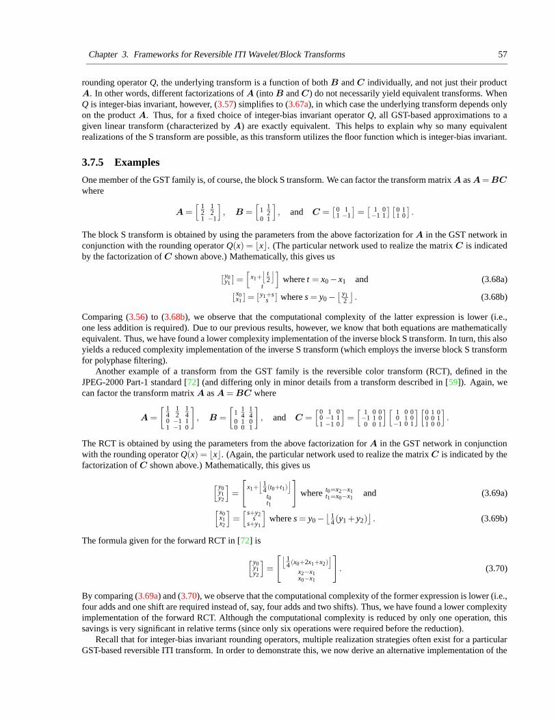
Chapter 3. Frameworks for Reversible ITI Wavelet/Block Transforms 57
rounding operator Q, the underlying transform is a function of both B and C individually, and not just their productA. In other words, different factorizations of A (into B and C) do not necessarily yield equivalent transforms. WhenQ is integer-bias invariant, however, (3.57) simplifies to (3.67a), in which case the underlying transform depends onlyon the product A. Thus, for a fixed choice of integer-bias invariant operator Q, all GST-based approximations to agiven linear transform (characterized by A) are exactly equivalent. This helps to explain why so many equivalentrealizations of the S transform are possible, as this transform utilizes the floor function which is integer-bias invariant.
3.7.5 Examples
One member of the GST family is, of course, the block S transform. We can factor the transform matrix A as A = BC
where
A =[ 1
212
1 −1
]
, B =[
1 12
0 1
]
, and C =[
0 11 −1
]=[
1 0−1 1
][0 11 0
].
The block S transform is obtained by using the parameters from the above factorization for A in the GST network inconjunction with the rounding operator Q(x) = bxc. (The particular network used to realize the matrix C is indicatedby the factorization of C shown above.) Mathematically, this gives us
[ y0y1 ] =
[x1+
⌊t2
⌋
t
]
where t = x0 − x1 and (3.68a)
[ x0x1 ] = [ y1+s
s ] where s = y0 −⌊ y1
2
⌋. (3.68b)
Comparing (3.56) to (3.68b), we observe that the computational complexity of the latter expression is lower (i.e.,one less addition is required). Due to our previous results, however, we know that both equations are mathematicallyequivalent. Thus, we have found a lower complexity implementation of the inverse block S transform. In turn, this alsoyields a reduced complexity implementation of the inverse S transform (which employs the inverse block S transformfor polyphase filtering).
Another example of a transform from the GST family is the reversible color transform (RCT), defined in theJPEG-2000 Part-1 standard [72] (and differing only in minor details from a transform described in [59]). Again, wecan factor the transform matrix A as A = BC where
A =
[ 14
12
14
0 −1 11 −1 0
]
, B =
[1 1
414
0 1 00 0 1
]
, and C =[0 1 0
0 −1 11 −1 0
]
=[
1 0 0−1 1 00 0 1
][1 0 00 1 0−1 0 1
][0 1 00 0 11 0 0
]
.
The RCT is obtained by using the parameters from the above factorization for A in the GST network in conjunctionwith the rounding operator Q(x) = bxc. (Again, the particular network used to realize the matrix C is indicated by thefactorization of C shown above.) Mathematically, this gives us
[ y0y1y2
]
=
[
x1+⌊
14 (t0+t1)
⌋
t0t1
]
where t0=x2−x1t1=x0−x1
and (3.69a)
[ x0x1x2
]
=[ s+y2
ss+y1
]
where s = y0 −⌊
14 (y1 + y2)
⌋. (3.69b)
The formula given for the forward RCT in [72] is
[ y0y1y2
]
=
[⌊14 (x0+2x1+x2)
⌋
x2−x1x0−x1
]
. (3.70)
By comparing (3.69a) and (3.70), we observe that the computational complexity of the former expression is lower (i.e.,four adds and one shift are required instead of, say, four adds and two shifts). Thus, we have found a lower complexityimplementation of the forward RCT. Although the computational complexity is reduced by only one operation, thissavings is very significant in relative terms (since only six operations were required before the reduction).
Recall that for integer-bias invariant rounding operators, multiple realization strategies often exist for a particularGST-based reversible ITI transform. In order to demonstrate this, we now derive an alternative implementation of the
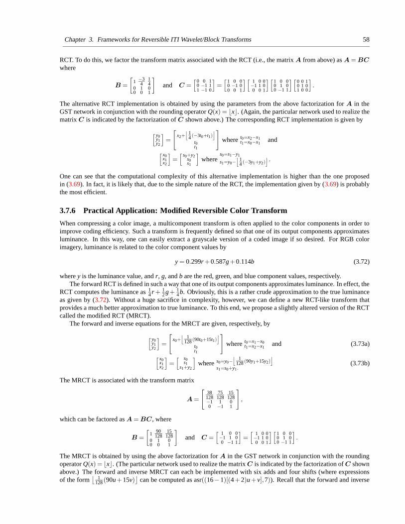
Chapter 3. Frameworks for Reversible ITI Wavelet/Block Transforms 58
RCT. To do this, we factor the transform matrix associated with the RCT (i.e., the matrix A from above) as A = BC
where
B =
[1 −3
414
0 1 00 0 1
]
and C =[ 0 0 1
0 −1 11 −1 0
]
=[
1 0 00 −1 00 0 1
][1 0 0−1 1 00 0 1
][1 0 00 1 00 −1 1
][0 0 10 1 01 0 0
]
.
The alternative RCT implementation is obtained by using the parameters from the above factorization for A in theGST network in conjunction with the rounding operator Q(x) = bxc. (Again, the particular network used to realize thematrix C is indicated by the factorization of C shown above.) The corresponding RCT implementation is given by
[ y0y1y2
]
=
[
x2+⌊
14 (−3t0+t1)
⌋
t0t1
]
where t0=x2−x1t1=x0−x1
and
[ x0x1x2
]
=[ s0+y2
s0s1
]
wheres0=s1−y1
s1=y0−⌊
14 (−3y1+y2)
⌋.
One can see that the computational complexity of this alternative implementation is higher than the one proposedin (3.69). In fact, it is likely that, due to the simple nature of the RCT, the implementation given by (3.69) is probablythe most efficient.
3.7.6 Practical Application: Modified Reversible Color Transform
When compressing a color image, a multicomponent transform is often applied to the color components in order toimprove coding efficiency. Such a transform is frequently defined so that one of its output components approximatesluminance. In this way, one can easily extract a grayscale version of a coded image if so desired. For RGB colorimagery, luminance is related to the color component values by
y = 0.299r +0.587g+0.114b (3.72)
where y is the luminance value, and r, g, and b are the red, green, and blue component values, respectively.The forward RCT is defined in such a way that one of its output components approximates luminance. In effect, the
RCT computes the luminance as 14 r + 1
2 g+ 14 b. Obviously, this is a rather crude approximation to the true luminance
as given by (3.72). Without a huge sacrifice in complexity, however, we can define a new RCT-like transform thatprovides a much better approximation to true luminance. To this end, we propose a slightly altered version of the RCTcalled the modified RCT (MRCT).
The forward and inverse equations for the MRCT are given, respectively, by
[ y0y1y2
]
=
[
x0+⌊
1128 (90t0+15t1)
⌋
t0t1
]
where t0=x1−x0t1=x2−x1
and (3.73a)
[ x0x1x2
]
=[ s0
s1s1+y2
]
where s0=y0−⌊
1128 (90y1+15y2)
⌋
s1=s0+y1.(3.73b)
The MRCT is associated with the transform matrix
A =
[38
12875
12815
128−1 1 00 −1 1
]
,
which can be factored as A = BC, where
B =
[1 90
12815
1280 1 00 0 1
]
and C =[ 1 0 0−1 1 00 −1 1
]
=[
1 0 0−1 1 00 0 1
][1 0 00 1 00 −1 1
]
.
The MRCT is obtained by using the above factorization for A in the GST network in conjunction with the roundingoperator Q(x) = bxc. (The particular network used to realize the matrix C is indicated by the factorization of C shownabove.) The forward and inverse MRCT can each be implemented with six adds and four shifts (where expressionsof the form
⌊1
128 (90u+15v)⌋
can be computed as asr((16−1)[(4 + 2)u + v],7)). Recall that the forward and inverse
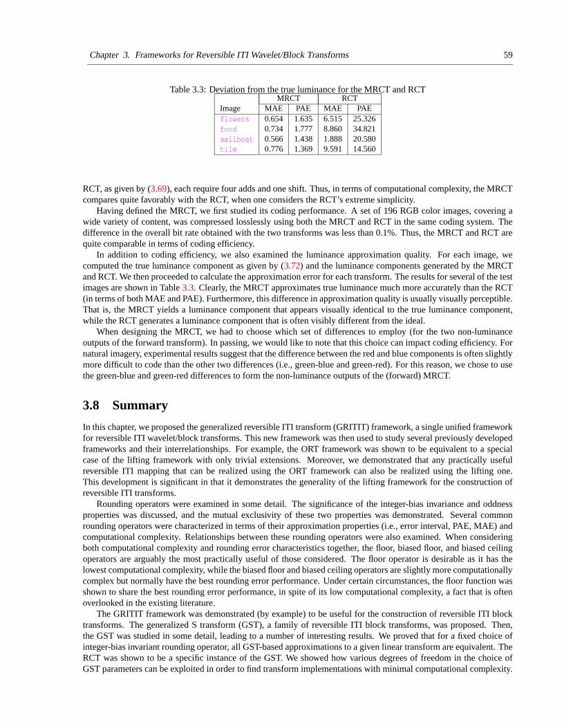
Chapter 3. Frameworks for Reversible ITI Wavelet/Block Transforms 59
Table 3.3: Deviation from the true luminance for the MRCT and RCTMRCT RCT
Image MAE PAE MAE PAEflowers 0.654 1.635 6.515 25.326food 0.734 1.777 8.860 34.821sailboat 0.566 1.438 1.888 20.580tile 0.776 1.369 9.591 14.560
RCT, as given by (3.69), each require four adds and one shift. Thus, in terms of computational complexity, the MRCTcompares quite favorably with the RCT, when one considers the RCT’s extreme simplicity.
Having defined the MRCT, we first studied its coding performance. A set of 196 RGB color images, covering awide variety of content, was compressed losslessly using both the MRCT and RCT in the same coding system. Thedifference in the overall bit rate obtained with the two transforms was less than 0.1%. Thus, the MRCT and RCT arequite comparable in terms of coding efficiency.
In addition to coding efficiency, we also examined the luminance approximation quality. For each image, wecomputed the true luminance component as given by (3.72) and the luminance components generated by the MRCTand RCT. We then proceeded to calculate the approximation error for each transform. The results for several of the testimages are shown in Table 3.3. Clearly, the MRCT approximates true luminance much more accurately than the RCT(in terms of both MAE and PAE). Furthermore, this difference in approximation quality is usually visually perceptible.That is, the MRCT yields a luminance component that appears visually identical to the true luminance component,while the RCT generates a luminance component that is often visibly different from the ideal.
When designing the MRCT, we had to choose which set of differences to employ (for the two non-luminanceoutputs of the forward transform). In passing, we would like to note that this choice can impact coding efficiency. Fornatural imagery, experimental results suggest that the difference between the red and blue components is often slightlymore difficult to code than the other two differences (i.e., green-blue and green-red). For this reason, we chose to usethe green-blue and green-red differences to form the non-luminance outputs of the (forward) MRCT.
3.8 Summary
In this chapter, we proposed the generalized reversible ITI transform (GRITIT) framework, a single unified frameworkfor reversible ITI wavelet/block transforms. This new framework was then used to study several previously developedframeworks and their interrelationships. For example, the ORT framework was shown to be equivalent to a specialcase of the lifting framework with only trivial extensions. Moreover, we demonstrated that any practically usefulreversible ITI mapping that can be realized using the ORT framework can also be realized using the lifting one.This development is significant in that it demonstrates the generality of the lifting framework for the construction ofreversible ITI transforms.
Rounding operators were examined in some detail. The significance of the integer-bias invariance and oddnessproperties was discussed, and the mutual exclusivity of these two properties was demonstrated. Several commonrounding operators were characterized in terms of their approximation properties (i.e., error interval, PAE, MAE) andcomputational complexity. Relationships between these rounding operators were also examined. When consideringboth computational complexity and rounding error characteristics together, the floor, biased floor, and biased ceilingoperators are arguably the most practically useful of those considered. The floor operator is desirable as it has thelowest computational complexity, while the biased floor and biased ceiling operators are slightly more computationallycomplex but normally have the best rounding error performance. Under certain circumstances, the floor function wasshown to share the best rounding error performance, in spite of its low computational complexity, a fact that is oftenoverlooked in the existing literature.
The GRITIT framework was demonstrated (by example) to be useful for the construction of reversible ITI blocktransforms. The generalized S transform (GST), a family of reversible ITI block transforms, was proposed. Then,the GST was studied in some detail, leading to a number of interesting results. We proved that for a fixed choice ofinteger-bias invariant rounding operator, all GST-based approximations to a given linear transform are equivalent. TheRCT was shown to be a specific instance of the GST. We showed how various degrees of freedom in the choice ofGST parameters can be exploited in order to find transform implementations with minimal computational complexity.

Chapter 3. Frameworks for Reversible ITI Wavelet/Block Transforms 60
Moreover, the GST framework was used as a means to derive reduced complexity implementations of the S transformand RCT. A new transform belonging to the GST family, called the MRCT, was introduced, and shown to be practicallyuseful for image coding applications. Due to its utility, the GST family of transforms will no doubt continue to proveuseful in both present and future signal coding applications.
When I despair, I remember that all through history, the way of truth and lovehas always won. There have been murderers and tyrants, and for a time theycan seem invincible. But in the end they always fall. Think of it, always.
—Mohandas Karamchand Gandhi (1869–1948)
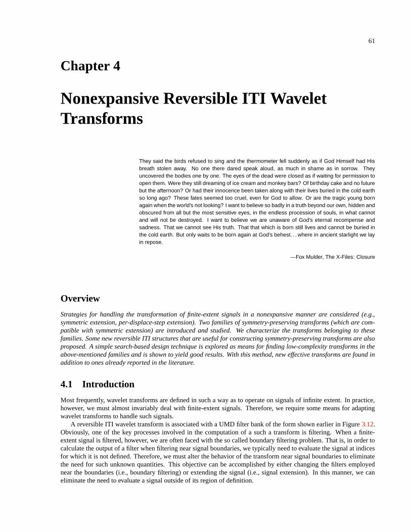
61
Chapter 4
Nonexpansive Reversible ITI WaveletTransforms
They said the birds refused to sing and the thermometer fell suddenly as if God Himself had Hisbreath stolen away. No one there dared speak aloud, as much in shame as in sorrow. Theyuncovered the bodies one by one. The eyes of the dead were closed as if waiting for permission toopen them. Were they still dreaming of ice cream and monkey bars? Of birthday cake and no futurebut the afternoon? Or had their innocence been taken along with their lives buried in the cold earthso long ago? These fates seemed too cruel, even for God to allow. Or are the tragic young bornagain when the world’s not looking? I want to believe so badly in a truth beyond our own, hidden andobscured from all but the most sensitive eyes, in the endless procession of souls, in what cannotand will not be destroyed. I want to believe we are unaware of God’s eternal recompense andsadness. That we cannot see His truth. That that which is born still lives and cannot be buried inthe cold earth. But only waits to be born again at God’s behest. . . where in ancient starlight we layin repose.
—Fox Mulder, The X-Files: Closure
Overview
Strategies for handling the transformation of finite-extent signals in a nonexpansive manner are considered (e.g.,symmetric extension, per-displace-step extension). Two families of symmetry-preserving transforms (which are com-patible with symmetric extension) are introduced and studied. We characterize the transforms belonging to thesefamilies. Some new reversible ITI structures that are useful for constructing symmetry-preserving transforms are alsoproposed. A simple search-based design technique is explored as means for finding low-complexity transforms in theabove-mentioned families and is shown to yield good results. With this method, new effective transforms are found inaddition to ones already reported in the literature.
4.1 Introduction
Most frequently, wavelet transforms are defined in such a way as to operate on signals of infinite extent. In practice,however, we must almost invariably deal with finite-extent signals. Therefore, we require some means for adaptingwavelet transforms to handle such signals.
A reversible ITI wavelet transform is associated with a UMD filter bank of the form shown earlier in Figure 3.12.Obviously, one of the key processes involved in the computation of a such a transform is filtering. When a finite-extent signal is filtered, however, we are often faced with the so called boundary filtering problem. That is, in order tocalculate the output of a filter when filtering near signal boundaries, we typically need to evaluate the signal at indicesfor which it is not defined. Therefore, we must alter the behavior of the transform near signal boundaries to eliminatethe need for such unknown quantities. This objective can be accomplished by either changing the filters employednear the boundaries (i.e., boundary filtering) or extending the signal (i.e., signal extension). In this manner, we caneliminate the need to evaluate a signal outside of its region of definition.
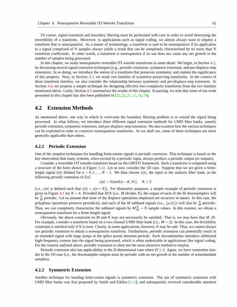
Chapter 4. Nonexpansive Reversible ITI Wavelet Transforms 62
Of course, signal extension and boundary filtering must be performed with care in order to avoid destroying theinvertibility of a transform. Moreover, in applications such as signal coding, we almost always want to employ atransform that is nonexpansive. As a matter of terminology, a transform is said to be nonexpansive if its applicationto a signal comprised of N samples always yields a result that can be completely characterized by no more than Ntransform coefficients. In other words, a transform is nonexpansive if its use does not cause any net growth in thenumber of samples being processed.
In this chapter, we study nonexpansive reversible ITI wavelet transforms in some detail. We begin, in Section 4.2,by discussing several signal extension techniques (e.g., periodic extension, symmetric extension, and per-displace-stepextension). In so doing, we introduce the notion of a transform that preserves symmetry, and explain the significanceof this property. Next, in Section 4.3, we study two families of symmetry-preserving transforms. In the context ofthese transform families, we also consider the relationship between symmetric and per-displace-step extension. InSection 4.4, we propose a simple technique for designing effective low-complexity transforms from the two familiesmentioned above. Lastly, Section 4.5 summarizes the results of this chapter. In passing, we note that some of our workpresented in this chapter has also been published in [20, 22, 21, 12, 16, 10].
4.2 Extension Methods
As mentioned above, one way in which to overcome the boundary filtering problem is to extend the signal beingprocessed. In what follows, we introduce three different signal extension methods for UMD filter banks, namelyperiodic extension, symmetric extension, and per-displace-step extension. We also examine how the various techniquescan be exploited in order to construct nonexpansive transforms. As we shall see, some of these techniques are moregenerally applicable than others.
4.2.1 Periodic Extension
One of the simplest techniques for handling finite-extent signals is periodic extension. This technique is based on thekey observation that many systems, when excited by a periodic input, always produce a periodic output (or outputs).
Consider a reversible ITI wavelet transform based on the GRITIT framework. Such a transform is computed usinga structure of the form shown in Figure 3.12. Let us now consider the 1D case. Suppose that we are given a finite-length signal x[n] defined for n = 0,1, . . . ,N − 1. We then choose x[n], the input to the analysis filter bank, as thefollowing periodic extension of x[n]:
x[n] = x[mod(n−K,N)], K ∈ Z
(i.e., x[n] is defined such that x[n] = x[n + N]). For illustrative purposes, a simple example of periodic extension isgiven in Figure 4.1 for N = 4. Provided that M|N (i.e., M divides N), the output of each of the M downsamplers willbe N
M periodic. Let us assume that none of the displace operations employed are recursive in nature. In this case, thepolyphase operations preserve periodicity, and each of the M subband signals (i.e., {yi[n]}) will also be N
M -periodic.Thus, we can completely characterize the subband signals by M N
M = N sample values. In this manner, we obtain anonexpansive transform for a finite-length signal.
Obviously, the above constraint on M and N may not necessarily be satisfied. That is, we may have that M 6 |N.For example, consider a transform based on a two-channel UMD filter bank (i.e., M = 2). In this case, the divisibilityconstraint is satisfied only if N is even. Clearly, in some applications, however, N may be odd. Thus, we cannot alwaysuse periodic extension to obtain a nonexpansive transform. Furthermore, periodic extension can potentially result inan extended signal with large jumps at the splice points between periods. Such discontinuities introduce additionalhigh-frequency content into the signal being processed, which is often undesirable in applications like signal coding.For the reasons outlined above, periodic extension is often not the most attractive method to employ.
Periodic extension also has applicability in the D-dimensional case where D ≥ 2. Again, we have constraints sim-ilar to the 1D case (i.e., the downsampler outputs must be periodic with no net growth in the number of nonredundantsamples).
4.2.2 Symmetric Extension
Another technique for handing finite-extent signals is symmetric extension. The use of symmetric extension withUMD filter banks was first proposed by Smith and Eddins [122], and subsequently received considerable attention
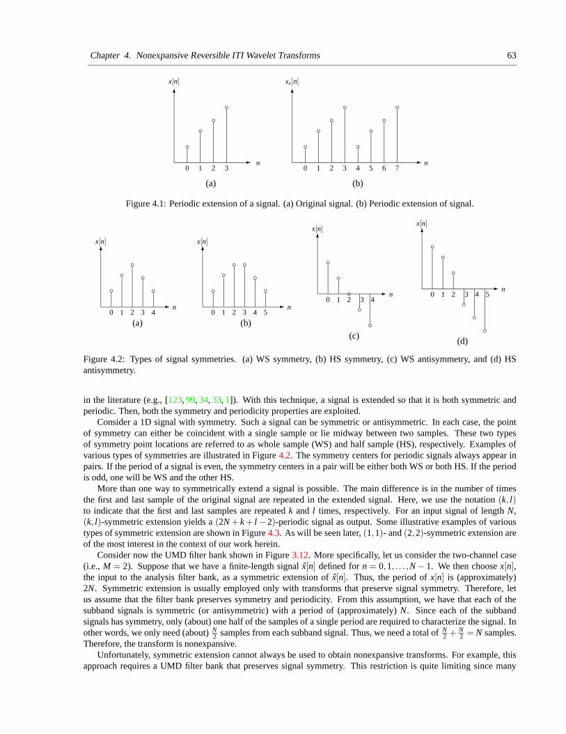
Chapter 4. Nonexpansive Reversible ITI Wavelet Transforms 63
b
b
b
b
b
b
bb
b
bb
b
-
6 6
-20 1 4 5 760 1 2 3
(a)
x[n]
n
xs[n]
3n
(b)
Figure 4.1: Periodic extension of a signal. (a) Original signal. (b) Periodic extension of signal.
x[n]
n
bb
b
b b
6
-0 1 2 3 4
(a)
x[n]
n
bb
b bb
b6
-0 1 2 3 4 5
(b)
x[n]
nb
b
b
b
b
-
6
0 1 2 3 4
(c)
x[n]
n
b
b
b
b
b
b
6
-0 1 2 3 4 5
(d)
Figure 4.2: Types of signal symmetries. (a) WS symmetry, (b) HS symmetry, (c) WS antisymmetry, and (d) HSantisymmetry.
in the literature (e.g., [123, 99, 34, 33, 1]). With this technique, a signal is extended so that it is both symmetric andperiodic. Then, both the symmetry and periodicity properties are exploited.
Consider a 1D signal with symmetry. Such a signal can be symmetric or antisymmetric. In each case, the pointof symmetry can either be coincident with a single sample or lie midway between two samples. These two typesof symmetry point locations are referred to as whole sample (WS) and half sample (HS), respectively. Examples ofvarious types of symmetries are illustrated in Figure 4.2. The symmetry centers for periodic signals always appear inpairs. If the period of a signal is even, the symmetry centers in a pair will be either both WS or both HS. If the periodis odd, one will be WS and the other HS.
More than one way to symmetrically extend a signal is possible. The main difference is in the number of timesthe first and last sample of the original signal are repeated in the extended signal. Here, we use the notation (k, l)to indicate that the first and last samples are repeated k and l times, respectively. For an input signal of length N,(k, l)-symmetric extension yields a (2N + k + l − 2)-periodic signal as output. Some illustrative examples of varioustypes of symmetric extension are shown in Figure 4.3. As will be seen later, (1,1)- and (2,2)-symmetric extension areof the most interest in the context of our work herein.
Consider now the UMD filter bank shown in Figure 3.12. More specifically, let us consider the two-channel case(i.e., M = 2). Suppose that we have a finite-length signal x[n] defined for n = 0,1, . . . ,N − 1. We then choose x[n],the input to the analysis filter bank, as a symmetric extension of x[n]. Thus, the period of x[n] is (approximately)2N. Symmetric extension is usually employed only with transforms that preserve signal symmetry. Therefore, letus assume that the filter bank preserves symmetry and periodicity. From this assumption, we have that each of thesubband signals is symmetric (or antisymmetric) with a period of (approximately) N. Since each of the subbandsignals has symmetry, only (about) one half of the samples of a single period are required to characterize the signal. Inother words, we only need (about) N
2 samples from each subband signal. Thus, we need a total of N2 + N
2 = N samples.Therefore, the transform is nonexpansive.
Unfortunately, symmetric extension cannot always be used to obtain nonexpansive transforms. For example, thisapproach requires a UMD filter bank that preserves signal symmetry. This restriction is quite limiting since many
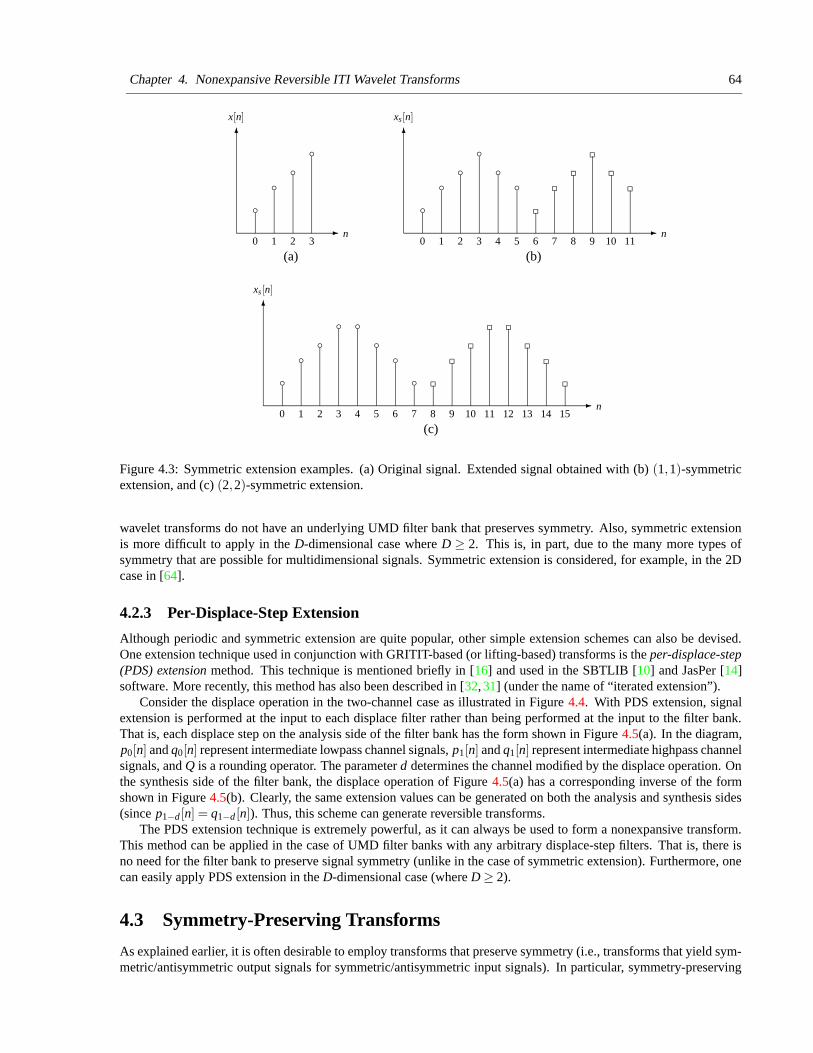
Chapter 4. Nonexpansive Reversible ITI Wavelet Transforms 64
b
b
bb
-
6
0 1 2 3
x[n]
n
(a)
b
b
b
bb
b
-
6
20 1 4 5 7 9 118 106
xs[n]
3n
(b)
b
b
b
b bb
b
b
6
-20 1 4 5 7 9 118 106
xs[n]
3 12 13 14 15n
(c)
Figure 4.3: Symmetric extension examples. (a) Original signal. Extended signal obtained with (b) (1,1)-symmetricextension, and (c) (2,2)-symmetric extension.
wavelet transforms do not have an underlying UMD filter bank that preserves symmetry. Also, symmetric extensionis more difficult to apply in the D-dimensional case where D ≥ 2. This is, in part, due to the many more types ofsymmetry that are possible for multidimensional signals. Symmetric extension is considered, for example, in the 2Dcase in [64].
4.2.3 Per-Displace-Step Extension
Although periodic and symmetric extension are quite popular, other simple extension schemes can also be devised.One extension technique used in conjunction with GRITIT-based (or lifting-based) transforms is the per-displace-step(PDS) extension method. This technique is mentioned briefly in [16] and used in the SBTLIB [10] and JasPer [14]software. More recently, this method has also been described in [32, 31] (under the name of “iterated extension”).
Consider the displace operation in the two-channel case as illustrated in Figure 4.4. With PDS extension, signalextension is performed at the input to each displace filter rather than being performed at the input to the filter bank.That is, each displace step on the analysis side of the filter bank has the form shown in Figure 4.5(a). In the diagram,p0[n] and q0[n] represent intermediate lowpass channel signals, p1[n] and q1[n] represent intermediate highpass channelsignals, and Q is a rounding operator. The parameter d determines the channel modified by the displace operation. Onthe synthesis side of the filter bank, the displace operation of Figure 4.5(a) has a corresponding inverse of the formshown in Figure 4.5(b). Clearly, the same extension values can be generated on both the analysis and synthesis sides(since p1−d [n] = q1−d [n]). Thus, this scheme can generate reversible transforms.
The PDS extension technique is extremely powerful, as it can always be used to form a nonexpansive transform.This method can be applied in the case of UMD filter banks with any arbitrary displace-step filters. That is, there isno need for the filter bank to preserve signal symmetry (unlike in the case of symmetric extension). Furthermore, onecan easily apply PDS extension in the D-dimensional case (where D ≥ 2).
4.3 Symmetry-Preserving Transforms
As explained earlier, it is often desirable to employ transforms that preserve symmetry (i.e., transforms that yield sym-metric/antisymmetric output signals for symmetric/antisymmetric input signals). In particular, symmetry-preserving
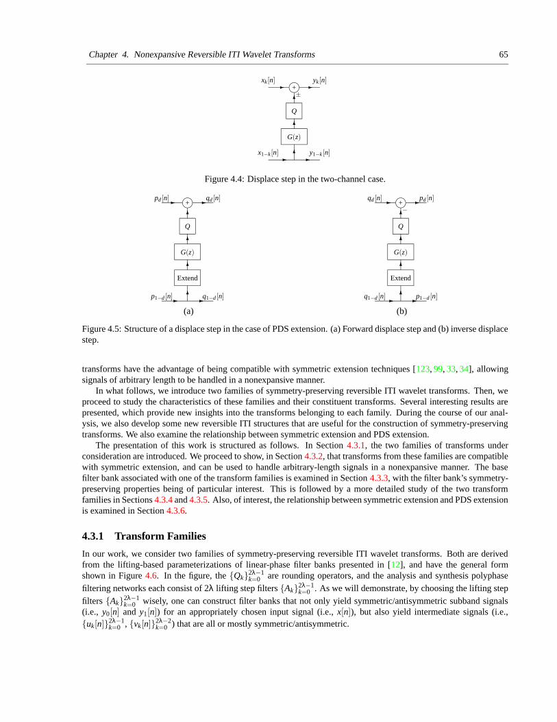
Chapter 4. Nonexpansive Reversible ITI Wavelet Transforms 65
j+
Q
G(z)
- -6
6
-
6
-±
y1−k[n]
xk[n] yk[n]
x1−k[n]
Figure 4.4: Displace step in the two-channel case.
j+
G(z)
Extend
Q
6
6
-
-
6
6-
-pd [n] qd [n]
q1−d [n]p1−d [n]
(a)
Q
j+
G(z)
Extend
6
- -
6
6
- -6
−pd [n]
p1−d [n]q1−d [n]
qd [n]
(b)
Figure 4.5: Structure of a displace step in the case of PDS extension. (a) Forward displace step and (b) inverse displacestep.
transforms have the advantage of being compatible with symmetric extension techniques [123, 99, 33, 34], allowingsignals of arbitrary length to be handled in a nonexpansive manner.
In what follows, we introduce two families of symmetry-preserving reversible ITI wavelet transforms. Then, weproceed to study the characteristics of these families and their constituent transforms. Several interesting results arepresented, which provide new insights into the transforms belonging to each family. During the course of our anal-ysis, we also develop some new reversible ITI structures that are useful for the construction of symmetry-preservingtransforms. We also examine the relationship between symmetric extension and PDS extension.
The presentation of this work is structured as follows. In Section 4.3.1, the two families of transforms underconsideration are introduced. We proceed to show, in Section 4.3.2, that transforms from these families are compatiblewith symmetric extension, and can be used to handle arbitrary-length signals in a nonexpansive manner. The basefilter bank associated with one of the transform families is examined in Section 4.3.3, with the filter bank’s symmetry-preserving properties being of particular interest. This is followed by a more detailed study of the two transformfamilies in Sections 4.3.4 and 4.3.5. Also, of interest, the relationship between symmetric extension and PDS extensionis examined in Section 4.3.6.
4.3.1 Transform Families
In our work, we consider two families of symmetry-preserving reversible ITI wavelet transforms. Both are derivedfrom the lifting-based parameterizations of linear-phase filter banks presented in [12], and have the general formshown in Figure 4.6. In the figure, the {Qk}2λ−1
k=0 are rounding operators, and the analysis and synthesis polyphase
filtering networks each consist of 2λ lifting step filters {Ak}2λ−1k=0 . As we will demonstrate, by choosing the lifting step
filters {Ak}2λ−1k=0 wisely, one can construct filter banks that not only yield symmetric/antisymmetric subband signals
(i.e., y0[n] and y1[n]) for an appropriately chosen input signal (i.e., x[n]), but also yield intermediate signals (i.e.,{uk[n]}2λ−1
k=0 , {vk[n]}2λ−2k=0 ) that are all or mostly symmetric/antisymmetric.
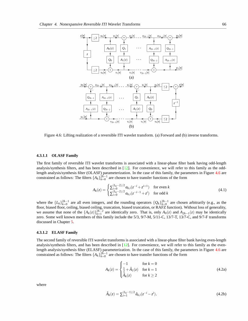
Chapter 4. Nonexpansive Reversible ITI Wavelet Transforms 66
↓2
↓2
j+
j+
z
j+
j+
A0(z)
Q0
Q1
A1(z)
6
6
6
-
??
?
?
-
-
--
?
-
- - 6
6
6
- -
-
?
?
?-
-
-
· · ·
· · ·
· · ·
· · ·
u0[n]
Q2λ−2
Q2λ−1
A2λ−1(z)
x[n] y0[n]
y1[n]
A2λ−2(z)
u1[n] u2[n] u2λ−2[n] u2λ−1[n]
v0[n] v1[n] v2[n] v2λ−2[n]
(a)
j+
j+
j+
j+
↑2
↑2
j+
z−1
A0(z)Q1
A1(z) Q0
?- - -
- 6?
-- - - -6
- -
6?
-
6
6
- --
6
?
6 6? ?Q2λ−1 A2λ−2(z)
A2λ−1(z) Q2λ−2 · · ·
· · ·
· · ·
· · ·y1[n]
y0[n] u0[n] x[n]
− −
v0[n]
− −
v1[n]v2[n]
u1[n]u2[n]u2λ−2[n]u2λ−1[n]
v2λ−2[n]
(b)
Figure 4.6: Lifting realization of a reversible ITI wavelet transform. (a) Forward and (b) inverse transforms.
4.3.1.1 OLASF Family
The first family of reversible ITI wavelet transforms is associated with a linear-phase filter bank having odd-lengthanalysis/synthesis filters, and has been described in [12]. For convenience, we will refer to this family as the odd-length analysis/synthesis filter (OLASF) parameterization. In the case of this family, the parameters in Figure 4.6 areconstrained as follows: The filters {Ak}2λ−1
k=0 are chosen to have transfer functions of the form
Ak(z) =
{
∑(Lk−2)/2i=0 ak,i(z−i + zi+1) for even k
∑(Lk−2)/2i=0 ak,i(z−i−1 + zi) for odd k
(4.1)
where the {Lk}2λ−1k=0 are all even integers, and the rounding operators {Qk}2λ−1
k=0 are chosen arbitrarily (e.g., as thefloor, biased floor, ceiling, biased ceiling, truncation, biased truncation, or RAFZ function). Without loss of generality,we assume that none of the {Ak(z)}2λ−2
k=1 are identically zero. That is, only A0(z) and A2λ−1(z) may be identicallyzero. Some well known members of this family include the 5/3, 9/7-M, 5/11-C, 13/7-T, 13/7-C, and 9/7-F transformsdiscussed in Chapter 5.
4.3.1.2 ELASF Family
The second family of reversible ITI wavelet transforms is associated with a linear-phase filter bank having even-lengthanalysis/synthesis filters, and has been described in [12]. For convenience, we will refer to this family as the even-length analysis/synthesis filter (ELASF) parameterization. In the case of this family, the parameters in Figure 4.6 areconstrained as follows: The filters {Ak}2λ−1
k=0 are chosen to have transfer functions of the form
Ak(z) =
−1 for k = 012 + A1(z) for k = 1
Ak(z) for k ≥ 2
(4.2a)
where
Ak(z) = ∑(Lk−1)/2i=1 ak,i(z−i − zi), (4.2b)
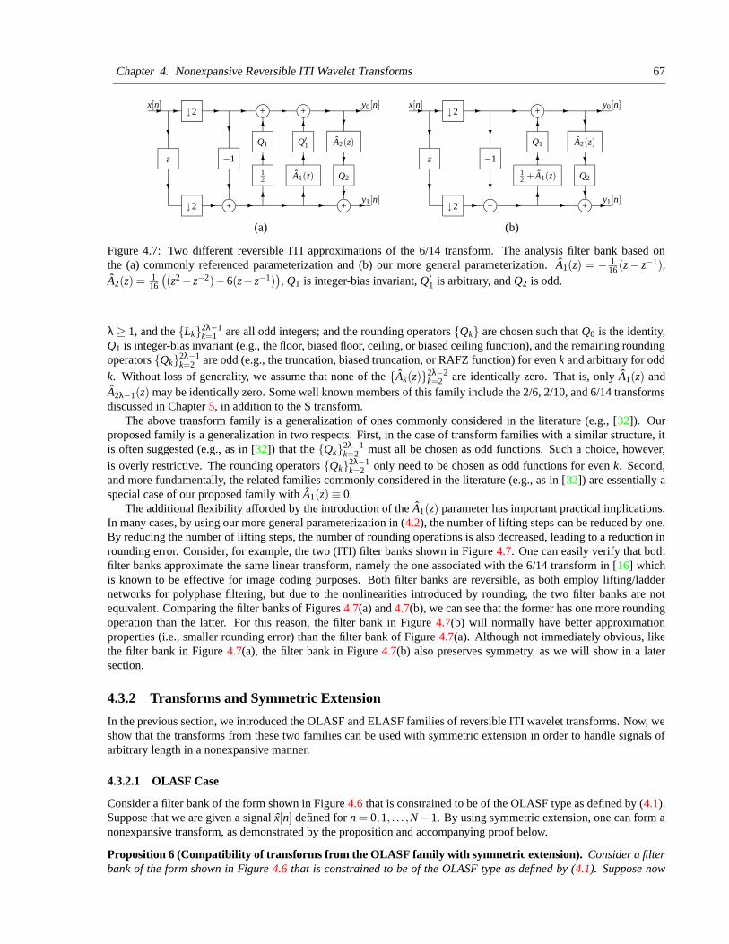
Chapter 4. Nonexpansive Reversible ITI Wavelet Transforms 67
↓2
↓2
z
j+
j+ j+
j+
−1
Q1
12
-
?
?
-
?
?-
-
6
6
6-
6
6
6
-?
?
?--
- --
-
x[n]
A1(z)
Q′1 A2(z)
Q2
y1[n]
y0[n]
(a)
↓2
↓2
z
j+
j+
j+
12 + A1(z)
−1
Q1
-
?
?
-
?
?
-
6
6
6
-
-
--?
?
?- - -
x[n]
A2(z)
y0[n]
y1[n]
Q2
(b)
Figure 4.7: Two different reversible ITI approximations of the 6/14 transform. The analysis filter bank based onthe (a) commonly referenced parameterization and (b) our more general parameterization. A1(z) = − 1
16 (z− z−1),A2(z) = 1
16
((z2 − z−2)−6(z− z−1)
), Q1 is integer-bias invariant, Q′
1 is arbitrary, and Q2 is odd.
λ ≥ 1, and the {Lk}2λ−1k=1 are all odd integers; and the rounding operators {Qk} are chosen such that Q0 is the identity,
Q1 is integer-bias invariant (e.g., the floor, biased floor, ceiling, or biased ceiling function), and the remaining roundingoperators {Qk}2λ−1
k=2 are odd (e.g., the truncation, biased truncation, or RAFZ function) for even k and arbitrary for oddk. Without loss of generality, we assume that none of the {Ak(z)}2λ−2
k=2 are identically zero. That is, only A1(z) andA2λ−1(z) may be identically zero. Some well known members of this family include the 2/6, 2/10, and 6/14 transformsdiscussed in Chapter 5, in addition to the S transform.
The above transform family is a generalization of ones commonly considered in the literature (e.g., [32]). Ourproposed family is a generalization in two respects. First, in the case of transform families with a similar structure, itis often suggested (e.g., as in [32]) that the {Qk}2λ−1
k=2 must all be chosen as odd functions. Such a choice, however,is overly restrictive. The rounding operators {Qk}2λ−1
k=2 only need to be chosen as odd functions for even k. Second,and more fundamentally, the related families commonly considered in the literature (e.g., as in [32]) are essentially aspecial case of our proposed family with A1(z) ≡ 0.
The additional flexibility afforded by the introduction of the A1(z) parameter has important practical implications.In many cases, by using our more general parameterization in (4.2), the number of lifting steps can be reduced by one.By reducing the number of lifting steps, the number of rounding operations is also decreased, leading to a reduction inrounding error. Consider, for example, the two (ITI) filter banks shown in Figure 4.7. One can easily verify that bothfilter banks approximate the same linear transform, namely the one associated with the 6/14 transform in [16] whichis known to be effective for image coding purposes. Both filter banks are reversible, as both employ lifting/laddernetworks for polyphase filtering, but due to the nonlinearities introduced by rounding, the two filter banks are notequivalent. Comparing the filter banks of Figures 4.7(a) and 4.7(b), we can see that the former has one more roundingoperation than the latter. For this reason, the filter bank in Figure 4.7(b) will normally have better approximationproperties (i.e., smaller rounding error) than the filter bank of Figure 4.7(a). Although not immediately obvious, likethe filter bank in Figure 4.7(a), the filter bank in Figure 4.7(b) also preserves symmetry, as we will show in a latersection.
4.3.2 Transforms and Symmetric Extension
In the previous section, we introduced the OLASF and ELASF families of reversible ITI wavelet transforms. Now, weshow that the transforms from these two families can be used with symmetric extension in order to handle signals ofarbitrary length in a nonexpansive manner.
4.3.2.1 OLASF Case
Consider a filter bank of the form shown in Figure 4.6 that is constrained to be of the OLASF type as defined by (4.1).Suppose that we are given a signal x[n] defined for n = 0,1, . . . ,N −1. By using symmetric extension, one can form anonexpansive transform, as demonstrated by the proposition and accompanying proof below.
Proposition 6 (Compatibility of transforms from the OLASF family with symmetric extension). Consider a filterbank of the form shown in Figure 4.6 that is constrained to be of the OLASF type as defined by (4.1). Suppose now
Chapter 4. Nonexpansive Reversible ITI Wavelet Transforms 68
that we are given a signal x[n] defined for n = 0,1, . . . ,N−1. If we choose x[n], the input to the analysis filter bank, asthe symmetric extension of x[n] given by
x[n] =x[min(mod(n−K,2N −2),2N −2−mod(n−K,2N −2))], K ∈ Z
(i.e., x[n] is defined such that x[n] = x[n+2N −2] and x[n] = x[2K −n]), then
1. y0[n] is completely characterized by its N0 samples at indices⌈
K2
⌉,⌈
K2
⌉+1, . . . ,
⌊K+N−1
2
⌋;
2. y1[n] is completely characterized by its N1 samples at indices⌈
K−12
⌉,⌈
K−12
⌉+1, . . . ,
⌊K+N−2
2
⌋; and
3. N0 +N1 = N (i.e., the transform is nonexpansive).
Proof. Consider the OLASF-type system associated with Figure 4.6. Evidently, x[n] is (2N−2)-periodic and symmet-ric about K and K +N −1 (with additional pairs of symmetry points following from periodicity). From the propertiesof downsampling, one can show that u0[n] is (N−1)-periodic and symmetric about K
2 and K+N−12 , and v0[n] is (N−1)-
periodic and symmetric about K−12 and K+N−2
2 . Consider now the first lifting step (associated with filter A0). Since,from (4.1), the filter A0 has a group delay of − 1
2 and the rounding operator Q0 preserves symmetry, the adder (follow-ing Q0) is summing two (N −1)-periodic symmetric signals with the same symmetry centers. Thus, the adder output,v1[n], is also (N − 1)-periodic and symmetric with the same symmetry centers, namely K−1
2 and K+N−22 . Consider
now the second lifting step (associated with filter A1). Since, from (4.1), the filter A1 has a group delay of 12 and the
rounding operator Q1 preserves symmetry, both adder inputs are (N − 1)-periodic symmetric signals with the samesymmetry centers. Therefore, the adder output, u2[n], must also be (N − 1)-periodic and symmetric with the samesymmetry centers, namely K
2 and K+N−12 . By repeating the above reasoning for each of the remaining lifting steps,
we have that the {uk[n]}2λ−1k=0 and y0[n] are all (N − 1)-periodic and symmetric about K
2 and K+N−12 . Likewise, the
{vk[n]}2λ−2k=0 and y1[n] are all (N −1)-periodic and symmetric about K−1
2 and K+N−22 .
By examining the form of the various signals, we can see that the {uk[n]}2λ−1k=0 and y0[n] are completely character-
ized by their samples at indices⌈
K2
⌉,⌈
K2
⌉+1, . . . ,
⌊K+N−1
2
⌋, for a total of N0 independent samples, where
N04=⌊
K+N−12
⌋−⌈
K2
⌉+1. (4.3)
Similarly, we have that the {vk[n]}2λ−2k=0 and y1[n] are completely characterized by their samples at indices
⌈K−1
2
⌉,⌈
K−12
⌉+
1, . . . ,⌊
K+N−22
⌋, for a total of N1 independent samples, where
N14=⌊
K+N−22
⌋−⌈
K−12
⌉+1. (4.4)
Using (2.11) and (2.10), we can further simplify (4.3) and (4.4) to obtain
N0 =
N2 for even NN+1
2 for odd N, even KN−1
2 for odd N, odd K,
and N1 =
N2 for even NN−1
2 for odd N, even KN+1
2 for odd N, odd K.
(4.5)
Thus, from (4.5), we have that, regardless of the parities of K and N, N0 + N1 = N. In other words, the total numberof independent samples in the transformed signal is always equal to the number of samples in the original signal, andthe resulting transform is, therefore, nonexpansive.
4.3.2.2 ELASF Case
Consider a filter bank of the form shown in Figure 4.6 that is constrained to be of the ELASF type as defined by (4.2).Suppose that we are given a signal x[n] defined for n = 0,1, . . . ,N −1. By using symmetric extension, one can form anonexpansive transform, as demonstrated by the proposition and accompanying proof below.
Proposition 7 (Compatibility of transforms from the ELASF family with symmetric extension). Consider a filterbank of the form shown in Figure 4.6 that is constrained to be of the ELASF type as defined by (4.2). Suppose now
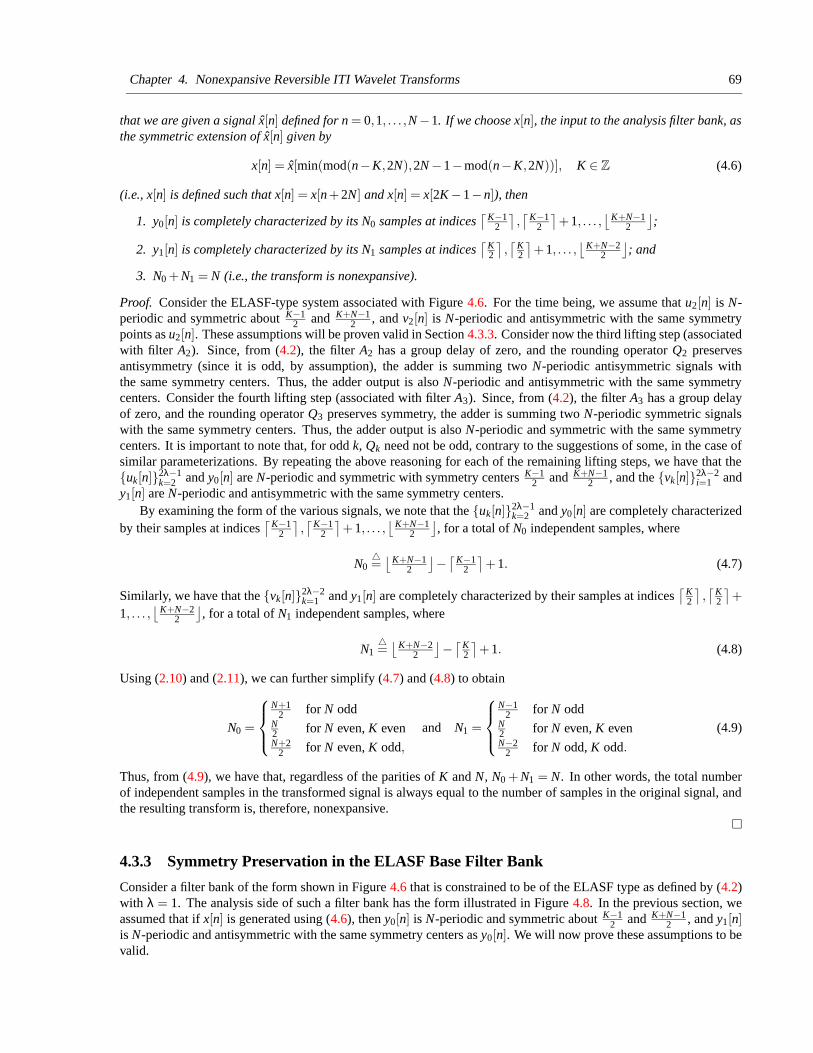
Chapter 4. Nonexpansive Reversible ITI Wavelet Transforms 69
that we are given a signal x[n] defined for n = 0,1, . . . ,N−1. If we choose x[n], the input to the analysis filter bank, asthe symmetric extension of x[n] given by
x[n] = x[min(mod(n−K,2N),2N −1−mod(n−K,2N))], K ∈ Z (4.6)
(i.e., x[n] is defined such that x[n] = x[n+2N] and x[n] = x[2K −1−n]), then
1. y0[n] is completely characterized by its N0 samples at indices⌈
K−12
⌉,⌈
K−12
⌉+1, . . . ,
⌊K+N−1
2
⌋;
2. y1[n] is completely characterized by its N1 samples at indices⌈
K2
⌉,⌈
K2
⌉+1, . . . ,
⌊K+N−2
2
⌋; and
3. N0 +N1 = N (i.e., the transform is nonexpansive).
Proof. Consider the ELASF-type system associated with Figure 4.6. For the time being, we assume that u2[n] is N-periodic and symmetric about K−1
2 and K+N−12 , and v2[n] is N-periodic and antisymmetric with the same symmetry
points as u2[n]. These assumptions will be proven valid in Section 4.3.3. Consider now the third lifting step (associatedwith filter A2). Since, from (4.2), the filter A2 has a group delay of zero, and the rounding operator Q2 preservesantisymmetry (since it is odd, by assumption), the adder is summing two N-periodic antisymmetric signals withthe same symmetry centers. Thus, the adder output is also N-periodic and antisymmetric with the same symmetrycenters. Consider the fourth lifting step (associated with filter A3). Since, from (4.2), the filter A3 has a group delayof zero, and the rounding operator Q3 preserves symmetry, the adder is summing two N-periodic symmetric signalswith the same symmetry centers. Thus, the adder output is also N-periodic and symmetric with the same symmetrycenters. It is important to note that, for odd k, Qk need not be odd, contrary to the suggestions of some, in the case ofsimilar parameterizations. By repeating the above reasoning for each of the remaining lifting steps, we have that the{uk[n]}2λ−1
k=2 and y0[n] are N-periodic and symmetric with symmetry centers K−12 and K+N−1
2 , and the {vk[n]}2λ−2i=1 and
y1[n] are N-periodic and antisymmetric with the same symmetry centers.By examining the form of the various signals, we note that the {uk[n]}2λ−1
k=2 and y0[n] are completely characterizedby their samples at indices
⌈K−1
2
⌉,⌈
K−12
⌉+1, . . . ,
⌊K+N−1
2
⌋, for a total of N0 independent samples, where
N04=⌊
K+N−12
⌋−⌈
K−12
⌉+1. (4.7)
Similarly, we have that the {vk[n]}2λ−2k=1 and y1[n] are completely characterized by their samples at indices
⌈K2
⌉,⌈
K2
⌉+
1, . . . ,⌊
K+N−22
⌋, for a total of N1 independent samples, where
N14=⌊
K+N−22
⌋−⌈
K2
⌉+1. (4.8)
Using (2.10) and (2.11), we can further simplify (4.7) and (4.8) to obtain
N0 =
N+12 for N odd
N2 for N even, K evenN+2
2 for N even, K odd,
and N1 =
N−12 for N odd
N2 for N even, K evenN−2
2 for N odd, K odd.
(4.9)
Thus, from (4.9), we have that, regardless of the parities of K and N, N0 + N1 = N. In other words, the total numberof independent samples in the transformed signal is always equal to the number of samples in the original signal, andthe resulting transform is, therefore, nonexpansive.
4.3.3 Symmetry Preservation in the ELASF Base Filter Bank
Consider a filter bank of the form shown in Figure 4.6 that is constrained to be of the ELASF type as defined by (4.2)with λ = 1. The analysis side of such a filter bank has the form illustrated in Figure 4.8. In the previous section, weassumed that if x[n] is generated using (4.6), then y0[n] is N-periodic and symmetric about K−1
2 and K+N−12 , and y1[n]
is N-periodic and antisymmetric with the same symmetry centers as y0[n]. We will now prove these assumptions to bevalid.
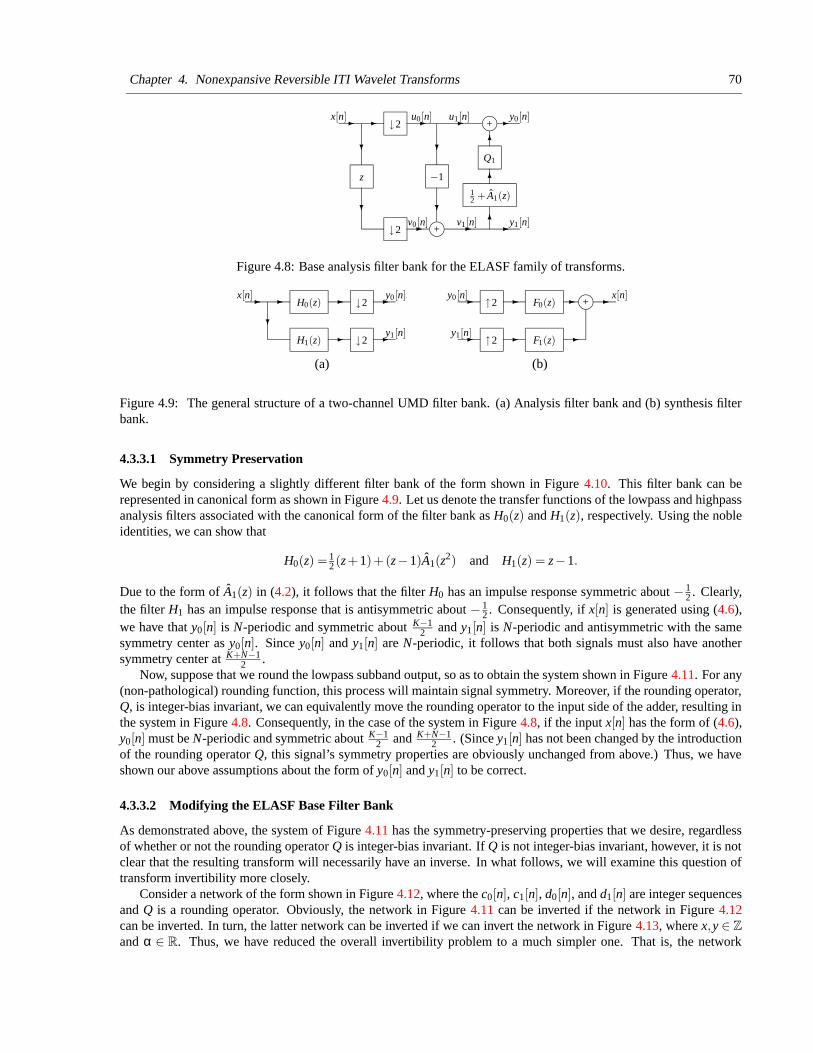
Chapter 4. Nonexpansive Reversible ITI Wavelet Transforms 70
-
- -
?
? ?
?
-
6
6
6
-
-
-
-↓2 j+
↓2
z −1
j+x[n]
12 + A1(z)
y0[n]
y1[n]
Q1
v1[n]v0[n]
u0[n] u1[n]
Figure 4.8: Base analysis filter bank for the ELASF family of transforms.
↓2
↓2
H1(z)
H0(z)- -
?
-
-
-
-
x[n] y0[n]
y1[n]
(a)
↑2 j+
↑2
F0(z)
F1(z)
-
- - -
- - -y0[n]
y1[n]
x[n]
(b)
Figure 4.9: The general structure of a two-channel UMD filter bank. (a) Analysis filter bank and (b) synthesis filterbank.
4.3.3.1 Symmetry Preservation
We begin by considering a slightly different filter bank of the form shown in Figure 4.10. This filter bank can berepresented in canonical form as shown in Figure 4.9. Let us denote the transfer functions of the lowpass and highpassanalysis filters associated with the canonical form of the filter bank as H0(z) and H1(z), respectively. Using the nobleidentities, we can show that
H0(z) = 12 (z+1)+(z−1)A1(z
2) and H1(z) = z−1.
Due to the form of A1(z) in (4.2), it follows that the filter H0 has an impulse response symmetric about − 12 . Clearly,
the filter H1 has an impulse response that is antisymmetric about − 12 . Consequently, if x[n] is generated using (4.6),
we have that y0[n] is N-periodic and symmetric about K−12 and y1[n] is N-periodic and antisymmetric with the same
symmetry center as y0[n]. Since y0[n] and y1[n] are N-periodic, it follows that both signals must also have anothersymmetry center at K+N−1
2 .Now, suppose that we round the lowpass subband output, so as to obtain the system shown in Figure 4.11. For any
(non-pathological) rounding function, this process will maintain signal symmetry. Moreover, if the rounding operator,Q, is integer-bias invariant, we can equivalently move the rounding operator to the input side of the adder, resulting inthe system in Figure 4.8. Consequently, in the case of the system in Figure 4.8, if the input x[n] has the form of (4.6),y0[n] must be N-periodic and symmetric about K−1
2 and K+N−12 . (Since y1[n] has not been changed by the introduction
of the rounding operator Q, this signal’s symmetry properties are obviously unchanged from above.) Thus, we haveshown our above assumptions about the form of y0[n] and y1[n] to be correct.
4.3.3.2 Modifying the ELASF Base Filter Bank
As demonstrated above, the system of Figure 4.11 has the symmetry-preserving properties that we desire, regardlessof whether or not the rounding operator Q is integer-bias invariant. If Q is not integer-bias invariant, however, it is notclear that the resulting transform will necessarily have an inverse. In what follows, we will examine this question oftransform invertibility more closely.
Consider a network of the form shown in Figure 4.12, where the c0[n], c1[n], d0[n], and d1[n] are integer sequencesand Q is a rounding operator. Obviously, the network in Figure 4.11 can be inverted if the network in Figure 4.12can be inverted. In turn, the latter network can be inverted if we can invert the network in Figure 4.13, where x,y ∈ Z
and α ∈ R. Thus, we have reduced the overall invertibility problem to a much simpler one. That is, the network
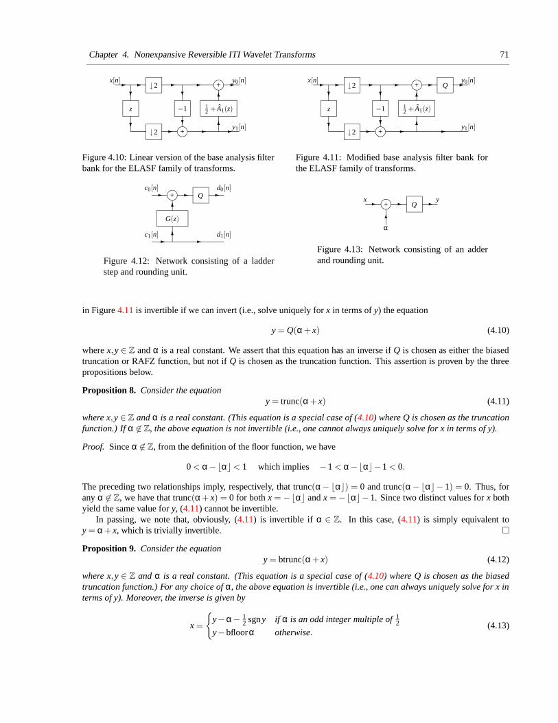
Chapter 4. Nonexpansive Reversible ITI Wavelet Transforms 71
-
?
?
- -?
? 6
6
-- -
- -
z
↓2
↓2
j+
−1
j+x[n]
12 + A1(z)
y0[n]
y1[n]
Figure 4.10: Linear version of the base analysis filterbank for the ELASF family of transforms.
-
?
?
- -?
? 6
-
6
-- -
- -
z
↓2
↓2
j+
−1
j+ Qx[n]
12 + A1(z)
y0[n]
y1[n]
Figure 4.11: Modified base analysis filter bank forthe ELASF family of transforms.
j+ Q
6
6
-
- -
-
-
G(z)
c0[n]
c1[n]
d0[n]
d1[n]
Figure 4.12: Network consisting of a ladderstep and rounding unit.
j+ Q- -
6
-x y
α
Figure 4.13: Network consisting of an adderand rounding unit.
in Figure 4.11 is invertible if we can invert (i.e., solve uniquely for x in terms of y) the equation
y = Q(α+ x) (4.10)
where x,y ∈ Z and α is a real constant. We assert that this equation has an inverse if Q is chosen as either the biasedtruncation or RAFZ function, but not if Q is chosen as the truncation function. This assertion is proven by the threepropositions below.
Proposition 8. Consider the equationy = trunc(α+ x) (4.11)
where x,y ∈ Z and α is a real constant. (This equation is a special case of (4.10) where Q is chosen as the truncationfunction.) If α 6∈ Z, the above equation is not invertible (i.e., one cannot always uniquely solve for x in terms of y).
Proof. Since α 6∈ Z, from the definition of the floor function, we have
0 < α−bαc < 1 which implies −1 < α−bαc−1 < 0.
The preceding two relationships imply, respectively, that trunc(α− bαc) = 0 and trunc(α−bαc− 1) = 0. Thus, forany α 6∈ Z, we have that trunc(α+ x) = 0 for both x = −bαc and x = −bαc−1. Since two distinct values for x bothyield the same value for y, (4.11) cannot be invertible.
In passing, we note that, obviously, (4.11) is invertible if α ∈ Z. In this case, (4.11) is simply equivalent toy = α+ x, which is trivially invertible.
Proposition 9. Consider the equationy = btrunc(α+ x) (4.12)
where x,y ∈ Z and α is a real constant. (This equation is a special case of (4.10) where Q is chosen as the biasedtruncation function.) For any choice of α, the above equation is invertible (i.e., one can always uniquely solve for x interms of y). Moreover, the inverse is given by
x =
{
y−α− 12 sgny if α is an odd integer multiple of 1
2
y−bfloorα otherwise.(4.13)
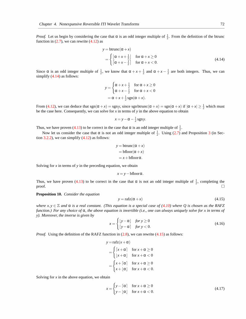
Chapter 4. Nonexpansive Reversible ITI Wavelet Transforms 72
Proof. Let us begin by considering the case that α is an odd integer multiple of 12 . From the definition of the btrunc
function in (2.7), we can rewrite (4.12) as
y = btrunc(α+ x)
=
{⌊α+ x+ 1
2
⌋for α+ x ≥ 0
⌈α+ x− 1
2
⌉for α+ x < 0.
(4.14)
Since α is an odd integer multiple of 12 , we know that α + x + 1
2 and α + x− 12 are both integers. Thus, we can
simplify (4.14) as follows:
y =
{
α+ x+ 12 for α+ x ≥ 0
α+ x− 12 for α+ x < 0
= α+ x+ 12 sgn(α+ x).
From (4.12), we can deduce that sgn(α + x) = sgny, since sgnbtrunc(α + x) = sgn(α + x) if |α+ x| ≥ 12 which must
be the case here. Consequently, we can solve for x in terms of y in the above equation to obtain
x = y−α− 12 sgny.
Thus, we have proven (4.13) to be correct in the case that α is an odd integer multiple of 12 .
Now let us consider the case that α is not an odd integer multiple of 12 . Using (2.7) and Proposition 3 (in Sec-
tion 3.2.2), we can simplify (4.12) as follows:
y = btrunc(α+ x)
= bfloor(α+ x)
= x+bfloorα.
Solving for x in terms of y in the preceding equation, we obtain
x = y−bfloorα.
Thus, we have proven (4.13) to be correct in the case that α is not an odd integer multiple of 12 , completing the
proof.
Proposition 10. Consider the equationy = rafz(α+ x) (4.15)
where x,y ∈ Z and α is a real constant. (This equation is a special case of (4.10) where Q is chosen as the RAFZfunction.) For any choice of α, the above equation is invertible (i.e., one can always uniquely solve for x in terms ofy). Moreover, the inverse is given by
x =
{
by−αc for y ≥ 0
dy−αe for y < 0.(4.16)
Proof. Using the definition of the RAFZ function in (2.8), we can rewrite (4.15) as follows:
y = rafz(x+α)
=
{
dx+αe for x+α ≥ 0
bx+αc for x+α < 0
=
{
x+ dαe for x+α ≥ 0
x+ bαc for x+α < 0.
Solving for x in the above equation, we obtain
x =
{
y−dαe for x+α ≥ 0
y−bαc for x+α < 0.(4.17)
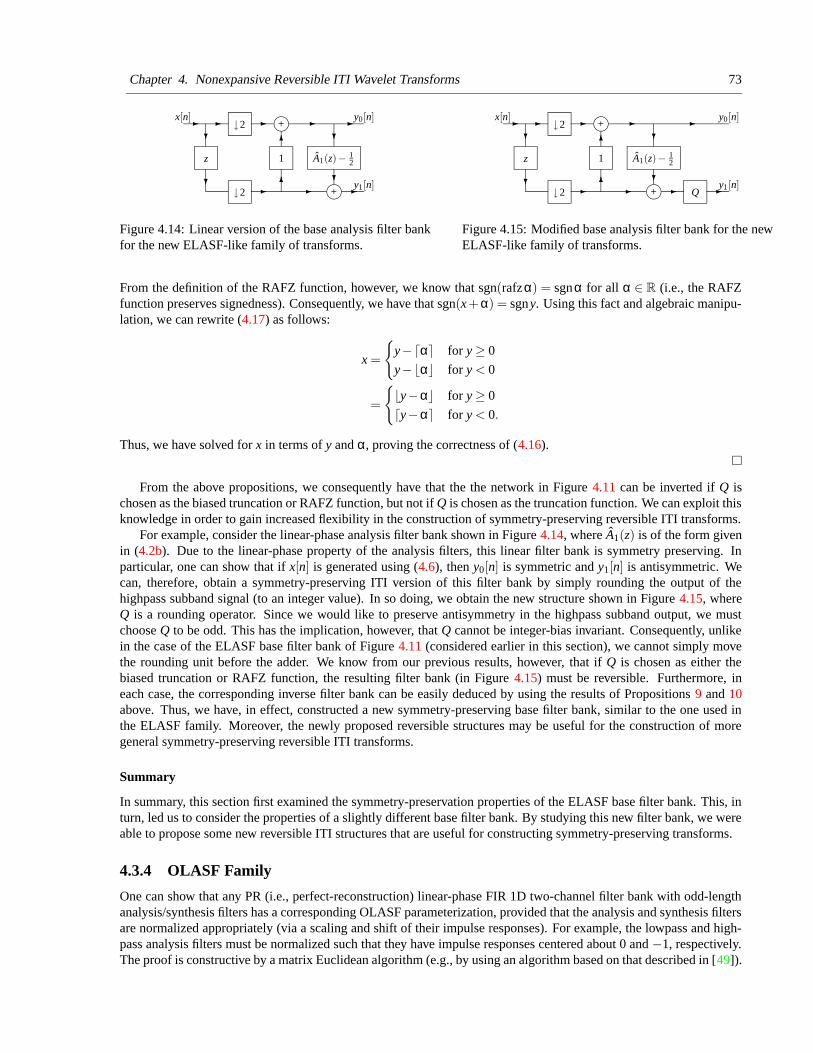
Chapter 4. Nonexpansive Reversible ITI Wavelet Transforms 73
- -?
?
-
6
6
?
?
- - -
--
z
↓2
↓2 j+
1
j+
x[n]
A1(z)− 12
y1[n]
y0[n]
Figure 4.14: Linear version of the base analysis filter bankfor the new ELASF-like family of transforms.
- -?
?
-
6
6
?
?
- - - -
- -
z
↓2
↓2 j+
1
j+ Q
x[n]
A1(z)− 12
y1[n]
y0[n]
Figure 4.15: Modified base analysis filter bank for the newELASF-like family of transforms.
From the definition of the RAFZ function, however, we know that sgn(rafzα) = sgnα for all α ∈ R (i.e., the RAFZfunction preserves signedness). Consequently, we have that sgn(x+α) = sgny. Using this fact and algebraic manipu-lation, we can rewrite (4.17) as follows:
x =
{
y−dαe for y ≥ 0
y−bαc for y < 0
=
{
by−αc for y ≥ 0
dy−αe for y < 0.
Thus, we have solved for x in terms of y and α, proving the correctness of (4.16).
From the above propositions, we consequently have that the the network in Figure 4.11 can be inverted if Q ischosen as the biased truncation or RAFZ function, but not if Q is chosen as the truncation function. We can exploit thisknowledge in order to gain increased flexibility in the construction of symmetry-preserving reversible ITI transforms.
For example, consider the linear-phase analysis filter bank shown in Figure 4.14, where A1(z) is of the form givenin (4.2b). Due to the linear-phase property of the analysis filters, this linear filter bank is symmetry preserving. Inparticular, one can show that if x[n] is generated using (4.6), then y0[n] is symmetric and y1[n] is antisymmetric. Wecan, therefore, obtain a symmetry-preserving ITI version of this filter bank by simply rounding the output of thehighpass subband signal (to an integer value). In so doing, we obtain the new structure shown in Figure 4.15, whereQ is a rounding operator. Since we would like to preserve antisymmetry in the highpass subband output, we mustchoose Q to be odd. This has the implication, however, that Q cannot be integer-bias invariant. Consequently, unlikein the case of the ELASF base filter bank of Figure 4.11 (considered earlier in this section), we cannot simply movethe rounding unit before the adder. We know from our previous results, however, that if Q is chosen as either thebiased truncation or RAFZ function, the resulting filter bank (in Figure 4.15) must be reversible. Furthermore, ineach case, the corresponding inverse filter bank can be easily deduced by using the results of Propositions 9 and 10above. Thus, we have, in effect, constructed a new symmetry-preserving base filter bank, similar to the one used inthe ELASF family. Moreover, the newly proposed reversible structures may be useful for the construction of moregeneral symmetry-preserving reversible ITI transforms.
Summary
In summary, this section first examined the symmetry-preservation properties of the ELASF base filter bank. This, inturn, led us to consider the properties of a slightly different base filter bank. By studying this new filter bank, we wereable to propose some new reversible ITI structures that are useful for constructing symmetry-preserving transforms.
4.3.4 OLASF Family
One can show that any PR (i.e., perfect-reconstruction) linear-phase FIR 1D two-channel filter bank with odd-lengthanalysis/synthesis filters has a corresponding OLASF parameterization, provided that the analysis and synthesis filtersare normalized appropriately (via a scaling and shift of their impulse responses). For example, the lowpass and high-pass analysis filters must be normalized such that they have impulse responses centered about 0 and −1, respectively.The proof is constructive by a matrix Euclidean algorithm (e.g., by using an algorithm based on that described in [49]).
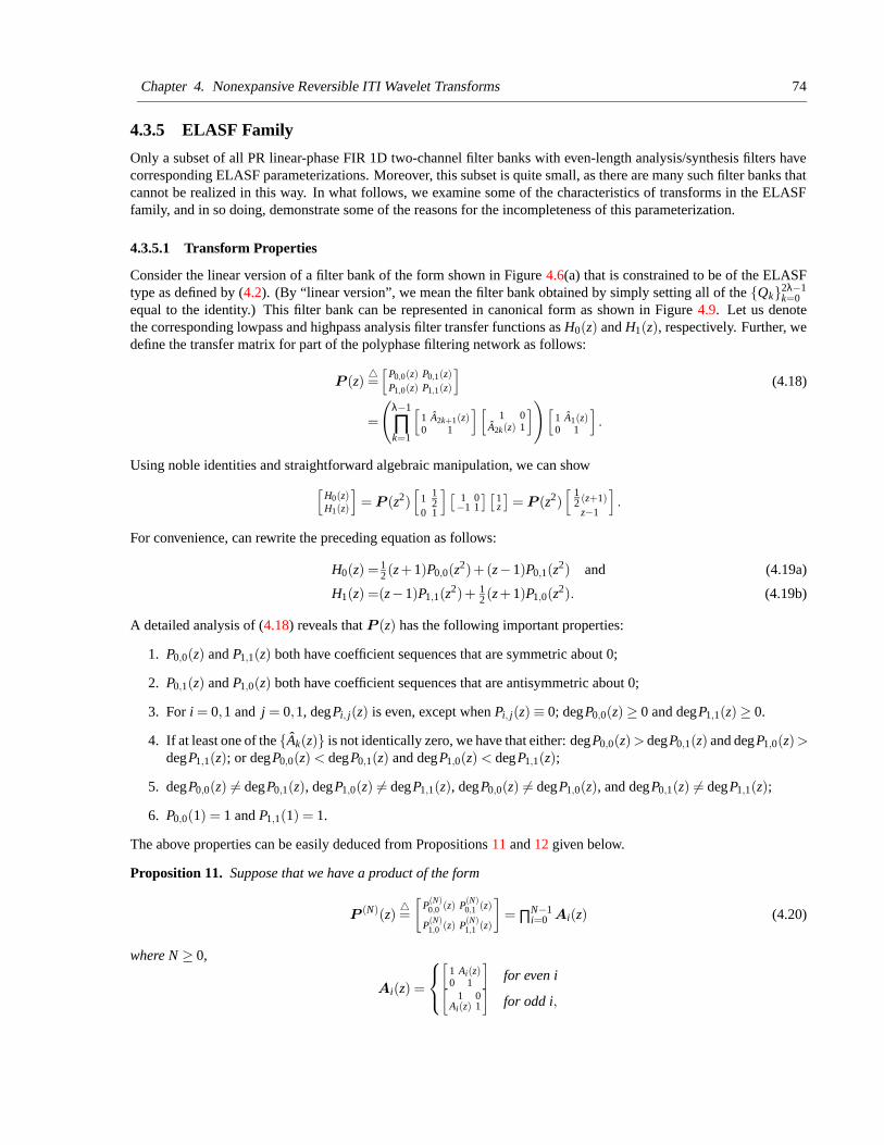
Chapter 4. Nonexpansive Reversible ITI Wavelet Transforms 74
4.3.5 ELASF Family
Only a subset of all PR linear-phase FIR 1D two-channel filter banks with even-length analysis/synthesis filters havecorresponding ELASF parameterizations. Moreover, this subset is quite small, as there are many such filter banks thatcannot be realized in this way. In what follows, we examine some of the characteristics of transforms in the ELASFfamily, and in so doing, demonstrate some of the reasons for the incompleteness of this parameterization.
4.3.5.1 Transform Properties
Consider the linear version of a filter bank of the form shown in Figure 4.6(a) that is constrained to be of the ELASFtype as defined by (4.2). (By “linear version”, we mean the filter bank obtained by simply setting all of the {Qk}2λ−1
k=0equal to the identity.) This filter bank can be represented in canonical form as shown in Figure 4.9. Let us denotethe corresponding lowpass and highpass analysis filter transfer functions as H0(z) and H1(z), respectively. Further, wedefine the transfer matrix for part of the polyphase filtering network as follows:
P (z)4=[
P0,0(z) P0,1(z)P1,0(z) P1,1(z)
]
(4.18)
=
(λ−1
∏k=1
[1 A2k+1(z)0 1
][1 0
A2k(z) 1
])[
1 A1(z)0 1
]
.
Using noble identities and straightforward algebraic manipulation, we can show
[H0(z)H1(z)
]
= P (z2)[
1 12
0 1
][1 0−1 1
][1z
]= P (z2)
[ 12 (z+1)
z−1
]
.
For convenience, can rewrite the preceding equation as follows:
H0(z) = 12 (z+1)P0,0(z
2)+(z−1)P0,1(z2) and (4.19a)
H1(z) =(z−1)P1,1(z2)+ 1
2 (z+1)P1,0(z2). (4.19b)
A detailed analysis of (4.18) reveals that P (z) has the following important properties:
1. P0,0(z) and P1,1(z) both have coefficient sequences that are symmetric about 0;
2. P0,1(z) and P1,0(z) both have coefficient sequences that are antisymmetric about 0;
3. For i = 0,1 and j = 0,1, degPi, j(z) is even, except when Pi, j(z) ≡ 0; degP0,0(z) ≥ 0 and degP1,1(z) ≥ 0.
4. If at least one of the {Ak(z)} is not identically zero, we have that either: degP0,0(z)> degP0,1(z) and degP1,0(z)>degP1,1(z); or degP0,0(z) < degP0,1(z) and degP1,0(z) < degP1,1(z);
5. degP0,0(z) 6= degP0,1(z), degP1,0(z) 6= degP1,1(z), degP0,0(z) 6= degP1,0(z), and degP0,1(z) 6= degP1,1(z);
6. P0,0(1) = 1 and P1,1(1) = 1.
The above properties can be easily deduced from Propositions 11 and 12 given below.
Proposition 11. Suppose that we have a product of the form
P (N)(z)4=
[P
(N)0,0 (z) P
(N)0,1 (z)
P(N)1,0 (z) P
(N)1,1 (z)
]
= ∏N−1i=0 Ai(z) (4.20)
where N ≥ 0,
Ai(z) =
[1 Ai(z)0 1
]
for even i[
1 0Ai(z) 1
]
for odd i,
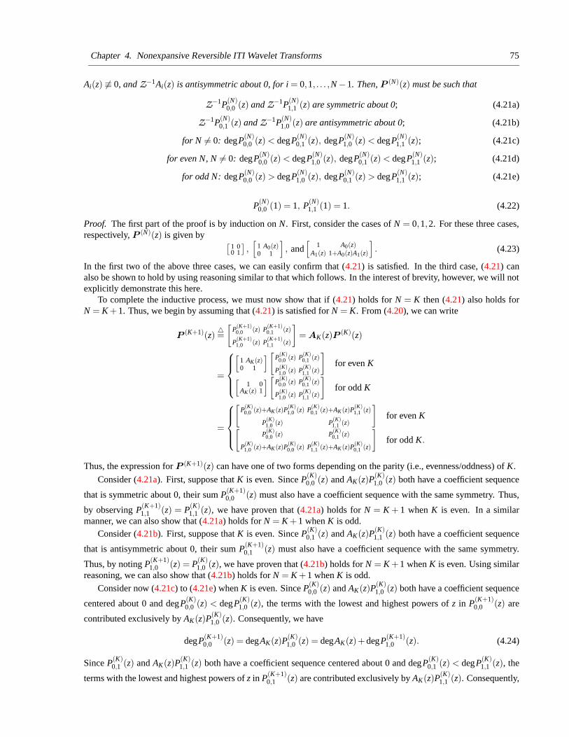
Chapter 4. Nonexpansive Reversible ITI Wavelet Transforms 75
Ai(z) 6≡ 0, and Z−1Ai(z) is antisymmetric about 0, for i = 0,1, . . . ,N −1. Then, P (N)(z) must be such that
Z−1P(N)0,0 (z) and Z−1P(N)
1,1 (z) are symmetric about 0; (4.21a)
Z−1P(N)0,1 (z) and Z−1P(N)
1,0 (z) are antisymmetric about 0; (4.21b)
for N 6= 0: degP(N)0,0 (z) < degP(N)
0,1 (z), degP(N)1,0 (z) < degP(N)
1,1 (z); (4.21c)
for even N, N 6= 0: degP(N)0,0 (z) < degP(N)
1,0 (z), degP(N)0,1 (z) < degP(N)
1,1 (z); (4.21d)
for odd N: degP(N)0,0 (z) > degP(N)
1,0 (z), degP(N)0,1 (z) > degP(N)
1,1 (z); (4.21e)
P(N)0,0 (1) = 1, P(N)
1,1 (1) = 1. (4.22)
Proof. The first part of the proof is by induction on N. First, consider the cases of N = 0,1,2. For these three cases,respectively, P (N)(z) is given by
[1 00 1
],[
1 A0(z)0 1
]
, and[
1 A0(z)A1(z) 1+A0(z)A1(z)
]
. (4.23)
In the first two of the above three cases, we can easily confirm that (4.21) is satisfied. In the third case, (4.21) canalso be shown to hold by using reasoning similar to that which follows. In the interest of brevity, however, we will notexplicitly demonstrate this here.
To complete the inductive process, we must now show that if (4.21) holds for N = K then (4.21) also holds forN = K +1. Thus, we begin by assuming that (4.21) is satisfied for N = K. From (4.20), we can write
P (K+1)(z)4=
[P
(K+1)0,0 (z) P
(K+1)0,1 (z)
P(K+1)1,0 (z) P
(K+1)1,1 (z)
]
= AK(z)P (K)(z)
=
[1 AK(z)0 1
][P
(K)0,0 (z) P
(K)0,1 (z)
P(K)1,0 (z) P
(K)1,1 (z)
]
for even K
[1 0
AK(z) 1
][P
(K)0,0 (z) P
(K)0,1 (z)
P(K)1,0 (z) P
(K)1,1 (z)
]
for odd K
=
[P
(K)0,0 (z)+AK(z)P
(K)1,0 (z) P
(K)0,1 (z)+AK(z)P
(K)1,1 (z)
P(K)1,0 (z) P
(K)1,1 (z)
]
for even K[
P(K)0,0 (z) P
(K)0,1 (z)
P(K)1,0 (z)+AK(z)P
(K)0,0 (z) P
(K)1,1 (z)+AK(z)P
(K)0,1 (z)
]
for odd K.
Thus, the expression for P (K+1)(z) can have one of two forms depending on the parity (i.e., evenness/oddness) of K.
Consider (4.21a). First, suppose that K is even. Since P(K)0,0 (z) and AK(z)P(K)
1,0 (z) both have a coefficient sequence
that is symmetric about 0, their sum P(K+1)0,0 (z) must also have a coefficient sequence with the same symmetry. Thus,
by observing P(K+1)1,1 (z) = P(K)
1,1 (z), we have proven that (4.21a) holds for N = K + 1 when K is even. In a similarmanner, we can also show that (4.21a) holds for N = K +1 when K is odd.
Consider (4.21b). First, suppose that K is even. Since P(K)0,1 (z) and AK(z)P(K)
1,1 (z) both have a coefficient sequence
that is antisymmetric about 0, their sum P(K+1)0,1 (z) must also have a coefficient sequence with the same symmetry.
Thus, by noting P(K+1)1,0 (z) = P(K)
1,0 (z), we have proven that (4.21b) holds for N = K +1 when K is even. Using similarreasoning, we can also show that (4.21b) holds for N = K +1 when K is odd.
Consider now (4.21c) to (4.21e) when K is even. Since P(K)0,0 (z) and AK(z)P(K)
1,0 (z) both have a coefficient sequence
centered about 0 and degP(K)0,0 (z) < degP(K)
1,0 (z), the terms with the lowest and highest powers of z in P(K+1)0,0 (z) are
contributed exclusively by AK(z)P(K)1,0 (z). Consequently, we have
degP(K+1)0,0 (z) = degAK(z)P(K)
1,0 (z) = degAK(z)+degP(K+1)1,0 (z). (4.24)
Since P(K)0,1 (z) and AK(z)P(K)
1,1 (z) both have a coefficient sequence centered about 0 and degP(K)0,1 (z) < degP(K)
1,1 (z), the
terms with the lowest and highest powers of z in P(K+1)0,1 (z) are contributed exclusively by AK(z)P(K)
1,1 (z). Consequently,
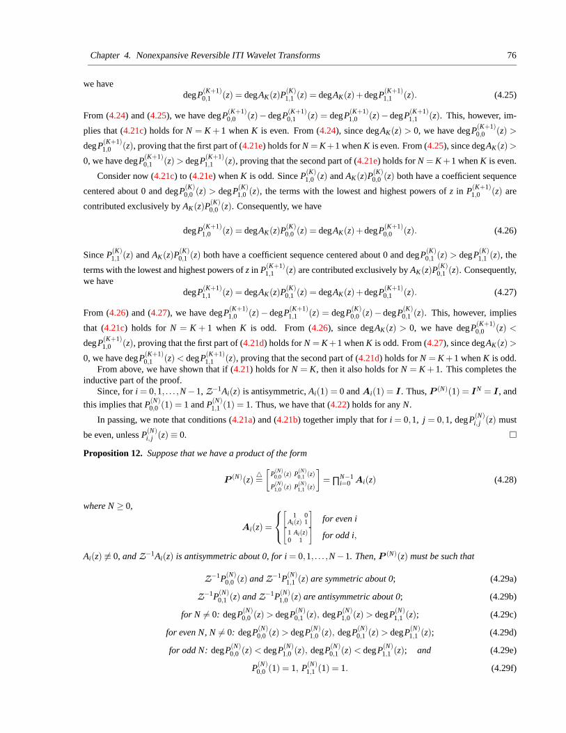
Chapter 4. Nonexpansive Reversible ITI Wavelet Transforms 76
we havedegP(K+1)
0,1 (z) = degAK(z)P(K)1,1 (z) = degAK(z)+degP(K+1)
1,1 (z). (4.25)
From (4.24) and (4.25), we have degP(K+1)0,0 (z)− degP(K+1)
0,1 (z) = degP(K+1)1,0 (z)− degP(K+1)
1,1 (z). This, however, im-
plies that (4.21c) holds for N = K + 1 when K is even. From (4.24), since degAK(z) > 0, we have degP(K+1)0,0 (z) >
degP(K+1)1,0 (z), proving that the first part of (4.21e) holds for N = K +1 when K is even. From (4.25), since degAK(z) >
0, we have degP(K+1)0,1 (z) > degP(K+1)
1,1 (z), proving that the second part of (4.21e) holds for N = K +1 when K is even.
Consider now (4.21c) to (4.21e) when K is odd. Since P(K)1,0 (z) and AK(z)P(K)
0,0 (z) both have a coefficient sequence
centered about 0 and degP(K)0,0 (z) > degP(K)
1,0 (z), the terms with the lowest and highest powers of z in P(K+1)1,0 (z) are
contributed exclusively by AK(z)P(K)0,0 (z). Consequently, we have
degP(K+1)1,0 (z) = degAK(z)P(K)
0,0 (z) = degAK(z)+degP(K+1)0,0 (z). (4.26)
Since P(K)1,1 (z) and AK(z)P(K)
0,1 (z) both have a coefficient sequence centered about 0 and degP(K)0,1 (z) > degP(K)
1,1 (z), the
terms with the lowest and highest powers of z in P(K+1)1,1 (z) are contributed exclusively by AK(z)P(K)
0,1 (z). Consequently,we have
degP(K+1)1,1 (z) = degAK(z)P(K)
0,1 (z) = degAK(z)+degP(K+1)0,1 (z). (4.27)
From (4.26) and (4.27), we have degP(K+1)1,0 (z)− degP(K+1)
1,1 (z) = degP(K)0,0 (z)− degP(K)
0,1 (z). This, however, implies
that (4.21c) holds for N = K + 1 when K is odd. From (4.26), since degAK(z) > 0, we have degP(K+1)0,0 (z) <
degP(K+1)1,0 (z), proving that the first part of (4.21d) holds for N = K +1 when K is odd. From (4.27), since degAK(z) >
0, we have degP(K+1)0,1 (z) < degP(K+1)
1,1 (z), proving that the second part of (4.21d) holds for N = K +1 when K is odd.From above, we have shown that if (4.21) holds for N = K, then it also holds for N = K + 1. This completes the
inductive part of the proof.Since, for i = 0,1, . . . ,N −1, Z−1Ai(z) is antisymmetric, Ai(1) = 0 and Ai(1) = I . Thus, P (N)(1) = IN = I , and
this implies that P(N)0,0 (1) = 1 and P(N)
1,1 (1) = 1. Thus, we have that (4.22) holds for any N.
In passing, we note that conditions (4.21a) and (4.21b) together imply that for i = 0,1, j = 0,1, degP(N)i, j (z) must
be even, unless P(N)i, j (z) ≡ 0.
Proposition 12. Suppose that we have a product of the form
P (N)(z)4=
[P
(N)0,0 (z) P
(N)0,1 (z)
P(N)1,0 (z) P
(N)1,1 (z)
]
= ∏N−1i=0 Ai(z) (4.28)
where N ≥ 0,
Ai(z) =
[1 0
Ai(z) 1
]
for even i[
1 Ai(z)0 1
]
for odd i,
Ai(z) 6≡ 0, and Z−1Ai(z) is antisymmetric about 0, for i = 0,1, . . . ,N −1. Then, P (N)(z) must be such that
Z−1P(N)0,0 (z) and Z−1P(N)
1,1 (z) are symmetric about 0; (4.29a)
Z−1P(N)0,1 (z) and Z−1P(N)
1,0 (z) are antisymmetric about 0; (4.29b)
for N 6= 0: degP(N)0,0 (z) > degP(N)
0,1 (z), degP(N)1,0 (z) > degP(N)
1,1 (z); (4.29c)
for even N, N 6= 0: degP(N)0,0 (z) > degP(N)
1,0 (z), degP(N)0,1 (z) > degP(N)
1,1 (z); (4.29d)
for odd N: degP(N)0,0 (z) < degP(N)
1,0 (z), degP(N)0,1 (z) < degP(N)
1,1 (z); and (4.29e)
P(N)0,0 (1) = 1, P(N)
1,1 (1) = 1. (4.29f)
Chapter 4. Nonexpansive Reversible ITI Wavelet Transforms 77
Proof. We begin by rewriting (4.28) as
P (N)(z) = J(
∏N−1i=0 Ai(z)
)J (4.30)
where
Ai(z) =
[1 Ai(z)0 1
]
for even i[
1 0Ai(z) 1
]
for odd i.
From (4.30), we can write
P (z)4=[
P0,0(z) P0,1(z)
P1,0(z) P1,1(z)
]
= ∏N−1i=0 Ai(z) (4.31)
whereP (z) = JP (N)(z)J . (4.32)
From (4.32), we have that P (z) and P (N)(z) are related as follows:
P(N)0,0 (z) = P1,1(z), P(N)
0,1 (z) = P1,0(z), (4.33)
P(N)1,0 (z) = P0,1(z), and P(N)
1,1 (z) = P0,0(z).
We now observe that the product in (4.31) is of the same form considered in Proposition 11. Consequently, we caneasily show, by using Proposition 11 and (4.33), that (4.29) holds.
In what follows, the above properties will be used to study various characteristics of the analysis filters such as theform of their transfer functions, their lengths, and their DC and Nyquist gains. These characteristics will also be usedto explain the reasons for the incompleteness of the ELASF parameterization.
4.3.5.2 Lowpass Analysis Filter Transfer Function
For convenience, let us denote the first and second terms in the expression for H0(z) in (4.19a) as B(z) and C(z),
respectively. That is, we define B(z)4= 1
2 (z+1)P0,0(z2) and C(z)4= (z−1)P0,1(z2). Due to the form of P0,0(z2) (which
is implied by property 1 of P (z)), B(z) has a coefficient sequence b[n] that is symmetric about − 12 with adjacent pairs
of samples being equal in value (i.e., b[2n] = b[2n− 1]). Likewise, due to the form of P0,1(z2) (which is implied byproperty 2 of P (z)), C(z) has a coefficient sequence c[n] that is symmetric about − 1
2 with adjacent pairs of samplesbeing equal in magnitude but opposite in sign (i.e., c[2n] = −c[2n− 1]). Suppose that P0,1(z) 6≡ 0. In this case, fromproperties 3 and 5 of P (z), we know that degP0,0(z2) and degP0,1(z2) must differ by a nonzero integer multiple of 4.Since H0(z) = B(z)+C(z), H0(z) must have a coefficient sequence that is symmetric about − 1
2 and begins and endswith pairs of coefficients that are either equal or equal in magnitude but opposite in sign. In the degenerate case, inwhich P0,1(z) ≡ 0, we simply have H0(z) = 1
2 (z + 1). By considering the degrees of B(z) and C(z), we can also seethat
degH0(z) = 1+2max(degP0,0(z),degP0,1(z)). (4.34)
Since, by property 3 of P (z), degP0,0(z) is always even and degP0,1(z) is even (except when P0,1(z)≡ 0), we have thatdegH0(z) is odd. Thus, as had been suggested earlier, H0 is an even-length filter.
4.3.5.3 Highpass Analysis Filter Transfer Function
For convenience, let us denote the first and second terms in the expression for H1(z) in (4.19b) as B(z) and C(z),
respectively. That is, we define B(z)4= (z−1)P1,1(z2) and C(z)
4= 1
2 (z+1)P1,0(z2). Due to the form of P1,1(z2) (whichis implied by property 1 of P (z)), B(z) has a coefficient sequence b[n] that is antisymmetric about − 1
2 with adjacentpairs of samples being equal in magnitude but opposite in sign (i.e., b[2n] = −b[2n− 1]). Likewise, due to the formof P1,0(z2) (which is implied by property 2 of P (z)), C(z) has a coefficient sequence c[n] that is antisymmetric about− 1
2 with adjacent pairs of samples being equal (i.e., c[2n] = c[2n− 1]). Suppose that P1,0(z) 6≡ 0. In this case, fromproperties 3 and 5 of P (z), we know that degP1,1(z2) and degP1,0(z2) must differ by a nonzero integer multiple of4. Since H1(z) = B(z)+C(z), H1(z) must have a coefficient sequence that is antisymmetric about − 1
2 and begins and
Chapter 4. Nonexpansive Reversible ITI Wavelet Transforms 78
ends with pairs of coefficients that are either equal or equal in magnitude but opposite in sign. In the degenerate case,in which P1,0(z) ≡ 0, we simply have H1(z) = z−1. By examining the degrees of B(z) and C(z), we can see that
degH1(z) = 1+2max(degP1,1(z),degP1,0(z)). (4.35)
Since, by property 3 of P (z), degP1,1(z) is always even and degP1,0(z) is even (except when P1,0(z)≡ 0), we have thatdegH1(z) is odd. Thus, as had been suggested earlier, H1 is an even-length filter.
4.3.5.4 Analysis Filter Lengths
The above results are significant as they show that H0(z) and H1(z) both have a highly structured form (i.e., theircoefficient sequences are each the sum of two highly structured sequences). Examining the expression for degH0(z)and degH1(z), we can make one further observation regarding the analysis filters. That is, except in the degeneratecase in which all of the {Ak(z)}2λ−1
k=1 are identically zero, the analysis filters cannot have the same length. To see whythis is so, we proceed as below.
Since, by assumption, at least one of the {Ak(z)}2λ−1k=1 is not identically zero, property 4 of P (z) implies that
two cases are possible: 1) degP0,0(z) > degP0,1(z) and degP1,0(z) > degP1,1(z); or 2) degP0,0(z) < degP0,1(z) anddegP1,0(z) < degP1,1(z). In the first case, we have from (4.34) and (4.35) that degH0(z) = 1 + 2degP0,0(z) anddegH1(z) = 1 + 2degP1,0(z). From property 5 of P(z), however, we know that degP0,0(z) 6= degP1,0(z). Therefore,degH0(z) 6= degH1(z). In the second case, we have from (4.34) and (4.35) that degH0(z) = 1 + 2degP0,1(z) anddegH1(z) = 1 + 2degP1,1(z). From property 5 of P (z), however, we know that degP0,1(z) 6= degP1,1(z). Therefore,degH0(z) 6= degH1(z). By combining the results for the above two cases, we have that degH0(z) 6= degH1(z), exceptin the degenerate case in which all of the {Ak(z)}2λ−1
k=1 are identically zero. Consequently, the analysis filters cannothave the same lengths, except in this degenerate case.
4.3.5.5 Incompleteness of Parameterization
In order to belong to the ELASF family, a transform must have analysis filters of the form described above. Obviously,the close relationship between pairs of samples in the analysis filter impulse responses is quite constraining. For thisreason, the ELASF family cannot be a complete parameterization of all PR linear-phase FIR 1D two-channel filterbanks with even-length filters. Furthermore, an even more basic reason exists for this lack of completeness. As notedabove, the analysis filters cannot be of equal length, except in the degenerate case in which all of the {Ak(z)}2λ−1
k=1 areidentically zero.
4.3.5.6 Analysis Filter Gains
Consider now the DC and Nyquist gains of the analysis filters, H0 and H1. From property 2 of P (z), we know thatP0,1(z) and P1,0(z) both have antisymmetric coefficient sequences, and consequently,
P0,1(z2)|z=±1 = 0 and P1,0(z
2)|z=±1 = 0. (4.36)
From property 6 of P (z), we have that P0,0(1) = 1 and P1,1(1) = 1, and consequently,
P0,0(z2)|z=±1 = 1 and P1,1(z
2)|z=±1 = 1. (4.37)
Using (4.36) and (4.37), we can deduce from (4.19) that
H0(1) = 1, H0(−1) = 0, H1(−1) = −2, and H1(1) = 0.
Thus, for any transform in the ELASF family, the associated lowpass analysis filter must have DC and Nyquist gainsof 1 and 0, respectively, while the associated highpass analysis filter must have Nyquist and DC gains of 2 and 0,respectively. This result is of practical interest, since it is often desirable for a reversible ITI wavelet transform to havea corresponding lowpass analysis filter with a DC gain of 1 (which typically results in a transform with good dynamicrange properties).
Chapter 4. Nonexpansive Reversible ITI Wavelet Transforms 79
4.3.5.7 Swapping Analysis and Synthesis Filters
Consider a filter bank of the form in Figure 4.6 that is constrained to be of the ELASF type as defined by (4.2). Thelinear version of this filter bank has the canonical form shown in Figure 4.9(a) with the corresponding inverse shownin Figure 4.9(b). Let us denote the analysis filter transfer functions as H0(z) and H1(z) and the corresponding synthesisfilter transfer functions as F0(z) and F1(z). Suppose now that we swap the analysis and synthesis filters, allowing thefilters to be renormalized in the process. We will show below that this renormalization can always be performed insuch a way that the resulting filter bank also belongs to the ELASF family. To date, this fact seems to have beenoverlooked (e.g., as in [32]).
From the diagram, we can see that the analysis polyphase matrix, E(z), is given by
E(z) =(
∏λ−1k=1
[1 A2k+1(z)0 1
][1 0
A2k(z) 1
])[1 A1(z)0 1
]
(4.38)[
1 12
0 1
][1 0−1 1
].
Suppose that we now construct a new filter bank with the analysis filters H ′0(z) and H ′
1(z) where H ′0(z) = α0zF0(z)
and H ′1(z) = α1zF1(z). In other words, the new analysis filters are chosen to be renormalized versions of the synthesis
filters from the original filter bank. Further assume that we continue to employ the same polyphase representation forthe new filter bank. Let us denote the new analysis polyphase matrix as E ′(z). From the definition of the polyphaserepresentation, we can show
E′(z) =[
α0 00 α1
](E−1(z)
)TJ . (4.39)
Substituting (4.38) in (4.39), we obtain
E′(z) =[
α0 00 α1
](
∏λ−1k=1
[1 0
−A2k+1(z) 1
][1 −A2k(z)0 1
])
(4.40)[
1 0−A1(z) 1
][ 1 0
− 12 1
][1 10 1
]J .
Suppose now that we choose α0 = 12 and α1 = −2. In this case, we can rewrite (4.40) as follows:
E′(z) =[ 1
2 00 −2
](
∏λ−1k=1
[1 0
−A2k+1(z) 1
][1 −A2k(z)0 1
])
[1 0
−A1(z) 1
][ 1 0
− 12 1
][1 10 1
]J
=[ 1
2 00 −2
](
∏λ−1k=1
[1 0
−A2k+1(z) 1
][1 −A2k(z)0 1
])
[1 0
−A1(z) 1
][ 2 0
0 − 12
][1 1
20 1
][1 0−1 1
]
=(
∏λ−1k=1
[1 0
4A2k+1(z) 1
][1 1
4 A2k(z)0 1
])[1 0
4A1(z) 1
]
[1 1
20 1
][1 0−1 1
].
Thus, the new analysis polyphase matrix, E ′(z), (corresponding to the swapped filter bank) has the same generalform as the original one, E(z). In other words, the new filter bank also has a symmetry-preserving reversible ITIimplementation (which belongs to the ELASF family). The above result is practically useful, since, in some cases, the“transposed” filter bank (i.e., the one with the analysis and synthesis filters swapped) may also be effective for codingpurposes.
4.3.6 Relationship Between Symmetric Extension and Per-Displace-Step Extension
Consider again a system of the form shown in Figure 4.6. In Section 4.3.2, we carefully examined the symmetry prop-erties of the signals {uk[n]}2λ−1
k=0 , {vk[n]}2λ−2k=0 , y0[n], and y1[n]. In the OLASF case, all of these signals are symmetric,
while in the ELASF case, all of these signals are symmetric/antisymmetric, except u0[n], u1[n], and v0[n]. Since thesesignals are symmetric/antisymmetric, we can equivalently define symmetric extension in terms of PDS extension (in-troduced in Section 4.2.3) in which case the input to each lifting step filter is extended by symmetric extension (withthe appropriate choice of symmetry type and centers).
Chapter 4. Nonexpansive Reversible ITI Wavelet Transforms 80
Suppose that we have a filter bank of the form shown in Figure 4.6 that is constrained to be of the OLASF type asdefined by (4.1) with Lk ≤ 2 for k = 0,1, . . . ,2λ−1. In this case, we assert that symmetric extension (with K = 0) isequivalent to constant PDS extension (where the lifting step filter input is extended to the left by repeating its leftmostsample and to the right by repeating its rightmost sample). In the case of both symmetric extension and constantPDS extension, the signals {uk[n]}2λ−1
k=0 and y0[n] are completely characterized by their samples at indices n = 0,1, . . . ,⌊
N−12
⌋and the signals {vk[n]}2λ−2
k=0 and y1[n] are completely characterized by their samples at indices n = 0,1, . . . ,⌊
N−22
⌋. Furthermore, both extension methods yield the same u0[n] and v0[n] for n over their characteristic sample
indices.Consider the lifting steps involving the filters {Ak} for even k. When filtering with the filter Ak, uk[n] only ever
requires right extension by one sample (if at all) in order to obtain the value for uk[⌊
N+12
⌋]. Suppose first that N is
even. In the case of symmetric extension, the symmetry center of uk[n] at N−12 is an odd multiple of 1
2 , so the sampleobtained by extension is equal to uk[
N−22 ]. This, however, is the same result obtained by constant PDS extension.
Finally, if N is odd, one less sample needs to be computed for vk+1[n] than uk[n], and uk[n] need not be extended at all.Thus, symmetric extension is equivalent to constant PDS extension for the lifting steps involving the filters {Ak} foreven k.
Consider the lifting steps involving the filters {Ak} for odd k. When filtering with the filter Ak, vk[n] alwaysrequires left extension by one sample in order to obtain the value for vk[−1]. In the case of symmetric extension, sincea symmetry center of vk[n] is − 1
2 , the sample obtained by extension is equal to vk[0]. Clearly, this is the same resultobtained by constant PDS extension. If N is odd, vk[n] must also be right extended by one sample in order to obtain thevalue for vk[
N−12 ] (since one fewer sample is associated with vk[n] than uk+1[n]). In the case of symmetric extension,
the symmetry center N−22 is an odd multiple of 1
2 , so the sample obtained by extension is equal to vk[N−3
2 ]. Again, thisis the same result that is obtained from constant PDS extension. Thus, symmetric extension is equivalent to constantPDS extension for the lifting steps involving the filters {Ak} for odd k.
Combining the above results for both sets of lifting filters, we see that constant PDS extension is equivalent tosymmetric extension for the specific case considered. Since constant PDS extension is typically easier to implementthan symmetric extension, this equivalence is potentially quite useful. For example, both of the filter banks definedin the JPEG-2000 Part-1 standard (i.e., ISO/IEC 15444-1:2001 [72]) are of the form assumed above. Therefore, onecan exploit the equivalence between symmetric extension and constant PDS extension in order to simplify JPEG-2000codec implementations. For example, this equivalence has been employed by the JasPer software [14,76] since at leastversion 0.044.
4.4 Design of Low-Complexity Symmetry-Preserving Transforms
In the preceding sections, we studied two families of symmetry-preserving transforms. These families are of greatpractical value since their constituent transforms can be used in conjunction with symmetric extension in order to han-dle arbitrary-length signals in a nonexpansive manner. Another important consideration, however, is the computationalcomplexity of transforms. For this reason, we are also interested in low-complexity transforms in these families. Inwhat follows, we employ a simple exhaustive search technique to find effective low-complexity transforms from thetwo families mentioned above. The transforms obtained are then employed in an image coding system to demonstratetheir effectiveness.
4.4.1 Transforms
To begin, we recall the form of the OLASF and ELASF families of symmetry-preserving transforms introduced earlier.These families are associated with a UMD filter bank having the general structure shown in Figure 4.6. In the OLASFand ELASF cases, the various transform parameters are chosen as specified by (4.1) and (4.2), respectively. If weneglect the effects of the rounding operations {Qk}, we obtain the linear system shown in Figure 4.9. As a matter ofnotation, we denote the lowpass and highpass analysis filter transfer functions as H0(z) and H1(z), respectively. Thenumber of ladder steps is denoted as N. The kth ladder step filter has transfer function Ak(z) and length Lk.
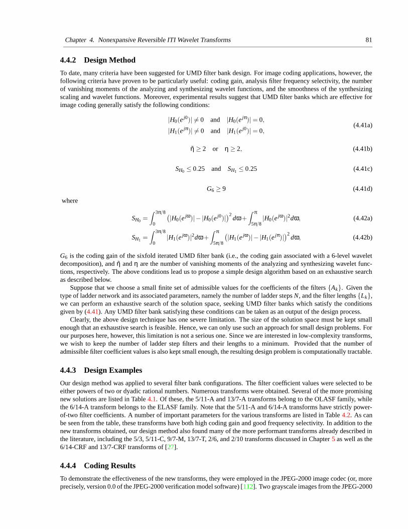
Chapter 4. Nonexpansive Reversible ITI Wavelet Transforms 81
4.4.2 Design Method
To date, many criteria have been suggested for UMD filter bank design. For image coding applications, however, thefollowing criteria have proven to be particularly useful: coding gain, analysis filter frequency selectivity, the numberof vanishing moments of the analyzing and synthesizing wavelet functions, and the smoothness of the synthesizingscaling and wavelet functions. Moreover, experimental results suggest that UMD filter banks which are effective forimage coding generally satisfy the following conditions:
|H0(ej0)| 6= 0 and |H0(e
jπ)| = 0,
|H1(ejπ)| 6= 0 and |H1(e
j0)| = 0,(4.41a)
η ≥ 2 or η ≥ 2, (4.41b)
SH0 ≤ 0.25 and SH1 ≤ 0.25 (4.41c)
G6 ≥ 9 (4.41d)
where
SH0 =∫ 3π/8
0
(|H0(e
jω)|− |H0(ej0)|)2
dω+∫ π
5π/8|H0(e
jω)|2dω, (4.42a)
SH1 =∫ 3π/8
0|H1(e
jω)|2dω+∫ π
5π/8
(|H1(e
jω)|− |H1(ejπ)|)2
dω, (4.42b)
G6 is the coding gain of the sixfold iterated UMD filter bank (i.e., the coding gain associated with a 6-level waveletdecomposition), and η and η are the number of vanishing moments of the analyzing and synthesizing wavelet func-tions, respectively. The above conditions lead us to propose a simple design algorithm based on an exhaustive searchas described below.
Suppose that we choose a small finite set of admissible values for the coefficients of the filters {Ak}. Given thetype of ladder network and its associated parameters, namely the number of ladder steps N, and the filter lengths {Lk},we can perform an exhaustive search of the solution space, seeking UMD filter banks which satisfy the conditionsgiven by (4.41). Any UMD filter bank satisfying these conditions can be taken as an output of the design process.
Clearly, the above design technique has one severe limitation. The size of the solution space must be kept smallenough that an exhaustive search is feasible. Hence, we can only use such an approach for small design problems. Forour purposes here, however, this limitation is not a serious one. Since we are interested in low-complexity transforms,we wish to keep the number of ladder step filters and their lengths to a minimum. Provided that the number ofadmissible filter coefficient values is also kept small enough, the resulting design problem is computationally tractable.
4.4.3 Design Examples
Our design method was applied to several filter bank configurations. The filter coefficient values were selected to beeither powers of two or dyadic rational numbers. Numerous transforms were obtained. Several of the more promisingnew solutions are listed in Table 4.1. Of these, the 5/11-A and 13/7-A transforms belong to the OLASF family, whilethe 6/14-A transform belongs to the ELASF family. Note that the 5/11-A and 6/14-A transforms have strictly power-of-two filter coefficients. A number of important parameters for the various transforms are listed in Table 4.2. As canbe seen from the table, these transforms have both high coding gain and good frequency selectivity. In addition to thenew transforms obtained, our design method also found many of the more performant transforms already described inthe literature, including the 5/3, 5/11-C, 9/7-M, 13/7-T, 2/6, and 2/10 transforms discussed in Chapter 5 as well as the6/14-CRF and 13/7-CRF transforms of [27].
4.4.4 Coding Results
To demonstrate the effectiveness of the new transforms, they were employed in the JPEG-2000 image codec (or, moreprecisely, version 0.0 of the JPEG-2000 verification model software) [112]. Two grayscale images from the JPEG-2000
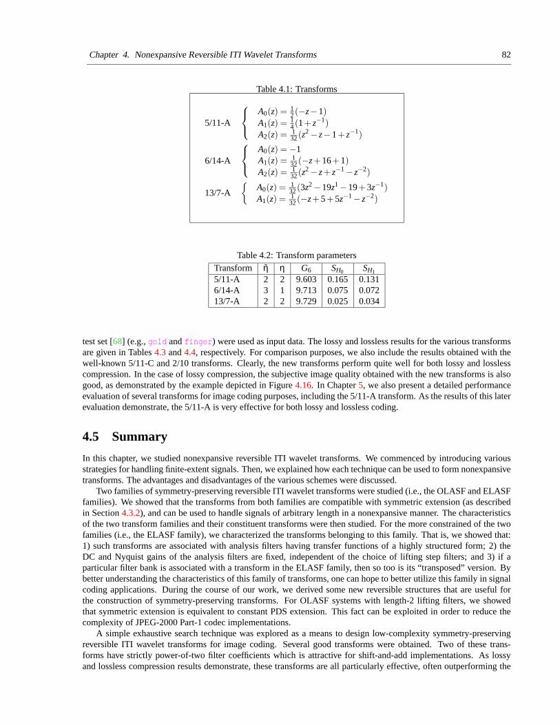
Chapter 4. Nonexpansive Reversible ITI Wavelet Transforms 82
Table 4.1: Transforms
5/11-A
A0(z) = 12 (−z−1)
A1(z) = 14 (1+ z−1)
A2(z) = 132 (z2 − z−1+ z−1)
6/14-A
A0(z) = −1A1(z) = 1
32 (−z+16+1)
A2(z) = 132 (z2 − z+ z−1 − z−2)
13/7-A
{A0(z) = 1
32 (3z2 −19z1 −19+3z−1)
A1(z) = 132 (−z+5+5z−1 − z−2)
Table 4.2: Transform parameters
Transform η η G6 SH0 SH1
5/11-A 2 2 9.603 0.165 0.1316/14-A 3 1 9.713 0.075 0.07213/7-A 2 2 9.729 0.025 0.034
test set [68] (e.g., gold and finger) were used as input data. The lossy and lossless results for the various transformsare given in Tables 4.3 and 4.4, respectively. For comparison purposes, we also include the results obtained with thewell-known 5/11-C and 2/10 transforms. Clearly, the new transforms perform quite well for both lossy and losslesscompression. In the case of lossy compression, the subjective image quality obtained with the new transforms is alsogood, as demonstrated by the example depicted in Figure 4.16. In Chapter 5, we also present a detailed performanceevaluation of several transforms for image coding purposes, including the 5/11-A transform. As the results of this laterevaluation demonstrate, the 5/11-A is very effective for both lossy and lossless coding.
4.5 Summary
In this chapter, we studied nonexpansive reversible ITI wavelet transforms. We commenced by introducing variousstrategies for handling finite-extent signals. Then, we explained how each technique can be used to form nonexpansivetransforms. The advantages and disadvantages of the various schemes were discussed.
Two families of symmetry-preserving reversible ITI wavelet transforms were studied (i.e., the OLASF and ELASFfamilies). We showed that the transforms from both families are compatible with symmetric extension (as describedin Section 4.3.2), and can be used to handle signals of arbitrary length in a nonexpansive manner. The characteristicsof the two transform families and their constituent transforms were then studied. For the more constrained of the twofamilies (i.e., the ELASF family), we characterized the transforms belonging to this family. That is, we showed that:1) such transforms are associated with analysis filters having transfer functions of a highly structured form; 2) theDC and Nyquist gains of the analysis filters are fixed, independent of the choice of lifting step filters; and 3) if aparticular filter bank is associated with a transform in the ELASF family, then so too is its “transposed” version. Bybetter understanding the characteristics of this family of transforms, one can hope to better utilize this family in signalcoding applications. During the course of our work, we derived some new reversible structures that are useful forthe construction of symmetry-preserving transforms. For OLASF systems with length-2 lifting filters, we showedthat symmetric extension is equivalent to constant PDS extension. This fact can be exploited in order to reduce thecomplexity of JPEG-2000 Part-1 codec implementations.
A simple exhaustive search technique was explored as a means to design low-complexity symmetry-preservingreversible ITI wavelet transforms for image coding. Several good transforms were obtained. Two of these trans-forms have strictly power-of-two filter coefficients which is attractive for shift-and-add implementations. As lossyand lossless compression results demonstrate, these transforms are all particularly effective, often outperforming the
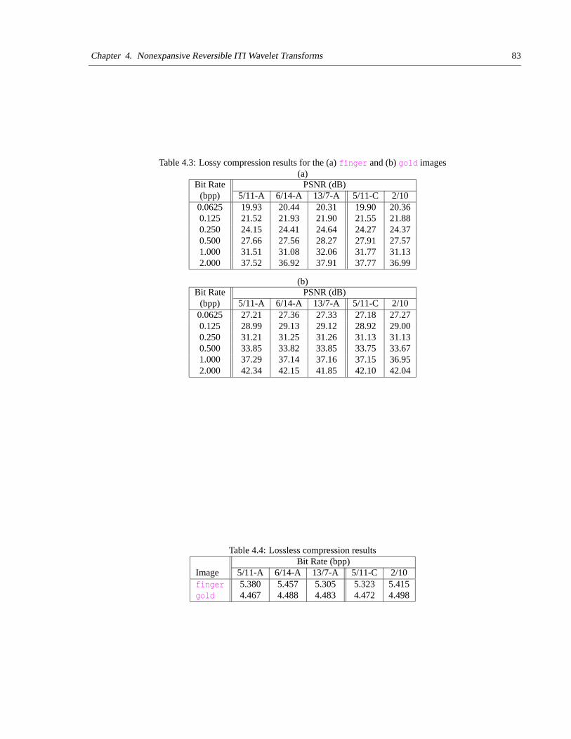
Chapter 4. Nonexpansive Reversible ITI Wavelet Transforms 83
Table 4.3: Lossy compression results for the (a) finger and (b) gold images(a)
Bit Rate PSNR (dB)(bpp) 5/11-A 6/14-A 13/7-A 5/11-C 2/10
0.0625 19.93 20.44 20.31 19.90 20.360.125 21.52 21.93 21.90 21.55 21.880.250 24.15 24.41 24.64 24.27 24.370.500 27.66 27.56 28.27 27.91 27.571.000 31.51 31.08 32.06 31.77 31.132.000 37.52 36.92 37.91 37.77 36.99
(b)Bit Rate PSNR (dB)
(bpp) 5/11-A 6/14-A 13/7-A 5/11-C 2/100.0625 27.21 27.36 27.33 27.18 27.270.125 28.99 29.13 29.12 28.92 29.000.250 31.21 31.25 31.26 31.13 31.130.500 33.85 33.82 33.85 33.75 33.671.000 37.29 37.14 37.16 37.15 36.952.000 42.34 42.15 41.85 42.10 42.04
Table 4.4: Lossless compression resultsBit Rate (bpp)
Image 5/11-A 6/14-A 13/7-A 5/11-C 2/10finger 5.380 5.457 5.305 5.323 5.415gold 4.467 4.488 4.483 4.472 4.498
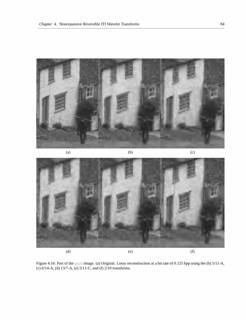
Chapter 4. Nonexpansive Reversible ITI Wavelet Transforms 84
(a) (b) (c)
(d) (e) (f)
Figure 4.16: Part of the gold image. (a) Original. Lossy reconstruction at a bit rate of 0.125 bpp using the (b) 5/11-A,(c) 6/14-A, (d) 13/7-A, (e) 5/11-C, and (f) 2/10 transforms.

Chapter 4. Nonexpansive Reversible ITI Wavelet Transforms 85
well-known 5/11-C and 2/10 transforms.
The world is a comedy to those who think and a tragedy to those who feel.
—Horace Walpole (1717–1797)
86
Chapter 5
Reversible ITI Wavelet Transforms forImage Coding
If it weren’t for the sadness it wouldn’t be so bad . . . If it were just the rage at my mother’s unchangedpersonality and my father’s unchanged silence, then it would be manageable. But my mother per-sists in making small, desperate, pathetic gestures of love; my father persists in attempting anunderstanding silence. It tears me apart. It makes me want to kill somebody or destroy somethingwhile simultaneously committing suicide. The sadness is unbearable, watching my parents try tocontain themselves, try not to do anything wrong or alienate me again. Yet their attempts are soobvious, clumsy, revealing all the more starkly what they are trying to hide. Their efforts fall short butare efforts nonetheless, and it makes me feel immensely sad, a sorrow that burns and washes inthe biggest fires and oceans. I want to protect them, throw my arms around them and demonstratetotal, self-sacrificing love. And I know that I can’t because it isn’t there.
—Evelyn Lau, Runaway: Diary of a Street Kid, 1989
Overview
In the context of image coding, a number of reversible ITI wavelet transforms are compared on the basis of theirlossy compression performance, lossless compression performance, and computational complexity. Of the transformsconsidered, several were found to perform particularly well, with the best choice for a given application depending onthe relative importance of the preceding criteria. Reversible ITI versions of numerous transforms are also comparedto their conventional (i.e., non-reversible real-to-real) counterparts for lossy compression. At low bit rates, reversibleITI and conventional versions of transforms were found to often yield results of comparable quality. Factors affectingthe compression performance of reversible ITI wavelet transforms are also presented, supported by both experimentaldata and theoretical arguments.
5.1 Introduction
The particular application of reversible ITI wavelet transforms considered in this thesis is image coding. In recentyears, reversible ITI wavelet transforms have become a popular tool for image coding applications. Transforms ofthis type are extremely useful for image compression systems requiring efficient handling of lossless coding, minimalmemory usage, or low computational complexity. Furthermore, such transforms are particularly attractive for sup-porting functionalities such as progressive lossy-to-lossless recovery of images, lossy compression with the losslessreproduction of a region of interest, and strictly lossy compression with minimal memory usage. Due to their utility,reversible ITI wavelet transforms have been adopted for use in the JPEG-2000 standard [72, 73, 19].
In this chapter, several reversible ITI wavelet transforms are compared on the basis of their lossy compressionperformance, lossless compression performance, and computational complexity. By using the results of such an eval-uation, not only are we able to build systems with improved compression efficiency, but we can also better understandthe tradeoffs between compression efficiency and computational complexity. Reversible ITI versions of transforms
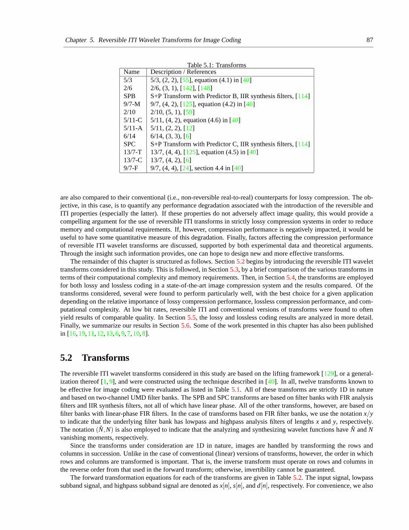
Chapter 5. Reversible ITI Wavelet Transforms for Image Coding 87
Table 5.1: TransformsName Description / References5/3 5/3, (2, 2), [55], equation (4.1) in [40]2/6 2/6, (3, 1), [142], [148]SPB S+P Transform with Predictor B, IIR synthesis filters, [114]9/7-M 9/7, (4, 2), [125], equation (4.2) in [40]2/10 2/10, (5, 1), [59]5/11-C 5/11, (4, 2), equation (4.6) in [40]5/11-A 5/11, (2, 2), [12]6/14 6/14, (3, 3), [6]SPC S+P Transform with Predictor C, IIR synthesis filters, [114]13/7-T 13/7, (4, 4), [125], equation (4.5) in [40]13/7-C 13/7, (4, 2), [6]9/7-F 9/7, (4, 4), [24], section 4.4 in [40]
are also compared to their conventional (i.e., non-reversible real-to-real) counterparts for lossy compression. The ob-jective, in this case, is to quantify any performance degradation associated with the introduction of the reversible andITI properties (especially the latter). If these properties do not adversely affect image quality, this would provide acompelling argument for the use of reversible ITI transforms in strictly lossy compression systems in order to reducememory and computational requirements. If, however, compression performance is negatively impacted, it would beuseful to have some quantitative measure of this degradation. Finally, factors affecting the compression performanceof reversible ITI wavelet transforms are discussed, supported by both experimental data and theoretical arguments.Through the insight such information provides, one can hope to design new and more effective transforms.
The remainder of this chapter is structured as follows. Section 5.2 begins by introducing the reversible ITI wavelettransforms considered in this study. This is followed, in Section 5.3, by a brief comparison of the various transforms interms of their computational complexity and memory requirements. Then, in Section 5.4, the transforms are employedfor both lossy and lossless coding in a state-of-the-art image compression system and the results compared. Of thetransforms considered, several were found to perform particularly well, with the best choice for a given applicationdepending on the relative importance of lossy compression performance, lossless compression performance, and com-putational complexity. At low bit rates, reversible ITI and conventional versions of transforms were found to oftenyield results of comparable quality. In Section 5.5, the lossy and lossless coding results are analyzed in more detail.Finally, we summarize our results in Section 5.6. Some of the work presented in this chapter has also been publishedin [16, 19, 11, 12, 13, 6, 9, 7, 10, 8].
5.2 Transforms
The reversible ITI wavelet transforms considered in this study are based on the lifting framework [129], or a general-ization thereof [1, 9], and were constructed using the technique described in [40]. In all, twelve transforms known tobe effective for image coding were evaluated as listed in Table 5.1. All of these transforms are strictly 1D in natureand based on two-channel UMD filter banks. The SPB and SPC transforms are based on filter banks with FIR analysisfilters and IIR synthesis filters, not all of which have linear phase. All of the other transforms, however, are based onfilter banks with linear-phase FIR filters. In the case of transforms based on FIR filter banks, we use the notation x/yto indicate that the underlying filter bank has lowpass and highpass analysis filters of lengths x and y, respectively.The notation (N,N) is also employed to indicate that the analyzing and synthesizing wavelet functions have N and Nvanishing moments, respectively.
Since the transforms under consideration are 1D in nature, images are handled by transforming the rows andcolumns in succession. Unlike in the case of conventional (linear) versions of transforms, however, the order in whichrows and columns are transformed is important. That is, the inverse transform must operate on rows and columns inthe reverse order from that used in the forward transform; otherwise, invertibility cannot be guaranteed.
The forward transformation equations for each of the transforms are given in Table 5.2. The input signal, lowpasssubband signal, and highpass subband signal are denoted as x[n], s[n], and d[n], respectively. For convenience, we also
Chapter 5. Reversible ITI Wavelet Transforms for Image Coding 88
define the quantities s0[n]4= x[2n] and d0[n]
4= x[2n+1]. The inverse transformation equations can be trivially deduced
from the forward transformation equations, and thus are not given here.When transforming finite-length signals, it is necessary to adopt some strategy for handling filtering at the signal
boundaries. In image coding applications, symmetric extension [33] is often employed for this purpose. To usesymmetric extension, however, the underlying filter bank must preserve signal symmetry. Although most of thetransforms considered here are derived from linear filter banks with linear-phase filters, this is not sufficient to ensurecompatibility with symmetric extension. Due to the rounding operations introduced in order to force a filter bank tomap integers to integers, the symmetry-preserving property is often lost.
In our study, one of two techniques for handling finite-length signals is employed, depending on the transform athand. In both instances, the method employed results in a nonexpansive transform for signals of arbitrary length. Incases where the underlying reversible ITI filter bank preserves signal symmetry, symmetric extension (as describedin Section 4.3.2) is used. More specifically, this strategy is employed in the case of the 5/3, 9/7-M, 5/11-C, 5/11-A, 13/7-T, 13/7-C, and 9/7-F transforms. In the case of the other transforms, constant PDS extension (described inSection 4.2.3) is employed. Periodic extension is avoided due to its poor performance in image coding applications.
Reversible ITI wavelet transforms approximate their parent linear transforms. For this reason, the characteristicsof the parent transforms are of great interest. In the case of linear wavelet transforms, a number of characteristics havebeen shown to potentially influence a transform’s effectiveness for coding purposes, including the number of vanishingmoments of the analyzing and synthesizing wavelet functions, the regularity of the analyzing and synthesizing scalingfunctions, coding gain, and the frequency selectivity of the analysis filters. These parameters are given for eachtransform in Table 5.3. Also of great importance is the shape of the synthesizing scaling and wavelet functions. It is theshape of these functions that ultimately determines the signals for which a transform is effective. In addition, the shapeof these functions determines the nature of the artifacts obtained in lossy signal reconstructions. The synthesizingscaling and wavelet functions for each transform are shown in Figures 5.1–5.12.
5.3 Computational Complexity and Memory Requirements
All of the reversible ITI wavelet transforms considered in this study are calculated using only fixed-point arithmetic.In particular, only integer addition/subtraction, multiplication, and division operations are required. Since all filtercoefficients are approximated by dyadic rational numbers, all division operations can be implemented as bit shifts. Forthe purposes of computational complexity analysis, we assume that the two’s complement representation for integersis used. By assuming a two’s complement representation, we can take advantage of the fact that
⌊x/2N
⌋is equivalent
to the arithmetic right shift of x by N bits (as shown much earlier in Proposition 4).Assuming a one-level wavelet decomposition (in one dimension), the number of addition, multiplication, and
shift operations required per two input samples for each transform is as given in Table 5.4. In each case, two setsof numbers are provided. The first set shows the number of operations in the straightforward implementation of thetransform. The second set, shown in parentheses, indicates the number of operations required if all multiplications areconverted to shift and add operations (via Booth’s algorithm [30]). This complexity metric is of particular interest forhardware implementations or software implementations on architectures where integer multiplications are more costlythan addition and shift operations. In the case where both sets of numbers are the same, only one is given. Symmetryin filter coefficients was considered in the calculation of these values.
Note that although a number of the transforms have equal operation counts, some require more multiplications thanothers. In particular, note that the 5/3, 2/6, 5/11-C and 5/11-A transforms are truly multiplierless (i.e., their underlyinglifting filters all have coefficients that are strictly powers of two). Evidently, the 5/3 and 2/6 transforms require theleast computation, followed by the SPB, 9/7-M, 2/10, 5/11-C, and 5/11-A transforms as a group, and then the 6/14,SPC, 13/7-T, and 13/7-C transforms as a group, and lastly the 9/7-F transform which requires the most computation.
As mentioned previously, reversible ITI versions of transforms have the potential for simpler implementationsthan their conventional counterparts. In the conventional case, all operands are real-valued. In the reversible ITI case,however, many operands are integers. Since, in both cases, approximately the same number of bits are required forthe integer part of numbers, it follows that more bits require processing in the conventional case. Thus, reversible ITItransforms can offer reduced computational complexity through a smaller wordsize for arithmetic operations.
The amount of memory needed by a transform-based coder can be strongly influenced by the amount of memoryrequired to store transform coefficients. In many image coding systems, transform coefficients are represented asreal numbers. Typically, in such systems, 32 bits of memory are needed to store each coefficient. Transforms which
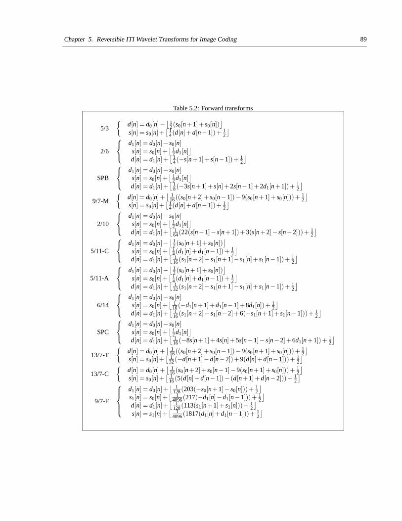
Chapter 5. Reversible ITI Wavelet Transforms for Image Coding 89
Table 5.2: Forward transforms
5/3
{d[n] = d0[n]−
⌊12 (s0[n+1]+ s0[n])
⌋
s[n] = s0[n]+⌊
14 (d[n]+d[n−1])+ 1
2
⌋
2/6
d1[n] = d0[n]− s0[n]s[n] = s0[n]+
⌊12 d1[n]
⌋
d[n] = d1[n]+⌊
14 (−s[n+1]+ s[n−1])+ 1
2
⌋
SPB
d1[n] = d0[n]− s0[n]s[n] = s0[n]+
⌊12 d1[n]
⌋
d[n] = d1[n]+⌊
18 (−3s[n+1]+ s[n]+2s[n−1]+2d1[n+1])+ 1
2
⌋
9/7-M
{d[n] = d0[n]+
⌊1
16 ((s0[n+2]+ s0[n−1])−9(s0[n+1]+ s0[n]))+ 12
⌋
s[n] = s0[n]+⌊
14 (d[n]+d[n−1])+ 1
2
⌋
2/10
d1[n] = d0[n]− s0[n]s[n] = s0[n]+
⌊12 d1[n]
⌋
d[n] = d1[n]+⌊
164 (22(s[n−1]− s[n+1])+3(s[n+2]− s[n−2]))+ 1
2
⌋
5/11-C
d1[n] = d0[n]−⌊
12 (s0[n+1]+ s0[n])
⌋
s[n] = s0[n]+⌊
14 (d1[n]+d1[n−1])+ 1
2
⌋
d[n] = d1[n]+⌊
116 (s1[n+2]− s1[n+1]− s1[n]+ s1[n−1])+ 1
2
⌋
5/11-A
d1[n] = d0[n]−⌊
12 (s0[n+1]+ s0[n])
⌋
s[n] = s0[n]+⌊
14 (d1[n]+d1[n−1])+ 1
2
⌋
d[n] = d1[n]+⌊
132 (s1[n+2]− s1[n+1]− s1[n]+ s1[n−1])+ 1
2
⌋
6/14
d1[n] = d0[n]− s0[n]s[n] = s0[n]+
⌊116 (−d1[n+1]+d1[n−1]+8d1[n])+ 1
2
⌋
d[n] = d1[n]+⌊
116 (s1[n+2]− s1[n−2]+6(−s1[n+1]+ s1[n−1]))+ 1
2
⌋
SPC
d1[n] = d0[n]− s0[n]s[n] = s0[n]+
⌊12 d1[n]
⌋
d[n] = d1[n]+⌊
116 (−8s[n+1]+4s[n]+5s[n−1]− s[n−2]+6d1[n+1])+ 1
2
⌋
13/7-T
{d[n] = d0[n]+
⌊1
16 ((s0[n+2]+ s0[n−1])−9(s0[n+1]+ s0[n]))+ 12
⌋
s[n] = s0[n]+⌊
132 (−d[n+1]−d[n−2])+9(d[n]+d[n−1]))+ 1
2
⌋
13/7-C
{d[n] = d0[n]+
⌊1
16 (s0[n+2]+ s0[n−1]−9(s0[n+1]+ s0[n]))+ 12
⌋
s[n] = s0[n]+⌊
116 (5(d[n]+d[n−1])− (d[n+1]+d[n−2]))+ 1
2
⌋
9/7-F
d1[n] = d0[n]+⌊
1128 (203(−s0[n+1]− s0[n]))+ 1
2
⌋
s1[n] = s0[n]+⌊
14096 (217(−d1[n]−d1[n−1]))+ 1
2
⌋
d[n] = d1[n]+⌊
1128 (113(s1[n+1]+ s1[n]))+ 1
2
⌋
s[n] = s1[n]+⌊
14096 (1817(d1[n]+d1[n−1]))+ 1
2
⌋
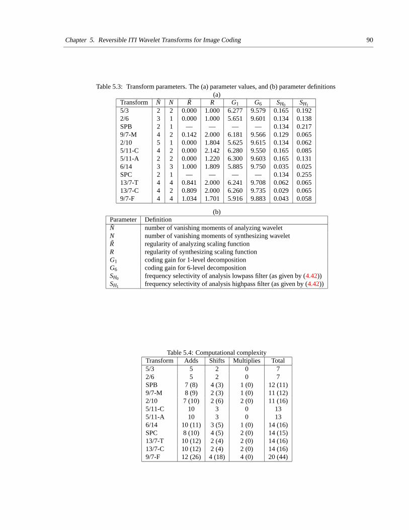
Chapter 5. Reversible ITI Wavelet Transforms for Image Coding 90
Table 5.3: Transform parameters. The (a) parameter values, and (b) parameter definitions(a)
Transform N N R R G1 G6 SH0 SH1
5/3 2 2 0.000 1.000 6.277 9.579 0.165 0.1922/6 3 1 0.000 1.000 5.651 9.601 0.134 0.138SPB 2 1 — — — — 0.134 0.2179/7-M 4 2 0.142 2.000 6.181 9.566 0.129 0.0652/10 5 1 0.000 1.804 5.625 9.615 0.134 0.0625/11-C 4 2 0.000 2.142 6.280 9.550 0.165 0.0855/11-A 2 2 0.000 1.220 6.300 9.603 0.165 0.1316/14 3 3 1.000 1.809 5.885 9.750 0.035 0.025SPC 2 1 — — — — 0.134 0.25513/7-T 4 4 0.841 2.000 6.241 9.708 0.062 0.06513/7-C 4 2 0.809 2.000 6.260 9.735 0.029 0.0659/7-F 4 4 1.034 1.701 5.916 9.883 0.043 0.058
(b)Parameter DefinitionN number of vanishing moments of analyzing waveletN number of vanishing moments of synthesizing waveletR regularity of analyzing scaling functionR regularity of synthesizing scaling functionG1 coding gain for 1-level decompositionG6 coding gain for 6-level decompositionSH0 frequency selectivity of analysis lowpass filter (as given by (4.42))SH1 frequency selectivity of analysis highpass filter (as given by (4.42))
Table 5.4: Computational complexityTransform Adds Shifts Multiplies Total5/3 5 2 0 72/6 5 2 0 7SPB 7 (8) 4 (3) 1 (0) 12 (11)9/7-M 8 (9) 2 (3) 1 (0) 11 (12)2/10 7 (10) 2 (6) 2 (0) 11 (16)5/11-C 10 3 0 135/11-A 10 3 0 136/14 10 (11) 3 (5) 1 (0) 14 (16)SPC 8 (10) 4 (5) 2 (0) 14 (15)13/7-T 10 (12) 2 (4) 2 (0) 14 (16)13/7-C 10 (12) 2 (4) 2 (0) 14 (16)9/7-F 12 (26) 4 (18) 4 (0) 20 (44)
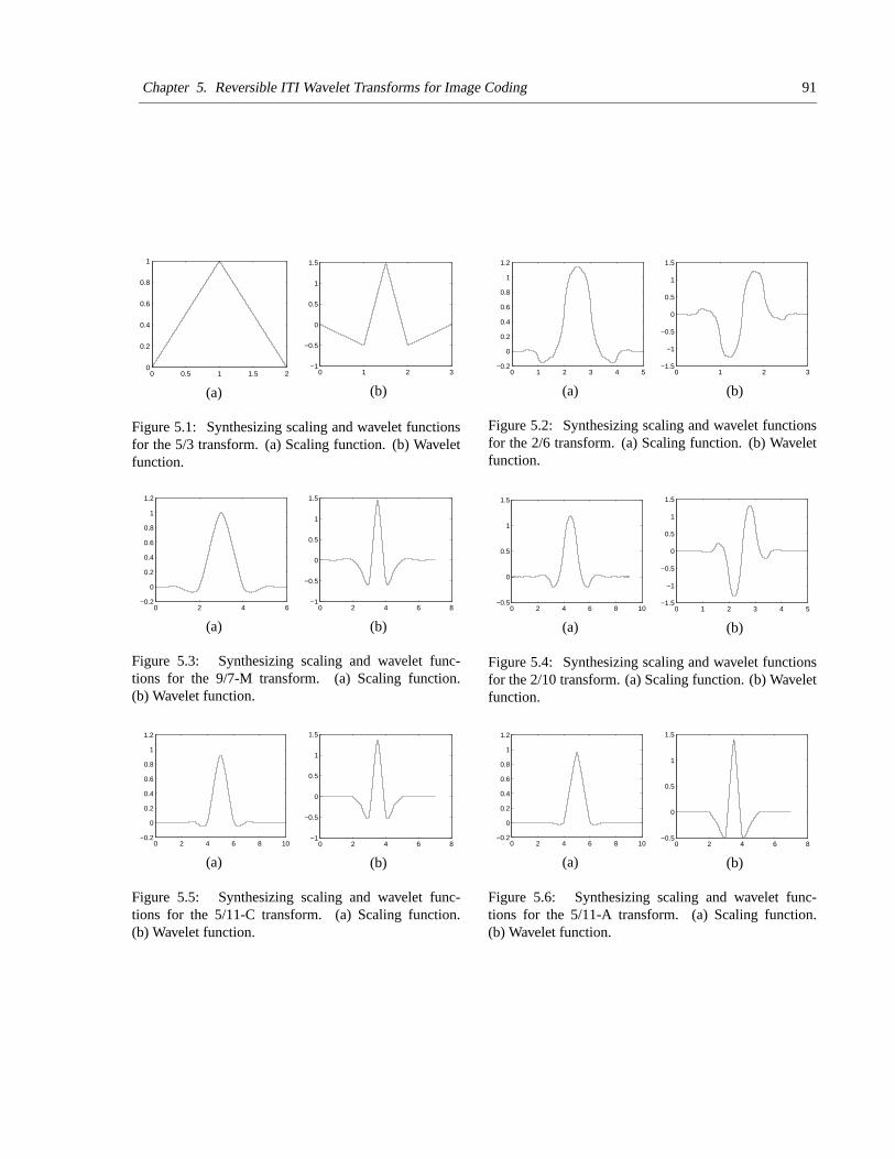
Chapter 5. Reversible ITI Wavelet Transforms for Image Coding 91
0 0.5 1 1.5 20
0.2
0.4
0.6
0.8
1
(a)
0 1 2 3−1
−0.5
0
0.5
1
1.5
(b)
Figure 5.1: Synthesizing scaling and wavelet functionsfor the 5/3 transform. (a) Scaling function. (b) Waveletfunction.
0 1 2 3 4 5−0.2
0
0.2
0.4
0.6
0.8
1
1.2
(a)
0 1 2 3−1.5
−1
−0.5
0
0.5
1
1.5
(b)
Figure 5.2: Synthesizing scaling and wavelet functionsfor the 2/6 transform. (a) Scaling function. (b) Waveletfunction.
0 2 4 6−0.2
0
0.2
0.4
0.6
0.8
1
1.2
(a)
0 2 4 6 8−1
−0.5
0
0.5
1
1.5
(b)
Figure 5.3: Synthesizing scaling and wavelet func-tions for the 9/7-M transform. (a) Scaling function.(b) Wavelet function.
0 2 4 6 8 10−0.5
0
0.5
1
1.5
(a)
0 1 2 3 4 5−1.5
−1
−0.5
0
0.5
1
1.5
(b)
Figure 5.4: Synthesizing scaling and wavelet functionsfor the 2/10 transform. (a) Scaling function. (b) Waveletfunction.
0 2 4 6 8 10−0.2
0
0.2
0.4
0.6
0.8
1
1.2
(a)
0 2 4 6 8−1
−0.5
0
0.5
1
1.5
(b)
Figure 5.5: Synthesizing scaling and wavelet func-tions for the 5/11-C transform. (a) Scaling function.(b) Wavelet function.
0 2 4 6 8 10−0.2
0
0.2
0.4
0.6
0.8
1
1.2
(a)
0 2 4 6 8−0.5
0
0.5
1
1.5
(b)
Figure 5.6: Synthesizing scaling and wavelet func-tions for the 5/11-A transform. (a) Scaling function.(b) Wavelet function.
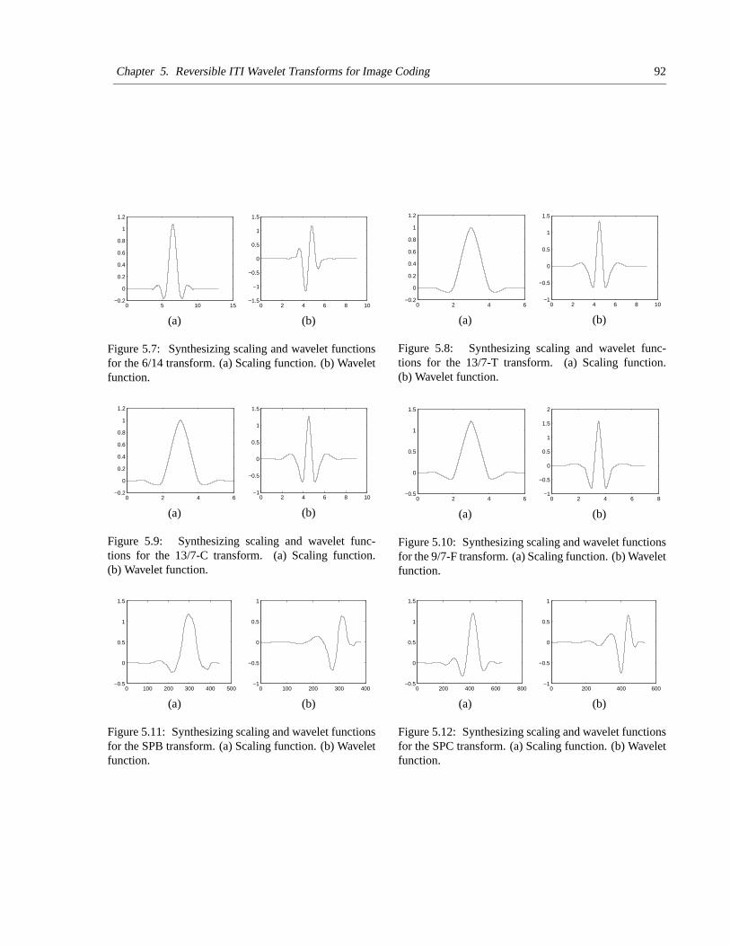
Chapter 5. Reversible ITI Wavelet Transforms for Image Coding 92
0 5 10 15−0.2
0
0.2
0.4
0.6
0.8
1
1.2
(a)
0 2 4 6 8 10−1.5
−1
−0.5
0
0.5
1
1.5
(b)
Figure 5.7: Synthesizing scaling and wavelet functionsfor the 6/14 transform. (a) Scaling function. (b) Waveletfunction.
0 2 4 6−0.2
0
0.2
0.4
0.6
0.8
1
1.2
(a)
0 2 4 6 8 10−1
−0.5
0
0.5
1
1.5
(b)
Figure 5.8: Synthesizing scaling and wavelet func-tions for the 13/7-T transform. (a) Scaling function.(b) Wavelet function.
0 2 4 6−0.2
0
0.2
0.4
0.6
0.8
1
1.2
(a)
0 2 4 6 8 10−1
−0.5
0
0.5
1
1.5
(b)
Figure 5.9: Synthesizing scaling and wavelet func-tions for the 13/7-C transform. (a) Scaling function.(b) Wavelet function.
0 2 4 6−0.5
0
0.5
1
1.5
(a)
0 2 4 6 8−1
−0.5
0
0.5
1
1.5
2
(b)
Figure 5.10: Synthesizing scaling and wavelet functionsfor the 9/7-F transform. (a) Scaling function. (b) Waveletfunction.
0 100 200 300 400 500−0.5
0
0.5
1
1.5
(a)
0 100 200 300 400−1
−0.5
0
0.5
1
(b)
Figure 5.11: Synthesizing scaling and wavelet functionsfor the SPB transform. (a) Scaling function. (b) Waveletfunction.
0 200 400 600 800−0.5
0
0.5
1
1.5
(a)
0 200 400 600−1
−0.5
0
0.5
1
(b)
Figure 5.12: Synthesizing scaling and wavelet functionsfor the SPC transform. (a) Scaling function. (b) Waveletfunction.
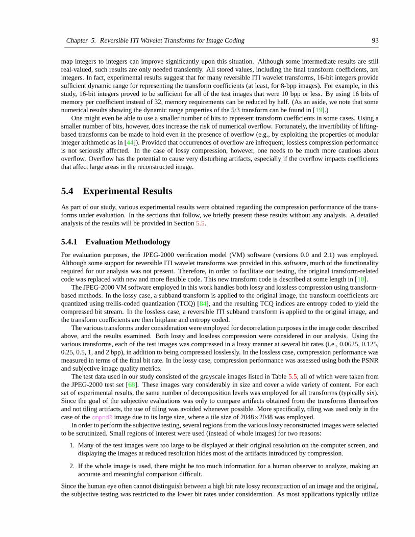
Chapter 5. Reversible ITI Wavelet Transforms for Image Coding 93
map integers to integers can improve significantly upon this situation. Although some intermediate results are stillreal-valued, such results are only needed transiently. All stored values, including the final transform coefficients, areintegers. In fact, experimental results suggest that for many reversible ITI wavelet transforms, 16-bit integers providesufficient dynamic range for representing the transform coefficients (at least, for 8-bpp images). For example, in thisstudy, 16-bit integers proved to be sufficient for all of the test images that were 10 bpp or less. By using 16 bits ofmemory per coefficient instead of 32, memory requirements can be reduced by half. (As an aside, we note that somenumerical results showing the dynamic range properties of the 5/3 transform can be found in [19].)
One might even be able to use a smaller number of bits to represent transform coefficients in some cases. Using asmaller number of bits, however, does increase the risk of numerical overflow. Fortunately, the invertibility of lifting-based transforms can be made to hold even in the presence of overflow (e.g., by exploiting the properties of modularinteger arithmetic as in [44]). Provided that occurrences of overflow are infrequent, lossless compression performanceis not seriously affected. In the case of lossy compression, however, one needs to be much more cautious aboutoverflow. Overflow has the potential to cause very disturbing artifacts, especially if the overflow impacts coefficientsthat affect large areas in the reconstructed image.
5.4 Experimental Results
As part of our study, various experimental results were obtained regarding the compression performance of the trans-forms under evaluation. In the sections that follow, we briefly present these results without any analysis. A detailedanalysis of the results will be provided in Section 5.5.
5.4.1 Evaluation Methodology
For evaluation purposes, the JPEG-2000 verification model (VM) software (versions 0.0 and 2.1) was employed.Although some support for reversible ITI wavelet transforms was provided in this software, much of the functionalityrequired for our analysis was not present. Therefore, in order to facilitate our testing, the original transform-relatedcode was replaced with new and more flexible code. This new transform code is described at some length in [10].
The JPEG-2000 VM software employed in this work handles both lossy and lossless compression using transform-based methods. In the lossy case, a subband transform is applied to the original image, the transform coefficients arequantized using trellis-coded quantization (TCQ) [84], and the resulting TCQ indices are entropy coded to yield thecompressed bit stream. In the lossless case, a reversible ITI subband transform is applied to the original image, andthe transform coefficients are then bitplane and entropy coded.
The various transforms under consideration were employed for decorrelation purposes in the image coder describedabove, and the results examined. Both lossy and lossless compression were considered in our analysis. Using thevarious transforms, each of the test images was compressed in a lossy manner at several bit rates (i.e., 0.0625, 0.125,0.25, 0.5, 1, and 2 bpp), in addition to being compressed losslessly. In the lossless case, compression performance wasmeasured in terms of the final bit rate. In the lossy case, compression performance was assessed using both the PSNRand subjective image quality metrics.
The test data used in our study consisted of the grayscale images listed in Table 5.5, all of which were taken fromthe JPEG-2000 test set [68]. These images vary considerably in size and cover a wide variety of content. For eachset of experimental results, the same number of decomposition levels was employed for all transforms (typically six).Since the goal of the subjective evaluations was only to compare artifacts obtained from the transforms themselvesand not tiling artifacts, the use of tiling was avoided whenever possible. More specifically, tiling was used only in thecase of the cmpnd2 image due to its large size, where a tile size of 2048×2048 was employed.
In order to perform the subjective testing, several regions from the various lossy reconstructed images were selectedto be scrutinized. Small regions of interest were used (instead of whole images) for two reasons:
1. Many of the test images were too large to be displayed at their original resolution on the computer screen, anddisplaying the images at reduced resolution hides most of the artifacts introduced by compression.
2. If the whole image is used, there might be too much information for a human observer to analyze, making anaccurate and meaningful comparison difficult.
Since the human eye often cannot distinguish between a high bit rate lossy reconstruction of an image and the original,the subjective testing was restricted to the lower bit rates under consideration. As most applications typically utilize

Chapter 5. Reversible ITI Wavelet Transforms for Image Coding 94
Table 5.5: Test imagesImage Size Depth Descriptionaerial2 2048×2048 8 aerial photographbike 2048×2560 8 collection of objectscafe 2048×2560 8 outside of cafecats 3072×2048 8 catschart 1688×2347 8 color chartcmpnd1 512×768 8 mixed text and graphicscmpnd2 5120×6624 8 mixed text and graphicscr 1744×2048 10 computer radiologyct 512×512 12 computer tomographyelev 1201×1201 12 fractal-like patternfinger 512×512 8 fingerprintgold 720×576 8 houses and countrysidehotel 720×576 8 hotelmat 1528×1146 8 mountainsmri 256×256 11 magnetic resonancesar1 1024×1024 16 synthetic aperture radarsar2 800×800 12 synthetic aperture radarseismic 512×512 8 seismic datatarget 512×512 8 patterns and texturestools 1524×1200 8 collection of toolstxtur1 1024×1024 8 aerial photographtxtur2 1024×1024 8 aerial photographus 512×448 8 ultrasoundwater 1465×1999 8 water and landwoman 2048×2560 8 ladyxray 2048×1680 12 x-ray
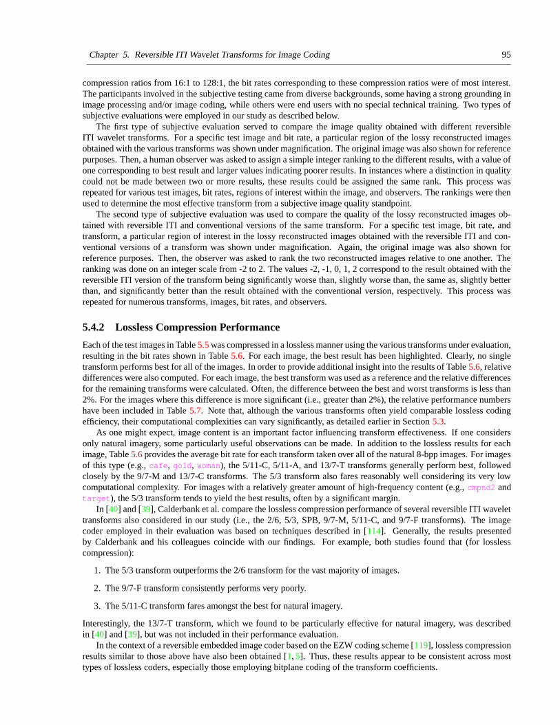
Chapter 5. Reversible ITI Wavelet Transforms for Image Coding 95
compression ratios from 16:1 to 128:1, the bit rates corresponding to these compression ratios were of most interest.The participants involved in the subjective testing came from diverse backgrounds, some having a strong grounding inimage processing and/or image coding, while others were end users with no special technical training. Two types ofsubjective evaluations were employed in our study as described below.
The first type of subjective evaluation served to compare the image quality obtained with different reversibleITI wavelet transforms. For a specific test image and bit rate, a particular region of the lossy reconstructed imagesobtained with the various transforms was shown under magnification. The original image was also shown for referencepurposes. Then, a human observer was asked to assign a simple integer ranking to the different results, with a value ofone corresponding to best result and larger values indicating poorer results. In instances where a distinction in qualitycould not be made between two or more results, these results could be assigned the same rank. This process wasrepeated for various test images, bit rates, regions of interest within the image, and observers. The rankings were thenused to determine the most effective transform from a subjective image quality standpoint.
The second type of subjective evaluation was used to compare the quality of the lossy reconstructed images ob-tained with reversible ITI and conventional versions of the same transform. For a specific test image, bit rate, andtransform, a particular region of interest in the lossy reconstructed images obtained with the reversible ITI and con-ventional versions of a transform was shown under magnification. Again, the original image was also shown forreference purposes. Then, the observer was asked to rank the two reconstructed images relative to one another. Theranking was done on an integer scale from -2 to 2. The values -2, -1, 0, 1, 2 correspond to the result obtained with thereversible ITI version of the transform being significantly worse than, slightly worse than, the same as, slightly betterthan, and significantly better than the result obtained with the conventional version, respectively. This process wasrepeated for numerous transforms, images, bit rates, and observers.
5.4.2 Lossless Compression Performance
Each of the test images in Table 5.5 was compressed in a lossless manner using the various transforms under evaluation,resulting in the bit rates shown in Table 5.6. For each image, the best result has been highlighted. Clearly, no singletransform performs best for all of the images. In order to provide additional insight into the results of Table 5.6, relativedifferences were also computed. For each image, the best transform was used as a reference and the relative differencesfor the remaining transforms were calculated. Often, the difference between the best and worst transforms is less than2%. For the images where this difference is more significant (i.e., greater than 2%), the relative performance numbershave been included in Table 5.7. Note that, although the various transforms often yield comparable lossless codingefficiency, their computational complexities can vary significantly, as detailed earlier in Section 5.3.
As one might expect, image content is an important factor influencing transform effectiveness. If one considersonly natural imagery, some particularly useful observations can be made. In addition to the lossless results for eachimage, Table 5.6 provides the average bit rate for each transform taken over all of the natural 8-bpp images. For imagesof this type (e.g., cafe, gold, woman), the 5/11-C, 5/11-A, and 13/7-T transforms generally perform best, followedclosely by the 9/7-M and 13/7-C transforms. The 5/3 transform also fares reasonably well considering its very lowcomputational complexity. For images with a relatively greater amount of high-frequency content (e.g., cmpnd2 andtarget), the 5/3 transform tends to yield the best results, often by a significant margin.
In [40] and [39], Calderbank et al. compare the lossless compression performance of several reversible ITI wavelettransforms also considered in our study (i.e., the 2/6, 5/3, SPB, 9/7-M, 5/11-C, and 9/7-F transforms). The imagecoder employed in their evaluation was based on techniques described in [114]. Generally, the results presentedby Calderbank and his colleagues coincide with our findings. For example, both studies found that (for losslesscompression):
1. The 5/3 transform outperforms the 2/6 transform for the vast majority of images.
2. The 9/7-F transform consistently performs very poorly.
3. The 5/11-C transform fares amongst the best for natural imagery.
Interestingly, the 13/7-T transform, which we found to be particularly effective for natural imagery, was describedin [40] and [39], but was not included in their performance evaluation.
In the context of a reversible embedded image coder based on the EZW coding scheme [119], lossless compressionresults similar to those above have also been obtained [1, 5]. Thus, these results appear to be consistent across mosttypes of lossless coders, especially those employing bitplane coding of the transform coefficients.
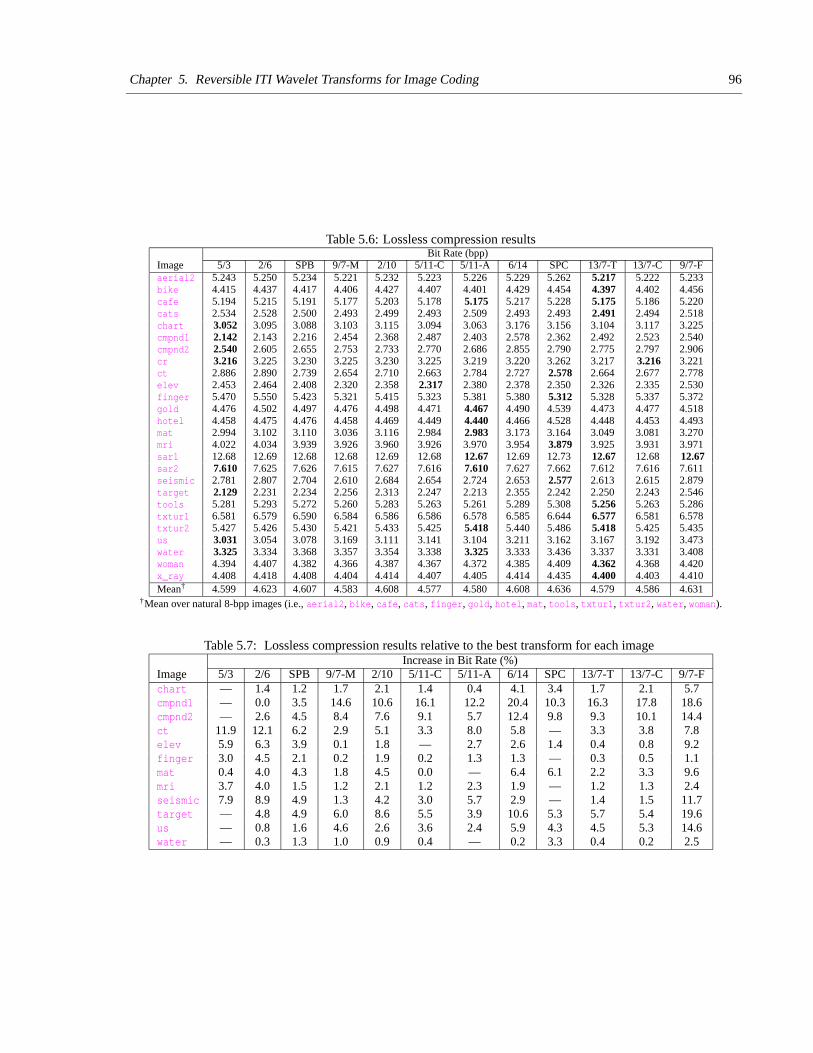
Chapter 5. Reversible ITI Wavelet Transforms for Image Coding 96
Table 5.6: Lossless compression resultsBit Rate (bpp)
Image 5/3 2/6 SPB 9/7-M 2/10 5/11-C 5/11-A 6/14 SPC 13/7-T 13/7-C 9/7-Faerial2 5.243 5.250 5.234 5.221 5.232 5.223 5.226 5.229 5.262 5.217 5.222 5.233bike 4.415 4.437 4.417 4.406 4.427 4.407 4.401 4.429 4.454 4.397 4.402 4.456cafe 5.194 5.215 5.191 5.177 5.203 5.178 5.175 5.217 5.228 5.175 5.186 5.220cats 2.534 2.528 2.500 2.493 2.499 2.493 2.509 2.493 2.493 2.491 2.494 2.518chart 3.052 3.095 3.088 3.103 3.115 3.094 3.063 3.176 3.156 3.104 3.117 3.225cmpnd1 2.142 2.143 2.216 2.454 2.368 2.487 2.403 2.578 2.362 2.492 2.523 2.540cmpnd2 2.540 2.605 2.655 2.753 2.733 2.770 2.686 2.855 2.790 2.775 2.797 2.906cr 3.216 3.225 3.230 3.225 3.230 3.225 3.219 3.220 3.262 3.217 3.216 3.221ct 2.886 2.890 2.739 2.654 2.710 2.663 2.784 2.727 2.578 2.664 2.677 2.778elev 2.453 2.464 2.408 2.320 2.358 2.317 2.380 2.378 2.350 2.326 2.335 2.530finger 5.470 5.550 5.423 5.321 5.415 5.323 5.381 5.380 5.312 5.328 5.337 5.372gold 4.476 4.502 4.497 4.476 4.498 4.471 4.467 4.490 4.539 4.473 4.477 4.518hotel 4.458 4.475 4.476 4.458 4.469 4.449 4.440 4.466 4.528 4.448 4.453 4.493mat 2.994 3.102 3.110 3.036 3.116 2.984 2.983 3.173 3.164 3.049 3.081 3.270mri 4.022 4.034 3.939 3.926 3.960 3.926 3.970 3.954 3.879 3.925 3.931 3.971sar1 12.68 12.69 12.68 12.68 12.69 12.68 12.67 12.69 12.73 12.67 12.68 12.67sar2 7.610 7.625 7.626 7.615 7.627 7.616 7.610 7.627 7.662 7.612 7.616 7.611seismic 2.781 2.807 2.704 2.610 2.684 2.654 2.724 2.653 2.577 2.613 2.615 2.879target 2.129 2.231 2.234 2.256 2.313 2.247 2.213 2.355 2.242 2.250 2.243 2.546tools 5.281 5.293 5.272 5.260 5.283 5.263 5.261 5.289 5.308 5.256 5.263 5.286txtur1 6.581 6.579 6.590 6.584 6.586 6.586 6.578 6.585 6.644 6.577 6.581 6.578txtur2 5.427 5.426 5.430 5.421 5.433 5.425 5.418 5.440 5.486 5.418 5.425 5.435us 3.031 3.054 3.078 3.169 3.111 3.141 3.104 3.211 3.162 3.167 3.192 3.473water 3.325 3.334 3.368 3.357 3.354 3.338 3.325 3.333 3.436 3.337 3.331 3.408woman 4.394 4.407 4.382 4.366 4.387 4.367 4.372 4.385 4.409 4.362 4.368 4.420x_ray 4.408 4.418 4.408 4.404 4.414 4.407 4.405 4.414 4.435 4.400 4.403 4.410Mean† 4.599 4.623 4.607 4.583 4.608 4.577 4.580 4.608 4.636 4.579 4.586 4.631
†Mean over natural 8-bpp images (i.e., aerial2, bike, cafe, cats, finger, gold, hotel, mat, tools, txtur1, txtur2, water, woman).
Table 5.7: Lossless compression results relative to the best transform for each imageIncrease in Bit Rate (%)
Image 5/3 2/6 SPB 9/7-M 2/10 5/11-C 5/11-A 6/14 SPC 13/7-T 13/7-C 9/7-Fchart — 1.4 1.2 1.7 2.1 1.4 0.4 4.1 3.4 1.7 2.1 5.7cmpnd1 — 0.0 3.5 14.6 10.6 16.1 12.2 20.4 10.3 16.3 17.8 18.6cmpnd2 — 2.6 4.5 8.4 7.6 9.1 5.7 12.4 9.8 9.3 10.1 14.4ct 11.9 12.1 6.2 2.9 5.1 3.3 8.0 5.8 — 3.3 3.8 7.8elev 5.9 6.3 3.9 0.1 1.8 — 2.7 2.6 1.4 0.4 0.8 9.2finger 3.0 4.5 2.1 0.2 1.9 0.2 1.3 1.3 — 0.3 0.5 1.1mat 0.4 4.0 4.3 1.8 4.5 0.0 — 6.4 6.1 2.2 3.3 9.6mri 3.7 4.0 1.5 1.2 2.1 1.2 2.3 1.9 — 1.2 1.3 2.4seismic 7.9 8.9 4.9 1.3 4.2 3.0 5.7 2.9 — 1.4 1.5 11.7target — 4.8 4.9 6.0 8.6 5.5 3.9 10.6 5.3 5.7 5.4 19.6us — 0.8 1.6 4.6 2.6 3.6 2.4 5.9 4.3 4.5 5.3 14.6water — 0.3 1.3 1.0 0.9 0.4 — 0.2 3.3 0.4 0.2 2.5
Chapter 5. Reversible ITI Wavelet Transforms for Image Coding 97
5.4.3 PSNR Lossy Compression Performance
Each of the test images in Table 5.5 was compressed in a lossy manner at several bit rates using the various transformsunder evaluation. The image quality was then measured using the PSNR metric as defined by (2.29). The results for arepresentative subset of the test images are given in Table 5.8. For each test image and bit rate pair, the best result hasbeen highlighted.
For low bit rates (i.e., compression ratios of 16:1 or greater), the 9/7-F, 6/14, 13/7-C, and 13/7-T transformsare consistently the best performers in approximately that order. The SPC and SPB transforms fare the worst. Asthe bit rate increases, lossy compression performance becomes increasing influenced by the lossless performancecharacteristics of the transforms. These results will be revisited later in Section 5.5.2 for analysis purposes.
In applications where lossy image reconstructions are processed by a computer system (e.g., some scientific ap-plications), the use of a distortion metric based on the mean-squared error (i.e., PSNR) can be quite appropriate.Unfortunately, the PSNR can be a poor measure of image quality for applications in which images are to be viewedby humans. Hence, a subjective evaluation, the results of which are presented in the next section, was necessary.
5.4.4 Subjective Lossy Compression Performance
Since the PSNR does not necessarily correlate well with image quality as perceived by the human visual system, wesupplemented our PSNR results with a subjective evaluation. This subjective testing was undertaken as specified inSection 5.4.1. In order to make the testing more practical, the evaluation was divided into two stages. The same testingstrategy was used in each stage. Only the transforms under evaluation in each case differed.
In the first stage, the 5/3, 2/6, SPB, 9/7-M, 2/10, SPC, 13/7-T, and 9/7-F transforms were compared. After obtainingthe rankings for 14 sets of images using 12 observers, these results were averaged together to yield the overall rankingsgiven in Table 5.9. From these results, we see that the transforms fall into three distinct performance categories. The9/7-F, 5/3, 13/7-T, and 9/7-M transforms perform best, followed by the 2/6 and 2/10 transforms, followed by theSPB and SPC transforms. These numerical results generally agree with comments made by participants during thesubjective tests—namely, that the transforms fall into three distinct performance categories.
The second stage of subjective testing included some of the best transforms from the first stage and several newtransforms, resulting in the following set of transforms: 5/3, 9/7-M, 5/11-C, 5/11-A, 6/14, 13/7-T, and 13/7-C. Afterconducting the subjective tests with 14 sets of images and 12 observers, the rankings were averaged together with theresults shown in Table 5.10. In this round of tests, the general consensus amongst the test participants is that all ofthe transforms are very close in terms of subjective quality, with the possible exception of the 6/14 transform whichperforms slightly worse. In other words, although the average rankings may differ by a large amount in this stage ofthe testing, it is important to note that even large disparities correspond to very minute differences in subjective imagequality.
Considering the results from both stages of the subjective testing, we conclude that the 9/7-F, 5/3, 13/7-T, 13/7-C,5/11-C, 5/11-A, and 9/7-M transforms have the best performance, followed by the 6/14, 2/6, and 2/10 transforms,followed by the SPB and SPC transforms. Examples of the quality obtained with transforms from each performancecategory are shown in Figure 5.13. We will again revisit these results in Section 5.5.2 where they will be examined inmore detail.
5.4.5 Reversible ITI Versus Conventional Transforms for Lossy Compression
Using both reversible ITI and conventional versions of the transforms listed in Table 5.1, the test images in Table 5.5were compressed in a lossy manner at several bit rates. The reconstructed images obtained with the two differentversions of each transform were then compared. The difference in the PSNR for a representative subset of the imagesis given in Table 5.11. A negative value corresponds to poorer performance in the reversible ITI transform case. As isevident from these results, the performance is almost always degraded in terms of PSNR in the reversible ITI transformcase, although the degradation is often very small. These numerical results also suggest some other important trendsthat will be discussed later in Section 5.5.1.
Subjective testing was also undertaken to compare the quality of the lossy image reconstructions obtained withreversible ITI and conventional versions of transforms. This testing was performed as described previously in Sec-tion 5.4.1. Due to the time consuming nature of subjective testing, only a subset of the transforms listed in Table 5.1was used, namely the 5/3, 2/6, SPB, 9/7-M, 2/10, SPC, 13/7-T, and 9/7-F transforms. After averaging the scores

Chapter 5. Reversible ITI Wavelet Transforms for Image Coding 98
Table 5.8: Lossy compression results for (a) aerial2, (b) bike, (c) cafe, (d) sar2, and (e) target images(a)
Bit Rate PSNR (dB)(bpp) 5/3 2/6 SPB 9/7-M 2/10 5/11-C 5/11-A 6/14 SPC 13/7-T 13/7-C 9/7-F
0.0625 24.40 24.47 24.05 24.46 24.55 24.41 24.45 24.66 23.63 24.60 24.64 24.720.1250 26.24 26.31 25.83 26.36 26.42 26.30 26.33 26.53 25.35 26.50 26.54 26.590.2500 28.15 28.25 27.49 28.35 28.37 28.26 28.25 28.53 26.91 28.50 28.55 28.600.5000 30.36 30.37 29.25 30.49 30.48 30.47 30.45 30.68 28.54 30.62 30.67 30.691.0000 33.30 33.30 31.89 33.35 33.31 33.34 33.36 33.54 30.97 33.50 33.53 33.502.0000 38.55 38.51 36.74 38.46 38.52 38.45 38.53 38.56 35.72 38.56 38.58 38.13
(b)Bit Rate PSNR (dB)
(bpp) 5/3 2/6 SPB 9/7-M 2/10 5/11-C 5/11-A 6/14 SPC 13/7-T 13/7-C 9/7-F0.0625 22.49 22.63 22.16 22.61 22.70 22.59 22.52 22.88 21.60 22.78 22.85 22.950.1250 25.03 25.26 24.63 25.12 25.32 25.03 25.08 25.47 24.02 25.34 25.41 25.580.2500 28.27 28.34 27.84 28.31 28.37 28.21 28.31 28.56 27.17 28.57 28.62 28.760.5000 32.27 32.24 31.59 32.23 32.18 32.13 32.29 32.33 30.77 32.30 32.51 32.571.0000 36.97 36.87 35.60 36.85 36.74 36.82 36.95 36.87 34.76 37.04 37.06 36.832.0000 42.77 42.57 40.55 42.42 42.43 42.48 42.70 42.35 39.49 42.47 42.42 41.12
(c)Bit Rate PSNR (dB)
(bpp) 5/3 2/6 SPB 9/7-M 2/10 5/11-C 5/11-A 6/14 SPC 13/7-T 13/7-C 9/7-F0.0625 18.77 18.89 18.17 18.78 18.88 18.72 18.77 18.99 17.61 18.92 18.97 19.040.1250 20.29 20.47 19.77 20.30 20.45 20.25 20.29 20.59 19.14 20.45 20.50 20.620.2500 22.75 22.90 22.10 22.75 22.89 22.72 22.77 23.03 21.39 22.94 22.98 23.120.5000 26.33 26.31 25.56 26.36 26.30 26.32 26.39 26.43 24.81 26.55 26.56 26.641.0000 31.41 31.30 30.59 31.42 31.26 31.37 31.47 31.38 29.76 31.62 31.62 31.632.0000 38.62 38.42 36.98 38.41 38.32 38.39 38.58 38.33 35.98 38.52 38.49 38.06
(d)Bit Rate PSNR (dB)
(bpp) 5/3 2/6 SPB 9/7-M 2/10 5/11-C 5/11-A 6/14 SPC 13/7-T 13/7-C 9/7-F0.0625 22.21 22.33 21.77 22.22 22.34 22.18 22.21 22.41 21.31 22.32 22.34 22.420.1250 22.97 23.09 22.28 22.98 23.09 22.94 22.97 23.18 21.76 23.07 23.10 23.180.2500 23.99 24.12 23.06 23.95 24.13 23.93 23.97 24.25 22.44 24.09 24.13 24.260.5000 25.54 25.63 24.43 25.50 25.60 25.47 25.53 25.80 23.65 25.64 25.70 25.821.0000 28.22 28.44 27.08 28.08 28.35 28.12 28.20 28.54 26.03 28.32 28.38 28.552.0000 33.85 33.86 32.26 33.66 33.74 33.63 33.79 33.98 31.04 33.86 33.90 34.08
(e)Bit Rate PSNR (dB)
(bpp) 5/3 2/6 SPB 9/7-M 2/10 5/11-C 5/11-A 6/14 SPC 13/7-T 13/7-C 9/7-F0.0625 17.57 17.30 17.04 17.55 17.34 17.46 17.54 18.17 16.41 18.12 18.36 18.950.1250 19.89 19.44 18.12 20.20 19.34 19.99 19.98 20.45 17.54 20.73 21.05 20.970.2500 23.28 23.01 22.75 23.64 23.18 23.36 23.41 24.76 22.31 24.38 25.48 24.920.5000 29.98 29.30 28.81 30.73 29.74 30.64 30.55 31.15 28.49 31.76 32.51 31.821.0000 41.38 40.03 37.99 41.25 39.79 41.04 40.99 40.68 37.69 41.70 41.94 40.212.0000 54.14 54.79 50.79 52.26 52.91 52.07 52.37 52.22 48.42 52.13 51.78 44.60
Table 5.9: Overall subjective rankings from first stage of testingRank
5/3 2/6 SPB 9/7-M 2/10 SPC 13/7-T 9/7-F2.51 4.47 6.05 2.97 4.57 6.88 2.88 2.36
Table 5.10: Overall subjective rankings from second stage of testingRank
5/3 9/7-M 5/11-C 5/11-A 6/14 13/7-T 13/7-C1.84 2.30 2.34 2.15 2.75 1.77 1.83
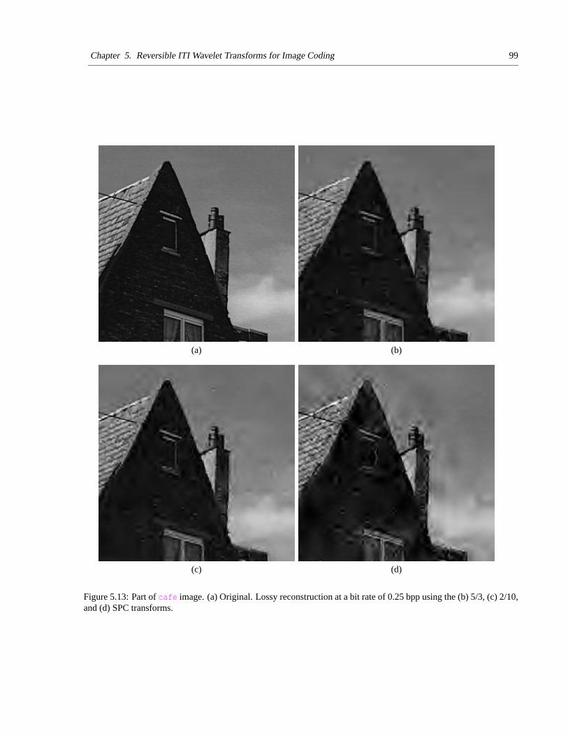
Chapter 5. Reversible ITI Wavelet Transforms for Image Coding 99
(a) (b)
(c) (d)
Figure 5.13: Part of cafe image. (a) Original. Lossy reconstruction at a bit rate of 0.25 bpp using the (b) 5/3, (c) 2/10,and (d) SPC transforms.

Chapter 5. Reversible ITI Wavelet Transforms for Image Coding 100
Table 5.11: Difference in PSNR performance between reversible ITI and conventional versions of transforms for the(a) aerial2, (b) bike, (c) cafe, (d) sar2, and (e) target images
(a)Bit Rate PSNR (dB)
(bpp) 5/3 2/6 SPB 9/7-M 2/10 5/11-C 5/11-A 6/14 SPC 13/7-T 13/7-C 9/7-F0.0625 -0.03 -0.04 -0.54 -0.05 -0.04 -0.03 -0.03 -0.05 -0.69 -0.03 -0.03 -0.030.1250 -0.05 -0.06 -0.64 -0.06 -0.07 -0.06 -0.04 -0.06 -0.84 -0.05 -0.02 -0.080.2500 -0.14 -0.09 -0.96 -0.10 -0.10 -0.15 -0.07 -0.10 -1.29 -0.09 -0.09 -0.080.5000 -0.09 -0.14 -1.31 -0.13 -0.16 -0.13 -0.11 -0.15 -1.63 -0.15 -0.15 -0.16
(b)Bit Rate PSNR (dB)
(bpp) 5/3 2/6 SPB 9/7-M 2/10 5/11-C 5/11-A 6/14 SPC 13/7-T 13/7-C 9/7-F0.0625 -0.02 -0.02 -0.52 -0.02 -0.03 -0.02 -0.02 -0.02 -0.70 -0.02 -0.02 -0.010.1250 -0.04 -0.06 -0.75 -0.05 -0.05 -0.05 -0.05 -0.05 -0.94 -0.04 -0.05 -0.020.2500 -0.08 -0.09 -0.71 -0.10 -0.10 -0.10 -0.08 -0.09 -0.87 -0.09 -0.10 -0.070.5000 -0.16 -0.21 -0.99 -0.20 -0.23 -0.21 -0.16 -0.22 -1.16 -0.36 -0.22 -0.24
(c)Bit Rate PSNR (dB)
(bpp) 5/3 2/6 SPB 9/7-M 2/10 5/11-C 5/11-A 6/14 SPC 13/7-T 13/7-C 9/7-F0.0625 -0.01 -0.01 -0.62 -0.01 -0.01 -0.01 -0.01 -0.01 -0.84 -0.01 -0.00 -0.010.1250 -0.01 -0.02 -0.68 -0.01 -0.02 -0.01 -0.01 -0.01 -0.86 -0.01 -0.01 -0.010.2500 -0.02 -0.03 -0.82 -0.04 -0.03 -0.03 -0.03 -0.02 -1.00 -0.03 -0.02 0.020.5000 -0.05 -0.06 -0.91 -0.06 -0.07 -0.07 -0.06 -0.07 -0.94 -0.05 -0.07 -0.07
(d)Bit Rate PSNR (dB)
(bpp) 5/3 2/6 SPB 9/7-M 2/10 5/11-C 5/11-A 6/14 SPC 13/7-T 13/7-C 9/7-F0.0625 -0.01 -0.00 -0.54 -0.00 -0.00 0.00 -0.00 0.00 -0.79 -0.00 0.00 -0.000.1250 -0.00 -0.00 -0.76 -0.00 -0.00 0.00 -0.00 -0.00 -1.05 -0.00 -0.00 -0.000.2500 0.03 -0.00 -0.97 0.00 -0.00 -0.00 0.00 -0.00 -1.24 0.00 -0.00 0.000.5000 -0.00 -0.03 -1.10 -0.00 -0.00 -0.00 -0.00 -0.00 -1.37 -0.00 -0.00 0.001.0000 -0.00 0.00 -1.15 -0.07 0.00 -0.00 -0.00 -0.00 -1.36 -0.00 0.07 -0.002.0000 -0.00 -0.01 -1.27 -0.00 -0.00 -0.00 -0.01 -0.00 -1.39 -0.00 0.00 0.00
(e)Bit Rate PSNR (dB)
(bpp) 5/3 2/6 SPB 9/7-M 2/10 5/11-C 5/11-A 6/14 SPC 13/7-T 13/7-C 9/7-F0.0625 0.01 -0.05 -0.34 -0.01 -0.03 0.01 0.02 0.08 -0.69 -0.01 -0.01 0.050.1250 0.00 0.03 -1.01 -0.00 -0.14 -0.03 -0.02 -0.06 -1.12 -0.00 -0.11 -0.070.2500 0.00 -0.35 -0.28 -0.02 -0.12 -0.03 -0.03 -0.01 -0.87 -0.02 -0.03 -0.030.5000 -0.05 -0.25 -1.20 -0.11 -0.14 -0.14 -0.13 -0.11 -1.55 -0.20 -0.17 -0.33
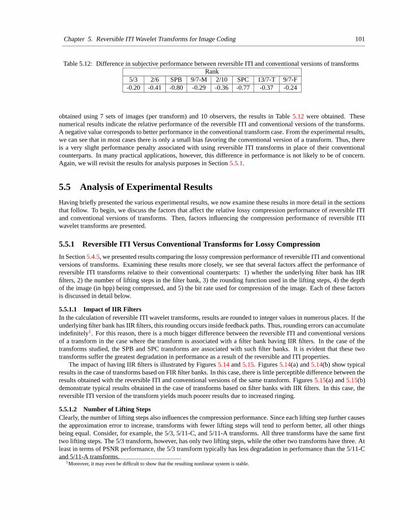
Chapter 5. Reversible ITI Wavelet Transforms for Image Coding 101
Table 5.12: Difference in subjective performance between reversible ITI and conventional versions of transformsRank
5/3 2/6 SPB 9/7-M 2/10 SPC 13/7-T 9/7-F-0.20 -0.41 -0.80 -0.29 -0.36 -0.77 -0.37 -0.24
obtained using 7 sets of images (per transform) and 10 observers, the results in Table 5.12 were obtained. Thesenumerical results indicate the relative performance of the reversible ITI and conventional versions of the transforms.A negative value corresponds to better performance in the conventional transform case. From the experimental results,we can see that in most cases there is only a small bias favoring the conventional version of a transform. Thus, thereis a very slight performance penalty associated with using reversible ITI transforms in place of their conventionalcounterparts. In many practical applications, however, this difference in performance is not likely to be of concern.Again, we will revisit the results for analysis purposes in Section 5.5.1.
5.5 Analysis of Experimental Results
Having briefly presented the various experimental results, we now examine these results in more detail in the sectionsthat follow. To begin, we discuss the factors that affect the relative lossy compression performance of reversible ITIand conventional versions of transforms. Then, factors influencing the compression performance of reversible ITIwavelet transforms are presented.
5.5.1 Reversible ITI Versus Conventional Transforms for Lossy Compression
In Section 5.4.5, we presented results comparing the lossy compression performance of reversible ITI and conventionalversions of transforms. Examining these results more closely, we see that several factors affect the performance ofreversible ITI transforms relative to their conventional counterparts: 1) whether the underlying filter bank has IIRfilters, 2) the number of lifting steps in the filter bank, 3) the rounding function used in the lifting steps, 4) the depthof the image (in bpp) being compressed, and 5) the bit rate used for compression of the image. Each of these factorsis discussed in detail below.
5.5.1.1 Impact of IIR FiltersIn the calculation of reversible ITI wavelet transforms, results are rounded to integer values in numerous places. If theunderlying filter bank has IIR filters, this rounding occurs inside feedback paths. Thus, rounding errors can accumulateindefinitely1. For this reason, there is a much bigger difference between the reversible ITI and conventional versionsof a transform in the case where the transform is associated with a filter bank having IIR filters. In the case of thetransforms studied, the SPB and SPC transforms are associated with such filter banks. It is evident that these twotransforms suffer the greatest degradation in performance as a result of the reversible and ITI properties.
The impact of having IIR filters is illustrated by Figures 5.14 and 5.15. Figures 5.14(a) and 5.14(b) show typicalresults in the case of transforms based on FIR filter banks. In this case, there is little perceptible difference between theresults obtained with the reversible ITI and conventional versions of the same transform. Figures 5.15(a) and 5.15(b)demonstrate typical results obtained in the case of transforms based on filter banks with IIR filters. In this case, thereversible ITI version of the transform yields much poorer results due to increased ringing.
5.5.1.2 Number of Lifting StepsClearly, the number of lifting steps also influences the compression performance. Since each lifting step further causesthe approximation error to increase, transforms with fewer lifting steps will tend to perform better, all other thingsbeing equal. Consider, for example, the 5/3, 5/11-C, and 5/11-A transforms. All three transforms have the same firsttwo lifting steps. The 5/3 transform, however, has only two lifting steps, while the other two transforms have three. Atleast in terms of PSNR performance, the 5/3 transform typically has less degradation in performance than the 5/11-Cand 5/11-A transforms.
1Moreover, it may even be difficult to show that the resulting nonlinear system is stable.
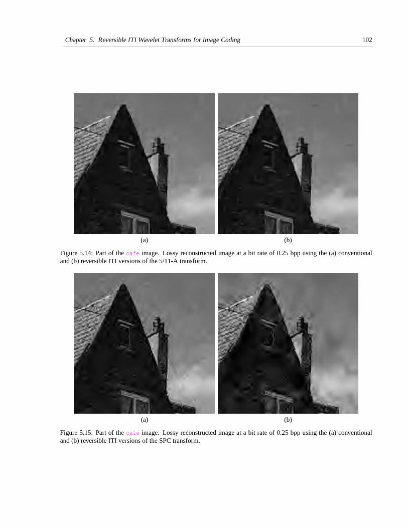
Chapter 5. Reversible ITI Wavelet Transforms for Image Coding 102
(a) (b)
Figure 5.14: Part of the cafe image. Lossy reconstructed image at a bit rate of 0.25 bpp using the (a) conventionaland (b) reversible ITI versions of the 5/11-A transform.
(a) (b)
Figure 5.15: Part of the cafe image. Lossy reconstructed image at a bit rate of 0.25 bpp using the (a) conventionaland (b) reversible ITI versions of the SPC transform.
Chapter 5. Reversible ITI Wavelet Transforms for Image Coding 103
5.5.1.3 Rounding FunctionThe function used to round results to integer values also affects the difference in performance between reversible ITItransforms and their conventional counterparts. In this study, we chose to use a biased floor function (i.e., Q(x) =⌊x+ 1
2
⌋) for this purpose. One could conceivably remove the bias of one-half, however. Such a change would reduce
computational complexity at the expense of introducing systematic error. The resulting performance degradation atlow bit rates is typically small. At higher bit rates, however, the degradation can be more significant, especially in thecase of lossless compression.
5.5.1.4 Depth of ImageAs the dynamic range of the signal grows, the errors introduced by rounding various results to integer values arerelatively smaller. For 8-bpp images there is a clear difference in PSNR performance between the reversible ITI andconventional versions of a transform, especially at higher bit rates. In the case of 12-bpp images (e.g., sar2), however,there is little difference in performance provided that the transforms are based on FIR filter banks.
5.5.1.5 Bit RateAs the bit rate is lowered, the difference in compression performance between reversible ITI and conventional versionsof a transform decreases. At a sufficiently low bit rate, the quantization of transform coefficients becomes so coarsethat any errors introduced by rounding intermediate results to integers are masked by quantization of the coefficientsthemselves.
5.5.2 Factors Affecting Compression Performance
In our study, three factors were found to affect the compression performance of a reversible ITI wavelet transform:1) the performance characteristics of its parent linear transform, 2) how closely it is able to approximate its parentlinear transform, and 3) the dynamic range of the coefficients produced by the transform. The first two factors affectboth lossy and lossless compression performance. The last factor is typically only important in the case of losslesscompression performance. Each of these factors will be discussed in turn in the remainder of this section. Table 5.14lists several parameters for each transform relevant to compression performance. Comments about these parameterswill also be made at the appropriate point in the paragraphs that follow.
5.5.2.1 Parent Linear TransformThe first point above has been covered in depth by many researchers, and techniques for the design of linear wavelettransforms are plentiful in the literature. Some design considerations include: time and frequency resolution, numberof vanishing moments, regularity, and coding gain. The effectiveness of a particular transform is also to some extentsignal dependent.
Section 5.4.3 presented the PSNR lossy compression performance results for the various transforms. The 9/7-F,6/14, 13/7-C, and 13/7-T transforms were found to be most effective. Looking at parameter G6 in Table 5.3, we cansee that these four transforms also have the parent linear transforms with the highest coding gain. Thus, the codinggain of the parent linear transform is of great importance, as one might suspect.
In Section 5.4.4, the subjective lossy compression performance results for the various transforms were presented.To a large extent, the subjective performance of these transforms can be explained by examining the synthesizingscaling and wavelet functions of their parent linear transforms as shown in Figures 5.1–5.12. From these plots, we cansee that the 9/7-F, 13/7-T, 13/7-C, 5/11-C, 5/11-A, and 9/7-M transforms have very smooth synthesizing scaling andwavelet functions, leading to their favorable performance. In the case of the 5/3 transform, the scaling and waveletfunctions have discontinuities in their first derivatives. Since there are no oscillations or jump discontinuities in thesefunctions, however, the 5/3 transform is still able to perform very well. In fact, the 5/3 transform is especially attractiveas it often introduces less pronounced ringing artifacts than the other transforms due to its short filters. Althoughsometimes very good at preserving high frequency textures, the SPB and SPC transforms perform worst, due largelyto their tendency to introduce ringing artifacts. This behavior can be attributed to the fact that both transforms areassociated with filter banks having IIR synthesis filters. The 6/14 transform often introduces more ringing artifactsthan some of the other transforms, leading to its relatively poor performance. This ringing is associated with the greateroscillatory nature of the synthesizing wavelet and scaling functions. In the case of the 2/6 transform, blockiness oftenresults. This behavior can be attributed to the relatively rougher synthesizing scaling and wavelet functions associatedwith this transform. Lastly, the 2/10 transform often results in more pronounced ringing artifacts, leading to its poorerperformance. This behavior can be attributed to the larger support of the synthesizing scaling and wavelet functions.
Chapter 5. Reversible ITI Wavelet Transforms for Image Coding 104
Table 5.13: Influence of the number of lifting steps on lossless compression performance2 lifting steps 4 lifting steps
Bit Rate Bit RateImage MAE† (bpp) MAE† (bpp)gold 0.409 4.473 0.540 4.479target 0.216 2.250 0.295 2.311woman 0.415 4.362 0.536 4.373
†mean absolute error
5.5.2.2 Approximation BehaviorThe approximation characteristics of reversible ITI wavelet transforms have not been given much serious attention todate. This is, however, an important factor to consider. Clearly, even if a reversible ITI transform is derived froma linear transform with desirable properties, the extent to which these properties are present in the reversible ITItransform depends entirely on how well it approximates its parent transform. The predominant source of error is therounding of intermediate results to integers. This error depends on the rounding function employed, the number oflifting steps in which this rounding is performed, and whether recursive filtering structures are used.
The number of lifting steps associated with each transform is given in Table 5.14. In the case of lossless com-pression, most of the best transforms tend to have only two or three lifting steps. All other things being equal, as thenumber of lifting steps increases so too does the approximation error. In the lossy case, the approximation error is lesscritical. Unless the approximation error is very large, it is usually masked by the error introduced by transform coeffi-cient quantization. Notice in particular that the 9/7-F transform has the most lifting steps of the transforms considered,and it also has arguably the poorest lossless compression performance.
To further demonstrate the influence of the number of lifting steps on compression performance, we losslesslycompressed several images using two different versions of the 13/7-T transform. The first version of the transformis the one given in Table 5.2 which has two lifting steps. The second version has four lifting steps. In each case,we measured the lossless bit rate and average approximation error. As can be seen from the results in Table 5.13,the lossless compression performance is better for the version of the transform with two lifting steps. Note that theapproximation error is also lower in this case as well. This observation suggests that, all other things being equal,transforms with two lifting steps (i.e., interpolating transforms) may offer the most promise for lossless compression2.
5.5.2.3 Dynamic RangeIn the case of lossless compression, all bits of the transform coefficients must be encoded. Thus, as the dynamic rangeof the transform coefficients increases, so too does the number of bits required to encode these coefficients. For thisreason, dynamic range is an important factor affecting lossless compression performance. Typically, the coefficientsobtained by the application of a transform have a greater dynamic range than the original samples. This dynamic rangegrowth is, therefore, of concern. The worst-case dynamic range growth of a particular transform is an approximatefunction of the 1-norm of its analysis filters. The 1-norms of the lowpass and highpass analysis filters determinethe worst-case growth in the lowpass and highpass channels, respectively. As the 1-norms increase, the worst-casedynamic range growth also increases. For reference purposes in what follows, the analysis filter 1-norms for eachtransform are given in Table 5.14.
Since, in the case of a wavelet transform, the lowpass subband signal is successively decomposed, the worst-case dynamic range growth associated with the lowpass channel can potentially have the most effect on the dynamicrange of the transform coefficients. To date, much attention has been focused on worst-case lowpass-channel dynamicrange growth. For example, it is often cited that the 2/6 and 2/10 transforms are particularly well suited to losslesscompression as they have no dynamic range growth in the lowpass channel. While the no lowpass-channel growthattribute can help contribute to good lossless compression performance, it is not good to place too much emphasis onthis property.
The first problem with the above philosophy is that it is based on a worst-case argument. The class of signals thatlead to transform coefficients having the maximum possible magnitudes are rarely encountered in practice. The worstcase and actual dynamic ranges are thus quite different. Therefore, one must instead consider the typical distribution
2 Incidentally, using similar reasoning, it would seem that reversible ITI M-band wavelet transforms (where M > 2) [1] are not likely to be aseffective for lossless coding as two-band transforms.
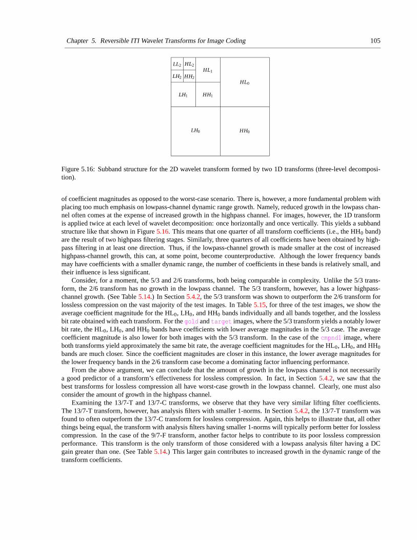
Chapter 5. Reversible ITI Wavelet Transforms for Image Coding 105
HH0LH0
HL0
HH1LH1
HL1HH2LH2
HL2LL2
Figure 5.16: Subband structure for the 2D wavelet transform formed by two 1D transforms (three-level decomposi-tion).
of coefficient magnitudes as opposed to the worst-case scenario. There is, however, a more fundamental problem withplacing too much emphasis on lowpass-channel dynamic range growth. Namely, reduced growth in the lowpass chan-nel often comes at the expense of increased growth in the highpass channel. For images, however, the 1D transformis applied twice at each level of wavelet decomposition: once horizontally and once vertically. This yields a subbandstructure like that shown in Figure 5.16. This means that one quarter of all transform coefficients (i.e., the HH0 band)are the result of two highpass filtering stages. Similarly, three quarters of all coefficients have been obtained by high-pass filtering in at least one direction. Thus, if the lowpass-channel growth is made smaller at the cost of increasedhighpass-channel growth, this can, at some point, become counterproductive. Although the lower frequency bandsmay have coefficients with a smaller dynamic range, the number of coefficients in these bands is relatively small, andtheir influence is less significant.
Consider, for a moment, the 5/3 and 2/6 transforms, both being comparable in complexity. Unlike the 5/3 trans-form, the 2/6 transform has no growth in the lowpass channel. The 5/3 transform, however, has a lower highpass-channel growth. (See Table 5.14.) In Section 5.4.2, the 5/3 transform was shown to outperform the 2/6 transform forlossless compression on the vast majority of the test images. In Table 5.15, for three of the test images, we show theaverage coefficient magnitude for the HL0, LH0, and HH0 bands individually and all bands together, and the losslessbit rate obtained with each transform. For the gold and target images, where the 5/3 transform yields a notably lowerbit rate, the HL0, LH0, and HH0 bands have coefficients with lower average magnitudes in the 5/3 case. The averagecoefficient magnitude is also lower for both images with the 5/3 transform. In the case of the cmpnd1 image, whereboth transforms yield approximately the same bit rate, the average coefficient magnitudes for the HL0, LH0, and HH0
bands are much closer. Since the coefficient magnitudes are closer in this instance, the lower average magnitudes forthe lower frequency bands in the 2/6 transform case become a dominating factor influencing performance.
From the above argument, we can conclude that the amount of growth in the lowpass channel is not necessarilya good predictor of a transform’s effectiveness for lossless compression. In fact, in Section 5.4.2, we saw that thebest transforms for lossless compression all have worst-case growth in the lowpass channel. Clearly, one must alsoconsider the amount of growth in the highpass channel.
Examining the 13/7-T and 13/7-C transforms, we observe that they have very similar lifting filter coefficients.The 13/7-T transform, however, has analysis filters with smaller 1-norms. In Section 5.4.2, the 13/7-T transform wasfound to often outperform the 13/7-C transform for lossless compression. Again, this helps to illustrate that, all otherthings being equal, the transform with analysis filters having smaller 1-norms will typically perform better for losslesscompression. In the case of the 9/7-F transform, another factor helps to contribute to its poor lossless compressionperformance. This transform is the only transform of those considered with a lowpass analysis filter having a DCgain greater than one. (See Table 5.14.) This larger gain contributes to increased growth in the dynamic range of thetransform coefficients.
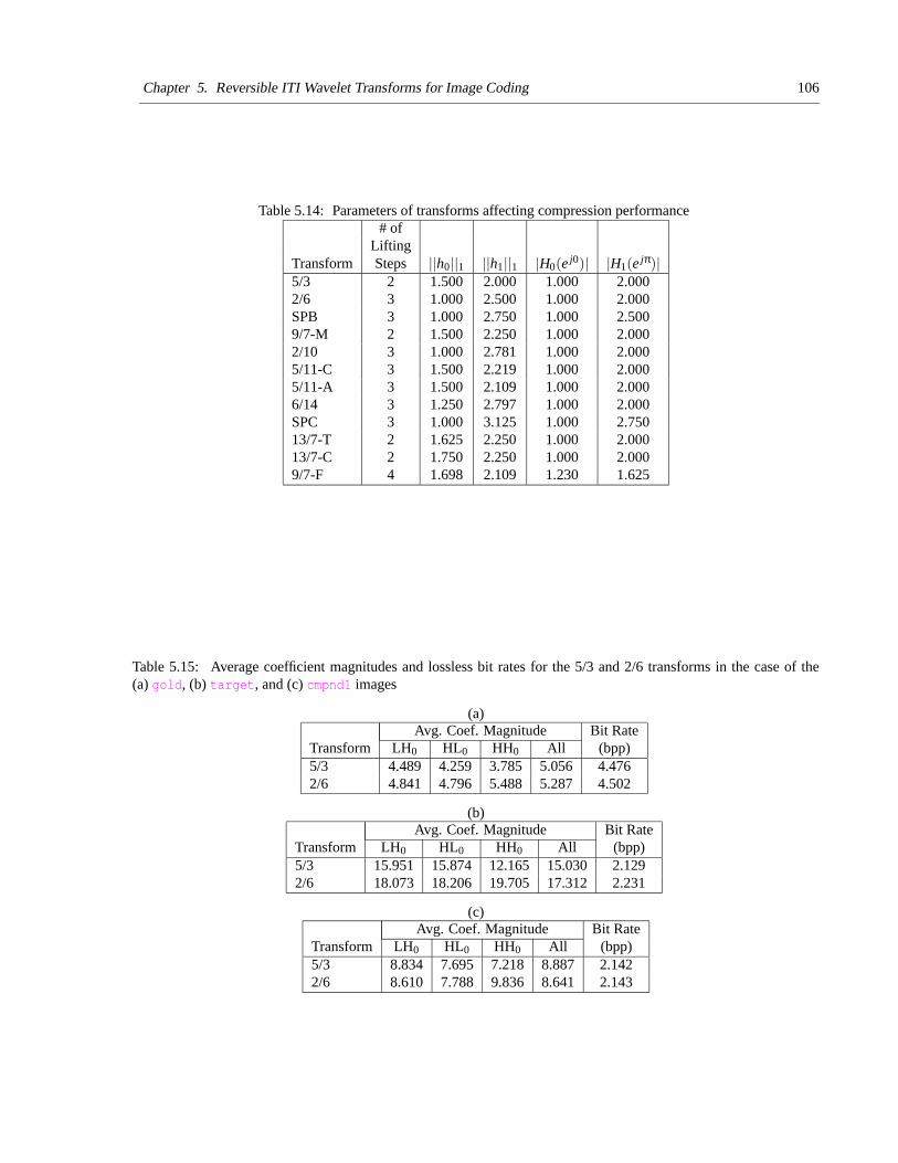
Chapter 5. Reversible ITI Wavelet Transforms for Image Coding 106
Table 5.14: Parameters of transforms affecting compression performance# of
LiftingTransform Steps ||h0||1 ||h1||1 |H0(e j0)| |H1(e jπ)|5/3 2 1.500 2.000 1.000 2.0002/6 3 1.000 2.500 1.000 2.000SPB 3 1.000 2.750 1.000 2.5009/7-M 2 1.500 2.250 1.000 2.0002/10 3 1.000 2.781 1.000 2.0005/11-C 3 1.500 2.219 1.000 2.0005/11-A 3 1.500 2.109 1.000 2.0006/14 3 1.250 2.797 1.000 2.000SPC 3 1.000 3.125 1.000 2.75013/7-T 2 1.625 2.250 1.000 2.00013/7-C 2 1.750 2.250 1.000 2.0009/7-F 4 1.698 2.109 1.230 1.625
Table 5.15: Average coefficient magnitudes and lossless bit rates for the 5/3 and 2/6 transforms in the case of the(a) gold, (b) target, and (c) cmpnd1 images
(a)Avg. Coef. Magnitude Bit Rate
Transform LH0 HL0 HH0 All (bpp)5/3 4.489 4.259 3.785 5.056 4.4762/6 4.841 4.796 5.488 5.287 4.502
(b)Avg. Coef. Magnitude Bit Rate
Transform LH0 HL0 HH0 All (bpp)5/3 15.951 15.874 12.165 15.030 2.1292/6 18.073 18.206 19.705 17.312 2.231
(c)Avg. Coef. Magnitude Bit Rate
Transform LH0 HL0 HH0 All (bpp)5/3 8.834 7.695 7.218 8.887 2.1422/6 8.610 7.788 9.836 8.641 2.143
Chapter 5. Reversible ITI Wavelet Transforms for Image Coding 107
5.6 Summary
Several reversible ITI wavelet transforms have been compared on the basis of their lossy compression performance,lossless compression performance, and computational complexity. For lossless compression, image content is animportant factor influencing transform effectiveness. For smooth images, the 5/11-C, 5/11-A, and 13/7-T transformsare most effective, while the 5/3 transform performs best for images with a greater amount of high frequency content.In the case of lossy compression, both PSNR and subjective performance measures were employed. In terms of PSNRperformance, the 9/7-F, 6/14, 13/7-C, and 13/7-T transforms yield the best results. At the same time, the 9/7-F, 5/3,9/7-M, 5/11-C, 5/11-A, 13/7-T, and 13/7-C transforms achieve the most favorable subjective ratings. Of the transformsconsidered, the 5/3 and 2/6 transforms have the lowest computational complexity while the 9/7-F transform has thehighest. Unfortunately, the 9/7-F transform, although very good for lossy compression, is significantly higher incomplexity than all of the other transforms, and performs poorly for lossless compression.
Obviously, no one transform has superior lossy and lossless compression performance for all classes of imagesin addition to low computational complexity. Therefore, tradeoffs are involved, and the most appropriate choice oftransform depends on the needs of the application at hand. For example, in the case of applications requiring lowcomputational complexity, the 5/3 transform is particularly attractive. It performs reasonably well for both lossy andlossless compression, and has the lowest computational complexity of all of the transforms evaluated.
Reversible ITI and conventional versions of the same transforms were also compared. Using reversible ITI versionsof transforms instead of their conventional counterparts for lossy compression was found to only introduce a slightdegradation in subjective image quality in many cases. When transforms associated with FIR filter banks are employed,the performance penalty is almost negligible. At low bit rates, the difference in PSNR performance is also small.
By examining the performance characteristics of the various reversible ITI wavelet transforms, we were also ableto determine several factors that affect the compression performance of such transforms. By considering these factorsin the future, we can hope to design new and more effective transforms.
Sit down before fact as a little child, be prepared to give up every preconceivednotion, follow humbly wherever and to whatever abysses nature leads, or youshall learn nothing.
—Thomas H. Huxley (1825–1895)
108
Chapter 6
Conclusions and Future Research
Time passes in moments, moments which, rushing past, define the path of a life just as surely asthey lead towards its end. How rarely do we stop to examine that path, to see the reasons why allthings happen, to consider whether the path we take in life is our own making or simply one intowhich we drift with eyes closed? But what if we could stop, pause to take stock of each preciousmoment before it passes? Might we then see the endless forks in the road that have shaped a life?And, seeing those choices, choose another path?
—Dana Scully, The X-Files: All Things
6.1 Conclusions
In this thesis, we have studied reversible ITI wavelet transforms in the context of image coding. In so doing, we havehelped to advance existing knowledge in this area.
In our work, we proposed the GRITIT framework, a single unified framework for reversible ITI wavelet/blocktransforms. This new framework was then used to study several previously developed frameworks and their inter-relationships. In so doing, we were able to gain some interesting new insights into the various frameworks underconsideration. For example, the ORT framework was shown to be a special case of the lifting framework with onlytrivial extensions.
Rounding operators were examined in some detail. Several common rounding operators were characterized interms of their approximation properties and computational complexity, and relationships between these rounding oper-ators were also examined. We showed that, when one considers approximation error and/or computational complexity,the floor, biased floor, and biased ceiling functions are arguably the most practically useful rounding operators of thosestudied.
The GRITIT framework was demonstrated to be useful for the construction of reversible ITI block transforms.The GST, a family of reversible ITI block transforms, was proposed. Then, the GST was studied in detail, leading toa number of interesting insights about transforms in this family. Moreover, the GST framework was used as a meansto derive reduced complexity implementations of the S transform and RCT. A new transform belonging to the GSTfamily, called the MRCT, was introduced, and shown to be practically useful for image coding applications.
Strategies for handling the transformation of arbitrary-length signals in a nonexpansive manner were considered(e.g., periodic extension, symmetric extension, and per-displace-step extension). Two families of symmetry-preservingtransforms (which are compatible with symmetric extension) were introduced and studied. We characterized thetransforms belonging to these families. Some new reversible ITI structures that are useful for constructing symmetry-preserving transforms were also proposed. A simple search-based design technique was explored as means for findingeffective low-complexity transforms in the above-mentioned families, and shown to produce good results.
In the context of image coding, a number of reversible ITI wavelet transforms were compared on the basis of theirlossy compression performance, lossless compression performance, and computational complexity. Of the transformsconsidered, several were found to perform particularly well, with the best choice for a given application depending onthe relative importance of the preceding criteria. Reversible ITI versions of numerous transforms are also compared totheir conventional (i.e., non-reversible real-to-real) counterparts for lossy compression. At low bit rates, reversible ITIand conventional versions of transforms were found to often yield results of comparable quality. Factors affecting thecompression performance of reversible ITI wavelet transforms were also presented, supported by both experimentaldata and theoretical arguments.
Chapter 6. Conclusions and Future Research 109
6.2 Future Research
Although this thesis has made numerous contributions concerning reversible ITI wavelet transforms and their applica-tion to image coding, further work in this area would still be beneficial. Some future research directions are discussedbriefly below.
As described in this thesis, the GRITIT framework can be used to construct (multidimensional) reversible ITIwavelet transforms that are based on nonseparable sampling and filtering operations. This said, however, our workhas focused primarily on the separable case. Since there may be potential benefits offered by transforms based onnonseparable operations, a more thorough consideration of the nonseparable case would certainly be a worthwhileendeavor.
In this thesis, we have focused exclusively on non-adaptive transforms. Obviously, adaptive transforms have thepotential to be much more effective for signals with highly non-stationary statistics. Thus, work in the area of adaptivetransforms could have significant benefits. Obviously, much work could be done in devising good adaptation schemes.Also, clever new techniques for handling the synchronization of the encoder and decoder adaptation algorithms wouldbe quite useful.
In our work, we have considered only reversible ITI transforms that approximate linear wavelet/block transforms.One might want to further explore reversible ITI transforms that are based on operations other than linear filtering (e.g.,median filtering, morphological operators). Such generalizations are easily accommodated by the GRITIT framework,as discussed earlier.
The reversible ITI transform frameworks described in this thesis can be applied to both wavelet and more generalsubband decompositions. In our work, we have not considered the general subband case explicitly. There may bepotential benefits from doing so. Thus, this presents is another possible direction for future research.
6.3 Closing Remarks
This thesis has studied reversible ITI wavelet/block transforms and their application to image coding. By exploitingthe research results presented herein, we can hope to find more effective reversible ITI wavelet/block transforms, andbuild image compression systems with improved coding efficiency. Consequently, the research documented in thisthesis can benefit the many applications in which images are stored and communicated.
In this universe the night was falling; the shadows were lengthening towards aneast that would not know another dawn. But elsewhere the stars were still youngand the light of morning lingered; and along the path he once had followed, Manwould one day go again.
—Arthur C. Clarke, The City and the Stars, 1956
110
Bibliography
[1] M. D. Adams. Reversible wavelet transforms and their application to embedded image compression. M.A.Sc.thesis, Department of Electrical and Computer Engineering, University of Victoria, Victoria, BC, Canada, Jan-uary 1998.
[2] M. D. Adams. The official JasPer home page. http://www.ece.ubc.ca/˜mdadams/jasper, 2000.
[3] M. D. Adams. JasPer software reference manual. ISO/IEC JTC 1/SC 29/WG 1 N 2415, December 2001.
[4] M. D. Adams. The JPEG-2000 still image compression standard. ISO/IEC JTC 1/SC 29/WG 1 N 2412,September 2001. Available online from http://www.ece.ubc.ca/˜mdadams and distributed with the JasPersoftware.
[5] M. D. Adams and A. Antoniou. Reversible EZW-based image compression using best-transform selection andselective partial embedding. IEEE Trans. on Circuits and Systems—II: Analog and Digital Signal Processing,47(10):1119–1122, October 2000.
[6] M. D. Adams, I. Kharitonenko, and F. Kossentini. Report on core experiment CodEff4: Performance evaluationof several reversible integer-to-integer wavelet transforms in the JPEG-2000 verification model (version 2.1).ISO/IEC JTC 1/SC 29/WG 1 N 1015, October 1998.
[7] M. D. Adams and F. Kossentini. Performance evaluation of different decorrelating transforms in the JPEG-2000baseline system. In Proc. of IEEE Symposium on Advances in Digital Filtering and, Signal Processing, pages20–24, Victoria, BC, Canada, June 1998.
[8] M. D. Adams and F. Kossentini. Performance evaluation of different reversible decorrelating transforms in theJPEG-2000 baseline system. ISO/IEC JTC 1/SC 29/WG 1 N 750, March 1998.
[9] M. D. Adams and F. Kossentini. Performance evaluation of several reversible integer-to-integer wavelet trans-forms in the JPEG-2000 baseline system (VM release 0.0). ISO/IEC JTC 1/SC 29/WG 1 N 866, June 1998.
[10] M. D. Adams and F. Kossentini. SBTLIB: A flexible computation engine for subband transforms. ISO/IECJTC 1/SC 29/WG 1 N 867, June 1998.
[11] M. D. Adams and F. Kossentini. Evaluation of reversible integer-to-integer wavelet transforms for image com-pression. In Proc. of IEEE International Conference on Image Processing, volume 3, pages 541–545, Kobe,Japan, October 1999.
[12] M. D. Adams and F. Kossentini. Low-complexity reversible integer-to-integer wavelet transforms for imagecoding. In Proc. of IEEE Pacific Rim Conference on Communications, Computers and Signal Processing,pages 177–180, Victoria, BC, Canada, August 1999.
[13] M. D. Adams and F. Kossentini. Performance evaluation of reversible integer-to-integer wavelet transforms forimage compression. In Proc. of IEEE Data Compression Conference, page 514, Snowbird, UT, USA, March1999.
[14] M. D. Adams and F. Kossentini. JasPer: A software-based JPEG-2000 codec implementation. In Proc. of IEEEInternational Conference on Image Processing, volume 2, pages 53–56, Vancouver, BC, Canada, October 2000.
[15] M. D. Adams and F. Kossentini. On the relationship between the overlapping rounding transform and liftingframeworks for reversible subband transforms. IEEE Trans. on Signal Processing, 48(1):261–266, January2000.
Bibliography 111
[16] M. D. Adams and F. Kossentini. Reversible integer-to-integer wavelet transforms for image compression:Performance evaluation and analysis. IEEE Trans. on Image Processing, 9(6):1010–1024, June 2000.
[17] M. D. Adams and F. Kossentini. Generalized S transform. In Proc. of IEEE International Conference onAcoustics, Speech, and Signal Processing, volume 3, pages 1749–1752, Salt Lake City, UT, USA, May 2001.
[18] M. D. Adams, F. Kossentini, and R. Ward. Generalized S transform. IEEE Trans. on Signal Processing, 2002.To appear.
[19] M. D. Adams and R. Ward. Wavelet transforms in the JPEG-2000 standard. In Proc. of IEEE Pacific RimConference on Communications, Computers and Signal Processing, volume 1, pages 160–163, Victoria, BC,Canada, 2001.
[20] M. D. Adams and R. Ward. Symmetry-preserving reversible integer-to-integer wavelet transforms. In Proc.of IEEE International Conference on Acoustics, Speech, and Signal Processing, volume 3, pages 2509–2512,Orlando, FL, USA, May 2002.
[21] M. D. Adams and R. Ward. Symmetry-preserving reversible integer-to-integer wavelet transforms. Submittedto IEEE Trans. on Signal Processing, January 2002.
[22] M. D. Adams and R. Ward. Two families of symmetry-preserving reversible integer-to-integer wavelet trans-forms. In Proc. of IEEE International Symposium on Circuits and Systems, volume 2, pages 600–603, Scotts-dale, AZ, USA, May 2002.
[23] R. Ansari, E. Ceran, and N. Memon. Near-lossless image compression techniques. In Proc. of SPIE: VisualCommunications and Image Processing, volume 3309, pages 731–742, January 1998.
[24] M. Antonini, M. Barlaud, P. Mathieu, and I. Daubechies. Image coding using wavelet transform. IEEE Trans.on Image Processing, 1(2):205–220, April 1992.
[25] J. Askelof, M. Larsson Carlander, and C. Christopoulos. Region of interest coding in JPEG 2000. SignalProcessing: Image Communication, 17(1):105–111, January 2002.
[26] E. Atsumi and N. Farvardin. Lossy/lossless region-of-interest image coding based on set partitioning in hierar-chical trees. In Proc. of IEEE International Conference on Image Processing, volume 1, pages 87–91, Chicago,IL, USA, October 1998.
[27] B. Berthelot, E. Majani, and P. Onno. Transform core experiment: Compare the SNR performance of variousreversible integer wavelet transforms. ISO/IEC JTC 1/SC 29/WG 1 N 902, June 1998.
[28] H. Blume and A. Fand. Reversible and irreversible image data compression using the S-transform and Lempel-Ziv coding. In Proc. of SPIE, volume 1091, pages 2–18, Newport Beach, CA, USA, January 1989.
[29] M. Boliek, M. J. Gormish, E. L. Schwartz, and A. Keith. Next generation image compression and manipulationusing CREW. In Proc. of IEEE International Conference on Image Processing, volume 3, pages 567–570,Santa Barbara, CA, USA, October 1997.
[30] A. D. Booth. A signed binary multiplication technique. Quarterly Journal of Mechanics and Applied Mathe-matics, 4:236–240, 1951.
[31] C. Brislawn, S. Mniszewski, M. Pal, A. Percus, B. Wohlberg, T. Acharya, P.-S. Tsai, and M. Lepley. Even-lengthfilter bank option. ISO/IEC JTC 1/SC 29/WG 1 N 2209, July 2001.
[32] C. Brislawn and B. Wohlberg. Boundary extensions and reversible implementation for half-sample symmetricfilter banks. ISO/IEC JTC 1/SC 29/WG 1 N 2119, March 2001.
[33] C. M. Brislawn. Preservation of subband symmetry in multirate signal coding. IEEE Trans. on Signal Process-ing, 43(12):3046–3050, December 1995.
[34] C. M. Brislawn. Classification of nonexpansive symmetric extension transforms for multirate filter banks.Applied and Computational Harmonic Analysis, 3(4):337–357, October 1996.
Bibliography 112
[35] C. M. Brislawn, J. N. Bradley, R. J. Onyshczak, and T. Hopper. The FBI compression standard for digitizedfingerprint images. Preprint, 1996.
[36] F. A. M. L. Bruekers and A. W. M. van den Enden. New networks for perfect inversion and perfect reconstruc-tion. IEEE Journal on Selected Areas in Communications, 10(1):130–137, January 1992.
[37] C. S. Burrus, R. A. Gopinath, and H. Guo. Introduction to Wavelets and Wavelet Transforms: A Primer. PrenticeHall, Upper Saddle River, NJ, USA, 1998.
[38] A. R. Calderbank, I. Daubechies, W. Sweldens, and B.-L. Yeo. Wavelet transforms that map integers to integers.Technical report, Department of Mathematics, Princeton University, August 1996.
[39] A. R. Calderbank, I. Daubechies, W. Sweldens, and B.-L. Yeo. Lossless image compression using integer tointeger wavelet transforms. In Proc. of IEEE International Conference on Image Processing, volume 1, pages596–599, Santa Barbara, CA, USA, October 1997.
[40] A. R. Calderbank, I. Daubechies, W. Sweldens, and B.-L. Yeo. Wavelet transforms that map integers to integers.Applied and Computational Harmonic Analysis, 5(3):332–369, July 1998.
[41] B. Carpentieri, M. J. Weinberger, and G. Seroussi. Lossless compression of continuous-tone images. Proc. ofIEEE, 88(11):1797–1809, November 2000.
[42] J. J. F. Cavanagh. Digital Computer Arithmetic: Design and Implementation. McGraw-Hill, New York, 1984.
[43] H. Cha and L. F. Chaparro. Adaptive morphological representation of signals: polynomial and wavelet methods.Multidimensional Systems and Signal Processing, 8(3):249–271, July 1997.
[44] H. Chao, P. Fisher, and Z. Hua. An approach to integer wavelet transforms for lossless for image compression.In Proc. of International Symposium on Computational Mathematics, pages 19–38, Guangzhou, China, August1997.
[45] T. Chen and P. P. Vaidyanathan. Multidimensional multirate filters and filter banks derived from one dimensionalfilters. IEEE Trans. on Signal Processing, 41(5):1749–1765, May 1993.
[46] C. Christopoulos, J. Askelof, and M. Larsson. Efficient methods for encoding regions of interest in the upcomingJPEG 2000 still image coding standard. IEEE Signal Processing Letters, 7(9):247–249, September 2000.
[47] C. Christopoulos, A. Skodras, and T. Ebrahimi. The JPEG 2000 still image coding system: An overview. IEEETrans. on Consumer Electronics, 46(4):1103–1127, November 2000.
[48] T. Cooklev, A. Nishihara, T. Yoshida, and M. Sablatash. Multidimensional two-channel linear phase FIR filterbanks and wavelet bases with vanishing moments. Multidimensional Systems and Signal Processing, 9(1):39–76, January 1998.
[49] I. Daubechies and W. Sweldens. Factoring wavelet transforms into lifting steps. Journal of Fourier Analysisand Applications, 4:247–269, 1998.
[50] S. Dewitte and J. Cornelis. Lossless integer wavelet transform. IEEE Signal Processing Letters, 4(6):158–160,June 1997.
[51] S. Dewitte, P. De Muynck, A. Munteanu, and J. Cornelis. Lossless image subband coding with an integerwavelet transform. In Proc. of International Conference on Digital Signal Processing, volume 2, pages 555–557, Santorini, Greece, July 1997.
[52] E. Dubois. The sampling and reconstruction of time-varying imagery with application in video systems. Proc.of IEEE, 73(4):502–522, April 1985.
[53] D. E. Dudgeon and R. M. Mersereau. Multidimensional Digital Signal Processing. Prentice-Hall, EnglewoodCliffs, NJ, USA, 1984.
Bibliography 113
[54] O. Egger, W. Li, and M. Kunt. High compression image coding using an adaptive morphological subbanddecomposition. Proc. of IEEE, 83(2):272–287, February 1995.
[55] D. Le Gall and A. Tabatabai. Sub-band coding of digital images using symmetric short kernel filters andarithmetic coding techniques. In Proc. of IEEE International Conference on Acoustics, Speech, and SignalProcessing, volume 2, pages 761–764, New York, NY, USA, April 1988.
[56] R. S. Garfinkel and G. L. Nemhauser. Integer Programming. John Wiley and Sons, Toronto, ON, Canada, 1972.
[57] O. N. Gerek and A. E. Cetin. Linear/nonlinear adaptive polyphase subband decomposition structures for im-age compression. In Proc. of IEEE International Conference on Acoustics, Speech, and Signal Processing,volume 3, pages 1345–1348, Seattle, WA, USA, May 1998.
[58] O. N. Gerek and A. E. Cetin. Adaptive polyphase subband decomposition structures for image compression.IEEE Trans. on Image Processing, 9(10):1649–1660, October 2000.
[59] M. J. Gormish, E. L. Schwartz, A. F. Keith, M. P. Boliek, and A. Zandi. Lossless and nearly lossless compressionof high-quality images. In Proc. of SPIE, volume 3025, pages 62–70, San Jose, CA, USA, March 1997.
[60] J. Goutsias and H. J. A. M. Heijmans. Nonlinear multiresolution signal decomposition schemes—part i: Mor-phological pyramids. IEEE Trans. on Image Processing, 9(11):1862–1876, November 2000.
[61] Independent JPEG Group. JPEG library (version 6b). Available online from http://www.ijg.org, 2000.
[62] A. Haar. Zur theorie der orthogonalen funktionen-systeme. Math. Annal., 69:331–371, 1910.
[63] P. Hao and Q. Shi. Matrix factorizations for reversible integer mapping. IEEE Trans. on Signal Processing,49(10):2314–2324, October 2001.
[64] R. He, J. Bai, and D. Ye. Properties for perfect reconstruction using multirate linear phase two-dimensionalnonseparable filter banks and its implementation. Optical Engineering, 37(8):2363–2375, August 1998.
[65] H. J. A. M. Heijmans and J. Goutsias. Nonlinear multiresolution signal decomposition schemes—part ii: Mor-phological wavelets. IEEE Trans. on Image Processing, 9(11):1897–1913, November 2000.
[66] J. S. Houchin and D. W. Singer. File format technology in JPEG 2000 enables flexible use of still and motionsequences. Signal Processing: Image Communication, 17(1):131–144, January 2002.
[67] ISO/IEC call for contributions, JPEG 2000. ISO/IEC JTC 1/SC 29/WG 1 N505, March 1997.
[68] JPEG-2000 test images. ISO/IEC JTC 1/SC 29/WG 1 N 545, July 1997.
[69] ISO/IEC 10918-1:1994, Information technology—Digital compression and coding of continuous-tone still im-ages: Requirements and guidelines, 1994.
[70] ISO/IEC 14492: Information technology—Lossy/lossless coding of bi-level images, 2001.
[71] ISO/IEC 14495-1: Lossless and near-lossless compression of continuous-tone still images: Baseline, 2000.
[72] ISO/IEC 15444-1: Information technology—JPEG 2000 image coding system—Part 1: Core coding system,2000.
[73] ISO/IEC 15444-2: Information technology—JPEG 2000 image coding system—Part 2: Extensions, 2002.
[74] ISO/IEC 15444-3: Information technology—JPEG 2000 image coding system—Part 3: Motion JPEG 2000,2002.
[75] ISO/IEC 15444-4: Information technology—JPEG 2000 image coding system—Part 4: Compliance testing,2002.
[76] ISO/IEC 15444-5: Information technology—JPEG 2000 image coding system—Part 5: Reference software,2002.
Bibliography 114
[77] N. S. Jayant and P. Noll. Digital Coding of Waveforms: Principals and Applications to Speech and Video.Prentice-Hall, Englewood Cliffs, NJ, USA, 1984.
[78] H.-Y. Jung and R. Prost. Rounding transform based approach for lossless subband coding. In Proc. of IEEEInternational Conference on Image Processing, volume 2, pages 274–277, Santa Barbara, CA, USA, October1997.
[79] H.-Y. Jung and R. Prost. Lossless subband coding system based on rounding transform. IEEE Trans. on SignalProcessing, 46(9):2535–2540, September 1998.
[80] H.-Y. Jung and R. Prost. Multi-port filtering system for lossless image compression. In Proc. of IEEE Interna-tional Conference on Image Processing, volume 3, pages 861–865, Chicago, IL, USA, October 1998.
[81] A. A. C. Kalker and I. A. Shah. Ladder structures for multidimensional linear phase perfect reconstruction filterbanks and wavelets. In Proc. of SPIE, volume 1818, pages 12–20, Boston, MA, USA, November 1992.
[82] T. A. C. M. Kalker and I. A. Shah. On ladder structures and linear phase conditions for multidimensionalbi-orthogonal filter banks. Preprint, June 1993.
[83] G. Karlsson and M. Vetterli. Theory of two dimensional multirate filter banks. IEEE Trans. on Acoustics,Speech, and Signal Proceesing, 38:925–937, June 1990.
[84] J. H. Kasner, M. W. Marcellin, and B. R. Hunt. Universal trellis coded quantization. IEEE Trans. on ImageProcessing, 8(12):1677–1687, December 1999.
[85] H. Kim and C. C. Li. A fast reversible wavelet image compressor. In Proc. of SPIE, volume 2825, pages929–940, 1996.
[86] H. Kim and C. C. Li. Lossless and lossy image compression using biorthogonal wavelet transforms withmultiplierless operations. IEEE Trans. on Circuits and Systems, 45(8):1113–1118, August 1998.
[87] K. Komatsu and K. Sezaki. Reversible subband coding of images. In Proc. of SPIE, volume 2501, pages676–684, 1995.
[88] K. Komatsu and K. Sezaki. Design of lossless block transforms and filter banks for image coding. IEICE Trans.Fundamentals, E82-A(8):1656–1664, August 1999.
[89] K. Komatsu and K. Sezaki. Lossless filter banks based on two point transform and interpolative prediction. InProc. of IEEE International Conference on Acoustics, Speech, and Signal Processing, volume 3, pages 1469–1472, Phoenix, AZ, USA, March 1999.
[90] J. Kovacevic and W. Sweldens. Wavelet families of increasing order in arbitrary dimensions. IEEE Trans. onImage Processing, 9(3):480–496, March 2000.
[91] J. Kovacevic and M. Vetterli. Nonseparable multidimensional perfect reconstruction filter banks and waveletbases for Rn. IEEE Trans. on Information Theory, 38(2):533–555, March 1992.
[92] A. S. Lewis and G. Knowles. Image compression using the 2-D wavelet transform. IEEE Trans. on ImageProcessing, 1(2):244–250, April 1992.
[93] X. Li, B. Tao, and M. T. Orchard. On implementing transforms from integers to integers. In Proc. of IEEEInternational Conference on Image Processing, volume 3, pages 881–885, Chicago, IL, USA, October 1998.
[94] J. S. Lim. Two-Dimensional Signal and Image Processing. Prentice Hall, Englewood Cliffs, NJ, USA, 1990.
[95] Y.-P. Lin and P. P. Vaidyanathan. Theory and design of two-dimensional filter banks: A review. Multidimen-sional Systems and Signal Processing, 7(3-4):263–330, July 1996.
[96] P. Lux. A novel set of closed orthogonal functions for picture coding. Archiv fur Elektronik und Uebertragung-stechnik, 31(7):267–274, July 1977.
Bibliography 115
[97] M. W. Marcellin, M. A. Lepley, A. Bilgin, T. J. Flohr, T. T. Chinen, and J. H. Kasner. An overview of quanziationin JPEG 2000. Signal Processing: Image Communication, 17(1):73–84, January 2002.
[98] T. G. Marshall. Zero-phase filter bank and wavelet code r matrices: Properties, triangular decompositions, anda fast algorithm. Multidimensional Systems and Signal Processing, 8:71–88, 1997.
[99] S. A. Martucci and R. M. Mersereau. The symmetric convolution approach to the nonexpansive implementationof FIR filter banks for images. In Proc. of IEEE International Conference on Acoustics, Speech, and SignalProcessing, volume 5, pages 65–68, Minneapolis, MN, USA, April 1993.
[100] N. Memon, X. Wu, and B.-L. Yeo. Improved techniques for lossless image compression with reversible integerwavelet transforms. In Proc. of IEEE International Conference on Image Processing, volume 3, pages 891–895,Chicago, IL, USA, October 1998.
[101] A. Munteanu, J. Cornelis, P. De Muynck, and P. Cristea. Wavelet lossless compression of coronary angiographicimages. In Computers in Cardiology, volume 24, pages 183–186, September 1997.
[102] D. Nister and C. Christopoulos. Lossless region of interest with a naturally progressive still image codingalgorithm. In Proc. of IEEE International Conference on Image Processing, volume 3, pages 856–860, Chicago,IL, USA, October 1998.
[103] University of British Columbia. JPEG-LS codec software. Available online from http://spmg.ece.ubc.ca,2000. version 2.2.
[104] S. Oraintara, Y. J. Chen, and T. Q. Nguyen. Integer fast Fourier transform. IEEE Trans. on Signal Processing,50(3):607–618, 2002.
[105] H. Park, T. Kalker, and M. Vetterli. Grobner bases and multidimensional FIR multirate systems. Multidimen-sional Systems and Signal Processing, 8(1–2):11–30, 1997.
[106] H. Park and C. Woodburn. An algorithmic proof of Suslin’s stability theorem for polynomial rings. Journal ofAlgebra, 178(1):277–298, November 1995.
[107] W. B. Pennebaker and J. L. Mitchell. JPEG: Still Image Data Compression Standard. Kluwer Academic, NewYork, NY, USA, 1992.
[108] M. Rabbani and P. W. Jones. Digital Image Compression Techniques. SPIE Optical Engineering Press, Belling-ham, WA, USA, 1991.
[109] M. Rabbani and R. Joshi. An overview of the JPEG2000 still image compression standard. Signal Processing:Image Communication, 17(1):3–48, January 2002.
[110] S. Ranganath and H. Blume. Hierarchical image decomposition and filtering using the s-transform (radiologicalimages). In Proc. of SPIE, volume 914, pages 799–814, Newport Beach, CA, USA, January 1988.
[111] D. W. Redmill and D. R. Bull. Multiplier-free linear phase filter banks for image and video compression. InProc. of SPIE, volume 3309, pages 634–644, San Jose, CA, USA, January 1998.
[112] SAIC and University of Arizona. JPEG-2000 VM 0 software. ISO/IEC JTC 1/SC 29/WG 1 N 840, May 1998.
[113] SAIC and University of Arizona. JPEG-2000 VM software (version 7.1). ISO/IEC JTC 1/SC 29/WG 1 N 1691,April 2000.
[114] A. Said and W. A. Pearlman. An image multiresolution representation for lossless and lossy compression. IEEETrans. on Image Processing, 5(9):1303–1310, September 1996.
[115] A. Said and W. A. Pearlman. A new fast and efficient image codec based on set partitioning in hierarchicaltrees. IEEE Trans. on Circuits and Systems for Video Technology, 6(3):243–250, June 1996.
[116] D. Santa-Cruz, R. Grosbois, and T. Ebrahimi. JPEG 2000 performance evaluation and assessment. SignalProcessing: Image Communication, 17(1):113–130, January 2002.
Bibliography 116
[117] I. Shah and A. Kalker. Theory and design of multidimensional QMF sub-band filters from 1-D filters and poly-nomials using transforms. IEE Proceedings I: Communications, Speech and Vision, 140(1):67–71, February1993.
[118] I. A. Shah, O. Akiwumi-Assani, and B. Johnson. A chip set for lossless image compression. IEEE Journal ofSolid-State Circuits, 26(3):237–244, March 1991.
[119] J. M. Shapiro. Embedded image coding using zerotrees of wavelet coefficients. IEEE Trans. on Signal Process-ing, 41(12):3445–3462, December 1993.
[120] F. Sheng, A. Bilgin, P. J. Sementilli, and M. W. Marcellin. Lossy and lossless image compression using re-versible integer wavelet transforms. In Proc. of IEEE International Conference on Image Processing, volume 3,pages 876–880, Chicago, IL, USA, October 1998.
[121] J. E. Shockley. Introduction to Number Theory. Holt, Rinehart, and Winston, Toronto, ON, Canada, 1967.
[122] M. J. T. Smith and S. L. Eddins. Subband coding of images with octave band tree structures. In Proc. of IEEEInternational Conference on Acoustics, Speech, and Signal Processing, pages 1382–1385, Dallas, TX, USA,1987.
[123] M. J. T. Smith and S. L. Eddins. Analysis/synthesis techniques for subband image coding. IEEE Trans. onAcoustics, Speech, and Signal Proceesing, 38(8):1446–1456, August 1990.
[124] SPIHT home page. Available online from http://www.cipr.rpi.edu/research/SPIHT, 2000.
[125] G. Strang and T. Nguyen. Wavelets and Filter Banks. Wellesley-Cambridge Press, Wellesley, MA, USA, 1996.
[126] N. Strobel, S. K. Mitra, and B. S. Manjunath. Progressive-resolution transmission and lossless compressionof color images for digital image libraries. In Proc. of International Conference on Digital Signal Processing,volume 1, pages 435–438, Santorini, Greece, July 1997.
[127] N. Strobel, S. K. Mitra, and B. S. Manjunath. Reversible wavelet and spectral transforms for lossless com-pression of color images. In Proc. of IEEE International Conference on Image Processing, volume 3, pages896–900, Chicago, IL, USA, October 1998.
[128] A. Suslin. On the structure of the special linear group over polynomial rings. Mathematics of the USSR Izvestija,11:221–238, 1977.
[129] W. Sweldens. The lifting scheme: A new philosophy in biorthogonal wavelet constructions. In Proc. of SPIE,volume 2569, pages 68–79, San Diego, CA, USA, September 1995.
[130] W. Sweldens. The lifting scheme: A custom-design construction of biorthogonal wavelets. Applied and Com-putational Harmonic Analysis, 3(2):186–200, 1996.
[131] W. Sweldens. The lifting scheme: A construction of second generation wavelets. SIAM Journal of MathematicalAnalysis, 29(2):511–546, March 1998.
[132] D. Taubman. High performance scalable image compression with EBCOT. In Proc. of IEEE InternationalConference on Image Processing, volume 3, pages 344–348, Kobe, Japan, 1999.
[133] D. Taubman. High performance scalable image compression with EBCOT. IEEE Trans. on Image Processing,9(7):1158–1170, July 2000.
[134] D. Taubman, E. Ordentlich, M. Weinberger, and G. Seroussi. Embedded block coding in JPEG 2000. SignalProcessing: Image Communication, 17(1):49–72, January 2002.
[135] D. S. Taubman and M. W. Marcellin. JPEG2000: Image Compression Fundamentals, Standards and Practice.Kluwer Academic, Boston, MA, USA, 2002.
[136] D. B. H. Tay and N. G. Kingbury. Flexible design of multidimensional perfect reconstruction FIR two-bandfilters using transformation of variables. IEEE Trans. on Image Processing, 2(4):466–480, October 1993.
Bibliography 117
[137] L. Tolhuizen, H. Hollmann, and T. A. C. M. Kalker. On the realizability of biorthogonal m-dimensional two-band filter banks. IEEE Trans. on Signal Processing, 43(3):640–648, March 1995.
[138] P. P. Vaidyanathan. Fundamentals of multidimensional multirate digital signal processing. Sadhana, 15(3):157–176, November 1990.
[139] P. P. Vaidyanathan. Multirate digital filters, filter banks, polyphase networks, and applications: a tutorial. Proc.of IEEE, 78(1):56–93, January 1990.
[140] P. P. Vaidyanathan. Multirate Systems and Filter Banks. Prentice-Hall, Englewood Cliffs, NJ, USA, 1993.
[141] M. Vetterli and J. Kovacevic. Wavelets and Subband Coding. Prentice-Hall, Englewood Cliffs, NJ, USA, 1995.
[142] J. D. Villasenor, B. Belzer, and J. Liao. Wavelet filter evaluation for image compression. IEEE Trans. on ImageProcessing, 4(8):1053–1060, August 1995.
[143] E. Viscito and J. P. Allebach. The analysis and design of multidimensional FIR perfect reconstruction filterbanks for arbitrary sampling lattices. IEEE Trans. on Circuits and Systems, 38(1):29–41, January 1991.
[144] G. K. Wallace. The JPEG still picture compression standard. Communications of the ACM, 34(4):30–44, April1991.
[145] M. J. Weinberger, G. Seroussi, and G. Sapiro. The LOCO-I lossless image compression algorithm: Principlesand standarization into JPEG-LS. IEEE Trans. on Image Processing, 9(8):1309–1324, August 2000.
[146] T. Wendler. Verfahren fur die hierarchische Codierung von Einzelbildern in medizinischen Bildinformation-ssystemen. Dr. Ing. thesis, Rheinisch-Westfalische Technische Hochschule Aachen, Germany, 1987.
[147] I. H. Witten, R. M. Neal, and J. G. Cleary. Arithmetic coding for data compression. Communications of theACM, 30(6):520–540, 1987.
[148] A. Zandi, J. D. Allen, E. L. Schwartz, and M. Boliek. CREW: Compression with reversible embedded wavelets.In Proc. of IEEE Data Compression Conference, pages 212–221, Snowbird, UT, USA, March 1995.
[149] W. Zeng, S. Daly, and S. Lei. An overview of the visual optimization tools in JPEG 2000. Signal Processing:Image Communication, 17(1):85–104, January 2002.
[150] Y. Zeng, L. Cheng, G. Bi, and A. C. Kot. Integer DCTs and fast algorithms. IEEE Trans. on Signal Processing,49(11):2774–2782, 2001.
I am enough of an artist to draw freely upon my imagination. Imagination ismore important than knowledge. Knowledge is limited. Imagination encirclesthe world.
—Albert Einstein (1879–1955)
118
Appendix A
JPEG 2000: An International Standard forStill Image Compression
Many that live deserve death. And some that die deserve life. Can you give it to them? Then do notbe too eager to deal out death in judgement. For even the very wise cannot see all ends.
—J. R. R. Tolkein, The Fellowship of the Ring, 1954
Overview
The JPEG-2000 image compression standard is introduced, and the JPEG-2000 Part-1 codec is described, analyzed,and evaluated. The JasPer software is also discussed briefly.
A.1 Introduction
Digital imagery is pervasive in our world today. Consequently, standards for the efficient representation and inter-change of digital images are essential. To date, some of the most successful still image compression standards haveresulted from the ongoing work of the Joint Photographic Experts Group (JPEG). This group operates under the aus-pices of Joint Technical Committee 1, Subcommittee 29, Working Group 1 (JTC 1/SC 29/WG 1), a collaborativeeffort between the International Organization for Standardization (ISO) and International Telecommunication UnionStandardization Sector (ITU-T). Both the JPEG [69,144,107] and JPEG-LS [71,145,41] standards were born from thework of the JPEG committee. For the last few years, the JPEG committee has been working towards the establishmentof a new standard known as JPEG 2000 (i.e., ISO/IEC 15444). The fruits of these labors are now coming to bear, asJPEG-2000 Part 1 (i.e., ISO/IEC 15444-1 [72]) has recently been approved as a new international standard.
In this appendix, we provide a detailed technical description of the JPEG-2000 Part-1 codec, in addition to a briefoverview of the JPEG-2000 standard. (Some of the material in this appendix has also appeared in [4, 14].) Thisexposition is intended to serve as a reader-friendly starting point for those interested in learning about JPEG 2000.Although many details are included in our presentation, some details are necessarily omitted. The reader should,therefore, refer to the standard [72] before attempting an implementation. The JPEG-2000 codec realization in theJasPer software [2,14,3] may also serve as a practical guide for implementors. (See Section A.6 for more informationabout JasPer.) The reader may also find [135,109,47] to be useful sources of information on the JPEG-2000 standard.
The remainder of this appendix is structured as follows. Section A.2 begins with a overview of the JPEG-2000standard. This is followed, in Section A.3, by a detailed description of the JPEG-2000 Part-1 codec. In Section A.4, thecodec is evaluated. The complexity of its various components is analyzed, and its performance is compared to codecsfrom other existing standards. Finally, we conclude this appendix with a brief summary of our results and some closingremarks in Section A.5. Throughout our presentation, a basic understanding of image coding is assumed.
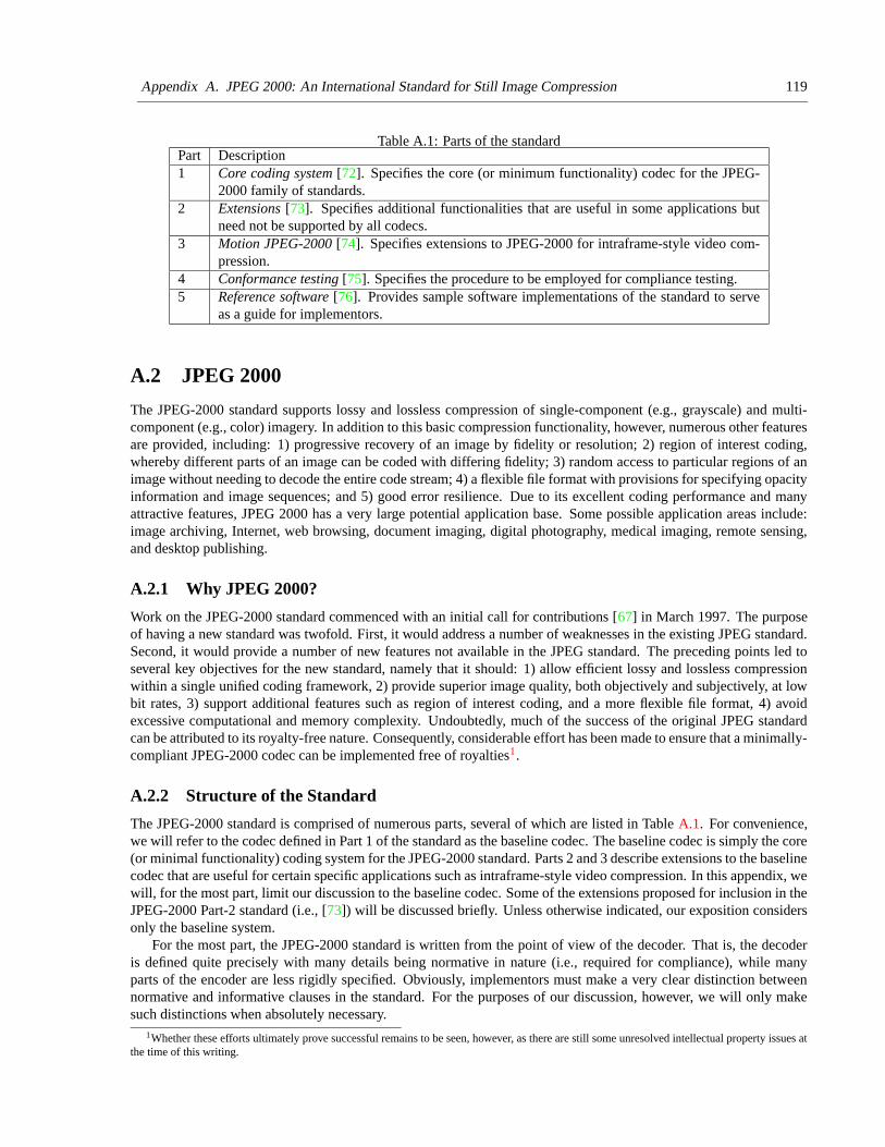
Appendix A. JPEG 2000: An International Standard for Still Image Compression 119
Table A.1: Parts of the standardPart Description1 Core coding system [72]. Specifies the core (or minimum functionality) codec for the JPEG-
2000 family of standards.2 Extensions [73]. Specifies additional functionalities that are useful in some applications but
need not be supported by all codecs.3 Motion JPEG-2000 [74]. Specifies extensions to JPEG-2000 for intraframe-style video com-
pression.4 Conformance testing [75]. Specifies the procedure to be employed for compliance testing.5 Reference software [76]. Provides sample software implementations of the standard to serve
as a guide for implementors.
A.2 JPEG 2000
The JPEG-2000 standard supports lossy and lossless compression of single-component (e.g., grayscale) and multi-component (e.g., color) imagery. In addition to this basic compression functionality, however, numerous other featuresare provided, including: 1) progressive recovery of an image by fidelity or resolution; 2) region of interest coding,whereby different parts of an image can be coded with differing fidelity; 3) random access to particular regions of animage without needing to decode the entire code stream; 4) a flexible file format with provisions for specifying opacityinformation and image sequences; and 5) good error resilience. Due to its excellent coding performance and manyattractive features, JPEG 2000 has a very large potential application base. Some possible application areas include:image archiving, Internet, web browsing, document imaging, digital photography, medical imaging, remote sensing,and desktop publishing.
A.2.1 Why JPEG 2000?
Work on the JPEG-2000 standard commenced with an initial call for contributions [67] in March 1997. The purposeof having a new standard was twofold. First, it would address a number of weaknesses in the existing JPEG standard.Second, it would provide a number of new features not available in the JPEG standard. The preceding points led toseveral key objectives for the new standard, namely that it should: 1) allow efficient lossy and lossless compressionwithin a single unified coding framework, 2) provide superior image quality, both objectively and subjectively, at lowbit rates, 3) support additional features such as region of interest coding, and a more flexible file format, 4) avoidexcessive computational and memory complexity. Undoubtedly, much of the success of the original JPEG standardcan be attributed to its royalty-free nature. Consequently, considerable effort has been made to ensure that a minimally-compliant JPEG-2000 codec can be implemented free of royalties1.
A.2.2 Structure of the Standard
The JPEG-2000 standard is comprised of numerous parts, several of which are listed in Table A.1. For convenience,we will refer to the codec defined in Part 1 of the standard as the baseline codec. The baseline codec is simply the core(or minimal functionality) coding system for the JPEG-2000 standard. Parts 2 and 3 describe extensions to the baselinecodec that are useful for certain specific applications such as intraframe-style video compression. In this appendix, wewill, for the most part, limit our discussion to the baseline codec. Some of the extensions proposed for inclusion in theJPEG-2000 Part-2 standard (i.e., [73]) will be discussed briefly. Unless otherwise indicated, our exposition considersonly the baseline system.
For the most part, the JPEG-2000 standard is written from the point of view of the decoder. That is, the decoderis defined quite precisely with many details being normative in nature (i.e., required for compliance), while manyparts of the encoder are less rigidly specified. Obviously, implementors must make a very clear distinction betweennormative and informative clauses in the standard. For the purposes of our discussion, however, we will only makesuch distinctions when absolutely necessary.
1Whether these efforts ultimately prove successful remains to be seen, however, as there are still some unresolved intellectual property issues atthe time of this writing.
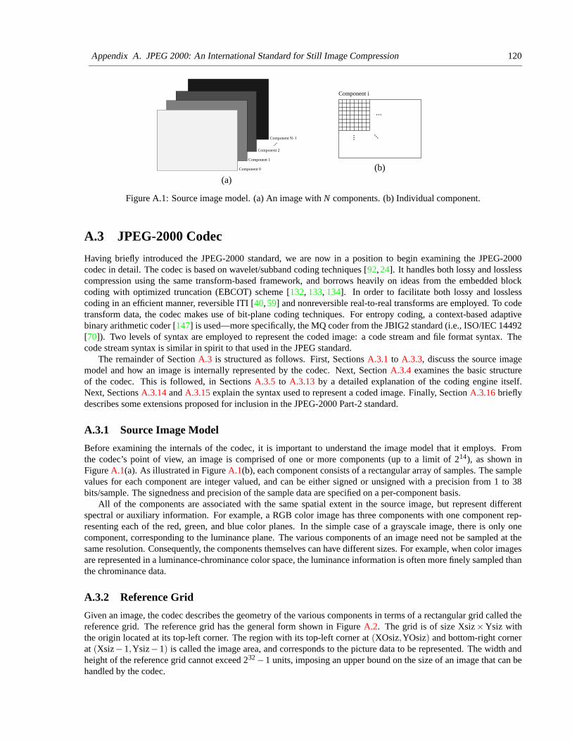
Appendix A. JPEG 2000: An International Standard for Still Image Compression 120
Component 1
Component 2...
Component 0
Component N−1
(a)
Component i
...
...
...
(b)
Figure A.1: Source image model. (a) An image with N components. (b) Individual component.
A.3 JPEG-2000 Codec
Having briefly introduced the JPEG-2000 standard, we are now in a position to begin examining the JPEG-2000codec in detail. The codec is based on wavelet/subband coding techniques [92, 24]. It handles both lossy and losslesscompression using the same transform-based framework, and borrows heavily on ideas from the embedded blockcoding with optimized truncation (EBCOT) scheme [132, 133, 134]. In order to facilitate both lossy and losslesscoding in an efficient manner, reversible ITI [40, 59] and nonreversible real-to-real transforms are employed. To codetransform data, the codec makes use of bit-plane coding techniques. For entropy coding, a context-based adaptivebinary arithmetic coder [147] is used—more specifically, the MQ coder from the JBIG2 standard (i.e., ISO/IEC 14492[70]). Two levels of syntax are employed to represent the coded image: a code stream and file format syntax. Thecode stream syntax is similar in spirit to that used in the JPEG standard.
The remainder of Section A.3 is structured as follows. First, Sections A.3.1 to A.3.3, discuss the source imagemodel and how an image is internally represented by the codec. Next, Section A.3.4 examines the basic structureof the codec. This is followed, in Sections A.3.5 to A.3.13 by a detailed explanation of the coding engine itself.Next, Sections A.3.14 and A.3.15 explain the syntax used to represent a coded image. Finally, Section A.3.16 brieflydescribes some extensions proposed for inclusion in the JPEG-2000 Part-2 standard.
A.3.1 Source Image Model
Before examining the internals of the codec, it is important to understand the image model that it employs. Fromthe codec’s point of view, an image is comprised of one or more components (up to a limit of 214), as shown inFigure A.1(a). As illustrated in Figure A.1(b), each component consists of a rectangular array of samples. The samplevalues for each component are integer valued, and can be either signed or unsigned with a precision from 1 to 38bits/sample. The signedness and precision of the sample data are specified on a per-component basis.
All of the components are associated with the same spatial extent in the source image, but represent differentspectral or auxiliary information. For example, a RGB color image has three components with one component rep-resenting each of the red, green, and blue color planes. In the simple case of a grayscale image, there is only onecomponent, corresponding to the luminance plane. The various components of an image need not be sampled at thesame resolution. Consequently, the components themselves can have different sizes. For example, when color imagesare represented in a luminance-chrominance color space, the luminance information is often more finely sampled thanthe chrominance data.
A.3.2 Reference Grid
Given an image, the codec describes the geometry of the various components in terms of a rectangular grid called thereference grid. The reference grid has the general form shown in Figure A.2. The grid is of size Xsiz×Ysiz withthe origin located at its top-left corner. The region with its top-left corner at (XOsiz,YOsiz) and bottom-right cornerat (Xsiz−1,Ysiz−1) is called the image area, and corresponds to the picture data to be represented. The width andheight of the reference grid cannot exceed 232 −1 units, imposing an upper bound on the size of an image that can behandled by the codec.
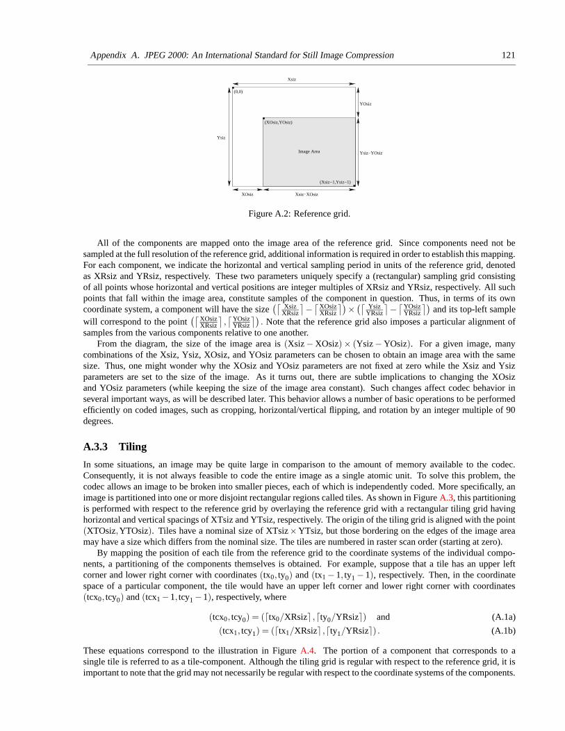
Appendix A. JPEG 2000: An International Standard for Still Image Compression 121
(Xsiz−1,Ysiz−1)
(XOsiz,YOsiz)
Xsiz−XOsiz
Image Area
(0,0)
Xsiz
Ysiz−YOsiz
Ysiz
XOsiz
YOsiz
Figure A.2: Reference grid.
All of the components are mapped onto the image area of the reference grid. Since components need not besampled at the full resolution of the reference grid, additional information is required in order to establish this mapping.For each component, we indicate the horizontal and vertical sampling period in units of the reference grid, denotedas XRsiz and YRsiz, respectively. These two parameters uniquely specify a (rectangular) sampling grid consistingof all points whose horizontal and vertical positions are integer multiples of XRsiz and YRsiz, respectively. All suchpoints that fall within the image area, constitute samples of the component in question. Thus, in terms of its owncoordinate system, a component will have the size
(⌈Xsiz
XRsiz
⌉−⌈
XOsizXRsiz
⌉)×(⌈
YsizYRsiz
⌉−⌈
YOsizYRsiz
⌉)and its top-left sample
will correspond to the point(⌈
XOsizXRsiz
⌉,⌈
YOsizYRsiz
⌉). Note that the reference grid also imposes a particular alignment of
samples from the various components relative to one another.From the diagram, the size of the image area is (Xsiz−XOsiz)× (Ysiz−YOsiz). For a given image, many
combinations of the Xsiz, Ysiz, XOsiz, and YOsiz parameters can be chosen to obtain an image area with the samesize. Thus, one might wonder why the XOsiz and YOsiz parameters are not fixed at zero while the Xsiz and Ysizparameters are set to the size of the image. As it turns out, there are subtle implications to changing the XOsizand YOsiz parameters (while keeping the size of the image area constant). Such changes affect codec behavior inseveral important ways, as will be described later. This behavior allows a number of basic operations to be performedefficiently on coded images, such as cropping, horizontal/vertical flipping, and rotation by an integer multiple of 90degrees.
A.3.3 Tiling
In some situations, an image may be quite large in comparison to the amount of memory available to the codec.Consequently, it is not always feasible to code the entire image as a single atomic unit. To solve this problem, thecodec allows an image to be broken into smaller pieces, each of which is independently coded. More specifically, animage is partitioned into one or more disjoint rectangular regions called tiles. As shown in Figure A.3, this partitioningis performed with respect to the reference grid by overlaying the reference grid with a rectangular tiling grid havinghorizontal and vertical spacings of XTsiz and YTsiz, respectively. The origin of the tiling grid is aligned with the point(XTOsiz,YTOsiz). Tiles have a nominal size of XTsiz×YTsiz, but those bordering on the edges of the image areamay have a size which differs from the nominal size. The tiles are numbered in raster scan order (starting at zero).
By mapping the position of each tile from the reference grid to the coordinate systems of the individual compo-nents, a partitioning of the components themselves is obtained. For example, suppose that a tile has an upper leftcorner and lower right corner with coordinates (tx0, ty0) and (tx1 − 1, ty1 − 1), respectively. Then, in the coordinatespace of a particular component, the tile would have an upper left corner and lower right corner with coordinates(tcx0, tcy0) and (tcx1 −1, tcy1 −1), respectively, where
(tcx0, tcy0) = (dtx0/XRsize ,dty0/YRsize) and (A.1a)
(tcx1, tcy1) = (dtx1/XRsize ,dty1/YRsize) . (A.1b)
These equations correspond to the illustration in Figure A.4. The portion of a component that corresponds to asingle tile is referred to as a tile-component. Although the tiling grid is regular with respect to the reference grid, it isimportant to note that the grid may not necessarily be regular with respect to the coordinate systems of the components.
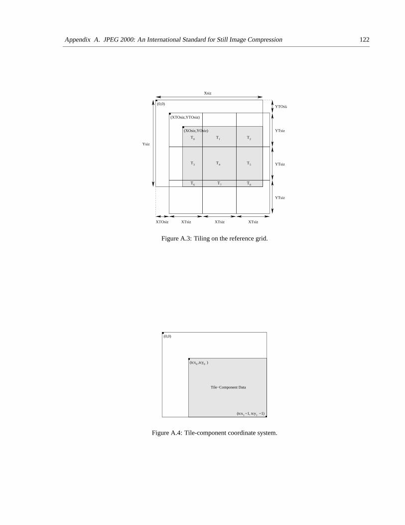
Appendix A. JPEG 2000: An International Standard for Still Image Compression 122
T7
T0 T1 T2
T3 T4 T5
T6 T8
(XOsiz,YOsiz)
(0,0)
(XTOsiz,YTOsiz)
XTOsiz XTsiz XTsiz XTsiz
YTsiz
YTsiz
YTsiz
YTOsiz
Ysiz
Xsiz
Figure A.3: Tiling on the reference grid.
tcx0 tcy0
tcx1 tcy1
(0,0)
Tile−Component Data
( , )
( −1, −1)
Figure A.4: Tile-component coordinate system.
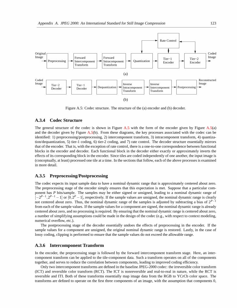
Appendix A. JPEG 2000: An International Standard for Still Image Compression 123
PreprocessingForwardIntercomponentTransform
ForwardIntracomponentTransform
QuantizationTier−1Encoder
Tier−2Encoder
CodedImage
Rate Control
OriginalImage
(a)
Tier−2Decoder
Tier−1Decoder
InverseIntracomponentTransform
PostprocessingDequantizationInverseIntercomponentTransform
CodedImage
ReconstructedImage
(b)
Figure A.5: Codec structure. The structure of the (a) encoder and (b) decoder.
A.3.4 Codec Structure
The general structure of the codec is shown in Figure A.5 with the form of the encoder given by Figure A.5(a)and the decoder given by Figure A.5(b). From these diagrams, the key processes associated with the codec can beidentified: 1) preprocessing/postprocessing, 2) intercomponent transform, 3) intracomponent transform, 4) quantiza-tion/dequantization, 5) tier-1 coding, 6) tier-2 coding, and 7) rate control. The decoder structure essentially mirrorsthat of the encoder. That is, with the exception of rate control, there is a one-to-one correspondence between functionalblocks in the encoder and decoder. Each functional block in the decoder either exactly or approximately inverts theeffects of its corresponding block in the encoder. Since tiles are coded independently of one another, the input image is(conceptually, at least) processed one tile at a time. In the sections that follow, each of the above processes is examinedin more detail.
A.3.5 Preprocessing/Postprocessing
The codec expects its input sample data to have a nominal dynamic range that is approximately centered about zero.The preprocessing stage of the encoder simply ensures that this expectation is met. Suppose that a particular com-ponent has P bits/sample. The samples may be either signed or unsigned, leading to a nominal dynamic range of[−2P−1,2P−1 −1] or [0,2P −1], respectively. If the sample values are unsigned, the nominal dynamic range is clearlynot centered about zero. Thus, the nominal dynamic range of the samples is adjusted by subtracting a bias of 2P−1
from each of the sample values. If the sample values for a component are signed, the nominal dynamic range is alreadycentered about zero, and no processing is required. By ensuring that the nominal dynamic range is centered about zero,a number of simplifying assumptions could be made in the design of the codec (e.g., with respect to context modeling,numerical overflow, etc.).
The postprocessing stage of the decoder essentially undoes the effects of preprocessing in the encoder. If thesample values for a component are unsigned, the original nominal dynamic range is restored. Lastly, in the case oflossy coding, clipping is performed to ensure that the sample values do not exceed the allowable range.
A.3.6 Intercomponent Transform
In the encoder, the preprocessing stage is followed by the forward intercomponent transform stage. Here, an inter-component transform can be applied to the tile-component data. Such a transform operates on all of the componentstogether, and serves to reduce the correlation between components, leading to improved coding efficiency.
Only two intercomponent transforms are defined in the baseline JPEG-2000 codec: the irreversible color transform(ICT) and reversible color transform (RCT). The ICT is nonreversible and real-to-real in nature, while the RCT isreversible and ITI. Both of these transforms essentially map image data from the RGB to YCrCb color space. Thetransforms are defined to operate on the first three components of an image, with the assumption that components 0,
Appendix A. JPEG 2000: An International Standard for Still Image Compression 124
1, and 2 correspond to the red, green, and blue color planes. Due to the nature of these transforms, the components onwhich they operate must be sampled at the same resolution (i.e., have the same size). As a consequence of the abovefacts, the ICT and RCT can only be employed when the image being coded has at least three components, and the firstthree components are sampled at the same resolution. The ICT may only be used in the case of lossy coding, while theRCT can be used in either the lossy or lossless case. Even if a transform can be legally employed, it is not necessaryto do so. That is, the decision to use a multicomponent transform is left at the discretion of the encoder. After theintercomponent transform stage in the encoder, data from each component is treated independently.
The ICT is nothing more than the classic RGB to YCrCb color space transform. The forward transform is definedas
V0(x,y)V1(x,y)V2(x,y)
=
0.299 0.587 0.114−0.16875 −0.33126 0.5
0.5 −0.41869 −0.08131
U0(x,y)U1(x,y)U2(x,y)
(A.2)
where U0(x,y), U1(x,y), and U2(x,y) are the input components corresponding to the red, green, and blue color planes,respectively, and V0(x,y), V1(x,y), and V2(x,y) are the output components corresponding to the Y, Cr, and Cb planes,respectively. The inverse transform can be shown to be
U0(x,y)U1(x,y)U2(x,y)
=
1 0 1.4021 −0.34413 −0.714141 −1.772 0
V0(x,y)V1(x,y)V2(x,y)
. (A.3)
The RCT is simply a reversible ITI approximation to the ICT (similar to that proposed in [59]). The forwardtransform is given by
V0(x,y) =⌊
14 (U0(x,y)+2U1(x,y)+U2(x,y))
⌋, (A.4a)
V1(x,y) = U2(x,y)−U1(x,y), and (A.4b)
V2(x,y) = U0(x,y)−U1(x,y), (A.4c)
where U0(x,y), U1(x,y), U2(x,y), V0(x,y), V1(x,y), and V2(x,y) are defined as above. The inverse transform can beshown to be
U1(x,y) = V0(x,y)−⌊
14 (V1(x,y)+V2(x,y))
⌋, (A.5a)
U0(x,y) = V2(x,y)+U1(x,y), and (A.5b)
U2(x,y) = V1(x,y)+U1(x,y). (A.5c)
The inverse intercomponent transform stage in the decoder essentially undoes the effects of the forward intercom-ponent transform stage in the encoder. If a multicomponent transform was applied during encoding, its inverse isapplied here. Unless the transform is reversible, however, the inversion may only be approximate due to the effects offinite-precision arithmetic.
A.3.7 Intracomponent Transform
Following the intercomponent transform stage in the encoder is the intracomponent transform stage. In this stage,transforms that operate on individual components can be applied. The particular type of operator employed for thispurpose is the wavelet transform. Through the application of the wavelet transform, a component is split into numerousfrequency bands (i.e., subbands). Due to the statistical properties of these subband signals, the transformed data canusually be coded more efficiently than the original untransformed data.
Both reversible ITI [40, 44, 1, 16] and nonreversible real-to-real wavelet transforms are employed by the baselinecodec. The basic building block for such transforms is the one-dimensional (1D) two-channel perfect-reconstruction(PR) uniformly maximally-decimated (UMD) filter bank which has the general form shown in Figure A.6. Here,we focus on the lifting realization of the UMD filter bank [130, 131], as it can be used to implement the reversibleITI and nonreversible real-to-real wavelet transforms employed by the baseline codec. In fact, for this reason, it islikely that this realization strategy will be employed by many codec implementations. The analysis side of the UMDfilter bank, depicted in Figure A.6(a), is associated with the forward transform, while the synthesis side, depictedin Figure A.6(b), is associated with the inverse transform. In the diagram, the {Ai(z)}λ−1
i=0 , {Qi(x)}λ−1i=0 , and {si}1
i=0
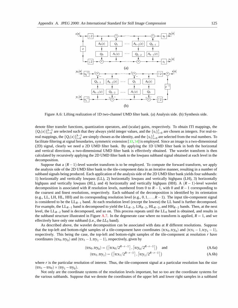
Appendix A. JPEG 2000: An International Standard for Still Image Compression 125
h+ h+
h+ h+
↓2
↓2
z
-- -- - -
-- - - -?
?
-
?
6
6
6
6
6
6
?
?
?
- -
-?
?
-
-
· · ·· · ·
s0
· · · s1
· · ·
A0(z)
x[n]
A1(z)
Aλ−2(z)
Aλ−1(z)Qλ−2
Qλ−1
Q0
Q1
y0[n]
y1[n]
(a)h+ h+
h+ h+
↑2
↑2
z−1
h+-?
- - -
6?
- -
-- ?- - -6?-
6
6
6
6? ?
-
-
-
6
6
-
-
· · ·· · ·
· · ·· · ·
+
+
+
+ −
−
−
−A0(z)
Aλ−1(z)
Aλ−2(z)
A1(z)
x[n]
Qλ−1
Qλ−2
Q1
Q0
s−11
s−10
y0[n]
y1[n]
(b)
Figure A.6: Lifting realization of 1D two-channel UMD filter bank. (a) Analysis side. (b) Synthesis side.
denote filter transfer functions, quantization operators, and (scalar) gains, respectively. To obtain ITI mappings, the{Qi(x)}λ−1
i=0 are selected such that they always yield integer values, and the {si}1i=0 are chosen as integers. For real-to-
real mappings, the {Qi(x)}λ−1i=0 are simply chosen as the identity, and the {si}1
i=0 are selected from the real numbers. Tofacilitate filtering at signal boundaries, symmetric extension [33,34] is employed. Since an image is a two-dimensional(2D) signal, clearly we need a 2D UMD filter bank. By applying the 1D UMD filter bank in both the horizontaland vertical directions, a two-dimensional UMD filter bank is effectively obtained. The wavelet transform is thencalculated by recursively applying the 2D UMD filter bank to the lowpass subband signal obtained at each level in thedecomposition.
Suppose that a (R− 1)-level wavelet transform is to be employed. To compute the forward transform, we applythe analysis side of the 2D UMD filter bank to the tile-component data in an iterative manner, resulting in a number ofsubband signals being produced. Each application of the analysis side of the 2D UMD filter bank yields four subbands:1) horizontally and vertically lowpass (LL), 2) horizontally lowpass and vertically highpass (LH), 3) horizontallyhighpass and vertically lowpass (HL), and 4) horizontally and vertically highpass (HH). A (R − 1)-level waveletdecomposition is associated with R resolution levels, numbered from 0 to R− 1, with 0 and R− 1 corresponding tothe coarsest and finest resolutions, respectively. Each subband of the decomposition is identified by its orientation(e.g., LL, LH, HL, HH) and its corresponding resolution level (e.g., 0,1, . . . ,R− 1). The input tile-component signalis considered to be the LLR−1 band. At each resolution level (except the lowest) the LL band is further decomposed.For example, the LLR−1 band is decomposed to yield the LLR−2, LHR−2, HLR−2, and HHR−2 bands. Then, at the nextlevel, the LLR−2 band is decomposed, and so on. This process repeats until the LL0 band is obtained, and results inthe subband structure illustrated in Figure A.7. In the degenerate case where no transform is applied, R = 1, and weeffectively have only one subband (i.e., the LL0 band).
As described above, the wavelet decomposition can be associated with data at R different resolutions. Supposethat the top-left and bottom-right samples of a tile-component have coordinates (tcx0, tcy0) and (tcx1 − 1, tcy1 − 1),respectively. This being the case, the top-left and bottom-right samples of the tile-component at resolution r havecoordinates (trx0, try0) and (trx1 −1, try1 −1), respectively, given by
(trx0, try0) =(⌈
tcx0/2R−r−1⌉ ,⌈tcy0/2R−r−1⌉) and (A.6a)
(trx1, try1) =(⌈
tcx1/2R−r−1⌉ ,⌈tcy1/2R−r−1⌉) (A.6b)
where r is the particular resolution of interest. Thus, the tile-component signal at a particular resolution has the size(trx1 − trx0)× (try1 − try0).
Not only are the coordinate systems of the resolution levels important, but so too are the coordinate systems forthe various subbands. Suppose that we denote the coordinates of the upper left and lower right samples in a subband
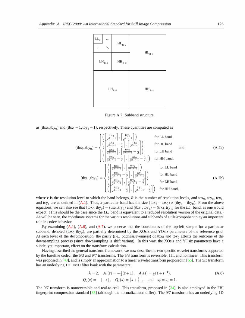
Appendix A. JPEG 2000: An International Standard for Still Image Compression 126
LL 0
R−2HHLHR−2
HLR−2
HLR−1
HHR−1LHR−1
...
... ...
Figure A.7: Subband structure.
as (tbx0, tby0) and (tbx1 −1, tby1 −1), respectively. These quantities are computed as
(tbx0, tby0) =
(⌈tcx0
2R−r−1
⌉
,⌈
tcy02R−r−1
⌉)
for LL band(⌈
tcx02R−r−1 − 1
2
⌉
,⌈
tcy02R−r−1
⌉)
for HL band(⌈
tcx02R−r−1
⌉
,⌈
tcy02R−r−1 − 1
2
⌉)
for LH band(⌈
tcx02R−r−1 − 1
2
⌉
,⌈
tcy02R−r−1 − 1
2
⌉)
for HH band,
and (A.7a)
(tbx1, tby1) =
(⌈tcx1
2R−r−1
⌉
,⌈
tcy12R−r−1
⌉)
for LL band(⌈
tcx12R−r−1 − 1
2
⌉
,⌈
tcy12R−r−1
⌉)
for HL band(⌈
tcx12R−r−1
⌉
,⌈
tcy12R−r−1 − 1
2
⌉)
for LH band(⌈
tcx12R−r−1 − 1
2
⌉
,⌈
tcy12R−r−1 − 1
2
⌉)
for HH band,
(A.7b)
where r is the resolution level to which the band belongs, R is the number of resolution levels, and tcx0, tcy0, tcx1,and tcy1 are as defined in (A.1). Thus, a particular band has the size (tbx1 − tbx0)× (tby1 − tby0). From the aboveequations, we can also see that (tbx0, tby0) = (trx0, try0) and (tbx1, tby1) = (trx1, try1) for the LLr band, as one wouldexpect. (This should be the case since the LLr band is equivalent to a reduced resolution version of the original data.)As will be seen, the coordinate systems for the various resolutions and subbands of a tile-component play an importantrole in codec behavior.
By examining (A.1), (A.6), and (A.7), we observe that the coordinates of the top-left sample for a particularsubband, denoted (tbx0, tby0), are partially determined by the XOsiz and YOsiz parameters of the reference grid.At each level of the decomposition, the parity (i.e., oddness/evenness) of tbx0 and tby0 affects the outcome of thedownsampling process (since downsampling is shift variant). In this way, the XOsiz and YOsiz parameters have asubtle, yet important, effect on the transform calculation.
Having described the general transform framework, we now describe the two specific wavelet transforms supportedby the baseline codec: the 5/3 and 9/7 transforms. The 5/3 transform is reversible, ITI, and nonlinear. This transformwas proposed in [40], and is simply an approximation to a linear wavelet transform proposed in [55]. The 5/3 transformhas an underlying 1D UMD filter bank with the parameters:
λ = 2, A0(z) = − 12 (z+1), A1(z) = 1
4 (1+ z−1), (A.8)
Q0(x) = −b−xc , Q1(x) =⌊x+ 1
2
⌋, and s0 = s1 = 1.
The 9/7 transform is nonreversible and real-to-real. This transform, proposed in [24], is also employed in the FBIfingerprint compression standard [35] (although the normalizations differ). The 9/7 transform has an underlying 1D

Appendix A. JPEG 2000: An International Standard for Still Image Compression 127
UMD filter bank with the parameters:
λ = 4, A0(z) = α0(z+1), A1(z) = α1(1+ z−1), (A.9)
A2(z) = α2(z+1), A3(z) = α3(1+ z−1),
Qi(x) = x for i = 0,1,2,3,
α0 ≈−1.586134, α1 ≈−0.052980, α2 ≈ 0.882911,
α3 ≈ 0.443506, s0 ≈ 1.230174, and s1 = 1/s0.
Since the 5/3 transform is reversible, it can be employed for either lossy or lossless coding. The 9/7 transform,lacking the reversible property, can only be used for lossy coding. The number of resolution levels is a parameter ofeach transform. A typical value for this parameter is six (for a sufficiently large image). The encoder may transformall, none, or a subset of the components. This choice is at the encoder’s discretion.
The inverse intracomponent transform stage in the decoder essentially undoes the effects of the forward intracom-ponent transform stage in the encoder. If a transform was applied to a particular component during encoding, thecorresponding inverse transform is applied here. Due to the effects of finite-precision arithmetic, the inversion processis not guaranteed to be exact unless reversible transforms are employed.
A.3.8 Quantization/Dequantization
In the encoder, after the tile-component data has been transformed (by intercomponent and/or intracomponent trans-forms), the resulting coefficients are quantized. Quantization allows greater compression to be achieved, by repre-senting transform coefficients with only the minimal precision required to obtain the desired level of image quality.Quantization of transform coefficients is one of the two primary sources of information loss in the coding path (theother source being the discarding of coding pass data as will be described later).
Transform coefficients are quantized using scalar quantization with a deadzone. A different quantizer is employedfor the coefficients of each subband, and each quantizer has only one parameter, its step size. Mathematically, thequantization process is defined as
V (x,y) = b|U(x,y)|/∆csgnU(x,y) (A.10)
where ∆ is the quantizer step size, U(x,y) is the input subband signal, and V (x,y) denotes the output quantizer indicesfor the subband. Since this equation is specified in an informative clause of the standard, encoders need not use thisprecise formula. This said, however, it is likely that many encoders will, in fact, use the above equation.
The baseline codec has two distinct modes of operation, referred to herein as integer mode and real mode. Ininteger mode, all transforms employed are ITI in nature (e.g., RCT, 5/3). In real mode, real-to-real transforms areemployed (e.g., ICT, 9/7). In integer mode, the quantizer step sizes are always fixed at one, effectively bypassingquantization and forcing the quantizer indices and transform coefficients to be one and the same. In this case, lossycoding is still possible, but rate control is achieved by another mechanism (to be discussed later). In the case of realmode (which implies lossy coding), the quantizer step sizes are chosen in conjunction with rate control. Numerousstrategies are possible for the selection of the quantizer step sizes, as will be discussed later in Section A.3.12.
As one might expect, the quantizer step sizes used by the encoder are conveyed to the decoder via the code stream.In passing, we note that the step sizes specified in the code stream are relative and not absolute quantities. That is, thequantizer step size for each band is specified relative to the nominal dynamic range of the subband signal.
In the decoder, the dequantization stage tries to undo the effects of quantization. Unless all of the quantizer stepsizes are less than or equal to one, the quantization process will normally result in some information loss, and thisinversion process is only approximate. The quantized transform coefficient values are obtained from the quantizerindices. Mathematically, the dequantization process is defined as
U(x,y) = (V (x,y)+ r sgnV (x,y))∆ (A.11)
where ∆ is the quantizer step size, r is a bias parameter, V (x,y) are the input quantizer indices for the subband, andU(x,y) is the reconstructed subband signal. Although the value of r is not normatively specified in the standard, it islikely that many decoders will use the value of one half.
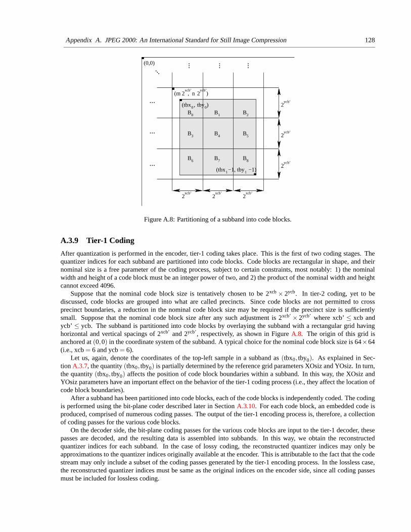
Appendix A. JPEG 2000: An International Standard for Still Image Compression 128
tbx0 tby0( , )
tbx1 tby1( −1, −1)
B0 B2
B5B4B3
B1
B6 B7 B8
2xcb’
2xcb’
2xcb’
2ycb’
2ycb’
2ycb’
2xcb’
2ycb’
(m , n )
(0,0)...
... ... ...
...
...
...
Figure A.8: Partitioning of a subband into code blocks.
A.3.9 Tier-1 Coding
After quantization is performed in the encoder, tier-1 coding takes place. This is the first of two coding stages. Thequantizer indices for each subband are partitioned into code blocks. Code blocks are rectangular in shape, and theirnominal size is a free parameter of the coding process, subject to certain constraints, most notably: 1) the nominalwidth and height of a code block must be an integer power of two, and 2) the product of the nominal width and heightcannot exceed 4096.
Suppose that the nominal code block size is tentatively chosen to be 2xcb × 2ycb. In tier-2 coding, yet to bediscussed, code blocks are grouped into what are called precincts. Since code blocks are not permitted to crossprecinct boundaries, a reduction in the nominal code block size may be required if the precinct size is sufficientlysmall. Suppose that the nominal code block size after any such adjustment is 2xcb’ × 2ycb’ where xcb’ ≤ xcb andycb’ ≤ ycb. The subband is partitioned into code blocks by overlaying the subband with a rectangular grid havinghorizontal and vertical spacings of 2xcb’ and 2ycb’, respectively, as shown in Figure A.8. The origin of this grid isanchored at (0,0) in the coordinate system of the subband. A typical choice for the nominal code block size is 64×64(i.e., xcb = 6 and ycb = 6).
Let us, again, denote the coordinates of the top-left sample in a subband as (tbx0, tby0). As explained in Sec-tion A.3.7, the quantity (tbx0, tby0) is partially determined by the reference grid parameters XOsiz and YOsiz. In turn,the quantity (tbx0, tby0) affects the position of code block boundaries within a subband. In this way, the XOsiz andYOsiz parameters have an important effect on the behavior of the tier-1 coding process (i.e., they affect the location ofcode block boundaries).
After a subband has been partitioned into code blocks, each of the code blocks is independently coded. The codingis performed using the bit-plane coder described later in Section A.3.10. For each code block, an embedded code isproduced, comprised of numerous coding passes. The output of the tier-1 encoding process is, therefore, a collectionof coding passes for the various code blocks.
On the decoder side, the bit-plane coding passes for the various code blocks are input to the tier-1 decoder, thesepasses are decoded, and the resulting data is assembled into subbands. In this way, we obtain the reconstructedquantizer indices for each subband. In the case of lossy coding, the reconstructed quantizer indices may only beapproximations to the quantizer indices originally available at the encoder. This is attributable to the fact that the codestream may only include a subset of the coding passes generated by the tier-1 encoding process. In the lossless case,the reconstructed quantizer indices must be same as the original indices on the encoder side, since all coding passesmust be included for lossless coding.

Appendix A. JPEG 2000: An International Standard for Still Image Compression 129
h0
v0
h1
v1
x
(a)
h0
v0d0
h1
d3
d1
d2 v1
x
(b)
Figure A.9: Templates for context selection. The (a) 4-connected and (b) 8-connected neighbors.
A.3.10 Bit-Plane Coding
The tier-1 coding process is essentially one of bit-plane coding. After all of the subbands have been partitionedinto code blocks, each of the resulting code blocks is independently coded using a bit-plane coder. Although thebit-plane coding technique employed is similar to those used in the embedded zerotree wavelet (EZW) [119] and setpartitioning in hierarchical trees (SPIHT) [115] codecs, there are two notable differences: 1) no interband dependenciesare exploited, and 2) there are three coding passes per bit plane instead of two. The first difference follows from thefact that each code block is completely contained within a single subband, and code blocks are coded independentlyof one another. By not exploiting interband dependencies, improved error resilience can be achieved. The seconddifference is arguably less fundamental. Using three passes per bit plane instead of two reduces the amount of dataassociated with each coding pass, facilitating finer control over rate. Also, using an additional pass per bit plane allowsbetter prioritization of important data, leading to improved coding efficiency.
As noted above, there are three coding passes per bit plane. In order, these passes are as follows: 1) significance,2) refinement, and 3) cleanup. All three types of coding passes scan the samples of a code block in the same fixedorder shown in Figure A.10. The code block is partitioned into horizontal stripes, each having a nominal height offour samples. If the code block height is not a multiple of four, the height of the bottom stripe will be less than thisnominal value. As shown in the diagram, the stripes are scanned from top to bottom. Within a stripe, columns arescanned from left to right. Within a column, samples are scanned from top to bottom.
The bit-plane encoding process generates a sequence of symbols for each coding pass. Some or all of thesesymbols may be entropy coded. For the purposes of entropy coding, a context-based adaptive binary arithmetic coderis used—more specifically, the MQ coder from the JBIG2 standard (i.e., ISO/IEC 14492 [70]). For each pass, all ofthe symbols are either arithmetically coded or raw coded (i.e., the binary symbols are emitted as raw bits with simplebit stuffing). The arithmetic and raw coding processes both ensure that certain bit patterns never occur in the output,allowing such patterns to be used for error resilience purposes.
Cleanup passes always employ arithmetic coding. In the case of the significance and refinement passes, twopossibilities exist, depending on whether the so called arithmetic-coding bypass mode (also known as lazy mode) isenabled. If lazy mode is enabled, only the significance and refinement passes for the four most significant bit planes usearithmetic coding, while the remaining such passes are raw coded. Otherwise, all significance and refinement passesare arithmetically coded. The lazy mode allows the computational complexity of bit-plane coding to be significantlyreduced, by decreasing the number of symbols that must be arithmetically coded. This comes, of course, at the cost ofreduced coding efficiency.
As indicated above, coding pass data can be encoded using one of two schemes (i.e., arithmetic or raw coding).Consecutive coding passes that employ the same encoding scheme constitute what is known as a segment. All of thecoding passes in a segment can collectively form a single codeword or each coding pass can form a separate codeword.Which of these is the case is determined by the termination mode in effect. Two termination modes are supported: per-pass termination and per-segment termination. In the first case, only the last coding pass of a segment is terminated. Inthe second case, all coding passes are terminated. Terminating all coding passes facilitates improved error resilienceat the expense of decreased coding efficiency.
Since context-based arithmetic coding is employed, a means for context selection is necessary. Generally speaking,context selection is performed by examining state information for the 4-connected or 8-connected neighbors of asample as shown in Figure A.9.
In our explanation of the coding passes that follows, we focus on the encoder side as this facilitates easier under-standing. The decoder algorithms follow directly from those employed on the encoder side.
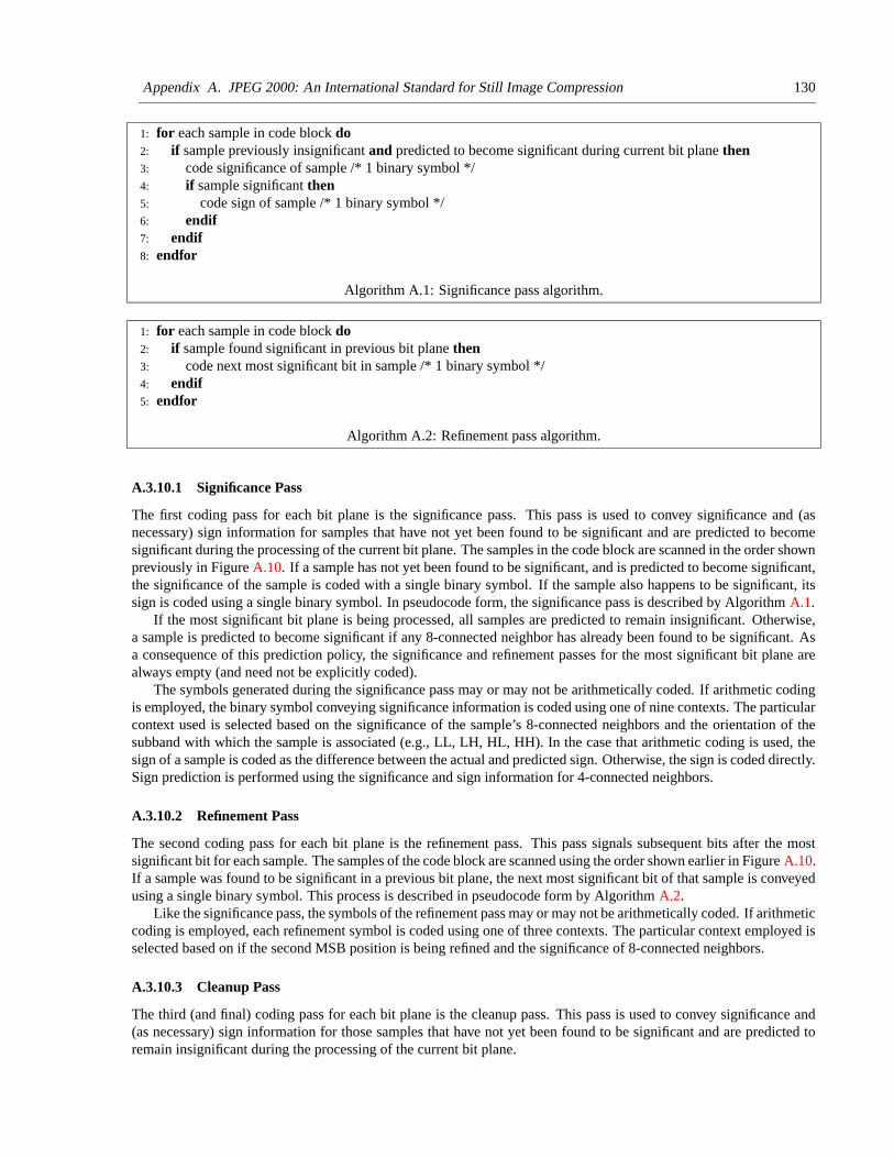
Appendix A. JPEG 2000: An International Standard for Still Image Compression 130
1: for each sample in code block do2: if sample previously insignificant and predicted to become significant during current bit plane then3: code significance of sample /* 1 binary symbol */4: if sample significant then5: code sign of sample /* 1 binary symbol */6: endif7: endif8: endfor
Algorithm A.1: Significance pass algorithm.
1: for each sample in code block do2: if sample found significant in previous bit plane then3: code next most significant bit in sample /* 1 binary symbol */4: endif5: endfor
Algorithm A.2: Refinement pass algorithm.
A.3.10.1 Significance Pass
The first coding pass for each bit plane is the significance pass. This pass is used to convey significance and (asnecessary) sign information for samples that have not yet been found to be significant and are predicted to becomesignificant during the processing of the current bit plane. The samples in the code block are scanned in the order shownpreviously in Figure A.10. If a sample has not yet been found to be significant, and is predicted to become significant,the significance of the sample is coded with a single binary symbol. If the sample also happens to be significant, itssign is coded using a single binary symbol. In pseudocode form, the significance pass is described by Algorithm A.1.
If the most significant bit plane is being processed, all samples are predicted to remain insignificant. Otherwise,a sample is predicted to become significant if any 8-connected neighbor has already been found to be significant. Asa consequence of this prediction policy, the significance and refinement passes for the most significant bit plane arealways empty (and need not be explicitly coded).
The symbols generated during the significance pass may or may not be arithmetically coded. If arithmetic codingis employed, the binary symbol conveying significance information is coded using one of nine contexts. The particularcontext used is selected based on the significance of the sample’s 8-connected neighbors and the orientation of thesubband with which the sample is associated (e.g., LL, LH, HL, HH). In the case that arithmetic coding is used, thesign of a sample is coded as the difference between the actual and predicted sign. Otherwise, the sign is coded directly.Sign prediction is performed using the significance and sign information for 4-connected neighbors.
A.3.10.2 Refinement Pass
The second coding pass for each bit plane is the refinement pass. This pass signals subsequent bits after the mostsignificant bit for each sample. The samples of the code block are scanned using the order shown earlier in Figure A.10.If a sample was found to be significant in a previous bit plane, the next most significant bit of that sample is conveyedusing a single binary symbol. This process is described in pseudocode form by Algorithm A.2.
Like the significance pass, the symbols of the refinement pass may or may not be arithmetically coded. If arithmeticcoding is employed, each refinement symbol is coded using one of three contexts. The particular context employed isselected based on if the second MSB position is being refined and the significance of 8-connected neighbors.
A.3.10.3 Cleanup Pass
The third (and final) coding pass for each bit plane is the cleanup pass. This pass is used to convey significance and(as necessary) sign information for those samples that have not yet been found to be significant and are predicted toremain insignificant during the processing of the current bit plane.
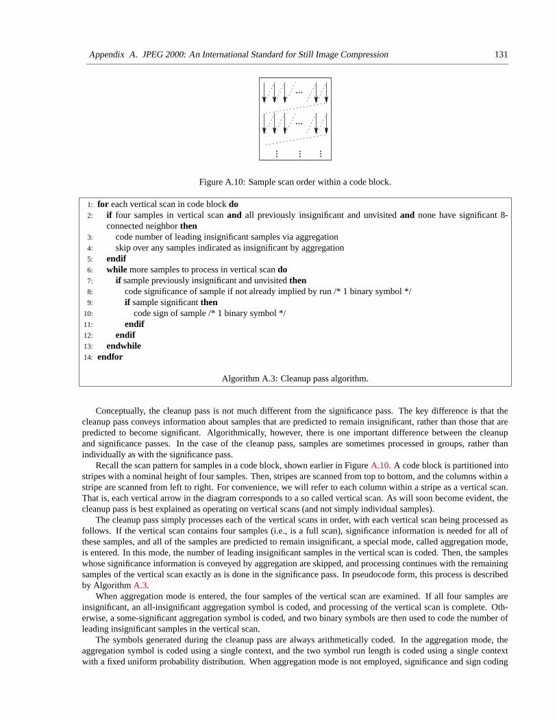
Appendix A. JPEG 2000: An International Standard for Still Image Compression 131
...
...
... ... ...
Figure A.10: Sample scan order within a code block.
1: for each vertical scan in code block do2: if four samples in vertical scan and all previously insignificant and unvisited and none have significant 8-
connected neighbor then3: code number of leading insignificant samples via aggregation4: skip over any samples indicated as insignificant by aggregation5: endif6: while more samples to process in vertical scan do7: if sample previously insignificant and unvisited then8: code significance of sample if not already implied by run /* 1 binary symbol */9: if sample significant then
10: code sign of sample /* 1 binary symbol */11: endif12: endif13: endwhile14: endfor
Algorithm A.3: Cleanup pass algorithm.
Conceptually, the cleanup pass is not much different from the significance pass. The key difference is that thecleanup pass conveys information about samples that are predicted to remain insignificant, rather than those that arepredicted to become significant. Algorithmically, however, there is one important difference between the cleanupand significance passes. In the case of the cleanup pass, samples are sometimes processed in groups, rather thanindividually as with the significance pass.
Recall the scan pattern for samples in a code block, shown earlier in Figure A.10. A code block is partitioned intostripes with a nominal height of four samples. Then, stripes are scanned from top to bottom, and the columns within astripe are scanned from left to right. For convenience, we will refer to each column within a stripe as a vertical scan.That is, each vertical arrow in the diagram corresponds to a so called vertical scan. As will soon become evident, thecleanup pass is best explained as operating on vertical scans (and not simply individual samples).
The cleanup pass simply processes each of the vertical scans in order, with each vertical scan being processed asfollows. If the vertical scan contains four samples (i.e., is a full scan), significance information is needed for all ofthese samples, and all of the samples are predicted to remain insignificant, a special mode, called aggregation mode,is entered. In this mode, the number of leading insignificant samples in the vertical scan is coded. Then, the sampleswhose significance information is conveyed by aggregation are skipped, and processing continues with the remainingsamples of the vertical scan exactly as is done in the significance pass. In pseudocode form, this process is describedby Algorithm A.3.
When aggregation mode is entered, the four samples of the vertical scan are examined. If all four samples areinsignificant, an all-insignificant aggregation symbol is coded, and processing of the vertical scan is complete. Oth-erwise, a some-significant aggregation symbol is coded, and two binary symbols are then used to code the number ofleading insignificant samples in the vertical scan.
The symbols generated during the cleanup pass are always arithmetically coded. In the aggregation mode, theaggregation symbol is coded using a single context, and the two symbol run length is coded using a single contextwith a fixed uniform probability distribution. When aggregation mode is not employed, significance and sign coding
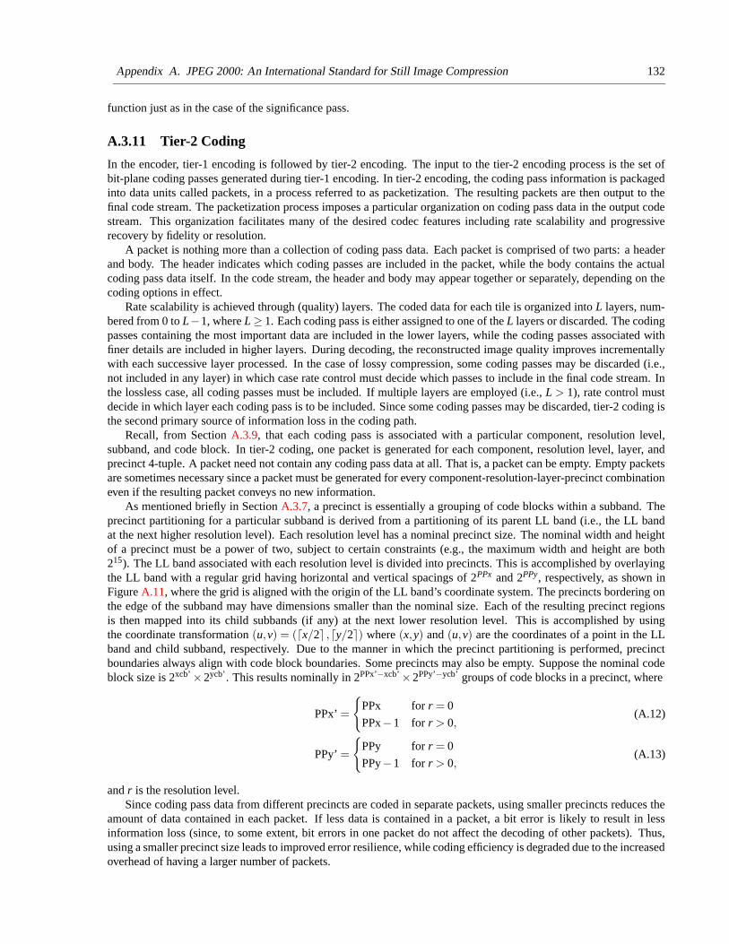
Appendix A. JPEG 2000: An International Standard for Still Image Compression 132
function just as in the case of the significance pass.
A.3.11 Tier-2 Coding
In the encoder, tier-1 encoding is followed by tier-2 encoding. The input to the tier-2 encoding process is the set ofbit-plane coding passes generated during tier-1 encoding. In tier-2 encoding, the coding pass information is packagedinto data units called packets, in a process referred to as packetization. The resulting packets are then output to thefinal code stream. The packetization process imposes a particular organization on coding pass data in the output codestream. This organization facilitates many of the desired codec features including rate scalability and progressiverecovery by fidelity or resolution.
A packet is nothing more than a collection of coding pass data. Each packet is comprised of two parts: a headerand body. The header indicates which coding passes are included in the packet, while the body contains the actualcoding pass data itself. In the code stream, the header and body may appear together or separately, depending on thecoding options in effect.
Rate scalability is achieved through (quality) layers. The coded data for each tile is organized into L layers, num-bered from 0 to L−1, where L ≥ 1. Each coding pass is either assigned to one of the L layers or discarded. The codingpasses containing the most important data are included in the lower layers, while the coding passes associated withfiner details are included in higher layers. During decoding, the reconstructed image quality improves incrementallywith each successive layer processed. In the case of lossy compression, some coding passes may be discarded (i.e.,not included in any layer) in which case rate control must decide which passes to include in the final code stream. Inthe lossless case, all coding passes must be included. If multiple layers are employed (i.e., L > 1), rate control mustdecide in which layer each coding pass is to be included. Since some coding passes may be discarded, tier-2 coding isthe second primary source of information loss in the coding path.
Recall, from Section A.3.9, that each coding pass is associated with a particular component, resolution level,subband, and code block. In tier-2 coding, one packet is generated for each component, resolution level, layer, andprecinct 4-tuple. A packet need not contain any coding pass data at all. That is, a packet can be empty. Empty packetsare sometimes necessary since a packet must be generated for every component-resolution-layer-precinct combinationeven if the resulting packet conveys no new information.
As mentioned briefly in Section A.3.7, a precinct is essentially a grouping of code blocks within a subband. Theprecinct partitioning for a particular subband is derived from a partitioning of its parent LL band (i.e., the LL bandat the next higher resolution level). Each resolution level has a nominal precinct size. The nominal width and heightof a precinct must be a power of two, subject to certain constraints (e.g., the maximum width and height are both215). The LL band associated with each resolution level is divided into precincts. This is accomplished by overlayingthe LL band with a regular grid having horizontal and vertical spacings of 2PPx and 2PPy, respectively, as shown inFigure A.11, where the grid is aligned with the origin of the LL band’s coordinate system. The precincts bordering onthe edge of the subband may have dimensions smaller than the nominal size. Each of the resulting precinct regionsis then mapped into its child subbands (if any) at the next lower resolution level. This is accomplished by usingthe coordinate transformation (u,v) = (dx/2e ,dy/2e) where (x,y) and (u,v) are the coordinates of a point in the LLband and child subband, respectively. Due to the manner in which the precinct partitioning is performed, precinctboundaries always align with code block boundaries. Some precincts may also be empty. Suppose the nominal codeblock size is 2xcb’ ×2ycb’. This results nominally in 2PPx’−xcb’ ×2PPy’−ycb’ groups of code blocks in a precinct, where
PPx’ =
{
PPx for r = 0
PPx−1 for r > 0,(A.12)
PPy’ =
{
PPy for r = 0
PPy−1 for r > 0,(A.13)
and r is the resolution level.Since coding pass data from different precincts are coded in separate packets, using smaller precincts reduces the
amount of data contained in each packet. If less data is contained in a packet, a bit error is likely to result in lessinformation loss (since, to some extent, bit errors in one packet do not affect the decoding of other packets). Thus,using a smaller precinct size leads to improved error resilience, while coding efficiency is degraded due to the increasedoverhead of having a larger number of packets.
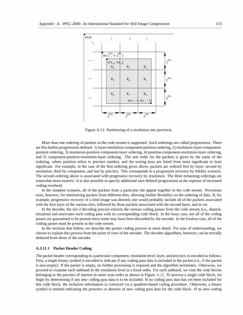
Appendix A. JPEG 2000: An International Standard for Still Image Compression 133
trx 0 try 0( , )
trx 1 try 1( −1, −1)
K0 K2
K5K4K3
K1
K6 K7 K8
2PPx
2PPx
2PPx
2PPy
2PPy
2PPy
2PPx
2PPy
(m , n )
(0,0)...
... ... ...
...
...
...
Figure A.11: Partitioning of a resolution into precincts.
More than one ordering of packets in the code stream is supported. Such orderings are called progressions. Thereare five builtin progressions defined: 1) layer-resolution-component-position ordering, 2) resolution-layer-component-position ordering, 3) resolution-position-component-layer ordering, 4) position-component-resolution-layer ordering,and 5) component-position-resolution-layer ordering. The sort order for the packets is given by the name of theordering, where position refers to precinct number, and the sorting keys are listed from most significant to leastsignificant. For example, in the case of the first ordering given above, packets are ordered first by layer, second byresolution, third by component, and last by precinct. This corresponds to a progressive recovery by fidelity scenario.The second ordering above is associated with progressive recovery by resolution. The three remaining orderings aresomewhat more esoteric. It is also possible to specify additional user-defined progressions at the expense of increasedcoding overhead.
In the simplest scenario, all of the packets from a particular tile appear together in the code stream. Provisionsexist, however, for interleaving packets from different tiles, allowing further flexibility on the ordering of data. If, forexample, progressive recovery of a tiled image was desired, one would probably include all of the packets associatedwith the first layer of the various tiles, followed by those packets associated with the second layer, and so on.
In the decoder, the tier-2 decoding process extracts the various coding passes from the code stream (i.e., depack-etization) and associates each coding pass with its corresponding code block. In the lossy case, not all of the codingpasses are guaranteed to be present since some may have been discarded by the encoder. In the lossless case, all of thecoding passes must be present in the code stream.
In the sections that follow, we describe the packet coding process in more detail. For ease of understanding, wechoose to explain this process from the point of view of the encoder. The decoder algorithms, however, can be triviallydeduced from those of the encoder.
A.3.11.1 Packet Header Coding
The packet header corresponding to a particular component, resolution level, layer, and precinct, is encoded as follows.First, a single binary symbol is encoded to indicate if any coding pass data is included in the packet (i.e., if the packetis non-empty). If the packet is empty, no further processing is required and the algorithm terminates. Otherwise, weproceed to examine each subband in the resolution level in a fixed order. For each subband, we visit the code blocksbelonging to the precinct of interest in raster scan order as shown in Figure A.12. To process a single code block, webegin by determining if any new coding pass data is to be included. If no coding pass data has yet been included forthis code block, the inclusion information is conveyed via a quadtree-based coding procedure. Otherwise, a binarysymbol is emitted indicating the presence or absence of new coding pass data for the code block. If no new coding

Appendix A. JPEG 2000: An International Standard for Still Image Compression 134
...
Figure A.12: Code block scan order with a precinct.
1: if packet not empty then2: code non-empty packet indicator /* 1 binary symbol */3: for each subband in resolution level do4: for each code block in subband precinct do5: code inclusion information /* 1 binary symbol or tag tree */6: if no new coding passes included then7: skip to next code block8: endif9: if first inclusion of code block then
10: code number of leading insignificant bit planes /* tag tree */11: endif12: code number of new coding passes13: code length increment indicator14: code length of coding pass data15: endfor16: endfor17: else18: code empty packet indicator /* 1 binary symbol */19: endif20: pad to byte boundary
Algorithm A.4: Packet header coding algorithm.
passes are included, we proceed to the processing of the next code block in the precinct. Assuming that new codingpass data are to be included, we continue with our processing of the current code block. If this is the first time codingpass data have been included for the code block, we encode the number of leading insignificant bit planes for the codeblock using a quadtree-based coding algorithm. Then, the number of new coding passes, and the length of the dataassociated with these passes is encoded. A bit stuffing algorithm is applied to all packet header data to ensure thatcertain bit patterns never occur in the output, allowing such patterns to be used for error resilience purposes. The entirepacket header coding process is summarized by Algorithm A.4.
A.3.11.2 Packet Body Coding
The algorithm used to encode the packet body is relatively simple. The code blocks are examined in the same orderas in the case of the packet header. If any new passes were specified in the corresponding packet header, the data forthese coding passes are concatenated to the packet body. This process is summarized by Algorithm A.5.
A.3.12 Rate Control
In the encoder, rate control can be achieved through two distinct mechanisms: 1) the choice of quantizer step sizes,and 2) the selection of the subset of coding passes to include in the code stream. When the integer coding mode isused (i.e., when only ITI transforms are employed) only the first mechanism may be used, since the quantizer stepsizes must be fixed at one. When the real coding mode is used, then either or both of these rate control mechanismsmay be employed.
When the first mechanism is employed, quantizer step sizes are adjusted in order to control rate. As the step sizes

Appendix A. JPEG 2000: An International Standard for Still Image Compression 135
1: for each subband in resolution level do2: for each code block in subband precinct do3: if (new coding passes included for code block) then4: output coding pass data5: endif6: endfor7: endfor
Algorithm A.5: Packet body coding algorithm.
are increased, the rate decreases, at the cost of greater distortion. Although this rate control mechanism is concep-tually simple, it does have one potential drawback. Every time the quantizer step sizes are changed, the quantizerindices change, and tier-1 encoding must be performed again. Since tier-1 coding requires a considerable amount ofcomputation, this approach to rate control may not be practical in computationally-constrained encoders.
When the second mechanism is used, the encoder can elect to discard coding passes in order to control the rate.The encoder knows the contribution that each coding pass makes to rate, and can also calculate the distortion reductionassociated with each coding pass. Using this information, the encoder can then include the coding passes in order ofdecreasing distortion reduction per unit rate until the bit budget has been exhausted. This approach is very flexiblein that different distortion metrics can be easily accommodated (e.g., mean squared error, visually weighted meansquared error, etc.).
For a more detailed treatment of rate control, the reader is referred to [72] and [132].
A.3.13 Region of Interest Coding
The codec allows different regions of an image to be coded with differing fidelity. This feature is known as region-of-interest (ROI) coding. In order to support ROI coding, a very simple yet flexible technique is employed as describedbelow.
When an image is synthesized from its transform coefficients, each coefficient contributes only to a specific regionin the reconstruction. Thus, one way to code a ROI with greater fidelity than the rest of the image would be to identifythe coefficients contributing to the ROI, and then to encode some or all of these coefficients with greater precision thanthe others. This is, in fact, the basic premise behind the ROI coding technique employed in the JPEG-2000 codec.
When an image is to be coded with a ROI, some of the transform coefficients are identified as being more importantthan the others. The coefficients of greater importance are referred to as ROI coefficients, while the remaining coef-ficients are known as background coefficients. Noting that there is a one-to-one correspondence between transformcoefficients and quantizer indices, we further define the quantizer indices for the ROI and background coefficients asthe ROI and background quantizer indices, respectively. With this terminology introduced, we are now in a positionto describe how ROI coding fits into the rest of the coding framework.
The ROI coding functionality affects the tier-1 coding process. In the encoder, before the quantizer indices forthe various subbands are bit-plane coded, the ROI quantizer indices are scaled upwards by a power of two (i.e., bya left bit shift). This scaling is performed in such a way as to ensure that all bits of the ROI quantizer indices lie inmore significant bit planes than the potentially nonzero bits of the background quantizer indices. As a consequence,all information about ROI quantizer indices will be signalled before information about background ROI indices. Inthis way, the ROI can be reconstructed at a higher fidelity than the background.
Before the quantizer indices are bit-plane coded, the encoder examines the background quantizer indices for all ofthe subbands looking for the index with the largest magnitude. Suppose that this index has its most significant bit inbit position N − 1. All of the ROI indices are then shifted N bits to the left, and bit-plane coding proceeds as in thenon-ROI case. The ROI shift value N is included in the code stream.
During decoding, any quantizer index with nonzero bits lying in bit plane N or above can be deduced to belong tothe ROI set. After the reconstructed quantizer indices are obtained from the bit-plane decoding process, all indices inthe ROI set are then scaled down by a right shift of N bits. This undoes the effect of the scaling on the encoder side.
The ROI set can be chosen to correspond to transform coefficients affecting a particular region in an image orsubset of those affecting the region. This ROI coding technique has a number of desirable properties. First, the ROI

Appendix A. JPEG 2000: An International Standard for Still Image Compression 136
Type Length(if required)
Parameters(if required)
16 bits 16 bits variable length
Figure A.13: Marker segment structure.
Main Header
Other Marker Segments
Other Marker Segments(e.g., COD, COC, QCD, QCC, RGN, etc.)
Tile−Part Header
(e.g., COD, COC, QCD, QCC, RGN, etc.)
SOC Marker Segment
SIZ Marker Segment
SOT Marker Segment
SOD Marker Segment
Tile−Part Body
Packet Data
...
Main Trailer
EOC Marker Segment
Figure A.14: Code stream structure.
can have any arbitrary shape and be disjoint. Second, there is no need to explicitly signal the ROI set, since it can bededuced by the decoder from the ROI shift value and the magnitude of the quantizer indices.
For more information on ROI coding, the reader is referred to [46, 25].
A.3.14 Code Stream
In order to specify the coded representation of an image, two different levels of syntax are employed by the codec. Thelowest level syntax is associated with what is referred to as the code stream. The code stream is essentially a sequenceof tagged records and their accompanying data.
The basic building block of the code stream is the marker segment. As shown in Figure A.13, a marker segmentis comprised of three fields: the type, length, and parameters fields. The type (or marker) field identifies the particularkind of marker segment. The length field specifies the number of bytes in the marker segment. The parametersfield provides additional information specific to the marker type. Not all types of marker segments have length andparameters fields. The presence (or absence) of these fields is determined by the marker segment type. Each type ofmarker segment signals its own particular class of information.
A code stream is simply a sequence of marker segments and auxiliary data (i.e., packet data) organized as shownin Figure A.14. The code stream consists of a main header, followed by tile-part header and body pairs, followed bya main trailer. A list of some of the more important marker segments is given in Table A.2. Parameters specified inmarker segments in the main header serve as defaults for the entire code stream. These default settings, however, maybe overridden for a particular tile by specifying new values in a marker segment in the tile’s header.
All marker segments, packet headers, and packet bodies are a multiple of 8 bits in length. As a consequence, allmarkers are byte-aligned, and the code stream itself is always an integral number of bytes.
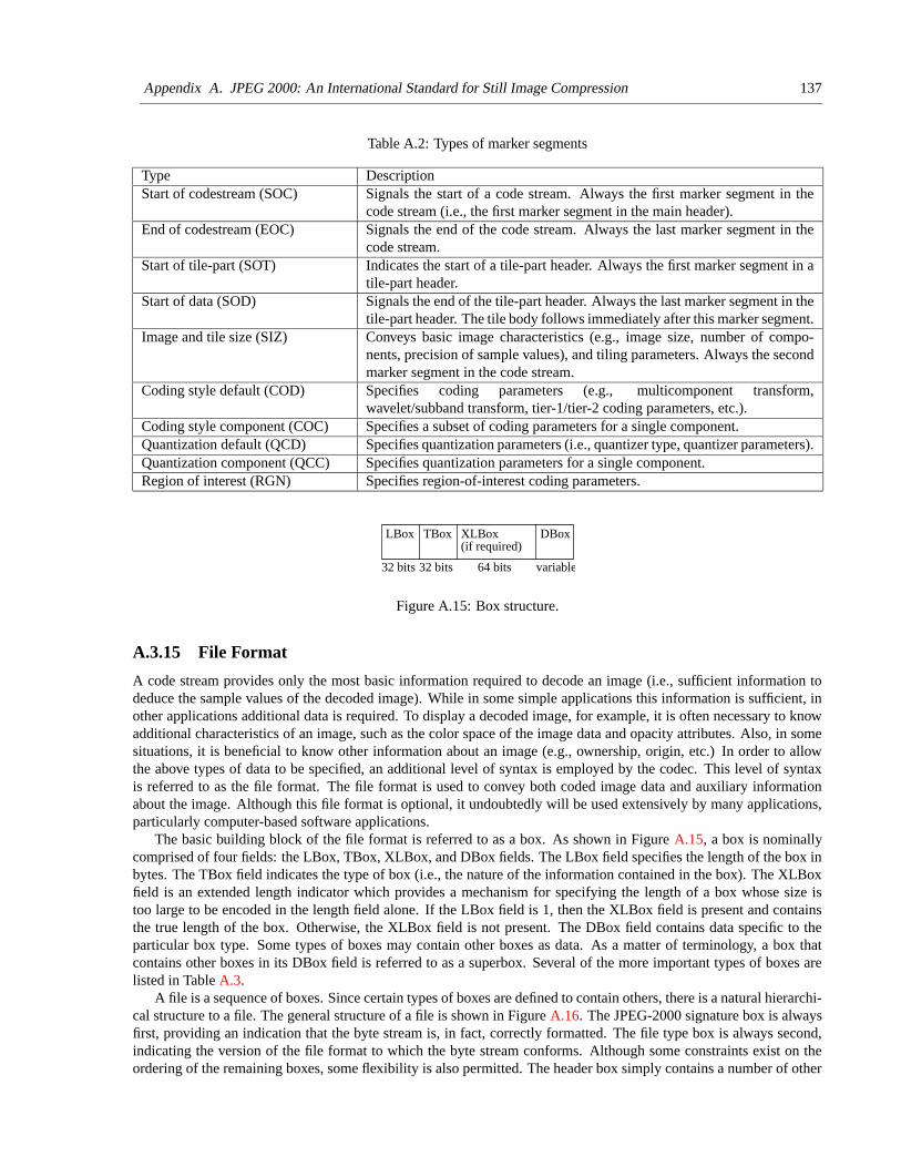
Appendix A. JPEG 2000: An International Standard for Still Image Compression 137
Table A.2: Types of marker segments
Type DescriptionStart of codestream (SOC) Signals the start of a code stream. Always the first marker segment in the
code stream (i.e., the first marker segment in the main header).End of codestream (EOC) Signals the end of the code stream. Always the last marker segment in the
code stream.Start of tile-part (SOT) Indicates the start of a tile-part header. Always the first marker segment in a
tile-part header.Start of data (SOD) Signals the end of the tile-part header. Always the last marker segment in the
tile-part header. The tile body follows immediately after this marker segment.Image and tile size (SIZ) Conveys basic image characteristics (e.g., image size, number of compo-
nents, precision of sample values), and tiling parameters. Always the secondmarker segment in the code stream.
Coding style default (COD) Specifies coding parameters (e.g., multicomponent transform,wavelet/subband transform, tier-1/tier-2 coding parameters, etc.).
Coding style component (COC) Specifies a subset of coding parameters for a single component.Quantization default (QCD) Specifies quantization parameters (i.e., quantizer type, quantizer parameters).Quantization component (QCC) Specifies quantization parameters for a single component.Region of interest (RGN) Specifies region-of-interest coding parameters.
LBox TBox XLBox(if required)
DBox
32 bits 32 bits 64 bits variable
Figure A.15: Box structure.
A.3.15 File Format
A code stream provides only the most basic information required to decode an image (i.e., sufficient information todeduce the sample values of the decoded image). While in some simple applications this information is sufficient, inother applications additional data is required. To display a decoded image, for example, it is often necessary to knowadditional characteristics of an image, such as the color space of the image data and opacity attributes. Also, in somesituations, it is beneficial to know other information about an image (e.g., ownership, origin, etc.) In order to allowthe above types of data to be specified, an additional level of syntax is employed by the codec. This level of syntaxis referred to as the file format. The file format is used to convey both coded image data and auxiliary informationabout the image. Although this file format is optional, it undoubtedly will be used extensively by many applications,particularly computer-based software applications.
The basic building block of the file format is referred to as a box. As shown in Figure A.15, a box is nominallycomprised of four fields: the LBox, TBox, XLBox, and DBox fields. The LBox field specifies the length of the box inbytes. The TBox field indicates the type of box (i.e., the nature of the information contained in the box). The XLBoxfield is an extended length indicator which provides a mechanism for specifying the length of a box whose size istoo large to be encoded in the length field alone. If the LBox field is 1, then the XLBox field is present and containsthe true length of the box. Otherwise, the XLBox field is not present. The DBox field contains data specific to theparticular box type. Some types of boxes may contain other boxes as data. As a matter of terminology, a box thatcontains other boxes in its DBox field is referred to as a superbox. Several of the more important types of boxes arelisted in Table A.3.
A file is a sequence of boxes. Since certain types of boxes are defined to contain others, there is a natural hierarchi-cal structure to a file. The general structure of a file is shown in Figure A.16. The JPEG-2000 signature box is alwaysfirst, providing an indication that the byte stream is, in fact, correctly formatted. The file type box is always second,indicating the version of the file format to which the byte stream conforms. Although some constraints exist on theordering of the remaining boxes, some flexibility is also permitted. The header box simply contains a number of other
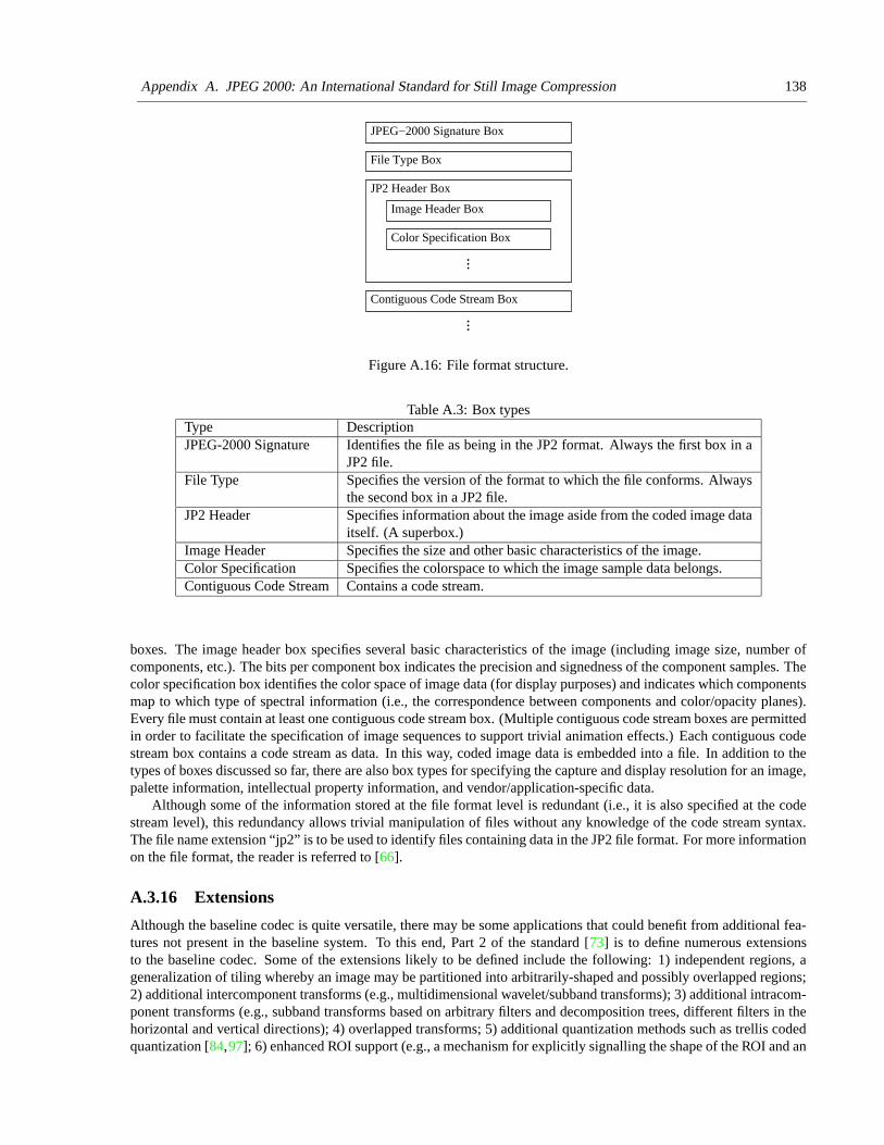
Appendix A. JPEG 2000: An International Standard for Still Image Compression 138
File Type Box
Image Header Box
Color Specification Box
JP2 Header Box
...
Contiguous Code Stream Box
JPEG−2000 Signature Box
...
Figure A.16: File format structure.
Table A.3: Box typesType DescriptionJPEG-2000 Signature Identifies the file as being in the JP2 format. Always the first box in a
JP2 file.File Type Specifies the version of the format to which the file conforms. Always
the second box in a JP2 file.JP2 Header Specifies information about the image aside from the coded image data
itself. (A superbox.)Image Header Specifies the size and other basic characteristics of the image.Color Specification Specifies the colorspace to which the image sample data belongs.Contiguous Code Stream Contains a code stream.
boxes. The image header box specifies several basic characteristics of the image (including image size, number ofcomponents, etc.). The bits per component box indicates the precision and signedness of the component samples. Thecolor specification box identifies the color space of image data (for display purposes) and indicates which componentsmap to which type of spectral information (i.e., the correspondence between components and color/opacity planes).Every file must contain at least one contiguous code stream box. (Multiple contiguous code stream boxes are permittedin order to facilitate the specification of image sequences to support trivial animation effects.) Each contiguous codestream box contains a code stream as data. In this way, coded image data is embedded into a file. In addition to thetypes of boxes discussed so far, there are also box types for specifying the capture and display resolution for an image,palette information, intellectual property information, and vendor/application-specific data.
Although some of the information stored at the file format level is redundant (i.e., it is also specified at the codestream level), this redundancy allows trivial manipulation of files without any knowledge of the code stream syntax.The file name extension “jp2” is to be used to identify files containing data in the JP2 file format. For more informationon the file format, the reader is referred to [66].
A.3.16 Extensions
Although the baseline codec is quite versatile, there may be some applications that could benefit from additional fea-tures not present in the baseline system. To this end, Part 2 of the standard [73] is to define numerous extensionsto the baseline codec. Some of the extensions likely to be defined include the following: 1) independent regions, ageneralization of tiling whereby an image may be partitioned into arbitrarily-shaped and possibly overlapped regions;2) additional intercomponent transforms (e.g., multidimensional wavelet/subband transforms); 3) additional intracom-ponent transforms (e.g., subband transforms based on arbitrary filters and decomposition trees, different filters in thehorizontal and vertical directions); 4) overlapped transforms; 5) additional quantization methods such as trellis codedquantization [84,97]; 6) enhanced ROI support (e.g., a mechanism for explicitly signalling the shape of the ROI and an
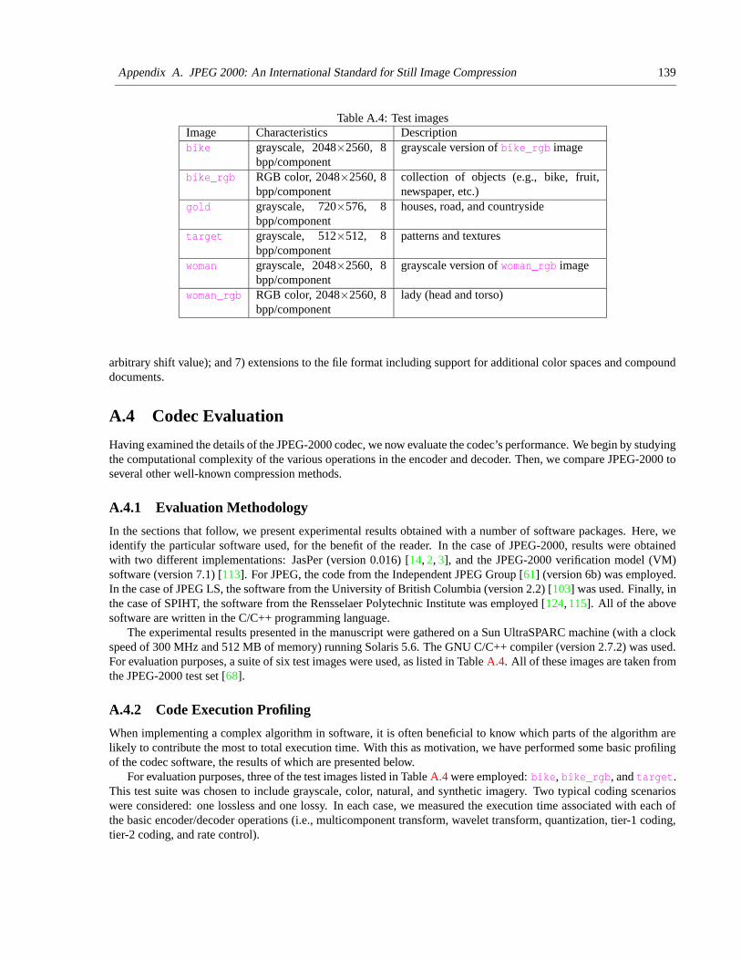
Appendix A. JPEG 2000: An International Standard for Still Image Compression 139
Table A.4: Test imagesImage Characteristics Descriptionbike grayscale, 2048×2560, 8
bpp/componentgrayscale version of bike_rgb image
bike_rgb RGB color, 2048×2560, 8bpp/component
collection of objects (e.g., bike, fruit,newspaper, etc.)
gold grayscale, 720×576, 8bpp/component
houses, road, and countryside
target grayscale, 512×512, 8bpp/component
patterns and textures
woman grayscale, 2048×2560, 8bpp/component
grayscale version of woman_rgb image
woman_rgb RGB color, 2048×2560, 8bpp/component
lady (head and torso)
arbitrary shift value); and 7) extensions to the file format including support for additional color spaces and compounddocuments.
A.4 Codec Evaluation
Having examined the details of the JPEG-2000 codec, we now evaluate the codec’s performance. We begin by studyingthe computational complexity of the various operations in the encoder and decoder. Then, we compare JPEG-2000 toseveral other well-known compression methods.
A.4.1 Evaluation Methodology
In the sections that follow, we present experimental results obtained with a number of software packages. Here, weidentify the particular software used, for the benefit of the reader. In the case of JPEG-2000, results were obtainedwith two different implementations: JasPer (version 0.016) [14, 2, 3], and the JPEG-2000 verification model (VM)software (version 7.1) [113]. For JPEG, the code from the Independent JPEG Group [61] (version 6b) was employed.In the case of JPEG LS, the software from the University of British Columbia (version 2.2) [103] was used. Finally, inthe case of SPIHT, the software from the Rensselaer Polytechnic Institute was employed [124, 115]. All of the abovesoftware are written in the C/C++ programming language.
The experimental results presented in the manuscript were gathered on a Sun UltraSPARC machine (with a clockspeed of 300 MHz and 512 MB of memory) running Solaris 5.6. The GNU C/C++ compiler (version 2.7.2) was used.For evaluation purposes, a suite of six test images were used, as listed in Table A.4. All of these images are taken fromthe JPEG-2000 test set [68].
A.4.2 Code Execution Profiling
When implementing a complex algorithm in software, it is often beneficial to know which parts of the algorithm arelikely to contribute the most to total execution time. With this as motivation, we have performed some basic profilingof the codec software, the results of which are presented below.
For evaluation purposes, three of the test images listed in Table A.4 were employed: bike, bike_rgb, and target.This test suite was chosen to include grayscale, color, natural, and synthetic imagery. Two typical coding scenarioswere considered: one lossless and one lossy. In each case, we measured the execution time associated with each ofthe basic encoder/decoder operations (i.e., multicomponent transform, wavelet transform, quantization, tier-1 coding,tier-2 coding, and rate control).
Appendix A. JPEG 2000: An International Standard for Still Image Compression 140
A.4.2.1 Lossless Coding
In the first coding scenario, the three test images were encoded in a lossless manner, and then the resulting codestreams were decoded. In each case, the encoder and decoder execution was profiled, leading to the results shown inTable A.5.
First, let us consider the case of the encoder. Examining Table A.5(a), we see that the encoder spends most of itstime on tier-1 coding and the wavelet transform. In fact, these two operations together account for the vast majority ofthe encoder’s execution time (typically 85–95%). The amount of time consumed by the multicomponent transform andtier-2 coding operations is much less significant. Examining tier-1 coding in more detail, we observe that for naturalimagery (e.g., bike, bike_rgb), significance coding usually requires the most time, followed by the cleanup coding,and then refinement coding. For synthetic imagery, however, this trend is not necessarily observed, as evidenced bythe results for the target image. Thus, the execution time breakdown for tier-1 coding is somewhat sensitive to imagecontent.
Now, let us consider the case of the decoder. The execution profiling results for the decoder are given in Ta-ble A.5(b). Again, we can see that the decoder usually spends most of its time on tier-1 coding (typically about 50%),followed next by the wavelet transform. These two operations combined account for the vast majority of the decoder’sexecution time (typically 80–95%). The multicomponent transform and tier-2 coding operations consume relativelylittle time. Examining the tier-1 coding process in more detail, we observe similar trends as in the encoder. That is, fornatural imagery, significance coding requires the most time, followed by cleanup coding, and then refinement coding,while the breakdown is less predictable for synthetic imagery.
A.4.2.2 Lossy Coding
In the second coding scenario, the three test images were encoded in a lossy manner, and then the resulting codestreams were decoded. Again, in each case, the encoder and decoder execution was profiled. This led to the resultsgiven in Table A.6.
First, let us study the results for the encoder, given in Table A.6(a). Clearly, the tier-1 coding and wavelet transformoperations require the most time. Together, these two operations account for the vast majority of the execution time(typically 75–85%). The multicomponent transform is the next biggest consumer of time (typically, requiring 10–15%). The quantization, tier-2 coding, and rate control operations require relatively little time. Looking at the tier-1coding process in more detail, we observe that the most time is usually required by cleanup coding, followed bysignificance coding, and then refinement coding.
Now, let us consider the case of the decoder. From the results in Table A.6(b), we can see that the wavelet transformclearly requires the most time by far (typically 45–70%). Tier-1 coding is the next largest time consumer, but hasmuch more modest requirements (typically 15–25%). The multicomponent transform requires almost as much time(typically 15–20%). The quantization, and tier-2 coding operations require relatively little time. Looking at the tier-1coding process in more detail, we observe that, for natural imagery, the least time is required by refinement coding.Generally speaking, the execution time breakdown for tier-1 coding depends, to a large extent, on the particular imageand bit rate employed.
In the case of both JPEG-2000 implementations considered in this study (i.e., JasPer and the VM software), ratecontrol is achieved through the selection of the coding passes to include in the final code stream. The quantizer stepsizes are fixed. To ensure optimal rate-distortion performance, the encoder generates all of the coding passes duringtier-1 coding (even though some coding passes may not be included in the final code stream). This leads to the largeamount of time consumed by tier-1 coding in the encoder. Since quantization takes place, however, the tier-1 codingoverhead is not as great (in absolute terms) as in the lossless case.
It is important to note that different multicomponent and wavelet transforms are employed in the lossy and losslesscases. In the case of lossless coding, the multicomponent and wavelet transforms employed are the RCT and 5/3,respectively. For lossy coding, the ICT and 9/7 transforms are employed, respectively. The ICT requires more compu-tation than the RCT, and similarly the 9/7 transform requires more computation than the 5/3 transform. This explainsthe larger amount of time spent on the multicomponent and wavelet transform operations relative to the lossless case.
A.4.3 JPEG 2000 vs. Other Methods
So far, we have examined the JPEG 2000 codec only in isolation. Of course, it is only natural to wonder how JPEG2000 performs in comparison to other compression methods. With this as motivation, we compare the performance

Appendix A. JPEG 2000: An International Standard for Still Image Compression 141
Table A.5: Codec execution profile for lossless coding (1 tile, SNR progressive, 1 layer, RCT for color images, 5/3wavelet transform, 5 decomposition levels). (a) Encoder. (b) Decoder.
(a)% of Execution Time
Operation bike bike_rgb targetintercomponent transform — 0.5 —intracomponent transform 40.4 42.9 46.4tier-1 coding 52.8 49.1 46.3
significance 22.0 21.5 12.9
refinement 13.1 10.5 9.5
cleanup 14.4 13.6 19.5
tier-2 coding 4.1 5.0 2.6
(b)% of Execution Time
Operation bike bike_rgb targetintercomponent transform — 0.5 —intracomponent transform 40.8 41.2 52.2tier-1 coding 51.3 45.2 39.2
significance 19.9 18.3 8.9
refinement 9.5 8.3 11.2
cleanup 11.3 8.7 6.6
tier-2 coding 3.1 8.1 1.6
Table A.6: Codec execution profile for lossy coding (32:1 compression for grayscale images and 64:1 compression forcolor images, 1 tile, SNR progressive, 1 layer, ICT for color images, 9/7 wavelet transform, 5 decomposition levels).(a) Encoder. (b) Decoder.
(a)% of Execution Time
Operation bike bike_rgb targetintercomponent transform — 12.7 —intracomponent transform 31.7 29.9 35.9quantization 3.1 2.8 3.4tier-1 coding 60.7 49.7 54.1
significance 22.5 17.8 16.6
refinement 12.5 8.6 13.5
cleanup 19.9 16.8 19.6
tier-2 coding 1.3 1.1 0.7
(b)% of Execution Time
Operation bike bike_rgb targetintercomponent transform — 18.5 —intracomponent transform 63.3 48.6 58.9quantization 6.3 4.8 5.4tier-1 coding 19.6 17.4 20.2
significance 3.7 2.4 3.6
refinement 1.1 0.6 1.5
cleanup 3.3 2.2 6.0
tier-2 coding 0.5 0.2 0.3
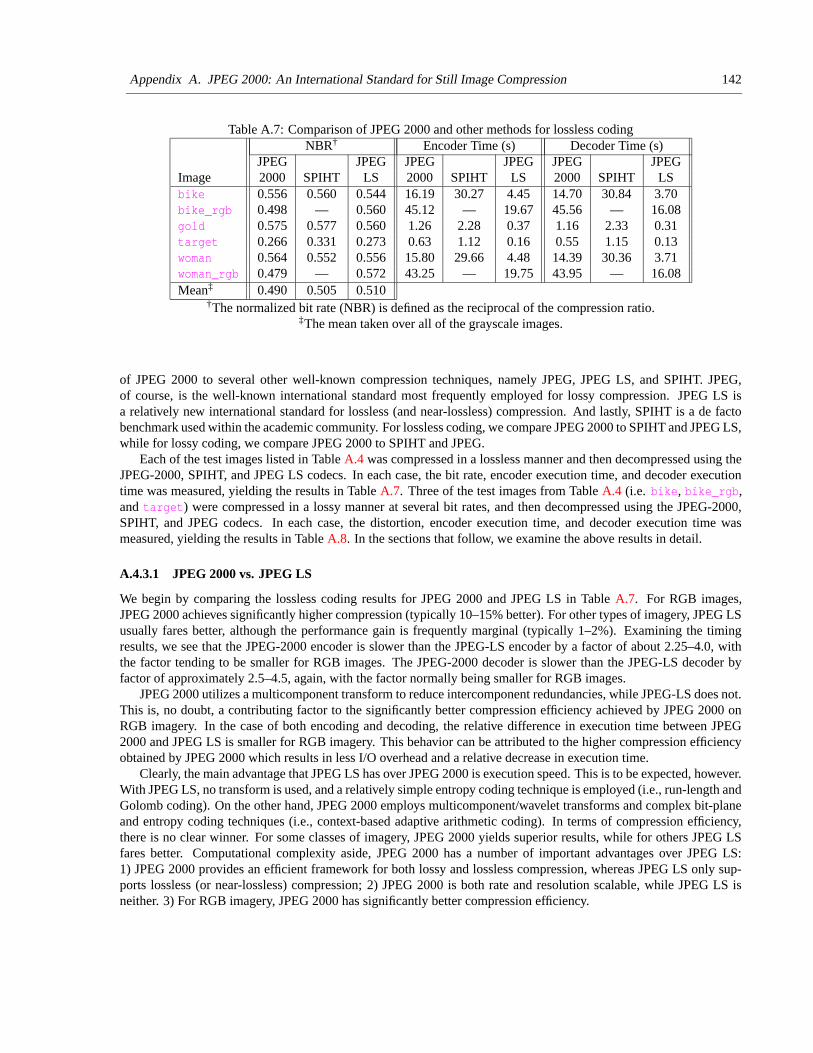
Appendix A. JPEG 2000: An International Standard for Still Image Compression 142
Table A.7: Comparison of JPEG 2000 and other methods for lossless codingNBR† Encoder Time (s) Decoder Time (s)
JPEG JPEG JPEG JPEG JPEG JPEGImage 2000 SPIHT LS 2000 SPIHT LS 2000 SPIHT LSbike 0.556 0.560 0.544 16.19 30.27 4.45 14.70 30.84 3.70bike_rgb 0.498 — 0.560 45.12 — 19.67 45.56 — 16.08gold 0.575 0.577 0.560 1.26 2.28 0.37 1.16 2.33 0.31target 0.266 0.331 0.273 0.63 1.12 0.16 0.55 1.15 0.13woman 0.564 0.552 0.556 15.80 29.66 4.48 14.39 30.36 3.71woman_rgb 0.479 — 0.572 43.25 — 19.75 43.95 — 16.08Mean‡ 0.490 0.505 0.510
†The normalized bit rate (NBR) is defined as the reciprocal of the compression ratio.‡The mean taken over all of the grayscale images.
of JPEG 2000 to several other well-known compression techniques, namely JPEG, JPEG LS, and SPIHT. JPEG,of course, is the well-known international standard most frequently employed for lossy compression. JPEG LS isa relatively new international standard for lossless (and near-lossless) compression. And lastly, SPIHT is a de factobenchmark used within the academic community. For lossless coding, we compare JPEG 2000 to SPIHT and JPEG LS,while for lossy coding, we compare JPEG 2000 to SPIHT and JPEG.
Each of the test images listed in Table A.4 was compressed in a lossless manner and then decompressed using theJPEG-2000, SPIHT, and JPEG LS codecs. In each case, the bit rate, encoder execution time, and decoder executiontime was measured, yielding the results in Table A.7. Three of the test images from Table A.4 (i.e. bike, bike_rgb,and target) were compressed in a lossy manner at several bit rates, and then decompressed using the JPEG-2000,SPIHT, and JPEG codecs. In each case, the distortion, encoder execution time, and decoder execution time wasmeasured, yielding the results in Table A.8. In the sections that follow, we examine the above results in detail.
A.4.3.1 JPEG 2000 vs. JPEG LS
We begin by comparing the lossless coding results for JPEG 2000 and JPEG LS in Table A.7. For RGB images,JPEG 2000 achieves significantly higher compression (typically 10–15% better). For other types of imagery, JPEG LSusually fares better, although the performance gain is frequently marginal (typically 1–2%). Examining the timingresults, we see that the JPEG-2000 encoder is slower than the JPEG-LS encoder by a factor of about 2.25–4.0, withthe factor tending to be smaller for RGB images. The JPEG-2000 decoder is slower than the JPEG-LS decoder byfactor of approximately 2.5–4.5, again, with the factor normally being smaller for RGB images.
JPEG 2000 utilizes a multicomponent transform to reduce intercomponent redundancies, while JPEG-LS does not.This is, no doubt, a contributing factor to the significantly better compression efficiency achieved by JPEG 2000 onRGB imagery. In the case of both encoding and decoding, the relative difference in execution time between JPEG2000 and JPEG LS is smaller for RGB imagery. This behavior can be attributed to the higher compression efficiencyobtained by JPEG 2000 which results in less I/O overhead and a relative decrease in execution time.
Clearly, the main advantage that JPEG LS has over JPEG 2000 is execution speed. This is to be expected, however.With JPEG LS, no transform is used, and a relatively simple entropy coding technique is employed (i.e., run-length andGolomb coding). On the other hand, JPEG 2000 employs multicomponent/wavelet transforms and complex bit-planeand entropy coding techniques (i.e., context-based adaptive arithmetic coding). In terms of compression efficiency,there is no clear winner. For some classes of imagery, JPEG 2000 yields superior results, while for others JPEG LSfares better. Computational complexity aside, JPEG 2000 has a number of important advantages over JPEG LS:1) JPEG 2000 provides an efficient framework for both lossy and lossless compression, whereas JPEG LS only sup-ports lossless (or near-lossless) compression; 2) JPEG 2000 is both rate and resolution scalable, while JPEG LS isneither. 3) For RGB imagery, JPEG 2000 has significantly better compression efficiency.
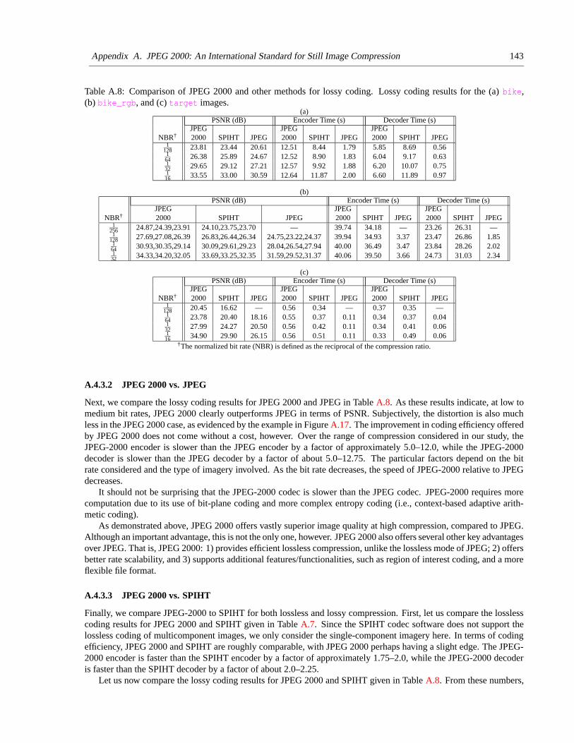
Appendix A. JPEG 2000: An International Standard for Still Image Compression 143
Table A.8: Comparison of JPEG 2000 and other methods for lossy coding. Lossy coding results for the (a) bike,(b) bike_rgb, and (c) target images.
(a)PSNR (dB) Encoder Time (s) Decoder Time (s)
JPEG JPEG JPEGNBR† 2000 SPIHT JPEG 2000 SPIHT JPEG 2000 SPIHT JPEG
1128 23.81 23.44 20.61 12.51 8.44 1.79 5.85 8.69 0.56
164 26.38 25.89 24.67 12.52 8.90 1.83 6.04 9.17 0.631
32 29.65 29.12 27.21 12.57 9.92 1.88 6.20 10.07 0.751
16 33.55 33.00 30.59 12.64 11.87 2.00 6.60 11.89 0.97
(b)PSNR (dB) Encoder Time (s) Decoder Time (s)
JPEG JPEG JPEGNBR† 2000 SPIHT JPEG 2000 SPIHT JPEG 2000 SPIHT JPEG
1256 24.87,24.39,23.91 24.10,23.75,23.70 — 39.74 34.18 — 23.26 26.31 —1
128 27.69,27.08,26.39 26.83,26.44,26.34 24.75,23.22,24.37 39.94 34.93 3.37 23.47 26.86 1.85164 30.93,30.35,29.14 30.09,29.61,29.23 28.04,26.54,27.94 40.00 36.49 3.47 23.84 28.26 2.02132 34.33,34.20,32.05 33.69,33.25,32.35 31.59,29.52,31.37 40.06 39.50 3.66 24.73 31.03 2.34
(c)PSNR (dB) Encoder Time (s) Decoder Time (s)
JPEG JPEG JPEGNBR† 2000 SPIHT JPEG 2000 SPIHT JPEG 2000 SPIHT JPEG
1128 20.45 16.62 — 0.56 0.34 — 0.37 0.35 —
164 23.78 20.40 18.16 0.55 0.37 0.11 0.34 0.37 0.041
32 27.99 24.27 20.50 0.56 0.42 0.11 0.34 0.41 0.061
16 34.90 29.90 26.15 0.56 0.51 0.11 0.33 0.49 0.06†The normalized bit rate (NBR) is defined as the reciprocal of the compression ratio.
A.4.3.2 JPEG 2000 vs. JPEG
Next, we compare the lossy coding results for JPEG 2000 and JPEG in Table A.8. As these results indicate, at low tomedium bit rates, JPEG 2000 clearly outperforms JPEG in terms of PSNR. Subjectively, the distortion is also muchless in the JPEG 2000 case, as evidenced by the example in Figure A.17. The improvement in coding efficiency offeredby JPEG 2000 does not come without a cost, however. Over the range of compression considered in our study, theJPEG-2000 encoder is slower than the JPEG encoder by a factor of approximately 5.0–12.0, while the JPEG-2000decoder is slower than the JPEG decoder by a factor of about 5.0–12.75. The particular factors depend on the bitrate considered and the type of imagery involved. As the bit rate decreases, the speed of JPEG-2000 relative to JPEGdecreases.
It should not be surprising that the JPEG-2000 codec is slower than the JPEG codec. JPEG-2000 requires morecomputation due to its use of bit-plane coding and more complex entropy coding (i.e., context-based adaptive arith-metic coding).
As demonstrated above, JPEG 2000 offers vastly superior image quality at high compression, compared to JPEG.Although an important advantage, this is not the only one, however. JPEG 2000 also offers several other key advantagesover JPEG. That is, JPEG 2000: 1) provides efficient lossless compression, unlike the lossless mode of JPEG; 2) offersbetter rate scalability, and 3) supports additional features/functionalities, such as region of interest coding, and a moreflexible file format.
A.4.3.3 JPEG 2000 vs. SPIHT
Finally, we compare JPEG-2000 to SPIHT for both lossless and lossy compression. First, let us compare the losslesscoding results for JPEG 2000 and SPIHT given in Table A.7. Since the SPIHT codec software does not support thelossless coding of multicomponent images, we only consider the single-component imagery here. In terms of codingefficiency, JPEG 2000 and SPIHT are roughly comparable, with JPEG 2000 perhaps having a slight edge. The JPEG-2000 encoder is faster than the SPIHT encoder by a factor of approximately 1.75–2.0, while the JPEG-2000 decoderis faster than the SPIHT decoder by a factor of about 2.0–2.25.
Let us now compare the lossy coding results for JPEG 2000 and SPIHT given in Table A.8. From these numbers,
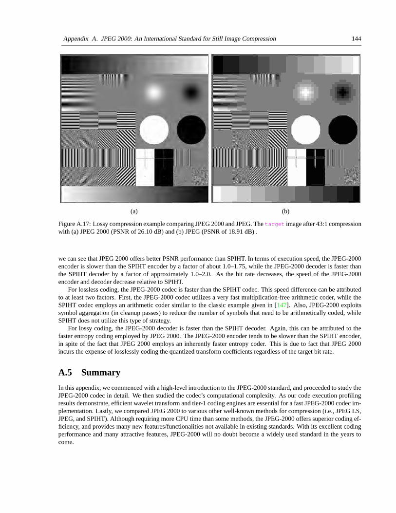
Appendix A. JPEG 2000: An International Standard for Still Image Compression 144
(a) (b)
Figure A.17: Lossy compression example comparing JPEG 2000 and JPEG. The target image after 43:1 compressionwith (a) JPEG 2000 (PSNR of 26.10 dB) and (b) JPEG (PSNR of 18.91 dB) .
we can see that JPEG 2000 offers better PSNR performance than SPIHT. In terms of execution speed, the JPEG-2000encoder is slower than the SPIHT encoder by a factor of about 1.0–1.75, while the JPEG-2000 decoder is faster thanthe SPIHT decoder by a factor of approximately 1.0–2.0. As the bit rate decreases, the speed of the JPEG-2000encoder and decoder decrease relative to SPIHT.
For lossless coding, the JPEG-2000 codec is faster than the SPIHT codec. This speed difference can be attributedto at least two factors. First, the JPEG-2000 codec utilizes a very fast multiplication-free arithmetic coder, while theSPIHT codec employs an arithmetic coder similar to the classic example given in [147]. Also, JPEG-2000 exploitssymbol aggregation (in cleanup passes) to reduce the number of symbols that need to be arithmetically coded, whileSPIHT does not utilize this type of strategy.
For lossy coding, the JPEG-2000 decoder is faster than the SPIHT decoder. Again, this can be attributed to thefaster entropy coding employed by JPEG 2000. The JPEG-2000 encoder tends to be slower than the SPIHT encoder,in spite of the fact that JPEG 2000 employs an inherently faster entropy coder. This is due to fact that JPEG 2000incurs the expense of losslessly coding the quantized transform coefficients regardless of the target bit rate.
A.5 Summary
In this appendix, we commenced with a high-level introduction to the JPEG-2000 standard, and proceeded to study theJPEG-2000 codec in detail. We then studied the codec’s computational complexity. As our code execution profilingresults demonstrate, efficient wavelet transform and tier-1 coding engines are essential for a fast JPEG-2000 codec im-plementation. Lastly, we compared JPEG 2000 to various other well-known methods for compression (i.e., JPEG LS,JPEG, and SPIHT). Although requiring more CPU time than some methods, the JPEG-2000 offers superior coding ef-ficiency, and provides many new features/functionalities not available in existing standards. With its excellent codingperformance and many attractive features, JPEG-2000 will no doubt become a widely used standard in the years tocome.

Appendix A. JPEG 2000: An International Standard for Still Image Compression 145
A.6 JasPer
The JasPer software is available from the JasPer Project web site (i.e., http://ece.ubc.ca/˜mdadams/jasper).This software has also been published by the ISO in the JPEG-2000 Part-5 standard as a reference implementation ofthe JPEG-2000 Part-1 codec. For more information about the JasPer software, the reader is referred to [2, 14].
Acknowledgment
The author would like to thank Dr. Hong Man for his assistance in collecting some of the experimental results reportedin this appendix.
As our own species is in the process of proving, one cannot have superiorscience and inferior morals. The combination is unstable and self-destroying.
—Arthur C. Clarke
146
Index
Symbolsz transform . . . . . . . . . . . . . . . . . . . . . . . . . . . . . . . . . . . . . 8
Aaliasing . . . . . . . . . . . . . . . . . . . . . . . . . . . . . . . . . . . . . . . . 10analysis filter bank . . . . . . . . . . . . . . . . . . . . . . . . . . . . . 13analysis filters . . . . . . . . . . . . . . . . . . . . . . . . . . . . . . . . . . 13Aristotle . . . . . . . . . . . . . . . . . . . . . . . . . . . . . . . . . . . . . . . . 5
Bbiased ceiling function . . . . . . . . . . . . . . . . . . . . . . . . . . . 7biased floor function . . . . . . . . . . . . . . . . . . . . . . . . . . . . . 7biased truncation function . . . . . . . . . . . . . . . . . . . . . . . . 7bit rate . . . . . . . . . . . . . . . . . . . . . . . . . . . . . . . . . . . . . . . . 20block transform . . . . . . . . . . . . . . . . . . . . . . . . . . . . . . . . . 8
Cceiling function . . . . . . . . . . . . . . . . . . . . . . . . . . . . . . . . . 7Clarke, Arthur Charles . . . . . . . . . . . . . . . . . . . . 109, 145compression ratio . . . . . . . . . . . . . . . . . . . . . . . . . . . . . . 19conditions for perfect reconstruction . . . . . . . . . . . . . 16coset . . . . . . . . . . . . . . . . . . . . . . . . . . . . . . . . . . . . . . . . . . . 9coset vector . . . . . . . . . . . . . . . . . . . . . . . . . . . . . . . . . . . . . 9
DDickens, Charles . . . . . . . . . . . . . . . . . . . . . . . . . . . . . . xiiidistortion . . . . . . . . . . . . . . . . . . . . . . . . . . . . . . . . . . . . . . 20downsampler . . . . . . . . . . . . . . . . . . . . . . . . . . . . . . . . . . . . 9downsampling . . . . . . . . . . . . . . . . . . . . . . . . . . . . . . . . . . 9
EEinstein, Albert . . . . . . . . . . . . . . . . . . . . . . . . . . . . . . . 117
Ffilter bank . . . . . . . . . . . . . . . . . . . . . . . . . . . . . . . . . . . . . 13fixed point arithmetic . . . . . . . . . . . . . . . . . . . . . . . . . . . . 2floating point arithmetic . . . . . . . . . . . . . . . . . . . . . . . . . . 2floor function . . . . . . . . . . . . . . . . . . . . . . . . . . . . . . . . . . . 7forward polyphase transform . . . . . . . . . . . . . . . . . . . . 16
GGandhi, Mohandas Karamchand . . . . . . . . . . . . . . . . . 60generalized reversible ITI transform framework 33–44Greene, Graham. . . . . . . . . . . . . . . . . . . . . . . . . . . . . . . . 20
HHaar wavelet transform . . . . . . . . . . . . . . . . . . . . . . . . . 28
Huxley, Thomas Henry . . . . . . . . . . . . . . . . . . . . . . . . 107
Iimage coding . . . . . . . . . . . . . . . . . . . . . . . . . . . . . . . . . . 17image compression . . . . . . . . . . . . . . . . . . . . . . . . . . . . . 18imaging . . . . . . . . . . . . . . . . . . . . . . . . . . . . . . . . . . . . . . . 11integer lattice . . . . . . . . . . . . . . . . . . . . . . . . . . . . . . . . . . . 9integer-bias invariance . . . . . . . . . . . . . . . . . . . . . . . . 8, 22inverse polyphase transform . . . . . . . . . . . . . . . . . . . . . 16
JJPEG 2000 . . . . . . . . . . . . . . . . . . . . . . . . . . . . . . . 118–145
Llattice . . . . . . . . . . . . . . . . . . . . . . . . . . . . . . . . . . . . . . . . . . 9Lau, Evelyn . . . . . . . . . . . . . . . . . . . . . . . . . . . . . . . . 21, 86lifting framework . . . . . . . . . . . . . . . . . . . . . . . . . . . 30–32
Mmaximally decimated . . . . . . . . . . . . . . . . . . . . . . . . . . . 13mean-squared error . . . . . . . . . . . . . . . . . . . . . . . . . . . . . 20Mulder, Fox . . . . . . . . . . . . . . . . . . . . . . . . . . . . . . . . . . . 61multirate . . . . . . . . . . . . . . . . . . . . . . . . . . . . . . . . . . . . . . . . 9
Nnoble identities . . . . . . . . . . . . . . . . . . . . . . . . . . . . . . . . . 11nonexpansive transform . . . . . . . . . . . . . . . . . . . . . . . . . 62nonseparable sampling . . . . . . . . . . . . . . . . . . . . . . . . . . . 9normalized bit rate . . . . . . . . . . . . . . . . . . . . . . . . . . . . . 20
Ooddness . . . . . . . . . . . . . . . . . . . . . . . . . . . . . . . . . . . . . 8, 22overlapping rounding transform framework . . . . 32–33
Ppeak-signal-to-noise ratio . . . . . . . . . . . . . . . . . . . . . . . 20per-displace-step extension . . . . . . . . . . . . . . . . . . . . . . 64perfect reconstruction . . . . . . . . . . . . . . . . . . . . . . . . . . . 13periodic extension . . . . . . . . . . . . . . . . . . . . . . . . . . . . . . 62polyphase components . . . . . . . . . . . . . . . . . . . . . . . . . . 12polyphase form
of filter bank . . . . . . . . . . . . . . . . . . . . . . . . . . . . . . 14polyphase representation . . . . . . . . . . . . . . . . . . . . . . . . 11
RRAFZ function . . . . . . . . . . . . . . . . . . . . . . . . . . . . . . . . . . 7
Index 147
reversible . . . . . . . . . . . . . . . . . . . . . . . . . . . . . . . . . . . . . . . 1Rilke, Rainer Maria . . . . . . . . . . . . . . . . . . . . . . . . . . . . . . 6
SS transform. . . . . . . . . . . . . . . . . . . . . . . . . . . . . . . . . 28–29S+P transform framework. . . . . . . . . . . . . . . . . . . . 29–30sampling matrix . . . . . . . . . . . . . . . . . . . . . . . . . . . . . . . . . 9Scully, Dana . . . . . . . . . . . . . . . . . . . . . . . . . . . . . . . . . . 108separable sampling . . . . . . . . . . . . . . . . . . . . . . . . . . . . . . 9shift-free perfect reconstruction . . . . . . . . . . . . . . . . . . 14subband signals . . . . . . . . . . . . . . . . . . . . . . . . . . . . . . . . 13sublattice . . . . . . . . . . . . . . . . . . . . . . . . . . . . . . . . . . . . . . . 9symmetric extension . . . . . . . . . . . . . . . . . . . . . . . . . . . . 62synthesis filter bank . . . . . . . . . . . . . . . . . . . . . . . . . . . . 13synthesis filters . . . . . . . . . . . . . . . . . . . . . . . . . . . . . . . . . 13
TTolkein, John Ronald Reuel . . . . . . . . . . . . . . . . . . . . 118truncation function . . . . . . . . . . . . . . . . . . . . . . . . . . . . . . 7
Uuniformly decimated . . . . . . . . . . . . . . . . . . . . . . . . . . . . 13uniformly maximally decimated . . . . . . . . . . . . . . . . . 13uniformly maximally-decimated filter bank . . . . . . . 13unimodular . . . . . . . . . . . . . . . . . . . . . . . . . . . . . . . . . . . . . 6upsampling . . . . . . . . . . . . . . . . . . . . . . . . . . . . . . . . . . . . 11
WWalpole, Horace . . . . . . . . . . . . . . . . . . . . . . . . . . . . . . . 85
XX-Files, The . . . . . . . . . . . . . . . . . . . . . . . . . . . . . . . 61, 108


![Wavelet Based Image Coding. [2] Construction of Haar functions Unique decomposition of integer k (p, q) – k = 0, …, N-1 with N = 2 n, 0](https://img.pdfslide.us/doc/110x75/56649d4e5503460f94a2d105/wavelet-based-image-coding-2-construction-of-haar-functions-unique-decomposition.jpg)


![Integer Wavelet Transform based Dual …...Wavelet Transform or Tent Map. Bhardwaj et al. [1] has proposed a lifting wavelet transform based robust watermarking scheme that uses singular](https://img.pdfslide.us/doc/110x75/5f36878775f02a28fa48c855/integer-wavelet-transform-based-dual-wavelet-transform-or-tent-map-bhardwaj.jpg)