Securing the Future: Service Sharing and Revenue Diversification for Connecticut Municipalities

CCM_01

The CCM report and its policy recommendations are driven by key facts, such as:

■ While the state economy grew by 17 percent between 2006 and 2015, state expenditures grew by 48.9 percent during the same period.

■ Local governments in Connecticut are not large compared to other states. State and local government employment as a percentage of private sector employment ranked 41st com-pared to other states in 2015.

■ Excluding K-12 education, local general gov-ernment expenditures in Connecticut rank 50th out of all states and the District of Columbia as a percentage of the U.S. Treasury’s measure of total taxable resources. Local education spending ranks 25th.

■ State and Federal payments to local govern-ments are lower in Connecticut than in most other states.

■ CCM Board Members

■ State-Local Panel

■ Both Board and Panel

Partnering For Progress

CCM Municipal Leadership from across the state brainstormed the solutions presented in the state-local partnership report.

i

Securing the Future: Service Sharing and Revenue Diversification for Connecticut Municipalities

17 January 2017

Acknowledgement

This report was prepared by Dr. Lawrence Walters (Emeritus Professor of Public Management, Romney Institute of Public Management, Brigham Young University). Appendix B was drafted by Dr. Gary Cornia (past-President of the National Tax Association and Dean of the Marriott School of Management, Brigham Young University). CCM staff were extremely helpful in providing valuable insights, identifying key resources and arranging important interviews without which the report could not have been completed.

ii

CONTENTS Executive Summary ....................................................................................................................................... 1

The need for change (Section 1) ............................................................................................................... 1

The context (Section 2) ............................................................................................................................. 1

The need for revenue diversification (Section 3 and Appendix D) ........................................................... 1

Collaboration and service sharing (Section 4) .......................................................................................... 2

Proposals for expanding shared services and collaboration (Section 5) .................................................. 2

Cost containment (Section 6).................................................................................................................... 3

Proposals for revenue diversification (Section 7) ..................................................................................... 3

Report structure ........................................................................................................................................ 4

1. Introduction .......................................................................................................................................... 5

2. The Context ........................................................................................................................................... 6

2.1 The state economy ........................................................................................................................ 6

2.2 The state budget ........................................................................................................................... 9

3. The need for revenue diversification in Connecticut .......................................................................... 10

3.1 “Connecticut is a high tax state” ................................................................................................. 10

3.2 Are Connecticut local governments larger than in other states? ............................................... 14

3.3 Are Connecticut public sector labor costs higher than in other states? ..................................... 17

3.4 Are Connecticut local governments using the full range of potential revenue sources? ........... 18

4.0 Collaboration and service sharing: Current .................................................................................... 21

5.0 Proposals for expanding shared services and collaboration .......................................................... 22

5.1 Proposed changes in Municipal Employees Relations Act (MERA) ............................................ 22

5.2 Charter changes .......................................................................................................................... 23

5.3 State practices ............................................................................................................................. 23

5.4 Advisory Commission on Intergovernmental Relations (ACIR) ................................................... 23

5.5 State law related to Councils of Government (COGs)................................................................. 24

5.6 Connecticut Conference of Municipalities, COST and COGs ...................................................... 24

5.7 Specific proposals........................................................................................................................ 25

6.0 Cost Containment ........................................................................................................................... 27

6.1 Accounting and reporting practices ............................................................................................ 27

6.2 Labor relations ............................................................................................................................ 27

6.3 Other recommended changes to help contain costs .................................................................. 28

iii

7.0 Proposals for revenue diversification ............................................................................................. 28

7.1 Sales tax ...................................................................................................................................... 29

7.2 Property tax ................................................................................................................................ 32

7.3 Fees for use of the public right-of-way ....................................................................................... 36

7.4 Summary ..................................................................................................................................... 38

7.0 Conclusions ..................................................................................................................................... 39

Appendix A: Roadmap for increasing shared services ................................................................................ 41

1. Four critical considerations ................................................................................................................. 41

1.1. Efficiency and economies of scale .......................................................................................... 41

1.2. Regional equity ....................................................................................................................... 42

1.3. Political considerations ........................................................................................................... 42

1.4. Local priorities ......................................................................................................................... 42

1.5. Key Issues ................................................................................................................................ 43

1.6. Influential factors .................................................................................................................... 43

2. Recommended process for developing service sharing arrangements .......................................... 44

2.1 Assess current service delivery ............................................................................................... 44

2.2 Evaluate service delivery alternatives ..................................................................................... 45

2.3 Negotiate and implement an alternative ................................................................................ 45

2.4 Monitor service delivery ......................................................................................................... 45

3. Candidates for cost savings through increased service sharing ..................................................... 45

3.1 Sources of cost ........................................................................................................................ 46

3.2 Required skills ......................................................................................................................... 47

3.3 Time of delivery ...................................................................................................................... 47

4.0 Conclusions ................................................................................................................................. 49

Appendix B: State Economic Conditions ..................................................................................................... 50

1. Introduction .................................................................................................................................... 50

2. National economic trends: Coincident indicators .......................................................................... 50

3. Growth in Gross Domestic Product................................................................................................. 51

4. Connecticut personal income and Total Taxable Resources .......................................................... 52

5. Educational Attainment .................................................................................................................. 53

6. Connecticut Salaries ........................................................................................................................ 54

7. Business Climate ............................................................................................................................. 56

8. Conclusions ..................................................................................................................................... 57

iv

Appendix C: Estimated distribution of local sales tax revenue ................................................................... 58

Local Capital Improvement Program (LoCIP) .......................................................................................... 58

Appendix D: Supplemental information on the size and fiscal structure of government in Connecticut .. 64

1. Cross-state comparisons ................................................................................................................. 64

2. Public Tax Revenues ........................................................................................................................ 70

2.1 The Personal Income Tax ........................................................................................................ 70

2.2 The Sales Tax ........................................................................................................................... 71

2.3 The Corporate Income Tax ...................................................................................................... 72

2.4 The Property Tax ..................................................................................................................... 72

3. Connecticut property taxes are high .............................................................................................. 73

4. Government Funding Sources ......................................................................................................... 74

References .................................................................................................................................................. 79

v

LIST OF TABLES Table 3.1: State and local government employment as a percentage of total private sector

employment 15

Table 3.2: Local government General Revenue by source for selected states: 2014 20

Table 5.1: Selected non-instructional expenditures per student by size of district: 2013-14 25

Table 5.2: Special education expenditures as a percent of state and Federal payments received 26

Table 7.1: State and local sales tax rates: 2016 29

Table 7.2: Selected current sales tax exemption amounts: FY 2014-15 30

Table 7.3: Estimated annual revenue for 0.25% arts, parks and tourism tax by COG 31

Table 7.4: Revenue estimates for PILOT shortfall proposal 34

Table 7.5 Proposed expansion of the PILOT for state-owned property 35

Table 7.6: Right of way compensation example 37

Table 7.7: Estimated revenue implications of a 2% franchise fee 37

Table A.1 Towns and cities with a population under 30,000 48

Table A.2: Towns and cities with a population over 30,000 48 Table B.1: Annual Rate of Growth in State GDP for Selected Periods; U.S., Connecticut, and

Selected States 52

Table B.3: Percent Change in Employment 2011 to 2015 by Industry Group 56

Table B.4: Selected State Business Climate Rankings 57 Table C.1: Allocation of local sales tax based on additional PILOT reimbursements and LoCIP

formula 59

Table D.1: Connecticut total state and local taxes compared to other states: 2014 64

Table D.2: Connecticut Property taxes compared to other states: 2014 65

Table D.3: Median income and median property tax by state 66

Table D.4: Local government employment per 10,000 population: 2015 68 Table D.5: Total 2014 Current Expenditures as a Percent of Total Taxable Resources by Level of

Government 69

Table D.6: Per Capita Personal Income Tax Revenue for Selected States Indexed to Connecticut 71

Table D.7: Per capita sales tax revenue for selected states, indexed to Connecticut 71

Table D.8: Per capita corporate income tax for selected states indexed to Connecticut 72

Table D.9: Per capita property revenue for selected states indexed to Connecticut 73

Table D.10: Property tax revenue as a percentage of private sector GDP: FY 2013 73

vi

LIST OF FIGURES Figure 2.1: Economic growth in Connecticut and neighboring states: 2000-2015 (Adjusted for

inflation) 7

Figure 2.2: Earnings per employed person as a percent of the national average: 2000-2015 8

Figure 2.3: Connecticut state revenues and expenditures: 2016-2015 10

Figure 3.1: Connecticut taxes per capita compared to other states: 2014 11 Figure 3.2: Connecticut taxes as a percent of Total Taxable Resources (TTR) compared to other

states: 2014 12

Figure 3.3: Median Real Estate Tax as a Percent of Median Household Income: Owner-Occupied Housing

13

Figure 3.4 Local government employment as a percentage of total private non-farm employment

15

Figure 3.5: Local General Government Expenditures as a Percentage of Total Taxable Resources: 2014

16

Figure 3.6: Compensation per local government employee as a percent of National Average, adjusted for state labor market

17

Figure B.1: Coincident indicator of economic performance: 2000-2016 51

Figure B.2: Per Capita Income and Per Capita Total Taxable Resources: Selected States 53 Figure B.3: Percent of State Population over 25 with Bachelor’s Degree and Graduate Degree

by state 54

Figure B.4: Salaries in Selected States for Production, Finance, and Software Compared to Connecticut

55

Figure D.1: State and Local Revenue Sources, National Average: FY 2013 74

Figure D.2: State and Local Revenue Sources, Connecticut: FY 2013 75

Figure D.3: Local Revenue Sources, National Average: 2013 77

Figure D.4: Local Revenue Sources, Connecticut: 2013 77

Figure D.5: State transfers as a percentage of local general revenue, selected years 78

1

EXECUTIVE SUMMARY

THE NEED FOR CHANGE (SECTION 1) Governments in Connecticut stand at a crossroads. For over a decade prior to the Great Recession, governments in the state benefited from a strong economy and stable revenue. But this stability depended on reliable, adequate state aid and the local property tax. The lack of diversity in revenue sources and uncertainty at the state level are now eroding the capacity of local governments to meet their obligations to the public.

Fundamental changes are needed to ensure that local governments can meet the future needs of the state. The purpose of this report is to outline and recommend a set of changes intended to both improve the performance of local governments and diversify their revenue sources.

THE CONTEXT (SECTION 2) The state economy (2.1 and Appendix B)

• The state has yet to see much of a recovery from the Great Recession once inflation is factored in. • Connecticut has a strong economic base and a well-compensated work force compared to the rest of

the nation. But the lack of economic growth in recent years and earnings that are not increasing at the same rate as the rest of the nation mean that Connecticut cannot continue to rely on public spending and revenue policies that may have worked well in the past but do not match the current economic realities.

The state budget (2.2 and Appendix D)

• While the state economy grew by 17 percent between 2006 and 2015, state expenditures grew by 48.9 percent during the same period.

• State expenditures have exceeded state revenues every year since 2007, and the trend is likely to continue for several more years.

• The state has repeatedly demonstrated a willingness to divert resources intended for local governments to fill perceived needs at the state level.

THE NEED FOR REVENUE DIVERSIFICATION (SECTION 3 AND APPENDIX D) • Taxes in Connecticut are high (3.1)

o Whether considered on a per capita basis or as a percent of total state taxable incomes, state taxes and especially property taxes are very high compared to the rest of the nation.

o The median property tax on owner-occupied housing in Connecticut as a percentage of median household income ranks the 3rd highest in the nation.

• Local governments in Connecticut are not large compared to other states (3.2) o State and local government employment as a percentage of private sector employment

ranked 41st smallest compared to other states in 2015. o Local government employment in relation to private sector employment has followed

national trends, but is well below the national average.

2

o Excluding K-12 education, local general government expenditures in Connecticut rank 50th out of all states and the District of Columbia as a percentage of the U.S. Treasury’s measure of total taxable resources. Local education spending ranks 25th.

• Local government labor costs are relatively high compared to the rest of the nation, but are not out of step with labor markets conditions within the state. (3.3)

• Local governments are not allowed to use the full range of potential revenue sources available in other states. (3.4)

o State and Federal payments to local governments are lower in Connecticut than in most other states.

o Local general sales taxes, targeted sales taxes and franchise fees, and charges for services provided are all commonly available as revenue sources in other states, but are either not options for Connecticut local governments or are limited by state policies.

o If revenue sources were diversified along the lines seen in other states, the need for property tax revenue in the state could be reduced by as much as 46 percent.

• While local governments are comparatively small, Connecticut property taxes are high because local governments lack other commonly available revenue sources.

COLLABORATION AND SERVICE SHARING (SECTION 4) • Local governments and their Councils of Governments are actively pursuing options for increasing

interlocal collaboration and service sharing, but these efforts are often hindered by outdated state laws and practices.

PROPOSALS FOR EXPANDING SHARED SERVICES AND COLLABORATION (SECTION 5) • We recommend changes (5.1) in the Municipal Employees Relations Act (MERA) that will

o Remove service sharing arrangements as a subject of collective bargaining o Prevent municipalities from bargaining away or losing through arbitration their right to enter

into service sharing arrangements o When service sharing arrangements affect two or more collective bargaining units, the

interests of all employees affected by the new arrangements will be represented by either a coalition of bargaining units or a new bargaining unit will be created to represent all affected employees.

• We recommend that state law be changed so that interlocal agreements or service sharing contracts involving two or more municipalities will override any relevant limitations in a participating municipality’s charter or ordinances. (5.2)

• We recommend changes in state practices (5.3) o Restore funding for the Regional Performance Incentive Program and target that funding on

initiatives identified as most effective in reducing costs, improving services or containing further cost increases.

o Prevent the state from spending revenues identified in law as local government revenues o Modernize state IT resources and practices o Allow municipalities to establish service districts to perform and deliver specified municipal

or educational services

3

• We recommend that ACIR be revitalized, and be charged with identifying services that are currently being subsidized by the state and are duplicated within the municipalities. (5.4)

• We recommend that the range of approved service delivery activities for COGs be expanded (5.5) • We recommend that CCM, COST and the COGs jointly issue a blueprint for promoting and expanding

interlocal cooperation, and jointly facilitate a regional municipal benchmarking program. (5.6) • Other specific recommendations related to education include (5.7):

o Consolidate and/or share services for selected non-instructional education expenditure categories across school districts.

o Change state law to allow town governments to require consolidation and/or sharing of non-instructional services and resources between school districts and the municipality in which they are located.

o The State should assume responsibility for both financing and delivering services for special education.

• We recommend that property assessment services be consolidated and/or shared in Connecticut regions for assessment offices servicing less than 15,000 parcels. (5.7)

COST CONTAINMENT (SECTION 6) The cost containment section makes other recommendations to support and enhance local leaders’ ability to contain increases in the cost of government. Among others, these recommendations include

• Urge OPM to complete the benchmarking project using the Uniform Chart of Accounts and standardized public financial reporting. (6.1)

• Create a labor relations task force to systematically review and recommend updates for Connecticut’s municipal labor laws and dispute resolution processes. (6.2)

• Modify the state-mandated compulsory binding arbitration laws. (6.2) • Amend the Municipal Employee Retirement System (MERS) to establish an additional retirement

plan for new hires (6.2) • Three other recommendations are made regarding health insurance premium taxes, the Uniform

Relocation Assistance Act and unfunded (or under-funded) state mandates. (6.3)

PROPOSALS FOR REVENUE DIVERSIFICATION (SECTION 7) Our recommended changes in local revenue sources are motivated by two objectives:

• To diversify the revenue sources available to local governments and create sufficient flexibility to allow for property tax relief for existing taxpayers, and

• To increase the fiscal security of local governments for the future.

As a consequence, the first recommendation is:

• Revenue generated as a result of implementing any or all of the recommendations contained herein should not be considered an increase in a municipality’s ability to pay for purposes of collective bargaining.

4

Sales tax recommendations (7.1)

• To remain competitive with other states nationally and in the region, the total sales tax rate in Connecticut should remain at 7.0 percent or less.

• Reduce the state sales tax rate from the current 6.35 percent to no more than 6 percent. • Broaden the sales tax base by repealing existing exemptions for selected consumption categories. • Levy a statewide local sales tax at the rate of 1 percent • With voter approval through consolidated referendum, allow local jurisdictions within a COG to

impose a 0.25 percent local sales tax within their COG region to fund recreation, tourism, historic and arts infrastructure and activities of regional significance.

• With voter approval through consolidated referendum, allow local jurisdictions within a COG to impose a 1 percent local sales tax on food and beverages sold in restaurants, and on hotels within their COG region to fund recreation and tourism infrastructure and activities of regional significance.

Property tax recommendations (7.2)

• Prevent currently taxed property from being added to any of the existing tax exemption categories.

• Change state law to require tax exempt organizations to enter PILOT agreements when the entity derives rental or other significant income from a property.

• Increase PILOT reimbursements for state-owned property to 77 percent. • Consistently and fully fund the state PILOT reimbursement program at the statutory rates. • Require property owners of properties subject to state PILOT reimbursement to pay the

difference between the state’s statutory PILOT rate and the amount towns actually receive in state PILOT payments, up to 20 percent of the mill rate.

• Include quasi-state properties in the PILOT reimbursement program for state-owned properties. • Require entities exempt from the property tax to pay for specific municipal services such as

utilities and other non-education related services.

Fees for use of the public right-of-way (7.3)

• Change state law and permit municipalities to require on-going fees for the use of the public rights of way.

REPORT STRUCTURE In the sections which follow, we more fully explain each of the recommendations summarized above. Appendices are also included that

• Provide a roadmap for increasing shared services (Appendix A) • Describe in greater detail economic conditions in the state (Appendix B) • Report estimated additional funding from the local sales tax by town (Appendix C) • Provide additional detail and cross-state comparisons on the size and fiscal structure of state and

local governments (Appendix D)

5

1. INTRODUCTION Governments in Connecticut stand at a crossroads. In mid-November 2016, the legislature’s Office of Fiscal Analysis (OFA) placed the state budget deficit in the next fiscal year at $1.5 billion and more than $1.6 billion in 2018-19, or roughly 8 percent of the General Fund. (Phaneuf 2016) The state’s fiscal challenges are not new. Nor are the state’s strategies for coping with deficits. Governor Malloy has acknowledged that the legislature routinely postpones or cancels municipal aid increases written into law. (Phaneuf 2016) Since state aid represents 27 percent of local government revenue, the state’s practice results in serious financial hardship for local governments in Connecticut.

For over a decade prior to the Great Recession, governments in the state benefited from a strong economy and stable revenues. But this stability depended crucially on the local property tax and reliable and adequate state aid. The lack of diversity in revenue sources and uncertainty at the state level are now eroding the capacity of local governments to meet their obligations to the public. As one credit rating agency recently put it in assessing the creditworthiness of Connecticut local governments:

Looking ahead, all local governments in the state will have to depend on a greater percentage of local source revenue to balance budgets, as the state is unlikely to provide substantial additional aid to localities, which may prove challenging for some communities. In our view, local governments that lack forward-looking policies and budgetary planning and reserves will be the most vulnerable to potential downgrades.(Little 2016)

As a state with relatively high property taxes, the ability of local governments to respond to these challenges by simply raising the property tax rates is extremely limited.

The time has come for fundamental changes to ensure that local governments can meet the future needs of the state. The purpose of this report is to outline and recommend a set of changes intended to both improve the performance of local governments and diversify their revenue sources.

Efforts by local governments to improve efficiency and service quality are often thwarted by existing policies and practices. This must change. This report outlines a series of recommendations that will facilitate significant improvements in local service delivery and cost containment.

The revenue sources available to local governments in Connecticut are extremely limited, and reliance on the local property tax is too high. This also must change. Communities must be given the flexibility to use alternative revenue sources to meet pressing financial needs and/or grant property tax relief. This report recommends several specific policy changes that would result in greater revenue flexibility at the local level and generally less reliance on state aid.

The report is organized in short sections followed by more technical appendices.

• Section 2 provides a brief overview of the state economy. • Section 3 documents why taxes, especially property taxes, are high and demonstrates the need

for revenue diversification. • Section 4 presents a very brief overview of current examples of service sharing by municipalities

and school districts.

6

• Section 5 then presents recommendations that would greatly enhance the ability of local governments to expand their service sharing to contain costs and improve services.

• Section 6 adds several additional recommendations that would positively impact cost containment efforts.

• Section 7 sets forth a series of recommendations for diversifying local revenue sources. • Section 7 offers concluding observations.

Throughout, the reader is referred to the technical appendices for additional details and explanation.

2. THE CONTEXT

2.1 THE STATE ECONOMY There are numerous reports assessing the condition of Connecticut’s economy. Three reports prepared for the Connecticut State Tax Panel are particularly useful (Srivastava 2015; Wallace and Reza 2015; Wasylenko 2015). For a broader look at the New England region, the Federal Reserve Bank of Boston’s report is also very helpful (Kodrzycki and Zhao 2015 ).

No attempt is made here to present in detail the findings of these reports, but their conclusions may be summarized succinctly. Connecticut faces a diverse set of demographic and economic challenges. Population growth is slowing, annual increases in Gross Domestic Product are lagging, and employment growth is below national trends in key employment groups. Connecticut citizens and firms also face high state taxes and high-energy costs. None of these trends suggest a vibrant economic future.

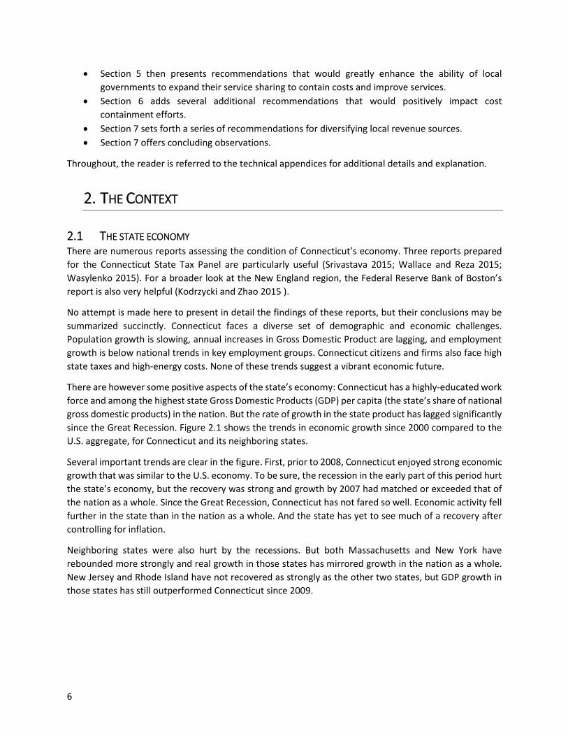
There are however some positive aspects of the state’s economy: Connecticut has a highly-educated work force and among the highest state Gross Domestic Products (GDP) per capita (the state’s share of national gross domestic products) in the nation. But the rate of growth in the state product has lagged significantly since the Great Recession. Figure 2.1 shows the trends in economic growth since 2000 compared to the U.S. aggregate, for Connecticut and its neighboring states.

Several important trends are clear in the figure. First, prior to 2008, Connecticut enjoyed strong economic growth that was similar to the U.S. economy. To be sure, the recession in the early part of this period hurt the state’s economy, but the recovery was strong and growth by 2007 had matched or exceeded that of the nation as a whole. Since the Great Recession, Connecticut has not fared so well. Economic activity fell further in the state than in the nation as a whole. And the state has yet to see much of a recovery after controlling for inflation.

Neighboring states were also hurt by the recessions. But both Massachusetts and New York have rebounded more strongly and real growth in those states has mirrored growth in the nation as a whole. New Jersey and Rhode Island have not recovered as strongly as the other two states, but GDP growth in those states has still outperformed Connecticut since 2009.

7

Figure 2.1: Economic growth in Connecticut and neighboring states: 2000-2015 (Adjusted for inflation)

Source: U.S. Bureau of Economic Analysis

8

As large as the impact of the Great Recession on Connecticut’s economy has been, it would be a mistake to attribute all the state’s economic challenges to that very significant national event. Figure 2.2 makes this clear. The figure reports total earnings per employed person for Connecticut and three neighboring states, as a percentage of the national average. Earnings in this case includes the U.S. Bureau of Economic Analysis statistics for:

• Wages and salaries • Supplements to wages and salaries for employer contributions for pensions, insurance, and

government social insurance programs • Proprietor’s income

This total was then divided by total employment to arrive at the earnings per employed person.

Figure 2.2: Earnings per employed person as a percent of the national average: 2000-2015

Source: U.S. Bureau of Economic Analysis

Several key observations should be noted from the trends depicted in the figure.

• Earnings per employed person in four of the states are well above the national average. Workers in Connecticut and three of its neighboring states enjoy comparatively high compensation levels, and this was true even during the Great Recession.

90%

95%

100%

105%

110%

115%

120%

125%

130%

135%

140%

145%

2000 2001 2002 2003 2004 2005 2006 2007 2008 2009 2010 2011 2012 2013 2014 2015

Perc

ent o

f Nat

iona

l Ave

rage

Connecticut Massachusetts New Jersey New York Rhode Island

9

• Connecticut’s workers saw earnings gains between 2006 and 2009 that were significantly larger than the nation as a whole, and much higher than in neighboring states. And when incomes fell in 2009, they did not fall as much in Connecticut as in the nation as a whole.

• But the overall trend for Connecticut, New York and New Jersey has been downward sloping over this 16-year period. Between 2000 and 2002, earnings per employed person in Connecticut were about 30 percent higher than the national average. By 2015, the figure had dropped to less than 25 percent higher. Similar relative declines occurred in both New York and New Jersey. Among these states, Massachusetts alone has largely been able to avoid this downward trend.

• The trend in Connecticut has been particularly painful because the strong relative gains and smaller losses between 2006 and 2009 were followed by a relatively rapid return to the longer-term trend as the rest of the nation recovered from the recession.

For a more detailed description of the state economy, see Appendix B.

The conclusion is unavoidable. Connecticut has a strong economic base and a well-compensated work force compared to the rest of the nation. But the lack of economic growth in recent years and earnings that are not increasing at the same rate as the rest of the nation mean that Connecticut cannot continue to rely on public spending and revenue policies that may have worked well in the past but do not match the current economic realities.

2.2 THE STATE BUDGET There are many reports and studies documenting the condition of the Connecticut state budget. For purposes of the analysis presented here, two trends serve to make the central point.

First, the U.S. Bureau of Economic Analysis data indicate that between 2006 and 2015, the state economy grew by 17 percent. During that same period, spending by Connecticut state government grew by 48.9 percent, or 2.9 times faster than the state economy.

Second, as is shown in Figure 2.3, the Connecticut Comprehensive Annual Financial Report which details the aggregate state revenues and expenditures for the past ten years, shows that state expenditures have exceeded state revenues every year since 2007. As indicated in the introduction, this trend is likely to continue for several more years.

The ability of Connecticut state government to provide state aid to local governments has seriously eroded over the past decade. And the state has repeatedly demonstrated a willingness to divert resources intended for local governments to fill perceived needs at the state level.

The condition of the state economy and the challenges facing Connecticut state government combine to support the argument that it is now time to revisit both the size and the funding structure for governments in Connecticut.

10

Figure 2.3: Connecticut state revenues and expenditures: 2006-2015

Source: Connecticut Comprehensive Annual Financial Report: Fiscal Year Ended June 30, 2015 (http://www.osc.ct.gov/2015cafr/cafr2015.pdf)

3. THE NEED FOR REVENUE DIVERSIFICATION IN CONNECTICUT

3.1 “CONNECTICUT IS A HIGH TAX STATE” Taxes in Connecticut are widely perceived to be very high. Figure 3.1 reports recent data that appears to support this view. The data shown is the total state and local government taxes per capita for selected states for the 2014 fiscal year (the most current national data available). As shown in the figure, Connecticut ranks 5th among states in total state and local taxes per capita and is 55 percent higher than the national average for 2014. Property taxes per capita in Connecticut ranked 4th highest in the nation and were 90 percent above the national average.

Connecticut’s immediate neighbors also rank relatively high in taxes per capita. Massachusetts, Rhode Island, New York and New Jersey all rank among the top ten states in property tax per capita, and only Rhode Island drops out of the top ten in total state and local taxes per capita. Additional detail, including the actual revenue per capita for all states, is reported in Appendix D, table D.1 for total state and local taxes per capita and table D.2 for property taxes per capita.

11

Figure 3.1: Connecticut taxes per capita compared to other states: 2014a

a. Numbers above the bars are the national rank of each state Source: U.S. Census, State and Local Government Finance

Connecticut is a comparatively wealthy state and it may be that measuring taxes per capita does not adequately reflect the capacity of Connecticut residents to pay for public services. By Federal law, the U.S. Department of the Treasury is required to estimate the relative fiscal capacity of each state each year.1 The measure produced is called Total Taxable Resources and is used in selected Federal program allocations to states. It also provides a reasonable base for comparing tax burdens across states.

Figure 3.2 shows Connecticut’s total state and local taxes, and the property tax, as a percentage of Total Taxable Resources and compares Connecticut to both the U.S. average and other states. Here again, Connecticut’s tax level appears to be relatively high. Connecticut ranked 8th among all states in both total taxes and the property tax. State and local governments were 13% above the national average in total taxes and the property tax was 38% above the national average. Again, additional details and more states are reported in Appendix D, tables D.1 and D.2.

1 Public Law 102-321. For further details, see https://www.treasury.gov/resource-center/economic-policy/taxable-resources/Pages/Total-Taxable-Resources.aspx.

5

76

3

15

47

13 11

35 39

2718

4

9

26

8

30

11

17 2740

29 22

$0

$1,000

$2,000

$3,000

$4,000

$5,000

$6,000

$7,000

$8,000

$9,000

Dolla

rs p

er c

apita

: 201

4

All State & Local Taxes Property Tax

12

Figure 3.2: Connecticut taxes as a percent of Total Taxable Resources (TTR) compared to other states: 2014a

a. Numbers above the bars are the national rank of each state Source: U.S. Census, State and Local Government Finance; U.S. Department of the Treasury

One other perspective clarifies the relative level of the property tax in Connecticut compared to other states. There is no question that Connecticut has some of the wealthiest households in the nation. This disparity in relative wealth shows up most prominently in the personal income tax. In the 2014 tax year, nearly 67 percent of all Connecticut tax returns reported a Federal Adjusted Gross Income (AGI) of $74,000 or less. These taxpayers collectively paid only 10.5 percent of the state income tax collected that year.2 Connecticut’s progressive income tax is not unusual, but it does point out the need to consider how the property tax incidence may differ for more moderate income households.

It is difficult to obtain detailed estimates of the incidence of the property tax by income. Renter occupied housing is subject to the property tax, but it is not clear how much is born by the owner and how much is paid by the occupant. It is also difficult to obtain detailed distributions by state. The U.S. Census Bureau’s American Community Survey provides probably the best cross-state comparisons for owner-occupied

2 Connecticut Department of Revenue Services, http://www.ct.gov/drs/cwp/view.asp?a=1445&Q=545762&PM=1

8

31

14

6

17

42

12

2633

3630

23

8

15

4

105

22

11

3316

4029 24

0%

1%

2%

3%

4%

5%

6%

7%

8%

9%

10%

Perc

ent o

f Tot

al T

axab

le R

esou

rces

All State & Local Taxes Property Tax

13

housing. The comparisons reported here are based on survey results for owner-occupied housing between 2011 and 2015, with all dollar values updated to 2015 levels.

Figure 3.3 reports the median real estate taxes paid by owner-occupied households, divided by the median household income of such households. More detailed data is available in Appendix D, table D.3. This measure is akin to the commonly used housing affordability index which calculates the cost of the median home as a percentage of median household income. The ratio reported in Figure 3.3 and detailed in Appendix D makes the point quite clearly that the property tax in Connecticut is a more significant burden for middle income families in Connecticut than in all but two other states.

Figure 3.3: Median Real Estate Tax as a Percent of Median Household Income: Owner-Occupied Housinga

a. Numbers above the bars are the national rank of each state Source: U.S. Census Bureau, American Community Survey

An analysis carried out by the Connecticut Department of Revenue Services concluded that the property tax in Connecticut is regressive, meaning that lower income households pay a higher percentage of their income for property taxes than do wealthier households. (Sullivan 2014; Bell 2015) The same study found that the 1.176 million residential properties in Connecticut generated $7.32 billion in property tax revenue, or an average of $6,217 per property.

3

9

1

4

7

23

6

1916

30

20

11

0.0%

1.0%

2.0%

3.0%

4.0%

5.0%

6.0%

7.0%

8.0%

9.0%

Perc

ent o

f med

ian

hous

ehol

d in

com

e fo

r ow

ner-

occu

pied

ho

usin

g

14

The impact of residential property taxes on economic development cannot be discounted. Corporations considering locating or expanding in Connecticut must also recruit and retain employees. The challenge of attracting and retaining highly qualified workers is made more difficult when those families will face property taxes that are over twice the national average. The recent State Tax Panel also concluded that the property tax in Connecticut is regressive and that it has a detrimental impact on economic development. (Connecticut Tax Panel 2015)

Acknowledging that taxes, and especially property taxes, are high in Connecticut compared to other states is not new or particularly informative unless answers are provided for the related question of why. There are at least four potential reasons why property taxes in Connecticut may be so much higher than in other states.

• Local governments may be comparatively larger and do more than elsewhere • Unit costs in Connecticut, especially for labor, may be higher than in other states • Alternative revenue sources employed in other states may not be available to Connecticut local

governments • Local governments may be less efficient than in other states

Each of these possibilities is explored before turning to a set of recommendations for change and improvement.

3.2 ARE CONNECTICUT LOCAL GOVERNMENTS LARGER THAN IN OTHER STATES? The size of government can be assessed from multiple perspectives. In virtually all governments, the largest single expense is personnel, and the public sector competes with the private sector for talent and expertise. Thus, a relevant measure of government size is total public sector employment in relation to total private sector employment. A higher percentage implies that government is larger in relation to the private sector.

Table 3.1 reports on state and local government employment as a percentage of total private sector employment for the period 2010 through 2015. State employees are included even though the focus is on local government size because the division of responsibility between state and local government differs across states. Combining the two levels ensures that comparisons across states more reliable. Based on this assessment, state and local government in Connecticut ranked as the 41st smallest in the nation.

Another trend that emerges in the data shown in table 3.1 is that state and local government employment across the nation is shrinking in relation to private sector employment. The national percentage fell from 13.4% in 2010 to 11.9% in 2015. This trend also occurred in Connecticut, though the decline was not as rapid. One result of this more moderate rate of decline is that state and local employment in Connecticut has increased slightly relative to the rest of the nation since 2010. In 2010, state and local employment relative to private sector employment in Connecticut was 90.8% of the national average. By 2015, that ratio had increased to 95.4% of the national average.

15

Table 3.1: State and local government employment as a percentage of total private sector employment

State Percent of Private sector employment Rank 2010 2011 2012 2013 2014 2015 2015

New York 14.2% 13.4% 13.0% 12.7% 12.4% 12.1% 19 Maine 13.1% 12.8% 12.7% 12.5% 12.4% 12.0% 30 U.S. Average 13.4% 12.9% 12.6% 12.3% 12.1% 11.9% New Jersey 13.1% 12.4% 12.2% 12.1% 11.9% 11.5% 36 Connecticut 12.2% 11.8% 11.7% 11.6% 11.5% 11.3% 41 New Hampshire 11.9% 11.6% 11.4% 11.2% 11.2% 10.8% 45 Massachusetts 10.5% 10.3% 10.2% 10.0% 10.0% 9.7% 47 Pennsylvania 10.9% 10.5% 10.1% 10.1% 9.9% 9.6% 48 Florida 11.3% 10.8% 10.4% 10.0% 9.6% 9.3% 49 Source: U.S. Bureau of Economic Analysis

Focusing more narrowly on just local government employment is revealing. Figure 3.4 reports local government employment as a percentage of total private non-farm employment for Connecticut and the national average. As a state, Connecticut has fewer local government employees as a percentage of total private sector employment than the national average. Between 2000 and 2015, Connecticut ranked between 39th and 44th, with a rank in 2015 of 41st. Over the past decade there has been a consistent drop in the relative size of local government employment except during the worst of the recession years.3

Figure 3.4 Local government employment as a percentage of total private non-farm employment

Source: U.S. Bureau of Economic Analysis

3 Another common way to report government employment is in relation to population. Appendix D, table D.4 reports 2015 full- and part-time local government employment per 10,000 population by state. Based on this metric, Connecticut is about 4 percent below the national average and ranks as the 34th smallest in the nation.

5.0%

5.5%

6.0%

6.5%

7.0%

7.5%

8.0%

8.5%

2000 2002 2004 2006 2008 2010 2012 2014

Perc

ent o

f Tot

al E

mpl

oym

ent

United States Connecticut

16

Of course, the number of employees is not the only reasonable measure of relative government size. Connecticut is an expensive labor market, and the cost per employee could be quite a bit higher than in other states. In addition, other non-employee costs could drive up the total cost of government. A second approach to assessing the relative size of government recognizes that governments require financial resources to operate. Size can therefore be measured in relation to the capacity of a state to fund government services. In this case, the metric used is total general government expenditures in relation to the U.S. Treasury Department’s measure of total taxable resources4 in each state. Here again, a higher percentage implies that government is larger in relation to the economy, without suggesting a negative connotation.

Figure 3.5 reports the data for the most recently available cross-state government expenditure data, FY 2014. The percentages in the figure report total local government general expenditures5 as a percent of total taxable resources in FY 2014. Also shown are the rankings for local non-education spending and local elementary and secondary education spending. More detailed data, including data for state spending, are included in Appendix D, table D.5. In the comparison shown in the figure, Connecticut local governments as a group rank 50th out of 50 states and the District of Columbia as having the lowest cost of local government, excluding public education. (Delaware has a smaller local government sector, but when combined with state spending, Delaware ranks well above Connecticut. See Appendix D.)

Figure 3.5: Local General Government Expenditures as a Percentage of Total Taxable Resources: 2014a

a. Numbers above the bars are the national rank of each state Source: U.S. Department of Treasury, U.S. Census Bureau and author calculations

4 See note #1 above. 5 General government expenditures include current expenditures for education, libraries, public welfare, hospitals, health, employment security administration, veteran’s services, transportation, public safety, environment and housing (including parks and recreation), and governmental administration. Excluded are capital outlays, interest on general debt, miscellaneous commercial activities, and utilities.

50 4842

9

43

6

2331

17

5

162725

42

13 8 9

4323

3220

47

18 14

0.0%

0.5%

1.0%

1.5%

2.0%

2.5%

3.0%

3.5%

4.0%

4.5%

Perc

ent o

f Tot

al T

axab

le R

esou

rces

Local Non-education Local Elem. & Sec. Education

17

As a percentage of Total Taxable Resources, elementary and secondary education spending by local governments in Connecticut ranks about in the middle of all states at 25th, just slightly higher than the national average. Current education spending in Connecticut represented two-thirds of total local government expenditures in 2014, which ranked as the 3rd highest percentage among all states.

The comparisons depicted in Figure 3.5 and Appendix D confirm the comparisons based solely on government employment reported earlier. Compared to other states, Connecticut local governments represent a relatively small share of total state employment and place a comparatively small claim on the taxable resources in the state.

3.3 ARE CONNECTICUT PUBLIC SECTOR LABOR COSTS HIGHER THAN IN OTHER STATES? The size of government in Connecticut cannot explain why taxes in Connecticut, especially property taxes, are higher than in other states. Connecticut governments as a group, especially local governments, are much smaller than in nearly all other states.

On the other hand, Connecticut compensation levels per local government employee have been higher than the national average, ranking between 6 and 10 nationally. The state was ranked 10th in 2015. But Connecticut local governments must compete with other sectors to attract and retain talent. And Connecticut is a high compensation state, ranking between 3rd and 5th in the nation since 2000 (see Appendix B). In order to obtain an accurate comparative understanding of local government labor costs, it is essential to adjust for broader labor market conditions that exist in the state.

Figure 3.6 reports the compensation per local government employee as a percentage of the national average, after adjusting for variations in state labor market conditions. Local government employee compensation in Connecticut is on a par with Massachusetts, and is slightly below the national average and other neighboring states once state labor market conditions are factored in.

Figure 3.6: Compensation per local government employee as a percent of National Average, adjusted for state labor market

Source: U.S. Bureau of Economic Analysis and author calculations

75%

80%

85%

90%

95%

100%

105%

110%

115%

120%

125%

130%

2000 2001 2002 2003 2004 2005 2006 2007 2008 2009 2010 2011 2012 2013 2014 2015

Perc

ent o

f Nat

iona

l Ave

rage

Connecticut Massachusetts New Jersey New York Rhode Island

18

Thus, while Connecticut’s relatively high compensation levels may account for some of the need for higher taxes, they do not tell the full story.

3.4 ARE CONNECTICUT LOCAL GOVERNMENTS USING THE FULL RANGE OF POTENTIAL REVENUE

SOURCES? Taken as a group, state and local governments receive nearly all of their general revenue from one of three sources:

• Taxes imposed within the state, either by the state or by local governments • Charges and fees assessed by state and local governments for specific services • Payments from the Federal government

General revenues include all those revenues that are not dedicated to a specific purpose in advance, such as utility fees or other business-type government activities. The charges and fees included in general revenues are those associated with activities funded through the General Fund such as dog licenses, building permits, business licenses, inspection fees, etc.

States differ so markedly in the structure of local revenues that comparing Connecticut to the national average provides little insight. For example, not all states have a sales tax (five do not), nor do all have a state personal income tax (seven do not). The national average would conclude that all states have both an income tax and a sales tax.

It is very insightful though to compare Connecticut to other states which generate roughly the same amount of local government general revenue per capita. In 2014, local governments in Connecticut received $4,539 per capita, based on U.S. Census data. Eleven other states also received between $4,230 and $4,790 per capita that same year. Connecticut led the nation in the percentage of local government revenue generated through the property tax at 61.2 percent. For the eleven other states with similar total general revenue per capita, the property tax represented on average only 33.5 percent of total general revenue. Table 3.2 reports where these eleven other states obtained the rest of their general revenue and compares their experience to Connecticut’s.

• Federal payments: Ten of the eleven states received a higher percentage of their revenue from Federal programs than did Connecticut. The average for these ten was 4.8% compared to Connecticut’s 3.5 percent.

• State payments: Nine of the eleven states received a higher percentage of their revenue from their state government than did Connecticut. In the aggregate, local governments in Connecticut received 27.3 percent of their general revenue from state programs. As mentioned earlier and discussed more fully in Appendix D, this percentage has been declining in recent years, and the trend seems likely to continue. In contrast, the nine states with higher relative levels of state aid received on average 36.8% of their general revenue from state governments.

• General sales tax: Connecticut municipalities do not have direct access to the general sales tax, but nine of the eleven states shown in the table do. In Colorado, the general sales tax generates nearly 14 percent of total general revenue. The average for the nine states is 4.5% of general revenue. Massachusetts and Maryland are the exceptions to this pattern.

19

• Selective sales tax: Selective sales taxes are targeted on specific goods and services such as motor fuel, alcoholic beverages, tobacco and especially public utilities. Connecticut does not currently allow local governments to assess such taxes, but all eleven of the states listed do. The level of the tax varies from a modest 0.4 percent of revenue in Wisconsin, to over four percent in Washington and Illinois. The average is 1.9 percent of total general revenue.

• Individual and corporate income taxes: Only a handful of states employ a local tax on personal or corporate income. Among the eleven states listed, only Iowa, Maryland and Pennsylvania have a local personal income tax, and only Pennsylvania reports revenue from a local corporate income tax.

• Motor vehicle and other taxes: Nine of the eleven states report other tax revenues that total more than is received by Connecticut local governments as a percent of total revenue. These are generally small “boutique” taxes, but it is noteworthy that on average they generate over two percent of total general revenue.

• Current charges: All eleven states place much greater reliance on current charges and fees than do local governments in Connecticut, and by substantial percentages. On average, the local governments in these states place over twice the reliance on charges and fees compared to Connecticut, receiving 17.2 percent of their general revenue from charges, compared to 7.2 percent in Connecticut.

Overall, if Connecticut municipalities matched the average reliance levels exhibited in these eleven states for these revenue sources, excluding personal and corporate income taxes, the need for property tax revenue could be reduced by over 46 percent. Total local government revenue would remain unchanged, though there would likely be some degree of redistribution among municipalities.

The findings thus far indicate that while taxes, and especially the property tax, are high in Connecticut, local governments are comparatively small, especially if public education is excluded. It is true that labor costs are relatively high, but not out of step with broader labor market conditions. The major factor underlying high property tax rates is that local governments are unable to diversify their revenue sources by employing fiscal tools that are in common use throughout the country.

What has yet to be discussed is the issue of efficiency in service delivery. The next three sections of this report discuss both present efforts to enhance service efficiency through shared services, and the policy and practice changes that are needed to allow local leaders to pursue greater cost savings through creative and collaborative interlocal efforts.

20

Table 3.2: Local government general revenue by source for selected states: 2014

State

Percent of general revenue by source Revenue

per capita

Federal payments

State payments

Property tax

General sales tax

Selective sales tax

Individual income tax

Corporate income tax

Motor vehicle &

other taxes

Current charges

Connecticut 3.5 27.3 61.2 0 0 0 0 0.9 7.2 4,539 Colorado 4.9 25.2 29.9 13.9 1.6 0 0 2.0 22.5 4,577 Illinois 5.7 30.7 42.3 2.5 4.5 0 0 1.4 13.0 4,743 Iowa 3.6 35.0 33.2 2.1 1.7 0.8 0 0.6 23.1 4,600 Maryland 4.9 28.5 30.4 0 3.1 17.7 0 2.8 12.5 4,512 Massachusetts 5.0 30.7 51.6 0 1.2 0 0 1.1 10.4 4,231 Minnesota 3.6 45.7 27.3 1.0 0.7 0 0 1.0 20.7 4,605 Nebraska 4.0 25.4 38.1 4.0 1.9 0 0 5.5 21.1 4,616 North Dakota 6.7 49.1 23.7 5.7 0.7 0 0 1.2 12.9 4,720 Pennsylvania 4.3 35.9 31.8 1.2 1.1 8.5 0.8 2.7 13.5 4,404 Washington 5.0 32.6 22.7 8.5 4.1 0 0 2.5 24.7 4,784 Wisconsin 2.4 43.1 37.6 1.4 0.4 0 0 0.8 14.3 4,331 Number of states > Connecticut 10 9 0 9 11 3 1 9 11

Average of states > Connecticut

4.8 36.8 4.5 1.9 2.1 17.2

Source: U.S. Census Bureau, State and Local Finance and calculations by the author

21

4.0 COLLABORATION AND SERVICE SHARING: CURRENT One approach to improving efficiency, containing costs and improving service quality is through interlocal collaboration and service sharing. Some required or desired services are difficult to deliver efficiently by a single municipality because the availability of the required technical expertise is limited. In other cases, the level of service demand may be low enough that either the quality of service provided is low, or the necessary capital and labor costs to meet the demand result in excess capacity for a single jurisdiction. Good management of public resources may argue for improved efficiency or enhanced service quality through sharing of services with other public entities.

There are numerous examples of such service sharing across local governments in Connecticut. Many of these efforts are documented elsewhere. For the most part, these efforts fall into one of three categories:

• Interlocal efforts sponsored and supported by one or more Councils of Governments • Interlocal agreements between two or more local governments • Informal sharing arrangements initiated through professional contacts and relationships

In addition, there are often parallel efforts to share services across school districts, and between a school district and the town it serves.

Not all service sharing efforts have been successful at reducing costs or improving services. But the many efforts demonstrate that there is both a recognition that service sharing is viable and needed, and a demonstrated willingness on the part of local officials to consider, experiment, and implement service sharing arrangements.

Interlocal cooperation at the Council of Governments level is actively being promoted and achieved across the state. In 2015, the Connecticut Conference of Municipalities published Innovative Ideas: Regional cooperation for a more viable Connecticut. (CCM 2015) The report highlights current service sharing on a number of fronts. Examples include:

• Eight members of the River COG have joined to form the “Gateway Commission” to protect the environmental and scenic resources and enhance the economic potential of the Lower Connecticut River Valley.

• Municipal Services are being provided or facilitated by the Capitol Region Council of Governments (CRCOG), including

o Purchasing Council o Natural Gas Consortium o Electricity Consortium

• The CRCOG is also promoting a Connecticut e-Government Initiative that includes o Regional Online Permitting o Fiber Infrastructure o General IT Services o CRCOG Data Center

Other regional examples include CRCOG’s Geographic Information System which serves 38 towns, regional election monitoring, and regional solid waste management. In the Naugatuck Valley COG, the

22

Naugatuck Valley Regional Brownfields Partnership has expanded to include 27 cities and towns in west central Connecticut.

Initiatives also span multiple regions in efforts such as the Nutmeg Service Cloud which is a cloud server and high speed broadband service used by 97 municipalities, public safety entities, schools, and libraries in the state.

At the municipal level, the CCM report lists cooperative arrangements in energy, health insurance, economic development, public safety, environmental preservation, equipment sharing, property revaluation, senior and youth services, public health, and regional trails.

On a more informal level, the River COG has successfully facilitated the Regional Land Trust Exchange, an association of thirteen land trusts in the region and the town of Salem. This informal organization provides shared services for member conservation commissions, the town and particularly their land trusts.

There are also numerous examples of service sharing among Connecticut’s school districts. The Connecticut Association of School Business Officials (CASB) recently released a white paper describing many current efforts to share services with towns and across school districts. The report also notes both challenges and additional opportunities for further increasing sharing. (CASB 2015)

But the opportunities for increased cooperation and service sharing across the state are hindered by both policies and practices. The next section identifies specific recommendations for change that would significantly increase the level of service sharing in the state.

5.0 PROPOSALS FOR EXPANDING SHARED SERVICES AND COLLABORATION The policy impediments to further service sharing efforts can be grouped into three general areas:

• Employment practices • Town charter restrictions • State government practices

Four additional specific recommendations are made here. In combination, these recommendations will significantly alter the landscape for shared services within the state. Not all towns and cities will pursue all the options implied in these recommendations. But overall, the increased flexibility and support will strongly encourage local innovation and initiative.

5.1 PROPOSED CHANGES IN MUNICIPAL EMPLOYEES RELATIONS ACT (MERA) Some of the challenges frequently encountered when towns seek to pursue shared services are the limitations imposed by existing collective bargaining agreements. Connecticut General Statutes Section 7-478a(c), which addresses interlocal agreements, states:

“A decision by a municipal employer to enter into or implement an interlocal agreement under sections 7-339a to 7-339l. inclusive, shall not be a subject of collective bargaining…”.

We recommend that similar language be adopted regarding service sharing more broadly as follows:

23

• The decision to reassign or subcontract bargaining unit work as a consequence of interlocal sharing of such services shall not be a subject of collective bargaining.

In addition, we recommend that state law be changed to ensure that:

• In all future collective bargaining agreements, municipalities cannot bargain away, or be required through arbitration to give up, their right to assign employees to carry out their normal responsibilities in a new location or to provide services to a different municipality.

• When service sharing arrangements affect two or more collective bargaining units, the interests of all employees affected by the new arrangements will be represented by either a coalition of bargaining units or a new bargaining unit will be created to represent all affected employees.

5.2 CHARTER CHANGES Another set of constraints encountered by some towns is that town charters were crafted in a period when flexible delivery of services was not as essential as it is today. Charter restrictions and town ordinances have limited some towns’ abilities to pursue significant restructuring and cooperative arrangements. We recommend that state law be changed so that interlocal agreements or service sharing contracts involving two or more municipalities will override any participating municipality’s relevant charter sections and ordinances.

Further, efforts should be made to modify charters and eliminate references to specific organizational structures including departments. Charter sections should focus on the services desired, not the organizational structure needed to deliver those services.

5.3 STATE PRACTICES While many provisions in state law would seem to promote interlocal cooperation and agreements to promote service sharing, there are also key state policies and practices that serve to limit and discourage service sharing. We recommend that the state:

• Restore funding for the Regional Performance Incentive Program and target that funding on initiatives identified as most effective in reducing costs, improving services or containing further cost increases. (see section 5.6)

• Change state budgeting and accounting practices so that revenues identified in law as local government revenues are sequestered and cannot be budgeted or spent for state functions even though they may be initially collected by a state agency.

• Modernize state IT resources and practices by 2020 to facilitate electronic filing of local government reports and communication between state and local agencies.

• Allow municipalities to establish service districts along the lines of the existing health district model to perform and deliver specified municipal or educational services (e.g., special education).

5.4 ADVISORY COMMISSION ON INTERGOVERNMENTAL RELATIONS (ACIR) The state needs an active, state-wide entity to evaluate, facilitate and encourage interlocal service sharing and state-local interactions. In the past, the Advisory Commission on Intergovernmental Relations (ACIR)

24

has filled this role, but the ACIR has not been effective for quite some time. We recommend that ACIR be revitalized, and given two specific charges in the near term:

• In collaboration with CCM, the nine COGs, and the Connecticut Council of Small Towns (COST) identify services that are currently being subsidized by the state and are duplicated within the municipalities, and reduce subsidies accordingly (e.g., non-instructional and “back office” educational functions)

• Review state mandates with the intent to incentivize local governments to aggressively pursue greater efficiency and cost savings by relaxing or modifying selected mandates when cooperative efforts involve two or more municipalities

5.5 STATE LAW RELATED TO Councils OF GOVERNMENT (COGS) Councils of government should play a vital role in both planning and facilitating shared service arrangements, and in delivering services within their region where appropriate. In many instances, a single state-wide approach to service sharing is not appropriate and will need to be adapted to regional needs and capacities. We recommend state law be modified to assure that COGs can effectively fill this role.

• Require COGs to develop plans for region-specific collaboration and/or service sharing. Initially, their efforts should be focused in the following areas:

o 911 (PSAP) call centers including training, service delivery and performance evaluation o Special education services, in collaboration with regional education service centers o Education transportation o Paratransit, dial-a-ride o Library operations o Public health services, including service standards and performance evaluation o Collaborative purchasing (especially among smaller jurisdictions) o Code enforcement functions

• Change state law as needed to expand the range of services that can be offered directly by COGs.

5.6 CONNECTICUT CONFERENCE OF MUNICIPALITIES, COST AND COGS The Connecticut Conference of Municipalities (CCM) should also play a leadership role in developing strategies and promoting interlocal service sharing. We recommend that

• CCM, COST, and the nine COGs should jointly issue a blueprint for promoting and expanding interlocal cooperation, interlocal contracting and expanded service sharing. The endorsement of this blueprint by ACIR should be sought and obtained. (See appendix A)

• CCM, COST, and the COGs should facilitate participation in existing national municipal performance benchmarking efforts or should initiate a regional benchmarking program. The results of the on-going benchmarking should be used to inform the allocation of Regional Performance Incentive Program grants (see section 5.3).

25

5.7 SPECIFIC PROPOSALS In addition to these more general policy recommendations, we recommend four specific service sharing initiatives. Three of the four proposals relate to public education. In light of the recent court rulings and on-going litigation related to the Connecticut Coalition for Justice in Education Funding case, these initiatives should be pursued in the very near term.

• Consolidate and/or share services for selected non-instructional education expenditure categories across school districts.

Table 5.1 reports average expenditures per enrolled student by size of school district for four non-instructional categories. In each case, there is a negative relationship between the size of the district and expenditures per student, especially for districts with fewer than 5,000 enrolled students. This means that larger districts tend to have lower per student costs in at least some areas. Districts with less than 5,000 students enrolled represent 86% of the districts and 51% of enrolled students.

Table 5.1: Selected non-instructional expenditures per student by size of district: 2013-14

Enrolled students, total

2013-14 Expenditures per enrolled student Percent of

districts Percent of

total enrolled Administration & support services

Plant O&M Transportation Other

78-400 2,493 1,918 1,007 284 18% 1% 401-1000 2,071 1,763 962 253 19% 4% 1001-2300 1,780 1,749 986 233 18% 10% 2301-3500 1,638 1,526 875 205 19% 19% 3501-5000 1,516 1,590 936 182 11% 16% 5001-7500 1,636 1,786 833 201 7% 16% 7500-10000 1,480 1,426 739 152 2% 7% 10001-15000 1,578 1,288 862 100 2% 8% 15001-22000 1,770 1,412 919 151 3% 19%

Source: Connecticut Edsight (edsight.ct.gov)

The potential savings in these four categories for districts with fewer than 5,000 students could approach $80 million per year. The argument is not that every district will save money, or even that every district should consolidate their non-instructional operations across current district boundaries. Rather, the data suggests there are strong economies of scale in these service areas that should be explored and every effort made to achieve a more optimal scale of operations.

• Change state law to allow town governments to require consolidation and/or sharing of non-instructional services and resources between school districts and the municipality in which they are located.

There seems to be no compelling reason why the same service capacity should be duplicated in both a municipality and that municipality’s school district. Local officials have the administrative capacity to adjust the scale and scope of operations to serve both entities. State law should not prevent such efficiencies.

26

• The State should assume responsibility for both financing and delivering services for special education.

At present, the needs of the state’s 70,000 special education students are not uniformly met across the state and many districts struggle to provide needed services. State regulations make it extremely difficult for localities to budget and manage special education appropriately from year to year. Students would be better served, and funding would be better utilized, if special education funding were centralized at the state level, and services provided at either the state or regional level. How the state determines to deliver special education services will undoubtedly vary by locality. The key point is that all responsibility for special education should be transferred to the state.

In FY 2014-15, Connecticut school districts spent $1.8 billion on special education. Thirty percent of that total was paid out to either transport pupils (8.3 percent) or to pay for tuition in other schools (21.6 percent).

In that same year, the state sent $2.48 billion to local districts, excluding land, buildings, capital expenditures and debt service. Local districts received an additional $101 million from the Federal government. But the share of special education costs covered by state and Federal aid is highly erratic. Not all state and Federal aid is earmarked for special education. But the comparison of the cost of special education and the amount of external aid received highlights the challenges faced by many districts. Table 5.2 reports the distribution of special education expenditures in districts as a proportion of total state and Federal revenues received.

In the table, 100 percent in the first column implies that the expenditures for special education exactly equaled the total state and Federal assistance received. Values over 100 percent indicate that the local district spent more for special education than the total of all state and Federal assistance received. The maximum observed was 580% in New Canaan, but the percentage was greater than 300% in 24 districts. Over 42 percent of all districts spend more on special education that the total of state and Federal aid received. From a purely financial perspective, education costs would be reduced in these districts if the state kept all state and Federal operating assistance and assumed all costs for special education.

Table 5.2: Special education expenditures as a percent of state and Federal payments received

Special education expenditures as a percentage of total state and

Federal payments received

Percent of school districts

0 to 49% 15.7 50% to 79% 31.3 80% to 99% 10.8 100% to 149% 14.5 150% to 199% 6.6 200% or more 21.1

The state should also adopt the federal standard for burden of proof in special education due process hearings.

27

• Consolidate and/or share assessment services in Connecticut regions for assessment offices servicing less than 15,000 parcels.

Based on a 2013 national study conducted by the International Association of Assessing Officers (IAAO Research Committtee and Walters 2014), the typical property assessment office is responsible for assessing over 50,000 parcels, has a staff of 15.2 full-time employees and an average budget of about $27 per parcel. Municipal assessors, on the other hand, average just under 15,000 parcels, have a staff of 5.8 full-time employees and a budget of nearly $31 per parcel. Based on national survey data, there is every reason to believe there are economies of scale in property assessment, even after controlling for the complexities faced in Connecticut.

Eighty-six Connecticut assessors responded to the national survey referenced above. They indicated that they service between 907 and 34,800 property parcels, with an average of 7,950. Based on the survey responses, over 80 percent of Connecticut assessment offices are candidates for increasing shared services. The limited information available on assessment office budgets makes it difficult to estimate the potential cost savings. But using the national differential of about $5/parcel, the potential savings in Connecticut will be between $5 and $10 million per year statewide.

6.0 COST CONTAINMENT Interlocal service sharing is not the only issue local leaders face in trying to contain increases in the cost of public services. Some of the frustrations may seem minor, others more significant. But as in many organizational endeavors, small factors can accumulate to yield large results, both positively and negatively. The following major and minor recommendations will all support and enhance local leaders’ ability to contain increases in the cost of government.

6.1 ACCOUNTING AND REPORTING PRACTICES • Urge OPM to complete the benchmarking project using the Uniform Chart of Accounts and

standardized public financial reporting.

OPM has recently undertaken an effort to convert local financial data to the Uniform Chart of Accounts, but this effort is incomplete. Transparency, public accountability and good management dictate that all local public entities in the state have access to complete uniform data for both education and non-education expenditures and revenues.

6.2 LABOR RELATIONS Relationships between state agencies, local leaders, and collective bargaining organizations in Connecticut are often strained by outdated labor arrangements and laws. It is time to systematically review and update both the laws and the processes involved.

• Create a labor relations task force to systematically review and recommend updates for Connecticut’s municipal labor laws and dispute resolution processes.

Without waiting for the results of any such systematic review, the state should modify state-mandated municipal compulsory binding arbitration laws by:

28

• Increasing the power of local governing or legislative bodies to reject arbitrated awards by a two-thirds vote, but provide that the contract negotiation is then reset and starts anew in the event of such a rejection – instead of going to a second, final and binding arbitration panel;

• Allowing local governing or legislative bodies to reject stipulated board of education/teacher agreements. (Stipulated agreements are voluntary agreements between boards of education and teachers within the arbitration process that may be incorporated into awards);

• Allowing municipalities to require that collective bargaining negotiations concerning changes to pension, health and welfare benefits be conducted between a municipality and a coalition committee that represents all municipal employees who are members of any designated employee organization, including employees of the BOE; and

• Requiring that grievance arbitration and unfair labor practice awards be issued no later than 60 days following the date post-hearing briefs are filed. (This would establish timelines for the issuance of decisions in cases before both the State Board of Mediation and Arbitration, and the State Board of Labor Relations).

Municipalities also recommend changes in current employee retirement systems. Specifically, the state should amend the Municipal Employee Retirement System (MERS) to establish an additional retirement plan within MERS, for new hires, that would:

• Maintain a defined benefit plan. Such new tier would be modeled after the State’s tier III, which currently exists within the State Employee Retirement System.

• Change the plan for new employees hired after a certain time period to be part of a town plan instead of the existing plan.

• Allow municipalities the option of negotiating a higher contribution rate towards retirement benefits from MERS participants than currently allowed.

6.3 OTHER RECOMMENDED CHANGES TO HELP CONTAIN COSTS • Eliminate the health insurance premium tax on municipalities which is currently a 1.75% tax on

fully insured municipalities. • Limit the requirement for towns to store the possessions of evicted tenants and amend the

provisions of the Uniform Relocation Assistance Act (URAA) to provide municipalities with far greater flexibility and cost protections in satisfying their obligations under the URAA.

• Enact a statutory prohibition on the passage of unfunded or underfunded state mandates affecting municipalities without a 2/3 vote of both chambers of the General Assembly.

7.0 PROPOSALS FOR REVENUE DIVERSIFICATION Expanding shared services and pursuing increased efficiency in local government operations are essential, but insufficient to assure the fiscal stability and integrity of Connecticut local governments. As noted in sections 2 and 3, and Appendix D, local governments are too reliant on the property tax and state transfers. The level of the property tax burden in the state makes further property tax increases very challenging in most jurisdictions. Coupled with the uncertainty around state aid, local governments have no choice but to pursue other local revenue sources.

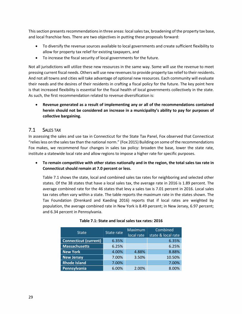
29

This section presents recommendations in three areas: local sales tax, broadening of the property tax base, and local franchise fees. There are two objectives in putting these proposals forward:

• To diversify the revenue sources available to local governments and create sufficient flexibility to allow for property tax relief for existing taxpayers, and

• To increase the fiscal security of local governments for the future.

Not all jurisdictions will utilize these new resources in the same way. Some will use the revenue to meet pressing current fiscal needs. Others will use new revenues to provide property tax relief to their residents. And not all towns and cities will take advantage of optional new resources. Each community will evaluate their needs and the desires of their residents in crafting a fiscal policy for the future. The key point here is that increased flexibility is essential for the fiscal health of local governments collectively in the state. As such, the first recommendation related to revenue diversification is:

• Revenue generated as a result of implementing any or all of the recommendations contained herein should not be considered an increase in a municipality’s ability to pay for purposes of collective bargaining.

7.1 SALES TAX In assessing the sales and use tax in Connecticut for the State Tax Panel, Fox observed that Connecticut “relies less on the sales tax than the national norm.” (Fox 2015) Building on some of the recommendations Fox makes, we recommend four changes in sales tax policy: broaden the base, lower the state rate, institute a statewide local rate and allow regions to impose a higher rate for specific purposes.

• To remain competitive with other states nationally and in the region, the total sales tax rate in Connecticut should remain at 7.0 percent or less.

Table 7.1 shows the state, local and combined sales tax rates for neighboring and selected other states. Of the 38 states that have a local sales tax, the average rate in 2016 is 1.89 percent. The average combined rate for the 46 states that levy a sales tax is 7.01 percent in 2016. Local sales tax rates often vary within a state. The table reports the maximum rate in the states shown. The Tax Foundation (Drenkard and Kaeding 2016) reports that if local rates are weighted by population, the average combined rate in New York is 8.49 percent; in New Jersey, 6.97 percent; and 6.34 percent in Pennsylvania.

Table 7.1: State and local sales tax rates: 2016

State State rate Maximum local rate

Combined state & local rate

Connecticut (current) 6.35% 6.35% Massachusetts 6.25% 6.25% New York 4.00% 4.88% 8.88% New Jersey 7.00% 3.50% 10.50% Rhode Island 7.00% 7.00% Pennsylvania 6.00% 2.00% 8.00%

30

• Reduce the state sales tax rate from the current 6.35 percent to no more than 6 percent.

In 2015, the state collected $3,962 million in sales and use tax at the 6.35 percent rate. Dropping the rate on the current base to 6.00 percent would reduce the revenue to $3,744 million, a reduction of $218 million or 5.5 percent.

• Broaden the sales tax base by repealing existing exemptions for selected consumption categories.

Consistent with recommendations made by Dr. Fox to the State Tax Panel (Fox 2015), we recommend that the Legislature broaden the base for the sales tax by repealing sufficient exemptions to generate an additional $276.1 million for the state while reducing the state rate to no more than 6 percent.

Good tax policy dictates that the state should avoid taxing business inputs, and such exemptions should not be eliminated. However, there are a number final consumption categories that currently represent significant levels of foregone revenue. The Department of Revenue Services produces an annual report on the cost of these exemptions to the state. As an illustration of the revenue potential, Table 7.2 lists some of these categories.

No specific recommendations are made at this time regarding which exemptions should be repealed either fully or partially. CCM recommends a collaborative effort between state and local leaders to identify appropriate exemptions to eliminate or reduce. The point is that in the aggregate, current sales tax exemptions are more than ten times the amount of revenue needed for the state to lower the state rate and still collect the same amount of revenue. Eliminating or reducing exemptions by ten percent ($276.1 million) will more than offset the revenue lost by reducing the state rate.

Table 7.2: Selected Current Sales Tax Exemption Amounts: FY 2014-15

Exemption category Deductions at the 6.35% Tax Rate (millions)

Revenue Potential at 6% (millions)

Aviation Fuel 239.3 14.4 Charitable/Religious – Labor and Services 1,759.1 105.5 Charitable/Religious – Leases and Rentals 59.8 3.6 Charitable/Religious – Sale of Goods 1,315.6 78.9 Electricity ($150 monthly per business) 48.7 2.9 Electricity/Gas/Heating Fuel (residential) 3,381.3 202.9 Electricity/Gas/Heating Fuel for Manufacturing or Agricultural Production 795.3 47.7

Food Products for Human Consumption 6,801.0 408.1 Fuel for Motor Vehicles 7,450.1 447.0 Funeral Expenses up to $2,500 96.0 5.8 Magazines by Subscription and All Newspapers 175.5 10.5 Motor Vehicles Sold to Armed Forces (Difference between the Full and 4.5% Rates) 5.0 0.3

Nonprescription Drugs and Medicines 14.0 0.8 Non-Taxable Labor and Services 16,639.9 998.4

31

Oxygen, Plasma, Prostheses, etc. 210.5 12.6 Pollution Abatement 17.0 1.0 Prescription Medicines 4,554.1 273.2 Purchases of Cigarettes Taxed by a Distributor 665.6 39.9 Renovation Services to Residential Property 475.2 28.5 Sales of College Textbooks 29.2 1.8 Sales Tax Holidays 82.0 4.9 Weatherization Products 123.8 7.4 Water sales 662.7 39.8 Sewer sales 418.3 25.1 Total 46,019.0 2,761.1

Source: Connecticut State Department of Revenue Services; Water and sewer sales are calculated from 2015 annual reports filed with the Connecticut Public Utilities Regulatory Authority and US Census estimates for 2014

• Levy a statewide local sales tax at the rate of 1 percent

With a reduction in the state rate, a local rate of 1 percent would leave the current sales tax rate at the recommended 7 percent or lower, and would generate $670 million annually for local governments (assuming the rate is applied to a broadened base as suggested here).

We recommend that the local sales tax revenue be used first to fully fund the currently unfunded portions of the state property and college/hospital PILOT program as described in the next section. This will require $324 million. The remaining $346 million should be distributed using the current LoCIP formula to allocate funds to towns. The estimated distribution by town is shown in Appendix C.

• With voter approval through consolidated referendum, allow local jurisdictions within a COG to impose a 0.25 percent local sales tax within their COG region to fund recreation, tourism, historic and arts infrastructure and activities of regional significance.

Funds would be collected along with the statewide sales tax and would be remitted by the state to the COG for allocation by the COG Board of Directors. Based on the sales tax by town data employed in Sjoquist (2015), the estimated revenue potential in each COG region would be as shown in table 7.3.

Table 7.3: Estimated annual revenue for 0.25% arts, parks and tourism tax by COG

COG region

Annual revenue from 0.25% regional sales tax

(millions) Current tax base

Capitol $37.0 Greater Bridgeport $8.8 Lower CT River Valley $5.0 Naugatuck Valley $11.0 Northeast CT $1.7 Northwest Hills $3.9 South Central $21.9 Southeastern CT $8.6 Western CT $27.0

32

• With voter approval through consolidated referendum, allow local jurisdictions within a COG to impose a 1 percent local sales tax on food and beverages sold in restaurants, and on hotels within their COG region to fund recreation and tourism infrastructure and activities of regional significance.

The current 15 percent room occupancy tax generated $116.3 million in FY 2014-2015. The U.S. Census Bureau reports that nationally in 2014, food service and drinking place sales (NAICS code 722) were 2.6 times accommodation sales (NAICS code 721).6 The 2012 Economic Census for Connecticut places the Connecticut ratio at 1.9 (food and beverage divided by accommodation). Thus, this one percent tax has the potential to generate between $22 million and $28 million per year statewide. As a local option, actual revenues will depend on which COGs adopt the tax.

7.2 PROPERTY TAX Property tax exemptions seriously erode the property tax base in many towns. Statewide, exemptions represent nearly 12 percent of the aggregated Equalized Net Grand Lists (ENGL). But this statistic seriously understates the issue for some communities. In 11 towns, exempt property, other than city-owned property, represents over 20 percent of the ENGL and in several the total is over 50 percent. While these are the most extreme cases, property tax exemptions affect every town in Connecticut, with the result that the taxes paid by non-exempt taxpayers are higher than they would be without the exemptions.

The challenges for local governments are more extreme because the state has not fully funded PILOT reimbursements. In FY 2015, state reimbursement for private colleges and medical facilities totaled only 30.6% of the tax that would have been due had these properties been fully taxable. And as these institutions acquire additional property, local tax bases are further eroded as taxable property becomes tax exempt.

To reduce the impact of tax exempt properties on local tax bases, we make seven recommendations regarding the property tax.

• Prevent currently taxed property from being added to any of the existing tax exemption categories.

At present, if a tax-exempt organization acquires a property, that property becomes exempt under the new owner’s tax exemption. This proposal would prevent this change in tax status. If a property is currently taxable, it will remain taxable even if acquired by a tax-exempt entity.

• Change state law to require tax exempt organizations to enter PILOT agreements when the entity derives rental or other significant income from a property.

Three states have mandatory PILOT laws for non-profit entities. Delaware, for example, requires non-profit organizations that provide housing for the elderly to pay a fee of “not less than 10% of gross rentals derived from the project,” less certain expenses. (Delaware Code Section 8156)

6 U.S. Census Bureau, Annual Retail Trade Survey

33

Connecticut also requires PILOTs in certain circumstances (See CGS Section 8-265b, Section 12-76 and Section 22a-270a).

The required PILOT payment could be based on either property value, income, or units (e.g., students enrolled). These PILOT agreements should be in force for a period of not less than five years, after which they should be renegotiated and renewed.

• Increase PILOT reimbursements for state-owned property to 77 percent.

With certain exceptions, the statutory reimbursement rate for state-owned property is currently 45 percent, while for colleges and hospitals the statutory rate is 77 percent. But a state-owned office building imposes the same service demands on a municipality as a university-owned office building. Both should be reimbursed at the same rate. Funding for this proposal will be provided by the new local sales tax described previously.

• Consistently and fully fund the state PILOT reimbursement program at the statutory rates.

State government is the entity which determines property tax exemptions, even though the revenue from the property tax is exclusively for local governments. Since every exemption erodes local fiscal strength or increases the tax burden on non-exempt property, the state should consistently and fully reimburse local governments for state exemption choices. Funding to fill the gap between current funding levels and statutorily dictated levels for the PILOT program can be provided through the new local sales tax described previously. See Appendix C.

• Require property owners of properties subject to state PILOT reimbursement to pay the difference between the state’s statutory PILOT rate and the amount towns actually receive in state PILOT payments, up to 20 percent of the mill rate.

If the state is unwilling or unable to fully fund PILOT reimbursements, property owners should be required to make up the difference. An example may help to clarify this proposal. Suppose that a town is the site of a tax-exempt hospital with an assessed value of $100 million, and the town’s mill rate is 30.0. If the hospital were fully taxable, the tax obligation would be $3 million. The state’s statutory obligation is to fund the PILOT for this hospital at 77% of the foregone revenue, or $2.31 million. In 2015, the state funded about 60% of its statutory obligation, or about $1.39 million for the example hospital. Under this proposal, the hospital would be required to make up the shortfall, up to $600,000 (20% of the mill rate). In this example, the shortfall is $917,000, so the hospital would be required to pay the full 20% or $600,000.

The revenue implications of this proposal are difficult to estimate precisely without property-specific information. In the aggregate, the unpaid difference for private colleges and hospitals totals $188 million, based on current mill rates. The estimated additional revenue for towns and cities would total about $81 million per year. Over half of the revenue increment for private colleges and hospitals would be paid in New Haven (34.4%) and Hartford (19.5%). Table 7.4 provides an estimate of the revenue implications for the 30 towns with the largest likely impact from private colleges and hospitals.

34

Table 7.4: Revenue estimates for PILOT shortfall proposal

Town

All values are in millions of dollars except for mill rates Assessed value

of private colleges and

hospitals (2013)

Mill rate

Foregone tax

revenue

Statutory state PILOT

Actual state PILOT

Shortfall

Estimate of PILOT due

from property owners

New Haven 3,350.9 41.6 139.2 107.2 43.5 63.7 27.8 Hartford 1,061.8 74.3 78.9 60.7 25.3 35.5 15.8 Bridgeport 595.3 42.2 25.1 19.3 8.0 11.4 5.0 Middletown 578.1 32.6 18.8 14.5 4.1 10.4 3.8 Waterbury 317.5 58.2 18.5 14.2 5.8 8.5 3.7 New London 353.2 39.5 13.9 10.7 5.0 5.7 2.8 Norwalk 353.3 25.4 9.0 6.9 1.6 5.3 1.8 New Britain 201.4 49.0 9.9 7.6 2.7 4.9 2.0 Hamden 241.5 40.9 9.9 7.6 3.0 4.6 2.0 Fairfield 344.3 24.8 8.5 6.6 2.6 3.9 1.7 West Haven 351.2 31.3 11.0 8.5 5.5 3.0 2.2 Stamford 247.0 25.4 6.3 4.8 2.0 2.9 1.3 Meriden 130.8 36.6 4.8 3.7 1.3 2.4 1.0 Danbury 168.2 28.3 4.8 3.7 1.3 2.3 1.0 Wallingford 125.4 27.5 3.4 2.7 0.4 2.3 0.7 Norwich 93.3 40.9 3.8 2.9 0.8 2.1 0.8 East Hartford 73.0 45.9 3.3 2.6 0.5 2.1 0.7

West Hartford 92.6 38.3 3.5 2.7 1.1 1.6 0.7

Greenwich 262.1 11.3 3.0 2.3 0.9 1.4 0.6 Manchester 73.0 39.4 2.9 2.2 0.9 1.3 0.6 Newington 101.6 35.8 3.6 2.8 1.6 1.2 0.7 Derby 78.4 35.7 2.8 2.2 0.9 1.3 0.6 North Haven

72.5 29.4 2.1 1.6 0.6 1.0 0.4

Bristol 53.9 34.6 1.9 1.4 0.6 0.9 0.4 Windham 56.8 34.4 2.0 1.5 0.7 0.8 0.4 Milford 53.7 27.9 1.5 1.2 0.4 0.7 0.3 Torrington 24.6 45.8 1.1 0.9 0.3 0.6 0.2 Vernon 29.7 36.9 1.1 0.8 0.3 0.5 0.2 Orange 31.1 31.4 1.0 0.8 0.2 0.5 0.2 Stafford 26.4 33.4 0.9 0.7 0.2 0.5 0.2

Source: Connecticut OPM and author calculations

• Include quasi-state properties in the PILOT reimbursement program for state-owned properties.

Under current law, the state has an obligation to make PILOT payments for all state-owned property, Indian reservation land, and municipally-owned airports. (Pinho 2015) The current

35

funding level is about 24% of the statutory level. But there are several other classes of exempt property that are owned by quasi-state entities that are not covered under current PILOT statutes. Table 7.5 lists selected examples of exempt property categories that should be included in the PILOT program for state-owned properties.

Table 7.5 Proposed expansion of the PILOT for state-owned property

Code Description Assessed value (millions)

DBAX Property used for scientific purposes $290.4 DDAX Property used for historical purposes $211.8 RAAX Connecticut Resource Recovery Authority $191.2 SAAX, SAHX Connecticut Housing Authority $113.5 Total $806.8 Source: Connecticut OPM and author calculations

Hartford in particular will benefit meaningfully by adding nearly $200 million in Housing Authority and Resource Recovery Authority property to the state PILOT program. At current funding levels, making this change in the PILOT base will generate between $2 and $4 million per year for Hartford, depending on the mill rate applied to Housing Authority property.

• Require entities exempt from the property tax (e.g., group homes) to pay for specific municipal services, or Service-in-Lieu-of-Taxes (SILOTs) payments to provide for utilities and other non-education related services.

The required SILOT fee could either be some share of specific expenditure categories (e.g., police and fire), or it could be the equivalent of a reduced mill rate (e.g., excluding education) applied to property value.

An example may help to clarify how this proposal would be implemented. Consider a hypothetical recreational property in West Hartford valued at $30 million but currently tax exempt. In 2014, 42.2 percent of West Hartford’s general fund expenditures went for non-educational functions, with the remaining 57.8 percent going to education:

¾ General government (12.8%) ¾ Public safety (10.8%) ¾ Public works (9.7%) ¾ Health and welfare (1.2%) ¾ Culture and recreation (1.3%) ¾ Debt service (6.2%)

In that same year, West Hartford’s mill rate was 23.79. The SILOT program would calculate the fee due by subtracting the share of the mill rate going to education (57.8 percent), and applying the remaining mill rate to the taxable value of the property to arrive at the SILOT payment due:

¾ $30 million X (23.79*.422)/1000 = $300,827.

36

• Review and update all property tax exemptions.

In total, real and personal property tax exemptions total over $62 billion in taxable value statewide, ranging from properties owned by hospitals to manufacturing machinery and equipment. The taxes for some that would otherwise be due are partially reimbursed to towns through PILOT programs. But the exemptions and incomplete PILOT reimbursements impact towns’ capacity to raise the revenue needed to provide services residents desire. For example, the elimination of the PILOT for manufacturing machinery and equipment (PILOT MME), while keeping the exemption mandate, has reduced that capacity significantly in a number of towns.

All of these exemptions should be regularly reviewed to assure that the intended benefits are in fact occurring. The policy options discussed by Dr. Michael Bell in his article for the State Tax Panel should be carefully considered and followed where appropriate. (Bell 2015)

7.3 FEES FOR USE OF THE PUBLIC RIGHT-OF-WAY In a market economy, the right to install and maintain a company’s infrastructure on private land requires obtaining an easement from the land owner, and would in virtually all cases involve some form of compensation to the land owner for that easement. Granting the easement limits how the land can be used in the future and therefore potentially reduces the value of the land. Such easements can be priced using standard appraisal methods. Companies routinely expect to pay for the factors they use in producing their products. An easement across private land is simply another factor in the production process. (Malone 2003) Granting an easement to use a public right of way should be viewed in the same way.

The privilege to place utility infrastructure in a public right of way adds significant value to the entity seeking the easement and limits future uses of the public’s land. Towns and cities should be allowed to require compensation for these privileges. Such compensation is often called a franchise fee. Whatever the name, the compensation differs from a tax in that it is very explicitly a fee for service. In this case, the service is the granting of a right to place private assets in a public right of way.

Connecticut is one of only seven states that does not allow local governments to collect fees for the use of public rights-of-way. While the national average for such fees is about 2.2 percent of total local tax revenue, in some states (e.g., Florida), these fees exceed 6 percent of local tax revenue.

Towns in Connecticut need the option of assessing these fees and obtaining compensation for the use of their valuable assets.

• Change state law and permit municipalities to require on-going fees for the use of the public rights of way.

Many localities charge a fee to utility companies for the privilege of placing company infrastructure in the public right of way. Such fees are commonly charged for electricity, natural gas, telephone, water, sewer, and cable TV, whether privately or publicly owned. These fees typically cannot be charged for fiber optic or other internet infrastructure due to Federal restrictions.

One of the strong advantages of a franchise fee is that all utility customers are required to pay the fee, including government agencies and nonprofit entities.

37

Fees are typically assessed as a percentage of gross receipts and are added as a separate line on the final customer’s bill. Table 7.6 illustrates a 2 percent fee assessed on electric utilities in Connecticut for residential and commercial customers. For all electric sales in the state, a 2 percent franchise fee would yield $43.2 million, based on 2014 revenues.

Table 7.6: Right of way compensation example

Customer class 2014 Average Annual Bill

2% Franchise Fee

Total statewide revenue ($1,000s)

Residential $1,572 $31 $29,262 Commercial $38,733 $775 $11,290

It is difficult to estimate the revenue implications of a franchise fee by municipality. Not all residents in all municipalities have access to natural gas, piped water, or central sewer systems. Using regional statistics on household consumer spending for electricity, natural gas, telephone, and water, along with data from utility companies on communities served and number of customers, it is possible to create some rough revenue estimates. Considering only electricity, natural gas, telephone and water sales, it appears that a 2 percent franchise fee would generate about $72.4 million annually in new revenue.

There is nothing dictating a 2 percent rate. In fact, many jurisdictions in other states charge different rates for different utilities. Thus, the fee may be 4 percent for electricity, but 2 percent for telephone and 6 percent for water. The 2 percent rate used here is purely for illustration. Further, if the imposition of a franchise fee is optional for local governments, not all will choose to implement it. In general, it will be the larger communities that assess these fees.

The fee should not exceed 5 percent for cable TV (a Federal limit) and 6 percent for other utilities. Utility companies may itemize the franchise fee as a separate line item on the final customer bill. Utility companies should remit the fees collected directly to the municipalities involved.

As noted, estimating the revenue potential from franchise fees at the town level is very difficult. However, given a few strong assumptions, it is estimated that the revenue potential from a 2 percent franchise fee will vary by town as shown in Table 7.7. Because of the uncertainty around the town-by-town estimates, no table giving the breakdown is available at this time.

Table 7.7: Estimated revenue implications of a 2% franchise fee

Revenue impact as a percent of own source

tax revenue

Percent of towns

Less than 0.5% 12% 0.5% to 1.0% 72% 1.0% to 1.9% 16%

38

7.4 SUMMARY This section has outlined a series of recommendations intended to increase the fiscal flexibility of local governments in Connecticut. Some of these proposals will represent new sources of revenue for towns and cities. There is every reason to believe that many cities will use this new revenue to lower property taxes. In other instances, the revenue may be needed to meet current obligations. Because the challenges facing towns and cities differ, their response to increased flexibility will differ as well. But the tools proposed here will greatly improve the ability of Connecticut towns and cities to secure their future.

The proposed local sales tax represents the largest single source of new revenue statewide. Property tax changes that reduce the fiscal burden created by tax exempt properties will make the property tax more fair and less regressive. Compensation for the use of the public rights-of-way will be an option pursued in only some towns, but it may provide an important tool in those communities that do use it. In combination, the recommendations made here will mark a significant beginning in the road to revenue diversification for local governments in Connecticut.

39

7.0 CONCLUSIONS As was stated at the beginning of this report, governments in Connecticut stand at a crossroads. The state cannot continue to rely so heavily on individual income tax at the state level and property tax at the local level. Neither can it continue to deliver services as it has in the past. Securing Connecticut’s future will require changing our approaches to both service delivery and revenue generation.

Many observers see Connecticut’s taxes as high and conclude that state and local governments are larger than national norms. But on closer examination, government in Connecticut is relatively small in terms of public employment, especially after controlling for state labor market conditions. What sets Connecticut apart is the extreme reliance on relatively few revenue sources. Connecticut ranks 47th in the share of general revenue that comes from the Federal government, and 51st in the proportion coming from charges and fees. What is left is a relatively small set of taxes.

The issues are particularly challenging for Connecticut’s local governments because

• On the service side, there are numerous impediments to innovation in service delivery. • On the revenue side, local governments have very limited autonomy to pursue revenue

diversification.

The purpose of this report is to make specific recommendations to both enhance service efficiency through shared services and to diversify revenue sources.

Interlocal service sharing could be strongly encouraged by adopting the changes proposed here in the areas of:

• Municipal Employees Relations Act (MERA) • Local charters • State practices, including the Advisory Commission on Intergovernmental Relations (ACIR) • Limitations on councils of governments

Three recommendations are made regarding education. Two relate to the delivery of non-instructional education services. And very significantly, we recommend that the state assume all responsibility for funding special education.

Finally, there is a recommendation that tax assessment functions be consolidated or shared in many parts of the state.

Revenue diversification should be pursued using a three-pronged approach.

• A statewide 1 percent local sales tax should be adopted. To partially offset the increase, the base should be broadened and the state rate reduced to 5.50 percent. Even with this increase, the sales tax rate in Connecticut will be very competitive compared to other states.

• Meaningful changes should be made in the treatment of tax exempt property. Such changes would significantly improve the capacity of towns to lower property tax rates.

• Communities should be given the option to assess fees for the use of the public rights-of-way by utility companies.

40

This report does not exhaust the options for further improving the fiscal situation of local governments in Connecticut. As noted, the state ranks near the bottom in terms of its use of charges and fees. More could and should be done to benchmark local services both within the state and more broadly. But the recommendations made here represent important next steps in securing the future for Connecticut’s local governments.

41

APPENDIX A: ROADMAP FOR INCREASING SHARED SERVICES The purpose of this appendix is to provide a framework and guidelines for communities that are considering sharing service arrangements with other communities. The material presented here is an overview for Connecticut drawn from the experiences and observations of other states and localities. Those seeking greater detail should review the resources listed at the end of this appendix. (Holzer and Fry 2011; Henderson 2015)

1. FOUR CRITICAL CONSIDERATIONS Most communities pursue shared services and service consolidation with the hope of cutting costs through greater efficiency in service delivery. But community representatives need to consider more than the economic considerations when assessing the potential of shared services. Warner (2015) identifies four inter-related considerations that provide a framework for thinking about shared services.

1. Economic considerations, including improved efficiency and economies of scale 2. Equity considerations, including externalities and spillovers across class and across jurisdictions 3. Political considerations, including authority, responsibility and accountability 4. Cultural and historical considerations, including traditions around localism and regional

collaboration

1.1. Efficiency and economies of scale The 169 towns in Connecticut have both the opportunity for independent adaption to local needs and desires, and the challenge of providing services at the most efficient scale. Sharing services may reduce the cost of providing a given service because the costs are spread across a greater population or geographic area. For example, a small community may not be able to afford a piece of equipment which would greatly improve its ability to maintain local roads. Sharing the cost of the equipment with other communities in the region would allow easy access to the machinery to repair the roads. Sharing services might also increase a community’s access to the best available technology or to improved training; this, in turn, would lead to a greater breadth of service. These service improvements may justify sharing services with other communities even if there are no immediate cost savings.

From an economic perspective, we can determine efficiency by calculating the amount produced per unit of resources. For example, the efficiency of a light bulb is measured by the amount of light generated per watt of electricity. One common metric of efficiency in trash collection is the weight of trash collected per worker hour. Alternatively, we can determine efficiency by measuring the resources needed to “produce” a unit of service. For example, a community might gauge the efficiency of trash collection by measuring the total cost of collecting a ton of trash. To improving efficiency, a community either needs to increase the amount of output generated per input unit—pounds of trash per work hour—or to reduce the amount of input required to produce an output unit—the hours to collect 1 ton of trash.

To say that there are economies of scale in a service is to make one of two claims:

• There is excess capacity in the current service configuration. For example, this could occur in small communities which must still meet minimum staffing requirements to provide a necessary service even though the service demands will not fully occupy the staff. It might also occur if a particular service requires specialized expertise, but the need for that expertise does not require 100% of

42

the specialist’s time. In such cases, the employee with the specialized expertise is assigned other supplemental duties that could be performed by staff with less expertise at a lower cost.

• Increasing the resources devoted to a particular service will increase the service output by more than a proportional amount. For example, if there are economies of scale in police services, then the work accomplished by a single (fully engaged) police officer could be more than doubled by adding a second police officer.

Normally efficiency and scale economies relate resources (inputs) to accomplishments (outputs). But it should also be recognized that in some instances increasing efficiency also allows for service improvements at little or no additional cost. The number of service units may not increase, but the service quality may improve.

To assess potential efficiency improvements created through shared services, carefully account for all the relevant costs associated with providing that service. Additionally, carefully evaluate both the quantity and quality of the service provided. Recognize that efficiency may not be the only important consideration.

1.2. Regional equity The impact on regional equity must also be weighed carefully when assessing the advantages and disadvantages of shared services. Geographic and demographic differences within a region may make the efficient, fair allocation of resources difficult. For example, establishing a centralized mental health service center may be the most efficient use of public resources, but it may also impose disproportionate travel costs of some participating communities. Additionally, coordination between communities may be difficult. In some situations, sharing a service may imply a significant realignment of service providers and resources. The end result may be an improved situation for all participating communities, but be sure to carefully consider the relative equity both during and after a transition period.

1.3. Political considerations Political considerations start with passing legislation that makes service sharing possible. State laws and local charters may make some sharing alternatives illegal or unfeasible. If the potential savings or service improvements are significant it may be worth pursuing service sharing with the understanding that laws and other enabling language will need to be changed.

In addition, careful thought should be given to the governance structure that will be both assign the functional and financial responsibilities and be accountable to participating communities and the public. Sharing arrangements have failed in other states due to perceived disparities between partners in functional responsibilities or financial obligations. Complete parity among all partners is not required, but transparency and clarity are. The governance structure selected should assure that all parties are informed and assigned appropriate roles. All partners must “own” the shared service.

Accountability is essential in service sharing arrangements. Accountability to other partners and to the general public requires a governance structure to monitor and report on contractual obligations, service provision, and service consumption.

1.4. Local priorities Finally, local history and culture must be taken into consideration. Connecticut has 169 towns for historical reasons. It continues to have 169 relatively small towns because these communities value their

43

independence and identity. Service sharing can be undertaken without compromising these values, but it must be done while recognizing the importance of local priorities.

At the same time, local communities must recognize that, in fairness, their service preferences should not impose costs on other communities or the state as a whole. Local autonomy implies a responsibility and willingness to bear the costs associated with that independence.

1.5. Key Issues The four considerations discussed above highlight several key issues that must be adequately addressed in the service sharing arrangements.

• The ease of monitoring inputs from participants and quality/quantity of outputs produced should be carefully assessed. (Hawkins and Carr 2015) The more difficult it is to monitor participant inputs and service outputs, the more challenging service sharing becomes.

• Institutional arrangements that will support shared service delivery must be carefully designed. (Hawkins and Carr 2015) Possibilities could include one or more of the following:

o Coordinated services through a Council of Governments (COG) or similar regional body o Formal contracts outlining joint ventures and inter-local agreements o Informal voluntary and self-organizing networks created by shared social and professional

networks and associations • Shared services might not be confined to a town or community. Local entities including public,

non-profit, and private organizations may also provide opportunities for shared services. (Meek and Thurmaier 2011)

• There is an important distinction between “producing” and “providing” public services. (Hattery 2015) Because a community has assumed an obligation to provide a service does not necessarily imply that the community must produce the service. The community has an obligation to provide the service in the most efficient and equitable way possible, and that may imply obtaining the service from another locality or a regional producer.

• The need to maintain fiscal equivalence is essential if sharing is to be sustainable. There must be a link between who benefits and who pays for a service. (Hattery 2015)

1.6. Influential factors Past research has identified a number of key factors that influence opportunities for service changes and service sharing. (Hattery 2015)

• Local leadership should drive the change. Elected officials and administrative staff generally take initiative in identifying and pursuing opportunities for cooperation between organizations and communities. While support from elected officials is essential, staff will be charged with reviewing options, assessing costs, negotiating terms, and implementing policies.

• Inform and consult citizens as appropriate.

Previous research has shown that collaborations [between governments] are most successful for services consumed collectively (e.g., parks), or accessed impersonally without direct citizen contact with a government worker (e.g., highway maintenance), as well as those for which the government itself is the customer (e.g., equipment maintenance, specialized infrastructure). They are less frequently successfully launched

44

for services that are directly delivered to citizens and consumed individually (e.g., police protection, education). (Hattery 2015)

• Create a venue for collaboration. Create a venue where service collaboration is a core focus. This could be facilitated by regional COGs, by CCM, or by state professional associations. Even if no opportunities immediately present themselves, regular communication over time will allow participants to identify and pursue service sharing opportunities as they arise.

• Use consultants and experts carefully. Third-party experts can be important in pursuing inter-governmental service delivery.

o They may defuse the argument that one or another of the local officials is pursuing a personal agenda

o They may provide facts neutrally. o They may have the short-term professional capability to collect and analyze data, and

provide evaluation services when the involved staff and officials lack the time or expertise. o Consultants should not be allowed to preempt local choice

• Larger organizations need to collaborate, not control. Larger organizations often have the staff and other resources to lead, but disparities in size and capacity may raise fears in the smaller organizations about being subordinated. Successful collaborations can only result if the process is neither actually nor apparently controlled by the larger partners.

2. RECOMMENDED PROCESS FOR DEVELOPING SERVICE SHARING ARRANGEMENTS There are four basic steps to develop and implement a sustainable service sharing arrangement:

• Assess the current service delivery • Evaluate the service delivery alternatives • Negotiate and implement an alternative • Monitor the new service delivery

2.1 Assess current service delivery The process begins with a careful assessment of the current service delivery arrangement. (Hattery 2015)

• Determine current service activities. What precisely is the service being delivered? For example, police services include road patrol, investigation, communication, and safety education. Not all potential service partners may define a given service the same way. It is essential that the service “unit” be agreed upon by all parties in order to manage expectations and avoid conflicts.

• Determine current service costs. This may prove difficult given typical financial reporting and budgeting systems. Cost estimates should include and identify separately:

o fixed and variable costs o direct and indirect costs o short- and long-term costs

• Determine service delivery characteristics. Differences in service delivery characteristics among potential partners should be identified as clearly as possible. Services may vary in frequency, response time, and service coverage. For example, one relatively flat community may have a policy that snow removal equipment should not move until two inches of snow has accumulated. An adjacent community with more hills may roll their snow removal equipment as soon as the first flakes fall.

45

2.2 Evaluate service delivery alternatives Evaluating service delivery alternatives may involve benchmarking or establishing standard practices with other jurisdictions, regionally or even statewide. As benchmarking is carried out, it is important to compare services that are as similar as possible.

• How do the proposed service activities correspond with those currently provided in other jurisdictions?

• How do the service characteristics (frequency, response time, and service coverage) compare on an activity-by-activity basis?

It is also important to consider organizational and institutional arrangements.

• How do per-unit and total costs compare for alternative provision options under consideration, on an activity-by-activity basis?

• What are the likely transition costs? • What administration and contract monitoring costs will be incurred?

In addition, it is important to assess any service continuity issues. Any loss of service capability and the capacity to restart the service in-house in the future should be considered both for its importance to local officials and for the difficulty of restarting and impediments that would exist should this need arise.

2.3 Negotiate and implement an alternative In negotiating a service sharing alternative, it is important to include four components:

• What is the transition plan and timeframe? o How will the knowledge transfer be managed? o What staffing changes will be required and how will they be phased in? o What equipment acquisitions or redeployments will be required?

• What will the performance criteria and objectives be to guide service delivery? o Contracts should specify how objectives and performance criteria will guide the

administration of the contract, payment of funds, etc. • Who will be responsible for monitoring service delivery and contract performance? • What conditions or criteria will trigger a reconsideration of a contracted or shared service?

2.4 Monitor service delivery When a service sharing alternative is implemented, it is essential that there be ongoing monitoring of service delivery. Assignment of the responsibility for such monitoring should be clear to all participants. The monitoring should happen on a regular basis.

An important design question is whether there needs to be a separate governance group to oversee joint or shared service activity. It is also important to stipulate how and how often performance will be reported to participating jurisdictions.

3. CANDIDATES FOR COST SAVINGS THROUGH INCREASED SERVICE SHARING The CCM Service Sharing panel identified a number of potential candidates for increased service sharing. The panel was in strong agreement that a “one size fits all” approach to service sharing is not appropriate

46

for Connecticut. Regions and communities differ too much in their priorities, demographics, and geography.

However, the panel did agree on several potential candidates for service sharing. These service areas are widely perceived to offer significant potential for cost savings.

• Many towns and cities feel that cost savings could be realized if the non-instructional education services within their jurisdiction were integrated more fully with other similar municipal services. While not universally the case, the duplication of these services within a town and the town’s school district represent an unnecessary duplication and burden on local and state resources.

• There is a broad perception that the State should assume responsibility for both financing and delivering services for special education. At present, the needs of the state’s 70,000 special education students are not uniformly met across the state and many districts struggle to provide needed services. State regulations make it extremely difficult for localities to budget and manage special education appropriately from year to year. Students would be better served and special education funding would be better utilized if centralized at the state level. How the state determines to deliver special education services will undoubtedly vary by locality. The key point is that all responsibility for special education should be transferred to the state.

• Cost management could be improved if there were more service sharing across municipalities in non-instructional education services. Small communities in particular struggle to provide such services at the most cost effective scale.

• Tax assessment is also an area that could benefit from scale economies. Some smaller jurisdictions already share property valuation services. But this is a service that merits greater sharing of services.

The Service Sharing panel identified a number of other potential areas for service sharing. Whether or not the potential savings are sufficient to justify increased sharing will depend on an assessment process as described above. These areas are identified here to initiate and promote the conversation. In some instances, localities are already engaged in sharing arrangements, and their efforts and examples should be highlighted.

Holzer and Fry (2011) point out that the potential for sharing services is influenced by the nature of the costs, the required employee skills and certifications, and the timing of service demand. The tables below report the service sharing candidates identified by the CCM Service Sharing panel along with the Holzer and Fry indicators for these services.

3.1 Sources of cost Service sharing is often undertaken with the hope of realizing cost savings through greater scale economies. However, this is often difficult to achieve if a service is labor intensive. Consider the police services example given in section 1.1 of this Appendix. If a police officer is fully engaged, adding a second officer is unlikely to more than double the work accomplishments of the two officers combined. Labor intensive services are likely to yield cost savings through increased scale only if there is excess capacity currently. For example, if minimum staffing requirements, say for a PSAP call center, are above the level needed to actually meet service demands, savings may be possible.

47

Other services depend more on infrastructure and expensive equipment. Finally, there are services that are equipment-intensive, but the required equipment is not unusually expensive. Trash collection is an example.

The tables that follow use the Holzer and Fry characterization of services:

• Labor-intensive: if personnel costs are the great majority of the costs of service delivery, the column displays a “Y”.

• Infrastructure-intensive: if the majority of the costs are for facilities, expensive equipment, and infrastructure, the column displays a “Y”.

• Equipment-intensive: if the majority of costs is neither personnel nor expensive equipment and infrastructure, the column displays a “Y”.

An “M” in the column indicates that this characteristic is of moderate importance, and a blank indicates that this characteristic is not significant for this service.

3.2 Required skills Services also differ in the skills and certifications required for employees to deliver the service. Services that involve public interaction are difficult to centralize without significant inconvenience to the citizens. Services that require specialized expertise or certifications are subject to the same scale economies issues discussed earlier. If the demand for the specialized service does not fully occupy the employees time, the specialist may be assigned duties that could be performed at a lower cost by a less skilled employee. Holzer and Fry classify skills into two categories, and their characterization is listed in the tables.

• Public interaction: if the majority of the time expended for a service involves interaction with the public, the column displays a “Y”

• Special expertise: if special expertise, a certification, or a license is required to deliver the service, the column displays a “Y”

3.3 Time of delivery The potential for sharing services will depend in part on the nature of service demand. Holzer and Fry characterize service delivery time as on-demand, concurrent, or infrequent. On-demand service requires an immediate response and is unpredictable. A service that can be scheduled by the municipality is the opposite of an on-demand service. Scheduled services are the services most readily shared across jurisdictions.

Concurrent demand is a service that requires delivery at the same time by almost all municipalities. Leaf pick-up is a seasonal version of concurrent demand while snow removal is an event-driven version. This characteristic limits the ability to share equipment because all municipalities need the equipment at the same time.

Infrequent demand is a service that is rarely required. An example would be police laboratory analysis or fire investigation.

• On-demand: if the service requires an immediate response and the occurrence of need cannot be predicted, the column displays a “Y”.

• Concurrent demand: if the service requires delivery at the same time by almost all municipalities, the column displays a “Y”.

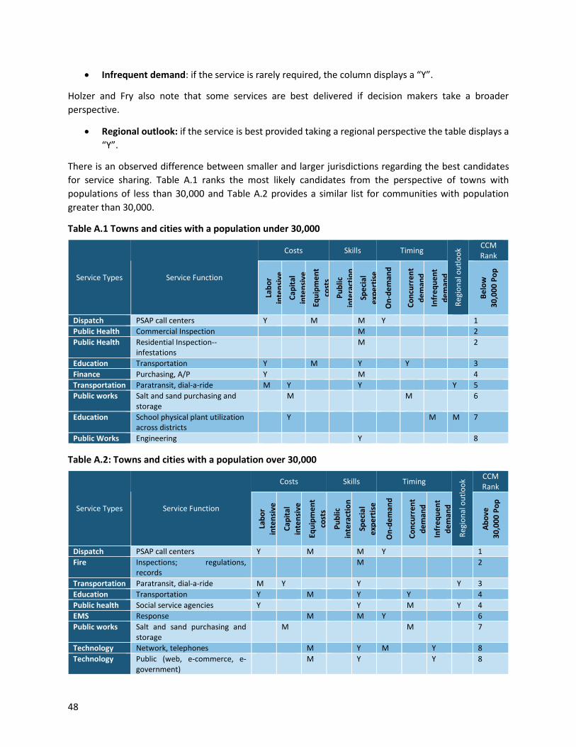
48

• Infrequent demand: if the service is rarely required, the column displays a “Y”.

Holzer and Fry also note that some services are best delivered if decision makers take a broader perspective.

• Regional outlook: if the service is best provided taking a regional perspective the table displays a “Y”.

There is an observed difference between smaller and larger jurisdictions regarding the best candidates for service sharing. Table A.1 ranks the most likely candidates from the perspective of towns with populations of less than 30,000 and Table A.2 provides a similar list for communities with population greater than 30,000.

Table A.1 Towns and cities with a population under 30,000

Service Types Service Function

Costs Skills Timing

Regi

onal

out

look

CCM Rank

Labo

r in

tens

ive

Capi

tal

inte

nsiv

e Eq

uipm

ent

cost

s Pu

blic

in

tera

ctio

n Sp

ecia

l ex

pert

ise

On-

dem

and

Conc

urre

nt

dem

and

Infr

eque

nt

dem

and

Belo

w

30,0

00 P

op

Dispatch PSAP call centers Y M M Y 1 Public Health Commercial Inspection M 2 Public Health Residential Inspection--

infestations M 2

Education Transportation Y M Y Y 3 Finance Purchasing, A/P Y M 4 Transportation Paratransit, dial-a-ride M Y Y Y 5 Public works Salt and sand purchasing and

storage M M 6

Education School physical plant utilization across districts

Y M M 7

Public Works Engineering Y 8 Table A.2: Towns and cities with a population over 30,000

Service Types Service Function

Costs Skills Timing

Regi

onal

out

look

CCM Rank

Labo

r in

tens

ive

Capi

tal

inte

nsiv

e

Equi

pmen

t co

sts

Publ

ic

inte

ract

ion

Spec

ial

expe

rtis

e

On-

dem

and

Conc

urre

nt

dem

and

Infr

eque

nt

dem

and

Abov

e 30

,000

Pop

Dispatch PSAP call centers Y M M Y 1 Fire Inspections; regulations,

records M 2

Transportation Paratransit, dial-a-ride M Y Y Y 3 Education Transportation Y M Y Y 4 Public health Social service agencies Y Y M Y 4 EMS Response M M Y 6 Public works Salt and sand purchasing and

storage M M 7

Technology Network, telephones M Y M Y 8 Technology Public (web, e-commerce, e-

government) M Y Y 8

49

It should be noted that there are overlaps and similarities in the two lists. For both groups, PSAP (911) call centers are the prime candidate for increased service sharing. But the approach to sharing should be on a regional or COG basis and should be adapted to the needs of the region. Other overlaps between the two lists include education transportation, paratransit (dial-a-ride), and salt/sand purchasing and storage.

The recommendation is that communities consider their delivery of these services carefully and engage with other potential partners in the assessment process outlined above.

4.0 CONCLUSIONS As demonstrated in a separate appendix, Connecticut local governments as a group are comparatively inexpensive by national standards. There are also numerous examples of service sharing involving Connecticut towns and cities. Nonetheless, CCM members recognize that greater efficiencies are achievable through service sharing.

This appendix has outlined a framework for thinking about service sharing and a process to that will help communities explore and engage in greater levels of shared services. In addition, specific opportunities have been identified for further exploration.

50

APPENDIX B: STATE ECONOMIC CONDITIONS

1. INTRODUCTION Connecticut faces a diverse set of demographic and economic headwinds. Population growth is slowing, annual increases in Gross Domestic Product are lagging, and employment growth is below national trends in key employment groups. Connecticut citizens and firms also face high state taxes and high-energy costs. None of these trends suggest a vibrant economic future. There are also some positive aspects of the state’s economy: Connecticut has a highly educated work force and among the highest per capita Gross Domestic Products among the 50 states.

This appendix provides a brief overview of the trends that face Connecticut. The intent of the review is to inform decisions-makers and prevent them from embracing incorrect assumptions about the status of the state’s economic future.

2. NATIONAL ECONOMIC TRENDS: COINCIDENT INDICATORS The review of the Connecticut economy begins by comparing trends in the Connecticut economy to trends in the United States and selected states. The initial comparison employs the Coincident Indicator (CI). The CI is generated by the Philadelphia Federal Reserve Bank and provides a standard economic index for each of the 50 states and the National economy. CI’s are reported monthly. The factors that are used to construct each state’s index are

• Nonagricultural Payroll Employment, • Employment Rate, • Average Hours Worked in Manufacturing, and • Real Wage and Salary Disbursements.

Figure B.1 reports the index (Year 2000 = 1) of the CI for the United States, Connecticut and New York. The reported period covers 2000-2016. The index of the CI illustrates a state’s relative trends. For example, the effect of the two national recessions that occurred during the period 2000-16 is clear for each state in figure B.1.

The first downturn is reflected in the dip in the index during the early part of the 2000-9 decade. As shown in figure B.1, the effect of the first downturn occurs earlier in Connecticut than it does in the U.S. economy. It is also a more acute response in Connecticut and it lasted for a longer period before an upturn occurs. The reaction of the Connecticut economy during the Great Recession is similar to the response during the first downturn but even more pronounced. New York on the other hand faired worse during the first recession, but has recovered more quickly than Connecticut since the Great Recession. Both Connecticut and New York lag behind broader national trends.

A significant takeaway from figure B.1 is that national business cycles, positive or negative, influence economic conditions in all states. Some states may experience more immediate, deeper, and longer lasting setbacks during downturns while others may grow more quickly during economic recoveries or expansion but no state is immune to the ups and downs of the national economy.

51

Understanding and, even more critical, appreciating the importance of the performance of the national economy tempers notions that a single state or a local government can dramatically alter or reverse national economic trends. The business cycle is not a respecter of states or regions.

Figure B.1: Coincident indicator of economic performance: 2000-2016

3. GROWTH IN GROSS DOMESTIC PRODUCT State Gross Domestic Product (GDP) is a comprehensive measure of the value of the goods and services produced annually in a state. A growing GDP reflects positive opportunities for both new and established firms. A slowing in the rate of growth in GDP suggests that a state faces challenges in creating and maintaining economic opportunities.

Table B.1 reports the annual compound rate of growth for selected periods of time for GDP for the U.S., Connecticut, and the states selected for comparison. The reported rates of growth confirm that the U.S. economy suffered during the period 2004-09. The compound rate of growth declined for the U.S. and every state during this period. The period 2010-15 shows a period of recovery for the selected states.

52

But the recovery has been uneven. Since the Great Recession, Connecticut’s economy, measured by GDP, did increase but had the slowest rate of change of all the states reported in table B.1. Connecticut has not had a robust recovery in GDP after the Great Recession. The last column in table B.1 is an index of rate of growth of the U.S. and selected states all indexed to Connecticut and confirms the slow growth rate in GDP during the recent recovery compared to the nation as a whole.

Table B.1: Annual Rate of Growth in State GDP for Selected Periods; U.S., Connecticut, and Selected States

State

Period Annual Rate of Change 2010-15

Indexed to Connecticut

2000-04 2005-9 2010-15 2000-15

United States 4.5 2.4 3.7 3.8 1.61 Connecticut 4.5 2.1 2.3 3.0 1.00 Massachusetts 3.3 2.7 3.6 3.4 1.57 New Jersey 4.1 2.1 2.9 3.1 1.26 New York 3.7 2.8 3.6 3.8 1.57 Florida 6.8 -1.2 3.9 4.0 1.70 Georgia 3.7 1.7 4.0 3.3 1.74 Maryland 6.4 3.5 3.0 4.3 1.30 North Carolina 4.7 3.4 3.7 4.0 1.61 Illinois 3.3 2.1 3.5 3.1 1.52 Michigan 2.2 -1.9 3.8 1.9 1.61 Ohio 3.6 0.5 4.2 3.0 1.83

Source: Bureau of Economic Analysis

The slow rate of increase since the end of the Great Recession is noteworthy when considered in relation to past periods. Between 2000-4 Connecticut’s growth in GDP was equal to the national average and exceeded some states. However, during the period following the Great Recession Connecticut’s rate of increase in GDP lags every state in the comparison group.

4. CONNECTICUT PERSONAL INCOME AND TOTAL TAXABLE RESOURCES Slow growth in GDP suggests Connecticut would have, at best, a modest level of personal income or wealth. This is currently not the situation in Connecticut. It has historically had a level of per capita personal income that is substantially above the average in the United States and that relatively high level of per capita income remains.

The U.S. Bureau of Economic Analysis (BEA) reports Connecticut had the highest per capita personal income among the states reported in figure B.2. The ranking of per capita personal income is shown in descending order (figure B.2.) Connecticut’s per capita personal income was significantly higher than the

53

next two highest states and remains in first place if all 50 states were included in the analysis. (Mississippi is included in figure B.2 and serves as an anchor, or the state with the lowest per capita income.)

Figure B.2: Per Capita Income and Per Capita Total Taxable Resources: Selected States

Source: U.S. Bureau of Economic Analysis and U.S. Treasury Department

Figure B.2 also reports a second measure of the wealth of a state, Total Taxable Resources (TTR). TTR is estimated annually for each state by the U.S. Treasury Department. TTR is intended to give a more complete picture of the ability of a state to fund state public services. Estimating TTR begins with state gross product (GDP) and then excludes items that would not be taxable under accepted broad definitions of income and adds in items that would be part of a broad definition of income. The results for TTR suggest that per capita income and TTR follow similar but not identical trends. However, the inclusion of TTR confirms that Connecticut currently leads the U.S. in terms of income and economic resources per person.

5. EDUCATIONAL ATTAINMENT The fact that personal per capita income and TTR in Connecticut are currently the highest among the 50 states may in part be explained by the concentration of college graduates in Connecticut. Among the 50 states Connecticut has one of the highest percentages of residents over 25 years of age with bachelor degrees and an equally notable percent of the population with graduate degrees. The relative significance of Connecticut’s higher education advantage is illustrated in figure B.3. With the exception of

$-

$10,000

$20,000

$30,000

$40,000

$50,000

$60,000

$70,000

$80,000

$90,000

$100,000

Per C

apita

l Dol

lars

Personal Income Total Taxable Resources

54

Massachusetts and Maryland, Connecticut’s education position exceeds that of every state in the comparison group for both the percentage of citizens with bachelor and graduate degrees. While education does not guarantee a higher income it contributes to earning power and eventually income levels.

Figure B.3: Percent of State Population over 25 with Bachelor’s Degree and Graduate Degree by statea

a. Numbers above bars indicate national rank Source: U.S. Census Bureau, American Community Survey

6. CONNECTICUT SALARIES The relative salaries for three employment groups, financial services, software development, and production, are reported because of their importance in the Connecticut, the U.S. and global economies.

Figure B.4 shows the relative levels of compensation after indexing the salaries of the selected employment groups from each state to Connecticut’s compensation levels. The results show that production workers in Connecticut receive the highest level of pay for production employment compared to the selected states. Connecticut’s production salaries exceed the compensation in some of the selected states by as much as one-third.

Many factors play into the compensation of a particular group within a state. A reason for the difference in compensation may be related to the relative complexity of the manufacturing occurring in Connecticut.

2 2

7 7 1116 17 19 21

2533 34

38 401

7

34

2

1114

5

10

29 3017

2231

0%

5%

10%

15%

20%

25%

Perc

ent o

f Pop

ulat

ion

25 a

nd o

ver

Bachelor's degree Graduate or professional degree

55

Connecticut has had a history of defense related production that may have led to an overall increase in compensation for production workers. Production workers in Connecticut are clearly doing better than similar workers in neighboring states, Mid-western states, and Coastal states.

Compensation for the financial sector does not show as much disparity between the states. Two states have compensation levels that are higher than those in Connecticut and four states are relatively close to Connecticut’s compensation levels. In five states the compensation for Software Developers exceeds the compensation level in Connecticut. In the states that fall below Connecticut the compensation levels that are reported are close to Connecticut’s.

Figure B.4: Salaries in Selected States for Production, Finance, and Software Compared to Connecticut

A more nuanced view of the rate of employment changes in the major industrial groups is given in table B.3. The table reports the percentage change in employment for five major employment groups over the five-year period 2011 (June) to 2015 (June).

Since 2011 some states have seen a modest rebound in manufacturing employment. Connecticut is not one of the states. The rate of growth in manufacturing in Connecticut is slower than every other state except for Maryland. The rate of growth in employment in finance, an area where it would be expected that Connecticut would have some advantage, is slower by a substantial amount than every other state except Virginia.

0

0.2

0.4

0.6

0.8

1

1.2

CONN MASS OH ILL FLA MICH NJ MD GA NY NC

INDE

X; C

ON

NEC

TICU

T =

1

STATE

PROD FIN SOFTWARE

56

Connecticut has experienced positive employment growth in four of the five industrial groupings but the rate of change again lags the other states with few exceptions.

Table B.3: Percent Change in Employment 2011 to 2015 by Industry Group

STATE INDUSTRY EMPLOYMENT GROUP MFG TRADE FINANCE PROFESSIONAL EDUC/HEALTH

Connecticut -2.64 4.51 0.29 7.06 3.81 NEIGHBORING STATES

Massachusetts -0.71 3.91 3.76 11.47 9.20 New Jersey 0.12 6.40 2.84 5.21 7.79 New York -1.52 4.35 3.59 9.24 10.78

COASTAL STATES Florida 11.45 11.85 10.72 18.01 12.05 Georgia 8.75 10.79 6.60 19.17 11.59 Maryland -2.91 4.62 2.52 7.87 7.87 North Carolina 4.79 10.10 7.27 15.54 5.99

INDUSTRIAL MID-WESTERN STATES Illinois -0.14 4.81 1.79 9.11 4.48 Michigan 13.41 6.30 10.31 13.39 5.46 Ohio 7.77 5.19 6.60 6.88 6.25

Source: Bureau of Labor Statistics

7. BUSINESS CLIMATE States are routinely ranked with respect to their business climate. Various business-focused magazines, policy organizations and the mainstream media do these rankings. Table B.4 lists selected rankings for Connecticut, Massachusetts, Illinois, and Georgia. The rankings reported are from Forbes, CNBC, Wall Street Journal Chief Executive, and the Tax Foundation. It is obvious that the rankings give mixed messages on many of the same questions. The Wall Street Journal ranks Massachusetts second in terms of doing business but Chief Executive ranks it at 45th. However, one conclusion that can be gained from the reported rankings is that Connecticut is viewed as a state with high taxes and high costs of doing business.

57

Table B.4: Selected State Business Climate Rankings

Source Dimension State Connecticut Massachusetts Illinois Georgia

Forbes

Quality of Life 4 3 14 32 Labor Supply 25 5 34 13

Economic Climate 44 8 29 21

Business Costs 45 50 29 23

CNBC

Cost of Doing Business 47 46 24 31

Infrastructure 47 42 16 4 Education 18 1 4 33

Wall Street Journal

Best and Worst for Doing Business 20 2 37 25

Chief Executive Business Climate 46 45 48 8

Tax Foundation

Overall Taxes 43 27 23 36 Personal Income Tax 37 13 16 42 Property Tax 49 45 46 21 Corporate Tax 49 45 46 21 Sales tax 43 27 23 36

Source: see column 1

8. CONCLUSIONS The State of Connecticut is facing a variety of challenges. Citizens in Connecticut benefit from high per capita income, high per capita GDP, and high education levels. The state also faces difficult issues. The rate of population growth is among the slowest in the U.S. The workforce is aging and certain important industries are losing employment. Some of these industries, notably manufacturing, are declining across the entire U.S., but the decline in Connecticut is more pronounced.

The cost of doing business is relatively high in Connecticut. Salaries are among the highest in the U.S. in some industries. Energy costs are also among the highest in the U.S., the higher costs are most notable when compared to states in the Coastal region of the U.S. and the states in the Mid-west.

By any comparison, the tax levels in Connecticut are also high. This is true for all taxes but for some taxes like the property tax may be a serious deterrent to business firms. The personal income tax is also relatively high and likely factors into many business and individual location decisions.

On the plus side the quality of life that is reported in national studies places Connecticut in the upper range of states. The dilemma for policy makers is to maintain the quality of life but at the same time find ways to make the state more attractive for population growth and business growth and retention.

58

APPENDIX C: ESTIMATED DISTRIBUTION OF LOCAL SALES TAX REVENUE As indicated in section 7, a share of the proposed one percent local sales tax should be used to complete the funding of PILOT programs, including funding the state property PILOT at 77% (total incremental cost: $164.1 millions) and for colleges and hospitals (total incremental cost: $159.7 million). The balance of local sales tax revenue ($346 million) should be distributed on the basis of fiscal need.

If state aid or a statewide tax, such as the proposed new local sales tax, is to be distributed at least partially on the basis of fiscal need, it is essential that a fair standard for assessing relative need be developed. The demands placed on local governments vary with demography, geography, climate, history and other factors often beyond the control of local governments. Until such time as a better metric can be developed and tested, we propose that the balance of local sales tax revenue be distributed using the same formula currently employed in the LoCIP program.

LOCAL CAPITAL IMPROVEMENT PROGRAM (LOCIP) The Local Capital Improvement Program (LoCIP) distributes funds to municipalities to reimburse the cost of eligible local capital improvement projects such as road, bridge or public building construction activities.7 The intent of the program is to provide capital improvement assistance to communities in need. Each year, OPM provides a formula-based entitlement to each municipality's available LoCIP balance. These funds can accumulate from year to year.

The formula used to calculate the local entitlement is given in state law (GCS Section 7- 536(c)). The formula combines four indicators into a single weighted allocation factor. The four indicators are:

1. The ratio of the total number of miles of improved and unimproved highways in each town to the total number of miles of improved and unimproved highways in all towns in the state (weight = 30%)

2. The density of each town multiplied by the population of the town, then divided by the sum of a similar calculation for all towns. (weight = 25%)

3. The population of each town multiplied by the inverse of the adjusted equalized net grand list per capita (or in other words, population squared, divided by the adjusted equalized net grand list). The resulting values for all the towns are added together and the value for each town is divided by the sum (weight = 25%)

4. The ratio of the population of each town to the population of the state (weight = 20%).

The OPM website includes a listing of all certified municipal entitlements through 2016.8 The entitlements have totaled $30 million each year since 2007. The 2016 allocations vary from a high of $1.98 million in Hartford to a low of $17,774 in Franklin. As noted, the annual allocation can be accumulated over time. Towns must apply for the reimbursement and the projects must be approved by OPM.

Without adding funds to the LoCIP program, the same formula can be used to allocate the share of new local sales tax revenue not used to complete funding for PILOT programs. Using the LoCIP formula, and

7 http://www.ct.gov/opm/cwp/view.asp?a=2985&q=383108 8 http://www.ct.gov/opm/lib/opm/igp/grants/locip/2007thru2016entitlementamountsweb.pdf

59

when combined with supplements to the PILOT programs as described in section 7, the estimated allocation of local sales tax revenue to each town will be as shown in table C.1.

Table C.1: Allocation of local sales tax based on additional PILOT reimbursements and LoCIP formula

Municipality

Additional PILOT funding

Remaining Sales Tax allocation

(LoCIP Formula,

$000)

Total Estimated Allocation

($000)

2014 General

Fund Revenue

($000)

Allocation as a percent of 2014 Gen.

Fund revenue (%)

State properties

($000)

College & Hospitals

($000)

Andover 47.5 - 325.3 372.8 Ansonia 277.0 - 2,038.2 2,315.2 64,113.6 3.6% Ashford 14.4 - 568.5 582.9 13,982.1 4.2% Avon 209.5 - 1,256.7 1,466.2 78,487.9 1.9% Barkhamsted 49.5 - 411.5 461.0 11,015.2 4.2% Beacon Falls 113.8 - 432.4 546.1 20,682.6 2.6% Berlin 61.1 - 1,450.6 1,511.7 74,527.8 2.0% Bethany 87.2 22.0 539.7 649.0 21,933.4 3.0% Bethel 84.1 22.6 1,370.1 1,476.8 69,635.6 2.1% Bethlehem 2.9 - 396.2 399.1 10,389.4 3.8% Bloomfield 301.2 278.2 1,458.1 2,037.4 81,498.8 2.5% Bolton 108.7 - 434.5 543.2 Bozrah 11.7 - 306.4 318.1 7,782.1 4.1% Branford 136.4 18.9 1,782.4 1,937.8 99,024.2 2.0% Bridgeport 5,976.5 10,877.5 27,862.3 44,716.3 519,814.1 8.6% Bridgewater 3.4 - 273.0 276.4 7,285.1 3.8% Bristol 223.1 814.8 5,440.7 6,478.6 187,210.4 3.5% Brookfield 71.3 - 1,198.1 1,269.4 76,772.6 1.7% Brooklyn 92.6 - 835.5 928.0 23,263.1 4.0% Burlington 134.6 - 854.2 988.7 Canaan 249.3 2.9 223.8 476.0 4,413.3 10.8% Canterbury 24.6 - 639.8 664.4 14,901.6 4.5% Canton 71.4 - 791.4 862.8 35,647.3 2.4% Chaplin 155.5 - 313.4 469.0 7,991.2 5.9% Cheshire 1,503.1 177.1 2,088.0 3,768.2 101,026.2 3.7% Chester 34.7 - 329.8 364.5 12,535.3 2.9% Clinton 84.9 - 974.9 1,059.8 47,378.4 2.2% Colchester 69.8 - 1,348.6 1,418.4 52,738.9 2.7% Colebrook 18.3 - 288.2 306.5 5,923.0 5.2% Columbia 17.8 - 456.0 473.8 16,520.1 2.9% Cornwall 45.0 - 376.5 421.4 6,241.8 6.8% Coventry 120.4 - 1,176.2 1,296.6 38,961.5 3.3% Cromwell 46.2 79.0 958.5 1,083.7 45,437.5 2.4% Danbury 5,613.9 1,836.4 6,434.6 13,884.9 225,626.5 6.2% Darien 247.6 - 1,283.4 1,531.0 125,841.9 1.2% Deep River 25.9 - 350.5 376.4

60

Municipality

Additional PILOT funding

Remaining Sales Tax allocation

(LoCIP Formula,

$000)

Total Estimated Allocation

($000)

2014 General

Fund Revenue

($000)

Allocation as a percent of 2014 Gen.

Fund revenue (%)

State properties

($000)

College & Hospitals

($000)

Derby 106.3 1,222.5 1,223.6 2,552.3 40,178.9 6.4% Durham 46.3 - 603.9 650.2 29,808.7 2.2% Eastford 15.7 - 263.9 279.6 5,244.0 5.3% East Granby 66.9 - 398.5 465.4 20,138.7 2.3% East Haddam 110.7 - 1,019.6 1,130.3 29,585.5 3.8% East Hampton

274.5 - 1,030.9 1,305.4 39,960.4 3.3%

East Hartford 1,837.2 710.8 5,176.9 7,724.9 172,482.0 4.5% East Haven 873.1 - 2,476.5 3,349.6 86,619.4 3.9% East Lyme 1,589.0 58.6 1,371.5 3,019.2 63,526.0 4.8% Easton 148.3 - 767.7 916.1 42,214.5 2.2% East Windsor 276.2 - 903.0 1,179.2 Ellington 18.5 - 1,216.7 1,235.2 49,485.7 2.5% Enfield 1,122.3 37.0 3,697.0 4,856.3 132,839.7 3.7% Essex 25.6 20.6 462.2 508.4 22,901.8 2.2% Fairfield 82.2 3,608.3 4,275.2 7,965.7 280,988.5 2.8% Farmington 7,889.7 43.3 1,580.4 9,513.4 92,615.7 10.3% Franklin 40.1 - 204.4 244.5 6,221.3 3.9% Glastonbury 116.3 2.4 2,350.6 2,469.3 149,925.7 1.6% Goshen 43.7 - 492.8 536.5 10,629.1 5.0% Granby 31.2 - 915.6 946.8 42,712.9 2.2% Greenwich 60.0 1,226.7 3,691.1 4,977.7 382,146.4 1.3% Griswold 155.7 - 1,060.4 1,216.0 32,285.2 3.8% Groton 2,608.4 54.9 2,446.0 5,109.3 Guilford 48.3 26.5 1,588.3 1,663.1 85,841.2 1.9% Haddam 161.8 - 852.6 1,014.4 29,173.8 3.5% Hamden 2,365.3 4,134.2 4,985.3 11,484.9 197,524.4 5.8% Hampton 75.5 - 323.6 399.1 6,069.9 6.6% Hartford 32,781.2 34,188.6 22,807.8 89,777.5 533,908.4 16.8% Hartland 246.6 - 220.0 466.5 7,134.3 6.5% Harwinton 13.1 - 576.1 589.2 Hebron 36.2 - 807.2 843.4 35,554.8 2.4% Kent 149.3 - 483.9 633.2 10,765.0 5.9% Killingly 629.1 - 1,658.4 2,287.4 52,656.9 4.3% Killingworth 244.3 - 615.7 860.0 20,935.7 4.1% Lebanon 80.5 - 831.3 911.8 23,630.5 3.9% Ledyard 52.5 - 1,285.6 1,338.1 50,571.6 2.6% Lisbon 17.8 - 327.3 345.0 13,695.0 2.5% Litchfield 181.1 - 945.6 1,126.7 28,187.8 4.0% Lyme 37.7 0.3 297.4 335.3 13,907.3 2.4%

61

Municipality

Additional PILOT funding

Remaining Sales Tax allocation

(LoCIP Formula,

$000)

Total Estimated Allocation

($000)

2014 General

Fund Revenue

($000)

Allocation as a percent of 2014 Gen.

Fund revenue (%)

State properties

($000)

College & Hospitals

($000)

Madison 1,180.3 - 1,274.8 2,455.1 75,349.3 3.3% Manchester 1,965.7 1,183.3 4,878.9 8,028.0 173,009.9 4.6% Mansfield 17,840.6 - 2,134.5 19,975.2 47,309.0 42.2% Marlborough 35.5 - 581.1 616.6 21,607.3 2.9% Meriden 1,006.7 1,715.8 5,880.6 8,603.2 181,695.2 4.7% Middlebury 27.5 - 638.8 666.3 29,923.9 2.2% Middlefield 24.3 - 365.9 390.2 17,060.1 2.3% Middletown 2,334.4 5,583.3 3,619.2 11,537.0 139,667.8 8.3% Milford 1,292.1 612.6 4,051.5 5,956.2 190,768.8 3.1% Monroe 27.9 - 1,553.9 1,581.8 78,820.8 2.0% Montville 592.2 - 1,681.1 2,273.3 56,735.1 4.0% Morris 34.2 - 250.5 284.7 8,495.6 3.4% Naugatuck 215.7 - 2,867.6 3,083.2 110,933.0 2.8% New Britain 8,252.2 3,678.4 11,442.5 23,373.0 219,495.6 10.6% New Canaan 116.9 - 1,335.6 1,452.5 New Fairfield 48.2 - 929.3 977.5 50,545.8 1.9% New Hartford 45.8 - 727.3 773.1 22,670.4 3.4% New Haven 14,017.9 57,074.6 19,028.9 90,121.4 495,516.8 18.2% Newington 1,740.1 423.0 2,412.6 4,575.7 105,456.4 4.3% New London 929.5 5,508.0 3,561.5 9,999.0 New Milford 76.5 316.9 2,216.6 2,610.0 Newtown 731.0 - 2,395.7 3,126.7 110,861.9 2.8% Norfolk 219.8 65.3 368.2 653.2 North Branford 13.2 3.3 1,025.9 1,042.5 47,780.2 2.2%

North Canaan 57.1 - 345.9 403.0

North Haven 280.7 884.6 1,786.1 2,951.5 87,545.8 3.4% North Stonington 55.3 - 553.2 608.4 20,002.2 3.0%

Norwalk 823.1 2,146.7 7,288.9 10,258.7 313,371.1 3.3% Norwich 1,597.3 1,107.1 3,703.1 6,407.5 115,652.3 5.5% Old Lyme 70.9 47.9 567.8 686.6 33,998.4 2.0% Old Saybrook 112.7 - 773.4 886.1 40,503.4 2.2% Orange 27.8 339.7 1,164.7 1,532.2 62,536.4 2.5% Oxford 592.8 - 1,100.8 1,693.6 Plainfield 135.0 56.4 1,495.1 1,686.5 44,096.6 3.8% Plainville 41.5 - 1,436.5 1,478.0 60,252.4 2.5% Plymouth 28.9 - 1,087.6 1,116.5 Pomfret 112.5 - 540.4 652.9 13,597.5 4.8%

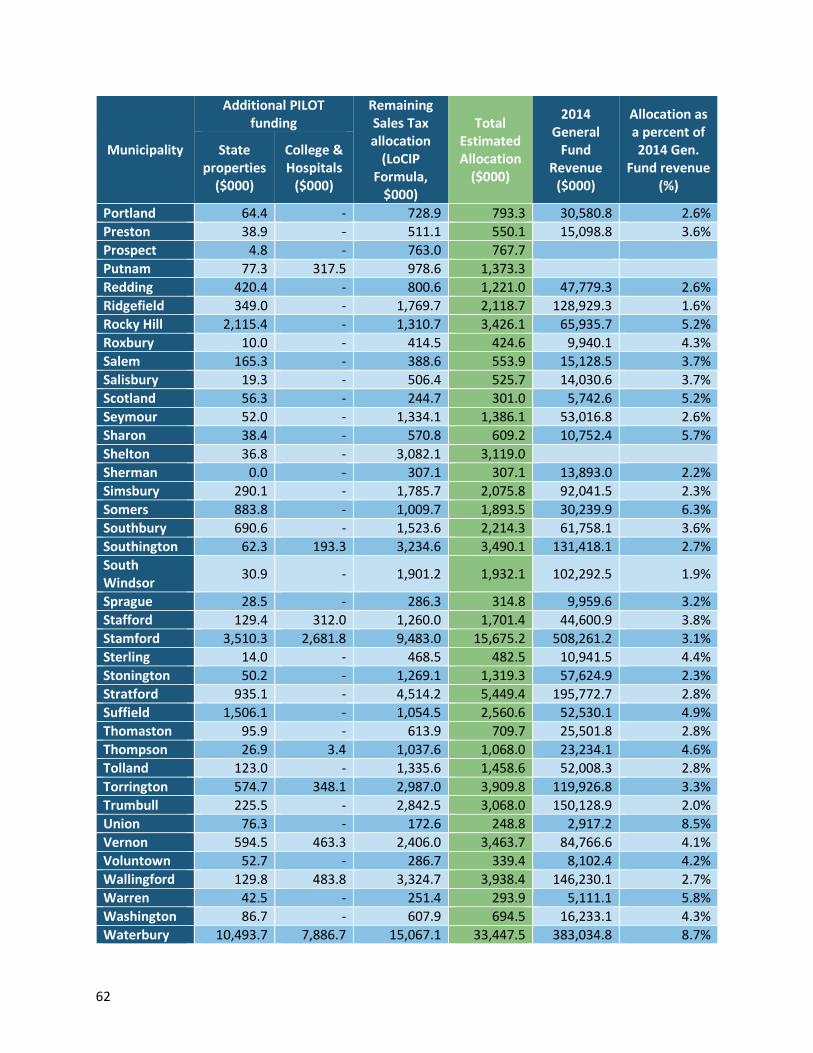
62

Municipality

Additional PILOT funding

Remaining Sales Tax allocation

(LoCIP Formula,

$000)

Total Estimated Allocation

($000)

2014 General

Fund Revenue

($000)

Allocation as a percent of 2014 Gen.

Fund revenue (%)

State properties

($000)

College & Hospitals

($000)

Portland 64.4 - 728.9 793.3 30,580.8 2.6% Preston 38.9 - 511.1 550.1 15,098.8 3.6% Prospect 4.8 - 763.0 767.7 Putnam 77.3 317.5 978.6 1,373.3 Redding 420.4 - 800.6 1,221.0 47,779.3 2.6% Ridgefield 349.0 - 1,769.7 2,118.7 128,929.3 1.6% Rocky Hill 2,115.4 - 1,310.7 3,426.1 65,935.7 5.2% Roxbury 10.0 - 414.5 424.6 9,940.1 4.3% Salem 165.3 - 388.6 553.9 15,128.5 3.7% Salisbury 19.3 - 506.4 525.7 14,030.6 3.7% Scotland 56.3 - 244.7 301.0 5,742.6 5.2% Seymour 52.0 - 1,334.1 1,386.1 53,016.8 2.6% Sharon 38.4 - 570.8 609.2 10,752.4 5.7% Shelton 36.8 - 3,082.1 3,119.0 Sherman 0.0 - 307.1 307.1 13,893.0 2.2% Simsbury 290.1 - 1,785.7 2,075.8 92,041.5 2.3% Somers 883.8 - 1,009.7 1,893.5 30,239.9 6.3% Southbury 690.6 - 1,523.6 2,214.3 61,758.1 3.6% Southington 62.3 193.3 3,234.6 3,490.1 131,418.1 2.7% South Windsor 30.9 - 1,901.2 1,932.1 102,292.5 1.9%

Sprague 28.5 - 286.3 314.8 9,959.6 3.2% Stafford 129.4 312.0 1,260.0 1,701.4 44,600.9 3.8% Stamford 3,510.3 2,681.8 9,483.0 15,675.2 508,261.2 3.1% Sterling 14.0 - 468.5 482.5 10,941.5 4.4% Stonington 50.2 - 1,269.1 1,319.3 57,624.9 2.3% Stratford 935.1 - 4,514.2 5,449.4 195,772.7 2.8% Suffield 1,506.1 - 1,054.5 2,560.6 52,530.1 4.9% Thomaston 95.9 - 613.9 709.7 25,501.8 2.8% Thompson 26.9 3.4 1,037.6 1,068.0 23,234.1 4.6% Tolland 123.0 - 1,335.6 1,458.6 52,008.3 2.8% Torrington 574.7 348.1 2,987.0 3,909.8 119,926.8 3.3% Trumbull 225.5 - 2,842.5 3,068.0 150,128.9 2.0% Union 76.3 - 172.6 248.8 2,917.2 8.5% Vernon 594.5 463.3 2,406.0 3,463.7 84,766.6 4.1% Voluntown 52.7 - 286.7 339.4 8,102.4 4.2% Wallingford 129.8 483.8 3,324.7 3,938.4 146,230.1 2.7% Warren 42.5 - 251.4 293.9 5,111.1 5.8% Washington 86.7 - 607.9 694.5 16,233.1 4.3% Waterbury 10,493.7 7,886.7 15,067.1 33,447.5 383,034.8 8.7%

63

Municipality

Additional PILOT funding

Remaining Sales Tax allocation

(LoCIP Formula,

$000)

Total Estimated Allocation

($000)

2014 General

Fund Revenue

($000)

Allocation as a percent of 2014 Gen.

Fund revenue (%)

State properties

($000)

College & Hospitals

($000)

Waterford 665.7 85.0 1,368.5 2,119.2 82,162.3 2.6% Watertown 98.3 - 1,801.3 1,899.6 66,133.8 2.9% Westbrook 70.0 25.8 494.2 590.0 26,492.3 2.2% West Hartford 701.7 1,481.5 5,040.2 7,223.4 243,521.9 3.0%

West Haven 140.1 3,074.1 6,688.3 9,902.6 151,006.8 6.6% Weston 15.2 - 752.6 767.9 67,933.6 1.1% Westport 1,952.6 251.6 1,685.1 3,889.3 195,114.3 2.0% Wethersfield 571.0 12.5 2,111.1 2,694.6 90,082.6 3.0% Willington 103.8 - 691.9 795.7 16,325.2 4.9% Wilton 314.4 - 1,301.5 1,615.9 117,358.4 1.4% Winchester 187.2 58.9 1,027.4 1,273.4 Windham 6,831.6 912.9 3,045.9 10,790.5 Windsor 126.7 - 2,088.2 2,214.9 101,114.3 2.2% Windsor Locks 244.9 - 921.5 1,166.4 46,740.5 2.5%

Wolcott 4.9 - 1,306.9 1,311.8 50,475.9 2.6% Woodbridge 40.9 0.1 744.2 785.2 45,208.8 1.7% Woodbury 1.5 - 902.7 904.2 31,282.9 2.9% Woodstock 23.7 - 960.8 984.4 21,424.5 4.6% Other local entities 168.7 880.1 1,048.9

Total 164,062.1 159,683.5 345,934.2 669,679.8 5.20a a. Weighted average of available towns

Source: Calculations by the author

64

APPENDIX D: SUPPLEMENTAL INFORMATION ON THE SIZE AND FISCAL

STRUCTURE OF GOVERNMENT IN CONNECTICUT An informed discussion of revenue needs and service efficiency in Connecticut requires an accurate understanding of the relative size of state and local government in the state. The purpose of this appendix is to provide that context largely in comparison with other states.

1. CROSS-STATE COMPARISONS Table D.1 reports total state and local taxes per capita and total taxes as a percent of Total Taxable Resources (TTR) for 2014, along with comparisons to the national average and national ranks.

Table D.1: Connecticut total state and local taxes compared to other states: 2014

State Per capita ($)

National Rank

Percent of U.S. Average

Percent of Total Taxable Resources

National Rank

Percent of U.S. average

U.S. Average 4,680 6.94% Connecticut 7,255 5 155% 7.85% 8 113% Massachusetts 6,018 7 129% 6.66% 31 96% New Jersey 6,458 6 138% 7.51% 14 108% New York 8,423 3 180% 9.30% 6 134% Rhode Island 5,172 15 111% 7.47% 17 108% Florida 3,325 47 71% 5.98% 42 86% Illinois 5,504 13 118% 7.65% 12 110% Maryland 5,609 11 120% 6.96% 26 100% Michigan 3,774 35 81% 6.55% 33 94% North Carolina 3,625 39 77% 6.29% 36 91% Ohio 4,208 27 90% 6.68% 30 96% Pennsylvania 4,708 18 101% 7.02% 23 101% Alabama 3,004 51 64% 5.95% 43 86% Alaska 7,559 4 162% 8.98% 7 129% Arizona 3,350 46 72% 7.15% 21 103% Arkansas 3,756 36 80% 7.43% 18 107% California 5,464 14 117% 7.61% 13 110% Colorado 4,370 24 93% 5.91% 44 85% Delaware 4,412 22 94% 5.54% 49 80% District of Columbia 9,679 2 207% 9.49% 3 137%

Georgia 3,380 45 72% 5.53% 50 80% Hawaii 5,721 9 122% 10.10% 2 146% Idaho 3,237 48 69% 6.81% 28 98% Indiana 3,749 37 80% 6.09% 38 88% Iowa 4,426 21 95% 6.71% 29 97% Kansas 4,382 23 94% 6.98% 25 101% Kentucky 3,607 40 77% 6.85% 27 99% Louisiana 3,890 32 83% 6.08% 39 88% Maine 4,805 17 103% 9.39% 5 135% Minnesota 5,645 10 121% 7.49% 16 108% Mississippi 3,503 43 75% 7.77% 10 112% Missouri 3,475 44 74% 5.78% 45 83% Montana 3,841 34 82% 7.51% 15 108% Nebraska 4,883 16 104% 6.99% 24 101% Nevada 3,882 33 83% 7.12% 22 103%

65

State Per capita ($)

National Rank

Percent of U.S. Average

Percent of Total Taxable Resources

National Rank

Percent of U.S. average

New Hampshire 4,325 25 92% 6.02% 40 87% New Mexico 3,972 30 85% 7.66% 11 110% North Dakota 9,747 1 208% 10.91% 1 157% Oklahoma 3,567 41 76% 6.00% 41 86% Oregon 4,103 28 88% 6.65% 32 96% South Carolina 3,221 49 69% 6.53% 34 94% South Dakota 3,687 38 79% 5.68% 47 82% Tennessee 3,093 50 66% 5.57% 48 80% Texas 4,050 29 87% 5.70% 46 82% Utah 3,506 42 75% 6.26% 37 90% Vermont 5,540 12 118% 9.41% 4 136% Virginia 4,209 26 90% 5.51% 51 79% Washington 4,563 20 98% 6.37% 35 92% West Virginia 3,957 31 85% 7.82% 9 113% Wisconsin 4,584 19 98% 7.16% 20 103% Wyoming 5,950 8 127% 7.16% 19 103%

Source: U.S. Census, State and Local Finance, 2014 data

Table D.2 reports on property taxes per capita and as a percentage of TTR, again with a comparison to the national average and national rankings for each state.

Table D.2: Connecticut Property taxes compared to other states: 2014

State Per capita ($)

National Rank

Percent of U.S. Average

Percent of Total Taxable Resources

National Rank

Percent of U.S. average

U.S. Average 1,464 2.17% Connecticut 2,776 4 190% 3.00% 8 138% Massachusetts 2,183 9 149% 2.41% 15 111% New Jersey 3,069 2 210% 3.57% 4 164% New York 2,585 6 177% 2.85% 10 131% Rhode Island 2,308 8 158% 3.33% 5 154% Florida 1,185 30 81% 2.13% 22 98% Illinois 2,009 11 137% 2.79% 11 129% Maryland 1,493 17 102% 1.85% 33 85% Michigan 1,335 27 91% 2.32% 16 107% North Carolina 952 40 65% 1.65% 40 76% Ohio 1,204 29 82% 1.91% 29 88% Pennsylvania 1,405 22 96% 2.09% 24 96% Alabama 522 51 36% 1.04% 51 48% Alaska 2,641 5 180% 3.14% 6 145% Arizona 987 34 67% 2.11% 23 97% Arkansas 674 49 46% 1.33% 46 61% California 1,389 23 95% 1.93% 28 89% Colorado 1,367 24 93% 1.85% 34 85% Delaware 829 46 57% 1.04% 50 48% District of Columbia 3,143 1 215% 3.08% 7 142%

Georgia 1,089 32 74% 1.78% 35 82% Hawaii 983 35 67% 1.74% 37 80% Idaho 928 41 63% 1.95% 27 90% Indiana 971 36 66% 1.58% 42 73% Iowa 1,526 16 104% 2.31% 17 107% Kansas 1,437 20 98% 2.29% 19 105% Kentucky 737 47 50% 1.40% 45 64%

66

State Per capita ($)

National Rank

Percent of U.S. Average

Percent of Total Taxable Resources

National Rank

Percent of U.S. average

Louisiana 839 44 57% 1.31% 47 60% Maine 1,918 12 131% 3.75% 3 173% Minnesota 1,412 21 96% 1.87% 32 86% Mississippi 917 42 63% 2.03% 25 94% Missouri 961 38 66% 1.60% 41 74% Montana 1,466 18 100% 2.87% 9 132% Nebraska 1,759 13 120% 2.52% 14 116% Nevada 954 39 65% 1.75% 36 81% New Hampshire 2,859 3 195% 3.98% 1 183% New Mexico 732 48 50% 1.41% 44 65% North Dakota 1,121 31 77% 1.26% 48 58% Oklahoma 624 50 43% 1.05% 49 48% Oregon 1,351 26 92% 2.19% 21 101% South Carolina 1,080 33 74% 2.19% 20 101% South Dakota 1,303 28 89% 2.01% 26 92% Tennessee 830 45 57% 1.49% 43 69% Texas 1,637 15 112% 2.31% 18 106% Utah 970 37 66% 1.73% 38 80% Vermont 2,338 7 160% 3.97% 2 183% Virginia 1,459 19 100% 1.91% 30 88% Washington 1,366 25 93% 1.91% 31 88% West Virginia 852 43 58% 1.69% 39 78% Wisconsin 1,657 14 113% 2.59% 12 119% Wyoming 2,111 10 144% 2.54% 13 117%

Source: U.S. Census, State and Local Finance, 2014 data

Table D.3 lists the median income and median property tax for each state and the resulting ratio of the two. The point of the table is to show how the median household in each state is impacted by the property tax. The national average median property tax on owner-occupied housing is just over 3 percent of median income for such households. However, the range is from 7.7 percent in New Jersey to less than one percent in Alabama.

Table D.3: Median income and median property tax by state

State Median income, owner-occupied

housing

Median real estate taxes

paid

Median tax as a percent of

median income

National Rank

Percent of national average

United States 71,027 2,149 3.03% Connecticut 95,111 5,327 5.60% 3 185.1% Massachusetts 95,027 3,989 4.20% 9 138.7% New Jersey 96,795 7,410 7.66% 1 253.0% New York 83,471 4,600 5.51% 4 182.1% Rhode Island 83,312 3,884 4.66% 7 154.1% Florida 59,864 1,686 2.82% 23 93.1% Illinois 75,854 3,995 5.27% 6 174.1% Maryland 96,105 3,142 3.27% 19 108.1% Michigan 62,140 2,174 3.50% 16 115.6% North Carolina 60,968 1,322 2.17% 30 71.7% Ohio 65,825 2,032 3.09% 20 102.0% Pennsylvania 69,281 2,533 3.66% 11 120.8%

67

State Median income, owner-occupied

housing

Median real estate taxes

paid

Median tax as a percent of

median income

National Rank

Percent of national average

Alabama 56,355 543 0.96% 51 31.8% Alaska 89,458 2,956 3.30% 18 109.2% Arizona 63,421 1,356 2.14% 32 70.7% Arkansas 52,734 693 1.31% 48 43.4% California 87,279 3,104 3.56% 14 117.5% Colorado 80,854 1,489 1.84% 38 60.9% Delaware 72,178 1,243 1.72% 42 56.9% District of Columbia 124,061 2,665 2.15% 31 71.0%

Georgia 65,864 1,397 2.12% 36 70.1% Hawaii 91,884 1,406 1.53% 46 50.6% Idaho 58,462 1,246 2.13% 34 70.4% Indiana 62,522 1,085 1.74% 41 57.4% Iowa 66,404 1,916 2.89% 21 95.4% Kansas 68,253 1,849 2.71% 25 89.5% Kentucky 56,731 1,042 1.84% 39 60.7% Louisiana 60,801 707 1.16% 50 38.4% Maine 62,263 2,259 3.63% 12 119.9% Minnesota 77,835 2,200 2.83% 22 93.4% Mississippi 50,644 813 1.61% 45 53.1% Missouri 63,076 1,387 2.20% 29 72.7% Montana 61,103 1,652 2.70% 26 89.4% Nebraska 70,440 2,467 3.50% 15 115.8% Nevada 69,324 1,481 2.14% 33 70.6% New Hampshire 86,182 5,100 5.92% 2 195.6% New Mexico 55,815 1,188 2.13% 35 70.3% North Dakota 77,404 1,722 2.22% 28 73.5% Oklahoma 60,256 1,036 1.72% 43 56.8% Oregon 70,006 2,563 3.66% 10 121.0% South Carolina 57,557 798 1.39% 47 45.8% South Dakota 67,114 1,879 2.80% 24 92.5% Tennessee 59,310 1,062 1.79% 40 59.2% Texas 71,728 2,578 3.59% 13 118.8% Utah 76,222 1,472 1.93% 37 63.8% Vermont 69,601 3,795 5.45% 5 180.2% Virginia 81,739 1,948 2.38% 27 78.8% Washington 80,718 2,805 3.48% 17 114.9% West Virginia 50,151 607 1.21% 49 40.0% Wisconsin 70,469 3,248 4.61% 8 152.3% Wyoming 72,458 1,196 1.65% 44 54.6%

Source: U.S. Census, American Community Survey

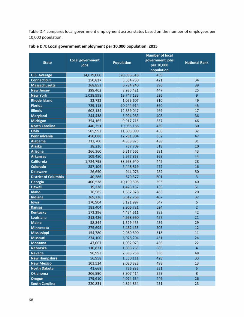
68

Table D.4 compares local government employment across states based on the number of employees per 10,000 population.

Table D.4: Local government employment per 10,000 population: 2015

State Local government jobs Population

Number of local government jobs

per 10,000 population

National Rank

U.S. Average 14,079,000 320,896,618 439 Connecticut 150,817 3,584,730 421 34 Massachusetts 268,853 6,784,240 396 39 New Jersey 399,463 8,935,421 447 25 New York 1,038,998 19,747,183 526 9 Rhode Island 32,732 1,055,607 310 49 Florida 729,115 20,244,914 360 45 Illinois 602,134 12,839,047 469 17 Maryland 244,438 5,994,983 408 36 Michigan 354,165 9,917,715 357 46 North Carolina 440,251 10,035,186 439 30 Ohio 505,992 11,605,090 436 32 Pennsylvania 450,088 12,791,904 352 47 Alabama 212,700 4,853,875 438 31 Alaska 38,216 737,709 518 10 Arizona 266,360 6,817,565 391 43 Arkansas 109,450 2,977,853 368 44 California 1,724,795 38,993,940 442 28 Colorado 257,106 5,448,819 472 16 Delaware 26,650 944,076 282 50 District of Columbia 40,286 670,377 601 3 Georgia 400,528 10,199,398 393 40 Hawaii 19,238 1,425,157 135 51 Idaho 76,585 1,652,828 463 20 Indiana 269,236 6,612,768 407 37 Iowa 170,904 3,121,997 547 6 Kansas 181,404 2,906,721 624 2 Kentucky 173,296 4,424,611 392 42 Louisiana 213,426 4,668,960 457 21 Maine 58,344 1,329,453 439 29 Minnesota 275,695 5,482,435 503 12 Mississippi 154,780 2,989,390 518 11 Missouri 274,100 6,076,204 451 24 Montana 47,067 1,032,073 456 22 Nebraska 110,821 1,893,765 585 4 Nevada 96,993 2,883,758 336 48 New Hampshire 56,958 1,330,111 428 33 New Mexico 103,524 2,080,328 498 13 North Dakota 41,668 756,835 551 5 Oklahoma 206,590 3,907,414 529 8 Oregon 179,610 4,024,634 446 26 South Carolina 220,831 4,894,834 451 23

69

State Local government jobs Population

Number of local government jobs

per 10,000 population

National Rank

South Dakota 46,443 857,919 541 7 Tennessee 277,007 6,595,056 420 35 Texas 1,279,943 27,429,639 467 18 Utah 120,902 2,990,632 404 38 Vermont 29,941 626,088 478 15 Virginia 372,700 8,367,587 445 27 Washington 332,913 7,160,290 465 19 West Virginia 72,197 1,841,053 392 41 Wisconsin 276,138 5,767,891 479 14 Wyoming 46,609 586,555 795 1

Source: U.S. Bureau of Economic Analysis and U.S. Census Bureau

Finally, table D.5 reports the level of total 2014 current expenditures for states and local governments as a percent of TTR. Local government expenditures are reported separately for non-education and the combined elementary and secondary education functions. Total current expenditures include education, libraries, public welfare, hospitals, health, employment security administration, veteran’s services, transportation, public safety, environment and housing (including parks and recreation), and governmental administration. Excluded are capital outlays, interest on general debt, miscellaneous commercial activities, and utilities.

Table D.5: Total 2014 Current Expenditures as a Percent of Total Taxable Resources by Level of Government

State

Percent of Total Taxable Resources National Rank

State Expendi-tures (%)

Local Non-Education Expendi-tures (%)

Local Elem. &

Sec. Expendi-tures (%)

Total State &

Local (%)

State Expendi-

tures

Local Non-Education Expendi-

tures

Local Elem. &

Sec. Expendi-

tures

Total State &

Local

U.S. Average 4.75 2.79 2.47 10.01 Connecticut 4.51 1.26 2.54 8.32 37 50 25 47 Massachusetts 4.80 1.31 2.26 8.37 31 48 42 44 New Jersey 4.15 1.70 2.91 8.77 41 42 13 43 New York 4.11 3.29 3.01 10.41 43 9 8 27 Rhode Island 6.27 1.66 2.99 10.92 14 43 9 19 Florida 4.14 3.62 2.20 9.96 42 6 43 33 Illinois 3.71 2.57 2.58 8.85 49 23 23 41 Maryland 4.68 2.20 2.37 9.25 34 31 32 40 Michigan 5.38 2.80 2.70 10.89 22 17 20 20 North Carolina 4.60 3.82 2.14 10.56 35 5 47 25 Ohio 5.29 2.82 2.73 10.84 23 16 18 23 Pennsylvania 5.23 2.47 2.86 10.56 24 27 14 26 Alabama 6.26 3.10 2.85 12.20 15 10 15 11 Alaska 8.68 2.94 2.93 14.54 4 11 12 3 Arizona 6.19 2.91 2.31 11.41 16 14 37 16 Arkansas 7.71 1.63 2.97 12.31 8 45 10 9 California 4.44 4.19 2.26 10.88 38 3 41 21 Colorado 3.79 2.59 1.99 8.36 46 21 49 45 Delaware 7.11 0.96 2.33 10.40 10 51 36 28

70

State

Percent of Total Taxable Resources National Rank

State Expendi-tures (%)

Local Non-Education Expendi-tures (%)

Local Elem. &

Sec. Expendi-tures (%)

Total State &

Local (%)

State Expendi-

tures

Local Non-Education Expendi-

tures

Local Elem. &

Sec. Expendi-

tures

Total State &

Local

District of Columbia 10.24 3.13 13.37 1 3 6

Georgia 3.92 2.35 2.56 8.83 45 30 24 42 Hawaii 10.05 2.01 12.05 1 36 13 Idaho 5.77 2.76 2.40 10.93 20 18 28 18 Indiana 4.94 2.42 2.15 9.51 29 28 46 37 Iowa 5.53 2.68 2.63 10.84 21 20 22 22 Kansas 5.11 2.55 2.54 10.20 25 26 26 30 Kentucky 7.56 1.50 2.36 11.42 9 46 34 15 Louisiana 5.87 2.76 2.40 11.03 18 19 29 17 Maine 8.42 1.90 3.27 13.59 5 40 2 5 Minnesota 5.10 2.56 2.36 10.02 26 24 35 32 Mississippi 7.78 4.04 3.02 14.83 7 4 7 2 Missouri 4.73 2.18 2.47 9.38 33 32 27 39 Montana 6.77 2.42 3.06 12.25 11 29 5 10 Nebraska 4.56 2.14 2.74 9.44 36 33 17 38 Nevada 3.75 3.41 2.39 9.55 47 8 30 36 New Hampshire 3.61 1.75 2.80 8.16 50 41 16 49

New Mexico 8.77 2.85 2.73 14.34 3 15 19 4 North Dakota 4.25 1.33 1.94 7.52 40 47 50 51 Oklahoma 5.85 1.97 2.27 10.09 19 37 40 31 Oregon 6.53 2.92 2.38 11.83 13 13 31 14 South Carolina 6.64 3.46 2.96 13.06 12 7 11 7 South Dakota 4.39 1.65 2.12 8.16 39 44 48 48 Tennessee 5.02 2.56 2.37 9.95 28 25 33 34 Texas 3.71 2.10 2.17 7.99 48 34 44 50 Utah 6.05 1.94 2.29 10.28 17 38 38 29 Vermont 9.73 1.26 4.07 15.07 2 49 1 1 Virginia 3.98 2.07 2.27 8.32 44 35 39 46 Washington 4.94 2.57 2.16 9.67 30 22 45 35 West Virginia 7.82 1.91 3.08 12.82 6 39 4 8 Wisconsin 5.08 2.93 2.67 10.67 27 12 21 24 Wyoming 4.79 4.36 3.04 12.19 32 2 6 12

Source: U.S. Census Bureau, State and Local Finance; U.S. Department of Treasury

2. PUBLIC TAX REVENUES The analysis of public tax revenue in table D.1 is based on per capita tax collections as reported by the U.S. Census Bureau. The following tables take a slightly different approach and compare state tax burdens by indexing the per capita amount from each state against Connecticut’s per capita amount. The indexed values cover three years, 2005, 2010, and 2013. The overall conclusion from the following tables is that state and local taxes in Connecticut are relatively high. At the same time, revenues from other sources are relatively low.

2.1 The Personal Income Tax Table D.6 reports on the personal income tax. In 2005, per capita collection of personal income taxes in the states of Maryland, Massachusetts and New York exceeded that of Connecticut. This same pattern is

71

found in 2010 and 2013. In all other states, the income taxes per capita were below Connecticut’s. A take away is that Connecticut relies heavily on the income tax. The next observation is that the relative importance of the personal income tax in the comparison states has declined over time relative to the tax in Connecticut.

Table D.6: Per Capita Personal Income Tax Revenue for Selected States Indexed to Connecticut

State Year 2005 2010 2013

Connecticut 1.00 1.00 1.00 Neighboring States

Massachusetts 1.05 0.96 0.88 New Jersey 0.77 0.73 0.63 New York

1.27 1.36 1.17

Coastal States Florida 0 0 0 Georgia 0.57 0.45 0.40 Maryland 1.14 1.06 0.95 North Carolina 0.67 0.59 0.52

Industrial Midwest States Illinois 0.44 0.46 0.59 Michigan 0.46 0.37 0.40 Ohio 0.80 0.66 0.58 Source: U.S. Census: State and Local Government Finance

2.2 The Sales Tax The sales tax in Connecticut has a pattern similar to the state personal income tax. Table D.7 shows that, with the exception of New York and Florida, the per capita sales tax is higher in Connecticut than every other state in the comparison group. Of course, Florida does not have a personal income tax and relies heavily on the sales tax. Like the personal income tax, Connecticut’s reliance on the sales tax has increased over the reported time periods when compared to the states in table D.7.

Table D.7: Per capita sales tax revenue for selected states, indexed to Connecticut

State Year 2005 2010 2013

Connecticut 1.00 1.00 1.00 Neighboring States

Massachusetts 0.64 0.84 0.62 New Jersey 0.81 0.87 0.74 New York 1.04 1.20 1.06

Coastal States Florida 1.14 1.06 0.94 Georgia 0.76 0.76 0.66 Maryland 0.69 0.79 0.73

72

State Year 2005 2010 2013

North Carolina 0.74 0.82 0.66 Industrial Midwest States

Illinois 0.90 0.88 0.78 Michigan 0.80 0.86 0.67 Ohio 0.76 0.82 0.73

Source: U.S. Census, State and Local Government Finance

2.3 The Corporate Income Tax The per capita corporate income taxes in the comparison states are by and large evenly split between being higher or lower than Connecticut’s (table D.8). The neighboring states of Massachusetts, New Jersey, and New York have corporate income taxes that on a per capita basis are often at least double those of Connecticut’s and in the case of New York approaching four times as high. Except for Maryland, the per capita corporate income tax in the Coastal states is much lower than Connecticut’s. And Connecticut, like most states, places little reliance on the corporate income tax.

Table D.8: Per capita corporate income tax for selected states indexed to Connecticut

State Year 2005 2010 2013

Connecticut 1.00 1.00 1.00 Neighboring States

Massachusetts 2.24 1.97 2.63 New Jersey 1.57 1.64 1.61 New York 2.23 3.29 3.71

Coastal States Florida 0.61 0.67 0.66 Georgia 0.49 0.50 0.50 Maryland 0.88 1.08 1.01 North Carolina 0.89 0.95 .82

Industrial Midwest States Illinois 1.06 1.47 2.18 Michigan 1.16 0.45 0.57 Ohio 0.72 0.15 0.27

Source: U.S. Census, State and Local Government Finance

2.4 The Property Tax As in most states, the property tax is a local government revenue source in Connecticut. Unlike most states, the property tax in Connecticut is essentially the only local government tax revenue. The results reported in table D.9 are once again similar to the results in tables D.7 and D.8. Connecticut’s per capita property tax is higher than the per capita property tax in every other state except for New Jersey. One difference from the other taxes is that the ratios between Connecticut property tax and the other states are relatively stable over the three time periods.

73

Table D.9: Per capita property revenue for selected states indexed to Connecticut

State Period 2005 2010 2013

Connecticut 1.00 1.00 1.00 Neighboring States

Massachusetts 0.79 0.76 0.76 New Jersey 1.O9 1.09 1.10 New York 0.87 0.90 0.91

Coastal States Florida 0.45 0.58 0.56 Georgia 0.45 0.42 0.37 Maryland 0.49 0.57 0.55 North Carolina 0.36 0.36 0.33

Industrial Midwest States Illinois 0.71 0.72 0.73 Michigan 0.63 0.56 0.48 Ohio 0.51 0.44 0.45 Source: U.S. Census, State and Local Government Finance

3. CONNECTICUT PROPERTY TAXES ARE HIGH There is no question that property taxes in Connecticut are high compared to other states. A common metric for assessing the relative size of the property tax is to compare property tax revenue to Gross Domestic Product (GDP). Total GDP measures the total value of goods and services produced in a state in all sectors, including government. To compare the private sector burden of the property tax, it is helpful to use only private sector GDP. Based on the most current data available (FY 2013), the total property tax collected in Connecticut represented over 4.5% of private sector GDP. The following table reports state and local property tax revenue as a percent of private sector GDP for selected states and shows their ranking among 50 states and the District of Columbia.

Table D.10: Property tax revenue as a percentage of private sector GDP: FY 2013

State Property Tax as a Percentage of

Private Sector GDP Rank

Vermont 6.02% 1 New Hampshire 6.01% 2 New Jersey 5.66% 3 Maine 5.54% 4 Rhode Island 5.31% 5 Connecticut 4.52% 6 Wisconsin 4.25% 7 New York 4.17% 8 Illinois 3.95% 9

74

State Property Tax as a Percentage of

Private Sector GDP Rank

Montana 3.87% 10 National Average 3.15% Louisiana 1.86% 47 North Dakota 1.67% 48 Alabama 1.66% 49 Oklahoma 1.48% 50 Delaware 1.39% 51

Source: U.S. Census Bureau, U.S. Bureau of Economic Analysis and author calculations

4. GOVERNMENT FUNDING SOURCES State and local governments get their money from three sources: taxes, charges and fees, and intergovernmental transfers. Figure D.1 shows the relative magnitude of each of the sources for all U.S. states and localities. Taxes represent just over 54 percent of total state and local revenues. Federal transfers to states and local governments for highways, social services, education, etc., make up nearly 22 percent of all state and local revenue. The remaining revenues (over 24 percent) are generated by levying charges and fees for services rendered by government.

Figure D.1: State and Local Revenue Sources, National Average: FY 2013

Source: U.S. Census Bureau

The experience in Connecticut is quite different than the national average. Figure D.2 depicts the percent of revenue from each source for state and local government in Connecticut. Where the national norm is

Federal Transfers

22%

Taxes54%

Charges24%

75

to rely on taxes for just over 54 percent of total general government revenue, Connecticut receives nearly 70 percent of its revenue from taxes. Compared to the national average of nearly 22 percent of revenue from Federal sources, Connecticut receives less than 18 percent of its revenue from the Federal government. Finally, while the national average for charges and fees is over 24 percent of total revenue, Connecticut is collecting less than 13 percent from this source.

Comparing states on these three dimensions shows that Connecticut ranks

• 1st in the percent of revenue collected from taxes • 47th in the percent of revenue from Federal transfers • 51st in the percent of revenue from charges and fees

Figure D.2: State and Local Revenue Sources, Connecticut: FY 2013

Source: U.S. Census Bureau

Considering just local governments, the differences between Connecticut and other states becomes even more pronounced. In most states, the property tax is a local tax with very little of the revenue flowing to the state treasury. In comparing local government revenue sources, it is therefore helpful to break out property tax from other tax sources. In addition, local governments receive transfers from both the Federal and state governments.

Figure D.3 reports the national average local government revenue as a percentage of total general government revenue for each of these five sources: property taxes, other taxes, charges and fees, state transfers and Federal transfers. As shown in the figure, local governments nationally receive about 41 percent of their revenue from taxes, but it is noteworthy that a quarter of this tax revenue comes from taxes other than the property tax. It is also important to note that nearly a quarter of local government general revenue comes from charges and fees. About 36 percent of local revenue comes from Federal and state transfers including education and highway funding among others.

Federal Transfers

17%

Taxes70%

Charges13%

76

Figure D.4 reports the same revenue categories for Connecticut. At the national level, charges and taxes other than the property tax make up over a third of local revenue. In Connecticut, the total is less than 10 percent for these two potential sources. In is also noteworthy that both Federal and especially state transfers represent a lower percentage of total revenue in Connecticut than for the national average. In fact, the individual state comparisons and rankings are illuminating. Connecticut ranks

• 1st in the percent of revenue coming from the property tax • 50th in the percent of revenue from other taxes • 41st in the percent from state transfers • 33rd in the percent from Federal transfers • 51st in the percent from charges and fees

77

Figure D.3: Local Revenue Sources, National Average: 2013

Source: U.S. Census Bureau

Figure D.4: Local Revenue Sources, Connecticut: 2013

Source: U.S. Census Bureau

The argument could be made that the state should increase transfers to local governments. State transfers in 2013 represented only about 27% of local revenues, compared to a national average of 31%. However, the state’s track record regarding transfers has not been strong over the past decade. Figure D.5 reports

Federal transfers5%

State transfers31%

Property tax30%

Other taxes11%

Charges23%

Federal transfers4%

State transfers27%

Property tax59%

Other taxes1%

Charges9%

78

state transfers to Connecticut local governments as a percent of local government general revenue for selected years between 2002 and 2013. In 2002, state transfers were much closer the national average, but have steadily declined since. There seems little reason to believe the state has the resources or the political will to reverse this pattern.

Figure D.5: State transfers as a percentage of local general revenue, selected years

Source: U.S. Census Bureau

The explanation for high property taxes in Connecticut seems clear. Property taxes are high because local governments have very limited alternative revenue sources. It is unlikely that declining trends in state transfers will be reversed. Local governments are already relatively lean, though there are opportunities for increased efficiency that should be pursued. But if reliance on the property tax is to be reduced, local governments must be able to diversify their revenue sources.

28.8%

28.2%28.1%

27.4%

27.7%

26.8%

25.5%

26.0%

26.5%

27.0%

27.5%

28.0%

28.5%

29.0%

2002 2007 2010 2011 2012 2013

Perc

ent o

f Gen

eral

Rev

enue

, 201

3

79

REFERENCES Bell, M. E. (2015). Overview of property taxes in Connecticut. Statement of Final Recommendations,

Volume 3. R. Ebel and M. Bell. Hartford, CT, Connecticut General Assembly. Bell, M. E. (2015). Properties exempt from paying property tax in Connecticut. Statement of Final

Recommendations, Volume 3. R. Ebel and M. Bell. Hartford, CT, Connecticut General Assembly. CASB (2015). Shared Service Whitepaper. West Hartford, Connecticut Association of School Business

Officials. CCM (2015). Innovative ideas: Regional cooperation for a more viable Connecticut. New Haven, CT,

Connecticut Conference of Municipalities. Connecticut Tax Panel (2015). Startment of Final Recommendations, Volume 3. Hartford, CT, Connecticut

General Assembly. Drenkard, S. and N. Kaeding (2016). State and local sales tax rates in 2016. Fiscal Fact. Washington, DC,

Tax Foundation. Fox, W. F. (2015). Sales & use taxation in Connecticut. Connecticut Tax Panel: Statement of Final

Recommendations, Volume 2. R. Ebel and M. Bell. Hartford, CT, Connecticut General Assembly. Hattery, M. R. (2015). Service-level consolidation and sharing arrangements. Municipal shared services

and consolidation: A public solutions handbook. A. C. Henderson. New York, NY, Routledge. Hawkins, C. V. and J. B. Carr (2015). The costs of services cooperation: A review of the literature.

Municipal shared services and consolidation: A public solutions handbook. A. C. Henderson. New York, NY, Routledge.

Henderson, A. C., Ed. (2015). Municipal shared services and consolidation: A public solutions handbook. Public solutions handbook. New York, NY, Routledge.

Holzer, M. and J. Fry (2011). Shared services and municipal consolidation: A critical analysis. Alexandria, Virginia, Public Technology Institute.

IAAO Research Committtee and L. C. Walters (2014). "Staffing in assessment offices in the United States and Canada: Results of 2013 survey." Journal of Property Tax Assessment & Administration 11(2): 5-62.

Kodrzycki, Y. K. and B. Zhao (2015 ). Achieving Greater Fiscal Stability: Guidance for the New England States. New England Public Policy Center Research Reports. Boston, MA, Federal Reserve Bank of Boston.

Little, T. W. (2016). Connecticut budgetary pressures and dim economic growth dampen local government credit. Ratings Direct. New York, NY, Standard and Poors: 6.

Malone, W. (2003). "Municipalities' right to full compensation for telecommunication providers' uses of the public rights-of-way." Dickinson Law Review 107(3): 623-638.

Meek, J. W. and K. Thurmaier, Eds. (2011). Networked Governance: The Future of Intergovernmental Management. Thousand Oaks, CA, CQ Press.

Phaneuf, K. M. (2016). In gloomiest forecast yet, deficit in next budget creeps up to $1.5B, The Connecticut Mirror.

Pinho, R. (2015). Payments in lieu of taxes. Research Report. Hartford, CT, Office of Legislative Research. Sjoquist, D. L. (2015). Diversifying municipal revenue in Connecticut. Connecticut Tax Panel: Statement of

Final Recommendations, Volume 3. R. Ebel and M. Bell. Hartford, CT, Connecticut General Assembly.

Srivastava, M. (2015). The Connecticut economy. Connecticut Tax Panel: Statement of Final Recommendations, Volume 2. R. Ebel and M. Bell. Hartford, CT, Connecticut General Assembly.

Sullivan, K. B. (2014). Connecticut Tax Incidence. Hartford, CT, Department of Revenue Services, State of Connecticut.

80

Wallace, S. and R. Reza (2015). Fiscal architecture of Connecticut. Connecticut Tax Panel: Statement of Final Recommendations, Volume 2. R. Ebel and M. Bell. Hartford, CT, Connecticut General Assembly.

Warner, M. E. (2015). Municipal size, resources, and efficiency: Theoretical bases for shared services and consolidation. Municipal shared sercices and consolidation: A public solutions handbook. A. C. Henderson. New York, NY, Routledge.

Wasylenko, M. J. (2015). Competitiveness: Factors that contribute to economic growth in states with special reference to state and local spending and taxes. Connecticut Tax Panel: Statement of Final Recommendations, Volume 2. R. Ebel and M. Bell. Hartford, CT, Connecticut General Assembly.