MPRAMunich Personal RePEc Archive

Working Yourself to Death? TheRelationship Between Work Hours andObesity

Courtemanche, Charles

Washington University in St. Louis

10. April 2008

Online at http://mpra.ub.uni-muenchen.de/25324/

MPRA Paper No. 25324, posted 22. September 2010 / 21:52

Working Yourself to Death? The Relationship BetweenWork Hours and Obesity

Charles Courtemanche�

Washington University in St. Louis

April 10, 2008

Abstract

Work hours may a¤ect obesity if reduced leisure time decreases exercise and causessubstitution from meals prepared at home to fast food and pre-prepared processed food.Additional work by adults may also impact child weight by reducing parental supervision.I �nd that a rise in work hours increases one�s weight and, to a lesser extent, the weightof one�s spouse. Mothers�, but not fathers�, work hours a¤ect child weight. I also �ndthat a rise in work hours is associated with a decrease in exercise and an increase inpurchasing food prepared away from home. My estimates imply that changes in laborforce participation account for 6% and 10% of the growth in adult and childhood obesityin recent decades.

Keywords: Work hours, obesity, body weight, employment, labor force

JEL Classi�cation: I10

�Department of Economics, Washington University in St. Louis. One Brookings Drive, Box 1208, St.Louis, MO 63130. E-mail: cjcourte@artsci.wustl.edu. This project uses restricted data from the Bureau ofLabor Statistics; the views expressed do not re�ect those of the BLS. All errors are my own.

1 Introduction

A person is considered clinically obese if he or she has a body mass index (BMI = weight in

kg divided by height in meters squared) of 30 or greater. Despite the fact that technological

advancements in medicine generally improved the health of the population in the past half-

century, the percentage of adults in America who are classi�ed as obese rose dramatically

during this time, from 12.8% in 1960-62 to 32.2% in 2003-04 (Flegal et al, 1998; Ogden et al

2006). The outlook is no more encouraging for children and young adults. In 1963-70, 4% of

children ages 6-11 and 5% of adolescents ages 12-19 were overweight.1 By 1999-2002, these

percentages had risen to 16% for each (Hedley et al, 2004). Excessive weight has become a

critical public health concern. Obesity is now the second-leading cause of preventable deaths

in the country behind smoking, accounting for approximately 112,000 deaths per year, and

studies have linked it to high blood pressure, diabetes, heart disease, stroke, and a number of

other adverse health conditions (Flegal et al, 2005). Consequences of obesity also include an

estimated $117 billion in medical and related costs per year (U.S. Department of Health and

Human Services, 2001).

Another obvious trend in the U.S. in the second half of the 20th Century was the wide-

spread movement of women into the labor force. In 1950, the labor force participation rate

for women ages sixteen and older was 34%; by 2004, this percentage had risen to 59%. While

men reduced their market work somewhat in response, the labor force participation rate for

the entire adult population still rose from 59% to 66% during this time (Bureau of Labor

Statistics, 2007).

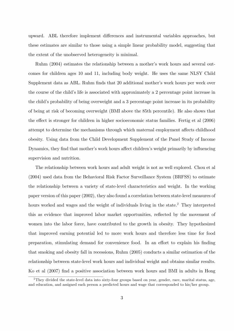
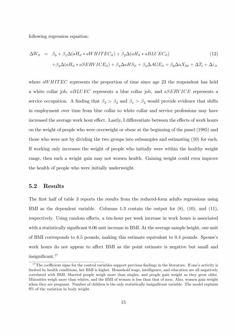
The fact that America�s weight gain has coincided with the increase in labor force par-

ticipation (see Figure 1) suggests that a causal relationship between these trends may be

1Children and adolescents are classi�ed as �overweight�if they have a BMI at or above the 95th percentilebased on age- and gender-speci�c growth charts. With children and adolescents, the term �obese� is usedinterchangeably with "overweight." Percentiles are determined using child BMI data from the second andthird National Health Examination Surveys (NHES II and NHES III) and from the �rst, second, and thirdNational Health and Nutrition Examination Surveys (NHANES I, NHANES II, and NHANES III). Thesesurveys spanned the period 1963-1994; therefore, the percentage of children who are overweight is not �xed at5%.

1

possible. In theory, an individual working more hours could limit available time for exercise,

causing her to gain weight. She could also devote less time to food preparation, causing a

substitution from home-prepared meals to less healthy convenience food, such as fast food

and pre-prepared processed food, resulting in a weight gain for herself as well as other family

members. Moreover, parents working could limit the amount of supervision their children

receive, allowing them to make less healthy eating and exercise decisions.

In this paper, I attempt to determine the relationship between adult work hours and the

weight of both adults and children. Applying di¤erencing methods to panel data from the

National Longitudinal Survey of Youth (NLSY) and NLSY Child Supplement (NLSYCS),

I �nd that an increase in a man or woman�s work hours increases the person�s own weight

and, to a lesser extent, the weight of his or her spouse. Employing an instrumental variables

approach, I show that this e¤ect occurs by reducing exercise and increasing the percentage

of the family�s food budget used to purchase food from restaurants. I also conclude that

mothers�, but not fathers�, work hours a¤ect the weight of children. Ultimately, I estimate

that changing employment patterns account for 6% of the rise in adult obesity between 1961

and 2004 and 10% of the increase in overweight children from 1968 to 2001.

2 Literature Review

Most of the literature on work hours and body weight focuses on the e¤ect of maternal

employment on childhood obesity. Using data from the NLSY matched with the NLSYCS,

Anderson, Butcher, and Levine (2003) (ABL) found that a mother working 10 additional hours

per week over the course of a child�s life (ages 3-11) is associated with a 1 percentage point

increase in the probability that the child is overweight. ABL argue that estimates of the work

hour e¤ect could su¤er from unobserved heterogeneity. Mothers who work may simply be those

who are less concerned with their children�s health, creating a spurious negative relationship.

On the other hand, ambitious mothers may both work and value health, biasing the e¤ect

2

upward. ABL therefore implement di¤erences and instrumental variables approaches, but

these estimates are similar to those using a simple linear probability model, suggesting that

the extent of the unobserved heterogeneity is minimal.

Ruhm (2004) estimates the relationship between a mother�s work hours and several out-

comes for children ages 10 and 11, including body weight. He uses the same NLSY Child

Supplement data as ABL. Ruhm �nds that 20 additional mother�s work hours per week over

the course of the child�s life is associated with approximately a 2 percentage point increase in

the child�s probability of being overweight and a 3 percentage point increase in its probability

of being at risk of becoming overweight (BMI above the 85th percentile). He also shows that

the e¤ect is stronger for children in higher socioeconomic status families. Fertig et al (2006)

attempt to determine the mechanisms through which maternal employment a¤ects childhood

obesity. Using data from the Child Development Supplement of the Panel Study of Income

Dynamics, they �nd that mother�s work hours a¤ect children�s weight primarily by in�uencing

supervision and nutrition.

The relationship between work hours and adult weight is not as well explored. Chou et al

(2004) used data from the Behavioral Risk Factor Surveillance System (BRFSS) to estimate

the relationship between a variety of state-level characteristics and weight. In the working

paper version of this paper (2002), they also found a correlation between state-level measures of

hours worked and wages and the weight of individuals living in the state.2 They interpreted

this as evidence that improved labor market opportunities, re�ected by the movement of

women into the labor force, have contributed to the growth in obesity. They hypothesized

that improved earning potential led to more work hours and therefore less time for food

preparation, stimulating demand for convenience food. In an e¤ort to explain his �nding

that smoking and obesity fall in recessions, Ruhm (2005) conducts a similar estimation of the

relationship between state-level work hours and individual weight and obtains similar results.

Ko et al (2007) �nd a positive association between work hours and BMI in adults in Hong

2They divided the state-level data into sixty-four groups based on year, gender, race, marital status, age,and education, and assigned each person a predicted hours and wage that corresponded to his/her group.

3

Kong with cross-sectional data. However, the study does not make an attempt to distinguish

between correlation and causality, and the authors write that "further studies are needed to

investigate the underlying mechanisms of this relationship . . . " (p. 254).

Lakdawalla and Philipson (2007) use NLSY panel data to study a related but di¤erent

question: how do the physical demands of one�s job a¤ect body weight? They show that

working at sedentary or strength-demanding (and therefore muscle-building) occupations is

associated with a higher weight than working at �tness-demanding occupations.

In this paper, I contribute to the literature primarily by providing a more complete analysis

of the link between work hours and adult weight. To my knowledge, this is the �rst paper

to estimate the e¤ect of individual-level work hours on adult body weight using panel data

to eliminate time-invariant sources of omitted variable bias in the estimates. I also provide

direct evidence that the work hour e¤ect occurs through the expected mechanisms: decreasing

exercise and inducing a substitution toward food prepared at restaurants. Additionally, I

di¤erentiate between work hour e¤ects on the basis of gender, marital status, spouse work

status, and employment sector. Finally, I show that work hours a¤ect only the weight of

individuals who are at risk for obesity, suggesting that the e¤ect of work hours on weight is

particularly hazardous to health.

My primary contribution to the childhood obesity literature lies in exploring the impact

of mothers�spouses�work hours, instead of only mothers�work hours, on child weight. In

response to increases in female employment, the percentage of adult men who work fell from

83% in 1950 to 73% in 2004 (Bureau of Labor Statistics, 2007). If men are perfect substitutes

for women in terms of child care, the e¤ect of more women working on the prevalence of

overweight children would be partially o¤set by the fact that more men stay at home. I also

contribute by utilizing a broader range of data than previous authors, as I include children

ages 3-17 as well as four more waves of NLSY data than ABL.

4

3 Analytical Framework

In this section, I develop a simple structural model of the e¤ect of work hours on adult body

weight, assuming that this e¤ect occurs through reducing exercise and inducing substitution

from home-cooked meals to food prepared outside the home. I de�ne the body mass index of

a representative agent as

BMIT = BMI0(S;R; I;G) +TXt=0

r(Ct �Bt) (1)

where BMI0 is a person�s initial BMI as determined by genetic factors such as sex (S), race

(R), natural intelligence (I), and other unobservable genetic attributes (G). A person�s change

in BMI in period t is equal to the di¤erence between her calories consumed (C) and burned

(B) in t, multiplied by the rate (r) at which this caloric balance is converted to units of

BMI. Therefore, BMI acts as a capital stock in that it depends on a person�s decisions in

all preceding periods.

People generally assume food prepared at restaurants to be, on average, less healthy than

food prepared at home. A variety of research �nds a positive correlation between frequency

of eating fast food and consumption of calories, fat, and saturated fat (for an example, see

Satia et al, 2004). Both the popular press and scholarly research have also criticized the

health quality of full-service restaurant meals, mainly for their increasingly large portions

(Young and Nestle, 2002) and use of hidden high-calorie �avor-enhancers such as butter and

oil ("Deadly Secrets ..."). Therefore, number of calories consumed depends on the percentage

of meals eaten out or delivered. Calories burned are a function of amount of exercise. Wage,

education, marital status, age, number of children, health limitations, and pregnancies may

also a¤ect body weight.3 I therefore model calories consumed and burned by the following

3In developed countries, earnings tend to be inversely related to BMI for most of the income distribution.This may be because healthy foods, such as fruits, vegetables, and lean meats, are more expensive than pre-prepared processed foods and other less healthy foods (Lakdawalla and Philipson, 2002). Education appearsto be inversely related to BMI, suggesting that schooling helps people to make more informed eating andexercise decisions (Nayga, 2001). Several papers suggest that BMI increases when people marry or grow older

5

equations:

Ct = C(Pt; Xt) (2)

Bt = B(Et; Xt) (3)

where X is a set of the aforementioned descriptive/demographic variables, P is the percentage

of meals prepared by restaurants, and E = amount of exercise.

If a person works more hours, she has less available time for exercise. Also, as previously

discussed, more work hours may increase P . Spouse�s work hours may also in�uence P , since

families often eat together. Spouse�s work hours do not impact exercise as clearly as own work

hours. However, an individual could potentially increase exercise if her spouse works more,

since spending less time with her spouse allows more time for exercise. Therefore,

Pt = P (Ht; HSt; Xt) (4)

Et = E(Ht; HSt; Xt) (5)

where H = hours worked and HS = spouse�s hours worked.

Combining (1), (4), and (5) yields the following structural model for adult BMI:

BMIT= BMI

"S;R; I;G;

TXt=0

��tBMICt(P (H t; HSt; X t; UPt); E(P (H t; HSt; X t; UEt); X t; UOt)

�#(6)

where BMIC is change in BMI, which is a function of the aforementioned variables plus

unobservable personal and societal characteristics UP , UE, and UO.

(for an example, see Rashad, 2006). BMI may rise as number of children increases, since additional childrenplace a constraint on time similar to that caused by additional work hours. Also, if a person is sick or injured,her level of physical activity may fall, increasing BMI. Finally, pregnancies increase the BMI of women.

6

I next convert (6) to a reduced-form model by substituting for P and E:

BMIT = BMI

"S;R; I;G;

TXt=0

��tBMICt(Ht; HSt; Xt; Ut)

�#(7)

where U captures all unobservable determinants of BMI changes.

In this paper, I estimate both the structural and reduced-form models. The structural

model is more informative, but relies on the assumption that work hours in�uence weight

only by a¤ecting exercise and the percentage of meals prepared away from home, which may

not be valid. First, additional work hours create additional income, which may reduce weight,

although previous estimates of the e¤ect of income on weight suggest that this e¤ect would

be small.4 More importantly, working more may leave less time for eating, causing weight to

fall. Also, working creates stress, which can lead to overeating and weight gain (Greeno and

Wing, 1994). The reduced-form model does not specify the way in which work hours a¤ect

weight, meaning that I allow all of these factors to have an impact.5

Developing a testable structural model for the e¤ect of parent work hours on child body

weight is di¢ cult since this e¤ect occurs through di¤erent channels than that on adult weight.

While substitution to food prepared outside the home should a¤ect child as well as adult

weight, much of the e¤ect on children is likely the result of changes in time spent with parental

supervision. Older children may be left unsupervised, and they may make less healthy eating

and exercise decisions than if their choices were monitored. Parents are less likely to leave

younger children alone, but baby-sitters and day-care workers may not value the long-term

health of a child as much as the child�s parent. The NLSYCS does not include data on child

supervision. Therefore, for children, I only estimate reduced-form models similar to (7).

4For example, Chou, Grossman, and Sa¤er�s (2004) results imply that, at the sample mean, a 10% increasein income would decrease BMI by 0.1%.

5Since I include hourly rate of pay as a control instead of income, the reduced-form model allows part ofthe e¤ect of work hours on weight to occur through changes in income.

7

4 Data

For regressions of adult body weight, I use data from the 1979 cohort of the National Longi-

tudinal Survey of Youth. The NLSY includes data from 6,111 randomly-chosen U.S. youths,

plus a supplemental sample of 5,295 minority and economically disadvantaged youths and

1,280 military youths. The NLSY �rst conducted interviews in 1979, and all respondents were

between fourteen and twenty-two years of age at this time. Subsequent interviews occurred

each year until 1994, and then every two years until 2004. The respondents�reported their

weight in 1981, 1982, 1985, 1986, 1988, 1989, 1990, 1992, 1993, 1994, 1996, 1998, 2000, 2002,

and 2004 and their height in 1981, 1982, and 1985. In order to ensure that my sample consists

entirely of adults, I include only the years 1985-2004. Given the age of respondents, I assume

height in 1985 to be adult height and use it as height for all years. Although the retention rate

of the NLSY79 was high, not all youths were followed for the duration of the sample; therefore,

my data are an unbalanced panel. Eliminating observations with missing data leaves me with

a total of 10,194 individuals and 85,759 observations. Table 1 reports summary statistics for

variables used in the adult regressions.

I obtained data on children from the NLSY79CS, which features interviews with chil-

dren of mothers found in the NLSY79. Children�s height and weight were only recorded in

even-numbered years from 1986-2004; therefore, these are the years included in my sample.

Following the approach of ABL, I drop children under the age of 3. I also eliminate those

over 17 since such young adults are less likely to live with their parents. Table 2 summarizes

the data taken from the NLSYCS. Other variables used in regressions of children�s weight are

information about the child�s mother matched from the NLSY.6 After eliminating observa-

tions with missing data, my sample size for children�s regressions is 33,652 observations (8,611

children).

The �rst dependent variable in my adult regressions is body mass index, which is equal to

6Since the NLSY generally interviewed mothers and their children at the same time, virtually all childrenin the NLSYCS lived with their mothers. Therefore, modeling their weight as a function of their mother�sattributes should be reasonable.

8

weight in pounds divided by height in inches squared, multiplied by 703. Following convention

in the literature, I also use a binary variable for whether or not the individual is obese. The

average BMI in the sample is 26.0, while the obesity rate is 17.9%. Using BMI for children

is inappropriate since the medically optimal BMI is di¤erent for children and young adults of

di¤erent ages. For example, a 10-year-old boy is overweight if his BMI is above 22, while a

15-year-old boy would not be overweight until his BMI reached 27. Therefore, for regressions

of child weight, my dependent variable is whether or not the child is overweight, which I

construct using age- and gender-speci�c CDC growth charts.7 Again, with children, the terms

"overweight" and "obese" are used interchangeably. 14.7% of the sample is overweight/obese.

My independent variables of interest are the person�s (child�s mother in children�s regressions)

average hours worked per week since the last interview and spouse�s average hours worked per

week in the past year, in units of 10. The sample means for hours and spouse�s work hours

are 3.4 and 2.2, respectively. The mean for spouse�s work hours is smaller because I impute

values of zero for single people.

For structural models of adults�weight, I construct an estimate of exercise frequency using

two survey questions. In 1998 and 2000, the NLSY asked the respondents the frequency with

which they obtained both light exercise, such as walking, and strenuous exercise, such as

working out or participating in sports. For both questions, the respondents chose from the

following options: never, less than once a month, one to three times a month, once or twice

a week, and three or more times a week. Using this information, I formed estimates of the

individuals�number of times exercising, both light and heavy, per week. If a person answered

"never," I assigned her a value of 0. Someone who answered "less than once a month" was

assigned a value of 1/8 time exercising per week (1/2 per month), while one to three times a

month was assigned 1/2 per week (2 per month), one to two times a week was assigned 1.5

7Self-reported weight and height could be problematic as people commonly underreport their weight and,to a lesser extent, overreport their height. However, researchers with access to both self-reported and actualweight and height have shown that, in regressions of body weight, correcting for errors in the self-reportedvalues does not substantially alter coe¢ cient estimates (for examples, see Cawley (1999) and Lakdawalla andPhilipson (2002)). In other words, the extent to which one underreports weight or overreports height does notappear to be correlated with the variables commonly included in body weight regressions.

9

per week, and three or more times a week was assigned 4 per week. I then added light and

heavy exercise to determine total exercise.8 Using this approach, the average individual in my

sample exercised 3.8 times per week.

Due to data limitations, I use proportion of total food expenses spent on restaurants as

a proxy for percentage of meals prepared away from the home. In the 1990-1994 surveys,

the NLSY asked respondents to estimate their total food expenditures as well as the amount

spent at restaurants and on food delivery. Adding the amounts spent at restaurants and

on delivery, then dividing this sum by total food expenditures, yields the proportion of food

expenses spent on food prepared by restaurants. For the average respondent, this number was

26%.

In some regressions, I also group hours worked by occupation type: blue collar, white

collar, or service. I consider an individual to be "blue collar" if her primary occupation is

classi�ed as "craftsman, foremen, and kindred;" "armed forces;" "operatives and kindred;"

"laborers, except farm;" "farmers and farm managers;" or "farm laborers and foremen." I

label an individual "white collar" if her occupation is "professional, technical, and kindred;"

"managers, o¢ cials, and proprietors;" "sales workers;" or "clerical and kindred" and "service"

if her occupation is "service workers, except private household" or "private household."

The wide range of questions asked by the NLSY survey allows me to include the other

factors discussed in section 3 that could be expected to in�uence adult weight: race, gender,

intelligence (score on the Armed Forces Qualifying Test), hourly rate of pay, highest grade

completed, marital status, age, number of children, whether or not the respondent has any

health conditions that limit the amount or type of work she can perform, and whether or not

the respondent is pregnant.9

8One might expect heavy exercise to reduce weight more than light exercise. However, strenuous exercisesuch as weightlifting builds muscle mass in addition to burning fat, so theoretically heavy exercise may actuallyhave a smaller overall impact on weight. Since I am uncertain about the relative impact of the two types ofexercise, I weight them equally.

9I construct hourly rate of pay for the household by dividing total household income by the sum of ownand spouse�s work hours (which are zero if the person is single). I set rate of pay to zero for householdswhere neither the respondent nor her spouse worked at all during the preceding year; this a¤ects a very smallpercentage of households.

10

For children�s weight, I include these same characteristics (except for pregnancy status) as

well as birth order and indicator variables for whether or not the child�s mother is overweight

or obese. I add these variables to mirror the approach used by ABL.

5 Reduced-Form Adults

5.1 Models

I begin by estimating the reduced-form model (7). The reduced-form approach captures the

overall e¤ect of work hours on weight, which may occur through several channels, whereas the

structural model forces this e¤ect to occur only through exercise and the percentage of food

prepared by restaurants. The discussion in section 3 highlights the importance of accounting

for past values, in addition to current values, of the independent variables. In their studies

of the e¤ect of maternal employment on child weight, ABL and Ruhm (2004) accomplish this

by converting the key independent variables to averages of their values over the child�s entire

life. Since I focus on adults, whom I do not observe from birth, I apply a variation of their

approach by averaging over the individual�s entire adult life, which I de�ne as being at least

23 years old.10 Assuming a linear functional form, I begin by estimating the following random

e¤ects model with generalized least squares:11

Wit = �0 + �1aHit + �2aHSit + �3AGEit + �4X1it + �5aX2it + Tt + !i + "it (8)

where Wit is a measure of weight (BMI or obesity status)12 for individual i in period t, H is

average weekly work hours in units of 10, HS is spouse�s average weekly work hours in units

10I use age 23 instead of 18 because individuals in the 18-22 age group are likely to be college students.Students may work a large number of hours, but the NLSY work hour statistics do not re�ect unpaid work,such as studying.11In order to estimate a random e¤ects model with sampling weights, I use the Stata module "xtregre2" by

Merryman (2005).12I estimate linear probability models (LPMs) when obesity status is the dependent variable. In the children�s

section, this makes my results comparable to those of ABL, who also used LPMs. All results are robust tothe use of probit and logit models.

11

of 10, X1 is a set of time-invariant controls (race, gender, and intelligence), X2 is a set of

controls (other than age) that vary over time (marital status, health limitations, hourly rate

of pay, education, number of children, and whether or not the person is pregnant), T is a year

�xed e¤ect, and ! is the random e¤ect. Also, a indicates average, which I de�ne as

aZit =

tPj=1

Zij �WKij

tPj=1

WKij

(9)

where Z = H; HS; or X2 and WKij is the number of weeks since the respondent�s last

interview (or 52 for the �rst interview). I do not average age, pregnancy status, the time-

invariant characteristics in X1, and the time dummies. �1 measures the e¤ect of an additional

ten work hours per week over the individual�s entire adult life on BMI or P(Obese), while �2

measures the e¤ect of one�s spouse working an additional ten hours. I set spouse�s work hours

equal to 0 if the person is single. By controlling for marital status, I di¤erentiate between the

e¤ect on single people and married people whose spouses do not work.

In the random e¤ects model, b�1 and b�2 are consistent only if the individual e¤ect �i isuncorrelated with work hours and spouse�s work hours, an assumption that may not be valid.

For example, people who are ambitious may both work a large number of hours and maintain

a healthy weight, biasing b�1 downward. Since people tend to choose spouses who are similarto themselves, the estimates of �2 could also su¤er from bias. Additionally, hard-working,

�nancially successful individuals may marry thin spouses, in which case b�2 may be biaseddownward.

To account for sources of endogeneity that are constant over time, ABL use a "long dif-

ferences" approach in which they di¤erence between the child�s last and �rst years in the

sample.13 Because they used children in the age range 3-11, the di¤erences for most children

were over an eight-year period. Since weight likely responds gradually to changes in work

13Since the independent variables of interest are averages over the child�s life, di¤erences re�ect changes inthe variable averages over time.

12

hours, such an approach may be more appropriate than �rst di¤erences or �xed e¤ects. ABL

also argue that long di¤erencing reduces the extent of bias from measurement error.

In order to apply a similar estimation technique to adults, I di¤erence between the current

year and eight years ago. Since most adults are in the sample for twenty years, di¤erencing

between the last and �rst years may be excessive in accounting for the gradual nature of weight

changes. Also, by allowing each individual to be in the sample more than once, I retain the

degrees of freedom and extra information from the additional observations.14 I restrict the

sample to observations where the person was at least 28 years old in the initial period. This

ensures that the averages in each initial period are based on at least �ve years�worth of data,

and therefore not driven by one atypical year.15

My long di¤erence regression equation is:

�Wit = �0 + �1�aHit + �2�aHSit + �3�AGEit + �4�aX2it +�Tt +�"it (10)

where � represents di¤erence. b�1 and b�2 now provide consistent estimates under the assump-tion that changes in work hours are uncorrelated with changes in the error term. While I

cannot be completely certain of the validity of this assumption, the most likely sources of

bias, such as ambition, are relatively stable over time. Also, failure to account for changes

in ambition over time should bias my estimates downward, in which case my results are a

lower bound.16 Furthermore, ABL employed both long di¤erences and instrumental variable

approaches, and obtained similar results with each, suggesting that di¤erencing produces a

consistent estimate of the e¤ect of maternal work hours on child weight. Nonetheless, I cannot

be sure that these �ndings would be similar with adult weight.

(8) and (10) both assume that the e¤ect of one�s work hours on weight is the same for

14In regressions not reported in this paper, I di¤erence between the last and �rst years and obtain verysimilar results.15Results are robust to starting at a di¤erent age.16I cannot completely rule out the possibility that my estimates are biased upward. For example, people

who work long hours may be those who are less concerned about their health than others and therefore weighmore.

13

both married and single people. However, people who are married have a spouse to assist

with meal preparation; therefore, the work hour e¤ect may be smaller for them than for

singles. Alternatively, marrying often introduces a new set of responsibilities, ranging from

home ownership to raising children. If married individuals face tighter time constraints than

singles, marrying may exacerbate the work hour e¤ect.

In (8) and (10), I also assume that the e¤ect of one�s work hours on weight does not depend

on how much one�s spouse works, and that the e¤ect of spouse�s work hours on weight does

not depend on own work hours. If a person whose spouse does not work begins to work more,

the spouse may be able to compensate by handling more of the food preparation duties. If the

spouse also works, this becomes more di¢ cult, suggesting that the work hour e¤ect depends

on spouse�s work hours, and (analogously) that the spouse work hour e¤ect depends on own

work hours.

I next relax these assumptions by interacting work hours with marital status and spouse�s

work hours:

�Wit = �0 + �1�aHit + �2�aHSit + �3�(aHWKit � aUNMARRIEDit) (11)

+�4�(aHit � aHSit) + �5�AGEit + �6�aX2it +�Tt +�"it

The e¤ect of ten additional work hours per week is �1 + �3 for singles, �1 for married

people whose spouses do not work, and �1 + 4�4 for married people whose spouses work 40

hours per week. The spouse work hour e¤ect is �2 for people who do not work and �2 + 4�4

for those who work 40 hours per week.

In my �nal reduced-form regressions for adults, I conduct additional tests of the homo-

geneity of the work hour and spouse�s work hour e¤ects. First, I estimate (10) separately for

men and women to determine if these e¤ects vary on the basis of gender. Next, I di¤erenti-

ate between the work hour e¤ects of white collar, blue collar, and service workers using the

14

following regression equation:

�Wit = �0 + �1�(aHit � aWHITECit) + �2�(aHit � aBLUECit) (12)

+�3�(aHit � aSERV ICEit) + �4�aHSit + �5�AGEit + �6�aX2it +�Tt +�"it

where aWHITEC represents the proportion of time since age 23 the respondent has held

a white collar job, aBLUEC represents a blue collar job, and aSERV ICE represents a

service occupation. A �nding that �3 > �2 and �1 > �2 would provide evidence that shifts

in employment over time from blue collar to white collar and service professions may have

increased the average work hour e¤ect. Lastly, I di¤erentiate between the e¤ects of work hours

on the weight of people who were overweight or obese at the beginning of the panel (1985) and

those who were not by dividing the two groups into subsamples and estimating (10) for each.

If working only increases the weight of people who initially were within the healthy weight

range, then such a weight gain may not worsen health. Gaining weight could even improve

the health of people who were initially underweight.

5.2 Results

The �rst half of table 3 reports the results from the reduced-form adults regressions using

BMI as the dependent variable. Columns 1-3 contain the output for (8), (10), and (11),

respectively. Using random e¤ects, a ten-hour per week increase in work hours is associated

with a statistically signi�cant 0.06 unit increase in BMI. At the average sample height, one unit

of BMI corresponds to 6.5 pounds, making this estimate equivalent to 0.4 pounds. Spouse�s

work hours do not appear to a¤ect BMI as the point estimate is negative but small and

insigni�cant.17

17The coe¢ cient signs for the control variables support previous �ndings in the literature. If one�s activity islimited by health conditions, her BMI is higher. Household wage, intelligence, and education are all negativelycorrelated with BMI. Married people weigh more than singles, and people gain weight as they grow older.Minorities weigh more than whites, and the BMI of women is less than that of men. Also, women gain weightwhen they are pregnant. Number of children is the only statistically insigni�cant variable. The model explains9% of the variation in body weight.

15

As shown in column (2), di¤erencing increases the estimated work hour and spouse�s work

hour e¤ects substantially. A ten-hour per week increase in a person�s work hours increases

her BMI by 0.18 units (1.2 pounds) at the sample mean height, while a similar increase in

spouse�s work hours leads to a 0.1 unit rise in BMI (0.7 pounds). These results suggest that

those obtained using random e¤ects were biased downward, which is not surprising given the

discussion in the preceding section.

The third column shows the regression output when I include the interaction terms aH �

aUNMARRIED and aH � aHS. The work hour e¤ect is weaker for people who are single,

implying that the e¤ect of facing additional constraints on time after marrying outweighs the

e¤ect of having an additional person to share with the food preparation. The interaction term

work hours*spouse�s work hours is positive, as expected. However, neither interaction term

is signi�cant, so these �ndings are inconclusive. The �rst column of tables 4 and 5 expresses

these results in a more usable form. The e¤ect of 10 additional work hours over an individual�s

entire adult life is 0.4 pounds for singles, 1.3 pounds for people who are married to a spouse

who does not work, and 1.8 pounds for people who are married to a spouse who works. The

e¤ect of 10 additional spouse�s work hours is 0.3 pounds for people who do not work and 0.8

pounds for people who work.

The second half of table 3 reports the results using whether or not the person is obese

as the dependent variable. Signs of the coe¢ cients are similar to those using BMI. With

random e¤ects, work hours increase P(Obese) by 0.7 percentage points while spouse�s work

hours decrease it by 0.6 percentage points. Both variables are signi�cant in both regressions.

Applying long di¤erences, working ten additional hours per week increases one�s P(Obese) by

a statistically signi�cant 1.2 percentage points. The spouse work hour e¤ect becomes virtually

zero, suggesting that spouse�s work hours may a¤ect weight but not obesity.

The sign of the coe¢ cient of the interaction term unmarried*work hours is again negative,

while that of work hours*spouse�s work hours is now negative but very small. Both are

statistically insigni�cant. The second column of tables 4 and 5 shows that the e¤ect of

16

10 additional work hours per week on the probability of becoming obese is 0.8 percentage

points for singles, 2.0 percentage points for married people with non-working spouses, and 1.5

percentage points for married people with working spouses. The spouse work hour e¤ect is

0.4 percentage points for those who do not work and -0.1 percentage points for those who do.

Table 6 shows the results for the regressions which divided the sample into women and

men. Since the impact of adding the interaction terms was inconclusive, I use long di¤erences

without interaction terms. The work hour e¤ect appears stronger for women than men when

using BMI as the dependent variable, but becomes stronger for men when obesity status is

used. Neither di¤erence is statistically signi�cant at the 5% level. For both genders, one�s

spouse working causes a modest increase in BMI but essentially no change in P(Obese). In

short, there does not appear to be an obvious di¤erence in how own or spouse�s work hours

impact the weight of the two genders.

In table 7, I report results for the regressions with work hours grouped by occupation type.

The work hour e¤ect does appear strongest for white-collar workers, but the e¤ect on blue-

collar workers is almost as large. Only service workers do not appear a¤ected by additional

work. When interpreting these �ndings, note that BMI does not distinguish between fat and

muscle mass. It is possible that blue-collar workers, who often engage in strenuous on-the-job

exercise, may actually be adding muscle instead of fat. In contrast, the jobs of service workers

likely involve only low-intensity exercise, such as walking, which builds little or no muscle. If

the weight gain of blue-collar workers is in fact muscle instead of fat, then my results may

overstate the health consequences of additional work.

Table 8 displays the results dividing the sample into people who were overweight or obese

at the beginning of the panel, whom I classify as "at risk" for obesity, and those who were not.

The e¤ects of own and spouse�s work hours on the BMI of the "at risk" group are positive

and large. The own work hour e¤ect implies that an unemployed person who begins to work

forty hours per week will ultimately gain almost ten pounds. However, the e¤ects on the BMI

of people who did not begin the panel overweight are small and insigni�cant. One possible

17

explanation for the discrepancy is that people who place a high value on health may make

a special e¤ort to maintain healthy eating and exercise habits after their work hours rise.

For example, they may still eat more fast food but choose the healthiest items on the menu.

However, it is also possible that all people make less healthy decisions, but only those who are

genetically prone to weight gain actually gain a noticeable amount of weight. In either case,

the fact that the impact of work hours on weight is substantially stronger for people who are

at risk for obesity means that the work hour e¤ect is particularly hazardous to public health.

6 Structural Estimation

6.1 Model

I next estimate the structural model (6) to determine if work hours a¤ect exercise and eating

at restaurants, and if exercise and eating at restaurants a¤ect weight. I employ a two-stage

least-squares procedure, using work hours and spouse�s work hours as instruments for exercise

and percentage of food expenditures spent on restaurants. Since spouse�s work hours are only

non-zero for people who are married, I drop singles from the sample. My regression equations

are

\PREST it = 0+ 1Hit+ 2HSit+ 3AGEit+ 4X1it+ 5X2it+ 6t+ �it (13)

\EXERCISEit = �0+�1Hit+�2HSit+�3AGEit+�4X1it+�5X2it+�5t+ �it (14)

Wit = �0+�1 \PREST it+�2 \EXERCISEit+�3AGEit+�4AGEit (15)

+�5X1it+�6X2it+�7t+ �it

where PREST is the percentage of one�s family�s food expenditures spent on restaurants

and EXERCISE is the average number of times exercising per week. In the �rst-stage

regressions (13) and (14), I estimate the determinants of PREST and EXERCISE. I use

these predicted values in the second-stage regression (15). I elect not to employ a di¤erences

18

approach because it would result in the loss of half the sample for (14), in�ating the standard

errors to the point where H and HS become very weak instruments for EXERCISE.18 In

the reduced-form section, neglecting to di¤erence biased my results downward. I therefore

expect that, if anything, the results in this section are understatements.

My estimates of �1 and �2 are consistent if and only if H and HS are uncorrelated with �,

which may not be the case if the work hour e¤ect occurs partially through other mechanisms.

The second-stage estimates should therefore be interpreted with caution. However, the �rst-

stage estimates of the e¤ect of work hours and spouse�s work hours on exercising and eating

are the primary focus of this section, since the second-stage �ndings that exercise reduces

weight and that eating at restaurants increases weight are already widely assumed.

Another limitation of the structural analysis is that PREST is available in only �ve surveys

(1990-1994), while exercise data is reported in only two (1998 and 2000). Consequently,

estimating (15) with only the years used to estimate (13) and (14) results in no observations.

I therefore generate predicted values for PREST and EXERCISE in all years of the panel

using only the data from the years in which the variables are de�ned. The validity of this

approach depends on if the relationships between the regressors in (13) and PREST are the

same in 1990-1994 as they are in the other survey years, and the relationships between the

regressors in (14) and EXERCISE are the same in 1998-2000 as they are in the other survey

years.19 I compute bootstrap standard errors in both stages.

The relationship between work hours and income creates an additional complication. Since

I control for wage instead of income in (13)-(15), income is an omitted variable. Working

additional hours increases income, which decreases weight, so my estimates of �1 and �2 will

likely be biased toward zero. However, a variety of research shows that the e¤ect of income on

weight is small (see footnote 3), so I expect that the extent of the bias is minimal. Nonetheless,

18Di¤erencing does not a¤ect the results in (13), likely because PREST exists in �ve survey waves, comparedto only two for EXERCISE.19Since year �xed e¤ects cannot be used with this approach, I include a linear time trend instead. In

the reduced-form analysis, using a linear time trend instead of year e¤ects does not substantially change theresults.

19

as a robustness check I also estimate the two-stage least-squares model including income as a

control instead of wage.

6.2 Results

Table 9 shows the results for the �rst stage of the two-stage least-squares analysis. The �rst two

columns estimate the determinants of the percentage of household food expenditures spent on

food prepared at restaurants, while the third and fourth columns estimate the determinants

of exercise frequency. Columns labeled (1) include wage as a control, while those labeled

(2) include income. As expected, the two sets of results are very similar. A ten-hour per

week increase in work hours increases the proportion of food prepared at restaurants by a

statistically signi�cant 0.9-1.0 percentage points (4%), and the spouse work hour e¤ect is

virtually identical.20

As expected, additional work hours decrease exercise. A ten-hour per week increase is

associated with a statistically signi�cant 0.10-0.11 fewer times exercising per week (3%).21

Interestingly, spouse�s work hours are positively correlated with exercise. While the e¤ect is

small, it is signi�cant at the 10% level. One possible explanation for this result is that, if one

spends less time with one�s spouse, more time becomes available for other activities, such as

exercising.22

Table 10 reports the results for the second stage. The predicted values of percentage of

food prepared by restaurants and exercise have the expected e¤ect on BMI and P(Obese). A

10 percentage point, or 40%, increase in proportion of food prepared by restaurants increases

BMI by 0.26-0.32 units and P(Obese) by 2.5-3.4 percentage points (14-19%). Exercising one

additional time per week is associated with a 0.8 unit reduction in BMI and 5.4-5.5 percentage

20Health limitations, age, number of children, intelligence, and being pregnant are negatively associatedwith this proportion, while household wage and education are positively associated with it.21Results are almost identical using a Tobit model left-censored at 0, as less than 5% of the sample reports

never exercising.22Health limitations appear to decrease exercise, while education and intelligence increase it. The e¤ects of

wage, age, number of children, and pregnancy status are inconclusive. Blacks exercise less than whites, whilewomen exercise less than men.

20

point drop in P(Obese) (30%). Both exercise and percentage of food prepared at restaurants

are statistically signi�cant.

Tables 11 and 12 combine the �rst and second stages to determine the overall e¤ect of

work hours on weight. Working an additional ten hours per week increases BMI by 0.11-0.12

units (0.7-0.8 pounds) and P(Obese) by 0.8-0.9 percentage points. The e¤ect of spouse�s

work hours is essentially zero. These magnitudes are similar to those obtained using pooled

OLS reduced-form estimation. Approximately 30% of this work hour e¤ect occurs through a

substitution away from food prepared at home to food prepared at restaurants, while the other

70% occurs through reducing exercise. Spouse�s work hours do not appear to a¤ect weight:

the food substitution e¤ect is o¤set by the increase in exercise. As expected, the e¤ects of

work hours on weight are slightly larger when I control for income instead of wage.

7 Reduced-Form Children

7.1 Models

I next analyze the e¤ect of parents�work hours on the weight of children and young adults.

I employ only reduced-form models since, as shown by Fertin et al (2006), much of the e¤ect

of work hours on child weight occurs through changes in supervision, which I do not observe

in the data. My estimation approach for children is virtually identical to that of ABL, except

for three main changes. First, they only utilize up to the 1996 NLSY wave, so my data set

includes an additional four periods. Second, I include mother�s spouse�s work hours as a

regressor in addition to mother�s work hours. Third, my sample consists of all children and

young adults between the ages of 3 and 17, whereas their sample excludes those over 11.

I begin with a random e¤ects linear probability model with the independent variables

converted to averages over the child�s entire life, using whether or not the child is overweight

21

(O) as the dependent variable:

Oit = �0+�1aHit+�2aHSit+�3aAGEit+�4aCHAGEit+�5X1it+�6aX2it+!i+Tt+"it (16)

where AGE is the child�s mother�s age, while CHAGE is the child�s age. X1 again represents

the set of time-invariant characteristics, which in this case are mother�s intelligence and child�s

race, gender, and birth order. X2 is the set of characteristics that vary over time: mother�s

household wage, education, marital status, overweight status, and obesity status and the

total number of children under the age of 18 living in the child�s home. I again construct

independent variable averages according to equation (9).

I next implement a long di¤erences approach, using the child�s �rst observation after

turning three as the "initial period," and her last observation before turning eighteen as the

"�nal period." Few children are in the sample from birth to the age of eighteen; the average

length of time between initial and �nal periods is seven years. Next, I include the interaction

terms H �UNMARRIED and H �HS. Finally, I conduct separate regressions for boys and

girls to determine if the work hour e¤ect di¤ers on the basis of the child�s gender.

7.2 Results

In table 13, I report the results from the regressions of children�s probability of being over-

weight. Columns (1) to (3) show regression output from estimating the random e¤ects model,

the long di¤erences model, and the long di¤erences model with the interaction terms, respec-

tively. In the �rst column, ten additional mother�s work hours per week over the course of the

child�s life are associated with a 0.8 percentage point increase in P(Overweight), but the e¤ect

of spouse�s work hours is practically zero.23 Long di¤erencing doubles the mother�s work hour

e¤ect, but the spouse work hour e¤ect remains essentially zero.

23Mother�s education and intelligence and the number of children in the household are negatively correlatedwith children�s P(Overweight). P(Overweight) rises if the child is black or the mother is older, overweight,or obese. Female children are less likely to be overweight than male children. The other variables are notstatistically signi�cant.

22

Column 3 shows that the work hour e¤ect is slightly stronger for children of unmarried

mothers, and slightly weaker for children of married mothers whose spouses work. Both

interaction terms are insigni�cant. Tables 14 and 15 o¤er a more useful display of these

results. The impact of a mother working an additional 10 hours per week on her child�s

P(Overweight) is 2.5 percentage points for single mothers, 1.8 percentage points for married

mothers whose husbands do not work, and 1.4 percentage points for married mothers whose

husbands work. If a mother�s spouse works an additional 10 hours per week, her child�s

P(Overweight) rises by 0.3 percentage points if the mother works and falls by 0.1 percentage

points if she does not.

Table 16 displays the coe¢ cients of interest for the regressions where I divide the sample

into girls and boys. The results are very similar for the two genders.

8 Economic Signi�cance

I next examine the economic signi�cance of these results by attempting to answer two ques-

tions. First, what would be the e¤ect of a ten-hour-per-week increase in all adults�work hours

on the prevalence of obesity and overweight children, mortality, and medical expenditures?

Second, what percentage of the increase in adult obesity and overweight children over the past

half-century can be explained by observed changes in the employment patterns of men and

women?

In Appendix A, I describe in detail the method used to determine the answers to these

questions, and discuss possible caveats. I estimate that a ten-hour-per-week increase in the

average adult�s work hours would increase obesity by 3.7%, leading to 4,144 deaths and $4.33

billion in additional medical expenses per year. Adding ten hours to the work week for women

would increase childhood obesity by 11.1%. However, a similar increase in men�s work hours

would only increase childhood obesity by 0.6%. As displayed in table 16, observed changes in

employment patterns explain 6.2% of the rise in adult obesity during the period 1961 to 2004

23

and 10.4% of the rise in overweight children between 1968 and 2001.

9 Conclusion

In this paper, I analyze the e¤ect of adult work hours on the weight of both adults and children.

I �nd that adults who increase work hours exercise less and substitute from food prepared at

home to food prepared at restaurants, both of which lead to weight gain. An increase in a

person�s work hours leads to a smaller weight gain for her spouse; the food substitution e¤ect

appears to be o¤set by a slight rise in the spouse�s exercise. I also show that, if a mother

works more, the probability that her children and young adults are overweight rises. However,

mother�s spouse�s work hours do not a¤ect the weight of children, suggesting that mothers

pay more attention to the eating and exercise habits of their children than fathers. In the past

half-century, female employment in the U.S. has risen while male employment has fallen by a

lesser amount. I estimate that these changing employment patters account for 6% of the rise

in adult obesity between 1961 and 2004 and 10% of the increase in overweight children from

1968 to 2001. While these calculations are crude in that I extrapolate results obtained from

1985-2004 data to a longer time period, they suggest that the contribution of the increase in

labor force participation to America�s rise in obesity has been nontrivial.

Anecdotal evidence suggests that many Americans are working longer hours than ever,

and that employees in some professions routinely work sixty to eighty hours per week or more.

My results also imply that such long work weeks could have a detrimental e¤ect on health by

leading to a higher probability of becoming obese.

The results of this study should not be interpreted to mean that the increase in women�s

labor force participation has harmed society, or that women today should reduce their work

hours. The expansion of women�s rights that contributed to this rise in female employment was

obviously one of the great advancements of the 20th Century. My �ndings instead indicate that

people who work long hours should realize the potential health consequences and take steps

24

to prevent them from occurring. Government information-spreading programs may therefore

prove useful. Another possible policy implication is that the government could subsidize

"healthy" convenience food. Health bars and shakes, which require little or no preparation

time, are becoming commonplace in supermarkets and even convenience stores. However, they

remain expensive compared to less-healthy snack foods. Additionally, the government could

use tax incentives to encourage fast-food restaurants to serve a wider variety of healthy items.

Finally, tax incentives for companies to provide on-the-job exercise facilities would limit the

time costs associated with exercise and possibly mitigate the work hour e¤ect. Future research

is necessary to determine if any of these policies would improve social welfare.

25

References

Anderson P., Butcher K., and Levine P., 2003. �Maternal employment and overweight chil-dren.�Journal of Health Economics 22: 477-504.

Bureau of Labor Statistics, 2007. "Labor Force Statistics from the Current Population Survey."Available http://data.bls.gov/PDQ/outside.jsp?survey=ln.

Cawley J., 1999. "Addiction and the Consumption of Calories: Implications for Obesity."Working paper.

Chou S., Rahsad I., and Grossman M., 2006. "Fast Food Restaurant Advertising on Televisionand its E¤ect on Childhood Obesity." National Bureau of Economic Research Working Paper11879.

Chou S., Grossman M., and Sa¤er H., 2002. "An Economic Analysis of Adult Obesity: Re-sults from the Behavioral Health Factor Surveillance System." National Bureau of EconomicResearch Working Paper 9247.

Chou S., Grossman M., and Sa¤er H., 2004. "An Economic Analysis of Adult Obesity: Resultsfrom the Behavioral Health Factor Surveillance System." Journal of Health Economics, 23,565-587.

Courtemanche C., 2007. "Rising Cigarette Prices and Rising Obesity: Coincidence or Unin-tended Consequence?" Working paper, Washington University in St. Louis.

Cutler D., Glaeser E., and Shapiro J., 2003. "Why Have Americans Become More Obese?"Journal of Economic Perspectives, 17:3, 93-118.

Czajka-Narins D. and Parham E., 1990. "Fear of Fat: Attitudes Toward Obesity; the Thinningof America." Nutrition Today, Feb. 1990.

"Deadly Secrets of the Restaurant Trade," 2007. Reader�s Digest web site, availablehttp://www.rd.com/content/deadly-secrets-of-the-restaurant-trade.

Fertig A., Glomm G., Tchernis R., 2006. "The Connection Between Maternal Employmentand Childhood Obesity: Inspecting the Mechanisms." Working paper, Center for AppliedEconomics and Policy Research, Indiana University.

Finklestein E., RuhmC., and Kosa K., 2004. "Economic Causes and Consequences of Obesity."Annual Review of Public Health, 26, 239-257.

Flegal K., Carroll M., Kuczmarski R., and Johnson C., 1998. "Overweight and Obesity in theUnited States: Prevalence and Trends, 1960-1994." International Journal of Obesity 22(1):39-47.

Frank L., Andresen M., and Schmid T., 2004. "Obesity Relationships with Community Design,Physical Activity, and Time Spent in Cars." American Journal of Preventive Medicine 27(2):87�96.

26

Greeno C. and Wing R., 1994. "Stress-Induced Eating." Psychological Bulletin 115(3): 444-464.

Hedley A., Ogden C., Johnson C., Carroll M., Curtin L., and Flegal K., 2004. "Overweight andObesity Among U.S. Children, Adolescents, and Adults, 1999-2002." Journal of the AmericanMedical Association 291:2847-50. 2004.

Ko G. et al, 2007. "Association between Sleeping Hours, Working Hours and Obesity in HongKong Chinese: the �Better Health for Better Hong Kong�Health Promotion Campaign."International Journal of Obesity 31: 254�260.

Lakdawalla D. and Philipson T., 2002. "The Growth of Obesity and Technological Change:A Theoretical and Empirical Examination." National Bureau of Economic Research, workingpaper 8946.

Lakdawalla D. and Philipson T., 2007. "Labor Supply and Weight." Journal of Human Re-sources XLII(1): 85-116.

Merryman S., 2005. "Stata Module to Calculate Random E¤ects with Weights." Availablehttp://ideas.repec.org/c/boc/bocode/s456514.html.

Nakosteen R., Zimmer M., 2001. "Spouse Selection and Earnings: Evidence of Marital Sort-ing." Economic Inquiry 39(2): 201-13.

Nayga R., 2001. "E¤ect of Schooling on Obesity: Is Health Knowledge a Moderating Factor?"Education Economics, 9, 129-37.

Ogden C., Carroll M., Curtin L., McDowell M., Tabak C., and Flegal K., 2006. "Prevalence ofOverweight and Obesity in the Unived States, 1999-2004." Journal of the American MedicalAssociation 295: 1549-1555.

Ruhm C., 2005. "Healthy Living in Hard Times." Journal of Health Economics 24(2): 341-363.

Philipson T. and Posner R., 1999. "The Long-Run Growth in Obesity as a Function of Tech-nological Change." National Bureau of Economic Research, working paper 7423.

Ruhm C., 2004. "Maternal Employment and Adolescent Development." National Bureau ofEconomic Research Working Paper 10691.

Satia J., Galanko J., and Siega-Riz A., 2004. "Eating at Fast-food Restaurants is Associ-ated with Dietary Intake, Demographic, Psychosocial and Behavioural Factors among AfricanAmericans in North Carolina." Public Health Nutrition 7:1089-1096.

Strum R., 2002. "The E¤ects of Obesity, Smoking, and Drinking on Medical Problems andCosts." Health A¤airs 21: 245-53.

Young L., Nestle M., 2002. "The Contribution of Expanding Portion Sizes to the U.S. ObesityEpidemic." American Journal of Public Health, 92:246-249.

27

Appendix A �Economic Signi�cance Calculations

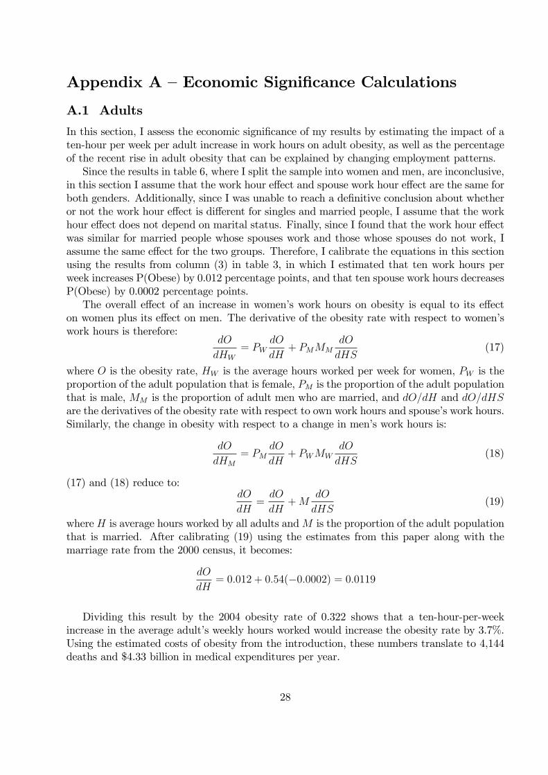
A.1 Adults

In this section, I assess the economic signi�cance of my results by estimating the impact of aten-hour per week per adult increase in work hours on adult obesity, as well as the percentageof the recent rise in adult obesity that can be explained by changing employment patterns.Since the results in table 6, where I split the sample into women and men, are inconclusive,

in this section I assume that the work hour e¤ect and spouse work hour e¤ect are the same forboth genders. Additionally, since I was unable to reach a de�nitive conclusion about whetheror not the work hour e¤ect is di¤erent for singles and married people, I assume that the workhour e¤ect does not depend on marital status. Finally, since I found that the work hour e¤ectwas similar for married people whose spouses work and those whose spouses do not work, Iassume the same e¤ect for the two groups. Therefore, I calibrate the equations in this sectionusing the results from column (3) in table 3, in which I estimated that ten work hours perweek increases P(Obese) by 0.012 percentage points, and that ten spouse work hours decreasesP(Obese) by 0.0002 percentage points.The overall e¤ect of an increase in women�s work hours on obesity is equal to its e¤ect

on women plus its e¤ect on men. The derivative of the obesity rate with respect to women�swork hours is therefore:

dO

dHW= PW

dO

dH+ PMMM

dO

dHS(17)

where O is the obesity rate, HW is the average hours worked per week for women, PW is theproportion of the adult population that is female, PM is the proportion of the adult populationthat is male, MM is the proportion of adult men who are married, and dO=dH and dO=dHSare the derivatives of the obesity rate with respect to own work hours and spouse�s work hours.Similarly, the change in obesity with respect to a change in men�s work hours is:

dO

dHM= PM

dO

dH+ PWMW

dO

dHS(18)

(17) and (18) reduce to:dO

dH=dO

dH+M

dO

dHS(19)

where H is average hours worked by all adults andM is the proportion of the adult populationthat is married. After calibrating (19) using the estimates from this paper along with themarriage rate from the 2000 census, it becomes:

dO

dH= 0:012 + 0:54(�0:0002) = 0:0119

Dividing this result by the 2004 obesity rate of 0.322 shows that a ten-hour-per-weekincrease in the average adult�s weekly hours worked would increase the obesity rate by 3.7%.Using the estimated costs of obesity from the introduction, these numbers translate to 4,144deaths and $4.33 billion in medical expenditures per year.

28

I next estimate the percentage of the increases in adult obesity (from 1961-2004) that canbe explained by changes in work hours during the periods.24 The proportion of adults whoare obese because of women�s work hours (OHW ) in period t is simply dO=dHW multiplied bythe average hours worked by women in t:

OHWt = HWtdO

dHW(20)

I approximate average weekly work hours for adult women using the percentage of single andmarried women employed part- and full-time combined with the average work hours for part-and full-time workers:

HWt = WSt(SWFtHF + SWPtHP ) +WMt(MWFtHF +MWPtHP ) (21)

where t is 1961 or 2004, WS is the proportion of women who are single, SWF is the proportionof single women who are employed full time, HF is the average weekly work hours (in unitsof 10) for full-time employees, SWP is the proportion of single women who are employed parttime, HP is the average weekly work hours for part-time employees, and married (M) replacessingle in the second half of the expression. Combining (17), (20), and (21), I obtain:

OHWt = [WSt(SWFtHF + SWPtHP ) +WMt(MWFtHF +MWPtHP )]�PW

dO

dH+PMMM

dO

dHS

�(22)

The equation for men is analogous. Calibrating the parameters using data from the CurrentPopulation Survey yields the following set of equations:25

OHW;1961 = [(0.34)(0.34*4.48+0.11*2.15)+0.66(0.23*4.48+0.08*2.15)] [0.53*0.012+0.47*0.69*-0.0002]

= 0:009

OHM;1961 = [(0.31)(0.49*4.48+0.04*2.15)+0.69(0.83*4.48+0.07*2.15)] [0.47*0.012+0.53*0.66*-0.0002]

= 0:019

OHW;2004 = [(0.49)(0.40*4.48+0.14*2.15)+0.51(0.43*4.48+0.15*2.15)] [0.52*0.012+0.48*0.56*-0.0002]

= 0:023

OHW;1961 = [(0.44)(0.55*4.48+0.07*2.15)+0.56(0.67*4.48+0.08*2.15)] [0.48*0.012+0.52*0.51*-0.0002]

= 0:017

Between 1960 and 2004, the adult obesity rate rose by 19.4 percentage points. The percentagesof this rise explained by changes in female and male employment patterns are:

OHW;2004 �OHW;19610:194

� 100% = 7:2% andOHM;2004 �OHM;1961

0:194� 100% = �1:0%

Therefore, the rise in female employment accounted for 7.2% in the rise in adult obesity

24The initial period was actually 1960-62, so I use the midpoint.251960 marriage rates are taken from the 1960 census.

29

between 1961 and 2004, while the concurrent drop in male employment o¤set about one-seventh of this increase. In total, changes in work hours accounted for 6.2% of the rise inobesity during the period.

A.2 Children

I next conduct a similar analysis for children. Given the lack of conclusive results when addingthe interaction terms and splitting the sample into girls and boys, in this section I assume thatthe work hour e¤ect is the same for girls and boys, as well as children of single and marriedmothers and children of married mothers whose husbands work and married mothers whosehusbands do not work. Therefore, I calibrate the equations in this section using the resultsfrom the third column of table 12. The e¤ect of a mother working ten hours per week on herchildren�s P(Overweight) is 0.016, while the e¤ect for the mother�s spouse is 0.001.The following equation expresses the change in the percentage of children who are over-

weight if women�s work hours increase by ten per week:

dOCdHW

= PCWdOCdH

(23)

where OC is the proportion of children who are overweight, PCW is the proportion of childrenwho live with their mothers (or another female guardian), and dOC=dHWK is the changein the "overweight rate" of children who live with their mothers with respect to a change inwomen�s work hours. The e¤ect of a change in men�s work hours is, similarly:

dOCdHM

= PCMdOCdHS

(24)

where dOC=dHSP is the mother�s spouse work hour e¤ect. Calibrating (23) and (24), againusing data from the 2000 census, yields:

dOCdHW

= 0:95(0:016) = 0:015 anddOCdHM

= 0:76(0:001) = 0:00008

Dividing by the 0.135 rate of overweight children, I �nd that a 10 hour rise in the averagewoman�s work hours increases the prevalence of overweight children by 11.1%, while such arise in men�s hours increases it by only 0.06%.I next estimate the percentage of the rise in overweight children from 1968-2001 that can

be explained by changes in adult work hours.26 The proportion of children who are overweightbecause of maternal employment (OCHW ) in period t is:

OCHWt = HWCtdOCdHW

(25)

where HWKWC is the average weekly hours worked by women who live with children.

HWCt = WCSt(SWFtHF + SWPtHP ) +WCMt(MWFtHF +MWPtHP ) (26)

26The initial period was 1963-1970, so I use the midpoint of that range.

30

where WCS is the proportion of women with children who are single and WCM is the pro-portion who are married. Combining (23), (25), and (26) yields:

OCHWt = [WCSt(SWFtHF + SWPtHP ) +WCMt(MWFtHF +MWPtHP )]PCWdOCdH

(27)

The equation for men is analogous. I calibrate (27) using data from the Current PopulationSurvey:

OCHW;1968 = [0:11(0:36 � 4:48 + 0:12 � 2:15) + 0:89(0:26 � 4:48 + 0:09 � 2:15)] � 0:99 � 0:016 = 0:022OCHM;1968 = [0:01(0:48 � 4:48 + 0:04 � 2:15) + 0:99(0:81 � 4:48 + 0:07 � 2:15)] � 0:89 � 0:001 = 0:003OCHW;2001 = [0:26(0:41 � 4:48 + 0:14 � 2:15) + 0:74(0:45 � 4:48 + 0:15 � 2:15)] � 0:95 � 0:016 = 0:035OCHM;2001 = [0:26(0:41 � 4:48 + 0:14 � 2:15) + 0:74(0:45 � 4:48 + 0:15 � 2:15)] � 0:95 � 0:001 = 0:002

The proportion of children who are overweight rose by 11.5 percentage points between1968 and 2001. The percentages of this increase that can be explained by changes in femaleand male employment are:

OCHW;2001 �OCHW;19680:115

= 11:3% andOCHM;2001 �OCHM;1968

0:115= �0:9%

Limitations in the data force me to make three potentially problematic assumptions inthe calculations in table 18. First, I assume that average hours worked per week for bothfull- and part-time workers are constant over time. Popular consensus is that the work weekhas lengthened; this would mean my results understate the true e¤ect. Also, I assume thatpeople work the same number of hours regardless of whether or not they have children. Sincehaving children often causes one or both parents to reduce work hours, the change in mothers�work hours may be smaller than the change in women�s work hours; therefore, my results forchildren may be exaggerated. Finally, I assume that the derivatives estimated in this paperare constant over time. People today have far greater access to fast food and other unhealthypre-prepared food than they did forty years ago, suggesting that the work hour e¤ect maybe stronger today, and that the impact of changes in labor force participation in the 1960�sand 1970�s on body weight may have been smaller than my results suggest. On the otherhand, it is possible that increased work hours induced demand for convenience food that, oncecreated, was consumed by all. If this is the case, my derivatives understate the true e¤ectof changing labor markets on obesity. Because of these limitations, the results in table 18should be viewed as rough estimates and not exact calculations. Nonetheless, the sizeablemagnitudes suggest that the contribution of rising work hours to America�s growing obesityproblem has been nontrivial.

31

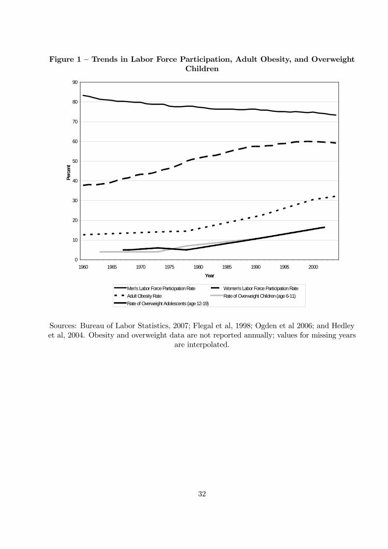
Figure 1 �Trends in Labor Force Participation, Adult Obesity, and OverweightChildren

0

10

20

30

40

50

60

70

80

90

1960 1965 1970 1975 1980 1985 1990 1995 2000

Year

Perc

ent

Men's Labor Force Participation Rate Women's Labor Force Participation RateAdult Obesity Rate Rate of Overweight Children (age 6­11)Rate of Overweight Adolescents (age 12­19)

Sources: Bureau of Labor Statistics, 2007; Flegal et al, 1998; Ogden et al 2006; and Hedleyet al, 2004. Obesity and overweight data are not reported annually; values for missing years

are interpolated.

32

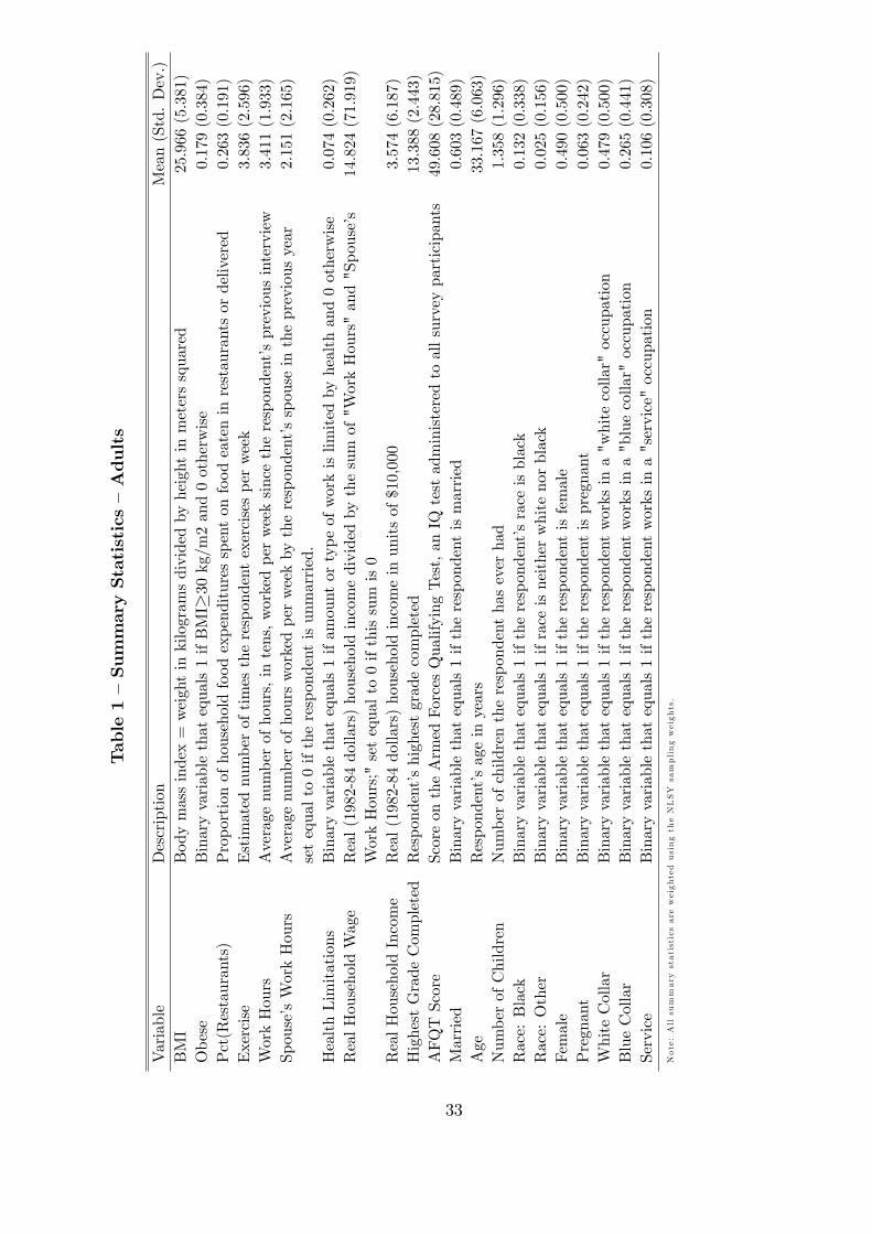
Table1�SummaryStatistics�Adults

Variable

Description

Mean(Std.Dev.)

BMI

Bodymassindex=weightinkilogramsdividedbyheightinmeterssquared

25.966(5.381)

Obese

Binaryvariablethatequals1ifBMI�30kg/m2and0otherwise

0.179(0.384)

Pct(Restaurants)

Proportionofhouseholdfoodexpendituresspentonfoodeateninrestaurantsordelivered

0.263(0.191)

Exercise

Estimatednumberoftimestherespondentexercisesperweek

3.836(2.596)

WorkHours

Averagenumberofhours,intens,workedperweeksincetherespondent�spreviousinterview

3.411(1.933)

Spouse�sWorkHours

Averagenumberofhoursworkedperweekbytherespondent�sspouseinthepreviousyear

2.151(2.165)

setequalto0iftherespondentisunmarried.

HealthLimitations

Binaryvariablethatequals1ifamountortypeofworkislimitedbyhealthand0otherwise

0.074(0.262)

RealHouseholdWage

Real(1982-84dollars)householdincomedividedbythesumof"WorkHours"and"Spouse�s

14.824(71.919)

WorkHours;"setequalto0ifthissumis0

RealHouseholdIncome

Real(1982-84dollars)householdincomeinunitsof$10,000

3.574(6.187)

HighestGradeCompleted

Respondent�shighestgradecompleted

13.388(2.443)

AFQTScore

ScoreontheArmedForcesQualifyingTest,anIQtestadministeredtoallsurveyparticipants

49.608(28.815)

Married

Binaryvariablethatequals1iftherespondentismarried

0.603(0.489)

Age

Respondent�sageinyears

33.167(6.063)

NumberofChildren

Numberofchildrentherespondenthaseverhad

1.358(1.296)

Race:Black

Binaryvariablethatequals1iftherespondent�sraceisblack

0.132(0.338)

Race:Other

Binaryvariablethatequals1ifraceisneitherwhitenorblack

0.025(0.156)

Female

Binaryvariablethatequals1iftherespondentisfemale

0.490(0.500)

Pregnant

Binaryvariablethatequals1iftherespondentispregnant

0.063(0.242)

WhiteCollar

Binaryvariablethatequals1iftherespondentworksina"whitecollar"occupation

0.479(0.500)

BlueCollar

Binaryvariablethatequals1iftherespondentworksina"bluecollar"occupation

0.265(0.441)

Service

Binaryvariablethatequals1iftherespondentworksina"service"occupation

0.106(0.308)

Note:Allsummary

statisticsareweightedusingtheNLSYsamplingweights.

33

Table2�SummaryStatistics�Children

Variable

Description

Mean(Std.Dev.)

Overweight

Binaryvariablethatequals1ifthechildisclassi�edas"overweight"and0otherwise

0.147(0.354)

Child�sAge

Child�sageinyears

9.740(4.115)

Mother�sAge

Mother�sageinyears

35.325(5.322)

NumberofChildren

Numberofchildrenunderage18livinginthehouseholdofthemother

2.423(1.154)

Child�sRace:Black

Binaryvariablethatequals1ifthechild�sraceisblackand0otherwise

0.150(0.357)

Child�sRace:Hispanic

Binaryvariablethatequals1ifthechild�sraceisHispanicand0otherwise

0.070(0.255)

Child:Female

Binaryvariablethatequals1ifthechildisfemaleand0otherwise

0.487(0.500)

OrderofBirth

Respondent�sorderofbirthtomother;1indicatesmother�s�rstchild,etc.

1.864(1.007)

MotherisOverweightorObese

Binaryvariableequalto1ifthechild�smotherisoverweightofobese

0.476(0.499)

MotherisObese

Binaryvariableequalto1ifthechild�smotherisobese

0.214(0.410)

Note:Allsummary

statisticsareweightedusingtheNLSYsamplingweights.Othervariablesinthechildren�sregressionsrepresentthemother�svaluesofthevariablesintable1.

34

Table3�E¤ectofExplanatoryVariableson

Adults�BMI/P(Obese)

BMI

Obese

(1)

(2)

(3)

(1)

(2)

(3)

WorkHours(unitsof10)

0:061

(0:015)���

0:178

(0:072) ��

0:193

(0:106)�

0:007

(0:001)���

0:012

(0:005)��

0:020

(0:011)�

Unmarried*WorkHours

��

�0:131

(0:137)

��

�0:012

(0:014)

Spouse�sWorkHours(unitsof10)

�0:014

(0:018)

0:108

(0:059)�

0:041

(0:113)

�0:006

(0:002)���

�0:0002

(0:006)

0:004

(0:011)

WorkHours*Spouse�sWorkHours

��

0:021

(0:027)

��

�0:001

(0:003)

HealthLimitations

1:111

(0:124)���

1:169

(0:416)���

1:158

(0:415)���

0:061

(0:012)���

0:068

(0:041)

0:067

(0:041)

RealHouseholdWage

�0:0003

(0:0003)

�0:0003

(0:0004)

�0:0003

(0:0004)

�0:00006

(0:00003)�

�0:0006

(0:0004)

�0:0006

(0:0004)

HighestGradeCompleted

�0:116

(0:022)���

0:102

(0:116)

0:111

(0:116)

�0:014

(0:002)���

0:001

(0:010)

0:001

(0:010)

AFQTScore

�0:008

(0:002)���

��

�0:0002

(0:0002)��

��

Married

0:436

(0:074)���

0:348

(0:217)

�0:094

(0:552)

0:031

(0:007)���

0:054

(0:024)��

0:012

(0:047)

Age

0:043

(0:017)��

�0:064

(0:054)

�0:064

(0:054)

0:004

(0:001)��

�0:004

(0:006)

�0:004

(0:006)

NumberofChildren

�0:160

(0:028)���

�0:307

(0:097)���

�0:308

(0:096)���

�0:003

(0:003)

�0:009

(0:010)

�0:009

(0:011)

Race:Black

1:488

(0:155)���

��

0:085

(0:010)���

��

Race:Other

0:531

(0:306)�

��

0:030

(0:020)

��

Female

�1:160

(0:101)���

��

0:014

(0:007)�

��

Pregnant

0:505

(0:037)���

0:583

(0:105)���

0:569

(0:105)���

0:019

(0:004)���

0:022

(0:009)��

0:021

(0:009)��

NumberofObservations

85,298

24,758

24,758

85,298

24,758

24,758

R2

0.092

0.009

0.009

0.053

0.003

0.003

Notes:(1)Randome¤ects,(2)Longdi¤erences,(3)Longdi¤erenceswithinteractionterms,***representsstatisticallysigni�cantatthe1%level;**5%level;

*10%level.All

regressionsincludeaseriesofbinary

variablesthatrepresentinterviewyears;they

aredi¤erencedin(2)and(3).Heteroskedasticity-robust

standard

errorsareinparentheses.Errorsin(2)and(3)areclustered

byindividual.ObservationsareweightedusingtheNLSYsamplingweights;weightsin(2)

and(3)aretheaveragefromthetwoperiodsusedto

createthedi¤erences.

35

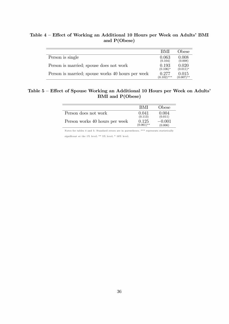
Table 4 �E¤ect of Working an Additional 10 Hours per Week on Adults�BMIand P(Obese)

BMI ObesePerson is single 0:063

(0:104)0:008(0:008)

Person is married; spouse does not work 0:193(0:106)�

0:020(0:011)�

Person is married; spouse works 40 hours per week 0:277(0:102)���

0:015(0:007)��

Table 5 �E¤ect of Spouse Working an Additional 10 Hours per Week on Adults�BMI and P(Obese)

BMI ObesePerson does not work 0:041

(0:113)0:004(0:011)

Person works 40 hours per week 0:125(0:061)��

�0:001(0:006)

Notes for tab les 4 and 5: Standard errors are in parentheses. *** represents statistica lly

sign i�cant at the 1% level; ** 5% level; * 10% level.

36

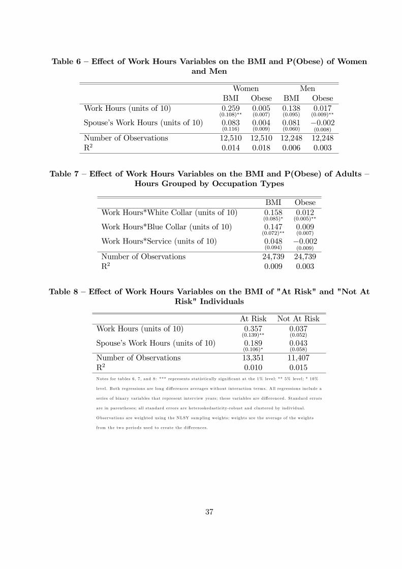
Table 6 �E¤ect of Work Hours Variables on the BMI and P(Obese) of Womenand Men

Women MenBMI Obese BMI Obese

Work Hours (units of 10) 0:259(0:108)��

0:005(0:007)

0:138(0:095)

0:017(0:009)��

Spouse�s Work Hours (units of 10) 0:083(0:116)

0:004(0:009)

0:081(0:060)

�0:002(0:008)

Number of Observations 12,510 12,510 12,248 12,248R2 0.014 0.018 0.006 0.003

Table 7 �E¤ect of Work Hours Variables on the BMI and P(Obese) of Adults �Hours Grouped by Occupation Types

BMI ObeseWork Hours*White Collar (units of 10) 0:158

(0:085)�0:012(0:005)��

Work Hours*Blue Collar (units of 10) 0:147(0:072)��

0:009(0:007)

Work Hours*Service (units of 10) 0:048(0:094)

�0:002(0:009)

Number of Observations 24,739 24,739R2 0.009 0.003

Table 8 �E¤ect of Work Hours Variables on the BMI of "At Risk" and "Not AtRisk" Individuals

At Risk Not At RiskWork Hours (units of 10) 0:357

(0:139)��0:037(0:052)

Spouse�s Work Hours (units of 10) 0:189(0:106)�

0:043(0:058)

Number of Observations 13,351 11,407R2 0.010 0.015Notes for tab les 6 , 7 , and 8: *** represents statistica lly sign i�cant at the 1% level; ** 5% level; * 10%

level. Both regressions are long di¤erences averages w ithout interaction term s. A ll regressions include a

series of b inary variab les that represent interv iew years; these variab les are d i¤erenced . Standard errors

are in parentheses; a ll standard errors are heteroskedastic ity-robust and clustered by ind iv idual.

Observations are weighted using the NLSY sampling weights; weights are the average of the weights

from the two p eriods used to create the d i¤erences.

37

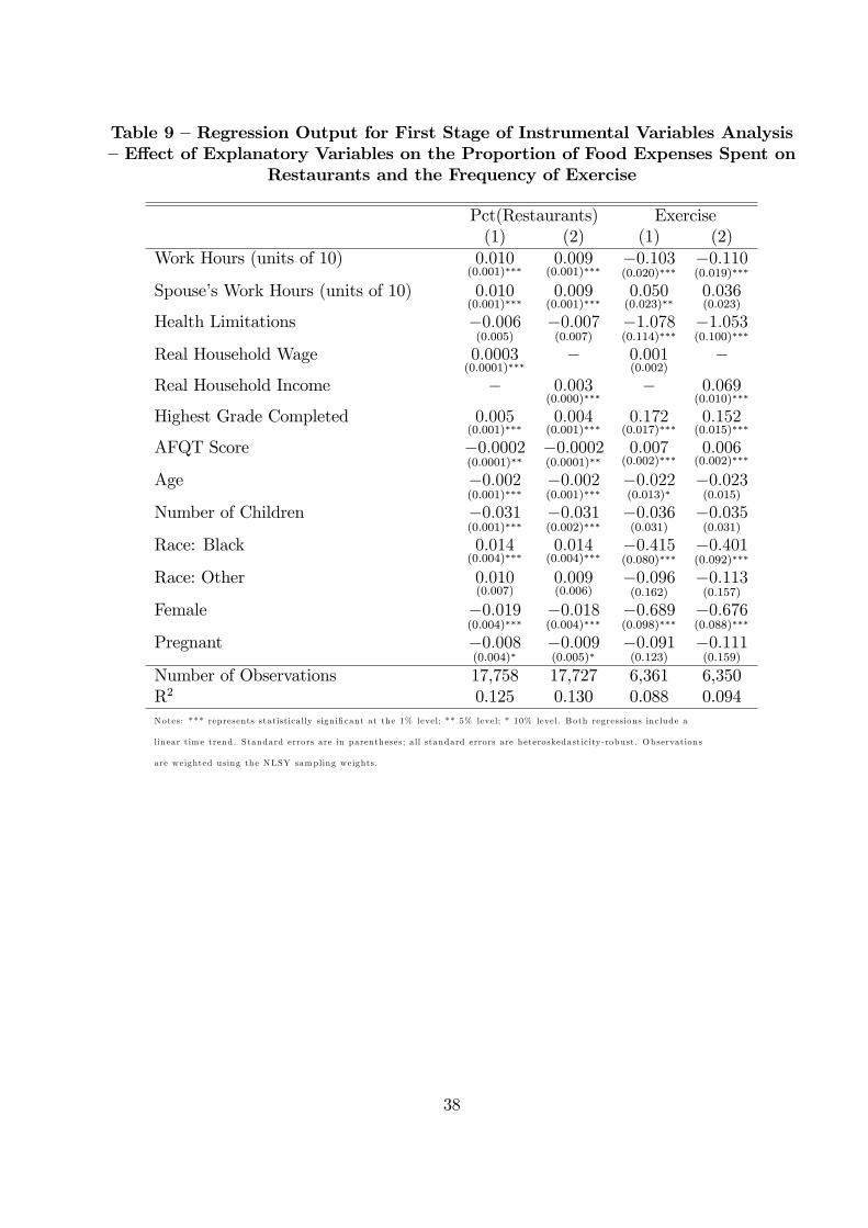
Table 9 �Regression Output for First Stage of Instrumental Variables Analysis�E¤ect of Explanatory Variables on the Proportion of Food Expenses Spent on

Restaurants and the Frequency of Exercise

Pct(Restaurants) Exercise(1) (2) (1) (2)

Work Hours (units of 10) 0:010(0:001)���

0:009(0:001)���

�0:103(0:020)���

�0:110(0:019)���

Spouse�s Work Hours (units of 10) 0:010(0:001)���

0:009(0:001)���

0:050(0:023)��

0:036(0:023)

Health Limitations �0:006(0:005)

�0:007(0:007)

�1:078(0:114)���

�1:053(0:100)���

Real Household Wage 0:0003(0:0001)���

� 0:001(0:002)

�

Real Household Income � 0:003(0:000)���

� 0:069(0:010)���

Highest Grade Completed 0:005(0:001)���

0:004(0:001)���

0:172(0:017)���

0:152(0:015)���

AFQT Score �0:0002(0:0001)��

�0:0002(0:0001)��

0:007(0:002)���

0:006(0:002)���

Age �0:002(0:001)���

�0:002(0:001)���

�0:022(0:013)�

�0:023(0:015)

Number of Children �0:031(0:001)���

�0:031(0:002)���

�0:036(0:031)

�0:035(0:031)

Race: Black 0:014(0:004)���

0:014(0:004)���

�0:415(0:080)���

�0:401(0:092)���

Race: Other 0:010(0:007)

0:009(0:006)

�0:096(0:162)

�0:113(0:157)

Female �0:019(0:004)���

�0:018(0:004)���

�0:689(0:098)���

�0:676(0:088)���

Pregnant �0:008(0:004)�

�0:009(0:005)�

�0:091(0:123)

�0:111(0:159)

Number of Observations 17,758 17,727 6,361 6,350R2 0.125 0.130 0.088 0.094Notes: *** represents statistica lly sign i�cant at the 1% level; ** 5% level; * 10% level. Both regressions include a

linear tim e trend . Standard errors are in parentheses; a ll standard errors are heteroskedastic ity-robust. Observations

are weighted using the NLSY sampling weights.

38

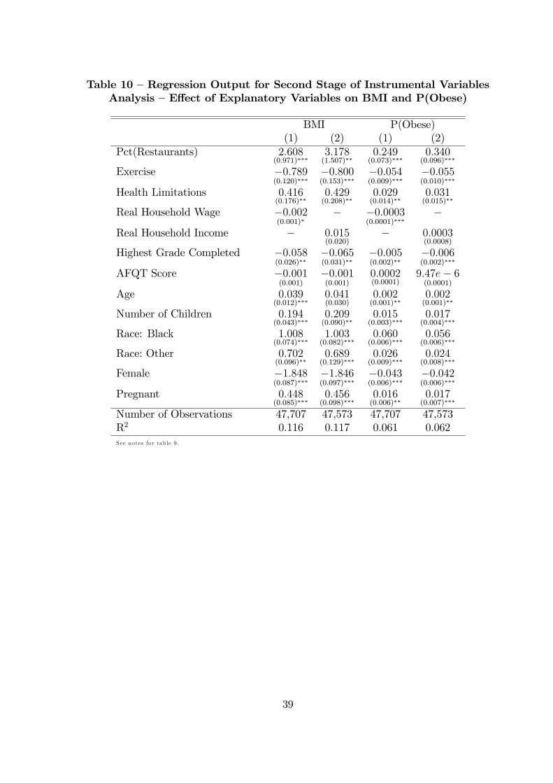
Table 10 �Regression Output for Second Stage of Instrumental VariablesAnalysis �E¤ect of Explanatory Variables on BMI and P(Obese)

BMI P(Obese)(1) (2) (1) (2)

Pct(Restaurants) 2:608(0:971)���

3:178(1:507)��

0:249(0:073)���

0:340(0:096)���

Exercise �0:789(0:120)���

�0:800(0:153)���

�0:054(0:009)���

�0:055(0:010)���

Health Limitations 0:416(0:176)��

0:429(0:208)��

0:029(0:014)��

0:031(0:015)��

Real Household Wage �0:002(0:001)�

� �0:0003(0:0001)���

�

Real Household Income � 0:015(0:020)

� 0:0003(0:0008)

Highest Grade Completed �0:058(0:026)��

�0:065(0:031)��

�0:005(0:002)��

�0:006(0:002)���

AFQT Score �0:001(0:001)

�0:001(0:001)

0:0002(0:0001)

9:47e� 6(0:0001)

Age 0:039(0:012)���

0:041(0:030)

0:002(0:001)��

0:002(0:001)��

Number of Children 0:194(0:043)���

0:209(0:090)��

0:015(0:003)���

0:017(0:004)���

Race: Black 1:008(0:074)���

1:003(0:082)���

0:060(0:006)���

0:056(0:006)���

Race: Other 0:702(0:096)��

0:689(0:129)���

0:026(0:009)���

0:024(0:008)���

Female �1:848(0:087)���

�1:846(0:097)���

�0:043(0:006)���

�0:042(0:006)���

Pregnant 0:448(0:085)���

0:456(0:098)���

0:016(0:006)��

0:017(0:007)���

Number of Observations 47,707 47,573 47,707 47,573R2 0.116 0.117 0.061 0.062See notes for tab le 9 .

39

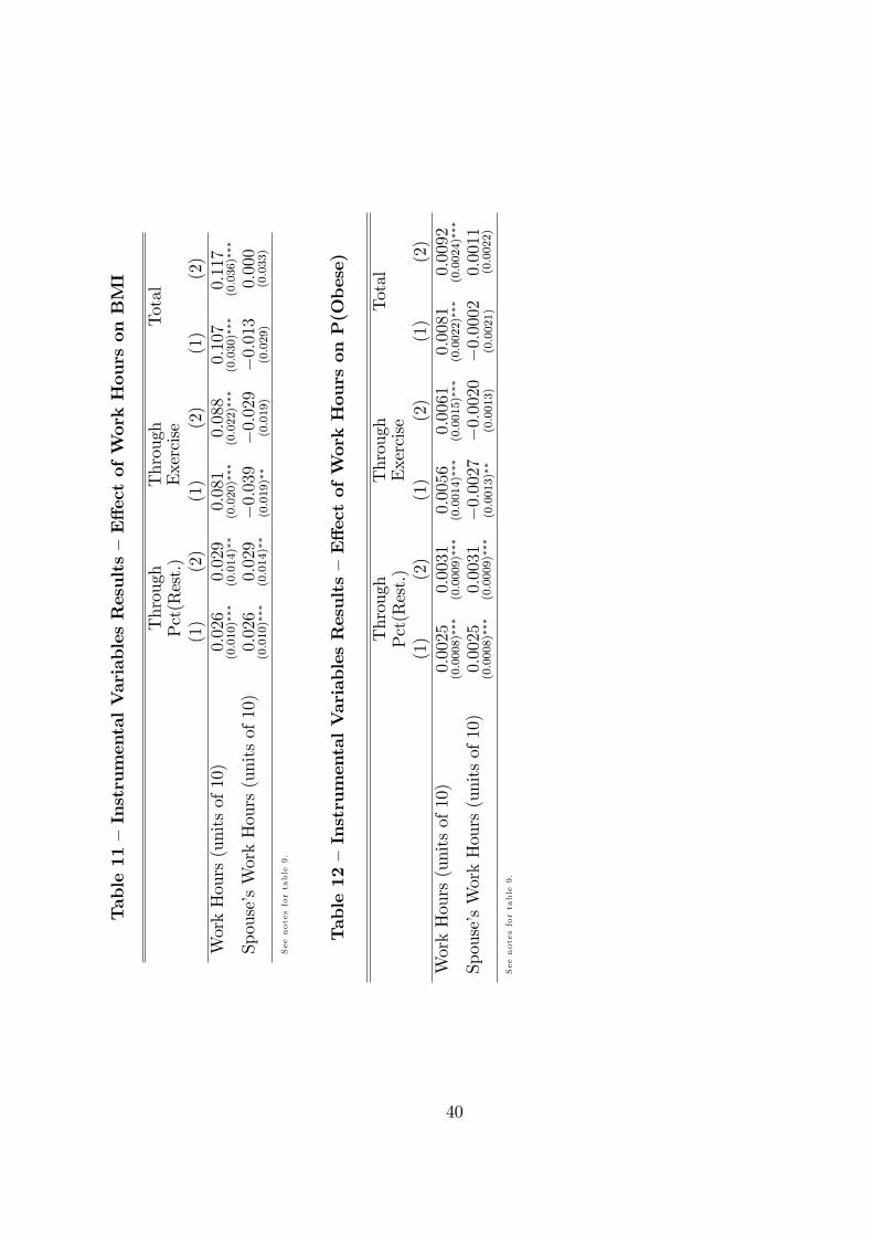
Table11�InstrumentalVariablesResults�E¤ectofWorkHourson

BMI

Through

Pct(Rest.)

Through

Exercise

Total

(1)

(2)

(1)

(2)

(1)

(2)

WorkHours(unitsof10)

0:026

(0:010)���

0:029

(0:014)��

0:081

(0:020)���

0:088

(0:022)���

0:107

(0:030)���

0:117

(0:036)���

Spouse�sWorkHours(unitsof10)

0:026

(0:010)���

0:029

(0:014)���0:039

(0:019)��

�0:029

(0:019)

�0:013

(0:029)

0:000

(0:033)

See

notesfortable9.

Table12�InstrumentalVariablesResults�E¤ectofWorkHourson

P(Obese)

Through

Pct(Rest.)

Through

Exercise

Total

(1)

(2)

(1)

(2)

(1)

(2)

WorkHours(unitsof10)

0:0025

(0:0008)���

0:0031

(0:0009)���

0:0056

(0:0014)���

0:0061

(0:0015)���

0:0081

(0:0022)���

0:0092

(0:0024)���

Spouse�sWorkHours(unitsof10)

0:0025

(0:0008)���

0:0031

(0:0009)���

�0:0027

(0:0013)��

�0:0020

(0:0013)

�0:0002

(0:0021)

0:0011

(0:0022)

See

notesfortable9.

40

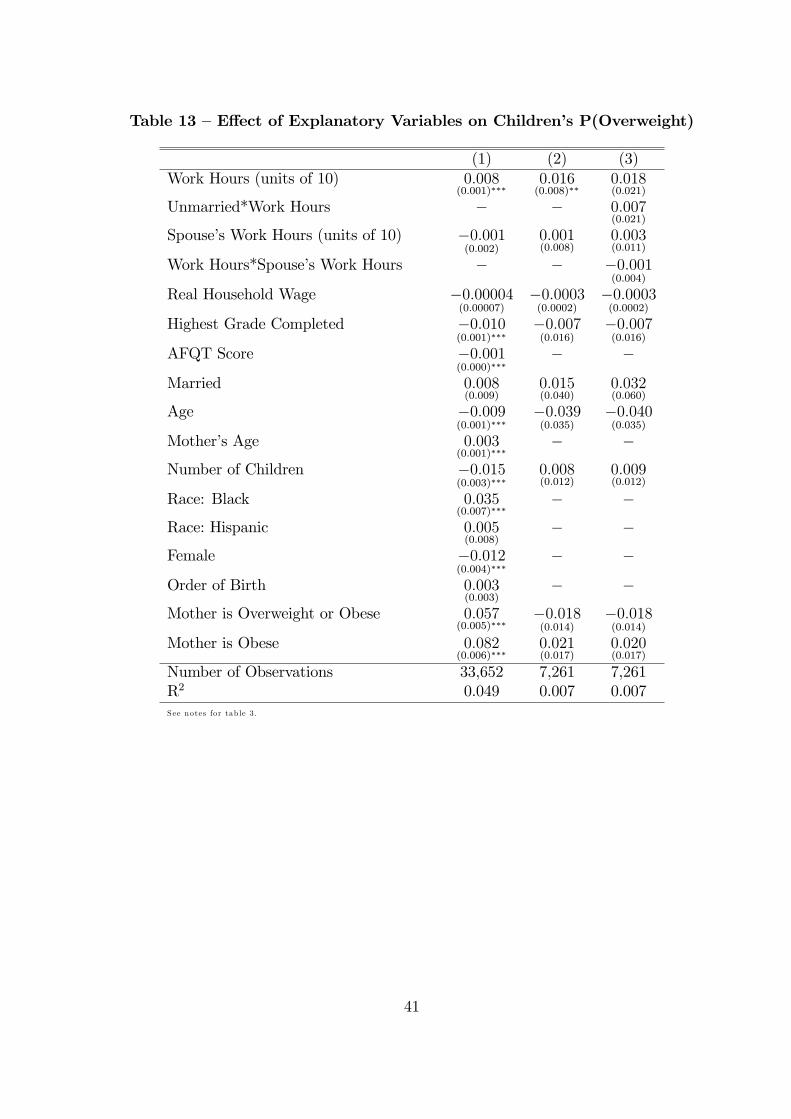
Table 13 �E¤ect of Explanatory Variables on Children�s P(Overweight)

(1) (2) (3)Work Hours (units of 10) 0:008

(0:001)���0:016(0:008)��

0:018(0:021)

Unmarried*Work Hours � � 0:007(0:021)

Spouse�s Work Hours (units of 10) �0:001(0:002)

0:001(0:008)

0:003(0:011)

Work Hours*Spouse�s Work Hours � � �0:001(0:004)

Real Household Wage �0:00004(0:00007)

�0:0003(0:0002)

�0:0003(0:0002)

Highest Grade Completed �0:010(0:001)���

�0:007(0:016)

�0:007(0:016)

AFQT Score �0:001(0:000)���

� �

Married 0:008(0:009)

0:015(0:040)

0:032(0:060)

Age �0:009(0:001)���

�0:039(0:035)

�0:040(0:035)

Mother�s Age 0:003(0:001)���

� �

Number of Children �0:015(0:003)���

0:008(0:012)

0:009(0:012)

Race: Black 0:035(0:007)���

� �

Race: Hispanic 0:005(0:008)

� �

Female �0:012(0:004)���

� �

Order of Birth 0:003(0:003)

� �

Mother is Overweight or Obese 0:057(0:005)���

�0:018(0:014)

�0:018(0:014)

Mother is Obese 0:082(0:006)���

0:021(0:017)

0:020(0:017)

Number of Observations 33,652 7,261 7,261R2 0.049 0.007 0.007See notes for tab le 3 .

41

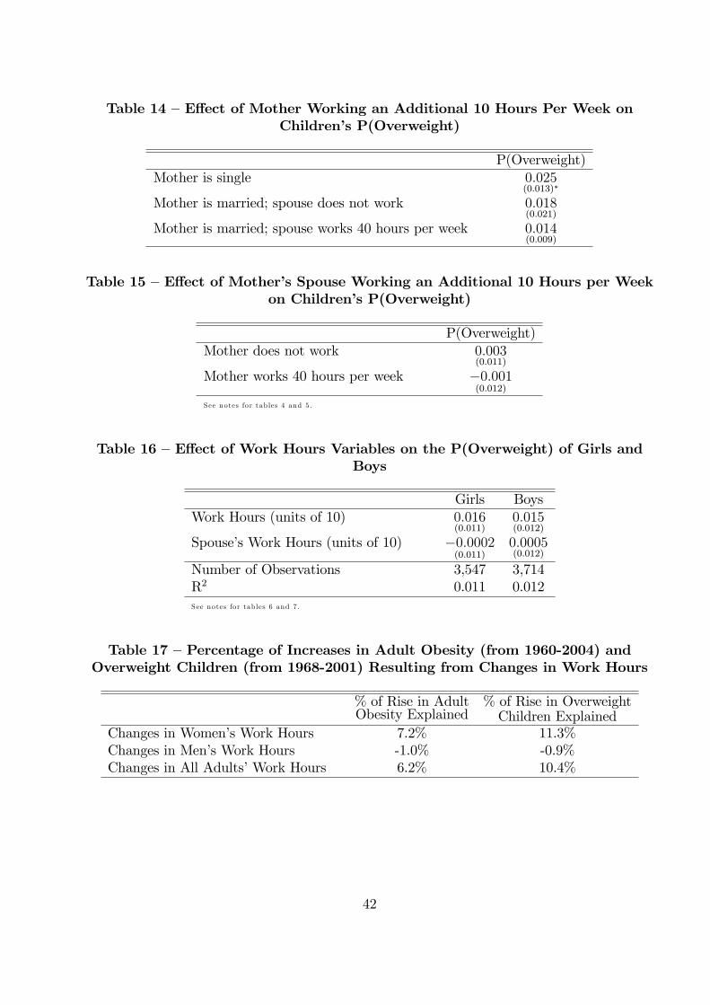
Table 14 �E¤ect of Mother Working an Additional 10 Hours Per Week onChildren�s P(Overweight)

P(Overweight)Mother is single 0:025

(0:013)�

Mother is married; spouse does not work 0:018(0:021)

Mother is married; spouse works 40 hours per week 0:014(0:009)

Table 15 �E¤ect of Mother�s Spouse Working an Additional 10 Hours per Weekon Children�s P(Overweight)

P(Overweight)Mother does not work 0:003

(0:011)

Mother works 40 hours per week �0:001(0:012)

See notes for tab les 4 and 5.

Table 16 �E¤ect of Work Hours Variables on the P(Overweight) of Girls andBoys

Girls BoysWork Hours (units of 10) 0:016

(0:011)0:015(0:012)

Spouse�s Work Hours (units of 10) �0:0002(0:011)

0:0005(0:012)

Number of Observations 3,547 3,714R2 0.011 0.012See notes for tab les 6 and 7.

Table 17 �Percentage of Increases in Adult Obesity (from 1960-2004) andOverweight Children (from 1968-2001) Resulting from Changes in Work Hours

% of Rise in AdultObesity Explained

% of Rise in OverweightChildren Explained

Changes in Women�s Work Hours 7.2% 11.3%Changes in Men�s Work Hours -1.0% -0.9%Changes in All Adults�Work Hours 6.2% 10.4%

42