Embed Size (px)
Citation preview
Munich Personal RePEc Archive
Does urbanization cause increasing
energy demand in Pakistan? Empirical
evidence from STIRPAT model
Shahbaz, Muhammad and Chaudhary, A. R. and Ozturk,
Ilhan
COMSATS Institute of Information Technology, Pakistan, National
College of Business Administration Economics, Pakistan,
University, Turkey
2 March 2016
Online at https://mpra.ub.uni-muenchen.de/70313/
MPRA Paper No. 70313, posted 25 Apr 2016 14:11 UTC
1
Does urbanization cause increasing energy demand in Pakistan? Empirical evidence
from STIRPAT model
Muhammad Shahbaz
Energy Research Center,
COMSATS Institute of Information Technology,
Defense Road, Off Raiwind Road, Lahore, Pakistan.
Email: [email protected]
A. R. Chaudhary
School of Social Sciences,
National College of Business Administration & Economics, 40/E-1, Gulberg III, Lahore-54660, Pakistan.
Email: [email protected]
Ilhan Ozturk Corresponding author
Faculty of Economics and Administrative Sciences, Cag University, 33800, Mersin, Turkey.
Email: [email protected]
Abstract: This paper reinvestigates the relationship between urbanization and energy
consumption in case of Pakistan for the period of 1972Q1-2011Q4 by employing the
STIRPAT (Stochastic Impact by Regression on Population, Affluence and Technology)
model. We have employed the ARDL bounds testing approach to cointegration in the
presence of structural breaks stemming in the series to count for these missing elements in
other studies. Finally, the VECM Granger causality approach has been applied to examine the
causal relationship between the variables. Our results show that urbanization adds in energy
consumption. Affluence (economic growth) increases energy demand. Technology has
positive impact on energy consumption. An increase in transportation is positively linked
with energy consumption. The causality analysis indicates the unidirectional causality
running from urbanization to energy consumption.
Keywords: Urbanization, Energy Demand, STIRPAT, Pakistan
2
1. Introduction
Economic theory postulates that urbanization is caused by economic growth and social
modernization [1, 2]. Poumanyvong and Kaneko [2] argued that urbanization means a shift of
the rural labor force from agricultural sector to industrial sector which is mostly situated in
urban areas. This structural transformation of rural areas into urban hubs affects energy
consumption significantly through various channels. For example, urbanization increases
energy consumption by raising the demand for housing, food, public utilities, land use,
transportation in urban areas, use of more electric appliances, the rise in demand of road use,
globalization,… etc. In recent decades, urbanization has been growing rapidly. The world
urban population was 1.52 billion in 1974-75 which steadily increased to 3.29 billion in 2006-
07 ([3]) that is projected to double in 2050. This rapid increase in urbanization will generate
more pressure on existing urban infrastructure e.g. housing, health, education, power,
transportation, and other public utilities. Urban dwellers consume higher quantities of
resources and add pressure to the flimsy ecosystem. International Energy Agency [4] reports
that big city dwellers accounted for 67.77 per cent of world energy use. This implies that the
continuous increase in urbanization will have significant impact on energy consumption.
The estimated population of Pakistan was about 62 million in 1971 with a density of 81/km
and the urban population was 25.1%. Between 1971 and 2004, population increased to 148
million, which raised urban population to 34.6% while population density was of 187/km.
Pakistan was listed among the most urbanized nations in the South Asia [5]. The urban
population rose to 36.38% [6]. In Pakistan, urban population has increased from 25.3185 per
cent as a share of total population in 1971-72 to 37.2354 per cent as a share of total
population in 2010-11, which is almost a 47 per cent rise in urban population growth [6]. This
increase in urbanization affected the contribution of modern sector, i.e. interaction between
industrial and services sectors. The share of modern sector had increased from PRS 13.75
million in 1971-72 to PRS 148.42 million in 2010-11 which is almost 979 per cent growth in
modern sector of Pakistan [6]. The urbanization also raises the demand for personnel as well
as public transportation. The use of transport was 2.97 per kilometer of road in 1971-72,
which has increased to 11.89 per kilometer of road in 2010-11, which is 300 per cent increase
in transportation use in Pakistan [6].
3
We find that rapid urbanization, modern sector growth and rapid transportation growth affect
energy demand in Pakistan. This motivates the researchers to conduct this piece of research
for providing guidelines to help policy making authorities in designing appropriate policy for
using urbanization as economic tool for efficient use of energy to maintain sustainable
economic development. Therefore, this paper contributes to the existing literature in four
ways: (i) Pakistan is an emerging economy and transportation sector consumes major chunk
of energy such s oil consumption. So, we employ augmented STIRPAT model to investigate
the relationship between urbanization and energy consumption by incorporating affluence,
technology and transportation as potential determinants of urbanization and energy demand.
(ii) Over the sample period of time, structural breaks occurred in urbanization, energy,
industrialization, economic growth etc. due to implementation of economic, urban and energy
policies by the government. These structural breaks may change the unit root behavior,
impact (effect) of the variables and even change the causal relationship between the variables.
In doing so, the structural break unit tests are employed to test the stationarity properties of
the variables. (iii) The cointegration relationship between the variables is examined by
applying the ARDL bounds testing accommodating structural breaks in the series. (iv) The
VECM causality approach is used to check causal relationship between urbanization and
energy demand by accommodating structural breaks occurring in the series. We find that
presence of structural breaks in the series could not affect cointegration relationship between
the variables i.e. cointegration exists. Additionally, urbanization is positively linked with
energy consumption. Affluence and technological development positively affect energy
consumption. Transportation has positive effect on energy consumption. The causality
analysis reveals that energy consumption is cause of urbanization. The feedback effect is
noted between technological development (transportation) and energy consumption.
Affluence causes energy consumption and energy consumption causes affluence.
2. Literature Review
The relationship between urbanization and energy consumption has been widely and
empirically investigated by various researchers in the existing literature. For example, Jones
[7] noted that urbanization raises energy demand because urban people are more connected to
electrical appliances as compared to rural individuals. In urban areas, there is an increase in
private transportation with an increase in income per capita which also contributes to energy
demand. Energy demand is also cause of urban density. Dhal and Erdogan [8] examined the
relationship between urban population and oil consumption. They reported that an increase in
4
urbanization is positively linked to industrialization, which increases oil consumption. Burney
[9] reported that socioeconomic determinants also affect energy consumption. He found that
urbanization raises energy demand, but varies across countries by keeping income per capita
and industrialization constant. Imai [10] found that population and urbanization has positive
impact on energy consumption but causality results exposed that urbanization is cause of
population and energy consumption.
Later on, Cole and Nuemayer [11] reported that urbanization is directly linked with energy
demand due to rise in demand for housing, transportation provides by government and other
public utilities, urban density and stimulation of economic activity in industrial and services
sectors. They found U-shaped relationship between urbanization and energy consumption and
small size households adds more in energy demand. Kalnay and Cal [12] pointed out that
urbanization raises pressure on agriculture sector to produce more food. This raises the use of
land as well as energy demand in agriculture sector. Bryant [13] opined that urbanization is
linked to industrialization, technological advancement, globalization and migration. All these
factors add in energy demand. Likewise, Shen et al. [14] unveiled that supply of resources i.e.
Cement, steel, aluminum and coal and the demand of timber, cement and steel, lead the
process of urbanization which increases industrialization and modernization and, in resulting
energy demand is increased.
Wang et al. [15] examined the impact factors of population, economic level, technology level,
urbanization level, industrialization level, service level, energy consumption structure and
foreign trade degree on the energy-related CO2 emissions in Guangdong Province, China
from 1980 to 2010 using an extended STIRPAT model. Empirical results indicate that factors
such as population, urbanization level, GDP per capita, industrialization level and service
level, can cause an increase in CO2 emissions. However, technology level, energy
consumption structure and foreign trade degree can lead to a decrease in CO2 emissions.
Mishra et al. [16] investigated the affiliation between urbanization and energy consumption
by incorporating economic growth in the energy demand function in Pacific Island nations.
They noted that urbanization involves structural changes throughout the economy and has
important implications for energy consumption. Urbanization leads to substantial
concentration of population in generating economic activities; and thus increases demand for
energy. Lui [17] assessed the relationship between population growth, urbanization and
energy consumption by applying the ARDL bounds testing approach and factor
5
decomposition model in case of Chinese economy. He found that the cointegration for the
long run rapport is present among the variables. The causality analysis revealed that
population and economic growth have neutral impact on energy consumption, but total
energy consumption is cause of urbanization. Zhao-hui [18] reinvestigated the relationship
between different stages of urbanization (tortuous development, early stage and mid-stage)
and energy consumption. The results showed cointegration between the variables and energy
demand Granger causes both industrial development and urbanization.
Similarly, Poumanyvong and Kaneko [2] looked into the relationship between urbanization
and energy consumption by incorporating other potential variables such as economic growth,
industrial development and population growth in the energy demand function. Their empirical
evidence found that urbanization, economic growth, population and industrialization add in
energy demand but technical efficiency lowers it. Furthermore, they reported that in
developing economies, urbanization reduces energy demand due to switch off from
traditional and inefficient energy fuels to modern and efficient energy fuels. The positive
effect of urbanization on energy consumption is greater in high income countries compared to
middle income economies. Madlener and Sunk [19] examined the impact of urbanization and
urban structure on energy consumption using data of 100 developed and developing
economies. They found that urbanization affects energy demand via changes in urban
structure. Their results confirmed that urbanization is cause of economic development and
increase in income levels changes the consumer necessities which in turn affect energy
consumption. Shahbaz and Lean [20] analyzed the relationship between urbanization and
energy consumption by incorporating financial development and industrialization in energy
demand function. Their empirical evidence showed that financial development,
industrialization and urbanization have positive impact on energy consumption in Tunisia.
Likewise, urbanization and financial development lead industrialization, which Granger
causes energy demand. Similarly, Islam et al. [21] also found that population is positively
linked with energy demand, but the bidirectional causal relationship is found between
population and energy consumption in case of Malaysia.
Ma and Du [22] reinvestigated the relationship between urbanization, industrialization,
energy prices and energy consumption using data of Chinese economy. They found that
industrialization leads urbanization and urbanization has positive impact on energy demand
due to an increase in urban density. Additionally, impact of tertiary industrial value added is
6
negative on energy use due to use of advance technology and Chinese energy policy as well
as environmental regulations. Apart from that, Mickieka and Fletcher [23] tested the impact
of urbanization on coal consumption using the vector autoregressive framework and Toda and
Yamamoto [24] Granger causality approach over the period of 1971-2009. They incorporated
real GDP and electricity production as potential determinants in coal demand function. Their
empirical evidence exposed that coal consumption is cause of economic growth and the
unidirectional causality is found running from urbanization to electricity consumption as well
as coal consumption. Coal consumption does not seem to affect real GDP. Zhang and Lin
[25] analyzed the impact of urbanization on energy consumption using national, provincial
and regional data by applying the STIRPAT model. Their empirical evidence opined that
urbanization has positive impact on energy consumption but varies across regions.
Urbanization also lowers energy demand in West, Central and Eastern regions of China due
to use of energy efficient technology.
Poumanyvong et al. [26] reinvestigated the impact of urbanization on national transport and
road energy use using the data of developing, middle and high income countries. Their results
showed that urbanization raises more demand for transportation and hence energy in high
income countries comparatively in low income countries. Surprisingly, the impact of
urbanization on national transport and hence on energy consumption is positive but less in
middle income countries as compared to low income countries. Sadorsky [27] collected the
data of 75 developing countries, including Pakistan to examine the impact of urbanization and
industrialization on energy intensity by applying the mean group estimator (MGE). He found
that income effect has negative impact on energy intensity i.e. -0.45%-0.35%. This suggests
that rise in income leads to employ advance and energy efficient technology for enhancing
domestic production which reduces energy consumption. Furthermore, industrialization
increases, i.e. 0.07%-0.12% energy intensity and impact of urbanization on energy intensity
varies in various regions. Solarin and Shahbaz [28] applied the trivariate model to assess the
causality between energy consumption (electricity consumption) using annual frequency data
for Angola economy. They investigated the long run relationship by applying the ARDL
bounds testing and the VECM Granger causality is applied for causality between the
variables. Their empirical exercise exposed that electricity consumption and urbanization
promote economic growth. The causality results revealed that the relationship between
electricity consumption and urbanization is bidirectional.
7
In a comparative study, Pachauri and Jiang [29] noted that rural individuals consume more
energy due to the heavy dependence on inefficient energy fuels and these energy fuels meet
85% of rural energy demand in China and India. In particular, O'Neill et al. [30] applied
iPETS (integrated-Population-Economy-Technology-Science) model to reassess the impact of
urbanization on energy use in India and China. Their study noted that urbanization has impact
on energy use but less than proportional in both countries due to the fast rate of urbanization
which provides labor supply to enhance domestic production. Moreover, rural-urban disparity
between China and India also affects the household energy consumption. The non-linear
relationship between urbanization and energy consumption (energy demand) is also
investigated. For example, Duan et al. [31] used the data of 45 countries to assess the impact
of urbanization on energy consumption by applying the ECUGA (Energy Consumption Unit
Geometric Average) method. They found inverted U-shaped relationship between
urbanization and energy consumption. Likewise, they noted that energy intensity increases if
urbanization reaches to 40% to 50% and it starts to decline by 50% to 80% urbanization.
Jiang and Lin [32] asserted that China is shifting from low-income group to middle income-
group with faster economic growth which is supported by rapid industrialization and
urbanization. They documented that the relationship between urbanization and energy
intensity is inverted-U shaped. The theory of inverted U-shaped relationship reveals that
during the process of development, industrialization follows urbanization, energy demand is
inflexible and grows quickly due to rapid industrialization. This implies that energy
consumption (intensity) reaches to its peak during the stage of development and starts to
decline, once urbanization and industrialization are completed. Zhang and Qin (2013)
criticized the findings reported by Jiang and Lin [32] and noted that the empirical model used
by Zhang and Qin [33] has variable specification problems. Xia and Hu [34] exposed that
urbanization tends to increase the migration of labor from rural areas to urban sector due to
industrialization in China. This transformation of population has significant impact on energy
consumption. Apergis and Tang [35] used the multivariate model to test the causal
relationship between energy consumption and urbanization by including income and labor
force in the energy demand function. They applied the Toda-Yamamoto-Dolado-Luutkepohl
(TYDL) causality approach developed by Toda and Yamamoto [24] and, Dolado and
Luutkepohl [36] using the data of 85 high, middle and low income countries. Overall, their
empirical evidence revealed that energy consumption and urbanization are independent i.e.
neutral effect while energy consumption Granger causes economic growth. Brant [13] probed
the nexus between energy consumption, economic growth and urbanization using
8
heterogeneous panel data of high, middle and low income countries. The results of Pedroni
[37] reported the existence of cointegration between the variables. Urbanization leads energy
demand. The link between urbanization and energy consumption shows the phenomenon of
ladder effect. Liu and Xie [38] applied the threshold vector error correction model (TVECM)
to examine the relationship between urbanization and energy intensity in the case of China.
They noted that urbanization leads energy consumption quickly before the threshold point,
i.e. inverted U-shaped relationship between urbanization and energy consumption. The
causality analysis exposed that urbanization causes energy consumption.
Recently, Wang [39] examined the impact urbanization on residential energy consumption
and energy production in case of China. The results indicated that urbanization leads
residential energy demand. Urbanization stimulates industrialization, which enhances
economic growth and resulting energy demand is increased. Liddle and Lung [40] used data
of 105 countries to examine the direction of causality between urbanization and electricity
consumption by applying the panel Granger causality test. They found that unidirectional
causality is found running electricity consumption to urbanization. Shahbaz et al. [41] found
that Malaysian energy consumption is positively affected by Malaysian urbanization.
In case of Pakistan, Alam et al. [42] examined the impact of population growth and
urbanization on energy consumption and economic growth by applying simultaneous
equation method. They reported that long run relationship between economic growth,
population growth, urbanization and energy consumption exists. Moreover, population
growth and urbanization has positive impact on energy consumption. Zaman et al. [43]
investigated energy (measuring by electricity) demand function over the period of 1975-2010.
Their results indicated that population leads urbanization that is positively linked with energy
demand. The causality analysis showed that urbanization Granger causes energy
consumption. Ali and Nitivattananon [44] explored the interrelationship between land use and
energy consumption in case of Lahore applying an integrated and multi-disciplinary
approach. They unveiled that industrial and residential sectors are major drivers to raise
energy demand in Lahore city.
3. Theoretical Background and Model Construction
Economic growth leads to urbanization and social modernization is a well established fact [1,
2]. Urbanization is also called the renovation of rural population into urban population i.e.
9
conversion of rural areas into urban areas [2]. Urbanization leads to industrialization, which
affects energy consumption [6, 7]. Urbanization affects energy demand by raising demand for
housing, transportation and other public utilities supply by government, urban density [11].
Urbanization increases the road use due to industrial activities [45], pressurizes agriculture
sector to produce more food both for rural as well as urban population [12], increases
commercialization [46], changes urban structure [19], stimulates financial development which
leads to promotion of investment activities and industrialization [20], raises the demand for
production material [47], increases migration of labor from rural areas to the urban sector [34]
and boosts economic activity [27]. These factors are also cause of urbanization and affect
energy demand. But, transportation variable has been discussed theoretically in existing
literature but never empirically included in IPAT (Integrated Population, Affluence and
Technology) model. We have included transportation variable to capture the impact of
transportation on energy demand in Pakistan as we know that transportation sector is a
significant contributor to energy demand.
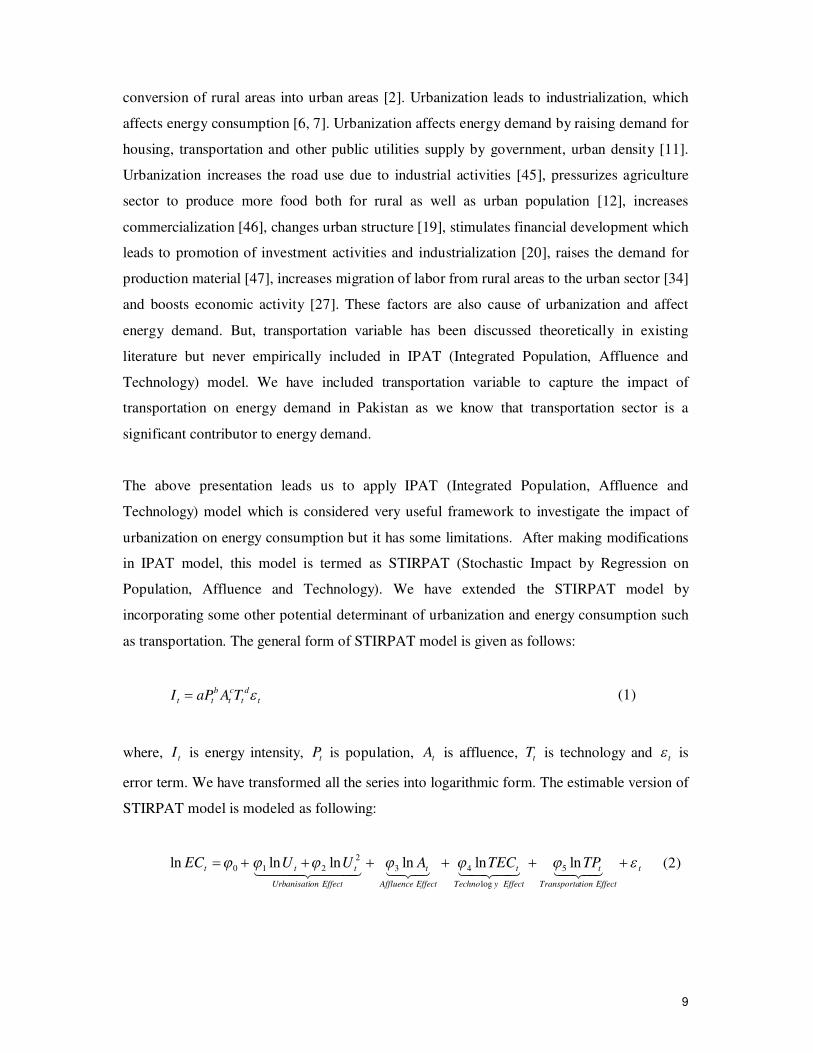
The above presentation leads us to apply IPAT (Integrated Population, Affluence and
Technology) model which is considered very useful framework to investigate the impact of
urbanization on energy consumption but it has some limitations. After making modifications
in IPAT model, this model is termed as STIRPAT (Stochastic Impact by Regression on
Population, Affluence and Technology). We have extended the STIRPAT model by
incorporating some other potential determinant of urbanization and energy consumption such
as transportation. The general form of STIRPAT model is given as follows:
t
d
t
c
t
b
tt TAaPI (1)
where, tI is energy intensity, tP
is population, tA
is affluence, tT
is technology and t
is
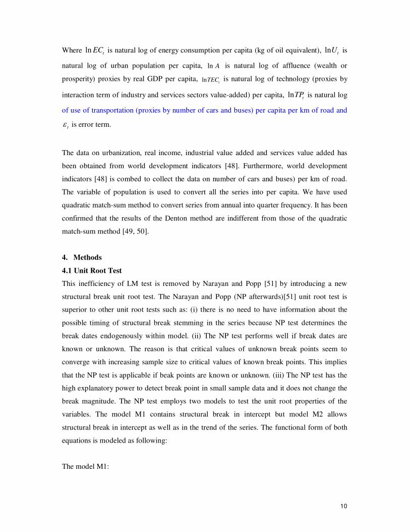
error term. We have transformed all the series into logarithmic form. The estimable version of
STIRPAT model is modeled as following:
t
EffecttionTransporta
t
EffectyTechno
t
EffectAffluence
t
EffectonUrbanisati
ttt TPTECAUUEC
lnlnlnlnlnln 5
log
43
2
210 (2)
10
Where tECln is natural log of energy consumption per capita (kg of oil equivalent), t
Uln is
natural log of urban population per capita, Aln is natural log of affluence (wealth or
prosperity) proxies by real GDP per capita, tTECln is natural log of technology (proxies by
interaction term of industry and services sectors value-added) per capita, tTPln
is natural log
of use of transportation (proxies by number of cars and buses) per capita per km of road and
t is error term.
The data on urbanization, real income, industrial value added and services value added has
been obtained from world development indicators [48]. Furthermore, world development
indicators [48] is combed to collect the data on number of cars and buses) per km of road.
The variable of population is used to convert all the series into per capita. We have used
quadratic match-sum method to convert series from annual into quarter frequency. It has been
confirmed that the results of the Denton method are indifferent from those of the quadratic
match-sum method [49, 50].
4. Methods
4.1 Unit Root Test
This inefficiency of LM test is removed by Narayan and Popp [51] by introducing a new
structural break unit root test. The Narayan and Popp (NP afterwards)[51] unit root test is
superior to other unit root tests such as: (i) there is no need to have information about the
possible timing of structural break stemming in the series because NP test determines the
break dates endogenously within model. (ii) The NP test performs well if break dates are
known or unknown. The reason is that critical values of unknown break points seem to
converge with increasing sample size to critical values of known break points. This implies
that the NP test is applicable if beak points are known or unknown. (iii) The NP test has the
high explanatory power to detect break point in small sample data and it does not change the
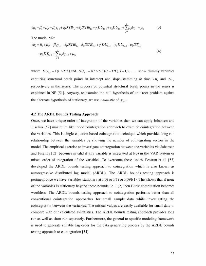
break magnitude. The NP test employs two models to test the unit root properties of the
variables. The model M1 contains structural break in intercept but model M2 allows
structural break in intercept as well as in the trend of the series. The functional form of both
equations is modeled as following:
The model M1:
11
k
j
tjtjtttttt ybDUDUTBDTBDyty1
11,221,21,22,111321 )()( (3)
The model M2:
k
j
tjtjt
ttttttt
ybDT
DTDUDUTBDTBDyty
1
21,22
1,111,221,21,22,111321)()(
(4)
where )(1, iti TBtDU and ......,2,1),()(1, iTBtTBtDU iiti show dummy variables
capturing structural break points in intercept and slope stemming at time 1
TB and 2
TB
respectively in the series. The process of potential structural break points in the series is
explained in NP [51]. Anyway, to examine the null hypothesis of unit root problem against
the alternate hypothesis of stationary, we use t-statistic of 1ty .
4.2 The ARDL Bounds Testing Approach
Once, we have unique order of integration of the variables then we can apply Johansen and
Juselius [52] maximum likelihood cointegration approach to examine cointegration between
the variables. This is single-equation based cointegration technique which provides long run
relationship between the variables by showing the number of cointegrating vectors in the
model. The empirical exercise to investigate cointegration between the variables via Johansen
and Juselius [52] becomes invalid if any variable is integrated at I(0) in the VAR system or
mixed order of integration of the variables. To overcome these issues, Pesaran et al. [53]
developed the ARDL bounds testing approach to cointegration which is also known as
autoregressive distributed lag model (ARDL). The ARDL bounds testing approach is
pertinent once we have variables stationary at I(0) or I(1) or I(0)/I(1). This shows that if none
of the variables is stationary beyond these bounds i.e. I (2) then F-test computation becomes
worthless. The ARDL bounds testing approach to cointegration performs better than all
conventional cointegration approaches for small sample data while investigating the
cointegration between the variables. The critical values are easily available for small data to
compare with our calculated F-statistics. The ARDL bounds testing approach provides long
run as well as short run separately. Furthermore, the general to specific modeling framework
is used to generate suitable lag order for the data generating process by the ARDL bounds
testing approach to cointegration [54].
12
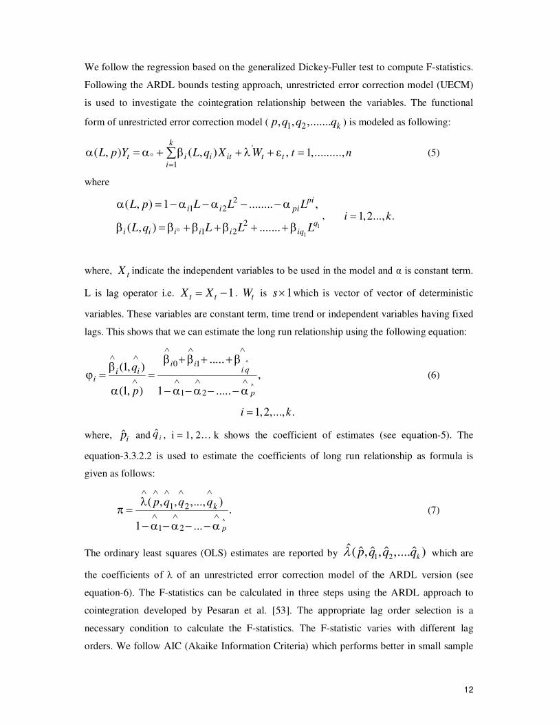
We follow the regression based on the generalized Dickey-Fuller test to compute F-statistics.
Following the ARDL bounds testing approach, unrestricted error correction model (UECM)
is used to investigate the cointegration relationship between the variables. The functional
form of unrestricted error correction model ( 1 2, , ,....... kp q q q ) is modeled as following:
'
1
( , ) ( , ) ,
k
t i i it t ti
L p Y L q X W 1,.........,t n (5)
where
1
1
21 2
21 2
( , ) 1 ........ ,
( , ) .......
pii i pi
qi i i i i iq
L p L L L
L q L L L, 1,2..., .i k
where, tX indicate the independent variables to be used in the model and α is constant term.
L is lag operator i.e. 1 t tX X . tW is 1s which is vector of vector of deterministic
variables. These variables are constant term, time trend or independent variables having fixed
lags. This shows that we can estimate the long run relationship using the following equation:
^
^
0 1
1 2
.....(1, )
,
(1, ) 1 .....
i ii qii
i
p
q
p
(6)
1,2,..., .i k
where, ˆip and iq̂ , i = 1, 2… k shows the coefficient of estimates (see equation-5). The
equation-3.3.2.2 is used to estimate the coefficients of long run relationship as formula is
given as follows:
^
1 2
1 2
( , , ,..., ).
1 ...
k
p
p q q q (7)
The ordinary least squares (OLS) estimates are reported by )ˆ....,ˆ,ˆ,ˆ(ˆ21 kqqqp which are
the coefficients of λ of an unrestricted error correction model of the ARDL version (see
equation-6). The F-statistics can be calculated in three steps using the ARDL approach to
cointegration developed by Pesaran et al. [53]. The appropriate lag order selection is a
necessary condition to calculate the F-statistics. The F-statistic varies with different lag
orders. We follow AIC (Akaike Information Criteria) which performs better in small sample
13
data as compared to SBC (Schwartz Bayesian Criteria). The performance of SBC is sensitive
with sample size. Secondly, F-statistic is calculated by using the unrestricted error correction
model (UECM) for cointegration between the series. The formulation of the autoregressive
distributive lag model is based on ( 1) kp . We see that number of variables to be used in
the model is shown by k and p reports the appropriate lag order of the variables. Lastly, we
calculate F-statistic to examine whether cointegration exists or not between the variables [55].
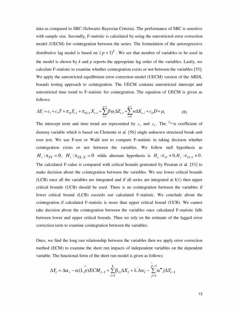
We apply the unrestricted equilibrium error correction model (UECM) version of the ARDL
bounds testing approach to cointegration. The UECM contains unrestricted intercept and
unrestricted time trend to F-statistic for cointegration. The equation of UECM is given as
follows:
iD
q
i
it
p
i
titXYXtYYTtDcXwZXYTccY
1
0
1
1
11.11 (8)
The intercept term and time trend are represented by 1
c and T
c . The Dc is coefficient of
dummy variable which is based on Clemente et al. [56] single unknown structural break unit
root test. We use F-test or Wald test to compute F-statistic in taking decision whether
cointegration exists or not between the variables. We follow null hypothesis as
: 0 YYH , .: 0 YX XH while alternate hypothesis is 0:,0: . XYXaYYa
HH .
The calculated F-value is compared with critical bounds generated by Pesaran et al. [53] to
make decision about the cointegration between the variables. We use lower critical bounds
(LCB) once all the variables are integrated and if all series are integrated at I(1) then upper
critical bounds (UCB) should be used. There is no cointegration between the variables if
lower critical bound (LCB) exceeds our calculated F-statistic. We conclude about the
cointegration if calculated F-statistic is more than upper critical bound (UCB). We cannot
take decision about the cointegration between the variables once calculated F-statistic falls
between lower and upper critical bounds. Then we rely on the estimate of the lagged error
correction term to examine cointegration between the variables.
Once, we find the long run relationship between the variables then we apply error correction
method (ECM) to examine the short run impacts of independent variables on the dependent
variable. The functional form of the short run model is given as follows:
1
'1 1
1 1
(1, )
pk
t t i t t ti j
Y p ECM X w j Y
14
1
,1 1
tqk
ij i t j ti j
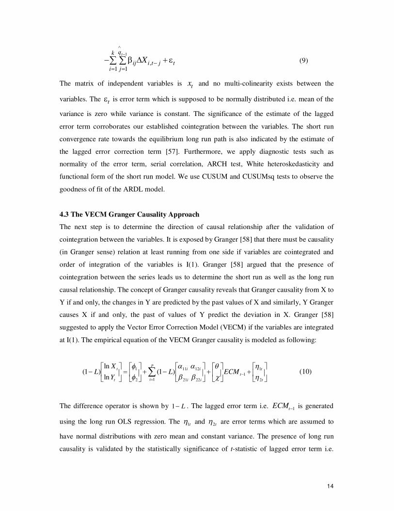
X (9)
The matrix of independent variables is tx and no multi-colinearity exists between the
variables. The t is error term which is supposed to be normally distributed i.e. mean of the
variance is zero while variance is constant. The significance of the estimate of the lagged
error term corroborates our established cointegration between the variables. The short run
convergence rate towards the equilibrium long run path is also indicated by the estimate of
the lagged error correction term [57]. Furthermore, we apply diagnostic tests such as
normality of the error term, serial correlation, ARCH test, White heteroskedasticity and
functional form of the short run model. We use CUSUM and CUSUMsq tests to observe the
goodness of fit of the ARDL model.
4.3 The VECM Granger Causality Approach
The next step is to determine the direction of causal relationship after the validation of
cointegration between the variables. It is exposed by Granger [58] that there must be causality
(in Granger sense) relation at least running from one side if variables are cointegrated and
order of integration of the variables is I(1). Granger [58] argued that the presence of
cointegration between the series leads us to determine the short run as well as the long run
causal relationship. The concept of Granger causality reveals that Granger causality from X to
Y if and only, the changes in Y are predicted by the past values of X and similarly, Y Granger
causes X if and only, the past of values of Y predict the deviation in X. Granger [58]
suggested to apply the Vector Error Correction Model (VECM) if the variables are integrated
at I(1). The empirical equation of the VECM Granger causality is modeled as following:
t
t
t
ii
iip
it
tECML
Y
XL
2
1
1
2221
1211
12
1)1(
ln
ln)1(
(10)
The difference operator is shown by L1 . The lagged error term i.e. 1tECM is generated
using the long run OLS regression. The t1 and t2 are error terms which are assumed to
have normal distributions with zero mean and constant variance. The presence of long run
causality is validated by the statistically significance of t-statistic of lagged error term i.e.
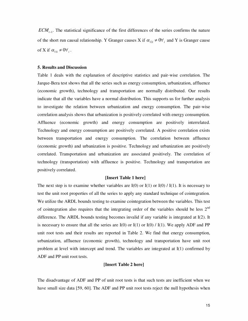
15
1tECM . The statistical significance of the first differences of the series confirms the nature
of the short run causal relationship. Y Granger causes X if ii 012 and Y is Granger cause
of X if ii 011 .
5. Results and Discussion
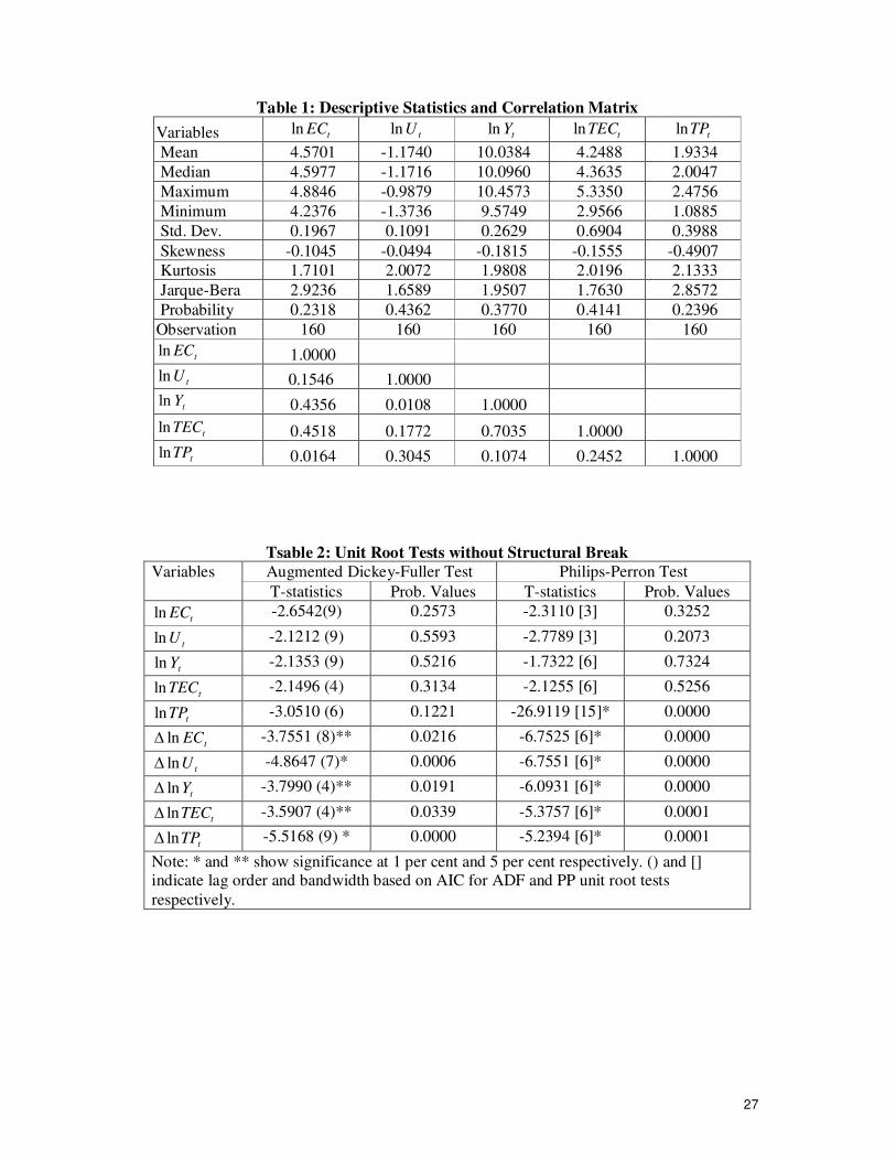
Table 1 deals with the explanation of descriptive statistics and pair-wise correlation. The
Jarque-Bera test shows that all the series such as energy consumption, urbanization, affluence
(economic growth), technology and transportation are normally distributed. Our results
indicate that all the variables have a normal distribution. This supports us for further analysis
to investigate the relation between urbanization and energy consumption. The pair-wise
correlation analysis shows that urbanization is positively correlated with energy consumption.
Affluence (economic growth) and energy consumption are positively interrelated.
Technology and energy consumption are positively correlated. A positive correlation exists
between transportation and energy consumption. The correlation between affluence
(economic growth) and urbanization is positive. Technology and urbanization are positively
correlated. Transportation and urbanization are associated positively. The correlation of
technology (transportation) with affluence is positive. Technology and transportation are
positively correlated.
[Insert Table 1 here]
The next step is to examine whether variables are I(0) or I(1) or I(0) / I(1). It is necessary to
test the unit root properties of all the series to apply any standard technique of cointegration.
We utilize the ARDL bounds testing to examine cointegration between the variables. This test
of cointegration also requires that the integrating order of the variables should be less 2nd
difference. The ARDL bounds testing becomes invalid if any variable is integrated at I(2). It
is necessary to ensure that all the series are I(0) or I(1) or I(0) / I(1). We apply ADF and PP
unit root tests and their results are reported in Table 2. We find that energy consumption,
urbanization, affluence (economic growth), technology and transportation have unit root
problem at level with intercept and trend. The variables are integrated at I(1) confirmed by
ADF and PP unit root tests.
[Insert Table 2 here]
The disadvantage of ADF and PP of unit root tests is that such tests are inefficient when we
have small size data [59, 60]. The ADF and PP unit root tests reject the null hypothesis when
16
it is false and vice versa due to their low power and mislead the unit root results.
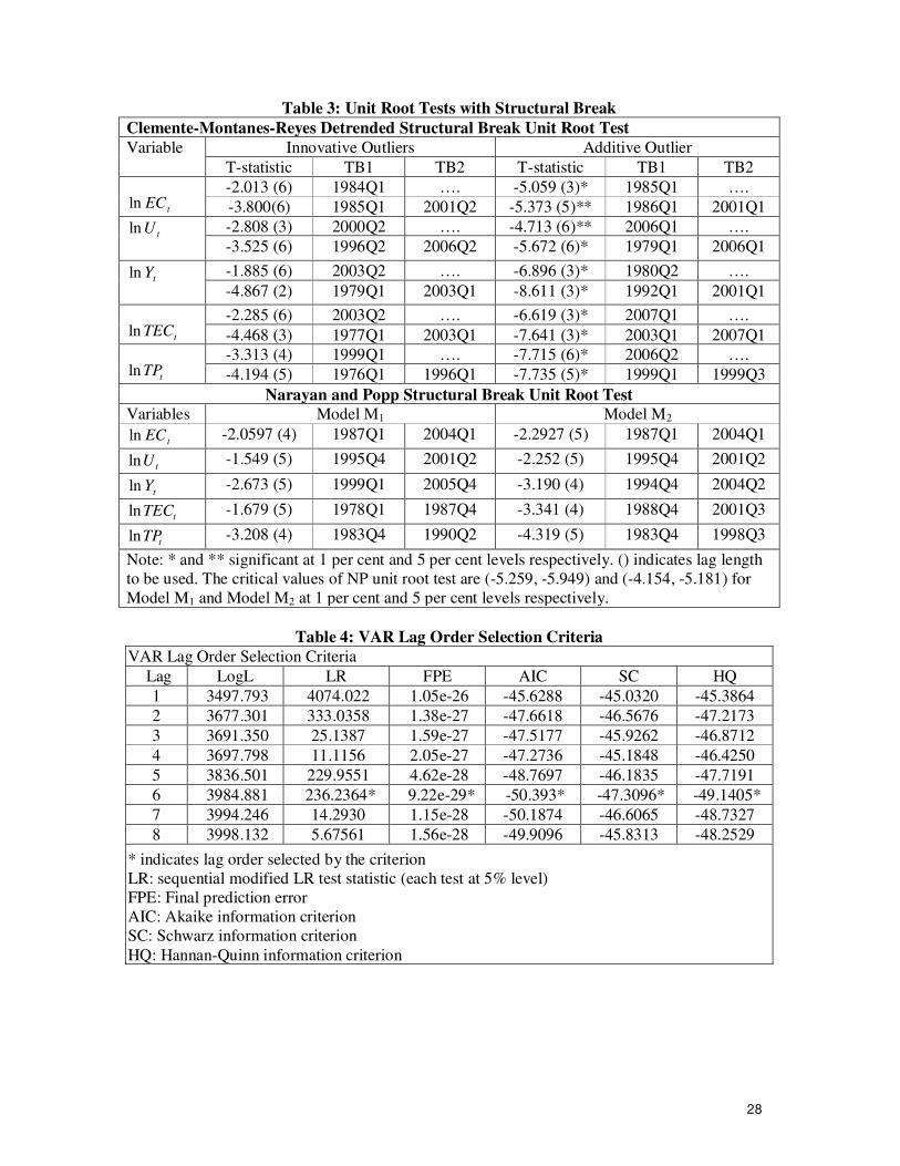
Additionally, the ADF and PP tests avoid the information of structural break stemming in the
variable which may also be cause of unit root problem in the variables. We have applied
Clemente-Montanes-Reyes [56] detrended unit root test with single and two unknown
structural breaks arising in the variables. The results reported in Table 3 reveal that all the
variables show unit root problem in the presence of structural breaks. The 1984Q1, 2000Q2,
2003Q2 and 1976Q1 are structural breaks found in the series of energy consumption,
urbanization, affluence (economic growth), technology and transportation. The structural
break in energy series is linked with the significant shift of economy towards private sector in
6th
five year plan i.e.1983-1988 which affected domestic production and target economic
growth rate was 6.5% in Pakistan over the period of 1983-84. Furthermore, the government
could not meet the electrification target of 48,974 census villages during 6th five year plan.
This had affected energy demand in 1984Q1 and onwards. The structural break date in series
of urbanization is linked with the implementation of government policy in 1999 to improve
the urban infrastructure for achieving sustainable economic development which also affected
urbanization in 2000Q2. The change in occupational structure and education opportunities as
well as industrial policy in 2002 not only affected economic growth but also technological
development in 2003Q2. The structural break date in transportation series is linked with
conversion of nature vehicles from petroleum to compressed gas consumption due to rise in
petroleum prices. The variables are integrated at I(1) and same findings are reported by
Clemente-Montanes-Reyes [56] de-trended unit root test with two unknown structural breaks.
This implies that our variables of interest are I(1). The findings reported by NP [51] unit root
test also reveal that all the variables are non-stationary at level with intercept and trend. This
concludes that the series are integrated at I(1) (see lower segment of Table-3). After knowing
that all the variables have unique order of integration, the next step is to investigate the
existence of cointegration by applying the ARDL bounds testing approach. The ARDL
bounds testing approach is a two step procedure. Firstly, we choose a suitable lag length of
the variables using unrestricted VAR. The F-statistic varies with various levels of lag length.
We follow Akiake Information Criteria (AIC) to select an appropriate lag span due its high
explanatory power.
[Insert Table 3 here]
[Insert Table-4 here]
17
Our results are reported in Table 4 and we found that lag length 6 is appropriate following
AIC. The next step is to apply the ARDL bounds testing to compute F-statistic to decide
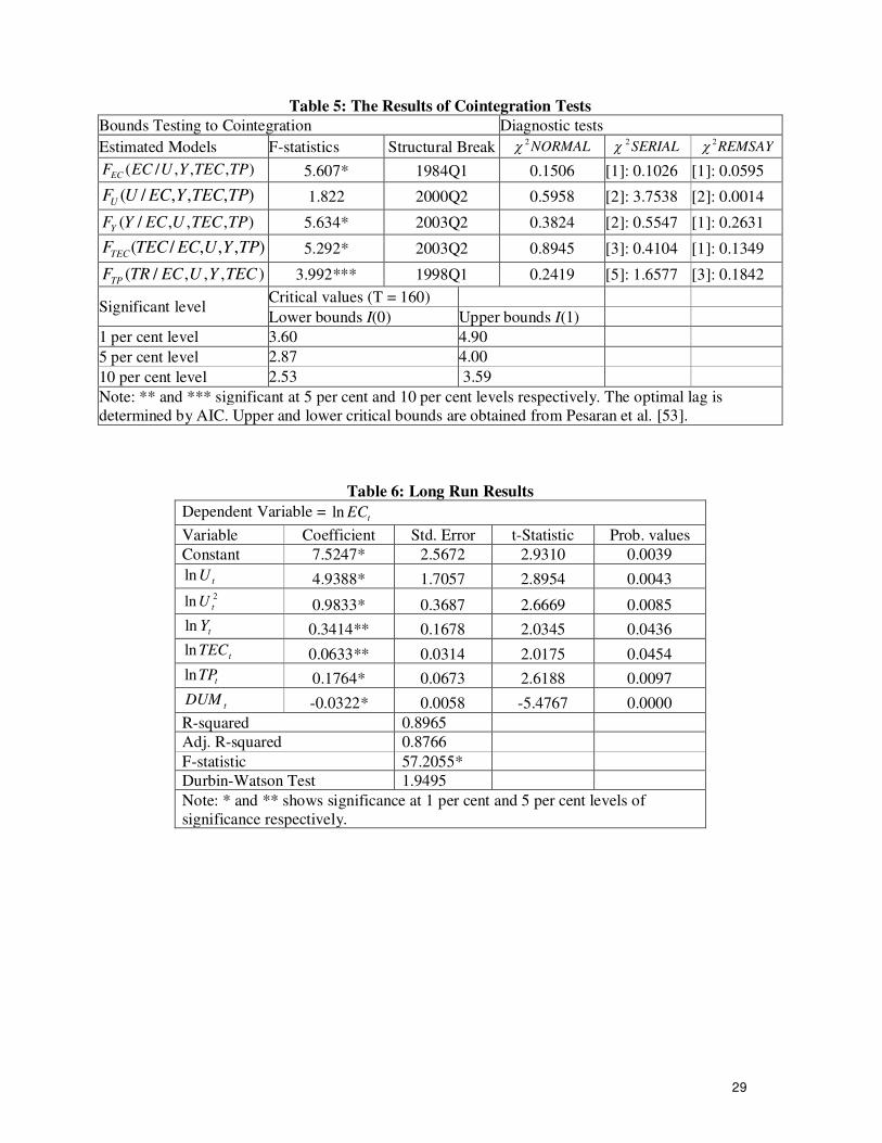
whether long run relationship subsists. We find from the results reported in Table-5 that our
computed F-statistics exceed upper critical bounds at 1% and 5% levels, respectively once we
used energy consumption, economic growth, technology and transportation as dependent
variables. Our empirical evidence shows four cointegrating vectors which confirm the
presence of long run relationship among energy consumption, urbanization, economic
growth, technology and transportation in Pakistan.
[Insert Table 5 here]
The long run impact of urbanization, affluence, technology and transportation on energy
consumption are presented in Table 6. We find that linear and non-linear terms of
urbanization impact energy consumption positively and significantly at 1 per cent level. This
shows that a 1 per cent increase in linear and non-linear terms of urbanization will increase
energy demand by 4.9388 per cent and 0.9833 per cent respectively by keeping other things
constant. Our findings are contradictory with Alam et al. [42], who noted that urbanization is
positively linked to energy consumption via economic growth. Zaman et al. [43] also reported
that urbanization increases electricity consumption in Pakistan, but Jiang and Lin [32] found
inverted U-shaped relationship between urbanization and energy consumption using Chinese
data. The studies conducted by Poumanyvong and Heneko [2], Hossain [61]) and
Poumanyvong et al. [26] supported our findings using the data of cross-country, newly-
industrialized countries and, low, middle and high income countries respectively.
[Insert Table 6 here]
The effect of affluence on energy consumption is positive and significant at 5 per cent. If all
other things remain constant then a 1 per cent add in wealth is associated with 0.3414 per cent
increase in energy demand. This empirical evidence is supported by Alam and Butt [62] who
measured affluence by real GNP per capita and found that affluence leads energy
consumption. The relationship between technology (interaction between industry and services
sectors) and energy demand is positive and significant at 5 per cent level. A 1 per cent
increase in technology adoption to increase domestic output is related to energy demand by
0.0633 per cent, all else is same. This exposes that Rebound Effect does not work in case of
Pakistan. The Rebound effect discloses that “technological improvement will increase energy
efficiency and lower demand of energy resources” [63]. This indicates that Pakistan is using
energy intensive technology, which highlights the importance of enhancing research and
18
development expenditures to introduce energy efficient technology. These results are
contradictory with Linn [64], he found that adoption of advanced technology saves energy via
lowering energy intensity and the same is noted by Popp [65] in the case of the USA.
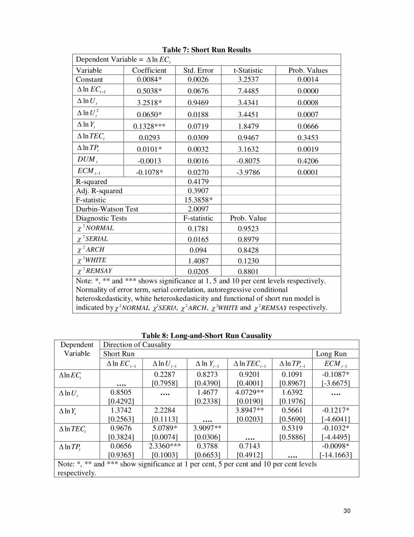
The short run findings are shown in Table 7. The linear and non-linear terms of urbanization
impact energy demand positively and significantly at 1 per cent level. The relationship
between affluence (economic growth) and energy consumption is positive and significant at
10 per cent significance level. The impact of technology adoption is positive but statistically
insignificant. Transportation and energy consumption are positively linked at 1 per cent level
of significance. The negative sign with statistically significance of lagged error term i.e.
1tECM confirms our determined long run relation between the variables.
[Insert Table 7 here]
We find the estimate of 1tECM i.e. -0.1078 with negative sign which is statistically
significant at 1 per cent significance level. Our empirical results indicate that the short run
deviations stem in energy demand function is corrected by 10.78 per cent in each quarter and
will take 2 years and 5 months to achieve stable long run equilibrium path. The short run
model seems to fulfill all assumptions of the classical linear regression model (CLRM). Our
empirical results reported in Table 7. The normal distribution of error term is confirmed by
Jarque-Bera normality test. There is no presence of serial correlation as well as autoregressive
conditional heteroskedisticity in the short run model. The short run model confirms the
existence of homoskedisticity rather than white heteroskedistiity. The Ramsey reset test
provides the evidence of well formulation of the short run model.
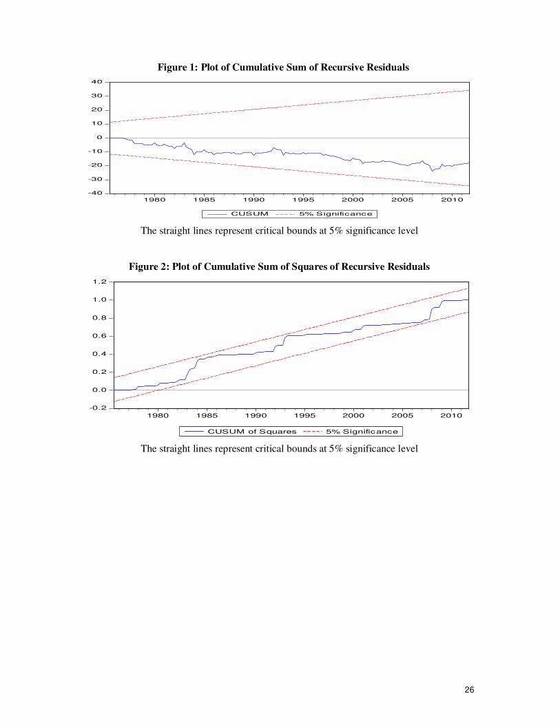
We have applied stability tests such as CUSUM and CUSUMsq to examine the reliability of
long and short run estimates. Pesaran and Shin [66] also suggested to apply CUSUM and
CUSUMsq. We may reject the null hypothesis of CUSUM and CUSUMsq if the plots of both
tests exceed the critical bounds. We may accept null hypothesis which reveal that the model
is well specified if critical bounds remain between critical bounds.
[Insert Figure 1 and 2 here]
19
Both graphs of CUSUM and CUSUMsq are lying between upper and lower limits (see Figure
1 and 2). This leads us to conclude that long and short run estimates are consistent and
reliable. Furthermore, estimates of the ARDL bounds testing are also efficient.
We applied the VECM Granger causality test to detect the causal relationship between
urbanization, affluence, technology, transportation and energy consumption. Our results
reported in Table-8 show that energy consumption is Granger cause of urbanization in the
long run. The feedback effect exists between affluence and energy consumption. It implies
that affluence and energy consumption are complementary and the findings are consistent
with Alam and Butt [62] in the case of Pakistan. It may suggest for the exploration of new
sources of energy supply to sustain long run economic growth.
[Insert Table 8 here]
The causality affiliation between technology and energy demand is bidirectional. This implies
that research and development expenditures must be increased for innovating energy efficient
technologies which in resulting, not only lowers energy intensity but also enhances domestic
production. This empirical evidence is consistent with Tang and Tan [67] who reported the
feedback relationship between technological innovations and energy (electricity) demand in
the case of Malaysia. Transportation Granger causes energy consumption and in resulting,
energy consumption Granger causes transportation. This shows that transportation and energy
consumption are complementary and we can use energy consumption as a tool in forecasting
transportation in Pakistan.
Additionally, urbanization Granger causes affluence (economic growth), technology and
transportation. The feedback hypothesis exists between economic growth and technology.
Economic growth Granger causes transportation and in the resulting, transportation Granger
causes economic growth. The causality relationship between technology and transportation is
also bidirectional. In the short run causality analysis, we find the feedback effect between
urbanization and technology. The feedback hypothesis is validated between affluence and
technology. The unidirectional causality is found running from urbanization to transportation
i.e. urbanization leads transportation.
6. Conclusion and Policy Recommendations
This study deals with impact of urbanization on energy consumption, by incorporating
economic growth, technology and transportation in energy demand function, in Pakistan.
20
Traditional unit root tests such as ADF and PP as well as unit root tests accommodating
structural break stemming in the variables such as Clemente-Montanes-Reyes [56] detrended
unit root test along with NP [51] structural break unit root test were applied in the case of
Pakistan for the period of 1972Q1-2011QQ4. Furthermore, The ARDL bounds testing
approach to cointegration in the presence of structural breaks has been applied to examine
cointegration. The direction of causal relationship between the variables has been investigated
by applying the VECM Granger causality approach.
The empirical results show the presence of cointegration between the variables. Further,
urbanization leads energy consumption (confirmed by both linear and non-linear terms of
urbanization). Affluence (economic growth) raises energy demand. The relationship between
technology and energy consumption is positive. An increase in transportation enhances
energy consumption. The causality analysis shows that energy consumption is Granger cause
of urbanization. Urbanization Granger causes affluence (economic growth), technology and
transportation. The feedback effect exists between energy consumption and affluence.
Technology and transportation are bidirectional Granger caused. The relationship between
technology and affluence is bidirectional and same is true for affluence and transportation.
The bidirectional causality is also found between technology and energy consumption and
same inference is drawn for transportation and energy consumption.
The positive impact of urbanization on energy consumption calls for an important need for
attention of policy makers to meet the challenge of rising energy demand due to rise in urban
population. In such situation, the question is how Pakistan can achieve sustained economic
growth by cutting down energy demand given the bidirectional causality that exists between
economic growth and energy consumption. So, energy demand increases day-by-day due to
increase in per capita income as well as urbanization. Reducing urbanization seems to be a
possible way to control energy demand. However, reduction in urbanization and energy
consumption has detrimental impact on economic growth as urbanization Granger causes
economic growth and feedback effect exists between economic growth and energy
consumption. To support urbanization and hence economic growth as well as
industrialization, there is a need of urban policies to improve urban infrastructure and to bring
into use additional economically feasible sources of energy. In this regard, the investment
opportunities in renewable energy sources should be explored and policies be developed to
encourage such opportunities. The government should build energy efficient urban
21
infrastructure and implement energy saving-projects to decline energy intensity not only at
urban level particularly but also at national level generally. Additionally, energy efficient
policy must be implemented in urban areas to accelerate the switch from high energy
intensive household durables to low energy intensive items.
We find that affluence (economic growth) and technology are positively linked with energy
demand. The government must invest in existing power stations as well as build new power
stations to meet energy demand-supply gap and to dig-out load-shedding. We find that
Pakistan’s industrial and services sector use technology which is energy intensive as
technology is positively related with energy consumption. This implies that government
should pay more attention to allocate more funds for research and development activities to
invent energy efficient technology for industrial and services sectors. This will not only save
energy but also enhance domestic output and hence economic development.
Finally, the relationship between transportation and energy consumption was found positive
as expected. In Pakistan, vehicles (per kilometer of road) were 7 in 2007 but increased to 9 in
2011. The growth of motor vehicles on road is 28.57%. The major share of overall vehicles in
the form of cars and minibus is owned by private sector. The government should implement
rapid bus transit system in all urban areas of the country and banning the use of CNG for car
is not a proper and permanent solution. In this regard, rapid bus transit system should be
implemented in urban areas to meet the rising demand for transportation due to rapid increase
in urban population. The Metrobus system in Lahore is a good example of public transport
facility. Additionally, rapid train transit system should be implemented within cities but also
to connect urban areas of the country following United Kingdom and other European
countries. The trolleybus electric rapid bus system should also be encouraged in urban areas
to reduce fuel consumption and hydropower sources of energy can be used for it. The
hydropower electricity generation is useful for two reasons: (i) hydropower electricity can be
produced at cheaper rate by reducing tariff rates and, (ii), hydropower plants produce clean
energy. The trolleybus electric rapid bus system is cheaper than motorbuses. The non-
motorized modes of transportation such as rapid train transit system and trolleybus electric
rapid bus system are less energy intensive while same is true for Metrobus transit system. The
quality of services must be maintained to attract the people for public transport facility
otherwise allocation of public funds without knowing the source of problem is not good
strategy. So, this would be a possible way to save energy and we can utilize saved energy to
22
meet the rising demand of agriculture, industry and services sectors for sustainable economic
development and better living standard.
References
[1]. Martínez-Zarzoso I. The Impact of Urbanization on CO2 Emissions: Evidence from
Developing Countries. Ibero America Institute for Economic Research; 2008, Universität
Göttingen, Germany.
[2]. Poumanyvong P, Kaneko S. Does Urbanisation Lead to Less Energy Use and Lower CO2
Emissions? A Cross-Country Analysis. Ecological Economics 2010; 70: 434-444.
[3]. World Economic and Social Survey (WESS). World Economic and Social Affairs 2013. [4]. International Energy Agency (IEA) 2012. www.iea.org
[5]. Asian Development Bank (ADB). 2005. Key Indicators 2005. [6].Government of Pakistan. Economic Survey of Pakistan 2010.
[7]. Jones D W. How Urbanisation Affects Energy-use in Developing Countries. Energy Policy 1989; 12: 621-630.
[8]. Dhal C, Erdogan M. Oil Demand in the Developing World: Lessons from the 1980s applied to the 1990s. The Energy Journal 1994; 15: 69-78.
[9]. Burney N A. Socioeconomic Determinants of Electricity Consumption: A Cross-country
Analysis using Coefficient Method. Energy Economics 1995; 17: 185-195.
[10]. Imai H. The Effect of Urbanisation on Energy Consumption. The Journal of Population
Problems 1997; 53: 43-49.
[11]. Cole MA. Neumayer E. Examining the Impact of Demographic Factors on Air
Pollution. Population and Environment 2004; 26: 5-21.
[12]. Kalnay E, Cal M. Impact of Urbanisation and Land-use Change on Climate. Letters to
Nature 2005; 423: 528-531.
[13]. Brant l. The Energy, Economic Growth, Urbanization Nexus across Development:
Evidence from Heterogeneous Panel Estimates Robust to Cross-Sectional Dependence.
The Energy Journal 2013; 34: 223-244.
[14]. Shen L, Cheng S, Gunson JA, Wan H. Urbanization, sustainability and the utilization of
energy and mineral resources in China. Cities 2005; 22: 287–302. [15]. Wang P, Vu W, Zhu B, Wei Y. Examining the impact factors of energy-related
CO2 emissions using the STIRPAT model in Guangdong Province, China. Applied Energy 2013; 106:65-71.
[16]. Mishra V, Smyth R, Sharma S. The Energy-GDP Nexus: Evidence from a Panel of Pacific Island Countries. Resource and Energy Economics 2009; 31: 210-220.
[17]. Lui T. Exploring the Relationship between Urbanisation and Energy Consumption in China using ARDL (Autoregressive Distributed Lag) and FDM (Factor Decomposition
Model). Energy 2009; 34: 1846-1854.
[18]. Zhao-hui L. The Influencing Factors of Energy Consumption under Different Stages of
Urbanization. Journal of Shanghai University of Finance and Economics 2010; 5: 1-5.
[19]. Madlener R, Sunk A. Impact of Urbanisation on Urban Structure and Energy Demand:
What can we Learn for Urban Planning and Urbanisation Management? Sustainable
Cities and Society 2011; 1: 45-53.
[20]. Shahbaz M, Lean H H. Does financial development increase energy consumption? The
role of industrialization and urbanization in Tunisia. Energy Policy 2012; 40: 373-479.
[21]. Islam F, Shahbaz M, Ashraf M U, Alam M M. Financial Development and Energy
Consumption Nexus in Malaysia: A Multivariate Time Series Analysis. Economic
Modelling 2013; 30: 435-441.
23
[22]. Ma H, Du J. Influence of Industrialization and Urbanization on China’s Energy
Consumption. Advanced Materials Research 2012; 524-527: 3122-3128.
[23]. Mickieka, N. M. and Fletcher, J. J. (2012). An Investigation of the Role of China’s
Urban Population on Coal Consumption. Energy Policy. 48, 668-676.
[24]. Toda H Y, Yamamoto T. Statistical Inference in Vector Autoregression with Possible
Integrated Process. Journal of Econometrics 1995; 66: 225-250.
[25]. Zhang C, Lin Y. Panel Estimation for Urbanisation, Energy Consumption and CO2
Emissions: A Regional Analysis in China. Energy Policy 2012; 40: 488-498.
[26]. Poumanyvong P, Kaneko S, Dhakal S. Impact of Urbanisation on National Transport
and Road Energy Use: Evidence from Low, Middle and High Income Countries. Energy
Policy 2012; 46: 208-277.
[27]. Sadorsky P. (2013). Do Urbanization and Industrialization Affect Energy Intensity in Developing Countries? Energy Economics 2013; 37: 52-59.
[28]. Solarin SA, Shahbaz M. (2013). Trivariate Causality between Economic Growth, Urbanisation and Electricity Consumption in Angola: Cointegration and Causality
Analysis. Energy Policy 2013; 60: 876-884. [29]. Pachauri S, Jiang, L. (2008). The Household Energy Transition in India and China.
Energy Policy 2008; 36: 4022-4035. [30]. O'Neill B C, Ren X, Jiang L, Dalton M. The effect of urbanization on energy use in
India and China in the iPETS model. Energy Economics 2012; 34: 339-345.
[31]. Duan J, Yan Y, Zheng B, Zhao J. Analysis of the Relationship between Urbanisation
and Energy Consumption in China. International Journal of Sustainable Development &
World Ecology 2008; 15: 309-317.
[32]. Jiang Z, Lin B. China’s Energy Demand and its Characteristics in the Industrialization
and Urbanisation Process. Energy Policy 2012; 49: 608-615.
[33]. Zhang S, Qin X. Comment on “China’s Energy Denand and its Characteristics in the
Industrialisation and Urbanisation Process” by Zhujun Jiang and Boqiang Lin. Energy
Policy 2013; 59: 942-945.
[34]. Xia X H, Hu Y. Determinants of Electricity Consumption Intensity in China: Analysis
of Cities at Sub-province and Prefecture Levels in 2009. The Scientific World Journal
2012; 12: 1-12.
[35]. Apergis N, Tang C F. Is the Energy-Led Growth Hypothesis Valid? New Evidence from Sample of 85 Countries. Energy Economics 2013; 38: 24-31.
[36]. Dolado JJ, Lütkepohl H. Making Wald Tests Work for Cointegrated VAR Systems. Econometric Review 1996; 15: 369-386.
[37]. Pedroni P. (2004). Panel Cointegration: Asymptotic and Finite Sample Properties of Pooled Time Series Tests with an Application to the PPP Hypothesis. Econometric
Theory 2004; 20: 597-625. [38]. Liu Y, Xie Y. Asymmetric Adjustment of the Dynamic Relationship between Energy
Intensity and Urbanization in China. Energy Economics 2013; 36: 43-54.
[39]. Wang Q. Effects of Urbanization on Energy Consumption in China. Energy Policy
2014; 65: 332-339.
[40]. Lidlle B, Lung S. (2013). Might Electricity Consumption Cause Urbanization instead?
Evidence from Heterogeneous Panel Long-run Causality Tests. Global Climate Change
2013; 24: 42-51.
[41]. Shahbaz M, Loganathan N, Sbia R, Afza T. The effect of urbanization, affluence and
trade openness on energy consumption: A time series analysis in Malaysia. Renewable
and Sustainable Energy Reviews 2015; 47: 683-693.
24
[42]. Alam S, Fatima A, Butt M M. Sustainable Development in Pakistan in the Context of
Energy Consumption Demand and Environmental Degradation. Journal of Asian
Economics 2007; 18: 825-837.
[43]. Zaman K, Khan M M, Ahmad M, Rustem R. Determinants of Electricity Consumption
Function in Pakistan: Old Wine in New Bottle. Energy Policy 2012; 50: 623-634.
[44]. Ali G, Nitivattananon V. Exercising multidisciplinary approach to assess
interrelationship between energy use, carbon emission and land use change in a
metropolitan city of Pakistan. Renewable and Sustainable Energy Reviews 2012; 16: 775-
786.
[45]. Liddle B. Demographic Dynamics and Per Capita Environmental Impact: Using Panel
Regressions and Household Decompositions to Examine Population and Transport.
Population and Environment 2004; 26: 23-39. [46]. Hemmati A. A Change in Energy Intensity: Test of Relationship between Energy
Intensity and Income in Iran. Iranian Economic Review 2006; 11: 123-130. [47]. Zhou W, Zhu B, Chen D, Griffy-Brown C, Ma Y, Fei W. (2011). Energy consumption
patterns in the process of China’s urbanization. Population and Environment 2011; 33: 202-220.
[48]. World Development Indicators, World Bank 2013. [49]. Romero A M. Comparative Study: Factors that Affect Foreign Currency Reserves in
China and India 2005). Honors Projects. Paper 33, Illinois Wesleyan University, United
States.
[50]. McDermott J, McMenamin P. Assessing Inflation Targeting in Latin America with a
DSGE Model. Central Bank of Chile Working Papers, N° 469, Chile 2008.
[51]. Narayan PK, Popp S. A New Unit Root Test with Two Structural Breaks in the Level
and Slope at Unknown Time. Journal of Applied Statistics 2010; 37: 1425-1438.
[52]. Johansen S, Juselies K. Maximum Likelihood Estimation and Inferences on Co-
integration. Oxford Bulletin of Economics and Statistics 1990; 52: 169-210.
[53]. Pesaran M H, Shin Y, Smith R. Bounds Testing Approaches to the Analysis of Level
Relationships. Journal of Applied Econometrics 2001; 16: 289-326.
[54]. Laurenceson J, Chai JCH. Financial Reform and Economic Development in China.
Cheltenham, UK, Edward Elgar 2003.
[55]. Narayan PK. The Saving and Investment Nexus for China: Evidence from Cointegration Tests. Applied Economics 2005; 37: 1979-1990.
[56]. Clemente J, Montañés A, Reyes M. Testing for a unit root in variables with a double change in the mean. Economics Letters 1998; 59: 175-182.
[57]. Masih A, Masih R. A Comparative analysis of the propagation of stock market fluctuations in alternative models of dynamic causal linkages. Applied Financial
Economics 1997; 7: 59-74. [58]. Granger CW J. Investigating Causal Relations by Econometric Models and Cross-
Spectral Methods. Econometrica 1969; 37: 424-438.
[59]. Dejong D N, Nankervis J C, Savin N E. Integration versus trend stationarity in time
series. Econometrica 1992; 60: 423-33.
[60]. Elliot G, Rothenberg T J, Stock J H. Efficient tests for an autoregressive unit root.
Econometrica 1996; 64: 813-836.
[61]. Hossain M S. Panel Estimation for CO2 Emissions, Energy Consumption, Economic
Growth, Trade Openness and Urbanisation of Newly Industrialized Countries. Energy
Policy 2011; 39: 6991-6999.
[62]. Alam S, Butt M S. Causality between Energy and Economic Growth in Pakistan: An
Application of Cointegration and Error-correction Modeling Techniques. Pacific and
Asian Journal of Energy 2002; 12: 151-165.
25
[63]. Keppler JH, Bourbannouis R, Girod J. (2007). The Econometrics of Energy Systems,
New York; Palgrave Macmillan.
[64]. Linn J. Energy Prices and the Adoption of Energy-Saving Technology. The Economic
Journal 2008;118: 1986-2012.
[65]. Popp DC. The Effect of New Technology on Energy Consumption. Resource and
Energy Economics 2001; 23: 215-239.
[66]. Pesaran and Shin (1999)
[67]. Tang C F, Tan E C. Exploring the Nexus of Electricity Consumption, Economic
Growth, Energy Prices and Technology Innovation in Malaysia. Applied Energy 2013;
104: 297-305.
26
Figure 1: Plot of Cumulative Sum of Recursive Residuals
-40
-30
-20
-10
0
10
20
30
40
1980 1985 1990 1995 2000 2005 2010
CUSUM 5% Significance
The straight lines represent critical bounds at 5% significance level
Figure 2: Plot of Cumulative Sum of Squares of Recursive Residuals
-0.2
0.0
0.2
0.4
0.6
0.8
1.0
1.2
1980 1985 1990 1995 2000 2005 2010
CUSUM of Squares 5% Significance
The straight lines represent critical bounds at 5% significance level
27
Table 1: Descriptive Statistics and Correlation Matrix
Variables tECln tUln tYln tTECln tTPln
Mean 4.5701 -1.1740 10.0384 4.2488 1.9334
Median 4.5977 -1.1716 10.0960 4.3635 2.0047
Maximum 4.8846 -0.9879 10.4573 5.3350 2.4756
Minimum 4.2376 -1.3736 9.5749 2.9566 1.0885
Std. Dev. 0.1967 0.1091 0.2629 0.6904 0.3988
Skewness -0.1045 -0.0494 -0.1815 -0.1555 -0.4907
Kurtosis 1.7101 2.0072 1.9808 2.0196 2.1333
Jarque-Bera 2.9236 1.6589 1.9507 1.7630 2.8572
Probability 0.2318 0.4362 0.3770 0.4141 0.2396
Observation 160 160 160 160 160
tECln 1.0000
tUln 0.1546 1.0000
tYln 0.4356 0.0108 1.0000
tTECln 0.4518 0.1772 0.7035 1.0000
tTPln 0.0164 0.3045 0.1074 0.2452 1.0000
Tsable 2: Unit Root Tests without Structural Break
Variables Augmented Dickey-Fuller Test Philips-Perron Test
T-statistics Prob. Values T-statistics Prob. Values
tECln -2.6542(9) 0.2573 -2.3110 [3] 0.3252
tUln -2.1212 (9) 0.5593 -2.7789 [3] 0.2073
tYln -2.1353 (9) 0.5216 -1.7322 [6] 0.7324
tTECln -2.1496 (4) 0.3134 -2.1255 [6] 0.5256
tTPln -3.0510 (6) 0.1221 -26.9119 [15]* 0.0000
tECln -3.7551 (8)** 0.0216 -6.7525 [6]* 0.0000
tUln -4.8647 (7)* 0.0006 -6.7551 [6]* 0.0000
tYln -3.7990 (4)** 0.0191 -6.0931 [6]* 0.0000
tTECln -3.5907 (4)** 0.0339 -5.3757 [6]* 0.0001
tTPln -5.5168 (9) * 0.0000 -5.2394 [6]* 0.0001
Note: * and ** show significance at 1 per cent and 5 per cent respectively. () and [] indicate lag order and bandwidth based on AIC for ADF and PP unit root tests
respectively.
28
Table 3: Unit Root Tests with Structural Break
Clemente-Montanes-Reyes Detrended Structural Break Unit Root Test
Variable Innovative Outliers Additive Outlier
T-statistic TB1 TB2 T-statistic TB1 TB2
tECln
-2.013 (6) 1984Q1 …. -5.059 (3)* 1985Q1 ….
-3.800(6) 1985Q1 2001Q2 -5.373 (5)** 1986Q1 2001Q1
tUln
-2.808 (3) 2000Q2 …. -4.713 (6)** 2006Q1 ….
-3.525 (6) 1996Q2 2006Q2 -5.672 (6)* 1979Q1 2006Q1
tYln
-1.885 (6) 2003Q2 …. -6.896 (3)* 1980Q2 ….
-4.867 (2) 1979Q1 2003Q1 -8.611 (3)* 1992Q1 2001Q1
tTECln
-2.285 (6) 2003Q2 …. -6.619 (3)* 2007Q1 ….
-4.468 (3) 1977Q1 2003Q1 -7.641 (3)* 2003Q1 2007Q1
tTPln
-3.313 (4) 1999Q1 …. -7.715 (6)* 2006Q2 ….
-4.194 (5) 1976Q1 1996Q1 -7.735 (5)* 1999Q1 1999Q3
Narayan and Popp Structural Break Unit Root Test
Variables Model M1 Model M2
tECln -2.0597 (4) 1987Q1 2004Q1 -2.2927 (5) 1987Q1 2004Q1
tUln
-1.549 (5) 1995Q4 2001Q2 -2.252 (5) 1995Q4 2001Q2
tYln -2.673 (5) 1999Q1 2005Q4 -3.190 (4) 1994Q4 2004Q2
tTECln
-1.679 (5) 1978Q1 1987Q4 -3.341 (4) 1988Q4 2001Q3
tTPln -3.208 (4) 1983Q4 1990Q2 -4.319 (5) 1983Q4 1998Q3
Note: * and ** significant at 1 per cent and 5 per cent levels respectively. () indicates lag length
to be used. The critical values of NP unit root test are (-5.259, -5.949) and (-4.154, -5.181) for
Model M1 and Model M2 at 1 per cent and 5 per cent levels respectively.
Table 4: VAR Lag Order Selection Criteria
VAR Lag Order Selection Criteria
Lag LogL LR FPE AIC SC HQ
1 3497.793 4074.022 1.05e-26 -45.6288 -45.0320 -45.3864
2 3677.301 333.0358 1.38e-27 -47.6618 -46.5676 -47.2173
3 3691.350 25.1387 1.59e-27 -47.5177 -45.9262 -46.8712
4 3697.798 11.1156 2.05e-27 -47.2736 -45.1848 -46.4250
5 3836.501 229.9551 4.62e-28 -48.7697 -46.1835 -47.7191
6 3984.881 236.2364* 9.22e-29* -50.393* -47.3096* -49.1405*
7 3994.246 14.2930 1.15e-28 -50.1874 -46.6065 -48.7327
8 3998.132 5.67561 1.56e-28 -49.9096 -45.8313 -48.2529
* indicates lag order selected by the criterion
LR: sequential modified LR test statistic (each test at 5% level)
FPE: Final prediction error
AIC: Akaike information criterion
SC: Schwarz information criterion
HQ: Hannan-Quinn information criterion
29
Table 5: The Results of Cointegration Tests
Bounds Testing to Cointegration Diagnostic tests
Estimated Models F-statistics Structural Break
NORMAL2 SERIAL2 REMSAY2
),,,/( TPTECYUECFEC 5.607* 1984Q1 0.1506 [1]: 0.1026 [1]: 0.0595
),,,/( TPTECYECUFU 1.822 2000Q2 0.5958 [2]: 3.7538 [2]: 0.0014
),,,/( TPTECUECYFY 5.634* 2003Q2 0.3824 [2]: 0.5547 [1]: 0.2631
),,,/( TPYUECTECFTEC 5.292* 2003Q2 0.8945 [3]: 0.4104 [1]: 0.1349
),,,/( TECYUECTRFTP
3.992*** 1998Q1 0.2419 [5]: 1.6577 [3]: 0.1842
Significant level Critical values (T = 160)
Lower bounds I(0) Upper bounds I(1)
1 per cent level 3.60 4.90
5 per cent level 2.87 4.00
10 per cent level 2.53 3.59
Note: ** and *** significant at 5 per cent and 10 per cent levels respectively. The optimal lag is
determined by AIC. Upper and lower critical bounds are obtained from Pesaran et al. [53].
Table 6: Long Run Results
Dependent Variable = tECln
Variable Coefficient Std. Error t-Statistic Prob. values
Constant 7.5247* 2.5672 2.9310 0.0039
tUln 4.9388* 1.7057 2.8954 0.0043 2ln tU 0.9833* 0.3687 2.6669 0.0085
tYln 0.3414** 0.1678 2.0345 0.0436
tTECln 0.0633** 0.0314 2.0175 0.0454
tTPln 0.1764* 0.0673 2.6188 0.0097
tDUM
-0.0322* 0.0058 -5.4767 0.0000
R-squared 0.8965
Adj. R-squared 0.8766
F-statistic 57.2055*
Durbin-Watson Test 1.9495
Note: * and ** shows significance at 1 per cent and 5 per cent levels of
significance respectively.
30
Table 7: Short Run Results
Dependent Variable = tECln
Variable Coefficient Std. Error t-Statistic Prob. Values
Constant 0.0084* 0.0026 3.2537 0.0014
1ln tEC 0.5038* 0.0676 7.4485 0.0000
tUln 3.2518* 0.9469 3.4341 0.0008
2lnt
U 0.0650* 0.0188 3.4451 0.0007
tYln 0.1328*** 0.0719 1.8479 0.0666
tTECln 0.0293 0.0309 0.9467 0.3453
tTPln 0.0101* 0.0032 3.1632 0.0019
tDUM -0.0013 0.0016 -0.8075 0.4206
1tECM -0.1078* 0.0270 -3.9786 0.0001
R-squared 0.4179
Adj. R-squared 0.3907
F-statistic 15.3858*
Durbin-Watson Test 2.0097
Diagnostic Tests F-statistic Prob. Value
NORMAL2 0.1781 0.9523
SERIAL2 0.0165 0.8979
ARCH2 0.094 0.8428
WHITE2 1.4087 0.1230
REMSAY2 0.0205 0.8801
Note: *, ** and *** shows significance at 1, 5 and 10 per cent levels respectively.
Normality of error term, serial correlation, autoregressive conditional
heteroskedasticity, white heteroskedasticity and functional of short run model is
indicated by NORMAL2 , SERIAL2 , ARCH2 , WHITE2 and REMSAY2 respectively.
Table 8: Long-and-Short Run Causality
Dependent
Variable
Direction of Causality
Short Run Long Run
1ln t
EC 1ln t
U 1ln t
Y 1ln t
TEC 1ln t
TP 1tECM
tECln ….
0.2287
[0.7958]
0.8273
[0.4390]
0.9201
[0.4001]
0.1091
[0.8967]
-0.1087*
[-3.6675]
tUln 0.8505
[0.4292]
….
1.4677
[0.2338]
4.0729**
[0.0190]
1.6392
[0.1976]
….
tYln 1.3742
[0.2563]
2.2284
[0.1113] ….
3.8947**
[0.0203]
0.5661
[0.5690]
-0.1217*
[-4.6041]
tTECln 0.9676
[0.3824]
5.0789*
[0.0074]
3.9097**
[0.0306] ….
0.5319
[0.5886]
-0.1032*
[-4.4495]
tTPln 0.0656
[0.9365]
2.3360***
[0.1003]
0.3788
[0.6653]
0.7143
[0.4912] ….
-0.0098*
[-14.1663]
Note: *, ** and *** show significance at 1 per cent, 5 per cent and 10 per cent levels
respectively.