Munich Personal RePEc Archive - uni-muenchen.de · 0 3 5 $ Munich Personal RePEc Archive Money Demand and In ation: A Cointegration Analysis for Canada Federico Lubello Department

MPRAMunich Personal RePEc Archive

Money Demand and Inflation: ACointegration Analysis for Canada

Federico Lubello

Department of Economics and Finance, Catholic University of Milan

July 2011

Online at https://mpra.ub.uni-muenchen.de/54960/MPRA Paper No. 54960, posted 1 April 2014 10:56 UTC

http://mpra.ub.uni-muenchen.de/

https://mpra.ub.uni-muenchen.de/54960/

Money Demand and Inflation: ACointegration Analysis for Canada

Federico Lubello⇤

July 2011

Abstract

The aim of this paper is to investigate the presence of long-run equilibrium relation-ships among variables that explain money demand in Canada during the period 1983–2011.To this end, I set up a vector-error correction model with an appropriate lag order and testfor cointegration by means of the Bartlett corrected trace test. I estimate the long-runmoney demand parameters by means of the maximum likelihood method of Johansen,comparing an unconstrained benchmark model against a constrained model. I find thelatter to not be better than the benchmark one. Finally, I perform sensitivity analysis andcheck the stability of the resulting cointegration relationships.

JEL classification: C3; E31; E41

Keywords: Canada, cointegration, money demand, vector autoregression, VECM

⇤Department of Economics and Finance, Catholic University of Milan, Largo Gemelli, 1,20123 Milan, Italy. E-mail: [email protected]

1 Theoretical background

This empirical work aims at investigating the presence of cointegrating relation-ships among the variables that explain money demand in Canada. Cointegrationarises when two non–stationary series have in common the same stochastic trend.In particular, let us consider two series, Yt and Xt , integrated of order one andsuppose that a linear relation between them exists. If there exists some value of bsuch that Yt �bXt is integrated of order zero, then it is said that Yt and Xt are coin-tegrated and that they share a common trend. In this work, I will explore whetherand to which extend such a relation exists between the determinants of Canadianmoney demand. The set of variables considered are:

mt : log of real M1 money balancesin f lt : quarterly inflation rate (in % per year)cprt : commercial paper rateyt : log real GDP (in billions of 2002 dollars)trbt : treasury bill rate.

The commercial paper rate and the treasury bill rate are considered as riskyand risk-free returns, respectively. The series for M1 and GDP are seasonallyadjusted.

In principle, we could dispute the presence of a unit root in some of theseseries. As customary in the literature, I assume that these variables are well de-scribed by an I(1) process. One can think of three possible cointegrating relation-ships governing the long-run behavior of these variables. First, we can specifymoney demand as

mt = a1 +b14yt +b15tbrt + e1t (1)

where b14 denotes the income elasticity and b15 the interest rate elasticity. It canbe expected that it is close to unity, corresponding to a unitary income elasticity,and that b15 < 0. Second, if real interest rate is stationary we can express an

Money Demand and Inflation in Canada: A Cointegration Analysis 3

equation for inflation

in f lt = a2 +b25tbrt + e2t (2)

which corresponds to a cointegrating relationship with b25 = 1 . This is referred toas the Fisher equation where we are using actual inflation as a proxy for expectedinflation. Third, we can expect the risk-premium to be stationary so that a thirdcointegrating relationship can be expressed as

cprt = a3 +b35tbrt + e3t (3)

with b 35 = 1.

2 Empirical analysis

The data have been collected on a quarterly horizon for the period ranging be-tween June 1983:2 to March 2011:2. The total number of observation equals112. 1 Relaying on the literature we can expect our variables to be stationary,but following Hoffman and Rasche (1996) let us assume for them to be I(1) andtherefore that they turn to be stationary after taking their first differences. Themore standard way to test the presence of unit root is the Dicky-Fuller test andits augmented version. For comparison, in Table (1) are reported these tests per-formed on the original series and in Table (2) the same analysis performed on thetheir first differences.

Before proceeding to the vector error-correction process of these five vari-ables, let me consider the OLS estimates of the above three regressions, which

1The data have been collected from the National Bureau Statistics of Canada:http://www.statcan.gc.ca/


Table 1: Dicky-Fuller test I(1)

mt in f lt cprt yt tbrt

DF -1.241 -3.163 ** -1.163 -2.018 -0.904

ADF (6) -0.117 -1.993 -1.993 -0.547 -1.638

*** 1%, ** 5%, * 10%

Table 2: Dicky-Fuller Test First Difference

mt in f lt cprt yt tbrt

DF -6.671 *** -10.689 *** -9.971 *** -5.545 *** -8.422 ***

ADF (6) -3.137 ** -3.917 *** -3.955 *** -3.273 ** -4.443 ***

are presented in Table (3) and show that with the exception for the Fisher equa-tion, both money demand and risk-premium have an R2 close to unity which isan informal requirement for a cointegration relationship. In addition, we can testfor cointegration by means of the usual Durbin–Watson statistic. Under the nullhypothesis of a unit root, the appropriate test is wether DW is significantly largerthan zero (Verbeek, 2004). Given the standards critical values, we should rejectthe null hypothesis for risk-premium and Fisher equations but not for money de-mand. However, these results have to be considered only partially reliable sincethe test is based on the random walk assumption for the data generating processof all series, that is not the case for the GDP and money supply which are clearlytrended-series. Nevertheless, the value of the Durbin–Watson statistics is oftenuseful to obtain a general idea about wether or not a cointegrating relationshipmight exist.

We can also test for a unit root in the residuals of the regressions by meansof the augmented Dickey-Fuller tests. The results, for 6 lags, are also reported inTable (3).


Table 3: Univariate cointegrating regressions by OLS (standard errors in paren-theses), intercept estimates not reported.

Money Demand Fisher Equation Risk-premium

mt -1 0 0

in f lt 0 -1 0

cprt 0 0 -1

yt 2.727 (0.062) 0 0

tbrt -2.822 (0.399 ) 0.323 (0.029) 0.974 (0.011)

R2 0.9868 0.527 0.986

dw 0.108 0.577 1.770

ADF (6) -1.988 -2.376 -4.100

Given the 5% asymptotic critical values of -3.37 and -3.77 for the regressioninvolving three and two variables respectively, we can reject the null hypothesis ofno cointegration only for the risk-premium equation. Given the results obtainedup to now, it is not that straightforward to state something about the presence ofcointegration relationships between our variables. Recalling that cointegration re-quires R2 values close to unity, high values of the DW test and no serial correlationin regression residuals, our results show that these requirements are only partiallyfulfilled, and even when they are it is not the case always for the same variablesat the same time, providing results that are therefore mixed. In fact, summing upwe obtain R2 values close to unity for money demand and risk-premium equationsand sufficiently high DW and ADF values only for the risk-premium equation. Inorder to get additional information it may be useful to plot the residuals of thethree regressions. We can interpret cointegration as long-run stable equilibrium,so that regression residuals should therefore look like a stationary mean reverting


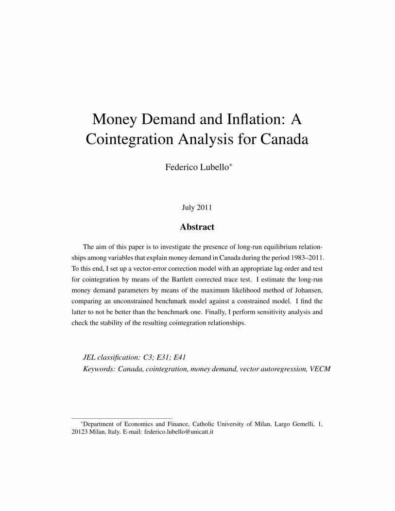
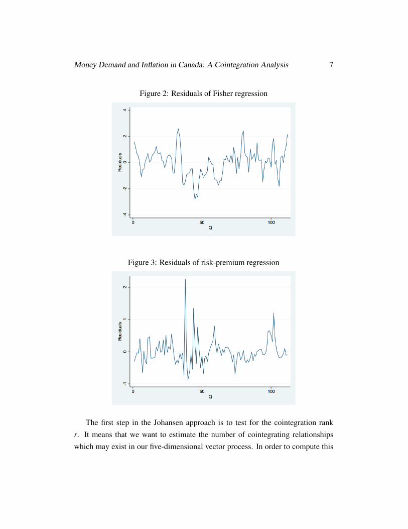
process fluctuating around zero. The residuals of the three regressions are dis-played in Fig.(1), Fig.(2) and Fig.(3), respectively. However, in our case we canobserve by visual inspection only some evidence of mean reversion for the Fisherequation and the risk-premium equation, but there is less evidence for money de-mand.

Figure 1: Residuals of money demand regression


Figure 2: Residuals of Fisher regression

Figure 3: Residuals of risk-premium regression

The first step in the Johansen approach is to test for the cointegration rankr. It means that we want to estimate the number of cointegrating relationshipswhich may exist in our five-dimensional vector process. In order to compute this


tests, we first need to choose how many lags (lags length p) to be used in thevector error-correction model. This can be obtained by means of a specific test,which provide the lag-order selection statistics for our VECM, at a pre-estimationlevel. As it can be seen in Table (4), the Akaike information criterion, the Hannan-Quinn information criterion and the final prediction error jointly suggest to selectas optimal lag-order p = 2. However, the existing literature suggest that choosingp too small will invalidate results and choosing p too high may results in loss ofpower (Veerbeek, 2004). For this reasons, I found it more optimal to choose avalue of p = 4 2.

Table 4: Lag-Order Selection Statistics

Lag LL LR df p FPE AIC HQIC SBIC0 1138.73 1.5e-16 -22.2301 -22.178 -22.10141 1812.65 1347.8 25 0.000 4.5e-22 -34.9539 -34.6413 -34.1818*2 1859.32 93.337 25 0.000 3.0e-22* -35.3788* -34.8056* -33.96333 1869.51 20.382 25 0.727 4.0e-22 -35.0884 -34.2547 -33.02964 1890.93 42.853 25 0.015 4.4e-22 -35.0183 -33.9241 -32.31625 1924.37 66.864 25 0.000 3.8e-22 -35.1837 -33.8289 -31.83816 1946.17 43.608 25 0.012 4.2e-22 -35.121 -33.5057 -31.13217 1974.44 56.545 25 0.000 4.2e-22 -35.1852 -33.3094 -30.55298 1995.26 41.626 25 0.020 5.0e-22 -35.1031 -32.9668 -29.82749 2022.64 54.772 25 0.01 5.3e-22 -35.1499 -32.753 -29.2308

10 2048.43 51.574* 25 0.01 6.0e-22 -35.1653 -32.5079 -28.6028

Endogenous: cpr infl tbr logdp logm1Exogenous: _consMaxlag(10)

After having determined the optimal lags length p = 4, I proceed to the de-termination of the number of cointegrating relationships to be used for the error-

2Analysis performed by using p = 2 displayed highly correlated residuals. I then have selectedp = 4, which is closer to the value chosen in literature for the same typology of data and analysis.


correction model estimation. The tests for cointegration are based on Johansen’smethod. If the log likelihood of the unconstrained model that includes the coin-tegrating equations is significantly different from the log likelihood of the con-strained model that does not include the cointegrating equations, we reject thenull hypothesis of no cointegration. Results are provided in Table (5) indicatingthe presence of two cointegrating relationships.

Table 5: Johansen’s Cointegration Test

Max Rank Parms LL Eigenvalue Trace Statistic 5% Critic. Value

0 105 -1456.567 . 105.1762 68.52

1 114 -1432.6779 0.36015 57.3981 47.21

2 121 -1418.598 0.23139 29.2383 * 29.68

3 126 -1411.9966 0.11608 16.0353 15.41

4 129 -1406.8365 0.09194 5.7153 3.76

5 130 -1403.9789 0.05201 - -

To identify individual cointegrating relationships I need to normalize the coin-tegrating vectors. Since r = 2, I need to impose two normalization constraints oneach cointegrating vector. In this case, I impose mt and cprt to have coefficientsof �1, 0 and 0, �1, respectively in each constraint. I shall estimate the cointe-grating vectors by maximum likelihood jointly with the coefficients in the vectorerror-correction model, which takes the following general form:

ecmi = a0 +bi1mt +bi2in f lt +bi3cprt +bi4yt +bi5tbrt (4)


With the restrictions imposed above we therefore have: b11 = �1 , b13 = 0and b21 = 0, b23 =�1. After estimation, I get the results reported in Table (6).

Table 6: ML estimates of cointegrating vectors (after normalization) based onVAR with p = 4 (standard errors in parentheses), intercept estimates not reported.

Money demand Risk-premium

mt -1 0

in f lt 22.283 (5.638) 0.238 (0.108)

cprt 0 -1

yt 0.627 (0.477) -0.292 (0.009)

tbrt -22.576 (3.939) 0.710 (0.076)

Log likelihood value: 1975.709

For a fair interpretation of these results, and in order to determine which vari-ables enter actually the equations and which ones do not, I need to check the sig-nificance of their coefficients. It is possible to do this by means of the t-statistics.They are reported in Table (7). With regards to the cointegrating vector corre-sponding to the risk premium equation, I reject the null hypothesis for for allcoefficients to be zero, and they are therefore significantly different from zero.This means that all the variables involved in the risk premium relation are con-tributing significantly in determining that relation. In addition, I also reject thenull hypothesis for the treasury bills rate coefficient to be equal to one, so that oura priori expectations (see Table 3) are not confirmed. Regarding the cointegrat-ing vector corresponding to the money demand equation, I cannot reject the nullhypothesis only for the output coefficient. Therefore, both inflation and treasurybills rate enter significantly into the money demand equation. This contradicts oura priori expectations (again Table 3) where inflation is not entering the equation.


Table 7: T-Statistics based on Table (6)

Money demand Risk premium

mt - -

in f lt 3.952 2.204

cprt - -

yt 1.314 -32.444

tbrt -5.731 9.342

I can also test our a priori cointegrating vectors by using likelihood ratio testsand by imposing additional constraints on the cointegration vectors, which are:

Ha0 : b12 = 0, b14 = 1;

Hb0 : b22 = b24 = 0, b25 = 1;

Hc0 : b12 = b22 = b24 = 0, b14 = b25 = 1,

The model is estimated testing all three hypotheses. In Table (8) the likelihoodvalues and the likelihood ratio tests for each case are reported.

Table 8: ML estimates for the complete a priori model

Log-likelihood values Likelihood Ratio Tests

Ha0 1970.345 10.728

Hb0 1969.139 13.14

Hc0 1971.329 8.76

The likelihood ratios are defined as twice the difference between the Like-lihood of the estimated model (constrained) and the benchmark (unconstrained)one. The asymptotic distribution under the null hypotheses are the Chi-squared


Figure 4: Residuals of the Original Model

distributions with degrees of freedom given by the number of restrictions that Ihave imposed. In the present case, I imposed two restrictions on coefficients inHa

0 , three in Hb0 and five in Hc

0 . The Chi-squared critical values for 2, 3 and 5degrees of freedom are 5.991, 7.815 and 11.070, respectively and therefore I canonly reject Hc

0 meaning that the unconstrained model is as good as the uncon-strained one and not better. In order to evaluate the original model, I can performadditional residual analysis and plotted in Fig. (4) .

In Fig. (5) it is shown the periodgramm as a result of the Bartlett’s test, whichtests the null hypothesis that the data come from a white-noise process of uncorre-lated random variables having a constant mean and a constant variance. I can seein the graph below that the values never appear outside the confidence bands. Thetest statistic has a p-value of 0.81, so I conclude that the process is not differentfrom a white noise.


Figure 5: White Noise Test

In addition, I perform a test for autocorrelation in the residuals of vector error-correction model. The test implements Lagrange-multiplier (LM) test for auto-correlation in the residuals of vector error-correction model where for each lag jthe null hypothesis of the test is that there is no autocorrelation at a specific lagj. From results, reported in Table (9), it can be realized that we cannot rejectthe null hypothesis of no autocorrelation from the second lag toward, but in thefirst lag the serial correlation is statistically significant. At this point, in order todetermine whether this autocorrelation coefficient is statistically close to 1, I canregress residuals on lags. Results show a coefficient equal to 0.0057 and a stan-dard error of 0.0969, so that calculating the appropriate t-ratio it turns out to bedifferent then 1.


Table 9: Lagrange Multipliers Test

Lag Chi2 df Prob>Chi2

1 55.0209 25 0.000492 21.2437 25 0.678953 31.3888 25 0.176464 52.3511 25 0.001085 26.4747 25 0.382636 40.6415 25 0.025037 24.9622 25 0.464508 22.0622 25 0.632159 19.7791 25 0.75831

10 23.5782 25 0.5438411 31.8810 25 0.1614812 30.2011 25 0.21685

Some consideration may be done about the stability conditions of VECM es-timates. I perform a test that provides indicators of whether the number of coin-tegrating equations is misspecified or whether the cointegrating equations, whichare assumed to be stationary, are not stationary. From the test I expect to obtainthat the number of eigenvalues having unit moduli is equal to K � r, that is thedifference between the number of variable K and the number of cointegrating re-lationships r. The results of this analysis reported in Table (10) confirm theseexpectations.


Table 10: Eigenvalue Stability Condition

Eigenvalue Modulus1 11 11 1

0.7529544 + 0.2866931i 0.8056880.7529544 - 0.2866931i 0.805688

0.756527 0.7565270.6470258 + 0.3871149i 0.753990.6470258 - 0.3871149i 0.75399

-0.4473219 + 0.5838522i 0.735514-0.4473219 - 0.5838522i 0.735514-0.1979945 + 0.5781694i 0.611131-0.1979945 - 0.5781694i 0.611131

0.6047231 0.6047230.02288368 + .5999055i 0.6003420.02288368 - 0.5999055i 0.600342-0.357975 + 0.3968059i 0.534416

-.357975 - .3968059i 0.534416-.1759097 + .2917176i 0.340651-.1759097 - .2917176i 0.340651

-.1168251 0.116825

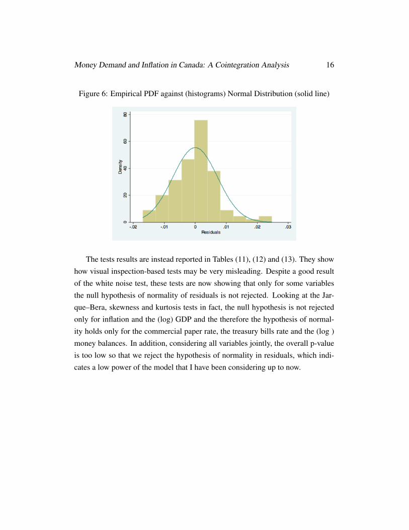
Moreover, I perform a further test to check normality of residuals which in-volves Jarque-Bera, Skewness and Kurtosis tests. For a first visual inspectionabout these statistical properties, it would be useful to have a look to Fig. (6)where the empirical probability distribution function (PDF) of residuals is plottedagainst the normal probability density function.


Figure 6: Empirical PDF against (histograms) Normal Distribution (solid line)

The tests results are instead reported in Tables (11), (12) and (13). They showhow visual inspection-based tests may be very misleading. Despite a good resultof the white noise test, these tests are now showing that only for some variablesthe null hypothesis of normality of residuals is not rejected. Looking at the Jar-que–Bera, skewness and kurtosis tests in fact, the null hypothesis is not rejectedonly for inflation and the (log) GDP and the therefore the hypothesis of normal-ity holds only for the commercial paper rate, the treasury bills rate and the (log )money balances. In addition, considering all variables jointly, the overall p-valueis too low so that we reject the hypothesis of normality in residuals, which indi-cates a low power of the model that I have been considering up to now.


Table 11: Jarque-Bera Test

Equation Chi2 df Prob>Chi2D_cpr 7.624 2 0.02210D_inf 0.474 2 0.78897D_tbr 51.747 2 0.0000

D_logdp 2.513 2 0.28466D_logm1 145.042 2 0.0000

ALL 207.400 10 0.0000

Table 12: Skewness Test

Equation Skewness Chi2 df Prob>Chi2D_cpr 0.34818 2.182 1 0.13962D_inf 0.09653 0.168 1 0.68214D_tbr -0.36305 19.137 1 0.0001

D_logdp 0.56294 2.373 1 0.12349D_logm1 5.704 1 0.01692

ALL 29.564 5 0.0002

Table 13: Kurtosis Test

Equation Kurtosis Chi2 df Prob>Chi2D_cpr 4.0997 5.442 1 0.001965D_inf 3.2609 0.306 1 0.57993D_tbr 5.692 32.610 1 0.0000

D_logdp 3.1766 0.140 1 0.70900D_logm1 8.5645 139.337 1 0.0000

ALL 177.836 5 0.0000


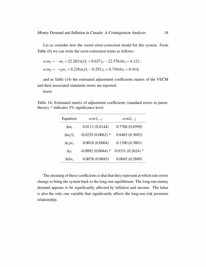
Let us consider now the vector error-correction model for this system. FromTable (6) we can write the error-correction terms as follows:

ecm1 =�mt +22.283 in f lt +0.627yt �22.576 tbrt +4.121;

ecm2 =�cprt +0.238 in f lt �0.292yt +0.710 tbrt +0.414;

and in Table (14) the estimated adjustment coefficients matrix of the VECMand their associated standards errors are reported.

know

Table 14: Estimated matrix of adjustment coefficients (standard errors in paren-theses), * indicates 5% significance level.

Equation ecm1t�1 ecm2t�2

Dmt 0.0111 (0.0144) 0.7768 (0.8599)

Din f lt -0.0229 (0.0062) * 0.6465 (0.3692)

Dcprt 0.0018 (0.0064) 0.1390 (0.3801)

Dyt -0.0092 (0.0044) * 0.9331 (0.2624) *

Dtbrt 0.0078 (0.0045) 0.0045 (0.2689)

The meaning of these coefficients is that that they represent at which rate errorschange to bring the system back to the long-run equilibrium. The long-run moneydemand appears to be significantly affected by inflation and income. The latteris also the only one variable that significantly affects the long-run risk premiumrelationship.


Conclusions

The objective of this empirical work has been to investigate the presence of coin-tegrating relationships among the variables that explain Canadian money demand.The reason of doing this is that cointegration in multivariate time series mod-els may bring significant improvements in forecasting, as their analysis allowthe researcher to discover relations with stationary properties as a result of non-stationary time series interactions.

The analysis have been carried out on quarterly data covering a time rangegoing from June 1983:2 to March 2011:2. The first step of these analysis wasto identify the optimal lag p in order to determine the number r of cointegratingrelationships involved in the variables, determining p = 4 and r = 2. With thesevalues, I have estimated the model setting some theoretical assumptions usefulto express a theoretical (and a priori) relation for money demand, inflation andrisk premium. This (unconstrained) model has been considered as a benchmarkagainst which other models –constrained on purpose by means of different restric-tions imposed on coefficients in some variables. The results obtained by meansof maximum likelihood estimation have shown that no constrained model is bet-ter then the unconstrained one. Therefore, I considered the unconstrained modeland evaluated its goodness by means of normality tests, a white noise test, a La-grange Multipliers and a serial correlation test performed on residuals. Resultshave shown that residuals are not significantly different from a white noise pro-cess. However, the null hypothesis of normally distributed residuals is rejected.These results invalidate the power of the model in describing the system.

Finally, the sensitivity tests have shown that the long-run money demand issignificantly affected both by inflation and income, while the risk-premium rela-tionship is affected only by income.


References

[1] Ball, L., 2001, Another Look at Long–Run Money Demand, Journal of Mon-etary Economics 47, 31-44.

[2] Granger, C. W. J. and Newbold, P. (1974), Spurious regressions in economet-rics. Journal of Econometrics 2 (2): 111–120.

[3] Granger, Clive (1981), Some Properties of Time Series Data and Their Use inEconometric Model Specification. Journal of Econometrics 16 (1): 121–130.

[4] Engle, Robert F.; Granger, Clive W. J. (1987). Co-integration and error correc-tion: Representation, estimation and testing. Econometrica 55 (2): 251–276.

[5] Lucas, R. E., 1988, Money Demand in the United States: A QuantitativeReview, Carnegie Rochester Conference Series on Public Policy 29, 137–168.

[6] Meltzer, A. H., 1963, The Demand for Money: Evidence from Time Series,Journal of Political Economy 71, 219–246

[7] Verbeek, M. (2009). A guide to modern econometrics. J. Wiley & Sons press.

Documents

Munich Personal RePEc Archive - uni-muenchen.de · 0 3 5 $ Munich Personal RePEc Archive Money Demand and In ation: A Cointegration Analysis for Canada Federico Lubello Department