UNITED STATES ENVIRONMENTAL PROTECTION AGENCY WASHINGTON D.C. 20460

OFFICE OF THE ADMINISTRATORSCIENCE ADVISORY BOARD

September 28, 2017

EPA-CASAC-17-004

The Honorable E. Scott PruittAdministratorU.S. Environmental Protection Agency1200 Pennsylvania Avenue, N.W.Washington, D.C. 20460

Subject: CASAC Review of the EPA’s Integrated Science Assessment for Oxides of Nitrogen, Oxides of Sulfur, and Particulate Matter – Ecological Criteria (First External Review Draft – February 2017)

Dear Administrator Pruitt:

The Clean Air Scientific Advisory Committee (CASAC) Secondary NAAQS Review Panel for Oxides of Nitrogen and Sulfur met on May 24-25, 2017, and August 31, 2017, to peer review the EPA’s Integrated Science Assessment for Oxides of Nitrogen, Oxides of Sulfur, and Particulate Matter – Ecological Criteria (First External Review Draft), hereafter referred to as the Draft ISA. The Chartered CASAC approved the Panel’s report on August 31, 2017. The CASAC’s consensus responses to the agency’s charge questions and the individual review comments from the Panel are enclosed.

Overall, the CASAC finds the Draft ISA to be a remarkably comprehensive and well done assessment of the science characterizing the ecological effects caused by oxides of nitrogen, oxides of sulfur, and particulate matter. This is a broad and complex subject and the EPA is to be commended for the quality of the work represented by this Draft ISA. The CASAC provides recommendations to further enhance the rigor of the assessment and strengthen the organization and presentation of the material in the document.

The CASAC recommends that the length of the Draft ISA be reduced by moving some material into appendices, and that the EPA consider including an integrative or shorter overview section in the Executive Summary. The CASAC suggests that additional references listed in the enclosed report be included in the final ISA, and that there be stronger cross-referencing among chapters on key topics. The following summarizes chapter highlights from the CASAC’s review of the Draft ISA, with detailed comments in the enclosed report.

The Draft ISA Executive Summary is an effective synopsis, and Chapter 1 is a good synthesis of the findings presented in the document. The EPA has appropriately applied and presented the causality framework in Chapter 1 and the Executive Summary. The CASAC recommends that the following topics be discussed in Chapter 1: (1) key scientific uncertainties; (2) components of National Ambient Air Quality Standards (NAAQS); (3) science not reviewed in the Draft ISA because it will be addressed in the policy-oriented phase of the NAAQS review; (4) the Aquatic Acidification Index (AAI) developed as part of the previous NAAQS review for oxides of nitrogen and sulfur; (5) the concept of critical loads (including the strengths and limitations of approaches to developing and implementing critical loads); (6) key conceptual changes in the science since the last review; and (7) an overview of important concepts and linkages on these topics across different parts of the document.

Chapter 2 of the Draft ISA presents an accurate and comprehensive picture of the fundamentals of emissions, atmospheric chemistry, transport, and deposition of the major nitrogen and sulfur species. The CASAC recommends that in Chapter 2, and throughout the Draft ISA, quantitative estimates or indications of the relative magnitude of uncertainties be provided. In addition, the CASAC recommends that: (1) a comprehensive discussion of the major atmospheric transport and flux modeling platforms be included in Chapter 2; (2) the process used to obtain emissions estimates (including estimates of ammonia emissions) in Chapter 2 be better documented; (3) text be added to Chapter 2 to discuss the usefulness of data from various monitoring networks to estimate deposition; and (4) more definitive conclusions be presented about the usefulness of transference ratios for linking ambient air quality to total deposition.

Chapter 3 of the Draft ISA is a well-written assessment of the science concerning gas-phase effects of oxides of sulfur and oxides of nitrogen on vegetation. The CASAC notes that the ecological effects of reduced nitrogen compounds are important for understanding the effects of total reactive atmospheric nitrogen deposition and should be included in Chapter 3 and other chapters of the Draft ISA. Ammonia emissions are increasing in many regions of the U.S. and the CASAC recommends that EPA consider the need for developing National Ambient Air Quality Standards that encompass reduced forms of nitrogen during the Risk and Exposure Assessment and Policy Analysis phases of this NAAQS review.

Chapter 4 of the Draft ISA summarizes soil biogeochemical responses to atmospheric sulfur and nitrogen deposition. The chapter is generally complete with respect to the discussion of indicators, processes, models, monitoring, and sensitivity across the U.S. The CASAC recommends that front materials be included in Chapter 4 (and other ecological effects chapters in the Draft ISA) to discuss cross-cutting issues. In addition, the CASAC recommends that Chapter 4 contain more discussion of the relevant critical mechanisms that control dissolved organic carbon release, decomposition, and changes in belowground carbon pools and fluxes. It would also be useful to present maps in Chapter 4 to show the relative contribution of sulfate, oxidized nitrogen, and reduced nitrogen driving acidification and eutrophication effects, particularly for areas of the U.S. where acidification and nitrogen critical loads are exceeded.

Chapter 5 of the Draft ISA is a well-organized and well-written assessment of the effects of acidification on terrestrial biota. The CASAC finds that Chapter 5 has important linkages to topics discussed in Chapters 4 and 6 and recommends that these chapters be cross-referenced. In

addition, the CASAC finds that much of the literature reviewed in Chapter 5 concerns natural variability in soil pH, calcium concentration, and base saturation impacts on plant health and microbial composition (rather than effects of nitrogen or sulfur deposition on acidification). These studies are useful for understanding basic physiological principles of acidification effects on biota, but the Draft ISA should clearly identify studies that are not based on elevated levels of nitrogen or sulfur deposition. This chapter should emphasize studies with nitrogen and sulfur deposition linkages.

Chapter 6 of the Draft ISA is a comprehensive assessment of the effects of excess nitrogen on the structure and function of terrestrial ecosystems. To a great extent, Chapters 5 and 6 of the Draft ISA are paired in scope. The CASAC recommends that the EPA provide stronger linkages between Chapters 4, 5, and 6 to reduce redundancy and make the document easier to read. The CASAC also suggests that Chapter 6 contain an upfront summary and concise conclusions, and recommends that the chapter contain additional information on the effects of nitrogen on bacteria and archaea.

Chapter 7 of the Draft ISA is a good synthesis and summary of a large body of literature on the biogeochemical response of freshwater and estuarine systems to nitrogen and sulfur deposition. In Chapter 7, freshwater eutrophication is discussed in far greater detail than estuarine eutrophication, and the review of acidification is more detailed and comprehensive than the review of nitrogen effects. The CASAC recommends that estuarine indicators of eutrophication, estuarine monitoring, and water quality criteria for estuaries be given greater attention in this chapter. The CASAC also recommends that a framework be provided in Chapters 4, 5, 7, and 8 to define ecological recovery, and suggests that the section on dissolved organic carbon be rewritten to address specific concerns identified in the enclosed report.

Chapter 8 of the Draft ISA is a comprehensive synthesis of the scientific knowledge of biological indicators of acidifying deposition and effects on biodiversity of freshwater biota. The CASAC recommends that Section 8.4.6 of the chapter discuss the different mitigation responses of direct application of lime on water and whole watershed liming. The CASAC also recommends that parts of the text in Chapters 7 and 8 be cross-referenced to minimize redundancy. In addition, the CASAC recommends that in Chapter 8 a clearer distinction be made between controls on biological responses in glaciated versus unglaciated regions.

Chapter 9 of the Draft ISA is a concise, up-to-date synthesis of the scientific literature on biological effects of nitrogen deposition to freshwater systems. The chapter reflects increasing recognition that nitrogen plays an important role as a limiting nutrient in many freshwater systems. The CASAC notes that atmospheric phosphorus deposition may also affect nitrogen and phosphorus nutrient limitations and recommends that a discussion of atmospheric phosphorus deposition be included in Chapter 9.

Chapter 10 of the Draft ISA is a thorough and well-documented synthesis of the literature on biological indicators and effects of nitrogen enrichment in coastal areas. The CASAC notes that reduced forms of atmospheric nitrogen play an increasingly important role in estuarine and coastal eutrophication, and in harmful algal bloom dynamics. Therefore, the ecological impacts of reduced forms of N should receive more attention in Chapter 10. The chapter should also

indicate that acidification of estuaries is driven by decomposition of organic matter from changing land use, erosion and deforestation as well as respiration of living algae and seagrasses.

Chapter 11 of the Draft ISA synthesizes and summarizes the recent literature on the effects of excess nitrogen on a wide variety of wetland ecosystems. The CASAC finds that Chapter 11 is a thorough review of the current biogeochemical and ecological literature on this topic.

Chapter 12 of the Draft ISA presents a detailed overview of the effects of sulfur enrichment in freshwater aquatic and wetland ecosystems. The CASAC recommends that a better synthesis be developed, which articulates the multiple cause and effect chains that determine the effects of sulfate inputs on methyl mercury production and bioaccumulation.

Chapter 13 of the Draft ISA addresses climate modification of ecosystem responses to nitrogen and sulfur deposition. The chapter should indicate that the changing character of atmospheric temperatures, precipitation, and increasing carbon dioxide levels can modify processes discussed in the other chapters (Chapters 3 to 12) of the ISA. Cross-referencing should be improved to more clearly illustrate connections to the other chapters. The CASAC recommends that the EPA also integrate climate change effects into each of the effects chapters of the Draft ISA. By including only a separate chapter on climate change at the end of the document, the EPA may convey the incorrect message that this is a minor issue to be considered in the NAAQS review.

Chapter 14 of the Draft ISA discusses recent advances in the science of ecosystem services analysis. Recommendations to improve Chapter 14 include: (1) incorporating a better definition of ecosystem services; (2) explaining why ecosystem services analysis is important; (3) incorporating “plain spoken” stories or narratives to help the public understand aspects of human welfare that are affected by emissions of oxides of nitrogen, oxides of sulfur, and particulate matter; (4) incorporating a clear statement of conclusions; and (5) incorporating a summary table in the Draft ISA to list ecosystem services in the U.S. that are potentially affected by oxides of nitrogen, oxides of sulfur, and particulate matter.

Appendix C of the Draft ISA describes place based case-studies at five locations. Appendix D of the document describes the ecological effects of particulate matter components other than nitrogen and sulfur. The information in the five case studies is clearly presented and relevant. However, the CASAC recommends that an additional case study on the Adirondacks ecosystem be included in the Appendix. This ecosystem has been significantly impacted by nitrogen and sulfur deposition over a long period of time and it is one of the most extensively studied ecosystems in the U.S. The CASAC finds that Appendix D is a well-written summary of current research on the direct and indirect ecological effects of non-nitrogen and non-sulfur particles. The information in Appendix D provides a useful update on this topic.

The CASAC appreciates the opportunity to provide advice on the Draft ISA for Oxides of Nitrogen, Oxides of Sulfur, and Particulate Matter and looks forward to reviewing the second draft of the document.

Sincerely,

/s/ /s/

Dr. Ana Diez Roux, Chair Dr. Ivan J. Fernandez, ChairClean Air Scientific Advisory Committee CASAC Secondary NAAQS Review

Panel for Oxides of Nitrogen and Sulfur

Enclosure

NOTICE

This report has been written as part of the activities of the EPA's Clean Air Scientific Advisory Committee (CASAC), a federal advisory committee independently chartered to provide extramural scientific information and advice to the Administrator and other officials of the EPA. The CASAC provides balanced, expert assessment of scientific matters related to issues and problems facing the agency. This report has not been reviewed for approval by the agency and, hence, the contents of this report do not represent the views and policies of the EPA, nor of other agencies within the Executive Branch of the federal government. In addition, any mention of trade names or commercial products does not constitute a recommendation for use. The CASAC reports are posted on the EPA website at: http://www.epa.gov/casac.

i

U.S. Environmental Protection AgencyClean Air Scientific Advisory Committee

Secondary NAAQS Review Panel for Oxides of Nitrogen and Sulfur

CHAIRDr. Ivan J. Fernandez, Distinguished Maine Professor, School of Forest Resources and Climate Change Institute, University of Maine, Orono, ME

MEMBERSDr. Edith Allen, Professor of Plant Ecology, Department of Botany and Plant Sciences, University of California Riverside, Riverside, CA

Dr. Praveen K. Amar, Independent Consultant, Environment, Energy, and Climate Strategies, Lexington, MA

Dr. James Boyd, Senior Fellow and Director, Center for the Management of Ecological Wealth, Resources for the Future, Washington, DC

Dr. Elizabeth W. Boyer, Associate Professor of Water Resources, Department of Ecosystem Science and Management, Pennsylvania State University, University Park, PA

Dr. Douglas Burns, Research Hydrologist, New York Water Science Center, U.S. Geological Survey, Troy, NY

Ms. Lauraine Chestnut, Independent Consultant, Denver, CO

Dr. Charles T. Driscoll, Jr., Distinguished Professor and University Professor of Environmental Systems Engineering, Department of Civil and Environmental Engineering, College of Engineering and Computer Science, Syracuse University, Syracuse, NY

Dr. Mark Fenn, Research Plant Pathologist, Pacific Southwest Research Station, USDA Forest Service, Riverside, CA

Dr. James Galloway, Sidman P. Poole Professor of Environmental Sciences, Department of Environmental Sciences, University of Virginia, Charlottesville, VA

Dr. Frank Gilliam, Professor, Department of Biological Sciences, Marshall University, Huntington, WV

Dr. Robert A. Goldstein*, Senior Technical Executive for Water and Ecosystems, Electric Power Research Institute, Palo Alto, CA

Dr. Daven Henze, Associate Professor and Johnson Faculty Fellow, Department of Mechanical Engineering, University of Colorado, Boulder, CO*Not participating in this review.

ii

*Not participating in this review.iii

Dr. Robert W. Howarth, David R. Atkinson Professor of Ecology & Environmental Biology, Department of Ecology and Evolutionary Biology, Cornell University, Ithaca, NY

Dr. Donna Kenski, Data Analysis Director, Lake Michigan Air Directors Consortium, Rosemont, IL

Dr. William McDowell, Professor of Environmental Science, Department of Natural Resources and the Environment, University of New Hampshire, Durham, NH

Dr. Erik Nelson, Assistant Professor, Department of Economics, Bowdoin College, Brunswick, ME

Dr. Hans Paerl, Kenan Professor of Marine and Environmental Sciences, Institute of Marine Sciences, University of North Carolina - Chapel Hill, Morehead City, NC

Mr. Richard L. Poirot, Independent Consultant, Burlington, VT

Dr. Armistead (Ted) Russell, Howard T. Tellepsen Chair and Regents Professor of Civil and Environmental Engineering, Department of Civil and Environmental Engineering, Georgia Institute of Technology, Atlanta, GA

Dr. Stephen E. Schwartz, Senior Scientist, Environmental and Climate Sciences Department, Brookhaven National Laboratory, Upton, NY

Dr. Kathleen Weathers, Senior Scientist, Cary Institute of Ecosystem Studies, Millbrook, NY

SCIENCE ADVISORY BOARD STAFFDr. Thomas Armitage, Designated Federal Officer, U.S. Environmental Protection Agency, Science Advisory Board, Washington, DC

iv

U.S. Environmental Protection AgencyClean Air Scientific Advisory Committee

CHAIRDr. Ana V. Diez Roux, Dean, School of Public Health, Drexel University, Philadelphia, PA

MEMBERSDr. Judith Chow, Nazir and Mary Ansari Chair in Entrepreneurialism and Science and Research Professor, Division of Atmospheric Sciences, Desert Research Institute, Reno, NV

Dr. Ivan J. Fernandez, Distinguished Maine Professor, School of Forest Resources and Climate Change Institute, University of Maine, Orono, ME

Dr. Jack Harkema, Distinguished University Professor, Department of Pathobiology and Diagnostic Investigation, College of Veterinary Medicine, Michigan State University, East Lansing, MI

Dr. Donna Kenski, Data Analysis Director, Lake Michigan Air Directors Consortium, Rosemont, IL

Dr. Elizabeth A. (Lianne) Sheppard, Professor of Biostatistics and Professor and Assistant Chair of Environmental & Occupational Health Sciences, School of Public Health, University of Washington, Seattle, WA

Dr. Ronald Wyzga, Technical Executive, Air Quality Health and Risk, Electric Power Research Institute, Palo Alto, CA

SCIENCE ADVISORY BOARD STAFFMr. Aaron Yeow, Designated Federal Officer, U.S. Environmental Protection Agency, Science Advisory Board, Washington, DC

v

Consensus Responses to Charge Questions on EPA’s Integrated Science Assessment for Oxides of Nitrogen, Oxides of Sulfur, and

Particulate Matter – Ecological Criteria (First External Review Draft – February 2017)

As part of the ongoing review of the secondary (welfare-based) national ambient air quality standards (NAAQS) for Oxides of Nitrogen (NOX), Oxides of Sulfur, and Particulate Matter, EPA’s National Center for Environmental Assessment prepared a draft document titled Integrated Science Assessment for Oxides of Nitrogen, Oxides of Sulfur, and Particulate Matter – Ecological Criteria (Draft ISA). The Clean Air Scientific Advisory Committee (CASAC) Secondary NAAQS Review Panel for Oxides of Nitrogen and Sulfur reviewed EPA’s Draft ISA. Panel members provided individual comments prior to a public meeting held on May 24-25, 2017. At the meeting the Panel received a briefing on the Draft ISA, heard public comments, and deliberated on responses to the EPA’s charge questions. Draft consensus responses to the charge questions were developed by Panel subgroups based on the deliberation. At a teleconference meeting held on August 31, 2017, the Panel discussed its consensus responses and the Chartered CASAC conducted a quality review and approved the Panel’s report.

The introductory text in the Draft ISA states that the document is intended to provide a comprehensive evaluation and synthesis of the most policy-relevant science aimed at characterizing the ecological effects caused by oxides of nitrogen, oxides of sulfur, and particulate matter (PM). The Draft ISA indicates that these criteria pollutants have been reviewed together because they all contribute to nitrogen (N) and sulfur (S) deposition, which causes substantial ecological effects.

The term “oxides of nitrogen” is defined in the Draft ISA as total oxidized N, including nitrate (NO3−),

nitric oxide (NO) and nitrogen dioxide (NO2), and all other oxidized N containing compounds formed from NO and NO2. Oxides of sulfur (SOX) are defined to include sulfur monoxide (SO), sulfur dioxide (SO2), sulfur trioxide (SO3), disulfur monoxide (S2O), and sulfate (SO4

2−). It is noted in the Draft ISA that SO, SO3, and S2O are not discussed because they occur at much lower ambient levels than SO2 and SO4

2–. The Draft ISA further indicates that particulate matter is composed of some or all of the following components: NO3

−, SO42−, ammonium (NH4

+), metals, minerals (dust), and organic and inorganic carbon.

The EPA’s charge questions to the CASAC with a summary response to each are presented below. Other comments and technical corrections are included in Appendix A of this report, and the individual comments of members of the CASAC Secondary NAAQS Review Panel for Oxides of Nitrogen and Sulfur are included in Appendix B of this report.

Executive Summary and Chapter 1

Charge Question #1. The Executive Summary and Chapter 1 provide overviews of the ISA. The Executive Summary is intended to be a concise synopsis of key findings targeted to a broad audience, whereas Chapter 1 is a more detailed synthesis of the ISA’s most policy-relevant findings.

a. Please comment on the extent to which the Executive Summary and Chapter 1 meet their objectives.

b. The causality determinations are summarized in the Executive Summary and Chapter 1, please comment on the extent to which the causal framework is appropriately applied to evidence for each of the effect categories in chapters 3-12 to form causal determinations.

1

General Comments on the Executive Summary and Chapter 1

The CASAC provides the following general comments on the Executive Summary and Chapter 1 of the ISA.

The Draft ISA and its Executive Summary are lengthy (1,412 pages). The CASAC finds that reducing the length of the Draft ISA and Executive Summary would make the document more accessible. In this regard, the CASAC recommends that the EPA consider presenting more of the material in appendices to the Draft ISA.

The topic of uncertainty is particularly important and should be addressed in greater detail in the Draft ISA. The CASAC notes that uncertainty was a key factor considered in the last review of the secondary NAAQS for oxides of N and S.0F

1 Therefore, the CASAC recommends that uncertainty be addressed in each chapter of the Draft ISA and collectively in the integrated summary of the Draft ISA, with a focus on the most important uncertainties in the literature, and how they should be treated from a scientific perspective to inform policy determinations.

Some of the CASAC’s comments on the ISA focus on issues that may be addressed in later, policy-oriented phases of the review of the secondary NAAQS for oxides of N, oxides of S, and particulate matter. The CASAC recommends that the scientific aspects of these comments, however, be addressed in the Draft ISA. In particular, the scientific aspects of specific models and approaches that will be used in analyses to develop the Risk and Exposure Assessment (REA) and Policy Assessment (PA) should be reviewed in the Draft ISA. The detailed information could be provided in appendices to the document. The CASAC also recommends that the EPA clearly identify science topics that are not thoroughly reviewed in the ISA because they are to be addressed in the policy-oriented phase of the review. The EPA should also explain why these topics are best addressed in the policy phase of the review.

Key Findings in Response to Charge Question 1

The CASAC finds that the Executive Summary of the Draft ISA is an effective synopsis of the rest of the document, although it is lengthy for an Executive Summary, reflecting the document as a whole in that regard. As opportunities to reduce the length of the Draft ISA are realized, they should be reflected in the Executive Summary. Given the length of the Executive Summary, a final, integrative section (or possibly a shorter overview of the Executive Summary on the order of five pages) should be included. The CASAC also recommends that the Executive Summary integrate the most informative figures from the chapters of the Draft ISA, as well as the table of causal determinations that was included in EPA’s presentation at the CASAC Panel meeting on May 24-25, 2017.

Chapter 1 of the Draft ISA is both an introduction and an integrated synthesis. The CASAC finds that Chapter 1 provides a good synthesis of the rest of the Draft ISA, although the inclusion of more introductory material in the chapter is warranted. Consideration should be given to presenting the introduction and integrative synthesis in separate chapters. The CASAC recommends that the following

1 The Administrator’s decision in the last review cycle was that, while the secondary standards were inadequate to protect against adverse effects from deposition of oxides of nitrogen and sulfur, it was not appropriate to set any new secondary standards at that time due to the limitations in the available data and uncertainty as to the amount of protection the metric developed in the review would provide against acidification effects across the country (77 FR 20218).

2

topics be more comprehensively covered in the introduction. Detailed information could be provided in an appendix, with some text included in the introduction to encapsulate the main points.

A presentation of the NAAQS associated with this review, the requirements/components of the NAAQS (form, indicators, level, averaging time), and a discussion of how these requirements/components may impact the formulation of a standard should be included in the introduction. The discussion should address how requirements of the NAAQS impact aspects of an integrated scientific assessment (e.g., how an ambient concentration may be related to a metric of deposition or ecological impact, the need to have a national, not regional, standard, etc.) While some of these topics are a matter of policy, they have ramifications with regard to the scientific concepts that may be applied to inform the setting of a NAAQS.

The Aquatic Acidification Index (AAI) developed as part of the last NAAQS review for oxides of N and S should be discussed in the introduction. This discussion should reflect the points mentioned above (i.e., the points covered in the discussion of the NAAQS). The discussion should also address the uncertainties identified in the last review (e.g., uncertainties in the Risk and Exposure Assessment and Policy Assessment, as well as the uncertainties considered in the Administrator’s decision).

A new section should be included near the beginning of Chapter 1 on uncertainties. Further, the CASAC suggests that a section on “Concepts, Connections, and Changes” be added. This second section could provide readers with a clearer view of: what is to be presented (e.g., important concepts such as deposition, critical load, and biodiversity); major conceptual changes in the science since the last review (i.e., Changes); how different aspects of the Draft ISA fit together (i.e., Connections); and specific aspects of the review of the science that might be most informative (i.e., Changes and Concepts). The integrated synthesis should focus on, and specifically identify, “what matters.”

The CASAC recommends that the concept of critical load be more clearly discussed in the introduction and integrated synthesis. In this regard, it is important to differentiate between what may be called a “scientist’s critical load” and a “policy-maker’s critical load.” The former is the traditional critical load which has been defined (Nilsson and Grennfeld 1988) as: “The quantitative estimate of an exposure to one or more pollutants below which significant harmful effects on specified sensitive elements of the environment do not occur according to present knowledge.” The policy-maker’s critical load has also been referred to as a “target load.” Fenn et al (2011) have defined the target load as follows: “The acceptable pollution load that is agreed upon by policy makers or land managers. The target load is set below the critical load to provide a reasonable margin of safety, but could be set higher than the critical load at least temporarily.” Target loads (policy thresholds) are selected based on the level of ecosystem protection desired, economic considerations, and stakeholder input at a given location. In discussing the concept of critical load it is also important to discuss the degree to which a critical load is a line or inflection point, and to address the gradient of effects. In addition, the CASAC recommends that the discussion of critical load indicate that critical loads may vary in time due to past cumulative deposition. It is important to explain what historically large deposition fluxes mean with regard to increased or decreased susceptibility.

Although the CASAC finds that the Executive Summary is a good summary of the Draft ISA, modifications to Chapter 1 (and other chapters) should be reflected in a revised Executive Summary. In particular, this would apply to the expanded scientific assessment of the approaches used in the prior review and the section on “Concepts, Connections, and Changes.”

3

The CASAC was also asked to comment on the extent to which the causal framework (summarized in the Executive Summary and Chapter 1) is appropriately applied to evidence for each of the effect categories in Chapters 3-12 to form causal determinations. The CASAC finds that the causality framework was appropriately applied and well presented in the Draft ISA. The CASAC recommends, however, that the table of causal determinations included in EPA’s presentation at the CASAC Panel meeting on May 24-25, 2017, also be included in the Draft ISA. In addition, the CASAC recommends expanding the text on the relationship of causal findings to past, current, and future conditions.

Atmospheric Chemistry of Nitrogen and Sulfur Species (Chapter 2)

Charge Question 2. Chapter 2 describes scientific information on sources, atmospheric chemistry, measurement, modeling, ambient concentration trends, and atmospheric deposition of oxides of sulfur and nitrogen and suspended particulate matter.

a. Please comment on the accuracy, clarity, level of detail, and relevance of the information presented regarding sources, chemistry, and measurement and modeling of ambient concentrations.

b. Please comment on the accuracy, clarity, level of detail, and relevance of the information presented regarding measurement, modeling, prediction, and trends of atmospheric deposition of nitrogen and sulfur, including particulates, and related processes.

General Comments on Chapter 2

In Chapter 2, and throughout the entire Draft ISA, uncertainty is mentioned frequently but often qualitatively and seldom in a systematic fashion. As previously noted, a greater discussion of uncertainty in this ISA is necessary. Every effort should be made to provide quantitative estimates or indications of the relative magnitude of uncertainties and associated confidence, perhaps following the example of the Intergovernmental Panel on Climate Change (IPCC 2017) which has adopted a formal nomenclature ("likely," "highly likely," etc.) corresponding to specific likelihoods that the actual value of a quantity is within a specified likelihood range. Structural uncertainty (e.g., arising from the use of transference ratios) should be distinguished from quantitative uncertainty (e.g., associated with measurements of concentration and deposition or with estimates of emission rates). Policy makers must understand what uncertainty means and how it is used as input to decision making.

The precision with which quantities are expressed (and the resultant implied uncertainty) is closely related to uncertainty. For example, Table 2-1 in the Draft ISA presents emissions of several species by process, often to two significant figures (e.g., 0.74 for NOx by off-highway vehicles). This implies rather precise knowledge of the quantity, which seems highly optimistic. It seems essential that such tables include estimates of uncertainty with clearly stated meaning of the uncertainty range.

Key Findings in Response to Charge Question 2

The CASAC commends the EPA for its excellent and thorough work to develop Chapter 2 of the Draft ISA. In large part, the EPA has succeeded in accurately and clearly presenting a comprehensive description of the fundamentals of emissions, atmospheric chemistry, transport, and deposition of the major N and S species; the CASAC recognizes that developing this chapter was a monumental undertaking. The following recommendations and suggestions are offered to improve the organization and presentation of this material.

4

Structural changes: The CASAC suggests that the EPA move the summary (now Section 2.11) to the front of Chapter 2 and organize the rest of the chapter around the summary (just as the ISA itself begins with a summary). This approach will convey to the reader the major points discussed, provide structure and context, and set the stage for the expanded discussions on each topic that follows.

Modeling: The CASAC finds that a comprehensive discussion of the major modeling platforms, (particularly their role in generating metrics being considered for quantifying ecological and welfare impacts, and their role in evaluating the relationship between these metrics, emissions, and ambient concentrations) is missing from Chapter 2. In particular, Sections 2.4 (Atmospheric Transport) and 2.7.2 (Dry Deposition Flux) seem either too detailed or incomplete, or out of place in their current positions. The CASAC recommends that: (1) a new section be added to Chapter 2 to provide an overview of the chemical transport models, and (2) shorter or more directed versions of the transport and flux discussions be incorporated into the modeling discussion. Any data comparing model performance, especially of hybrid satellite/chemistry transport models (CTMs), would be particularly useful. Source-receptor relationships should also be addressed more quantitatively and accompanying uncertainty information should be provided.

The CASAC notes that not all species of N deposited from the atmosphere are routinely monitored, and the monitoring network for both oxidized N and S species is sparse. Further, wet deposition is also sparsely measured, and dry deposition is mostly modeled. These points should be taken into account when considering the potential use of models in the attainment decision process for secondary standards. The use of models in the attainment process should be based on science, and an assessment of the accuracy of models used for such a purpose should be provided.

Emissions: The emissions data presented in Chapter 2, especially emissions of ammonia (NH3), are somewhat superficial. The process used to obtain the emissions estimates in Table 2.1 needs better documentation. Data sources and associated uncertainties should be identified. The role of soil NOx should be discussed. It is not clear whether this is included in biogenic emissions or agriculture. It should be noted that the role of agricultural sources dominates Continental United States (CONUS) NHx emissions (Xing et al. 2013), but the transport sector can be an important source of NHx emissions for ecological effects downwind of urban centers or highly traveled road networks (Weiss 1999; Bettez et al. 2013). This suggests that evaluations of the relative importance of the agricultural and transport sector contributions to ammonia emissions should be region-specific.

Monitoring networks: The CASAC finds that the measurement discussion in Section 2.5 is not entirely clear with regard to why the data from various networks are useful, or not, for determining deposition. It is also not clear why some types of measurements are discussed in this section but others are not (i.e., NH3 mobile and aircraft observations, or remote sensing of NH3 from the Atmospheric Infrared Sounder [AIRs] and Cross-Track Infrared Sounder [CrIS]). The CASAC notes that data from monitoring networks are crucial to estimating deposition and secondary effects. Section 2.5 should contain a more straightforward discussion of the inadequacy of the NO2 federal reference method (FRM) for determining ecological effects of N. The CASAC also notes the overwhelming dependence of the advancement of science on the National Atmospheric Deposition Program (NADP) and Clean Air Status and Trends Network (CASTNET) data. These networks are critically important to advancing science as well as documenting long-term trends in air quality. Figure 2-27 (documenting changes in the pH of precipitation over the continental U.S. between two periods, 1989 to 1991 and 2011 to 2013) is an astonishing tribute to the effectiveness of the Clean Air Act Amendments, and should be an icon to the effectiveness of this legislation and to EPA. The

5

CASAC recommends that this be explicitly noted. The CASAC is concerned that the NADP and CASTNET are funded by multiple agencies and organizations and lack long-term, stable funding commitments. The CASAC also suggests that the EPA include in the Draft ISA (rather than later in the review process) an assessment of the adequacy of the existing networks to support the current review. Notwithstanding the accomplishments of NADP and CASTNET, the EPA should also discuss the limitations of these networks to support the current review of secondary effects, particularly for more polluted sites, and/or the evaluation of various secondary NAAQS that may be considered.

Transference ratios: Transference ratio is a relatively new concept that was discussed in the Policy Assessment during the last review of the NAAQS. The concept is an interesting addition to the literature, but it leaves many questions unanswered. Section 2.9 does not come to a definitive conclusion concerning transference ratios, except to say “there is uncertainty.” This chapter should discuss the point that there is a mass balance in the atmosphere, and reactive N and S emissions have limited lifetimes in the atmosphere, thus a decrease in the transference ratio does not lead to a similar decrease in the flux of a particular species from atmosphere to land.1F

2 The issue of lifetimes and the relationship of lifetime to transference ratios should also be further discussed in Chapter 2.

Bidirectional exchange: In Chapter 2 of the Draft ISA there are strong statements about the importance of bidirectional exchange. However, no results are shown to indicate how bidirectional exchange impacts model estimates of concentrations or deposition, or more broadly, the ecosystems of concern. It is unclear when and where consideration of bidirectional exchange is important. The importance of bidirectional exchange should be explicitly addressed in Chapter 2 and additional references should be included.

Deposition and Critical Loads: In the Draft ISA there is considerable discussion of critical loads, but in the section on the distributions and trends in actual deposition values, the trends are presented with little reference to their magnitudes in comparison to the relevant critical loads. Recent research, e.g., Ellis et al. (2013) and Lee et al. (2016) as well as others, that broadly examines drivers of deposition above critical loads, should be discussed in the ISA.

Maps: The Schwede and Lear (2014) maps as well as the global-scale, three-dimensional, chemistry-transport model (GEOS-Chem) and Community Multiscale Air Quality modeling system (CMAQ) maps in the Draft ISA are visually appealing and informative, despite sub-optimal color scales in some cases. The detailed format, however, implies more certainty than is actually there, so it is important to address this uncertainty directly. The method used also fails to maintain mass balance and this should be noted. The CASAC proposes including a set of linked maps of the emissions fluxes (in mass per area per time), atmospheric concentrations (in mass per volume), and deposition (in mass per area per time) as a theme. Such a set of maps could effectively illustrate key points in the chapter, linking emissions, chemistry, transport, lifetime, and deposition. Consideration should be given to moving much of the detailed information in this chapter into an appendix. 

Background: More information on background concentrations and deposition should be included in Chapter 2; for example, see Galloway et al. (1982), and NADP data from remote sites such as Alaska could be included.

2 In this instance, reactive N is defined as all N species that have residence times of less than one month in the atmosphere. For example, NO, NO2, HNO3, and nitrate aerosol would be included, but N2O would not.

6

Effects of Gas-Phase SO2, NO2, NOx, PAN, and HNO on Vegetation (Chapter 3)

Charge Question 3. Chapter 3 characterizes scientific evidence on the effects of gas-phase SO2, NO2, NO, peroxyacetyl nitrate (PAN), and HNO3 on vegetation. Please comment on the characterization of these effects and the integration of new information into the long history of evidence on this topic.

General Comments on Chapter 3

The CASAC notes that the effects of SO2-NOx on vegetation and ecosystems are intimately connected to ammonia and ammonium (NHx). NH3 emissions in many regions of the U.S. are increasing (Li et al. 2016). Ecological impacts of reduced N on vegetation and ecosystems are critical to an overall understanding of effects of atmospheric N deposition since N is delivered to ecosystems in both NOx and NHx forms. Impacts of NHx range from effects on plant physiology and plant productivity, to ecosystem acidity and nutrient cycling. The importance of NH3 emissions, NHx deposition, and secondary effects of NHx should be emphasized throughout the Draft ISA. The CASAC recommends that the EPA consider the need for developing National Ambient Air Quality Standards that encompass reduced forms of nitrogen during the Risk and Exposure Assessment and Policy Analysis phases of this NAAQS review.

Key Findings in Response to Charge Question 3

The CASAC provides the following key findings in response to Charge Question 3.

Chapter 3 of the Draft ISA is well-written. The important points in the chapter are clearly articulated. Text should be included in Chapter 2 and/or Chapter 3 to clearly discuss the relationship between the

standard for NO2 and other forms of oxidized N.

Other chapters of the Draft ISA contain maps of the U.S. showing current SO2, NOx and nitric acid by region as well as NHx areas of concern. It would be helpful to reference these maps in Chapter 3, especially if the maps are updated to show concentration metrics relevant to standards (e.g., 3hr max SO2) or impacts (e.g., daily peak values of nitric acid [HNO3]).

Biogeochemical Responses of Soils to Nitrogen and Sulfur Deposition (Chapter 4)

Charge Question 4. Chapter 4 characterizes scientific evidence on the biogeochemical response of soils to nitrogen and sulfur deposition. Please comment on the accuracy, clarity, level of detail, and relevance of the discussion regarding indicators, processes, models, monitoring and characterization of national-scale sensitivity.

General Comments on Chapter 4

The CASAC provides the following general comments on Chapter 4 of the Draft ISA. These comments may be relevant to other chapters as well (particularly Chapters 6, 7, 8 and 9).

In the effects chapters of the Draft ISA it would be useful to provide front materials on some cross-cutting issues. In this regard, the CASAC notes that the term “recovery” is mentioned throughout the Draft ISA but there is no common definition of what is meant by “recovery.” The CASAC

7

recommends that some discussion be presented on the elements of recovery. This would give the reader an understanding of the complexity of the process. It might be useful to consider presenting ideas about quantifying responses to disturbance (Todman et al. 2016). One concept that might be addressed would include indicators that are responding to slow and fast responding pools within an ecosystem. For example, soil solution calcium (Ca) to aluminum (Al) ratio or stream SO4

2– or NO3–

might be fast responding indicators because they are responsive to deposition inputs. Soil total N might represent a slow pool. Indicators that are linked to slow pools (such as soil percent base saturations or soil C to N ratios) will have slow response times with regard to changes in atmospheric deposition. An indicator such as acid-neutralizing capacity (ANC) which is influenced by both fast (solution) and slow (soil) pools would have an intermediate response time. With these principles, the EPA could present the concepts of whether recovery is a reversible process or would exhibit hysteresis. The CASAC suggests that, in addition to discussing recovery, it would be useful to discuss the concept of recovery trajectories for recovery processes and processes that are not reversible.

Another concept that could be advanced in the Draft ISA is the use of ecosystem specific endpoints rather than fixed endpoints for critical loads calculations. Typically, fixed endpoints are used for critical load calculations. For example, for critical loads of acidity an endpoint of 50 µeq/L might be used. An alternative approach would be the use of ecosystem specific endpoints (Fakhraei, et al. 2016). For example, some very acid sensitive ecosystems might have preindustrial acid neutralizing capacity (ANC) values of less than 50 µeq/L, so using this value as an endpoint for this naturally sensitive ecosystem might be challenging or inappropriate. To develop these ecosystem specific endpoints, hindcast projections could be made to project the indicator value prior to the period of human impacts (e.g., Fakhraei, et al. 2016). The limitation to this approach is that there is uncertainty associated with hindcast projections of preindustrial indicators that should be recognized in the analysis.

Based on the previous EPA review of the NOx/SO2 secondary NAAQS, it seems likely that a critical loads approach will be considered as a basis for the secondary NAAQS. Moreover, critical loads are discussed throughout the Draft ISA. Given the emphasis in the Draft ISA on critical loads as an approach to managing the effects of atmospheric deposition on ecosystems, the CASAC recommends including a brief discussion of the strengths and limitations of the three approaches to developing critical loads (i.e., empirical, steady-state, dynamic modeling).

Key Findings in Response to Charge Question 4

The CASAC commends the EPA for its thorough work to develop Chapter 4 of the ISA. The chapter, which summarizes soil biogeochemical response to atmospheric S and N deposition, is generally complete with respect to the presentation on indicators, processes, models, monitoring, and national sensitivity. The CASAC strongly supports EPA’s conclusion that the available body of evidence is sufficient to infer a causal relationship between N and S deposition and alteration of soil biogeochemistry in terrestrial ecosystems. The CASAC provides the following specific suggestions to improve the chapter.

The chapter loses focus in the last third of the text. This is likely due to the presentation of detailed information where a synthesis of the many studies might be more effective. In particular, the CASAC suggests more development of critical mechanisms that control dissolved organic carbon (DOC) release, rate of decomposition, and belowground C pools and fluxes as they relate to this review.

8

The CASAC suggests that maps be presented in Chapter 4 to depict the relative contribution of SO4

2–, NO3– and NH4

+ in driving acidification effects in regions where acidification effects are significant in the U.S. (e.g., where acidification critical loads are exceeded, such as in the Appalachian Mountain region).

The CASAC suggests that in Chapter 4 maps be presented to depict the relative contribution of oxidized and reduced N in driving eutrophication effects in regions where eutrophication effects are significant in the U.S. (e.g., where N critical loads are exceeded).

The CASAC suggests that in Chapter 4 the EPA comment on whether differential ecological effects for oxidized vs. reduced N deposition are known.

Terrestrial Biological Responses to Acidifying Deposition (Chapter 5)

Charge Question 5. Chapter 5 characterizes the scientific evidence on the terrestrial biological responses to acidifying deposition, including effects on physiology, productivity, and community composition, as well as a discussion of critical loads for these effects. Please comment on the accuracy, clarity, level of detail, and relevance of the discussion regarding terrestrial biological responses to acidifying deposition and the critical loads for these effects.

General Comments on Chapter 5

The CASAC finds that Chapter 5 of the Draft ISA is well-organized and well-written. The Chapter addresses the effects of acidification on terrestrial biota in an exemplary fashion. There is an unavoidable confounding of acidification effects with N and/or S effects because increased acidity can have direct influences on plants and microbes of terrestrial ecosystems but N and S can have direct nutrient effects not associated with acidity. However, it is often difficult to determine where acidification effects begin and end and fertilization effects begin and end. Chapter 5, ostensibly paired with Chapter 6 (which deals with effects of excess N), handles this challenge quite competently. The following clarifying revisions would improve Chapter 5.

Throughout Chapter 5 (as well as other chapters) it would be helpful to indicate whether observed effects occurred at or above EPA standards for a particular pollutant. Where deposition is reported (as in Chapter 5), the relationship between rate of deposition and atmospheric concentration of the pollutant should be indicated, to the extent this relationship is understood.

Chapter 5 has linkages to Chapters 4 and 6 that should be cross-referenced. A few of the studies cited in Chapter 5 conclude that N eutrophication rather than acidification is the cause of measured responses (e.g., Bowman et al. 2012). These studies could be omitted from Chapter 5 and reference made to Chapter 6. Alternatively, if it is important to describe these studies in Chapter 5 (perhaps because the researchers were testing particular hypotheses about acidification vs. eutrophication), they could be grouped together in a table in Chapter 5 and cross referenced in Chapter 6.

Chapter 5 includes some studies on soil biota, while Chapter 6 also reports on a substantial number of studies on soil biota. As suitable, the chapters could be cross-referenced with respect to acidifying vs. eutrophying effects on soil microorganisms.

 Key Findings in Response to Charge Question 5

9

The CASAC agrees with the EPA’s conclusion that the new scientific evidence presented in Chapter 5, together with the 2008 ISA (U.S. EPA 2008), provides “sufficient evidence to infer a causal relationship of acidification on physiology and productivity, and plant, animal and microbial species richness/composition of terrestrial ecosystems.” The following key findings are provided in response to Charge Question 5.

Section 5.2 of the ISA presents a strong case that negative effects of acidification from elevated N and S occur because of decreases in available Ca and base saturation in soil. This causes imbalances in plant Ca nutrition with other cations, such as elevated Al in some soils, and reduced growth of some tree species. As shown by multiple studies (Table 5-1), these effects can be reversed by Ca addition. The Ca fertilization studies are relevant given the importance of Ca deficiency in acidified soils.

Much of the literature reviewed in Chapter 5 (Tables 5-1, 5-2) concerns natural variability in soil pH, Ca concentrations, and base saturation impacts on plant health and microbial composition, rather than effects of N or S deposition on acidification. These studies are useful for understanding basic physiological principles of acidification effects on biota. However, the studies that are not based on elevated N or S should be noted (i.e., those that are based on responses to natural variability of N or S). Alternatively, the studies that relate N or S deposition to Ca losses or acidification and consequent impacts on biota (Tables 5-1 and 5-4) could be combined into one table. The data could be synthesized to assess critical loads.

The CASAC recommends that, as part of expanding the discussion of uncertainty overall, the ISA address uncertainty regarding the Bc (base cation):Al ratio that is protective for various species or conditions (p 5-12 to 5-13).

High variability from modeling outputs for critical loads using base cation weathering (sec 5.4 p. 5-34) may argue for basing critical load assessments on empirical studies. Modeled values vary widely (by orders of magnitude) within and among studies. Empirical studies vary within the range of deposition by region and species sensitivities.

Terrestrial Biological Responses to Nitrogen Enrichment (Chapter 6)

Charge Question 6. Chapter 6 characterizes the scientific evidence on the terrestrial biological responses to nitrogen enrichment, including effects on physiology, productivity, and community composition, as well as a discussion of critical loads for these effects. Please comment on the accuracy, clarity, level of detail, and relevance of the discussion regarding physiological mechanisms, ecological processes, and the characterization of sensitivity among biomes, among ecoregions, and nationally.

General Comments on Chapter 6

In general, Chapter 6 of the Draft ISA is a well-written and clearly organized summary of the effects of excess N on the structure and function of terrestrial ecosystems. This is an extremely broad topic but the chapter authors have done an impressive job of capturing relevant content on this topic. Indeed, if there is an overall shortcoming to be addressed to improve this chapter, it would be that more explicit connections should be made with Chapter 5. The following overall comments on Chapter 6 are provided.

10

As previously noted, the effects of acidification are to some degree unavoidably confounded with effects of N and/or S. Therefore, to a great extent, Chapters 5 and 6 of the Draft ISA are paired in scope. The CASAC recommends that the EPA make stronger linkages between Chapters 4, 5 and 6. This could reduce redundancy and improve the readability of the chapters.

The importance of ecological effects of inputs of reduced forms of N is mentioned in several chapters of the Draft ISA (see p. 6-89 and elsewhere). However, the CASAC recommends that the following references be cited to address the possible differential ecological effects of oxidized versus reduced forms of N: Van den Berg et al. (2005); Kleijn et al. (2008); Stevens et al. (2011); Verhoeven et al. (2011); Dias et al. (2014); Huang et al. (2015); Van den Berg et al. (2016); and Mur et al. (2017). Many of these references can also be applied to Chapter 3.

Key Findings in Response to Charge Question 6

The following key findings are provided in response to Charge Question 6.

Chapter 6 of the Draft ISA is a massive chapter (162 pages in length). The CASAC suggests that an upfront summary as well as a tight conclusion at the end of the chapter be provided, consistent with similar recommendations for other chapters.

Section 6.3 of the Draft ISA (pages 6-137 to 6-138) addresses the most sensitive and most affected terrestrial ecosystems and regions. This section is only two pages long, and it is not clear whether it is a summary or not. If so, the CASAC suggests that the Section be labeled as such. If not, the CASAC suggests that the Section be incorporated into a summary.

The CASAC finds that the sheer volume of work completed since 2008 on N enrichment effects on ecological processes is astounding. The Draft ISA should indicate that much was known about this subject in 2008 but even more is known about it now. The CASAC suggests that the number of papers published be provided. In all cases, the evidence of causality has been strengthened and two new areas of causality have been identified. 

Although Chapter 6 of the Draft ISA appropriately provides extensive coverage of effects of N on mycorrhizal fungi, far less discussion is devoted to effects on bacteria and archaea. This is an important omission because: (1) effects on bacteria and archaea form the basis of the biogeochemical response of terrestrial ecosystems with direct relevance to biotic responses covered in the chapter, and (2) there are numerous recent studies on this topic. These recent studies include: Frey et al. (2004); Gilliam et al. (2011); and Frey et al. (2014).

Some of the results from the on-going work at a key long-term research site, the Fernow Experimental Forest in West Virginia, has informed the section of Chapter 6 on forest herbaceous communities. The CASAC notes that more recent results are available in the following papers: Gilliam (2016); Gilliam et al. (2016b); and Walter et al. (2017).

The CASAC notes that the tables in Chapter 6 provide concise categorical descriptions of ecological responses to N deposition, while tables in Chapter 5 contain relatively lengthy descriptions of ecological responses for each study listed in the tables. The approach in Chapter 6 is more concise and makes it easier for the reader to see the range of responses, but the reader will need to read the text or the original paper to obtain more detailed information.

11

The CASAC recommends that the following revisions and citations be included in the Draft ISA in the discussion of mycorrhizal community changes.

The CASAC recommends that the paragraph on page 6-9 address the question of whether N-induced mycorrhizal community changes affect ecosystem function and stability and plant vitality (i.e., Do such mycorrhizal community shifts matter functionally? If not, this would seem to reduce the ecological significance of N-induced shifts in mycorrhizal community composition in some cases).

The following citation should be added to Table 6-2 on page 6-21 in Section 6.1.3.2: Allen et al. (2010). This study indicates that 100 kg N/ha/yr was associated with: decreased numbers of ectomycorrhizal [EM] roots, no EM sporocarps in fertilized plots, no change in arbuscular mycorrhizae [AM] of juniper, increased shoot tip growth and mortality of pine, and no juniper mortality.

On page 6-25 the Draft ISA should indicate that allocation to AM depends on soil N:P ratio: if N is limited relative to P, added N increases AM colonization (this argument is used on page 6-68 of the ISA for other soil microbial responses). The following citations support this statement: Johnson et al. (2003); Egerton-Warburton, Johnson, and Allen (2007); and Johnson et al. (2008).

On page 6-89, line 18, the Draft ISA indicates that Simkin et al. (2016) “provide evidence that N deposition is decreasing species richness in the U.S. via acidification.” However, the CASAC notes that the relationship between N deposition and pH is not presented in the paper, so this conclusion is not valid for this publication. The paper provides evidence that vegetation on acidic soils is more susceptible to species loss under elevated N.

The CASAC suggests that the EPA consider revising the statement on page 6-109, lines 6-7, of the Draft ISA indicating that high elevation sites are hot spots for N deposition within the context of Western regions. It may be more correct to state that some high elevation sites are affected by N deposition because of their high sensitivity, and thus they respond to relatively low/moderate levels of N deposition. High elevation sites likely have higher precipitation, but most is snow with very dilute ionic concentrations. The statement in the Draft ISA is true for some montane sites in the eastern U.S. due to increased cloudwater N deposition, but these sites are of relatively low elevation compared to alpine and subalpine Sierras and Rocky Mountains. In the Rocky Mountains and especially in the Sierra Nevada, high elevation sites are rarely high deposition sites. Usually, the highest deposition at these sites may be approximately 6 kg/ha/yr, although measurements are uncertain. Hotspots in the West are typically low- or mid-elevation sites that are downwind of large urban regions or confined animal feeding operations (CAFOs), or areas where both agricultural and urban emissions are influential.

Aquatic Biogeochemical Response in Freshwater and Estuarine Systems to Nitrogen and Sulfur Deposition (Chapter 7)

Charge Question 7. Chapter 7 characterizes scientific evidence on aquatic biogeochemical response in freshwater and estuarine systems to nitrogen and sulfur deposition.

a. Please comment on the accuracy, clarity, level of detail, and relevance of information on biogeochemical processes and chemical indicators presented in the chapter as well as the

12

adequacy of the discussion of monitoring, models, and national-scale sensitivity.

b. Please provide suggestions that may further improve the utility of this chapter as the foundation for linking biogeochemical alterations associated with nitrogen and sulfur deposition to biological effects in aquatic systems.

General Comments on Chapter 7

The CASAC finds that Chapter 7 of the Draft ISA effectively synthesizes a large body of literature and provides a good summary of this information. The CASAC generally agrees with the chapter authors’ conclusion that the body of evidence is sufficient to infer: (1) a causal relationship between N and S deposition and the alteration of freshwater biogeochemistry, (2) a causal relationship between N deposition and the alteration of biogeochemistry in estuarine and near-coastal marine systems, and (3) a likely causal relationship between N deposition and increased nutrient-enhanced coastal acidification. The CASAC identifies several areas where additional information would help to better frame the chapter and provide a more complete assessment of key scientific information.

Given past and ongoing decreases in NOx and SOx emissions, there is discussion in Chapter 7 (particularly in the text that describes acidification) of recovery of the chemistry of surface waters. As noted earlier in this report, the CASAC recommends that the EPA provide a framework describing what is meant by recovery. This would be a helpful clarification for this chapter as well as several other chapters in the Draft ISA (notably Chapters. 4, 5, and 8). There are several nuances to discuss in this context, including the pathway or trajectory of recovery, full or incomplete recovery, and other factors such as climate, which may make it difficult to reach full recovery in the future based on past conditions.

Key Findings in Response to Charge Question 7

The following key findings are provided in response to Charge Question 7.

In Chapter 7, freshwater eutrophication is discussed in far greater detail than estuarine eutrophication. The CASAC recommends that in this chapter the EPA give greater attention to estuarine indicators of eutrophication, estuarine monitoring, and water quality criteria.

The review of acidification in Chapter 7 is more detailed and comprehensive than the review of N effects, particularly for estuaries. A criticism of this chapter is that in some cases one study or a small number of studies are highlighted for a specific topic but there have been many studies on the topic that are not cited or mentioned (see studies cited in the individual comments in Appendix B of this report). In order to avoid adding to the length of the document by reviewing all the references for each estuarine topic, the CASAC recommends that, where possible, the EPA rely on review or synthesis papers that have covered some of the key topics in the chapter after supporting the concepts with several primary studies of the topic.

The CASAC notes that the value of ANC as an indicator is its relationship to other indicators such as pH, inorganic Al, and Ca. It is important to point out that ANC may be indicating different levels of these other metrics during recovery than it did during acidification in the 1970s and 1980s. This is particularly relevant to section 7.2.3.8 of the Draft ISA. There are several references available that discuss elements of this hysteretic pathway including Hesthagen et al. (2008), Lawrence et al. (2013), and Likens et al. (1996), among others.

13

The CASAC has some specific comments on Section 7.2.3.11 on dissolved organic carbon (DOC) and finds that an effort to re-write this Section should be considered. These comments include the following: (1) DOC is not an indicator of recovery everywhere (some recovering sites have not shown increasing trends in DOC), (2) there are many sites where NO3

– removal increases with DOC, an inverse relationship between these solutes, see Wymore et al. (2016) and references cited therein, and (3) ultraviolet (UV) absorbance does not necessarily reflect the biodegradability of DOC.

Biological Indicators of Acidifying Deposition and Effects on Biodiversity of Freshwater Biota (Chapter 8)

Charge Question 8. Chapter 8 summarizes biological indicators of acidifying deposition and effects on biodiversity of freshwater biota. These effects have been well established for several decades. Please comment on the accuracy, clarity, level of detail, and relevance of information presented on the biological indicators of acidifying deposition and the effects of deposition on biodiversity in freshwater biota.

General Comments on Chapter 8

Chapter 8 is an excellent update and synthesis of the scientific knowledge of the effects of acid deposition on aquatic biota. The CASAC generally agrees with the EPA’s conclusion that a causal relationship between acidifying deposition and effects on biota is well supported, as it was in the 2008 ISA (U.S. EPA 2008).

Chapter 8, as well as several other chapters in the report, would benefit from a clear framework that defines recovery and related concepts in the context of this assessment. It is important to note that biological recovery is different from, though related to, the recovery of surface water chemistry and soil chemistry in the context of acid deposition. Also, Chapter 8 and other chapters could be enhanced by providing a map that shows regions across the U.S. that are likely impaired due to acidification. Given the limited geographical scope of biological data on impairment of freshwater biota, it seems appropriate to show assumed impairment based on surrogate chemical measures such as ANC, for which there is much greater data availability. If such a map could be developed, it would also have relevance to the acidification and recovery discussion in Chapter 7. The map could be presented in Chapter 7 and referenced in Chapter 8. There are historical (Omernik and Powers 1983) and recent (NADP 2015) examples of these types of mapping efforts.

Key Findings in Response to Charge Question 8

The following key findings are provided in response to Charge Question 8.

The CASAC finds that Section 8.4.6 on mitigation misses the key point that direct water application of lime and whole (or partial) watershed liming have very different mitigation responses, particularly with regard to duration of effects. Whole watershed liming initiates changes in soil exchangeable Ca that allow long-lasting results.

There is quite a bit of redundancy between Chapters 7 and 8 of the Draft ISA. This is because descriptions of changes in water chemistry accompany the biological effects discussions. With careful cross-referencing, it may be possible to minimize redundancy and make Chapter 8 shorter.

Biological Effects Associated with N Deposition to Freshwater Systems (Chapter 9)

14

Chapter 9 summarizes the biological effects associated with N deposition to freshwater systems. Please comment on the accuracy, clarity, level of detail, and relevance of the discussion of biological change associated with atmospheric deposition to lakes and streams.

General Comments on Chapter 9

Chapter 9 of the Draft ISA is a concise, up-to-date synthesis of the scientific literature on biological effects of N deposition to freshwater systems. The CASAC agrees with the causal statement on page 9-2 indicating that the body of evidence is sufficient to infer a causal relationship between N deposition and changes in biota (including altered growth, species richness, community composition, and biodiversity) in freshwater ecosystems. The chapter reflects increasing recognition that N plays an important role as a limiting nutrient in many freshwater systems. The CASAC notes that the concluding section in Chapter 9 is an excellent summary that could serve as a model for other chapters in the document.

Key Findings in Response to Charge Question 9

The following key findings are provided in response to Charge Question 9.

Chapter 9 discusses how the role of N, P, and N:P stoichiometry in freshwater systems can change through time. The chapter indicates that increasing or sustained atmospheric deposition of N can cause aquatic ecosystems to shift from N to P limitation. The CASAC notes that atmospheric P deposition may also affect N and P limitation. Therefore, it is recommended that a discussion of atmospheric P deposition be included in Chapter 9. The following recent papers on this topic could be discussed in the chapter: Brahney et al. (2016); Stoddard et al. (2016); and Zhu et al. (2016).

Section 9.1.5 of the Draft ISA, titled “Inconclusive Studies on Nutrient Limitation Shift in High Alpine Lakes,” provides information on uncertainty and inconsistent findings concerning putative N responses in high elevation lakes of the western U.S. This information is important and a noteworthy contribution in the Draft ISA. Key indicator diatom species are not always absolute indicators of N enrichment and it is unclear what drives community composition in some lakes of the Sierra Nevada and the Rocky Mountains. One likely factor discussed on page 9-24 and elsewhere in Chapter 9 is climate change. Other chapters of the Draft ISA do not follow the format of providing separate sections to discuss inconclusive studies. For almost any topic addressed in the document there are studies that provide some inconclusive or conflicting results because of complexities in natural systems. Therefore, the CASAC suggests that Section 9.1.5 be folded into the previous section of the document.

On page 9-5, lines 7-9, the Draft ISA states that “In highly productive freshwaters, nutrient enrichment from N deposition usually does not stimulate primary productivity or community change because P is more commonly the limiting nutrient.” The CASAC notes that this statement is not necessarily true. N limitation tends to be more prevalent in highly eutrophic lakes (see Elser et al. 2007; and Paerl et al. 2016).

On page 9-8 the Draft ISA states that “This pattern of increasing P limitation with increasing N deposition in the Adirondack sub-region was also evident in foliar N:P ratios from seven tree species examined in the same study. Tree and lake data did not support a transition from N toward P

15

limitation for the entire five-state region, but that shift was supported for the Adirondack sub-region.” The CASAC notes that it can be difficult to infer nutrient limitation from N:P ratios, especially if one or both of the nutrients are saturating.

The text on page 9-38 of the Draft ISA indicates that increases in total N deposition do not have to be large to elicit an ecological effect. An example cited is a hindcasting exercise showing that a shift in Rocky Mountain National Park lake algae composition between 1850 and 1964 was associated with wet N deposition of only about 1.5 kg N/ha/y (Baron 2006). The CASAC recommends including a statement in the Draft ISA to indicate that N deposition estimates at these high elevation sites in the Rockies and Sierra Nevada Mountains are associated with considerable uncertainty, and there is greater uncertainty in the estimates of dry deposition. The Niwot Ridge site probably has the best available dry plus wet deposition data for this high elevation region because of intensive measurements taken there. Current simulation deposition models are not reliable for deposition at these sites.

Biological Indicators and Effects of Nitrogen Enrichment in Coastal Areas (Chapter 10)

Charge Question 10. Chapter 10 describes biological indicators and effects of nitrogen enrichment in coastal areas. Please comment on the accuracy, clarity, level of detail, and relevance of information presented on the biological indicators and effects of nitrogen enrichment in coastal waters and on nutrient-enhanced coastal acidification.

General Comments on Chapter 10

Chapter 10 of the ISA is a thorough, well documented, and clearly articulated contribution. However, as discussed below, several more recent references should be included in the chapter. The chapter comprehensively and accurately discusses key issues related to atmospheric oxidized N inputs and biological responses. These issues include: (1) microalgal and macrophyte (primary producer) growth responses, (2) excessive production (eutrophication) and its potentially detrimental impacts (algal blooms, hypoxia/anoxia, negative impacts on higher trophic levels and their habitats), and (3) impacts on biodiversity and species richness in receiving estuarine and coastal waters.

The CASAC notes that most estuarine and coastal ecosystems have been shown to be N-sensitive or limited with regard to biologically-reactive N inputs. The atmospheric component of total reactive N is a highly significant fraction of total N inputs in many estuaries, with trends increasing in some regions and decreasing in others. There are established linkages of these inputs to indicators of accelerating eutrophication, including elevated levels of the algal biomass indicator chlorophyll a, expanding harmful algal blooms (HABs), and increasing frequencies and magnitudes of hypoxia and anoxia. The CASAC provides the following recommendations on biological indicators of N enrichment in estuarine and coastal waters.

Chlorophyll a (Chl a) should still be considered to be the prime indicator of microalgal production at the base of estuarine and coastal food webs. This indicator is readily incorporated in water quality monitoring programs. It can be easily measured, quantified, and linked to aircraft and satellite-based remote sensing and autonomous monitoring platforms. This enables investigators to “scale up” assessments to the ecosystem and regional levels.

Chlorophyll a assessments might be complemented with other measures of biomass and standing

16

stock, including diagnostic photopigments for various microalgal groups, cell counts and volumetric biomass measurements, and dry weights and C content of primary producers; these accessory measures provide a good understanding of HABs as well as suggestive information on biodiversity.

Monitoring of dissolved oxygen (DO) levels and pH is recommended, particularly over short time periods in systems where eutrophication can lead to large diel swings in both oxygen and pH, with hypoxic conditions and relatively depressed pH levels at night and supersaturated oxygen and elevated pH levels during daylight hours.

Key Findings in Response to Charge Question 10

The CASAC finds that it is particularly important to address the following issues in the Draft ISA.

As noted in the CASAC review of other Draft ISA chapters, it is becoming evident that reduced forms of atmospheric N (NH3, NH4

+, organic N compounds) are playing an increasingly important role in estuarine and coastal eutrophication and harmful algal bloom dynamics. This is particularly true in regions (i.e., mid-Atlantic, Southeast) supporting increasing numbers and spatial expansion of industrial-scale animal (poultry, swine) operations, which have been shown (in NADP annual summaries) to be very large and growing emitters of NH3. Vehicle emissions also contribute to deposition of total reduced nitrogen (NHy), particularly emissions from diesel vehicles which increasingly use urea to control NOx emissions; near-road deposition of NHy with subsequent runoff can be a major N input to estuaries in regions receiving heavy traffic, as is common in many coastal areas in the northeastern U.S. (Bettez et al., 2013). Increasing loads of NH3/NH4

+ have been linked to the expansion of harmful algal blooms (cyanobacteria, dinoflagellates, flagellates) (Blomqvist et al., 1994; Altman and Paerl 2011; Esparza et al., 2014; Gilbert et al., 2016). From an energetic perspective, NH3/NH4

+ is often the preferred N source for algae in estuarine and coastal waters, particularly those having high levels of turbidity and exhibiting potential light-limitation (c.f., Paerl and Piehler 2008). Therefore, in the context of overall ecological impacts of atmospheric N inputs, NH3/NH4

+ should receive more prominent mention and attention. In addition, the increasing use of

urea fertilizers could receive scrutiny, because a fraction of urea can be released (and potentially volatilized) to NH3, and hence should be included in the atmospheric reduced N inputs to N sensitive waters.

The CASAC notes that the Draft ISA includes the important linkage of N to eutrophication and acidification in estuaries; which as brackish and relatively poorly buffered systems (compared to coastal waters) are particularly susceptible to variations in pH. While the increase in average atmospheric carbon dioxide (CO2) since the start of the industrial revolution has lowered the average pH of seawater by about 0.1 pH unit (and may decrease it by a further ~ 0.2 units over the coming century to 7.8 as opposed to the pre-industrial value of 8.2), the consequences of eutrophication on pH in estuaries are more significant, sometimes driving pH values below 7.0. This linkage has been well understood and studied for decades, but only in recent years has this been framed in the language of “ocean acidification.”

Increases in estuarine primary production resulting from excessive N loading is a source of organic matter that can be respired and mineralized, driving the pH down. However, increased primary production enhances drawdown of CO2, which leads to higher pH values. The balance between these two processes determines the net pH change on diel and longer-term time scales. The amount of CO2

liberated from primary produced organic matter cannot exceed what is originally fixed in a closed system, so the daytime increase in pH due to photosynthetic uptake must be balanced by nighttime

17

pH decreases due to respiration and decomposition of the fixed organic matter. Assuming that some part of the organic matter from primary production is neither respired nor decomposed but rather buried in the sediments, the net effect of eutrophication might be a rise in pH in some systems. Therefore, there must be an additional process occurring that would lead to overall declines in pH and “acidification.”

The missing process most likely is the co-occurring enhanced inputs of allochthonous organic matter resulting from changing land use, erosion, deforestation, etc., which has been increasing in many coastal watersheds (cf. Wetz and Yoskowitz 2013; Wilson et al., 2016). This input would represent an important additional source of organic matter available for respiration and decomposition and indeed would lead to acidification. Both N-driven eutrophication and anthropogenically-enhanced allochthonous organic matter loading operate simultaneously. 

It is important to note that the production of CO2 that leads to acidification is not only driven by decomposition of dead organic matter. Respiration of living algae and seagrasses can contribute to this as well, which can lead to a pronounced day-night cycle in both DO and pH in shallow, non-stratified estuaries. In a eutrophic lagoon on Cape Cod, Massachusetts, DO levels are generally low (sometimes hypoxic and occasionally anoxic) at dawn after the long night period of no light, and by sunset after hours of light oxygen levels can be 180% of atmospheric saturation or greater. Because of the related changes in dissolved CO2, the pH of this estuary can vary from below 7.0 at dawn to near seawater levels of 8.1 by sunset. Note that the slower atmospheric exchange of CO2 compared to oxygen tends over time to drive the pH down in this system (Howarth et al. 2014).

Effects of Nitrogen Enrichment in Freshwater Wetlands and Coastal Wetlands (Chapter 11)

Charge Question 11. Chapter 11 describes biological indicators and effects of nitrogen enrichment in freshwater wetlands and coastal wetlands. Please comment on the accuracy, clarity, level of detail, and relevance of information presented on the biological indicators and effects of nitrogen enrichment in freshwater and coastal wetlands.

General Comments on Chapter 11

Chapter 11 of the Draft ISA reviews recent literature on the effects of excess N on a wide variety of wetland ecosystems. The CASAC commends the authors for their efforts in summarizing and synthesizing recent published data on this complex topic. Indeed, this is an essentially exhaustive handling of current biogeochemical and ecological literature on the topic, with a focus on work published since the 2008 ISA (U.S. EPA 2008).

Key Findings in Response to Charge Question 11

The 2008 ISA (U.S. EPA 2008) concluded that there is a causal relationship between N deposition and the alteration of biogeochemical cycling in wetlands. This conclusion is, in large part, confirmed in Chapter 11 of the Draft ISA. In addition to the response criteria of the 2008 ISA (U.S. EPA 2008), other salient variables, such as plant physiology and plant architecture, are addressed in the Draft ISA. The CASAC finds that the body of evidence is sufficient to infer a causal relationship between excess N and alteration of ecophysiology, species richness, community composition, and resultant biodiversity in wetlands.

The chapter is well-written and comprehensive with regard to references and background information on

18

freshwater and coastal wetland ecosystem types and functions. The CASAC recommends that the following reference be added to Chapter 11.

Wieder et al. (2016) note that responses to N of bogs and/or fens in Europe are different than in the U.S. Possible explanations for these differing responses are discussed in this paper and it should be cited in the text on page 11-30, lines 11-13 of the Draft ISA.

Sulfur Enrichment in Freshwater Aquatic and Wetland Ecosystems (Chapter 12)

Charge Question 12. Chapter 12 describes biological effects and indicators of S enrichment in freshwater aquatic and wetland ecosystems. Please comment on the accuracy, clarity, level of detail, and relevance of information presented on the biological effects of nutrient-enhanced sulfide phytotoxicity and nutrient-enhanced mercury methylation.

Key Findings in Response to Charge Question 12

Chapter 12 of the Draft ISA presents a detailed overview of the effects of S enrichment. A considerable amount of new information has been published on this topic since the 2008 ISA. The accuracy, level of detail, and relevance of information presented in the Draft ISA on the biological effects of sulfide phytotoxicity and the mechanisms linking S and mercury (Hg) methylation are adequate. Some technical errors need to be corrected regarding results of specific studies. The CASAC provides the following input to improve the chapter.

A major recent study, Gerson and Driscoll (2016), could be included in the analysis as it examines relationships among total Hg, methyl Hg, and long-term decreases in SO4

2–.

The interactions among S, SO42- reducers, and Hg methylation rates are complex and involve both

bacteria and archaea. Chapter 11 could include an overview figure such as the summary figure in Gilmour (2011) that addresses the apparent inconsistency in the role of SO4

2– inputs in driving changes in methyl Hg production and bioaccumulation. There are four environmental factors that potentially limit the production of methyl Hg: inorganic Hg supply, oxygen or redox status, labile organic C, and SO4

2–. Any one of these factors can limit methyl Hg production, and there is a “Goldilocks” effect: too much or too little can depress production.

Overall, CASAC recommends that EPA provide an improved synthesis linking the various cause-effect chains that are embedded in the detailed analysis, as many are non-linear or context-dependent. Reorganization and streamlining the chapter might help to make these relationships clearer to the reader.

Climate Modification of Ecosystem Response to Nitrogen and Sulfur Deposition (Chapter 13)

Charge Question 13. Chapter 13 describes how climate, specifically temperature and precipitation, modify ecosystem response to nitrogen and sulfur deposition. CASAC made the suggestion to include this topic in their comments on the draft Integrated Review Plan in April 2016. Please comment on the accuracy, clarity, level of detail, and relevance of information presented on modification of ecosystem response due to changes in temperature and precipitation.

General Comments on Chapter 13

19

When reading and commenting on the Draft ISA (including Chapter 13), the CASAC must consider how the final ISA can best provide information to assist the writers of the eventual REA and PA to be developed for the NAAQS review (i.e., How can the ISA summarize the peer-reviewed literature in a way that will allow REA and PA authors to create a high quality document?) In light of this objective, it is important that the ISA reiterate to the reader that a changing climate has and will continue to modify the processes discussed throughout the ISA. In that regard, it is important to cross-reference this chapter with other chapters to illustrate the connections that climate change has to most aspects of atmospheric deposition of S, N, and PM. This begs the question: Should there be a stand-alone ISA chapter on climate change, as there is now, or should each previous chapter contain a section that discusses the impact climate change may have on the processes and ecological systems discussed in the given chapter if there is literature to support that discussion? The CASAC notes that the ISA is based on peer-reviewed science, and the literature on linkages between a changing climate and responses to N and S deposition trends is just emerging. The ISA should be comprehensive in evaluating this emerging literature in the final ISA document, noting linkages to processes involved with responses to S, N, and PM. The CASAC notes that, by including only a separate chapter on climate change at the end of the Draft ISA instead of integrating the issue everywhere, the EPA may be conveying a message that climate change is a minor issue moving forward in NAAQS regulations. The CASAC recommends that the EPA both discusses the connections between climate change that are evident for most aspects of the secondary effects of S, N, and particulate matter (PM) in each of the effects chapters, as well as retains an integrated synthesis chapter on the subject.   Key Findings in Response to Charge Question 13

The following key findings are provided in response to Charge Question 13.

The CASAC recommends that the EPA use the National Climate Assessment (NCA), and relevant new reports published during the draft ISA revision, to set the context for climate change across the nation.

The EPA should consider whether some regional analyses could be added to Chapter 13 of the Draft ISA. The chapter indicates that the ecological and human welfare effect of N deposition will be strongly driven by patterns of precipitation across the U.S. It would be helpful to identify some of the recent empirical evidence and expected changes in precipitation across U.S. regions (for example, the significant increase in heavy downpours in the northeastern U.S. since 1991, as noted in the NCA). Further, adding conceptual figures about relationships among NOx, SOx, PM, wetness/temperature, and rising CO2, under both wetter and drier conditions, would also be helpful.

A regional analysis would be particularly helpful in Section 13.1.2.2. In this Section the authors note that variation of acidification events across the U.S. may be exacerbated due to climate change. The EPA should consider whether it could provide information about how climate change may affect future acidification events and their variability across the various regions of the U.S.

The focus of the discussion in Chapter 13 is on N. The CASAC recommends that the material be expanded to add perspective on NOx, SOx, and PM. Key points such as how changing precipitation, temperature, and rising CO2 may change emissions, reactions, and deposition (and thus change ecosystem responses) should be discussed. 

The CASAC notes that future changes will be dynamic for both acidification recovery and

20

climate change impacts, often at similar time scales. Most projections for recovery from acidic deposition effects are made assuming constant climate. Research that evaluates future projections of the effects of S, N, and PM under both constant climate and potential future scenarios of a changing climate provide important insights for subsequent REA and PA analyses.

Effects of Anthropogenic Nitrogen on Ecosystem Services (Chapter 14)

Charge Question 14. Chapter 14 is a summary of recent advances in ecosystem services frameworks, studies that evaluate the effects of anthropogenic nitrogen on ecosystem services and several “profiles” of threatened and endangered species for which nitrogen is listed as a stressor. Please comment on the accuracy, clarity, level of detail, and relevance of this summary of ecosystem services frameworks and the effects of nitrogen inputs on ecosystem services.

General Comments on Chapter 14

The CASAC provides the following general comments on Chapter 14.

The term “ecosystem services” is used throughout the Draft ISA, but the concept is never adequately defined. A definition is important, since different people use the term in different ways. For example, ecologists sometime refer to “nutrient cycling” as an ecosystem service, but others would not if they cannot see a link between the cycling of nutrients and human welfare. Further, some people think ecosystem services must involve providing dollar values on natural outcomes. Others refer to services like “recreation” as an ecosystem service since it is a nature-based activity. For the purposes of the Draft ISA the authors could declare that they consider any ecological process that humans value or utilize, and is affected by NOx, SOx, or PM emissions and/or related deposition, as an ecosystem service of relevance. However, that is not our recommendation. We recommend that the report’s approach to ecosystem services focus on the outcomes of ecological processes (biophysical or social) and, specifically, focus on outcomes that facilitate social and economic interpretation. A reference that makes that terminological point is Boyd and Banzhaf (2007).

The Draft ISA should also contain a definition of ecosystem services analysis (ESA). The CASAC suggests the following definition: “Analysis that translates ambient and deposition outcomes into biological, physical, or monetary metrics that give people insight into the public welfare impacts of ambient and deposition outcomes.” In some cases, ecosystem services analysis can result in monetary values being attached to ecosystem outcomes. However, monetary estimation may not always be possible. At a minimum, ecosystem services analysis involves discussion and, ideally, biophysical quantification of ecological outcomes understood by households, communities, and businesses to be relevant to their welfare.

The Draft ISA should explain why ESA is included in the document. ESA is an important, even necessary, way to make the Clean Air Act public welfare determination. In some respects, Chapter 14 links the Draft ISA to the REA and the PA. The human impacts of the biophysical dynamics discussed in the Draft ISA will be used to decide the NAAQS standard. Ultimately it is necessary to answer the following question: Does the science tell us that the ecosystem processes that humans value and care about (e.g., well stocked fishing streams, clear views, clean and swimmable lakes, etc.) are changing or are more vulnerable to degradation due to NOx, SOx, or PM emissions and/or related deposition?

21

The Executive Summary of the Draft ISA should contain a discussion of how ESA can be used to help make the Clean Air Act public welfare determination. The public needs to be given some idea of how the immense amount of scientific review in the Draft ISA will ultimately be used when a regulatory decision is made.

The CASAC recommends adding more clearly articulated stories/narratives to the Draft ISA to help the public understand the aspects of human welfare that are affected by NOx, SOx, or PM emissions and related deposition. Chapter 14 of the document would be an appropriate place to articulate this alternative approach to conveying the human welfare impacts at stake in determining the secondary NAAQS. Human welfare includes all the things people care about, not just direct human use. For example, many people care about the viability of species even though they will never see or interact with them.

 Key Findings in Response to Charge Question 14

The CASAC notes that ESA is not just “trying to put a monetary value on any ecosystem outcome.” Rather, it usually involves linking, via causal analysis, studied outcomes (deposition, ambient concentrations) to impacts on human health, human welfare, and natural systems, such as biodiversity, that people care about (e.g., effect of N concentration on salmon or trout abundance; specific vegetation damage caused by S concentrations that could matter to a farmer, forester, or a person who participates in recreational activities; the impact of deposition on extinction risk; or the effect of vegetation patterns on fire risks to homes). In some cases, these impacts are quantified in dollars. A conversion of impacts on human health, human welfare, and natural systems into dollars means that ESA can be readily used in cost-benefit analyses. However, ESA does not always involve putting a dollar value on impacts of environmental change on human health, human welfare, and natural systems. An ESA can be used to describe how an environmental change affects public welfare, without using monetary valuation. Even non-monetary analysis can be helpful for policy decisions.

The CASAC notes that researchers from EPA, the U.S. Forest Service (USFS), and others have taken initial steps to “map out” these causal chains of changes in ambient concentrations and deposition into “human welfare-relevant biophysical endpoints” that are more amenable to social welfare analysis. This work has, or will be, published in a set of papers in the journal Ecosphere (Bell et al. 2017; Clark et al. 2017; Irvine et al. 2017; O’Dea et al. 2017; Rhodes et al. 2017; and other papers to be published). Those papers, when published, should be used to illustrate how such analysis can begin and also to describe the modeling/data/methods challenge of getting all the way to dollar estimates.

The “Summary of Causal Determinations Table” (Slide 18) in EPA’s presentation to the CASAC Panel on May 24, 2017 should be expanded and adapted to an ESA framework to illustrate some of the causal relationships. For example, the column listing ecological responses could be expanded into a broader set of causal and endpoint relationships. As an illustration, the current table uses very general outcomes like “biodiversity” and “water cycling.” ESA requires more specific detail to address aspects of biodiversity such as changes in threatened and endangered species extinction risk and changes in specific species abundances (e.g., song birds, recreationally valuable fish, commercially valuable shellfish, bald eagles). With regard to the water cycle, aspects such as reduction of water availability to water-scarce communities and farms and the likelihood of algae blooms or fish kills in certain areas at certain times of the year, and in certain places, need to be addressed. Further, when possible, it is better to provide more specificity about places of impact.

22

Narratives need to be grounded in a place for people to pay attention. To be sure, the science of establishing these more specific outcomes is a challenge. However, the Draft ISA could at least provide narratives of how such outcomes could be affected and the kind of science that could be deployed to quantify them. The key is to identify socially resonant biophysical outcomes – outcomes a lay audience would understand to be important.

It is important to be clear about what Chapter 14 actually concludes. The conclusion appears to be: (1) there is evidence that emissions/deposition have a range of impacts on ecosystem services and their social value; (2) there are some economic studies that demonstrate such effects in broad terms; and (3) it remains methodologically difficult to derive economic costs and benefits associated with specific regulatory decisions/standards. Existing language in the Draft ISA already makes this point on the following pages:

On page 14-3 the Draft ISA states that “They conclude that quantitative assessment is problematic due to a lack of units of measure to gauge changes in the quality and quantity of ecosystem services and a lack of dose-response relationships to indicate how quality and quantity may change as a function of changes in pollution exposures.”

On page 14-4 the Draft ISA states that “NAPAP (2011) concluded that the greatest challenge in developing specific data on the economic benefits of emission reductions lies with the availability of comprehensive scientific evidence that defines the extent and magnitude of the adverse effects that can be directly attributed to acid deposition from among multiple ecosystem stressors.”

On page 14-8 the Draft ISA states that “Although these assessments have varied considerably in their approaches, all have used simplified approaches that intentionally omitted much of the mechanistic and spatial complexity in how deposition affects ecosystem services.”

Much of Chapter 14 is devoted to discussion of ecosystem services classification frameworks. Frameworks should be mentioned because they can help the agency identify causal pathways between specific ecosystem changes and potential social beneficiaries. Agreement on, and deployment of, a single classification system by the agency is desirable to promote standardization and communication. However, classification systems do not by themselves solve the core issue of how to empirically develop causal relationships (the dose-response relationships) between N and S and final ecosystem goods and services. The CASAC recommends including a maximum of one paragraph on frameworks.

The CASAC recommends that the EPA summarize in a table in the Draft ISA all/many of the ecosystem services in the U.S. that are potentially affected by NOx, SOx, or PM. If possible, the table should indicate services that are particularly sensitive to N and S deposition.

Appendices

Charge Question 15. Case studies at five locations in the U.S. (Southern California, Northeastern U.S., Rocky Mountain National Park, Southeastern Appalachia, Tampa Bay) are included in Appendix C to support potential place-based risk and exposure assessment options to be conducted by the Office of Air Quality Planning and Standards.

a. Please comment on the adequacy of the information for the case studies and identify

23

additional considerations, if any, relevant to evaluation of effects in these locations.

Particulate matter components other than nitrogen and sulfur and their transformation products have ecological effects.

b. Please comment on the adequacy of the characterization of non-nitrogen and non-sulfur particle associated components and their ecological effects.

General Comments on the Place-Based Case Studies (Appendix C)

Appendix C of the Draft ISA includes place-based case studies at five locations: (1) Northeastern U.S. focusing on Acadia National Park, Hubbard Brook Experimental Forest, and Bear Brook Experimental Watershed; (2) Southeastern Appalachia, focusing on Great Smoky National Park; (3) Florida, focusing on Tampa Bay Estuary; (4) Rocky Mountain National Park; and (5) Southern California, focusing on Sequoia and Kings Canyon National Parks and Joshua Tree National Park.

The stated goal of these case studies is to support potential place-based REA options. The REA process investigates relationships between ambient concentrations, atmospheric deposition of S and N, and ecosystem effects, and is the foundation for evaluating alternative secondary NAAQS or critical loads to protect various ecosystems in the U.S. (and described in the ISA). The REA process is then used as an essential bridge between ISA and the last phase of this effort: Policy Assessment (PA).

Based on the statement above about the roles of and connections between ISA, REA, and PA, it is surprising that the first case study does not include the Adirondacks ecosystem as a standalone case study. The Adirondacks ecosystem has been significantly impacted by N and S deposition over a long period of time in the past and has very long-term data on aquatic and terrestrial acidification as well as long-term data on dry and wet deposition. It is one of the most extensively studied and evaluated ecosystems in the U.S. and is also the source of data on potential recovery of the region in response to reductions in emissions of NOx and SO2 over the last two decades. The draft ISA implies (Section C.1.1) that the Adirondack region is not included as a case study because the 2008 ISA had covered the region in detail. The Draft ISA notes that “further information about the Adirondak (sp.) region can be found in Chapter 4 and 5.”

Key Findings on the Place-Based Case Studies (Appendix C)

A review of the information on the Adirondacks shows that information is spread all across the Draft ISA (Chapters 4, 5, 7, and 8, many Tables and Figures). More importantly, it is not presented in a useful and consistent format (unlike the format of other case studies in Appendix C). The CASAC recommends that Appendix C include a separate case study on Adirondacks to provide the foundation for future Risk and Exposure Assessment as well as Policy Assessment.

There is a large amount of information included in the case studies. Sometimes this information is dense. Therefore, the CASAC suggests that all of the case studies include a summary section (approximately one or two pages). The Southern California case study includes an excellent summary. It would be useful and reader-friendly if these summaries were presented at the beginning of each case study to guide the reader in what to expect. As a part of the summary sections, or perhaps as a separate section, the authors could also add a “Lessons Learned” section. In this section the authors could summarize the similarities and differences across case studies and the common ecological impacts from N and S deposition. In addition, the Lessons Learned section could identify

24

policies or approaches that have been effective in reducing N and S deposition, identify policies or approaches that have been effective in helping ecological systems adapt to higher levels of pollution, and summarize human welfare impacts across the regions due to higher levels of N and S-based pollution. 

Overall, the CASAC finds that the information in the five case studies is clearly presented, relevant, and generally helpful. The graphics and maps are well done. The case studies are a good opportunity to provide more specific information about N and S effects, which vary across different types of ecosystems. However, as noted above, the case studies would benefit from further interpretation of data as well as conclusions (see the comment above on adding a summary section to all of the case studies). The inclusion of Class I areas is also useful because these areas have been designated as important to protect and preserve in their natural condition.

The Appendix C of the Draft ISA should include a section comparing aspects of the case studies

(where such a comparison could provide useful insights). For example, the Northeast case study includes a section on recovery (section C.1.5); there are no parallel sections on recovery for Southeast case study. Although there has been much less (or slower) recovery in the Southeast, it would be informative to contrast these relatively small or nonexistent chemical (and, perhaps, biological) improvements. It may also be helpful to contrast and illustrate some regional Temporally Integrated Monitoring of Ecosystems (TIME) and Long-Term Monitoring (LTM) program stream and lake chemistry trends. The CASAC recommends that recovery status be addressed for all of the case studies where such data are available.

The case studies could include the deposition maps of the whole U.S. (with location of case studies clearly marked) that show not only current deposition levels, but also historical levels as well as maps of cumulative deposition levels. Some graphs showing time-trajectory (mostly downward trajectories) of deposition levels could also be included.

If any of the case study areas have nearby CASTNET and/or low level SO2 and NOy monitors, it would be useful to see how well the total deposition (TDEP) is reproduced by the combination of measured gas plus aerosol species and transfer functions, as proposed in the previous NAAQS review.

General Comments on the Discussion of Particulate Matter (Appendix D)

The Appendix D, titled “Other Ecological Effects of Particulate Matter,” includes a description of ecological effects of particulate matter (PM) components (other than N and S) and their transformation products. The CASAC was asked to comment on the adequacy of characterization of these ecological effects for the non-N and non-S particle associated components.

This 27-page Appendix includes a well-written summary of the current research done in the field of direct and indirect effects of non-N and non-S particles. Particulate matter components addressed in the appendix include metals (for example, “heavy metals” including cadmium, copper, lead, chromium, mercury, nickel, and zinc) organics such as persistent organic pollutants (POPs), pesticides, semi-volatile organic compounds, and PAHs.

Recent publications in the field (since the 2009 PM ISA) are noted and major findings are summarized. The areas covered include direct effects of PM on radiative flux, research findings on effects of PM (non-N, non-S) deposition on vegetation (photosynthesis, transpiration, and reduced growth), and

25

findings of recent research on non-N and non-S PM effects on soil physical properties and nutrient cycling. For ecosystem level efforts, the Appendix D summary (page D-27) notes that a gradient of response with increasing distance from PM source was reported in the 2009 PM ISA (U.S. EPA 2009). Studies undertaken since the 2009 PM ISA from long-term ecological monitoring sites provide limited evidence for recovery in areas such as those around former smelters due to continued presence of metals in soils after cessation of such smelter operations.

Key Findings and Recommendations on the Discussion of Particulate Matter in Appendix D

The CASAC finds that for the purpose of the ISA on NOx, SOx, and PM (for application to secondary NAAQS for SOx and NOx), the information in Appendix D provides an adequate update on the narrowly focused topic – which includes only ecological effects (but excludes other welfare effects such as soiling, materials damage, visibility impairment and climate-forcing) from PM (including primarily non-SOx and non-NOx PM components). The CASAC notes that it seems awkward to include the information in this ISA, since there is no associated “Source (to formation) to Deposition” discussion in Chapter 2 except for S and N-containing particles. However, it still makes sense to cover non-N, non-S particle components, to the extent that sources of N and S deposition are also sources of PM that co-occur in the environment and may be reduced by the same potential control measure.

26

REFERENCES

Allen, M.F., E.B, Allen, J.L. Lansing, K.S. Pregitzer, R.L. Hendrick, R.W. Ruess, and S.L. Collins. 2010. Responses to chronic N fertilization of ectomycorrhizal pinon but not arbuscular mycorrhizal juniper in a pinon-juniper woodland. Journal of Arid Environments 74:1170-1176.

Allen, E.B., L.M. Egerton-Warburton, B.E. Hilbig, and J.M. Valliere, 2016. Interactions of arbuscular mycorrhizal fungi, critical loads of nitrogen deposition, and shifts from native to invasive species in a southern California shrubland. Botany 94:425-433. http://dx.doi.org/10.1139/cjb-2015-0266

Altman, J.C. and H.W. Paerl. 2012. Composition of inorganic and organic nutrient sources influences phytoplankton community structure in the New River Estuary, North Carolina. Aquatic Ecology 42:269-282.

Bagstad, K. J., G. W. Johnson, B. Voigt, and F. Villa. 2013. Spatial dynamics of ecosystem service flows: a comprehensive approach o quantifying actual services. Ecosystem Services 4:117-125.http://dx.doi.org/10.1016/j.ecoser.2012.07.012

Baron, J.S. 2006. Hindcasting nitrogen deposition to determine ecological critical load. Ecological Applications 16:433-439. http://dx.doi.org/10.1890/1051-0761(2006)016[0433:hndtda]2.0.co;2

Baron, J.S., C.T. Driscoll, J.L. Stoddard, and E.E. Richer. 2011. Empirical critical loads of atmospheric nitrogen deposition for nutrient enrichment and acidification of sensitive US lakes. Bioscience 61:602-613. http://dx.doi.org/10.1525/bio.2011.61.8.6

Battles, J.J., T.J. Fahey, C.T. Driscoll, Jr., J.D. Blum, and C.E. Johnson. 2014. Restoring soil calcium reverses forest decline. Environmental Science and Technology 1:15-19. http://dx.doi.org/10.1021/ez400033

Bell, M.D., J. Phelan, T.F. Blett, D. Landers, A.M. Nahlik, G. Van Houtven, C. Davis, C.M. Clark, and J. Hewitt. 2017. A framework to quantify the strength of ecological links between an environmental stressor and final ecosystem services. Ecosphere 8(5):e01806. 10.1002/ecs2.1806

Benedict, K.B., D. Day, F.M. Schwandner, S.M. Kreidenweis, B. Schichtel, W.C. Malm, and J.L. Collett, Jr. 2013. Observations of atmospheric reactive nitrogen species in Rocky Mountain National Park and across northern Colorado. Atmospheric Environment 64:66-76. doi:10.1016/j.atmosenv.2012.08.066, 2013.

Bettez, N., R. Marino, R.W. Howarth, and E.A. Davidson. 2013. Roads as nitrogen deposition hot spots. Biogeochemistry 114:149-163.

Blomqvist, P., A. Pettersson, and P. Hyenstrand. 1994. Ammonium-nitrogen: A key regulatory factor causing dominance of non-nitrogen-fixing cyanobacteria in aquatic systems. Archiv für Hydrobiologie 132:141-164.

Bowman, W.D., J. Murgel, T. Blett, and E. Porter. 2012. Nitrogen critical loads for alpine vegetation and soils in Rocky Mountain National Park. Journal of Environmental Management 103:165-171. http://dx.doi.org/10.1016/j.jenvman.2012.03.002

27

Boyd, J., and S. Banzhaf. 2007. What Are Ecosystem Services? The Need for Standardized Environmental Accounting Units. Ecological Economics 63:616-626.

Boyd, J., P. Ringold, A. Krupnick, A., R.J. Johnson, M.A. Weber, and K.M. Hall. 2015. Ecosystem Services Indicators: Improving the Linkage between Biophysical and Economic Analyses. Resources for the Future Discussion Paper, 15-40.

Brahney, J., N. Mahowald, D. S. Ward, A. P. Ballantyne, and J. C. Neff. 2015. Is atmospheric phosphorus pollution altering global alpine Lake stoichiometry? Global Biogeochemical Cycles 29, 1369–1383, doi:10.1002/2015GB005137.

Cape, J. N., L. J. van der Eerden, L. J. Sheppard, I. D. Leith, and M. A. Sutton. 2009. Evidence for changing the critical level for ammonia. Environmental Pollution 157:1033-1037.

Clark, C.M., M.D. Bell, J.W. Boyd, J.E. Compton, E.A. Davidson, C. Davis, M.E. Fenn, L. Geiser, L. Jones, and T.F. Blett. 2017. Nitrogen-induced terrestrial eutrophication: cascading effects and impacts on ecosystem services. Ecosphere 8(7):e01877. 10.1002/ecs2.1877.

Cox, R.D., K.L. Preston, R.F. Johnson, R.A. Minnich, and E.B. Allen. 2014. Influence of landscape-scale variables on vegetation conversion to exotic annual grassland in southern California, USA. Global Ecology and Conservation 2:190-203.

Cronan, C.S., and D.F. Grigal. 1995. Use of calcium/aluminum ratios as indicators of stress in forest ecosystems. Journal of Environmental Quality 24:209-226. http://dx.doi.org/10.2134/jeq1995.00472425002400020002x

D’Elia, C.F., J. G. Sanders, and W.R. Boynton. 1986. Nutrient enrichment studies in a coastal plain estuary: Phytoplankton growth in large scale, continuous cultures. Canadian Journal of Fisheries and Aquatic Sciences 43:397-406.

Dias, T., A. Clemente, M.A. Martins-Loução, L. Sheppard, R. Bobbink, and C. Cruz. 2014. Ammonium as a driving force of plant diversity and ecosystem functioning: observations based on 5 years' manipulation of N dose and form in a Mediterranean ecosystem. PloS One 9(4): e92517.

Egerton-Warburton, L.M., N.C. Johnson, and E.B. Allen. 2007. Mycorrhizal community dynamics following nitrogen fertilization: a cross-site test in five grasslands. Ecological Monographs 77:527-544.

Ellis, R.A., D.J. Jacob, M.P. Sulprizio, L. Zhang, C.D. Holmes, B.A. Schichtel, T. Blett, E. Porter, L.H. Pardo, and J.A. Lynch. 2013. Present and future nitrogen deposition to national parks in the United States: critical load exceedances. Atmospheric Chemistry and Physics 13:9083-9095. doi:10.5194/acp-13-9083-2013, 2013.

Elser, J.J., M.E.S. Bracken, E.E. Cleland, D.S. Gruner, W.S. Harpole, H. Hillebrand, J.T. Ngai, E.W. Seabloom, J.B. Shurin, and J.E. Smith. 2007. Global analysis of nitrogen and phosphorus limitation of primary producers in freshwater, marine, and terrestrial ecosystems. Ecological Letters 10:1135-1142. http://dx.doi.org/10.1111/j.1461-0248.2007.01113.x

28

Esparza, M. A. Farrell, D. Craig, C. Swanson, B.S. Dhaliwal and G.M. Berg. 2014. Impact of atypical ammonium concentrations on phytoplankton abundance and composition in fresh versus estuarine waters. Aquatic Biology 21:191-204.

Fakhraei, H., C.T. Driscoll, Jr., J.R. Renfro, M.A. Kulp, T. Blett, E.F. Brewer, and J. Schwartz. 2016. Critical loads and exceedances for nitrogen and sulfur atmospheric deposition in Great Smoky Mountains National Park, USA. Ecosphere 7(10). doi:e01466. 10.1002/ecs2.1466.

Fenn, M.E., and M.A. Poth. 1999. Temporal and spatial trends in streamwater nitrate concentrations in the San Bernardino Mountains, southern California. Journal of Environmental Quality 28:822-836. http://dx.doi.org/10.2134/jeq1999.00472425002800030013x

Fenn, M.E., E.B. Allen, S.B. Weiss, S. Jovan, L.H. Geiser, G.S. Tonnesen, R.F. Johnson, L.E. Rao, B.S. Gimeno, F. Yuan, T. Meixner, and A. Bytnerowicz, A. 2010. Nitrogen critical loads and management alternatives for N-impacted ecosystems in California. Journal of Environmental Management 91:2404-2423. http://dx.doi.org/10.1016/j.jenvman.2010.07.034

Fenn, M.E., K.F. Lambert, T.F. Blett, D.A. Burns, L.H. Pardo, G/M. Lovett, R. Haeuber, D.C. Evers, C.T. Driscoll, and D.S. Jeffries. 2011. Setting limits: Using air pollution thresholds to protect and restore U.S. ecosystems. Issues in Ecology Report Number 14. Ecological Society of America. Washington, D.C.

Ferretti, M., A. Marchetto, S. Arisci, F. Bussotti, M. Calderisi, S. Carnicelli, G. Cecchini, G. Fabbio, G. Bertini, G. Matteucci, B. De Cinti, L. Salvati, and E. Pompei. 2014. On the tracks of nitrogen deposition effects on temperate forests at their southern European range - an observational study from Italy. Global Change Biology 20:3423-3438.

Fisher, T.R., and A.B. Gustafson. 2004. Nutrient-Addition Bioassays in Chesapeake Bay to Assess Resources Limiting Phytoplankton Growth. Progress Report: Aug. 1990–Dec. 2003. Report to the Maryland Department of Natural Resources, Annapolis, MD. 50 p.

Fog, K. 1988. The effect of added nitrogen on the rate of decomposition of organic-matter. Biological Reviews 63:433-462. http://dx.doi.org/10.1111/j.1469-185X.1988.tb00725.x

Frey, S.D., M. Knorr, and J.L. Parrent. 2004. Chronic nitrogen enrichment affects the structure and function of the soil microbial community in temperate hardwood and pine forests. Forest Ecology and Management 196:159-171.

Frey, S.D., S. Ollinger, K. Nadelhoffer, R. Bowden, E. Brzostek, A. Burton, B.A. Caldwell, S. Crow, C. L. Goodale, A.S. Grandy, A. Finzi, M.G. Kramer, K. Lajtha, J. LeMoine, M. Martin, W.H. McDowell, R. Minocha, J.J. Sadowsky, P.H. Templer, and K. Wickings. 2014. Chronic nitrogen additions suppress decomposition and sequester soil carbon in temperate forests. Biogeochemistry (2014)121:305.

Galloway, J.N., G.E. Likens, W.C. Keene, and J.M. Miller. 1982. The Composition of Precipitation in Remote Areas of the World. Journal of Geophysical Research 87(11):8771-8786.

29

Gerson, J.R., and C.T. Driscoll. 2016. Is mercury in remote forested watershed of the Adirondack Mountains responding to recent decreases in emissions? Environmental Science and Technology 50:10943-10950. doi:10.1021/acs.est.6b02127

Gilbert, P., F. Wilkerson, R. Dugdale, J. Raven, C. Dupont, P. Leavitt, A. Parker, J. Burkholder and T. Kana. 2016. Pluses and minuses of ammonium and nitrate uptake and assimilation by phytoplankton and implications for productivity and community composition, with emphasis on nitrogen-enriched conditions. Limnology and Oceanography 61:165-197.

Gilliam, F.S. 2016. Forest ecosystems of temperate climatic regions: from ancient use to climate change. New Phytologist 212:871-887.

Gilliam, F.S., R.L. McCulley, and J.A. Nelson. 2011. Spatial variability in soil microbial communities in a nitrogen-saturated hardwood forest watershed. Soil Science Society of America Journal 75: 280-286.

Gilliam, F.S., J.H. Billmyer, C.A. Walter, and W.T. Peterjohn. 2016a. Effects of excess nitrogen on the biogeochemistry of a temperate hardwood forest: foliar chemical evidence. Atmospheric Environment 146:261-270.

Gilliam, F.S., N.T. Welch, A.H. Phillips, J.H. Billmyer, W.T. Peterjohn, Z.K. Fowler, C. Walter, M. Burnham, J.D. May, and M.B. Adams. 2016b. Twenty-five year response of the herbaceous layer of a temperate hardwood forest to elevated nitrogen deposition. Ecosphere 7(4):e01250. 10.1002/ecs2.1250.

Gilmour, C.C. 2011. A Review of the Literature on the Impact of Sulfate on Methylmercury in Sediments and Soils. Report for the South Florida Water Management District. Technical Number SP689 Task 3, Florida Department of Environmental Protection, Tallahassee, FL

Gobler, C.J., E.L. DePasquale, A.W. Griffith, and H. Baumann. 2014. Hypoxia and acidification have additive and synergistic negative effects on the growth, survival, and metamorphosis of early life stage bivalves. PLoS ONE 9. http://dx.doi.org/10.1371/journal.pone.0083648.

Heard, A.M., and J.O. Sickman. 2016. Nitrogen assessment points: development and application to high-elevation lakes in the Sierra Nevada, California. Ecosphere 7(11):e01586. 10.1002/ecs2.1586.

Heil, C.A., M. Revilla, P.M. Glibert, and S. Murasko. 2007. Nutrient quality drives differential phytoplankton community composition on the southwest Florida shelf. Limnology and Oceanography 52:1067-1078. http://dx.doi.org/10.4319/lo.2007.52.3.1067

Hesthagen, T., P. Fiske, and B.L. Skjelkvale. 2008. Critical limits for acid neutralizing capacity of brown trout (Salmo trutta) in Norwegian lakes differing in organic carbon concentrations. Aquatic Ecology 42: 307-316. http://dx.doi.org/10.1007/s10452-008-9191-x

Howarth, R.W. 1988. Nutrient limitation of net primary production in marine ecosystems. Annual Review of Ecology, Evolution, and Systematics 9:89-110.

30

Howarth, R.W., and R. Marino. 2006. Nitrogen as the limiting nutrient for eutrophication in coastal marine ecosystems: Evolving views over 3 decades. Limnology and Oceanography 51:364-376.

Howarth, R.W., M. Hayn, R.M. Marino, N. Ganju, K. Foreman, K. McGlathery, A.E. Giblin, P. Berg, and D. Walker. 2014. Metabolism of a nitrogen-enriched coastal marine lagoon during the summertime. Biogeochemistry 118:1-20.

Huang, Y.M., R.H. Kang, J. Mulder, T. Zhang, and L. Duan. 2015. Nitrogen Saturation, Soil Acidification, and Ecological Effects in a Subtropical Pine Forest on Acid Soil in Southwest China. Journal of Geophysical Research-Biogeosciences 120: 2457-2472.

IPPC (Intergovernmental Panel on Climate Change). 2017. Intergovernmental Panel on Climate change http://www.ipcc.ch/index.htm [Accessed July 6, 2017]

Irvine, I. C., T. Greaver, J. Phelan, R.D. Sabo, and G. Van Houtven. 2017. Terrestrial acidification and ecosystem services: effects of acid rain on bunnies, baseball, and Christmas trees. Ecosphere 8(6):e01857. 10.1002/ecs2.1857

Johansson, O, K. Palmqvist, and J. Olofsson. 2012. Nitrogen deposition drives lichen community changes through differential species responses. Global Change Biology 18:2626-2635. http://dx.doi.org/10.1111/j.1365-2486.2012.02723.x

Johnson, N.C., D.L. Rowland, L. Corkidi, L. Egerton-Warburton, and E.B. Allen. 2003. Nitrogen enrichment alters mycorrhizal allocation at five mesic to semiarid grasslands. Ecology 84:1895-1908.

Johnson, N.C., D.L. Rowland, L Corkidi and E.B. Allen. 2008. Characteristics of plant winners and losers during grassland eutrophication – importance of biomass allocation and mycorrhizal function. Ecology 89: 2868-2878.

Jones, M.E., T.D. Paine, M.E. Fenn, and M.A. Poth. 2004. Influence of ozone and nitrogen deposition on bark beetle activity under drought conditions. Forest Ecology Management 200:67-76. http://dx.doi.org/10.1016/j.foreco.2004.06.003

Kleijn, D., R.M. Bekker, R. Bobbink, M.C.C. de Graaf, and J.G.M. Roelofs. 2008. In search for key biogeochemical factors affecting plant species persistence in heathlands and acidic grasslands: a comparison of common and rare species. Journal of Applied Ecology 45:680-687.

Landers, D. and A. Nahlik. Final Ecosystem Goods and Services Classification System (FEGS_CS). EPA/600/R-13/ORD-004914, U.S. Environmental Protection Agency, Washington, DC

Lawrence, G.B., J.E. Dukett, N. Houck, P. Snyder, and S. Capone. 2013. Increases in dissolved organic carbon accelerate loss of toxic Al in Adirondack lakes recovering from acidification. Environmental Science and Technology 47:7095-7100. http://dx.doi.org/10.1021/es4004763

Lee, H.-M., F. Paulot, D.K. Henze, K. Travis, D.J. Jacob, L.H. Pardo, and B.A. Schichtel. 2016. Sources of nitrogen deposition in Federal Class I areas in the US. Atmospheric Chemistry and Physics 16:525-540, doi:10.5194/acp-16-525-2016, 2016.

31

Li, Y, B.A. Schichtel, J.T. Walker, D.B. Schwede, X Chen, C.M.B. Lehmann, M.S. Puchalski, D.A. Gay, and J.L. Collett, Jr. 2016. Increasing importance of deposition of reduced nitrogen in the United States. Proceedings of the National Academy of Sciences 113(21):5874-5879.

Likens, G.E., C.T. Driscoll, and D.C. Busco. 1996. Long term effects of acid rain: Response and recovery of a forest ecosystem. Science 1996(272):244-246.

Mabardy, R.A., G.G. Waldbusser, F. Conway, and C.S. Olsen. 2015. Perception and Response of the U.S. West Coast Shellfish Industry to Ocean Acidification: The Voice of the Canaries in the Coal Mine. Journal of Shellfish Research 34(2):565-572. doi:10.2983/035.034.0241

Malm, W.C., B.A. Schichtel, M.G. Barna, K.A. Gebhart, M.A. Rodriguez, J.L. Collett Jr., C.M. Carrico, K.B. Benedict, A.J. Prenni, and S.M. Kreidenweis. 2013. Aerosol species concentrations and source apportionment of ammonia at Rocky Mountain National Park. Journal of the Air and Waste Management Association 63:1245-1263, doi:10.1080/10962247.2013.804466, 2013.

McLauchlan, K.K, J.M. Craine, J.B. Nippert, and T.W. Ocheltree. 2014. Lack of eutrophication in a tallgrass prairie ecosystem over 27 years. Ecology 95:1225-1235. http://dx.doi.org/10.1890/13-1068.1

Millennium Ecosystem Assessment. 2005. Millennium Ecosystem Assessment http://www.millenniumassessment.org/en/index.html [Accessed July 6, 2017]

Mur, L.A.J., C. Simpson, A. Kumari, A.K. Gupta, and K.J. Gupta. 2017. Moving nitrogen to the centre of plant defence against pathogens. Annals of Botany 119:703-709.

NADP (National Atmospheric Deposition Program). 2015. 2015 Summary of Critical Load Maps. http://nadp.sws.uiuc.edu/committees/clad/db/NCLDMapSummary_2015.pdf [Accessed June 26, 2017]

NAPAP (National Acid Precipitation Assessment Program). 2011. National acid precipitation assessment program report to congress 2011: An integrated assessment. Washington, DC: U.S. Environmental Protection Agency, Clean Air Markets Division. http://ny.water.usgs.gov/projects/NAPAP/

Nilsson, J. and P. Grennfelt. 1988. Critical Loads for Sulphur and Nitrogen. UNECE/Nordic Council workshop report, Skokloster, Sweden. March 1988.

Nixon, S.W. 1995. Coastal marine eutrophication: A definition, social causes, and future concerns. Ophelia 41:199-219.

O’Dea, C.B., S. Anderson, T. Sullivan, D. Landers, and C.F. Casey. 2017. Impacts to ecosystem services from aquatic acidification: using FEGS-CS to understand the impacts of air pollution. Ecosphere 8(5):e01807. 10.1002/ecs2.1807

Omernik, J.M., and C.F. Powers. 1983. Total Alkalinity of Surface Waters—A National Map. Annals of the Association of American Geographers 73:133-136. doi:10.1111/j.1467-8306.1983.tb01400.x

32

Paerl, H.W., and M.F. Piehler. 2008. Nitrogen and Marine Eutrophication. pp 529-567, In, D.G. Capone, M. Mulholland, and E. Carpenter (Eds.), Nitrogen in the Marine Environment, Vol. 2. Academic Press, Orlando.

Paerl, H.W., W.R. Boynton, R.L. Dennis, C.T. Driscoll, H.S. Greening, J.N. Kremer, N.N. Rabalais, and S.P. Seitzinger. 2000. Atmospheric deposition of nitrogen in coastal waters: Biogeochemical and ecological implications. In R.W. Valigura, R.B. Alexander, M.S. Castro, T.P. Meyers, H.W. Paerl, P.E. Stacey, and R.E. Turner (Eds.), Nitrogen Loading in Coastal Water Bodies: An Atmospheric Perspective (pp. 11-52). Washington, DC: American Geophysical Union. http://dx.doi.org/10.1029/CE057p0011

Paerl, H.W., J.T. Scott, M.J. McCarthy, S.E. Newell, W.S. Gardner, K.E. Havens, D.K. Hoffmann, S.W. Wilhelm, and W.A. Wurtsbaugh. 2016. It takes two to tango: When and where dual nutrient (N&P) reductions are needed to protect lakes and downstream ecosystems. Environmental Science and Technology 50:10805-10813.

Pardo, L.H., M.J. Robin-Abbott, and C.T. Driscoll. 2011. Assessment of nitrogen deposition effects and empirical critical loads of nitrogen for ecoregions of the United States. In: Assessment of nitrogen deposition effects and empirical critical loads of Nitrogen for ecoregions of the United States. (NRS-80). U.S. Department of Agriculture, Forest Service, Northern Research Station, Newtown Square, PA. [Available at: http://www.nrs.fs.fed.us/pubs/38109]

Paulot, F., D J. Jacob, and D.K. Henze. 2013. Sources and processes contributing to nitrogen deposition in biodiversity hotspots worldwide. Environmental Science and Technology 47:3226-3233, doi:10.1021/es3027727.

Rhodes, C., A. Bingham, A.M. Heard, J. Hewitt, J. Lynch, R. Waite, and M.D. Bell. 2017. Diatoms to human uses: linking nitrogen deposition, aquatic eutrophication, and ecosystem services. Ecosphere 8(7):e01858. 10.1002/ecs2.1858

Roy, P-O., L. Deschênes, and M. Margni. 2012. Life cycle impact assessment of terrestrial acidification: Modeling spatially explicit soil sensitivity at the global scale. Environmental Science and Technology 46:8270-8278. [Available at: http://dx.doi.org/10.1021/es3013563]

Roy, P-O., L.B. Azevedo, M. Margni, R, van Zelm, L. Deschênes, and M.A.J, Huijbregts. 2014. Characterization factors for terrestrial acidification at the global scale: A systematic analysis of spatial variability and uncertainty. Science of the Total Environment 500-501:270-276. http://dx.doi.org/10.1016/j.scitotenv.2014.08.099

Rao, L.E., E.B. Allen, and T. Meixner. 2010. Risk-based determination of critical nitrogen deposition loads for fire spread in southern California deserts. Ecological Applications 20:1320-1335. http://dx.doi.org/10.1890/09-0398.1

Rao, L.E., J.R. Matchett, M.L. Brooks, R.F. Johnson, R.A. Minnich, and E.B. Allen. 2015. Relationships between annual plant productivity, nitrogen deposition and fire size in low-elevation California desert scrub. International Journal of Wildland Fire 24:48-58. http://dx.doi.org/10.1071/WF13152

33

Riggan, P.J. R.N. Lockwood, and E.N. Lopez. 1985. Deposition and processing of airborne nitrogen pollutants in Mediterranean-type ecosystems of southern California. Environmental Science and Technology 19:781-789. http://dx.doi.org/10.1021/es00139a003

Ringold, P.L., J.W. Boyd. D.H. Landers, and M.A. Weber. 2013. What data should we collect? A framework for identifying indicators of ecosystem contributions to human well-being. Frontiers in Ecology and the Environment DOI:10.1890/110156.

Schwede, D.B., and G.G. Lear, 2014. A novel hybrid approach for estimating total deposition in the United States. Atmospheric Environment 92:207-220. http://dx.doi.org/10.1016/j.atmosenv.2014.04.008

Sheppard, L.J., I.D. Leith, A. Crossley, N. van Dijk, D. Fowler, M.A. Sutton, and C. Woods. 2008. Stress responses of Calluna vulgaris to reduced and oxidised N applied under ‘real world conditions’. Environmental Pollution 154(3):404-413.

Sheppard, L.J., I.D. Leith A. Crossley, N. van Dijk, D. Fowler, and M.A. Sutton. 2009. Long-term cumulative exposure exacerbates the effects of atmospheric ammonia on an ombrotrophic bog: implications for critical levels. In: Sutton, M.A., Reis, S., Baker, S.M.H. (Eds.), Atmospheric Ammonia – Detecting Emission Changes and Environmental Impacts. Springer, Berlin, pp. 49–58.

Simkin, S.M., E.B. Allen, W.D. Bowman, C.M. Clark, J. Belnap, M.L. Brooks, B.S. Cade, S.L. Collins, L.H. Geiser, F.S. Gilliam, S.E. Jovan, L.H. Pardo, B.K. Schulz, C.J. Stevens, K.N. Suding, H.L. Throop, and D.M. Waller. 2016. Conditional vulnerability of plant diversity to atmospheric nitrogen deposition across the United States. Proceedings of the National Academy of Sciences USA 113:4086-4091. http://dx.doi.org/10.1073/pnas.1515241113

Stevens, C.J., P. Manning, L.J.L. Van Den Berg, and M.C.C. De Graaf. 2011. Ecosystem responses to reduced and oxidised nitrogen inputs in European terrestrial habitats. Environmental Pollution 159:665-676.

Stoddard, J.L., J. Van Sickle, A.T. Herlihy, J. Brahney, S. Paulsen, D.V. Peck, R. Mitchell, and A.I. Pollard. 2016. Continental-Scale Increase in Lake and Stream Phosphorus: Are Oligotrophic Systems Disappearing in the United States? Environmental Science and Technology 50:3409-3415.

Stolte, W., T. McCollin, A. Noordeloos, and R. Riegman. 1994. Effects of nitrogen source on the size distribution within marine phytoplankton populations. Journal of Experimental Marine Biology and Ecology 184:83-97. http://dx.doi.org/10.1016/0022-0981(94)90167-8

Suz, L.M., N. Barsoum, S. Benham, H.P. Dietrich, K.D. Fetzer, R. Fischer, P. García, J. Gehrman, F. Kristöfel, M. Manninger, S. Neagu, M. Nicolas, J. Oldenburger, S. Raspe, G. Sánchez, H.W. Schröck, A. Schubert, K. Verheyen, A. Verstraeten, and M.I. Bidartondo, 2014. Environmental drivers of ectomycorrhizal communities in Europe's temperate oak forests. Molecular Ecology 23:5628-5644. http://dx.doi.org/10.1111/mec.12947

34

Thompson, T M., M.A. Rodriguez, M.G. Barna, K.A. Gebhart, J.L. Hand, D.E. Day, W.C. Malm, K.B. Benedict, J.L. Collett, and B.A. Schichtel. 2015. Rocky Mountain National Park reduced nitrogen source apportionment. Journal of Geophysical Research: Atmospheres 120:4370-4384, doi:10.1002/2014JD022675, 2015.

Todman, L.C., F.C. Fraser, R. Corstanje, L.K. Deeks, J.A. Harris, M. Pawlett, K. Ritz, and A.P. Whitmore. 2016. Defining and quantifying the resilience of responses to disturbance: a conceptual and modelling approach from soil science. Nature Scientific Reports 6:28426 | DOI: 10.1038/srep28426

Treseder, K.K. 2008. Nitrogen additions and microbial biomass: a meta-analysis of ecosystem studies. Ecology Letters 11:1111-1120.

U.S. EPA (U.S. Environmental Protection Agency). 2008. Integrated science assessment for oxides of nitrogen and sulfur: Ecological criteria. EPA/600/R-08/082F. Research Triangle Park, NC: U.S. Environmental Protection Agency, Office of Research and Development, National Center for Environmental Assessment- RTP Division. [Available at: http://cfpub.epa.gov/ncea/cfm/recordisplay.cfm?deid=201485]

U.S. EPA (U.S. Environmental Protection Agency). 2009. Integrated science assessment for particulate matter. EPA/600/R-08/139F. Research Triangle Park, NC: U.S. Environmental Protection Agency, Office of Research and Development, National Center for Environmental Assessment- RTP Division. [Available at: http://cfpub.epa.gov/ncea/cfm/recordisplay.cfm?deid=216546]

U.S. EPA (U.S. Environmental Protection Agency). 2016. U.S. EPA’s Report on the Environment (ROE). [Available online at https://cfpub.epa.gov/roe/index.cfm]

Van den Berg, L.J.L., E. Dorland, P. Vergeer, M.A.C. Hart, R. Bobbink, and J.G.M. Roelofs. 2005. Decline of acid-sensitive plant species in heathland can be attributed to ammonium toxicity in combination with low pH. New Phytologist 166:551-564.

Van den Berg, L.J.L., L. Jones, L.J. Sheppard, S.M. Smart, R. Bobbink, N.B. Dise, and M.R. Ashmore. 2016. Evidence for differential effects of reduced and oxidised nitrogen deposition on vegetation independent of nitrogen load. Environmental Pollution 208:890-897.

Vanguelova, E.I., Y. Hirano, T.D. Eldhuset, L. Sas-Paszt, M.R. Bakker, Ü. Püttsepp, I. Brunner, K.L õhmus and D. Godbold. 2007. Tree fine root Ca/Al molar ratio– Indicator of Al and acidity stress, Plant Biosystems 141(3):460-480. DOI:10.1080/11263500701626192

Verhoeven, J.T.A., B. Beltman, E. Dorland, S.A. Robat, and R. Bobbink. 2011. Differential effects of ammonium and nitrate deposition on fen phanerogams and bryophytes. Applied Vegetation Science 14:149-157.

Walter CA, M.B. Adams, F.S. Gilliam, and W.T. Peterjohn. 2017. Non-random species loss in a forest herbaceous layer following nitrogen addition. Ecology 98:in press.

Weiss, S.B. 1999. Cars, cows, and checkerspot butterflies: Nitrogen deposition and management of nutrient-poor grasslands for a threatened species. Conservation Biology 13:1476-1486.

35

Wetz, M.S., and D.W. Yoskowitz. 2013. An ‘extreme’ future for estuaries? Effects of extreme climatic events on estuarine water quality and ecology. Marine Pollution Bulletin 69:7-18

Whitfield, C.J., J. Aherne, B.J. Cosby, and S.A. Watmough. 2010. Modelling boreal lake catchment response to anthropogenic acid deposition. Journal of Limnology 69:135-146.

Wieder, R.K., M.S. Vile, K.D. Scott, C.M. Albright, K. McMillen, D.H. Vitt, and M.E. Fenn. 2016. Differential effects of high atmospheric N and S deposition on bog plant/lichen tissue and porewater chemistry across the Athabasca Oil Sands Region. Environmental Science and Technology 50:12630-12640.

Wilson, H.F., P.A. Raymond, J.E. Saiers, W.V. Sobczak, and N. Xu. 2016. Increases in humic and bioavailable dissolved organic matter in a forested New England headwater stream with increasing discharge. Marine and Freshwater Research 67:1279-1292.

Wong, C. P., B. Jiang, A.P. Kinzig, K.N. Lee, Z. and Ouyang. 2015. Linking ecosystem characteristics to final ecosystem services for public policy. Ecology Letters 18(1):108-118.

Wymore, A.S., A.A. Coble, B. Rodríguez-Cardona, and W.H. McDowell. 2016. Nitrate uptake across biomes and the influence of elemental stoichiometry: A new look at LINX II, Global Biogechemical Cycles 30:1183-1191, doi:10.1002/2016GB005468.

Xing, J.J., Pleim, R. Mathur, G. Pouliot, C. Hogrefe, C.-M. Gan, and C, Wei, 2013. Historical gaseous and primary aerosol emissions in the United States from 1990 to 2010. Atmospheric Chemistry and Physics 13:7531-7549.

Zhu, J., Q. Wang, N. He, M.D. Smith, J.J. Elser, J. Du, G. Yuan, G. Yu, and Q. Yu. 2016. Imbalanced atmospheric nitrogen and phosphorus depositions in China: Implications for nutrient limitation. Journal of Geophysical Research Biogeosciences 121:1605-1616, doi:10.1002/2016JG003393.

36

Appendix A

Other Comments and Technical Corrections

Chapter 3

In Chapter 3, the EPA should note that there is a need for research on NH3 fumigation effects on plants to fill a key knowledge gap. The CASAC suggests that the following citations be included:

Cape et al. (2009) recommend a critical load of 1 ug/m3 NH3 for lichens and 3ug/m3 NH3 for higher plants.

Sheppard et al. (2008, 2009) observed growth decline of a heathland shrub (Calluna vulgaris) and death of a lichen (Cladonia) at ammonia critical levels of 8 ug/m3 NH3.

Chapter 4

The CASAC suggests that a general section on micronutrients would be a useful addition to Chapter 4 of the Draft ISA. This would be particularly useful given that, by their nature, micronutrients often border the fine line between essential nutrient and toxic element, based on N- and S-mediated mobility in the soil (Gilliam et al. 2016a).

Chapter 5

The application of Ca:Al ratios as an indicator of soil acidification effects on forest vegetation is discussed in Section 5.2.1 of the Draft ISA. This section cites Cronan and Grigal (1995) and several other papers on this topic. In a Ca addition experiment at the Hubbard Brook Experimental Forest, Battles et al. (2014) recently found that soil solution Ca:Al was a good indicator of degradation and recovery of sugar maple health. This citation could be added to Table 2 in the Draft ISA. It should be noted that the use of Ca:Al as an indicator has also been applied to plant roots and other tissues. However, a review paper published in 2007 (Vanguelova et al. 2007) showed that Ca:Al in fine roots was not a reliable indicator based on field studies. This reference should also be included in the ISA.

The global scale analyses by Roy et al. (2012 and 2014) entail large uncertainties and do not seem to provide useful definitive information for the Draft ISA. The CASAC suggests that the two paragraphs discussing these analyses (p. 5-31 to 5-32) be deleted.

Likewise, the study by Whitfield et al. (2010) has limited usefulness because it is a special case applicable to a dry boreal forest and could be omitted.

To enable comparisons among studies, the Draft ISA should report relevant conversion of units and the chemical species such as eq/ha/yr to kg/ha/yr, or present both forms of units when discussing acidification effects where eq/ha/yr are most appropriate.

Chapter 6

p. 6-1 line 3: “productivity” should be added when referring to the name of Section 6.1 (i.e., “effects on growth, physiology, and productivity”) p. 6-5 line 6: It appears the beginning of the sentence is missing.

A-1

p. 6-5 line 18: Change “changes” to “change”p. 6-5 line 30: This sentence does not read correctly.p. 6-7 line 36: Change “meta-analysis” and “synthesis” to “meta-analyses” and “syntheses”.p. 6-12 Table 6-1: In the Effect of …. column, entries that state ‘Increase with NO3, NH4, and NH4NO3 not significant’ are hard to interpret. The table footnote says only significant differences are listed. That would suggest here that there is a significant increase in NO3 and NH4, but then it is confused by saying and NH4NO3, suggesting that too was significant, but then it is followed by not significant? What is not significant? Why show it? This should be clarified.p. 6-15 line 23: change ‘have’ to ‘has’p. 6-15 line 33: Delete ‘Notably’ and capitalize ‘Although .. ‘p. 6-17: In the section on European forest responses to N deposition, the following study shows a strong growth response of forests across a clear throughfall N deposition gradient in Italy: Feretti et al. 2014. p. 6-20: The CASAC notes that many studies, including the review by Fog (1988) cited in the document and a number of studies since then, have shown that added N slows long-term litter decomposition and leads to organic matter (OM) accumulation.p. 6-21 line 30: ‘…much (of) this…’p. 6-32 line 14: delete one of ‘must be’p. 6-34 line 15: ‘….photosynthesis, (and) dark respiration…’p. 6-40 line 9-10: ‘…in previous to N cycle…’ does not make sense as written.p. 6-43 line 28: ‘…concentration (in) three of four…’p. 6-54 line 10: Change ‘changed’ to ‘change’. p. 6-55 line 17-18: It would be useful here to state what the lowest treatment rate was as the highest rate is noted earlier, and this result on the lowest rate is being highlighted.Table 6-2: The CASAC suggests that the study by Suz et al. (2014) that is cited in the Draft ISA be included in Table 6-2. This novel study separates out mycorrhizal growth responses by their soil exploration abilities (i.e., short or more extensive soil exploration). This is a potentially very important functional trait. p. 6-69 lines 8-11: The Draft ISA states that “The high spatial and temporal variability inherent in grassland structure and function that is a product of the multiple limiting factors such as precipitation and phosphorus, as well as the large influence of herbivores and fire, makes all but the most general predictions of responses to increased N deposition a challenge.” The CASAC agrees that this is a good point, but questions whether similar challenges are not also true for several other vegetation types discussed in Chapter 6.p. 6-72 line 8: The CASAC recommends that Rao et al. (2010) be cited. In addition, the CASAC recommends that Rao et al. (2015) be cited with regard to continuous fuel beds driven by N deposition and added to Table 6-11. These references are cited elsewhere in the Draft ISA.p. 6-74 line 6: The CASAC notes that the N addition value of 12.4 kg/ha/yr is incorrect. This is the throughfall deposition value at the most polluted site. N addition levels in this study were 5 and 30 kg/ha/yr.p. 6-74 line 29: Rao et al. (2010) modeled the critical N load that promotes increased herbaceous vegetation to carry fire. The CASAC recommends that their paper be cited. p. 6-84 line 5: …’smaller (than) the response…’p. 6-86 line 9: Change comma to period and start new sentence with ‘Changes in an individual…’p. 6-86 line 15: ‘…the presence (of) non-native…’p. 6-89 line 11: Add ‘was reached’ to the end of the sentence?p. 6-91 lines 8-14: As noted earlier, it would be far more valuable if information about what soil horizons were targeted in these studies was included given the significant differences in organic and mineral soil systems.p. 6-95 line 8: ‘…(were) a large number…’

A-2

p. 6-95 line 12: Change ‘forests’ to ‘forest’.p. 6-100 line 18: Change ‘to’ to ‘with’.p. 6-103 line 19: ‘…affect(ed)…’ Also, good example in this sentence of identifying soil material type in defining the response end points.p. 6-105 lines 11-13: The CASAC suggests that the EPA modify the statement indicating that N addition suppressed bark beetle activity at the high N deposition site. As mentioned in the cited paper (Jones et al. 2004), the important point is that the high N deposition site was already so N-enriched that tree mortality and bark beetle activity was already high across all N addition treatments. Table 2 of the Jones et al. (2004) paper appears to indicate that there were fewer living trees with bark beetle activity in the N addition treatments at the polluted site, but there were still high percentages of dead trees and living trees with beetle activity across all treatments.Table 6-23: The N addition rate column lists the units in the column heading as kg N/ha/yr, but in many of the studies, the unit of N pollution exposure is for gaseous atmospheric concentrations. The column heading needs modification. p. 6-109 line 12: ‘…(in) alpine…’p. 6-110 line 30: ‘…both (of) the two dominant…’p. 6-117 line 16: ‘…ecosystems(.)’p. 6-118 line 2: Change ‘explaining’ to ‘explained’.p. 6-134 lines 1-4: It is important to note that in the Johansson et al. (2012) study, the N treatments were applied directly to the tree canopy as N solutions. Thus, the lichen was treated directly with the treatment sprays. If this is not noted in the Draft ISA, the text seems to indicate that the typical ground application of N fertilizer is the method of application.p. 6-109 line 12: ‘…(in) alpine…’p. 6-110 line 30: ‘…both (of) the two dominant…’p. 6-117 line 16: ‘…ecosystems(.)’p. 6-118 line 2: Change ‘explaining’ to ‘explained’.p. 6-139 line 20: Delete ‘Temporally” and start the sentence with Whereas…p. 6-139 line 24: Change “or” to “at the”p. 6-143 line 7: replace ‘of’ with a commap. 6-146 line 9: The text should be revised. Table 2 of Fenn et al. (2010) indicates that the critical load for both chaparral and oak woodlands is 5.5 kg N/ha/yr, just as given in Pardo et al (2011). The value for the critical load provided on page 6-146, line 9, of the Draft ISA should be corrected accordingly and the following sentence providing a different critical load given in Pardo et al. (2011) is not needed.p. 6-149 line 7: …ecosystem(s)…p. 6-149 line 27: …parks (in) the…p. 6-149 line 35: Given the complete focus on N, it could be useful to insert ‘biomass’ after 1000 kg/ha to assure no confusion.p. 6-150 lines 1-7: The text states that “Notably, contemporary rates of N deposition at sites were 3 to 8 kg N/ha/yr.” However, the CASAC notes that N deposition may be up to ~16 kg N/ha/yr adjacent to areas of the Mojave and Colorado deserts downwind of or near urban areas (Fenn et al. 2010).p. 6-157 lines 3-13: The discussion of the McLauchlan et al. (2014) study should briefly discuss the authors’ two potential explanations of why no signs of N excess were evident (i.e., the annual burning and release of N and high capacity for N storage in soil).p. 6-157 line 14: Change ‘documented efforts’ to ‘documented research’, ‘CL’ efforts to ‘CLs’Note: This discussion of CLs is described as work in North America but seems to lack any insight from international research on this topic, particularly from countries with comparable ecological conditions as in Europe. Some recognition of that science seems warranted to put in context the U.S. work.p. 6-161: In the second entry in Table 6-28 (coastal sage scrub), the correct values for the low and high critical loads for conversion to exotic grasslands are 7.8 and 10 kg N/ha/yr (see Table 13.3 in Pardo et al.

A-3

2011). The current low value of 6 kg N/ha/yr is actually for serpentine grasslands (see Table 13.4) and the current high value of 33 kg N/ha/yr given in Table 6-28 is for biodiversity of forest understory in the San Bernardino Mountains (see Table 13.5 in Pardo et al. 2011). p. 6-162: In the Table 6-28 the entry for Mediterranean California (3rd from the last entry for this table), the Pardo et al. (2011) N critical load values are for NO3 leaching in streams from montane forested watersheds (17 kg N/ha/yr) and tree mortality in mixed conifer forests (39 kg N/ha/yr), but the Allen et al. (2016) critical load given is for coastal sage scrub vegetation type. The Pardo et al. (2011) and Allen et al. (2016) are for very different vegetation types that occur in different elevations/habitats. The correct values are 7.8 and 9.2 kg N/ha/yr (see Table 13.3 in Pardo et al. 2011). This is for “decrease in arbuscular-mycorrhizal spore density, richness, and percent root infection.”

Chapter 7

The CASAC notes that more cross-referencing among chapters, particularly Chapters 7, 8, 9, and 10, would help knit the Draft ISA together more concisely.

Chapter 8

In Section 8.5.1 of the Draft ISA, it is important to make a clearer distinction between biogeochemical controls in glaciated vs. unglaciated regions, particularly regarding the role of till and soils. These controls include the role of till thickness on hydrologic residence time (e.g., the Adirondack lakes) and soil age and weathering intensity as a control on SO4

2– adsorption.

Several issues could be more clearly articulated in Chapter 8 including: (1) the confounding role of stocking and angler activity in assessing acidification effects on fish populations, (2) the paucity of data available to evaluate the effects of acidification and recovery (particularly in the lower aquatic food web), and (3) the role of chytrid fungi in amphibian decline, and the connection to acidification.

The discussions of recovery in Chapter 8 do not clearly articulate the point that a lack of complete recovery is in some instances related to very low pre-industrial ANC values in many sensitive waters. These waters cannot recover to a pre-determined value, such as 50 ueq/L in modeling scenarios, because the values were never that high. Model assessments could be improved by making better attempts to model recovery to the estimated pre-industrial ANC value.

It would be more appropriate to place the paragraph on pages 8-67 and 8-68 (about DOC concentrations) in Chapter 7.

Chapter 9

Table 9-2: Heard and Sickman (2016) should be cited.p. 9-3 lines 24-26: It is stated that “N limitation appears to be increasingly common in freshwater systems, probably because their nutrient dynamics are being altered significantly by growing agricultural and urban P inputs.” Paerl et al. (2016) should be cited.p. 9-5 lines 28-29: Paerl et al. (2016) should be cited.p. 9-35: In the discussion of Baron et al. (2011) it would be helpful to provide the highest NO3 concentrations, if available, to allow a more comprehensive assessment.p. 9-38, lines 7-8: Fenn et al. (1999) and Riggan et al. (1985) should be cited.

Chapter 10A-4

p. 10-2 lines 2-6: It should be noted that the CO2 that drives acidification is not just released from decomposition of dead material; during the night, respiration of living algae and seagrasses can also drive substantial acidification, see Howarth et al. (2014). p. 10-2 lines 27-30: The CASAC agrees with the statement indicating that estuaries tend to be N limited, but Elser et al. (2007) should not be the sole reference cited. Other general references should be added to broadly show estuaries are largely N limited (cf. D’Elia et al. 1986; Howarth 1988; Nixon 1995; Paerl and Piehler 2008). Some estuaries also exhibit periodic P limitation or N and P co-limitation (Fisher et al. 2004; Paerl and Piehler 2008; Howarth and Marino 2006). p. 10-3, Figure 10-1: Delete "concentration of available nutrients" and substitute "availability of nutrients."p. 10-4 line 4: Insert “excessive” before “N”.p. 10-4, Section 10.1.2: This short, qualitative summary is completely redundant with Chapter 7. We suggest deleting it, or updating it after Chapter 7 is revised. p. 10-4 lines 22-28: The text on the importance of atmospheric deposition is related to material in Chapter 7 that needs major revisions (see the response to Charge Question 7). The use of only the 2008 reference to document the shift in rates of deposition is problematic. There is a much larger, more recent literature on decreased total reactive oxidized nitrogen (NOy) deposition and increased NHy deposition.p. 10-5 line 4: Substitute “a significant fraction” for “much of”.line 5: Insert “biologically-available” before “N”. p. 10-6 line 5: Insert “the” before “nutrient balance”.line 10: Substitute “in the lower bay and sound regions” for “on the outer bay”.line 18: Substitute “input” for “management”.line 24: Insert “downstream” before “distances”.line 26: Substitute “estuarine” for “estuaries”.p. 10-8 line 31: Substitute “overriding role in controlling” for “more important role”.p, 10-9 lines 5-10: It should be noted that some heavily N-loaded estuaries in North America (the lower Hudson, New York Harbor estuary, San Francisco Bay estuary) show few negative consequences of eutrophication, due to the very rapid flushing of these ecosystems. This is because phytoplankton are flushed out of the systems more rapidly than they can accumulate as they grow.p. 10-9 lines 9-10: The CASAC disagrees with the suggestion that in situ dissolved inorganic nitrogen (DIN) concentrations are a reliable indicator of N inputs or eutrophication. In the highly eutrophic seagrass system on Cape Cod, Massachusetts DIN concentrations are always very low (< 1 uM) despite the very high N load. Similarly, in eutrophic estuaries (e.g., Neuse River and Pamlico River estuaries, North Carolina) the DIN is simply taken up so rapidly by the primary producers it seldom is found in the water column in significant amounts.p. 10-10: In Table 10-1, for the indicator “dissolved oxygen,” the table should note that oxygen depletion mainly occurs in bottom waters under stratified conditions. In surface waters, oxygen levels can actually be quite high because algal blooms are photosynthetically producing it (often at supersaturating levels). In the submerged aquatic vegetation (SAV) part of the table, it is stated that “distribution of SAV in Chesapeake Bay is used as an indicator in the EPA Report on the Environment (U.S. EPA 2016).” The text does not indicate what this indicator shows.p. 10-11: In Figure 10-3 it should be noted that oxygen depletion occurs in subsurface waters (mainly if they are stratified), not surface waters, as mentioned above. p. 10-11 line 3: Insert “often” before “directly”.line 10: Insert “(i.e., freshwater inputs and tidal flushing)” before “in”.p. 10-12 line 9: Substitute “elevated” for “high”.p. 10-13 lines 30-31: The Draft ISA discusses low N uptake and rates of primary production associated with high freshwater flow, the occurrence of elevated chlorophyll a, and blooms during conditions of

A-5

low freshwater flow and states that “The authors suggested that this results from uptake of ambient NO3−

by phytoplankton enabled by increased NH4+ loads.” This sentence does not make sense. Overall, San

Francisco Bay is not a very good example of N-driven eutrophication because of its short residence time (high flushing rates) as well as high turbidity (interactive effects of light limitation). Paerl and Piehler (2008) (Fig. 11) show definitively the effects of N enrichment on Chl a stimulation in the Neuse River Estuary, which is a microtidal (long residence time) system in which nutrient limitation/stimulation can be readily detected. This would be a better example to include in the Draft ISA.p. 10-15 line 2: Substitute “increasingly” for “increasing”.lines 9-10: Substitute “at maximum levels” for “the highest”.line 15: Change to “nutrient-impaired lakes and rivers discharging to the bay”.line 19: Insert “dinoflagellate” before “HAB”line 21: Insert “cyanobacterial” before “HAB”line 23: Delete “not NO3”p.10-19: In Table 10-3 under the Maryland and Virginia Coastal Bays category, it is stated that “Virtually all of the N in the water column is now in the chemically reduced form, NH4

+ or dissolved DON.” The CASAC questions this statement because there is also NO3

– present.p. 10-20: In Table 10-3 under the Ten Mile Creek/Indian River Lagoon, it is stated that “Chlorophyll a was negatively correlated with N concentrations. This result is thought to be due to the strong influence exerted by hydrologic factors (such as freshwater inflow, salinity, pH, and temperature), which were all positively correlated with Chl a concentrations during this study.”  The second sentence is not clear. It seems to contradict the previous sentence.p. 10-20, Table 10-3: Drawing conclusions about Chl a based on N:P ratios for the Nueces Estuary, Corpus Christi, is too simplistic. There are probably light limitation interactions along with nutrient limitation in this highly turbid estuary.p. 10-20, Table 10-3: With regard to the San Francisco Bay entry, the results of the N isotope study were not very definitive with regard to the actual source of the NH4 supporting growth of Microcystis blooms. The NH4 could have come from regeneration of previously loaded N sources or from externally-supplied sources, such as wastewater effluent from the upstream wastewater treatment plants. Also, in San Francisco Bay, there is strong evidence that there are light-nutrient limitation interactions that would control phytoplankton growth and bloom dynamics.p. 10-21 lines 9-10: It is stated that “In other places such as lagoons with limited oceanic exchange, macroalgae may be a more sensitive biological indicator than phytoplankton.” The CASAC notes that this is not true in other lagoonal estuarine systems such as the Albemarle-Pamlico Sound and Laguna Madre, where phytoplankton are more sensitive indicators. The sensitivity of the indicator depends on water clarity as well, because light limitation can interact with nutrient limitation to determine planktonic vs. benthic production. p. 10-22 lines 9-10: The text refers to NO3

– toxicity in macrophytes. The CASAC finds that this is highly speculative and suggests omitting this statement unless there is direct, irrefutable evidence to support it. p. 10-22, lines 18-20: It is stated that “The decomposition of organic matter associated with increased algal abundance consumes DO and can reduce DO concentrations in eutrophic waters to levels that cannot support aquatic life.” It should be noted that DO depletion largely occurs only in bottom waters, under stratified conditions, not throughout the entire water column.p. 10-22, lines 18-20: It should be noted that low DO results not just from decomposition of dead organic matter; the respiration of microbes, macrophytes and animal biota can also lower DO to very low levels, especially in eutrophic estuaries. p. 10-23 lines 25-31: It is stated that “Effects of low DO appear to be exacerbated by presence of multiple stressors. For example, Gobler et al. (2014) examined concurrent effects of low DO and acidification on early life stages of bay scallops (Argopecten irradians) and hard clams (Mercenaria

A-6

mercenaria). Observations in later life stages of clams indicated that growth rates decreased by 40% in combined exposures to hypoxia and acidification. Additional studies with earlier life stages indicated effects were more severe with co-stressors than with either hypoxia or acidification alone.” The CASAC notes that in low tidal, or semi-lagoonal and lagoonal systems, freshwater inflow runoff can also exacerbate hypoxia by enhancing vertical stratification. This is an important driver of hypoxia in some coastal systems as well, like the Northern Gulf of Mexico receiving Mississippi River inflow.p. 10-26 line 23 through p. 10-27, line 18, (and Table 10-4): It should be noted that the Howarth et al. (2014) study showed a significant dieback of seagrasses in a eutrophic harbor in 2010, and clearly tied it to the elevated N load.p. 10-32 lines 11-12: It is stated that “DIN was the best predictor and effects were observed at approximately 5 to 10 mg/km/yr inorganic N.” Was DIN correlated at the same time with Chl a?   If N was limiting, one would expect DIN to be inversely correlated with productivity and biomass.  This may be a time-lagged correlation.line 19: Insert “supplied” before “can”.p. 10-34 line 2: Insert “at least” before “one”.p. 10-44 lines 11-20: A reference to Howarth et al. (2014) should be included. This study showed a very pronounced diel pattern in pH in an N-enriched seagrass ecosystem.p. 10-45, Figure 10-8: There should be an arrow from atmospheric CO2 to "Algal blooms from nutrient inputs."p. 10-46 lines 3-13: The same comment as given above (on p. 10-45) applies to this paragraph.  p. 10-52 lines 4-6: It is stated that “the body of evidence is sufficient to infer a causal relationship between N deposition and changes in biota including altered growth, species richness, community composition, and biodiversity due to N enrichment in estuarine environments.” The CASAC notes that the causal relationship should also include the effects on total primary production and total algal community biomass.p. 10-52 lines 15-20: It is stated that “The ratio of reduced-to-oxidized N deposition has shifted toward increased NH4

+ relative to NO3− in coastal areas especially in the eastern U.S. Large diatoms are more

efficient in using NO3− than NH4

+, and the increased NH4+ relative to NO3

– in the eastern U.S. favors small diatoms (Paerl et al. 2000; Stolte et al. 1994). This alters the foundation of the food web. More recent studies support these observations of NO3

− and NH4+ and diatom species distribution (Heil et al.

2007).” The CASAC does not agree with this statement and finds that it is a misquote of the Paerl et al. (2000) reference. That paper did not conclude that large diatoms are more efficient in using NO3

– than

NH4. It is more important to mention that there is preference for NH4 over NO3– and this could lead to

selective stimulation of primary production, especially in light-limited estuarine and coastal waters.

Chapter 13

The CASAC finds that the title of Chapter 13 is incomplete and should be expanded to be more descriptive. It would be useful to remind readers at the onset that the impacts of SOx, NOx, and PM on climate are covered in the ISAs for PM NAAQS.

With regard to the question “What do we know?” the following two quotes from the Draft ISA appear to tell different things. On page 13-1, the Draft ISA states that "Climate effects on ecosystems is a rapidly expanding field, however, for many biogeochemical pool and processes, data is insufficient to quantify either the direction or magnitude of how climate may alter ecosystem response to N with certainty."2F

3 On page 13-13, the Draft ISA states that "In total, there are

3 A member of the CASAC Secondary NAAQS Review Panel for Oxides of Nitrogen and Sulfur provided individual comments on the effect of climate change on ecosystem susceptibility and sensitivity to deposition of exogenous nitrogen and sulfur oxides. See individual comments from Dr. Stephen Schwartz in Appendix B of this report.

A-7

numerous pathways whereby these dominant global change factors can interact to impact biodiversity, and it is likely, although not definitive, that N and climate often have additive and potentially amplifying effects on decreasing biodiversity in many systems." The second sentence quoted, as one example, seems to be a strong statement given the first sentence.

Chapter 14

Chapter 14 of the draft ISA references studies that calculate human health-related benefits. The CASAC notes that those benefits could be more clearly identified as lying outside the scope of the secondary standards evaluation. It would, however, also be relevant to note that there could be ancillary benefits to human health from emission reductions that result from secondary standards set to protect ecosystems from N and S deposition. Precursors to deposition are also precursors to particles in the air that are two and one half microns or less in width (PM2.5) which affect human health.

The Draft ISA states that: “Ecosystem services are often affected as a result of N or S deposition.” (e.g., pages 1-85 and 14-18). The CASAC finds that the word “often” is vague and suggests changing the language to: “Since 2008, several studies have identified a range of ways in which N-S deposition could affect socially valuable ecosystem services.”

Numerous papers on the projected impact of ocean acidification on fisheries can be referenced in the draft ISA. A Google Scholar search on “the economic impact of ocean acidification U.S.” will identify these papers. It would be helpful to include in Chapter 14 a table that summarizes these estimates for U.S. fisheries. An example of one such paper is Marbardy et al. (2015).

The following language comes from Clark et al. (2017) titled “Nitrogen-induced terrestrial eutrophication: Cascading effects and impacts on ecosystem services.” We include it here to underscore the potential relevance of this study (and its companions) in the Draft ISA and subsequent reports.

The term “ecosystem services” conveys the principle that natural systems provide socially and economically valuable goods and services deserving of protection, restoration, and enhancement (MEA 2005, Boyd and Banzhaf 2007). Ecosystem goods and services include the ecological features, qualities, or commodities society values, such as food, timber, clean drinking water, water available for irrigation, transportation, and industry, clean air, scenic beauty, and species important to us for recreational, ethical, or cultural reasons. Explicitly linking ecosystem services with affected people is difficult because of the broad definition of ecosystem services and the numerous types of services that could be affected. One strategy to address that challenge, and the focus of this paper, is to causally relate ecosystem stressors (in our case atmospheric deposition of N) to changes in Final Ecosystem Goods and Services (FEGS). FEGS are a subset of ecological outcomes, specifically the “components of nature, directly enjoyed, consumed or used to yield human wellbeing” (Boyd and Banzhaf 2007). FEGS provide a bridge between ecological outcomes and analysis of their social costs and benefits, since by design they are the ecological outcomes most directly relevant to human use, enjoyment, and understanding. The U.S. EPA recently developed Final Ecosystem Goods and Services Classification System (FEGS-CS) to add structure and clarity to linking people with their local or regional environment (Landers and Nahlik 2013). FEGS connect specific human

A-8

beneficiaries with ecological endpoints from environmental classes or types such as lakes, grasslands, and rivers. Previous classification systems did not attribute the user group for various services except in select clear cases (e.g., hunters and numbers of deer). The concept of linking FEGS to beneficiaries has been applied and refined by others (Bagstad et al. 2013, Ringold et al. 2013, Boyd et al. 2015, Wong et al. 2015). By making this link explicit between the effects of a stressor on a biological indicator and the “user,” or beneficiary, scientists can determine multiple possible links and select the biophysical metrics of most importance to different users. For example, a residential property owner may be negatively affected by terrestrial eutrophication through increased probability of fire, while a recreational photographer might be negatively affected if that is also associated with losses of native wildflower plant species.

The resulting model of how the ecosystem responds to critical load exceedance is an important step toward social and economic evaluation. To be clear, this paper does not conduct such social and economic evaluation. Rather, it is focused on the important, but more modest, task of identifying the biophysical linkages between loads and beneficiary-specific FEGS. The work sets the stage for subsequent monetary and non-monetary evaluation of load-driven FEGS changes.

Here we show that terrestrial eutrophication is a widespread phenomenon across the continental U.S., and demonstrate the variety of ecosystem services and people affected by this environmental stressor. Because our work did not involve social evaluation of eutrophication- driven FEGS changes we cannot yet say how large those impacts are in economic or other terms. However, the activity does suggest numerous causal pathways between eutrophication and ecological outcomes that could be economically and socially important.

The exact narrative varied widely from place to place, but the general pattern was similar - species of interest are lost, community composition changes, and secondary effects occur; including changes in fire regimes, runoff and aquifer recharge, carbon sequestration, and habitat of high value species. These findings underscore the national extent of impacts from terrestrial eutrophication, and suggest areas for future research to better enable society to quantify and evaluate the impacts to society from this environmental stressor.

p. 14-2: The following text should be deleted: “In economics literature, services are typically viewed as “flows” from the provider to the consumer that are measured over time.” p. 14-7 line 17: The paper by Baron et al. (Biogeochemistry 114:71-92) was published in 2013, not 2012.

ISA Appendix C

Several works that contribute to an understanding of the sources of N deposition at sites identified in the case studies (Rocky Mountain National Park, Joshua Tree, Sequoia, and Great Smoky) are not included in the literature cited in the Draft ISA. These works consider contributions to ambient concentrations (Malm et al. 2013; Benedict et al. 2013) and/or deposition (Paulot et al. 2013; Thompson et al. 2015; Lee et al. 2016) from specific sectors (transportation, electric generating units, agriculture), chemical species (NH3, NOx, and SOx), and/or locations (local emissions vs long-range sources). The scope of the case study

A-9

analysis would benefit from expansion to include these topics. The additional studies also should be cited because they contain comparisons of modeled and observed deposition (dry vs. wet, reduced vs. oxidized), which is within the scope of works already reported. Inclusion of source-receptor estimates from these works in the case studies would also provide some important summary points. The CASAC also suggests that Cox et al. (2014) be cited in the discussion of critical loads on page C-126, line 30, of the Draft ISA.

ISA Appendix D

p. D-1 line 22: The CASAC notes that sea salt particles can also react with anthropogenic pollutants like HNO3 forming sodium nitrate (NaNO3) and releasing chlorine (Cl) gas. Relatively large particle NaNO3 can be an important contributor to N deposition at polluted coastal locations. Soil particles of natural origin also react with anthropogenic precursors like SOx, NOx and NHx.p. D-2 lines 30-33: The two statements seem contradictory. Diffuse radiation is also diminished in intensity, as some light is scattered back to space.p. D-5 lines 15-16: The CASAC notes that formation rates of secondary organic aerosols from biogenic volatile organic compounds (VOCs) can be substantially enhanced by anthropogenic pollutants including acidic aerosols, metals, NOx, etc.

A-10

APPENDIX B

Individual Comments by Members of the CASAC Secondary NAAQS Review Panel for Oxides of Nitrogen and Sulfur on the EPA’s Integrated Science Assessment for Oxides of Nitrogen,

Oxides of Sulfur, and Particulate Matter – Ecological Criteria (First External Review Draft – February 2017)

Dr. Edith Allen B-2

Dr. Praveen K. Amar B-6

Dr. James Boyd B-9

Dr. Douglas Burns B-11

Ms. Lauraine Chestnut B-15

Dr. Charles Driscoll B-18

Dr. Mark FennB-30

Dr. Ivan J. Fernandez B-40

Dr. James Galloway B-49

Dr. Frank Gilliam B-51

Dr. Daven Henze B-53

Dr. Robert Howarth B-58

Dr. Donna Kenski B-69

Dr. William McDowell B-72

Dr. Erik Nelson B-74

Dr. Hans PaerlB-77

Mr. Richard Poirot B-83

Dr. Armistead (Ted) Russell B-88

Dr. Stephen Schwartz B-94

Dr. Kathleen Weathers B-107

B-1

Dr. Edith Allen

Allen response to CASAC charge Chapters 3, 4, and 5

Review of Chapter 3 direct effects of gas phase on vegetation

SulfurThere are few new studies of direct gas –phase effects of SO2 on vegetation since 2008 ISA. There is evidence of recovery of gas-phase effects on sensitive terrestrial species since the 1970 CAA, and a few new publications that document this since the 2008 ISA. A study on European silver fir (Elling et al. 2009) indicates 10 μg m−3 SO2 as a critical level (= 4 ppb, p. 3-13), and silver fir growth is recovering because European SO2 levels are low. The U.S. 1982 secondary standard for SO2 is a 3-hour average of 0.50 ppm. However, the current 3-year average high is < ~4 ppb in most states (Fig. 2-15). Vegetation in the U.S. is recovering with this standard in place. The ISA concludes that there is a causal effect of gaseous SO2 on vegetation injury. NitrogenThe current EPA standard is 0.053 ppm NO2. Studies showing NO2 impacts on plants (reduced photosynthesis, leaf abscission or damage) have been done at considerably higher concentrations. While NO2 does have impacts, current standards protects against direct impacts (p. 3-8). However, Vallano et al. (2012) show low levels of NO2 (0.03 ppm) have no direct phytotoxic effects but have a long-term fertilizer effect on invasive grass, so even low levels may cause ecosystem impacts (p. 3- 10).

Recent studies have been done for HNO3 exposures. The ISA should explain how the EPA standard of 0.053 ppm NO2 relates to NHO3 atmospheric concentrations.

Low levels of HNO3 contribute to plant N nutrition. HNO3 exposures of 95 to 160 μg/m3 HNO3) cause cuticle damage in Abies and Quercus (Padgett et al 2009). The lichen Ramalina menziesii died exposed to 8-10 ppb HNO3 (Riddel et al. 2008), is locally extirpated from LA Basin (3-12).

Reduced nitrogen is not considered in this analysis, only oxidized nitrogen. Working in Scotland, Sheppard et al. (2009) observed growth decline of a heathland shrub (Calluna vulgaris) and death of a lichen (Cladonia) at ammonia critical levels of 8 ug/m3 NH3.

Citation: Sheppard et al. 2009. Long-term cumulative exposure exacerbates the effects of atmospheric ammonia on an ombrotrophic bog: implications for critical loads. Pages 49-58 in Sutton, M. et al., eds. Atmospheric Ammonia: Detecting Emission Changes and Environmental Impacts. Springer Verlag.

The new evidence for direct phytotoxic effects of S suggests vegetation is recovering, and average concentrations of S are low enough in most of the U.S. to protect sensitive tree species. The relationship between the 0.053 ppm NO2 standard and consequent HNO3 concentrations needs to be discussed. HNO3 fumigation studies on higher plants have been done at concentrations below the NO2 standard, but some lichens are sensitive to HNO3 at very low concentrations. Impacts of NH3 fumigation should be reviewed.

B-2

Review of chapter 4 biogeochemistry impacts

The biogeochemistry chapter summarizes the effects of elevated N and S on the N and S cycles based on an extensive literature search since the 2008 ISA. Some areas have received considerable attention, such as nitrification (Table 4-6) with many new studies confirming elevated nitrification with N deposition.

New models, and new applications of existing models for determining the fate of elevated N and S, are reviewed, with commentary about their usefulness.

p. 4-68 Recovery of soil acidity with reductions in S deposition has been limited (NAPAP 2011), although one new study is reviewed that shows increased pH over time.

Including the critical loads (CL) analysis for acidity of forest soils (Fig. 4-10) is very helpful. Would be nice to know CL for the “unknown” areas of the map. Fig. 4-11 for nitrate leaching fills in some gaps, but the scale is very coarse. Several meta-analyses are reviewed and main results presented—these are very helpful in understanding patterns of responses to elevated N (Fig. 4-7, Sec. 4.3.10)

Very important conclusion:4-83: There is no single deposition level applicable to all ecosystems in the U.S. that will describe the onset of eutrophication or acidification, ecosystem sensitivity is heterogeneous.

A few corrections/additions/questions:

Fig. 4-1 shows a puzzling area in the California desert indicated as feedlot manure. There is scarce water in this region and little to no agriculture. The validity of some of these mapping efforts needs to be corroborated by comparing maps, models and data. (Similarly, for Fig. 2-24 what is the high N deposition (source and location) in Wyoming? This is not an urban area as indicated in the text.)

Sec. 4.3.1 and p. 4-9 both have discussions about N accumulation in organic matter and in mesic forest soils. However, N also accumulates in arid soils as inorganic NO3 and NH4 (Padgett et al. 1999, cited in Chapter 6).

p. 4-10 “deposition loads of 17 kg N/ha/yr led to the onset of NO3− leaching in the Sierra Nevada and San Bernardino mountains” (citation missing: Fenn et al. 2010).

p. 4-44, l. 18 “In grasslands, Rao et al. (2009) found N deposition may increase production and/or alter litter C:N ratios that increases soil C.“ Correction: These were not grasslands, but rather desert shrublands and woodlands with invasive annual grasses in interspaces.

Table 4-2: “New N gradient and meta-analysis studies confirm N addition increases nitrification” Does it matter what form of N is deposited? What if NO3 is deposited?

Table 4-12: Give citations in “Effect” column.

B-3

The following two studies are absent from the 2008 ISA and the 2017 ISA. They showed effects of elevated N on rates of N mineralization, nitrification, and microbial N in a type-converted exotic annual grassland that had previously been coastal sage scrub:

Sirulnik, A.G., E.B. Allen, T. Meixner, M.E. Fenn, M.F. Allen. 2007. Impacts of anthropogenic N additions on nitrogen mineralization from plant litter in exotic annual grasslands. Soil Biology and Biochemistry 39:24-32.

Sirulnik, A.G., E.B. Allen, T. Meixner, M.E. Fenn, M.F. Allen. 2007. Changes in N cycling and microbial N with elevated N in exotic grasslands of Southern California. Applied Soil Ecology 36:1-9.

Review of Chapter 5 acidification impacts

Chapter 5 reviews the acidification impacts of S and N deposition, and concludes that (together with the 2008 ISA) there is sufficient evidence to infer a causal relationship of this acidification on physiology and productivity, and plant, animal and microbial species richness/composition of terrestrial ecosystems.

Sec. 5.2 and Fig. 5-1 make a strong case that negative effects of acidification from elevated N and S occur because of reduced Ca and reduced base saturation in soil. This causes imbalances in plant Ca nutrition and other cations, elevated Al in some soils, and reduced growth of some tree species. These effects can be reversed by Ca addition as shown by multiple studies (Table 5-1). The Ca fertilization studies are relevant given the importance of Ca deficiency in acidified soils.

Much of the literature reviewed (Table 5-1, 5-2) concerns natural variability in soil pH, Ca concentrations and base saturation impacts on plant health and microbial composition, rather than effects of N or S deposition on acidification. Critical loads of S or N deposition on acidification cannot be deduced from such studies, although they are useful for understanding basic physiological principles of acidification effects on biota. The most useful studies are those that relate N or S deposition to Ca losses or acidification. These are the studies for which N and S deposition values are reported in Table 5-1 and further studies in Table 5-4.

Another difficulty of setting a CL for N or S deposition on acidification is illustrated in the modeling section 5.4. (p. 5-34). The PROFILE model (Phelan et al. 2014) estimated a range of CL from “4 to 10,503 eq/ha/yr using base cation weathering BCw. These values were 3X larger at the same sites using the clay correlation-substrate method and SMB models to estimate BCw rates and critical loads (McNulty et al. 2007).” Modeled values vary widely within and among studies.

The most useful studies for setting a CL are those that did fertilization at ambient levels of N and S deposition or that assessed biotic response across deposition gradients (Table 5-4). Results were highly variable by ecosystem type and taxa assessed. For instance, several dominant tree species are being affected (crown density, crown dieback) by current levels of N and S deposition, while others are less sensitive (Duarte et al. 2012). Lichens are highly sensitive to acidification by N and S deposition as are some taxa of soil microorganisms. A comparative analysis of responses by different species and taxonomic groups against deposition values using data from Table 5-4 might reveal patterns, or at least prioritization of sensitive taxa for setting CL.

To assist with reviewer comparisons among studies, give conversion for eq/ha/yr to kg/ha/yr (e.g., 1 eq N = 14 g N).

B-4

The body of studies synthesized for this chapter is extensive, and the conclusion that N and S acidifying deposition can be detrimental is well supported. The discussion is clear and supported by the publications reviewed. A synthesis of the data is needed to assess critical loads.

B-5

Dr. Praveen K. Amar

This note provides my comments on EPA’s February 2017 first external review draft “Integrated Science Assessment for Oxides of Nitrogen, Oxides of Sulfur and Particulate Matter- -Ecological Criteria.” As asked by our Panel Chair, I have also provided comments to lead writers responsible for Executive Summary, and Chapters 1 and 2. Separately, I have prepared written comments for group responsible for Appendix C and Appendix D for which I am the lead discussant.

For Executive Summary and Chapter 1 (which is really an extended version of Executive Summary and titled “Integrated Synthesis”), CASAC is being asked to comment on the two-part question, presented below mostly in verbatim.

(a) “Please comment on the extent to which the Executive Summary and Chapter 1 meet their objectives. Note that Executive Summary is intended to be a concise synopsis of key findings targeted to a broad audience, whereas Chapter 1 is a more detailed synthesis of ISA’s most policy-relevant findings.

(b) The causality determinations are summarized in Executive Summary and Chapter One. Please comment on the extent to which the causal framework is appropriately applied to evidence for each of the effects categories to form causal determinations.

For Chapter 2, titled “Sources to Deposition,” that includes extensive background information on ambient concentrations and atmospheric deposition, the two-part question, asks the following (mostly presented below verbatim).

(a) Please comment on accuracy, clarity, level of detail, and relevance of the information presented regarding sources, chemistry, and measurement and modeling of ambient concentrations.

(b) Please comment on accuracy, clarity, level of detail, and relevance of information presented regarding measurements, modeling, prediction and trends of atmospheric deposition of nitrogen and sulfur including particulates and relevant processes.

The remaining charge questions (and not reproduced below) for Chapters 3 to 14 and Appendices relate to various ecological effects on types of ecosystems in the U.S. and considered in this ISA (terrestrial, wetland, freshwater, and estuarine/near-coastal ecosystems). Ecosystem effects of atmospheric deposition of N, S, and PM considered in the ISA are grouped into three main categories: (a): Nitrogen-enrichment/Nitrogen-driven eutrophication (caused by NOy and particulate forms of nitrogen); (b) acidification (caused by NOy, SOx, and particulate forms of N and S); and (c) Sulfur enrichment (caused by SOx and particulate forms of Sulfur).

My professional background is in atmospheric processes including atmospheric fate and transport, chemical transport modeling, emission sources and control strategies, acid deposition, and application of scientific results to workable and cost-effective policy options for regional entities and state-level governments.

With this background information, I have some major comments and concerns that relate to Executive Summary and first two chapters. Before I note my concerns below, I note that the description of “causal

B-6

determinations for relationships between criteria pollutants and ecological effects” (Table ES-1 and reproduced as Table 1-1 in Chapter 1) is well written and makes a good case that the causal framework is appropriately applied to the evidence for each of the effects categories to form causal determinations.

My first concern is on how the extensive and credible scientific information included in this ISA (including five case studies in Appendix C) on critical loads (including numerical values for CL of nitrogen, sulfur or both in kg/hectare/year) for various ecosystems effects (soils, forests/trees, lakes and streams) would be actually applied in a policy-relevant manner. It very well might be that this question will be answered more fully in time when this CASAC panel reviews the REA (Risk Exposure Assessment) document as well as the PAD (Policy Assessment Document) prepared by EPA staff. Nevertheless, CASAC panel should start the discussion on this important issue now as we move forward in our review process.

Things to consider include how to make a “policy jump” from federal NAAQS (“ambient concentrations” of NO2 and SO2 and PM2.5 and PM10) to determination of critical loads for what actually “falls” on the soils, lakes, various tree species in the forests, wetlands, and estuaries. Also, CASAC panel should take into account how the previous CASAC panel on this effort (2008-2011) tried to address this CL issue for protection of aquatic ecosystems through dose-response of fish to ANC (acid neutralizing capacity) by introducing the concept of AAI (atmospheric acidity index). However, the generalized issue of “uncertainty” was raised about such a standard providing the necessary protection of lakes and streams with the level of confidence needed before such a standard could be promulgated. Same types of “uncertainty” issues need to be addressed in this ISA in the context of critical loads for various ecosystems in addition to freshwater systems considered in the previous ISA (2008).

Second general and important concern is on how the information on reactive reduced nitrogen compounds (ammonia gas, ammonium ion, ammonium nitrate, etc.) and their role in acidification and nitrogen-enrichment of ecosystems would be addressed in the determination of critical loads. It would also be important to get a better and more accurate national and regional- and state-level estimates of current ammonia emissions, and, equally if not more important, projections of future ammonia emissions. Unlike SOx and NOx emissions which are currently on a downward trajectory because of various federal and states regulations for stationary and mobile sources, ammonia emissions are projected to increase because of emissions from CAFO (concentrated animal feeding operations) and other agricultural sources (see Ex. Summary, page lxii). Also, though it seems adequate, CASAC may wish to evaluate if the ISA accurately reflects the current scientific understanding of atmospheric chemistry and deposition of ammonia (ammonia, nitric acid, ammonium nitrate, the relative levels of nitric acid and ammonium nitrate as a function of ambient temperature and other atmospheric variables; bidirectional flux of ammonia at ground level, etc.), especially if future policies and standards are designed to control or at least “take into account” the ammonia emissions. For example, more NOx and SOx emissions reductions might be necessary to achieve a certain target load if ammonia emissions are not controlled, but simply are “taken into account”.

Finally, third concern is on how to address the general topic of uncertainty. I do not have detailed comments to make at this time on the subject of uncertainty in estimating various levels of N and S (and, PM) deposition, and on how to address uncertainty in estimating various biogeochemical and ecological effects on various ecosystems. The subject of how to address uncertainty is critical in how the findings of this ISA would be utilized in future policy making and setting of secondary standards for protection of ecosystems in the U.S. at national and regional levels. The executive summary (page lxii) notes that “numerous factors cause uncertainty in estimating N and S deposition.” It then goes on to outline

B-7

various sources of uncertainty in emissions, atmospheric chemistry, and deposition of N and S and PM. Of course, there are additional uncertainties associated with inputs and outputs of various modeling systems of atmosphere (CMAQ) and ecosystem responses to acidification and eutrophication. There are also uncertainties associated with measurements of ambient concentrations, atmospheric wet and dry deposition, and ecological inputs and responses.

There is a whole field of scientific literature on quantitative and qualitative analysis of uncertainty in public policy and decision-making, exposure assessment, risk assessment and risk management as it relates to ecosystems. I am not sure if the current ISA includes sufficient data and science to addresses this important issue of addressing uncertainty in the future documents (REA and PAD).

B-8

Dr. James Boyd

Comments focused on Charge Question 14: Ecosystem Services Charge Question

Chapter 14 is a summary of recent advances in ecosystem services frameworks, studies that evaluate the effects of anthropogenic nitrogen on ecosystem services and several “profiles” of threatened and endangered species for which nitrogen is listed as a stressor. Please comment on the accuracy, clarity, level of detail, and relevance of this summary of ecosystem services frameworks and the effects of nitrogen inputs on ecosystem services.

Broad comment

The Ecosystem Services section does not clearly state what has really been concluded. Personally, I think that what can be concluded is something like (1) there is evidence that emissions/deposition may have a range of impacts to ecosystem services and their social value; (2) there are some economic studies that demonstrate such effects in broad terms; but (3) it remains methodologically difficult to derive economic costs and benefits associated with specific regulatory decisions/standards.

Broad comments

The section leads with and devotes significant space to discussion of ecosystem services frameworks. Frameworks are useful and relevant (because they can help the agency identify causal pathways between specific ecosystem changes and potential social beneficiaries). But frameworks alone do not address the core issue, alluded to in the following kinds of terms:

“They conclude that quantitative assessment is problematic due to a lack of units of measure to gauge changes in the quality and quantity of ecosystem services and a lack of dose-response relationships to indicate how quality and quantity may change as a function of changes in pollution exposures.” p. 14-3

“NAPAP (2011) concluded that the greatest challenge in developing specific data on the economic benefits of emission reductions lies with the availability of comprehensive scientific evidence that defines the extent and magnitude of the adverse effects that can be directly attributed to acid deposition from among multiple ecosystem stressors.” p. 14-4

“Although these assessments have varied considerably in their approaches, all have used simplified approaches that intentionally omitted much of the mechanistic and spatial complexity in how deposition affects ecosystem services.” 14-8

By itself, having a consistent framework will not address these causal gaps. Causal gaps are the real issue, though frameworks can help identify those gaps.

Comment

The section references studies that calculate human health-related benefits. Should those be more clearly identified as outside the scope of secondary standards evaluation?

B-9

Comment

The report states that “Ecosystem services are often affected as a result of N or S deposition.” (e.g. p. 1-85, 14-18) The word “often” is vague. Could/should language be changed to something like: “Since 2008 several studies have identified a range of ways in which N-S deposition affects socially valuable ecosystem services.”

Comment

A set of recent papers in Ecosphere relates critical loads to the ecological science of ecosystem production function relationships within a classification framework. EPA staff are included as co-authors. Is there a reason those papers are not cited?

O’Dea et al, “Impacts to ecosystem services from aquatic acidification: using FEGS-CS to understand the impacts of air pollution” 2017

Bell et al., “A framework to quantify the strength of ecological links between an environmental stressor and final ecosystem services” 2017

Clark et al, "Nitrogen-induced terrestrial eutrophication: Cascading effects and impacts on ecosystem services," forthcoming. 

Small comment

Sentence is inaccurate and can probably just be deleted.

“In economics literature, services are typically viewed as “flows” from the provider to the consumer that are measured over time.” (14-2)

B-10

Dr. Douglas Burns

Comments on Preface to EPA Draft ISA

We did not discuss or formally review the Preface, which provides a history of the Clean Air Act and pertinent secondary standards. I wanted to note that on page l (50) of the Preface there is a brief two sentence paragraph on NAPAP that describes it as a 10-year program that issued a final report in 1991. This is incorrect as NAPAP was re-authorized in Title IX of the 1990 Clean Air Act Amendments. The program issued 3 more reports after 1991, in 1998, 2005, and a final report in 2011. Below, I have provided a brief history of NAPAP that could be consulted to correct the information in the Preface.

The National Acid Precipitation Assessment Program (NAPAP) is a cooperative federal program first authorized was authorized by Congress under the Acid Precipitation Act of 1980 (P.L. 96-294, Title VII) to coordinate acid rain research and report the findings to the U.S. Congress. The research, monitoring, and assessment efforts of NAPAP and others in the 1980s culminated in Title IV of the 1990 Clean Air Act Amendments (CAAA), also known as the Acid Deposition Control Program. Title IX of the CAAA reauthorized NAPAP to conduct acid rain research and monitoring and to periodically assess the costs, benefits, and effectiveness of Title IV. The NAPAP member agencies are the U.S. Environmental Protection Agency, the U.S. Department of Energy, the U.S. Department of Agriculture, the U.S. Department of Interior, the National Aeronautics and Space Administration, and the National Oceanic and Atmospheric Administration. The NAPAP published a total of four reports in 1991 (multiple volumes), 1998, 2005, and 2011. The Program had six directors during this time, Christopher Bernabo, Lawrence Kulp, James Mahoney, Derek Winstanley, Michael Uhardt, and Douglas Burns. The Program was able to describe and document strong reductions in sulfur dioxide and nitrogen oxide emissions and resulting atmospheric deposition during 1980 to 2010 as various elements of the CAAA were implemented. The NAPAP officially ended with publication of the last report in 2011.

Response to Charge Question #5

Chapter 5 characterizes the scientific evidence on the terrestrial biological responses to acidifying deposition, including effects on physiology, productivity, and community composition, as well as a discussion of critical loads for these effects. Please comment on the accuracy, clarity, level of detail, and relevance of the discussion regarding terrestrial biological responses to acidifying deposition and the critical loads for these effects.

The application of Ca:Al ratios as an indicator of soil acidification effects on forest vegetation is discussed in Section 5.2.1. This section cites Cronan and Grigal, 1995 and several other papers on this topic. However, there was a review paper published in 2007 (Vanguelova et al., 2007, Plant Biosystems, 141: 460-480) that showed that Ca:Al in fine roots is not a reliable indicator based on field studies. I think that it’s important to cite this study and to raise the point that Ca:Al ratios may not be a reliable indicator of acidification effects in many field settings.

Response to Charge Question #7

B-11

Chapter 7 characterizes scientific evidence on aquatic biogeochemical response in freshwater and estuarine systems to nitrogen and sulfur deposition.

c. Please comment on the accuracy, clarity, level of detail, and relevance of information on biogeochemical processes and chemical indicators presented in the chapter as well as the adequacy of the discussion of monitoring, models, and national-scale sensitivity.

d. Please provide suggestions that may further improve the utility of this chapter as the foundation for linking biogeochemical alterations associated with nitrogen and sulfur deposition to biological effects in aquatic systems.

I find that this chapter does a good job of summarizing and updating information on the response of fresh waters and estuaries to atmospheric nitrogen and sulfur deposition. I agree with the statements that causal relationships between atmospheric deposition and alteration of biogeochemistry in fresh waters and estuaries are well supported. These statements were also included in the 2008 ISA, and additional research since that time has further confirmed these relationships. There is a more recent body of literature on the role of nitrogen in causing lowered pH values in estuaries through enhanced decomposition of organic matter. In systems where atmospheric nitrogen deposition is a significant component of the load delivered to the estuary, a causal link to atmospheric deposition is clear. I have a few comments to improve accuracy and clarity of the information presented in the chapter that are detailed below. I also suggested in a few places where references to more recent studies (2014 and later) would help reinforce some key conclusions.

Page 7-4, line 19 – there is also DNRA, which should probably be mentioned at least briefly. Table 7-1 – Burns et al., 2009 paper shows 40-53% of direct NO3 deposition in suburban stream

during storm runoff. Also Sebestyen et al., 2008, Water Resources Research, p 8 – 48% direct atmospheric NO3 at peakflow.

Page 7-6, line 18 – has reduced N also increased in terms of absolute concentrations or loads in some areas (e.g. – Iowa). Seems worth mentioning beyond the relative comparison.

Page 7-8, line 2 – an important point here is that atmospheric nitrate was about half of stream nitrate during storms (more than the forested watershed) because of rapid shunting of runoff through storm sewers.

Page 7-9, line 2 – not sure I agree that there have been no studies of S sources since the ISA 2008. See Kang et al., 2014, dx.doi.org/10.1021/es502563n | Environ. Sci. Technol. 2014, 48, 11259−11267.

Section 7.2.3.2 – There are now at least few studies that show temporal decreases in surface water nitrate concentrations that are consistent with declines in N deposition. The recent work of Keith Eshleman in Maryland. A recent paper by Driscoll et al., 2016, Atmospheric Environment shows declines in nitrate concentrations in many Adirondack lakes. Also, Strock et al., 2014 for lakes in New England and New York show a recent accelerating decline in nitrate concentrations.

Page 7-16, line 31 – Sebestyen et al. 2008, Water Resour. Res. is also an important paper for showing the dominant direct role of atmospheric nitrate in snowmelt runoff at Sleepers R. VT.

Section 7.2.3.8 – the base cation surplus of Lawrence should be mentioned here because it was designed to address the deficiency of using ANC as an indicator when DOC concentrations are elevated.

Page 7-33, line 19 – there are two more recent studies that have looked at alkalinity trends in larger rivers and found a role for atmospheric deposition as well as other factors, Stets et al.,

B-12

2014, Science of the Total Environment 488–489 (2014) 280–289, and Kaushall et al., 2013, dx.doi.org/10.1021/es401046s | Environ. Sci. Technol. 2013, 47, 10302−10311. These studies are relevant in this section of text.

Pages 7-34 to 7-35 – much of this material would fit better in the DOC section. Page 7-35, line 20 – there is a study by Mitchell et al., 2011, Biogeochemistry (2011) 103:181–

207 that is relevant here because they look at S budgets across several watersheds in the NE US and SE Canada. This study should be cited here and perhaps in other sections of the text such as the sulfate section.

Page 7-37, line 16 – a recent paper by Fuss et al., 2015, J. Geophys. Res. Biogeosci., 120, 2360–2374, doi:10.1002/2015JG003063. examined trends at HBEF.

Section 7.2.4.4 – paper by Rice et al., 2014, Environ. Sci. Technol. 2014, 48, 10071−10078, is important to discuss in this section.

Section 7.2.4.6 – work by Tom Clair for Atlantic Canada, 2011, Can. J. Fish. Aquat. Sci. 68: 663–674 should be discussed in this section. Also, there have been a number of papers on Ca in Canadian lakes by Norman Yan and colleagues. They describe the low Ca concentrations that are now evident in these lakes despite some recovery trends in lake ANC. There seems to be a hysteresis in the recovery that has implications for lake biota.

Section 7.2.4.7 – two important European trends papers may have been published later than this review was performed, but they give broad views of trends across Europe (Garmo et al., 2014, Water Air Soil Pollut (2014) 225:1880) and the UK (Monteith et al., 2014, Ecological Indicators 37 (2014) 287–303).

Section 7.2.5 – the forSAFE model has been used frequently for acid rain and critical loads studies, especially in Europe and is deserving of mention here. See: Zanchi et al., 2016, Hydrology 2016, 3, 11; doi:10.3390/hydrology3010011, and several references therein.

Page 7-68, line 7 – Zhou et al., 2014, Limnol. Oceanogr., 59(2), 2014, 373–384, add further insights regarding the role of climate.

Section 7.3.2.3 – would be helpful in this section to indicate briefly why estuarine/coastal acidification may be important from an ecosystem effects perspective since I don’t believe this topic is discussed in Chapter 8.

Response to Charge Question #9

Chapter 9 summarizes the biological effects associated with N deposition to freshwater systems. Please comment on the accuracy, clarity, level of detail, and relevance of the discussion of biological change associated with atmospheric deposition to lakes and streams.

Overall, this chapter does a very good job of providing an up-to-date perspective on this topic. I agree with the causal statement on page 9-2 that the body of evidence is sufficient to infer a causal relationship between N deposition and changes in biota including altered growth, species richness, community composition, and biodiversity due to N enrichment in freshwater ecosystems. The chapter provides an accurate updated perspective that there has been increasing recognition that nitrogen plays an important role as a limiting nutrient in many freshwaters.

The chapter indicates the role of both nitrogen and phosphorus and how N:P stoichiometery can change through time. In particular increasing or sustained atmospheric of nitrogen can cause aquatic ecosystems to shift from N to P limitation. I would posit that atmospheric P deposition may also affect N vs. P limitation in aquatic ecosystems. So, I would suggest that discussion of atmospheric P deposition could be a topic of discussion in this chapter and in other sections of

B-13

the report. I understand that atmospheric P deposition is perhaps not considered to be part of the Clean Air Act, but scientifically a discussion of atmospheric P deposition is justified. There have been some recent papers on this topic that could be discussed, Stoddard et al., 2016, Environ. Sci. Technol. 2016, 50, 3409−3415, Tipping et al., 2014, DOI: 10.1039/c3em00641g, Brahney et al., (2015), Global Biogeochem. Cycles, 29, 1369–1383, doi:10.1002/2015GB005137, and Zhu et al., (2016), J. Geophys. Res. Biogeosci., 121, 1605–1616, doi:10.1002/2016JG003393.

I question the need for a separate section 9.1.5, Inconclusive Studies on Nutrient Limitation Shift in High Alpine Lakes. I assume that this section was created because some studies do not support the conclusions in the previous section 9.1.4. But I don’t see a precedent in other parts of the report for following this type of format. For almost any topic discussed in this report there are studies that provide some inconclusive or conflicting results because of complexities in natural systems. So, I would recommend that section 9.1.5 be folded into the previous section with some context.

Page 9-35 – in the discussion of Baron et al., 2011b, it would be helpful to provide the highest nitrate concentrations as well if available to allow a more comprehensive assessment.

Page 9-36 – for the LC50 concentrations listed here, it would be helpful to indicate whether these are nitrate or nitrate-N concentrations.

B-14

Ms. Lauraine Chestnut

1. Executive Summary and Chapter 1

The Executive Summary and Chapter 1 provide overviews of the ISA. The Executive Summary is intended to be a concise synopsis of key findings targeted to a broad audience, whereas Chapter 1 is a more detailed synthesis of the ISA’s most policy-relevant findings.

a. Please comment on the extent to which the Executive Summary and Chapter 1 meet their objectives.

b. The causality determinations are summarized in the Executive Summary and Chapter 1, please comment on the extent to which the causal framework is appropriately applied to evidence for each of the effect categories in chapters 3-12 to form causal determinations.

A great deal of information is presented in the ISA and summarized in these two sections regarding how N and S deposition changes soil and water chemistry and how these changes affect terrestrial and aquatic ecosystems. There is emphasis on what is established as causal relationships and on what is known about critical loads, levels at which specified changes are observed to begin to occur. What is missing in these summary/overview sections is a full picture of the geographic extent and degree to which these changes have happened or are continuing to happen at current conditions.

The Executive Summary provides an excellent summary of the evidence on causal relationships presented in the ISA. This could benefit from the addition of the figure presented by EPA at the CASAC meeting (Summary of Causal Determinations). Otherwise, it is fine as is for what it covers.

The ISA synthesis (Chapter 1) could benefit by presenting a more complete picture about why the ecosystem changes that have been linked to N and S deposition matter. This does not need to be tied to direct human uses, but connections need to be made between the changes and things like sustainability of the ecosystem or viable habitat for species that are native to the area. This may be addressed more fully in the risk and exposure assessment, but this kind of synthesis of the scientific evidence would make the ISA a more useful review for policy assessment.

Sections 1.3.1 and 1.3.2 present important basic concepts about what an ecosystem is and about why biodiversity is important. It would be helpful for policy considerations if the results in the literature reported in subsequent sections were more fully connected back to these concepts. For example, is any change in species composition or biodiversity necessarily harmful or detrimental? Certainly, a complete loss of a certain species that had been previously present seems like a significant change, but is a 10% or 20% loss, for example, a detrimental change? How do the changes associated with N and S deposition affect the functioning or sustainability of the ecosystem?

Pages 1-21 and 1-22 present important concepts regarding critical loads. It seems clear that exceeding a critical load does not necessarily mean that a change that would be considered adverse has occurred. It depends on what the indicator of change is for which the critical load is defined. Therefore, the usefulness of critical load findings from the literature for policy assessments depends on the indicator for which the critical load has been estimated. The case needs to be made that the indicator represents a change that is significant. Just defining a critical load is not enough.

B-15

Page 1-73: This is a good summary of where harmful effects of N-related eutrophication are present at current conditions in the U.S. Adding similar summaries for other major effects would be helpful.

Page 1-84: The apparently long time-frame for recovery in some locations will need to be addressed in the risk and exposure assessment. Is there evidence that further reductions in deposition speed the recovery at all? Are there locations where no recovery would ever be expected?

14. Ecosystem Services

Chapter 14 is a summary of recent advances in ecosystem services frameworks, studies that evaluate the effects of anthropogenic nitrogen on ecosystem services and several “profiles” of threatened and endangered species for which nitrogen is listed as a stressor. Please comment on the accuracy, clarity, level of detail, and relevance of this summary of ecosystem services frameworks and the effects of nitrogen inputs on ecosystem services.

This chapter is fine as far as it goes, but more consideration about how the understanding of ecosystem services could inform the overall science assessment would be useful. Perhaps this comes in the risk and exposure assessment, but here this chapter seems just stuck into the document, not connected to the other parts.

It is clear that the study of ecosystem services is not to a point where a comprehensive quantitation assessment of the effects of N and S on ecosystem services is feasible. However, the concepts of ecosystem services and how they are impaired by effects of N and S deposition could help tell the story of why these effects matter.

It is very clear from studies cited here, and from previous S-related ecosystem services literature (e.g. regarding acidification in the Adirondacks), that the value/significance/importance of ecosystem services is not primarily the result of effects on direct human uses. Protection and sustainability of the natural environment is highly valued and when this has been quantified it greatly exceeds the value of direct human use.

The list of species for which N is a stressor is lacking context. How widespread and how significant are the stresses for each of these species under current conditions?

15. Appendices

Case studies at five locations in the U.S. (Southern California, Northeastern U.S., Rocky Mountain National Park, Southeastern Appalachia, Tampa Bay) are included in Appendix C to support potential place-based risk and exposure assessment options to be conducted by the Office of Air Quality Planning and Standards.

Please comment on the adequacy of the information for the case studies and identify additional considerations, if any, relevant to evaluation of effects in these locations.

The case studies provide a nice opportunity to get more specific about N and S effects, which vary so much across different types of ecosystems. The inclusion of Class I areas is also useful because these areas have been specifically designated as important locations to protect and preserve in their natural

B-16

condition. However, this does not mean that it is not important to protect the health of ecosystems in other locations.

Listing the threatened and endangered species that are present in each of the case study areas is also useful, but the reviews do not make an explicit connection between the changes caused by N and S deposition and health or habitat for these species.

The individual case studies would each benefit from a summary that gives a nontechnical summation about the current status of effects of N and S deposition in the case study area. Key lessons learned in areas where substantial improvements have or have not been made would also be useful in a summary section for each case study.

It seems the ISA is focusing on research findings since the last ISA. However, it is not clear why the Adirondacks area was dropped as a case study. This area has been significantly impacted by N and S deposition in the past and has been extensively studied. Valuable information about the extent of recovery that has happened in this area since deposition has been reduced is also available and relevant. It would seem to be an appropriate choice as an ongoing case study area for this review.

It makes sense to include PM in this ISA to the extent that sources of N and S deposition are also sources of PM, such that these co-occur in the environment and may be reduced by the same potential control measures. The evidence summarized in Appendix D describes the mechanisms by which PM can affect vegetation and biota, but it is not clear to what extent any such effects are occurring in the U.S. under current conditions.

B-17

Dr. Charles Driscoll

Chapter comments on NOx-SO2 secondary standard ISA

Overall Comments. I am generally supportive of the NOx-SO2 secondary standard ISA. It is a very long and comprehensive document. The writers of this document synthesize previous analysis from the 2008 ISA and present additional literature since that time. Overwhelmingly the most recent literature is consistent with the 2008 ISA, and affirms the conclusions of that document. In some cases, additional important detail is now available from this recent literature. I have reviewed chapters 1, 2, 3, 4, 5, 7, 8, 10, 12,13 and 14. The ISA is well written and well organized. I have no major concerns with the ISA. I have some general suggestions and comments below for Chapters 4, 12 and 13. In an accompanying spreadsheet I have provided detailed comments and suggestions for the chapters I have read. In many cases this is calling attention to additional recent literature that may be relevant to what is presented.

Chapter 4. Please comment on the accuracy, clarity, level of detail and relevance of the discussion regarding indicators, processes, models, monitoring and characterization of national scale sensitivity.

I am supportive of Chapter 4 which summarizes soil biochemical response to atmospheric sulfur and nitrogen deposition. The Chapter is complete but I see inadequacies with the presentation on indicators, processes, models, monitoring or national sensitivity. It might be useful to contrast the sensitivity to atmospheric sulfur and nitrogen deposition across different regions. Also it would be useful to comment if there are differential effects of oxidized vs. reduced nitrogen. A few suggestions are provided in the detailed comments.

Chapter 12. Please comment on the accuracy, clarity, level of detail and relevance of information presented on the biological effects of nutrient-enhanced sulfide phytotoxicity and nutrient enhanced mercury methylation.

I am generally supportive of this chapter. Chapter 12 adequately covers the accuracy, clarity, level of detail and relevance of information presented on the biological effects of nutrient-enhanced sulfide phytotoxicity and nutrient enhanced mercury methylation. I have a few comments on the text and suggest consider additional references. The major concern I have with the Chapter is with the apparent inconsistency on the role of sulfate inputs in driving changes in methyl mercury production and bioaccumulation. The Chapter could be greatly improved and clarified with some additional text at the start of the methylmercury section. There are four environmental factors that potentially limit the production of methylmercury: inorganic mercury supply, oxygen or redox status, labile organic carbon and sulfate. Any one of these factors can limit methylmercury production. One idea that does not come across in the text is that at low sulfate concentrations, such as those in forested areas in the upper Midwest, methylation may be sulfate limited and therefore readily responsive to inputs of sulfate. In regions with higher inputs of sulfate, maybe methylation is not sulfate limited but limited by other factors. The conceptual model proposed by Gilmour (2011) (below) might be useful to the general reader to understand this concept. Methylation is likely stimulated by sulfate additions at low sulfate concentrations, but can be limited at high sulfate inputs due to high production of sulfide. This “Goldilocks” zone can be altered by different environmental factors.

Chapter 13. Please comment on the accuracy, clarity, level of detail and relevance of information presented on modification of ecosystem response due to changes in temperature and precipitation.

B-18

It is a tremendous challenge to try to link climate change effects with linkages to effects on atmospheric sulfur and nitrogen deposition. This short chapter is an attempt to do this. I can imagine there are many important dimensions of climate change and atmospheric deposition that interconnect. Climate is fundamental to biogeochemical processes and phenomena, so it is not surprising that changes in temperature and precipitation will alter ecosystem response to atmospheric deposition of nitrogen and sulfur. That said I don’t think this chapter should be long, particularly given the length of the document. I have a couple of suggestions. First the chapter overwhelmingly focuses on nitrogen. I think the chapter could benefit from a few more examples of how climate change interacts with sulfur effects. Rice et al. (2014) conducted a nice analysis of latitude variation in sulfate recovery from acid deposition. This study is discussed in Chapter 4. Rice et al. (2014) indicate in their paper that hydrology and specifically runoff is an important controller of sulfate recovery in watershed because drainage flushes the accumulate sulfur from soil. If precipitation and runoff patterns change under a future climate, this important process will be affected. Along a similar line, Mitchell and Likens (2011) observed that following decades of changes in stream sulfate concentrations and fluxes that have been driven by atmospheric deposition, variation in stream sulfate is now being controlled by variations in precipitation inputs. Increased variation in precipitation and water stage will increase wetting and drying cycles that promote mineralization of sulfate from soil and subsequent methylation.

A second point this might be considered is the recent hypothesis that forested watersheds are undergoing an oligiotrophication phenomenon that is driven by climate change (Duran et al. 2016). Also Sabo et al. (2016) recently report long-term declines in δ15N in tree rings in the Adirondacks, which may be an indicator of a long-term oligiotrophication.

References

Durán, J., J. L. Morse, P. M. Groffman, J. L. Campbell, L. M. Christenson, C. T. Driscoll, T. J. Fahey, M. C. Fisk, G. E. Likens, J. M. Melillo, M. J. Mitchell, P. H. Templer and M. A. Vadeboncoeur. 2016. Climate change decreases nitrogen pools and mineralization rates in northern hardwood forests. Ecosphere 73.doi: e01251.10.1002/ecs2.1251.

Gilmour, C.C. 2011. A Review of the Literature on the Impact of Sulfate on Methylmercury in Sediments and Soils. Report for the South Florida Water Management District. 67 p.

Sabo, R. D., S. E. Scanga, G. B. Lawrence, D. M. Nelson, K. N. Eshleman, G. A. Zabala, A. A. Alinea and C. D. Schirmer. 2016. Watershed-scale changes in terrestrial nitrogen cycling during a period of decreasing atmospheric nitrate and sulfur deposition. Atmospheric Environment. DOI: 10.1016/j.atmosenv.2016.08.055.

B-19

FFi

Detailed Comments

page line/location commentlxvi Table ES-1 typo second line in first category "alteration"lxxiii 28 here and throughout the document inorganic Al is probably not the best

term, because soil/sediment Al is largely in an inorganic form and is non-toxic. Probably should use dissolved inorganic Al

1-47 15 Need to clarify the units of Bc:Al. eq/mol?1-56 5 Should be PnET-BGC1-57 10 Statement is not correct. Some models, such as PnET-BGC predict all

acid base species, including pH, species of Al, in addition to ANC1-57 11 Should provide some additional clarification to statement. ANC is a

human chemical construct to enhance understanding of acid-base processes and does not have any direct relevance to biological impacts.

1-62 14 Seems to be a mistake. "maintain an ANC of 74 eq/ha-yr…" 74 eq/ha-yr is a loading not an ANC value. Clarify.

1-73 3 Susceptible to eutrophication or experiencing eutrophication?1-73 8 Water quality has diminished or deteriorated, rather than decreased1-74 Would it make more sense to place the order of the wetland section before

the marine section to follow the flow from the atmosphere to uplands to surface waters to wetlands to marine ecosystems?

2-1 Give an example of a species represented in NOz

B-20

page line/location comment2-1 29 Is the first phrase in the sentence beginning "Excess NH3" linked to the

phrase that follows? By nitrification is the author referring to oxidation of NH3? Nitrification of or nitrification in? A strangely phrased sentence.

2-4 Table 2-1 These are U.S. emissions correct? This should be clarified in the table title.

2-16 13 transported from, correct?2-66 Would it be possible to show a map of % dry nitrogen deposition for the

CONUS similar to 2-26? Even better if this could be shown for both oxidized and reduced nitrogen.

2-66 26 parks (lower case)2-77 6 Most surface waters are net sources of atmospheric carbon dioxide, so I

don't think this statement is correct or relevant2-82 Figure 2-34 In Figure 2-34 it would be helpful to clarify what the data points for

transference ratios represent2-18 Background values for ambient air concentrations are not that helpful for

an effects document. It would be better to provide specific concentrations in precipitation and total deposition of background values to place current deposition values in perspective. The % contribution as background deposition is also not particularly useful and this % changes with the period of observation. Absolute background deposition values would be most helpful.

4-19 Sulfate I am concerned that this section does not address the pH-dependent adsorption of sulfate. In sites where the pH is changing this can influence the retention/ release of soil sulfate. See Fakhraei, H., C. T. Driscoll, J. R. Renfro, M. A. Kulp, T. Blett, E. F. Brewer, and J. Schwartz. 2016. Critical Loads and Exceedances for Nitrogen and Sulfur Atmospheric Deposition in Great Smoky Mountains National Park, USA. Ecosphere, 7(10). doi:e01466. 10.1002/ecs2.1466.

4-4 17 The most important process of soil acidification is the leaching of cations with drainage waters. The quantity of precipitation and runoff is an important determinant. van Breemen, N., J. Mulder, and C. T. Driscoll. 1983. Acidification and alkalization of soils. Plant and Soil 75:283-308.

4-22 Base cations I am not sure what science should be included in a section on base cations. There is no mention of the calcium silicate experiment conducted at Hubbard Brook. There has been quite a bit of relevant literature from this experiment. Shao, S., C. T. Driscoll, C. E. Johnson, T. J. Fahey, J. J. Battles, and J. D. Blum. 2016. Long-term responses in soil solution and stream-water chemistry at Hubbard Brook after experimental addition of wollastonite. Environmental Chemistry, 13(3), 528-540. doi:10.1071/EN15113.; Battles, J. J., T. J. Fahey, C. T. Driscoll, J. D. Blum, and C. E. Johnson. 2014. Restoring soil calcium reverses forest decline. Environmental Science & Technology Letters 1:15-19.; Johnson, C. E., C. T. Driscoll, J. D. Blum, T. J. Fahey, and J. J. Battles. 2014. Soil chemical dynamics after calcium silicate addition to a northern hardwood forest. Soil Science Society of America Journal 78:1458-1468.; Green, M. B., A. S. Bailey, S. W. Bailey, J. J. Battles, J. L. Campbell, C. T. Driscoll, C. Eagar, L. Lepine, G. E. Likens, S. V. Ollinger, and P. G. Schaberg.

B-21

page line/location comment2013. Decreased water flowing from a forest amended with calcium silicate. Proceedings of the National Academy of Sciences 110:5999-6003.; Nezat, C. A., J. D. Blum, and C. T. Driscoll. 2010. Patterns of Ca/Sr and 87Sr/86Sr variation before and after a whole watershed CaSiO3 addition at the Hubbard Brook Experimental Forest, USA. Geochimica et Cosmochimica Acta 74:3129-3142 DOI: 3110.1016/j.gca.2010.3103.3013.

4-26 Aluminum I don't know how the ISA can say there have been no papers on aluminum leaching. Above I provide studies from the wollastonite addition experiment. Also see Fakhraei, H., and C. T. Driscoll. 2015. Proton and aluminum binding properties of organic acids in surface waters of the Northeastern, USA. Environmental Science & Technology 49:2939-2947.; Fuss, C. B., C. T. Driscoll, and J. L. Campbell. 2015. Recovery from chronic and snowmelt acidification: Long-term trends in stream and soil water chemistry at the Hubbard Brook Experimental Forest, New Hampshire, USA. Journal of Geophysical Research Biogeosciences 120:2360-2374.; Driscoll, C. T., K. M. Driscoll, H. Fakhraei, and K. Civerolo. 2016. Long-term temporal trends and spatial patterns in the acid-base chemistry of lakes in the Adirondack region of New York in response to decreases in acidic deposition. Atmospheric Environment, 146, 5-14. doi:10.1016/j.atmosenv.2016.08.034.

4-48 1-2 Do we know that decreases in pH suppress DOC production? It is difficult to separate this effect from abiotic effects. There should be some text added on changes in partitioning of DOC with changes in soil pH which could drive changes in DOC mobility.

"4-48 Dissolved organic carbon

It would be good to add in some text on the acid base chemistry of organic acids and potential changes in dissolved organic matter quality. Fakhraei, H., and C. T. Driscoll. 2015. Proton and aluminum binding properties of organic acids in surface waters of the Northeastern, USA. Environmental Science & Technology 49:2939-2947.

4-55 Soil monitoring databases

I mentioned the long-term wollastonite addition study at Hubbard Brook above. There is also a long-term soil solution data base; see Fuss, C. B., C. T. Driscoll, and J. L. Campbell. 2015. Recovery from chronic and snowmelt acidification: Long-term trends in stream and soil water chemistry at the Hubbard Brook Experimental Forest, New Hampshire, USA. Journal of Geophysical Research Biogeosciences 120:2360-2374.

4-56 4 I do not understand the sentence on the Lehman et al. 2008 study. This should be rewritten so it is clearer.

4-64 Models I don't understand how you could say there have been no applications on PnET-BGC since 2008. See the following references. Fakhraei, H., C. T. Driscoll, J. R. Renfro, M. A. Kulp, T. Blett, E. F. Brewer, and J. Schwartz. 2016. Critical Loads and Exceedances for Nitrogen and Sulfur Atmospheric Deposition in Great Smoky Mountains National Park, USA. Ecosphere, 7(10). doi:e01466. 10.1002/ecs2.1466.; Pourmokhtarian, A., C. T. Driscoll, J. Campbell, K. Hayhoe, A. M. K. Stoner, M. B. Adams, D. Burns, I. Fernandez, M. J. Mitchell and J. B. Shanley. 2016. Modeled Ecohydrological responses to climate change at seven small watersheds in the northeastern U.S. Global Change Biology 23: 840-856.

B-22

page line/location commentdoi:10.1111/gcb.13444.; Zhou, Q., C. T. Driscoll, and T. J. Sullivan. 2015. Responses of 20 lake-watersheds in the Adirondack region of New York to historical and potential future acidic deposition. Science of the Total Environment 511:186-194.; Zhou, Q., C. T. Driscoll, T. J. Sullivan, and A. Pourmokhtarian. 2015. Factors influencing critical loads and target loads for the acidification of lake-watersheds in the Adirondack region of New York. Biogeochemistry 124:353-369.; Zhou, Q., C. T. Driscoll, S. E. Moore, M. A. Kulp, J. R. Renfro, J. S. Schwartz, M. J. Cai, and J. A. Lynch. 2015. Developing critical loads of nitrate and sulfate in the Great Smoky Mountains National Park, United States. Water Air and Soil Pollution 226:1-16.; Fakhraei, H., C. T. Driscoll, P. Selvendiran, J. V. DePinto, J. Bloomfield, S. Quinn, and C. Rowell. 2014. Development of a total maximum daily load (TMDL) for acid-impaired lakes in the Adirondack region of New York. Atmospheric Environment 95:277-287.; Bytnerowicz, A., M. Fenn, S. McNulty, F. Yuan, A. Pourmokhtarian, C. T. Driscoll, and T. Meixner. 2013. Interactive effects of air pollution and climate change on forest ecosystems in the United States: Current understanding and future scenarios. Pages 333-369 in R. Matyssek, N. Clarke, P. Cudlin, T. N. Mikkelsen, J.-P. Tuovinen, G. Wieser, and E. Paoletti, editors. Developments in Environmental Science. Climate Change, Air Pollution and Global Challenges. Elsevier Physical Sciences Series.; Pourmokhtarian, A., C. T. Driscoll, J. L. Campbell, and K. Hayhoe. 2012. Modeling potential hydrochemical responses to climate change and rising CO2 at the Hubbard Brook Experimental Forest using a dynamic biogeochemical model (PnET-BGC). Water Resources Research 48, W07514:13pp.; Wu, W., and C. T. Driscoll. 2010. Impact of climate change on three-dimensional dynamic critical load functions. Environmental Science & Technology 44:720-726.; Fenn, M. E., C. T. Driscoll, Q. Zhou, L. E. Rao, T. Meixner, E. B. Allen, F. Yuan, and T. J. Sullivan. 2015. Use of combined biogeochemical model approaches and empirical data to assess critical loads of nitrogen. Chapter 10. In W. De Vries, J.-P. Hettelingh, and M. Posch, editors. Critical Loads and Dynamic Risk Assessments: Nitrogen, Acidity and Metals for Terrestrial and Aquatic Ecosystems. Springer, Dordrecht, The Netherlands.

4-65 16 The sentence starting with Zaehle (2013) is not clear and should be rewritten.

5-10 Table 5-2 In Battles et al. 2014 sugar maple response to changes in Ca/Ali in soil solutions are reported.

5-13 1 Is there any evidence for episodic acidification in soil?5-26 17 Clarify the species abundance increase with increasing pH.5-30 11 Are the units here inappropriate for pH? Should be unitless, correct?5-32 17 driven?5-32 18 Is this statement that the highest atmospheric fate factor occurs on the

west coasts globally relevant or only for the temperate zone in the Northern Hemisphere?

5-34 Acidification models

There must be a bias against PnET-BGC. As mentioned in chapter 4 PnET-BGC has been used to evaluate acid rain effects on soil

B-23

page line/location commentacidification.

5-43 Impacts of ambient deposition

It would be helpful to indicate the year/period over which these assessments were made, as deposition has changed markedly in recent years.There is a new paper on the recent response of red spruce to decreases in acid deposition that may be of interest. Wason, J. W., Dovciak, M., Beier, C. M. and Battles, J. J. (2017), Tree growth is more sensitive than species distributions to recent changes in climate and acidic deposition in the northeastern United States. J Appl Ecol. doi:10.1111/1365-2664.12899

7-5 Table 7-1 There have been several other studies documenting nitrogen deposition to watersheds and surface waters before 2008. For example, Castro, M. S., C. T. Driscoll, T. E. Jordan, W. G. Reay, and W. R. Boynton. 2003. Sources of nitrogen to estuaries in the United States. Estuaries 26:803-814. ; Driscoll, C. T., D. Whitall, J. Aber, E. Boyer, M. Castro, C. Cronan, C. L. Goodale, P. Groffman, C. Hopkinson, K. Lambert, G. Lawrence, and S. Ollinger. 2003. Nitrogen pollution in the northeastern United States: Sources, effects, and management options. BioScience 53:357-374.; Castro, M. S., and C. T. Driscoll. 2002. Atmospheric nitrogen deposition to estuaries in the mid-Atlantic and Northeastern United States. Environmental Science & Technology 36:8.

7-8 8 Sulfate is not highly mobile in unglaciated watersheds with soils elevated in clay and amorphous iron and aluminum.

7-12 13 Is part of the sentence missing here? "Residence times were relatively long in fine detritus, insects and particulate N."

7-18 3 Nitrogen can also be released back to the atmosphere as N2.7-18 6 I don't think the sentence about reposition is correct, at least over

relatively short time frames. Denitrification produces N2O and N2, both of which have long atmospheric residence times.

7-18 22 2009 is not a new study.7-23 32 There have been some recent studies that could be used to update the

research on watershed 1 at Hubbard Brook. Johnson et al. 2014 characterized the response of exchangeable calcium and aluminum to the wollastoite treatment. Johnson, C. E., C. T. Driscoll, J. D. Blum, T. J. Fahey, and J. J. Battles. 2014. Soil chemical dynamics after calcium silicate addition to a northern hardwood forest. Soil Science Society of America Journal 78:1458-1468. Shao et al. 2016 provided an updated response of soil and stream water to the treatment. Shao, S., C. T. Driscoll, C. E. Johnson, T. J. Fahey, J. J. Battles, and J. D. Blum. 2016. Long-term responses in soil solution and stream-water chemistry at Hubbard Brook after experimental addition of wollastonite. Environmental Chemistry, 13(3), 528-540. doi:10.1071/EN15113.

7-24 11 ANC is generally more stable than pH because it is insensitive to changes in CO2

7-25 14 The most important process driving episodic acidification is the dilution of base cations.

7-25 27 Again dissolved inorganic aluminum or inorganic monomeric aluminum.7-25 30 I would phrase this to say in the absence of inputs of strong acids (e.g.,

B-24

page line/location commentsulfuric acid, nitric acid)

7-26 Surface water DOC

Gerson et al. (2016) discuss the implications of enhanced mobilization of DOC for changes in the nutrient status of Adirondack lakes. Gerson, J. R., C. T. Driscoll, and K. M. Roy. 2016. Patterns of nutrient dynamics in Adirondack lakes recovering from acid deposition. Ecological Applications, 26(6), 1758-1770. doi:doi:10.1890/15-1361.1, Fakharaei and Driscoll (2015) characterized the acid base and aluminum binding properties of dissolved organic matter. They also suggest that the quality of dissolved organic matter is changing with the enhanced mobilization. Fakhraei, H., and C. T. Driscoll. 2015. Proton and aluminum binding properties of organic acids in surface waters of the Northeastern, USA. Environmental Science & Technology 49:2939-2947.

7-27 Eutrophication monitoring

Yanai et al. (2013) conducted a detailed time series analysis of nitrogen budgets for a forest reference watershed at Hubbard Brook. They found decreases in stream nitrate precede decreases in atmospheric deposition. Yanai, R. D., M. A. Vadeboncoeur, S. P. Hamburg, M. A. Arthur, C. Fuss, P. M. Groffman, T. G. Siccama, and C. T. Driscoll. 2013. From missing source to missing sink: Long-term changes in the nitrogen budget of a northern hardwood forest. Environmental Science & Technology 47:11440-11448.

7-29 Acidification monitoring

Driscoll et al. (2016) conducted detailed time-series analysis of changes in the acid-base status of Adirondack lakes. Driscoll, C. T., K. M. Driscoll, H. Fakhraei, and K. Civerolo. 2016. Long-term temporal trends and spatial patterns in the acid-base chemistry of lakes in the Adirondack region of New York in response to decreases in acidic deposition. Atmospheric Environment, 146, 5-14. doi:10.1016/j.atmosenv.2016.08.034.Fakhraei et al. (2016) conducted an analysis of trends in stream chemistry at the Great Smoky Mountain National Park. Fakhraei, H., C. T. Driscoll, J. R. Renfro, M. A. Kulp, T. Blett, E. F. Brewer, and J. Schwartz. 2016. Critical Loads and Exceedances for Nitrogen and Sulfur Atmospheric Deposition in Great Smoky Mountains National Park, USA. Ecosphere, 7(10). doi:e01466. 10.1002/ecs2.1466.

7-35 Northeastern US

Fuss et al. 2015 examined long-term trends in soil solutions and surface waters at the Hubbard Brook Experimental Forest NH. They found rates of ANC increase under year around conditions were similar to snowmelt, although the ANC during snowmelt was 10 µeq/L lower that yearly averages.

7-35 35 You probably only need to say acid-sensitive once in the sentence.7-36 4 Actually in some surface waters there have been marked decreases in

dissolved inorganic aluminum see Driscoll, C. T., K. M. Driscoll, H. Fakhraei, and K. Civerolo. 2016. Long-term temporal trends and spatial patterns in the acid-base chemistry of lakes in the Adirondack region of New York in response to decreases in acidic deposition. Atmospheric Environment, 146, 5-14. doi:10.1016/j.atmosenv.2016.08.034.

7-38 Central and Southern

Rice et al. (2014) examined the source-sink behavior of sulfate in forested watersheds across a latitudinal gradient under conditions of decreases in

B-25

page line/location commentAppalachians sulfate deposition. Rice, K. C., T. M. Scanlon, J. A. Lynch, and B. J.

Cosby. 2014. Decreased atmospheric sulfur deposition across the southeastern US: when will watersheds release stored sulfate? Environmental Science & Technology 48:10071–10078.

7-43 Freshwater acidification models

Fakhraei et al. (2016) conducted hindcast and forecast simulations with PnET-BGC on streams in the Great Smoky Mountain National Park. Fakhraei, H., C. T. Driscoll, J. R. Renfro, M. A. Kulp, T. Blett, E. F. Brewer, and J. Schwartz. 2016. Critical Loads and Exceedances for Nitrogen and Sulfur Atmospheric Deposition in Great Smoky Mountains National Park, USA. Ecosphere, 7(10). doi:e01466. 10.1002/ecs2.1466.

7-52 4, Table 7-6 Aren't criteria for ammonia targeted to free ammonia? If so this should be clarified? I thought New York had criteria for nitrate and free ammonia.

7-68 Nutrient enhanced coastal acidification

Does phytoplankton uptake of ammonium or nitrate influence the acid-base chemistry of estuarine waters?

7-73 10,11 Is there a differentiation between alkalinity and ANC? If so what is it?8-39 19 Another recent study showing lack of fish recovery despite improvements

in water chemistry is Baldigo et al. 2016. Baldigo, B. P., K. M. Roy, and C. T. Driscoll. 2016. Response of fish assemblages to declining acidic deposition in Adirondack Mountain lakes 1984-2012. Atmospheric Environment, 146, 223-235. doi:10.1016/j.atmosenv.2016.06.049.

8-60 Target and dynamic critical loads

Other recent analyses of dynamic critical loads in the Adirondacks and the Great Smoky Mountains National Park include: Fakhraei, H., C. T. Driscoll, P. Selvendiran, J. V. DePinto, J. Bloomfield, S. Quinn, and C. Rowell. 2014. Development of a total maximum daily load (TMDL) for acid-impaired lakes in the Adirondack region of New York. Atmospheric Environment 95:277-287. and Fakhraei, H., C. T. Driscoll, J. R. Renfro, M. A. Kulp, T. Blett, E. F. Brewer, and J. Schwartz. 2016. Critical Loads and Exceedances for Nitrogen and Sulfur Atmospheric Deposition in Great Smoky Mountains National Park, USA. Ecosphere, 7(10). doi:e01466. 10.1002/ecs2.1466.

12-4 9 Sulfate is not particularly mobile in soils with a high clay content and high in amorphous iron and aluminum oxides.

12-5 28 Soil content of amorphous iron and aluminum oxides is also an important controller of sulfate adsorption

12-6 12 Flocculent layer?12-6 28 This statement is not correct. The quantity of sulfate retained in lake

sediments is highly variable and depends on the mean depth and hydraulic residence time of the lake. Kelly, C. A., J. W. M. Rudd, R. H. Hesslein, D. W. Schindler, P. J. Dillon, C. T. Driscoll, S. A. Gherini, and R. E. Hecky. 1987. Prediction of biological acid neutralization in acid-sensitive lakes. Biogeochemistry 3:129-140.

12-23 Zones of high methylmercury fractions across the

Yu et al. found no variation in concentrations of total mercury, methylmercury and % MeHg with pH in Adirondack lakes. Yu, X., C. T. Driscoll, M. Montesdeoca, D. Evers, M. Duron, K. Williams, N. Schoch, and N. C. Kamman. 2011. Spatial patterns of mercury in biota of

B-26

page line/location commentlandscape Adirondack, New York lakes. Ecotoxicology 20 1543-1554. Selvendiran

et al. 2008 found methylmercury and %MeHg greatly increase in waters draining wetlands compared with drainage from uplakes in the Adirondack landscape. Selvendiran, P., C. T. Driscoll, J. T. Bushey, and M. R. Montesdeoca. 2008. Wetland influence on mercury fate and transport in a temperate forested watershed. Environmental Pollution doi:10.1016/j.envpol.2007.12.005: 154:46-55.

12-24 24 base of the foodchain12-27 26,33 Onondaga Lake12-27 Seasonality

and temperature

Selvendiran et al (2008) and Gerson and Driscoll (2016) observed marked increases in concentrations of methylmercury and %MeHg in Adirodack streams during the summer low flow period. Selvendiran, P., C. T. Driscoll, J. T. Bushey, and M. R. Montesdeoca. 2008. Wetland influence on mercury fate and transport in a temperate forested watershed. Environmental Pollution doi:10.1016/j.envpol.2007.12.005: 154:46-55. Gerson, J. R., C. T. Driscoll. 2016. Is mercury in remote forested watershed of the Adirondack Mountains responding to recent decreases in emissions? Environmental Science and Technology, 50, 10943-10950. doi:10.1021/acs.est.6b02127

12-28 Total mercury concentrations

Gerson and Driscoll (2016) recently examined factors driving long-term decreases in total mercury, methyl mercury, but not %MeHg in an Adriondack stream and lake. They found that these changes were consistent with decreases in atmospheric mercury deposition, but methylmercury concentrations and %MeHg were not affected by long term decreases in sulfate or changes in hydrology. Gerson, J. R., C. T. Driscoll. 2016. Is mercury in remote forested watershed of the Adirondack Mountains responding to recent decreases in emissions? Environmental Science and Technology, 50, 10943-10950. doi:10.1021/acs.est.6b02127

"12-29 pH Yu et al. found no variation in concentrations of total mercury, methylmercury and %MeHg with pH in Adirondack lakes, but bioaccumulation of MeHg at the base and through the food chain was enhanced with decreases in lake pH. Yu, X., C. T. Driscoll, M. Montesdeoca, D. Evers, M. Duron, K. Williams, N. Schoch, and N. C. Kamman. 2011. Spatial patterns of mercury in biota of Adirondack, New York lakes. Ecotoxicology. 2011 Oct;20(7):1543-54. doi: 10.1007/s10646-011-0717-y. Epub 2011 Jun 21.

12-31 5 Dittman et al. 2010 also found increases in MeHg and total Hg with increases in the hydrophobic and high molecular weight fraction of dissolved organic carbon. Dittman, J. A., J. B. Shanley, C. T. Driscoll, G. R. Aiken, A. T. Chalmers, J. E. Towse, and P. Selvendiran. 2010. Mercury dynamics in relation to dissolved organic carbon concentration and quality during high flow events in three northeastern U.S. streams. Water Resources Research 46, W07522, doi:10.1029/2009WR008351.

12-32 14 Iron oxides can form surface complexes with inorganic mercury.12-32 Nitrate Matthews et al. (2013) document the application of calcium nitrate as a

whole-lake sediment treatment to limit the production of methyl mercury in a mercury contaminated lake. Matthews, D. A., D. B. Babcock, J. G.

B-27

page line/location commentNolan, A. R. Prestigiacomo, S. W. Effler, C. T. Driscoll, S. Todorova, and K. M. Kuhr. 2013. Whole-lake nitrate addition for control of methylmercury in mercury-contaminated Onondaga Lake, NY. Environmental Research 125:52-60.

12-44 Sulfur oxide effects on methylmercury

This recent article was mentioned above but it is also relevant here. Gerson and Driscoll (2016) recently examined factors driving long-term decreases in total mercury, methyl mercury, but not %MeHg in an Adriondack stream and lake. They found that these changes were consistent with decreases in atmospheric mercury deposition, but methylmercury concentrations and %MeHg were not affected by long term decreases in sulfate or changes in hydrology. Gerson, J. R., C. T. Driscoll. 2016. Is mercury in remote forested watershed of the Adirondack Mountains responding to recent decreases in emissions? Environmental Science and Technology, 50, 10943-10950. doi:10.1021/acs.est.6b02127

12-76 Sensitive ecosystems

Evers et al. (2011) was not peer reviewed but includes relevant information on ecosystem mercury sensitivity. This analysis was done for the Great Lakes drainage area. The authors found that lands with forest cover had greater mercury concentrations in game fish than lands in agricultural cover. This was attributed to the enhanced deposition of mercury by forests, and abundance of wetlands and low productivity. Evers, D. C., J. G. Wiener, C. T. Driscoll, D. A. Gay, N. Basu, B. A. Monson, K. F. Lambert, H. A. Morrison, J. T. Morgan, K. A. Williams, and A. G. Soehl. 2011. Great Lakes Mercury Connections: The Extent and Effects of Mercury Pollution in the Great Lakes Region. Biodiversity Research Institute. Gorham, Maine. Report BRI 2011-18. 44 pages.

12-77 7 and elsewhere throughout the chapter

The authors indicate that mercury associates with thiosulfate groups in organic molecules. Mercury also associated with reduced sulfur groups, sulfhydryl groups.

13-1 15 data are13-1 12 Earth systems13-2 Figure 13.1 Should clarify the significance/meaning of "+" and "-".13-5 25 Need to be clear by what is meant by units, molar or mass units

presumably.13-9 18 I am not clear on the statement that acidification driven changes in

nitrogen occur at higher levels of nitrogen addition than for initial changes to the carbon cycle. Is there a reference for this? Is this statement true?

13-10 31 Recently, Warren et al. (2016) suggested that mobilization of dissolved organic matter may help mitigate the effects of temperature increases on brook trout survival. Warren, D. R., C. E. Kraft, D. C. Josephson, and C. T. Driscoll. 2016. Acid rain recovery may help to mitigate the impacts of climate change on thermally sensitive fish in lakes across eastern North America. Global Change Biology. doi:10.1111/gcb.13568.

14-2 8,9 Probably among would be better than between.14-4 5 Rather than "leaked" how about transported?14-4 21 How about this? "; however, it is difficult to quantify these impacts due to

data limitations."B-28

page line/location comment14-8 32 Should use among rather than between. Also this sentence is confusing

and should be rewritten. 14 Caputo et al. (2017) conducted a benefits analysis on how reductions in

acid deposition would improve the recreational fishery in the Adirondacks. Caputo, J., C. Beier, H. Fakhraei and C. T. Driscoll. 2017. Impacts of acidification and potential recovery on the expected value of recreational fisheries in Adirondack lakes (USA). Environ Sci Technol. 51: 742-750.doi: 10.1021/acs.est.6b05274

B-29

Dr. Mark Fenn

GENERAL COMMENTS

In some of the chapters, changes in various soil microbial communities in response to atmospheric deposition are described. To the extent that the current knowledge base allows, it would be very helpful to address the ‘so what’ question. If there are changes to microbial communities in response to deposition, what is the significance of these changes? For example, many studies show N deposition effects on ectomycorrhizal communities. What do studies say this means for things like forest sustainability and resilience? In many cases do the N-sensitive species just get replaced with functionally-equivalent species that are more N-tolerant?

---In Table 5-1: The descriptions (right hand column) are much more detailed than the tables in chapter 6. Is there a consistency issue here?

---Chapter 6 includes summary statements identifying effects for which sufficient evidence exists to conclude the effects are caused by atmospheric deposition---either in the 2008 ISA or based on newer evidence. I don’t see such statements in chapter 5.

MORE SPECIFIC COMMENTS

EXECUTIVE SUMMARY (pp 59-82 of the pdf):

--p lxii (p 62 of the pdf), l 29: Southern California has considerable areas with N deposition greater than 15 kg/ha/yr.

--Table ES-1, description of section 8.6, I suggest using a different word for “lateration” (lateration of species richness). What does this mean? I couldn’t find it in any dictionary.

--p lxxix (p 79 of the pdf), line 25: N loading rates of 50 or 100 kg N/ha/yr are mentioned. Presumably this refers to hectares of the total watershed (drainage basin) feeding into the estuary? This should be clarified within the text.

CHAPTER 1 (Integrated Synthesis):

--p 1-8, l 27-28: I question this statement that high elevation systems such as tundra tend to have high N deposition---they are just highly sensitive to modestly-elevated N deposition. Actually ionic N and S in wet deposition such as snow is highly dilute at these high-elevation sites in the Rockies or Sierra Nevada, although precipitation volumes are higher; and dry deposition fluxes are low compared to low and mid elevation sites. Cloudwater can lead to elevated N deposition, but this is mainly observed in the montane eastern sites (but these aren’t alpine sites) and in mid-elevation in the West.

--p 1-18, l 17-21: This sentence could use some minor editing for clarification. It refers to the effects of deposition and then again to deposition, then mentions other sources of ambient N and S deposition. It would be helpful to insert a word like ‘non-atmospheric’ in referring to other sources of ambient N. Then it is more readily apparent to the reader the contrast between N inputs driving the CL and those additional input sources that must also be considered.

B-30

--p 1-39, l 8-9: I would include central California in this statement, or more specifically mention the Sierra Nevada range where epiphytic lichen community changes resulting from N deposition are widespread.

CHAPTER 2:

-- p 2-6, l 15-24: On-road emissions of NH3 need to be discussed with recent emissions information. The paper by Sun et al. (2017; see citation below) can be cited in this regard. The relative importance of ag vs vehicular emissions of NH3 varies across the landscape.

On-road NH3 emissions in the U.S. determined by Sun et al. (2017) are twice that of the NEI. This increases on-road sources from 3% to 7% of the total U.S. NH3 emissions. On-road NH3 emissions are greater than agriculture emissions in counties containing near half of the U.S. population. The authors estimate that vehicles account for 13% of total U.S. emissions in winter and 53% of the U.S. population lives in counties where vehicle emissions outweigh agriculture emissions in winter; however, agriculture emissions are also highly uncertain and could be underestimated. Mobile lab CO2 and NH3 emissions data are used by Sun et al. to determine NH3:CO2 emission ratios in six cities in the U.S. and China. Using this ratio and reliable on-road CO2 emissions estimates, the authors calculate on-road NH3 emissions in the US.

Sun, K., Tao, L., Miller, D.J., Pan, D., and Golston, L.M., et al. 2017. Vehicle emissions as an important urban ammonia source in the United States and China. Environ. Sci. Technol. 51: 2472-2481.

Several studies have demonstrated that emissions of NH3, particularly from urban areas, are underestimated (Kean et al. 2009).

Kean, A.J., Littlejohn, D., Ban-Weiss, G.A., Harley, R.A., Kirchstetter, T.W. and Lunden, M.M. 2009. Trends in on-road vehicle emissions of ammonia. Atmos. Environ. 43: 1565-1570. In regards to NH3 emissions from heavy-duty vehicles:As a result of the introduction of more stringent standards in California and by the U.S. EPA for emissions of NOx and particulate matter, heavy-duty vehicles now include a mix of natural gas engines with three-way catalytic converters and diesel engines equipped with selective catalytic reduction (SCR). For the latter device, aqueous urea is injected as a reductant for NOx control (Thiruvengadam et al. 2016). Both of these engine/NOx control methodologies for heavy-duty vehicles result in NH3 production. Light-duty diesel powered cars and fleet vehicles also use SCR for NOx emissions controls and emit NH3 (Bishop and Stedman 2015). Emission rates of NH3 for heavy-duty vehicles using natural gas engines equipped with three-way catalytic converters had NH3 emission rates that were 5-9 (Bishop et al. 2011) and 10 (Thiruvengadam et al. 2016) times greater than from light-duty vehicles.

Bishop, G.A. and Stedman, D.H. 2015. Reactive nitrogen species emission trends in three light-/medium-duty United States fleets. Environ. Sci. Technol. 49, 11234-11240. Bishop, G.A., Schuchmann, B.G. and Stedman, D.H. 2011. Emission changes resulting from the San Pedro Bay, California ports truck retirement program. Environ. Sci. Technol. 46: 551-558.

Thiruvengadam, A., Besch, M., Carder, D., Oshinuga, A., Pasek, R., Hogo, H. and Gautam, M. 2016. Unregulated greenhouse gas and ammonia emissions from current technology heavy-duty vehicles. J. Air & Waste Manage. Assoc. 66: 1045-1060.

B-31

--p 2-43, l 5-6: This statement is problematic, because there is an AMON sites with NH3 data near Salt Lake City, but not a CASTNET site and thus no analogous pNH4 data for SLC. The other site mentioned in this sentence seems to actually be in northern IL, bordering on southern WI.

--p 2-58, l 20-23: Uptake of N and possibly S by the canopy is another prominent mechanism by which throughfall fluxes are lower than wet deposition fluxes in forests where dry deposition or occult deposition is not elevated. This should be mentioned.

--p 2-60, l 3: This study was done in the Sierra Nevada mountains, not the Sierra Madre.

--p 2-67, caption to Fig 2-24: The figure caption begins: “Three-year average percentage of total nitrogen deposition by species”. This could be edited to state up front that what is shown in the figure are the N species not measured in the monitoring networks. Likewise, the text in lines 1-3 on this page could also be improved to make this clear.

CHAPTER 3:

Little of major significance has changed in recent years, and thus, I have no comments on this chapter.

CHAPTER 4: --p 4-4, l 27-29: As mentioned in my comments for Appendix C, soil acidification has been well documented in the Los Angeles Basin, thus would be good to acknowledge a citation to that effect here. Here is my comment from Appendix C: “--p C-136, l 16-17: Although the semi-arid ecosystems of southern California are not highly sensitive to acidification, soils in high N deposition areas of chaparral and forested areas in the Los Angeles Basin have acidified significantly; this is briefly discussed for chaparral on p. 149 of Pardo et al. 2011C (or more specifically the chapter citation, Fenn et al 2011a). Soil pH and base saturation changes in forests impacted by N deposition in Southern California are discussed on pp. 154 of Pardo et al. 2011C (also see references therein).”

--p 4-6, l 11: Another point that could be briefly mentioned here is that tree species often differ in whether they preferentially exhibit canopy uptake of NO3 or NH4. For example, we found strong preferential canopy uptake of NO3 in the Pacific Northwest and cite many studies reporting the same (Fenn et al., 2013). Many studies show other conditions in which NH4 uptake by canopies is greater.Fenn, M.E., Ross, C.S., Schilling, S.L., Baccus, W.D., Larrabee, M.A., and Lofgren, R.A. 2013. Atmospheric deposition of nitrogen and sulfur and preferential canopy consumption of nitrate in forests of the Pacific Northwest, USA. For. Ecol. Manage. 302, 240-253.

--p 4-10, l 11-12: If a reference is needed here, the original work establishing this critical load for NO3 leaching is Fenn et al. 2008.

--p 4-10 l 36-37: To my understanding, this sentence isn’t accurate as written. With increasing N deposition high N loss can and usually does occur, but most studies I’m familiar with show that high percentages of N are still retained in the ecosystem or watershed with high N deposition inputs. It’s not

B-32

unusual for 80% or so of N to be retained, while high leaching losses still occur. Losses downstream or from the riparian system as trace gaseous N losses is another issue, however.

--p 4-20, Table 4-20. In this entry about the publication by Jung et al. I would just note that subsequent work has shown that soils are not acidifying in the Athabasca Oil Sands Region---actually, likely the opposite because of high base cation deposition in the region. As evidence see the following publication:

Watmough, S.A., Whitfield, C.J., and Fenn, M.E. 2014. The importance of atmospheric base cation deposition for preventing soil acidification in the Athabasca Oil Sands Region of Canada. Science of the Total Environment 493: 1-11.

--p 4-24, Table 4-5: In the study by Lieb et al at Niwot Ridge, ambient deposition is 8 kg/ha/yr not 8-15 kg/ha/yr.

--beginning on p 4-43: Section 4.3.8 (Nitrogen Mineralization): One index that has been used is percent of the N mineralized that is nitrified---termed as relative nitrification.

--Daycent-Chem are mentioned in passing on p. 4-58, l 9 and p. 4-80, l 18, but are not discussed as the other models listed are discussed.

CHAPTER 5:

---p 5-12 to 5-13: Should more discussion be added regarding the uncertainty in the Bc:Al ratio which is protective for various species or conditions?

--p 5-30, l 10-11: The units for pH are given as meq/100 g. Does this actually refer to units of H+? If so, this sentence should be edited to reflect this.

--p 5-31 to 5-32: The global scale analyses by Roy et al. (2012 and 2014) entails large uncertainties and doesn’t seem to provide useful definitive information for the ISA. Seems these 2 paragraphs can be deleted.

--p 5-32 to 5-33: Likewise I question the usefulness of including the studies by Whitfield et al. in the ISA. These are from the Athabasca Oil Sands Region (AOSR) in northern Alberta where I have also worked on deposition and effects issues for several years. In a sense, the industrial emissions in the AOSR is more a point source situation, at least in comparison to the acidic deposition scenarios in the eastern U.S. In the AOSR, the affected zone is primarily within 25 km of the industrial core (see Fenn et al. 2015). Along with Whitfield, Shaun Watmough and I published a more recent paper (2014) further documenting that BC deposition, much of it from fugitive dust apparently, that counteracts acidic deposition and may actually be causing alkanization of soils there. So this is a special case and a very unusual situation in a dry boreal forest---so how applicable is this to the U.S. situation and how pertinent to the ISA? Not very in my opinion.

Here are the 2014 and 2015 papers:

B-33

Watmough, S.A., Whitfield, C.J., and Fenn, M.E. 2014. The importance of atmospheric base cation deposition for preventing soil acidification in the Athabasca Oil Sands Region of Canada. Science of the Total Environment 493: 1-11.

Fenn, M.E., Bytnerowicz, A., Schilling, S.L., and Ross, C.S. 2015. Atmospheric deposition of nitrogen, sulfur and base cations in jack pine stands in the Athabasca Oil Sands Region, Alberta, Canada. Environ. Pollut. 196: 497-510.

---Follow up comment for the AOSR: on p 5-48, lines 11-13, this conclusion is not the current thinking----again I emphasize that more current research (see Watmough et al 2014) concluded that because of unusually high base cation deposition in the AOSR, there is evidence that the soils are actually becoming more alkaline.

--p 5-40, Table 5-4: Jensen et al. 2014 is the first entry in the table on this page. The N addition rate is given only in terms of ammonium sulfate. Would be good to include what the addition rate was as N and as S for easy comparison to other studies in these more standard units.

--p 5-51, l 31-32: It would be good to say which nutrients were added in the fertilization treatments. I’m assuming base cations were not the main nutrients, but this should be specified.

--p 5-52, l 22-26: It is good to discuss the uncertainty issue here. However, I assume this applies to all of the similar studies reviewed in this section. Should this be emphasized in a more general way in reference to the other studies as well?

CHAPTER 6:

--p. 6-1 (pdf p. 414): In line 3 add ‘productivity’ to the name of section 6.1?

--p. 6-9: In the paragraph on mycorrhiza, what about the question of N-induced changes in mycorrhizal community changes----does this affect ecosystem function and stability and plant vitality? That is, do such mycorrhizal community shifts matter functionally?

--p 6-162 (pdf p 575): In the table, entry for Mediterranean California, the old N critical load values are for NO3 leaching in streams from montane forested watersheds (17 kg/ha/yr) and tree mortality in mixed conifer forests (39 kg/ha/yr), but the new critical load given is for coastal sage scrub vegetation type. So the old and new critical loads are for very different vegetation types that occur in different elevations/habitats.

--p 6-17: In the section on European forest responses to N deposition, the following study shows a strong growth response of forests across a clear throughfall N deposition gradient in Italy:

Ferretti, M., Marchetto, A., Arisci, S., Bussotti, F., Calderisi, M., Carnicelli, S., Cecchini, G., Fabbio, G., Bertini, G., Matteucci, G., De Cinti, B., Salvati, L., and Pompei, E. 2014. On the tracks of nitrogen deposition effects on temperate forests at their southern European range - an observational study from Italy. Global Change Biology 20, 3423-3438.

--p 6-20: Many studies, including a review by Fog (1988; cited herein) and a number of studies since then have shown that added N slows long-term litter decomposition and leads to OM accumulation.

B-34

--In Table 6-2 should the study by Suz et al. 2014 be included in the table? This novel study separates mycorrhizal growth responses out by their soil exploration abilities (ie, short or more extensive soil exploration).

--p 6-69, l 8-11: This is a good point, but aren’t similar challenges also true for several of the other vegetation types discussed in chapter 6?

--p 6-74, l 6: The N addition value of 12.4 is incorrect. This is the throughfall deposition value at the most polluted site. N addition levels in this study were 5 and 30 kg/ha/yr.

--p 6-105, l 11-13: I suggest modifying the statement that N addition suppressed bark beetle activity at the high N deposition site. As mentioned in the paper, the larger point is that the high N deposition site was already so N-enriched that tree mortality and bark beetle activity was already high across all N addition treatments. Subsequent surveys (unpublished) have born this out with much greater mortality at the high N deposition site as predicted by Jones et al 2004. In Table 2 there do appear to be fewer living trees with bark beetle activity in the N addition treatments at the polluted site, but still there were high percentages of dead trees and living trees with beetle activity across all treatments.

--p 6-109, l 6-7: I question the statement that high elevation sites are hot spots for N deposition within the context of Western regions. High elevation sites likely have higher precipitation, but most is as snow with very dilute ionic concentrations. The statement from the report is true for some montane sites in the eastern U.S. due to increased cloudwater N deposition, but these sites are relatively low elevation compared to alpine and subalpine Sierras and Rocky Mountains. In reality, in the Rocky Mountains and especially in the Sierra Nevada, high elevation sites are rarely high deposition----usually the highest deposition may be ca. 6 kg/ha/yr, although measurements are uncertain. Hotspots in the West are typically low- or mid-elevation sites downwind of large urban regions, CAFOs or when both agricultural and urban emissions are influencing an area.

--Table 6-23: The N addition rate column gives the units in the column heading as kg N/ha/yr, but in many of the studies the unit of N pollution exposure is for gaseous atmospheric concentrations. Seems the column heading needs modification.

--p 6-134, l 1-4: I think it would be important to note here that in the Johansson et al (2012) study the N treatments were applied directly to the tree canopy as N solutions----thus, the lichen is being treated directly with the treatment sprays. Otherwise, as the text reads it seems that the typical ground application of N fertilizer is the method of application.

--p 6-146, l 9: Actually as can be seen from Table 2 of Fenn et al. 2010, the critical load for both chaparral and oak woodlands is 5.5 kg N/ha/yr, just as given in Pardo et al 2011C. So the value for the critical load on line 9 needs to be corrected accordingly and the following sentence stating a different critical load given in Pardo et al 2011c isn’t needed.

--p 6-157, l 3-13: In this discussion of the study by McLauchlan et al 2014, it seems worth briefly mentioning the two potential explanations of the authors as to why no signs of N excess are evident----the annual burning and release of N and high capacity for N storage in soil.

B-35

--p 6-161, Table 6-28: In the second entry in this table (coastal sage scrub), the correct values for the low and high critical loads for conversion to exotic grasslands are 7.8 and 10 kg N/ha/yr (see Table 13.3 in Pardo et al. 2011c). The current low value of 6 is actually for serpentine grasslands (see Table 13.4) and the current high value of 33 kg N/ha/yr given in Table 6-28 is for biodiversity of forest understory in the San Bernardino Mountains (see Table 13.5 in Pardo et al. 2011c).

--p 6-162, Table 6-28: In the entry for Mediterranean California (3rd from the last for this table), the older critical load values from Pardo et al 2011c are incorrect. The correct values are 7.8 and 9.2 kg N/ha/yr (see Table 13.3 in Pardo et al. 2011c). This is for “decrease in arbuscular-mycorrhizal spore density, richness and percent root infection”.

CHAPTER 7:

--p 7-4, l 15-17: Actually N is deposited in myriad forms, so this sentence should be modified in some manner. One possibility is just to say N is deposited in various reduced and oxidized forms, including organic N, and in wet or dry forms as well.

--p 7-18, l 9-11: I know the dogma in most all of the forestry textbooks is that net nitrification is not the norm. But, in many semiarid ecosystems, such as throughout California for example, net nitrification is the norm even in low deposition chaparral and forest sites. But relative nitrification (% net N mineralized that is net nitrified) is increased with chronic N deposition. See for example, Fenn et al. 2005:

Fenn, M.E., Poth, M.A., Terry, J.D., and Blubaugh, T.J. 2005. Nitrogen mineralization and nitrification in a mixed conifer forest in southern California: Controlling factors, fluxes, and nitrogen fertilization response at a high and low nitrogen deposition site. Can. J. For. Res. 35:1464-1486.

CHAPTER 8:

--p 8-26, Section 8.3.6.4: In some of the studies cited, I presume that the possible direct biological effects of pH are not necessarily separated from Al effects per se. This same question can apply to other biological effects (i.e., organisms other than fish) as well. Controlled studies such as those of Kroglund et al. (2008) seem to look at these factors separately, but in many of the field studies, aren’t Al toxicity effects potentially confounded with pH or ANC, even though effects aren’t mutually exclusive?

CHAPTER 9:

--p 9-9, section 9.1.5: I think it is important to include this section on uncertainty and inconsistent findings in regards to putative N responses in high elevation lakes of the Western U.S. My understanding is that the indicator diatom species are not always fool-proof indicators of N enrichment and it is unclear at this point what drives community composition in some lakes of the Sierra Nevada and possibly the Rockies. One likely factor is climate change as discussed on p 9-24, l 27-31 and elsewhere in the chapter.

--p 9-20: Should the Heard and Sickman 2016 paper be cited in Table 9-2? This paper isn’t yet cited anywhere in the document:

B-36

Heard, A.M. and Sickman, J.O. 2016. Nitrogen assessment points: Development and application to high-elevation lakes in the Sierra Nevada, California. Ecosphere 7: 1586.

--p 9-35, l 31-32: Should NH3 be NH4+ in this sentence?

--p 9-38, l 7-8: I would add citation of the Fenn et al. 1999 paper and Riggan et al. 1985 here to cover the two mountain ranges mentioned.

--p 9-38, l 30 to p 9-39, l 3: The caveat should be mentioned here, however, that N deposition estimates at these high elevation sites in the Rockies and Sierra Nevada generally entail considerable uncertainty, particularly for dry deposition. Niwot Ridge probably has the best dry + wet deposition data because of more intensive measurements there. Current simulation deposition models certainly aren’t reliable for deposition at these sites. I see these points are briefly discussed on p. 9-41.

CHAPTER 10:

--p 10-49, l 8-11: I’m wondering why such high numbers of estuaries in California were listed as impaired in the survey by McLaughlin et al (2014) when in Fig 10-9 (national map) seems to show relatively fewer impaired estuaries in California. This seems somewhat inconsistent.

CHAPTER 11:

--p 11-30, l 11-13: I’ve worked with Kelman Wieder a bog/fen specialist in the Athabasca Oil Sands Region in northern Alberta where many bogs and fens are common. He has noted that responses to N of bogs and/or fens in Europe are different than in the U.S. Wieder et al. (2016) discusses possible explanations for these differing responses in the following paper:

Wieder, R.K., Vile, M.A., Scott, K.D., Albright, C.M., McMillen, K., Vitt, D.H., and Fenn, M.E.Differential effects of high atmospheric N and S deposition on bog plant/lichen tissue and porewater chemistry across the Athabasca Oil Sands Region. Environ. Sci. Technol. 50: 12630-12640.

CHAPTERS 12-14:

I have no comments/suggestions for these chapters.

APPENDIX C:

--Figs C-36A & C-37: Fig. C-37 based on empirical wet deposition data illustrates that TDEP (Fig. C-36A) greatly underestimates the relative proportion of N deposition that occurs in reduced forms in JOTR. We have bulk and throughfall data from JOTR that also indicates that NH4-N and NO3-N deposition are approximately equal.

--p C-136, l 16-17: Although the semi-arid ecosystems of southern California are not highly sensitive to acidification, soils in high N deposition areas of chaparral and forested areas in the Los Angeles Basin have acidified significantly; this is briefly discussed for chaparral on p. 149 of Pardo et al. 2011C (or more specifically, Fenn et al 2011a). Soil pH and base saturation changes in forests impacted by N deposition in S. California are discussed on pp. 154 of Pardo et al. 2011C (also see references therein).

B-37

--p C-140, l 7-10): The incorrect literature reference is cited for this threshold; the correct literature reference is the Fenn et al. 2011b, the ESA monograph on air pollution thresholds.

--p C-149, Fig. C-42: The third study area, endpoint, reference shown from the top of Fig C-42 (Sierra Nevada Mts, NO3 leaching, Fenn et al. 2011a), has two errors: First of all this critical load is for Rocky Mountain Western Lakes and the correct literature reference is Fenn et al. 2011b, the ESA monograph on air pollution thresholds (see Table 3 therein).

--p C-149, Fig. C-42: Likewise for the fourth entry from the top of this figure (JOTR-creosote bush scrub) the correct literature references are Fenn et al. 2010, 2015 (not Fenn et al. 2008). And for the 12 entry from the top (JOTR, pinyon-juniper, the correct refs are Fenn et al 2010 and 2015.The “California lichen protection” entry in the Fig. is missing the literature reference.For the “Western Sierra Nevada lichen elimination” entry, Fenn et al 2008 is the original more detailed critical load report.

MINOR EDITORIAL COMMENTS:

--Acronyms: NHy is listed but not NOy (used on page ix, line 7 of Executive Summary)--p 1-8, line 14: What is the year of the Rockstrom citation?--p 1-21, l 27: Need to complete the sentence by adding words such as “is observed”. --p 2-9, equation 2-1: Seems that M should be defined in this equation.--p 2-37, l 14: The value of 100 ppt is given. Why not call this 0.1 ppb, thus using the same units as in the figure referred to (Fig. 2-10)? --p 2-41: In the caption to Fig. 2-13 would be good to state that these are annual average NH3 concentrations. --p 2-84: In the caption to Fig. 2-35 the phrasing oxidized and reduced nitrogen deposition suggests that oxidized and reduced N are each shown separately. Better to say in the caption something like total N deposition, oxidized + reduced, or the sum of oxidized and reduced N.

--p 4-29, l 6: Change “next” to “net”.

--p 5-19, l 37: “American beach” is misspelled (should be beech).--p 5-20, l 21-22: Seedling density increased from 16 to 32 seedlings/m2, a doubling; yet this statement says the response was ‘nearly doubling’. Why is the word ‘nearly’ used if it was a doubling?--p 5-27, l 20: The units for soil CEC should be included. --p 5-34, l 7: There is an extraneous “the” in this line. Likewise, on p 5-48, l 18.--p 5-34, l 12-17: The point of the Profile estimates being three times larger than the clay-correlation substrate method is repeated twice---seems redundant. --p 5-34, l 29: Regarding “loss on ignition”, shouldn’t it be clarified what element or compound is being lost on ignition?--p 5-36, l 22: It is unclear what the actual treatment amounts were for the combined N and S treatment. Was it 60 kg N/ha/yr + 60 kg S/ha/yr?

--p 6-21, l 30: After ‘Much’ insert the word ‘of’.--p 6-22, l 21-22: This sentence need to be edited, the wording “N additions increased” doesn’t seem to be what is meant here. Sentence should be giving gene expression results in response to N additions.--p 6-40, l 9-10: Sentence has typos, needs editing.

B-38

--p 6-68, l 11: The word ‘on’ seems to be extraneous and can be deleted.--p 6-75, l 31: The words ‘decreased lower’ is redundant.--p 6-76, Table 6-11: The word ‘productivity’ is misspelled in the Table caption.--p 6-84, l 5: The word ‘than’ is missing from this sentence.--p 6-84, l 5-6: Usage of ‘also’ and ‘as well’ in this sentence sounds redundant.--p 6-135, l 5: “Ecto-mycorrhizae” doesn’t require a hyphen. --p 6-155, l 2: Sweden is misspelled.

--p C-132, l 17-20: Correct this sentence to read: “The CL was derived using linear regression of stream water NO3

− concentrations during the winter high flow period and annual throughfall N deposition at 11 locations in the southern Sierra Nevada and San Bernardino Mountains.” The correction specifies that throughfall deposition was annual, not only during winter; the original sentence was vaguely written in the Fenn et al. 2015 book chapter. --p C-140: For the Fenn et al. 2008 entry (add stream NO3 leaching as an additional focus)--p C-142: Insert the word ‘on’ after ‘focuses’.

--p R-43: Reference by de Vries et al 2014b: The journal title needs to be added. --p R-71 (and Table on p C-141): The reference by Grulke et al. should be 2009 not 2008 (I have the book and am a coauthor on the chapter).

B-39

Dr. Ivan J. Fernandez

Integrated Science Assessment for Oxides of Nitrogen, Oxides of Sulfur, and Particulate Matter― Ecological Criteria (First External Review Draft)

PREFACE1xiii line 11: “agricultural activities” here may include changes in the extent and composition of forests, but that could be explicitly stated for clarity.1xix line 37: It would seem more consistent with the previous discussion to refer to this as lower S deposition, rather than using emissions.1xx lines 10-11: As stated, this suggests that from trees to bacteria and fungi, organisms behave the same to NH4 vs NO3 and other species. Is that valid and reflected in Section 6.2.1?1xx line 20: Is the implication that one or both conditions (N deposition and acidifying deposition) are required for this sensitivity?1xxii lines 22-26: Is this statement based on empirical data, CL calculations, or other? This suggests ongoing soil acidification at current levels of deposition, with no evidence for recovery. That is probably not true.1xxiv line 21: ‘have’ should be ‘has’1 xxiv line 23: Should ‘adsorption’ really be ‘desorption’ as used here?1xxvi line 9: As worded, seems to suggest ANC is the one with concern. Revise.1xxvii line 24: should be ‘biogeochemical’1xxvii line 30: altered growth of what?1xxx line 17: should be ‘causal’1xxxii line 6-7: This sentence refers to a gradient study with apparently increasing fish Hg with increasing S deposition then mentions a single value (11/9 kg/ha/yr)? What is the comparison to here?1xxxii line 10: ‘sulfur’ is spelled out and throughout there is inconsistency with the use of symbols vs spelling chemical species out. This should be consistent throughout.

CHAPTER 11-3 line 31: “to” ecological effects?1-8 line 18: The largest increase in what?1-12 line 31: Omit the comma after NOx.1-19 line 12: Need a space in thesame.1-25 lines 31-32: This statement seems to offer only correlation in support of a linkage between increasing tree growth and declines in SO2. Since many things may have changed at this location over this time period, did the evidence in support of this statement show a causal linkage, and if so, that should be included in this statement.1-27 line 8; Delete the ‘all’ at the end of the line.1-29 line 7: Change to, Base cations counterbalance acid anions in soil solution.1-35 line 7: consequence(s)?1-36 line 32: Might read better if ‘showing’ was inserted between ISA and ‘that’.1-37 line 22: The sentence ending in ‘…ecosystem C storage” should continue on to say attributable to N (if that is the intent of the statement). There are many factors that could cause these changes, and the linkage to N deposition should be clarified here.1-37 line 31; delete ‘both’1-37: Can the second ‘analyses’ be replaced by ‘data’ in this sentence?

B-40

1-37 line 34 to 1-38 line 3: There is a need throughout this chapter to be clear on the intent of the statements related to recent trends and responses of ecosystems. This paragraph suggests that new evidence since 2008 suggests that community composition is occurring, but does not explicitly say as a result of N. The last sentence then suggests that the impact of N is now clear. Given the rates of change in temperature, precipitation, S deposition and other factors in the last few decades in the US, it is critical to be explicit in the linkages implied in these statements. The details may be in the supporting chapter, but this chapter also needs that clarity of intent.1-38 line 1: Insert ‘community’ before composition.1-42 line 31 to 1-43 line 4: In this opening paragraph it is unclear what contrast is being made. The first sentence talks about ‘sensitive’ ecosystems and gives three characteristics. The contrast seems to be that during this review new insight is available governing “vulnerability” and then a list of six factors are listed, but some are the same as the first. Is there meaning in the choice of sensitive vs vulnerable here? Is there intent to highlight new factors in the listing? Needs clarification.1-44 line 8: What kind of ‘Al concentrations’? Exchangeable? Soil solution? Total?1-49 line 22: It is probably best to say “evidence for biological recovery” to be consistent with the chemical recovery statement, and to clarify the difference between what is known through research and what may be true but unknown if the research has not been done.1-51 line 13: I would insert “relatively” in front of mobile anion. SO4 is almost always partially retained, as is even Cl, and those not a strictly conservative anion in these acid-sensitive watersheds.1-54 line 32: No comma needed after ISA.1-54 line 34: Comma needed after ‘peak’.1-55 lines 4-6: It would probably be better to frame this as sources of base cations, and sinks of base cations, rather than increases and decreases. You can have weathering and atmospheric deposition providing base cations while labile base cation supply in the soils is going down.1-55 line 5: Missing an end bracket after PnET/BGC.1-59 line 32: thresholds ‘for’ instead of ‘to’1-62 lines 8-10: Some would question then the definition of biological recovery, which may be dealt with later in the chapter. Throughout this section and here, the term biological recovery sounds like it means full recovery, which some would argue is not the case if you have new species. In addition, the use of recovery can often be interpreted in this section as full recovery, yet I think the use of the term typically means some evidence of recovery, but not necessarily full recovery, however it might be operationally defined. Perhaps earlier in the introduction of the concepts of biological and chemical recovery the distinction between full and partial recovery could be articulated. The chapters may deal with this but that should be clarified in the Integrated Synthesis as well.1-62 line 14: Is eq/ha/yr the intended units for ANC here? Is that correct?1-63 line 7-8: ‘In another...’ is not a complete sentence.1-63 line 9: change ‘have’ to ‘has’1-66 line 4: should be kg N/ha/yr, not kg/N/yr1-66 line 32; It’s not quite clear what the intent of this sentence is for the contribution of nutrient-enhanced coastal acidification. Is this intent of this sentence for coastal acidification’s contribution to ocean acidification, or to the ability of organisms to build shells?1-67 line 27: add a comma after end bracket1-67 line 32; change ‘receiving’ to ‘receive’1-68 line 5: eliminate period after ecosystems1-68 lines 18-20: The first two sentences are not well integrated. After the first sentence makes a statement about coastal acidification process, the second sentence jumps to the ‘ocean’, but it is not clear if that ocean concept here is inclusive of coastal systems or this is making a statement about another process linked, but elsewhere, having to do with open ocean acidification.

B-41

1-73 line 3: I was expecting a map for Fig 10-8 given this sentence, but it is something else entirely. Is that the intent here?1-80 line 6: omit the comma1-84 line 34: Change to “This first draft ISA…”1-85 lines 3: It could be useful to follow the sentence about the N reference to state that not such similar review of climate modifications of response to S has been done.

CHAPTER 44-4 line 29: This statement omits the mechanism of denitrification just mentioned about. Since it is stated without qualification, all mechanisms should be included in the list.4-4 line 11: Odd use of tense here with ‘was’. If this study is the current state of knowledge, then it ‘is’ unclear.4-9 line 10: The Campbell reference here links to a reference by Bates on S. Please verify ALL linked references in the document.4-9 line 16: For clarity, state ‘…increases soil N concentrations.’4-10 lines 5-12: This paragraph discusses NO3 leaching as an absolute. That is, conditions when it occurs and when it does not. This should be clarified to indicate whether and when ‘chronic’ NO3 leaching is intended, versus ANY NO3 leaching, which occurs regularly at N deposition levels below the thresholds discussed. For example, NO3 leaching during spring snowmelt is common in even low deposition scenarios. This is discussed further down in dealing with the kinetics of NO3 leaching.4-11 line 24: insert ‘the’ before microbial community.4-19 line 9: I would use the word ‘cations’ rather than ‘base cations’ here, as SO4 will leach with any positively charge ion, not just the bases. If the bases are abundant, then they will dominate and if the supply is low, they will be depleted. The cation could all be Al if it starts out acidic.4-19 line 20: delete ‘deposition’ as it is the S that is accumulating.4-20 Table 4-4: Is it by intent that the section is called S accumulation, adsorption and leaching but the table is only about the last two of these? If so, why?4-22 lines 3-4: Not true, all base cations are not essential plant nutrients. Replace ‘are’ with ‘includes’4-22 line 7: replace ‘causes’ with ‘can cause’, since if base cation supply is high it does not necessarily have to cause acidification of the soil.4-22 line 25: The tense sometimes used in this writing is present tense, when the statements, findings, or conditions are all now past. It seems more prudent to use the past tense, particularly if one result is later followed by a new finding with a different conclusion. Thus, here, an acidification threshold ‘was’ calculated makes more sense.4-22 line 27: located ‘in’ one of the…4-22 line 31: N plus S addition4-23: Table 4-5: Both table and section are consistent as to heading, but while the S and N sections alluded to processes, the base cation sections are just labeled base cations. It would be better to have a parallel structure to these discussions, starting with the headings and table titles.4-26 line 23: It does not make sense to state that there is no risk <10 when the statement just proclaimed adverse effects at 1.0 or 0.2, both meeting the criteria of <10?4-26 line 31: I would revise this to include parenthetically something like (often as well-drained soils with <60% soil moisture) after the aeration factor since both aeration and soil moisture content are about the available O2.4-27: line 5: ‘are’ associated4-27 line 10: ratio ‘is’ a…

B-42

4-27 line 24: Change to ‘terrestrial ecosystem soils’ if that is the intent. Many would consider groundwater and riparian zones all parts of a terrestrial ecosystem so I believe the contrast intended here is specifically with soils.4-37 line 11: End the first sentence with the phrase ‘as a function of N addition’ to constrain the focus of the Eisenlord study.4-40 Table 4-7: Freeman and Zak entry, Effect of Deposition, second sentence needs rewording, suggest ‘These results represent a plausible…’4-43 line 1: change ‘of’ to ‘than’4-44 line 3: I am not sure what this intends to say as worded?4-44 line 5: That seems an odd statistic to highlight, since the range of available N increases across all levels of N addition could be quite large, particularly in instances when the reference condition is near detection li\mits.4-44 line 18: increases production of what?4-48 line 19: change ‘decreased’ to ‘decreasing’4-52 Figure 4-9: title seems a bit ambiguous by stating “under nitrogen”? What about under elevated nitrogen inputs or deposition?4-53 line 2: I question the value of using “…with increasing depth.” Here as the key factor. While technically perhaps correct, the rest of the paragraph that explains that statement does not talk about depth but about the contrast between organic soil materials and mineral soil materials. Yes, the organic soil materials are at the surface, but the phenomena described are influenced by the different type of soil materials more than a simple depth factor.4-55 lines 12-16: This is a long sentence following the introductory sentence on long-term monitoring. The Hubbard Brook reference reads well, but the Niwot Ridge portion seems oddly structured and is pointing to a 10 year experiment and not long-term monitoring as worded.4-55 lines 17-21: For the three causes of the shift to a net N sink, (1) does not say what about gaseous fluxes caused the shift, (2) seems straight forward, and (3) seems to define sink with accumulating which mean the same thing. 4-55 line 31: threshold for what?4-60 line 34: What are the units for these measures of variability?4-63 line 18: drop ‘required’4-64 line 9: change to ‘…for updates of this model.’4-69 line 17: omit the comma4-71 lines 10-14: This starts off talking about “since” the publication of Pardo which is 2011, and then discusses older publications (2009 and 2010) as the new work? 4-73 lines 20-22: I am not sure I agree with this sentence. There are naturally occurring anions in soils that range from Cl from marine aerosols to organic anions of varied mobility. The impact of mobile anions from S and N is partly attributed to their various mobility characteristics as well as their concentrations, which are elevated due to deposition. That is oversimplified in this statement.4-73 line 18 and line 21: Perhaps say “. dominant naturally derived acid…’ You can have sulfuric acid that is ‘natural’ in weathering minerals.4-78 line 6: to be consistent with the first two items listed, the last should probably be ‘…and acidity (pH).’4-79 lines 16-17: The tense is plural so it should be ‘analyses’ and sulfur is not capitalized.4-79 line 29: If the text uses trivalent Al as the Al variable, then Mn should be divalent.4-80 line 22: ‘…can cause accelerated base cation leaching…’4-80 lines 23-26: Something is wrong with this sentence.

B-43

Overall Chapter 4 appears to be a thorough update on the core topics. There is significant repetition of the same material in several places. While there is mention of N and S deposition effects on Ca, Al and other base cations, there is no mention in this chapter of the influence of particularly N deposition on phosphorus dynamics in soils, although this discussion may be preserved for linkages to the biotic implications in later chapters. Nevertheless, since the importance of many of the N dynamics in soil biogeochemistry discussed in this chapter are biotic in nature, research on the impacts of atmospheric N deposition on N-P dynamics should be mentioned.

CHAPTER 5Table 5-1: In the description for the Beier work both ‘correlated’ and ‘related’ are used. If they are both the same type of correlative evidence, use correlated for both. In the Horsley entry, the term ‘base cation-acid cation nutrient gradient’ is unclear. Does the addition of the word nutrient imply this includes N and/or P? Does the word add anything to the meaning? Pitel and Yanai entry description in the middle should be ‘Site(s)’. Note: Overall, this table is a good summary of key studies on soil linkages to effects dealing mostly with acid-base dynamics. It could be useful to know more about the soils. This is particularly critical when quantitative findings are reported as it is essential for both context and comparison among studies to know if these statements are about O horizons, mineral suboils, or A/Ap horizon systems. I would try to include that in the text or by adding a column. 5-12 line 29: comma should go after Spranger ref, not before5-13 line 23: this is not the first time the Mg symbol is used5-13 line 30: Since the form of the analyte is specified for base cations or H and Al, what form does ‘Al concentrations’ at the end of the sentence represent?5-15 line 3: I am still looking for consistency in the use of related versus correlated. If it was a correlation, then best to use that term. If there was more evidence than the statistical correlation that the authors reported, then related works.5-15 line 9: Is this an editing issue for the whole document or is there a convention for how often chemical symbols need to be redefined? Seems inconsistent. K has already been used.5-18 line 5: Since this says “the” Ca:Al ratio it is unclear whether there was a correlation with ANY value of this ratio, or this is just about the 0.03 threshold. Please clarify.5-29 line 23: Previously noted, but this sentence uses both correlated and related, and I suspect the same meaning is intended for both. Thus, the same term should be used if this is the case.5-30 lines 10-12 Similarly, previously noted but here is another example of where the strength of this ISA as a resource can be enhanced by being clear on the soil materials involved. The Pabian study sampled only O horizons. The meaning and value of the ranges reported would be dramatically different if this included both O, A, and mineral subsurface B horizons. If the data are reported it suggests that the reader will benefit from the quantitative information, but the type of substrate is critical. We likely would not lump peat bogs and upland forest B horizons in set of characterization data. This is valid for all similar discussion of particularly forest soil properties.5-30 line 21; change ‘if’ to ‘of’5-31 line 12: Ideally, it would be good to point to the section(s) of Chapter 4 that support evidence of ongoing acidification, rather than point to the whole chapter.5-31 line 7: Too many plurals, change to ‘mountain top and ridge forest ecosystems’5-34 lines 17-18: As written, these results do not differentiate between differences in how the models perform versus actual differences in weathering rates. Thus, it seems to be missing a step to state that Pennsylvania therefore has a higher weathering rate as stated here.5-34 line 31: change ‘were’ to ‘was’5-35 line 28: insert ‘the’ before nontreated5-35 line 29: ‘…high(er)…’

B-44

5-48 line 16: These units are incorrect. The discussion should be standardized to one format of units to avoid confusion for the reader, and these types of errors. These should be mmolc/m2/yr 5-49 line 18: Should be ‘kg N/ha for 3 years’5-55 line 18: delete the second ‘responses’5-56 line 18: insert ‘base’ before the word cations5-56 line 22-24: There is something wrong with the sentence structure here.

CHAPTER 66-5 line 6: It appears the beginning of the sentence is missing.6-5 line 18: change ‘changes’ to ‘change’6-5 line 30: I think this line is where the issue is, but this sentence does not read correctly.6-7 line 36: I think these should be ‘meta-analyses’ and ‘syntheses’.6-12 Table 6-1: In the Effect of …. column, entries that state ‘Increase with NO3, NH4, and NH4NO3 not significant’ are hard to interpret. The table footnote says only significant differences are listed. That would suggest here that there is a significant increase in NO3 and NH4, but then it is confused by saying AND NH4NO3, suggesting that too was significant, but then it is followed by not significant? What is not significant? Why show it? Clarify.6-15 line 23: change ‘have’ to ‘has’6-15 line 33: Delete ‘Notably’ and capitalize ‘Although..6-21 line 30: ‘…much (of) this…’6-32 line 14: delete one of ‘must be’6-34 line 15: ‘ photosynthesis, (and) dark respiration…’6-40 line 9-10: ‘…in previous to N cycle…’ does not make sense as written.6-43 line 28: ‘…concentration (in) three of four…’6-54 line 10: Change ‘canged’ to ‘change’. 6-55 line 17-18: It would be useful here to state what the lowest treatment rate was as the highest rate is noted earlier, and this result on the lowest rate is being highlighted.6-84 line 5: …’smaller (than) the response…’6-86 line 9: Change comma to period and start new sentence with ‘Changes in an individual…’6-86 line 15: ‘…the presence (of) non-native…’6-89 line 11: Add ‘was reached’ to the end of the sentence?6-91 lines 8-14: As noted earlier, it would be far more valuable if information about what soil horizons were targeted in these studies was included given the significant differences in organic and mineral soil systems.6-95 line 8: ‘…(were) a large number…’6-95 line 12: Change ‘forests’ to ‘forest’.6-100 line 18: Change ‘to’ to ‘with’.6-103 line 19: ‘…affect(ed)…’ Also, nice example in this sentence of identifying soil material type in defining the response end points.6-109 line 12: ‘…(in) alpine…’6-110 line 30: ‘…both (of) the two dominant…’6-117 line 16: ‘…ecosystems(.)’6-118 line 2: Change ‘explaining’ to ‘explained’.6-139 line 20: Delete ‘Temporally” and start the sentence with Whereas…6-139 line 24: Change “or” to “at the”6-143 line 12: replace ‘of’ with a comma6-149 line 7: …ecosystem(s)…6-149 line 27: …parks (in) the…

B-45

6-149 line 35: Given the complete focus on N, it could be useful to insert ‘biomass’ after 1000 kg/ha to assure no confusion.6-157 line 14: Change ‘documented efforts’ to ‘documented research’, ‘CL’ efforts to ‘CLs’Note: This discussion of CLs is described as work in North America but seems to lack any insight from international research on this topic, particularly from countries with comparable ecological conditions as in Europe. Some recognition of that science seems warranted to put in context the US work.

CHAPTER 1313-1 line 15: change to ‘pool(s)’ and data ‘are’, not ‘is’13-1 line 17: I would reword the sentence to state that there remains ‘significant uncertainty’ relative to climate effects on ecosystem response to N. Using ‘certainty’ as the criteria is too absolute for most of the science in this ISA.13-5 line 14: ‘…supply (can) alter…’13-5 line 17: Technically I think photo-oxidation would be an additional mechanism of C oxidation not listed here.13-5 line 19; ‘…until biotic N demand is satisfied or another factor becomes limiting…’13-5 line 29: So the ‘we’ here makes me realize that the excerpt is verbatim. As such, no changes suggested should be made, unless ISA commentary on this single publication is included in this narrative.13-8 line 23-25: This statement excludes the potential effect on soil respiratory losses. Should it read ‘while not increasing respiratory losses’ to include both plant and soil respiration? The authors do not appear to have measured soil respiration separately.13-9 line 8: delete ‘effects’13-12 line 16: I know this is all a direct quote, and I checked the reference and this is what they wrote. However, it seems like this was intended to read ‘…that did (not) follow…’13-12 lines 23-24: As with the above, accurate to the publication, but this seems to have a sentence structure issue.13-12 line 32: ‘is’ should be ‘are’

Chapter 13 on climate uses a direct quote of a single published paper to discuss the implications of climate change on the subject of this ISA. The Greaver et al. 2016 reference is an excellent synthesis on this rapidly emerging subject and is justifiably a focus of this chapter. The chapter title is ‘Climate Modification’, whereas the Greaver et al. 2016 manuscript is focused on ecological responses to N as influenced by climate. As such, a broader conceptual framework for how climate change can influence the effects of N and S deposition is lacking, although many factors are included in the key reference, and many relevant references are scattered throughout the ISA. However, the beginning of this chapter does not lay out that larger framework for how climate change is relevant to the topic of this ISA, before focusing on a recent synthesis paper to address the topic. For example, climate change topics related to N and acidification and recovery such as the changing vernal transition and snow cover ( e.g., Groffman et al. Biogeochemistry 56:135-150, Sorensen et al. Ecology 97:3359-3368 ), hydrology and phenology (e.g., Groffman et al. BioScience 62:1056-1066, Fuss et al. Biogeochemistry 131:35-47), altered hydrological implications for base cations (e.g., Kopacek et al. Environmental Science and Technology 51:159-166), extreme weather and lake recovery (e.g., Strock et al. Biogeochemistry 127:353-365) or altered glacial meltwater impacts on N delivery to alpine lakes (e.g., Daggett et al. Aquat Sci 77:511-521) are not included in this chapter. Given the rapid rate of new publications on this topic, it should be possible in the revision of this ISA to offer addition relevant references and a framework for the broader topic in introducing the topic.

B-46

CHAPTER 1414-5 line 5: Delete ‘in’.14-6 line 4: Delete first ‘a’.14-11: The text indicates a linkage to N by Hernandez et al. 2016 yet the case study information presented does not make clear that linkage, begging the question of why this species is included, with nothing after ‘Related to N or S deposition (14-12 line 14). Make the connection clear to warrant the inclusion here. It appears from my quick perusal of Hernandez et al. that they define multiple pathways of N effect in Table 1. Interestingly, nowhere in this paper could I find mention of Abies balsamea and certainly not in Table 3. I also could not find Fraxinus. What I am missing?14-13 line 16: Delete one of the ‘coastal regions’. In fact, rewrite the whole sentence to read “Eelgrass is currently found in coastal regions along the Pacific Ocean in the western U.S. and Canada.’14-13 lines 24-25: Please verify these URLs. The day I checked, one did not work and the other was outdated and bounced to a new site, which may or may not be the site intended here.14-13 line 29: It is important to note the mechanism of N impact here, and not refer to a reference only. The most important point being made within the context of this chapter is that linkage. Ditto for the other examples in this section.14-16 line 29: Why “Final Ecosystem Services” when all other examples use ‘Ecosystem Services”? Since these case studies are highly structured, the structure should remain uniform.14-17 lines 3-5: The sentence is fine in concepts but there is something wrong with sentence structure.14-19 line 30: profile(s)

APPENDIX CTable C-1: BBW has both northern hardwood forest and spruce-fir forest types.C-3 line 10: (balsam) firC-5 line 24-26: Suggest changing to say West Bear Brook received bimonthly additions of ammonium nitrate from November 1989 to October 2016” as treatments stopped this past year and there is now a recovery experiment ongoing to comparing the ambient (East Bear) and experimental (West Bear) recovery in these ecosystems.C-6 line 12: “…Maine, and 60 km from Acadia National Park.”Table C-2: Table II in Wang and Fernandez (Env. Monit. Assess. 55:221-234) provides estimates of forest cover and shows a more significant contribution of coniferous forest than evident in this table. The combined watersheds like average ~25% coniferous, making assumptions about the mixed wood stand component.Table C-3: It appears that the Elvir and San Clements references are reversed for Base cation and BAI.Table C-4: Should include Lawrence et al. ES&T 49:13103-13111 as it includes both Hubbard Brook and Bear Brook.Figure C-5: Since there is an NADP site at ACAD, why not show these data for both ACAD and HBEF?C-15 lines 3-4: While the description of ACAD as the exception relative to trends for higher deposition near the coast based on the map, that is likely not true based on reality. Below are two plots I recently used with students using Maine NADP data and one Oregon site for contrast. These data suggest ACAD is perhaps higher than inland NADP stations in Maine.

B-47

C-15 lines 11-13 Again, while descriptive of the map, is there evidence that this is the case from measured data for central Maine? This NADP map of % of total as reduced suggests no such pattern (http://nadp.sws.uiuc.edu/committees/tdep/tdepmaps/preview.aspx#nred_twpct). The model use for the figure includes other inputs, but to say that N deposition anywhere in Maine is “mostly in reduced form” seems at least overstated.

B-48

Dr. James Galloway

General Comments

1. The ISA is an excellent compilation of critical research on the impacts of N, S and PM on ecosystems.

2. Within each chapter, at the end of each major section, it would be helpful to have a summary statement about what is new with respect to Causal Determination.

3. At the end of each chapter, it would be helpful to have a summary of what is new since the 2008 ISA with respect to Causal Determination (such as done in Chapter 9).

Executive SummaryPage lx, lines 17-18: “This ISA determines whether oxides of nitrogen, oxides of sulfur, and particulate matter concentrations in the air or depositing from the air cause ecological effects”.  Although NH3 is mentioned (or implied, i.e., NHx) in many places in the document, it is not in this key sentence in the ES. Can it be?

General: Table ES-1 is excellent, as is the entire ES. What I found missing was a section at the end that pulled everything together with respect to addressing (or not) the issues that led to the Administrator’s actions with respect to the 2008 ISA.

Chapter 1: Integrated SynthesisGeneral: This chapter provides an excellent introduction to the ISA. To make it more effective, I suggest that the key findings be placed in bold font, as was done in some places (e.g., Section 1.8.; end of Chapter 3.

Chapter 2: Source to DepositionPage 2-15, Section 2.3.2: Organic N & S. This section contains a nice concise summary of the topic. However, at the beginning it says the organic N deposition ‘must be considered’, but then does not say the impact on our knowledge about the effects of N deposition if they are not considered due to limited data.

Page 2-29, Section 2.5.4.1: Remote Sensing of Ammonia. There is an excellent recent paper on this topic: Warner, J. X., R. R. Dickerson, Z. Wei, L. L. Strow, Y. Wang, and Q. Liang (2017), Increased atmospheric ammonia over the world’s major agricultural areas detected from space, Geophys. Res. Lett., 44, doi:10.1002/2016GL072305.

Chapter 4. Soil BiogeochemistryPage 4-72, Section 4.7: Summary: This section is well done but appears to be more than a ‘Summary’. At ~12 pages long it is difficult to find the key summary messages. The authors might consider a more targeted approach in presenting the key messages from this chapter.

Chapter 5: Biological Effects of Terrestrial AcidificationPage 5-55, Section 5.61: Physiology and Growth: In this section is the statement “Consistent with the findings of the 2008 ISA, the body of evidence is sufficient to infer a causal relationship between acidifying N and S deposition and the alteration of the physiology and growth of terrestrial organisms

B-49

and the productivity of terrestrial ecosystems”. The statement implies to me that the 2008 ISA found the same thing. However, in Table ES-1, it says that the 2008 ISA did not include this finding. 

13. Climate Modification of Ecosystem Response

IntroductionChapter 13 describes how climate, specifically temperature and precipitation, modify ecosystem response to nitrogen and sulfur deposition. CASAC made the suggestion to include this topic in their comments on the draft Integrated Review Plan in April 2016.

ChargePlease comment on the accuracy, clarity, level of detail, and relevance of information presented on modification of ecosystem response due to changes in temperature and precipitation

Comments

This chapter was excerpted from Gleaver et al. (2016), Key ecological responses to nitrogen are altered by climate change. As the title indicates, the paper focuses on nitrogen, and in that regard, it is an excellent foundation for this chapter.

With respect to sulfur, the chapter authors state that “relatively little work is conducted on how climate modifies ecosystem response to S (deposition)”. While this may be correct, there are some commonalities between N and S that should be explored. For example, there are several statements in Figure 1 of Gleaver et al. (2016) that might also apply to S. We recommend that the authors use the 2106 paper as a tool to determining where there might be link between climate change and ecosystem response to sulfur deposition.

In addition, there are other resources that may be of assistance to addressing the chapter’s charge. A notable one is the Third National Climate Assessment (Melillo et al., 2014), especially the chapters on Ecosystems (Chapter 8) and Biogeochemical Cycles (Chapter 15).

-------------------------------------Melillo, Jerry M., Terese (T.C.) Richmond, and Gary W. Yohe, Eds., 2014: Climate Change Impacts in the United States: The Third National Climate Assessment. U.S. Global Change Research Program, 841 pp. doi:10.7930/J0Z31WJ2

Chapter 14: Ecosystem ServicesGeneral: This is a valuable addition to the ISA, but since it is a new approach since 2008, it would be helpful for the chapter to lay out suggestions for future work to make the findings more useful to future assessments.

B-50

Dr. Frank Gilliam

Summary/Comments on ISA for Oxides of Nitrogen, Oxides of Sulfur, and Particulate Matter― Ecological Criteria, Chapter 11: Nitrogen Eutrophication Effects in Wetlands

Chapter 11—Nitrogen Eutrophication Effects in Wetlands—reviews recent literature on the effects of excess nitrogen (N) on a wide variety of wetland ecosystems. Not only do the authors of this chapter use wetland classification as established in relevant literature, but they also provide a useful, informative summary table to distinguish among numerous wetland types based on several classification criteria, including soil-based, hydrology-based, and soil/hydrology/vegetation-based classifications. This is a rather exhaustive list that includes more wetland types than is covered in the review. Those emphasized in the chapter are salt and freshwater marsh, mangrove, riparian wetland, and bog/fen. This is an extensive handling of literature, primarily since the 2008 ISA, and the findings regarding N-mediated effects on the biogeochemistry of wetlands is largely confirmatory of the results reported in the 2008 ISA, i.e., there is a causal relationship between N deposition and the alteration of biogeochemical cycling in wetlands. This new ISA, however, adds to the body of knowledge regarding responses of wetlands to excess N by including other response criteria, e.g., plant physiology and plant architecture. The body of evidence is sufficient to infer a causal relationship between excess N and alteration ecophysiology, species richness, community composition, and biodiversity in wetlands.As an aside, it is easy for an ecologist, such as myself, with an east coast bias to think of coastal wetlands as predominantly an east coast phenomenon, and that would be incorrect. Thus, the authors of this chapter are to be commended for their even handling of the general topic of wetlands and their biogeochemical and plant community responses to excess N, wherein west coast references from California to Washington State are reviewed, along with east coast references from Florida to Maine, and along the Gulf Coast from Florida to Texas.

Studies reviewed regarding biogeochemical responses of widely contrasting wetland ecosystems to excess N generally involved experimental additions of a wide variety of forms of N, from NH4NO3 to urea and even sewage sludge, and at widely varying amounts, in many cases well in excess of 1000 kg N/ha/yr. Most response variables were N mineralization, nitrification, and denitrification, but also soils microbial communities, especially the specialized bacterial groups associated with nitrification and denitrification. Effects of N on soil carbon (C) cycling in wetlands were minimally addressed, primarily because a meta-analysis (which included wetlands, among other non-forested ecosystems) failed to find any effects of N on net ecosystem exchange of carbon. However, in support of findings of the 2008 ISA, a separate meta-analysis revealed that experimental additions of N can increase methane (CH4)—an important greenhouse gas—by nearly 100%

Regarding plant response variables, quite numerous studies were reviewed that examined the effects of N (often combined in several studies with effects of CO2) on plant production and biomass. Results of these studies were understandably varied, considering the widely contrasting wetland types and forms/amounts of added N, along with whether experimental treatments included CO2. New criteria in this ISA not included in the 2008 ISA included plant stoichiometry and ecophysiology. Because stoichiometry examines the balance of nutrients in organisms, and because excess N can alter greatly the availability and uptake of essential plant nutrients, this is an important characteristic for consideration. As before, there were widely varying results among the numerous studies reviewed.Other plant response variables include plant architecture, demography (including reproduction and mortality of individual wetland species), and biodiversity. The latter is especially relevant given that high biodiversity is characteristic of most wetland ecosystems. Once again, given the numerous wetland

B-51

types represented, along with contrasting treatments, results varied greatly among studies. Finally, critical loads of N for wetlands were considered. At the time of the 2008 ISA, such critical loads had either not been determined or not been published for wetlands. Since that time, however, critical loads have been published, generally varying between 3 and 13 kg N/ha/yr.

As has already been suggested, the authors of this chapter are to be commended for their handling of this broad, challenging topic. The chapter seems well-written and comprehensive with regard to references and background information on these various ecosystem types. Indeed, the number of studies reviewed ranges from extensive to nearly exhaustive. We see no need for further changes.

B-52

Dr. Daven Henze

1. Executive Summary and Chapter 1

xi,11: seems unnecessary to list NH4+ here, given that NHx is listed on the first line of the following page.

xii,25: Would be easier to say increases in deposition of NH3, or reduced N, rather than NH4+, whose dry deposition has decreased throughout much of the eastern US and increased only slightly elsewhere (Fig A-17).

xiii,33 and 1-8,11-13: These few lines about the Anthropocene is an interesting yet tangential side-point that could be removed.

xix,30, and 1-14, 8-9: This seems to overlook significant trends in different regions of the country, where total N deposition rates have increased owing to increased NH3 dry dep (stemming from increased fertilizer application), or decreased owing to decreased oxidized N deposition (stemming from reduced NOx emissions). Maybe just reword to say that the “national” rather than “overall” deposition of N has been relatively unchanged? Otherwise, the word “overall” might just be taken to mean oxidized + reduced, or wet + dry.

xxii,10: Alpine ecosystems also receive N deposition owing to sources in non-adjacent regions (e.g., Lee et al., 2016). 1-12, line 28: Fig 1-2: Does not account for NH3 from vehicles, despite recent studies showing contributions of vehicles to NH3 emissions being the dominant source in many urban counties (e.g., Sun et al., ES&T, doi:10.1021/acs.est.6b02805, 2017).

1-12, 8: And mineral dust, particularly given this refers to PM (not PM2.5).

1-13, 2: Soils/fertilizer can also be a source of NOx emissions (e.g., Hudman et al., ACP, 2012). This is further discussed in Chap 2 (page 2-6).

1-13, section 1.2.2: Doesn’t explicitly say how wet deposition is measured or modeled.

1-27, line 8: remove “all”

Fig A-11: why such high nitrate dry dep in Florida in 2000-2002? We don’t see this peak in particulate nitrate concentration estimates in Florida in Fig 2-12 (page 2-40) or nitric acid (Fig 2-11, page 2-39).

2. Atmospheric Chemistry

Major comments for discussion:

Table 2-1: This table strikes me as overly precise; as mentioned in the supporting discussion, there are considerable uncertainties associated with many of these values. At the very least, it should specifically state the year and version of the NEI being used. At best, some estimates or uncertainties, ranges, or notes on levels of certainty (high, medium, low) could be included.

B-53

Another question about Table 2-1 is the apportionment of soil NOx – about 10 % of soil NOx emissions are owing to fertilizer applications (e.g., Hudman et al., 2012). Why are these then not classified as agricultural emissions, as is the emissions of NH3 owing to fertilizer?

2-6, 15-24: NH3 emissions are quite uncertain. This should be discussed, including references to the relevant literature. NH3 emissions from transportation may also be underestimated in the NEI by x2 (e.g., Sun et al., ES&T, 2017).

2-17, 27 through 2-21, 14: This very generic section on atmospheric transport feels a bit dated, and somewhat out of place. While some review of basic terminology relevant to transport discussions seems warranted, the content here seems a step or two removed from the aspects of transport critical for discussion of N and S. It seems like boilerplate description of transport associated with the Bermuda high copied from another report. This is but one mode of transport of interested to S and N deposition. Boundary layer dynamics and mixing, mountain up-slope effects (e.g., transport into Rocky Mt National Park from ag and urban areas to the east), continental-scale (e.g., transport to Rocky Mt. NP from CA) and transcontinental-scale long-range transport all come to mind.

Section 2.5: This section focuses on (some) ground network measurement techniques and remote sensing techniques. What about measurements from aircraft (e.g., work from John Nowak on NH3), mobile platforms (Mark Zondlo, also NH3), or other research-grade techniques? Or does the title of the section just need to be renamed?

2-29, Section 2.5.4.1: This section unfortunately does not include the best remote sensing measurements available for NH3 – those from CrIS. These measurements essentially combine the accuracy of TES with the spatial coverage of IASI. See details in Shephard and Cady-Pereira, AMT, 2015, and Dammers et al., AMTD, 2017.

2-30, 1-4: This is a strangely incomplete and out of place overview of the use of remote sensing to constrain NH3 emissions. It doesn’t even mention the most relevant works targeting US emissions. Regardless, discussion of top-down emissions estimates should be the subject of another sections (e.g., end of Section 2.2) and should be kept separate from a description of the observations here.

2-39, Fig 2-11: Later, in Section 3 (3-12, 37; 3-13, 8-10), it is noted that exposure to HNO3 may have been a driver of declines in lichen in the LA basin, and may be continuing to have an impact. I believe this is the only direct gas-phase impact of S or N species referenced believed to be occurring in ambient conditions in recent times in all of section 3. The cited studies of HNO3 impacts on lichen were referenced to daily peak exposure. Would it be useful then to present estimates of daily peak HNO3 values, rather than / in addition to annual averages?

Section 2, figures: Scanning across the figures of species distributions in this section leads to a misleading first impression as to the spatial variability of different compounds owing to some seemingly arbitrary choices of color-bar scales. For example, the distribution of SO2 concentrations looks quite flat, as the max value plotted is ~6 ug/m3 on a scale up to 20. In contrast, nitrogen oxide concentrations are plotted on a much better scale (Fig 2-9), such that gradients associated with particular sources (cities, power plants, and roads) are visible. Can all of the figures in this section be adjusted so that the max color-bar scale matches the max value on the map?

B-54

2-43, Section 2.6.6: Would it be worth providing information on current levels of 3hr max SO2 concentrations, as that is what the NAAQS are based on, instead of / in addition to the 3 year annual mean?

2-66, 3: The statement that N dep is overall in reduced form – is that based on the total budget of reduced N dep to oxidized N dep? Or does that mean there is a greater area where the former dominates? Is organic N accounted for in this statement? I thought (e.g., Zhang et al., ACP, 2012) that oxidized N dep was larger than reduced N dep in the US under current conditions, although that is expected to change in the near future as NOx emissions decrease and NH3 remain the same or increase (e.g., Ellis et al., ACP, 2013; Paulot et al., ES&T, 2013).

2-74: Fig 2-29, 2-30 and 2-31 -- any comment on the changes at the tip of Florida?

Section 2.9, 2-80…: This section delves into the details of a study by Koo et al. (2012) documenting variability across two models for transference ratios. Transference ratios are the inverse of atmospheric lifetimes, weighted by the ratio of the volume over which the concentration is calculated to the area over which the flux is calculated, ie the height of the system. Presumably since the latter isn’t a variable quantity across studies, variability in transference ratios is just variability in the lifetime of NOy, SOx, or NHx. And then I tend to think that variability in lifetime has been more widely studied across models. Section 2.10: I think there should be an additional paragraph or two in Section 2.10 (or an entire section) devoted to source-receptor estimates for N dep within the US. Lee et al. (ACP, 2016) evaluated the sources driving deposition of reactive N in several Federal Class I areas in the US. This study quantified the natural contribution, as well as provided maps of the footprints for each location. Locations such as Big Bend had substantial contributions from soil NOx (~20%) as well as foreign emissions. Another important point of this work was the domestic, yet long-range influence of some anthropogenic emissions on N deposition in remote parks such as Rocky Mountain, which was impacted by NOx and NH3 emissions from CA. This type of long-range influence (on deposition in RMNP in particular) was also previously identified in works such as Paulot et al. (ES&T, 2013), Benedict et al. (JGR, 2013) Malm et al. (JAWM, 2013), and Thompson et al. (JGR, 2015). 2-42, Section 2.6.4: Increasing trends in NH3 are mentioned in several other locations throughout the report (e.g., 2-87, 1) – have these trends been detected with measurements from AMoN or SEARCH? There are papers examining trends in NH3 from remote sensing instruments. General: It struck me as a bit odd that there is a lot of discussion of CLs, but for the section on the distributions and trends in actual deposition values, the latter were presented with little reference to their magnitudes in relationship to CLs. Works such as Ellis et al. (ACP, 2013) and Lee et al. (ACP, 2016) broadly examine drivers of deposition above CLs, as well as others. Should this be discussed?

General: There were some pretty strong statements about the importance of bidirectional exchange, in a few locations. However, no results were shown for how bidirectional exchange impacts model estimates of concentrations or deposition. Could/should these be included?

Minor comments:

2-5, line 4-18: Evidence of NOx emissions overestimates also in Texas during the GoMACCS campaign (Yu, S. C., et al. (2012), Comparative evaluation of the impact of WRF-NMM and WRF-ARW meteorology on CMAQ simulations for O3 and related species during the 2006 TexAQS/GoMACCS campaign, Atmospheric Pollution Research, 3(2), 149-162.) And note the paper by Travis is now published.

B-55

2-6, 35: Some top-down studies don’t use CTMs, such as the constraints on NOx and SOx emissions derived from OMI (e.g., Fioletov et al., GRL, 2011).

2-14: What about uptake of HNO3 by coarse-mode dust?

2-17, 15: The lifetime of NOx is typically a few hrs, owing to rapid dry deposition. It seems odd to pit this against the lifetime of HNO3, which is also short, but I’m not sure that the latter is significantly shorter.

2-23, 33: sometimes models are used here as well

2-33, 3: Shouldn’t discussion of NO2 have been in the earlier section on OMI NO2?

Section 2.5.4: What about the techniques used in the SEARCH network?

Section 2.5.5.1: Should probably also include discussion of SO2 work from Fioletov et al., GRL, 2013, and others from NASA Goddard. There should also be a distinction between generating and using retrievals of SO2 columns, which aren’t intrinsically tied to GEOS-Chem, and extrapolating these column concentrations to estimates of surface concentrations, as done in Lee et al. (2011) and Nowlan et al. (2014).

2-40, 7-12: I believe that paper only identifies a 5% /yr trend in December. Another possible reason discussed was increasing domestic NH3.

2-54, 35: I wasn’t sure about the claim that aerosol nitrate is found “mainly” in the coarse mode in the Eastern US. Could this be clarified, and referenced? Are they referring to nitrate uptake on dust, or sea salt?

2-55, Fig 2-18: The axis labels are nearly illegible – could these be remade?

2-57, 4-6: Well, yes, that is bound to happen since the unidirectional model doesn’t include the upward flux.

2-59, 31: Is there any large-scale evidence of this type of NO2 emission from e.g. SOAS/SEACRS? As found in the BEARPEX study mentioned on the next page, much of this may be converted to other species before it exists the canopy.

2-70, 9: This result from Krotkov 2016 was just over the Eastern US (see their Fig. 1). But the decreases in NO2 are generally supported by evidence from remote sensing, reported in Krotkov as well as several other studies cited therein (Duncan et al., 2013; Lamsal et al., 2015; Lu et al., 2015; Russell et al., 2012; Tong et al., 2015). 2-70, 16: This is also owing to reduced levels of sulfate, and hence less NHx present as ammonium sulfate.

2-72, 27-32: Didn’t they also suggest increasing NH3 may play a role?

2-75, 1-2: A little redundant with the text at the end of page 2-72.

B-56

2-90, 5-17: It may be good to also reiterate the results of Kim (2015) here as well, in terms of interactions between organics and inorganics impacting aerosol neutralization.

2-87, 18-26: As with the main body, the summary should be updated to reflect uncertainties in NH3 emissions.

Editorial:

2-17, 19-26: Perhaps this is just a writing style issue, but the text seems to make a point about NOx lifetime vs that of HNO3, and then backs this up (for example) by reference to the lifetime of NH3 and SO2, which doesn’t flow (logically). Perhaps all of these are just examples of the broader topic of this paragraph (different species have different lifetimes), which should be clarified.

2-20 16: Strangely worded, as emissions cannot be transported (emitted species can be though). 2-24, 26: which has shown have shown

2-52, 19: remove comma: models, typically

B-57

Dr. Robert Howarth

I reviewed chapters 4, 7, and 10. Overall, I found chapter 10 to be the best written, and I am only suggesting modest additions there. Chapter 4 started strong, but it is a long chapter, with a lot of redundancy, and the level of integration suffers towards the end. Chapter 7 is the weakest of the three, by far, and I believe needs some substantial revision and updating.

Chapter 4:

Page 4.2, lines 12-20: You could add that Hong et al. (2011) and (2013) show N deposition and total nitrogen inputs for all counties across the U.S., and provide an on-line link for individuals to evaluate how this has changed over time. The N deposition is based on the CMAQ model.

Hong, B., D. Swaney, and R. W. Howarth. 2011. A toolbox for calculating net anthropogenic nitrogen inputs (NANI). Environmental Modeling and Software 26: 623–33.

Hong, B., D.P. Swaney, and R.W. Howarth. 2013. Estimating net anthropogenic nitrogen inputs (NANI) to US watersheds: comparison of methodologies. Environmental Science & Technology 47: 5199−5207

Page 4.5, table 4.1: I suggest adding increased nitrous oxide (N2O) fluxes, and tying this to global warming.

Page 4.11, lines 5-23, and table 4.3 on pages 4-13 to 4-19: Bettez et al. (2013) demonstrated 25% to 30% higher N deposition to forests 10 m away from roads on Cape Cod, compared to hundreds of meters away from the road; the higher deposition was associated with a 2- to 4-fold greater rate of nitrate leaching from the soils. 73% of the deposition was retained in the forest away from roads, compared to 58% retention at 10 from the road.

Bettez, N., R. Marino, R.W. Howarth, and E.A. Davidson. 2013. Roads as nitrogen deposition hot spots. Biogeochemistry 114: 149-163.

Page 4.26, lines 26-34: It should be noted that increased nitrification will result in more formation of nitrous oxide, and more release of this greenhouse gas to the atmosphere.

Page 4.27, lines 14-20: The ISA should point out that denitrification is only occurring in flooded soils, which leads to anoxia, and the spatial variation is tied to variation in flooding.

Page 4.27, lines 23-25: I consider the conclusion from Bouwman et al. (2013) that there is more denitrification in terrestrial ecosystems than in groundwater or riparian systems to be rather speculative, and not based on actual data; I would delete this statement.

Note also that for the major watersheds of the northeastern U.S., van Breemen et al. (2002) concluded that more denitrification probably occurs in riparian wetlands and in first-order streams than in terrestrial ecosystems.

B-58

Van Breemen, N., E. W. Boyer, C. L. Goodale, N. A. Jaworski, K. Paustian, S. Seitzinger, K. Lajtha, B. Mayer, D. van Dam, R. W. Howarth, K. J. Nadelhoffer, M. Eve, and G. Billen. 2002. Where did all the nitrogen go? Fate of nitrogen inputs to large watersheds in the northeastern USA. Biogeochemistry 57&58: 267-293.

Page 4.29, lines 1-6, and page 4.30, lines 1-9: This material seems redundant with the discussion earlier in the chapter, and should be moved up and better integrated. It seems tacked on at the moment.

Section 4.3.7, which begins on page 4.35: This section on how N effects decomposition is fine and reasonably up to date on the details. But, what is the intended take-home message here? The forest is getting lost in the trees…..

Section 4.3.8, which begins on page 4.43: The take-home message from this section is clear: mineralization increases with increasing N deposition. However, this seems at odds with the more qualified section on decomposition (which says sometimes rates increase, sometimes they go down).

Page 4.44, lines 11-12: Casson et al. (2014a) is cited as saying that most of the N mineralized in their forest site becomes nitrate. I believe this is at odds with a rather large body of evidence that ammonium is the more general product in forests. Referring only to this one study or one site, without the broader context, is misleading.

Page 4.48, lines 5-9: Some awkward writing here. First the report states that the reasons for increases in DOC are unclear, and while there is some thought it could be from recovery from acidification, it may also be from land use changes or climate change (and the land use and climate change ideas need some referencing, if they are to remain here). So my conclusion is no one really knows. Then the report goes on and talks about a “second mechanism” for the increased DOC, tying it to N deposition. This really is the 4th mechanism the report lays out, if land use and climate change have any validity at all.

Page 4.48, lines 9-35: This needs some tightening up. It reads like a “he said, he said” sort of thing. I suggest instead emphasizing the meta-analysis, which starts on line 36, and shortening the material on lines 9-35 to support the meta-analysis.

My overall take is that the chapter could be substantially tightened up and shortened to reduce redundancy and make the take-home messages more clear.

Chapter 7:

Page 7.1, lines 1-12: There is a mismatch here between freshwater and estuarine coverage. Specifically, indicators of eutrophication, monitoring, and water quality criteria are all discussed for freshwaters, but not for estuaries. This is very strange, since N pollution and eutrophication is a far larger problem in estuaries than in freshwaters.

Page 7.2, lines 26-29: It may be worth noting that N-limitation in freshwater systems is more prevalent in oligotrophic systems, such as the high-altitude lakes where N deposition is the major N input (P limitation is more prevalent in mesotrophic freshwater lakes).

B-59

Page 7.3, lines 27-34: It is OK to talk about total N inputs, as this section does, but it should also emphasize where N depositional inputs are greatest. I suggest looking at Hong et al. (2011) and (2013), who show N deposition and total nitrogen inputs for all counties across the U.S.

Hong, B., D. Swaney, and R. W. Howarth. 2011. A toolbox for calculating net anthropogenic nitrogen inputs (NANI). Environmental Modeling and Software 26: 623–33.

Hong, B., D.P. Swaney, and R.W. Howarth. 2013. Estimating net anthropogenic nitrogen inputs (NANI) to US watersheds: comparison of methodologies. Environmental Science & Technology 47: 5199−5207

Page 7.4, lines 14-21: In Howarth et al. (1996) and Howarth et al. (2012), we showed across a large range of watersheds that 75% of N inputs are retained in the watershed or denitrified, and 25% are exported to surface waters. This was true no matter what the dominant N input was, including N deposition.

Howarth, R.W., G. Billen, D. Swaney, A. Townsend, N. Jarworski, K. Lajtha, J. A. Downing, R. Elmgren, N. Caraco, T. Jordan, F. Berendse, J. Freney, V. Kueyarov, P. Murdoch, and Zhu Zhao-liang. 1996. Riverine inputs of nitrogen to the North Atlantic Ocean: Fluxes and human influences. Biogeochemistry 35: 75-139.

Howarth, R. W., D. Swaney, G. Billen, J. Garnier, B. Hong, C. Humborg, P. Johnes, C. Morth, and R. Marino. 2012. Nitrogen fluxes from large watershed to coastal ecosystems controlled by net anthropogenic nitrogen inputs and climate. Frontiers in Ecology & Environment 10: 37-43.

Page 7.6, lines 6-16: This section on apportionment of N loads to deposition vs. other N sources should include the work of Hong et al. (2011) and Howarth et al. (2012), which make this apportionment for all counties in the U.S.

Also, please note that the SPARROW model results presented here used wet deposition only as their measure of N deposition, thereby underestimating total deposition, particularly near urban areas where dry deposition of gases from combustion can be higher, according to the CMAQ model and several studies reviewed in Howarth (2008a) and Howarth (2008b). As discussed in those two reviews, the SPARROW model attributed a large amount of nitrogen to non-point source urban influences; this is most likely the dry deposition of exhaust N gases, and often doubles the importance of N deposition as an N source to higher-order river systems.

Howarth, R. W. 2008a. Coastal nitrogen pollution: A review of sources and trends globally and regionally. Harmful Algae 8: 14-20.

Howarth, R. W. 2008b. How important is atmospheric deposition as a source of nitrogen to coastal marine ecosystems in the northeastern United States? Pages 47-65 in A. Desbonnet and B. A Cost-Pierce (eds.), Science of Ecosystem-Based Management. Springer, NY.

Page 7.6, lines 17-21: This section on trends in N deposition seems rather outdated, relying heavily on references from 2008. Also, it should be noted that the spatial pattern of N deposition across the U.S. has changed dramatically over the past few decades, as NOx emissions have gone down in urban areas and along highways, and ammonia emissions from ag areas have increased.

B-60

Page 7.6, lines 21-28: This section on N retention refers largely to literature on forests. Much of the N deposition on watershed falls on urban/suburban lands or agricultural lands, where retention is less.

Page 7.13, lines 1-8: This paragraph is rather qualitative, and could be strengthened by the observation from Howarth et al. (1996, 2012) that on average for large watershed with mixed land uses, 75% of N inputs are retained in the watershed and 25% exported downstream.

Page 7.14, lines 1-33: These two paragraphs give an awful lot of detail to just two rather micro-oriented studies, while also ignoring a large number of other studies. I suggest greatly shortening these, and brining in other new papers that use similar approaches.

Page 7.14, line 34, through page 7.15, line 10: This discussion on effects seems way out of place here, and also too limited in the examples shown.

Page 7.17, lines 1-16: The Goodale et al. (2009) study did indeed find high N retention, but measured in small forested catchments. This should be contrasted with the work of Boyer et al. (2002) and Howarth et al. (2006) which found far lower retention at larger spatial scales, including the Susquehanna, that included mixed land uses.

Boyer, E. W., C. L. Goodale, N. A. Jaworski, and R.W. Howarth. 2002. Anthropogenic nitrogen sources and relationships to riverine nitrogen export in the northeastern USA. Biogeochemistry 57&58: 137-169.

Howarth, R. W., E. W. Boyer, R. Marino, D. Swaney, N. Jaworski, and C. Goodale. 2006. The influence of climate on average nitrogen export from large watersheds in the northeastern United States. Biogeochemistry 79:163-186.

Section 7.2.3.3, page 7.17, lines 17-22: This very, very short section of 5 lines should be deleted. Note that in the surface waters of the U.S., DIN is overwhelmingly dominated by nitrate (which should be explicitly stated). So the first part of this section should simply be a sentence in the previous section. The last sentence is out of place here in any case, and I believe should be deleted.

Page 7.18, lines 14-42: This long discussion is focused on one paper, and does not do an adequate job of describing the larger, related research. A few key points: The IPCC study referred to here is the 4th assessment from 2008; the 5th assessment from 2013 gives a far higher value, based on many published papers, but notably that of Crutzen et al. (from 2007 or 2008, I think). Also, N2O is produced during both denitrification and nitrification, and the study referenced here failed to point that out. And third, it is not true that this study found higher denitrification rates than we would have predicted from the prior work of Seitzinger, or from the Howarth et al. (1996) synthesis.

Page 7.18, lines 23-30: The Mulholland et al. (2009) paper is an important one, but this summary should be better integrated with prior and subsequent research (Seitzinger, Alexander, Howarth, etc.).

Page 7.18, lines 31-33: The Bellinger et al. study may be new, but its conclusions are not. Again, the report is doing a poor job of here of setting things up in the broader context. Kelly et al. made this same point in a comparative paper on N retention in lakes, which was published back in the 1980s I believe.

B-61

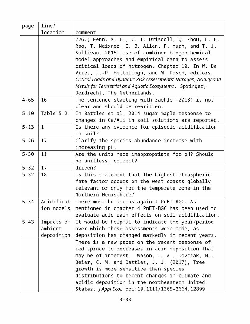
Page 7.18, lines 33-36: The details of this study on the relationship of nitrification to denitrification are simply not important here, and there are dozens of other papers on this topic, if we really want to get into it.

Page 7.18, line 36, through page 7.19, line 23: Here too the report relies heavily on just two studies, and by the same group. There is a much larger and older body of literature here. The present coverage is misleading in that regard.

Page 7.19, lines 28-33: The report needs to specify whether mass unit ratios or molar unit ratios are being used, and someone should go back through the original papers and make sure what is being reported here is accurate in terms of mass or molar, since both are commonly used in the literature.

Page 7.19, lines 31-33: Although I have worked on N vs P limitation of net primary production in aquatic ecosystems for over 35 years, I have no idea what this sentence means…… and I know that at least one of the papers referenced (Schindler 1980) does not support limitation by anything other than P alone. This part of the report needs to be much, much clearer.

Page 7.20, lines 1-2: delete “N/L”

Page 7.20, lines 8-17: Delete this paragraph, which states some highly controversial ideas, and does so with no referencing. I for one do not agree with it as written.

Page 7.20, lines 18-26: Why take a whole paragraph to discuss this one, single paper? I do not see the importance of this study and suggest it be deleted.

Page 7.20, lines 27-37: I like this paragraph, and fully agree with it. However, here still the report is relying on just one paper. This general point of N limitation in oligotrophic settings and P limitation in more productive lakes has been made by others.

Page 7.21, lines 14-28: There is a fundamental confusion here. The Crowley et al. paper dealt with both forests and lakes, and the summary in this report has confused the two: the reported failure of N deposition to drive limitation towards P was for forests, not lakes. The Crowley et al. paper states that lakes were always P limited, regardless of N deposition.

DUE TO TIME CONSTRAINTS, I ONLY QUICKLY SKIMMED PAGES 7.22 TO 7.41.

I was surprised by the large coverage of acid monitoring, relative to very sparse coverage of either nitrogen or eutrophication. Given the national and regional networks for monitoring of surface nutrients and eutrophication, I think is imbalance should be addressed.

Page 7.42, lines 14-28: The Han and Allen (2008) comparison is important, but it is not the only such comparison. The report should, at a minimum, also look at Alexander et al. (2002), Biogeochemistry, 57/58: 295-339.

Page 7.42, lines 24-25: Using a larger data set, Howarth et al. (2012) said 25% is exported.

Page 7.42, lines 29, to page 7.43, line 4: Why pick these particular 3 European studies? On the smaller scale work reported here, there are many, many other recent studies, particularly in Europe. I suggest

B-62

taking a look at the European Nitrogen Assessment as a start, including the chapter by Billen et al. (2011).

Billen, G., M. Silvestre, B. Grizzetti, A. Leip, J. Garnier, M. Voss, R. Howarth, F. Bouraoui, H. Behrendt, A. Lepisto, P. Kortelainen, P. Johnes, C. Curtis, C. Humborg, E. Smedberg, O. Kaste, R. Ganeshram, A. Beusen, and C. Lancelot. 2011. Nitrogen flows from European regional watersheds to coastal marine waters. Pages 271-297 in M.A. Sutton et al. (editors), The European Nitrogen Assessment:  Sources, Effects, and Policy Perspectives. Cambridge University Press.

Page 7.43, lines 5-13: It is fine to use the Haag et al. (2012) study on the Baltic Sea, but please note that was based on earlier work that included watersheds from the U.S. (Howarth et al. 1996, 2006; Boyer et al. 2002), and there are also more recent papers that include the U.S. (Howarth et al. 2012; Hong et al. 2012). All of these papers make the same point, so it is unfortunate to make it seem like only the Swedish study exists.

Page 7.43, lines 17-23: Why focus on this single study as the modeling paper on N cycle within lakes? There must be other examples. I am pretty sure I’ve seen work on how high N loads favor production of volatile organic toxins from cyanobacteria in lakes, for example, which would seem important to mention here.

PAGES 7.44 THROUGH 7.50: Again, time constraints have allowed me to only skim these pages. However, much of the material seems redundant with what I read in chapter 4.

Table 7.6, page 7.52: Only 10 states are listed. Does this mean the other 40 states do not have N criteria for freshwaters? That is simply astounding, if true, and deserves to be highlighted in this report.

Also, as I mentioned above, this report MUST also address N criteria from estuaries and coastal waters.

Pages 7.53 and 7.54: The charts are nice looking, but they come with no real explanation. It is important to explain why the EPA is specifying the regional differences in sensitivity to N that are implied in these charts.

Page 7.55, lines 5-7: I disagree that dissolved oxygen is the widespread indicator of problems with eutrophication in estuaries. Chlorophyll, which can be measured by satellite, is a broader indicator.

Page 7.55, lines 19-21: I find it a little puzzling to give Elser et al. (2007) as the only reference that estuaries tend to be N limited. While I fully agree they tend to be N limited, there are many, many earlier papers that make this case, and I believe more convincingly than Elser et al. (2007). I suggest referencing the NRC 2000 report and Howarth & Marino (2006), as well as Vitousek and Howarth (1991) at the very least for this point.

Howarth, R. W. & R. Marino. 2006. Nitrogen as the limiting nutrient for eutrophication in coastal marine ecosystems: Evolving views over 3 decades. Limnol. Oceanogr. 51: 364-376.

Page 7.55, line 30, to Page 7.56, line 5: The story of acidification is a little more complicated than stated here, not just algae dying and decomposing: production of carbon by seagrasses is also important, and respiration by living algae and seagrasses during the night can also contribute to acidification. Note

B-63

that in a eutrophic seagrass bed we studied in Massachusetts, there was a very pronounced diel pattern in pH, with moderate pHs during the day, but by dawn, very acidic waters driven by this respiration by living algae and seagrasses overnight. See the following paper: Howarth, R.W., M. Hayn, R.M. Marino, N. Ganju, K. Foreman, K. McGlathery, A.E. Giblin, P. Berg, and D. Walker. 2014. Metabolism of a nitrogen-enriched coastal marine lagoon during the summertime. Biogeochemistry 118: 1-20.

Page 7.56, lines 8-10: I disagree that deposition is typically less than half the N inputs to estuaries. As I discussed in Howarth (2008a, 2008b), I think the evidence points to N deposition being perhaps half of the total N load to Chesapeake Bay and Barnegat Bay, and quite likely more than that in New England estuaries such as Casco Bay and Great Bay. Also, keep your Tampa Bay example in mind….

Page 7.56, lines 28-31: The Howarth et al. (2002) reference is fine, but I suggest also adding in Howarth (2008a) and (2008b). And as I stated just above, I disagree with characterizing the atmospheric input to estuaries as generally less than half.

Pages 7.57, 3-15: As with earlier in the Chapter, keep the regional differences in mind: yes, NOy deposition is going down across the U.S., and NHy deposition up. But that means lower deposition overall throughout most of the East coast. Also, this section seems very dated, with the most recent references from 2008. Surely, there has been new work on the change in deposition since then? For instance, hasn’t the Chesapeake Bay Program reported decreased N loads from the Susquehanna River over the past decade, due to lower atmospheric deposition?

Table 7.8, starting on page 7.59: As per my 2008 critique, I believe the SPARROW model underestimates the importance of atmospheric deposition, since it relies on wet deposition as the surrogate for total deposition; the relative importance of dry gaseous N deposition in urban and suburban areas (near NOx emission sources) is far higher than in rural areas, introducing a major bias to the SPARROW results.

Also, note that while Boyer et al. (2002) do indeed give an average relative importance of atmospheric deposition of 31%, the values for watersheds in northern New England were substantially higher; there, atmospheric deposition dominated. This is important to point out in the table and Boyer et al. (2002) are probably underestimating N deposition in urban and suburban areas.

Page 7.60, line 13, through page 7.61, line 2: Again, I believe many of these underestimate the importance of atmospheric deposition. Note in particular that I am quoted as saying the importance is 25% in Howarth (2007); that paper was actually published in 2008 (it is 2008b above), and I said up to 50%.

Pages 7.61 through 7.62: I have again skimmed this work; a lot of studies are included, but the selection of papers seems random and not comprehensive, and the section is written in a non-synthetic way. Are all of these studies of equal value and validity? I do not think so, and yet that is the impression one gets.

Page 7.62, lines 24-27: The statement on the importance of lightning as an N source just before landfall by a hurricane needs to be qualified, or deleted. Otherwise, the reader may come away with the thought

B-64

that lightning rather than human activities is a general problem, which is simply not the case. Lightning dominated for a very, very brief time. This is interesting, but not important.

Page 7.62, line 31, to page 7.63, line 4: This paragraph on the influence of climate change is very brief, and very light on referencing. In Howarth et al. (2012), we demonstrated larger N fluxes (larger percent delivery of human N inputs) in wetter climates with more discharge, across 150 different watersheds. And in Howarth et al. (2011), we review several mechanisms whereby the climate change that has already occurred over the past decade or so has made estuaries and coastal marine ecosystems more sensitive to the adverse effects of N pollution. See also Naijar et al. (2010) for a review of possible climate change impacts on Chesapeake Bay, including how these interact with N pollution, and Howarth et al. (2000) for a study on the Hudson River estuary in NYC harbor.

Howarth, R. W., G. Billen, F. Chan, D. Conley, S. C. Doney, J. Garnier, and R. Marino. 2011. Coupled biogeochemical cycles: Eutrophication and hypoxia in coastal marine ecosystems. Frontiers in Ecology & Environment 9: 18-26.

Howarth, R. W., D. Swaney, G. Billen, J. Garnier, B. Hong, C. Humborg, P. Johnes, C. Morth, and R. Marino. 2012. Nitrogen fluxes from large watershed to coastal ecosystems controlled by net anthropogenic nitrogen inputs and climate. Frontiers in Ecology & Environment 10: 37-43.

Howarth, R.W., D. Swaney, T. J. Butler, and R. Marino. 2000. Climatic control on eutrophication of the Hudson River estuary. Ecosystems 3: 210-215.

Naijar, R., C. R. Pyke, M.B. Adams, D. Breitburg, C. Hershner, M. Kemp, R. Howarth, M. R. Mulholand, M. Paolisso, D. Secor, K. Sellner, D. Wardrop and R. Wood. 2010. Potential climate-change impacts on the Chesapeake Bay. Estuarine and Coastal Shelf Science 86: 1-20.

Page 7.63, lines 5-10: As I wrote above, I find it a little puzzling to give Elser et al. (2007) as the only reference that estuaries tend to be N limited. Here, I suggest deleting Elser et al. (2007), and instead simply use NRC 2000, or perhaps that plus Howarth and Marino 2006.

Page 7.63, lines 11-26: This is a long, qualitative discussion (particularly when it comes to atmospheric deposition of N), and based heavily on a 2002 reference. I suggest using more recent material, and making this more quantitative, or deleting.

Page 7.65, lines 1-15: Here, we are returning to the style earlier in the Chapter of having large paragraphs devoted to describing one or two studies, often site-specific as in this case. There is a very much larger body of literature out there, making the choice of these particular studies very puzzling. The studies are not unique…. What is the point that EPA is trying to develop here?

Page 7.65, lines 16-22: There is a large body of literature on the importance of denitrification, and the two studies cited here fail to do that justice. In fact, the study cited that claims denitrification is not important is very much an outlier: denitrification is a very important sink for N in most estuaries. See the 1996 review by Nixon et al. (Biogeochemistry, 35: 141-179). For an example of its importance in a recent study, see Hayn et al. (2013).

B-65

Hayn M., R.W. Howarth, R. Marino, N. Ganju, P. Berg, K. Foreman, A.E. Giblin, and K. McGlathery. 2013. Exchange of nitrogen and phosphorus between a shallow lagoon and coastal waters. Estuaries & Coasts doi10.1007/s12237-013-9699-8

Page 7.65, lines 23-27: This brief paragraph focuses equally on denitrification and ANAMOX, but ignores the dissimilatory reduction of nitrate to ammonium (DNRA), a process that was little understood in estuaries as of 2008. The paragraph needs to be expanded to include this, and to better discuss denitrification and its controls; I would not expand on ANAMOX, as this is generally not an important process in most estuaries. And this should definitely include the Nixon et al. (1996), Biogeochemistry 35:141-179, review which is a critical part of our understanding (for the time before DNRA was fully appreciated).

Page 7.65, lines 28 through line 2 on page 7.57: Delete this paragraph, as it contributes little or nothing towards understanding the larger issues upon which this report should be focused. It is very detailed microbiology, taken out of the context of why this might matter in terms of N deposition and estuaries.

Page 7.66, lines 3-11: Since the section title says “sediment processes and DO,” I suggest qualifying in the first sentence that you are talking about DO in the water column (since estuarine sediments are almost always largely devoid of oxygen below 1 mm or so). Also, most of this section is actually on water-column hypoxia, and not sediment processes at all; so I suggest changing the title to “DO and hyopoxia.”

Also, the causes of low DO need to be broadened: it is not simply about the decomposition of dead organic matter. The respiration of living algae and seagrasses can also lower DO to very low levels, as seen in the deeper portions of the Hudson River estuary where phytoplankton are mixed into the dark for long periods of time (Howarth et al. 1996), and as seen every night in a eutrophic seagrass-dominated system on Cape Cod (Howarth et al. 2014).

Howarth, R.W., R. Schneider & D. Swaney. 1996. Metabolism and organic carbon fluxes in the tidal, freshwater Hudson River. Estuaries 19: 848-865.

Howarth, R.W., M. Hayn, R.M. Marino, N. Ganju, K. Foreman, K. McGlathery, A.E. Giblin, P. Berg, and D. Walker. 2014. Metabolism of a nitrogen-enriched coastal marine lagoon during the summertime. Biogeochemistry 118: 1-20.

Page 7.68, lines 11-23: acidification is driven not simply by decomposition of dead material, but can also be the result of CO2 produced by respiration of algae and seagrasses. Howarth et al. (2014) demonstrated high acidity (low pH) every night in a eutrophic seagrass system. This was driven by respiration of the living plants and algae; during the day, as CO2 was drawn down through primary production, the pH steadily climbed and was no longer as acidic, although the net effect was to drive acidification, due to slow exchange of CO2 with the atmosphere.

Howarth, R.W., M. Hayn, R.M. Marino, N. Ganju, K. Foreman, K. McGlathery, A.E. Giblin, P. Berg, and D. Walker. 2014. Metabolism of a nitrogen-enriched coastal marine lagoon during the summertime. Biogeochemistry 118: 1-20.

Section 7.3.3.1, pages 7.68 to 7.70: this section on modeling is strong, a welcome reprieve after reading the earlier material in this chapter.

B-66

Section 7.3.3.2: This section too is well done.

Section 7.4.2, pages 7.77 to 7.78: This summary on the N biogeochemistry in estuaries is very short, certainly in comparison to the summary on freshwaters that precedes it. Given that N pollution is the major cause of harm to the majority of the estuaries in the U.S. (NRC 2000; Bricker et al. 2007), this section really needs to be strengthened and expanded.

Chapter 10:

Page 10.2, lines 2-6: The CO2 that drives acidification is not just from decomposition of dead material; during the night, respiration of living algae and seagrasses can also drive substantial acidification. See Howarth et al. (2014).

Howarth, R.W., M. Hayn, R.M. Marino, N. Ganju, K. Foreman, K. McGlathery, A.E. Giblin, P. Berg, and D. Walker. 2014. Metabolism of a nitrogen-enriched coastal marine lagoon during the summertime. Biogeochemistry 118: 1-20.

Page 10.2, lines 27-30: I agree with this statement that estuaries tend to be N limited, but I would not use Elser et al. (2007) as the sole reference: that was largely a meta-analysis of short-term bioassays, and the bioassay approach has been heavily criticized by many. I suggest adding two references that address this concern, and yet still conclude that estuaries are largely N limited: our NRC (2000) report, and Howarth & Marino (2006). Further, note that both NRC (2000) and Howarth & Marino (2006) stated that some estuaries are P limited, or colimited by N & P, or switch seasonally between N and P, although N limitation alone dominates.

Howarth, R. W. and R. Marino. 2006. Nitrogen as the limiting nutrient for eutrophication in coastal marine ecosystems: Evolving views over 3 decades. Limnol. Oceanogr. 51: 364-376.

Also, in this regard, David Schindler and others have argued that only a whole-ecosystem experiment can demonstrate N limitation, and he further stated there have been no such experiments in estuaries. We address this concern in Howarth et al. (2011) and in the Howarth et al. (2014) study (see above), we present data from an inadvertent whole-ecosystem N addition that clearly shows the estuary to be N limited.

Howarth, R. W., G. Billen, F. Chan, D. Conley, S. C. Doney, J. Garnier, and R. Marino. 2011. Coupled biogeochemical cycles: Eutrophication and hypoxia in coastal marine ecosystems. Frontiers in Ecology & Environment 9: 18-26.

Page 10.4, lines 1-12: I read this after writing the comments immediately above; these lines are well done, but I still suggest integrating in some of my thoughts from just above.

Page 10.4, lines 22-28: This section on the importance of atmospheric deposition relies on Chapter 7, where I have argued major revisions are needed. So this summary should also be updated and the use of only references from 2008 for the shift in rates of deposition is problematic; there is a much larger, more recent literature out there on decreased NOy deposition and increased NHy deposition.

B-67

Section 10.1.2, beginning on page 10.5: this short, qualitative summary is completely redundant with Chapter 7. I suggest deleting it, or updating it after Chapter 7 is revised.

Page 10.8, lines 5-10: It is worth noting that the most heavily N-loaded estuary in North America (the lower Hudson, NYC harbor estuary) has few if any negative consequences, due to the very rapid flushing of this ecosystem: phytoplankton are flushed away as fast as they can grow.

Howarth, R., D. Swaney, T. J. Butler, and R. Marino. 2000. Climatic control on eutrophication of the Hudson River estuary. Ecosystems 3: 210-215.

Howarth, R. W., R. Marino, D. P. Swaney, and E. W. Boyer. 2006. Wastewater and watershed influences on primary productivity and oxygen dynamics in the lower Hudson River estuary. Pages 121-139 in J. S. Levinton & J. R. Waldman (eds.), The Hudson River Estuary, Cambridge Univ. Press.

Page 10.9, lines 9-10: I disagree with the suggestion that DIN is a reliable indicator of N inputs or eutrophication. In the highly eutrophic seagrass system we have studied on Cape Cod, DIN levels are always very low (< 1 uM) despite the very high N load; the DIN is simply taken up too rapidly by the primary producers. See Howarth et al. (2014), referenced above.

Page 10.22, lines 18-20: low dissolved oxygen results not just from decomposition of dead organic matter: the respiration of living algae and seagrasses can also lower DO to very low levels, as seen in the deeper portions of the Hudson River estuary where phytoplankton are mixed into the dark for long periods of time (Howarth et al. 1996), and as seen every night in a eutrophic seagrass-dominated system on Cape Cod (Howarth et al. 2014). In this seagrass system, hypoxia is common at dawn after hours of darkness, while oxygen levels are supersaturated at the end of the daylight period.

Howarth, R.W., R. Schneider & D. Swaney. 1996. Metabolism and organic carbon fluxes in the tidal, freshwater Hudson River. Estuaries 19: 848-865.

Howarth, R.W., M. Hayn, R.M. Marino, N. Ganju, K. Foreman, K. McGlathery, A.E. Giblin, P. Berg, and D. Walker. 2014. Metabolism of a nitrogen-enriched coastal marine lagoon during the summertime. Biogeochemistry 118: 1-20.

Page 10.26, lines 23, through page 10.27, line 18 (and Table 10.4): In the Howarth et al. (2014) study referenced above, we observed a significant dieback of seagrasses in a eutrophic harbor in 2010, and clearly tied it to the elevated nitrogen load.

Page 10.44, lines 11-20: Add reference to Howarth et al. (2014), referenced above, where we showed a very pronounced diel pattern in pH in an N-enriched seagrass ecosystem: pHs were very acidic every dawn at the end of the dark period.

B-68

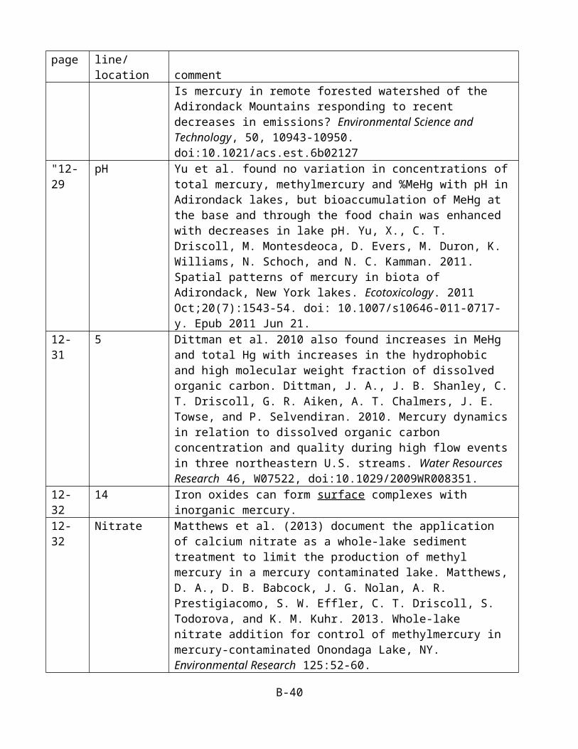
Dr. Donna Kenski

My comments are limited to Charge Questions 1, 2, and 15, reviewing the Executive Summary, Chapters 1 and 2, and Appendix C. PrefaceThis section is mostly fine as it is strictly historical, but it gives short shrift to the reasons behind the failure to set a new secondary standard after the last review. A more expansive explanation of the metric that was developed and why it was found inadequate would be useful background for this new review cycle. In particular, because the primary issue with the proposed indicator in the last review was uncertainty, it helps to set the stage for this review and highlights the need to clarify and quantify uncertainties wherever possible. The Integrated Review Plan contained such a summary in its section 4.1.1.7 that could form the basis of such a discussion. This Preface, or subsequent sections, should also address the problem of controlling deposition effects with a concentration-based standard. By clearly laying out this fundamental problem early in the process, EPA will help all concerned to be mindful of the structure in which a potential standard must be developed.Minor comments:p. xlv: SRP is defined in the glossary as soluble reactive phosphorus but actually used in the text for sulfate-reducing prokaryotes

Executive Summary Great job summarizing a huge amount of information. I appreciate the clear distinction between new data and findings and old data and findings that were covered in the previous ISA. The use of hyperlinks to jump to relevant sections of the document and references is a great help. p. lxii, line 19: More current SO2 emissions data is available and is given later in the report; please update these values to reflect the most recent data.p. lxvi, first table entry, lateration -> alterationp. lxvii, line 21, statement is misspelled

line 23, remove extra periodp. lxxii, line lxxii: existing is misspelled

Chapter 1This more expansive summary of the document is also well done and generally has an appropriate level of detail. As in the Executive Summary, the use of hyperlinks is very helpful, although they are not always consistently applied. More frequent use of links to the summarized sections would be helpful. Also, the use of boldface type for emphasis when confirming one of the causal determinations is a nice touch. In direct answer to the charge question, the causal framework has been appropriately applied and the causal determinations have been adequately documented. Section 1.2.2, Measurement and Modeling Techniques, refers to deposition rates that are ‘highly uncertain.’ Every effort should be made to give quantitative uncertainties wherever possible. Similarly, Section 1.2.3, Spatial and Temporal Variability in Deposition, summarizes the TDEP estimation of annual dry and wet deposition of S and N, but characterizes fluxes as subject to ‘sizable uncertainty’. This summary chapter should have a more quantitative discussion of the uncertainties that are inherent in the estimation of deposition and deposition flux. These uncertainties are discussed at some length at various places in Chapter 2, with an important figure 2-33 that shows both N and S fluxes and

B-69

uncertainties; either address the uncertainties individually in the section summaries or add a section just for uncertainty sources and magnitudes. p. 1-12, lines 7, 12, and 13: “or NH3” should be “and NH3”

line 31: remove comma after NOxp. 1-19, line 12: thesame -> the samep. 1-21, line 5: “is it” -> it isp. 1-56, line 24: where -> werep. 1-63, line 8: should be “…watersheds, estimates of…”

line 9: ANC -> ANCsp. 1-78, lines 18-21: Should this causal statement be bold?p. 1-81, line 3: SRP hasn’t been previously defined, should be sulfate-reducing prokaryotesp. 1-81, line 4: Should this be Section 12.2.5?p. 1-85, Section 1.12: this section just ends abruptly without a real summary or conclusion.

Chapter 2, Source to DepositionChapter 2 is generally well written and thorough, but perhaps could benefit by being shortened and summarized. The sheer volume of information is overwhelming. There’s a lot of detailed chemistry of the various nitrate and sulfate species, but it’s difficult to assess the relative importance of the various species and their reaction pathways. Of course it will vary by geography and weather and a host of other factors, but some attempt to summarize is warranted. Section 2.4, Atmospheric Transport, seemed out of place. Perhaps it would be better as part of a discussion of chemical transport models. Comparisons of various models are sprinkled throughout the document, but there isn’t any comprehensive discussion of model performance for concentration or deposition for the major contenders: CAMx, CMAQ, GEOS-CHEM, hybrid satellite/CTMs. Because modeling is so integral to the estimation of N&S deposition, it needs a thorough review in the ISA.

Section 2.5 is not very straightforward in its discussion of the various monitoring networks. I was taken aback at the realization that the FRM NO2 network is not considered relevant for deposition. This section never clearly states why, although the reasoning is given succinctly in the Chapter 2 summary on p. 2-88. This helpful discussion from the summary, Section 2.11, should first appear in Section 2.5.1. A general review of the adequacy of the monitoring data to support deposition estimates and modeling should be included in the ISA. The majority of the science reviewed here depends directly on the data from CASTNET, NADP, and IMPROVE, yet the existence of these networks has become increasingly tenuous. The ISA should document the quality and adequacy (spatial and temporal coverage) of the monitoring networks that provide the basis for the much of the deposition science contained in this review.

Section 2.7.2 seemed excessively detailed and could be shortened if flux measurements were described conceptually without the math. Section 2.8.4 presents important data on hybrid satellite/model estimates of deposition flux and uncertainty, but the accompanying Fig. 2-33 is barely legible. Higher resolution images of this data should be obtained if possible. Also, the uncertainties are given in mass units and the text summarizes uncertainty over the entire study area as 30%; more information on the spatial distribution of uncertainties is desirable. One question I still have, which I hoped the ISA would answer, is whether the hybrid satellite/CTM models are demonstrably better than CTMs alone in estimating deposition of the relevant species. As noted above, a comprehensive comparison of model performance is needed.

B-70

Section 2.9 on transference ratios is interesting and new since the last review. Is this mechanism for linking ambient concentrations to deposition a potential basis for a secondary standard? If so, more updated information will need to be provided. As the text notes, older versions of models were used and some errors in inputs were identified. The data presented don’t provide a high degree of confidence, but the method seems promising. More details, please!

Oddly, the summary section again brings up data that was not earlier discussed in the Chapter (unless I missed it, always a possibility…). On p. 2-89, the middle paragraph compares, in very general terms, two micrometeorological models (MLM and BLM) but this comparison and the BLM were not mentioned previously. p. 2-6, line 23: not clear. NH3 is not an example of a fugitive source.Line 28: oxidized is misspelled.Line 31: entries is an odd word; estimates or data would be a better choice.Line 35: chemical transport model, not chemistry transport model or chemistry-transport model. This error occurs multiple times throughout the chapter. p. 2-23, line 21: delete ‘for’; should be Community Multiscale Air Quality (CMAQ) modeling system. This error also occurs in several places.p. 2-27, line 8: capitalize ‘the’.Line 28: Bonville -> Bondvillep. 2-32, Fig. 2-8: Add units to these plots (ppbv)p. 2-38, Fig. 2-10: These plots aren’t legiblepp. 2-39, 2-40, 2-45, 2-67, 2-68: The color scales for these plots lose too much detail; they should be redrawn to show more variation at low concentrations. Also, the captions incorrectly define CASTNET as Clear Air Status and Trends, rather than Clean Air Status and Trends. This is another error that occurs multiple times in figures and text. Please search and replace.p. 2-44, Fig. 2-15: CASTNET and CMAQ definitions are both wrong. Last sentence of caption has repeated phrase ‘can be’. Delete close paren after billionp. 2-48, line 27: delete ‘to’. Also, rho in Equation 2-12 is not defined. Should be density of air, same as Equation 2-13p.2-49, line 26: should be hyphens or dashes between NH3-HNO3-NH4NO3.p. 2-64: Figs 2-22a and b are exact inverses of each other so only 1 is really necessary.p. 2-87, line 2: need a comma after CONUS.Line 16: pulse -> pulsedLine 36: delete ‘could’, add comma after sources. Appendix C:The case studies in Appendix C covered a representative selection of areas with significant impacts from N&S deposition, although I concur with other committee members request to include a case study on the Adirondacks as well. The material presented was adequately detailed although it was not always consistent in presentation. Each of the case studies should have a summary either at the end or beginning; currently only the Southern CA case study does.

B-71

Dr. William McDowell

Chapter 7

7-4 line 9: Flat Head Lake, MT = Flathead7-26 line 23: “As a result of this widely observed pattern, surface water DOC concentration has become a more important indicator of acidification and chemical recovery since the 2008 ISA” This is true, to the extent that surface water recovery from acidification has been associated with increases in DOC at many sites. It is not strictly true that DOC concentration is an indicator of recovery, however. Recovery has been documented to occur in many sites without a change in DOC. This is a data and understanding gap – why are some sites showing increase in DOC with decreased acid deposition, and others show no change in DOC? At present there is no widely accepted mechanism to explain these observations, and few studies that assess the extent to which a regionally representative sample of lakes has increased in DOC concentration. 7-26 line 11: “The 2008 ISA reported widely observed increased concentrations of DOC in surface waters across North America and Europe and that these increases in DOC were at least partly related to changes in atmospheric deposition of S and N. Thus, it has been recognized for several decades that surface water DOC concentrations have decreased to some extent with water acidification and, therefore, would likely increase with recovery.” The last sentence is incorrect. These increases and implications for recovery have been recognized for about a decade, not decades. The same text repeated in the Summary, and is incorrect there, as well. 7-27 line 2: “changes in DOC concentration {increases} might reduce the ability of inland waterways to remove reactive N from the aquatic ecosystem.” This is not entirely correct. Other studies specifically address DOC and NO3 removal, and report an opposite conclusion: they show that NO3 removal is greater in systems with higher DOC concentrations and higher ratios of DOC:NO3 (Rodriguez-Cardona et al. 2016; Wymore et al. 2017), suggesting that complex interactions exist between DOC and N cycling.

Rodríguez-Cardona, B., A.S. Wymore, and W.H. McDowell. 2016. DOC:NO3- ratios and NO3

- uptake in forested headwater streams. Journal of Geophysical Research Biogeosciences 121:205-217. doi:10.1002/2015JG003146

Wymore, A.S., A. Coble, B. Rodriguez-Cardona, and W.H. McDowell. 2016. Nitrate uptake across biomes and the influence of elemental stoichiometry: A new look at LINX II. Global Biogeochemical Cycles 30:1183-1191.

7-34 line 26: “The relationship between ultraviolet (UV) absorbance and DOC concentration has been shown to reflect changes in the proportion of DOC that is hydrophobic (aromatic, recalcitrant) and thus resistant to biodegradation.” While these relationships can hold true for some sites and circumstances, it is really only appropriate to say that UV absorbance reflects the aromaticity of the DOC components. Inferring other general attributes like biodegradability is not supported by the literature. 7-40 line 22: “Relatively modest increases over time in pH and ANC were commonly observed {in Europe} in response to decreased levels of acidic deposition.” In the Czech Republic (Oulehle et al. 2008, Oulehle et al. 2016) responses have been quite large, so this broad generalization seems to be poorly supported. They also show unexpected interactions between N and P may also be affecting the trajectory of recovery (Oulehle et al. 2017).

B-72

Oulehle, F., W.H. McDowell, J.A. Aitkenhead-Peterson, P. Krám, J. Hruška, T. Navrátil, F. Buzek, and D. Fottová. 2008. Long-term trends in stream nitrate concentrations and losses across watersheds undergoing recovery from acidification in the Czech Republic. Ecosystems 11:410-425.

Oulehle, F., T. Chuman, J. Hruška, P. Krám, W.H. McDowell, O. Myška, T. Navrátil, and M. Tesař. 2017. Recovery from acidification alters concentrations and fluxes of solutes from Czech catchments. Biogeochemistry 132:251-272. DOI 10.1007/s10533-017-0298-9

Table 7.6: California NO3-N criteria of 45 mg/L seem suspect, as it is well above the WHO drinking water standard. Check units.

Chapter 8

Overall, Chapter 8 is well written and thorough. I have no line-specific edits, but instead offer the following observations:

It is apparent when comparing the biotic response to acidification in terrestrial and aquatic systems that there is a relative lack of information on aquatic biological response (beyond eutrophication). This should be noted, as it suggests that there is greater uncertainty in quantifying the magnitude of the biotic response in aquatic vs terrestrial systems.

For aquatic biota, biotic interactions are often important in driving community structure, and they can obscure or magnify the impacts of atmospheric deposition. For amphibians, the big issue globally for the last decade has been chytrid fungi. They should at least be mentioned, though it is possible that their prevalence or impacts in temperate, acid-sensitive surface waters are unknown. For fish in acid-sensitive surface waters, species introductions by anglers or state agencies can have large impacts on community structure. These issues should be acknowledged.

Chapter 12

This chapter presents a detailed overview of the effects of sulfur enrichment. The accuracy, level of detail, and relevance of information presented on the biological effects of sulfide phytotoxicity and the mechanisms linking sulfur and mercury methylation are adequate. What is lacking, however, is an overview that links the cause-effect chains that are embedded in the detailed analysis.

There is some redundancy in the sections, and the topics addressed therein. I suggest the following reorganization:12.1 Introduction and causal statements12.2 Effects of sulfur deposition on the sulfur cycle as written12.3 Interactions between S deposition and Hg12.3.1 Hg cycle and the importance of methylation12.3.2 Sulfate-reducing prokaryote biology and genetics12.3.3 Drivers of Hg methylation potential: physiological response of SRPs and rates of methylation to various drivers such as DOC, pH, etc.12.3.4 Deducing the strength of drivers under field conditions from whole-system field experiments12.3.5 Inferring the strength of drivers from assessment of patterns in drivers and MeHg under ambient conditions.

B-73

Dr. Erik Nelson

Comments on Chapter 13

1. Broad Concepts and Issues :

Should this be a stand-alone chapter or should each previous chapter discuss the potential impacts on N and S deposition and cycling in the relevant ecosystem type due to climate change?

When reading and commenting on the ISA, including chapter 13, we need to constantly ask ourselves how the final ISA will best be able to assist the writers of the eventual REA and policy assessment (PA). How can the ISA summarize the peer-reviewed literature in a way that will allow REA and PA authors to create a high quality document? 

2. Key Issues for Charge Question 13:

I think it is important to reiterate to the reader that climate change will modify the processes already discussed in the ISA. And that because climate change is so uncertain the reader needs to understand that the ISA tends to use generalizations when discussing potential modification and avoids specific predictions of impacts. However, to the extent that the ISA can identify what modifications are the most important or will modify the already identified processes the most, the better. By doing so, the ISA authors will help the PA authors immensely. Further, to the extent that ISA authors can present ranges in expected modifications die to climate change, no matter how broad the range, the better.

Throughout Chapter 13 we see the statement: “Potential future changes in the quantity and temporal distribution of precipitation and temperature (and their interactions) is expected to alter the wet-dry cycles that govern [some dynamic].” Therefore, can the ISA authors include a summary of expected changes across the US in the quantity and temporal distribution of precipitation and temperature?

Won’t climate change affect the dynamic and rate of acidification due to sulfur deposition? If so there needs to be some mention of this potential in this chapter.

There is no discussion on the transport and transformation of nitrogen in ecosystems dominated by monoculture agriculture. For example, how will additional N and S deposition due to climate change affect crop growth and the non-point water pollution issues that are bedeviling the Midwest? Ultimately, these effects need to be assessed if we are to get a fuller picture of the welfare impacts of additional N and S deposition on the US landscape and how climate change may modify these welfare impacts.

Further, as noted in the ISA, the rate and impact of N transport and transformation will be affected by climate change. Changes in temperature and precipitation patterns are and will continue to very across the country. Therefore, can the ISA authors find a way to assess and summarize the expected changes in rate and impact of N transport and transformation due to climate change by region? For example, how will expected climate change affect rate and impact of N transport and transformation differently in the in the Pacific Northwest than it will in the Midwest?

A regional analysis would also be helpful for Section 13.1.2.2. In this section the authors note that variation of acidification events across the U.S. may be exacerbated due to climate change. Can the

B-74

authors indicate how climate change may affect future acidification events and their variability across the various regions of the U.S.? In Section 13.1.2.1 it is noted that changes in N transport and transformation due to climate change will affect the rate of C sequestration in soil and biomass. For example, as the ISA says on page 13-6, “[o]ur synthesis of existing meta-analyses indicates that aboveground NPP is highly responsive to N addition and enhanced precipitation, while temperature rise does not increase aboveground NPP.” And on page 13-8, “[a] meta-analysis of N addition studies indicates that adding N to grasslands had no effect on NEE, but that N addition increased forests EC (Liu and Greaver, 2009).” How in accurate will models of C sequestration be if they fail to incorporate this climate change-induced dynamic? C sequestration models are used more and more to determine climate change policy. Therefore, they need to be as accurate as possible. It appears some researchers have incorporated climate change-induced changes in the N cycle into C sequestration models. For example, see Hartman, M. D., Baron, J. S., Ewing, H. A., & Weathers, K. C. (2014). Combined global change effects on ecosystem processes in nine US topographically complex areas. Biogeochemistry, 119(1-3), 85-108.

3. Secondary Issues for Charge Question 13:

It would be great if the authors of the ISA could put the expected changes in rate and impact of N transport and transformation into some sort of context. Such an analysis would greatly help the writers of the REA and PA. For example, is there any literature that suggests how much more N will be available for animal and plant use given climate change versus a climate change-free counterfactual?

I am not sure what to make of Section 13.1.2.3. It is a grab bag of ways that additional N and N-based acidification, and the way that these dynamics may be affected by climate change, may affect biodiversity. I suspect that this section is too vague to help writers of the PA.

Comments on Chapter 14

This is the first chapter to explicitly discuss the links between the biophysical dynamics discussed in this ISA and human welfare. There should be a paragraph or two that explains why this chapter is in the ISA. In some respects, this is the chapter that links the ISA to REA and PA. Remember it is the human impacts of the biophysical dynamics discussed in this ISA that will be used to ultimately decide the NAAQS standard.

First, the cataloging of the various ecosystem service frameworks is unnecessary (pages 14-1 – 14-2). Instead state what an ecosystem service is and summarize in a table all the ecosystem services in the U.S. that are affected by Oxides of Nitrogen, Oxides of Sulfur, and Particulate Matter. Further, this table should also indicate the services that are particularly sensitive to N and S deposition.

In Section 14.1.1 a table that summarizes the ecosystem service damage estimates from additional N would be more helpful then the two figures. This table could break down damage estimates by region and service.

Further, it is not clear to me which studies separately quantify ecosystem service damages from the atmospheric portion of additional N loading. Therefore, the proposed summary table could also separate ecosystem service damages due to the atmospheric portion of additional N loading from the damages due to the terrestrial portion of N loading.

B-75

There are a slew of papers on the projected impact of ocean acidification on fisheries. A Google Scholar search on “the economic impact of ocean acidification U.S.” will turn them up. A table that summarizes these estimates for U.S. fisheries would be great. (Examples: Mabardy, Rebecca A., et al. "Perception and response of the U.S. West Coast shellfish industry to ocean acidification: the voice of the canaries in the coal mine." Journal of Shellfish Research 34.2 (2015): 565-572.

Overall this chapter needs to do a better job of delineating estimated ecosystem service damages due to additional atmospheric N versus estimated ecosystem service damages due to additional terrestrial N. It aloes has to do a better job of displaying the range in damage estimated from additional N.

Comments on appendices

1. Can the authors add a “Lessons Learned” section? In this section the authors would summarize the similarities and differences across case studies, common ecological impacts from N and S deposition, identify what polices or approaches have been effective at reducing N and S deposition, identify what polices or approaches have been effective at helping ecological systems adapt to higher levels of pollution, and a summary of human welfare impacts across the regions due to higher levels of N and S-based pollution.

2. Could the authors project what will happen in the case study areas under current NAAQS standards? For example, the authors could extrapolate the curves in Figures C-5, C-9, C-10, C-15, C-25, and C-37 and then compare these trends against critical loads and current NAAQS standards. I think such an analysis would be helpful for all, especially as we move forward and make a judgment on whether a stricter standard is needed.

B-76

Dr. Hans Paerl

Chapter 7

Fig. 7.1 on P. 588: There's no mention of denitrification in this figure, even though it depicts the N cycle.

P. 595, lines 10-12, add reference to support statement: Paerl, H. W., J.T. Scott, M.J. McCarthy, S.E. Newell, W.S. Gardner, K.E. Havens, D.K. Hoffman, S.W. Wilhelm and W.A. Wurtsbaugh. 2016. It takes two to tango: When and where dual nutrient (N & P) reductions are needed to protect lakes and downstream ecosystems. Environmental Science & Technology 50: 10805−10813.

Chapter 9

P. 733, lines 24-26, it is stated: “N limitation appears to be increasingly common in freshwater systems, probably because their nutrient dynamics are being altered significantly by growing agricultural and urban P inputs.” Please add the following recent reference:Paerl, H. W., J.T. Scott, M.J. McCarthy, S.E. Newell, W.S. Gardner, K.E. Havens, D.K. Hoffman, S.W. Wilhelm, and W.A. Wurtsbaugh. 2016. It takes two to tango: When and where dual nutrient (N & P) reductions are needed to protect lakes and downstream ecosystems. Environmental Science & Technology 50: 10805−10813.

P. 734, Figure 9.2: Denitrification is missing in this figure of the N cycle.

P. 735, lines 7-9: It is stated that “In highly productive freshwaters, nutrient enrichment from N deposition usually does not stimulate primary productivity or community change because P is more commonly the limiting nutrient.” This is not necessarily true. N limitation tends to be more prevalent in highly eutrophic lakes:See Elser 2007 (cited in the report).Also: Paerl, H. W., J.T. Scott, M.J. McCarthy, S.E. Newell, W.S. Gardner, K.E. Havens, D.K. Hoffman, S.W. Wilhelm, and W.A. Wurtsbaugh. 2016. It takes two to tango: When and where dual nutrient (N & P) reductions are needed to protect lakes and downstream ecosystems. Environmental Science & Technology 50: 10805−10813.

P. 735, lines 28-29: Add: Paerl, H. W., J.T. Scott, M.J. McCarthy, S.E. Newell, W.S. Gardner, K.E. Havens, D.K. Hoffman, S.W. Wilhelm, and W.A. Wurtsbaugh. 2016. It takes two to tango: When and where dual nutrient (N & P) reductions are needed to protect lakes and downstream ecosystems. Environmental Science & Technology 50: 10805−10813.

P. 738, lines 10-14: It is stated that “This pattern of increasing P limitation with increasing N deposition in the Adirondack sub-region was also evident in foliar N:P ratio from seven tree species examined in the same study. Tree and lake data did not support a transition from N toward P limitation for the entire five-state region, but that shift was supported for the Adirondack sub-region.” We need to be careful here. Inferring nutrient limitation from N:P ratios can be tricky, especially if one or both nutrients are saturating.

This comment also applies to lines 19-21.

B-77

Chapter 10

P. 776, lines 3-6: It is stated that, “Increased production of CO2 from degradation of organic matter associated with eutrophication along with atmospheric anthropogenic CO2 inputs can result in formation of carbonic acid and make the ocean water more acidic.” This is still quite speculative, especially the degradation of organic matter part. Eutrophication will also lead to enhanced uptake of CO2 due to higher rates of primary production. How can you have more CO2 released by mineralization than is produced by what is fixed due to eutrophication?

P. 777, Figure 10-1: Delete "concentration of available nutrients" and substitute "availability of nutrients".

P. 778, line 4: Insert “excessive” before “N”.

P. 778, lines 26-28: It is stated that “atmospheric deposition of reduced N has increased relative to oxidized N and this trend is expected to continue in the future under existing emission controls (Pinder et al., 2008; U.S. EPA, 2008a).” The increase in atmospheric reduced N is a troubling trend, as this form of N is highly bioreactive and often a preferred source of N for phytoplankton, including harmful species (Glibert et al., 2016).

Glibert, P., F. Wilkerson, R. Dugdale, J. Raven, C. Dupont, P. Leavitt, A. Parker, J. Burkholder and T. Kana. 2016. Pluses and minuses of ammonium and nitrate uptake and assimilation by phytoplankton and implications for productivity and community composition, with emphasis on nitrogen-enriched conditions. Limnology and Oceanography 61:165-197.

P. 779, line 4: Substitute “a significant fraction” for “much of”.line 5: Insert “biologically-available” before “N”.

p. 780, Line 5: Insert “the” before “nutrient balance”.Line 10: Substitute “in the lower bay and sound regions” for “on the outer bay”.Line 18: Substitute “input” for “management”.Line 24: Insert “downstream” before “distances”.Line 26: Substitute “estuarine” for “estuaries”.

P. 782, line 31: Substitute “overriding role in controlling” for “more important role”.

Table 10-1: In the indicator “dissolved oxygen,” It should be noted that oxygen depletion mainly occurs in bottom waters under stratified conditions. In surface waters, oxygen levels can actually be quite high because algal blooms are photosynthetically producing it (often at supersaturating levels).

In the SAV part of the table, it is stated that “distribution of SAV in Chesapeake Bay is used as an indicator in the EPA Report on the Environment (U.S. EPA, 2016f).” “indicator” of what?

P. 785, figure 10-3: Note that oxygen depletion occurs in subsurface waters (mainly if they are stratified), not surface waters, as mentioned above.

P. 785, line 3: Insert “often” before “directly”.

B-78

Line 10: Insert “(i.e. freshwater inputs and tidal flushing)” before “in”.

P. 786, line 9: Substitute “elevated” for “high”.

P. 787, lines 30-31: It is stated that “The authors suggested that this results from uptake of ambient NO3− by phytoplankton enabled by increased NH4+ loads.” This sentence doesn’t make sense. Overall, SFO Bay is not a very good example of N-driven eutrophication because of its short residence time (high flushing rates) as well as high turbidity (interactive effects of light limitation). Paerl and Piehler (2008) (Fig. 11) show definitively the effects of N enrichment on Chl a stimulation in the Neuse River Estuary, which is a microtidal (long residence time) system in which nutrient limitation/stimulation can be readily detected. This would be a better example.Paerl, H.W. and M.F. Piehler. 2008. Nitrogen and Marine Eutrophication. pp 529-567, In, D.G, Capone, M. Mulholland and E. Carpenter (Eds.), Nitrogen in the Marine Environment, Vol. 2. Academic Press, Orlando.

P. 789, line 2: Substitute “increasingly” for “increasing”.Lines 9-10: Substitute “at maximum levels” for “the highest”.Line 15: Change to “nutrient-impaired lakes and rivers discharging to the bay”.Line 19: Insert “dinoflagellate” before “HAB”Line 21: Insert “cyanobacterial” before “HAB”Line 23: Delete “not NO3”

Table 10-3: Under Maryland and Virginia Coastal Bays category, it is stated that “Virtually all of the N in the water column is now in the chemically reduced form, NH4+ or DON” I don't think this is true. There is also NO3 present.

In the Ten Mile Creek/Indian River Lagoon. It is stated that “Chlorophyll a was negatively correlated with N concentrations. This result is thought to be due to the strong influence exerted by hydrologic factors (such as freshwater inflow, salinity, pH, and temperature), which were all positively correlated with Chl a concentrations during this study.”  The second sentence isn't clear. It seems to contradict the previous sentence.

As for the Nueces Estuary, Corpus Christi, just making conclusions based on N:P ratios as to Chl a conditions is too simplistic. There are probably light limitation interactions going on along with nutrient limitation in this highly turbid estuary.

In San Francisco Bay, the results of the N isotope study were not very definitive as to the actual source of the NH4 supporting growth of Microcystis blooms. The NH4 could have come from regeneration of previously loaded N sources or from externally-supplied sources, such as wastewater effluent from the upstream wastewater treatment plants.

Also, in SF Bay, there is strong evidence that there are light-nutrient limitation interactions going on, which would control phytoplankton growth and bloom dynamics.

P. 795, lines 9-10, it is stated that “In other places such as lagoons with limited oceanic exchange, macroalgae may be a more sensitive biological indicator than phytoplankton.” That's not true in other lagoonal estuarine systems such as the Albemarle-Pamlico and Laguna Madre, where phytoplankton are

B-79

more sensitive indicators.  it depends on clarity as well, because light limitation can interact with nutrient limitation to determine planktonic vs. benthic production. 

P. 796, lines 9-10. NO3 toxicity in macrophytes??? This is highly speculative and I suggest omitting it unless there’s direct, irrefutable evidence for this. Lines 18-20, it is stated that “The decomposition of organic matter associated with increased algal abundance consumes DO and can reduce DO concentrations in eutrophic waters to levels that cannot support aquatic life.”  It should be noted that DO depletion largely occurs only in bottom waters, under stratified conditions, not throughout the entire water column.

P. 797, lines 25-31, it is stated that “Effects of low DO appear to be exacerbated by presence of multiple stressors. For example, Gobler et al. (2014) examined concurrent effects of low DO and acidification on early life stages of bay scallops (Argopecten irradians) and hard clams (Mercenaria mercenaria). Observations in later life stages of clams indicated that growth rates decreased by 40% in combined exposures to hypoxia and acidification. Additional studies with earlier life stages indicated effects were more severe with co-stressors than with either hypoxia or acidification alone.” In low tidal, or semi-lagoonal and lagoonal systems, freshwater inflow runoff can also exacerbate hypoxia by enhancing vertical stratification.  This is an important driver of hypoxia in some coastal systems as well, like the N. Gulf of Mexico receiving Mississippi R. inflow.

P. 806, lines 11-12, it is stated that “DIN was the best predictor and effects were observed at approximately 5 to 10 mg/km/yr inorganic N.” Was DIN correlated at the same time with Chl a?   If N was limiting, one would expect DIN to be inversely correlated with productivity and biomass.  This may be a time-lagged correlationLine 19, insert “supplied” before “can”.

P. 808, line 2, Insert “at least” before “one”.

P. 818, 10.5 Nutrient Enhanced Coastal AcidificationThe effects of CO2 enrichment are a two-way street. Primary productivity is enhanced as is the formation of organic matter.  There can't be any more organic matter decomposed than is formed by nutrient-enhanced primary production (eutrophication), so productivity is limiting the exchange of CO2. Assuming there will also be some burial of organic matter, one can make the assumption that there actually net CO2 removal from the atmosphere from coastal eutrophication processes, rather than net CO2 release back to the atmosphere.

P. 819, Figure 10-8: There should be an arrow from atmospheric CO2 to "Algal blooms from nutrient inputs".

P. 820, lines 3-13. The same comment as given above (on P. 818) applies to this paragraph.  P. 826, lines 4-6: It is stated that “the body of evidence is sufficient to infer a causal relationship between N deposition and changes in biota including altered growth, species richness, community composition, and biodiversity due to N enrichment in estuarine environments.”  The causal relationship should also include the effects on total primary production and total algal community biomass.Lines 15-20: It is stated that “The ratio of reduced-to-oxidized N deposition has shifted toward increased NH4+ relative to NO3− in coastal areas especially in the eastern U.S. Large diatoms are more efficient in using NO3− than NH4+, and the increased NH4+ relative to NO3− in the eastern U.S. favors

B-80

small diatoms (Paerl et al., 2000; Stolte et al., 1994). This alters the foundation of the food web. Some newer studies support these observations of NO3− and NH4+ and diatom species distribution (Heil et al., 2007).” I don't agree with this statement and it is a misquote of the Paerl et al. (2000) reference.  That reference never concluded that large diatoms are more efficient in using NO3 than NH4. What's more important to mention here is that there is preference for NH4 over NO3 and this could lead to selective stimulation of primary production, especially in light-limited estuarine and coastal waters.

Chapter 11

Chapter 11—Nitrogen Eutrophication Effects in Wetlands—reviews recent literature on the effects of excess nitrogen (N) on a wide variety of wetland ecosystems. Not only do the authors of this chapter use wetland classification as established in relevant literature, but they also provide a useful, informative summary table to distinguish among numerous wetland types based on several classification criteria, including soil-based, hydrology-based, and soil/hydrology/vegetation-based classifications. This is a rather exhaustive list that includes more wetland types than is covered in the review. Those emphasized in the chapter are salt and freshwater marsh, mangrove, riparian wetland, and bog/fen. This is an extensive handling of literature, primarily since the 2008 ISA, and the findings regarding N-mediated effects on the biogeochemistry of wetlands is largely confirmatory of the results reported in the 2008 ISA, i.e., there is a causal relationship between N deposition and the alteration of biogeochemical cycling in wetlands. This new ISA, however, adds to the body of knowledge regarding responses of wetlands to excess N by including other response criteria, e.g., plant physiology and plant architecture. The body of evidence is sufficient to infer a causal relationship between excess N and alteration ecophysiology, species richness, community composition, and biodiversity in wetlands.

As an aside, it is easy for an ecologist, such as myself, with an east coast bias to think of coastal wetlands as predominantly an east coast phenomenon, and that would be incorrect. Thus, the authors of this chapter are to be commended for their even handling of the general topic of wetlands and their biogeochemical and plant community responses to excess N, wherein west coast references from California to Washington State are reviewed, along with east coast references from Florida to Maine, and along the Gulf Coast from Florida to Texas.

Studies reviewed regarding biogeochemical responses of widely contrasting wetland ecosystems to excess N generally involved experimental additions of a wide variety of forms of N, from NH4NO3 to urea and even sewage sludge, and at widely varying amounts, in many cases well in excess of 1000 kg N/ha/yr. Most response variables were N mineralization, nitrification, and denitrification, but also soils microbial communities, especially the specialized bacterial groups associated with nitrification and denitrification. Effects of N on soil carbon (C) cycling in wetlands were minimally addressed, primarily because a meta-analysis (which included wetlands, among other non-forested ecosystems) failed to find any effects of N on net ecosystem exchange of carbon. However, in support of findings of the 2008 ISA, a separate meta-analysis revealed that experimental additions of N can increase methane (CH4)—an important greenhouse gas—by nearly 100%.

Regarding plant response variables, quite numerous studies were reviewed that examined the effects of N (often combined in several studies with effects of CO2) on plant production and biomass. Results of these studies were understandably varied, considering the widely contrasting wetland types and forms/amounts of added N, along with whether experimental treatments included CO2. New criteria in this ISA not included in the 2008 ISA included plant stoichiometry and ecophysiology. Because stoichiometry examines the balance of nutrients in organisms, and because excess N can alter greatly the

B-81

availability and uptake of essential plant nutrients, this is an important characteristic for consideration. As before, there were widely varying results among the numerous studies reviewed.

Other plant response variables include plant architecture, demography (including reproduction and mortality of individual wetland species), and biodiversity. The latter is especially relevant given that high biodiversity is characteristic of most wetland ecosystems. Once again, given the numerous wetland types represented, along with contrasting treatments, results varied greatly among studies. Finally, critical loads of N for wetlands were considered. At the time of the 2008 ISA, such critical loads had either not been determined or not been published for wetlands. Since that time, however, critical loads have been published, generally varying between 3 and 13 kg N/ha/yr.

As has already been suggested, the authors of this chapter are to be commended for their handling of this broad, challenging topic. The chapter seems well-written and comprehensive with regard to references and background information on these various ecosystem types. Indeed, the number of studies reviewed ranges from extensive to nearly exhaustive. We see no need for further changes.

B-82

Mr. Richard Poirot

Executive Summary and Chapter 1

a. Please comment on the extent to which the executive Summary and Chapter 1 meet their objectives.

The Executive Summary and Integrated Synthesis both do a good job of meeting their intended objectives. While both are lengthy, the subject area is complex, and I can’t think of suggested sections to shorten or leave out. The writing is clear and consistent in style and detail (does not appear to have been drafted by too many different authors as is sometimes the case with such complex reviews). An objective of such summaries is to leave out as many caveats and qualifiers as possible and still tell the truth. Again, I think these sections do this very well.

I think the Integrated Synthesis does a very good job of identifying and explaining the concept of critical loads. However, these CL are often derived for very specific biological or chemical endpoints. But ecosystems don’t often respond to anything with a high degree of numerical precision. Rather, there is likely to be a broad gradient of effects that result from widespread reductions of SOx, NOx (or NHx) emissions that might be employed to achieve specific CL endpoints for individual species. A bit more description of this kind of shifts in gradients of effects, could be a useful complement to the CL discussions. A related point would be to add some discussion of how/if various CLs might relate to chemical or biological recovery, or how recovery times might be influenced by the magnitudes of emissions reductions.

b. Please comment on the extent to which the causality framework is appropriately applied to evidence for each of the effects categories in chapters 3-12 to form causal determinations.

I think the causality framework is appropriately applied and clearly communicated throughout these sections. The use of summary tables that show if and how causality determinations have changed since the last review cycle – along with links to the more detailed technical chapters – is very helpful.

One minor point is that while many/most of the causality statements relate to effects associated with current concentrations/ depositions, a causal association is identified for phytotoxic effects from exposures to gas-phase SOx & NOx compounds, but additional statements indicate that this does likely not occur at current ambient concentrations. Then some examples are provided that seems to indicate there are current effects. It would be helpful to clarify this – especially since the basis for current secondary standards is from direct exposures to gas phase compounds

p. lxii, lines 13-20: This summary of SOx and NOx emissions trends seems either out of place here or incomplete. Here or elsewhere it would be useful to add associated points such as:

- Ambient air concentrations and deposition of SOx & NOx have also declined proportionately, while emissions, concentrations & deposition of NHx have increased.

- Ecological effects of SOx and NOx deposition represent responses to both current and (much higher) historical levels of deposition.

- Much higher historical levels of SOx and NOx deposition have altered the manner in which and degree to which ecosystems may respond to continued current or changed future levels of SOx & NOx (& NHx) deposition. Etc.

B-83

p. 1-9, Table 1-1: Here and elsewhere, these ‘causal determination’ tables are a very effective, concise way of summarizing current state of scientific understanding, with emphasis on causal relationships which have been recently identified or for which the confidence of causality has substantially increased since the last ISA. (combined with useful pointers to the appropriate section of the ISA)!

p. 1-18, lines 12-17: While an “emphasis on identifying thresholds” may be true for health effects, it could also be noted that health effects have historically been observed at progressively lower concentrations as knowledge has advanced and as ambient concentrations have declined. Thresholds have not been identified for effects of PM and O3 on mortality or neurological effects of Pb.

Here or elsewhere, it might be useful to include some cautionary comments on use of CLs. For example, CLs are generally estimated for specific sensitive elements of the environment, at assumed steady-state conditions, and are dated as “according to present knowledge”. A gradient of ecological effects are likely to occur at deposition levels above and below CLs estimated for specific ecological endpoints.

p. 1-21, lines 26-27: This sentence needs a verb & object (has been observed, is anticipated, etc.). Also, I think it would be better to employ a less casual CL definition. For example, an oft-cited definition from the (1988) UNECE Workgroup on Nitrogen Oxides is “a quantitative estimate of an exposure to one or more pollutants below which significant harmful effects on specified sensitive elements of the environment do not occur according to present knowledge". (Nilsson, J. and P. Grennfelt. 1988. Critical loads for sulphur and nitrogen. UNECE/Nordic Council workshop report, Skokloster, Sweden. March 1988). The definition you offer here implies there are no harmful ecological effects on any ecosystem components if a critical load is attained.

p. 1-22, table 1-5: The “critical biological responses” listed here are rather severe. It seems likely that there are a range of adverse effects which can occur at deposition levels below which those that result in seedling death, reproductive failure and species loss. Perhaps this would be a good place to mention some limitations of CL.

p. 1-24, line 32, p 1-25, line 1 and lines 7-12: This causality statement differs from other similar causality statements in that it says “yes there is a causal relationship between exposure to these pollutants” but “No, there is no evidence of effects at current ambient concentrations”. Most of the other causality statements include “under current conditions”. Then there seems to be a bit of conflicting evidence reported on p. 1-26, lines 17-20 indicating that there are effects on lichens in LA resulting from current HNO3 exposures.

p. 1-43, lines 20-23: This is an interesting observation and theoretical explanation: that areas with higher N deposition tend to exhibit higher N CLs – because historical N deposition has altered these ecosystems from their prior pre-deposition conditions. In this case, I suppose a given CL would be expected to assure that no additional damage would occur beyond that which has already occurred. Perhaps then there would be a second lower CL that would return the ecosystem to (or closer to) its original, healthier condition? A related question is – to what extent (if any) is ecological “recovery” expected to occur if a given CL is attained? The above example – where past deposition has resulted in a higher critical load seems to apply that there will not be recovery to or toward a past healthier condition, but only prevention of additional future damage.

p. 1-48, figure 1-7: Here or elsewhere (perhaps in glossary) it would be useful to show how S+N is expressed in eq/ha/yr – maybe with some conversion factors to other commonly employed deposition

B-84

units. For example, here you use units of meq/m2/yr and elsewhere use eq/ha/yr. Could consistent units generally be employed throughout, or include a handy conversion table in glossary or sidebar.

p 1-50, line 1: I don’t think chl a has previously been defined in the text.

p. 1-55, lines12-13 and 17-19: This “greater role than was previously understood” is a pretty vague statement. Can you be a bit more specific?

p. 1-61, figure 1-8 caption: Could you explain somewhere what “10th percentile aggregation” means.

p. 1-61, line 6: This is a pretty pessimistic blanket statement of total ignorance. Might change to something like "the timing and extent of biological recovery are highly variable among different species and ecosystems, and some systems may not ever return to pre-acidification conditions”

p. 162, lines 9-10: Here or elsewhere it would be useful to discuss how chemical and/or biological “recovery” (in whatever forms and with whatever lag times recovery might take) might relate to critical loads. As per previous comment on p. 143, is any degree of recovery expected if a CL is met, or is the CL only protective against additional future damage?

p. 1-72, lines 21-22: This definition “…retain or flush nutrients” doesn’t sound right.

p. 1-83, lines 12-15: Is there any indication of whether this increasing DOC represents a return to pre-anthropogenic-acidification conditions – or is this is a new state? If increased DOC constrains ANC & pH recovery but reduces Al toxicity, what does that say about the chemical indicators as a basis for setting CLs?

p. 1-85, line 8: It would be helpful here to add a few lines explaining what ecosystem services are.

2. Source to Deposition

p. 211, lines 7-9: 25 to 50% of what?

p. 2-34, lines 20-23: IMPROVE also measures pSO42- from the Module B nylon filter by IC. I think that in the past, IMPROVE used 3xS (from XRF on the Teflon filter) rather than directly measured SO4

2-

to calculate (NH4)2SO4 in the IMPROVE algorithm. I think this may still be the case – to avoid having to change all the baseline and tracking progress data for the Regional Haze Rule – but I think the directly measured SO4 is currently considered a better indicator of fine particle sulfate.

p. 2-35, lines 25-28: As Indicated in previous comment, I think S data were historically employed in the IMPROVE algorithm to calculate (assumed) ammonium sulfate. Since the Regional Haze Rule is trend-based, this use of S rather than SO4 in this algorithm may still be employed to maintain continuity with the 2000-2004 “baseline” data. However, I think additional issues have been identified with current and historical S data, and that directly measured SO4 is currently considered a better measure than S. See IMPROVE Data Advisory DA00023 (http://vista.cira.colostate.edu/improve/Data/QA_QC/Advisory/da0023/da0023_DA_SSO4_update.pdf).

p. 2-39, figure 2-11 caption (and in several subsequent figure captions): “Clear” should be “Clean”.

B-85

p. 2-41, figure 2-13: Clean, not Clear. Are all AMON sites also CASTNet? There’s a more recent 2014 version of this at: https://www3.epa.gov/castnet/docs/annual_report_2014.pdf

p. 2-44, figure 2-15 and other similar figures: Several of these figures use a scale apparently intended to show change from much higher previous levels. They would convey more useful information if plotted at lower scales that would show magnitude and spatial patterns of current concentrations.

p. 2-80, lines 26-28: Dry deposition fluxes aren’t "measured" at CASTNET sites, but are estimated from concentrations and micro-met data. A separate issue is the representativeness of a point measurement to the grid cell represented in the models.

4. Soil Biogeochemistry

p 342, line 3: Here and elsewhere throughout the report when you refer to CLs from the Pardo et al., 2011 document the references to ecoregions are always to Omernick Level 1. It might be useful to add a comment somewhere on how these relate to the level III ecoregions which were featured in the AAI index employed in the previous NAAQS review.

14. Ecosystem Services

Please comment on the accuracy, clarity, level of detail, and relevance of ecosystem services frameworks and the effects of nitrogen inputs on ecosystem services.

Overall, this chapter provides a good summary of recent literature within the context of the 2008 state of the science. It is difficult, however, to get a sense of specifically how this new knowledge might be employed in the current 2ndary SOx/NOx review. Possibly a descriptive assessment of an expected shift in various ecosystem services from proportionate decreases (or increases) in SOx, NOx or NHx would make a good accompaniment to the more "bright line" threshold approach for meeting specific CL limits.

The ES profiles for select species are well done and informative. Although they reinforce concerns that a more comprehensive evaluation of total ecosystem services benefits from SOx/NOx reductions may not be currently feasible.

p. 998, line 9: It seems an omission to leave out the importance of the distinct balsam fir scent to the enjoyment of hiking & camping in northern forest parks & wilderness. Many hiking trail descriptions include reference to “the sweet scent of balsam fir...”

15. Appendices

a. Please comment on the adequacy of the information for the case studies and identify additional considerations, if any, relevant to evaluation of effects in these locations.

Overall, the information in the case studies is clearly presented, relevant and helpful. Exclusion of the (data dense) Adirondack area is reasonable, given the thorough coverage of that region in preceding chapters.

B-86

One minor point is that the Cleavitt et al., 2015 Lichen study mentioned in the Southeastern C2 case study included measurements from Acadia NP and Gt Gulf Wilderness (near Hubbard Brook) and is more relevant to and could be discussed in the C1 Northeastern case study. I also note that while the Northeast case study includes a section C.1.5 on “Recovery”, there is no parallel “recovery” section in the Southeast case study. Granted recovery has been much less (or slower) in the SE, it could still be informative to show the relatively small or nonexistent chemical improvements for contrast. Maybe you could contrast with NE and illustrate with some regional TIME and LTM stream & lake chemistry trends.

I wonder if any of the case study areas have nearby CASTNET and/or low level SO2 & NOy monitors. If so, it would be interesting to see how well the TDEP deposition is reproduced by the combination of measured gas + aerosol species and Transfer functions – as proposed in the previous NAAQS review. If none of these case study areas have sufficient measurements, it would be informative to see those kind of calculations at locations with available data. Maybe an approximation of this could be done at all CASTNet sites using the sum of HNO3 and pNO3 instead of NOy.

b. Please comment on the adequacy of the characterization of non-nitrogen and non-sulfur particle associated components and their ecological effects.

This information seems like an adequate update on this narrowly focused topic – which includes only ecological effects (but excludes other welfare effects such as soiling, materials damage, visibility impairment and climate-forcing) from PM (including primarily non-SOx & non-NOx PM components). It also seems awkward to include since there’s no associated “Source (to formation) to Deposition” discussion in Chapter 2 – except for S & N-containing particles. While awkward, it seems harmless to include it here – and would likewise seem harmless to include when the PM ISA is revised.

p 1142, line 22: Sea salt particles can also react with anthropogenic pollutants like HNO3 - forming NaNO3 and releasing Cl gas. Relatively large particle NaNO3 can be an important contributor to N deposition in polluted coastal locations. Soil particles – of natural origin (well, sort of) - also react with anthropogenic precursors like SOx, NOx & NHx.

p 1183, lines 30-33: These 2 statements seem contradictory. Diffuse radiation is also diminished in intensity, as some light is scattered back to space.

p 1186, lines 15-16: And formation rates of secondary organic aerosols from biogenic VOC can be substantially enhanced by anthropogenic pollutants including acidic aerosols, metals, NOx, etc.

B-87

Dr. Armistead (Ted) Russell

The Integrated Science Assessment (ISA) for Oxides of Nitrogen, Oxides of Sulfur and Particulate Matter – Ecological Criteria, is an extensive review of the science that is important to assessing how the subject pollutants impact ecological endpoints of concern. While the ISA is extensive, and the EPA staff and others who contributed to the document are congratulated for putting it together, it does have some flaws and gaps as discussed below. Also, given the length of the document, I read it in chunks and may miss-state things in the review that got lost from picking the document up and putting it down so many times, so sorry in advance. There is a whole lot of information here. Given my assignment, I have focused more on the Executive Summary and Chapters 1 and 2, as well as the appendices, but the comments reflect other parts of the ISA as well.

The document is large, and there are areas where it is unnecessarily so. One that comes to mind is the sections on meteorology and depositions. While both are important topics, the level of detail should fit needs of the document. Oh, I noticed the ISA no longer leads off as being concise, which is fine given its size. On the other hand, the idea is that the ISA is supposed to be as concise as appropriate. I would suggest an edited version strive to be more concise.

Most of the document is written in relatively neutral, scientifically-appropriate, style. However, there were a few cases when the document strayed. For example, in the Executive Summary, page lxiii, starting at line 30, presents an overly alarming paragraph, much of it unneeded for an ISA as similar paragraph is found in the Introduction, but is not really driven by any of the following chapters). For one, it says “It is clear … declines in biodiversity…”. The determinations in Table ES-1 refer to “alterations” not “declines”. It is not “clear”. Further, , where does the ISA support that a defining attribute of the Anthropocene is global, human-driven, mass extinctions? (Of interest, the Smithsonian, http://www.smithsonianmag.com/science-nature/what-is-the-anthropocene-and-are-we-in-it-164801414/#YdZiMUWAtJ4V8cOS.99, says “According to the International Union of Geological Sciences (IUGS), the professional organization in charge of defining Earth’s time scale, we are officially in the Holocene (“entirely recent”) epoch, which began 11,700 years ago after the last major ice age.” From Wikipedia “As of August 2016, neither the International Commission on Stratigraphy nor the International Union of Geological Sciences has yet officially approved the term as a recognized subdivision of geological time,3F

4,4F

5,5F

6 although the Working Group on the Anthropocene (WGA) voted to formally designate the epoch Anthropocene and presented the recommendation to the International Geological Congress on 29 August 2016.” (I did not see that either body has done so at present, either.) While the paragraph in the Introduction chapter does cite Rockman et al., this paragraph is a bit more alarming than how I read the cited manuscript. Rockman et al. cite the Anthropocene as the era “in which human actions have become the main driver of global environmental change”. This is a better characterization. Another term that is used is “richness”, which presumably means number of species present, or do they mean diversity, indicating a balance? Richness also can have a more subjective inference, i.e., that having more species present is good, while what is probably good is diversity. As they note, Salt Lake is not very biodiverse, but that is normal. Generally, every effort should be made to make the ISA void of what might be perceived as being biased in one direction or another. Also, try not to use absolute terms (e.g., “must”) unless the absolute is quite absolute. For example, 1-13; 28 has “must be provided by regional models … in conjunction with satellites”. Not sure must is correct, and 4 Waters C.N. et al. 2016. The Anthropocene is functionally and stratigraphically distinct from the Holocene. Science 351 (6269) aad2622. PMID 26744408. doi:10.1126/science.aad26225 "Subcomission on Quaternary Stratigraphy, ICS » Working Groups". quaternary.stratigraphy.org. Retrieved 2016-02-23.6 Dvorsky, G. New Evidence Suggests Human Beings Are a Geological Force of Nature. Gizmodo.com. Retrieved 2016-10-15.

B-88

certainly they do not absolutely need satellite data. Using the two together may be the best way we currently have, but is it a “must”?

The Aquatic Acidification Index (AAI) was a scientific construct developed as part of the 2008 review. This needs to be further discussed as part of the ISA as to its weaknesses and utility, and the reasoning for EPA’s decision to go forward, or not, with this construct. The IRP does not provide such a discussion. It is important that the panel, early on, is fully informed as to the potential constructs of metrics (indicators) that may be used for setting a secondary standard.

All of the chapters could use a synthesis section at the end, linking the chapter to how the topics fit together, and further how they fit in to the overall picture. This is driven by the overall length of the chapters and document, and that it is not always apparent from how the chapters are structured and presented how the information fits together. This is potentially followed by a summary, but the synthesis is the more important of the two. Yes, I know this potentially adds length, but maybe aspects of the chapters can be trimmed down if a good synthesis is developed. The ISA itself, could also use a synthesis section, which is different from an executive summary. (It is interesting to note that the website says about the ISA: “This draft ISA document represents a concise synthesis…”)

Chapter 1.

Overall, Chapter 1 does a good job of introducing the ISA. Edits should strive for conciseness as synthesis. Chapter 1, more than the others, could benefit from an overall synthesis section, as well as a summary.See comment above about the paragraph on the Anthropocene.I like Tables 1-2 and 1-3. Chapter 1 could use some more figures. For example, the relationship between ANC and fish diversity. Chapter 1 might have a section on models used that is more inclusive and separate from 1.6.1.2 and 1.7.1.3. Those sections are currently mis-titled as they only cover some of the models being used. Another approach would be for each section, where applicable, have a “models” subsection, appropriately title “Models used for …” (e.g., for estuarine euthrophication).Section 1.12 What about other ecosystem services (e.g., fish)? And what about non-N services (S, PM)? 1-81; 2,12 The use of SRP is inconsistent with the Acronyms and Abbreviations section.Deposition maps in appendix (A-1…A-25) have scales that have 0 at the top… usually at the bottom.Should have difference plots as well for deposition maps in the appendix (A-1…)Map of N-deposition and of N- critical loads, together 2would be good. Again, with a difference map.1-2 Given the split of treating welfare effects of PM between ecological and other welfare endpoints between this and the PM NAAQS reviews, further policy-related documents should make sure this is fully discussed as to the potential implications. 1-1; footnote should be NO3- (add the “-“)1-3; 35 Modeling should be added, and it is not apparent why “gradient studies” is singled out here. (Maybe: The research includes laboratory, field and modeling studies.)1-12; 5 replace impaction by turbulence and diffusion, along with impaction and gravitational settling for PM.1-13;1 Might add fires (and do you mean wild fires or wildland fires?). According to Chapter 2, they are comparable with lightening and EGUs.1-13;4: Should bring in organic-N containing PM given the growing body of evidence of its importance.

B-89

1-15; 11 Really could use a map to make this point. Also, really could use a map of the differences between decades to go along with Figs 1-3 and 1-41-21; Awkward sentence.1-20; 29 Given the finding that NOx deposition leads to HABs and disease, this should be in the NOx-primary ISA. Is it?1-37; 34 Awkward (uses analyses twice). 1-37;2. Sections of Hawaii and the Southeast are also heavily forested. What is meant here by abundant? The most total land area or the fraction covered?1-39; 3 …abundant … abundance…

Chapter 2

The first sentence here omits PM.Chapter 2 could also use a synthesis.If there is any thought of using something akin to the AAI, the science should be delved in to in Chapter 2 in an integrated fashion. If not, that should be noted up front. Section 2.8 really could use a map of overall difference in N-deposition to help the discussion (as well as other difference plots throughout). Chapter 2, Page 2-13/2-14. First, the discussion of NH4NO3 equilibrium should be moved up a bit as the preceding paragraph uses that principle. Second, the preceding paragraph should consider Weber et al., (2016) Nature Geoscience 9, 282–285 that shows that thermodynamically, at NH3 levels as low as typically found in the US, the particles should have an NH4 to SO4 ratio below 2. In the following paragraph, one might also note that the difference in particle size/composition will also impact pH. Section 2.3.2 seems to go directly to DON, not ON in general. Non-dissolved organic nitrate can be important.

Chapter 2: They use the Schwede and Lear (2014a) approach to fusing model results with observations to estimate deposition. While this is a reasonable choice, the approach should be better detailed in the ISA, with the important statement from that article; “Admittedly, this method does not maintain mass balance whereas Eulerian models such as CMAQ do.” Indeed, a weakness here is that they should assess the lack of mass conservation, if for no other reason than to provide a bit more confidence in their results. Chapter 2: The section on transport is rather long. What is really important here? They do not ever bring this section together in terms of the topic at hand. Ditto for deposition section. Chapter 2. In the measurement methods section, the use of low-cost sensors should be discussed. Chapter 2. Measurement section is not well organized. There are discussions of various N measurement techniques from some different networks, then there is a section on measuring nitrate and sulfate from other networks. Why not have the methods organized by species/group? Chapter 2. It would be better to use the same methods to produce the spatial plots of atmospheric concentrations of various species over the US (e.g., an observation-model fusion approach). Chapter 2. The paragraphs on how dry deposition is parameterized is overly long.Chapter 2: Should include HNO3, NO3, SO4, NH4 deposition velocities. (Similar to Fig. 2-33)

Other Comments: Table 2-1 (and throughout) Be consistent in using significant figures. For example, should on-road SO2 be 0.0 when off-road is 0.05?Fig. 2-1 is not overly effective. It should show NOx as being emitted, not just part of the box, not sure why it spits O-N and In-N that way, particularly since it shows an organic species in the box on the

B-90

LHS. It should include Na as reacting with HNO3 as well. The cycling shown is mainly used to show ozone formation, not NOx oxidation. 2-1;11 I would not use “higher order”. I think the term desired is more oxidized.2-1; second paragraph. Should include organic N as well, here. 2-4; 8: No fuel oil at all being used? (Just checking).2-5; 31 “States” might be a more appropriate unit than “counties”. I suspect there are plenty of counties out east with little SO2 being emitted from coal burning, but there will be SO2 from most counties across the US from vehicles, fires and other ubiquitous processes. Given the smaller size of counties out east, there might even be more counties with low SO2 emissions (were they rank ordered to check out the statement?). 2-7; 21 Might any of the organic N be N(III)?2-9; 8 Just in the sunlit portions of clouds? What about on a cloudless day?2-10;2 Is this process important: Put it in perspective. Throughout the document, the “science” discussed should be relevant and apparently so. 2-15; 11. What about NO2-? It may not be as plentiful as NO3-, but it is there. 2-16; 1-3 This paragraph seems out of place.2-12; 9 What is the relative amounts via each pathway? Provide cites. 2-23: 18-28 What is the point here? Not sure the relevance to how EMEP is doing some measurements. 2-25:21-… Start out with a more general discussion of how HNO3 and NO3- are measured, then get to specifics. Ditto with other sections. Figs. 2-11, 12, 14 Provide the method used to spatially interpolate. 2-42; 5 Add molecular diffusion, remove the “s” on motions.Fig 2-17 This figure could be improved to include deposition processes, e.g., turbulence, molecular diffusion and settling. 2-49;26 The negatives (“-“) should be hyphens (-)

Appendices

Appendix A: There really should be a lead in to this Appendix describing how the maps are developed.Nice plots visually.As noted previously, there should be difference maps between the 2000-2002 and 2011-2013 spatial plots. I would invert the scales such that the values go up as the scale goes up.

Appendix B: Much better: it has a lead in with pertinent information.Any way to have Fig. B-1 in color?Can spatial information on Hg deposition be provided?

Appendix C: Good case studies. Nice graphics.

Addendum

Charge Question 1: The Executive Summary and Chapter 1 provide overviews of the ISA. The Executive Summary is intended to be a concise synopsis of key findings targeted to a broad audience, whereas Chapter 1 is a more detailed synthesis of the ISA’s most policy-relevant findings.

a. Please comment on the extent to which the Executive Summary and Chapter 1 meet their Objectives

B-91

Response: Generally, the ES and Chapter 1 meet their objectives, and do meet the criteria for “concise” (though, so far as an Executive Summary goes, this one is large). What they miss are generally less well covered in the rest of the ISA, e.g., more on a comparison of the CLs and estimated depositional fluxes. In terms of Chapter 1, I was looking to have more on the work conducted as part of the last review, e.g., the AAI, along with the various related issues. I am not sure where else this would be found in the ISA.

b. The causality determinations are summarized in the Executive Summary and Chapter 1, please comment on the extent to which the causal framework is appropriately applied to evidence for each of the effect categories in chapters 3-12 to form causal determinations.

Response: I find the causality framework to be appropriately applied and well presented. It would be good to expand on the relationship to the current conditions or past, and the degree to which this will likely be the case in the future and below the current standards. Other additional comments.

I found the first paragraph at the beginning of each chapter useful. While it may not be usual to have a paragraph before the Introduction, this is a useful addition. It is missing from Chapter 2. Chapter 2 should also look to provide more quantitative information on how depositional fluxes will respond to specific emissions changes to provide a feel for how the atmosphere responds. The comparison of 2000-2002 vs. 2011-2013 provides some of that, but there is so much else going on that a more direct assessment of the spatial patter of response would be insightful. Also, the result from Dennis et al., about how much of the emitted N is transported away from the US is important and deserves a bit more discussion, e.g., is that mostly due to the N emitted within 100 or 200 kms of the East Coast?

Upon re-reading section 2-9, it really does not come to much of a conclusion, except to say “there is uncertainty”. One thing it might discuss further is that there is a mass balance in the atmosphere, and reactive nitrogen and sulfur emissions have limited lifetimes in the atmosphere, such that a decrease in the transference ratio does not lead to a similar decrease in the flux. The issue of lifetimes should be further discussed in the Chapter. A useful set of figures would be the annual oxidized nitrogen, oxidized sulfur and reduced nitrogen emission fluxes, in the same units as the deposition fluxes using the CMAQ grids along with the deposition fields just to show how closely the two match. This could be in Appendix A.

Chapter 13: First, the title of this chapter is not quite right given the content, and I was expecting a bit more. Climate Modification could (and probably should) include both how climate change will impact ecosystem response to N & S, and also how N&S will alter climate (covered some elsewhere). This chapter should include both. Also, while the excerpt from Greaver et al. (2016), contains appropriate information, this approach is a bit awkward and, along with the following subsection, leads to a rather limited chapter. This puts it in stark contrast to other chapters. I would look to this chapter being more developed (and have a synthesis).

Chapter 14: While I think I know what is meant by “written within the context of what was known in the 2008 ISA”, there is no explanation as to why it is written in that context. Why limit it to that context? It then goes on to review newer work beyond that in the 2008 ISA. Is the 2008 ISA setting the framework?

B-92

Section 14.2. This section should be re-written with much of the text (i.e., the bullets and such) moved to an appendix: summarize in the text.A potentially valuable exercise to help target the ISA would be for the staff to identify what are the key scientific issues are to be reviewed and their importance both to providing the necessary knowledge of how causal determinations were reached and to supporting subsequent policy documents, with some rankings as to their relative importance, and then to make sure that the ISA aligns with the rankings. At present, some chapters are very, very large, others less so. Additional Detailed Comments

Fig. 2-35: What do you mean, “enhancements” in this context. Clarify.2-83;13: Awkward sentence14-19;30: profiles14-19; Last paragraph. Not sure created is the best word. Compiled? Developed?

B-93

Dr. Stephen Schwartz

This review is focused mainly on Chapter 2 dealing with sources, atmospheric processes, and deposition.

GENERAL COMMENTS

Precision of standard

I expect that there are historical reasons why the nitrogen oxide secondary standard is set at 0.053 ppm (annual average), and not a round number such as 0.05 or 0.06, the implied precision being some 2%. (this precision contrasts with the several other standards: 0.5 ppb for SO2, 15, 35, and 150 µg m-3 for PM). This precision would seem to require a justification. As is made abundantly clear in the document there are issues of measurement, modeling, source strengths, deposition rates, chemical reaction rates and the like that have much greater uncertainty than the 2% implied in the precision of the standard. The threshold for damage to natural and managed ecosystems, structures and the like also has much greater uncertainty. Thus a standard with such precision seems to me virtually impossible to defend. In a rational world one would set the standard to a rounder number, but perhaps there are institutional or legal reasons why such a change would be difficult to support, it taking more justification to change a standard than to leave it unchanged. That said, perhaps some explanation could be given as to why such precision should be maintained.

Following up on that, I note that in Section 2 page 2-54 estimates are given for uncertainty in deposition flux of particulate matter: Uncertainties in depositional flux estimates in this approach result from the combined uncertainties in the satellite-derived surface concentrations and model-derived deposition velocities used in the flux calculations; average relative uncertainties are estimated to be ~30 % for both NO2 and SO2 over land. Similar uncertainty is given for dry deposition of NO2 and SO2, page 2-78. Such uncertainties, which in my opinion may well be optimistic, certainly raise question to the appropriateness of a standard with the precision implied by a numerical value of 0.053 ppm.

A perhaps more general question is whether a standard on atmospheric abundance (mixing ratio) is the most appropriate form of the standard, as opposed to, say, deposition flux. (The four elements of a standard are nicely delineated at page xlviii, line 13.) ES page lxi states that the main findings of this ISA are related to N and S deposition. I suspect that there is good reason for retaining atmospheric abundance as the form rather than deposition flux (ability to measure mixing ratio, versus great difficulty in measuring deposition flux); also phytotoxicity is probably more related to atmospheric abundance than to deposition flux. But the question of form does not seem to be explicitly addressed in the document. It seems as if some justification is required for the very different averaging times for the two substances, specifically for NOx, annual arithmetic average whereas SO2 is 3 hour average, not to be exceeded more than once per year.

Presentation of uncertainties

It is fundamental in science that in presentation of measurement results or model results, it is imperative to provide uncertainties associated with the measured or modeled quantities. I thus express the concern here that that requirement is frequently not met in presentation in the Chapter under examination. I elaborate on this concern below. I am particularly concerned with maps presented showing detailed

B-94

geographical distribution of deposition (e.g., Figure 2-21, page 2-63) without accompanying map showing uncertainty in the quantity. In a few instances, such as Figure 2-33, page 2-79, such maps of uncertainties are presented. Such uncertainty maps should accompany all maps of concentrations or deposition.

An alternative means of assessing uncertainties associated with concentrations and deposition fluxes calculated by chemical transport models (alternative to examining the effects of propagated uncertainties in model inputs) is comparison of the results of two or more models. Although this approach is not given prominence in the Chapter, the comparisons between results from CMAQ and CAMx reported on page 2-80 indicate substantial differences:

On an annualized basis, mean normalized errors (MNEs) in gas-phase concentrations ranged from ~25 to ~100%. MNEs in dry deposition were much larger and ranged from ~50 to >300% and MNE in wet deposition ranged from ~40 to ~100% with no clear preference for one model over another. MNE for NH4+ in dry and wet deposition ranged from ~35 to 70%. Unless one or the other model can be established to be erroneous, inter-model differences serve as a measure of uncertainty in modeled quantities. To the extent that results from either model are used as a basis for standard setting, cognizance should be given to the uncertainties implied by these differences.

Separability of particulate matter from sulfur and nitrogen oxides

The title of the present document is "Integrated Science Assessment for Oxides of Nitrogen, Oxides of Sulfur, and Particulate Matter― Ecological Criteria" and it is stated (Executive summary, p. lxi) that the ecological effects of forms of PM, which are not related to N or S deposition, are included in Appendix D. The non-ecological welfare effects associated with PM, such as visibility, climate, and materials effects, are considered as part of a separate review of PM (81 FR 87933, December 6, 2016).This separation may be required for reasons not explicitly stated here. However, much of the generation of secondary organic particulate matter derives from reactions of natural and anthropogenic gaseous organic compounds reacting with oxidants (ozone, hydroxyl radical, NO3 radical) whose concentrations are greatly enhanced by anthropogenic nitrogen oxides. Likewise, virtually all of the atmospheric sulfate results from anthropogenic emissions of SO2 and sulfate, and much of the atmospheric oxidation of SO2 to sulfate is influenced by oxidants (OH, H2O2) whose concentrations are enhanced by nitrogen oxides. Consequently, there is an intrinsic coupling of the atmospheric chemistry governing sub-micrometer particulate matter and the nitrogen oxides and sulfur oxides under examination here. This coupling may require re-examination of the role of these oxides in formation of PM when the non-ecological welfare effects of PM, which may be result in standards that are more restrictive than those related to ecological effects, are examined in the separate review referred to above.

Effect of climate change on ecosystem susceptibility and sensitivity to deposition of exogenous nitrogen and sulfur oxides

The range of climatic conditions encompassed by the geographical domain of the continental U.S. is very large compared to the magnitude of any change that might result from climate change in the foreseeable future. Moreover, projections of future climate change even at a global scale and all the more at regional scales are quite uncertain, for annual average temperature, and all the more for seasonal temperature, annual and seasonal precipitation, and the like. All this uncertainty in relevant prospective climatic changes, in ecosystem response to climate change, in ecosystem response to exogenous S and N inputs, and in interactions between prospective climate change and S and N inputs greatly limits the

B-95

ability to make any quantitative or even qualitative assessment of the consequences of future climate change relative to ecosystem response to S and N deposition.

DETAILED REVIEW OF CHAPTER 2

This chapter starts out, appropriately, with emissions. But it does not state why emissions are required (e.g., as input to models for concentrations or deposition), how they are required (location, seasonal, time of day) and how accurate they need to be. All of these requirements need to be set out quantitatively prior to any reporting of current emissions. Then emissions estimates should be presented with time and space scales appropriate to the requirements, and with uncertainties specified. I would think that for primary particle emissions it is insufficient simply to specify mass emission rates, but rather that a more differentiated picture needs to be presented, at minimum number and mass distributions of emissions. I would think that for some considerations size-distributed composition is important. Also optical properties, such as absorption coefficient. The appropriate unit might be m2 s-1, evaluated as m2 g-1 g s-1, which would be very pertinent to black carbon emissions from diesels, on- and off-road vehicles, combustion facilities, wildfires. To my thinking emissions is squarely in the bailiwick of EPA as other agencies rely on emission inventories from EPA, for example in modeling the climate effects of tropospheric aerosols. To my thinking the treatment of emissions in the present report falls far short, either by inclusion or by reference, of adequately describing both needs for emissions inventories and the present status of such inventories relative to those needs.

Page 2-2, line 13 and throughout: "major species include..." Use of "include" here and in general is sloppy and reflects laziness. It implies that the authors have not done the necessary work to provide an exhaustive list. Better: "Major species are..." Then the reader has confidence that these are the major species and there are not others lurking out there. Even better if some indication of whether there are other species that the authors are aware of, and how much they might be contributing.

Page 2-3, line 3. Nitrous oxide is not included because of lack of reactivity, as stated correctly at page 2-1, line 19.

Table 2-1 presents emissions of several species by process, often to two significant figures, sometimes with a large leading digit, e.g., 0.74 for NOx by off-highway vehicles, which implies rather precise knowledge of the quantity, 1 part in 74, or 1.4%, which seems highly optimistic to me. It seems essential that such a table include estimates of uncertainty with clearly stated meaning of the uncertainty range. I call attention to the notation developed by IPCC in AR5 in which uncertainty ranges are qualified as to "likely" by which it is meant that it is likely that the actual value lies within the range (66% likelihood, i.e., central 66% of the pdf of the quantity, roughly ± 1 standard deviation) or "very likely (central 90% of the pdf, roughly 1.6 s. d.). It is wholly unacceptable not to present uncertainty estimates here. And it is essential that there be a transparent chain of reasoning and citations going back to the process by which these emissions are estimated. That is, it needs to be made clear that the quantities presented a summation of emissions calculated as emission factor times process rate, summed over processes (at least that is my supposition). So for each addend in the sum there needs to be an uncertainty, itself reckoned as the uncertainty in the emission factor times the uncertainty in the process rate. These uncertainties would then be propagated into the totals presented.

Further on emissions, the table is introduced (page 2-3, line 18) by the statement that the emissions are compiled from the NEI (National Emissions Inventory), with indication that the numbers come from states and other entities, but without indication of the process whereby the NEI numbers are generated.

B-96

This should be explicitly laid out. The same paragraph states that "For most sources, estimates are generally available for all 50 states." This raises the question of what is the magnitude of omitted emissions, requiring statement more explicit than "most". Is it estimated that the emissions not included are 10%, 20%? This needs to be stated and justified. Line 19 states "emission estimates developed by U.S. EPA from measurements by source sector " but without any indication of what is meant by "source sector". Caption to Table 2-1 refers to "source categories". Are sectors and categories two words for the same thing, or different things? If the same, then decide which word to use. If different, then both have to be defined and distinguished. Page 2-5, line 7, states "emissions from mobile sources have been overestimated by ~50 to 75% in the 2005 NEI " but does not get into the implications of this, other than the vague "raise concerns" at line 18. One hopes that this is addressed later. The paragraph should state where in this document this issue is returned to and examined.

Staying with emissions some statement needs to be made at the top of the section as to why one wants total U.S. annual emissions in the first place. Is it as input to models? In that case emphasis should be made on emissions as a function of location (and season, time of day), not just aggregated emissions. The last paragraph on page 2-6 refers to chemical transport models in which emissions are optimized by minimizing a cost function containing contributions from the difference between model predictions and observations. This may well be a better approach, but it requires an inversion to yield emissions by location and activity to compare with bottom up models. If this is done, my guess is that the results are not highly constrained. And if it is not done, it seems to rule out any possibility of sensibly comparing modeled concentrations with measured, as the modeled concentrations are essentially derived from measured. So this needs to be spelled out. Some of these issues are recognized in that paragraph. But the hard assessment of the accuracy of emissions relative to the requirements is not done here.

page 2-7 The paragraph that introduces the discussion of atmospheric chemistry should make it clear why the discussion of atmospheric chemistry of nitrogen and sulfur species is being presented. It just says "included here"; "briefly recounted here". Page 2-9 starts off: "Reactions producing more oxidized forms of nitrogen (NOZ) " but in fact has reactions on which NO2 is on the left hand side, reacting to form still more oxidized substances. The key reaction producing NO2 is not even in the list of reactions: NO + O3 --> NO2 + O2. This reflects poorly on the document. That said, it is not clear why these reactions are presented here in the first place. The table of Henry's law coefficients 2-2 is accurate in the main, but misleading, as the uptake of acidic or basic species such as HONO and NH3 is governed not just by Henry's law solubility of the gaseous species but also by the ionic dissociation reaction, which is quite rapid and the extent of which depends on solution pH. The Henry law coefficient given for HNO3, 2.6 x 106, probably reflects acid dissociation. Values about an order of magnitude lower are given in the compilation by Sander Atmos. Chem. Phys., 15, 4399–4981, 2015 (note different units). To the extent that this number is used in models, this discrepancy should be noted and any implications discussed.

Page 2-15 presents observations regarding organic nitrogen but not clear why. Are the results of Cornell and Jickells consistent or inconsistent?

The top paragraph on page 2-16 is qualitative and speculative. Is there any evidence to support this, and what fraction?

B-97

Section 2.4 commencing on page 2-16. Not clear why this is being presented. It seems very qualitative and old (figure from 1968). Seems like material being rehashed. What is the point?

Page 2-24, l 9 ff refers to so-called hybrid approach using satellite data together for column NO2 with a model to get surface mixing ratio relative to measured column amount. (This method is used also for SO2, below). What is missing is comparisons of surface NO2 mixing ratio by this approach versus in-situ measurements to assess the accuracy and biases, whether these biases depend on mixing ratio, etc., which can be examined and displayed only by suitable graphical comparisons.

Page 2-30 presents results at rural areas noting that the pulse fluorescence method gives large relative errors at low mixing ratio of SO2. I would ask whether this matters for purpose of compliance with standards which are much higher. Discuss.

Page 2-31, line 3 states: "As can be seen in Figure 2-8, SO2 is measured by the CASTNET filter pack by IC analysis of extracts from the cellulose filters. ". I cannot see this from the figure, which compares SO2 measurements by two techniques. I might add that the figure scales should give the unit (ppb?). The language introducing the figure is hardly informative: As can be seen in Figure 2-8, SO2 is measured by the CASTNET filter pack by IC analysis of extracts from the cellulose filters. Because the nylon filter adsorbs some of the SO2 (Sickles et al., 1999; Sickles and Hodson, 1999), SO42− is also measured on nylon and added to the SO2 (expressed as SO42−) collected on the backup cellulose-fiber filters. Results of an intercomparison of weekly average SO2 data (ppbv) collected by the CASTNET filter pack and trace level SO2 monitors during all of 2014 at Bondville, IL and Beltsville, MD are shown in Figure 2-8. (AMEC Environment & Infrastructure, 2015). What is required is a statement of whether the two methods are consistent, inconsistent, which one is thought to be more accurate, and why. As a matter of style in graphics, the figure that compares two techniques should be squared up so that the physical lengths of the ordinate and abscissa scales are the same and the 1:1 line should be drawn so that one can see whether the data fall above or below that line. Then the implications should be discussed. Is there a systematic bias? How much? Is it important? Which is thought to be more accurate. Just presenting the figures is not very informative.

B-98

Left is as presented in the draft document; right is after scales are adjusted to be equal; red line denotes 1 to 1 line. Note how this presentation clearly shows the bias of one measurement against the other not evident in the original.

The document presents a lot of facts, for example, page 2-31: n addition to the above in situ methods, satellite-based measurements have also been used to measure tropospheric SO2 and to infer surface SO2 concentrations with the aid of the GEOS-Chem chemistry-transport model (Nowlan et al., 2014; Lee et al., 2011). Tropospheric column abundances of SO2 are obtained by the Ozone Monitoring Instrument (OMI) on the Aura satellite or the Scanning Imaging Absorption Spectrometer for Atmospheric Chartography (SCIAMACHY) on Envisat and are combined with results from the GEOS-Chem, global-scale, three-dimensional, chemistry-transport model to derive surface concentrations of SO2 (as they are for NO2). Lee et al. (2011) associated annual mean surface mixing ratios of SO2 derived from the hybrid satellite/model technique with ambient measurements of SO2, (R2 = 0.66 and 0.74, slope = 0.70 and 0.93, n = 121 and 115, for OMI and SCIAMACHY, respectively). But the significance of those facts is not presented. What are the implications of the slopes being 0.7 and 0.9? Are they consistent or not? Which is right? The model or the satellite? Can the satellite measurements replace surface networks? Why does this matter? Of all the studies in the published literature, why are the authors presenting the ones they have selected?

Reference is made to comparisons of annual mean surface mixing ratio from the hybrid technique compared to ambient measurements. One would certainly like to see the xy comparisons plotted as the example shown above. Values of n are given: 121, 115 for two satellites; one wonders whether these are for different locations. One would wish to see whether there is bias at the high values of mixing ratio; for standard setting it would seem that the low values are less important. But perhaps even more instructive would be to see individual point measurements at specific times compared to satellite to get a sense of the spread of the data. Just stating the R2 value and the slope conveys little information. page 2-33 refers qualitatively to sources of error in retrieval of column measurements. But what needed is the systematic and random error in the surface mixing ratio derived from the column measurement. And an assessment of the utility of the satellite measurements for the inferring the surface mixing ratio given those uncertainties together with issues of the vertical profile. Just listing sources of uncertainties is insufficient. If this method is to be used with confidence, it is essential to see the comparisons.

The discussion of the satellite measurements concludes, page 2-33: The errors in the column measurements result mainly from uncertainties in the vertical profiles of NO2 and SO2, cloud fraction, cloud pressure, surface reflectivity, and particles used in the calculation of air mass factor. A correction is required to account for NO2 in the stratosphere (produced from N2O oxidation and cosmic ray interactions dissociating with N2). The SO2 offset correction refers to a global background correction arising from issues in spectral fitting, such as spectral correlations with O3 and stray light within the instrument. But it is not clear what to make of this. What is the intended use of the satellite measurements, especially as the standards in question are for surface mixing ratios, not column abundances?

Again section 2.5.6, p 2-33 to 2-35 presents a lot of facts. But what is not clear is why. Is the question whether data from the other networks are of sufficient quality that they can be used to ascertain whether standards are being met? And after all the presentation of the methods, how do the measurements compare with EPA approved methods when side by side? Are the other methods good enough? I don't think the reader wants to know if it is a nylon filter or deionized water. The reader wants the bottom line. And that is missing.

B-99

Section 2.6 page 2-36 is headed "Geographic Distributions of Species Relevant for Deposition,” which gives a hint to the motivation of the section. First sentence line 1 says "Maps of the average distribution of atmospheric species are presented in this section." but it needs to state why they are presented. This should be explicitly spelled out. Once the motivation is presented then that dictates the requirements. How accurately must mixing ratios or concentrations be known, and of what substances and for what purposes (compliance or ascertaining of exceedances; calculation of dry deposition; human health exposure?), on what sorts of time scales? Deposition velocities are very much a function of atmospheric stability, surface roughness, and for vegetation, photosynthetic activity and the like. It would be a great error to calculate a deposition flux as the product of a long-term mean concentration times a single deposition velocity. Authors need to make clear the requirements. Perhaps more importantly, in view of the use of models here, a short (two page?) description should be presented here of what the model consists of, what are the inputs, the processes modeled, the outputs, the uncertainties that can be ascribed to the modeled quantities. And clear distinction needs to be made between model output and observation. It seems to me that that is essential before presenting any blended product. Comparison between modeled and observed quantities is always good, including pointing out limitations of each. Perhaps then appropriate to show blended product. Page 2-36 lines 2-4; The fact that this is modeled mixing ratio should be stated in first sentence; not in second sentence as a "However". Otherwise it is misleading to the reader. Start with "Modeled". Height (surface or height above surface) should be specified. It would seem a matter of taste whether to present modeled results before or after measurements, but I think that both should be presented, as well as any blended product.

Fig 2-9. It would be helpful to have a reminder what NOY consists of, especially for comparison with NO2 in Fig 2-10. What fraction of NOY is NO2? As Fig 2-9 is a model output and as individual species should be available from the model, why not show NO2 explicitly so that there can be an apples to apples comparison with satellite derived NO2 in Fig 2-10?

Page 2-36, line 8-11: Particles and gases have very different deposition velocities (up to several orders of magnitude), for gases strongly dependent on the substance and substrate, and for particles strongly dependent on particle size. The text implies that concentrations of nitrates are presented as TN = HNO3 + pNO3-, gaseous nitric acid plus particulate nitrate. From a deposition perspective does it even make sense to present the sum. Authors should report separately or justify. Again as fig 2-9 is a model output, show all NOY species individually as mixing ratio. Then it is straightforward to compute deposition flux for each of the several species, and it should become apparent that the flux per mixing ratio (mean deposition velocity over the period) differs substantially for the several species. Actually the mean dep velocity so calculated would be a kind of hybrid quantity because of correlations of mixing ratio and dep velocity. Again if the motivation is calculation of dep fluxes all this needs to be spelled out in detail. page 2-37, line 5; reference is made to "hazard". Hazard by what mechanism? Rather strong word. but in any event if maps of each species one would not be speculating about the composition of the sum. At line 3 "subjected to concentrations < 1 ppb" seems rather inappropriate; "exposed" seems more neutral.

page 2-39 figure shows mass concentrations. Why not convert to mixing ratio so that the comparisons with mixing ratios in other figures is more transparent. Figs 2-11 and 2-12 are the scales chosen to be the same to permit comparison? This might be stated. The text p 2-37 describing these and other figures in this section is much too sparse, frequently just

B-100

stating what is evident in looking at the figure. What is the significance of the quantities being reported? The reader is at a loss because the motivation of the presentation of the geographical distribution has not been given. I contrast the same scales used in the above figures with the quite different scales (and mode of presentation) between Figures 2-13 and 2-14. Would it be useful to show a map of the fraction of NH3 + NH4+ that is one or the other to make the point?

p. 2-40, line 9, increasing at a rate of over 5% per year. Is this worth a figure? One would like to see the trend over a period of time. Ditto for other quantities.

page 2-42; line 1: 15.07 µg m-3. Four significant figures? More importantly, what is the distribution? Is it one high value; are the high values spread over the year or seasonal. A time series here would seem especially apt.

Page 2-44: "fusion of monitoring data obtained at Clear Air Status and Trends Network sites (black dots) and Community Multiscale for Air Quality model system results." Some explanation seems required here. How is this fusion done? One would hope that the values are anchored by the measurements and that the model is used to interpolate. Is the interpolation done on a day by day basis? Other details seem essential. What governs the scales here and in Fig 2-16. They are quite different. Is this to encompass the range of observations or to facilitate comparison. What is the significance of the blank area at the Idaho Oregon border; also Big Bend area? No conversion of Sulfate to ppb is given; why not? I would remind the authors that mixing ratio by mole is equally valid for particulate matter as for gases. But the reader should not be required to do this in his/her head. Suggest mixing ratio throughout.

Pages 2-48 to 2-52 give a nice précis of dry deposition theory and measurement approaches. About the appropriate length and detail for this Assessment. (This précis stands out in comparison to the lack of such a précis for the modeling on which presentations of results are given in figure 2-9.). The précis also speaks to the compromises and concerns with various measurement techniques. What seems to be absent, however, is an assessment of the uncertainties and systematic errors that result from the approaches taken. One is thus presented with Tables 2-4 and 2-5 without a sense of uncertainty associated with the quantities. For SO2 comparison of the two tables shows that the dep velocity ranges from 0 over snow in winter, 0.1 over grassland in winter, 0.6 for dry grassland in summer, 1.0 for wet grassland, 3.0 for wet deciduous forest in summer, and so on. So it is clear that the value 0.8 given in Table 2 as an average has quite a range of variability. One assumes similarly for other species. So the question that does not seem to be addressed is how is this variability treated. Clearly there are two or three terms that contribute to the variability: surface properties, canopy properties, and atmospheric properties (mainly stability). So the variation in reported deposition velocities is a consequence of all three. There may be compensation point issues with respect to NH3. One would hope that the calculations do not simply use the seasonal and vegetation type overall deposition velocities, but work with the variations in the governing resistances to calculate fluxes. The text (p 2-53, line 1) acknowledges the possibility of positive or negative correlations of concentrations with dep velocity and resultant errors, but does not seem to quantitatively address the magnitudes or consequences in calculated deposition fluxes. Some estimation of these would seem essential. p 2-53, lime 7, "relatively short." Always better to be quantitative. For example, if transport velocity is 5 m s-1, then the distance scale is 500 km; maybe relatively short on a continental scale, but relatively long on an urban scale and relatively long compared to time scales of dispersion of point source plumes. Ditto "nearby sources" line 8. Much better if one were to say that that distance sets the scale of influence of sources.

B-101

p 2-53 line 9 to 2-54, line 3. These points (regarding temporal variability and correlation) are quite important, but what is missing is a description of how cognizance of these points is reflected in modeling of deposition pertinent either to calculation of the rate of removal of substances from the atmosphere or to calculation of deposition fluxes.

page 2-54, line 14. The authors are commended for presenting estimates of uncertainties here. One might like to see apportionment of the uncertainty to atmospheric concentration and deposition velocity. Also some description of how the time variation of both, referred to in the previous para, is dealt with in the calculations. Uncertainty estimates such as these get to the heart of the question of whether the implied precision of a standard expressed as 0.053 ppm is justified.

page 2-55, Figure 2-18. I am puzzled by the figure from Lin. It would appear that the deposition velocities should be proportional to the ratio of flux to concentration; as all quantities are on log scale, that ratio should be proportional to the distance between the curves for mass flux and mass conc. This does not seem to be the case in this figure, so perhaps it is not the best figure to illustrate the point.

Page 2-56 – 2-57. The assessment of the state of understanding and model representation of deposition velocity of particles seems fair. The question is then the implications of these uncertainties.

Page 2-58, line 4: The acidity may be much more a function of geographical location (Arizona vs New England) than of whether the clouds are precipitating.

Page 2-58. Not clear why the discussion of throughfall; suggest motivate or omit.

Page 2-61, line 5-6, corrections such as those noted here for stickiness, here of nitric acid on inlet tubing by a factor of 1.62 should be viewed with caution. Is this important in the interpretation of deposition? If so, perhaps it should be flagged.

Page 2-61, line 7 ff. This section presents deposition maps generated by the hybrid approach (model and observations). There seems to be much merit in this approach. One is interested in the deposition as a function of time and location, but the measurements are sparse. Hence the value of using a model as an interpolation mechanism. However, If the approach described here is important to the assessment, then it would seem to require much closer scrutiny. Terms like "bias corrected modeling results" need to be fully explained and the approach assessed. Ditto "fusion of data" from different networks. There are a variety of statistical tests to assess bias between different data sets. It would seem necessary to assess such bias before fusing the data sets. Systematic differences would need to be resolved or otherwise would contribute to measurement uncertainty. What seems to be missing in all this is estimate of bias and uncertainty, at time and space scales relevant to decision making on suitability of standards. I am concerned about the approach used in Schwede and Lear (2014a) that is the basis of the results presented here and that presumably are used for standard setting. Examination of Figure 2 of that paper shows that weekly average dry deposition velocities (from CMAQ output) are used with weekly observed air concentrations to calculate weekly average dry deposition for each species. Because of correlations (anticorrelations) between deposition velocity and concentration over such extended periods there are inevitable errors associated with such a procedure. The question would be the magnitude of such error. I could well anticipate that it could be factor of 2 or more. This sort of question is quite amenable to examination from the time series of the deposition velocity from the model together with time series of mixing ratios of say NO2 or SO2 available from real-time instruments. Such an analysis

B-102

would seem essential either to be included in the present document or by reference to primary literature. The magnitude of the uncertainty and bias resulting from such a procedure seems essential to inform any standard setting based on this procedure.

Page 2-61, line 26 ff. Similar concerns as with the estimation of dry deposition amount. The statement "estimates of dry deposition could be obtained using CMAQ evaluated by comparison with monitoring results" raises the question of whether this has been done; what are the results. Again the magnitude of uncertainty and bias seems essential to the use of the results.

Page 2-62, line 1 ff. I note concern regarding the maps of deposition produced by the procedure described in the foregoing paragraphs and in Schwede and Lear. Evidently the authors of the assessment are similarly concerned (lines 7-8): "it should be remembered when viewing these maps that model estimates are subject to uncertainty, and for many parameters, comparison to observations is still needed." That said, it is essential that such comparisons as are available be shown here. Only by such comparisons can one get a sense of the magnitude of errors and biases in the approach. Further, it seems to me that a statement that comparisons are needed is inappropriate here; this document is meant to be an Assessment of present knowledge and understanding pertinent to standard setting, not a statement of required work.

The map of deposition shown in Figure 2-21 is exemplary of many maps shown in the body of this chapter and in the Appendix. Rather high spatial resolution showing patterns over a variety of geographical scales as described in the text on page 2-63. However, the recipient of this document should not be misled into ascribing the quality of the formatting of the map to the quality of the data being presented in the map. It is essential when presenting results of measurements or calculations or hybrid quantities such as those presented here to show the associated uncertainty. It is thus essential to show a map of the uncertainty associated with the quantity itself. I would assert the necessity of such an uncertainty map for each deposition map that is presented in this chapter. The paper of Schwede and Lear that serves as the basis for the deposition maps presented here is likewise silent on the magnitude of uncertainty associated with the calculated quantities. Although systematically examining uncertainty that results from a procedure such as that presented by Schwede and Lear is non trivial, nonetheless it is essential that such uncertainties be estimated and presented along with the results. I note that uncertainties are given for dry deposition flux in Figure 2-33. This proves it can be done.

Page 2-64: Are these two figures complements of each other? If so omit one.

Page 2-66, line 7: "uncertainties for dry deposition are likely much larger than for wet deposition. " This statement really calls for quantitative assessment specifying the estimated uncertainty and justifying the estimate.

2-66, line 9. "the assumption was made that 80% of pNO3− is in the fine mode and 20% is in the coarse mode ". Presumably this is based on observations, but it might be expected that this proportion is not a constant but varies with time and space. This would suggest the utility of ascertaining whether the deposition flux in critical areas is appreciably affected by this assumption, as noted in the remainder of that paragraph. What is missing is the consequences of the assumption, which goes beyond the additional uncertainty noted in the conclusion of the para. Yes, there is uncertainty in the actual deposition, but there should be certainty in the consequences of the assumptions in the model, and an assessment, ultimately, of sensitivity of the proposed standard to those assumptions.

B-103

Page 2-67, Figure 2-24. This is a very informative figure. The implication is that for most of the CONUS the great majority of deposition is due to explicitly modeled species, presumably NO, NO2, NH3, HNO3, nitrate. It would be valuable to have the text explicitly state this rather than the reader having to infer from the list of what is not explicitly modeled. The text at line 2 refers to "oxidized nitrogen species, whereas the figure caption says total nitrogen; this needs to be clarified. But my read of the figure is that deposition by the explicitly modeled species is at least 70% of the total in most of the CONUS. As the modeling is probably no better than that 30%, perhaps to first order deposition by species whose deposition is not explicitly modeled can be neglected. Perhaps the assessment might explicitly state that. The text does state (lines 4-5) that the not explicitly modeled species can contribute substantially to the total in the vicinity of large urban areas. It does not address the consequences of this for the purpose of setting the standard. I am somewhat surprised at the finding, as most of the species whose deposition is not explicitly modeled are secondary, including organic nitrogen species, which I would have expected to be a larger proportion of the total well downwind of source regions. Perhaps this can be discussed.

Page 2-69, Figure 2-26. I am rather surprised at the high proportion of sulfur deposition by dry deposition coming out of the model calculations. It would be valuable here to have references back to observations that support this conclusion. Page 2-69. The two page spreads showing the 2000-2002 and 2011-2013 panels would be more effective with a third panel showing the difference. As above some indication of uncertainty should be shown. Because of cancellation of systematic errors, it might be that the uncertainty in the difference would be less than in either of the quantities themselves. Such difference plots are provided for wet deposition, Figures 2-28 – 2-31.

Page 2-71, Figure 2-27. This figure is an astonishing tribute to the effectiveness of the clean air act amendments, and should be an icon to the effectiveness of this legislation and to EPA.

Page 2-79, Figure 2-33. I commend the authors on including estimates of uncertainties here. It appears as if dry deposition flux uncertainty is roughly proportional to flux. In this case would it make sense to express as fractional uncertainty to get a much smoother field? Appears to be about 30% for NO2; 50% for SO2, similar to statements at page 2-78, line 11. It would be useful to state how annual average dep velocities are calculated. And for that matter is annual dep flux calculated as mean dep velocity times mean conc, or is it the sum of dep velocity times conc for shorter intervals; and if so, how short, and how is the shorter term anticorrelation dealt with? To what extent is the uncertainty in dep flux due to uncertainty in conc, and to what extent uncertainty in dep velocity. This assessment might guide future research. Page 2-80. I am quite uneasy over the utility of transference ratios based on annual average concentrations and deposition. I suggest that any such results be carefully scrutinized. Evidently the authors of the Assessment are similarly skeptical. The strong difference in transference ratios between the two models in Figure 2-34 is further suggestion that the approach not be used in standard setting. Setting aside the transference ratio approach, with respect to the use of modeled concentrations in the Assessment, I note the observation at line 30 of mean normalized errors in gas phase concentrations, apparently between simulations in CMAQ and CAMx of 25 to 100%, and in dry dep 50 to 300%. These errors should on face be the source of grave concern in using the modeled quantities for standard setting. I am concerned at the apparent lack of taking cognizance of differences between the models of such

B-104

magnitude throughout the chapter. It would seem essential to examine the differences between the modeled concentrations and deposition fluxes in scatter plots similar to those given in Figure 2-34 for transference ratios. This seems essential. It would be useful also to show maps of the concentrations calculated by each of the models together with a map of the differences.

WHAT IS MISSING FROM THIS CHAPTER

What seems to be missing from the Assessment is bottom line analysis of present status (mixing ratios, deposition fluxes) relative to a situation that meets various standards or other requirements such as avoidance of some level of negative effects on ecosystems. Are concentrations in compliance with present standards or out of compliance, and by how much? What are the implications? To achieve compliance, do emissions need to be reduced, or alternatively, is there latitude to allow some increase in emissions. Answering the latter questions is a most suitable application for models, provided cognizance is taken of uncertainties. Almost certainly there are multiple ways in which compliance can be achieved: trade-offs between more or less stringent emission requirements in different regions. To my thinking it would be of enormous value to the policy-making community that is the customer for this assessment that the assessment show how far we need to go, and how to get there in order to achieve compliance with present or proposed concentration standards or maximum deposition fluxes (or alternatively, by how much and where emissions can be increased without incurring exceedances). As well, the assessment should provide an evaluation of the current state of the art in such modeling, e.g., 10%, factor of 2, or the like, taking into account uncertainties in the parameters in the models and various structural uncertainties in the models.

Terminology and style

Page 1-12, footnote. The footnote appropriately justifies the use of the term concentration to denote abundance expressed either as mass per unit volume or mixing ratio as "firmly entrenched in the literature."

Page 2-1 line 10. In an attempt to define nitrogen species incorrectly defines "nitrogen oxide" as NO. The common chemical nomenclature for NO is "nitric oxide." In fact, the report gets it right usually, e.g., Table 2-1, Figure 2-1, Table 2-2, but occasionally reverts to "nitrogen oxide" section head for 3.5.1, page 3-14. These errors or inconsistencies can only lead to confusion and to an appearance of lack of attention to detail in the document. Please fix.

The term "acid deposition" is to be preferred to "acidic deposition". Here "deposition" is a noun formed from the verb "deposit"; the acid is the implicit object of the verb deposit. This is to be distinguished from deposition being a noun qualified by the adjective "acidic" as to what kind of deposition it is. Throughout: Concentration seems to be used interchangeably with mixing ratio seems to be used. For example, page 2-37, "broader areas of high concentrations (>~5 ppb). " At worst this can lead to confusion; at best it is an indication of sloppiness in presentation. Especially in the context of conversion between concentration and mixing ratio, e.g. p. 2-39: "Concentrations of nitric acid (μg/m3) can be converted to mixing ratios (parts per billion) to rough approximation at normal temperature and pressure by multiplying by 0.38. "

"Elevated levels"; egg p 2-40, line 4. Care needs to be taken so that the reader does not think one is speaking of vertical dependence. Ditto page 2-59, line 29.

B-105

Page 2-57, line 26 "cloudwater chemistry"; better "cloudwater composition". Still better: "Cloudwater composition and occult deposition have been measured..." That said, the term "occult deposition" is deprecated; better "Cloud drop impaction (on vegetation)". I note at page 2-62, line 18 the term used is "cloud deposition", much to be preferred.

Figure color bars: In many of the figures, e.g., 2-26, the scale runs from 0 at the top (blue) to large number (here 100) at the bottom (red). The color scale is consistent with expectation, but one generally expects such a scale to run from low values at the bottom to high values at the top, as for y-axes on graphs.

Citations. Citations are generally appropriate. However, an exception is the citation Sutton et al. (2011) on page 2-9, which is to a table of Henry's law coefficients adapted from a table in the book by Sutton, for which the citation is:

Sutton, MA; Howard, C M; Erisman, J W; Billen, G; Bleeker, A; Grennfelt, P; van Grinsven, H; Grizzetti, B. (2011). The European nitrogen assessment: Sources, effects and policy perspectives. In M. A. Sutton; C M Howard; J W Erisman; G Billen; A Bleeker; P Grennfelt; H van Grinsven; B Grizzetti (Eds.), The European Nitrogen Assessment: Sources, Effects and Policy Perspectives (pp. 664). Cambridge, UK: Cambridge University Press.

As this was an obscure source and as I wished to check a particular value I went to some effort to get the book. When I got the book, I found the table on page. The table gives as its source the widely used compilation by Sander, of which the most recent version is readily available, Compilation of Henry’s law constants (version 4.0) for water as solvent. Atmos. Chem. Phys., 15, 4399–4981, 2015 www.atmos-chem-phys.net/15/4399/2015/ doi:10.5194/acp-15-4399-2015. So a lot of trouble to get a readily available citation if the authors had cited the paper by Sander. Much better in general to cite readily available sources rather than much less available book citations.

Production question

In reading the pdf file on the screen I notice pop-up windows that provide explanatory and/or qualifying information regarding the figures. Is there some intent to make this information available in hard copies? Which is the copy of record? Hard copy or electronic?

B-106

Dr. Kathleen Weathers

The ISA represents a Herculean effort. It is, overall, an impressive document. Kudos to the team.

Executive Summary, Chapter 1:

I suggest adding a short, pithy section entitled something to the effect of:Changes, surprises, connections, and concepts. The point of this section would be to call attention to the atmospheric and scientific landscape and the large changes that have happened within over the past couple of decades. This might be more a narrative section and written in a clear and engaging way that discusses some very significant changes. I list some ideas and examples below to illustrate:

Atmospheric Changes: The atmospheric environment has changed dramatically and impressively over the past two decades –in part as a result of the CAA. SO2 and NOx have gone down, climate change is having impacts on x,y, and z vis-à-vis NOx/Sox; there is a change in the form of N emissions and N deposition to a dominance of NH3/NH4 in some regions of the country (name them); atmospheric P deposition is on the rise, etc.

Connections: It has become even clearer that biogeochemical cycles are intimately linked and interact. To wit, NHx is now an important part of the secondary effects of N, and PM is intimately related to N and S. Concepts: Consideration of background SO2 has become scientifically relevant for such concepts as recovery (and recovery as it is used in this document should be defined) and critical loads. Add a section on uncertainty.Given the role that uncertainty plays in final policy decisions, I think it is very important to include a high level view of uncertainty and the state of the science (which is also rapidly changing –see references below). This may need to be a separate, short section in the introduction and, again, should be at a high level. It could draw on the language in the Federal Register re: “the last NOxSOx review…” and/or also in the IPCC or National Climate Assessment, or elsewhere.

References:

There is a working group of ecologists called QUEST who are focused on quantifying http://www.quantifyinguncertainty.org

Paré, D., G.Z. Gertner, P.Y. Bernier, R.D. Yanai. 2016. Quantifying uncertainty in forest measurements and models: approaches and applications Canadian Journal of Forest Research, 2016, 46(3): v, 10.1139/cjfr-2016-0029.

Chapter 2:

General comments:

B-107

Much of this chapter gets bogged down in details: there is too much detail for some topics and far too little context throughout. What’s the big picture? How do these details inform? Why do we care? With what kind of certainty (or uncertainty) do we know? What new data and syntheses have been published since the last ISA and how does this change what we know about sources, chemistry, measurement and modeling of concentration and deposition, as well as uncertainty?

I suggest describing the big picture first, with summary figures and tables, and then assessing the level of detail necessary for each aspect of what we know about sources, chemical transformations (of relevance), measurement and modeling.

While I appreciate geospatial data displays, without additional information on uncertainty or some site-specific data showing temporal trends, they can be misleading (or leave a lot of interpretation to the reader). There are many cases where, in addition to maps, comparative tables or figures are necessary.

I was surprised at the frequent underscoring of the need to consider bi-directionality. It was hard for me to tell when, considering an annual critical load, for example, consideration of bi-directionality for any particular chemical species might truly be important vs when it would make little difference to the net flux to an ecosystem calculation.

The bottom line is that clarity, level of detail, and relevance, in particular need work.

Some detailed comments:

Section 2.1: I suggest adding a table of at least N species including which are considered NOy, NOx, etc.

The language is awkward throughout.

Section 2.2. The language is awkward in this section, too.

Section 2.3.1: I’m not sure that the level of detail in this section is necessary. It seems to me that it’s too much, but I will defer to my atmospheric chemist colleagues. Also, what has been learned that is new and relevant since the last ISA?

Page 2-14. Wouldn’t wind be a factor here?

Section 2.3.2: Page 2-15, lines 19+: make sure not to conflate concentration and flux here.

Section 2.3.3: I agree completely with the first sentence (more complete description of the composition of rainwater). I suggest adding a figure or a table that shows, for a handful of sites, the top 3-4 (in equivalents) anions and cations in rainwater for some characteristic regions of the US, just as an illustration of what is predominant (and what is not—organic acids likely not being predominant).

Figure 2-3: Again, I will defer to my atmospheric chemist colleagues about its inclusion and importance; it’s not immediately clear to me what the main point of this figure is (vis-à-vis this ISA).

Section 2.5: CASTNET consists of 261 sites? Is this number correct?

B-108

I suggest summarizing the details of the networks that make measurements relevant for deposition in a table and including here.

Section 2.5.1: when was the FRM accepted (i.e. is this something new)? If data from EMEP are not being used here, why do we need to know the details?

Primary references for descriptions of the CMAQ, GEOS-chem etc. models should be included when they are first introduced.

Page 2-25: odd N species?Section 2.5.4: Need a summary statement at the end of this section, and all sections. What’s the take home. For this section is it that the data are not very comparable?

Section 2.5.6: How is the CSN similar or different than CASTNET? How high are extraction efficiencies? Is there a difference between the two coatings used in IMPROVE or CSN? A table showing similarities and differences between methods and the extent to which they’ve been compared, results of those comparisons (even qualitative results).

Section 2.6. Should be clarified. The figure legend should be written to reflect the map. To my understanding this is not really a distribution—the data are modeled concentrations based on CMAQ. Give spatial resolution. The names of some of the urban centers on map would be helpful.

I suggest you add the chemical notation in the headers along with the names

Section 2.6.1, lines13-15: “not much confidence.” how about there is such significant uncertainty. And, “due to limitations in the satellite retrievals” …for what?

Section 2.6.4: Highest annual? What time period?

Section 2.6.5: Add at the end of the paragraph: “And we interpret this to mean…”

Sections 2.6.6 and 2.6.7. Include a summary graphic or table of the temporal trend changes in particulate sulfate.

I would be curious to see regressions of the SO4 and SO2 concentration data for CASTNET sites.

Section 2.7: Here are additional references that may be useful for clarifying this section insofar as they give broad background language in the introductions.

Weathers, K.C., S.M. Simkin, G.M. Lovett, and S.E. Lindberg. 2006. Empirical modeling ofatmospheric deposition in mountainous landscapes. Ecological Applications 16:1590-1607.

Weathers, K.C. 1999. The importance of cloud and fog to the maintenance of ecosystems. Trends in Evolution and Ecology 14:214-215.

Kimball, K.D., R. Jagels, G. Gordon, K.C. Weathers, and J. Carlisle. 1988. New England coastal fog and mountain cloud water chemistry. Water, Air and Soil Pollution 39:383-393.

B-109

Weathers, K.C., G.E. Likens, F.H. Bormann, S.H. Bicknell, B.T. Bormann, B.C. Daube, Jr., J.S. Eaton, J.N. Galloway, W.C. Keene, K.D. Kimball, W.H. McDowell*, T.G. Siccama, D. Smiley, and R. Tarrant. 1988. Cloud water chemistry from ten sites in North America. Environmental Science and Technology 22:1018-1026.

Figure 2-17 shows scavenging processes but does not succeed in showing important mechanisms for transferring atmosphere to the surface (vis-à-vis deposition).

Section 2.7.2: This section is significantly lost in the details. How is dry deposition currently estimated, what are the uncertainties, and what advances have been made since the last ISA?

2.7.2: Inferential methods should be invoked in the first paragraph.

Page 2-51: Absent is any discussion of scale differences. For example, name the grid cell size in line 21. Further the significance of the paragraph from line 7-21 should be made clear. As noted in the phrase on line 24, it is the net flux that is of interest for mass balance. How much does bidirectional exchange of gases matter? I cannot tell beyond the claim that “serious errors” can result.

I am confused by Table 2-5: wet deposition velocities for SO2?

Page 2-56 and top of page 2-57. This is the kind of (useful, semi-big picture) information that needs to be summarized and compared in tables, for example. What are the most sensitive variables in dry deposition models, and how do they compare? While there is no ‘known’ to which to compare (i.e., because it is not possible to measure dry deposition directly, we don’t have a true answer), comparison across model results is useful in honing estimates and begin to unravel what drives the differences. While I agree that the estimation of dry deposition remains uncertain, what is certain is that in some locations, dry deposition can be a large component of total deposition, and must be considered as part of the mass balance. Uncertainties are likely to be large now, but will get smaller over time.

2.7.3: It is important to note that for many montane regions in northeastern north America, while deposition can be quite high where cloud deposition occurs, the spatial extent of regions of high deposition as a result of cloud or fog can be quite low. Once again, the end of this section seems to trail off into the weeds; I’m not sure what the point is.

2.7.4: Start this section with why we want to know about throughfall vis-à-vis deposition. Where, how, and why is it useful and where is it not. What’s new?

Figure 2-20: Can arrow size be adjusted to importance/magnitude of pathways relative to overall flux? 2.8: The Schwede and Lear method of estimating deposition to the US is one of the biggest advances using network-based data since the last ISA. It is not a panacea, but it is a major advance. What have been the major advances since the last ISA with CMAQ, and GEOS-chem, or other modeling efforts that estimate deposition?Sentences such as “Note, however that he sampling artifacts mentioned in Section 2.5 should be considered,” should be moved to a different, “uncertainties,” section and then described (briefly!)? What should be considered and how might it affect the model output?Lines 26 and 27: achieve greater consistency…with what? What’s the problem that is being solved with wet deposition? How do NADP data fit into this?

B-110

Lines 32-33: Wasn’t a comparison of CMAQ and monitoring data part of the last ISA? And isn’t it regularly done as improvements are made to the CMAQ model? If not, these thingsshould be done. Lines 20-22: Shown but not compared with other estimates?!Figure legends for 2-22 and 2-23 should remind what’s included in reduced and oxidized N in these maps.

2.8.2: has there been a corresponding decrease in precipitation in the areas where dry deposition is increasing?

2-70, line 14: “increased markedly.” Here’s another case where having some quantitative data—a table showing actual and percent increases for selected locations or regions is desirable.

2-71, top of page. Absolutely, but they to be identified and even if a qualitative indicator is used, they need to be (qualitatively) quantified.

2-71 line 9: improvement in the acidity of rainwater.

2-72 lines 5-7: ????

2-72 lines 8-18: Why not compare changes in NADP site data rather than interpolate and reinterpolate, with a high degree of uncertainty, maps?

2-75: Please spell out the logic and/or equations for calculating acid loading/expressed as hydrogen ion equivalents for S and N wet dep.

2.8.4: How do these estimates compare? And, !! lines 16-19. So, what might that mean? What’s the difference between older algorithms and new ones, even qualitatively? I agree that the fact that maps can be produced is promising, BUT, where are the comparisons? Kudos for producing an uncertainty map, but on what are those uncertainties based? Under what circumstances should satellite or GEOS-Chem models be used vs total deposition estimates based on monitoring data (I now see that some of this is addressed, somewhat indirectly, in section 2.9).

2-80 line 22: ”could be given?” 2-80 line 28: dry deposition is modeled, not measured, at CASTNET sites.

2-81 lines 28-31: Yes!

Figure 2-34. I assume it is the 1:1 line that is shown. It should be noted.

2-83: line 12: status of N limitation (to ocean?)

Figure 2-35 legend should read: Estimated or modeled contributions to... based on GEOS-chem.The Summary is very good (the absence of uncertainty summary notwithstanding). In fact, if the rest of the chapter could be structured around the summary, this chapter could be very much improved. Another possibility is to put the summary as the first section of this chapter.

B-111

Chapter 3:

Chapter 3 characterizes scientific evidence on the effects of gas-phase SO2, NO2, NO, peroxyacetyl nitrate (PAN), and HNO3 on vegetation. Please comment on the characterization of these effects and the integration of new information into the long history of evidence on this topic.

EPA has put together a generally informative introduction. However, throughout the introduction summaries from past ISAs should be pointed out as distinct from new information. One way to do this is to use subheaders, for example “new information since the last review” (e.g., beginning with line 30, page 3-5).

There is little that is new—or that has been new for many years, so there is not much to say about this brief chapter. I am curious about what EPA thinks about the kinds of data/studies that would be useful to have conducted before the next ISA? Would they would include whether and how ecosystem productivity is affected by these gases, or what interacting effects of gases and other pollutants and nutrients are on vegetation, or long-term effects of low concentrations of gases on plant physiology? A few sentences on what the gaps in knowledge are would be helpful. There are a few interspersed in the text (e.g., page 3-13, lines 25-27)

I did not notice that Geiser and Neitlich 2007 was cited.

Chapter 7: This reference is relevant for section 7.2.3.2:

Canham, C.D., M.L. Pace, K.C. Weathers, E.W. McNeil, B.L. Bedford, L. Murphy, and S. Quinn. 2012. Nitrogen deposition and lake nitrogen concentrations: a regional analysis of terrestrial controls and aquatic linkages. Ecosphere 3(7):66. http://dx.doi.org/10.1890/ES12-00090.1.

Appendices

The Appendices are dense, and, taken alone (which is not the intent), not very clear.

Appendix A should include maps as well as figures showing changes. I’m a fan of geographical representations, but temporal trends, for example, are very hard to discern. It would be useful to include 3 (ish) main bottom lines for each of the figures. What is it that they are intended to illustrate?

Appendix B:Appendices B and D are important to include as they recognize complex interactions among gases, particles, and interacting element cycles.

Please consider using subheaders.

Say what the ELA is the first time it is referred to rather than in section B.4.1. Appendix C:

B-112

I suggest standardizing the initial information given for each of the case study ecosystems: e.g., study area, slope and elevation gain, climate, distance from the coast, percent forest cover by type (northern forest, etc.). They are quite uneven now.

How near to Class I areas is Hubbard Brook?

ACAD, Hubbard, Great Smoky Mountains, and Rocky Mountain National Park are included in this relevant paper using the DayCent-chem model to examine the effects of N dep as well as warming on ecosystem functions: Hartmann, M.D., J.S. Baron, H.A. Ewing, and K.C. Weathers. 2014. Combined effects of warming and atmospheric nitrogen deposition on net ecosystem production, greenhouse gas flux and water quality in nine US mountain ecosystems. Biogeochemistry. 119:85–108.

I don’t understand the reliability ratings in Table C-7. How is a peer reviewed paper not expert judgment?

Appendix D:

This appendix is well written and informative.

I suggest you consider creating a summary table that illustrates effects by chemical species and notes whether the effects on vegetation and fauna are physical, biological, and/or chemical.

D-2, paragraph starting on line 10. If these uncertainties and the challenges in measurement and modeling are parallel to (same as) those of dry deposition, cross reference chapter 2 and elsewhere in the ISA.

D.3.1, lines 14-15: for coastal regions, couldn’t the ocean be as significant source as well?

D.4.1: D-6, lines 8-10: windspeed and meteorologic conditions matter, too, to “trapping."

D.4.7: Can include a bottom line sentence about the new research, or must that necessarily wait until the PM ISA is completed?

RE: deicing salts and their effects, here’s another good synthesis of impacts of road salt on lakes:Dugan, Hilary A., Sarah L. Bartlett, Samantha M. Burke, Jonathan P. Doubek, Flora E. Krivak-Tetley, Nicholas K. Skaff, Jamie C. Summers, Kaitlin J. Farrell, Ian M. McCullough, Ana M. Morales-Williams, Derek C. Roberts, Zutao Ouyang, Facundo Scordo, Paul C. Hanson, and Kathleen C. Weathers. 2017. Salting our freshwater lakes. Proceedings of the National Academy of Sciences. DOI:10.1073/pnas.1620211114.

B-113