Embed Size (px)
Citation preview
CCQM-K87 – Final Report
PTB, Germany 1/104 2012-05-22
Final Report
CCQM-K87
“Mono-elemental Calibration Solutions”
Authors: Olaf Rienitz1, Detlef Schiel1, Volker Görlitz1, Reinhard Jährling1, Jochen Vogl2, Judith Velina Lara-Manzano3, Agnieszka Zoń4, Wai-hong Fung5, Mirella Buzoianu6, Rodrigo Caciano de Sena7, Lindomar Augusto dos Reis7, Liliana Valiente8, Yong-Hyeon Yim9, Sarah Hill10, Ra-chel Champion11, Paola Fisicaro11, Wu Bing12, Gregory C. Turk13, Michael R. Winchester13, David Saxby14, Jeffrey Merrick14, Akiharu Hioki15, Tsutomu Miura15, Toshihiro Suzuki15, Maré Linsky16, Alex Barzev16, Michal Máriássy17, Oktay Cankur18, Betül Ari18, Murat Tunç18, L. A. Konopelko19, Yu. A. Kustikov19, Marina Bezruchko19
1 PTB 6 INM 11 LNE 16 NMISA 2 BAM 7 INMETRO 12 NIM 17 SMU 3 CENAM 8 INTI 13 NIST 18 TUBITAK UME 4 GUM 9 KRISS 14 NMIA 19 VNIIM 5 HKGL 10 LGC 15 NMIJ
22 May 2012
Coordinated by: Detlef Schiel and Olaf Rienitz, PTB
CCQM-K87 – Final Report
PTB, Germany 2/104 2012-05-22
Contents
1. Introduction and background 3
2. The samples 5
2.1 General considerations/demonstrated CMCs 5
2.2 Sample preparation 6
2.3 Molar mass of lead 8
2.4 Blanks/trace matrix constituents 9
2.5 Homogeneity/stability 10
3. Gravimetric KCRVs 12
4. Participants 15
5. Instructions to the participants 16
6. Reference materials, methods and instrumentation 16
7. Results 20
7.1 Chromium samples 20
7.2 Cobalt samples 23
7.3 Lead samples 26
7.4 Key comparison reference values 29
7.5 Additional KCRV estimators based on the participants’ data 38
7.6 Degrees of equivalence di 44
7.7 Precision and accuracy considerations 62
7.8 Dependency of methods and results 70
8. Discussion 72
9. References 76
Appendixes
A Technical Protocol – CCQM-K87 and CCQM-P124 “Mono-elemental Calibration Solutions” 77
B Table of masses provided with samples (example) 85
C Results from CCQM-P124 compared to CCQM-K87 86
D Accuracy of the participants’ standards 95
E Unprocessed results as reported 97
F Conversion applied to results reported for type B solutions 103
G Molar mass of lead, additional data 103
H Remarks on rounding 104
CCQM-K87 – Final Report
PTB, Germany 3/104 2012-05-22
1. Introduction and background In April 2010 the Working Group on Inorganic Analysis (IAWG) of the Consultative Com-mittee for Amount of Substance – Metrology in Chemistry (CCQM) decided to perform this comparison measurement as a joint comparison with the Working Group on Electrochemical Analysis (EAWG). It is intended to improve and to verify the measurement capabilities of the National Metrology Institutes (NMI) for the measurement of mono-elemental calibration solu-tions with an element mass fraction of w(E) ≈ 1 g/kg. In parallel to this key comparison the pilot study CCQM-P124 was organized to give less ex-perienced institutes as well as industrial laboratories also the opportunity to participate. CCQM-K87 was initiated on request of the KCWG chair in 2009 as a repeat comparison of CCQM-K8, which was conducted by EMPA and LNE in 1999/2000. Table 1: Timetable of CCQM-K87.
April 2009 First discussion about key comparison based on calibration
solutions on request of KCWG chair during IAWG meeting November 2009 Discussion of possible elements and intended focus April 2010 Proposal agreed by IAWG July 2010 Invitation circulated 31 August 2010 Deadline for registration December 2010 Shipment of the samples 15 March 2011 Deadline for reporting results 1 April 2011 Extended deadline due to delayed sample receipt in several
cases April 2011 Presentation of preliminary results November 2011 KCRVs accepted by IAWG [1]
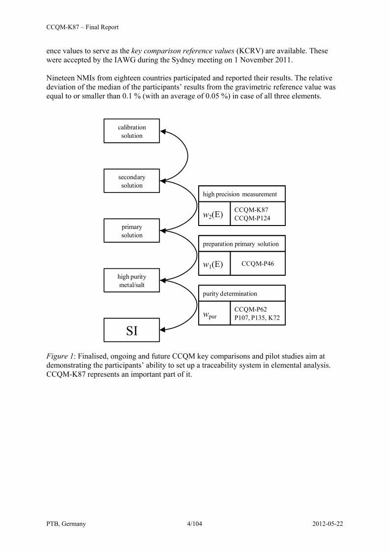
Traceability systems in elemental analysis [2] get their fundamental link to the SI via the pu-rity determination of suitable metals or salts. The demonstration of this capability was ad-dressed with CCQM-P62 (purity of Ni) [3] and CCQM-P107 (purity of Zn) [4]. And it is or will be the subject of ongoing or planned comparisons: CCQM-P135 (purity of NaCl) and CCQM-K72 (purity of Zn). The second link in the traceability chain – namely the primary solutions – was covered with CCQM-P46 (preparation of primary solutions of Cu, Mg and Rh). Linking all the measurements in the field to this system is crucial and usually achieved through calibration solutions, which was therefore decided to focus on in the framework of this key comparison (CCQM-K87) and the connected pilot study CCQM-P124. Three elements (chromium, cobalt and lead) were chosen to represent different kinds of needs and challenges. Chromium becomes increasingly important in environmental analysis. Cobalt as a mono-isotopic element cannot be determined using isotope dilution techniques. Lead usually requires the determination of the isotopic abundances in every sample because of its natural range of variation. Since the mass fractions of the three elements were adjusted gravimetrically and their original matrix contents were negligible compared to the adjusted content of 1 g/kg, gravimetric refer-
CCQM-K87 – Final Report
PTB, Germany 4/104 2012-05-22
ence values to serve as the key comparison reference values (KCRV) are available. These were accepted by the IAWG during the Sydney meeting on 1 November 2011. Nineteen NMIs from eighteen countries participated and reported their results. The relative deviation of the median of the participants’ results from the gravimetric reference value was equal to or smaller than 0.1 % (with an average of 0.05 %) in case of all three elements.
SI
calibrationsolution
secondarysolution
primarysolution
CCQM-P62P107, P135, K72wpur
purity determination
CCQM-P46w1(E)
preparation primary solution
CCQM-K87CCQM-P124w2(E)
high precision measurement
high purity metal/salt
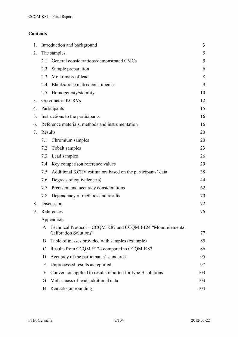
Figure 1: Finalised, ongoing and future CCQM key comparisons and pilot studies aim at demonstrating the participants’ ability to set up a traceability system in elemental analysis. CCQM-K87 represents an important part of it.
CCQM-K87 – Final Report
PTB, Germany 5/104 2012-05-22
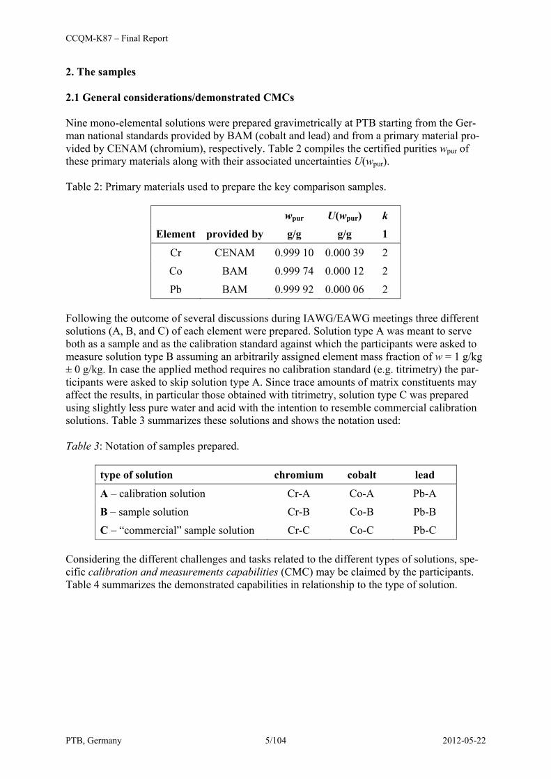
2. The samples 2.1 General considerations/demonstrated CMCs Nine mono-elemental solutions were prepared gravimetrically at PTB starting from the Ger-man national standards provided by BAM (cobalt and lead) and from a primary material pro-vided by CENAM (chromium), respectively. Table 2 compiles the certified purities wpur of these primary materials along with their associated uncertainties U(wpur). Table 2: Primary materials used to prepare the key comparison samples.
wpur U(wpur) k
Element provided by g/g g/g 1
Cr CENAM 0.999 10 0.000 39 2
Co BAM 0.999 74 0.000 12 2
Pb BAM 0.999 92 0.000 06 2 Following the outcome of several discussions during IAWG/EAWG meetings three different solutions (A, B, and C) of each element were prepared. Solution type A was meant to serve both as a sample and as the calibration standard against which the participants were asked to measure solution type B assuming an arbitrarily assigned element mass fraction of w = 1 g/kg ± 0 g/kg. In case the applied method requires no calibration standard (e.g. titrimetry) the par-ticipants were asked to skip solution type A. Since trace amounts of matrix constituents may affect the results, in particular those obtained with titrimetry, solution type C was prepared using slightly less pure water and acid with the intention to resemble commercial calibration solutions. Table 3 summarizes these solutions and shows the notation used: Table 3: Notation of samples prepared.
type of solution chromium cobalt lead
A – calibration solution Cr-A Co-A Pb-A
B – sample solution Cr-B Co-B Pb-B
C – “commercial” sample solution Cr-C Co-C Pb-C Considering the different challenges and tasks related to the different types of solutions, spe-cific calibration and measurements capabilities (CMC) may be claimed by the participants. Table 4 summarizes the demonstrated capabilities in relationship to the type of solution.
CCQM-K87 – Final Report
PTB, Germany 6/104 2012-05-22
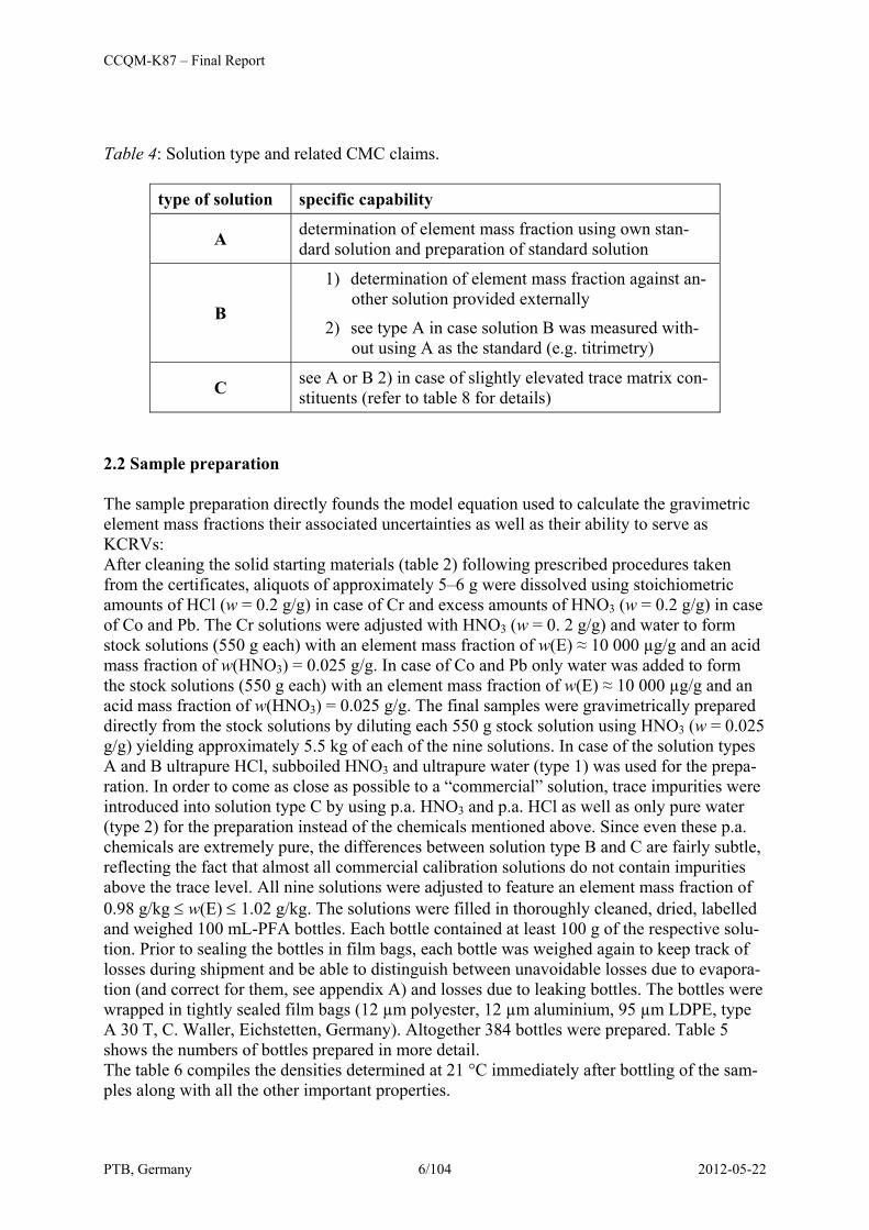
Table 4: Solution type and related CMC claims.
type of solution specific capability
A determination of element mass fraction using own stan-dard solution and preparation of standard solution
B
1) determination of element mass fraction against an-other solution provided externally
2) see type A in case solution B was measured with-out using A as the standard (e.g. titrimetry)
C see A or B 2) in case of slightly elevated trace matrix con-stituents (refer to table 8 for details)
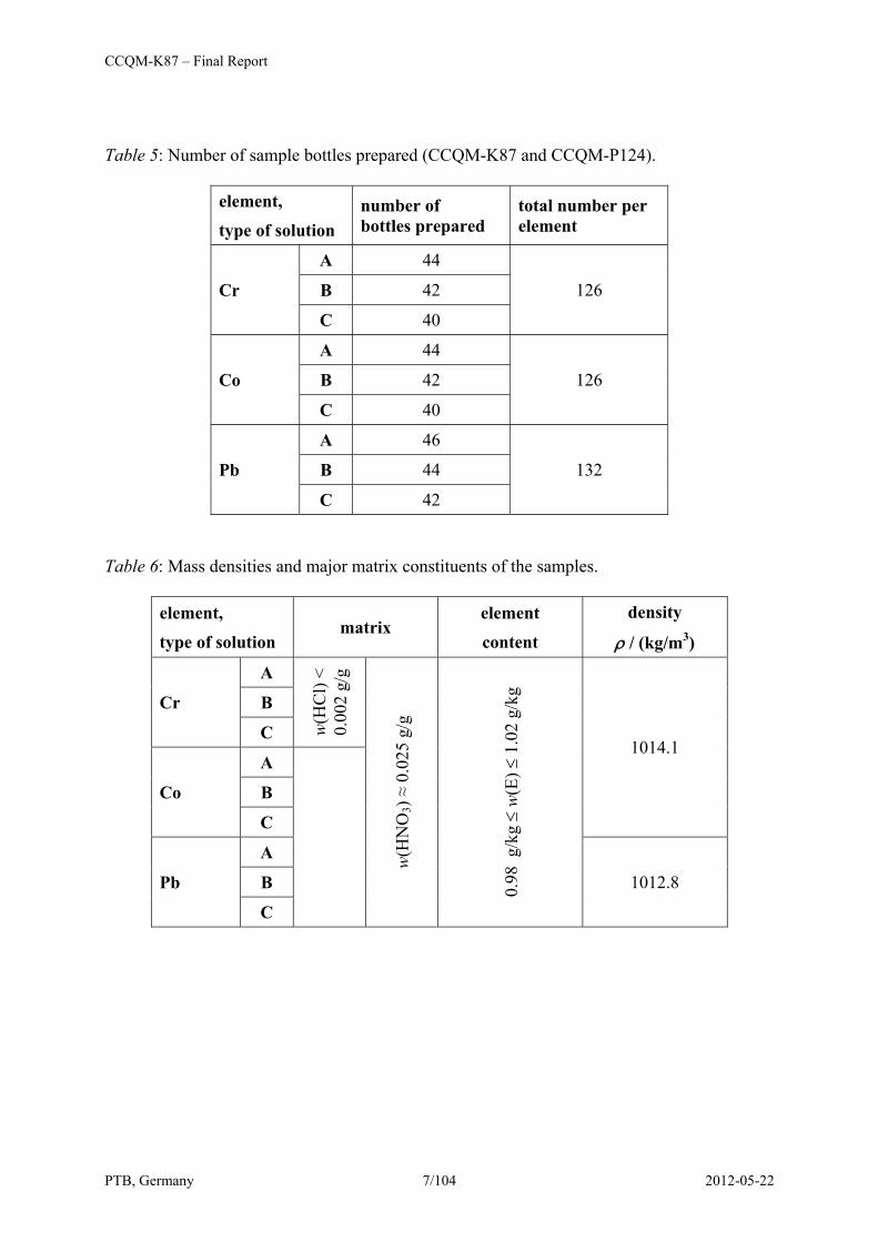
2.2 Sample preparation The sample preparation directly founds the model equation used to calculate the gravimetric element mass fractions their associated uncertainties as well as their ability to serve as KCRVs: After cleaning the solid starting materials (table 2) following prescribed procedures taken from the certificates, aliquots of approximately 5–6 g were dissolved using stoichiometric amounts of HCl (w = 0.2 g/g) in case of Cr and excess amounts of HNO3 (w = 0.2 g/g) in case of Co and Pb. The Cr solutions were adjusted with HNO3 (w = 0. 2 g/g) and water to form stock solutions (550 g each) with an element mass fraction of w(E) ≈ 10 000 µg/g and an acid mass fraction of w(HNO3) = 0.025 g/g. In case of Co and Pb only water was added to form the stock solutions (550 g each) with an element mass fraction of w(E) ≈ 10 000 µg/g and an acid mass fraction of w(HNO3) = 0.025 g/g. The final samples were gravimetrically prepared directly from the stock solutions by diluting each 550 g stock solution using HNO3 (w = 0.025 g/g) yielding approximately 5.5 kg of each of the nine solutions. In case of the solution types A and B ultrapure HCl, subboiled HNO3 and ultrapure water (type 1) was used for the prepa-ration. In order to come as close as possible to a “commercial” solution, trace impurities were introduced into solution type C by using p.a. HNO3 and p.a. HCl as well as only pure water (type 2) for the preparation instead of the chemicals mentioned above. Since even these p.a. chemicals are extremely pure, the differences between solution type B and C are fairly subtle, reflecting the fact that almost all commercial calibration solutions do not contain impurities above the trace level. All nine solutions were adjusted to feature an element mass fraction of 0.98 g/kg ≤ w(E) ≤ 1.02 g/kg. The solutions were filled in thoroughly cleaned, dried, labelled and weighed 100 mL-PFA bottles. Each bottle contained at least 100 g of the respective solu-tion. Prior to sealing the bottles in film bags, each bottle was weighed again to keep track of losses during shipment and be able to distinguish between unavoidable losses due to evapora-tion (and correct for them, see appendix A) and losses due to leaking bottles. The bottles were wrapped in tightly sealed film bags (12 µm polyester, 12 µm aluminium, 95 µm LDPE, type A 30 T, C. Waller, Eichstetten, Germany). Altogether 384 bottles were prepared. Table 5 shows the numbers of bottles prepared in more detail. The table 6 compiles the densities determined at 21 °C immediately after bottling of the sam-ples along with all the other important properties.
CCQM-K87 – Final Report
PTB, Germany 7/104 2012-05-22
Table 5: Number of sample bottles prepared (CCQM-K87 and CCQM-P124).
element,
type of solution number of bottles prepared
total number per element
Cr
A 44
126 B 42
C 40
Co
A 44
126 B 42
C 40
Pb
A 46
132 B 44
C 42 Table 6: Mass densities and major matrix constituents of the samples.
element,
type of solution matrix
element
content
density
ρ / (kg/m3)
Cr
A
w(H
Cl)
< 0.
002
g/g
w(H
NO
3) ≈
0.0
25 g
/g
0.98
g/k
g ≤
w(E
) ≤ 1
.02
g/kg
1014.1
B
C
Co
A
B
C
Pb
A
1012.8 B
C
CCQM-K87 – Final Report
PTB, Germany 8/104 2012-05-22
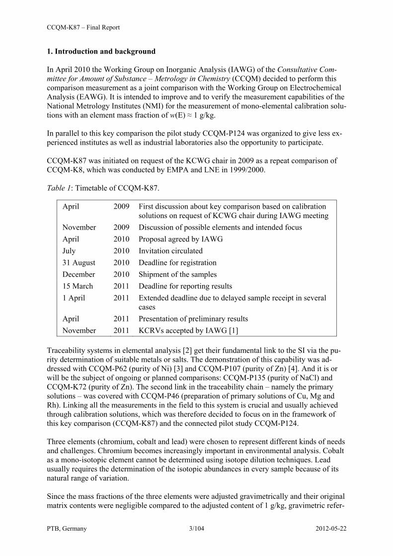
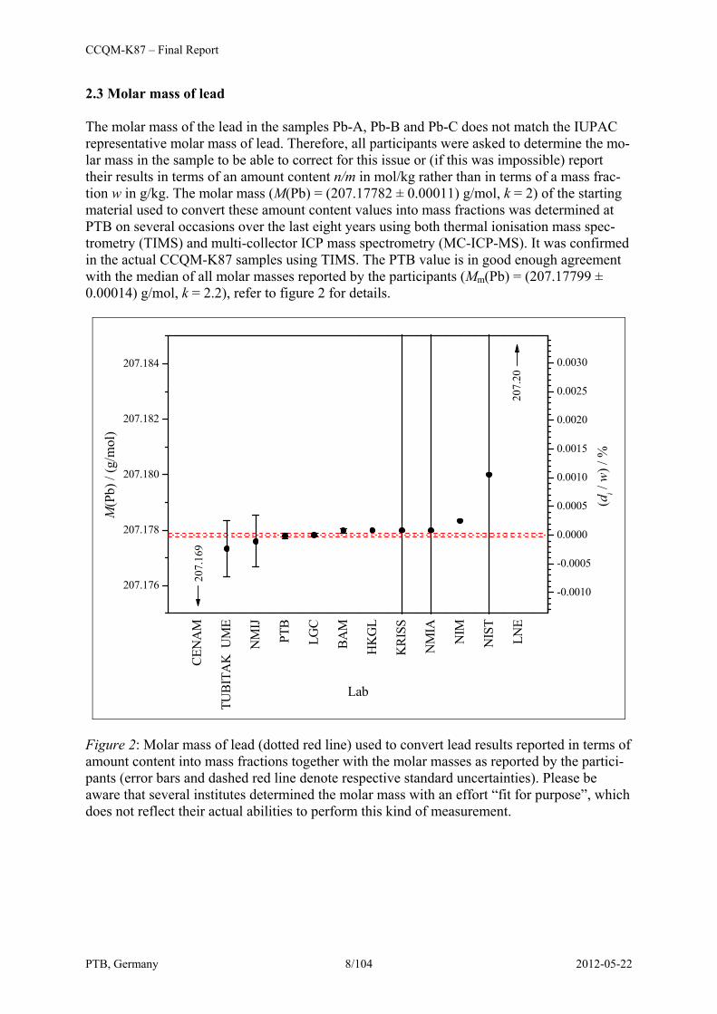
2.3 Molar mass of lead The molar mass of the lead in the samples Pb-A, Pb-B and Pb-C does not match the IUPAC representative molar mass of lead. Therefore, all participants were asked to determine the mo-lar mass in the sample to be able to correct for this issue or (if this was impossible) report their results in terms of an amount content n/m in mol/kg rather than in terms of a mass frac-tion w in g/kg. The molar mass (M(Pb) = (207.17782 ± 0.00011) g/mol, k = 2) of the starting material used to convert these amount content values into mass fractions was determined at PTB on several occasions over the last eight years using both thermal ionisation mass spec-trometry (TIMS) and multi-collector ICP mass spectrometry (MC-ICP-MS). It was confirmed in the actual CCQM-K87 samples using TIMS. The PTB value is in good enough agreement with the median of all molar masses reported by the participants (Mm(Pb) = (207.17799 ± 0.00014) g/mol, k = 2.2), refer to figure 2 for details.
CEN
AM
TUBI
TAK
UM
E
NM
IJ
PTB
LGC
BAM
HK
GL
KRI
SS
NM
IA
NIM
NIS
T
LNE
207.176
207.178
207.180
207.182
207.184
M(P
b) /
(g/m
ol)
Lab
207.
169
-0.0010
-0.0005
0.0000
0.0005
0.0010
0.0015
0.0020
0.0025
0.0030
(di /
w) /
%
207.
20
Figure 2: Molar mass of lead (dotted red line) used to convert lead results reported in terms of amount content into mass fractions together with the molar masses as reported by the partici-pants (error bars and dashed red line denote respective standard uncertainties). Please be aware that several institutes determined the molar mass with an effort “fit for purpose”, which does not reflect their actual abilities to perform this kind of measurement.
CCQM-K87 – Final Report
PTB, Germany 9/104 2012-05-22
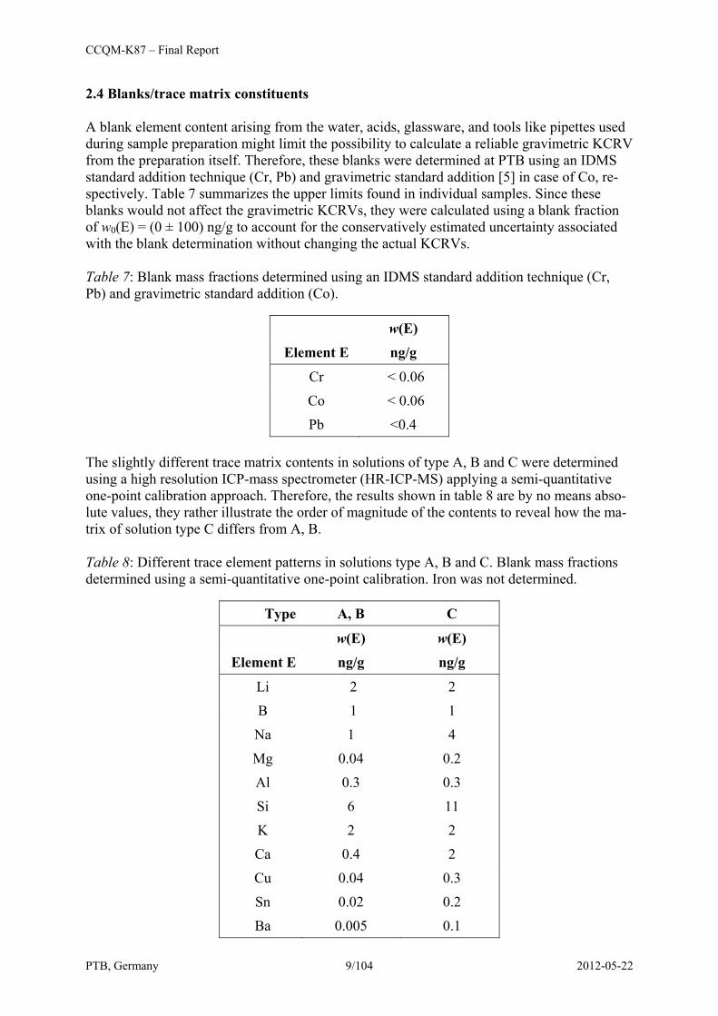
2.4 Blanks/trace matrix constituents A blank element content arising from the water, acids, glassware, and tools like pipettes used during sample preparation might limit the possibility to calculate a reliable gravimetric KCRV from the preparation itself. Therefore, these blanks were determined at PTB using an IDMS standard addition technique (Cr, Pb) and gravimetric standard addition [5] in case of Co, re-spectively. Table 7 summarizes the upper limits found in individual samples. Since these blanks would not affect the gravimetric KCRVs, they were calculated using a blank fraction of w0(E) = (0 ± 100) ng/g to account for the conservatively estimated uncertainty associated with the blank determination without changing the actual KCRVs. Table 7: Blank mass fractions determined using an IDMS standard addition technique (Cr, Pb) and gravimetric standard addition (Co).
w(E)
Element E ng/g
Cr < 0.06
Co < 0.06
Pb <0.4 The slightly different trace matrix contents in solutions of type A, B and C were determined using a high resolution ICP-mass spectrometer (HR-ICP-MS) applying a semi-quantitative one-point calibration approach. Therefore, the results shown in table 8 are by no means abso-lute values, they rather illustrate the order of magnitude of the contents to reveal how the ma-trix of solution type C differs from A, B. Table 8: Different trace element patterns in solutions type A, B and C. Blank mass fractions determined using a semi-quantitative one-point calibration. Iron was not determined.
Type A, B C
w(E) w(E)
Element E ng/g ng/g
Li 2 2
B 1 1
Na 1 4
Mg 0.04 0.2
Al 0.3 0.3
Si 6 11
K 2 2
Ca 0.4 2
Cu 0.04 0.3
Sn 0.02 0.2
Ba 0.005 0.1
CCQM-K87 – Final Report
PTB, Germany 10/104 2012-05-22
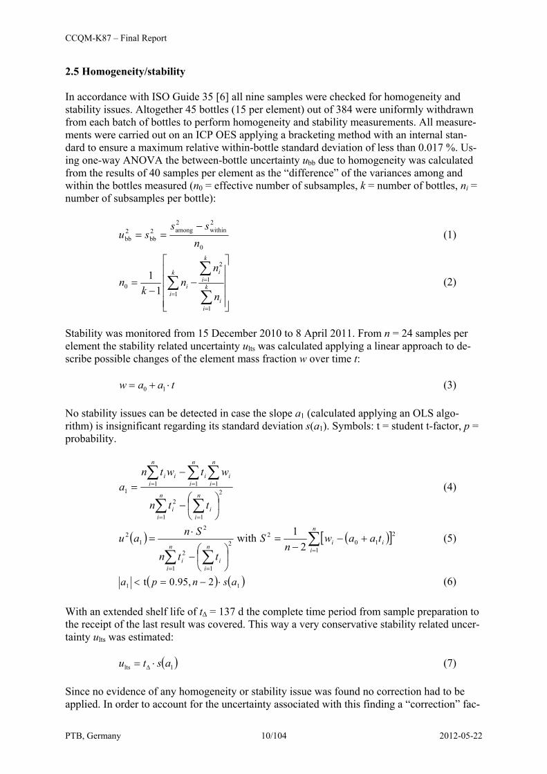
2.5 Homogeneity/stability In accordance with ISO Guide 35 [6] all nine samples were checked for homogeneity and stability issues. Altogether 45 bottles (15 per element) out of 384 were uniformly withdrawn from each batch of bottles to perform homogeneity and stability measurements. All measure-ments were carried out on an ICP OES applying a bracketing method with an internal stan-dard to ensure a maximum relative within-bottle standard deviation of less than 0.017 %. Us-ing one-way ANOVA the between-bottle uncertainty ubb due to homogeneity was calculated from the results of 40 samples per element as the “difference” of the variances among and within the bottles measured (n0 = effective number of subsamples, k = number of bottles, ni = number of subsamples per bottle):
0
2within
2among2
bb2bb n
sssu
−== (1)
⎥⎥⎥⎥
⎦
⎤
⎢⎢⎢⎢
⎣
⎡
−−
=
∑
∑∑
=
=
=k
ii
k
iik
ii
n
nn
kn
1
1
2
10 1
1 (2)
Stability was monitored from 15 December 2010 to 8 April 2011. From n = 24 samples per element the stability related uncertainty ults was calculated applying a linear approach to de-scribe possible changes of the element mass fraction w over time t: taaw ⋅+= 10 (3) No stability issues can be detected in case the slope a1 (calculated applying an OLS algo-rithm) is insignificant regarding its standard deviation s(a1). Symbols: t = student t-factor, p = probability.
2
11
2
1111
⎟⎠
⎞⎜⎝
⎛−
−=
∑∑
∑∑∑
==
===
n
ii
n
ii
n
ii
n
ii
n
iii
ttn
wtwtna (4)
( ) ( )[ ]∑∑∑
=
==
+−−
=
⎟⎠
⎞⎜⎝
⎛−
⋅=
n
iii
n
ii
n
ii
taawn
S
ttn
Snau1
210
22
11
2
2
12
21with (5)
( ) ( )11 2,95.0t asnpa ⋅−=< (6) With an extended shelf life of tΔ = 137 d the complete time period from sample preparation to the receipt of the last result was covered. This way a very conservative stability related uncer-tainty ults was estimated: ( )1lts astu ⋅= Δ (7) Since no evidence of any homogeneity or stability issue was found no correction had to be applied. In order to account for the uncertainty associated with this finding a “correction” fac-
CCQM-K87 – Final Report
PTB, Germany 11/104 2012-05-22
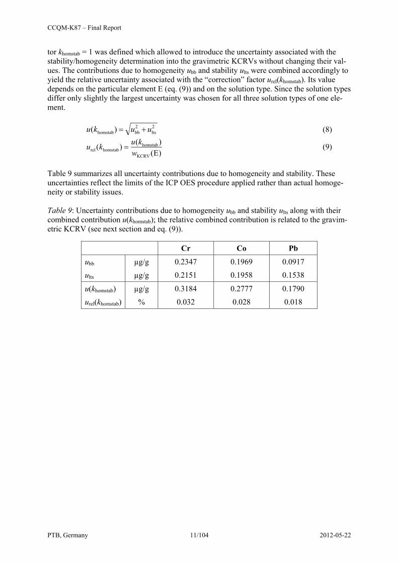
tor khomstab = 1 was defined which allowed to introduce the uncertainty associated with the stability/homogeneity determination into the gravimetric KCRVs without changing their val-ues. The contributions due to homogeneity ubb and stability ults were combined accordingly to yield the relative uncertainty associated with the “correction” factor urel(khomstab). Its value depends on the particular element E (eq. (9)) and on the solution type. Since the solution types differ only slightly the largest uncertainty was chosen for all three solution types of one ele-ment. 2
lts2bbhomstab)( uuku += (8)
)E()()(
KCRV
homstabhomstabrel w
kuku = (9)
Table 9 summarizes all uncertainty contributions due to homogeneity and stability. These uncertainties reflect the limits of the ICP OES procedure applied rather than actual homoge-neity or stability issues. Table 9: Uncertainty contributions due to homogeneity ubb and stability ults along with their combined contribution u(khomstab); the relative combined contribution is related to the gravim-etric KCRV (see next section and eq. (9)).
Cr Co Pb
ubb µg/g 0.2347 0.1969 0.0917
ults µg/g 0.2151 0.1958 0.1538
u(khomstab) µg/g 0.3184 0.2777 0.1790
urel(khomstab) % 0.032 0.028 0.018

CCQM-K87 – Final Report
PTB, Germany 12/104 2012-05-22
3. Gravimetric KCRVs The mass fraction wKCRV(E) of an element E was calculated as the sum of the added mass fraction wadd(E) plus the blank mass fraction w0(E) according to section 2.4 considering the homogeneity/stability contribution according section 2.5 yielding eq. (10): )E()E()E( 0addKCRV www += (10) The added element mass concentration wadd(E) was calculated from the preparation of the samples. A 5 L-borosilicate bottle was thoroughly cleaned, checked for the respective element E and dried. After weighing (m1r), an approximate volume of 4 L nitric acid (w(HNO3) = 0.025 g/g) was added. After weighing (m2r), approximately 0.5 kg of the primary reference solution (wz = w(E) ≈ 10 000 µg/g) was added. After weighing (m3r), another 0.8—1.2 L nitric acid (w(HNO3) = 0.025 g/g) was added (m4r) to adjust added element mass fractions of 0.98 g/kg ≤ wadd(E) ≤ 1.02 g/kg. Since all weighing steps had to be corrected for air buoyancy us-ing correction factors (Kij) taking into account the air density (air temperature, pressure and humidity) as well as the density of the sample (j) at any particular step (i) of the preparation procedure, the equation below was used to calculate the element mass fractions (KCRVs) wKCRV(E):
⎥⎥⎥⎥⎥
⎦
⎤
⎢⎢⎢⎢⎢
⎣
⎡
+
⎟⎟⎠
⎞⎜⎜⎝
⎛ ⋅−
⎥⎦
⎤⎢⎣
⎡⎟⎟⎠
⎞⎜⎜⎝
⎛ ⋅−−⎟⎟
⎠
⎞⎜⎜⎝
⎛ ⋅−
= )E()E( 0
BSG4
r1BSG1r44x
BSG2
r1BSG1r22NAc
BSG3
r1BSG1r33xz
homstabKCRV w
KmKmK
KmKmK
KmKmKw
kw (11)
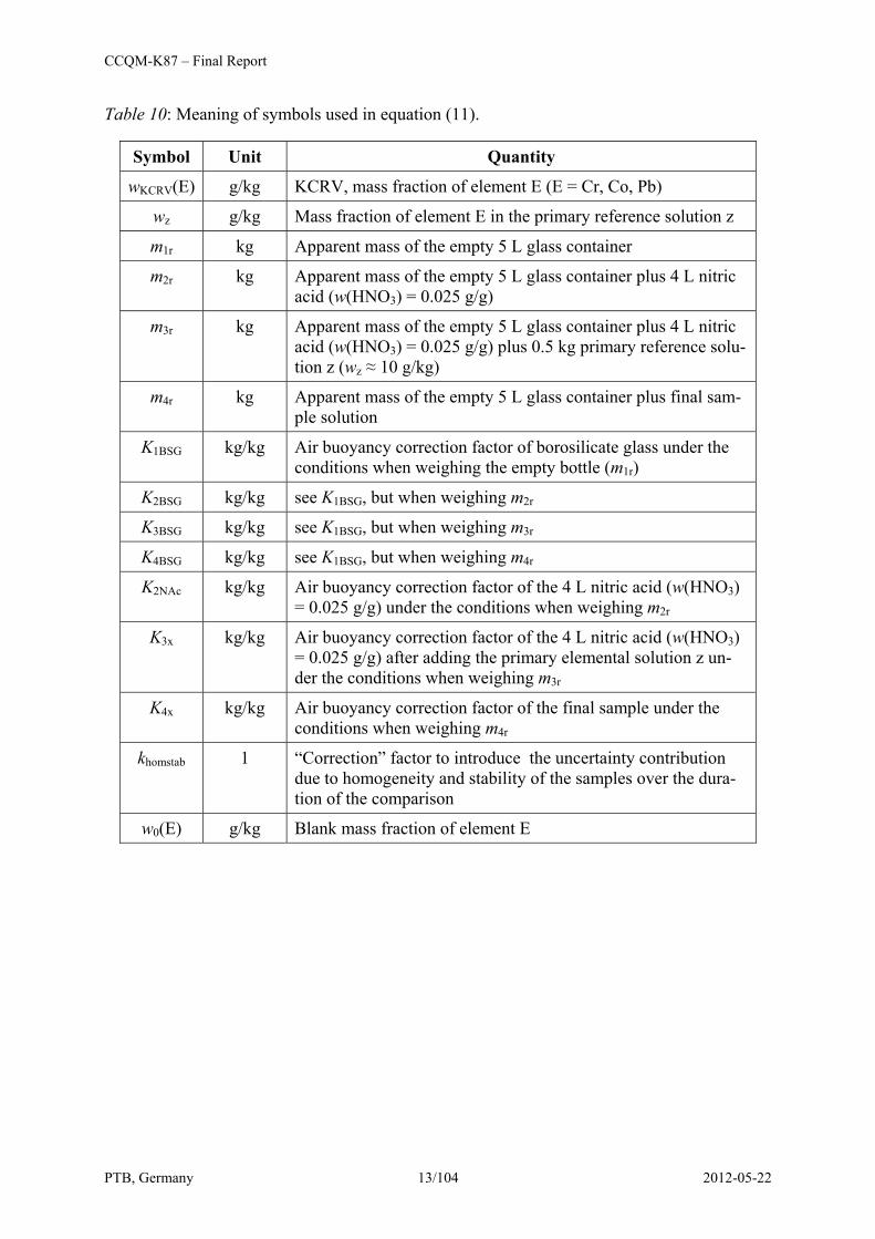
The blank mass fraction w0(E) was determined by PTB using a gravimetric standard addition technique combined with IDMS (Cr, Pb) and an internal standard (Co). Please refer to section 2.4 (table 7) for details. Equation (11) served as the model equation used to calculate the un-certainty associated with the KCRVs (meaning of the symbols used are compiled in table 10) in accordance with [7]. No significant homogeneity or stability issues were determined within the reproducibility of the ICP OES method applied. The factor khomstab featuring a value of one accounts for this limitation with its associated uncertainty. Please refer to section 2.5 for de-tails.
CCQM-K87 – Final Report
PTB, Germany 13/104 2012-05-22
Table 10: Meaning of symbols used in equation (11).
Symbol Unit Quantity
wKCRV(E) g/kg KCRV, mass fraction of element E (E = Cr, Co, Pb)
wz g/kg Mass fraction of element E in the primary reference solution z
m1r kg Apparent mass of the empty 5 L glass container
m2r kg Apparent mass of the empty 5 L glass container plus 4 L nitric acid (w(HNO3) = 0.025 g/g)
m3r kg Apparent mass of the empty 5 L glass container plus 4 L nitric acid (w(HNO3) = 0.025 g/g) plus 0.5 kg primary reference solu-tion z (wz ≈ 10 g/kg)
m4r kg Apparent mass of the empty 5 L glass container plus final sam-ple solution
K1BSG kg/kg Air buoyancy correction factor of borosilicate glass under the conditions when weighing the empty bottle (m1r)
K2BSG kg/kg see K1BSG, but when weighing m2r
K3BSG kg/kg see K1BSG, but when weighing m3r
K4BSG kg/kg see K1BSG, but when weighing m4r
K2NAc kg/kg Air buoyancy correction factor of the 4 L nitric acid (w(HNO3) = 0.025 g/g) under the conditions when weighing m2r
K3x kg/kg Air buoyancy correction factor of the 4 L nitric acid (w(HNO3) = 0.025 g/g) after adding the primary elemental solution z un-der the conditions when weighing m3r
K4x kg/kg Air buoyancy correction factor of the final sample under the conditions when weighing m4r
khomstab 1 “Correction” factor to introduce the uncertainty contribution due to homogeneity and stability of the samples over the dura-tion of the comparison
w0(E) g/kg Blank mass fraction of element E
CCQM-K87 – Final Report
PTB, Germany 14/104 2012-05-22
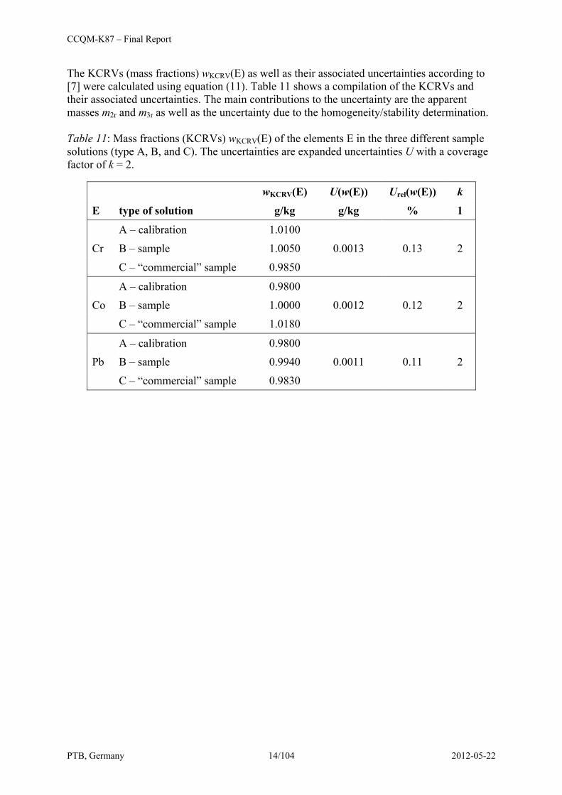
The KCRVs (mass fractions) wKCRV(E) as well as their associated uncertainties according to [7] were calculated using equation (11). Table 11 shows a compilation of the KCRVs and their associated uncertainties. The main contributions to the uncertainty are the apparent masses m2r and m3r as well as the uncertainty due to the homogeneity/stability determination. Table 11: Mass fractions (KCRVs) wKCRV(E) of the elements E in the three different sample solutions (type A, B, and C). The uncertainties are expanded uncertainties U with a coverage factor of k = 2.
wKCRV(E) U(w(E)) Urel(w(E)) k
E type of solution g/kg g/kg % 1
Cr
A – calibration 1.0100
0.0013 0.13 2 B – sample 1.0050
C – “commercial” sample 0.9850
Co
A – calibration 0.9800
0.0012 0.12 2 B – sample 1.0000
C – “commercial” sample 1.0180
Pb
A – calibration 0.9800
0.0011 0.11 2 B – sample 0.9940
C – “commercial” sample 0.9830
CCQM-K87 – Final Report
PTB, Germany 15/104 2012-05-22
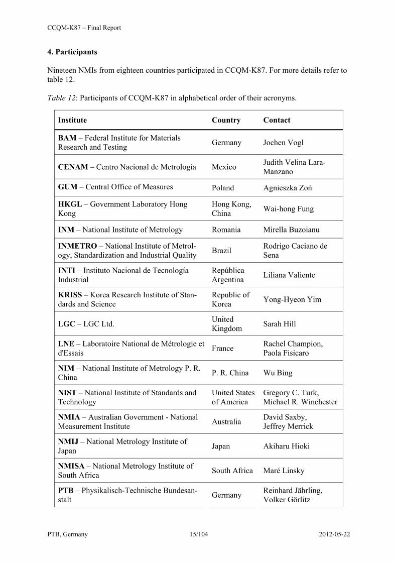
4. Participants Nineteen NMIs from eighteen countries participated in CCQM-K87. For more details refer to table 12. Table 12: Participants of CCQM-K87 in alphabetical order of their acronyms.
Institute Country Contact
BAM – Federal Institute for Materials Research and Testing Germany Jochen Vogl
CENAM – Centro Nacional de Metrología Mexico Judith Velina Lara-Manzano
GUM – Central Office of Measures Poland Agnieszka Zoń
HKGL – Government Laboratory Hong Kong
Hong Kong, China Wai-hong Fung
INM – National Institute of Metrology Romania Mirella Buzoianu
INMETRO – National Institute of Metrol-ogy, Standardization and Industrial Quality Brazil Rodrigo Caciano de
Sena
INTI – Instituto Nacional de Tecnología Industrial
República Argentina Liliana Valiente
KRISS – Korea Research Institute of Stan-dards and Science
Republic of Korea Yong-Hyeon Yim
LGC – LGC Ltd. United Kingdom Sarah Hill
LNE – Laboratoire National de Métrologie et d'Essais France Rachel Champion,
Paola Fisicaro
NIM – National Institute of Metrology P. R. China P. R. China Wu Bing
NIST – National Institute of Standards and Technology
United States of America
Gregory C. Turk, Michael R. Winchester
NMIA – Australian Government - National Measurement Institute Australia David Saxby,
Jeffrey Merrick
NMIJ – National Metrology Institute of Japan Japan Akiharu Hioki
NMISA – National Metrology Institute of South Africa South Africa Maré Linsky
PTB – Physikalisch-Technische Bundesan-stalt Germany Reinhard Jährling,
Volker Görlitz
CCQM-K87 – Final Report
PTB, Germany 16/104 2012-05-22
Institute Country Contact
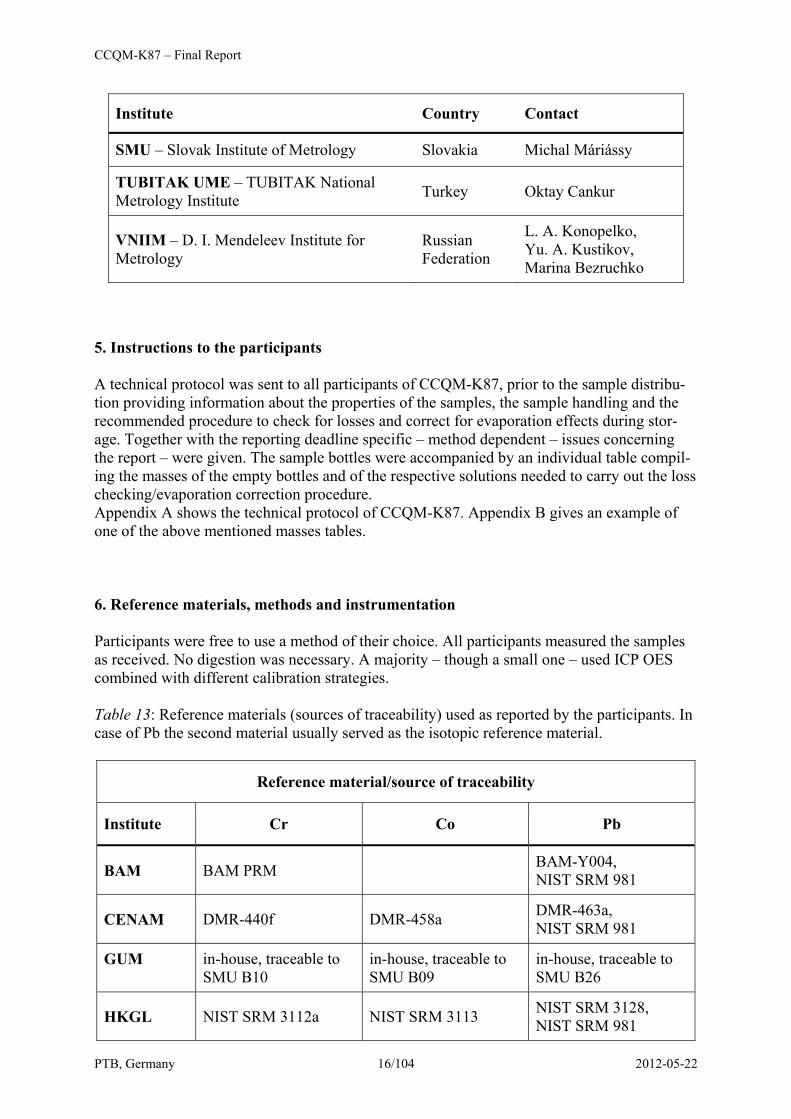
SMU – Slovak Institute of Metrology Slovakia Michal Máriássy
TUBITAK UME – TUBITAK National Metrology Institute Turkey Oktay Cankur
VNIIM – D. I. Mendeleev Institute for Metrology
Russian Federation
L. A. Konopelko, Yu. A. Kustikov, Marina Bezruchko
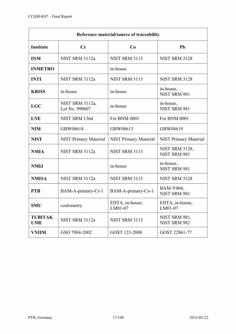
5. Instructions to the participants A technical protocol was sent to all participants of CCQM-K87, prior to the sample distribu-tion providing information about the properties of the samples, the sample handling and the recommended procedure to check for losses and correct for evaporation effects during stor-age. Together with the reporting deadline specific – method dependent – issues concerning the report – were given. The sample bottles were accompanied by an individual table compil-ing the masses of the empty bottles and of the respective solutions needed to carry out the loss checking/evaporation correction procedure. Appendix A shows the technical protocol of CCQM-K87. Appendix B gives an example of one of the above mentioned masses tables. 6. Reference materials, methods and instrumentation Participants were free to use a method of their choice. All participants measured the samples as received. No digestion was necessary. A majority – though a small one – used ICP OES combined with different calibration strategies. Table 13: Reference materials (sources of traceability) used as reported by the participants. In case of Pb the second material usually served as the isotopic reference material.
Reference material/source of traceability
Institute Cr Co Pb
BAM BAM PRM BAM-Y004, NIST SRM 981
CENAM DMR-440f DMR-458a DMR-463a, NIST SRM 981
GUM in-house, traceable to SMU B10
in-house, traceable to SMU B09
in-house, traceable to SMU B26
HKGL NIST SRM 3112a NIST SRM 3113 NIST SRM 3128, NIST SRM 981
CCQM-K87 – Final Report
PTB, Germany 17/104 2012-05-22
Reference material/source of traceability
Institute Cr Co Pb
INM NIST SRM 3112a NIST SRM 3113 NIST SRM 3128
INMETRO in-house
INTI NIST SRM 3112a NIST SRM 3113 NIST SRM 3128
KRISS in-house in-house in-house, NIST SRM 981
LGC NIST SRM 3112a, Lot No. 990607 in-house in-house,
NIST SRM 981
LNE NIST SRM 136d Fer BNM 0001 Fer BNM 0001
NIM GBW08614 GBW08613 GBW08619
NIST NIST Primary Material NIST Primary Material NIST Primary Material
NMIA NIST SRM 3112a NIST SRM 3113 NIST SRM 3128, NIST SRM 981
NMIJ in-house in-house, NIST SRM 981
NMISA NIST SRM 3112a NIST SRM 3113 NIST SRM 3128
PTB BAM-A-primary-Cr-1 BAM-A-primary-Co-1 BAM-Y004, NIST SRM 981
SMU coulometry EDTA, in-house, LM01-07
EDTA, in-house, LM01-07
TUBITAK UME NIST SRM 3112a NIST SRM 3113 NIST SRM 981,
NIST SRM 982
VNIIM GSO 7984-2002 GOST 123-2008 GOST 22861-77

CCQM-K87 – Final Report
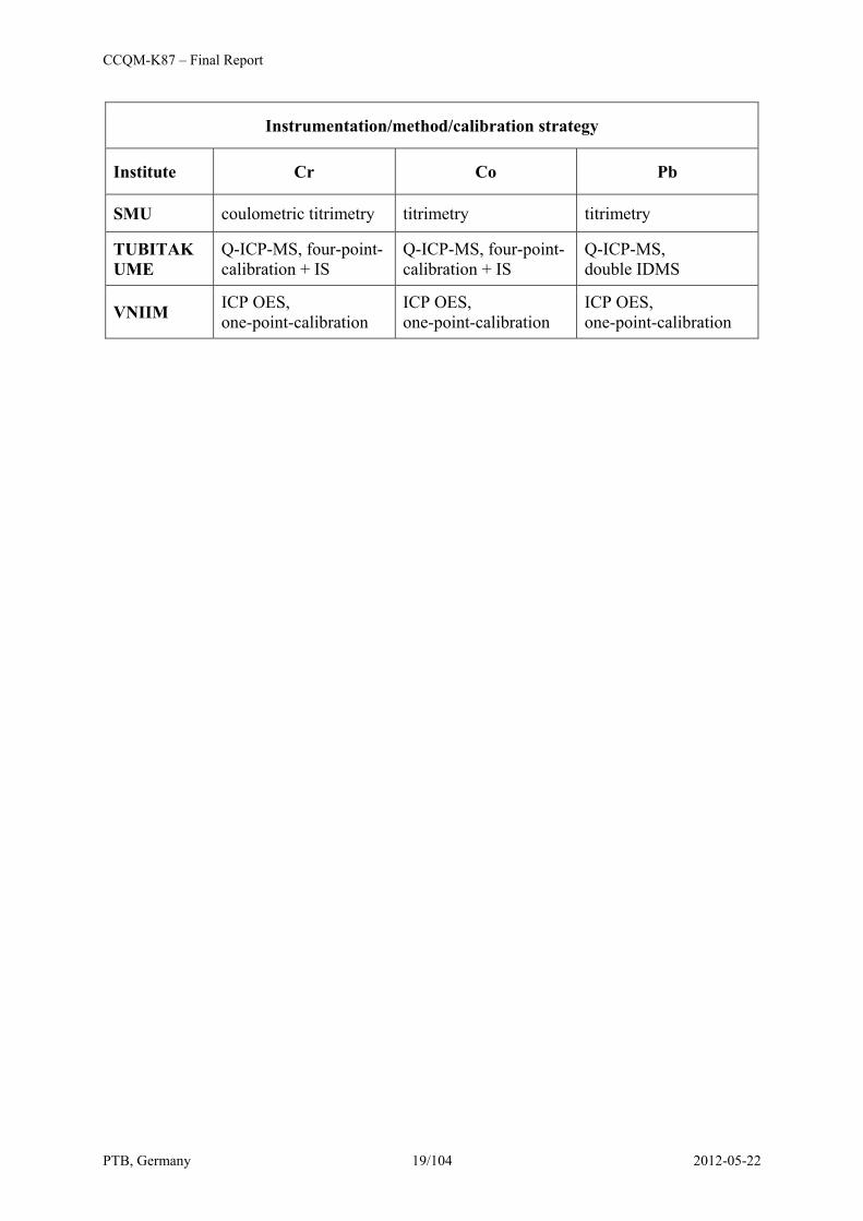
PTB, Germany 18/104 2012-05-22
Table 14: Instrumentation/method and calibration strategy used as reported by the participants (IS = internal standard).
Instrumentation/method/calibration strategy
Institute Cr Co Pb
BAM MC-TIMS, double IDMS MC-TIMS,
double IDMS
CENAM-1 ICP OES, one-point-calibration + IS
ICP OES, one-point-calibration + IS
ICP OES, one-point-calibration + IS
CENAM-2 titrimetry
GUM ICP OES, one-point-calibration
ICP OES, one-point-calibration
ICP OES, one-point-calibration
HKGL ICP OES, one-point-calibration + IS
ICP OES, one-point-calibration + IS
ICP OES, one-point-calibration + IS
INM Q-ICP-MS, calibration curve
Q-ICP-MS, calibration curve
Q-ICP-MS, calibration curve
INMETRO ICP OES, calibration curve
INTI FAAS, one-point-calibration
ICP OES, one-point-calibration
FAAS, one-point-calibration
KRISS ICP OES, one-point-calibration + IS
ICP OES, one-point-calibration + IS
ICP OES, one-point-calibration + IS
LGC MC-ICP-MS, double IDMS
Q-ICP-MS, one-point-calibration + IS
MC-ICP-MS, double IDMS
LNE Q-ICP-MS, double IDMS titrimetry titrimetry
NIM Q-ICP-MS, bracketing + IS
Q-ICP-MS, bracketing + IS
Q-ICP-MS, bracketing + IS
NIST ICP OES, one-point-calibration + IS
ICP OES, one-point-calibration + IS
ICP OES, one-point-calibration + IS
NMIA HR-ICP-MS, double IDMS
HR-ICP-MS, one-point-calibration + IS
HR-ICP-MS, double IDMS
NMIJ titrimetry titrimetry
NMISA ICP OES, bracketing + IS
ICP OES, bracketing + IS
ICP OES, bracketing + IS
PTB ICP OES, bracketing + IS
ICP OES, bracketing + IS
ICP OES, bracketing + IS
CCQM-K87 – Final Report
PTB, Germany 19/104 2012-05-22
Instrumentation/method/calibration strategy
Institute Cr Co Pb
SMU coulometric titrimetry titrimetry titrimetry
TUBITAK UME
Q-ICP-MS, four-point-calibration + IS
Q-ICP-MS, four-point-calibration + IS
Q-ICP-MS, double IDMS
VNIIM ICP OES, one-point-calibration
ICP OES, one-point-calibration
ICP OES, one-point-calibration
CCQM-K87 – Final Report
PTB, Germany 20/104 2012-05-22
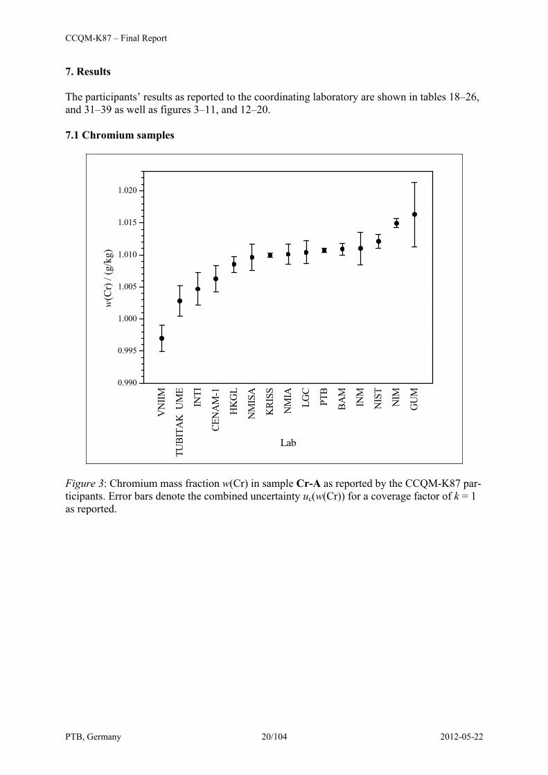
7. Results The participants’ results as reported to the coordinating laboratory are shown in tables 18–26, and 31–39 as well as figures 3–11, and 12–20. 7.1 Chromium samples
VN
IIM
TUBI
TAK
UM
E
INTI
CEN
AM
-1
HK
GL
NM
ISA
KRI
SS
NM
IA
LGC
PTB
BAM
INM
NIS
T
NIM
GU
M
0.990
0.995
1.000
1.005
1.010
1.015
1.020
w(C
r) /
(g/k
g)
Lab
Figure 3: Chromium mass fraction w(Cr) in sample Cr-A as reported by the CCQM-K87 par-ticipants. Error bars denote the combined uncertainty uc(w(Cr)) for a coverage factor of k = 1 as reported.
CCQM-K87 – Final Report
PTB, Germany 21/104 2012-05-22
TUBI
TAK
UM
EN
MIA
SMU
LGC
KRI
SSH
KG
LPT
BCE
NA
M-1
BAM
NM
ISA
GU
MN
IST
NIM
INTI
INM
LNE
VN
IIM
0.995
1.000
1.005
1.010
1.015w
(Cr)
/ (g
/kg)
Lab
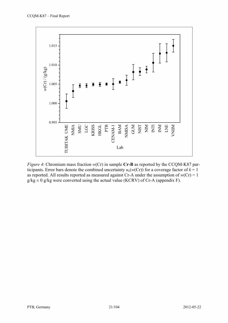
Figure 4: Chromium mass fraction w(Cr) in sample Cr-B as reported by the CCQM-K87 par-ticipants. Error bars denote the combined uncertainty uc(w(Cr)) for a coverage factor of k = 1 as reported. All results reported as measured against Cr-A under the assumption of w(Cr) = 1 g/kg ± 0 g/kg were converted using the actual value (KCRV) of Cr-A (appendix F).
CCQM-K87 – Final Report
PTB, Germany 22/104 2012-05-22
TUBI
TAK
UM
E
CEN
AM
-1
SMU
KRI
SS
NM
IA
NM
ISA
INTI
PTB
BAM
NIS
T
NIM
GU
M
LNE
VN
IIM
0.975
0.980
0.985
0.990
0.995
1.000
w(C
r) /
(g/k
g)
Lab
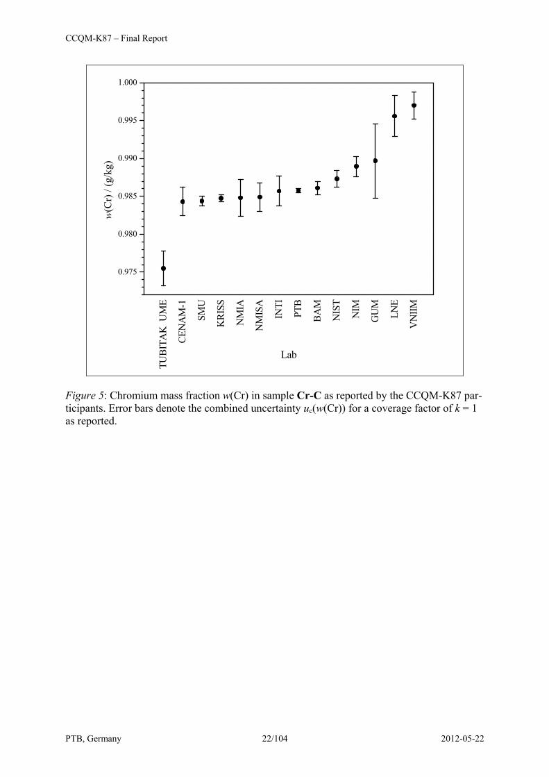
Figure 5: Chromium mass fraction w(Cr) in sample Cr-C as reported by the CCQM-K87 par-ticipants. Error bars denote the combined uncertainty uc(w(Cr)) for a coverage factor of k = 1 as reported.
CCQM-K87 – Final Report
PTB, Germany 23/104 2012-05-22
7.2 Cobalt samples
NM
IA
NIM PT
B
CEN
AM
-1
NM
IJ
KRI
SS
NIS
T
NM
ISA
HK
GL
GU
M
TUBI
TAK
UM
E
INM
ETRO INTI
LGC
INM
VN
IIM
0.975
0.980
0.985
0.990
0.995
1.000
1.005
1.010w
(Co)
/ (g
/kg)
Lab
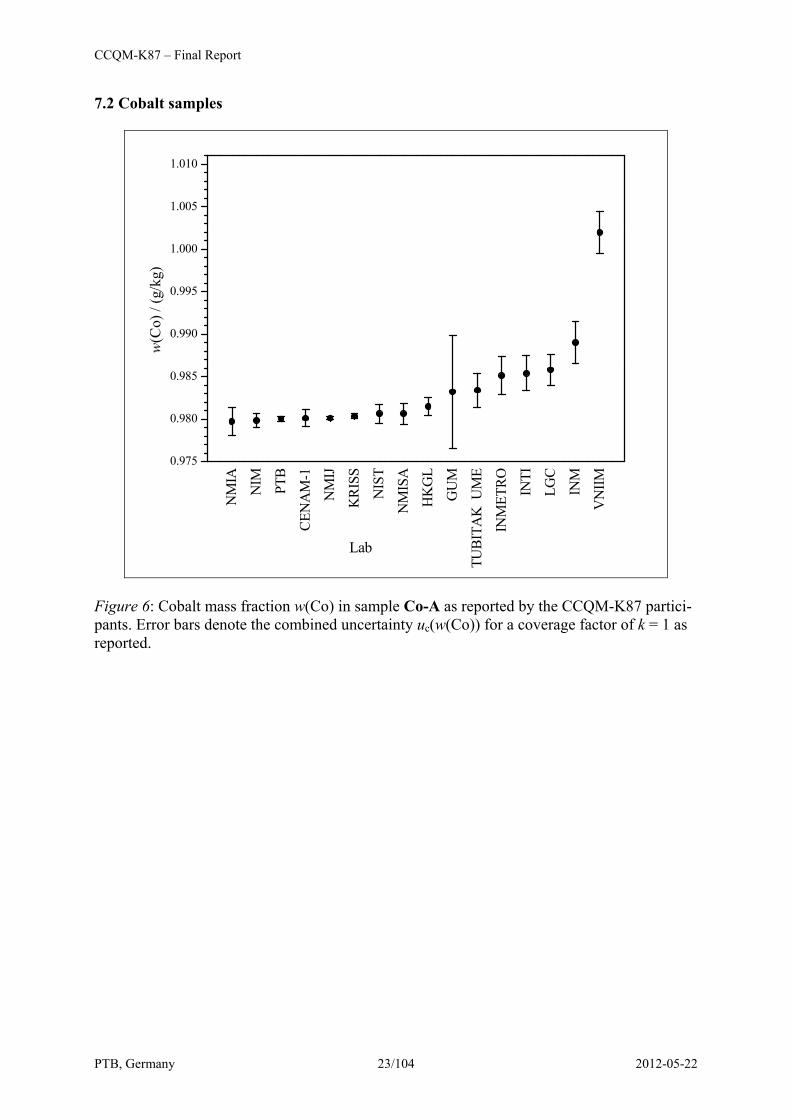
Figure 6: Cobalt mass fraction w(Co) in sample Co-A as reported by the CCQM-K87 partici-pants. Error bars denote the combined uncertainty uc(w(Co)) for a coverage factor of k = 1 as reported.
CCQM-K87 – Final Report
PTB, Germany 24/104 2012-05-22
INTI
VN
IIM INM
GU
MIN
MET
RO NIM
TUBI
TAK
UM
EN
MIS
AN
MIA
LNE
HK
GL
NM
IJK
RISS
CEN
AM
-1SM
UPT
BLG
CN
IST
0.985
0.990
0.995
1.000
1.005
w(C
o) /
(g/k
g)
Lab
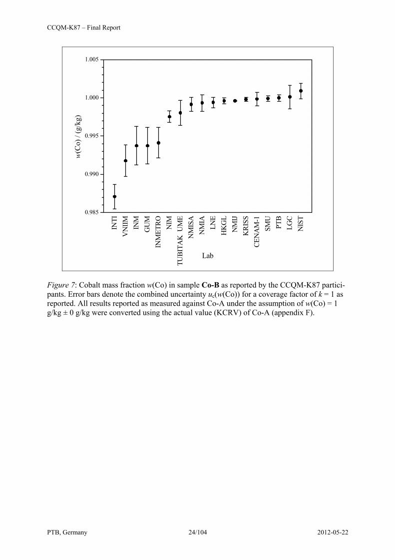
Figure 7: Cobalt mass fraction w(Co) in sample Co-B as reported by the CCQM-K87 partici-pants. Error bars denote the combined uncertainty uc(w(Co)) for a coverage factor of k = 1 as reported. All results reported as measured against Co-A under the assumption of w(Co) = 1 g/kg ± 0 g/kg were converted using the actual value (KCRV) of Co-A (appendix F).
CCQM-K87 – Final Report
PTB, Germany 25/104 2012-05-22
VN
IIM INTI
TUBI
TAK
UM
E
NIM
LNE
CEN
AM
-1
NM
ISA
KRI
SS
NM
IJ
PTB
SMU
GU
M
INM
ETRO
NIS
T
NM
IA
0.995
1.000
1.005
1.010
1.015
1.020
1.025w
(Co)
/ (g
/kg)
Lab
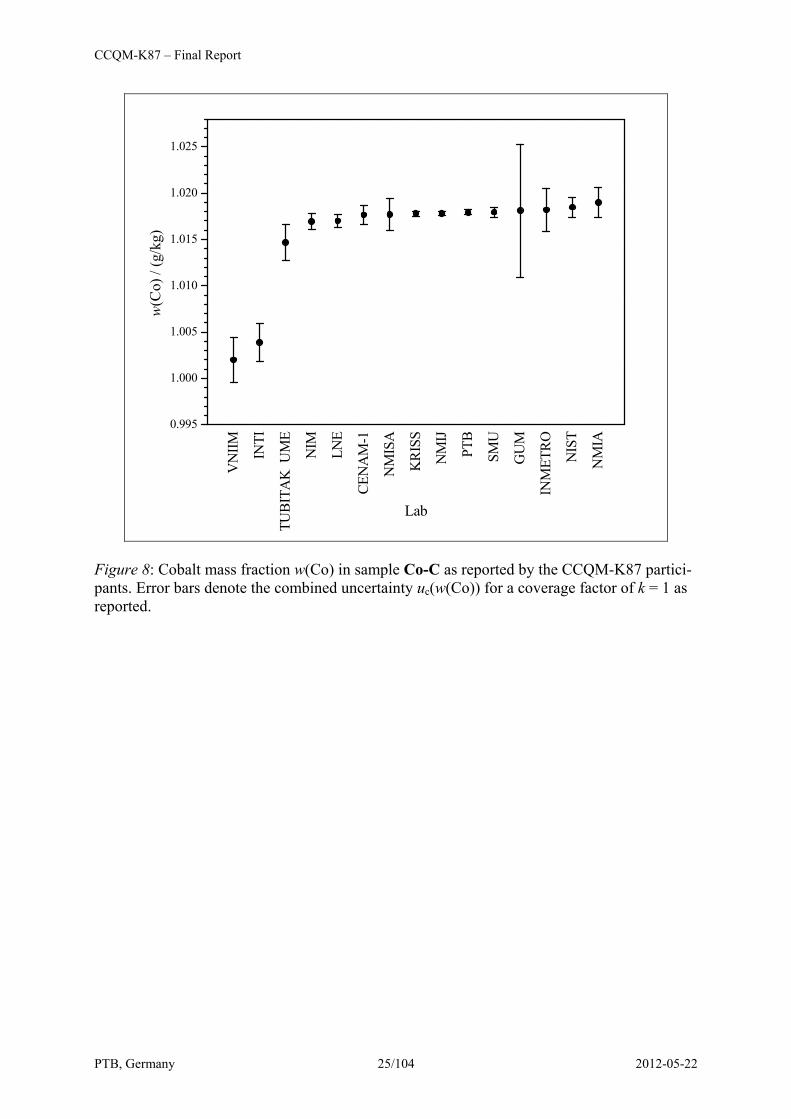
Figure 8: Cobalt mass fraction w(Co) in sample Co-C as reported by the CCQM-K87 partici-pants. Error bars denote the combined uncertainty uc(w(Co)) for a coverage factor of k = 1 as reported.
CCQM-K87 – Final Report
PTB, Germany 26/104 2012-05-22
7.3 Lead samples
BAM
NM
IJ
PTB
LGC
NIM
KRI
SS
CEN
AM
-1
HK
GL
NIS
T
NM
IA
NM
ISA
INM
TUBI
TAK
UM
E
VN
IIM INTI
GU
M
0.975
0.980
0.985
0.990
0.995
1.000
1.005
1.010
1.03
59
w(P
b) /
(g/k
g)
Lab
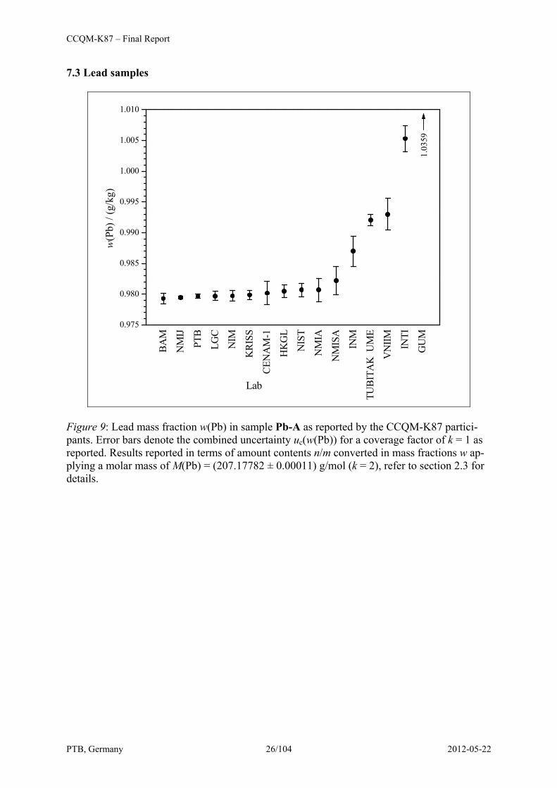
Figure 9: Lead mass fraction w(Pb) in sample Pb-A as reported by the CCQM-K87 partici-pants. Error bars denote the combined uncertainty uc(w(Pb)) for a coverage factor of k = 1 as reported. Results reported in terms of amount contents n/m converted in mass fractions w ap-plying a molar mass of M(Pb) = (207.17782 ± 0.00011) g/mol (k = 2), refer to section 2.3 for details.
CCQM-K87 – Final Report
PTB, Germany 27/104 2012-05-22
INTI
TUBI
TAK
UM
EN
MIA
CEN
AM
-2N
IST
HK
GL
KRI
SSPT
BLG
CSM
UBA
MCE
NA
M-1
NM
IJIN
MN
IMG
UM
LNE
NM
ISA
VN
IIM
0.985
0.990
0.995
1.000w
(Pb)
/ (g
/kg)
Lab
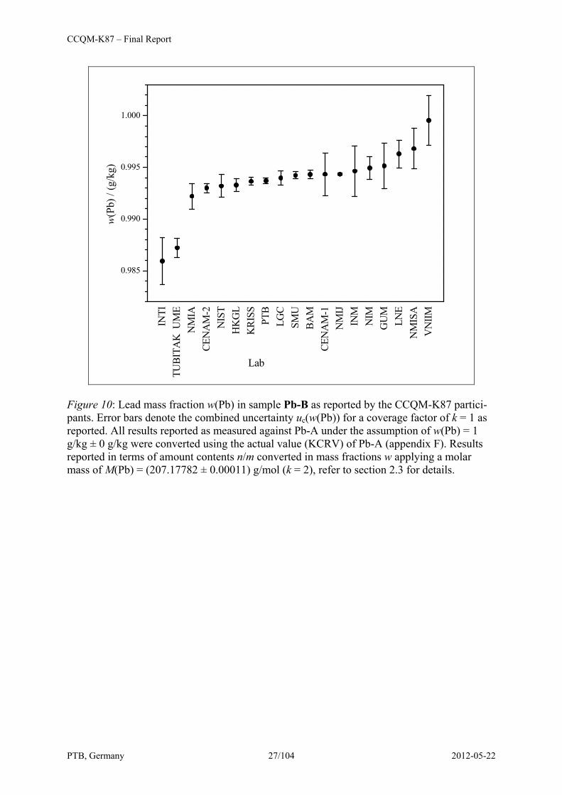
Figure 10: Lead mass fraction w(Pb) in sample Pb-B as reported by the CCQM-K87 partici-pants. Error bars denote the combined uncertainty uc(w(Pb)) for a coverage factor of k = 1 as reported. All results reported as measured against Pb-A under the assumption of w(Pb) = 1 g/kg ± 0 g/kg were converted using the actual value (KCRV) of Pb-A (appendix F). Results reported in terms of amount contents n/m converted in mass fractions w applying a molar mass of M(Pb) = (207.17782 ± 0.00011) g/mol (k = 2), refer to section 2.3 for details.
CCQM-K87 – Final Report
PTB, Germany 28/104 2012-05-22
NM
ISA
NM
IA
BAM
NIM
KRI
SS
NM
IJ
PTB
SMU
CEN
AM
-1
NIS
T
CEN
AM
-2
LNE
TUBI
TAK
UM
E
INTI
VN
IIM
GU
M
0.975
0.980
0.985
0.990
0.995
1.000
w(P
b) /
(g/k
g)
Lab
1.03
80
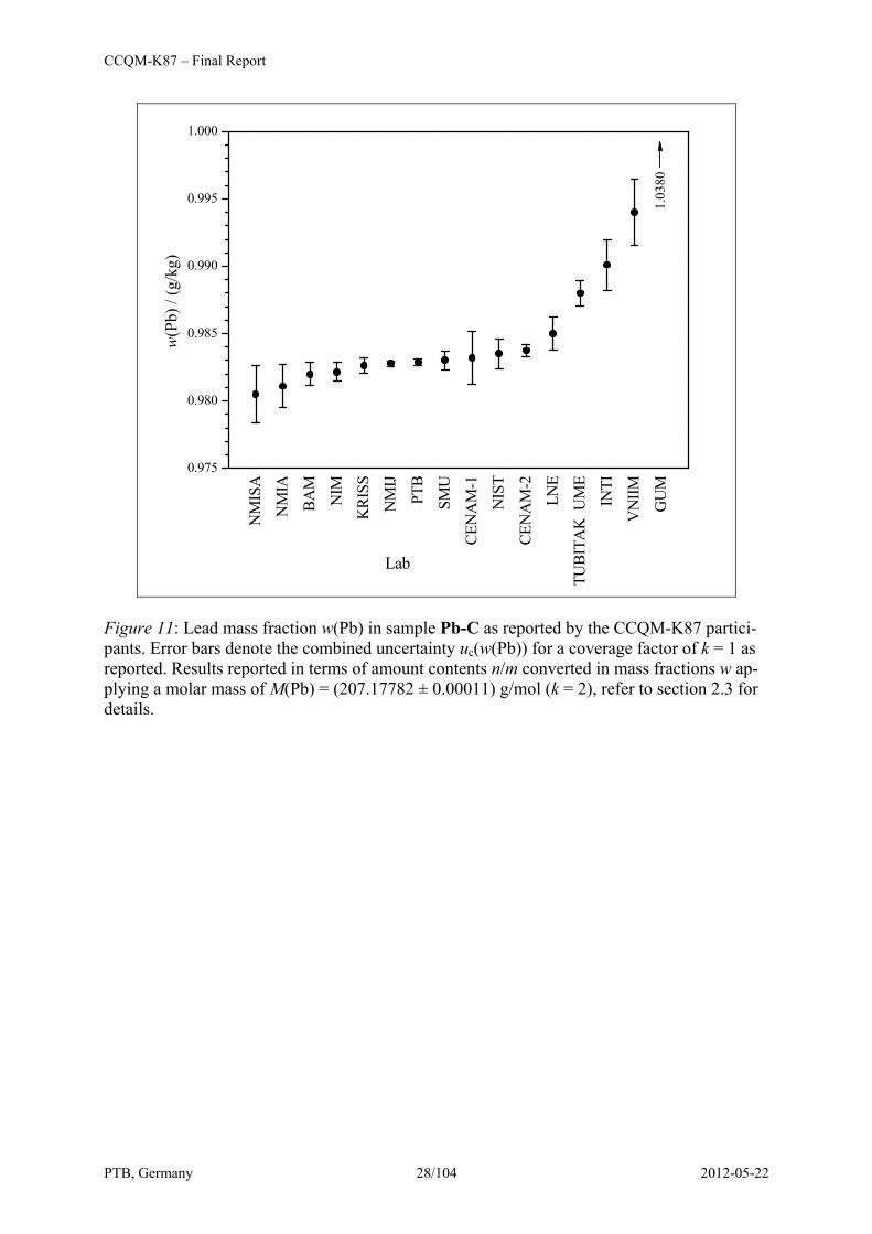
Figure 11: Lead mass fraction w(Pb) in sample Pb-C as reported by the CCQM-K87 partici-pants. Error bars denote the combined uncertainty uc(w(Pb)) for a coverage factor of k = 1 as reported. Results reported in terms of amount contents n/m converted in mass fractions w ap-plying a molar mass of M(Pb) = (207.17782 ± 0.00011) g/mol (k = 2), refer to section 2.3 for details.
CCQM-K87 – Final Report
PTB, Germany 29/104 2012-05-22
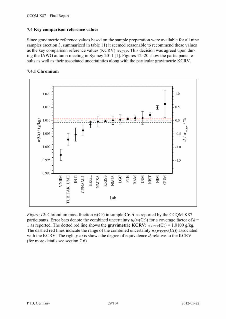
7.4 Key comparison reference values Since gravimetric reference values based on the sample preparation were available for all nine samples (section 3, summarized in table 11) it seemed reasonable to recommend these values as the key comparison reference values (KCRV) wKCRV. This decision was agreed upon dur-ing the IAWG autumn meeting in Sydney 2011 [1]. Figures 12–20 show the participants re-sults as well as their associated uncertainties along with the particular gravimetric KCRV. 7.4.1 Chromium
VN
IIM
TUBI
TAK
UM
E
INTI
CEN
AM
-1
HK
GL
NM
ISA
KRI
SS
NM
IA
LGC
PTB
BAM
INM
NIS
T
NIM
GU
M
0.990
0.995
1.000
1.005
1.010
1.015
1.020
w(C
r) /
(g/k
g)
Lab
-1.5
-1.0
-0.5
0.0
0.5
1.0
di /
wK
CR
V /
%
Figure 12: Chromium mass fraction w(Cr) in sample Cr-A as reported by the CCQM-K87 participants. Error bars denote the combined uncertainty uc(w(Cr)) for a coverage factor of k = 1 as reported. The dotted red line shows the gravimetric KCRV: wKCRV(Cr) = 1.0100 g/kg. The dashed red lines indicate the range of the combined uncertainty uc(wKCRV(Cr)) associated with the KCRV. The right y-axis shows the degree of equivalence di relative to the KCRV (for more details see section 7.6).
CCQM-K87 – Final Report
PTB, Germany 30/104 2012-05-22
TUBI
TAK
UM
EN
MIA
SMU
LGC
KRI
SSH
KG
LPT
BCE
NA
M-1
BAM
NM
ISA
GU
MN
IST
NIM
INTI
INM
LNE
VN
IIM
0.995
1.000
1.005
1.010
1.015
w(C
r) /
(g/k
g)
Lab
-0.5
0.0
0.5
1.0
di /
wK
CR
V /
%
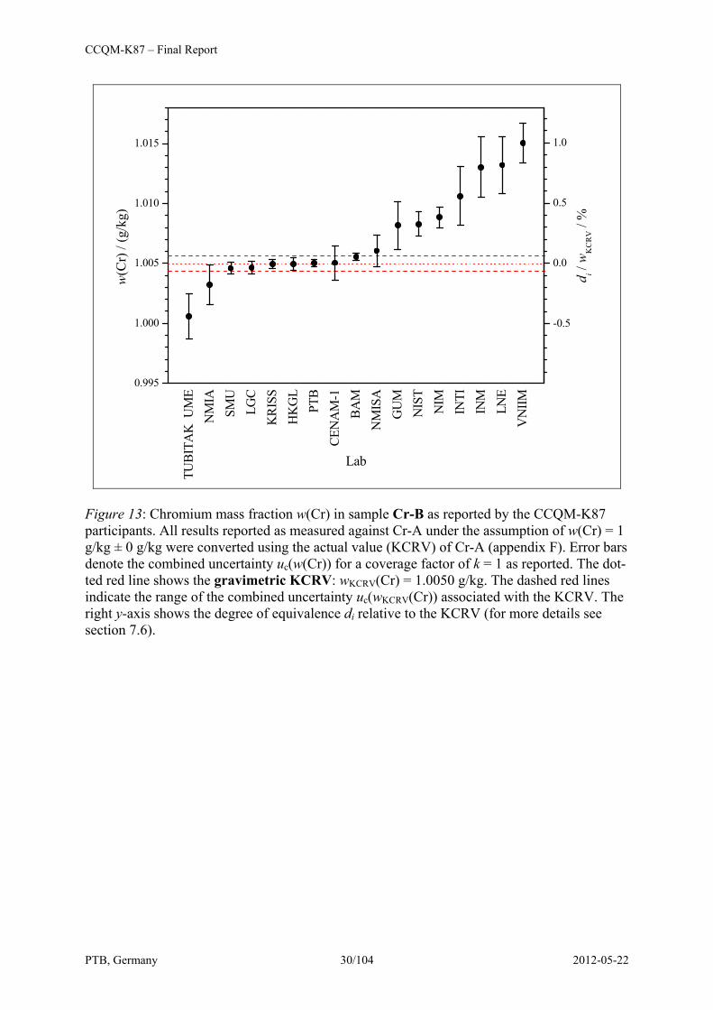
Figure 13: Chromium mass fraction w(Cr) in sample Cr-B as reported by the CCQM-K87 participants. All results reported as measured against Cr-A under the assumption of w(Cr) = 1 g/kg ± 0 g/kg were converted using the actual value (KCRV) of Cr-A (appendix F). Error bars denote the combined uncertainty uc(w(Cr)) for a coverage factor of k = 1 as reported. The dot-ted red line shows the gravimetric KCRV: wKCRV(Cr) = 1.0050 g/kg. The dashed red lines indicate the range of the combined uncertainty uc(wKCRV(Cr)) associated with the KCRV. The right y-axis shows the degree of equivalence di relative to the KCRV (for more details see section 7.6).
CCQM-K87 – Final Report
PTB, Germany 31/104 2012-05-22
TUBI
TAK
UM
E
CEN
AM
-1
SMU
KRI
SS
NM
IA
NM
ISA
INTI
PTB
BAM
NIS
T
NIM
GU
M
LNE
VN
IIM
0.975
0.980
0.985
0.990
0.995
1.000w
(Cr)
/ (g
/kg)
Lab
-1.0
-0.5
0.0
0.5
1.0
1.5
di /
wK
CR
V /
%
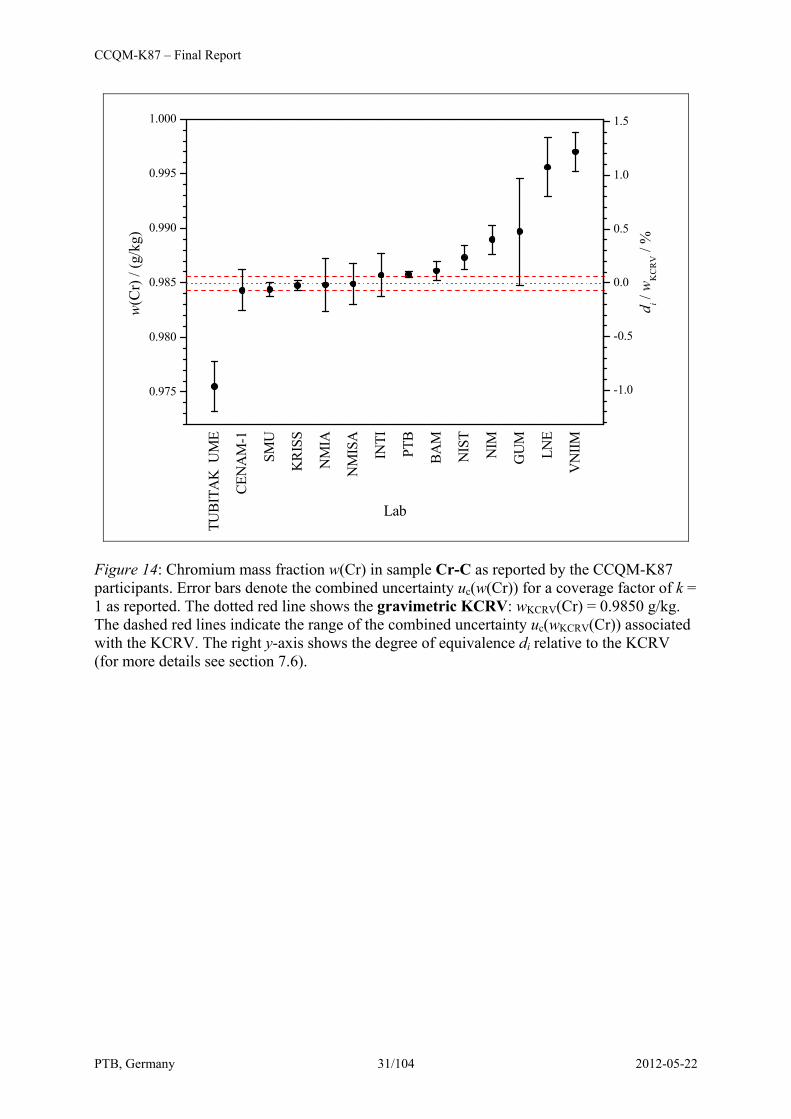
Figure 14: Chromium mass fraction w(Cr) in sample Cr-C as reported by the CCQM-K87 participants. Error bars denote the combined uncertainty uc(w(Cr)) for a coverage factor of k = 1 as reported. The dotted red line shows the gravimetric KCRV: wKCRV(Cr) = 0.9850 g/kg. The dashed red lines indicate the range of the combined uncertainty uc(wKCRV(Cr)) associated with the KCRV. The right y-axis shows the degree of equivalence di relative to the KCRV (for more details see section 7.6).
CCQM-K87 – Final Report
PTB, Germany 32/104 2012-05-22
7.4.2 Cobalt
NM
IA
NIM PT
B
CEN
AM
-1
NM
IJ
KRI
SS
NIS
T
NM
ISA
HK
GL
GU
M
TUBI
TAK
UM
E
INM
ETRO INTI
LGC
INM
VN
IIM
0.975
0.980
0.985
0.990
0.995
1.000
1.005
1.010
w(C
o) /
(g/k
g)
Lab
-0.5
0.0
0.5
1.0
1.5
2.0
2.5
3.0
di /
wK
CR
V /
%
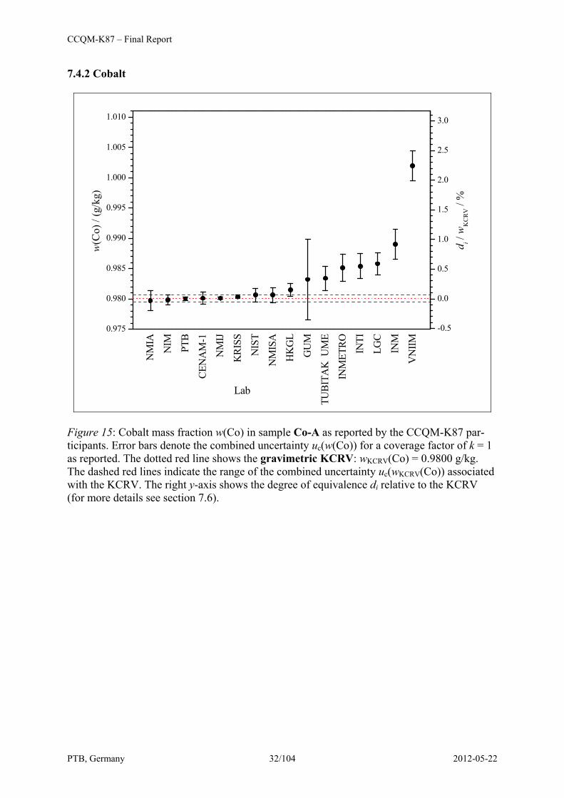
Figure 15: Cobalt mass fraction w(Co) in sample Co-A as reported by the CCQM-K87 par-ticipants. Error bars denote the combined uncertainty uc(w(Co)) for a coverage factor of k = 1 as reported. The dotted red line shows the gravimetric KCRV: wKCRV(Co) = 0.9800 g/kg. The dashed red lines indicate the range of the combined uncertainty uc(wKCRV(Co)) associated with the KCRV. The right y-axis shows the degree of equivalence di relative to the KCRV (for more details see section 7.6).
CCQM-K87 – Final Report
PTB, Germany 33/104 2012-05-22
INTI
VN
IIM INM
GU
MIN
MET
RO NIM
TUBI
TAK
UM
EN
MIS
AN
MIA
LNE
HK
GL
NM
IJK
RISS
CEN
AM
-1SM
UPT
BLG
CN
IST
0.985
0.990
0.995
1.000
1.005w
(Co)
/ (g
/kg)
Lab
-1.5
-1.0
-0.5
0.0
0.5
di /
wK
CR
V /
%
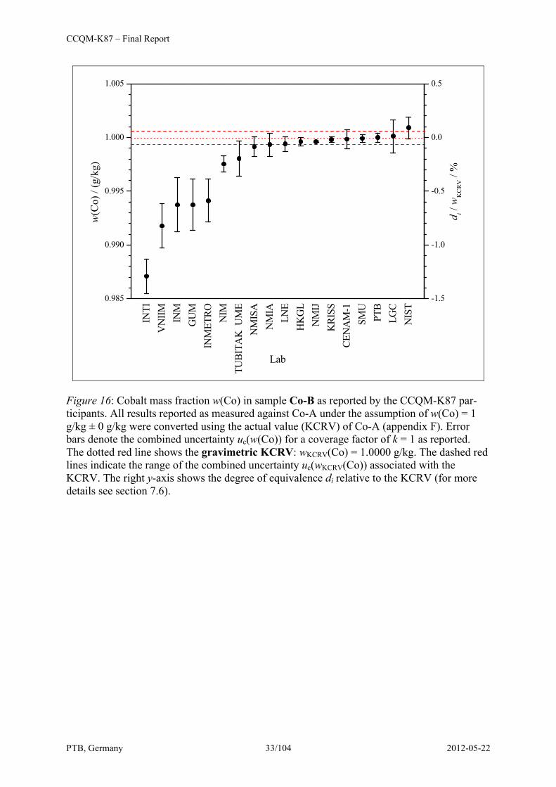
Figure 16: Cobalt mass fraction w(Co) in sample Co-B as reported by the CCQM-K87 par-ticipants. All results reported as measured against Co-A under the assumption of w(Co) = 1 g/kg ± 0 g/kg were converted using the actual value (KCRV) of Co-A (appendix F). Error bars denote the combined uncertainty uc(w(Co)) for a coverage factor of k = 1 as reported. The dotted red line shows the gravimetric KCRV: wKCRV(Co) = 1.0000 g/kg. The dashed red lines indicate the range of the combined uncertainty uc(wKCRV(Co)) associated with the KCRV. The right y-axis shows the degree of equivalence di relative to the KCRV (for more details see section 7.6).
CCQM-K87 – Final Report
PTB, Germany 34/104 2012-05-22
VN
IIM INTI
TUBI
TAK
UM
E
NIM
LNE
CEN
AM
-1
NM
ISA
KRI
SS
NM
IJ
PTB
SMU
GU
M
INM
ETRO
NIS
T
NM
IA
0.995
1.000
1.005
1.010
1.015
1.020
1.025w
(Co)
/ (g
/kg)
Lab
-2.0
-1.5
-1.0
-0.5
0.0
0.5
di /
wK
CR
V /
%
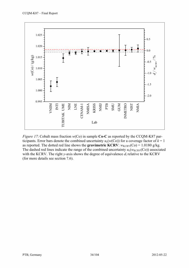
Figure 17: Cobalt mass fraction w(Co) in sample Co-C as reported by the CCQM-K87 par-ticipants. Error bars denote the combined uncertainty uc(w(Co)) for a coverage factor of k = 1 as reported. The dotted red line shows the gravimetric KCRV: wKCRV(Co) = 1.0180 g/kg. The dashed red lines indicate the range of the combined uncertainty uc(wKCRV(Co)) associated with the KCRV. The right y-axis shows the degree of equivalence di relative to the KCRV (for more details see section 7.6).
CCQM-K87 – Final Report
PTB, Germany 35/104 2012-05-22
7.4.3 Lead
BAM
NM
IJ
PTB
LGC
NIM
KRI
SS
CEN
AM
-1
HK
GL
NIS
T
NM
IA
NM
ISA
INM
TUBI
TAK
UM
E
VN
IIM INTI
GU
M
0.975
0.980
0.985
0.990
0.995
1.000
1.005
1.010
1.03
59
w(P
b) /
(g/k
g)
Lab
-0.5
0.0
0.5
1.0
1.5
2.0
2.5
3.0
di /
wK
CR
V /
%
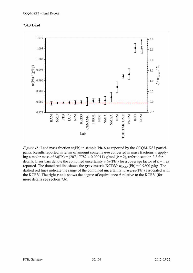
Figure 18: Lead mass fraction w(Pb) in sample Pb-A as reported by the CCQM-K87 partici-pants. Results reported in terms of amount contents n/m converted in mass fractions w apply-ing a molar mass of M(Pb) = (207.17782 ± 0.00011) g/mol (k = 2), refer to section 2.3 for details. Error bars denote the combined uncertainty uc(w(Pb)) for a coverage factor of k = 1 as reported. The dotted red line shows the gravimetric KCRV: wKCRV(Pb) = 0.9800 g/kg. The dashed red lines indicate the range of the combined uncertainty uc(wKCRV(Pb)) associated with the KCRV. The right y-axis shows the degree of equivalence di relative to the KCRV (for more details see section 7.6).

CCQM-K87 – Final Report
PTB, Germany 36/104 2012-05-22
INTI
TUBI
TAK
UM
EN
MIA
CEN
AM
-2N
IST
HK
GL
KRI
SSPT
BLG
CSM
UBA
MCE
NA
M-1
NM
IJIN
MN
IMG
UM
LNE
NM
ISA
VN
IIM
0.985
0.990
0.995
1.000
w(P
b) /
(g/k
g)
Lab
-1.0
-0.5
0.0
0.5
di /
wK
CR
V /
%
Figure 19: Lead mass fraction w(Pb) in sample Pb-B as reported by the CCQM-K87 partici-pants. All results reported as measured against Pb-A under the assumption of w(Pb) = 1 g/kg ± 0 g/kg were converted using the actual value (KCRV) of Pb-A (appendix F). Results re-ported in terms of amount contents n/m converted in mass fractions w applying a molar mass of M(Pb) = (207.17782 ± 0.00011) g/mol (k = 2), refer to section 2.3 for details. Error bars denote the combined uncertainty uc(w(Pb)) for a coverage factor of k = 1 as reported. The dotted red line shows the gravimetric KCRV: wKCRV(Pb) = 0.9940 g/kg. The dashed red lines indicate the range of the combined uncertainty uc(wKCRV(Pb)) associated with the KCRV. The right y-axis shows the degree of equivalence di relative to the KCRV (for more details see section 7.6).
CCQM-K87 – Final Report
PTB, Germany 37/104 2012-05-22
NM
ISA
NM
IA
BAM
NIM
KRI
SS
NM
IJ
PTB
SMU
CEN
AM
-1
NIS
T
CEN
AM
-2
LNE
TUBI
TAK
UM
E
INTI
VN
IIM
GU
M
0.975
0.980
0.985
0.990
0.995
1.000w
(Pb)
/ (g
/kg)
Lab
-0.5
0.0
0.5
1.0
1.5
1.03
80
di /
wK
CR
V /
%
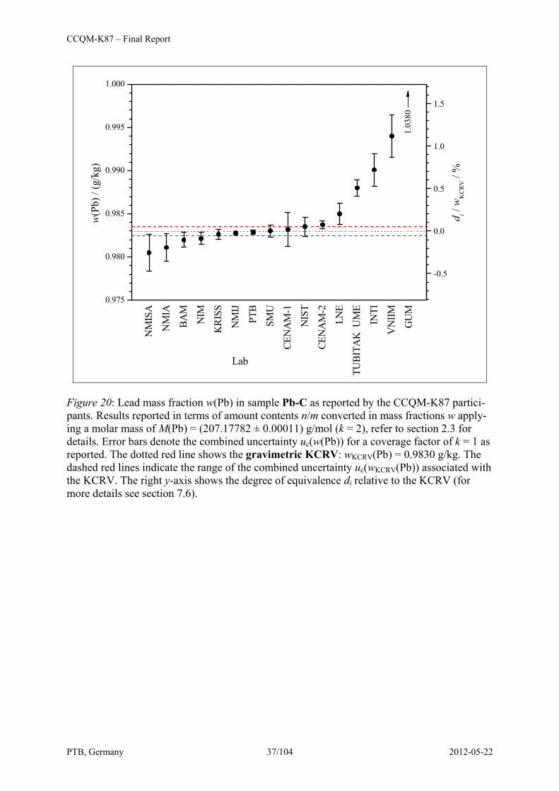
Figure 20: Lead mass fraction w(Pb) in sample Pb-C as reported by the CCQM-K87 partici-pants. Results reported in terms of amount contents n/m converted in mass fractions w apply-ing a molar mass of M(Pb) = (207.17782 ± 0.00011) g/mol (k = 2), refer to section 2.3 for details. Error bars denote the combined uncertainty uc(w(Pb)) for a coverage factor of k = 1 as reported. The dotted red line shows the gravimetric KCRV: wKCRV(Pb) = 0.9830 g/kg. The dashed red lines indicate the range of the combined uncertainty uc(wKCRV(Pb)) associated with the KCRV. The right y-axis shows the degree of equivalence di relative to the KCRV (for more details see section 7.6).
CCQM-K87 – Final Report
PTB, Germany 38/104 2012-05-22
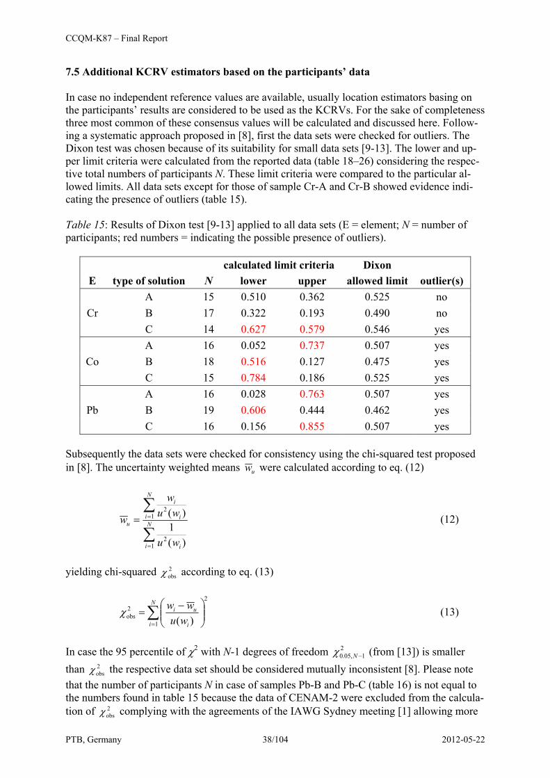
7.5 Additional KCRV estimators based on the participants’ data In case no independent reference values are available, usually location estimators basing on the participants’ results are considered to be used as the KCRVs. For the sake of completeness three most common of these consensus values will be calculated and discussed here. Follow-ing a systematic approach proposed in [8], first the data sets were checked for outliers. The Dixon test was chosen because of its suitability for small data sets [9-13]. The lower and up-per limit criteria were calculated from the reported data (table 18–26) considering the respec-tive total numbers of participants N. These limit criteria were compared to the particular al-lowed limits. All data sets except for those of sample Cr-A and Cr-B showed evidence indi-cating the presence of outliers (table 15). Table 15: Results of Dixon test [9-13] applied to all data sets (E = element; N = number of participants; red numbers = indicating the possible presence of outliers).
calculated limit criteria Dixon
E type of solution N lower upper allowed limit outlier(s)
Cr A 15 0.510 0.362 0.525 no B 17 0.322 0.193 0.490 no C 14 0.627 0.579 0.546 yes
Co A 16 0.052 0.737 0.507 yes B 18 0.516 0.127 0.475 yes C 15 0.784 0.186 0.525 yes
Pb A 16 0.028 0.763 0.507 yes B 19 0.606 0.444 0.462 yes C 16 0.156 0.855 0.507 yes
Subsequently the data sets were checked for consistency using the chi-squared test proposed in [8]. The uncertainty weighted means uw were calculated according to eq. (12)
∑
∑
=
== N
i i
N
i i
i
u
wu
wuw
w
12
12
)(1
)( (12)
yielding chi-squared 2
obsχ according to eq. (13)
∑=
⎟⎟⎠
⎞⎜⎜⎝
⎛ −=
N
i i
ui
wuww
1
22obs )(
χ (13)
In case the 95 percentile of χ2 with N-1 degrees of freedom 2
1,05.0 −Nχ (from [13]) is smaller than 2
obsχ the respective data set should be considered mutually inconsistent [8]. Please note that the number of participants N in case of samples Pb-B and Pb-C (table 16) is not equal to the numbers found in table 15 because the data of CENAM-2 were excluded from the calcula-tion of 2
obsχ complying with the agreements of the IAWG Sydney meeting [1] allowing more

CCQM-K87 – Final Report
PTB, Germany 39/104 2012-05-22
than one result to be reported in a key comparison but allowing only one of these to be in-cluded in a (potential) KCRV estimator. All nine data sets did not pass the chi-squared test (table 16). This finding renders any KCRV estimator based on the participants’ results ques-tionable considering the availability of a gravimetric reference value. Table 16: Results of chi-squared test [8] applied to all data sets (E = element, N = number of participants). Values rounded to yield integer numbers.
E type of solution N 2obsχ 2
1,05.0 −Nχ mutually consistent?
Cr A 15 113 24 no B 17 103 26 no C 14 92 22 no
Co A 16 113 25 no B 18 107 28 no C 15 95 24 no
Pb A 16 404 25 no B 18 90 28 no C 15 116 24 no
Nevertheless the uncertainty weighted mean uw (eq. (12)) as well as the arithmetic mean w (eq. (14)) and the median mw (eq. (15)) were calculated along with their associated uncertain-ties )( uwu , )(wu and )( mwu (equations 17–19).
∑=
=N
iiw
Nw
1
1 (14)
( ) even21
12/2/ Nwww NNm ++= (15)
odd2/)1( Nww Nm += (16) Due to the observed mutual inconsistency of all data sets the uncertainty )( uwu associated with the uncertainty weighted mean was corrected for the observed dispersion according to [8].
1
12
2obs
)(1
1)(
−
=⎟⎟⎠
⎞⎜⎜⎝
⎛= ∑
N
i iu wuN-
wu χ (17)
( ) ( )∑=
−⋅
=N
ii ww
N-Nwu
1
2
11)( (18)
( )mim wwN
wu −⋅⋅= med483.12
)( π (19)
CCQM-K87 – Final Report
PTB, Germany 40/104 2012-05-22
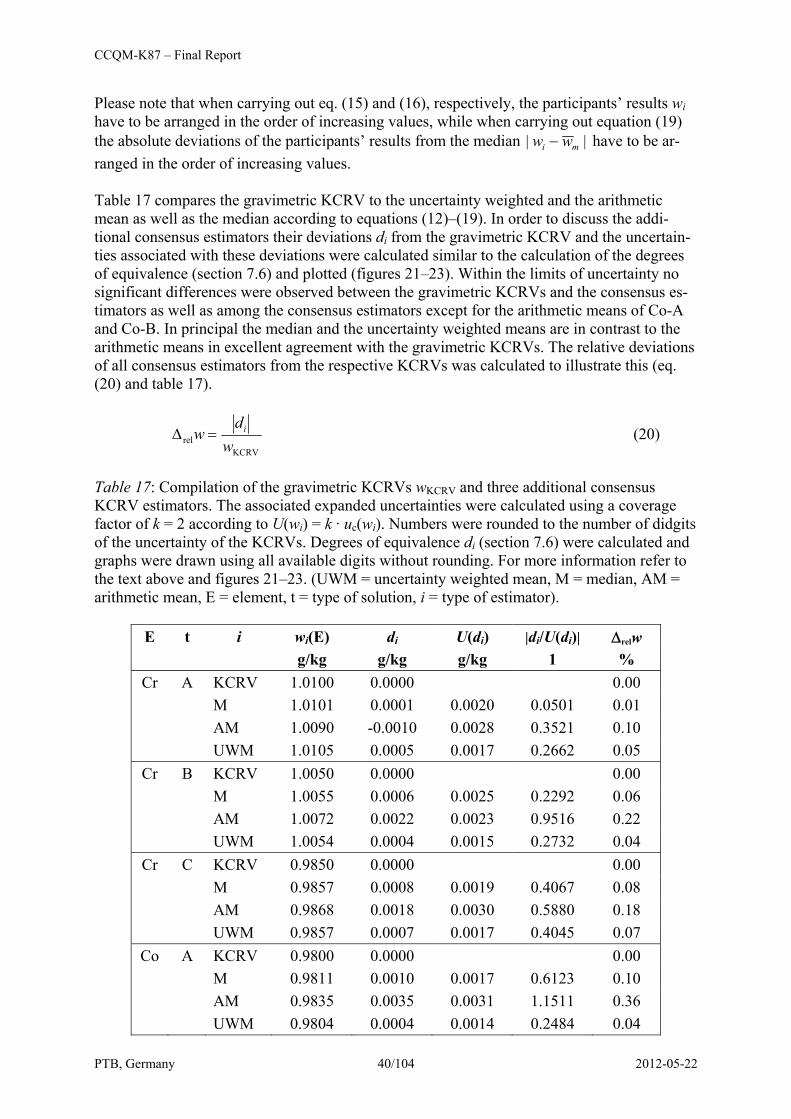
Please note that when carrying out eq. (15) and (16), respectively, the participants’ results wi have to be arranged in the order of increasing values, while when carrying out equation (19) the absolute deviations of the participants’ results from the median || mi ww − have to be ar-ranged in the order of increasing values. Table 17 compares the gravimetric KCRV to the uncertainty weighted and the arithmetic mean as well as the median according to equations (12)–(19). In order to discuss the addi-tional consensus estimators their deviations di from the gravimetric KCRV and the uncertain-ties associated with these deviations were calculated similar to the calculation of the degrees of equivalence (section 7.6) and plotted (figures 21–23). Within the limits of uncertainty no significant differences were observed between the gravimetric KCRVs and the consensus es-timators as well as among the consensus estimators except for the arithmetic means of Co-A and Co-B. In principal the median and the uncertainty weighted means are in contrast to the arithmetic means in excellent agreement with the gravimetric KCRVs. The relative deviations of all consensus estimators from the respective KCRVs was calculated to illustrate this (eq. (20) and table 17).
KCRV
rel wd
w i=Δ (20)
Table 17: Compilation of the gravimetric KCRVs wKCRV and three additional consensus KCRV estimators. The associated expanded uncertainties were calculated using a coverage factor of k = 2 according to U(wi) = k · uc(wi). Numbers were rounded to the number of didgits of the uncertainty of the KCRVs. Degrees of equivalence di (section 7.6) were calculated and graphs were drawn using all available digits without rounding. For more information refer to the text above and figures 21–23. (UWM = uncertainty weighted mean, M = median, AM = arithmetic mean, E = element, t = type of solution, i = type of estimator).
E t i wi(E) di U(di) |di/U(di)| Δrelw g/kg g/kg g/kg 1 %
Cr A KCRV 1.0100 0.0000 0.00 M 1.0101 0.0001 0.0020 0.0501 0.01 AM 1.0090 -0.0010 0.0028 0.3521 0.10 UWM 1.0105 0.0005 0.0017 0.2662 0.05
Cr B KCRV 1.0050 0.0000 0.00 M 1.0055 0.0006 0.0025 0.2292 0.06 AM 1.0072 0.0022 0.0023 0.9516 0.22 UWM 1.0054 0.0004 0.0015 0.2732 0.04
Cr C KCRV 0.9850 0.0000 0.00 M 0.9857 0.0008 0.0019 0.4067 0.08 AM 0.9868 0.0018 0.0030 0.5880 0.18 UWM 0.9857 0.0007 0.0017 0.4045 0.07
Co A KCRV 0.9800 0.0000 0.00 M 0.9811 0.0010 0.0017 0.6123 0.10 AM 0.9835 0.0035 0.0031 1.1511 0.36 UWM 0.9804 0.0004 0.0014 0.2484 0.04
CCQM-K87 – Final Report
PTB, Germany 41/104 2012-05-22
E t i wi(E) di U(di) |di/U(di)| Δrelw g/kg g/kg g/kg 1 %
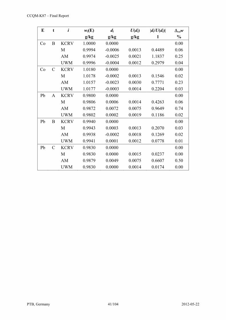
Co B KCRV 1.0000 0.0000 0.00 M 0.9994 -0.0006 0.0013 0.4489 0.06 AM 0.9974 -0.0025 0.0021 1.1837 0.25 UWM 0.9996 -0.0004 0.0012 0.2979 0.04
Co C KCRV 1.0180 0.0000 0.00 M 1.0178 -0.0002 0.0013 0.1546 0.02 AM 1.0157 -0.0023 0.0030 0.7771 0.23 UWM 1.0177 -0.0003 0.0014 0.2204 0.03
Pb A KCRV 0.9800 0.0000 0.00 M 0.9806 0.0006 0.0014 0.4263 0.06 AM 0.9872 0.0072 0.0075 0.9649 0.74 UWM 0.9802 0.0002 0.0019 0.1186 0.02
Pb B KCRV 0.9940 0.0000 0.00 M 0.9943 0.0003 0.0013 0.2070 0.03 AM 0.9938 -0.0002 0.0018 0.1269 0.02 UWM 0.9941 0.0001 0.0012 0.0778 0.01
Pb C KCRV 0.9830 0.0000 0.00 M 0.9830 0.0000 0.0015 0.0237 0.00 AM 0.9879 0.0049 0.0075 0.6607 0.50 UWM 0.9830 0.0000 0.0014 0.0174 0.00

CCQM-K87 – Final Report
PTB, Germany 42/104 2012-05-22
med
ian
arith
met
ic m
ean
wei
ghte
d m
ean
med
ian
arith
met
ic m
ean
wei
ghte
d m
ean
med
ian
arith
met
ic m
ean
wei
ghte
d m
ean
-0.005
0.000
0.005
Cr-CCr-B
d i / (g
/kg)
Cr-A
Figure 21: Chromium samples. Deviation di of the medians, arithmetic means, and uncer-tainty weighted means from the gravimetric KCRVs along with the expanded uncertainties associated with these deviations; di calculated similar to degrees of equivalence (section 7.6). The dashed red line indicates the relative location of the gravimetric KCRVs. Within the lim-its of uncertainty no significant differences between the estimators were observed. Medians and uncertainty weighted means are in excellent agreement with the KCRVs.
CCQM-K87 – Final Report
PTB, Germany 43/104 2012-05-22
med
ian
arith
met
ic m
ean
wei
ghte
d m
ean
med
ian
arith
met
ic m
ean
wei
ghte
d m
ean
med
ian
arith
met
ic m
ean
wei
ghte
d m
ean
-0.005
0.000
0.005
d i / (g
/kg)
Co-A Co-B Co-C
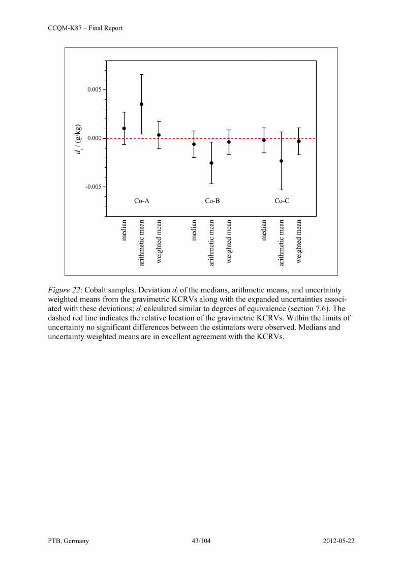
Figure 22: Cobalt samples. Deviation di of the medians, arithmetic means, and uncertainty weighted means from the gravimetric KCRVs along with the expanded uncertainties associ-ated with these deviations; di calculated similar to degrees of equivalence (section 7.6). The dashed red line indicates the relative location of the gravimetric KCRVs. Within the limits of uncertainty no significant differences between the estimators were observed. Medians and uncertainty weighted means are in excellent agreement with the KCRVs.
CCQM-K87 – Final Report
PTB, Germany 44/104 2012-05-22
med
ian
arith
met
ic m
ean
wei
ghte
d m
ean
med
ian
arith
met
ic m
ean
wei
ghte
d m
ean
med
ian
arith
met
ic m
ean
wei
ghte
d m
ean
-0.005
0.000
0.005
d i / (g
/kg)
Pb-A Pb-B Pb-C
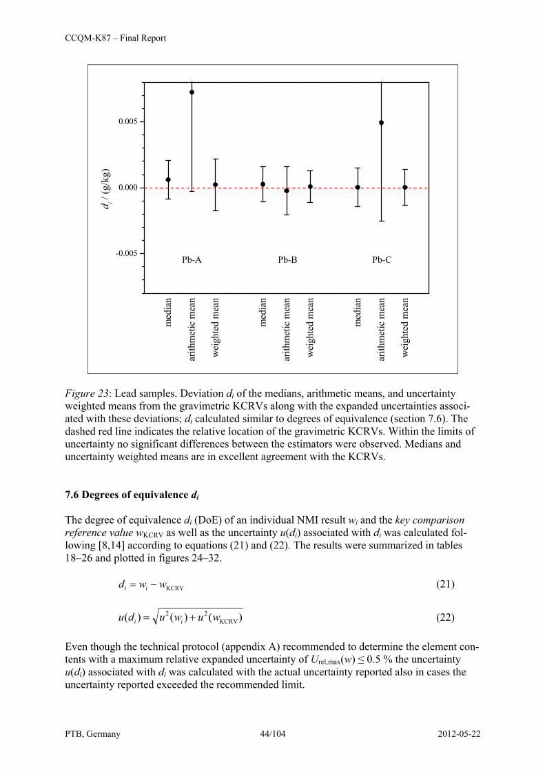
Figure 23: Lead samples. Deviation di of the medians, arithmetic means, and uncertainty weighted means from the gravimetric KCRVs along with the expanded uncertainties associ-ated with these deviations; di calculated similar to degrees of equivalence (section 7.6). The dashed red line indicates the relative location of the gravimetric KCRVs. Within the limits of uncertainty no significant differences between the estimators were observed. Medians and uncertainty weighted means are in excellent agreement with the KCRVs. 7.6 Degrees of equivalence di The degree of equivalence di (DoE) of an individual NMI result wi and the key comparison reference value wKCRV as well as the uncertainty u(di) associated with di was calculated fol-lowing [8,14] according to equations (21) and (22). The results were summarized in tables 18–26 and plotted in figures 24–32. KCRVwwd ii −= (21) )()()( KCRV
22 wuwudu ii += (22) Even though the technical protocol (appendix A) recommended to determine the element con-tents with a maximum relative expanded uncertainty of Urel,max(w) ≤ 0.5 % the uncertainty u(di) associated with di was calculated with the actual uncertainty reported also in cases the uncertainty reported exceeded the recommended limit.

CCQM-K87 – Final Report
PTB, Germany 45/104 2012-05-22
Table 18: Chromium sample Cr-A. Mass fractions wi(Cr) and their associated combined and relative expanded uncertainties uc(wi) and Urel(wi), resp., together with the coverage factor ki as reported by the participants in the order of increasing mass fraction values. In case only expanded or relative combined uncertainties were reported the values compiled were calcu-lated accordingly. Degrees of equivalence di and their associated combined and expanded uncertainty u(di) and U(di), resp., according to equation (21) and (22). A coverage factor of k = 2 was used to calculate U(di) = k · u(di).
Cr-A
wKCRV(Cr) = (1.0100 ± 0.0013) g/kg
NMI wi(Cr) uc(wi) ki Urel(wi) di u(di) U(di)
g/kg g/kg 1 % g/kg g/kg g/kg VNIIM 0.997 0.00209 2 0.42 -0.01300 0.0022 0.0044 TUBITAK UME 1.0028 0.00236 2 0.47 -0.00720 0.0024 0.0049 INTI 1.0047 0.00250 2 0.50 -0.00530 0.0026 0.0052 CENAM-1 1.0063 0.00203 2 0.40 -0.00374 0.0021 0.0043 HKGL 1.0085 0.00129 2.11 0.27 -0.00150 0.0014 0.0029 NMISA 1.0096 0.00206 1.99 0.41 -0.00040 0.0022 0.0043 KRISS 1.00991 0.00031 2.57 0.08 -0.00009 0.0007 0.0014 NMIA 1.0101 0.00157 2.10 0.33 0.00010 0.0017 0.0034 LGC 1.0104 0.00180 2 0.36 0.00040 0.0019 0.0038 PTB 1.01068 0.00033 2 0.06 0.00068 0.0007 0.0015 BAM 1.0109 0.00090 2 0.18 0.00090 0.0011 0.0022 INM 1.0110 0.00255 2 0.50 0.00100 0.0026 0.0053 NIST 1.0121 0.00110 2.045 0.22 0.00210 0.0013 0.0026 NIM 1.0150 0.00070 2 0.14 0.00495 0.0010 0.0019 GUM 1.0163 0.00500 2 0.98 0.00630 0.0050 0.0101
CCQM-K87 – Final Report
PTB, Germany 46/104 2012-05-22
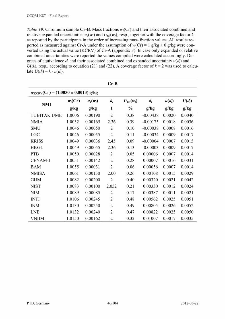
Table 19: Chromium sample Cr-B. Mass fractions wi(Cr) and their associated combined and relative expanded uncertainties uc(wi) and Urel(wi), resp., together with the coverage factor ki as reported by the participants in the order of increasing mass fraction values. All results re-ported as measured against Cr-A under the assumption of w(Cr) = 1 g/kg ± 0 g/kg were con-verted using the actual value (KCRV) of Cr-A (appendix F). In case only expanded or relative combined uncertainties were reported the values compiled were calculated accordingly. De-grees of equivalence di and their associated combined and expanded uncertainty u(di) and U(di), resp., according to equation (21) and (22). A coverage factor of k = 2 was used to calcu-late U(di) = k · u(di).
Cr-B
wKCRV(Cr) = (1.0050 ± 0.0013) g/kg
NMI wi(Cr) uc(wi) ki Urel(wi) di u(di) U(di)
g/kg g/kg 1 % g/kg g/kg g/kg TUBITAK UME 1.0006 0.00190 2 0.38 -0.00438 0.0020 0.0040 NMIA 1.0032 0.00165 2.36 0.39 -0.00175 0.0018 0.0036 SMU 1.0046 0.00050 2 0.10 -0.00038 0.0008 0.0016 LGC 1.0046 0.00055 2 0.11 -0.00034 0.0009 0.0017 KRISS 1.0049 0.00036 2.45 0.09 -0.00004 0.0007 0.0015 HKGL 1.0049 0.00055 2.36 0.13 -0.00003 0.0009 0.0017 PTB 1.0050 0.00028 2 0.05 0.00006 0.0007 0.0014 CENAM-1 1.0051 0.00142 2 0.28 0.00007 0.0016 0.0031 BAM 1.0055 0.00031 2 0.06 0.00056 0.0007 0.0014 NMISA 1.0061 0.00130 2.00 0.26 0.00108 0.0015 0.0029 GUM 1.0082 0.00200 2 0.40 0.00320 0.0021 0.0042 NIST 1.0083 0.00100 2.052 0.21 0.00330 0.0012 0.0024 NIM 1.0089 0.00085 2 0.17 0.00387 0.0011 0.0021 INTI 1.0106 0.00245 2 0.48 0.00562 0.0025 0.0051 INM 1.0130 0.00250 2 0.49 0.00805 0.0026 0.0052 LNE 1.0132 0.00240 2 0.47 0.00822 0.0025 0.0050 VNIIM 1.0150 0.00162 2 0.32 0.01007 0.0017 0.0035

CCQM-K87 – Final Report
PTB, Germany 47/104 2012-05-22
Table 20: Chromium sample Cr-C. Mass fractions wi(Cr) and their associated combined and relative expanded uncertainties uc(wi) and Urel(wi), resp., together with the coverage factor ki as reported by the participants in the order of increasing mass fraction values. In case only expanded or relative combined uncertainties were reported the values compiled were calcu-lated accordingly. Degrees of equivalence di and their associated combined and expanded uncertainty u(di) and U(di), resp., according to equation (21) and (22). A coverage factor of k = 2 was used to calculate U(di) = k · u(di).
Cr-C
wKCRV(Cr) = (0.9850 ± 0.0013) g/kg
NMI wi(Cr) uc(wi) ki Urel(wi) di u(di) U(di)
g/kg g/kg 1 % g/kg g/kg g/kg TUBITAK UME 0.9755 0.00229 2 0.47 -0.00948 0.0024 0.0048 CENAM-1 0.9843 0.00184 2 0.37 -0.00064 0.0019 0.0039 SMU 0.9844 0.00065 2 0.13 -0.00058 0.0009 0.0018 KRISS 0.98476 0.00044 2.78 0.12 -0.00022 0.0008 0.0016 NMIA 0.9848 0.00244 2.01 0.50 -0.00018 0.0025 0.0050 NMISA 0.9849 0.00191 1.99 0.39 -0.00008 0.0020 0.0040 INTI 0.9857 0.00195 2 0.40 0.00072 0.0021 0.0041 PTB 0.98578 0.00030 2 0.06 0.00080 0.0007 0.0014 BAM 0.9861 0.00085 2 0.17 0.00112 0.0011 0.0021 NIST 0.9873 0.00110 2.042 0.22 0.00232 0.0013 0.0025 NIM 0.9889 0.00130 2 0.26 0.00397 0.0014 0.0029 GUM 0.9897 0.00490 2 0.99 0.00472 0.0049 0.0099 LNE 0.9956 0.00270 2 0.54 0.01062 0.0028 0.0055 VNIIM 0.997 0.00179 2 0.36 0.01202 0.0019 0.0038
CCQM-K87 – Final Report
PTB, Germany 48/104 2012-05-22
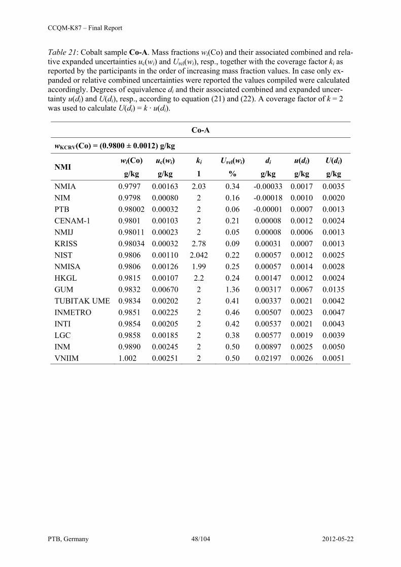
Table 21: Cobalt sample Co-A. Mass fractions wi(Co) and their associated combined and rela-tive expanded uncertainties uc(wi) and Urel(wi), resp., together with the coverage factor ki as reported by the participants in the order of increasing mass fraction values. In case only ex-panded or relative combined uncertainties were reported the values compiled were calculated accordingly. Degrees of equivalence di and their associated combined and expanded uncer-tainty u(di) and U(di), resp., according to equation (21) and (22). A coverage factor of k = 2 was used to calculate U(di) = k · u(di).
Co-A
wKCRV(Co) = (0.9800 ± 0.0012) g/kg
NMI wi(Co) uc(wi) ki Urel(wi) di u(di) U(di)
g/kg g/kg 1 % g/kg g/kg g/kg NMIA 0.9797 0.00163 2.03 0.34 -0.00033 0.0017 0.0035 NIM 0.9798 0.00080 2 0.16 -0.00018 0.0010 0.0020 PTB 0.98002 0.00032 2 0.06 -0.00001 0.0007 0.0013 CENAM-1 0.9801 0.00103 2 0.21 0.00008 0.0012 0.0024 NMIJ 0.98011 0.00023 2 0.05 0.00008 0.0006 0.0013 KRISS 0.98034 0.00032 2.78 0.09 0.00031 0.0007 0.0013 NIST 0.9806 0.00110 2.042 0.22 0.00057 0.0012 0.0025 NMISA 0.9806 0.00126 1.99 0.25 0.00057 0.0014 0.0028 HKGL 0.9815 0.00107 2.2 0.24 0.00147 0.0012 0.0024 GUM 0.9832 0.00670 2 1.36 0.00317 0.0067 0.0135 TUBITAK UME 0.9834 0.00202 2 0.41 0.00337 0.0021 0.0042 INMETRO 0.9851 0.00225 2 0.46 0.00507 0.0023 0.0047 INTI 0.9854 0.00205 2 0.42 0.00537 0.0021 0.0043 LGC 0.9858 0.00185 2 0.38 0.00577 0.0019 0.0039 INM 0.9890 0.00245 2 0.50 0.00897 0.0025 0.0050 VNIIM 1.002 0.00251 2 0.50 0.02197 0.0026 0.0051
CCQM-K87 – Final Report
PTB, Germany 49/104 2012-05-22
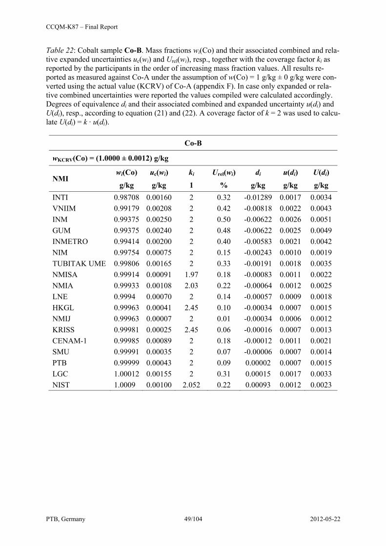
Table 22: Cobalt sample Co-B. Mass fractions wi(Co) and their associated combined and rela-tive expanded uncertainties uc(wi) and Urel(wi), resp., together with the coverage factor ki as reported by the participants in the order of increasing mass fraction values. All results re-ported as measured against Co-A under the assumption of w(Co) = 1 g/kg ± 0 g/kg were con-verted using the actual value (KCRV) of Co-A (appendix F). In case only expanded or rela-tive combined uncertainties were reported the values compiled were calculated accordingly. Degrees of equivalence di and their associated combined and expanded uncertainty u(di) and U(di), resp., according to equation (21) and (22). A coverage factor of k = 2 was used to calcu-late U(di) = k · u(di).
Co-B
wKCRV(Co) = (1.0000 ± 0.0012) g/kg
NMI wi(Co) uc(wi) ki Urel(wi) di u(di) U(di)
g/kg g/kg 1 % g/kg g/kg g/kg INTI 0.98708 0.00160 2 0.32 -0.01289 0.0017 0.0034 VNIIM 0.99179 0.00208 2 0.42 -0.00818 0.0022 0.0043 INM 0.99375 0.00250 2 0.50 -0.00622 0.0026 0.0051 GUM 0.99375 0.00240 2 0.48 -0.00622 0.0025 0.0049 INMETRO 0.99414 0.00200 2 0.40 -0.00583 0.0021 0.0042 NIM 0.99754 0.00075 2 0.15 -0.00243 0.0010 0.0019 TUBITAK UME 0.99806 0.00165 2 0.33 -0.00191 0.0018 0.0035 NMISA 0.99914 0.00091 1.97 0.18 -0.00083 0.0011 0.0022 NMIA 0.99933 0.00108 2.03 0.22 -0.00064 0.0012 0.0025 LNE 0.9994 0.00070 2 0.14 -0.00057 0.0009 0.0018 HKGL 0.99963 0.00041 2.45 0.10 -0.00034 0.0007 0.0015 NMIJ 0.99963 0.00007 2 0.01 -0.00034 0.0006 0.0012 KRISS 0.99981 0.00025 2.45 0.06 -0.00016 0.0007 0.0013 CENAM-1 0.99985 0.00089 2 0.18 -0.00012 0.0011 0.0021 SMU 0.99991 0.00035 2 0.07 -0.00006 0.0007 0.0014 PTB 0.99999 0.00043 2 0.09 0.00002 0.0007 0.0015 LGC 1.00012 0.00155 2 0.31 0.00015 0.0017 0.0033 NIST 1.0009 0.00100 2.052 0.22 0.00093 0.0012 0.0023
CCQM-K87 – Final Report
PTB, Germany 50/104 2012-05-22
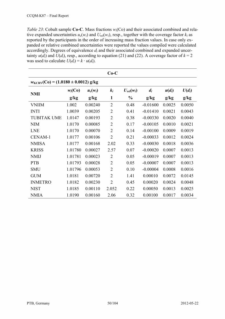
Table 23: Cobalt sample Co-C. Mass fractions wi(Co) and their associated combined and rela-tive expanded uncertainties uc(wi) and Urel(wi), resp., together with the coverage factor ki as reported by the participants in the order of increasing mass fraction values. In case only ex-panded or relative combined uncertainties were reported the values compiled were calculated accordingly. Degrees of equivalence di and their associated combined and expanded uncer-tainty u(di) and U(di), resp., according to equation (21) and (22). A coverage factor of k = 2 was used to calculate U(di) = k · u(di).
Co-C
wKCRV(Co) = (1.0180 ± 0.0012) g/kg
NMI wi(Co) uc(wi) ki Urel(wi) di u(di) U(di)
g/kg g/kg 1 % g/kg g/kg g/kg VNIIM 1.002 0.00240 2 0.48 -0.01600 0.0025 0.0050 INTI 1.0039 0.00205 2 0.41 -0.01410 0.0021 0.0043 TUBITAK UME 1.0147 0.00193 2 0.38 -0.00330 0.0020 0.0040 NIM 1.0170 0.00085 2 0.17 -0.00105 0.0010 0.0021 LNE 1.0170 0.00070 2 0.14 -0.00100 0.0009 0.0019 CENAM-1 1.0177 0.00106 2 0.21 -0.00033 0.0012 0.0024 NMISA 1.0177 0.00168 2.02 0.33 -0.00030 0.0018 0.0036 KRISS 1.01780 0.00027 2.57 0.07 -0.00020 0.0007 0.0013 NMIJ 1.01781 0.00023 2 0.05 -0.00019 0.0007 0.0013 PTB 1.01793 0.00028 2 0.05 -0.00007 0.0007 0.0013 SMU 1.01796 0.00053 2 0.10 -0.00004 0.0008 0.0016 GUM 1.0181 0.00720 2 1.41 0.00010 0.0072 0.0145 INMETRO 1.0182 0.00230 2 0.45 0.00020 0.0024 0.0048 NIST 1.0185 0.00110 2.052 0.22 0.00050 0.0013 0.0025 NMIA 1.0190 0.00160 2.06 0.32 0.00100 0.0017 0.0034
CCQM-K87 – Final Report
PTB, Germany 51/104 2012-05-22
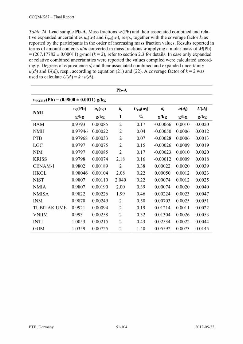
Table 24: Lead sample Pb-A. Mass fractions wi(Pb) and their associated combined and rela-tive expanded uncertainties uc(wi) and Urel(wi), resp., together with the coverage factor ki as reported by the participants in the order of increasing mass fraction values. Results reported in terms of amount contents n/m converted in mass fractions w applying a molar mass of M(Pb) = (207.17782 ± 0.00011) g/mol (k = 2), refer to section 2.3 for details. In case only expanded or relative combined uncertainties were reported the values compiled were calculated accord-ingly. Degrees of equivalence di and their associated combined and expanded uncertainty u(di) and U(di), resp., according to equation (21) and (22). A coverage factor of k = 2 was used to calculate U(di) = k · u(di).
Pb-A
wKCRV(Pb) = (0.9800 ± 0.0011) g/kg
NMI wi(Pb) uc(wi) ki Urel(wi) di u(di) U(di)
g/kg g/kg 1 % g/kg g/kg g/kg BAM 0.9793 0.00085 2 0.17 -0.00066 0.0010 0.0020 NMIJ 0.97946 0.00022 2 0.04 -0.00050 0.0006 0.0012 PTB 0.97968 0.00033 2 0.07 -0.00028 0.0006 0.0013 LGC 0.9797 0.00075 2 0.15 -0.00026 0.0009 0.0019 NIM 0.9797 0.00085 2 0.17 -0.00023 0.0010 0.0020 KRISS 0.9798 0.00074 2.18 0.16 -0.00012 0.0009 0.0018 CENAM-1 0.9802 0.00189 2 0.38 0.00022 0.0020 0.0039 HKGL 0.98046 0.00104 2.08 0.22 0.00050 0.0012 0.0023 NIST 0.9807 0.00110 2.040 0.22 0.00074 0.0012 0.0025 NMIA 0.9807 0.00190 2.00 0.39 0.00074 0.0020 0.0040 NMISA 0.9822 0.00226 1.99 0.46 0.00224 0.0023 0.0047 INM 0.9870 0.00249 2 0.50 0.00703 0.0025 0.0051 TUBITAK UME 0.9921 0.00094 2 0.19 0.01214 0.0011 0.0022 VNIIM 0.993 0.00258 2 0.52 0.01304 0.0026 0.0053 INTI 1.0053 0.00215 2 0.43 0.02534 0.0022 0.0044 GUM 1.0359 0.00725 2 1.40 0.05592 0.0073 0.0145
CCQM-K87 – Final Report
PTB, Germany 52/104 2012-05-22
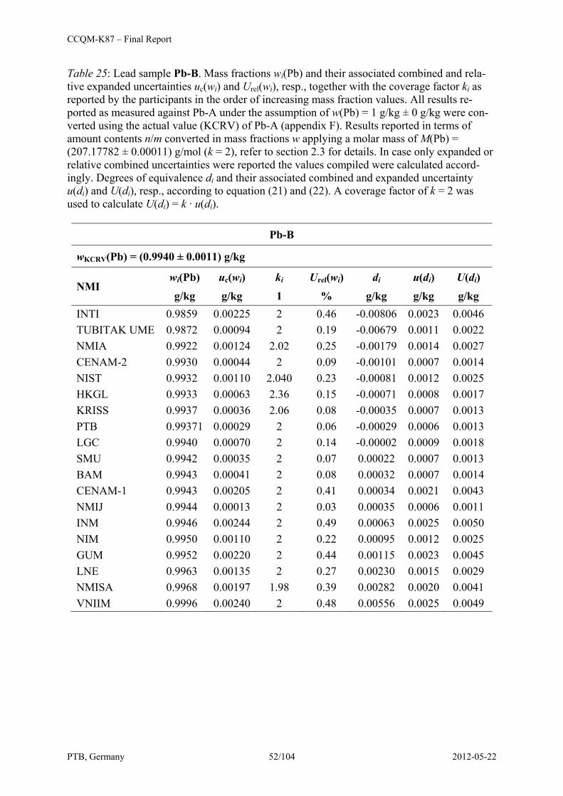
Table 25: Lead sample Pb-B. Mass fractions wi(Pb) and their associated combined and rela-tive expanded uncertainties uc(wi) and Urel(wi), resp., together with the coverage factor ki as reported by the participants in the order of increasing mass fraction values. All results re-ported as measured against Pb-A under the assumption of w(Pb) = 1 g/kg ± 0 g/kg were con-verted using the actual value (KCRV) of Pb-A (appendix F). Results reported in terms of amount contents n/m converted in mass fractions w applying a molar mass of M(Pb) = (207.17782 ± 0.00011) g/mol (k = 2), refer to section 2.3 for details. In case only expanded or relative combined uncertainties were reported the values compiled were calculated accord-ingly. Degrees of equivalence di and their associated combined and expanded uncertainty u(di) and U(di), resp., according to equation (21) and (22). A coverage factor of k = 2 was used to calculate U(di) = k · u(di).
Pb-B
wKCRV(Pb) = (0.9940 ± 0.0011) g/kg
NMI wi(Pb) uc(wi) ki Urel(wi) di u(di) U(di)
g/kg g/kg 1 % g/kg g/kg g/kg INTI 0.9859 0.00225 2 0.46 -0.00806 0.0023 0.0046 TUBITAK UME 0.9872 0.00094 2 0.19 -0.00679 0.0011 0.0022 NMIA 0.9922 0.00124 2.02 0.25 -0.00179 0.0014 0.0027 CENAM-2 0.9930 0.00044 2 0.09 -0.00101 0.0007 0.0014 NIST 0.9932 0.00110 2.040 0.23 -0.00081 0.0012 0.0025 HKGL 0.9933 0.00063 2.36 0.15 -0.00071 0.0008 0.0017 KRISS 0.9937 0.00036 2.06 0.08 -0.00035 0.0007 0.0013 PTB 0.99371 0.00029 2 0.06 -0.00029 0.0006 0.0013 LGC 0.9940 0.00070 2 0.14 -0.00002 0.0009 0.0018 SMU 0.9942 0.00035 2 0.07 0.00022 0.0007 0.0013 BAM 0.9943 0.00041 2 0.08 0.00032 0.0007 0.0014 CENAM-1 0.9943 0.00205 2 0.41 0.00034 0.0021 0.0043 NMIJ 0.9944 0.00013 2 0.03 0.00035 0.0006 0.0011 INM 0.9946 0.00244 2 0.49 0.00063 0.0025 0.0050 NIM 0.9950 0.00110 2 0.22 0.00095 0.0012 0.0025 GUM 0.9952 0.00220 2 0.44 0.00115 0.0023 0.0045 LNE 0.9963 0.00135 2 0.27 0.00230 0.0015 0.0029 NMISA 0.9968 0.00197 1.98 0.39 0.00282 0.0020 0.0041 VNIIM 0.9996 0.00240 2 0.48 0.00556 0.0025 0.0049

CCQM-K87 – Final Report
PTB, Germany 53/104 2012-05-22
Table 26: Lead sample Pb-C. Mass fractions wi(Pb) and their associated combined and rela-tive expanded uncertainties uc(wi) and Urel(wi), resp., together with the coverage factor ki as reported by the participants in the order of increasing mass fraction values. Results reported in terms of amount contents n/m converted in mass fractions w applying a molar mass of M(Pb) = (207.17782 ± 0.00011) g/mol (k = 2), refer to section 2.3 for details. In case only expanded or relative combined uncertainties were reported the values compiled were calculated accord-ingly. Degrees of equivalence di and their associated combined and expanded uncertainty u(di) and U(di), resp., according to equation (21) and (22). A coverage factor of k = 2 was used to calculate U(di) = k · u(di).
Pb-C
wKCRV(Pb) = (0.9830 ± 0.0011) g/kg
NMI wi(Pb) uc(wi) ki Urel(wi) di u(di) U(di)
g/kg g/kg 1 % g/kg g/kg g/kg NMISA 0.9805 0.00210 2.00 0.43 -0.00248 0.0022 0.0043 NMIA 0.9811 0.00160 2.00 0.33 -0.00188 0.0017 0.0034 BAM 0.9820 0.00085 2 0.17 -0.00098 0.0010 0.0020 NIM 0.9822 0.00070 2 0.14 -0.00083 0.0009 0.0018 KRISS 0.9826 0.00059 2.23 0.13 -0.00034 0.0008 0.0016 NMIJ 0.98278 0.00022 2 0.04 -0.00020 0.0006 0.0012 PTB 0.98287 0.00028 2 0.06 -0.00011 0.0006 0.0012 SMU 0.9830 0.00070 2 0.14 0.00003 0.0009 0.0018 CENAM-1 0.9832 0.00198 2 0.40 0.00022 0.0021 0.0041 NIST 0.9835 0.00110 2.042 0.22 0.00052 0.0012 0.0025 CENAM-2 0.98373 0.00045 2 0.09 0.00075 0.0007 0.0014 LNE 0.9850 0.00120 2 0.24 0.00202 0.0013 0.0026 TUBITAK UME 0.9880 0.00094 2 0.19 0.00502 0.0011 0.0022 INTI 0.9901 0.00190 2 0.38 0.00712 0.0020 0.0040 VNIIM 0.994 0.00249 2 0.50 0.01102 0.0025 0.0051 GUM 1.0380 0.00829 2 1.60 0.05498 0.0083 0.0166

CCQM-K87 – Final Report
PTB, Germany 54/104 2012-05-22
VN
IIM
TUBI
TAK
UM
E
INTI
CEN
AM
-1
HK
GL
NM
ISA
KRI
SS
NM
IA
LGC
PTB
BAM
INM
NIS
T
NIM
GU
M
-0.020
-0.015
-0.010
-0.005
0.000
0.005
0.010
0.015
0.020d i /
(g/k
g)
Lab
-1.5
-1.0
-0.5
0.0
0.5
1.0
1.5
di /
wK
CR
V /
%
Figure 24: Chromium sample Cr-A. Graphical representation of the equivalence statements related to the gravimetric KCRV – DoE-plot of the data reported by the CCQM-K87 partici-pants according to table 18. The black dots show the degree of equivalence di (DoE), while the error bars denote the expanded uncertainty associated with the degree of equivalence U(di) according to eq. (22), calculated applying a coverage factor of k = 2, using U(di) = k · u(di). Results enclosing zero with their uncertainty interval are considered to be consistent with the KCRV.
CCQM-K87 – Final Report
PTB, Germany 55/104 2012-05-22
TUBI
TAK
UM
EN
MIA
SMU
LGC
KRI
SSH
KG
LPT
BCE
NA
M-1
BAM
NM
ISA
GU
MN
IST
NIM
INTI
INM
LNE
VN
IIM
-0.020
-0.015
-0.010
-0.005
0.000
0.005
0.010
0.015
0.020d i /
(g/k
g)
Lab
-1.5
-1.0
-0.5
0.0
0.5
1.0
1.5
di /
wK
CR
V /
%
Figure 25: Chromium sample Cr-B. Graphical representation of the equivalence statements related to the gravimetric KCRV – DoE-plot of the data reported by the CCQM-K87 partici-pants according to table 19. The black dots show the degree of equivalence di (DoE), while the error bars denote the expanded uncertainty associated with the degree of equivalence U(di) according to eq. (22), calculated applying a coverage factor of k = 2, using U(di) = k · u(di). Results enclosing zero with their uncertainty interval are considered to be consistent with the KCRV.
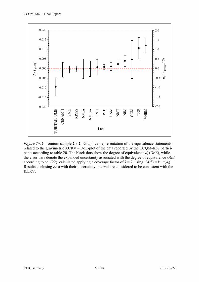
CCQM-K87 – Final Report
PTB, Germany 56/104 2012-05-22
TUBI
TAK
UM
E
CEN
AM
-1
SMU
KRI
SS
NM
IA
NM
ISA
INTI
PTB
BAM
NIS
T
NIM
GU
M
LNE
VN
IIM
-0.020
-0.015
-0.010
-0.005
0.000
0.005
0.010
0.015
0.020d i /
(g/k
g)
Lab
-2.0
-1.5
-1.0
-0.5
0.0
0.5
1.0
1.5
2.0
di /
wK
CR
V /
%
Figure 26: Chromium sample Cr-C. Graphical representation of the equivalence statements related to the gravimetric KCRV – DoE-plot of the data reported by the CCQM-K87 partici-pants according to table 20. The black dots show the degree of equivalence di (DoE), while the error bars denote the expanded uncertainty associated with the degree of equivalence U(di) according to eq. (22), calculated applying a coverage factor of k = 2, using U(di) = k · u(di). Results enclosing zero with their uncertainty interval are considered to be consistent with the KCRV.
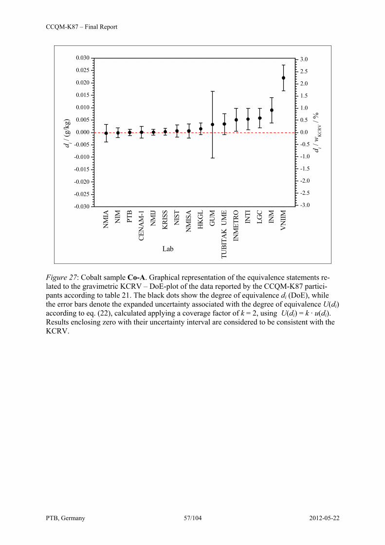
CCQM-K87 – Final Report
PTB, Germany 57/104 2012-05-22
NM
IA
NIM PT
B
CEN
AM
-1
NM
IJ
KRI
SS
NIS
T
NM
ISA
HK
GL
GU
M
TUBI
TAK
UM
E
INM
ETRO INTI
LGC
INM
VN
IIM
-0.030
-0.025
-0.020
-0.015
-0.010
-0.005
0.000
0.005
0.010
0.015
0.020
0.025
0.030d i /
(g/k
g)
Lab
-3.0
-2.5
-2.0
-1.5
-1.0
-0.5
0.0
0.5
1.0
1.5
2.0
2.5
3.0
di /
wK
CR
V /
%
Figure 27: Cobalt sample Co-A. Graphical representation of the equivalence statements re-lated to the gravimetric KCRV – DoE-plot of the data reported by the CCQM-K87 partici-pants according to table 21. The black dots show the degree of equivalence di (DoE), while the error bars denote the expanded uncertainty associated with the degree of equivalence U(di) according to eq. (22), calculated applying a coverage factor of k = 2, using U(di) = k · u(di). Results enclosing zero with their uncertainty interval are considered to be consistent with the KCRV.
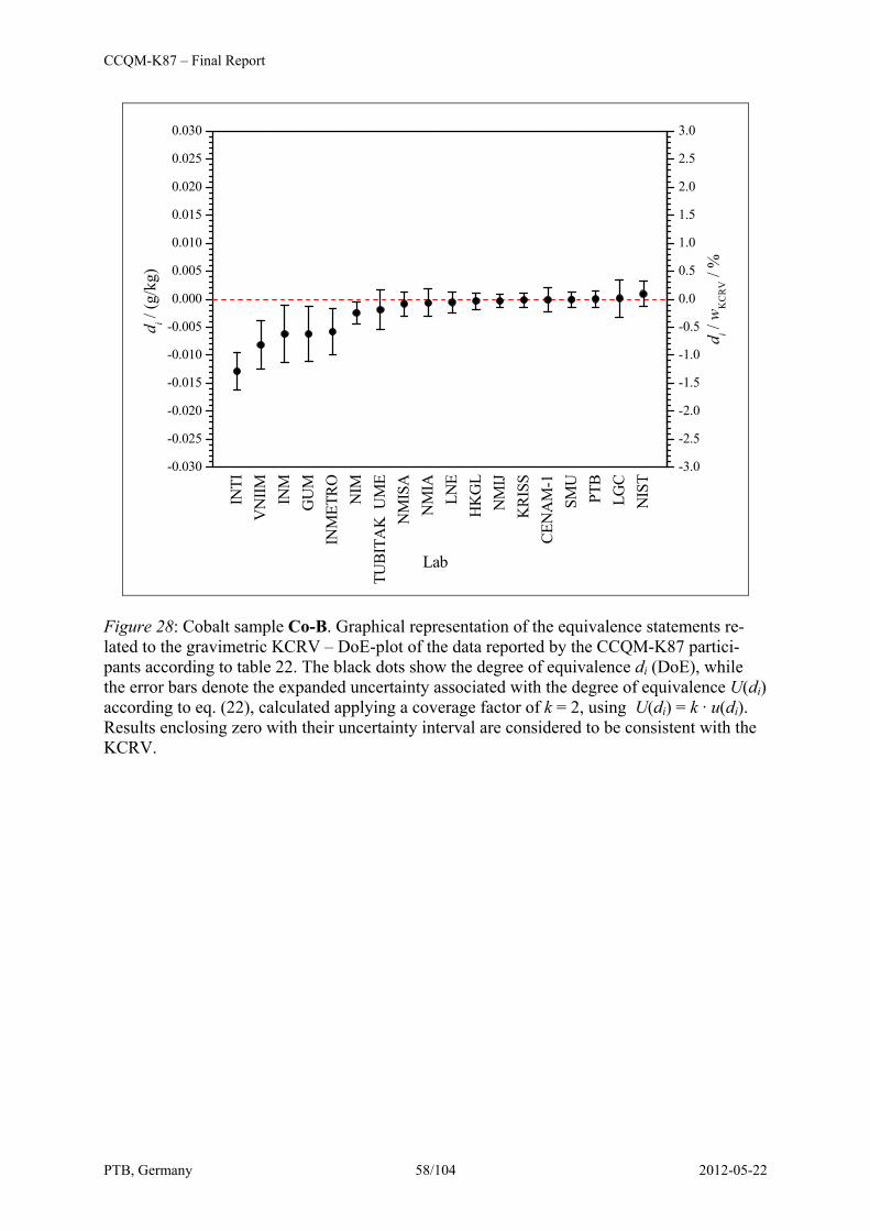
CCQM-K87 – Final Report
PTB, Germany 58/104 2012-05-22
INTI
VN
IIM INM
GU
MIN
MET
RO NIM
TUBI
TAK
UM
EN
MIS
AN
MIA
LNE
HK
GL
NM
IJK
RISS
CEN
AM
-1SM
UPT
BLG
CN
IST
-0.030
-0.025
-0.020
-0.015
-0.010
-0.005
0.000
0.005
0.010
0.015
0.020
0.025
0.030d i /
(g/k
g)
Lab
-3.0
-2.5
-2.0
-1.5
-1.0
-0.5
0.0
0.5
1.0
1.5
2.0
2.5
3.0
di /
wK
CR
V /
%
Figure 28: Cobalt sample Co-B. Graphical representation of the equivalence statements re-lated to the gravimetric KCRV – DoE-plot of the data reported by the CCQM-K87 partici-pants according to table 22. The black dots show the degree of equivalence di (DoE), while the error bars denote the expanded uncertainty associated with the degree of equivalence U(di) according to eq. (22), calculated applying a coverage factor of k = 2, using U(di) = k · u(di). Results enclosing zero with their uncertainty interval are considered to be consistent with the KCRV.
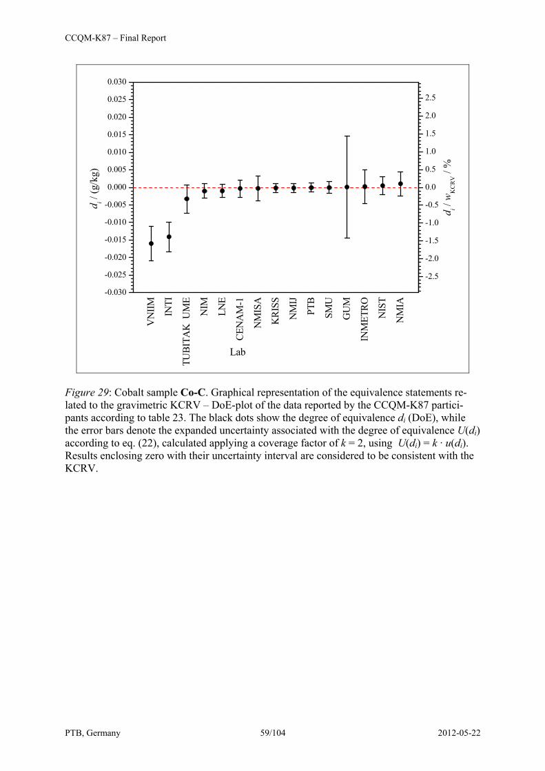
CCQM-K87 – Final Report
PTB, Germany 59/104 2012-05-22
VN
IIM INTI
TUBI
TAK
UM
E
NIM
LNE
CEN
AM
-1
NM
ISA
KRI
SS
NM
IJ
PTB
SMU
GU
M
INM
ETRO
NIS
T
NM
IA
-0.030
-0.025
-0.020
-0.015
-0.010
-0.005
0.000
0.005
0.010
0.015
0.020
0.025
0.030d i /
(g/k
g)
Lab
-2.5
-2.0
-1.5
-1.0
-0.5
0.0
0.5
1.0
1.5
2.0
2.5
di /
wK
CR
V /
%
Figure 29: Cobalt sample Co-C. Graphical representation of the equivalence statements re-lated to the gravimetric KCRV – DoE-plot of the data reported by the CCQM-K87 partici-pants according to table 23. The black dots show the degree of equivalence di (DoE), while the error bars denote the expanded uncertainty associated with the degree of equivalence U(di) according to eq. (22), calculated applying a coverage factor of k = 2, using U(di) = k · u(di). Results enclosing zero with their uncertainty interval are considered to be consistent with the KCRV.

CCQM-K87 – Final Report
PTB, Germany 60/104 2012-05-22
BAM
NM
IJ
PTB
LGC
NIM
KRI
SS
CEN
AM
-1
HK
GL
NIS
T
NM
IA
NM
ISA
INM
TUBI
TAK
UM
E
VN
IIM INTI
GU
M
-0.030
-0.025
-0.020
-0.015
-0.010
-0.005
0.000
0.005
0.010
0.015
0.020
0.025
0.030d i /
(g/k
g)
Lab
0.05
59
-3.0
-2.5
-2.0
-1.5
-1.0
-0.5
0.0
0.5
1.0
1.5
2.0
2.5
3.0
di /
wK
CR
V /
%
Figure 30: Lead sample Pb-A. Graphical representation of the equivalence statements related to the gravimetric KCRV – DoE-plot of the data reported by the CCQM-K87 participants according to table 24. The black dots show the degree of equivalence di (DoE), while the error bars denote the expanded uncertainty associated with the degree of equivalence U(di) accord-ing to eq. (22), calculated applying a coverage factor of k = 2, using U(di) = k · u(di). Results enclosing zero with their uncertainty interval are considered to be consistent with the KCRV.
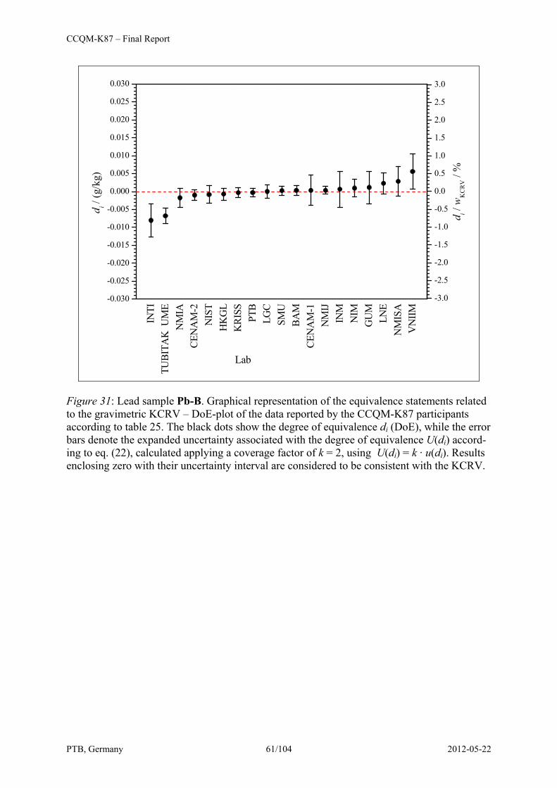
CCQM-K87 – Final Report
PTB, Germany 61/104 2012-05-22
INTI
TUBI
TAK
UM
EN
MIA
CEN
AM
-2N
IST
HK
GL
KRI
SSPT
BLG
CSM
UBA
MCE
NA
M-1
NM
IJIN
MN
IMG
UM
LNE
NM
ISA
VN
IIM
-0.030
-0.025
-0.020
-0.015
-0.010
-0.005
0.000
0.005
0.010
0.015
0.020
0.025
0.030d i /
(g/k
g)
Lab
-3.0
-2.5
-2.0
-1.5
-1.0
-0.5
0.0
0.5
1.0
1.5
2.0
2.5
3.0
di /
wK
CR
V /
%
Figure 31: Lead sample Pb-B. Graphical representation of the equivalence statements related to the gravimetric KCRV – DoE-plot of the data reported by the CCQM-K87 participants according to table 25. The black dots show the degree of equivalence di (DoE), while the error bars denote the expanded uncertainty associated with the degree of equivalence U(di) accord-ing to eq. (22), calculated applying a coverage factor of k = 2, using U(di) = k · u(di). Results enclosing zero with their uncertainty interval are considered to be consistent with the KCRV.
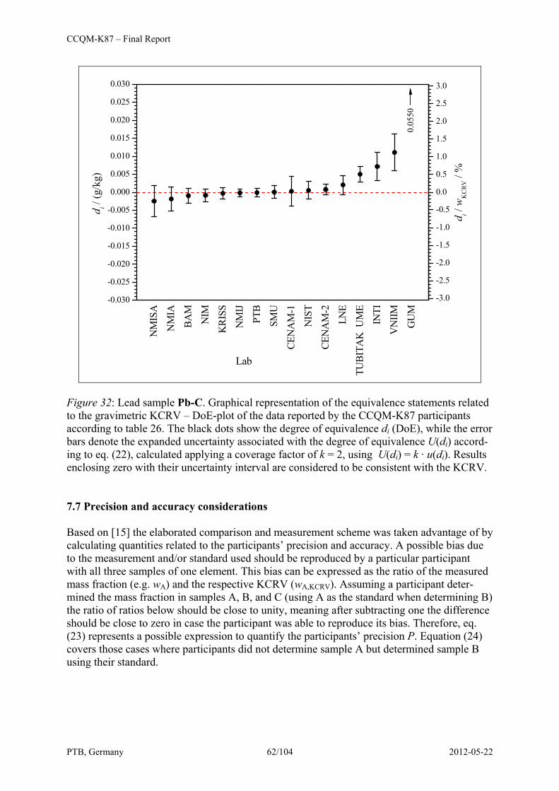
CCQM-K87 – Final Report
PTB, Germany 62/104 2012-05-22
NM
ISA
NM
IA
BAM
NIM
KRI
SS
NM
IJ
PTB
SMU
CEN
AM
-1
NIS
T
CEN
AM
-2
LNE
TUBI
TAK
UM
E
INTI
VN
IIM
GU
M
-0.030
-0.025
-0.020
-0.015
-0.010
-0.005
0.000
0.005
0.010
0.015
0.020
0.025
0.030d i /
(g/k
g)
Lab
0.05
50
-3.0
-2.5
-2.0
-1.5
-1.0
-0.5
0.0
0.5
1.0
1.5
2.0
2.5
3.0
di /
wK
CR
V /
%
Figure 32: Lead sample Pb-C. Graphical representation of the equivalence statements related to the gravimetric KCRV – DoE-plot of the data reported by the CCQM-K87 participants according to table 26. The black dots show the degree of equivalence di (DoE), while the error bars denote the expanded uncertainty associated with the degree of equivalence U(di) accord-ing to eq. (22), calculated applying a coverage factor of k = 2, using U(di) = k · u(di). Results enclosing zero with their uncertainty interval are considered to be consistent with the KCRV. 7.7 Precision and accuracy considerations Based on [15] the elaborated comparison and measurement scheme was taken advantage of by calculating quantities related to the participants’ precision and accuracy. A possible bias due to the measurement and/or standard used should be reproduced by a particular participant with all three samples of one element. This bias can be expressed as the ratio of the measured mass fraction (e.g. wA) and the respective KCRV (wA,KCRV). Assuming a participant deter-mined the mass fraction in samples A, B, and C (using A as the standard when determining B) the ratio of ratios below should be close to unity, meaning after subtracting one the difference should be close to zero in case the participant was able to reproduce its bias. Therefore, eq. (23) represents a possible expression to quantify the participants’ precision P. Equation (24) covers those cases where participants did not determine sample A but determined sample B using their standard.

CCQM-K87 – Final Report
PTB, Germany 63/104 2012-05-22
01
KCRVA,
A
KCRVC,
C
→−=
ww
ww
P (23)
01
KCRVB,
B
KCRVC,
C
→−=
ww
ww
P (24)
Assuming all participants measured with perfect precision and the KCRV is completely accu-rate the accuracy of the participants own standards can be retrieved from the reported data applying eq. (25). The result A of eq. (25) expresses the relative deviation of a participant’s standard from the respective KCRV that was used to determine sample A. For details refer to appendix D. The use of eq. (25) is limited to those participants who measured sample A as well as B, and at the same time used sample A as the standard when measuring sample B.
01
KCRVB,
B
KCRVA,
defA,
KCRVA,
A
→−⋅
=
ww
ww
ww
A (25)
Table 27–29 and figures 33–35 show the precision P and accuracy A according to the above equations. To draw conclusions from these data is complex and restricted to those cases where both P and A is available and additionally P is considerably smaller than A.
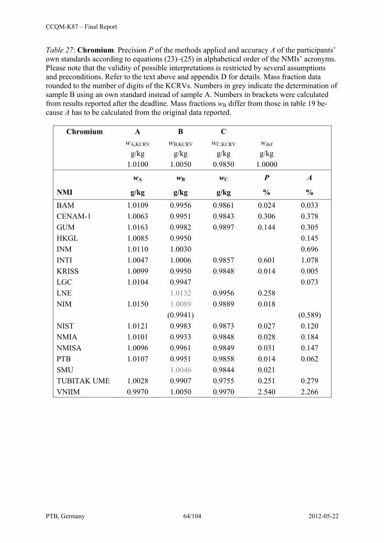
CCQM-K87 – Final Report
PTB, Germany 64/104 2012-05-22
Table 27: Chromium. Precision P of the methods applied and accuracy A of the participants’ own standards according to equations (23)–(25) in alphabetical order of the NMIs’ acronyms. Please note that the validity of possible interpretations is restricted by several assumptions and preconditions. Refer to the text above and appendix D for details. Mass fraction data rounded to the number of digits of the KCRVs. Numbers in grey indicate the determination of sample B using an own standard instead of sample A. Numbers in brackets were calculated from results reported after the deadline. Mass fractions wB differ from those in table 19 be-cause A has to be calculated from the original data reported.
Chromium A B C
wA,KCRV wB,KCRV wC,KCRV wdef g/kg g/kg g/kg g/kg 1.0100 1.0050 0.9850 1.0000
wA wB wC P A
NMI g/kg g/kg g/kg % %
BAM 1.0109 0.9956 0.9861 0.024 0.033 CENAM-1 1.0063 0.9951 0.9843 0.306 0.378 GUM 1.0163 0.9982 0.9897 0.144 0.305 HKGL 1.0085 0.9950 0.145 INM 1.0110 1.0030 0.696 INTI 1.0047 1.0006 0.9857 0.601 1.078 KRISS 1.0099 0.9950 0.9848 0.014 0.005 LGC 1.0104 0.9947 0.073 LNE 1.0132 0.9956 0.258 NIM 1.0150 1.0089 0.9889 0.018 (0.9941) (0.589) NIST 1.0121 0.9983 0.9873 0.027 0.120 NMIA 1.0101 0.9933 0.9848 0.028 0.184 NMISA 1.0096 0.9961 0.9849 0.031 0.147 PTB 1.0107 0.9951 0.9858 0.014 0.062 SMU 1.0046 0.9844 0.021 TUBITAK UME 1.0028 0.9907 0.9755 0.251 0.279 VNIIM 0.9970 1.0050 0.9970 2.540 2.266
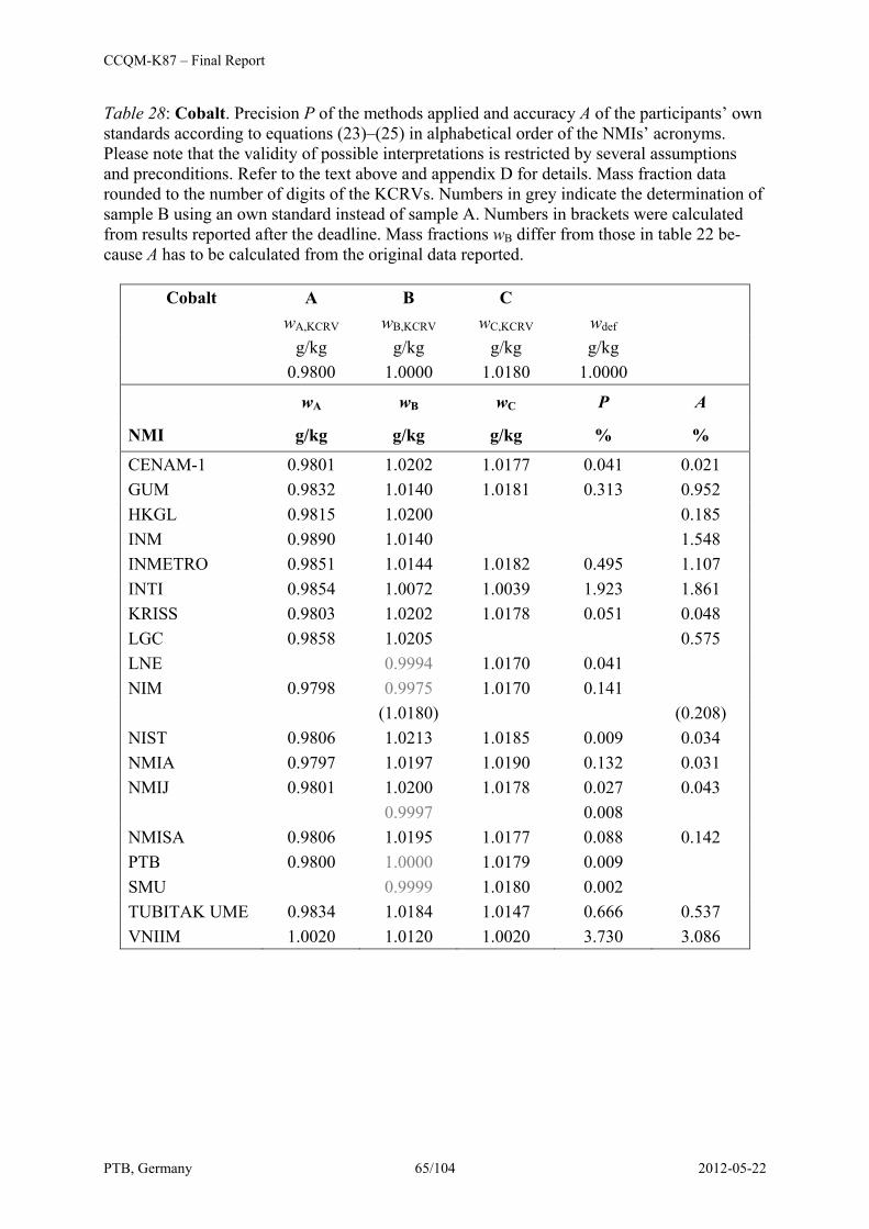
CCQM-K87 – Final Report
PTB, Germany 65/104 2012-05-22
Table 28: Cobalt. Precision P of the methods applied and accuracy A of the participants’ own standards according to equations (23)–(25) in alphabetical order of the NMIs’ acronyms. Please note that the validity of possible interpretations is restricted by several assumptions and preconditions. Refer to the text above and appendix D for details. Mass fraction data rounded to the number of digits of the KCRVs. Numbers in grey indicate the determination of sample B using an own standard instead of sample A. Numbers in brackets were calculated from results reported after the deadline. Mass fractions wB differ from those in table 22 be-cause A has to be calculated from the original data reported.
Cobalt A B C
wA,KCRV wB,KCRV wC,KCRV wdef g/kg g/kg g/kg g/kg 0.9800 1.0000 1.0180 1.0000
wA wB wC P A
NMI g/kg g/kg g/kg % %
CENAM-1 0.9801 1.0202 1.0177 0.041 0.021 GUM 0.9832 1.0140 1.0181 0.313 0.952 HKGL 0.9815 1.0200 0.185 INM 0.9890 1.0140 1.548 INMETRO 0.9851 1.0144 1.0182 0.495 1.107 INTI 0.9854 1.0072 1.0039 1.923 1.861 KRISS 0.9803 1.0202 1.0178 0.051 0.048 LGC 0.9858 1.0205 0.575 LNE 0.9994 1.0170 0.041 NIM 0.9798 0.9975 1.0170 0.141 (1.0180) (0.208) NIST 0.9806 1.0213 1.0185 0.009 0.034 NMIA 0.9797 1.0197 1.0190 0.132 0.031 NMIJ 0.9801 1.0200 1.0178 0.027 0.043 0.9997 0.008 NMISA 0.9806 1.0195 1.0177 0.088 0.142 PTB 0.9800 1.0000 1.0179 0.009 SMU 0.9999 1.0180 0.002 TUBITAK UME 0.9834 1.0184 1.0147 0.666 0.537 VNIIM 1.0020 1.0120 1.0020 3.730 3.086
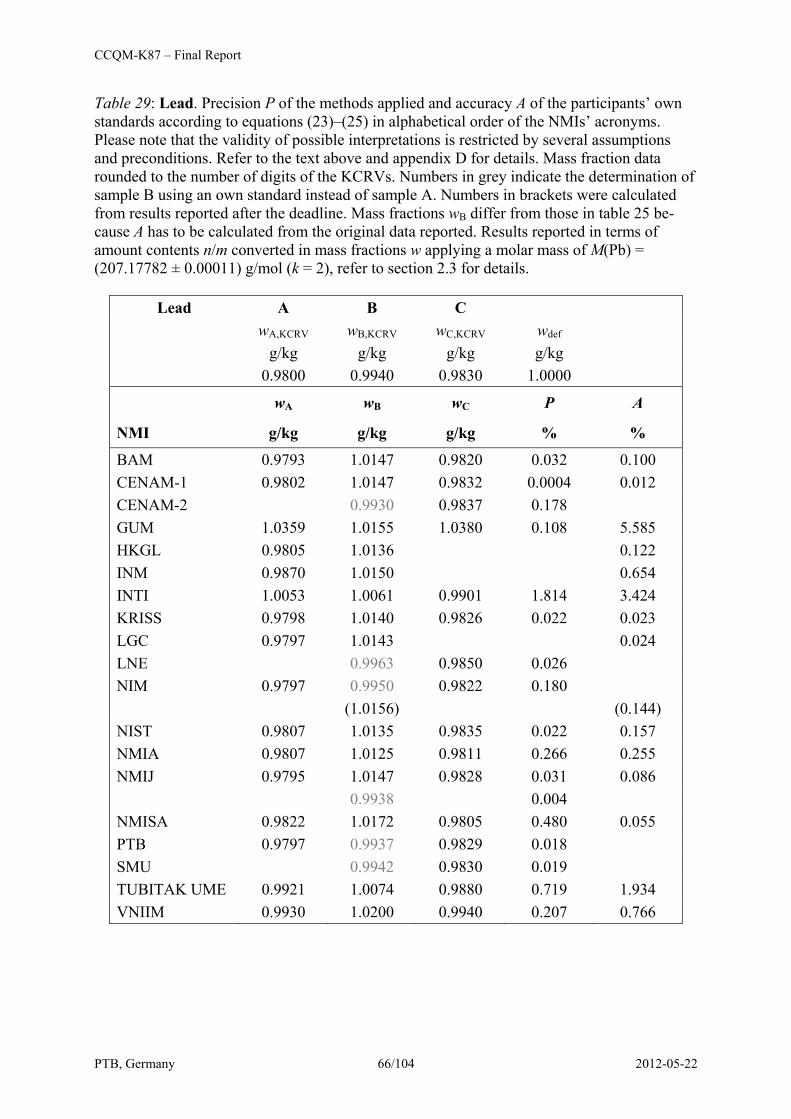
CCQM-K87 – Final Report
PTB, Germany 66/104 2012-05-22
Table 29: Lead. Precision P of the methods applied and accuracy A of the participants’ own standards according to equations (23)–(25) in alphabetical order of the NMIs’ acronyms. Please note that the validity of possible interpretations is restricted by several assumptions and preconditions. Refer to the text above and appendix D for details. Mass fraction data rounded to the number of digits of the KCRVs. Numbers in grey indicate the determination of sample B using an own standard instead of sample A. Numbers in brackets were calculated from results reported after the deadline. Mass fractions wB differ from those in table 25 be-cause A has to be calculated from the original data reported. Results reported in terms of amount contents n/m converted in mass fractions w applying a molar mass of M(Pb) = (207.17782 ± 0.00011) g/mol (k = 2), refer to section 2.3 for details.
Lead A B C
wA,KCRV wB,KCRV wC,KCRV wdef g/kg g/kg g/kg g/kg 0.9800 0.9940 0.9830 1.0000
wA wB wC P A
NMI g/kg g/kg g/kg % %
BAM 0.9793 1.0147 0.9820 0.032 0.100 CENAM-1 0.9802 1.0147 0.9832 0.0004 0.012 CENAM-2 0.9930 0.9837 0.178 GUM 1.0359 1.0155 1.0380 0.108 5.585 HKGL 0.9805 1.0136 0.122 INM 0.9870 1.0150 0.654 INTI 1.0053 1.0061 0.9901 1.814 3.424 KRISS 0.9798 1.0140 0.9826 0.022 0.023 LGC 0.9797 1.0143 0.024 LNE 0.9963 0.9850 0.026 NIM 0.9797 0.9950 0.9822 0.180 (1.0156) (0.144) NIST 0.9807 1.0135 0.9835 0.022 0.157 NMIA 0.9807 1.0125 0.9811 0.266 0.255 NMIJ 0.9795 1.0147 0.9828 0.031 0.086 0.9938 0.004 NMISA 0.9822 1.0172 0.9805 0.480 0.055 PTB 0.9797 0.9937 0.9829 0.018 SMU 0.9942 0.9830 0.019 TUBITAK UME 0.9921 1.0074 0.9880 0.719 1.934 VNIIM 0.9930 1.0200 0.9940 0.207 0.766
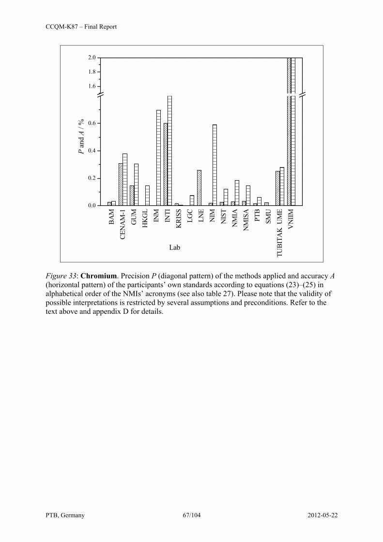
CCQM-K87 – Final Report
PTB, Germany 67/104 2012-05-22
BAM
CEN
AM
-1G
UM
HK
GL
INM
INTI
KRI
SSLG
CLN
EN
IMN
IST
NM
IAN
MIS
APT
BSM
UTU
BITA
K U
ME
VN
IIM
0.0
0.2
0.4
0.6
1.6
1.8
2.0
P an
d A
/ %
Lab
Figure 33: Chromium. Precision P (diagonal pattern) of the methods applied and accuracy A (horizontal pattern) of the participants’ own standards according to equations (23)–(25) in alphabetical order of the NMIs’ acronyms (see also table 27). Please note that the validity of possible interpretations is restricted by several assumptions and preconditions. Refer to the text above and appendix D for details.

CCQM-K87 – Final Report
PTB, Germany 68/104 2012-05-22
CEN
AM
-1G
UM
HK
GL
INM
INM
ETRO INTI
KRI
SSLG
CLN
EN
IMN
IST
NM
IAN
MIJ
NM
ISA
PTB
SMU
TUBI
TAK
UM
EV
NIIM
0.0
0.2
0.4
0.6
1.6
1.8
2.0
P an
d A
/ %
Lab
Figure 34: Cobalt. Precision P (diagonal pattern) of the methods applied and accuracy A (horizontal pattern) of the participants’ own standards according to equations (23)–(25) in alphabetical order of the NMIs’ acronyms (see also table 28). Please note that the validity of possible interpretations is restricted by several assumptions and preconditions. Refer to the text above and appendix D for details.
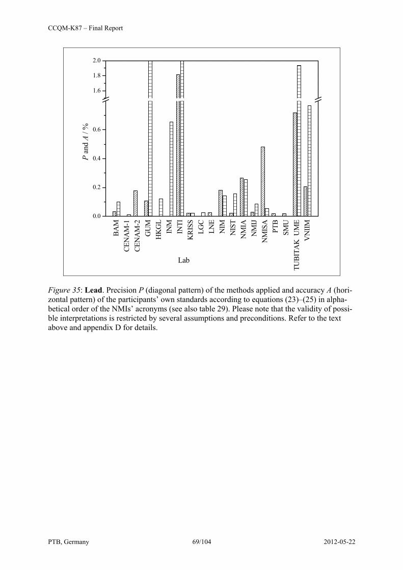
CCQM-K87 – Final Report
PTB, Germany 69/104 2012-05-22
BAM
CEN
AM
-1CE
NA
M-2
GU
MH
KG
LIN
MIN
TIK
RISS
LGC
LNE
NIM
NIS
TN
MIA
NM
IJN
MIS
APT
BSM
UTU
BITA
K U
ME
VN
IIM
0.0
0.2
0.4
0.6
1.6
1.8
2.0
P an
d A
/ %
Lab
Figure 35: Lead. Precision P (diagonal pattern) of the methods applied and accuracy A (hori-zontal pattern) of the participants’ own standards according to equations (23)–(25) in alpha-betical order of the NMIs’ acronyms (see also table 29). Please note that the validity of possi-ble interpretations is restricted by several assumptions and preconditions. Refer to the text above and appendix D for details.
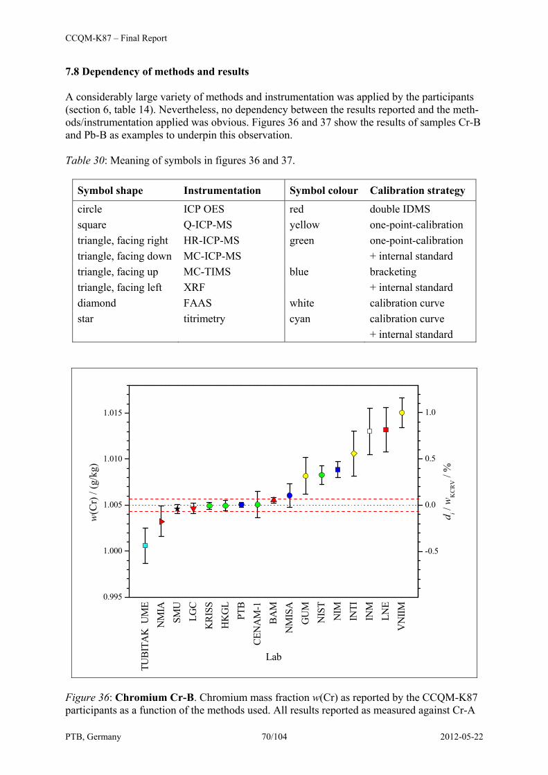
CCQM-K87 – Final Report
PTB, Germany 70/104 2012-05-22
7.8 Dependency of methods and results A considerably large variety of methods and instrumentation was applied by the participants (section 6, table 14). Nevertheless, no dependency between the results reported and the meth-ods/instrumentation applied was obvious. Figures 36 and 37 show the results of samples Cr-B and Pb-B as examples to underpin this observation. Table 30: Meaning of symbols in figures 36 and 37.
Symbol shape Instrumentation Symbol colour Calibration strategy
circle ICP OES red double IDMS square Q-ICP-MS yellow one-point-calibration triangle, facing right HR-ICP-MS green one-point-calibration triangle, facing down MC-ICP-MS + internal standard triangle, facing up MC-TIMS blue bracketing triangle, facing left XRF + internal standard diamond FAAS white calibration curve star titrimetry cyan calibration curve + internal standard
TUBI
TAK
UM
EN
MIA
SMU
LGC
KRI
SSH
KG
LPT
BCE
NA
M-1
BAM
NM
ISA
GU
MN
IST
NIM
INTI
INM
LNE
VN
IIM
0.995
1.000
1.005
1.010
1.015
w(C
r) /
(g/k
g)
Lab
-0.5
0.0
0.5
1.0
di /
wK
CR
V /
%
Figure 36: Chromium Cr-B. Chromium mass fraction w(Cr) as reported by the CCQM-K87 participants as a function of the methods used. All results reported as measured against Cr-A
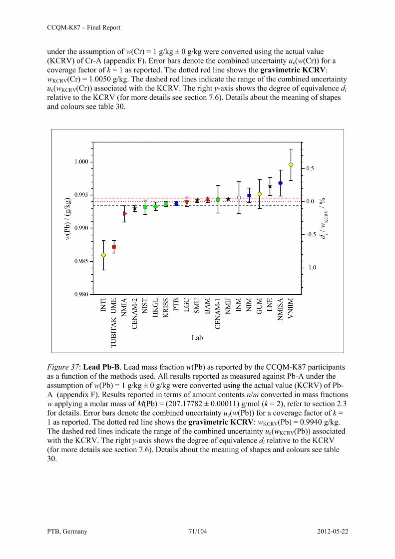
CCQM-K87 – Final Report
PTB, Germany 71/104 2012-05-22
under the assumption of w(Cr) = 1 g/kg ± 0 g/kg were converted using the actual value (KCRV) of Cr-A (appendix F). Error bars denote the combined uncertainty uc(w(Cr)) for a coverage factor of k = 1 as reported. The dotted red line shows the gravimetric KCRV: wKCRV(Cr) = 1.0050 g/kg. The dashed red lines indicate the range of the combined uncertainty uc(wKCRV(Cr)) associated with the KCRV. The right y-axis shows the degree of equivalence di relative to the KCRV (for more details see section 7.6). Details about the meaning of shapes and colours see table 30.
INTI
TUBI
TAK
UM
EN
MIA
CEN
AM
-2N
IST
HK
GL
KRI
SSPT
BLG
CSM
UBA
MCE
NA
M-1
NM
IJIN
MN
IMG
UM
LNE
NM
ISA
VN
IIM0.980
0.985
0.990
0.995
1.000
w(P
b) /
(g/k
g)
Lab
-1.0
-0.5
0.0
0.5
di /
wK
CR
V /
%
Figure 37: Lead Pb-B. Lead mass fraction w(Pb) as reported by the CCQM-K87 participants as a function of the methods used. All results reported as measured against Pb-A under the assumption of w(Pb) = 1 g/kg ± 0 g/kg were converted using the actual value (KCRV) of Pb-A (appendix F). Results reported in terms of amount contents n/m converted in mass fractions w applying a molar mass of M(Pb) = (207.17782 ± 0.00011) g/mol (k = 2), refer to section 2.3 for details. Error bars denote the combined uncertainty uc(w(Pb)) for a coverage factor of k = 1 as reported. The dotted red line shows the gravimetric KCRV: wKCRV(Pb) = 0.9940 g/kg. The dashed red lines indicate the range of the combined uncertainty uc(wKCRV(Pb)) associated with the KCRV. The right y-axis shows the degree of equivalence di relative to the KCRV (for more details see section 7.6). Details about the meaning of shapes and colours see table 30.
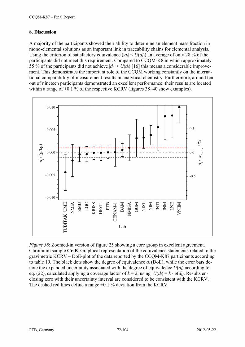
CCQM-K87 – Final Report
PTB, Germany 72/104 2012-05-22
8. Discussion A majority of the participants showed their ability to determine an element mass fraction in mono-elemental solutions as an important link in traceability chains for elemental analysis. Using the criterion of satisfactory equivalence (|di| < U(di)) an average of only 28 % of the participants did not meet this requirement. Compared to CCQM-K8 in which approximately 55 % of the participants did not achieve |di| < U(di) [16] this means a considerable improve-ment. This demonstrates the important role of the CCQM working constantly on the interna-tional comparability of measurement results in analytical chemistry. Furthermore, around ten out of nineteen participants demonstrated an excellent performance: their results are located within a range of ±0.1 % of the respective KCRV (figures 38–40 show examples).
TUBI
TAK
UM
EN
MIA
SMU
LGC
KRI
SSH
KG
LPT
BCE
NA
M-1
BAM
NM
ISA
GU
MN
IST
NIM
INTI
INM
LNE
VN
IIM
-0.010
-0.005
0.000
0.005
0.010
d i / (g
/kg)
Lab
-0.5
0.0
0.5
di /
wK
CR
V /
%
Figure 38: Zoomed-in version of figure 25 showing a core group in excellent agreement. Chromium sample Cr-B. Graphical representation of the equivalence statements related to the gravimetric KCRV – DoE-plot of the data reported by the CCQM-K87 participants according to table 19. The black dots show the degree of equivalence di (DoE), while the error bars de-note the expanded uncertainty associated with the degree of equivalence U(di) according to eq. (22), calculated applying a coverage factor of k = 2, using U(di) = k · u(di). Results en-closing zero with their uncertainty interval are considered to be consistent with the KCRV. The dashed red lines define a range ±0.1 % deviation from the KCRV.

CCQM-K87 – Final Report
PTB, Germany 73/104 2012-05-22
VN
IIM INTI
TUBI
TAK
UM
E
NIM
LNE
CEN
AM
-1
NM
ISA
KRI
SS
NM
IJ
PTB
SMU
GU
M
INM
ETRO
NIS
T
NM
IA
-0.010
-0.005
0.000
0.005
0.010d i /
(g/k
g)
Lab
-0.0
14
-0.0
16
-0.5
0.0
0.5
di /
wK
CR
V /
%
Figure 39: Zoomed-in version of figure 29 showing a core group in excellent agreement. Co-balt sample Co-C. Graphical representation of the equivalence statements related to the gra-vimetric KCRV – DoE-plot of the data reported by the CCQM-K87 participants according to table 23. The black dots show the degree of equivalence di (DoE), while the error bars denote the expanded uncertainty associated with the degree of equivalence U(di) according to eq. (22), calculated applying a coverage factor of k = 2, using U(di) = k · u(di). Results enclosing zero with their uncertainty interval are considered to be consistent with the KCRV. The dashed red lines define a range ±0.1 % deviation from the KCRV.
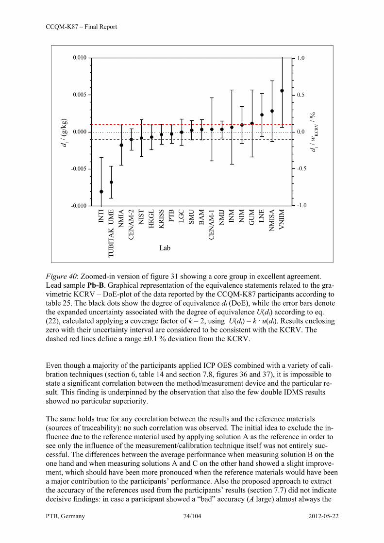
CCQM-K87 – Final Report
PTB, Germany 74/104 2012-05-22
INTI
TUBI
TAK
UM
EN
MIA
CEN
AM
-2N
IST
HK
GL
KRI
SSPT
BLG
CSM
UBA
MCE
NA
M-1
NM
IJIN
MN
IMG
UM
LNE
NM
ISA
VN
IIM
-0.010
-0.005
0.000
0.005
0.010d i /
(g/k
g)
Lab
-1.0
-0.5
0.0
0.5
1.0
di /
wK
CR
V /
%
Figure 40: Zoomed-in version of figure 31 showing a core group in excellent agreement. Lead sample Pb-B. Graphical representation of the equivalence statements related to the gra-vimetric KCRV – DoE-plot of the data reported by the CCQM-K87 participants according to table 25. The black dots show the degree of equivalence di (DoE), while the error bars denote the expanded uncertainty associated with the degree of equivalence U(di) according to eq. (22), calculated applying a coverage factor of k = 2, using U(di) = k · u(di). Results enclosing zero with their uncertainty interval are considered to be consistent with the KCRV. The dashed red lines define a range ±0.1 % deviation from the KCRV. Even though a majority of the participants applied ICP OES combined with a variety of cali-bration techniques (section 6, table 14 and section 7.8, figures 36 and 37), it is impossible to state a significant correlation between the method/measurement device and the particular re-sult. This finding is underpinned by the observation that also the few double IDMS results showed no particular superiority. The same holds true for any correlation between the results and the reference materials (sources of traceability): no such correlation was observed. The initial idea to exclude the in-fluence due to the reference material used by applying solution A as the reference in order to see only the influence of the measurement/calibration technique itself was not entirely suc-cessful. The differences between the average performance when measuring solution B on the one hand and when measuring solutions A and C on the other hand showed a slight improve-ment, which should have been more pronouced when the reference materials would have been a major contribution to the participants’ performance. Also the proposed approach to extract the accuracy of the references used from the participants’ results (section 7.7) did not indicate decisive findings: in case a participant showed a “bad” accuracy (A large) almost always the
CCQM-K87 – Final Report
PTB, Germany 75/104 2012-05-22
precison P was in the same order of magnitude which prevents any conclusion. On the other hand participants showing a sufficient precison P almost always shined with a small A. Even though this comparison is fortunately supported by a considerably large amount of data, this amount is insufficient to resolve such a delicate issue as possible differences of the references used. The parallel pilot study CCQM-P124 (appendix C) demonstrated that at least the participating two industry laboratories (both supplier of secondary calibration solutions) are able to suc-cessfully measure mono-elemental calibration solutions on par with the majority of NMIs. This is an encouraging finding because the traceability in the field is usually achieved via secondary calibration solutions from manufacturers like the ones who participated. This report includes no core competencies tables due to the clear and narrow range of compe-tencies demonstrated and the absence of a complex and/or challenging matrix. Median and uncertainty weighted mean KCRV estimators were in excellent agreement with the proposed gravimetric KCRVs (derived from the sample preparation). The average relative deviation of the median and uncertainty weighted mean KCRV estimators from the gravimet-ric KCRV was 0.05 % and 0.03 %, respectively. The KCRVs were accepted by the IAWG during the Sydney meeting on 1 November 2011. Therefore, this comparison was successfully completed.
CCQM-K87 – Final Report
PTB, Germany 76/104 2012-05-22
9. References [1] CCQM Inorganic Analysis Working Group, Minutes of the meeting held on 1-4 Novem-
ber 2011, NMIA, Sydney, Australia. http://www.bipm.org/wg/CCQM/IAWG/Restricted/welcome.jsp
[2] Heinrich Kipphardt, Ralf Matschat, Olaf Rienitz, Detlef Schiel, Wolfgang Gernand, Dietmar Oeter, Traceability system for elemental analysis, Accred Qual Assur (2006) 10: 633-639
[3] Heinrich Kipphardt, Ralf Matschat, Purity assessment for providing primary standards for elemental determination – a snap shot of international comparability, Microchim Acta (2008) 162: 269-275
[4] Heinrich Kipphardt, Ralf Matschat, Jochen Vogl, Tamara Gusarova, Michael Czerwen-sky, Hans-Joachim Heinrich, Akiharu Hioki, Leonid A. Konopelko, Brad Methven, Tsu-tomu Miura, Ole Petersen, Gundel Riebe, Ralph Sturgeon, Gregory C. Turk, Lee L. Yu, Purity determination as needed for the realisation of primary standards for elemental de-termination: status of international comparability, Accred Qual Assur (2010) 15:29–37
[5] Anna-Lisa Hauswaldt, Olaf Rienitz, Reinhard Jährling, Nicolas Fischer, Detlef Schiel, Guillaume Labarraque, Bertil Magnusson, Uncertainty of standard addition experiments: a novel approach to include the uncertainty associated with the standard in the model equation, Accred Qual Assur (2011) doi:10.1007/s00769-011-0827-5.
[6] ISO Guide 35, Reference materials — General and statistical principles for certification, 3rd edition, International Organization for Standardization, Geneva, 2006.
[7] Evaluation of measurement data - Guide to the expression of uncertainty in measure-ment, JCGM 100:2008. http://www.bipm.org/utils/common/documents/jcgm/JCGM_100_2008_E.pdf
[8] CCQM Guidance note: Estimation of a consensus KCRV and associated Degrees of Equivalence, Version 6, 2010-03-01, Draft.
[9] Wolfgang Gottwald, Statistik für Anwender, WILEY-VCH, Weinheim, 2000. [10] W. J. Dixon, Analysis of extreme values, The Annals of Mathematical Statistics 21, 4
(1950), 488-506. [11] W. J. Dixon, Processing data for outliers, J Biometrics 9 (1953) 74-89. [12] R. B. Dean, W. J. Dixon, Simplified statistics for small numbers of observations, Ana-
lytical Chemistry 23 (1951) 636-638. [13] Lothar Sachs, Angewandte Statistik, Springer, Berlin, 1997. [14] Dieter Richter, Wolfgang Wöger, Werner Hässelbarth (eds.), Data analysis of key
comparisons, Braunschweig and Berlin, 2003, ISBN 3-89701-933-3. [15] Michal Máriássy, personal communication, November 2011. [16] Helene Felber, Michael Weber, Cédric Rivier, CCQM-K8 Key Comparison —
Monoelemental Calibration Solutions, Metrologia, 2002, 39, Tech. Suppl., 08002

CCQM-K87 / CCQM-P124 Appendix A
PTB, Germany 77/104 2010-12-07
Physikalisch-Technische Bundesanstalt
Braunschweig und Berlin
CCQM-K87 and CCQM-P124
“Mono-elemental Calibration Solutions”
Technical Protocol 1. Introduction Mono-elemental solutions are required for calibration purposes in elemental analysis and are therefore a prerequisite for reliable measurement results. This key comparison and the parallel pilot study address the particular importance of mono-elemental solutions. Cr, Co and Pb were carefully selected as the analytes. The comparisons are part of the broader context of “Traceability in elemental analysis” implemented with the aid of CCQM-P62, CCQM-P107, and CCQM-K72 (characterisation of impurities in pure substances serving as the traceability basis) as well as CCQM-P46 (preparation of primary elemental calibration solutions) and CCQM-K8 (determination of the element content in primary calibration solutions). The comparisons CCQM-K87 and CCQM-P124 are follow-ups of the key comparison CCQM-K8 (conducted in 2000) which was concerned with elemental solutions of Al, Cu, Fe and Mg. National metrology institutes and designated institutes were invited to participate in CCQM-K87 in order to confirm existing CMC claims or to facilitate the application of new CMC claims. 2. Samples Nine mono-elemental solutions were prepared gravimetrically at PTB starting from the German national standards provided by BAM (cobalt and lead) and from a primary material provided by CENAM (chromium), respectively. The following table summarizes these solutions and shows the notation used:
type of solution chromium cobalt lead
A – calibration solution Cr-A Co-A Pb-A
B – sample solution Cr-B Co-B Pb-B
C – “commercial” sample solution Cr-C Co-C Pb-C
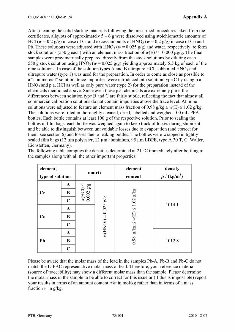
CCQM-K87 / CCQM-P124 Appendix A
PTB, Germany 78/104 2010-12-07
After cleaning the solid starting materials following the prescribed procedures taken from the certificates, aliquots of approximately 5 – 6 g were dissolved using stoichiometric amounts of HCl (w = 0.2 g/g) in case of Cr and excess amounts of HNO3 (w = 0.2 g/g) in case of Co and Pb. These solutions were adjusted with HNO3 (w = 0.025 g/g) and water, respectively, to form stock solutions (550 g each) with an element mass fraction of w(E) ≈ 10 000 µg/g. The final samples were gravimetrically prepared directly from the stock solutions by diluting each 550 g stock solution using HNO3 (w = 0.025 g/g) yielding approximately 5.5 kg of each of the nine solutions. In case of the solution types A and B ultrapure HCl, subboiled HNO3 and ultrapure water (type 1) was used for the preparation. In order to come as close as possible to a “commercial” solution, trace impurities were introduced into solution type C by using p.a. HNO3 and p.a. HCl as well as only pure water (type 2) for the preparation instead of the chemicals mentioned above. Since even these p.a. chemicals are extremely pure, the differences between solution type B and C are fairly subtle, reflecting the fact that almost all commercial calibration solutions do not contain impurities above the trace level. All nine solutions were adjusted to feature an element mass fraction of 0.98 g/kg ≤ w(E) ≤ 1.02 g/kg. The solutions were filled in thoroughly cleaned, dried, labelled and weighed 100 mL-PFA bottles. Each bottle contains at least 100 g of the respective solution. Prior to sealing the bottles in film bags, each bottle was weighed again to keep track of losses during shipment and be able to distinguish between unavoidable losses due to evaporation (and correct for them, see section 6) and losses due to leaking bottles. The bottles were wrapped in tightly sealed film bags (12 µm polyester, 12 µm aluminium, 95 µm LDPE, type A 30 T, C. Waller, Eichstetten, Germany). The following table compiles the densities determined at 21 °C immediately after bottling of the samples along with all the other important properties:
element,
type of solution matrix
element
content
density
ρ / (kg/m3)
Cr
A
w(H
Cl)
< 0.
002
g/g
w(H
NO
3) ≈
0.0
25 g
/g
0.98
g/k
g ≤
w(E
) ≤ 1
.02
g/kg
1014.1
B
C
Co
A
B
C
Pb
A
1012.8 B
C Please be aware that the molar mass of the lead in the samples Pb-A, Pb-B and Pb-C do not match the IUPAC representative molar mass of lead. Therefore, your reference material (source of traceability) may show a different molar mass than the sample. Please determine the molar mass in the sample to be able to correct for this issue or (if this is impossible) report your results in terms of an amount content n/m in mol/kg rather than in terms of a mass fraction w in g/kg.
CCQM-K87 / CCQM-P124 Appendix A
PTB, Germany 79/104 2010-12-07
3. Sample handling Before opening the bags, please be prepared to weigh the bottles and to measure the ambient conditions (air pressure, air temperature, and relative humidity of the air). Please weigh the bottles immediately after opening the bags. Weigh them together with their screw-caps and labels. Please calculate possible losses according to section 6. 4. Analysis Please apply your most accurate methods of measurement, preferably primary methods. Note that the relative expanded measurement uncertainty Urel associated with your result must not exceed 0.5 % as already announced in the invitation. You are asked to determine the following quantities:
• Mass fraction wA(E) of the element E in solution A based on your own standard. • Mass fraction wB(E) of the element E in solution B using the provided calibration • solution A while assuming that its mass fraction is exactly wA(E) = 1 g/kg. • Mass fraction wC(E) of the element E in solution C based on your own standard. • In case you intend to use titrimetry, please determine wB(E) and wC(E) based on your
own standard. • In case you do not use titrimetry, the determination of wC(E) is voluntary, but every
result would be appreciated very much. 5. Reporting Note that the reporting deadline has been changed. The new deadline for the submission of results is 15 March 2011. Please send your report via E-mail. Please report all your results in terms of a mass fraction w in g/kg. Since it is necessary for the measurement of the lead samples, please determine and report also the molar mass of the lead M(Pb) in the lead samples along with the amount fraction x(iPb) in mol/mol of all the lead isotopes. Participants without the opportunity to determine the molar mass of the lead in the lead samples should report the lead results in terms of an amount content n(Pb)/m in mol/kg. Please report also all the masses of all solutions at the time of opening the bottles for the first time. Please refer to section 6 to do this. Please calculate uncertainties for all the results reported according to the GUM [1]. Please, report also your sources of traceability along with a short description of the method(s) you used. If you need further assistance or encounter any kind of problem, please contact Detlef Schiel and/or Olaf Rienitz. Contact: Dr. Detlef Schiel Dr. Olaf Rienitz Physikalisch-Technische Bundesanstalt Bundesallee 100 38116 Braunschweig Germany Fax +49-531-592-3015 Phone +49-531-592-3110 -3318 E-Mail [email protected] [email protected]

CCQM-K87 / CCQM-P124 Appendix A
PTB, Germany 80/104 2010-12-07
6. Checking for losses / correcting evaporation effects In addition to this “Technical Protocol” you should have received a table summarizing all bottles enclosed in your parcel together with the masses of the empty bottles mbottle and the masses of the solutions in these bottles msolution.
These masses were determined from the apparent masses (weighing values) of the empty bottle m1 and the bottle containing the according solution m2 determined at a time t1 and t2, respectively. Since the ambient conditions (relative humidity of the air ϕ, air pressure p and air temperature ϑ) were different at these times (t1 and t2), according air buoyancy correction factors Ki, j depending on the time j and the density of the weighed material i (PFA in case of the bottle, ρbottle, and the different solutions, ρsolution) were calculated to convert the apparent masses m1 and m2 into the masses mbottle and msolution.
2
32
3
22
3
2,air
solution
2,air
cal
2,air
solution,2
bottle
2,air
cal
2,air
bottle,2
bottle,2
bottle2solution,2solution
1
31
3
11
3
1,air
bottle
1,air
cal
1,air
bottle,1
1bottle,1bottle
C115.273
mkg0582.2
Cm/kg252.0
hPam/kg34844.0
1
1and
1
1
C115.273
mkg0582.2
Cm/kg252.0
hPam/kg34844.0
1
1
ϑ
ϑϕρ
ρρρρ
ρρρρ
ϑ
ϑϕρ
ρρρρ
⋅°
+
⎟⎟⎠
⎞⎜⎜⎝
⎛−⋅
°⋅−⋅
=
−
−=
−
−=
⎟⎟⎠
⎞⎜⎜⎝
⎛−⋅=
⋅°
+
⎟⎟⎠
⎞⎜⎜⎝
⎛−⋅
°⋅−⋅
=
−
−=
⋅=
p
KK
Km
mKm
p
K
mKm
The following parameters were used to perform the calculations above: ρbottle = 2150 kg/m3, ρsolution,Cr = ρsolution,Co = 1014.1 kg/m3, and ρsolution,Pb = 1012,8 kg/m3 in case of solution type A, B, and C, respectively, as well as ρcal = 7950 kg/m3 (please be aware that most modern balances feature internal calibration masses of ρcal = 8000 kg/m3, therefore refer to the manual of your balance).
Before sampling the first aliquot from a bottle, you are asked to weigh the bottle (in-cluding label and cap) at the time t3 yielding its apparent mass m3, while also collecting the corresponding ambient conditions (relative humidity of the air ϕ3, air pressure p3 and air tem-perature ϑ3). This way you are able to observe even minor losses due to evaporation and are also able to correct for them. Please note: Directly before the weighing, you should un-screw the cap of the bottle and tighten it immediately afterwards to equilibrate the pressure
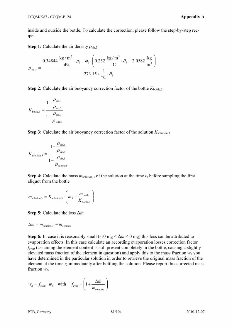
CCQM-K87 / CCQM-P124 Appendix A
PTB, Germany 81/104 2010-12-07
inside and outside the bottle. To calculate the correction, please follow the step-by-step rec-ipe:
Step 1: Calculate the air density ρair,3
3
33
3
33
3
3,air
C115.273
mkg0582.2
Cm/kg252.0
hPam/kg34844.0
ϑ
ϑϕρ
⋅°
+
⎟⎟⎠
⎞⎜⎜⎝
⎛−⋅
°⋅−⋅
=p
Step 2: Calculate the air buoyancy correction factor of the bottle Kbottle,3
bottle
3,air
cal,3
3,air
bottle,3
1
1
ρρρρ
−
−
=K
Step 3: Calculate the air buoyancy correction factor of the solution Ksolution,3
solution
3,air
cal,3
3,air
solution,3
1
1
ρρρρ
−
−
=K
Step 4: Calculate the mass msolution,3 of the solution at the time t3 before sampling the first aliquot from the bottle
⎟⎟⎠
⎞⎜⎜⎝
⎛−⋅=
bottle,3
bottle3solution,3solution,3 K
mmKm
Step 5: Calculate the loss ∆m
solutionsolution,3 mmm −=Δ
Step 6: In case it is reasonably small (-10 mg < ∆m < 0 mg) this loss can be attributed to evaporation effects. In this case calculate an according evaporation losses correction factor fevap (assuming the element content is still present completely in the bottle, causing a slightly elevated mass fraction of the element in question) and apply this to the mass fraction w3 you have determined in the particular solution in order to retrieve the original mass fraction of the element at the time t2 immediately after bottling the solution. Please report this corrected mass fraction w2.
⎟⎟⎠
⎞⎜⎜⎝
⎛ Δ+=⋅=
solutionevap3evap2 1with
mmfwfw
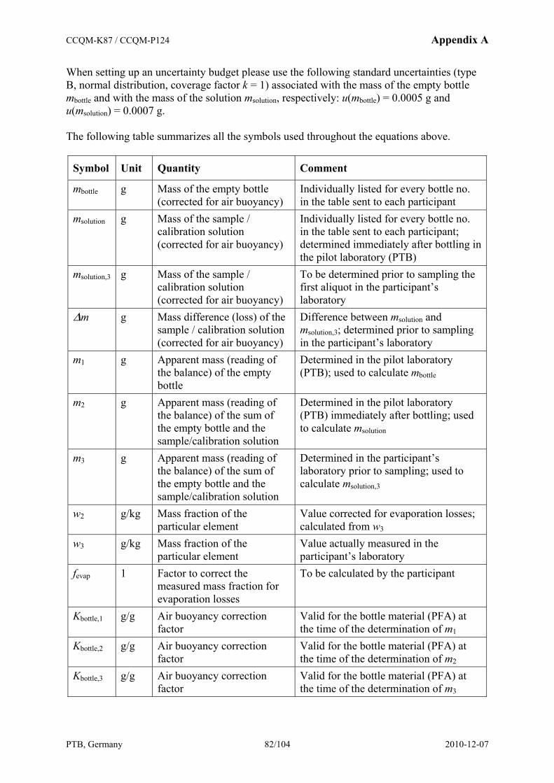
CCQM-K87 / CCQM-P124 Appendix A
PTB, Germany 82/104 2010-12-07
When setting up an uncertainty budget please use the following standard uncertainties (type B, normal distribution, coverage factor k = 1) associated with the mass of the empty bottle mbottle and with the mass of the solution msolution, respectively: u(mbottle) = 0.0005 g and u(msolution) = 0.0007 g. The following table summarizes all the symbols used throughout the equations above.
Symbol Unit Quantity Comment
mbottle g Mass of the empty bottle (corrected for air buoyancy)
Individually listed for every bottle no. in the table sent to each participant
msolution g Mass of the sample / calibration solution (corrected for air buoyancy)
Individually listed for every bottle no. in the table sent to each participant; determined immediately after bottling in the pilot laboratory (PTB)
msolution,3 g Mass of the sample / calibration solution (corrected for air buoyancy)
To be determined prior to sampling the first aliquot in the participant’s laboratory
∆m g Mass difference (loss) of the sample / calibration solution (corrected for air buoyancy)
Difference between msolution and msolution,3; determined prior to sampling in the participant’s laboratory
m1 g Apparent mass (reading of the balance) of the empty bottle
Determined in the pilot laboratory (PTB); used to calculate mbottle
m2 g Apparent mass (reading of the balance) of the sum of the empty bottle and the sample/calibration solution
Determined in the pilot laboratory (PTB) immediately after bottling; used to calculate msolution
m3 g Apparent mass (reading of the balance) of the sum of the empty bottle and the sample/calibration solution
Determined in the participant’s laboratory prior to sampling; used to calculate msolution,3
w2 g/kg Mass fraction of the particular element
Value corrected for evaporation losses; calculated from w3
w3 g/kg Mass fraction of the particular element
Value actually measured in the participant’s laboratory
fevap 1 Factor to correct the measured mass fraction for evaporation losses
To be calculated by the participant
Kbottle,1 g/g Air buoyancy correction factor
Valid for the bottle material (PFA) at the time of the determination of m1
Kbottle,2 g/g Air buoyancy correction factor
Valid for the bottle material (PFA) at the time of the determination of m2
Kbottle,3 g/g Air buoyancy correction factor
Valid for the bottle material (PFA) at the time of the determination of m3
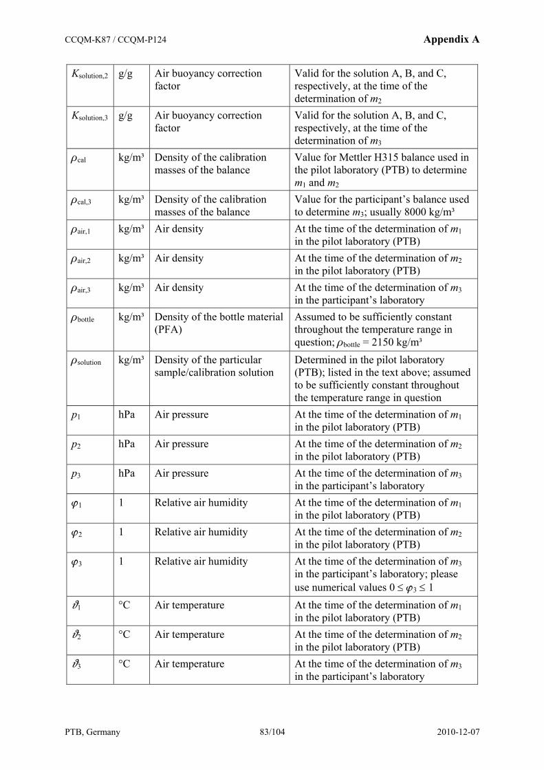
CCQM-K87 / CCQM-P124 Appendix A
PTB, Germany 83/104 2010-12-07
Ksolution,2 g/g Air buoyancy correction factor
Valid for the solution A, B, and C, respectively, at the time of the determination of m2
Ksolution,3 g/g Air buoyancy correction factor
Valid for the solution A, B, and C, respectively, at the time of the determination of m3
ρcal kg/m³ Density of the calibration masses of the balance
Value for Mettler H315 balance used in the pilot laboratory (PTB) to determine m1 and m2
ρcal,3 kg/m³ Density of the calibration masses of the balance
Value for the participant’s balance used to determine m3; usually 8000 kg/m³
ρair,1 kg/m³ Air density At the time of the determination of m1 in the pilot laboratory (PTB)
ρair,2 kg/m³ Air density At the time of the determination of m2 in the pilot laboratory (PTB)
ρair,3 kg/m³ Air density At the time of the determination of m3 in the participant’s laboratory
ρbottle kg/m³ Density of the bottle material (PFA)
Assumed to be sufficiently constant throughout the temperature range in question; ρbottle = 2150 kg/m³
ρsolution kg/m³ Density of the particular sample/calibration solution
Determined in the pilot laboratory (PTB); listed in the text above; assumed to be sufficiently constant throughout the temperature range in question
p1 hPa Air pressure At the time of the determination of m1 in the pilot laboratory (PTB)
p2 hPa Air pressure At the time of the determination of m2 in the pilot laboratory (PTB)
p3 hPa Air pressure At the time of the determination of m3 in the participant’s laboratory
ϕ1 1 Relative air humidity At the time of the determination of m1 in the pilot laboratory (PTB)
ϕ2 1 Relative air humidity At the time of the determination of m2 in the pilot laboratory (PTB)
ϕ3 1 Relative air humidity At the time of the determination of m3 in the participant’s laboratory; please use numerical values 0 ≤ ϕ3 ≤ 1
ϑ1 °C Air temperature At the time of the determination of m1 in the pilot laboratory (PTB)
ϑ2 °C Air temperature At the time of the determination of m2 in the pilot laboratory (PTB)
ϑ3 °C Air temperature At the time of the determination of m3 in the participant’s laboratory

CCQM-K87 / CCQM-P124 Appendix A
PTB, Germany 84/104 2010-12-07
7. References [1] Evaluation of measurement data – Guide to the expression of uncertainty in measurement,
JCGM 100:2008. [2] Frank Spieweck, Horst Bettin, Methoden zur Bestimmung der Dichte von Festkörpern und
Flüssigkeiten, PTB Bericht W-46, ISBN 3-89429-132-X, Braunschweig, 1998. [3] Roland Nater, Arthur Reichmuth, Roman Schwartz, Michael Borys, Panagiotis Zervos,
Dictionary of Weighing Terms, A Guide to the Terminology of Weighing, Springer, ISBN 978-3-642-02013-1, Berlin, 2009.
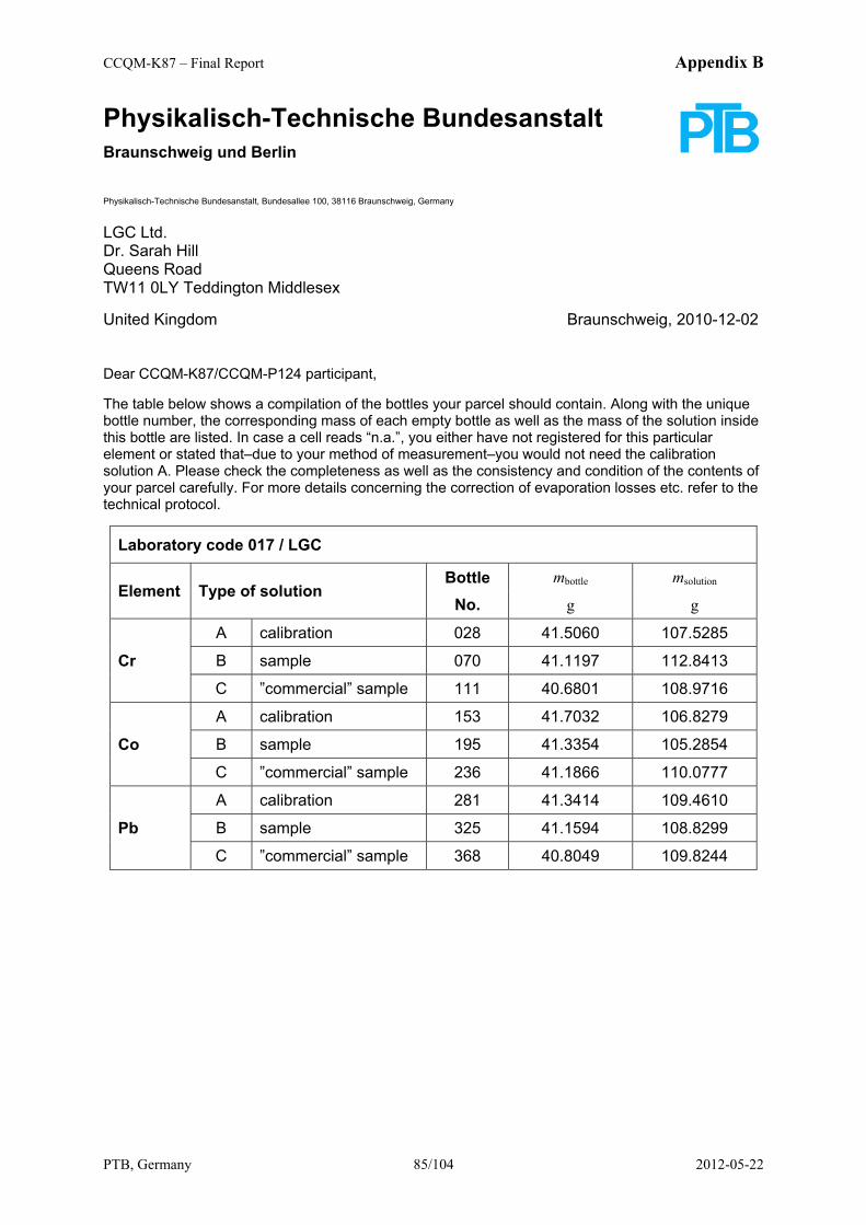
CCQM-K87 – Final Report Appendix B
PTB, Germany 85/104 2012-05-22
Physikalisch-Technische Bundesanstalt
Braunschweig und Berlin Physikalisch-Technische Bundesanstalt, Bundesallee 100, 38116 Braunschweig, Germany
LGC Ltd. Dr. Sarah Hill Queens Road TW11 0LY Teddington Middlesex United Kingdom Braunschweig, 2010-12-02 Dear CCQM-K87/CCQM-P124 participant, The table below shows a compilation of the bottles your parcel should contain. Along with the unique bottle number, the corresponding mass of each empty bottle as well as the mass of the solution inside this bottle are listed. In case a cell reads “n.a.”, you either have not registered for this particular element or stated that–due to your method of measurement–you would not need the calibration solution A. Please check the completeness as well as the consistency and condition of the contents of your parcel carefully. For more details concerning the correction of evaporation losses etc. refer to the technical protocol.
Laboratory code 017 / LGC
Element Type of solution Bottle
No. mbottle msolution
g g
Cr
A calibration 028 41.5060 107.5285
B sample 070 41.1197 112.8413
C ”commercial” sample 111 40.6801 108.9716
Co
A calibration 153 41.7032 106.8279
B sample 195 41.3354 105.2854
C ”commercial” sample 236 41.1866 110.0777
Pb
A calibration 281 41.3414 109.4610
B sample 325 41.1594 108.8299
C ”commercial” sample 368 40.8049 109.8244
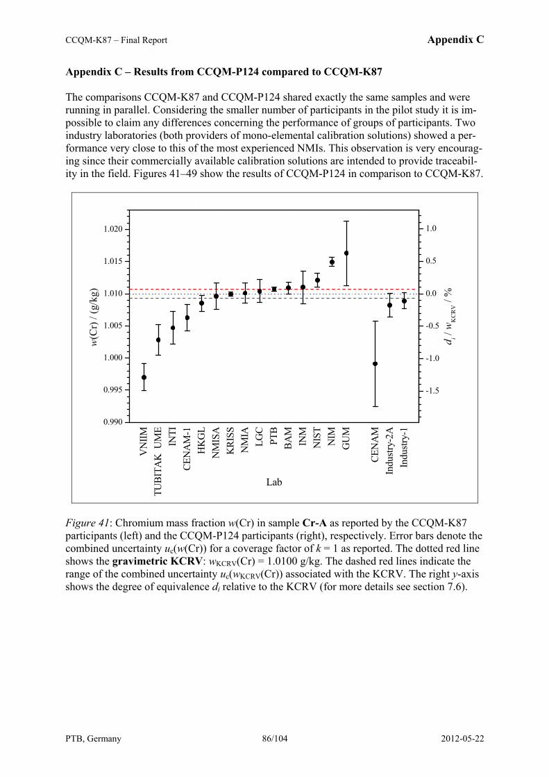
CCQM-K87 – Final Report Appendix C
PTB, Germany 86/104 2012-05-22
Appendix C – Results from CCQM-P124 compared to CCQM-K87 The comparisons CCQM-K87 and CCQM-P124 shared exactly the same samples and were running in parallel. Considering the smaller number of participants in the pilot study it is im-possible to claim any differences concerning the performance of groups of participants. Two industry laboratories (both providers of mono-elemental calibration solutions) showed a per-formance very close to this of the most experienced NMIs. This observation is very encourag-ing since their commercially available calibration solutions are intended to provide traceabil-ity in the field. Figures 41–49 show the results of CCQM-P124 in comparison to CCQM-K87.
VN
IIMTU
BITA
K U
ME
INTI
CEN
AM
-1H
KG
LN
MIS
AK
RISS
NM
IALG
CPT
BBA
MIN
MN
IST
NIM
GU
M
CEN
AM
Indu
stry-
2AIn
dustr
y-1
0.990
0.995
1.000
1.005
1.010
1.015
1.020
w(C
r) /
(g/k
g)
Lab
-1.5
-1.0
-0.5
0.0
0.5
1.0
di /
wK
CR
V /
%
Figure 41: Chromium mass fraction w(Cr) in sample Cr-A as reported by the CCQM-K87 participants (left) and the CCQM-P124 participants (right), respectively. Error bars denote the combined uncertainty uc(w(Cr)) for a coverage factor of k = 1 as reported. The dotted red line shows the gravimetric KCRV: wKCRV(Cr) = 1.0100 g/kg. The dashed red lines indicate the range of the combined uncertainty uc(wKCRV(Cr)) associated with the KCRV. The right y-axis shows the degree of equivalence di relative to the KCRV (for more details see section 7.6).
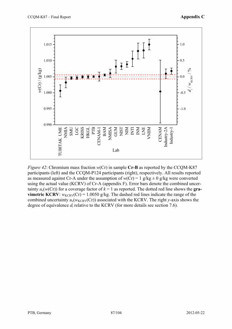
CCQM-K87 – Final Report Appendix C
PTB, Germany 87/104 2012-05-22
TUBI
TAK
UM
EN
MIA
SMU
LGC
KRI
SSH
KG
LPT
BCE
NA
M-1
BAM
NM
ISA
GU
MN
IST
NIM
INTI
INM
LNE
VN
IIM
CEN
AM
Indu
stry-
2AIn
dustr
y-1
0.990
0.995
1.000
1.005
1.010
1.015w
(Cr)
/ (g
/kg)
Lab
-1.0
-0.5
0.0
0.5
1.0
di /
wK
CR
V /
%
Figure 42: Chromium mass fraction w(Cr) in sample Cr-B as reported by the CCQM-K87 participants (left) and the CCQM-P124 participants (right), respectively. All results reported as measured against Cr-A under the assumption of w(Cr) = 1 g/kg ± 0 g/kg were converted using the actual value (KCRV) of Cr-A (appendix F). Error bars denote the combined uncer-tainty uc(w(Cr)) for a coverage factor of k = 1 as reported. The dotted red line shows the gra-vimetric KCRV: wKCRV(Cr) = 1.0050 g/kg. The dashed red lines indicate the range of the combined uncertainty uc(wKCRV(Cr)) associated with the KCRV. The right y-axis shows the degree of equivalence di relative to the KCRV (for more details see section 7.6).
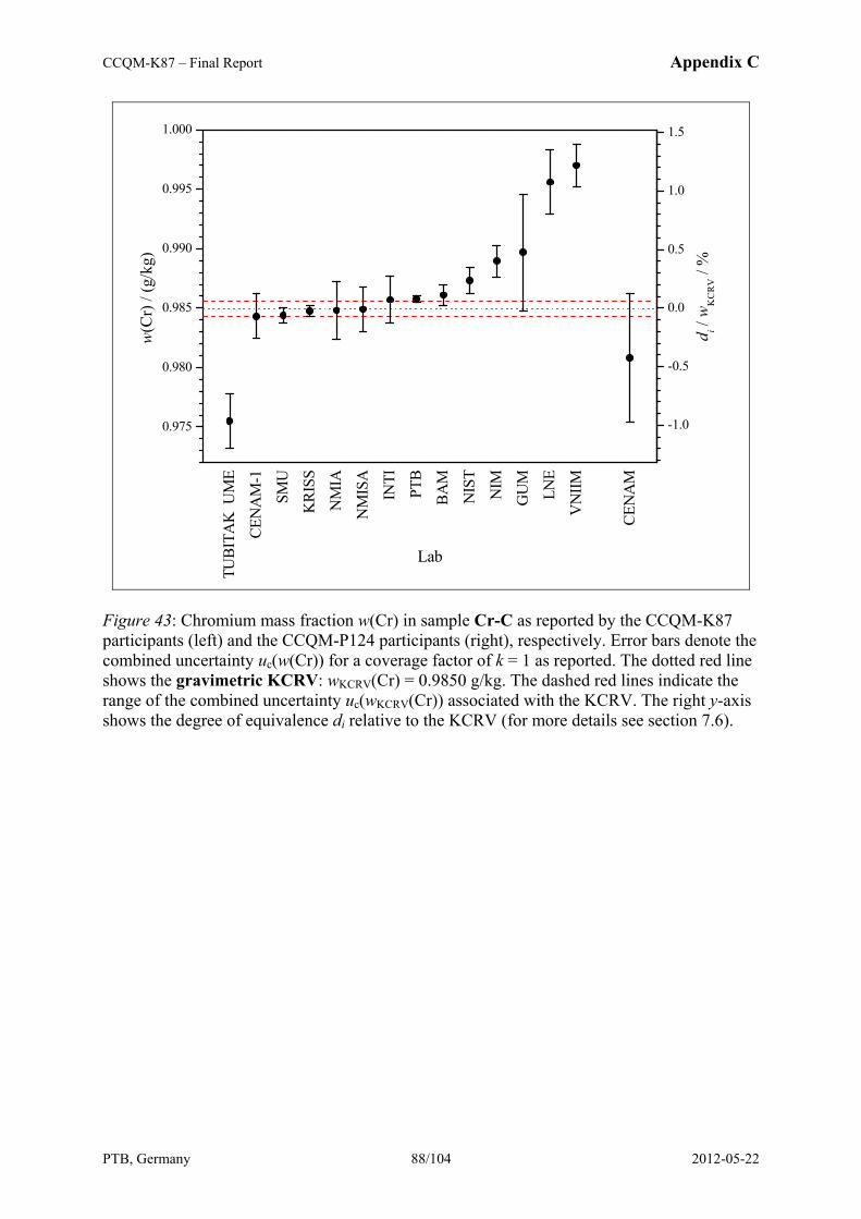
CCQM-K87 – Final Report Appendix C
PTB, Germany 88/104 2012-05-22
TUBI
TAK
UM
E
CEN
AM
-1
SMU
KRI
SS
NM
IA
NM
ISA
INTI
PTB
BAM
NIS
T
NIM
GU
M
LNE
VN
IIM
CEN
AM
0.975
0.980
0.985
0.990
0.995
1.000w
(Cr)
/ (g
/kg)
Lab
-1.0
-0.5
0.0
0.5
1.0
1.5
di /
wK
CR
V /
%
Figure 43: Chromium mass fraction w(Cr) in sample Cr-C as reported by the CCQM-K87 participants (left) and the CCQM-P124 participants (right), respectively. Error bars denote the combined uncertainty uc(w(Cr)) for a coverage factor of k = 1 as reported. The dotted red line shows the gravimetric KCRV: wKCRV(Cr) = 0.9850 g/kg. The dashed red lines indicate the range of the combined uncertainty uc(wKCRV(Cr)) associated with the KCRV. The right y-axis shows the degree of equivalence di relative to the KCRV (for more details see section 7.6).
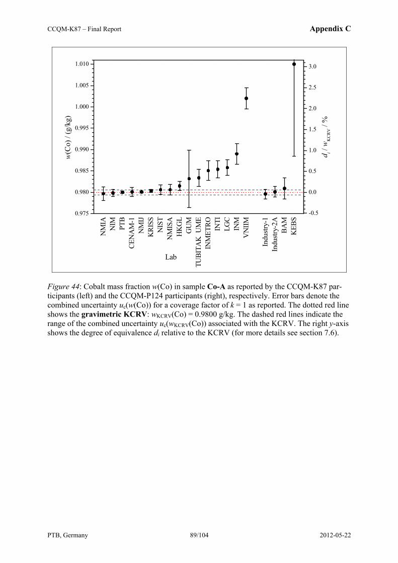
CCQM-K87 – Final Report Appendix C
PTB, Germany 89/104 2012-05-22
NM
IAN
IM PTB
CEN
AM
-1N
MIJ
KRI
SSN
IST
NM
ISA
HK
GL
GU
MTU
BITA
K U
ME
INM
ETRO INTI
LGC
INM
VN
IIM
Indu
stry-
1In
dustr
y-2A
BAM
KEB
S
0.975
0.980
0.985
0.990
0.995
1.000
1.005
1.010w
(Co)
/ (g
/kg)
Lab
-0.5
0.0
0.5
1.0
1.5
2.0
2.5
3.0
di /
wK
CR
V /
%
Figure 44: Cobalt mass fraction w(Co) in sample Co-A as reported by the CCQM-K87 par-ticipants (left) and the CCQM-P124 participants (right), respectively. Error bars denote the combined uncertainty uc(w(Co)) for a coverage factor of k = 1 as reported. The dotted red line shows the gravimetric KCRV: wKCRV(Co) = 0.9800 g/kg. The dashed red lines indicate the range of the combined uncertainty uc(wKCRV(Co)) associated with the KCRV. The right y-axis shows the degree of equivalence di relative to the KCRV (for more details see section 7.6).
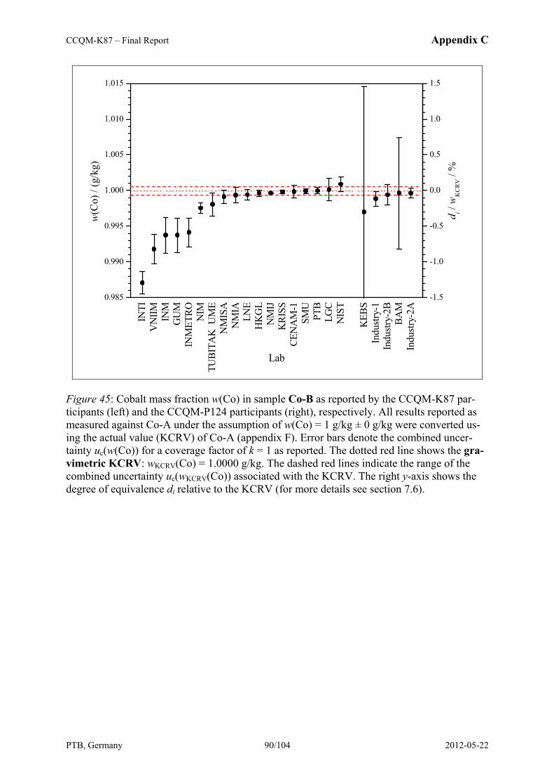
CCQM-K87 – Final Report Appendix C
PTB, Germany 90/104 2012-05-22
INTI
VN
IIM INM
GU
MIN
MET
RO NIM
TUBI
TAK
UM
EN
MIS
AN
MIA
LNE
HK
GL
NM
IJK
RISS
CEN
AM
-1SM
UPT
BLG
CN
IST
KEB
SIn
dustr
y-1
Indu
stry-
2BBA
MIn
dustr
y-2A
0.985
0.990
0.995
1.000
1.005
1.010
1.015w
(Co)
/ (g
/kg)
Lab
-1.5
-1.0
-0.5
0.0
0.5
1.0
1.5
di /
wK
CR
V /
%
Figure 45: Cobalt mass fraction w(Co) in sample Co-B as reported by the CCQM-K87 par-ticipants (left) and the CCQM-P124 participants (right), respectively. All results reported as measured against Co-A under the assumption of w(Co) = 1 g/kg ± 0 g/kg were converted us-ing the actual value (KCRV) of Co-A (appendix F). Error bars denote the combined uncer-tainty uc(w(Co)) for a coverage factor of k = 1 as reported. The dotted red line shows the gra-vimetric KCRV: wKCRV(Co) = 1.0000 g/kg. The dashed red lines indicate the range of the combined uncertainty uc(wKCRV(Co)) associated with the KCRV. The right y-axis shows the degree of equivalence di relative to the KCRV (for more details see section 7.6).
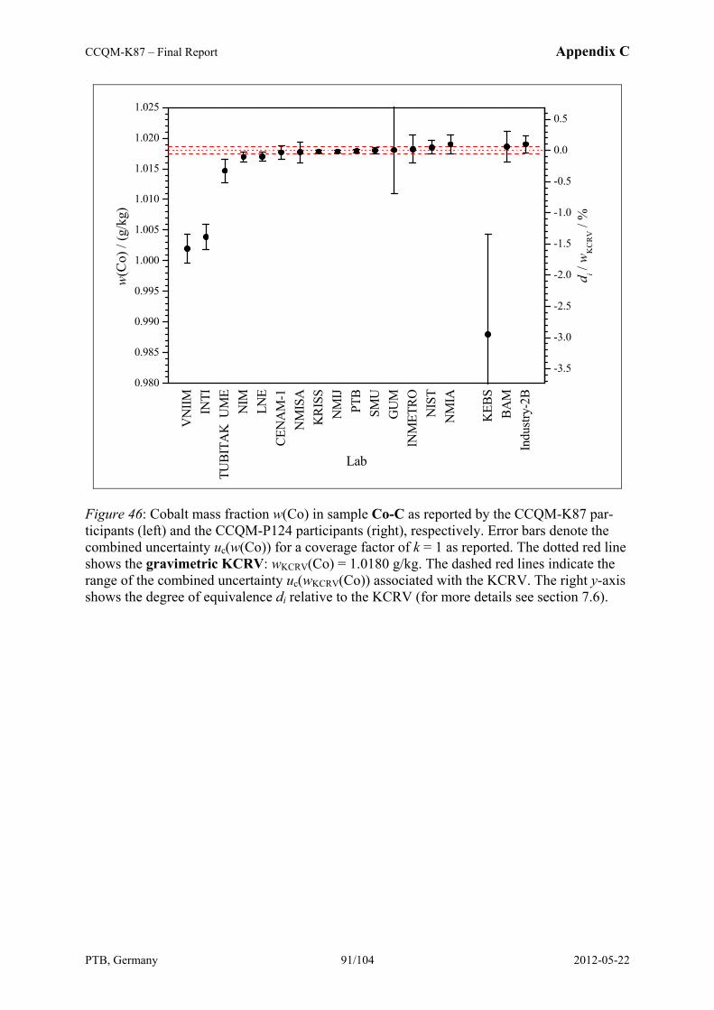
CCQM-K87 – Final Report Appendix C
PTB, Germany 91/104 2012-05-22
VN
IIM INTI
TUBI
TAK
UM
EN
IMLN
ECE
NA
M-1
NM
ISA
KRI
SSN
MIJ
PTB
SMU
GU
MIN
MET
RON
IST
NM
IA
KEB
SBA
MIn
dustr
y-2B
0.980
0.985
0.990
0.995
1.000
1.005
1.010
1.015
1.020
1.025w
(Co)
/ (g
/kg)
Lab
-3.5
-3.0
-2.5
-2.0
-1.5
-1.0
-0.5
0.0
0.5
di /
wK
CR
V /
%
Figure 46: Cobalt mass fraction w(Co) in sample Co-C as reported by the CCQM-K87 par-ticipants (left) and the CCQM-P124 participants (right), respectively. Error bars denote the combined uncertainty uc(w(Co)) for a coverage factor of k = 1 as reported. The dotted red line shows the gravimetric KCRV: wKCRV(Co) = 1.0180 g/kg. The dashed red lines indicate the range of the combined uncertainty uc(wKCRV(Co)) associated with the KCRV. The right y-axis shows the degree of equivalence di relative to the KCRV (for more details see section 7.6).

CCQM-K87 – Final Report Appendix C
PTB, Germany 92/104 2012-05-22
BAM
NM
IJPT
BLG
CN
IMK
RISS
CEN
AM
-1H
KG
LN
IST
NM
IAN
MIS
AIN
MTU
BITA
K U
ME
VN
IIM INTI
GU
M
KEB
SIn
dustr
y-1
Indu
stry-
2ABA
MN
IMT
0.950
0.955
0.960
0.965
0.970
0.975
0.980
0.985
0.990
0.995
1.000
1.005
1.010
1.03
59
w(P
b) /
(g/k
g)
Lab
1.08
77
-3.0
-2.5
-2.0
-1.5
-1.0
-0.5
0.0
0.5
1.0
1.5
2.0
2.5
3.0
di /
wK
CR
V /
%
Figure 47: Lead mass fraction w(Pb) in sample Pb-A as reported by the CCQM-K87 partici-pants (left) and the CCQM-P124 participants (right), respectively. Results reported in terms of amount contents n/m converted in mass fractions w applying a molar mass of M(Pb) = (207.17782 ± 0.00011) g/mol (k = 2), refer to section 2.3 for details. Error bars denote the combined uncertainty uc(w(Pb)) for a coverage factor of k = 1 as reported. The dotted red line shows the gravimetric KCRV: wKCRV(Pb) = 0.9800 g/kg. The dashed red lines indicate the range of the combined uncertainty uc(wKCRV(Pb)) associated with the KCRV. The right y-axis shows the degree of equivalence di relative to the KCRV (for more details see section 7.6).
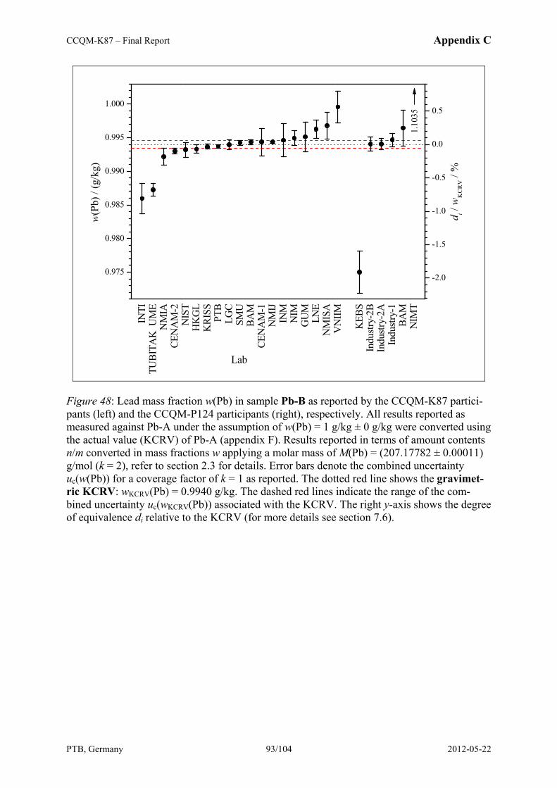
CCQM-K87 – Final Report Appendix C
PTB, Germany 93/104 2012-05-22
INTI
TUBI
TAK
UM
EN
MIA
CEN
AM
-2N
IST
HK
GL
KRI
SSPT
BLG
CSM
UBA
MCE
NA
M-1
NM
IJIN
MN
IMG
UM
LNE
NM
ISA
VN
IIM
KEB
SIn
dustr
y-2B
Indu
stry-
2AIn
dustr
y-1
BAM
NIM
T
0.975
0.980
0.985
0.990
0.995
1.000w
(Pb)
/ (g
/kg)
Lab
1.10
35
-2.0
-1.5
-1.0
-0.5
0.0
0.5
di /
wK
CR
V /
%
Figure 48: Lead mass fraction w(Pb) in sample Pb-B as reported by the CCQM-K87 partici-pants (left) and the CCQM-P124 participants (right), respectively. All results reported as measured against Pb-A under the assumption of w(Pb) = 1 g/kg ± 0 g/kg were converted using the actual value (KCRV) of Pb-A (appendix F). Results reported in terms of amount contents n/m converted in mass fractions w applying a molar mass of M(Pb) = (207.17782 ± 0.00011) g/mol (k = 2), refer to section 2.3 for details. Error bars denote the combined uncertainty uc(w(Pb)) for a coverage factor of k = 1 as reported. The dotted red line shows the gravimet-ric KCRV: wKCRV(Pb) = 0.9940 g/kg. The dashed red lines indicate the range of the com-bined uncertainty uc(wKCRV(Pb)) associated with the KCRV. The right y-axis shows the degree of equivalence di relative to the KCRV (for more details see section 7.6).
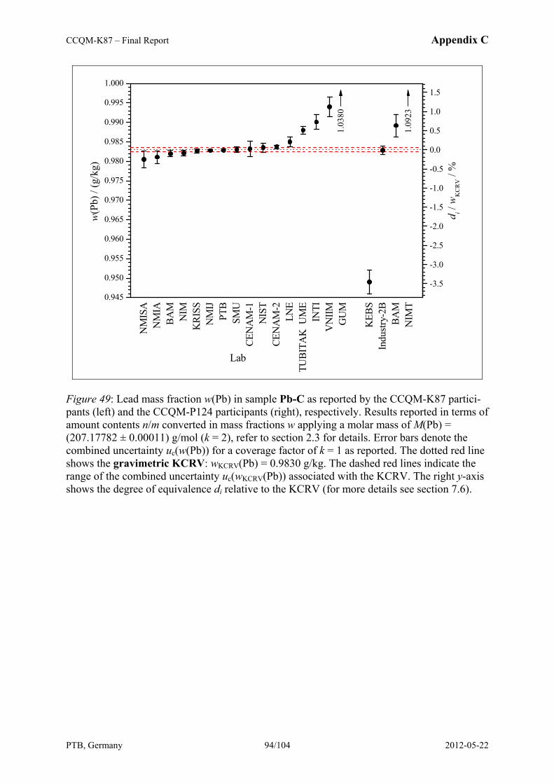
CCQM-K87 – Final Report Appendix C
PTB, Germany 94/104 2012-05-22
NM
ISA
NM
IABA
MN
IMK
RISS
NM
IJPT
BSM
UCE
NA
M-1
NIS
TCE
NA
M-2
LNE
TUBI
TAK
UM
EIN
TIV
NIIM
GU
M
KEB
SIn
dustr
y-2B
BAM
NIM
T
0.945
0.950
0.955
0.960
0.965
0.970
0.975
0.980
0.985
0.990
0.995
1.000w
(Pb)
/ (g
/kg)
Lab
-3.5
-3.0
-2.5
-2.0
-1.5
-1.0
-0.5
0.0
0.5
1.0
1.5
1.03
80
di /
wK
CR
V /
%
1.09
23
Figure 49: Lead mass fraction w(Pb) in sample Pb-C as reported by the CCQM-K87 partici-pants (left) and the CCQM-P124 participants (right), respectively. Results reported in terms of amount contents n/m converted in mass fractions w applying a molar mass of M(Pb) = (207.17782 ± 0.00011) g/mol (k = 2), refer to section 2.3 for details. Error bars denote the combined uncertainty uc(w(Pb)) for a coverage factor of k = 1 as reported. The dotted red line shows the gravimetric KCRV: wKCRV(Pb) = 0.9830 g/kg. The dashed red lines indicate the range of the combined uncertainty uc(wKCRV(Pb)) associated with the KCRV. The right y-axis shows the degree of equivalence di relative to the KCRV (for more details see section 7.6).
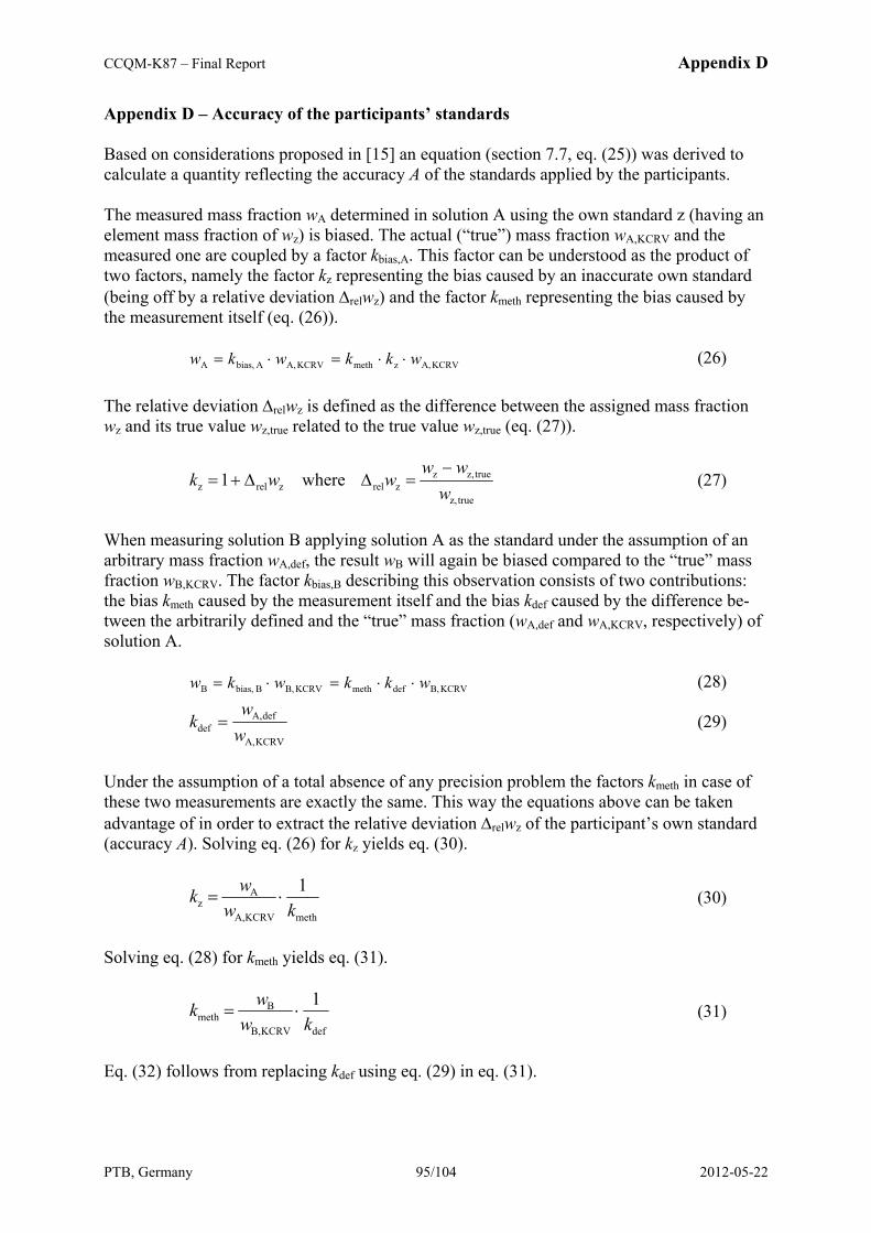
CCQM-K87 – Final Report Appendix D
PTB, Germany 95/104 2012-05-22
Appendix D – Accuracy of the participants’ standards Based on considerations proposed in [15] an equation (section 7.7, eq. (25)) was derived to calculate a quantity reflecting the accuracy A of the standards applied by the participants. The measured mass fraction wA determined in solution A using the own standard z (having an element mass fraction of wz) is biased. The actual (“true”) mass fraction wA,KCRV and the measured one are coupled by a factor kbias,A. This factor can be understood as the product of two factors, namely the factor kz representing the bias caused by an inaccurate own standard (being off by a relative deviation Δrelwz) and the factor kmeth representing the bias caused by the measurement itself (eq. (26)). KCRVA,zmethKCRVA,Abias,A wkkwkw ⋅⋅=⋅= (26) The relative deviation Δrelwz is defined as the difference between the assigned mass fraction wz and its true value wz,true related to the true value wz,true (eq. (27)).
truez,
truez,zzrelzrelz where1
www
wwk−
=ΔΔ+= (27)
When measuring solution B applying solution A as the standard under the assumption of an arbitrary mass fraction wA,def, the result wB will again be biased compared to the “true” mass fraction wB,KCRV. The factor kbias,B describing this observation consists of two contributions: the bias kmeth caused by the measurement itself and the bias kdef caused by the difference be-tween the arbitrarily defined and the “true” mass fraction (wA,def and wA,KCRV, respectively) of solution A. KCRVB,defmethKCRVB,Bbias,B wkkwkw ⋅⋅=⋅= (28)
KCRVA,
defA,def w
wk = (29)
Under the assumption of a total absence of any precision problem the factors kmeth in case of these two measurements are exactly the same. This way the equations above can be taken advantage of in order to extract the relative deviation Δrelwz of the participant’s own standard (accuracy A). Solving eq. (26) for kz yields eq. (30).
methKCRVA,
Az
1kw
wk ⋅= (30)
Solving eq. (28) for kmeth yields eq. (31).
defKCRVB,
Bmeth
1kw
wk ⋅= (31)
Eq. (32) follows from replacing kdef using eq. (29) in eq. (31).
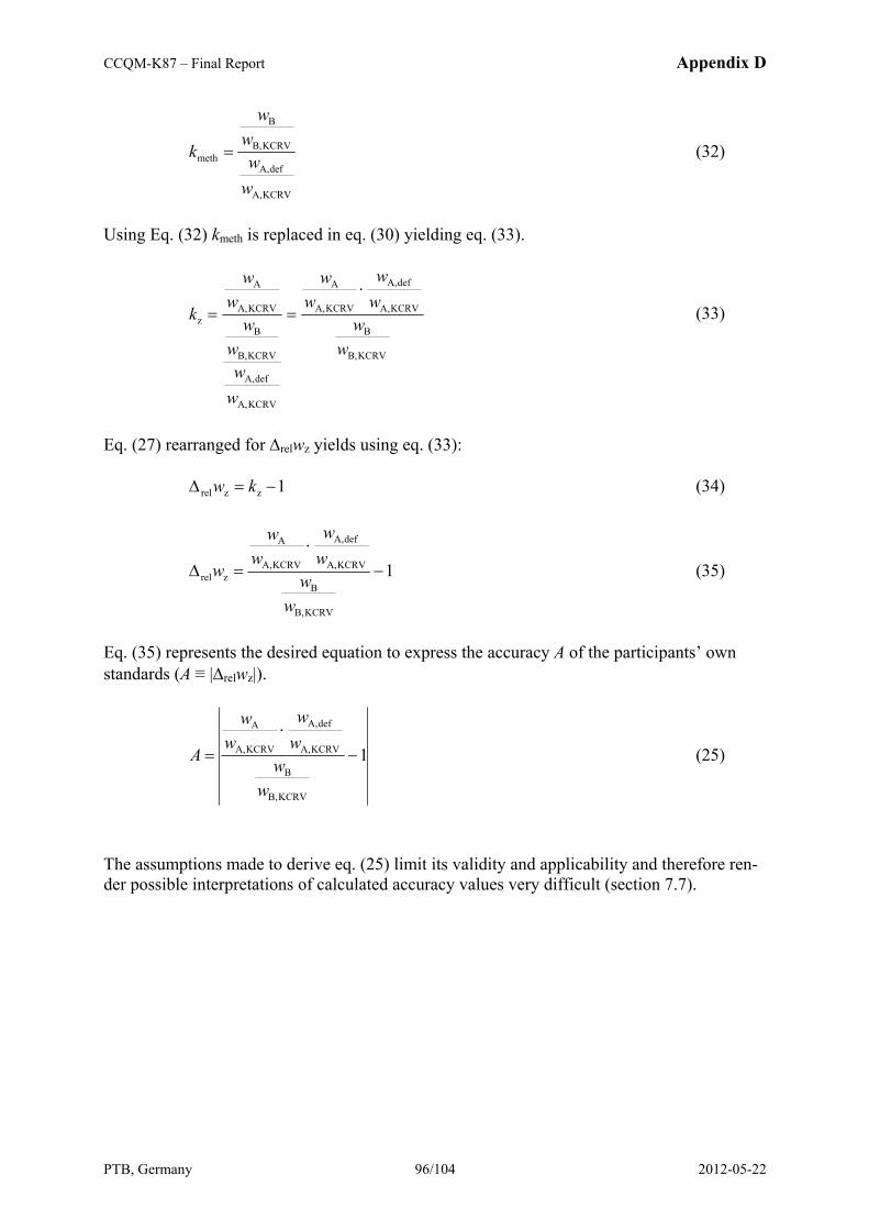
CCQM-K87 – Final Report Appendix D
PTB, Germany 96/104 2012-05-22
KCRVA,
defA,
KCRVB,
B
meth
ww
ww
k = (32)
Using Eq. (32) kmeth is replaced in eq. (30) yielding eq. (33).
KCRVB,
B
KCRVA,
defA,
KCRVA,
A
KCRVA,
defA,
KCRVB,
B
KCRVA,
A
z
ww
ww
ww
ww
ww
ww
k⋅
== (33)
Eq. (27) rearranged for Δrelwz yields using eq. (33): 1zzrel −=Δ kw (34)
1
KCRVB,
B
KCRVA,
defA,
KCRVA,
A
zrel −⋅
=Δ
ww
ww
ww
w (35)
Eq. (35) represents the desired equation to express the accuracy A of the participants’ own standards (A ≡ |Δrelwz|).
1
KCRVB,
B
KCRVA,
defA,
KCRVA,
A
−⋅
=
ww
ww
ww
A (25)
The assumptions made to derive eq. (25) limit its validity and applicability and therefore ren-der possible interpretations of calculated accuracy values very difficult (section 7.7).
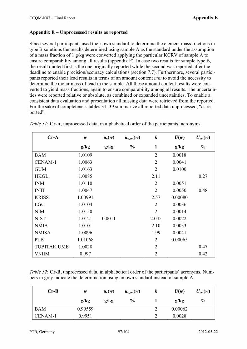
CCQM-K87 – Final Report Appendix E
PTB, Germany 97/104 2012-05-22
Appendix E – Unprocessed results as reported Since several participants used their own standard to determine the element mass fractions in type B solutions the results determined using sample A as the standard under the assumption of a mass fraction of 1 g/kg were converted applying the particular KCRV of sample A to ensure comparability among all results (appendix F). In case two results for sample type B, the result quoted first is the one originally reported while the second was reported after the deadline to enable precision/accuracy calculations (section 7.7). Furthermore, several partici-pants reported their lead results in terms of an amount content n/m to avoid the necessity to determine the molar mass of lead in the sample. All these amount content results were con-verted to yield mass fractions, again to ensure comparability among all results. The uncertain-ties were reported relative or absolute, as combined or expanded uncertainties. To enable a consistent data evaluation and presentation all missing data were retrieved from the reported. For the sake of completeness tables 31–39 summarize all reported data unprocessed, “as re-ported”. Table 31: Cr-A, unprocessed data, in alphabetical order of the participants’ acronyms.
Cr-A w uc(w) uc,rel(w) k U(w) Urel(w)
g/kg g/kg % 1 g/kg %
BAM 1.0109 2 0.0018 CENAM-1 1.0063 2 0.0041 GUM 1.0163 2 0.0100 HKGL 1.0085 2.11 0.27 INM 1.0110 2 0.0051 INTI 1.0047 2 0.0050 0.48 KRISS 1.00991 2.57 0.00080 LGC 1.0104 2 0.0036 NIM 1.0150 2 0.0014 NIST 1.0121 0.0011 2.045 0.0022 NMIA 1.0101 2.10 0.0033 NMISA 1.0096 1.99 0.0041 PTB 1.01068 2 0.00065 TUBITAK UME 1.0028 2 0.47 VNIIM 0.997 2 0.42
Table 32: Cr-B, unprocessed data, in alphabetical order of the participants’ acronyms. Num-bers in grey indicate the determination using an own standard instead of sample A.
Cr-B w uc(w) uc,rel(w) k U(w) Urel(w)
g/kg g/kg % 1 g/kg %
BAM 0.99559 2 0.00062 CENAM-1 0.9951 2 0.0028
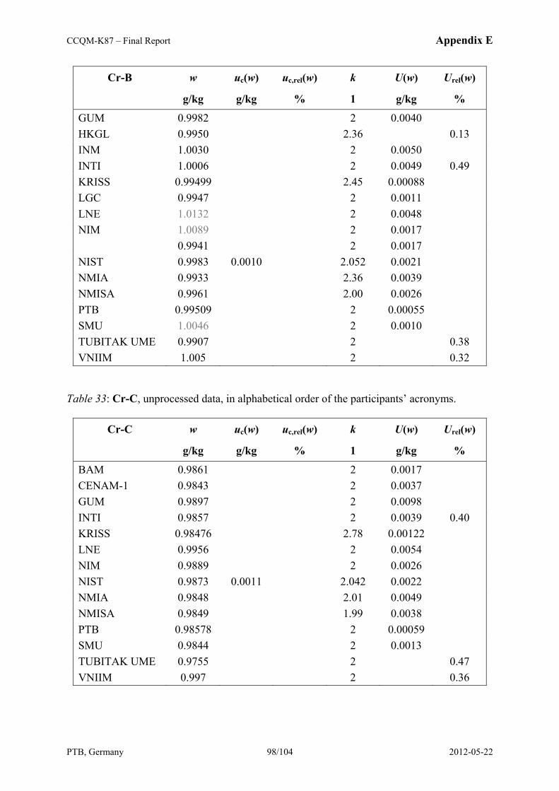
CCQM-K87 – Final Report Appendix E
PTB, Germany 98/104 2012-05-22
Cr-B w uc(w) uc,rel(w) k U(w) Urel(w)
g/kg g/kg % 1 g/kg %
GUM 0.9982 2 0.0040 HKGL 0.9950 2.36 0.13 INM 1.0030 2 0.0050 INTI 1.0006 2 0.0049 0.49 KRISS 0.99499 2.45 0.00088 LGC 0.9947 2 0.0011 LNE 1.0132 2 0.0048 NIM 1.0089 2 0.0017 0.9941 2 0.0017 NIST 0.9983 0.0010 2.052 0.0021 NMIA 0.9933 2.36 0.0039 NMISA 0.9961 2.00 0.0026 PTB 0.99509 2 0.00055 SMU 1.0046 2 0.0010 TUBITAK UME 0.9907 2 0.38 VNIIM 1.005 2 0.32
Table 33: Cr-C, unprocessed data, in alphabetical order of the participants’ acronyms.
Cr-C w uc(w) uc,rel(w) k U(w) Urel(w)
g/kg g/kg % 1 g/kg %
BAM 0.9861 2 0.0017 CENAM-1 0.9843 2 0.0037 GUM 0.9897 2 0.0098 INTI 0.9857 2 0.0039 0.40 KRISS 0.98476 2.78 0.00122 LNE 0.9956 2 0.0054 NIM 0.9889 2 0.0026 NIST 0.9873 0.0011 2.042 0.0022 NMIA 0.9848 2.01 0.0049 NMISA 0.9849 1.99 0.0038 PTB 0.98578 2 0.00059 SMU 0.9844 2 0.0013 TUBITAK UME 0.9755 2 0.47 VNIIM 0.997 2 0.36
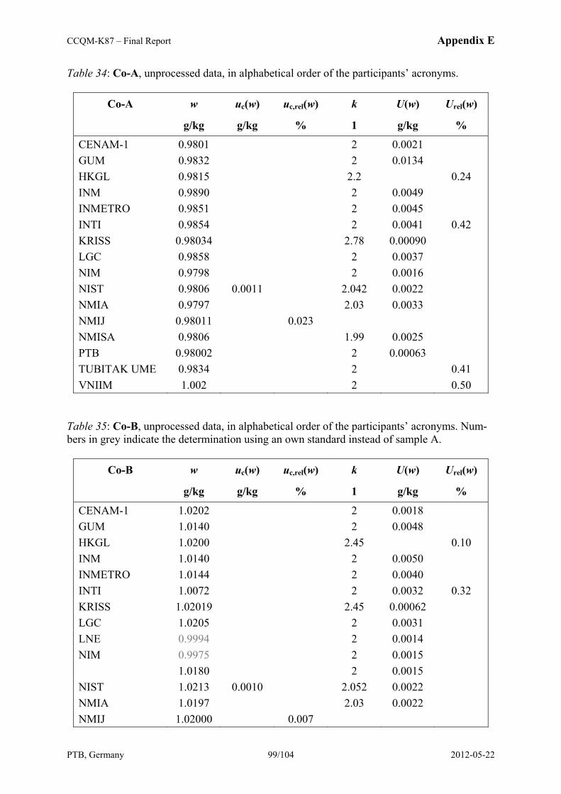
CCQM-K87 – Final Report Appendix E
PTB, Germany 99/104 2012-05-22
Table 34: Co-A, unprocessed data, in alphabetical order of the participants’ acronyms.
Co-A w uc(w) uc,rel(w) k U(w) Urel(w)
g/kg g/kg % 1 g/kg %
CENAM-1 0.9801 2 0.0021 GUM 0.9832 2 0.0134 HKGL 0.9815 2.2 0.24 INM 0.9890 2 0.0049 INMETRO 0.9851 2 0.0045 INTI 0.9854 2 0.0041 0.42 KRISS 0.98034 2.78 0.00090 LGC 0.9858 2 0.0037 NIM 0.9798 2 0.0016 NIST 0.9806 0.0011 2.042 0.0022 NMIA 0.9797 2.03 0.0033 NMIJ 0.98011 0.023 NMISA 0.9806 1.99 0.0025 PTB 0.98002 2 0.00063 TUBITAK UME 0.9834 2 0.41 VNIIM 1.002 2 0.50
Table 35: Co-B, unprocessed data, in alphabetical order of the participants’ acronyms. Num-bers in grey indicate the determination using an own standard instead of sample A.
Co-B w uc(w) uc,rel(w) k U(w) Urel(w)
g/kg g/kg % 1 g/kg %
CENAM-1 1.0202 2 0.0018 GUM 1.0140 2 0.0048 HKGL 1.0200 2.45 0.10 INM 1.0140 2 0.0050 INMETRO 1.0144 2 0.0040 INTI 1.0072 2 0.0032 0.32 KRISS 1.02019 2.45 0.00062 LGC 1.0205 2 0.0031 LNE 0.9994 2 0.0014 NIM 0.9975 2 0.0015 1.0180 2 0.0015 NIST 1.0213 0.0010 2.052 0.0022 NMIA 1.0197 2.03 0.0022 NMIJ 1.02000 0.007

CCQM-K87 – Final Report Appendix E
PTB, Germany 100/104 2012-05-22
Co-B w uc(w) uc,rel(w) k U(w) Urel(w)
g/kg g/kg % 1 g/kg %
NMIJ 0.99971 0.022 NMISA 1.0195 1.97 0.0018 PTB 0.99999 2 0.00086 SMU 0.99991 2 0.00070 TUBITAK UME 1.0184 2 0.33 VNIIM 1.012 2 0.42
Table 36: Co-C, unprocessed data, in alphabetical order of the participants’ acronyms.
Co-C w uc(w) uc,rel(w) k U(w) Urel(w)
g/kg g/kg % 1 g/kg %
CENAM-1 1.0177 2 0.0021 GUM 1.0181 2 0.0144 INMETRO 1.0182 2 0.0046 INTI 1.0039 2 0.0041 0.41 KRISS 1.01780 2.57 0.00069 LNE 1.0170 2 0.0014 NIM 1.0170 2 0.0017 NIST 1.0185 0.0011 2.052 0.0022 NMIA 1.0190 2.06 0.0033 NMIJ 1.01781 0.023 NMISA 1.0177 2.02 0.0034 PTB 1.01793 2 0.00055 SMU 1.01796 2 0.00105 TUBITAK UME 1.0147 2 0.38 VNIIM 1.002 2 0.48
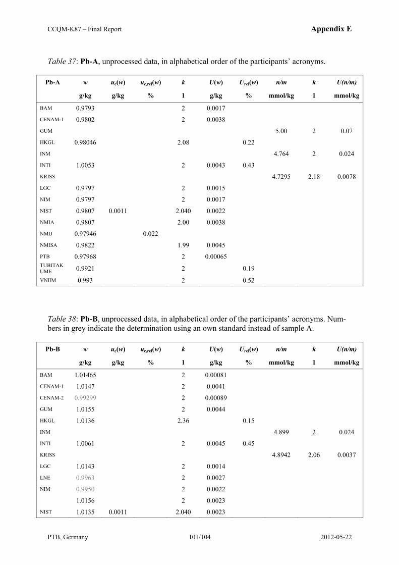
CCQM-K87 – Final Report Appendix E
PTB, Germany 101/104 2012-05-22
Table 37: Pb-A, unprocessed data, in alphabetical order of the participants’ acronyms.
Pb-A w uc(w) uc,rel(w) k U(w) Urel(w) n/m k U(n/m)
g/kg g/kg % 1 g/kg % mmol/kg 1 mmol/kg
BAM 0.9793 2 0.0017 CENAM-1 0.9802 2 0.0038 GUM 5.00 2 0.07 HKGL 0.98046 2.08 0.22 INM 4.764 2 0.024 INTI 1.0053 2 0.0043 0.43 KRISS 4.7295 2.18 0.0078 LGC 0.9797 2 0.0015 NIM 0.9797 2 0.0017 NIST 0.9807 0.0011 2.040 0.0022 NMIA 0.9807 2.00 0.0038 NMIJ 0.97946 0.022 NMISA 0.9822 1.99 0.0045 PTB 0.97968 2 0.00065 TUBITAK UME 0.9921 2 0.19
VNIIM 0.993 2 0.52
Table 38: Pb-B, unprocessed data, in alphabetical order of the participants’ acronyms. Num-bers in grey indicate the determination using an own standard instead of sample A.
Pb-B w uc(w) uc,rel(w) k U(w) Urel(w) n/m k U(n/m)
g/kg g/kg % 1 g/kg % mmol/kg 1 mmol/kg
BAM 1.01465 2 0.00081 CENAM-1 1.0147 2 0.0041 CENAM-2 0.99299 2 0.00089 GUM 1.0155 2 0.0044 HKGL 1.0136 2.36 0.15 INM 4.899 2 0.024 INTI 1.0061 2 0.0045 0.45 KRISS 4.8942 2.06 0.0037 LGC 1.0143 2 0.0014 LNE 0.9963 2 0.0027 NIM 0.9950 2 0.0022 1.0156 2 0.0023 NIST 1.0135 0.0011 2.040 0.0023
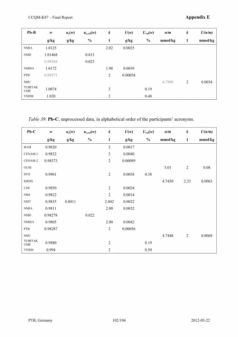
CCQM-K87 – Final Report Appendix E
PTB, Germany 102/104 2012-05-22
Pb-B w uc(w) uc,rel(w) k U(w) Urel(w) n/m k U(n/m)
g/kg g/kg % 1 g/kg % mmol/kg 1 mmol/kg
NMIA 1.0125 2.02 0.0025 NMIJ 1.01468 0.013 0.99384 0.023 NMISA 1.0172 1.98 0.0039 PTB 0.99371 2 0.00058 SMU 4.7989 2 0.0034 TUBITAK UME 1.0074 2 0.19
VNIIM 1.020 2 0.48
Table 39: Pb-C, unprocessed data, in alphabetical order of the participants’ acronyms.
Pb-C w uc(w) uc,rel(w) k U(w) Urel(w) n/m k U(n/m)
g/kg g/kg % 1 g/kg % mmol/kg 1 mmol/kg
BAM 0.9820 2 0.0017 CENAM-1 0.9832 2 0.0040 CENAM-2 0.98373 2 0.00089 GUM 5.01 2 0.08 INTI 0.9901 2 0.0038 0.38 KRISS 4.7430 2.23 0.0063 LNE 0.9850 2 0.0024 NIM 0.9822 2 0.0014 NIST 0.9835 0.0011 2.042 0.0022 NMIA 0.9811 2.00 0.0032 NMIJ 0.98278 0.022 NMISA 0.9805 2.00 0.0042 PTB 0.98287 2 0.00056 SMU 4.7448 2 0.0068 TUBITAK UME 0.9880 2 0.19
VNIIM 0.994 2 0.50
CCQM-K87 – Final Report Appendix F
PTB, Germany 103/104 2012-05-22
Appendix F – Conversion applied to results reported for type B solutions The participants were asked to determine the mass fractions of the elements (E) in type B so-lutions using the according type A solution as the standard assuming a mass fraction of wA,def(E) = 1 g/kg ± 0 g/kg. Those participants applying methods which need no calibrator of the same type as the sample (e.g. coulometric titrimetry) were asked to skip solution type A and report the mass fraction in solution type B against their own standards. Please refer to section 2.1 and appendix A for more details. A few participants determined solutions B against their own standards even though they applied methods requiring calibration solutions of the same type as the sample. To be able to compare all results, those reported as deter-mined against solution A under the above assumption were converted using the KCRV of solution A as the best representation of the “true” value:
)E()E()E(
)E( reportedB,defA,
KCRVA,convB, w
ww
w ⋅= (36)
Appendix G – Molar mass of lead, additional data Figure 2 in section 2.3 shows the molar masses of lead as “reported” by the participants. Sev-eral participants reported individual molar masses for each type of solution. One participant reported the isotope ratios iPb/206Pb. To achieve comparability among all results the reported molar masses and their associated uncertainties were averaged:
3
)Pb()Pb()Pb()Pb( CBA MMMM ++= (37)
( ) ( ) ( ) ( )3
)Pb()Pb()Pb()Pb( C2
B2
A2 MuMuMuMu ++
= (38)
From the isotope ratios Ri/206 the molar mass of lead and its associated uncertainty was calcu-lated (after averaging the isotope ratios) using the GUM Workbench 2.4.
3
206/C,206/B,206/A, iiii
RRRR
++= (39)
[ ])Pb()Pb()Pb()Pb(
1)Pb(
208208
207207
206206
204204
208207206204
MRMRMRMR
RRRRM
+++×
+++=
(40)
Table 40 summarizes all reported data related to the molar mass of lead as well as the molar masses calculated from the data (figure 2).

CCQM-K87 – Final Report Appendix H
PTB, Germany 104/104 2012-05-22
Table 40: Molar masses of lead M(Pb) as reported or calculated using eq. (37)-(40).
Institute M u(M) g/mol g/mol BAM 207.177980 0.000085 CENAM 207.169 0.067 HKGL 207.178 KRISS 207.178 0.040 LGC 207.177834 0.000049 LNE 207.200 0.014 NIM 207.178 NIST 207.18 0.105 NMIA 207.178 0.022 NMIJ 207.1776 0.0009 PTB 207.177797 0.000093 TUBITAK UME 207.177 0.001
Appendix H – Remarks on rounding All results reported, all input quantities of the gravimetric KCRVs, the KCRVs themselves as well as all intermediate results or final results (like DoEs etc.) were handled throughout the complete data processing without any rounding. The data processing was carried out using Microsoft Excel 2007 (15 digits internal precision). Figures showing data were plotted using Origin Lab Corporation Origin 8.5 G SR1. Data transfer from Excel to Origin without round-ing. All numbers printed in this report were rounded usually considering their associated un-certainties in accordance with [7] or in some cases to yield the same number of digits to sim-plify comparability. This means that in rare cases intermediate results cannot be retrieved to their last digits due to the rounding, but this does not influence the accuracy of the printed numbers.