Embed Size (px)
Citation preview

DOCUMENTS DE TRAVAIL / WORKING PAPERS
No 57-2014
The IMACLIM-P Model Version 3.4
Frédéric Ghersi
July 2014
CIRED Working Papers Series
CIRED Centre International de Recherches sur l'Environnement et le Développement
ENPC & CNRS (UMR 8568) / EHESS / AGROPARISTECH / CIRAD / MÉTÉO FRANCE
45 bis, avenue de la Belle Gabrielle F-94736 Nogent sur Marne CEDEX
Tel : (33) 1 43 94 73 73 / Fax : (33) 1 43 94 73 70 www.centre-cired.fr

CIRED Working Papers Series

The IMACLIM models have been developed at CIRED since the 1990’s under Jean-Charles Hourcade‘s
scientific supervision. They currently exist in 3 versions:
A static version, IMACLIM-S, is mostly applied at a national level to produce counterfactual
analyses of environmental fiscal reforms at some historical or projected temporal horizon.
A dynamic, recursive version, IMACLIM-R, articulates growth trajectories for 12 world regions,
based on a back-and-forth dialogue between a succession of static macroeconomic equilibria akin
to those of IMACLIM-S, and a set of sectoral modules framing the evolution of explicit energy
supply and demand technologies.
A prospective version, IMACLIM-P, quite similar to IMACLIM-S, computes the equilibrium
consequences of targeted parameters changes between one historical year and a mid- to long-
term future (rather than between two counterfactual equilibria at a single year, as IMACLIM-S).
This descriptive of IMACLIM-P 3.4 massively draws on that of IMACLIM-S 2.3, from which the model
directly derives. It thus benefits from contributions by Camille Thubin and Emmanuel Combet (cf.
Ghersi et al., 2011).

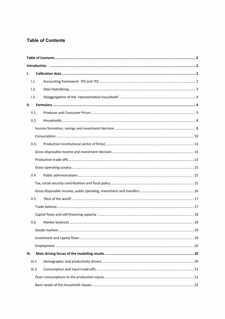
Table of Contents
Table of Contents ............................................................................................................................................. 5
Introduction .................................................................................................................................................. 2
I. Calibration data ...................................................................................................................................... 2
I.1. Accounting framework: TES and TEE ..................................................................................................... 2
I.2. Data Hybridising .................................................................................................................................... 3
I.3. Disaggregation of the ‘representative household’ ................................................................................ 4
II. Formulary ............................................................................................................................................... 4
II.1. Producer and Consumer Prices ............................................................................................................. 5
II.2. Households ............................................................................................................................................ 8
Income formation, savings and investment decision ..................................................................................... 8
Consumption ................................................................................................................................................ 10
II.3. Production (institutional sector of firms) ............................................................................................ 13
Gross disposable income and investment decision...................................................................................... 13
Production trade-offs ................................................................................................................................... 13
Gross operating surplus ................................................................................................................................ 15
II.4. Public administrations ......................................................................................................................... 15
Tax, social security contributions and fiscal policy ....................................................................................... 15
Gross disposable income, public spending, investment and transfers ........................................................ 16
II.5. ‘Rest of the world’ ............................................................................................................................... 17
Trade balance ............................................................................................................................................... 17
Capital flows and self-financing capacity ..................................................................................................... 18
II.6. Market balances .................................................................................................................................. 19
Goods markets ............................................................................................................................................. 19
Investment and capital flows ....................................................................................................................... 19
Employment ................................................................................................................................................. 20
III. Main driving forces of the modelling results ......................................................................................... 20
III.1. Demographic and productivity drivers ................................................................................................ 20
III.2. Consumption and input trade-offs ...................................................................................................... 21
Floor consumptions to the production inputs.............................................................................................. 21
Basic needs of the household classes ........................................................................................................... 22
Production elasticities .................................................................................................................................. 23
Elasticities and functional relationships in the demand system .................................................................. 24
III.3. Other central assumptions .................................................................................................................. 24
International trade ....................................................................................................................................... 24
Public administrations .................................................................................................................................. 25
Other significant behavioural assumptions .................................................................................................. 25
References ................................................................................................................................................ 26
Annex 1 Notations of the model .................................................................................................................... 27
Variables ........................................................................................................................................................... 27
Parameters calibrated on statistical data ......................................................................................................... 30
Exogenous parameters ..................................................................................................................................... 33
Annex 2 Parameterisation of Ghersi and Ricci (2014) .................................................................................... 34
Households trade-offs ...................................................................................................................................... 34
Firms’ trade-offs ............................................................................................................................................... 36
2
Introduction
IMACLIM-P is a direct declination of IMACLIM-S, a computable general equilibrium model (CGEM)
designed to assess the medium- to long-term macroeconomic impacts of aggregate price- or
quantity-based carbon policies, in an accounting framework where economic and physical flows (with
a special focus on energy balances) are equilibrated. IMACLIM-S and IMACLIM-P depart from the
standard neoclassical model in the main feature that their description of the consumers’ and
producers’ trade-offs, and the underlying technical systems, are specifically designed to facilitate
calibration on bottom-up expertise in the energy field, with a view to guaranteeing technical realism
to their simulations of even large mutations of the energy systems.
IMACLIM-P computations resort to the well-known method of “comparative statics” (Samuelson,
1947): they explore the consequences of a change of one or a set of parameters on a set of variables,
in a system of balanced equations. But they come with a twist: rather than computing counterfactual
equilibria at some unique time horizon (as IMACLIM-S does), they compute future equilibria by
considering changes of the main energy/economy growth determinants: demographics, labour
productivity and international energy prices. The insights provided are valid under the assumption
that the transition from the historical (statistical) equilibrium to its projected counterpart is
completed after a series of technical and behavioural adjustments, whose scope are embedded in
the production and consumption elasticities retained. The transition process in itself is however not
described, but implicitly supposed to be smooth enough to prevent multiple equilibria, hysteresis
effects, etc.
This working paper describes the 3.4 version of IMACLIM-P, derived from the 2.3 version of IMACLIM-
S implemented to sustain an expertise about a French carbon tax (Hourcade et al., 2009). It is applied
to 2006 France, whose economy is aggregated in 9 productions and 5 household classes. Section I
synthesises the data sources and calibration procedure. Section II gives a comprehensive formulary,
in a generalised n-good and m-household-class format—with a few exceptions warranted by the
specific treatment of energy sectors. Section III clarifies the driving forces of the model’s projections.
Annexes group a comprehensive listing of notations and the particular values of key parameters of
the model mobilised in Ghersi and Ricci (2014).
I. Calibration data
I.1. Accounting framework: TES and TEE
National accounting statistics provide a comprehensive numerical framework for computable general
equilibrium models. In its 3.4 version, devised to project 2006 France to mid- to long-term horizons,
3
IMACLIM-P is mainly calibrated on aggregated data from two synthesis tables produced by the
French National Institute of Statistics and Economic Studies (INSEE):
The TES (Tableau Entrées-Sorties, input-output table) balances the uses and resources of
products—up to 116 of them in its most disaggregated version.
The TEE (Tableau Économique d’Ensemble) details the primary and secondary distribution of
income between 6 ‘institutional sectors’, i.e. aggregate economic agents: financial firms, non-
financial firms, households, non-profit organisations, public administrations, ‘rest of the world’.
Raw TES data are processed to obtain a description of production and consumption in a
‘product product’ (rather than product branch) system, with no accumulation of stocks.
Supplementary INSEE tables provide extra detail on the components of the value-added—more
specifically a disaggregation of payroll taxes from labour costs, and of fixed capital consumption from
the gross operative surplus.
The TEE is aggregated into 4 institutional sectors (households, firms, public administrations and ‘rest
of the world’), and its many entries are simplified into a set of transfers at a level of aggregation
comparable to that of the TES. Its use allows extending the traditional framework of general
equilibrium modelling to the distribution of national income between economic agents, the resulting
changes in the financial positions of those agents, and the corresponding debt payments.
I.2. Data Hybridising
Considering its focus on energy/economy interactions, IMACLIM-P requires a high degree of realism
in the description of the energy inputs to production and the energy consumptions of households.
Explicit physical energy quantities are poorly represented by the quasi-quantities commonly obtained
from economic data through the normalisation of output prices, and the “single-price” assumption.1
Therefore, a rigorous calibration of the model requires some accurate accounting of the physical
quantities of energy consumed, expressed in a relevant unit (e.g. million-tons-of-oil-equivalent,
MTOE).
Such an accounting is found in the energy balances of the International Energy Agency (IEA). It is also
possible to gather from various sources (IEA, French Comité Professionnel du Pétrole—CPDP, PEGASE
database from the French Ministry of Industry, etc.) prices for each type of energy, or aggregate
thereof, which are indeed agent-specific. The term-by-term product of energy balances and agent-
specific prices defines a matrix of energy consumptions in monetary terms, which does not match
that embedded in the TES for energy products, for a variety of reasons (the inclusion of services
beyond the sheer energy consumptions, the heterogeneity of products, biases from the statistical
balancing methods, etc.). Hybridisation of the TES then consists in imputing the differences between
the values found in the TES, and those computed from energy statistics, to some non-energy good—
in the model with 9 products, to the aggregate composite good. For lack of a better hypothesis the
value-added of the energy products are corrected pro-rata this imputation. In this way, the product
1 Standard CGE models assume that all agents face identical net-of-tax prices for all goods. This is an obvious shortcoming
when it comes to energy markets, where firms and households face quite different conditions.
4
disaggregation is amended, while the total uses and resources across the 9 production sectors are
kept consistent with the original statistics.
The calibration of the model on this hybrid TES eventually leads it to depict (i) volumes of the non-
energy goods that are standardly derived from the single-(normalised)-price assumption, and (ii)
volumes and prices of the energy goods that are strictly aligned on the available statistics. The
differences in price of the same energy good from one agent to the other (e.g. the difference in price
of a kWh of electricity for a firm vs. a household) are accounted for by calibrating ‘specific margins’ to
the different uses.
I.3. Disaggregation of the ‘representative household’
The disaggregation of the ‘representative household’ in 5 living-standard2 classes is based on an
extrapolation of the 2006 Budget de Famille Households Expenditure survey by INSEE, which
extensively covers the resources and uses of 10,240 French households. Combet (2007) largely
documents calibration on an earlier version of the Budget de Famille survey—its descriptive is still to
be updated.
II. Formulary
IMACLIM-P, a comparative statics model from a mathematical point-of-view, boils down to a set of
simultaneous equations:
f1 (x1,..., xn, z1,..., zm) = 0
f2 (x1,..., xn, z1,..., zm) = 0
...
fn (x1,..., xn, z1,..., zm) = 0
with:
xi, i [1, v], a set of variables (as many as equations),
zi, i [1, p], a set of parameters,
fi, i [1, v], a set of functions, some of which are non-linear in xi.
The fi constraints are of two quite different natures: one subset of equations describes accounting
constraints that are necessarily verified to ensure that the accounting system is properly balanced;
the other subset translates various behavioural constraints, written either in a simple linear manner
(e.g. households consume a fixed proportion of their income) or in a more complex non-linear way
2 Surveyed households are ranked according to their disposable income per consumption unit (1 for the first adult + 0.5 per
other adult + 0.3 per child below 14 following the OECD equivalence scale), then separated in quintiles.
5
(e.g. the trade-offs of firms and households). It is these behavioural constraints that ultimately
reflect, in the flexible architecture of IMACLIM-P, a certain economic ‘worldview’.
The presentation of the equations successively details the accounting construction of the set of
relative prices (section II.1), the accounting and behavioural equations that govern the four
institutional sectors represented (households, firms, public administrations and the ‘rest of the
world’, sections 0 to II.5) and the market clearing conditions (section II.6). For reference purposes,
variables and parameters are listed and described in a first appendix. A second appendix details the
values of central parameters used in Ghersi and Ricci (2014). Any variable name indexed with a ‘0’
designates the specific value taken by the variable in the 2006 equilibrium (i.e. the value calibrated
on either the 2006 hybrid TES or the 2006 TEE); it thus indicates a parameter of the equation system.
Although most equations are written in a generalised n-goods m-household classes format, when
necessary good-specific variables are indexed by the following subscripts:
COMP For the composite good (an aggregate of all goods not specifically described).
TRANS For a transportation good, in the market sense i.e. excluding transportation by personal means
(cars, two-wheelers or soft modes).
LOG For a housing good calibrated on expenses encompassing real and imputed rents, with quintile-
specific prices that allow matching actual housing surface statistics.
BAT For a construction good, which encompasses housing maintenance and renovation.
EPRIM For a fossil energy good aggregating crude oil and a small amount of coal.
CARB For vehicle fuels (including liquefied gases used as such).
RAFF For other refined petroleum products (including liquefied gases not used as vehicle fuels).
ELEC For electricity.
GAZ+ For natural gas and heat.
II.1. Producer and Consumer Prices
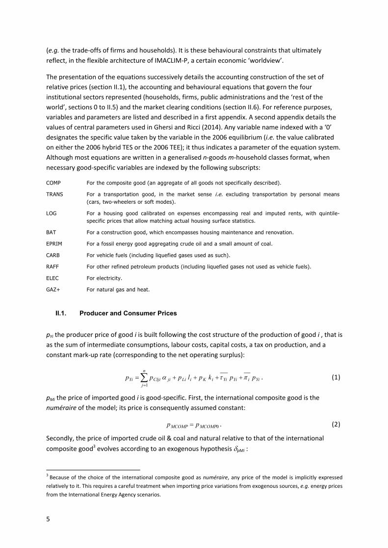
pYi the producer price of good i is built following the cost structure of the production of good i , that is
as the sum of intermediate consumptions, labour costs, capital costs, a tax on production, and a
constant mark-up rate (corresponding to the net operating surplus):
YiiYiYiiKiLi
n
jjiCIjiYi ppkplppp
1
. (1)
pMi the price of imported good i is good-specific. First, the international composite good is the
numéraire of the model; its price is consequently assumed constant:
0MCOMPMCOMP pp . (2)
Secondly, the price of imported crude oil & coal and natural relative to that of the international
composite good3 evolves according to an exogenous hypothesis pMi :
3 Because of the choice of the international composite good as numéraire, any price of the model is implicitly expressed
relatively to it. This requires a careful treatment when importing price variations from exogenous sources, e.g. energy prices
from the International Energy Agency scenarios.
6
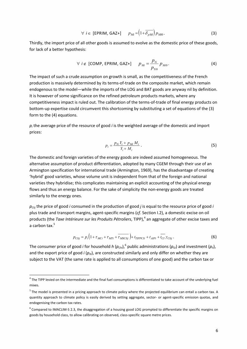
i [EPRIM, GAZ+] 01 MipMiMi pp . (3)
Thirdly, the import price of all other goods is assumed to evolve as the domestic price of these goods,
for lack of a better hypothesis:
i [COMP, EPRIM, GAZ+] 0
0
Mi
Yi
YiMi p
p
pp . (4)
The impact of such a crude assumption on growth is small, as the competitiveness of the French
production is massively determined by its terms-of-trade on the composite market, which remain
endogenous to the model—while the imports of the LOG and BAT goods are anyway nil by definition.
It is however of some significance on the refined petroleum products markets, where any
competitiveness impact is ruled out. The calibration of the terms-of-trade of final energy products on
bottom-up expertise could circumvent this shortcoming by substituting a set of equations of the (3)
form to the (4) equations.
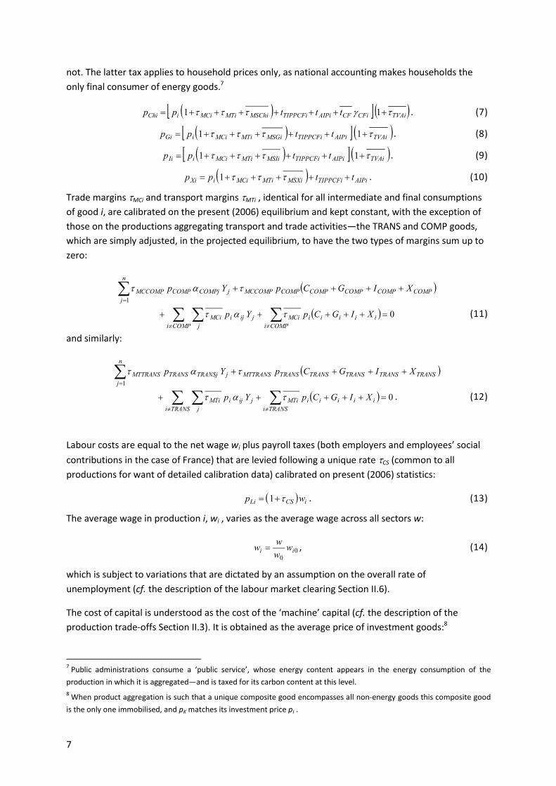
pi the average price of the resource of good i is the weighted average of the domestic and import
prices:
ii
iMiiYii
MY
MpYpp
. (5)
The domestic and foreign varieties of the energy goods are indeed assumed homogeneous. The
alternative assumption of product differentiation, adopted by many CGEM through their use of an
Armington specification for international trade (Armington, 1969), has the disadvantage of creating
‘hybrid’ good varieties, whose volume unit is independent from that of the foreign and national
varieties they hybridise; this complicates maintaining an explicit accounting of the physical energy
flows and thus an energy balance. For the sake of simplicity the non-energy goods are treated
similarly to the energy ones.
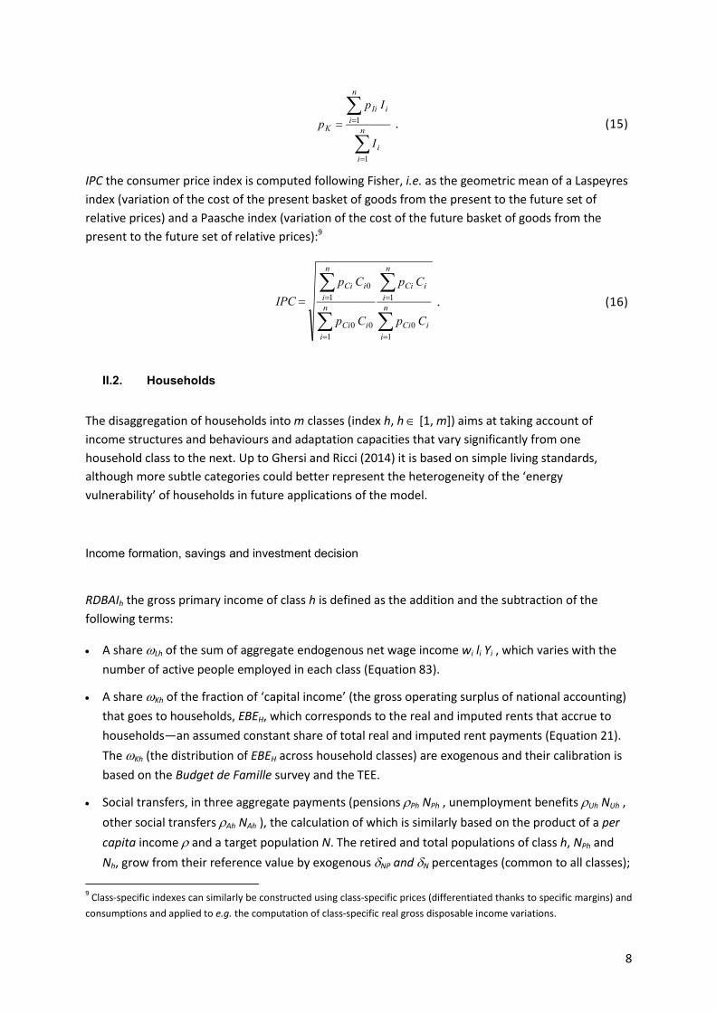
pCIij the price of good i consumed in the production of good j is equal to the resource price of good i
plus trade and transport margins, agent-specific margins (cf. Section I.2), a domestic excise on oil
products (the Taxe Intérieure sur les Produits Pétroliers, TIPP),4 an aggregate of other excise taxes and
a carbon tax.5
CIijCIAIPiTIPPCIiMSCIijMTiMCiiCIij tttpp 1 . (6)
The consumer price of good i for household h (pChi),6 public administrations (pGi) and investment (pIi),
and the export price of good i (pXi), are constructed similarly and only differ on whether they are
subject to the VAT (the same rate is applied to all consumptions of one good) and the carbon tax or
4 The TIPP levied on the intermediate and the final fuel consumptions is differentiated to take account of the underlying fuel
mixes.
5 The model is presented in a pricing approach to climate policy where the projected equilibrium can entail a carbon tax. A
quantity approach to climate policy is easily derived by setting aggregate, sector- or agent-specific emission quotas, and
endogenising the carbon tax rates.
6 Compared to IMACLIM-S 2.3, the disaggregation of a housing good LOG prompted to differentiate the specific margins on
goods by household class, to allow calibrating on observed, class-specific square metre prices.
7
not. The latter tax applies to household prices only, as national accounting makes households the
only final consumer of energy goods.7
TVAiCFiCFAIPiTIPPCFiMSChiMTiMCiiChi tttpp 11 . (7)
TVAiAIPiTIPPCFiMSGiMTiMCiiGi ttpp 11 . (8)
TVAiAIPiTIPPCFiMSIiMTiMCiiIi ttpp 11 . (9)
AIPiTIPPCFiMSXiMTiMCiiXi ttpp 1 . (10)
Trade margins MCi and transport margins MTi , identical for all intermediate and final consumptions
of good i, are calibrated on the present (2006) equilibrium and kept constant, with the exception of
those on the productions aggregating transport and trade activities—the TRANS and COMP goods,
which are simply adjusted, in the projected equilibrium, to have the two types of margins sum up to
zero:
COMPCOMPCOMPCOMPCOMPMCCOMP
n
j
jCOMPjCOMPMCCOMP XIGCpYp
1
0 COMPi
iiiiiMCi
COMPi j
jijiMCi XIGCpYp (11)
and similarly:
TRANSTRANSTRANSTRANSTRANSMTTRANS
n
j
jTRANSjTRANSMTTRANS XIGCpYp
1
0 TRANSi
iiiiiMTi
TRANSi j
jijiMTi XIGCpYp . (12)
Labour costs are equal to the net wage wi plus payroll taxes (both employers and employees’ social
contributions in the case of France) that are levied following a unique rate CS (common to all
productions for want of detailed calibration data) calibrated on present (2006) statistics:
iCSLi wp 1 . (13)
The average wage in production i, wi , varies as the average wage across all sectors w:
00
ii ww
ww , (14)
which is subject to variations that are dictated by an assumption on the overall rate of
unemployment (cf. the description of the labour market clearing Section II.6).
The cost of capital is understood as the cost of the ‘machine’ capital (cf. the description of the
production trade-offs Section II.3). It is obtained as the average price of investment goods:8
7 Public administrations consume a ‘public service’, whose energy content appears in the energy consumption of the
production in which it is aggregated—and is taxed for its carbon content at this level.
8 When product aggregation is such that a unique composite good encompasses all non-energy goods this composite good
is the only one immobilised, and pK matches its investment price pI .
8
n
i
i
n
i
iIi
K
I
Ip
p
1
1 . (15)
IPC the consumer price index is computed following Fisher, i.e. as the geometric mean of a Laspeyres
index (variation of the cost of the present basket of goods from the present to the future set of
relative prices) and a Paasche index (variation of the cost of the future basket of goods from the
present to the future set of relative prices):9
n
i
iCi
n
i
iCi
n
i
iCi
n
i
iCi
Cp
Cp
Cp
Cp
IPC
1
0
1
1
00
1
0
. (16)
II.2. Households
The disaggregation of households into m classes (index h, h [1, m]) aims at taking account of
income structures and behaviours and adaptation capacities that vary significantly from one
household class to the next. Up to Ghersi and Ricci (2014) it is based on simple living standards,
although more subtle categories could better represent the heterogeneity of the ‘energy
vulnerability’ of households in future applications of the model.
Income formation, savings and investment decision
RDBAIh the gross primary income of class h is defined as the addition and the subtraction of the
following terms:
A share Lh of the sum of aggregate endogenous net wage income wi li Yi , which varies with the
number of active people employed in each class (Equation 83).
A share Kh of the fraction of ‘capital income’ (the gross operating surplus of national accounting)
that goes to households, EBEH, which corresponds to the real and imputed rents that accrue to
households—an assumed constant share of total real and imputed rent payments (Equation 21).
The Kh (the distribution of EBEH across household classes) are exogenous and their calibration is
based on the Budget de Famille survey and the TEE.
Social transfers, in three aggregate payments (pensions Ph NPh , unemployment benefits Uh NUh ,
other social transfers Ah NAh ), the calculation of which is similarly based on the product of a per
capita income and a target population N. The retired and total populations of class h, NPh and
Nh, grow from their reference value by exogenous NP and N percentages (common to all classes);
9 Class-specific indexes can similarly be constructed using class-specific prices (differentiated thanks to specific margins) and
consumptions and applied to e.g. the computation of class-specific real gross disposable income variations.
9
the number of unemployed NUh endogenously derives from the conditions on the labour market
(Equation 82).
An exogenous share ATh of (small) residual transfers ATH , which correspond to the sum of “other
current transfers” and “capital transfers”, accounts D7 and D9 of the TEE.
A ‘debt service’ iH Dh , which is indeed negative and corresponds to property income (account D4
of the TEE: interests, dividends, real estate revenues, etc.) for most if not all income classes
(depending on the extent of class disaggregation). This service is the product of the households’
net debt Dh , the evolution of which is explained below (Equation 26), and an endogenous
effective interest rate iH (cf. Equation 76).
Hence
01 PhNPPh NN , (17)
01 hNh NN , (18)
hhTHAThhAhUhUhPhPhHKh
n
i
iiiLhh DiANNNEBEYlwRDBAI
1
, (19)
with ATH a constant share ATH of AT (cf. Equation 74) and EBEH, which is massively composed of
imputed rents, a constant share KH of pLOG LOG:
TATHTH AA (20)
LOGpEBE LOGKHH (21)
The gross disposable income RDBh of class h is obtained by subtracting from RDBAIh the income tax
TIRh levied at a constant average rate (Equation 56), and other direct taxes Th that are indexed on IPC
(Equation 57). Rh , the consumption budget of class h, is inferred from disposable income by
subtracting savings. The savings rate τSh is exogenous (calibrated to accommodate the values of RDBh
and Rh in the present equilibrium).
hIRhhh TTRDBAIRDB (22)
hShh RDBR 1 (23)
A further exploration of the data available in the TEE gives households’ investment FBCFh (Formation
Brute de Capital Fixe, i.e. Gross Fixed Capital Formation) as distinct from their savings; FBCFh is
assumed to follow the simple rule of a fixed ratio to gross disposable income (Equation 24). The
difference between savings and investment gives the self-financing capacity (SFC) of class h, CAFh.
0
0
h
h
h
h
RDB
FBCF
RDB
FBCF (24)
hhShh FBCFRDBCAF (25)
The evolution of CAFh between the present and future equilibrium can then be used to estimate the
evolution of net debt Dh . The computation is based on the simple assumption that the average SFC
over the years of projection tPROJ is a mean of the present and future SFC.
10
2
00
hhPROJhh
CAFCAFtDD
(26)
Consumption
Representing households trade-offs requires both supplementary good disaggregations and good
aggregations in intermediate consumption bundles. The following consumptions are thus added to
the 9 productions distinguished by the model:
ELEC1 The specific (non-substitutable) share of electricity consumptions—calibrated on
quintile-specific data from a 2006 Housing Survey by INSEE (the Enquête Logement).
ELEC2 Any ELEC not resorting to ELEC1, i.e. the non-specific, substitutable electricity
consumptions covering space heating, water heating and cooking.
TRANS1 The share of the consumption of public transports constrained by the housing location
choice (public transports share of daily transportation needs including, but not limited
to, commuting)—calibrated on quintile-specific data from a 2006 Transport survey by
INSEE (the Enquête Transports).
TRANS2 Any TRANS not resorting to TRANS1, i.e. leisure-motivated public transports (including
aviation).
CARB1 The share of the consumption of automotive fuels constrained by the housing location
choice (automotive share of daily transportation needs including, but not limited to,
commuting)—calibrated on quintile-specific data from a 2006 Transport survey by
INSEE (the Enquête Transports).
CARB2 Any CARB not resorting to CARB1, i.e. leisure-motivated automotive fuel consumption
(including aviation).
TCONT A bundle of TRANS1 and CARB1, aggregated through a CES specification above a floor
consumption (cf. infra). Arbitrary 2006 value (without impact on modelling results).
TLOIS A bundle of TRANS2 and CARB2, aggregated through a CES specification above a floor
consumption (cf. infra). Arbitrary 2006 value (without impact on modelling results).
CONS A bundle of TLOIS and COMP, aggregated through a CES specification above a floor
consumption (cf. infra). Arbitrary 2006 value (without impact on modelling results).
EDNS A bundle of ELEC2, RAFF and GAZ+, aggregated through a CES specification above a
floor consumption, and modified by exogenous trends (cf. infra).
SEDNS A CES bundle of EDNS and BAT.
11
At the core of their consumption trade-offs, households devote a constant share of their
consumption budget R (we drop the class index h for the sake of readability) to housing expenses pLOG
LOG:
R
LOGp
R
LOGp LOGLOG 00 , (27)
which amounts to considering, following the conclusions of urban economics synthesised by Fujita
(1989), that a Cobb-Douglas utility function governs consumer choices between square metres of
housing and other expenses. The evolution of the demand for housing square metres mechanically
induces that of the constrained share of households transport demand, TCONT, based on some
assumption on the minimum housing surface LOG LOG0:
TCONTb
LOG
TCONT
LOG
LOG
R
TCONTp
0
1
(28)
with LOG the proportion of the present housing surface LOG0 that corresponds to the minimum
housing surface and bTCONT a coefficient calibrated on present (2006) data.
Similarly to the way it implies TCONT, LOG mechanically induces a consumption of substitutable
energy services SEDNS. The relationship is assumed isoelastic, following an exogenous elasticity bSEDNS
of SEDNS demand to LOG:
SEDNSbSEDNS LOGaSEDNS (29)
with aSEDNS calibrated on present data (SEDNS can be normalised without impact on modelling
results).
By contrast, specific electricity consumptions ELEC1, calibrated on data from a 2006 Housing Survey
by INSEE (the Enquête Logement), are supposed isoelastic to total population with elasticity bELEC1 (cf.
Annex 2):
111 ELECb
ELEC NaELEC , (30)
with aELEC1 calibrated on present (2006) data, ELEC1 being expressed as million tons-of-oil-equivalent
(as all other energy consumptions following data hybridising, cf. Section I.2).
All other trade-offs are settled by CES (Constant Elasticity of Substitution) specifications, but only
beyond floor consumptions that are meant to represent ‘basic needs’, thereby enhancing the ability
of the consumption model to calibrate on bottom-up expertise (following Ghersi and Hourcade,
2006).10 This concerns the trade-off between TRANS1 and CARB1 in TCONT; that between TLOIS and
COMP in CONS; that between ELEC2, RAFF and GAZ+ in EDNS; that between EDNS and BAT (in a quite
specific version, cf. infra) in SEDNS. For these trade-offs, if the goods (or bundles) A, B and C are
substitutable within some aggregate X, then the optimal consumption of good A (that minimising the
budget necessary to form X) is:
10
It is thus only the flexible shares of consumptions that substitute following a constant elasticity. The substitution
elasticities of total consumption volumes are decreasing with total consumption volumes.
12
CBAjCjj
CA
AXAAA
XX
X
pp
RCC,,
10
(31)
with βA CA0 the basic need of good A; pCi the consumer price of good i; X the substitution elasticity of
the consumptions of A, B and C for the shares superseding their basic needs; j a set of coefficients
calibrated on the present budget structures; RX the consumption budget of good X. As an exception,
CEDNS the consumption of substitutable residential energy is modified by a supplementary exogenous
trend that combines assumptions on the efficiency of the post-2006 building stock and on specific
electricity consumption: the (1-aHEAT) share of projected EDNS consumption devoted to cooking and
water heating is supposed to progress as population N; assuming a δLOG depreciation rate, the aHEAT
share of projected EDNS is unmodified for a share (1-δLOG)tPROJ representing the pre-2006 stock
remaining in 2035 but it is cut down by a ωHEAT efficiency factor symbolising strengthened building
regulations for the post-2006 construction (in this equation we reintroduce the class index h to make
clear that aHEAT, δLOG and ωHEAT are not class-specific):
0
0 11
1h
hHEAT
h
ht
LOGhHEAT
tLOGHEATEDNSh
N
Na
LOG
LOGLOGaC
PROJ
PROJ
BATEDNSjCjj
CEDNS
EDNSSEDNSEDNSEDNS
SEDNSSEDNS
SEDNS
pp
RC,
10
(32)
RX is straightforwardly defined as:
XCXX CpR (33)
with the exception of RCONS, which is defined to acknowledge the aggregate budget constraint, as R
the total consumption budget minus all expenses but these on COMP and TLOIS (TRANS2 and
CARB2):
2,2, CARBTRANSCOMPX
XCXCONS CpRR (34)
At last, the CES price of aggregate X follows the textbook formula
X
X
XX
CBAjCjjCX pp
1
,,
1
(35)
where for the sake of convenience
X
XX
1 (36)
Note at last that EPRIM the consumption of primary fossil fuels boils down to a residual consumption
of coal in 2006, which disappears from statistics in 2007. For this reason projected EPRIM
consumptions are arbitrarily fixed to 0 across all household classes.
13
II.3. Production (institutional sector of firms)
Gross disposable income and investment decision
Similar to that of households, the firms’ disposable income RDBS is defined as the addition and
subtraction of:
An exogenous share KS of capital income i.e. EBE (cf. Equation 47),
A ‘debt service’ (interests, dividends) iS DS , which is strongly positive in the present equilibrium
(firms are net debtors in 2006), and served at an interest rate iS that varies in the same way as iH
(Equation 76),
Corporate tax payments TIS ,
And an exogenous share ATS of other transfers AT, which are assumed a constant share of GDP
(Equation 74).
TATSISSSKSS ATDiEBERDB . (37)
The ratio of the gross fix capital formation of firms FBCFS to their disposable income RDBS is assumed
constant; similar to households and in accordance with national accounting their self-financing
capacity CAFS then arises from the difference between RDBS and FBCFS. The net debt of firms DS is
then calculated from their CAFS following the same specification as that applied to households.
0
0
S
S
S
S
RDB
FBCF
RDB
FBCF . (38)
SSS FBCFRDBCAF . (39)
2
00
SSPROJSS
CAFCAFtDD
. (40)
Production trade-offs
For reasons similar to those presented for the demand of households, the production trade-offs,
which are the subject of a specific publication (Ghersi and Hourcade, 2006), are limited by technical
asymptotes that constrain the unit consumptions of factors above some floor values. Compared to
Ghersi and Hourcade (2006) the restrictive assumption is made that the variable shares of the unit
consumptions of the 11 factors (9 secondary inputs, labour and capital) are substitutable according
to a CES specification—similar to household consumption, the existence of a fix share of each of
these consumptions implies that the elasticities of substitution of total unit consumptions (sum of
the fix and variable shares) are not fixed, but decrease as the consumptions approach their
asymptotes.
Under these assumptions and constraints, the minimisation of unit costs of production leads to a
formulation of the unitary consumptions of secondary factors αji , of labour li and of capital ki which
14
can be written as the sum of the floor value and a consumption above this value. The latter
corresponds to the familiar expression of conditional factor demands of a CES production function
with an elasticity of i (the coefficients of which, CIij, Li0 and Ki0 , are calibrated in the present
equilibrium).
i
ii
i
iii
i
KKii
LiLi
n
jCIjiji
CIji
jijijiiji p
pp
p
1
11
1
10 (41)
i
ii
i
iii
i
KKii
LiLi
n
jCIjiji
Li
iLiiLi
i
ii p
pp
pll
1
11
1
10 (42)
i
ii
i
iii
i
KKii
LiLi
n
jCIjiji
Ki
KiiKiii p
pp
pkk
1
11
1
10 , (43)
where for convenience
i
ii
1 . (44)
This sum is however modified to take into account the combination of an exogenous labour
productivity improvement factor i ,11 and of endogenous decreasing returns i . The latter impact all
factor consumptions by assuming them elastic to the volume produced, by a fixed elasticity Yi ,
which is calibrated under the assumption of marginal cost pricing.
Yi
i
ii
Y
Y
0
(45)
i
iYi
1. (46)
Let us emphasise again that the ‘cost of capital’ pK entering the trade-offs is stricto sensu the price of
‘machine capital’, i.e. equal to a simple weighted sum of the investment prices of immobilised goods
(Equation 15), and unrelated to the interest rates charged on financial markets: on the one hand
production trade-offs are based upon the strict cost of inputs, including that of physical capital ki
(calibrated on the consumption of fixed capital of the TES); on the other hand, notwithstanding this
arbitrage, the firms’ activity and a rule of self-investment (FBCFS , Equation 38) lead to a change in
their financial position DS , whose service is not assumed to specifically weigh on physical capital as
an input.
11
In IMACLIM-S the i designate an endogenous growth coefficient that links factor consumptions (not only labour but all
of them, following a Hicks-neutral hypothesis) to production levels. This specification is irrelevant to the exogenous growth
framework of IMACLIM-P.
15
Gross operating surplus
Capital consumptions, constant rates of operating margin i and specific margins MS determine the
gross operating surplus (Excédent Brut d’Exploitation, EBE):
S
n
iiYiiiiKi MYpYkpEBE
1
(47)
This EBE, which corresponds to capital income, is split between agents following constant shares
(calibrated on the present equilibrium). By construction, the specific margins on the different sales
MS sum to zero in the present equilibrium (this is a constraint of the hybridising process), however
they do not in the future equilibrium, their constant rates being applied to varying prices. Their
expression is then:
iiiMSXiiMSG
hhiiMSCh
jjijiMSCIS XpGpCpYpM
iiiij (48)
II.4. Public administrations
Tax, social security contributions and fiscal policy
Tax and social security contributions form the larger share of government resources. In this 3.4
version of IMACLIM-P, all tax rates other than the carbon tax are supposed constant, while excise
taxes are scaled up by the consumer price index IPC:
X [CI, CF] 0TIPPXiTIPPXi tIPCt , (49)
0AIPiAIPi tIPCt . (50)
The various tax revenues are defined by applying these rates to their respective bases:
n
iiYiYY YpT
i
1
, (51)
n
iiiiTIPPCF
n
i
n
jijiTIPPCITIPP IGCtYtT
iji
11 1
, (52)
n
iiiiAIP
n
i
n
jijiAIPAIP IGCtYtT
ij
11 1
, (53)
n
iiIiiGiiCi
TVA
TVATVA IpGpCpT
i
i
1 1
, (54)
SISIS EBET , (55)
DBAIhIRhIRh RT . (56)
16
Similar to excise taxes and for lack of more detail on its composition the sum of households’ direct
taxes other than the income tax TIR is assumed to grow as the general price level:
0hh TIPCT . (57)
The sum of social contributions TCS follows the same logic as other tax revenues again:
n
iiiiCSCS YlwT
1
. (58)
So does the carbon on intermediate consumptions (tCI) and on final consumptions (tCF) except that it
is exogenous:
n
iiCFiCF
n
i
n
jijiCIjiCICARB CtYtT
11 1
. (59)
In the dynamic framework of IMACLIM-P the ‘budget neutrality’ condition of counterfactual analyses
is reinterpreted as a constraint on public debt accumulation, enforced as a constant ratio of public
debt to GDP (Equation 43b). The variables that adjust to meet this constraint are the per capita social
transfers ρU, ρP and ρA, which are scaled up or down by a common factor. In the case when a carbon
tax provides supplementary tax income, the pressure on these transfers is lessened.
0
0
PIB
D
PIB
D GG (60)
At last, T is the sum of taxes and social contributions:
CARB
m
hh
m
hIRhISTVAAIPTIPPYCS TTTTTTTTTT
11
(61)
Gross disposable income, public spending, investment and transfers
Similar to households and firms (following the logic prevailing in the TEE), the gross disposable
income of public administrations RDBG is the sum of taxes and social contributions, of exogenous
shares KG of EBE and ATG of ‘other transfers’ AT , from which are subtracted public expenditures
pG G , a set of social transfers RP , RU and RA , and a debt service iG DG :
GGAUP
n
iiGiTATGKGG DiRRRGpAEBETRDB
1
(62)
Public expenditures pG G are assumed to keep pace with national income and are therefore
constrained as a constant share of GDP:
0
100
1
PIB
Gp
PIB
Gpn
iiGi
n
iiGi
, (63)
Social transfers RP , RU and RA are the sum across household classes of the transfers defined as
components of their before-tax disposable income (Equation 19):
17
m
hPhPhP NR
1
(64)
m
hUhUhU NR
1
(65)
m
hhAhA NR
1
, (66)
with per capita transfers P , U and A variables of the model aimed at the constraint on public debt
(Equation 43).
At last, the interest rate iG of public debt evolves as do iH and iS (Equation 76).
Public investment FBCFG , same as public expenditures pG G, is supposed to mobilise a constant share
of GDP. Subtracting it from RDBG produces CAFG , which determines the variation of the public debt:
0
0
PIB
FBCF
PIB
FBCF GG (67)
GGG FBCFRDBCAF (68)
2
00
GGPROJGG
CAFCAFtDD
(69)
II.5. ‘Rest of the world’
Trade balance
Competition on international markets is settled through relative prices. The ratio of imports to
domestic production on the one hand, and the ‘absolute’ exported quantities on the other hand, are
elastic to the terms of trade, according to constant, product-specific elasticities:
Mpi
Mi
Yi
Yi
Mi
i
i
i
i
p
p
p
p
Y
M
Y
M
0
0
0
0 (70)
XiMi
Xi
Xi
Mi
i
iXpi
p
p
p
p
X
X
1
0
0
0
(71)
The different treatment of imports and exports merely reflects the assumption that, notwithstanding
the evolution of the terms of trade, import volumes rise in proportion to domestic economic activity
(domestic production), while exports are impacted by global growth. The latter fact is captured by
assuming an extra, exogenous Xi increase of volumes exported. In total, as far as exports are
concerned France is depicted as supplying a terms-of-trade elastic share of a Xi expanded
international market.
18
The only exception to this terms-of-trade treatment is the international market for primary fossil
energies EPRIM. Considering the paucity of France in such resources domestic EPRIM production is
arbitrarily set to 0 in the projected equilibrium, and the imports are assumed to mechanically balance
the market on the resources’ side.
Capital flows and self-financing capacity
Capital flows from and to the ‘Rest of the World’ (ROW) are not assigned a specific behaviour, but are
simply determined as the balance of capital flows of the three national institutional sectors
(households, firms, public administrations) to ensure the balance of trade accounting. This
assumption determines the self-financing capacity of the ROW, which in turn determines the
evolution of DRDM , its net financial debt:
n
GSHKTK
n
GSHKKK
n
iiXi
n
iiMiRDM ADiXpMpCAF
,,,,11
, (72)
2
00
RDMRDMPROJRDMRDM
CAFCAFtDD
. (73)
By construction the self-financing capacities (SFC) of the 4 agents clear (sum to zero), and accordingly
the net positions, which are systematically built on the SFCs, strictly compensate each other in the
projected as in the present equilibrium—indeed a nil condition on the sum of net positions could be
substituted to equation 73 without impacting the model. The hypothesis of a systematic
‘compensation’ by the ROW of the property incomes of national agents without any reference to its
debt DRDM may seem crude, but in fine only replicates the method of construction of the TEE. Indeed,
in the 2006 calibration equilibrium the effective interest rate of the ROW (ratio of net debt to its
property income), which ultimately results from a myriad of debit and credit positions and from the
corresponding capital flows, is negative—unworkable for modelling purposes.
At last, as previously mentioned other transfers AT (« other current transfers » and « capital
transfers », aggregates D7 and D9 of the TEE) are defined as a fixed share of GDP12:
0
0
PIB
A
PIB
A TT (74)
12
The sum across agents of the D7 and D9 accounts being nil by definition (they aggregate transfers between agents), AT is
in fact calibrated on the sum of the net transfers that are strictly positive. As a consequence the shares ATH, ATS, ATG and
ATRDM , summing to 0 by construction, are ratios properly speaking.
19
II.6. Market balances
Goods markets
Goods market clearing is a simple accounting balance between resources (production and
imports) and uses (intermediate consumption, households and public administrations’ consumption,
investment, exports). Thanks to the process of hybridisation, this equation is written in MTOE for
energy goods and consistent with the 2006 energy balance of the IEA (notwithstanding that the G
and I of energy goods are nil by definition).
iiii
n
jjijii XIGCYMY
1
(75)
Of course the aggregate consumption of households Ci sums up the consumptions of all classes Cih.
Investment and capital flows
The effective interest rates iH , iS and iG faced by households, firms and public administrations, settle
to balance capital markets: their shift from a common point differential i (Equation 67) impacts the
households’ and firms’ disposable incomes RDBH and RDBS , hence their investment decisions FBCFH
and FBCFS , in order to match the supply of capital they correspond to, adding up to the public GFCF
FBCFG , to the demand for investment goods pIi Ii (Equation 77). This demand is in turn constrained by
the assumption that the ratio of each of its real components Ii to total fixed capital consumption (the
sum of ki Yi) is constant. In other words, the capital immobilised in all productions is supposed
homogeneous, and all its components vary as the total consumption of fixed capital.
K [H, S, G] iKK ii 0 (76)
n
iiIi
GSHKK IpFBCF
1,,
(77)
n
jjj
in
jjj
i
Yk
I
Yk
I
100
0
1
(78)
Therefore the closure of the model is on the investment supply of agents, which mechanically adapts
to the investment demand from productions. Through an adjustment of interest rates it leads to
fluctuations in financial flows between creditors and debtors, and eventually in some evolution of
their net financial positions.
20
Employment
The labour market results from the interplay of labour demand from the production systems, equal
to the sum of their factor demands li Yi , and of labour supply from households. The labour
endowment of households L0 grows by an exogenous, common rate L, calibrated on the total full-
time equivalent of the active population in the present and future equilibrium. However the model
allows for a strictly positive unemployment rate u and the market clearing condition writes:
n
iiiL YlLu
10)1()1( . (79)
Rather than explicitly describing labour supply behaviour, the model treats as exogenous the overall
unemployment rate u:
uu . (80)
Changes in employment corresponding to the evolution of u are then split between the household
classes according to their specific unemployment rates uh:
0
0u
uuu hh , (81)
hence NUh the number of unemployed in each class follows:
01 hLhUh LuN . (82)
NLh the number of employed in class h (defined as (1+L) Lh0 – NUh ) allows moreover to determine the
share Lh of total labour income that accrues to class h:
m
hLh
Lh
Lh
LhLh
Lh
Lh
N
N
N
N
10
0
00
. (83)
III. Main driving forces of the modelling results
The future economic conditions projected by IMACLIM-P result from the combination of a series of
assumptions. Some are straightforwardly embodied in some of the parameters of the model. Others
are more intricately implied by some of the model’s equations. This last section discusses the most
significant of them.
III.1. Demographic and productivity drivers
At the core of the model, two demographic and productivity assumptions, together with the
unemployment rate u, can be seen as shaping the potential growth of the projected economy:

21
L the growth of labour supply. It is based on that of the labour force but can embark any
contrasted assumption on the evolution of working hours.
i the 1 × 9 vector of labour productivity growths. Each production can benefit from specific
productivity improvements, although the forecasts available in the literature are generally
not differentiated.
u the unemployment rate, is inseparable from the two former assumptions, for the obvious
reason that it fixes the share of the labour supply that is actively employed.
Two other demographic drivers impact on potential growth by their distributive consequences, as
they define the candidate populations to generic social transfers, and pensions.
N the growth of total population,
NP the growth of the pensioned population.
III.2. Consumption and input trade-offs
Floor consumptions to the production inputs
In intermediate consumption there are floor volumes of the 11 inputs (2 primary facors, 9 secondary
factors) per unit of production. They can be interpreted as technical frontiers that are assumed
insuperable at the tPROJ horizon at which the economy is projected. For instance, for i = CARB and
j = TRANS, ij is the percentage of the 2006 fuel input into one unit of transport service that is
supposed to endure whatever the change in relative prices observed after tPROJ years. It is to be
shaped by combining assumptions on the maximum expected progress in ICE efficiency (including the
possible development of hybrid motorisation) and road-to-rail substitution, but might also consider
some minimum expected development of air transportation, for which no substitutes to
conventional fuels are currently anticipated. Incidentally, the floor input intensities are a useful way
to circumvent the ‘flat’ (rather than nested) nature of the production process of IMACLIM-P, as they
allow fixing input-specific substitution elasticities: with TRANS the elasticity prevailing in the
production of TRANS, the specific substitution elasticity of CARB in TRANS is (1–CARB/TRANS) TRANS.
The floors are grouped into 3 matrices:
CI is the 9 × 9 matrix of intermediate consumption floors (shares of the 2006 consumptions per
unit that remain after tPROJ years notwithstanding relative price changes).
L is the 1 × 9 vector of floors to the labour intensity of productions (shares of the 2006 labour
time per unit that remain after tPROJ years notwithstanding relative price changes).
K is the 1 × 9 vector of floors to the capital intensity of productions (shares of the 2006 fixed
capital consumption per unit that remain after tPROJ years notwithstanding relative price
changes).

22
Basic needs of the household classes
In final consumption, the floor consumptions are class-specific minima to the aggregate consumption
of each class, for each good. They can also be set for aggregates, when the competition between the
goods constituting the aggregate is not to be constrained by floors at their level. The situation of
each aggregate and product is specific enough to warrant clarifications.
COMP: the composite good, although it aggregates with many other goods such essential
consumptions as water, food and clothing, is not assigned any basic need (βCOMP = 0). Considering its
magnitude in current budget structures it is treated as an adjustment variable. It is left to the
modeller to judge if the projected variations in COMP threaten the sustainability of the modelled
scenario.
TRANS1: A βTRANS1 vector of class-specific basic needs (expressed as shares of TRANS10) can be
defined to link a minimal, necessary consumption of public transports with the urban organisation
embodied in the combination of βLOG and βTCONT, the basic housing space and transportation needs of
household classes. The TCONT volume induced by βTRANS1 should be smaller than βCONT, by definition
of the latter (cf. infra).
TRANS2: cf. TRANS1 immediately above, a βTRANS2 vector of class-specific basic needs can be specified,
although by definition ‘leisure’ transportation TLOIS is more open to trade-off than constrained
transportation TCONT.
LOG: A βLOG vector of class-specific basic square-metre needs (expressed as shares of LOG0) is central
to the demand system of the projection. It is to be set in consistency with the βTCONT, βELEC1, βEDNS and
βBAT vectors, to combine into a minimum minimorum to the housing conditions of class h, and its
transportation consequences. Thanks to the hybridising process CLOGh0 / Nh0 is the housing square
metre per person of class h in 2006, and can be used to define the class’s basic need, considering the
growth of its population.
BAT: cf. LOG immediately above. Contrary to LOG, BAT does not have an interpretable physical unit.
Defining basic needs to BAT boils down to making some assumption about the share of observed BAT
consumptions that are unavoidable in the maintenance of βLOG LOG0.
EPRIM: considering the assumption of an EPRIM consumption systematically brought down to 0
there is no need to define any basic need to EPRIM.
CARB1: cf. TRANS1 above, a βCARB1 vector of class-specific basic needs can be defined to link a
minimal, necessary consumption of vehicle fuels with the urban organisation embodied in the
combination of βLOG and βTCONT, the basic housing space and transportation needs of household
classes. The TCONT volume induced by βCARB1 should be smaller than βTCONT TCONT0, by definition of
the latter (cf. infra).
CARB2: cf. TRANS2 above, a βCARB2 vector of class-specific basic needs can be specified, although by
definition ‘leisure’ transportation is more open to trade-off than constrained transportation TCONT.
RAFF: over a temporal horizon compatible with the inertia of heating systems there is no obvious
restriction to the substitutability of gas and electricity to light fuel oil for the heating and cooking
23
purposes backing the RAFF consumptions of households. Still, A βRAFF vector is available to project
over shorter terms, or test more restrictive assumptions.
ELEC1: cf. LOG above. As LOG, ELEC1 is expressed in an interpretable physical unit, namely MTOE. Its
basic needs are best set by assuming some minimal kWh per square-metre consumption of specific
electricity, then converting and scaling up to the aggregate basic need of square metres βLOG LOG0.
ELEC2: cf. RAFF above. βELEC2 is available to set a minimum bound to electric heating and cooking.
GAZ+: cf. RAFF above. βGAZ+ is available to set a minimum bound to gas heating and cooking, and
possibly a network heat component.
CONS: there does not seem to be any reason to define a basic need to CONS other than the volume
produced by the basic need of TLOIS (βCONS = 0).
TCONT: cf. LOG above. TCONT does not have an interpretable physical unit, but is composed of goods
that do, TRANS1 in pkm and CARB1 in MTOE. Basic needs to TCONT are best obtained from
computing what volume of TCONT is produced by ‘polar’ scenarios where the minimum
transportation effort compatible with βLOG LOG0 is realised by exclusive consumptions of TRANS1 or
CARB1.
EDNS: cf. LOG above. EDNS does not have an interpretable physical unit, but is composed of goods
that do, ELEC2, RAFF and GAZ+ in MTOE. Basic needs to EDNS can be obtained from computing the
volume of EDNS produced by basic needs of ELEC2, RAFF or GAZ+, compatible with βLOG LOG0.
SEDNS: there does not seem to be any reason to define a basic need to SEDNS other than the volume
produced by the basic need of EDNS or BAT (βSEDNS = 0).
TLOIS: cf. TCONT above, TLOIS does not have an interpretable physical unit, but is composed of goods
that do, TRANS2 in pkm and CARB2 in MTOE. Basic needs to TLOIS are best obtained from computing
what volume of TLOIS is produced by alternative basic needs of TRANS2 or CARB2. The case for a
basic need to a leisure consumption is of course slimmer than in the case of TCONT.
Production elasticities
At this stage the production function assumed for all productions is a ‘flat’ (rather than nested)
construction that allows differentiating the treatment of the various inputs through specific floor-
consumptions only (cf. supra). For each of the 9 productions, one elasticity parameter drives the way
in which the ‘flexible’ shares of factor consumptions (those above the floor consumptions) substitute
in the course of tPROJ years, considering the shifts in relative prices induced by the projection:13
i is the 1 × 9 vector of substitution elasticities between the variable (above floor
consumptions) shares of all 11 inputs in each of the 9 productions.
13
These shifts are primarily caused by the assumptions on international energy prices, and the equilibrium wage deriving
from the tensions on the labour market induced by the labour productivity and unemployment assumptions.
24
Elasticities and functional relationships in the demand system
The case of household demand is quite different from that of production: the specifications covering
household behaviour are specifically meant to ease calibration on bottom-up expertise of household
energy systems. For each CES relationship a specific elasticity is fixed:
TCONT is the 1 × 5 vector of substitution elasticities between the TRANS1 and CARB1 aggregates.
The substitution between public transportation and private car use is generally thought low,
but this is partly a misconception due to confusion with the price elasticity of fuel
consumption (based on observations of the fuel demand and the price of fuel relative to the
consumer price index rather than that of public transportation).
SEDNS is the 1 × 5 vector of substitution elasticities between the EDNS and BAT aggregates. This is
an important parameter of energy demand management, as it shapes the substitution
possibilities between investment in insulation, heating equipment or distributed energy
systems, and network energy requirements.
EDNS is the 1 × 5 vector of substitution elasticities between the ELEC2, RAFF and GAZ+
consumptions, that is the energy carriers providing heating and cooking services.
CONS is the 1 × 5 vector of substitution elasticities between the TLOIS and COMP consumptions.
Considering the ‘remainder’ nature of composite consumption in IMACLIM-P, CONS is a close
proxy of the price elasticity of the flexible share of leisure transportation TLOIS.
TLOIS is the 1 × 5 vector of substitution elasticities between the TRANS2 and CARB2 aggregates. It
should not depart too much from TCONT, to account for the statistical fact that people who
are constrained to have a car for daily life transportation tend to use it for leisure also—
especially in the perspective of an equilibrium where short-term fluctuations are not
accounted for.
III.3. Other central assumptions
International trade
Three exogenous parameters combine to shape the impact of international markets on the projected
economy:
X is the 1 × 9 vector of the exogenous expansion of the French export markets, that is the
development of French exports that is projected before terms-of-trade shifts corrections are
accounted for. In other terms, if the ratio of domestic to international production prices for
good i is unchanged, the volume of good i exports progresses by Xi. This is meant to capture
the impact of expected global sectoral growths on French exports, competitiveness issues
set aside.
25
EPRIM is the growth in international oil & coal prices (relative to the international composite good).
It must combine hypotheses on the prices and mix shares of the two fossil energies.
Xp is the 1 × 9 vector of elasticities of French exports to the terms-of-trade (the ratio of
domestic to international prices). It is applied to the volume of 2006 exports exogenously
augmented by X rather than to the raw data (cf. supra). The current elasticities are retained
for their aggregate compatibility with the conclusions of a 2008 INSEE study (Cachia, 2008).
Mp is the 1 × 9 vector of elasticities of French ‘import intensity’ (the share of imports in total
resources) to the terms-of-trade (the ratio of domestic to international prices). The current
elasticities are retained for their aggregate compatibility with the conclusions of a 2008
INSEE study (Cachia, 2008).
Note that with the active labour force and labour productivity exogenous, these parameters have
distributive consequences much greater than any impact they have on real GDP.
Public administrations
The behaviour of public administrations unfolds in 3 different dimensions, which are implicit in some
of the model’s equations rather than embodied in identifiable parameters. First, direct public
expenses and public investment amount to a constant share of GDP (Equations 63 and 67). Secondly,
all tax rates are constant (excise taxes are deflated by the CPI to be maintained in real terms). Thirdly,
a stabilised ratio of public debt to GDP is enforced by a simultaneous, homothetic adjustment of per
capita social transfers. This again has strong repercussions on the distribution of growth, considering
that social transfers are massively cut down to accommodate the social budget strain of a rapidly
increasing retired population. All sorts of alternate rules are of course thinkable.
Other significant behavioural assumptions
The savings and investment rates of all household classes are assumed constant (Equations 23 and
24). Aging of the population might induce increased savings behaviour though, which could be
investigated.
26
References
Armington P., 1969, “A Theory of Demand for Products Distinguished by Place of Production”, IMF
Staff papers 16 (1), 159-78.
Boonekamp, P.G.M., 2007, “Price elasticities, policy measures and actual developments in household
energy consumption – A bottom up analysis for the Netherlands”, Energy Economics 29 (2),
133-157.
Cachia, F., 2008, Les Effets de l’Appréciation de l’Euro sur l’Économie Française, Division Synthèse
Conjoncturelle, INSEE, 47 p.
Combet, E., 2007, “Evaluation des effets distributifs de politiques publiques dans un cadre d'équilibre
général calculable - Application au cas de réformes fiscales environnementales : le double-
dividende revisité”, mémoire de Master EDDEE, CIRED.
Combet, E., Ghersi, F., Hourcade, J.-C., Thubin, C., 2009, “Economie d’une fiscalité carbone en
France”, CIRED report to the CFDT, 141 p.
http://www.centre-cired.fr/IMG/pdf/Fiscalite_cired_ires_03nov09.pdf
Ghersi, F., Hourcade, J.-C., 2006, “Macroeconomic consistency issues in E3 modeling: the continued
fable of the elephant and the rabbit”, The Energy Journal, Special Issue n°2, 27-49.
Ghersi, F., Thubin, C., Combet, E., 2011, “The IMACLIM-S Model. Version 2.3”, CIRED Working Paper,
32 p.
http://www.imaclim.centre-cired.fr/IMG/pdf/IMACLIM-S_27jan11Eng.pdf
Ghersi, F., Ricci, O., 2014, “A macro-micro outlook on fuel poverty in 2035 France”, CIRED Working
Paper, 31 p.
Samuelson, P., 1947, The Foundations of Economic Analysis, Harvard University Press, Cambridge MA,
Unite-States.

27
Annex 1
Notations of the model
Calibration consists in providing a set of values to all variables and then determining the values that
should be given to the parameters so that the set of equations defining the model holds. The exercise
is therefore to determine what values the parameters must take in order for the values drawn from
national accounts to be linked by the set of equations.
However, all parameters do not receive their values from the calibration: the carbon tax, for
instance, is a purely exogenous parameter; other parameters have their values set according to some
econometric estimation on data beyond the national accounts as described by the TES and the TEE.
As a result of these distinctions, the notations below are presented in three categories, (i) the
variables of the model properly speaking, (ii) the parameters of the model that are calibrated on
statistical data, and (iii) the exogenous parameters. Within each of these categories the notation are
listed in alphabetical order (the Greek letters are classified according to their English name rather
than according to their equivalent in the Latin alphabet).
Variables
αij Technical coefficient, quantity of good i entering the production of one good j
AT Other transfers (equivalent of accounts D7 and D9 of the TEE)
ATH Other transfers to the households
ATS Other transfers to firms
ATG Other transfers to the public administrations
CAFh Self-financing capacity of household class h
CAFS Self-financing capacity of firms
CAFG Self-financing capacity of the public administrations
CAFRDM Self-financing capacity of the rest of the world
Cih Final consumption of good i by household class h
Dh Net debt of class h
Calibrated on the net financial assets (patrimoine financier net) of the INSEE
Comptes de patrimoine
DS Net debt of firms
Calibrated on the net financial assets (patrimoine financier net) of the INSEE
28
Comptes de patrimoine
DG Net public debt
Calibrated on the net financial assets (patrimoine financier net) of the INSEE
Comptes de patrimoine
DRDM Net debt of the rest of the world
Calibrated on the net financial assets (patrimoine financier net) of the INSEE
Comptes de patrimoine
i Projection-induced interest rate differential
EBEH Gross operating surplus accruing to households
EBES Gross operating surplus accruing to firms
EBEG Gross operating surplus accruing to public administrations
FBCFh Gross fixed capital formation of household class h
FBCFS Gross fixed capital formation of firms
FBCFG Gross fixed capital formation of public administrations
Gi Final public consumption of good i
iH Effective interest rate on the net debt of households
iS Effective interest rate on the net debt of firms
iG Effective interest rate on the net debt of public administrations
Ii Final consumption of good i for the investment
IPC Consumer price index
ki Capital intensity of good i
L Total active population in full-time equivalents
Lh Active population of household class h in full-time equivalents
li Labour intensity of good i
Lh Share of labour income accruing to household class h
Mi Imports of good i
MS Sum across goods and uses of the specific margins
N Total population
Nh Total population of household class h
29
NPh Retired population of household class h
NLh Employed population of household class h (full time equivalent)
ωKH Share of capital income accruing to households (all classes).
pMi Import price of good i
pi Average price of the resource in good i (domestically produced and imported)
pCIij Price of good i for the production of good j
pCih Price of good i for household class h (i extends to aggregates specific to household
consumption
pGi Public price of good i
pIi Investment price of good i
pK Cost of capital input (weighted sum of investment prices)
pLi Cost of labour input in the production of good i
pXi Export price of good i
pYi Production price of good i
RDBAIh Before-tax gross disposable income of household class h
RDBH Gross disposable income of household class h
RDBS Gross disposable income of firms
RDBG Gross disposable income of public administrations
Rh Consumed income of household class h
RA Social transfers to households not elsewhere included
RU Sum of unemployment benefits
RS Sum of retirement pensions
Ah Average per capita not-elsewhere-included transfers benefitting to household class
h
Ph Average per capita pensions benefitting to the retired of household class h
Uh Average per capita unemployment benefits accruing to the unemployed of
household class h
i Elasticity of the decreasing returns coefficient of production i to its output

30
T Total taxes and social contributions
TCS Sum of social contributions of the employer and the employee
TTIPP Fiscal revenues from the ‘internal tax on petroleum products’ (Taxe Intérieure sur les
Produits Pétroliers)
TAIP Fiscal revenues of excise taxes other than the TIPP
TTVA VAT revenues
TIS Corporate tax revenues
TIRh Household class h income tax payments
Th Other direct taxes paid by household class h
TCARB Carbon tax revenues
i Decreasing returns coefficient for the production of good i
CS Social contribution rate applicable to net wages
MCCOM Commercial mark-up on the commercial good or on the aggregate encompassing it
MCTRANS Transport mark-up on the transport good or on the aggregate encompassing it
uh Unemployment rate of household class h
wi Average net wage in the production of good i
w Average net wage across productions
Xi Good i exports
Yi Good i production
Parameters calibrated on statistical data
L Growth of total active population in full-time equivalents (INSEE demographic
projections)
N Growth of total population (INSEE demographic projections)
NP Growth of retired population (INSEE demographic projections, alternatively Conseil
d’Orientation sur les Retraites)
CIij CO2 emissions per unit of good i consumed in the production of good j (calibrated
to match UNFCC sectoral emission data)

31
CFi CO2 emissions per unit of good i consumed by households (calibrated to match
UNFCC sectoral emission data).
ij, Li, Ki Coefficients of the CES production function governing the variables shares of
conditional factor demands. Calibrated on the first order conditions of cost
minimisation applied to the present equilibrium (functions of prices pCIij0 , pLi0 and
pKi0 , of quantities αij0 , li0 et ki0 , and of basic need shares βij , βKi et βLi ).
Ah Coefficients of the CES functions aggregating good A (A = CONS, TRANS1, CARB1,
EDNS, BAT, TLOIS, COMP, TRANS2, CARB2, ELEC2, RAFF, GAZ+) for the consumption
of class h. Calibrated on the first order conditions of volume maximisation under
budget constraint applied to the present equilibrium (functions of prices pCh0 , of
quantities and basic needs CAh0 and βAh0 CAh0).
ATh Share of the other transfers accruing to households received by household class h.
Calibrated as the share accruing to household class h of revenues other than those
of labour, in the m-class aggregation of the 10,240 households of the Budget de
Famille 2006 survey by INSEE.
ATS Share of other transfers accruing to firms. Calibrated on the TEE (aggregate of
financial and non-financial firms, and of non-profit organisations).
ATG Share of other transfers accruing to public administrations. Calibrated on the TEE.
Kh Share of the capital income of households accruing to household class h. Calibrated
as the share accruing to household class h of revenues other than those of labour,
in the m-class aggregation of the 10305 households of the Budget de Famille 2001
survey by INSEE.
KS Share of capital income accruing to firms. Calibrated on the TEE (aggregate of
financial and non-financial firms, and of non-profit organisations).
KG Share of capital income accruing to public administrations. Calibrated on the TEE
i Mark-up rate (rate of net operating surplus) in the production of good i. Calibrated
as the ratio of net operating surplus to distributed output (TES and other INSEE
data).
AIPit Excise taxes other than the TIPP per unit of consumption of good i. Calibrated as
the ratio of the corresponding fiscal revenue of each good i (TES data after
subtraction of the TIPP) to total domestic consumption in the reference equilibrium
Yi0 + Mi0 – Xi0 (exports are assumed to be exempted).
TIPPCFit TIPP per TOE of automotive fuel of household consumption. The TIPP is isolated
from other excise taxes and split between goods GG15 and GG2B of the TES:
refined petroleum products and natural gas. The split between TIPP on

32
intermediate vs. final sales is calibrated on data from the Comité Professionnel Du
Pétrole (CPDP).
TIPPCIit TIPP per TOE of automotive fuel of intermediate consumption. The TIPP is isolated
from other excise taxes and split between goods GG15 and GG2B of the TES:
refined petroleum products and natural gas. The split between TIPP on
intermediate vs. final sales is calibrated on data from the Comité Professionnel Du
Pétrole (CPDP).
IRh Effective income tax rate of household class h. Calibrated as the ratio of income tax
payments to the before-tax gross disposable income. Both aggregates are
distributed among household classes based on the shares observed in the m-class
aggregation of the 10,240 households of the Budget de Famille 2006 survey by
INSEE.
IS Effective corporate tax rate. Calibrated as the ratio of the corporate tax fiscal
revenue to the share of the gross operating surplus accruing to firms.
MSCIij Specific mark-up rate on intermediate consumptions. Defined during the
hybridisation process (cf. Section I.2).
MSChi Specific mark-up rate on household h’s consumption of good i. Defined during the
hybridisation process (cf. Section I.2).
MSGi Specific mark-up rate on public energy consumptions (if i is not an energy good
then the rate is nil). Defined during the hybridisation process (cf. Section I.2). Under
the convention that public energy consumptions are nil (cf. footnote 7) this
parameter is useless.
MSXi Specific mark-up rate on energy exports (if i is not an energy good then the rate is
nil). Defined during the hybridisation process (cf. section I.2).
Sh Savings rate of household class h. Calibrated as the ratio of the savings of class h to
its gross disposable income, from data from all the main data sources (TES, TEE,
data from the Budget de Famille survey aggregated in m classes).
TVAi VAT rate applying to the final consumption of good i. Calibrated on TES data by
33
treating the VAT as a simple sales tax levied indifferently on C, G and I.14
Exogenous parameters
βAh Share of household class h 2006 consumption of good A that is a basic need of good
A in the projected economy (A = TCONT, LOG, ELEC1, TRANS1, CARB1, EDNS, BAT,
TLOIS, TRANS2, CARB2, ELEC2, RAFF, GAZ+).
βji Technical asymptote of the technical coefficient αji .
βKi Technical asymptote of the capital intensity of good i.
βLi Technical asymptote of the labour intensity of good i.
i Substitution elasticity of the variable shares of production factors.
A Substitution elasticity of the variable shares of products or aggregates forming
aggregate A (A = TCONT, SEDNS, EDNS, CONS, TLOIS).
Mpi Elasticity of the ratio of imports to domestic production of good i, to the
corresponding terms of trade.
Xpi Elasticity of good i exports to the corresponding terms of trade.
tCI Carbon tax on the carbon emissions of intermediate consumptions.
tCF Carbon tax on the carbon emissions of household consumptions.
tPROJ Number of years projected.
u Unemployment rate
14
In the TES investment is conventionally valued at prices that include the VAT. Treating the VAT as a sales tax cancels some
distributive effects between productions, all the more negligible as the good aggregation is high. In most policy runs it is
virtually without discernible effect on macroeconomic results or those concerning the distribution of income between
households.
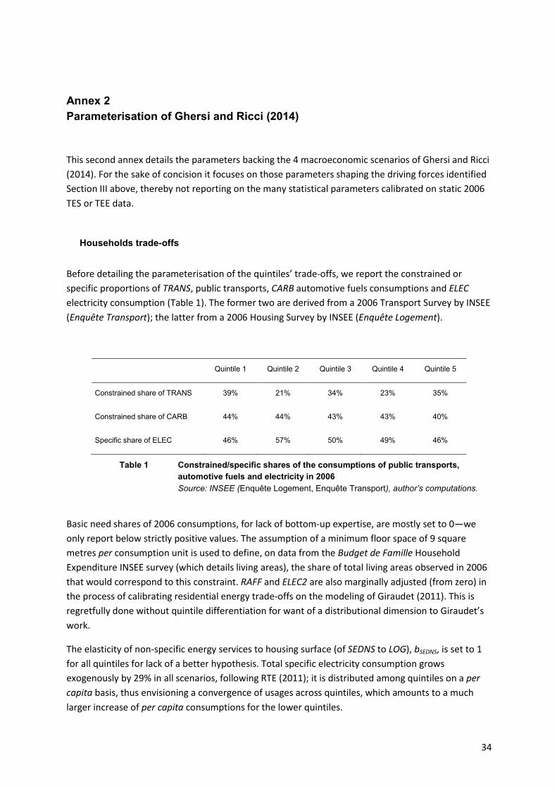
34
Annex 2
Parameterisation of Ghersi and Ricci (2014)
This second annex details the parameters backing the 4 macroeconomic scenarios of Ghersi and Ricci
(2014). For the sake of concision it focuses on those parameters shaping the driving forces identified
Section III above, thereby not reporting on the many statistical parameters calibrated on static 2006
TES or TEE data.
Households trade-offs
Before detailing the parameterisation of the quintiles’ trade-offs, we report the constrained or
specific proportions of TRANS, public transports, CARB automotive fuels consumptions and ELEC
electricity consumption (Table 1). The former two are derived from a 2006 Transport Survey by INSEE
(Enquête Transport); the latter from a 2006 Housing Survey by INSEE (Enquête Logement).
Quintile 1 Quintile 2 Quintile 3 Quintile 4 Quintile 5
Constrained share of TRANS 39% 21% 34% 23% 35%
Constrained share of CARB 44% 44% 43% 43% 40%
Specific share of ELEC 46% 57% 50% 49% 46%
Table 1 Constrained/specific shares of the consumptions of public transports,
automotive fuels and electricity in 2006
Source: INSEE (Enquête Logement, Enquête Transport), author’s computations.
Basic need shares of 2006 consumptions, for lack of bottom-up expertise, are mostly set to 0—we
only report below strictly positive values. The assumption of a minimum floor space of 9 square
metres per consumption unit is used to define, on data from the Budget de Famille Household
Expenditure INSEE survey (which details living areas), the share of total living areas observed in 2006
that would correspond to this constraint. RAFF and ELEC2 are also marginally adjusted (from zero) in
the process of calibrating residential energy trade-offs on the modeling of Giraudet (2011). This is
regretfully done without quintile differentiation for want of a distributional dimension to Giraudet’s
work.
The elasticity of non-specific energy services to housing surface (of SEDNS to LOG), bSEDNS, is set to 1
for all quintiles for lack of a better hypothesis. Total specific electricity consumption grows
exogenously by 29% in all scenarios, following RTE (2011); it is distributed among quintiles on a per
capita basis, thus envisioning a convergence of usages across quintiles, which amounts to a much
larger increase of per capita consumptions for the lower quintiles.
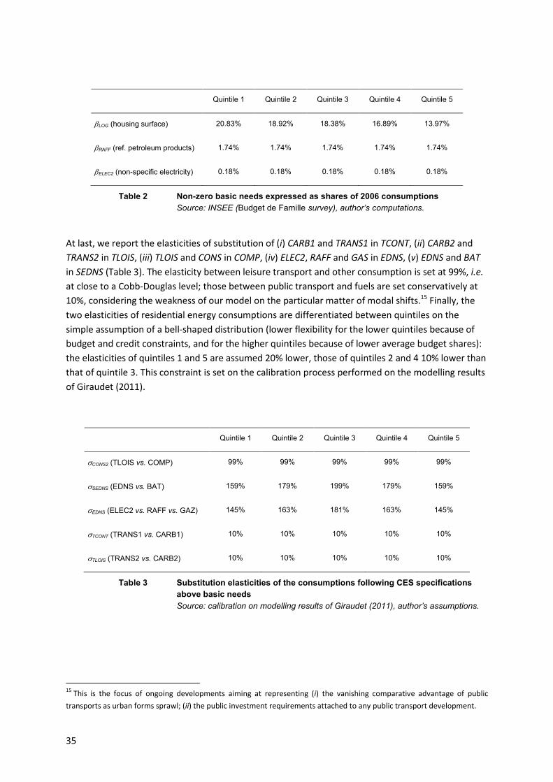
35
Quintile 1 Quintile 2 Quintile 3 Quintile 4 Quintile 5
LOG (housing surface) 20.83% 18.92% 18.38% 16.89% 13.97%
RAFF (ref. petroleum products) 1.74% 1.74% 1.74% 1.74% 1.74%
ELEC2 (non-specific electricity) 0.18% 0.18% 0.18% 0.18% 0.18%
Table 2 Non-zero basic needs expressed as shares of 2006 consumptions
Source: INSEE (Budget de Famille survey), author’s computations.
At last, we report the elasticities of substitution of (i) CARB1 and TRANS1 in TCONT, (ii) CARB2 and
TRANS2 in TLOIS, (iii) TLOIS and CONS in COMP, (iv) ELEC2, RAFF and GAS in EDNS, (v) EDNS and BAT
in SEDNS (Table 3). The elasticity between leisure transport and other consumption is set at 99%, i.e.
at close to a Cobb-Douglas level; those between public transport and fuels are set conservatively at
10%, considering the weakness of our model on the particular matter of modal shifts.15 Finally, the
two elasticities of residential energy consumptions are differentiated between quintiles on the
simple assumption of a bell-shaped distribution (lower flexibility for the lower quintiles because of
budget and credit constraints, and for the higher quintiles because of lower average budget shares):
the elasticities of quintiles 1 and 5 are assumed 20% lower, those of quintiles 2 and 4 10% lower than
that of quintile 3. This constraint is set on the calibration process performed on the modelling results
of Giraudet (2011).
Quintile 1 Quintile 2 Quintile 3 Quintile 4 Quintile 5
CONS2 (TLOIS vs. COMP) 99% 99% 99% 99% 99%
SEDNS (EDNS vs. BAT) 159% 179% 199% 179% 159%
EDNS (ELEC2 vs. RAFF vs. GAZ) 145% 163% 181% 163% 145%
TCONT (TRANS1 vs. CARB1) 10% 10% 10% 10% 10%
TLOIS (TRANS2 vs. CARB2) 10% 10% 10% 10% 10%
Table 3 Substitution elasticities of the consumptions following CES specifications
above basic needs
Source: calibration on modelling results of Giraudet (2011), author’s assumptions.
15
This is the focus of ongoing developments aiming at representing (i) the vanishing comparative advantage of public
transports as urban forms sprawl; (ii) the public investment requirements attached to any public transport development.

36
Firms’ trade-offs
Firms’ trade-offs regard the optimal balance of 11 inputs to production, i.e. 9 intermediate
consumptions (secondary factors), and the 2 primary factors of Labour and Capital. Considering its
focus on household behaviour, and the substantial increase of the number of goods disaggregated
from overall activity compared to previous versions (from 4 to 9 aggregate goods), the model
currently does not calibrate the behaviours of the production systems on dedicated techno-economic
expertise (cf. Hourcade and Ghersi, 2006).
Trade-offs between inputs in the 9 productions are thus represented in a standard way, through as
many CES-type functions, with a priori constant substitution elasticities. However, these CES forms
only partially apply to the 2006 input volumes: input-specific technical asymptotes are assumed, to
schematise the physical constraints weighing upon the evolution of production processes;
substitution elasticities are thus not constant, but rather decrease as input intensities approach their
asymptotes. This is arguably a necessary feature when considering trade-offs in technical systems,
including energy ones, at the middle- to long-term horizon of 29 years (2006 to 2035). Boonekamp
(2009) argues in favour of such a limitation to adaptive capacity in the case of households.
The floors to input intensities are generally set at conservative levels, tending to consider substantial
rigidities over the projected horizon—at least compared to standard CGEMs where they are implicitly
systematically nil.16 For intermediate consumptions they are deliberately set at higher levels when
the underlying consumptions are simultaneously quite explicit and presumably little flexible. One
example is the intensity in EPRIM (i.e. crude oil) of the production of CARB (automotive fuels): the
floor is set at 100%, which amounts to the Leontief assumption of a fixed intermediate consumption
coefficient in a context where EPRIM relative prices strongly increase.
The substitution elasticities between the tradable shares of each input are set at 120% for all
productions. For each input this value must be corrected by the share of their 2006 consumption
deemed adjustable to measure the effective substitution elasticity (measured over the entire
consumption and not only on its flexible share) to all other inputs. For example the elasticity of
substitution of labour to other inputs to the composite good production is 25% of 120%, that is 30%
only. This value furthermore only prevails at the 2006 equilibrium. The point elasticity of substitution
is indeed lower in any equilibrium where the labour intensity is lower than its 2006 value—indeed it
tends towards 0 as the labour intensity draws closer to its floor value, 25% below its 2006 level as far
as composite production is concerned.
16
The point-of-view of our comment could be turned around and the standard model underlined as envisaging extremely
weak rigidities.
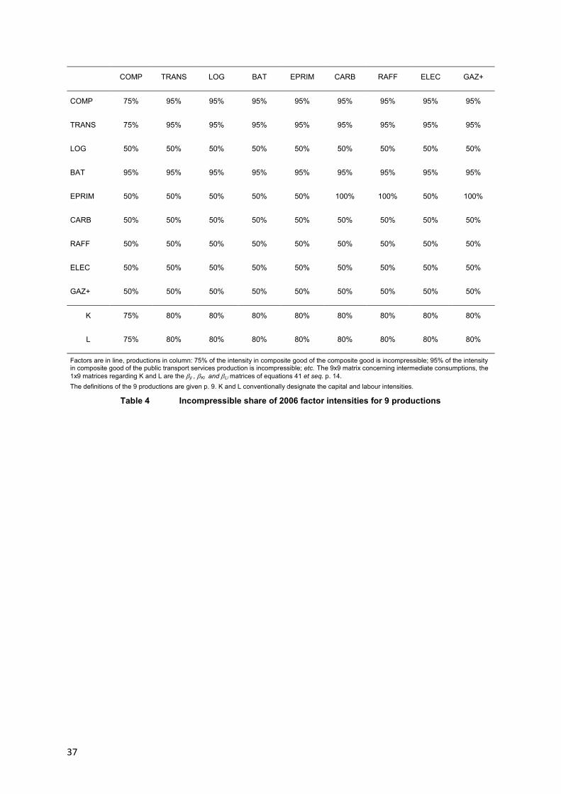
37
COMP TRANS LOG BAT EPRIM CARB RAFF ELEC GAZ+
COMP 75% 95% 95% 95% 95% 95% 95% 95% 95%
TRANS 75% 95% 95% 95% 95% 95% 95% 95% 95%
LOG 50% 50% 50% 50% 50% 50% 50% 50% 50%
BAT 95% 95% 95% 95% 95% 95% 95% 95% 95%
EPRIM 50% 50% 50% 50% 50% 100% 100% 50% 100%
CARB 50% 50% 50% 50% 50% 50% 50% 50% 50%
RAFF 50% 50% 50% 50% 50% 50% 50% 50% 50%
ELEC 50% 50% 50% 50% 50% 50% 50% 50% 50%
GAZ+ 50% 50% 50% 50% 50% 50% 50% 50% 50%
K 75% 80% 80% 80% 80% 80% 80% 80% 80%
L 75% 80% 80% 80% 80% 80% 80% 80% 80%
Factors are in line, productions in column: 75% of the intensity in composite good of the composite good is incompressible; 95% of the intensity in composite good of the public transport services production is incompressible; etc. The 9x9 matrix concerning intermediate consumptions, the 1x9 matrices regarding K and L are the ji , Ki and Li matrices of equations 41 et seq. p. 14.
The definitions of the 9 productions are given p. 9. K and L conventionally designate the capital and labour intensities.
Table 4 Incompressible share of 2006 factor intensities for 9 productions