© DIGITAL VISION

Digital Object Identifier 10.1109/MSP.2007.914731

Conventional approaches to sampling signals or images follow Shannon’s cel-ebrated theorem: the sampling rate must be at least twice the maximum fre-quency present in the signal (the so-called Nyquist rate). In fact, thisprinciple underlies nearly all signal acquisition protocols used in consumeraudio and visual electronics, medical imaging devices, radio receivers, and

so on. (For some signals, such as images that are not naturally bandlimited, the sam-pling rate is dictated not by the Shannon theorem but by the desired temporal or spatialresolution. However, it is common in such systems to use an antialiasing low-pass filterto bandlimit the signal before sampling, and so the Shannon theorem plays an implicitrole.) In the field of data conversion, for example, standard analog-to-digital converter(ADC) technology implements the usual quantized Shannon representation: the signal isuniformly sampled at or above the Nyquist rate.

[Emmanuel J. Candès

and Michael B. Wakin]

An Introduction ToCompressive Sampling

[A sensing/sampling paradigm that goes against the common knowledge in data acquisition]

1053-5888/08/$25.00©2008IEEE IEEE SIGNAL PROCESSING MAGAZINE [21] MARCH 2008

This article surveys the theory of compressive sampling, alsoknown as compressed sensing or CS, a novel sensing/samplingparadigm that goes against the common wisdom in data acquisi-tion. CS theory asserts that one can recover certain signals andimages from far fewer samples or measurements than tradition-al methods use. To make this possible, CS relies on two princi-ples: sparsity, which pertains to the signals of interest, andincoherence, which pertains to the sensing modality.

■ Sparsity expresses the idea that the “informationrate” of a continuous time signal may be much smallerthan suggested by its bandwidth, or that a discrete-timesignal depends on a number of degrees of freedomwhich is comparably much smaller than its (finite)length. More precisely, CS exploits the fact that manynatural signals are sparse or compressible in the sensethat they have concise rep-resentations when expressedin the proper basis � .■ Incoherence extends theduality between time and fre-quency and expresses the ideathat objects having a sparserepresentation in � must bespread out in the domain inwhich they are acquired, just as a Dirac or a spike in thetime domain is spread out in the frequency domain. Putdifferently, incoherence says that unlike the signal ofinterest, the sampling/sensing waveforms have anextremely dense representation in � .The crucial observation is that one can design efficient

sensing or sampling protocols that capture the useful infor-mation content embedded in a sparse signal and condense itinto a small amount of data. These protocols are nonadaptiveand simply require correlating the signal with a small num-ber of fixed waveforms that are incoherent with the sparsify-ing basis. What is most remarkable about these samplingprotocols is that they allow a sensor to very efficiently cap-ture the information in a sparse signal without trying tocomprehend that signal. Further, there is a way to usenumerical optimization to reconstruct the full-length signalfrom the small amount of collected data. In other words, CSis a very simple and efficient signal acquisition protocolwhich samples—in a signal independent fashion—at a lowrate and later uses computational power for reconstructionfrom what appears to be an incomplete set of measurements.

Our intent in this article is to overview the basic CS theorythat emerged in the works [1]–[3], present the key mathemat-ical ideas underlying this theory, and survey a couple ofimportant results in the field. Our goal is to explain CS asplainly as possible, and so our article is mainly of a tutorialnature. One of the charms of this theory is that it draws fromvarious subdisciplines within the applied mathematical sci-ences, most notably probability theory. In this review, we havedecided to highlight this aspect and especially the fact thatrandomness can—perhaps surprisingly—lead to very effective

sensing mechanisms. We will also discuss significant implica-tions, explain why CS is a concrete protocol for sensing andcompressing data simultaneously (thus the name), and con-clude our tour by reviewing important applications.

THE SENSING PROBLEMIn this article, we discuss sensing mechanisms in which infor-mation about a signal f (t) is obtained by linear functionalsrecording the values

yk = 〈 f, ϕk〉, k = 1, . . . , m. (1)

That is, we simply correlate the object we wish to acquirewith the waveforms ϕk(t). This is a standard setup. If thesensing waveforms are Dirac delta functions (spikes), for

example, then y is a vector ofsampled values of f in the timeor space domain. If the sensingwaveforms are indicator func-tions of pixels, then y is theimage data typically collected bysensors in a digital camera. If thesensing waveforms are sinusoids,then y is a vector of Fourier coef-

ficients; this is the sensing modality used in magnetic reso-nance imaging (MRI). Other examples abound.

Although one could develop a CS theory of continuoustime/space signals, we restrict our attention to discrete sig-nals f ∈ Rn. The reason is essentially twofold: first, this isconceptually simpler and second, the available discrete CStheory is far more developed (yet clearly paves the way for acontinuous theory—see also “Applications”). Having saidthis, we are then interested in undersampled situations inwhich the number m of available measurements is muchsmaller than the dimension n of the signal f . Such problemsare extremely common for a variety of reasons. For instance,the number of sensors may be limited. Or the measurementsmay be extremely expensive as in certain imaging processesvia neutron scattering. Or the sensing process may be slowso that one can only measure the object a few times as inMRI. And so on.

These circumstances raise important questions. Isaccurate reconstruction possible from m � n measure-ments only? Is it possible to design m � n sensing wave-forms to capture almost all the information about f ? Andhow can one approximate f from this information?Admittedly, this state of affairs looks rather daunting, asone would need to solve an underdetermined linear systemof equations. Letting A denote the m × n sensing matrixwith the vectors ϕ∗

1 , . . . , ϕ∗m as rows (a∗ is the complex

transpose of a), the process of recovering f ∈ Rn fromy = Af ∈ Rm is ill-posed in general when m < n: there areinfinitely many candidate signals f̃ for which Af̃ = y. Butone could perhaps imagine a way out by relying on realis-tic models of objects f which naturally exist. The Shannon

CS THEORY ASSERTS THAT ONE CANRECOVER CERTAIN SIGNALS AND

IMAGES FROM FAR FEWER SAMPLESOR MEASUREMENTS THAN

TRADITIONAL METHODS USE.

IEEE SIGNAL PROCESSING MAGAZINE [22] MARCH 2008

theory tells us that, if f(t) actually has very low band-width, then a small number of (uniform) samples will suf-fice for recovery. As we will see in the remainder of thisarticle, signal recovery can actually be made possible for amuch broader class of signal models.

INCOHERENCE AND THE SENSING OF SPARSE SIGNALSThis section presents the two fundamental premises underlyingCS: sparsity and incoherence.

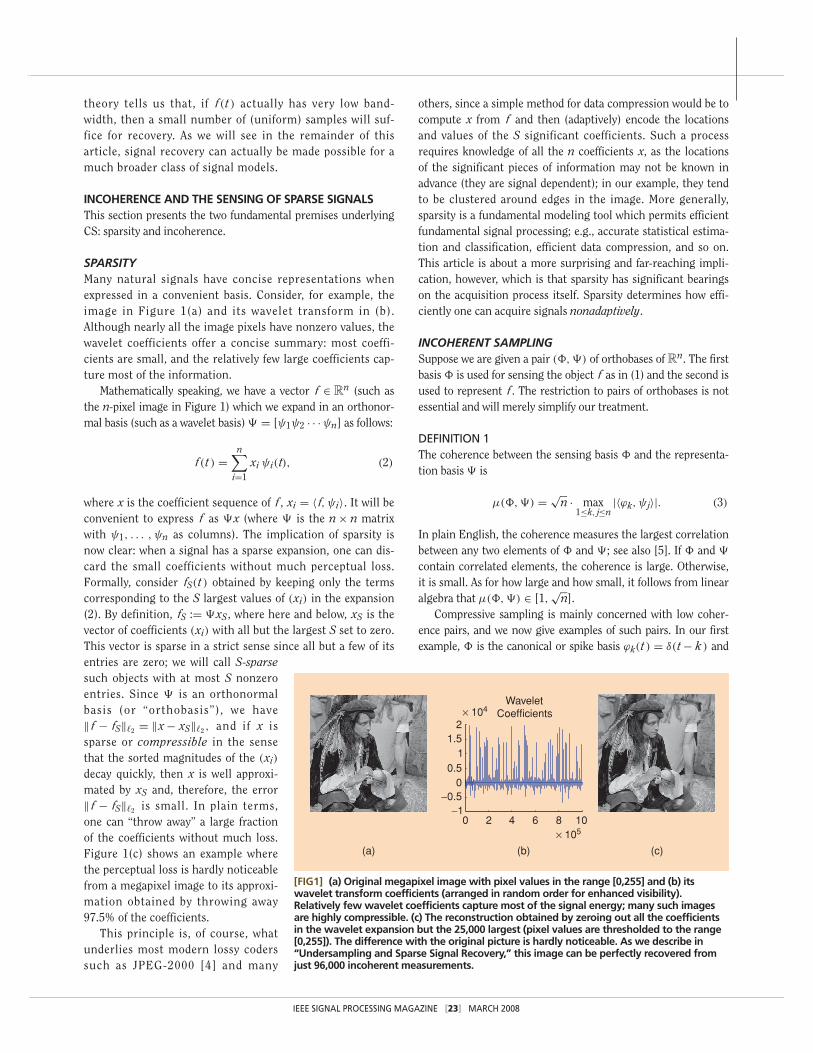
SPARSITYMany natural signals have concise representations whenexpressed in a convenient basis. Consider, for example, theimage in Figure 1(a) and its wavelet transform in (b).Although nearly all the image pixels have nonzero values, thewavelet coefficients offer a concise summary: most coeffi-cients are small, and the relatively few large coefficients cap-ture most of the information.

Mathematically speaking, we have a vector f ∈ Rn (such asthe n-pixel image in Figure 1) which we expand in an orthonor-mal basis (such as a wavelet basis) � = [ψ1ψ2 · · ·ψn] as follows:

f(t) =n∑

i=1

xi ψi(t), (2)

where x is the coefficient sequence of f , xi = 〈 f, ψi〉. It will beconvenient to express f as �x (where � is the n × n matrixwith ψ1, . . . , ψn as columns). The implication of sparsity isnow clear: when a signal has a sparse expansion, one can dis-card the small coefficients without much perceptual loss.Formally, consider fS(t) obtained by keeping only the termscorresponding to the S largest values of (xi) in the expansion(2). By definition, fS := �xS, where here and below, xS is thevector of coefficients (xi) with all but the largest S set to zero.This vector is sparse in a strict sense since all but a few of itsentries are zero; we will call S-sparsesuch objects with at most S nonzeroentries. Since � is an orthonormalbasis (or “orthobasis”), we have‖ f − fS‖�2 = ‖x − xS‖�2 , and if x issparse or compressible in the sensethat the sorted magnitudes of the (xi)

decay quickly, then x is well approxi-mated by xS and, therefore, the error‖ f − fS‖�2 is small. In plain terms,one can “throw away” a large fractionof the coefficients without much loss.Figure 1(c) shows an example wherethe perceptual loss is hardly noticeablefrom a megapixel image to its approxi-mation obtained by throwing away97.5% of the coefficients.

This principle is, of course, whatunderlies most modern lossy coderssuch as JPEG-2000 [4] and many

others, since a simple method for data compression would be tocompute x from f and then (adaptively) encode the locationsand values of the S significant coefficients. Such a processrequires knowledge of all the n coefficients x, as the locationsof the significant pieces of information may not be known inadvance (they are signal dependent); in our example, they tendto be clustered around edges in the image. More generally,sparsity is a fundamental modeling tool which permits efficientfundamental signal processing; e.g., accurate statistical estima-tion and classification, efficient data compression, and so on.This article is about a more surprising and far-reaching impli-cation, however, which is that sparsity has significant bearingson the acquisition process itself. Sparsity determines how effi-ciently one can acquire signals nonadaptively.

INCOHERENT SAMPLINGSuppose we are given a pair (�,�) of orthobases of Rn. The firstbasis � is used for sensing the object f as in (1) and the second isused to represent f . The restriction to pairs of orthobases is notessential and will merely simplify our treatment.

DEFINITION 1The coherence between the sensing basis � and the representa-tion basis � is

μ(�,�) = √n · max

1≤k, j≤n|〈ϕk, ψ j〉|. (3)

In plain English, the coherence measures the largest correlationbetween any two elements of � and �; see also [5]. If � and �contain correlated elements, the coherence is large. Otherwise,it is small. As for how large and how small, it follows from linearalgebra that μ(�,�) ∈ [1,

√n].

Compressive sampling is mainly concerned with low coher-ence pairs, and we now give examples of such pairs. In our firstexample, � is the canonical or spike basis ϕk(t) = δ(t − k ) and

[FIG1] (a) Original megapixel image with pixel values in the range [0,255] and (b) itswavelet transform coefficients (arranged in random order for enhanced visibility).Relatively few wavelet coefficients capture most of the signal energy; many such imagesare highly compressible. (c) The reconstruction obtained by zeroing out all the coefficientsin the wavelet expansion but the 25,000 largest (pixel values are thresholded to the range[0,255]). The difference with the original picture is hardly noticeable. As we describe in“Undersampling and Sparse Signal Recovery,” this image can be perfectly recovered fromjust 96,000 incoherent measurements.

(a) (b)

−10 2 4 6 8 10

−0.50

0.5

1.52

WaveletCoefficients× 104

1

(c)

× 105

IEEE SIGNAL PROCESSING MAGAZINE [23] MARCH 2008

� is the Fourier basis, ψ j (t) = n−1/ 2 e i 2π jt/n. Since � is thesensing matrix, this corresponds to the classical sampling schemein time or space. The time-frequency pair obeys μ(�,�) = 1and, therefore, we have maximalincoherence. Further, spikes andsinusoids are maximally incoherentnot just in one dimension but inany dimension, (in two dimensions,three dimensions, etc.)

Our second example takeswavelets bases for � and noiselets[6] for �. The coherence betweennoiselets and Haar wavelets is

√2 and that between noiselets and

Daubechies D4 and D8 wavelets is, respectively, about 2.2 and 2.9across a wide range of sample sizes n. This extends to higherdimensions as well. (Noiselets are also maximally incoherent withspikes and incoherent with the Fourier basis.) Our interest innoiselets comes from the fact that 1) they are incoherent with sys-tems providing sparse representations of image data and othertypes of data, and 2) they come with very fast algorithms; thenoiselet transform runs in O(n) time, and just like the Fouriertransform, the noiselet matrix does not need to be stored to beapplied to a vector. This is of crucial practical importance fornumerically efficient CS implementations.

Finally, random matrices are largely incoherent with anyfixed basis � . Select an orthobasis � uniformly at random,which can be done by orthonormalizing n vectors sampledindependently and uniformly on the unit sphere. Then withhigh probability, the coherence between � and � is about√

2 log n. By extension, random waveforms (ϕk (t)) with inde-pendent identically distributed (i.i.d.) entries, e.g., Gaussianor ±1 binary entries, will also exhibit a very low coherencewith any fixed representation �. Note the rather strangeimplication here; if sensing with incoherent systems is good,then efficient mechanisms ought to acquire correlations withrandom waveforms, e.g., white noise!

UNDERSAMPLING AND SPARSE SIGNAL RECOVERYIdeally, we would like to measure all the n coefficients of f , butwe only get to observe a subset of these and collect the data

yk = 〈 f, ϕk〉, k ∈ M, (4)

where M ⊂ {1, . . . , n} is a subset of cardinality m < n. Withthis information, we decide to recover the signal by �1-normminimization; the proposed reconstruction f � is given byf � = �x�, where x� is the solution to the convex optimizationprogram (‖x‖�1 := ∑

i |xi|)

minx̃∈Rn

‖x̃‖�1 subject to yk = 〈ϕk,� x̃ 〉, ∀ k ∈ M. (5)

That is, among all objects f̃ = � x̃ consistent with the data, wepick that whose coefficient sequence has minimal �1 norm. (Asis well known, minimizing �1 subject to linear equality con-

straints can easily be recast as a linear program making avail-able a host of ever more efficient solution algorithms.)

The use of the �1 norm as a sparsity-promoting functiontraces back several decades. Aleading early application wasreflection seismology, in which asparse reflection function (indi-cating meaningful changesbetween subsurface layers) wassought from bandlimited data[7], [8]. However, �1-minimiza-tion is not the only way to

recover sparse solutions; other methods, such as greedyalgorithms [9], have also been proposed.

Our first result asserts that when f is sufficiently sparse, therecovery via �1-minimization is provably exact.

THEOREM 1 [10]Fix f ∈ Rn and suppose that the coefficient sequence x of f inthe basis � is S-sparse. Select m measurements in the �domain uniformly at random. Then if

m ≥ C · μ2(�,�) · S · log n (6)

for some positive constant C, the solution to (5) is exact withoverwhelming probability. (It is shown that the probability ofsuccess exceeds 1 − δ if m ≥ C · μ2(�,�) · S · log(n/δ) . Inaddition, the result is only guaranteed for nearly all signsequences x with a fixed support, see [10] for details.)

We wish to make three comments: 1) The role of the coherence is completely transparent;the smaller the coherence, the fewer samples are needed,hence our emphasis on low coherence systems in theprevious section.2) One suffers no information loss by measuring justabout any set of m coefficients which may be far less thanthe signal size apparently demands. If μ(�,�) is equal orclose to one, then on the order of S log n samples sufficeinstead of n. 3) The signal f can be exactly recovered from our con-densed data set by minimizing a convex functional whichdoes not assume any knowledge about the number ofnonzero coordinates of x, their locations, or their ampli-tudes which we assume are all completely unknown a pri-ori. We just run the algorithm and if the signal happens tobe sufficiently sparse, exact recovery occurs.The theorem indeed suggests a very concrete acquisition

protocol: sample nonadaptively in an incoherent domain andinvoke linear programming after the acquisition step. Followingthis protocol would essentially acquire the signal in a com-pressed form. All that is needed is a decoder to “decompress”this data; this is the role of �1 minimization.

In truth, this random incoherent sampling theorem extendsan earlier result about the sampling of spectrally sparse signals[1], which showed that randomness 1) can be a very effective

MANY NATURAL SIGNALS ARESPARSE OR COMPRESSIBLE IN THESENSE THAT THEY HAVE CONCISE

REPRESENTATIONS WHENEXPRESSED IN THE PROPER BASIS.

IEEE SIGNAL PROCESSING MAGAZINE [24] MARCH 2008

sensing mechanism and 2) is amenable to rigorous proofs, andthus perhaps triggered the many CS developments we have wit-nessed and continue to witness today. Suppose that we areinterested in sampling ultra-wideband but spectrally sparse sig-nals of the form f(t) = ∑n−1

j=0 xj e i 2 π j t/ n, t = 0, . . . , n − 1,

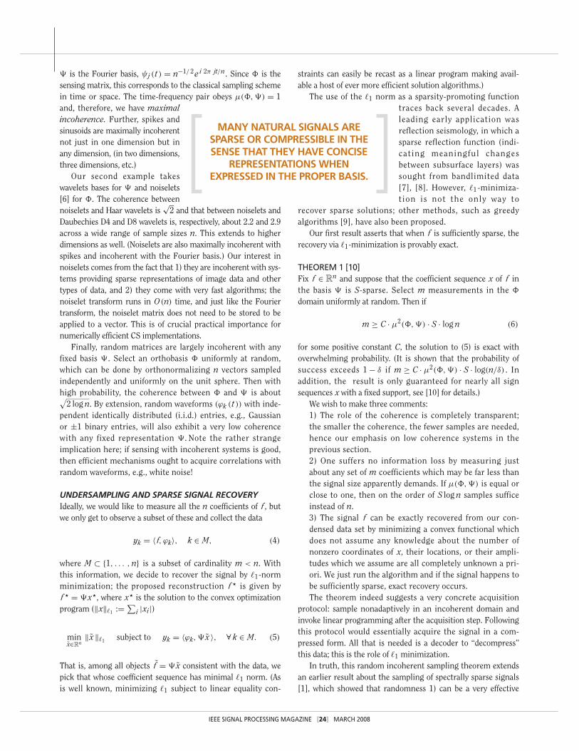
where n is very large but where the number of nonzero compo-nents xj is less than or equal to S (which we should think of ascomparably small). We do not know which frequencies areactive nor do we know the amplitudes on this active set.Because the active set is not necessarily a subset of consecutiveintegers, the Nyquist/Shannon theory is mostly unhelpful(since one cannot restrict the bandwidth a priori, one may beled to believe that all n time samples are needed). In this specialinstance, Theorem 1 claims that one can reconstruct a signalwith arbitrary and unknown frequency support of size S fromon the order of S log n time samples, see [1]. What is more,these samples do not have to be carefully chosen; almost anysample set of this size will work. An illustrative example is pro-vided in Figure 2. For other types of theoretical results in thisdirection using completely different ideas see [11]–[13].

It is now time to discuss the role played by probability in allof this. The key point is that to get useful and powerful results,one needs to resort to a probabilistic statement since one can-not hope for comparable results holding for all measurementsets of size m. Here is why. There are special sparse signalsthat vanish nearly everywhere in the � domain. In otherwords, one can find sparse signals f and very large subsets ofsize almost n (e.g., n − S ) for which yk = 〈 f, ϕk〉 = 0 for allk ∈ M. The interested reader may want to check the exampleof the Dirac comb discussed in [14] and [1]. On the one hand,given such subsets, one would get to see a stream of zeros andno algorithm whatsoever would of course be able reconstructthe signal. On the other hand, the theorem guarantees that thefraction of sets for which exact recovery does not occur is trulynegligible (a large negative power of n). Thus, we only have totolerate a probability of failure that is extremely small. Forpractical purposes, the probability of failure is zero providedthat the sampling size is sufficiently large.

Interestingly, the study of special sparse signals discussedabove also shows that one needs at least on the order ofμ2 · S · log n samples as well. (We are well aware that thereexist subsets of cardinality 2S in the time domain which canreconstruct any S-sparse signal in the frequency domain.Simply take 2S consecutive time points, see “What IsComprehensive Sampling?” and [11] and [12], for example.But this is not what our claim is about. We want that mostsets of a certain size provide exact reconstruction.) With fewersamples, the probability that information may be lost is justtoo high and reconstruction by any method, no matter howintractable, is impossible. In summary, when the coherence isone, say, we do not need more than S log n samples but wecannot do with fewer either.

We conclude this section with an incoherent sampling exam-ple, and consider the sparse image in Figure 1(c), which as werecall has only 25,000 nonzero wavelet coefficients. We then

[FIG2] (a) A sparse real valued signal and (b) its reconstructionfrom 60 (complex valued) Fourier coefficients by �1minimization. The reconstruction is exact. (c) The minimumenergy reconstruction obtained by substituting the �1 normwith the �2 norm; �1 and �2 give wildly different answers. The�2 solution does not provide a reasonable approximation tothe original signal.

(a)

0 200 400 600−2

−1

0

1

2

0 200 400 600−2

−1

0

1

2

0 200 400 600−2

−1

0

1

2

Sparse Signal

Original

(b)

(c)

Original

Original

Recovered

Recovered

l2 Recovery

l1 recovery

IEEE SIGNAL PROCESSING MAGAZINE [25] MARCH 2008

acquire information by taking 96,000 incoherent measurements(see [10] for the particulars of these measurements) and solve (5).The minimum-�1 recovery is per-fect; that is, f � = f . This exampleshows that a number of samplesjust about 4× the sparsity level suf-fices. Many researchers havereported on similar empirical suc-cesses. There is de facto a knownfour-to-one practical rule whichsays that for exact recovery, oneneeds about four incoherent sam-ples per unknown nonzero term.

ROBUST COMPRESSIVE SAMPLINGWe have shown that one could recover sparse signals from just afew measurements but in order to be really powerful, CS needsto be able to deal with both nearly sparse signals and with noise.First, general objects of interest are not exactly sparse butapproximately sparse. The issue here is whether or not it is pos-sible to obtain accurate reconstructions of such objects fromhighly undersampled measurements. Second, in any real appli-cation measured data will invariably be corrupted by at least asmall amount of noise as sensing devices do not have infiniteprecision. It is therefore imperative that CS be robust vis a vissuch nonidealities. At the very least, small perturbations in thedata should cause small perturbations in the reconstruction.

This section examines these two issues simultaneously.Before we begin, however, it will ease the exposition to considerthe abstract problem of recovering a vector x ∈ Rn from data

y = Ax + z, (7)

where A is an m × n “sensing matrix” giving us information aboutx, and z is a stochastic or deterministic unknown error term. Thesetup of the last section is of this form since with f = �x andy = R�f (R is the m × n matrix extracting the sampled coordi-nates in M), one can write y = Ax, where A = R��. Hence, onecan work with the abstract model (7) bearing in mind that x maybe the coefficient sequence of the object in a proper basis.

RESTRICTED ISOMETRIESIn this section, we introduce a key notion that has proved to bevery useful to study the general robustness of CS; the so-calledrestricted isometry property (RIP) [15].

DEFINITION 2For each integer S = 1, 2, . . . , define the isometry constant δS

of a matrix A as the smallest number such that

(1 − δS)‖x‖2�2

≤ ‖Ax‖2�2

≤ (1 + δS)‖x‖2�2

(8)

holds for all S-sparse vectors x.We will loosely say that a matrix A obeys the RIP of order S if

δS is not too close to one. When this property holds, A approxi-

mately preserves the Euclidean length of S-sparse signals, whichin turn implies that S-sparse vectors cannot be in the null space

of A. (This is useful as otherwisethere would be no hope of recon-structing these vectors.) An equiv-alent description of the RIP is tosay that all subsets of S columnstaken from A are in fact nearlyorthogonal (the columns of A can-not be exactly orthogonal since wehave more columns than rows).

To see the connection betweenthe RIP and CS, imagine we wishto acquire S-sparse signals with

A. Suppose that δ2S is sufficiently less than one. This impliesthat all pairwise distances between S-sparse signals must bewell preserved in the measurement space. That is,(1 − δ2S)‖x1 − x2‖2

�2≤ ‖Ax1 − Ax2‖2

�2≤ (1 + δ2S)‖x1− x2 |2�2

holds for all S-sparse vectors x1, x2. As demonstrated in thenext section, this encouraging fact guarantees the existenceof efficient and robust algorithms for discriminating S-sparsesignals based on their compressive measurements.

GENERAL SIGNAL RECOVERYFROM UNDERSAMPLED DATAIf the RIP holds, then the following linear program gives anaccurate reconstruction:

minx̃∈Rn

‖x̃‖�1 subject to Ax̃ = y (= Ax). (9)

THEOREM 2 [16]Assume that δ2S <

√2 − 1. Then the solution x� to (9) obeys

‖x� − x‖�2 ≤ C0 · ‖x − xS‖�1/√

S and

‖x� − x‖�1 ≤ C0 · ‖x − xS‖�1 (10)

for some constant C0, where xS is the vector x with all butthe largest S components set to 0. (As stated, this result isdue to the first author [17] and yet unpublished, see also [16]and [18].)

The conclusions of Theorem 2 are stronger than those ofTheorem 1. If x is S-sparse, then x = xS and, thus, the recov-ery is exact. But this new theorem deals with all signals. If xis not S-sparse, then (10) asserts that the quality of therecovered signal is as good as if one knew ahead of time thelocation of the S largest values of x and decided to measurethose directly. In other words, the reconstruction is nearly asgood as that provided by an oracle which, with full and per-fect knowledge about x, extracts the S most significant piecesof information for us.

Another striking difference with our earlier result is that itis deterministic; it involves no probability. If we are fortunateenough to hold a sensing matrix A obeying the hypothesis of

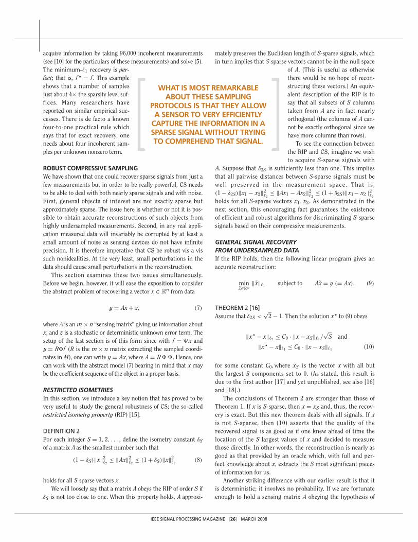
WHAT IS MOST REMARKABLEABOUT THESE SAMPLING

PROTOCOLS IS THAT THEY ALLOWA SENSOR TO VERY EFFICIENTLY

CAPTURE THE INFORMATION IN ASPARSE SIGNAL WITHOUT TRYINGTO COMPREHEND THAT SIGNAL.

IEEE SIGNAL PROCESSING MAGAZINE [26] MARCH 2008

the theorem, we may apply it, and we are then guaranteed torecover all sparse S-vectors exactly, and essentially the S-largest entries of all vectors otherwise; i.e., there is no proba-bility of failure.

What is missing at this point is the relationship between S(the number of components one can effectively recover) obey-ing the hypothesis and m the number of measurements orrows of the matrix. To derive powerful results, we would liketo find matrices obeying the RIP with values of S close to m.Can one design such matrices? In the next section, we willshow that this is possible, but first we examine the robustnessof CS vis a vis data corruption.

ROBUST SIGNAL RECOVERY FROM NOISY DATAWe are given noisy data as in (7) and use �1 minimization withrelaxed constraints for reconstruction:

min ‖x̃‖�1 subject to ‖Ax̃ − y‖�2 ≤ ε, (11)

where ε bounds the amount of noise in the data. (One couldalso consider recovery programs such as the Dantzig selector[19] or a combinatorial optimization program proposed byHaupt and Nowak [20]; both algorithms have provable resultsin the case where the noise is Gaussian with bounded vari-ance.) Problem (11) is often called the LASSO after [21]; seealso [22]. To the best of our knowledge, it was first proposed in[8]. This is again a convex problem (a second-order cone pro-gram) and can be solved efficiently.

THEOREM 3 [16]Assume that δ2S <

√2 − 1. Then the solution x� to (11) obeys

‖x� − x‖�2 ≤ C0 · ‖x − xS‖�1/√

S + C1 · ε (12)

for some constants C0 and C1. (Again, this theorem is unpub-lished as stated and is a variation on the result found in [16].)

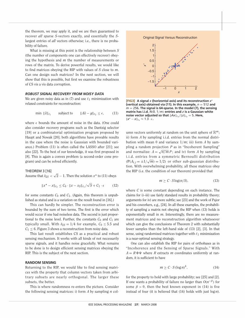
This can hardly be simpler. The reconstruction error isbounded by the sum of two terms. The first is the error whichwould occur if one had noiseless data. The second is just propor-tional to the noise level. Further, the constants C0 and C1 aretypically small. With δ2S = 1/4 for example, C0 ≤ 5.5 andC1 ≤ 6. Figure 3 shows a reconstruction from noisy data.

This last result establishes CS as a practical and robustsensing mechanism. It works with all kinds of not necessarilysparse signals, and it handles noise gracefully. What remainsto be done is to design efficient sensing matrices obeying theRIP. This is the subject of the next section.

RANDOM SENSINGReturning to the RIP, we would like to find sensing matri-ces with the property that column vectors taken from arbi-trary subsets are nearly orthogonal. The larger thesesubsets, the better.

This is where randomness re-enters the picture. Considerthe following sensing matrices: i) form A by sampling n col-

umn vectors uniformly at random on the unit sphere of Rm;ii) form A by sampling i.i.d. entries from the normal distri-bution with mean 0 and variance 1/m; iii) form A by sam-pling a random projection P as in “Incoherent Sampling”and normalize: A = √

n/m P ; and iv) form A by samplingi.i.d. entries from a symmetric Bernoulli distribution(P(Ai, j = ±1/

√m) = 1/2) or other sub-gaussian distribu-

tion. With overwhelming probability, all these matrices obeythe RIP (i.e. the condition of our theorem) provided that

m ≥ C · S log(n/S), (13)

where C is some constant depending on each instance. Theclaims for i)–iii) use fairly standard results in probability theory;arguments for iv) are more subtle; see [23] and the work of Pajorand his coworkers, e.g., [24]. In all these examples, the probabili-ty of sampling a matrix not obeying the RIP when (13) holds isexponentially small in m. Interestingly, there are no measure-ment matrices and no reconstruction algorithm whatsoeverwhich can give the conclusions of Theorem 2 with substantiallyfewer samples than the left-hand side of (13) [2], [3]. In thatsense, using randomized matrices together with �1 minimizationis a near-optimal sensing strategy.

One can also establish the RIP for pairs of orthobases as in“Incoherence and the Sensing of Sparse Signals.” WithA = R�� where R extracts m coordinates uniformly at ran-dom, it is sufficient to have

m ≥ C · S (log n)4, (14)

for the property to hold with large probability; see [25] and [2].If one wants a probability of failure no larger than O(n−β) forsome β > 0, then the best known exponent in (14) is fiveinstead of four (it is believed that (14) holds with just log n).

[FIG3] A signal x (horizontal axis) and its reconstruction x�

(vertical axis) obtained via (11). In this example, n = 512 andm = 256. The signal is 64-sparse. In the model (7), the sensingmatrix has i.i.d. N(0, 1/m) entries and z is a Gaussian whitenoise vector adjusted so that ‖Ax‖�2/‖z‖�2 = 5. Here,‖x� − x‖�2 ≈ 1.3 · ε.

−1 0 1 2

−1.5

−1

−0.5

0

0.5

1

1.5

2

Original Signal Versus Reconstruction

x

x∗

IEEE SIGNAL PROCESSING MAGAZINE [27] MARCH 2008

This proves that one can stably and accurately reconstructnearly sparse signals from dramatically undersampled data inan incoherent domain.

Finally, the RIP can also hold for sensing matrices A = ��,where � is an arbitrary orthobasis and � is an m × n measure-ment matrix drawn randomly from a suitable distribution. If onefixes � and populates � as in i)–iv), then with overwhelming prob-ability, the matrix A = �� obeysthe RIP provided that (13) is satis-fied, where again C is some con-stant depending on each instance.These random measurement matri-ces � are in a sense universal [23];the sparsity basis need not even beknown when designing the meas-urement system!

WHAT IS COMPRESSIVE SAMPLING?Data acquisition typically works as follows: massive amounts ofdata are collected only to be—in large part—discarded at thecompression stage to facilitate storage and transmission. In thelanguage of this article, one acquires a high-resolution pixel arrayf , computes the complete set of transform coefficients, encodethe largest coefficients and discard all the others, essentially end-ing up with fS. This process of massive data acquisition followedby compression is extremely wasteful (one can think about a digi-tal camera which has millions of imaging sensors, the pixels, buteventually encodes the picture in just a few hundred kilobytes).

CS operates very differently, and performs as “if it were possi-ble to directly acquire just the important information about theobject of interest.” By taking about O(S log(n/S)) random projec-tions as in “Random Sensing,” one has enough information toreconstruct the signal with accuracy at least as good as that pro-vided by fS, the best S-term approximation—the best compressedrepresentation—of the object. In other words, CS measurementprotocols essentially translate analog data into an already com-pressed digital form so that one can—at least in principle—obtainsuper-resolved signals from just a few sensors. All that is neededafter the acquisition step is to “decompress” the measured data.

There are some superficial similarities between CS andideas in coding theory and more precisely with the theory andpractice of Reed-Solomon (RS) codes [26]. In a nutshell andin the context of this article, it is well known that one canadapt ideas from coding theory to establish the following: onecan uniquely reconstruct any S-sparse signal from the data ofits first 2S Fourier coefficients, yk = ∑n−1

t=0 xt e−i 2π kt/n,

k = 0, 1, 2, . . . , 2S − 1, or from any set of 2S consecutive fre-quencies for that matter (the computational cost for therecovery is essentially that of solving an S × S Toeplitz systemand of taking an n-point fast Fourier transform). Does thismean that one can use this technique to sense compressiblesignals? The answer is negative and there are two main rea-sons for this. First, the problem is that RS decoding is analgebraic technique, which cannot deal with nonsparse sig-nals (the decoding finds the support by rooting a polynomial);

second, the problem of finding the support of a signal—evenwhen the signal is exactly sparse—from its first 2S Fouriercoefficients is extraordinarily ill posed (the problem is thesame as that of extrapolating a high degree polynomial from asmall number of highly clustered values). Tiny perturbationsof these coefficients will give completely different answers sothat with finite precision data, reliable estimation of the sup-

port is practically impossible.Whereas purely algebraic meth-ods ignore the conditioning ofinformation operators, havingwell-conditioned matrices, whichare crucial for accurate estima-tion, is a central concern in CS asevidenced by the role played bythe RIP.

APPLICATIONSThe fact that a compressible signal can be captured effi-ciently using a number of incoherent measurements that isproportional to its information level S � n has implicationsthat are far reaching and concern a number of possibleapplications:

■ Data compression. In some situations, the sparse basis �may be unknown at the encoder or impractical to implementfor data compression. As we discussed in “Random Sensing,”however, a randomly designed � can be considered a universalencoding strategy, as it need not be designed with regards tothe structure of �. (The knowledge and ability to implement� are required only for the decoding or recovery of f .) Thisuniversality may be particularly helpful for distributed sourcecoding in multi-signal settings such as sensor networks [27].We refer the reader to articles by Haupt et al. and Goyal et al.elsewhere in this issue for related discussions.■ Channel coding. As explained in [15], CS principles (spar-sity, randomness, and convex optimization) can be turnedaround and applied to design fast error correcting codes overthe reals to protect from errors during transmission.■ Inverse problems. In still other situations, the only way toacquire f may be to use a measurement system � of a cer-tain modality. However, assuming a sparse basis � exists forf that is also incoherent with �, then efficient sensing willbe possible. One such application involves MR angiography[1] and other types of MR setups [28], where � records asubset of the Fourier transform, and the desired image f issparse in the time or wavelet domains. Elsewhere in thisissue, Lustig et al. discuss this application in more depth.■ Data acquisition. Finally, in some important situations thefull collection of n discrete-time samples of an analog signalmay be difficult to obtain (and possibly difficult to subse-quently compress). Here, it could be helpful to design physi-cal sampling devices that directly record discrete, low-rateincoherent measurements of the incident analog signal.The last of these applications suggests that mathematical

and computational methods could have an enormous impact

IEEE SIGNAL PROCESSING MAGAZINE [28] MARCH 2008

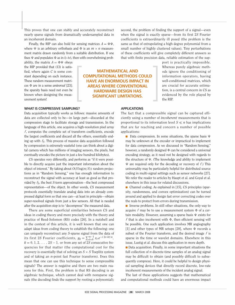
MATHEMATICAL ANDCOMPUTATIONAL METHODS COULD

HAVE AN ENORMOUS IMPACT INAREAS WHERE CONVENTIONAL

HARDWARE DESIGN HASSIGNIFICANT LIMITATIONS.

IEEE SIGNAL PROCESSING MAGAZINE [29] MARCH 2008

in areas where conventional hardware design has significantlimitations. For example, conventional imaging devices thatuse CCD or CMOS technology are limited essentially to thevisible spectrum. However, a CS camera that collects incoher-ent measurements using a digital micromirror array (andrequires just one photosensitive element instead of millions)could significantly expand thesecapabilities. (See [29] and an arti-cle by Duarte et al. in this issue.)

Along these same lines, partof our research has focused onadvancing devices for “analog-to-information” (A/I) conversionof high-bandwidth signals (seealso the article by Healy et al. inthis issue). Our goal is to helpalleviate the pressure on conventional ADC technology,which is currently limited to sample rates on the order of 1GHz. As an alternative, we have proposed two specific archi-tectures for A/I in which a discrete, low-rate sequence ofincoherent measurements can be acquired from a high-bandwidth analog signal. To a high degree of approxima-tion, each measurement yk can be interpreted as the innerproduct 〈 f, ϕk〉 of the incident analog signal f against ananalog measurement waveform ϕk. As in the discrete CSframework, our preliminary results suggest that analog sig-nals obeying a sparse or compressible model (in some ana-log dictionary � ) can be captured efficiently using thesedevices at a rate proportional to their information levelinstead of their Nyquist rate. Of course, there are challengesone must address when applying the discrete CS methodol-ogy to the recovery of sparse analog signals. A thoroughtreatment of these issues would be beyond the scope of thisshort article and as a first cut, one might simply accept theidea that in many cases, discretizing/sampling the sparsedictionary allows for suitable recovery. Our two architec-tures are as follows:

1) Nonuniform Sampler (NUS). Our first architecture simplydigitizes the signal at randomly or pseudo-randomly sampledtime points. That is, yk = f(tk) = 〈 f, δtk〉. In effect, these

time points are obtained by jittering nominal (low-rate)sample points located on a regular lattice. Due to the inco-herence between spikes and sines, this architecture can beused to sample signals having sparse frequency spectra farbelow their Nyquist rate. There are of course tremendousbenefits associated with a reduced sampling rate, as this

provides added circuit settlingtime and has the effect of reduc-ing the noise level.2) Random Modulation Prein-tegration (RMPI). Our secondarchitecture is applicable to awider variety of sparsity domains,most notably those signals hav-ing a sparse signature in thetime-frequency plane. Whereas it

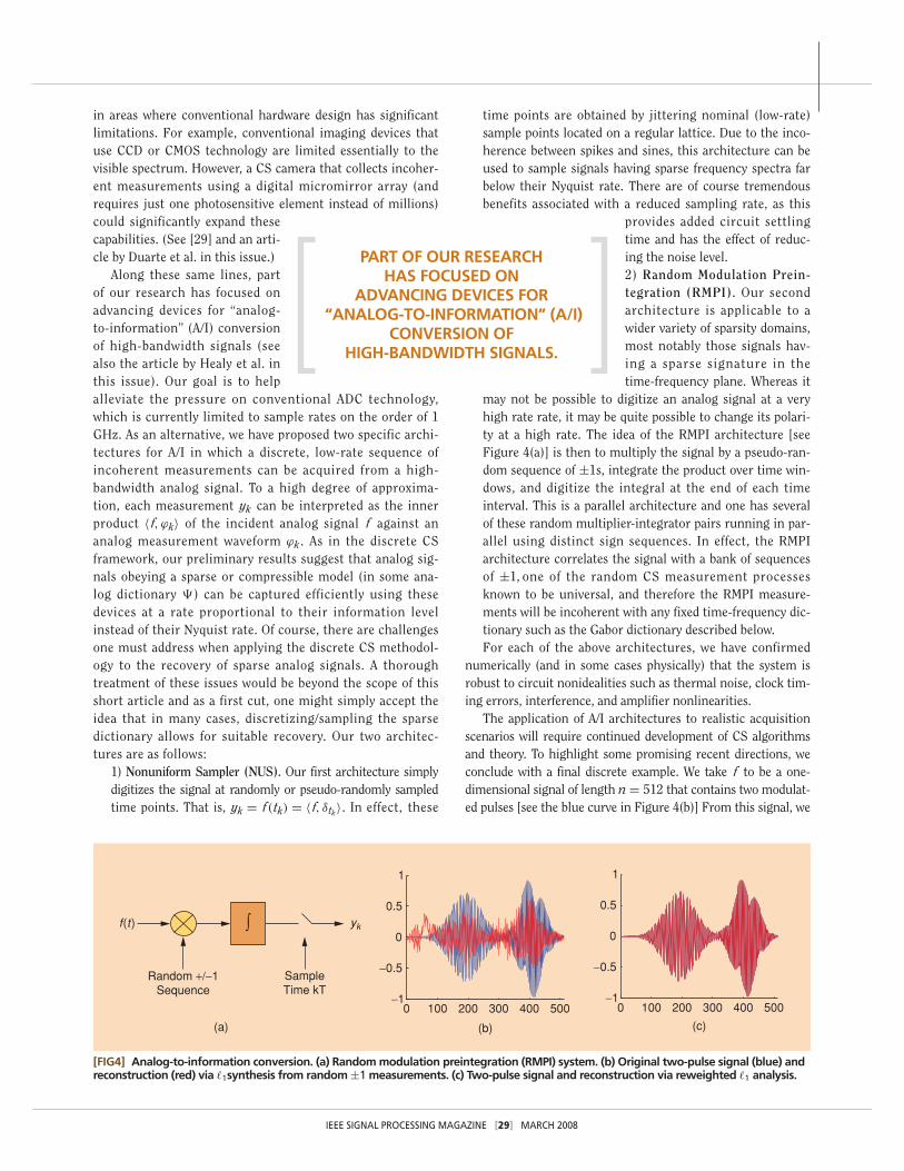
may not be possible to digitize an analog signal at a veryhigh rate rate, it may be quite possible to change its polari-ty at a high rate. The idea of the RMPI architecture [seeFigure 4(a)] is then to multiply the signal by a pseudo-ran-dom sequence of ±1s, integrate the product over time win-dows, and digitize the integral at the end of each timeinterval. This is a parallel architecture and one has severalof these random multiplier-integrator pairs running in par-allel using distinct sign sequences. In effect, the RMPIarchitecture correlates the signal with a bank of sequencesof ±1, one of the random CS measurement processesknown to be universal, and therefore the RMPI measure-ments will be incoherent with any fixed time-frequency dic-tionary such as the Gabor dictionary described below.For each of the above architectures, we have confirmed

numerically (and in some cases physically) that the system isrobust to circuit nonidealities such as thermal noise, clock tim-ing errors, interference, and amplifier nonlinearities.

The application of A/I architectures to realistic acquisitionscenarios will require continued development of CS algorithmsand theory. To highlight some promising recent directions, weconclude with a final discrete example. We take f to be a one-dimensional signal of length n = 512 that contains two modulat-ed pulses [see the blue curve in Figure 4(b)] From this signal, we

[FIG4] Analog-to-information conversion. (a) Random modulation preintegration (RMPI) system. (b) Original two-pulse signal (blue) andreconstruction (red) via �1synthesis from random ±1 measurements. (c) Two-pulse signal and reconstruction via reweighted �1 analysis.

(a) (b)

0 100 200 300 400 500−1

−0.5

0

0.5

1

(c)

0 100 200 300 400 500−1

−0.5

0

0.5

1

∫f(t) yk

Random +/−1Sequence

SampleTime kT

PART OF OUR RESEARCH HAS FOCUSED ON

ADVANCING DEVICES FOR“ANALOG-TO-INFORMATION” (A/I)

CONVERSION OF HIGH-BANDWIDTH SIGNALS.

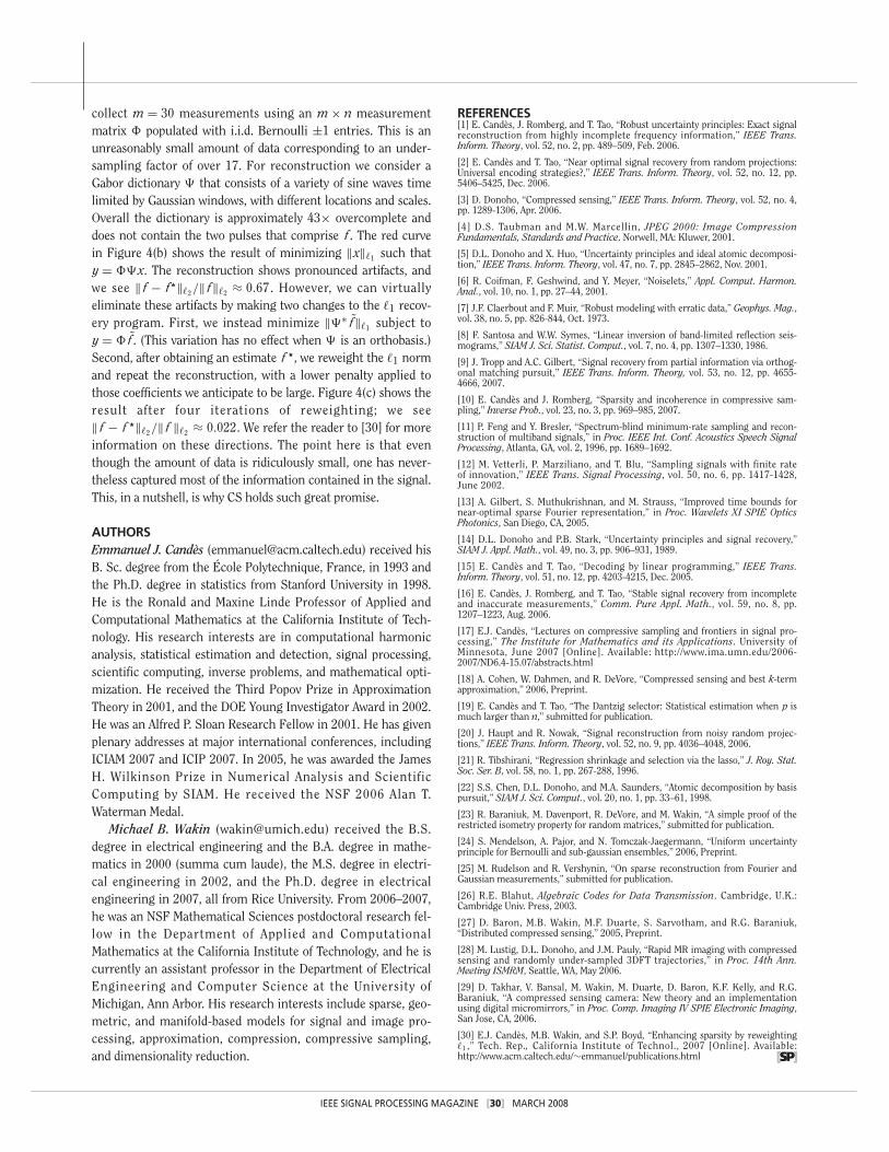
collect m = 30 measurements using an m × n measurementmatrix � populated with i.i.d. Bernoulli ±1 entries. This is anunreasonably small amount of data corresponding to an under-sampling factor of over 17. For reconstruction we consider aGabor dictionary � that consists of a variety of sine waves timelimited by Gaussian windows, with different locations and scales.Overall the dictionary is approximately 43× overcomplete anddoes not contain the two pulses that comprise f . The red curvein Figure 4(b) shows the result of minimizing ‖x‖�1 such thaty = ��x. The reconstruction shows pronounced artifacts, andwe see ‖ f − f�‖�2/‖ f‖�2 ≈ 0.67. However, we can virtuallyeliminate these artifacts by making two changes to the �1 recov-ery program. First, we instead minimize ‖�∗ f̃‖�1 subject toy = � f̃ . (This variation has no effect when � is an orthobasis.)Second, after obtaining an estimate f �, we reweight the �1 normand repeat the reconstruction, with a lower penalty applied tothose coefficients we anticipate to be large. Figure 4(c) shows theresult after four iterations of reweighting; we see‖ f − f �‖�2/‖ f ‖�2 ≈ 0.022. We refer the reader to [30] for moreinformation on these directions. The point here is that eventhough the amount of data is ridiculously small, one has never-theless captured most of the information contained in the signal.This, in a nutshell, is why CS holds such great promise.

AUTHORSEmmanuel J. Candès (emmanuel@acm.caltech.edu) received hisB. Sc. degree from the École Polytechnique, France, in 1993 andthe Ph.D. degree in statistics from Stanford University in 1998.He is the Ronald and Maxine Linde Professor of Applied andComputational Mathematics at the California Institute of Tech-nology. His research interests are in computational harmonicanalysis, statistical estimation and detection, signal processing,scientific computing, inverse problems, and mathematical opti-mization. He received the Third Popov Prize in ApproximationTheory in 2001, and the DOE Young Investigator Award in 2002.He was an Alfred P. Sloan Research Fellow in 2001. He has givenplenary addresses at major international conferences, includingICIAM 2007 and ICIP 2007. In 2005, he was awarded the JamesH. Wilkinson Prize in Numerical Analysis and ScientificComputing by SIAM. He received the NSF 2006 Alan T.Waterman Medal.

Michael B. Wakin (wakin@umich.edu) received the B.S.degree in electrical engineering and the B.A. degree in mathe-matics in 2000 (summa cum laude), the M.S. degree in electri-cal engineering in 2002, and the Ph.D. degree in electricalengineering in 2007, all from Rice University. From 2006–2007,he was an NSF Mathematical Sciences postdoctoral research fel-low in the Department of Applied and ComputationalMathematics at the California Institute of Technology, and he iscurrently an assistant professor in the Department of ElectricalEngineering and Computer Science at the University ofMichigan, Ann Arbor. His research interests include sparse, geo-metric, and manifold-based models for signal and image pro-cessing, approximation, compression, compressive sampling,and dimensionality reduction.

REFERENCES[1] E. Candès, J. Romberg, and T. Tao, “Robust uncertainty principles: Exact signalreconstruction from highly incomplete frequency information,” IEEE Trans.Inform. Theory, vol. 52, no. 2, pp. 489–509, Feb. 2006.

[2] E. Candès and T. Tao, “Near optimal signal recovery from random projections:Universal encoding strategies?,” IEEE Trans. Inform. Theory, vol. 52, no. 12, pp.5406–5425, Dec. 2006.

[3] D. Donoho, “Compressed sensing,” IEEE Trans. Inform. Theory, vol. 52, no. 4,pp. 1289-1306, Apr. 2006.

[4] D.S. Taubman and M.W. Marcellin, JPEG 2000: Image CompressionFundamentals, Standards and Practice. Norwell, MA: Kluwer, 2001.

[5] D.L. Donoho and X. Huo, “Uncertainty principles and ideal atomic decomposi-tion,” IEEE Trans. Inform. Theory, vol. 47, no. 7, pp. 2845–2862, Nov. 2001.

[6] R. Coifman, F. Geshwind, and Y. Meyer, “Noiselets,” Appl. Comput. Harmon.Anal., vol. 10, no. 1, pp. 27–44, 2001.

[7] J.F. Claerbout and F. Muir, “Robust modeling with erratic data,” Geophys. Mag.,vol. 38, no. 5, pp. 826-844, Oct. 1973.

[8] F. Santosa and W.W. Symes, “Linear inversion of band-limited reflection seis-mograms,” SIAM J. Sci. Statist. Comput., vol. 7, no. 4, pp. 1307–1330, 1986.

[9] J. Tropp and A.C. Gilbert, “Signal recovery from partial information via orthog-onal matching pursuit,” IEEE Trans. Inform. Theory, vol. 53, no. 12, pp. 4655-4666, 2007.

[10] E. Candès and J. Romberg, “Sparsity and incoherence in compressive sam-pling,” Inverse Prob., vol. 23, no. 3, pp. 969–985, 2007.

[11] P. Feng and Y. Bresler, “Spectrum-blind minimum-rate sampling and recon-struction of multiband signals,” in Proc. IEEE Int. Conf. Acoustics Speech SignalProcessing, Atlanta, GA, vol. 2, 1996, pp. 1689–1692.

[12] M. Vetterli, P. Marziliano, and T. Blu, “Sampling signals with finite rateof innovation,” IEEE Trans. Signal Processing, vol. 50, no. 6, pp. 1417-1428,June 2002.

[13] A. Gilbert, S. Muthukrishnan, and M. Strauss, “Improved time bounds fornear-optimal sparse Fourier representation,” in Proc. Wavelets XI SPIE OpticsPhotonics, San Diego, CA, 2005.

[14] D.L. Donoho and P.B. Stark, “Uncertainty principles and signal recovery,”SIAM J. Appl. Math., vol. 49, no. 3, pp. 906–931, 1989.

[15] E. Candès and T. Tao, “Decoding by linear programming,” IEEE Trans.Inform. Theory, vol. 51, no. 12, pp. 4203-4215, Dec. 2005.

[16] E. Candès, J. Romberg, and T. Tao, “Stable signal recovery from incompleteand inaccurate measurements,” Comm. Pure Appl. Math., vol. 59, no. 8, pp.1207–1223, Aug. 2006.

[17] E.J. Candès, “Lectures on compressive sampling and frontiers in signal pro-cessing,” The Institute for Mathematics and its Applications. University ofMinnesota, June 2007 [Online]. Available: http://www.ima.umn.edu/2006-2007/ND6.4-15.07/abstracts.html

[18] A. Cohen, W. Dahmen, and R. DeVore, “Compressed sensing and best k-termapproximation,” 2006, Preprint.

[19] E. Candès and T. Tao, “The Dantzig selector: Statistical estimation when p ismuch larger than n,” submitted for publication.

[20] J. Haupt and R. Nowak, “Signal reconstruction from noisy random projec-tions,” IEEE Trans. Inform. Theory, vol. 52, no. 9, pp. 4036–4048, 2006.

[21] R. Tibshirani, “Regression shrinkage and selection via the lasso,” J. Roy. Stat.Soc. Ser. B, vol. 58, no. 1, pp. 267-288, 1996.

[22] S.S. Chen, D.L. Donoho, and M.A. Saunders, “Atomic decomposition by basispursuit,” SIAM J. Sci. Comput., vol. 20, no. 1, pp. 33–61, 1998.

[23] R. Baraniuk, M. Davenport, R. DeVore, and M. Wakin, “A simple proof of therestricted isometry property for random matrices,” submitted for publication.

[24] S. Mendelson, A. Pajor, and N. Tomczak-Jaegermann, “Uniform uncertaintyprinciple for Bernoulli and sub-gaussian ensembles,” 2006, Preprint.

[25] M. Rudelson and R. Vershynin, “On sparse reconstruction from Fourier andGaussian measurements,” submitted for publication.

[26] R.E. Blahut, Algebraic Codes for Data Transmission. Cambridge, U.K.:Cambridge Univ. Press, 2003.

[27] D. Baron, M.B. Wakin, M.F. Duarte, S. Sarvotham, and R.G. Baraniuk,“Distributed compressed sensing,” 2005, Preprint.

[28] M. Lustig, D.L. Donoho, and J.M. Pauly, “Rapid MR imaging with compressedsensing and randomly under-sampled 3DFT trajectories,” in Proc. 14th Ann.Meeting ISMRM, Seattle, WA, May 2006.

[29] D. Takhar, V. Bansal, M. Wakin, M. Duarte, D. Baron, K.F. Kelly, and R.G.Baraniuk, “A compressed sensing camera: New theory and an implementationusing digital micromirrors,” in Proc. Comp. Imaging IV SPIE Electronic Imaging,San Jose, CA, 2006.

[30] E.J. Candès, M.B. Wakin, and S.P. Boyd, “Enhancing sparsity by reweighting�1 ,” Tech. Rep., California Institute of Technol., 2007 [Online]. Available:http://www.acm.caltech.edu/∼emmanuel/publications.html [SP]

IEEE SIGNAL PROCESSING MAGAZINE [30] MARCH 2008