Control and Cybernetics

vol. XX (XXXX) No. XRevisiting the Analysis of Optimal Control Problems withSeveral State Constraints1byJ. Frédéri Bonnans1 and Audrey Hermant21 INRIA-Sa lay and CMAP, E ole Polyte hnique, 91128 Palaiseau, Fran e.2 Centre d'Analyse de Défense, DGA, 16 bis avenue Prieur de la C�te d'Or,94114 Ar ueil, Fran e.Abstra t: This paper improves the results and gives shorterproofs for the analysis of state onstrained optimal ontrol problemspresented by the authors in Bonnans and Hermant (2009b), on- erning se ond order optimality onditions and the well-posedness ofthe shooting algorithm. The hypothesis for the se ond order ne es-sary onditions is weaker, and the main results are obtained withoutredu tion to the normal form used in that referen e, and withoutanalysis of high order regularity results for the ontrol. In addition,we provide some numeri al illustration. The essential tool is the useof the �alternative optimality system�.Keywords: Optimal ontrol, state onstraints, shhoting algo-rithm, se ond order optimality onditions.1. Introdu tionIn these notes we give an a ount of some re ent results on the analysis ofstate- onstrained optimal ontrol problems (see the lassi al review by Hartl,Sethi, and Vi kson (1995)) using in an essential way the approa h alled �alter-native optimality system�. This approa h was introdu ed in an informal way byBryson, Denham and Dreyfus (1963), Ja obson, Lele and Speyer (1971). Thebasi idea is, when a state onstraint is a tive over an interval of time, to re-pla e it with its time derivative of smallest order su h that the ontrol appears.Adding in a proper way jun tion onditions, it is then possible to state a shoot-ing algorithm. Maurer (1979) gave a sound mathemati al basis to this approa hby de�ning in a pre ise way the alternative ostate, and giving the alternativeformulation of the optimality onditions, but restri ting the analysis mainly to(important) spe ial ases su h as a single ontrol and onstraint. So many im-portant questions remained open for a long time, su h as the jun tion analysis1The authors thank the two referees for their useful omments.

2 J.F. Bonnans and A. Hermantin the general ase, se ond order optimality onditions, and the well-posednessof numeri al algorithms, among them the shooting algorithm.There are a number of re ent paper devoted to state- onstrained problems,see Malanowski (2007) and referen es theirein, Malanowski and Maurer (2001).An appli ation to the omputation of onstrained spline fun tions is dis ussedin Opfer and Oberle (1988). Let us highlight Malanowski and Maurer (1998)where a omplete theory is obtained for �rst order state onstraints. High order onstraints were studied in Bonnans and Hermant (2007-2009) and Hermant(2008,2009a,2009b). In this paper we revisit the problem studied in Bonnansand Hermant (2009b), by improving some results and simplifying some of theproofs. Part of the simpli� ation is due to the fa t that we are able to obtain themain results without using the redu tion to the normal form (see Bonnans andHermant (2009b)) and also without analysing high order regularity results forthe ontrol. Other important points are se ond-order ne essary optimality on-ditions with weaker hypotheses than in Bonnans and Hermant (2007,2009b), thesimpli� ation of the presentation of jun tion ondition for the alternative ostateand linearized ostate (and its relation to the jump of the standard ostate) anda detailed analysis of the di�eren e of osts of the asso iated quadrati subprob-lems. This last point is related to the fa t, that a jun tion point for a given onstraint auses jumps in the multipliers of the other a tive onstraints. Thisis why the ase of several state onstraints is essentially more di� ult than the ase of a single one, dis ussed in many papers. We provide also a more om-pa t and self- ontained presentation of the results. The analysis allows for state onstraints of order higher than two. However, the analysis of the shooting al-gorithm ex ludes boundary ar s with su h onstraints, as expe ted (see remark3). The paper is organized as follows. Se tion 2 dis usses some onsequen es ofPontryagin's prin iple and provides some results on the ontinuity of the ontrol.For the latter we rely on the fa t that the ontrol minimizes the Hamiltonian. Inthis se tion we establish high order regularity on ar s with onstant a tive set of onstraints. The shooting algorithm (and related questions on se ond-order op-timality onditions) is presented in se tion 3, using redu tion of isolated onta tpoints and the alternative optimality system. Se ond-order optimality ondi-tions are presented in se tion 4. The well-posedness of the shooting algorithm isestablished in se tion 5, assuming in parti ular that no boundary ar has state onstraint of order higher than two. In se tion 6, we present a numeri al ap-pli ation of the shooting algorithm on two a ademi s problems involving threestate onstraints of order 1 and 2, respe tively.Notations The set of integers from i to j is denoted {i:j}. The operator � :=�means a de�nition of the l.h.s. The ardinal of a set I is denoted by |I|. Theopen (resp. losed) Eu lidean ball of enter x and radiusR is denoted by B(x, R)(resp. B(x, R)).For the value of fun tions of time only, as say y, we denote yt the value

Optimal Control Problems with Several State Constraints 3at time t and the one of its ith omponent is denoted yi,t. If u and y dependon time, and h is a fun tion of (t, u, y), we denote by hi,y(t, ut, yt) the partialderivative w.r.t y of its ith omponent. When ne essary for larity we denotepartial derivatives say like Dth(t, ut, yt).The Sobolev spa e Wm,s(0, T, IRn), where m is a positive integer and s ∈[1,∞], is the set of fun tions in Ls(0, T, IRn) whose weak time derivatives alsobelong to Ls(0, T, IRn). Elements of W 1,s(0, T, IRn) are Hölder (resp. Lips hitz)fun tions of time for s ∈ [1,∞) (resp. s = ∞).The spa e of fun tions of [0, T ] → IRn with bounded variations is denotedBV (0, T, IRn). The measure asso iated with η ∈ BV (0, T ) is denoted dη. El-ements of BV (0, T, IRn) have for all time t ∈ [0, T ], left and right limits (rightlimit for t = 0, left limit for t = T ). If a fun tion of time say η has left or rightlimits at time t, the latter are denoted η−

t and η+t , resp. The onvex ombina-tions of the latter are denoted ησ

t := ση+t + (1 − σ)η−

t , for σ ∈ [0, 1], and thejump at time t of η is [ηt] := η+t − η−

t .By IRn∗ we denote the dual of IRn, identi�ed with the spa e of n dimensionalhorizontal ve tors.2. Pontryagin's prin iple2.1. StatementIn this se tion we study optimal ontrol problems with state onstraints, of thefollowing type:

Min

∫ T

0

ℓ(ut, yt)dt + φ(yT );

yt = f(ut, yt); t ∈ (0, T ); y0 = y0;g(yt) ≤ 0; t ∈ [0, T ],

(1)with ℓ : IRm × IRn → IR, f : IRm × IRn → IRn, g : IRn → IRr, r ≥ 1, y0 ∈ IRngiven. All data f , g, ℓ, φ are of lass C∞, and f is Lips hitz. Denote the ontroland state spa es byU := L∞(0, T, IRm); Y := W 1,∞(0, T, IRn). (2)For a given u ∈ U , the state equation (i.e., the di�erential equation in these ond row of (1)) has a unique solution y(u) ∈ Y. The generalized Hamiltonianfun tion H : IR × IRm × IRn × IRn∗ → IR isH(α, u, y, p) := α ℓ(u, y) + pf(u, y). (3)Definition 1 We say that (u, y) ∈ U ×Y is a generalized Pontryagin extremalif there exists α ≥ 0 and η ∈ BV (0, T, IRr), with (α, dη) 6= 0, and a ostate

4 J.F. Bonnans and A. Hermantp ∈ BV (0, T, IRn∗), su h that a.e. t ∈ (0, T ):

˙yt = f(ut, yt) a.e. in [0, T ], (4)−dpt = Hy(α, ut, yt, pt)dt +

r∑

i=1

g′i(yt)dηi,t on [0, T ], (5)ut ∈ argmin

wH(α, w, yt, pt), a.a. on ]0, T [, (6)and in addition

gi(yt) ≤ 0; dηi,t ≥ 0; t ∈ [0, T ];

∫ T

0

gi(yt)dηi,t = 0, i ∈ {1 : r}, (7)y(0) = y0; pT = αφ′(yT ). (8)We an rewrite the ostate equation (5), with �nal ondition in (8), in integralform:

pt = αφ′(yt)+

∫ T

t

Hy(α, us, ys, ps)ds+

r∑

i=1

∫ T

t

g′i(ys)dηi,s, for all t ∈ [0, T ]. (9)The following is well-known, see Se tion 5.2 in Io�e (1979).Theorem 1 Let u ∈ U be an optimal ontrol and y be the asso iated state forproblem (1). Then (u, y) is a generalized Pontryagin extremal.2.2. Continuity of the ontrolThe total derivative of a fun tion of the state, say g(y), is by the de�nition thefun tion IRm × IRn → IRr whose expression isg(1)(u, y) := g′(y)f(u, y). (10)Along a traje tory (u, y) (i.e., a solution of the state equation), g(1)(ut, yt) isequal to d

dtg(yt). In a similar way we an de�ne higher order derivatives. Theseformal expressions are the sum of all partial derivatives multiplied by the or-responding derivative of the variable, understood as formal variables (and nottrue time derivatives) ex ept for y whose derivative is repla ed by f(u, y). De-noting the partial derivatives by subs ripts, we obtain for instan e the mapping

IRm × IRm × IRn → IRr

g(2)(u, u, y) = g(1)u (u, y)u + g(1)

y (u, y)f(u, y). (11)As long as the total derivatives do no depend on u (resp. the derivatives of u),we may denote them as g(i)(y) (resp. g(i)(u, y)).

Optimal Control Problems with Several State Constraints 5Definition 2 (i) For i ∈ {1 : r}, the order of the state onstraint gi(y) is thesmallest positive integer qi su h thatg(k)i,u (u, y) = 0, for all (u, y) ∈ IRm × IRn and 0 ≤ k < qi. (12)Then g(k)i (u, y) does not depend on the derivatives of u for k ≤ qi.(ii) We say that the state onstraint i is regular along a traje tory (u, y) ∈ U×Y,su h that u is ontinuous, if g

(qi)i,u (ut, yt) 6= 0, for all t ∈ [0, T ].For a state onstraint gi of order qi, and k ∈ {1 : (qi − 1)}, we may write

g(k)i (y) instead of g

(k)i (u, y), and we have

g(k+1)i (u, y) = g

(k)i,y (y)f(u, y); g

(k+1)i,u (u, y) = g

(k)i,y (y)fu(u, y). (13)For instan e, if qi ≥ 2, then skipping arguments of g and f :

{

g(2)i (u, y) = g

(1)i,y f = g′′i (f, f) + g′ifyf ;

g(2)i,u (u, y) = g

(1)i,y fu = (g′′i f + g′ify) fu.

(14)The set I(t) of a tive state onstraints at time t ∈ [0, T ] is de�ned byI(t) := {i ∈ {1 : r}; gi(y(t)) = 0}. (15)De�ne the set of state onstraints of order κ, and those a tive at time t alongthe traje tory (u, y) by:Iκ := {1 ≤ i ≤ r; qi = κ}; Iκ(t) := {i ∈ Iκ; gi(yt) = 0}. (16)For ontrol variables with left and right limits at every time, a strong Legendre-Clebs h type ondition, along the dire tion of jump of the ontrol, is as follows:{ For some α > 0: α|[ut]|

2 ≤ Huu(uσt , yt, p

σt )([ut], [ut]),for all σ ∈ [0, 1], t ∈ [0, T ].

(17)If the ontrol is ontinuous, the hypothesis of linear independen e w.r.t. the ontrol of �rst-order state onstraints is as follows:{g

(1)i,u(ut, yt)}i∈I1(t) is of rank |I1(t)|, for all t ∈ [0, T ]. (18)We re all that, being of bounded variation, p has left and right limits.Theorem 2 Let (u, y) be a Pontryagin extremal for problem (P ).(i) Let R > ‖u‖∞. If H(·, yt, p

±t ) has, for all t ∈ [0, T ], a unique minimum over

B(0, R), and if (17) holds, then u is ontinuous.(ii) If u is ontinuous and (18) hold, then the omponents of η asso iated with�rst order state onstraint are ontinuous, and Huu(ut, yt, pt±) is a ontinuousfun tion of time.

6 J.F. Bonnans and A. HermantProof. (i) By assumption, H(u, yt, p±t ) has a unique point of minimum at time

t at the point ut ∈ B(0, R). Then u = u a.e. and we may take u = u. Whensay t ↑ τ , ut has at least one luster point a. It is easy to he k that H(·, yt, p−t )attains its minimum on B(0, R) at the point a, implying the existen e of leftand right limits for u at time τ . By the ostate equation (5), p has at most ountably many jumps, of type

[pt] = p+t − p−t = −

r∑

i=1

νig′i(yt), with νi := [ηi,t] ≥ 0. (19)We have that

0 = Hu(u+t , yt, p

+t ) − Hu(u−

t , yt, p−t )

=

∫ 1

0

(Huu(uσt , yt, p

σt )[ut] + [pt]fu(uσ

t , yt)) dσ.(20)Using (19) and observing that g′ifu = g

(1)i,u = 0 if qi > 1, we obtain that

∫ 1

0

Huu(uσt , yt, p

σt )[ut]dσ =

∑

i∈I1

∫ 1

0

νig(1)i,u (uσ

t , yt)dσ. (21)Taking the s alar produ t of both sides of (21) by [ut], we get using hypothesis(17) thatα|[ut]|

2 ≤∑

i∈I1

∫ 1

0

νig(1)i,u(uσ, yt)[ut]dσ =

∑

i∈I1

νi

[

g(1)i (ut, yt)

]

. (22)If νi > 0, then gi(yt) = 0, and hen e [g(1)i (ut, yt)] ≤ 0 sin e t is a lo al maxi-mum of gi(yt). Therefore, the right-hand side in (22) is nonpositive, implying

[ut] = 0. Point (i) follows.(ii) Sin e [ut] = 0, the right-hand side of (21) (with uσt = ut) is zero. We on lude with (18) that the omponents of η asso iated with �rst order state onstraint are ontinuous. In addition, as g′i(y)fu(y, u) is identi ally zero when-ever qi > 1, it follows that Huu(ut, yt, pt±) is a ontinuous fun tion of time.Remark 1 We note that theorem 2 improves related statements in Bonnansand Hermant (2009b) and Maurer (1979) by using a weak hypothesis (17). Inthe sequel, if (u, y) is a Pontryagin extremal and u is ontinuous, we will saythat (u, y) is a ontinuous Pontryagin extremal (this of ourse does not implythe ontinuity of the multiplier η or of the ostate p).2.3. Smoothness on ea h ar If 0 ≤ a < b ≤ T , we say that (a, b) is an ar of the Pontryagin extremal

(u, y, p, η) if (a, b) is a maximal interval of [0, T ] over whi h the set of a tive

Optimal Control Problems with Several State Constraints 7 onstraints I(t) is onstant. Let qi be the order of the ith state onstraint, setq := (q1, . . . , qr), and de�ne G(u, y) : IRm × IRn → IRr by

Gi(u, y) := g(qi)i (u, y), i ∈ {1 : r}. (23)The hypothesis of linear independen e of gradients of a tive onstraints w.r.t.the ontrol is

{Gi,u(ut, yt)}i∈I(t) is of full rank, for all t ∈ [0, T ]. (24)We also need a strong Legendre-Clebs h ondition along the kernel of a tive onstraints:{ For some α > 0, for all t ∈ [0, T ], v ∈ IRm :

α|v|2 ≤ Huu(ut, yt, pt)(v, v), if Gi,u(ut, yt)v = 0, for all i ∈ I(t).(25)We introdu e like in Maurer (1979) the alternative multipliers ηi,k, where i ∈

{1 : r} and k ∈ {1 : qi}, and ηq:ηi,1

t := −ηi,t; ηi,kt :=

∫ T

t

ηi,k−1s ds; ηq

i := ηi,qi . (26)The alternative ostate (of order q) is de�ned aspq

t := pt −

r∑

i=1

qi∑

j=1

ηi,jt g

(j−1)i,y (yt) (27)and the orresponding alternative Hamiltonian Hq : IRm × IRn × IRn∗ × IRr∗ is

Hq(u, y, pq, ηq) := ℓ(u, y) + pqf(u, y) + ηqG(u, y). (28)This derivation of the alternative multipliers and the following proposition aredue to Maurer (1979):− ˙pq

t = Hqy(ut, yt, p

q, ηq), t ∈ (0, T ). (29)H(u, yt, pt) = Hq(u, yt, p

q, ηq), for all u ∈ IRm. (30)Proposition 1 Let (u, y, p, η) be a ontinuous Pontryagin extremal satisfying(24)-(25). Then u and ηq are of lass C∞ over any ar (and therefore so are ptand ηt).Proof. Let us denote by I∗ the set of a tive onstraints over an ar (a, b), andlet GI∗(u, y) := (Gi(u, y))i∈I∗ . The two algebrai equations{

Hqu(ut, yt, p

qt , η

qt ) = 0,

GI∗(ut, yt) = 0,(31)

8 J.F. Bonnans and A. Hermantare equal to zero over (a, b), and their Ja obian w.r.t. the algebrai variables(u, ηq) is

JacI(t) :=

(

Huu(ut, yt, pt) (GI∗,u(ut, yt))⊤

GI∗,u(ut, yt) 0

) (32)whi h by (24)-(25) is invertible. By hypothesis, u is ontinuous, and sin e0 = Hq

u(ut, yt, pqt , η

qt ) = Hu(ut, yt, p

qt ) + ηq

t GI∗,u(ut, yt), (33)(24) implies that ηq is a ontinuous fun tion of (ut, yt, pqt ). Sin e the algebrai variables u and ηq are ontinuous, the impli it fun tion theorem implies thatthey are (lo ally in time) fun tion of lass C∞ of (yt, p

qt ), so that (y, pq) is on

(a, b) solution of a di�erential equation with C∞ data. The on lusion follows.3. The shooting algorithm3.1. FormulationWe say that τ ∈ [0, T ] is a jun tion point if I(t) is not onstant for t lose toτ . The set of jun tion points is losed, and therefore, has a �nite ardinal i�ea h jun tion point is an isolated jun tion point. We note that τ is an isolatedjun tion point (i.e., is not a limit point of the set of jun tion points) i� there aretwo ar s of the form (a, τ) and (τ, b). All jun tion points are isolated i� thereare �nitely many jun tion points, and i� there are �nitely many ar s.We say that τ ∈ [0, T ] is a onta t point for onstraint i ∈ {1 : r} if i ∈ I(τ).If in addition i 6∈ I(t) for t 6= τ , lose to τ , then we say that τ is an isolated onta t point or a tou h point. If the measure η has a nonzero (zero) jump atthe jun tion time τ , we say that τ is an essential (non essential) jun tion point.The alternative optimality system allows also to prove the following importantresult.Lemma 1 Let (u, y, p, η) be a ontinuous Pontryagin extremal satisfying (24)-(25). Let τ ∈ (0, T ) be an isolated tou h points asso iated with just a �rst orderstate onstraint. Then τ is a non essential tou h point.Proof. Let i0 be the index of the �rst order state onstraint. Sin e (24) implies(18), we already know by theorem 2(ii) that [ηi0,τ ] = 0, and hen e, [ηq

i0,τ ] = 0.Remember that (y, pq) is the solution of the state equation and (29). For t loseto, and di�erent from τ , the index set I(t) is a onstant I∗. By the arguments ofthe proof of proposition 1, it follows that (ut, ηqt ) is a smooth fun tion of (y, pq).Therefore, (u, y, pq, ηq) is of lass C∞ for t lose to τ , implying [ητ ] = 0, as wasto be proved.For y ∈ IRn, onsider the ve tor

Γ(y) :=(

g1(y) · · · g(q1−1)1 (y) · · · gr(y) · · · g

(qr−1)r (y)

)⊤

. (34)

Optimal Control Problems with Several State Constraints 9Proposition 2 Let (u, y) be a traje tory satisfying (24). Then for all t ∈ [0, T ],the restri tion of Γ′(yt) to the a tive onstraints at time t of has full rank, equalto ∑i∈I(t) qi.The proof is based on the following lemma, due to Maurer (1979). Setqmax := maxi qi.Lemma 2 Let the traje tory (u, y) be su h that u is of lass C∞ over (a, b) ⊂[0, T ]. For k ∈ {1 : (qmax − 1)}, de�ne the mappings Ak : (a, b) → IRn×m by:

{

A0(t) := fu(ut, yt)

Ak(t) := fy(ut, yt)Ak−1(t) − Ak−1(t), 1 ≤ k ≤ qmax − 1.(35)Then, for all t ∈ (a, b) and i = 1, . . . , r, we have:

g(j)i,y (yt)Ak(t) = 0 for k, j ≥ 0, k + j ≤ qi − 2,

g(j)i,y (yt)Aqi−j−1(t) = g

(qi)i,u (ut, yt) for 0 ≤ j ≤ qi − 1.

(36)Proof. We �rst show that for all j = 0, . . . , qi − 1, the following assertiong(j)i,y (yt)Ak(t) = 0 ∀ t ∈ (a, b) (37)implies that

g(j+1)i,y (ut, yt)Ak(t) = g

(j)i,y (yt)Ak+1(t) ∀ t ∈ (a, b). (38)Indeed, sin e for j ≤ qi

g(j)i,y (u, y) = g

(j−1)i,yy (y)f(u, y) + g

(j−1)i,y (y)fy(u, y), (39)by derivation of (37) w.r.t. time, we get

0 = g(j)i,yy(yt)f(ut, yt)Ak(t) + g

(j)i,y (yt)Ak(t)

= g(j)i,yy(yt)f(ut, yt)Ak(t) + g

(j)i,y (fy(ut, yt)Ak(t) − Ak+1(t))

= g(j+1)i,y (ut, yt)Ak(t) − g

(j)i,y (yt)Ak+1(t).This gives (38). Also, g

(j)i,u(ut, yt) = g

(j−1)i,y (yt)fu(ut, yt) = g

(j−1)i,y (yt)A0(t) for

j = 1, . . . , qi. Sin e g(j)i,u = 0 for j ≤ qi − 1, it follows that g

(j)i,y (yt)A0(t) = 0, for

j = 0, . . . , qi−2. By (38), we dedu e that g(j)i,y (yt)A1(t) = 0 for j = 0, . . . , qi−3.By indu tion, this proves the �rst equation in (36). Sin e g

(qi−2)i,y (yt)A0(t) =

0 = g(qi−3)i,y (yt)A1(t) = · · · = gi,y(yt)Aqi−2(t), by (38) we obtain g

(qi)i,u (yt) =

g(qi−1)i,y (yt)A0(t) = g

(qi−2)i,y (yt)A1(t) = · · · = gi,y(yt)Aqi−1(t), whi h proves these ond equation in (36).

10 J.F. Bonnans and A. HermantProof (Proof of proposition 2). Given M(λ) :=∑

i∈I(t)

∑qi−1j=1 λi,jg

(j)i,y (yt) su hthat M(λ) = 0, we have to prove that λ = 0. By the de�nition of the stateorder, M(λ)fu(ut, yt) =

∑

i∈I(t) λi,qi−1g(qi)i,u (yt), whi h in view of (24) implies

λi,qi−1 = 0, for i ∈ I(t). So for k = 1 the following relation holds:λi,j = 0, when max(0, qi − k) ≤ j ≤ qi − 1, for i ∈ I(t). (40)Let it hold for some k ∈ {1 : qmax}. Set Ik(t) := {i ∈ I(t); qi > k}. Then

M(λ) =∑

i∈Ik(t)

∑qi−1−kj=1 λi,jg

(j)i,y (yt). Let Ak−1 be de�ned by (35) with (u, y) =

(u, y). In view of (36), we haveM(λ)Ak−1 =

∑

i∈Ik(t)

λi,qi−1−kg(qi)i,u (yt) = 0, (41)implying in view of (24) that λi,qi−1−k = 0 when qi > k. Therefore the resultfollows by indu tion.When setting the alternative formulation, we observe that we may add anarbitrary onstant to ea h omponent of η. Similarly when de�ning the alterna-tive multipliers we may add arbitrary integration onstants. This will result ina di�eren e of an arbitrary polynomial of degree qi − 1 for a state onstraint oforder qi. When [0, T ] is the union of �nitely many ar s, we may hoose di�erentpolynomials on ea h ar . By proposition 1, (ut, yt, p

qt , η

qt ) is of lass C∞ overea h ar . In the ontext of shooting algorithms, it is onvenient to hoose these onstants so that the multipliers asso iated with nona tive onstraints are equalto zero, i.e.

ηi,jt = 0, if i 6∈ I(t), j ∈ {1 : qi}. (42)Let us set νi

τ := [ηi,τ ] ≥ 0. By (19) and (27), the jumps of the original andalternative ostate are related by

[pqτ ] = [pτ ] −

∑

i∈I(τ)

qi∑

j=1

[ηi,jτ ]g

(j−1)i,y (yτ )

= −∑

i∈I(τ)

(νiτ + [ηi,1

τ ])g′i(yτ ) +

qi∑

j=2

[ηi,jτ ]g

(j−1)i,y (yτ )

.

(43)If (24) holds, this uniquely determines oe� ients νi,jτ su h that

[pq(τ)] = −∑

i∈I(τ)

qi∑

j=1

νi,jτ g

(j−1)i,y (yτ ), (44)with

{

νi,1τ = νi

τ + [ηi,1τ ], i ∈ I(τ),

νi,jτ = [ηi,j

τ ], i ∈ I(τ), j ∈ [2 : qi].(45)

Optimal Control Problems with Several State Constraints 11In the sequel we assume that there are �nitely many ar s. Let N ib, N i

to denoterespe tively the number of boundary ar s and tou h points of the state on-straint of index i ∈ {1 : r}. Denote by Iib := ∪

Nib

k=1[τi,ken , τ i,k

ex ] the losure of theunion of boundary ar s of ea h onstraint, for i ∈ {1 : r}, andT i

en := {τ i,1en < · · · < τ

i,Nib

en }, T iex := {τ i,1

ex < · · · < τi,Ni

bex }, (46)and similarly denote the sets of tou h and jun tion points of onstraint i by

T ito := {τ i,1

to < · · · < τi,Ni

to

to }; T i := T ien ∪ T i

ex ∪ T ito. (47)The set of jun tion points is T := ∪r

i=1Ti. The alternative formulation in ludesthe following relations on ea h ar :

˙yt = f(ut, yt) on [0, T ] ; y0 = y0, (48)− ˙pq

t = Hqy (ut, yt, p

qt , η

qt ) on [0, T ] \ T , (49)

0 = Hqu(ut, yt, p

qt , η

qt ) on [0, T ] \ T , (50)

Gi(ut, yt) = 0 on Iib, i ∈ {1 : r}, (51)

ηqi

i,t = 0 on [0, T ] \ Iib, i ∈ {1 : r}. (52)Assuming for simpli ity that the state onstraints are not a tive at time T , wehave the �nal ondition for the ostate

pqT = φ′(yT ). (53)In view of the de�nition of orders of state onstraints, and sin e a onstraintrea hes a maximum at a tou h point, we have the following jun tion onditions:

g(j)i (yτ ) = 0 if τ ∈ T i

en, j ∈ {0 : (qi − 1)}, (54)gi(yτ ) = 0 if τ ∈ T i

to. (55)It remains to state the jun tion onditions for the ostate. We will assume thatea h jun tion time is a jun tion time for a single onstraint. As done in theliterature (see Maurer, (1979)), we �x the integration onstants [ηi,j ] su h thatpq is ontinuous at exit points, and at an entry (resp. tou h) point has a jumpinvolving only the derivatives (resp. the �rst derivative) of the entering state onstraint, i.e.:

[pqτ ] = 0, for all τ ∈ T i

ex, i ∈ {1 : r}, (56)[pq

τ ] = −

qi∑

j=1

νi,jτ g

(j−1)i,y (yτ ), for all τ ∈ T i

en, i ∈ {1 : r}, (57)[pq

τ ] = −νi,1τ g′i(yτ ), for all τ ∈ T i

to, i ∈ {1 : r}. (58)Note that, for a tou h point τ ∈ T ito, we have that ηq

i,t = 0 for t 6= τ lose to τ .

12 J.F. Bonnans and A. HermantRelations (48)-(58) an be interpreted as the optimality onditions for theproblem of minimizing the ost fun tion under onditions (48), (51) and (54)-(55), with �xed jun tion times. Remember that, under standard assumptions,by lemma 1, tou h points asso iated with �rst order state onstraints are nonessential; therefore we an ignore them in the formulation of the shooting algo-rithm. The previous dis ussion suggest to add equalities allowing to �nd thesejun tion times:Gi(u

−τ , yτ ) = 0, if τ ∈ T i

en, i ∈ {1 : r}, (59)Gi(u

+τ , yτ ) = 0, if τ ∈ T i

ex, i ∈ {1 : r}, (60)g(1)i (yτ ) = 0, if τ ∈ T i

to and qi ≥ 2, i ∈ {1 : r}. (61)We all (48)-(61) the shooting equations. A solution of these equations is alleda shooting extremal. We will establish in se tion 5 that the shooting equationsare, under proper assumptions, the optimality system of a well-posed quadrati problem.Note that these equations involve algebrai variables, in the terminology ofdi�erential algebrai systems, i.e., fun tions of time whose derivative does notappear in the equations. The algebrai variables here are the ontrol and al-ternative Lagrange multiplier asso iated with the state onstraint). But thesevariales are to be viewed as fun tions of the di�erential variables (state and al-ternative ostate, sin e the impli it fun tion theorem applies to the �algebrai �equations (50)-(51) (see the dis ussion in the proof of proposition 1). In par-ti ular, there is no need of an expli it expression of the algebrai variables asfun tion of the di�erential ones.Proposition 3 Let (u, y, p, η) be a ontinuous Pontryagin extremal with �nite-ly many jun tion points. If (24) holds, and u is ontinuous, then the followingrelations hold:{

(i) 0 = νiτ + [ηi,1

τ ], i ∈ I(τ), τ ∈ Tex

(ii) 0 = [ηi,jτ ], i ∈ I(τ), j ∈ [2 : qi], τ ∈ Tex.

(62)

(i) νi,1τ = νi

τ + [ηi,1τ ], τ ∈ T i

en,(ii) νi,j

τ = [ηi,jτ ], τ ∈ T i

en, j ∈ [2 : qi],(iii) 0 = νi

τ + [ηi,1τ ], i ∈ I(τ), τ ∈ Ten\T

ien,

(iv) 0 = [ηi,jτ ], i ∈ I(τ), j ∈ [2 : qi], τ ∈ Ten.

(63)

(i) νi,1τ = νi

τ , τ ∈ T ito,

(ii) 0 = νiτ + [ηi,1

τ ], i ∈ I(τ), τ ∈ Tto\Ti

to,(iii) 0 = [ηi,j

τ ], i ∈ I(τ), j ∈ [2 : qi], τ ∈ Tto.(64)Proof. These relations are simple onsequen es of (43)-(45), (42) and (56)-(58).For (64)(i), use the fa t that, if τ ∈ T i

to, then [ηi,1τ ] = 0 by (52).

Optimal Control Problems with Several State Constraints 133.2. Redu tion of isolated onta t pointsIf τ is a onta t point for onstraint i, then gi(yt)) attains a lo al maximumat τ , and hen e (if these amounts are well-de�ned) g(yτ ) = 0 and g(yτ ) ≤ 0.We say that a tou h point τ is redu ible if g(yτ ) is ontinuous at time τ , andg(yτ ) < 0.Let τ ∈ (0, T ) be a tou h point of a feasible traje tory (u, y); set for y ∈ Y:

γ(y) := max{gi(yt), t ∈ [τ − ε, τ + ε]}, (65)where ε > 0 is so small that[τ − ε, τ + ε] ⊂ [0, T ] and gi(yt) < 0, for all t 6= τ , |t − τ | ≤ ε. (66)Let us see how to ompute a Taylor expansion of γ(·) in the spa e W 2,∞(0, T )(the one we need for state onstraints or order at least two), in the vi inity of a

C2 fun tion (whi h will apply to optimal traje tories with ontinuous ontrol).Lemma 3 Let x be a C2 fun tion: [a, b] → IR, having a unique maximum atsome θ ∈ (a, b), and su h that xθ < 0. If y is lose enough to x in X :=W 2,∞(a, b), then it has over [a, b] a unique maximum τ(y), and we have

τ(y) − τ(x) = −yτ(x)/xτ(x) + o(‖y − x‖X), (67)max(y) = yτ(y) = yτ(x) −

12

(yτ(x))2

xτ(x)+ o(‖y − x‖2

X). (68)Proof. There exists ε1 > 0 su h that, for y lose enough to x in X , we haveyt < 1

2 xθ < 0, for a.a. t ∈ [θ − ε1, θ − ε1], (69)and y has over [a, b] a unique maximum τ(y) that belongs to [θ−ε1, θ−ε1]. Wheny → x in X , max(y) onverges to max(x) = xθ, and hen e, τ(y) → τ(x) = θ.Set τ (y) := τ(y) − τ(x). Sin e

−yτ(x) = yτ(y) − yτ(x) =

∫ τ(y)

τ(x)

ysds = τ (y)xθ + O(τ (y)‖y − x‖X) (70)and xθ 6= 0, relation (67) follows. Sin e x is of lass C2 and xθ = 0, we havexτ(y) = xτ(x) + 1

2 xτ(x)(τ(y) − τ(x))2 + o((τ(y) − τ(x))2), (71)and sin e |y − x| → 0 uniformly, by a se ond-order Taylor expansion, we get:(y − x)τ(y) = (y − x)τ(x) + yτ(x)(τ(y) − τ(x)) + o(‖y − x‖2

X). (72)Note that in the above expression we ould negle t the se ond order term whi his of order o(‖y − x‖2X . Summing (71) and (71), and using (67), we get the on lusion.

14 J.F. Bonnans and A. HermantFor redu ible tou h points (de�ned in se tion 3.2) asso iated with state on-straint i of order qi > 1, by the above lemma, we an repla e lo ally (in time)the state onstraint by the orresponding (s alar) �redu ed� onstraint that themaximum over time is nonpositive. Set, for ε > 0 small enough, and y ∈ Y:µi,τ (y) := max

t∈[τ−ε,τ+ε]gi(y). (73)If z is solution of the linearized state equation

z = f ′(ut, yt)(vt, zt) on [0, T ]; z0 = 0, (74)sin e g′i(yt)fu(ut, yt) = 0, we have sin e qi > 1

d

dt[g′i(yt)zt] = g′′i (yt)(f(ut, yt), zt) + g′i(yt)fy(ut, yt)zt = g

(1)i,y (yt)zt. (75)It follows from lemma 3 that we have the Taylor expansion

µi,τ (y + z) = µi,τ[

gi(y) + g′i(y)z + 12g′′i (y)(z, z)2 + o(‖z‖2

∞)]

= gi(yτ ) + g′i(yτ )zτ+12 [g′′i (yτ )(zτ , zτ )2 − (g

(1)i,y (yτ )zτ )2/gi(yτ )] + o(‖z‖2

∞).

(76)4. Se ond-order optimality onditions4.1. Main resultFor s ∈ [2,∞], set Vs := Ls(0, T, IRm) and Zs := W 1,s(0, T ; IRn). Consider thetangent quadrati ost fun tion J : V2 ×Z2 → IR:J (v, z) :=

∫ T

0

H(u,y)2(ut, yt, pt)(vt, zt)2dt + φ′′(yT )(zT , zT )

+

r∑

i=1

∫ T

0

g′′i (yt)(zt, zt)dηi,t −∑

τ∈T ito

[ηi,τ ](g

(1)i,y (yτ )zτ )2

g(2)i (uτ , yτ )

.(77)Note that the ontribution of tou h points to this quadrati ost oin ides withthe se ond order term of the Taylor expansion (76). Consider also the linearizedstate onstraints

g′i(yt)zt ≤ 0 on Iib, and g′i(yt)zt = 0 on supp(dηi), i ∈ {1 : r} (78)

g′i(yτ )zτ ≤ 0 for all τ ∈ T ito, i ∈ {1 : r}, (79)

g′i(yτ )zτ = 0 if νiτ > 0, for all τ ∈ T i

to, i ∈ {1 : r}, (80)Consider also the relation stronger than (78)g′i(yt)zt = 0 on Ii

b, i ∈ {1 : r}. (81)

Optimal Control Problems with Several State Constraints 15For s ∈ [2,∞], we all riti al one (in Vs) the setCs(u, y) := {(v, z) ∈ Vs ×Zs; (74) and (78)-(80) hold} , (82)and stri t riti al one the setCS

s (u, y) := {(v, z) ∈ Vs ×Zs; (74) and (79)-(81) hold} . (83)Obviously CSs (u, y) ⊂ Cs(u, y), for all s ∈ [2,∞]. We will say that stri t om-plementarity holds on boundary ar s if the support of dη ontains all boundaryar s. In that ase (78) and (81) oin ide, and CS

s (u, y) = Cs(u, y). We set, foru ∈ U and y = y(u):

J(u) :=

∫ T

0

ℓ(ut, yt)dt + φ(yT ). (84)Consider vthe following relations:J (v, z) ≥ 0, for all (v, z) ∈ CS

2 (u, y). (85)For some β > 0 : J (v, z) ≥ β‖v‖22, for all (v, z) ∈ C2(u, y). (86)For some α > 0: Huu(ut, yt, pt±)(v, v) ≥ α|v|2, for all v ∈ IRm. (87)Obviously (86) implies (85). Applying Pontryagin's pri iple to the problem ofminimizing J (v, z) over C2(u, y), we see that (86) implies also (87).We say that (u, y) is a lo al solution of (1) satisfying the (lo al) quadrati growth ondition if, for all ε1 > 0, there exists ε2 > 0 su h that

J(u) ≥ J(u)+ 12 (β−ε1)‖u− u‖2

2, if ‖u − u‖∞ ≤ ε2, u feasible for (1). (88)Theorem 3 Let (u, y) be a ontinuous Pontryagin extremal satisfying (24),whose all tou h points for state onstraints of order greater than one are re-du ible. Then(i) (Se ond-order ne essary ondition): if u is a lo al solution of (1), then (85)holds.(ii) (Se ond-order su� ient ondition): assume in addition that (86) holds.Then (u, y) satis�es the lo al quadrati growth ondition (88).We need a ouple of preliminary lemmas. Let|qNb| :=

r∑

i=1

qiNib, |Nto| :=

r∑

i=1

N ito. (89)Denote the neighborhood of the boundary ar s, for ε > 0, by

Ii,εb := ∪

Nib

k=1[τi,ken − ε, τ i,k

ex + ε], i ∈ {1 : r}. (90)

16 J.F. Bonnans and A. HermantHere we take ε ≥ 0 so small that Ii,εb ⊂ [0, T ], for all i ∈ {1 : r}. By ϕ|Ib

, wedenote the restri tion to Ib of fun tion ϕ de�ned over [0, T ]. For all v ∈ V , letz(v) ∈ Z denote the solution of the linearized state equation (74).For s ∈ [2,∞], set W ε

s :=∏r

i=1 W qi,s(Ii,εb ) and de�ne the operators Aε :

Vs → W εs , Aε : Vs → W ε

s × IR|Nto|, and A : Vs → W 0s × IR|qNb| × IR|Nto| by

Aεiv := G′

i(ut, yt)(vt, zt(v)); t ∈ Ii,εb , i ∈ {1 : r}. (91)

Aεv := (Aε1v, . . . , Aε

rv); g′i(y)z(v)(T ito), i ∈ {1 : r}. (92)

Av :=(

A0i (v), g

{0:(qi−1)}i,y (y)z(v)(T i

en), g′i(y)z(v)(T ito), i ∈ {1 : r}

)

. (93)Lemma 4 Let (u, y) be a ontinuous traje tory satisfying the state onstraintsof (1), with �nitely many jun tion points. If (24) holds, then A and Aε, forε ≥ 0 small enough, and s ∈ [2,∞], are onto.Proof. We skip this proof whose arguments are lassi al, see e.g. Lemma 4.3 inBonnans and Hermant (2009b).The one of radial riti al dire tions CR

s (u, y), for s ∈ [2,∞], is (note thatthe radiality ondition deals with boundary ar s only):CR

s (u, y) :=

{

(v, z) ∈ Cs(u, y); for some ν > 0 and ε > 0 :

gi(y) + νg′i(y)z ≤ 0 on Ii,εb , i ∈ {1 : r}

}

. (94)We setCR,S

s (u, y) := CRs (u, y) ∩ CS

s (u, y), s ∈ [2,∞]. (95)Lemma 5 Under the assumptions of lemma 4, the set CR,S∞ (u, y) is a densesubset, in the L2 norm, of CS

2 (u, y).Proof. a) We laim that CS∞(u, y) is a dense subset, in the L2 norm, of CS

2 (u, y).Indeed, let (v, z) ∈ CS2 (u, y). For M > 0, de�ne the trun ation of v as

vMt := max(−M, min(M, vt)), for all t ∈ [0, T ]. (96)Then vM → v in L2. Denote by vM the proje tion of vM onto CS

2 (u,y). Sin eproje tions in Hilbert spa es are nonexpansive, vM → v in L2. In view of theexpression (83) of the stri t riti al one, vM is solution of the problemminv∈V2

12

∫ T

0

|vt − vMt |2dt; (74) and (79)-(81) hold. (97)This is a strongly onvex linear optimal ontrol problem with state onstraints.Sin e A is onto, the solution vM is hara terized by the optimality ondition

vMt = vM

t −pMt fu(ut, yt), where the ostate pM is the solution of a ertain adjoint

Optimal Control Problems with Several State Constraints 17equation that we do not need write, and belongs to BV (0, T, IRn∗). ThereforevM ∈ CS

∞(u, y). The laim follows.b) We laim that there exists α > 0 su h that, for ε > 0 small enough, theoperator Aε : V2 → W 02 × IR|Nto| has a right pseudo inverse Aε,† su h that

AεAε,†w = w, ‖Aε,†w‖ ≤ α−1‖w‖ε, for all w ∈ W ε2 × IR|Nto|. (98)Sin e, for ε > 0, by lemma 4, Aε is onto, there exists αε > 0 su h that Im(Aε) ontains αεBε, where Bε denotes the unit ball in W ε

2 . Fix ε0 > 0. For ε ∈ (0, ε0)and v ∈ U , Aεv is the restri tion of Aε0v to W ε2 . There is an obvious imbedding

aε from W qi,2(Ii,εb ) into W qi,2(Ii,ε0

b ), by taking the derivative of order qi equalto zero over Ii,ε0

b \ Ii,εb , and ‖aε‖ is uniformly bounded by some onstant a.So taking Aε,† := Aε0,† ◦ aε, we obtain a right pseudo inverse with onstant

α := αε0a. ) We laim that CR,S

∞ (u, y) is a dense subset, in the L2 norm, of CS∞(u, y).Indeed, let (v, z) ∈ CS

∞(u, y), and setbε :=

(

(Aε1v, . . . , Aε

rv); 0 × g′i(y)z(v)(T ito), i ∈ {1 : r}

)

. (99)Consider the proje tion problemminv∈V2

12

∫ T

0

|vt|2dt; Aεv = bε. (100)In view of step b), its unique solution denoted vε has an L2 norm of order ‖bε‖,(norm of W ε

2 × IR|Nto|). Sin e ‖bε‖ → 0 when ε ↓ 0, we have that vε → 0 inV2. Similarly to step a), vε satis�es vε

t = −pεtfu(ut, yt), where the ostate pεis solution of a equation with r.h.s. taking into a ount the state onstraints orresponding to the onstraints of (100), and is bounded as a fun tion of time.The onstraints of (100) are su h that v − vε ∈ CR,S

∞ (u, y). Our laim follows.d) We on lude by ombining steps a) and ).We re all that a ontinuous quadrati form Q de�ned over a Hilbert spa eX is a Legendre form (see e.g. Bonnans and Shapiro (2000), Io�e (1979), if itis weakly lower semi- ontinuous, and satis�es the following property: If vk ⇀ v(weak onvergen e) in X , and Q(vk) → Q(v), then vn → v strongly.Proof (Proof of theorem 3). (i) Se ond-order ne essary ondition. Denote byy(u) the state asso iated with ontrol u. We remind that the fun tion µi,τ wasde�ned in (73). The redu ed problem (see Se tion 3.2.3 in Bonnans and Shapiro(2000)) is

Minu∈U

J(u); gi(y(u)) ≤ 0 on Ii,εb ; µi,τ (y(u)) ≤ 0, for all τ ∈ T i

to, i ∈ {1 : r}.(101)

18 J.F. Bonnans and A. HermantFor u lose to u in U , we have that u if feasible for (1) i� it is feasible for(101). It follows that u is a lo al solution of (101), whose asso iated Lagrangemultipliers of the redu ed problem are the restri tion of a Lagrange multiplierfor the original formulation. The riti al ones of various types oin ide for thetwo problems. The Lagrangian fun tion asso iated with the redu ed formulation(101), using notation (73), isL(u, η) := J(u) +

r∑

i=1

∫

Ii,ε

b

g(yt(u))dηi,t +

r∑

i=1

∑

τ∈T ito

[ηi,τ ]µi,τ (y(u)). (102)In view of (76), J (v, z(v)) is the se ond order term in the Taylor expansionw.r.t. u of L(u, η). Sin e by lemma 4 the derivative of onstraints is onto,problem (101) is quali�ed. The standard se ond-order ne essary onditions (seeSe tion 3.2.2 in Bonnans and Shapiro (2000)) and the fa t that the �σ-term�appearing in it vanishes for radial riti al dire tions (see Remark 3.47 in thesame referen e), imply thatD2L(u, η)(v, v) = J (v, z) ≥ 0, for any (v, z) ∈ CR

∞(u, y). (103)Sin e z = z(v) when (v, z) ∈ C2(u, y) and (v, z(v)) → J (v, z(v)) is ontinuousin the L2 norm, we on lude with lemma 5.(ii) Se ond-order su� ient ondition. Let that (86) hold, but not (88). Thenthere exists a feasible sequen e (uk, yk) su h that uk 6= u, uk → u in U andJ(uk) ≤ J(u) + o(‖uk − u‖2

2). (104)Let σk := ‖uk − u‖2, (vk, zk) := σ−1k (uk − u, yk − y). Then ‖vk‖2

2 = 1, and ex-tra ting if ne essary a subsequen e, we may assume that vk ⇀ v in L2(0, T, IRm),where by �⇀� we denote the weak onvergen e. Let zk (resp. z) denote thesolution of the linearized state equation (74) with vk (resp. v = v). In view ofthe lassi al estimate‖yk − y − σkzk‖∞ = O(σ2

k), (105)we have that zk ⇀ z in H1(0, T, IRn). Using (104) we dedu e that0 ≥ lim sup

k

J(uk) − J(u)

σk

= DJ(u)v. (106)We easily obtain g′(yt)zt ≤ 0 if g(yt) = 0 and ∫ T

0 g′(yt)ztdηt ≤ 0. Sin e0 =

∫ T

0

Hu(ut, yt, pt)dt = DJ(u)v +

∫ T

0

g′(yt)ztdηt, (107)we dedu e that DJ(u)v = 0 =∫ T

0 g′(yt)ztdηt. It follows that (v, z) ∈ C2(u, y),and sin e DuL(u, η) = 0, using (105) we obtainlim sup

k

J (vk, zk) = lim supk

L(uk, η) − L(u, η)12σ2

k

≤ lim supk

J(uk) − J(u)12σ2

k

. (108)

Optimal Control Problems with Several State Constraints 19In view of (104), and sin e by (87) J (vk, zk) is weakly l.s. ., we dedu e thatJ (v, z) ≤ lim infk J (vk, zk) ≤ 0. As (v, z) ∈ C2(u, y), (86) implies (v, z) = 0,so that J (v, z) = limk J (vk, zk). By (87), J is a Legendre form, and hen e,vk → v strongly in L2(0, T, IRm), whi h is impossible sin e v = 0 and vk is ofunit norm.Remark 2 (i) An improvement w.r.t. Bonnans and Hermant (2009a) is that wedo not need the hypothesis below (that will, however, be essential for he kingthe well-posedness of the shooting algorithm):

g(qi+1)i (u−

τen, yτ ) 6= 0, g

(qi+1)i (u+

τex, yτ ) 6= 0, for all τen ∈ T i

en, τex ∈ T iex.(109)(ii) Another improvement in the ne essary onditions is that we have relaxedthe hypothesis of stri t omplementarity on boundary ar s used in Bonnans andHermant (2009a). However, we had to work with a subset of the riti al one.Proving that J (v, z) ≥ 0 for all riti al dire tion, without stri t omplementar-ity, is an interesting open problem.(iii) For nonessential tou h points τ ∈ T i

to we an avoid the redu ibility ondi-tion; see Bonnans and Hermant (2007,2009a).4.2. The alternative tangent quadrati problemsFor the study of the well-posedness of the shooting algorithm, i.e., the fa tthat the Ja obian at the solution is invertible (whi h ensures the onvergen e ofNewton's method, and the stability of the solution under a small perturbation)we will need the alternative tangent quadrati ost fun tion:Jq(v, z) :=

∫ T

0

Hq

(u,y)2(ut, yt, pqt , η

qt )(vt, zt)

2dt + φ′′(yT )(zT , zT )

+

r∑

i=1

∑

τ∈T i

qi∑

j=1

νi,jτ g

(j−1)i,yy (yτ )(zτ )2 −

r∑

i=1

∑

τ∈T ito

[ηi,τ ](g

(1)i,y (yτ )zτ )2

g(2)i (uτ , yτ )

,(110)and the set of onstraints:

zt = f ′(ut, yt)(vt, zt) on [0, T ]; z0 = 0, (111)g(j)i,y (yτ )zτ = 0 j ∈ {0 : (qi − 1)}, τ ∈ T i

en, i ∈ {1 : r}, (112)DGi(ut, yt)(vt, zt) = 0 t ∈ Ii

b, i ∈ {1 : r}, (113)g′i(yτ )zτ = 0 τ ∈ T i

to, i ∈ {1 : r}. (114)Let the alternative tangent linear quadrati problem (PQq) be de�ned by:(PQq) min

(v,z)∈V×Z

12Jq(v, z) subje t to (111)-(114). (115)

20 J.F. Bonnans and A. HermantWe denote{

νTen=(

νi,jτ , τ ∈ T i

en, 1 ≤ i ≤ r, 1 ≤ j ≤ qi

)

.νTto

=(

νiτ , τ ∈ T i

to, 1 ≤ i ≤ r)

.(116)Lemma 6 Let (u, y) be a Pontryagin extremal, with u ontinuous, satisfying(24)-(25), with lassi al and alternative multipliers (p, η) and (pq, ηq, νTen

, νTto).Then the quadrati ost fun tions J and Jq, de�ned respe tively in (77) and(110), are equal to ea h other over the spa e of linearized traje tories (v, z) ∈

V × Z satisfying the linearized state equation (74).Proof. Let (v, z) ∈ V × Z satisfy (74). Denote the di�eren e of quadrati ostsas ∆ := J (v, z) − Jq(v, z). We observe that terms orresponding to the tou hpoints and to the �nal time vanish. Writingdηt = η0

t dt +∑

τ∈T

[ητ ]δτ (117)where η0t is the density of η over ea h ar (well de�ned in view of Proposition1), and using (27), we may write ∆ as a sum over the omponents of the state onstraint: ∆ =

∑r

i=1 ∆i, where∆i :=

qi∑

j=1

∫ T

0

g(j−1)i,y (yt)f

′′(ut, yt)(vt, zt)2ηi,j

t dt +

∫ T

0

g′′i (yt)(zt, zt)η0t dt

−

∫ T

0

D2g(qi)(ut, yt)(vt, zt)2ηi,qi

t dt +∑

τ∈T

νiτg′′i (yτ )(zτ , zτ )(118)

−∑

τ∈T ien

qi∑

j=1

νi,jτ g

(j−1)i,yy (yτ )(zτ , zτ ).So it su� es to he k that ∆i = 0. Sin e g

(j)i (ut, yt) = g

(j−1)i,y (yt)f(ut, yt), for

j = 1 to qi, we have thatD2g

(j)i (ut, yt)(vt, zt)

2 = g(j−1)i,yyy (f(ut, yt), zt, zt)

+ 2g(j−1)i,yy (z, f ′(ut, yt)(vt, zt)) + g

(j−1)i,y f ′′(ut, yt)(vt, zt)

2.(119)In addition, by the linearized state equation (74), we have, for all j ∈ {1 : qi}:

d

dt

[

g(j−1)i,yy (yt)(zt, zt)

]

= g(j−1)i,yyy (yt)(f(ut, yt), zt, zt)

+2g(j−1)i,yy (yt)(z, f ′(ut, yt)(vt, zt)),whi h gives by (119), for j ∈ {1 : qi}:

d

dt

[

g(j−1)i,yy (yt)(zt, zt)

]

= D2g(j)i (ut, yt)(vt, zt)

2 − g(j−1)i,y (yt)f

′′(ut, yt)(vt, zt)2.

Optimal Control Problems with Several State Constraints 21(120)Sin e g(j−1)i,u (ut, yt) ≡ 0 for j ∈ {1 : qi}, we have

g(j−1)i,yy (yt)(zt, zt) = D2g

(j−1)i (ut, yt)(vt, zt)

2, j ∈ {1 : qi}. (121)Multiplying (120) by ηi,j , integrating over [0, T ] and integrating by parts the left-hand side (re all that ηi,j = −ηi,j−1), and using (121) we obtain, for j ∈ {1 : qi}:∫ T

0

D2g(j−1)i (ut, yt)(vt, zt)

2ηi,j−1t dt −

∑

τ∈T

[ηi,jτ ]g

(j−1)i,yy (yτ )(zτ , zτ )

=

∫ T

0

D2g(j)i (ut, yt)(vt, zt)

2ηi,jt dt −

∫ T

0

g(j−1)i,y (yτ )f ′′(ut, yt)(vt, zt)

2ηi,jt dt.Adding the above equalities for j ∈ {1 : qi}, we get after simpli� ation by theterms ∫ T

0D2g

(j)i (ut, yt)(vt, zt)

2ηi,jdt for j ∈ {1 : (qi − 1)} that:∫ T

0

g′′i (yt)(zt, zt)η0t dt −

∑

τ∈T

qi∑

j=1

[ηi,jτ ]g

(j−1)i,yy (yτ )(zτ , zτ ) =

∫ T

0

D2g(qi)i (ut, yt)(vt, zt)

2ηi,qi

t dt −

qi∑

j=1

∫ T

0

g(j−1)i,y (yτ )f ′′(ut, yt)(vt, zt)

2ηi,jt dt.Substituting into (118) gives:

∆i =∑

τ∈T

νiτg′′i (yτ )(zτ , zτ ) +

qi∑

j=1

(

([ηi,jτ ] − νi,j

τ )g(j−1)i,yy f ′′(ut, yt)(vt, zt)

)

,implying ∆i = 0 in view of (45), as was to be proved.Note that the proof of lemma 6 is similar to the one given for a s alarstate onstraint in Bonnans and Hermant (2007), ombined with the jun tion onditions on the lassi al and alternative ostate.5. Well-posedness of the shooting algorithmWe re all that the shooting equations were de�ned as (48)-(61). We will now he k that, under suitable assumptions, the shooting equations have an invert-ible Ja obian. Therefore, using Newton's method, we an (provided the startingpoint is lose enough to the solution) ompute its solution with a very high a - ura y. In this sense the algorithm is well-posed.We onsider a Pontryagin extremal (u, y, p, η) with �nitely many jun tionpoints, and the asso iated alternative ostate pq and multiplier ηq. We denote

22 J.F. Bonnans and A. Hermante.g. by gi(u, y)(T ien), the ve tor in IRNi

b of omponents gi(uτ , yτ ), for τ ∈ T ien.By g

(0:qi−1)i,y (y)z(T i

en) we denote the ve tor in IRqNib of omponent g

(j)i,y (yτ )zτ ,

0 ≤ j ≤ qi − 1, τ ∈ T ien (ordered in a onvenient way).As ve tor of shooting parameters we hoose

θ := (p0, νTen, νTto

, Ten, Tex, Tto). (122)Here p0 is the initial value of the adjoint equation, νTenand νTto

are the multipli-ers asso iated with the entry and tou h onditions, resp., de�ned in (116), andTen, Tex, and Tto are the jun tion times. These parameters de�ne uniquely thevariables (u, y, pq, ηq) as the solution of (48)-(52) (without the bars on variables)as well as the jun tion onditions for the ostate (56)-(58).With the above notations, the shooting mapping F is de�ned over a neigh-borhood in Θ of shooting parameters asso iated with a regular Pontryagin ex-tremal, into Θ, by:

θ =

p⊤0νTen

νTto

Ten

Tex

Tto

7→

pqT − φ′(yT )

g{0:(qi−1)}i (y(T i

en)), i ∈ {1 : r}

gi(y(T ito)), i ∈ {1 : r}

Gi(u(T i−en ), y(T i

en)), i ∈ {1 : r}

Gi(u(T i+ex ), y(T i

ex)), i ∈ {1 : r}

g(1)i (y(T i

to)), i ∈ {1 : r}

, (123)By the de�nition, a zero of the shooting mapping F provides a traje tory (u, y)that is a shooting extremal.Let (u, y, p, η) be a Pontryagin extremal su h that u is ontinuous, and forwhi h there are �nitely many jun tion points, and su h that tou h points as-so iated with state onstraints of order qi > 1 are redu ible. The asso iatedshooting ve tor θ, element of the ve tor spa e Θ, satis�es F(θ) = 0. It is easily he ked that, in a neighborhood Θ0 of θ, the shooting mapping F is well-de�nedand of lass C∞. Its dire tional derivative M := DF(θ)ω in a dire tionω := (π0, γTen

, γTto, σTen

, σTex, σTto

) ∈ Θ, (124) an be split into M =

(

MQ

MT

) given by :MQ :=

πT − φ′′(yT )zT

g[0:(qi−1)]i,y (y)z(T i

en), i ∈ {1 : r}

g′i(y)z(T ito), i ∈ {1 : r}

(125)

MT :=

G′i(u, y)(v, z)(T i−

en ) + σT ien

g(qi+1)(u; y)|t=T i−en

G′i(u, y)(v, z)(T i+

ex ) + σT iex

g(qi+1)(u, y)|t=T i+ex

g(1)i,y (y)z(T i

to) + σT ito

g(2)(u, y)|t=T ito

, (126)

Optimal Control Problems with Several State Constraints 23In this expression, (v, z, π, ζ) represent the linearized ontrol, state, ostate andstate onstraint multiplier, are the solutions of the following equations, wherethe arguments (u, y, pq, ηq) and t are omitted:z = fyz + fuv on [0, T ] ; z0 = 0, (127)

−π = Hqyyz + Hq

yuv + πfy + ζGy on [0, T ] \ T (128)0 = Hq

uyz + Hquuv + πfu + ζGu a.e. on [0, T ] (129)

0 = G′i(ut, yt)(v, z) a.e. on Ii

b, i ∈ {1 : r} (130)0 = ζi on [0, T ] \ Ii

b, i ∈ {1 : r} (131)The linearization of jump onditions on the ostate being not obvious, wederive them in the following lemma:Lemma 7 The jump onditions on the linearized ostate π are given by, for alli ∈ {1 : r}:

− [πτ ] =

qi∑

j=1

(

νi,jτ z⊤τ g

(j−1)i,yy (yτ ) − γi,j

τ g(j−1)i,y (yτ )

)

+στ

qi−1∑

j=1

νi,jτ g

(j)i,y (yτ ), τ ∈ T i

en,

(132)− [πτ ] = 0, τ ∈ T i

ex, (133)− [πτ ] = νi

τz⊤τ g′′i (yτ ) + γiτg′i(yτ ) + στνi

τg(1)i,y (yτ ), τ ∈ T i

to. (134)Proof. a) We �rst re all the formula for the sensitivity of a jump of an au-tonomous pie ewise smooth di�erential system w.r.t. the jump time. Considerthe systemxt = Fi(xt), t ∈ [0, T ]; [xτ ] = Φ(x−

τ ). (135)where τ ∈ (0, T ) is the swit hing time, i = 1 for on the �rst ar (t < τ) andi = 2 for on the se ond ar (t > τ). Let [F (xτ )] := F2(x

+τ ) − F1(x

−τ ). If τ is hanged into τ + ε with say ε > 0, we denote by y the new solution and by χthe derivative w.r.t. τ , we obtain

y−τ+ε = x−

τ + εF1(x−τ ) + o(ε)

Φ(y−τ+ε) = Φ(x−

τ ) + εΦ′(x−τ )F1(x

−τ ) + o(ε)

y+τ+ε = x−

τ + εF1(x−τ ) + Φ(x−

τ ) + εΦ′(x−τ )F1(x

−τ ) + o(ε)

= x+τ + ε (F1(x

−τ ) + Φ′(x−

τ )F1(x−τ )) + o(ε)

[yτ+ε] = [xτ ] + εΦ′(x−τ )F1(x

−τ ) + o(ε)

(136)Having in mind that the jump in χ remains at time τ , it follows that[χτ ] = Φ′(x−

τ )F1(x−τ ) − [F (xτ )]. (137)

24 J.F. Bonnans and A. Hermantb) Derivation of (132). We linearize (57), taking into a ount the ontributionof the di�erent omponents of the shooting variables. In this way we obtainthat the jump of π at τ ∈ T ien is given by:

−[πτ ] =

qi∑

j=1

νi,jτ z⊤τ g

(j−1)i,yy (yτ ) +

qi∑

j=1

γi,jτ g

(j−1)i,y (yτ ) − στ∆τ , (138)where ∆τ is the sensitivity oe� ient on jun tion time. In view of (137) thelatter is the di�eren e of the derivative of the r.h.s. of (58) w.r.t. τ , and of thein�uen e of the jump of the dynami s in the [pq

τ ] (we skip the arguments of f):∆τ = −

qi∑

j=1

νi,jτ g

(j−1)i,yy (yτ )f + [Hq

y (uτ , yτ , pqτ , ηq

τ )]

= −

qi∑

j=1

νi,jτ

(

g(j−1)i,yy (yτ )f + g

(j−1)i,y (yτ )fy

)

+ [ηi,qi ]Gi,y(uτ , yτ )

= −

qi∑

j=1

νi,jτ g

(j)i,y (uτ , yτ ) + [ηi,qi ]Gi,y(uτ , yτ ).Sin e νi,qi

τ = [ηi,qi ] by (63)(ii), we obtain (132). ) Derivation of (133): immediate onsequen e of step a) sin e the jump is zero.d) Derivation of (134). We easily obtain− [πτ ] = νi

τz⊤τ g′′i (yτ ) + γiτg′i(yτ ) − στ∆τ , τ ∈ T i

to, (139)where again ∆τ is the sensitivity oe� ient on jun tion time, and by (137), wehave∆τ = −νi

τg′′i (yτ )f(uτ , yτ ) − [Hqy ], (140)and sin e [Hq

y ] = −νiτg′i(yτ )fy(uτ , yτ ) and g

(1)i,y = g′′i f + g′ify, the result follows.Corollary 1 Let (u, y) be a shooting extremal, with u ontinuous, satisfying(24)-(25). Assume that the se ond-order su� ient onditions (87)-(86) hold.Then there exists α > 0, su h that

Q(v) := Jq(v, z(v)) ≥ α‖v‖22, ∀v ∈ KerA. (141)Proof. This is a onsequen e of theorem 3 ombined with lemma 6.The nontangential onditions (of appropriate order) at jun tion points arede�ned as

(i) g(qi+1)i (u, y)|t=τ− 6= 0, for all τ ∈ T i

en and i ∈ {1 : r}, (142)(ii) g

(qi+1)i (u, y)|t=τ+ 6= 0, for all τ ∈ T i

ex and i ∈ {1 : r}, (143)(iii) g

(2)i (u, y)|t=τ 6= 0, for all τ ∈ T i

to and i ∈ {1 : r}. (144)

Optimal Control Problems with Several State Constraints 25Consider the linear equation with unknown ω parameterized as in (124):DF(θ)ω = δ, δ := (aT , bTen

, bTto, cTen

, cTex, cTto

). (145)We will see that ω is losely related to the solutions of the quadrati optimal ontrol problem (in whi h cTtoappears, but not cTen

and cTex):

(Pδ)

Minv∈V

12Jq(v, z) + aT · zT +

r∑

i=1

∑

τ∈T ito

cτνiτ

g(1)i,y (yτ )zτ

g(2)i (uτ , yτ )

,subje t to (74) and Av = (0Q

ri=1

L2(Iib), bTen

, bTto)⊤.Here is our main result:Theorem 4 Let (u, y) be a shooting extremal with u ontinuous, satisfying (24)-(25). Denote by θ ∈ Θ the orresponding ve tor of shooting parameters. Assumethat: (i) The se ond-order su� ient onditions (87)-(86) hold. (ii) The nontan-gential onditions (142)-(144) hold.Then the Ja obian DF(θ) of the shooting mapping is invertible, and the(unique) solution ω of (145) is as follows. With the notations of Lemma 4,denote by (vδ, wδ) with wδ = (ζδ, λδ,Ten

, λδ,Tto) the unique solution in V ×W ofthe �rst-order optimality system of the problem (Pδ).Then: π0 = πδ

0, where πδ is the solution on [0, T ]\T of (128) with (vδ, ζδ, zδ),�nal and jump onditions of πδ being given by:πδ

T = (zδT )⊤φ′′(yT ) + a⊤

T , (146)−[

πδτ

]

=

qi∑

j=1

νi,jτ (zδ

τ )⊤g(j−1)i,yy (yτ ) +

qi∑

j=1

λi,jδ,τg

(j−1)i,y (yτ ), τ ∈ T i

en, (147)−[

πδτ

]

= 0, τ ∈ T iex, (148)

−[

πδτ

]

= νiτ (zδ

τ )⊤g′′i (yτ ) + λδ,τg′i(yτ )

+νiτg

(1)i,y (yτ )

cτ − g(1)i,y (yτ )zδ

τ

g(2)i (uτ , yτ )

, τ ∈ T ito.

(149)The variations of jun tion times are given byστ =

cτ − g(1)i,y (yτ )zδ

τ

g(2)i (uτ , yτ )

, τ ∈ T ito, (150)

στ =cτ − G′

i(uτ , yτ )(vδ,+τ ), zδ

τ )ddt

Gi(×u, y)|t=τ+

, τ ∈ T iex, (151)

στ =cτ − G′

i(uτ , yτ )(vδ,−τ , zδ

τ )ddt

Gi(u, y)|t=τ−

, τ ∈ T ien, (152)

26 J.F. Bonnans and A. Hermantand the following relations hold:γτ = λδ,τ , τ ∈ Tto, (153)γ1

τ = λ1δ,τ , γj

τ = λjδ,τ − νi,j−1

τ στ , j ∈ [2 : qi], τ ∈ T ien. (154)Note that, sin e the fun tions of time (vδ, ζδ, zδ, π

δ) satis�es (127)-(131), byproposition 1, they are of lass C∞ on [0, T ]\T , and vδ has limits when t → τ−and t → τ+, for τ in respe tively Ten and Tex. Therefore, (151)-(152) makesense.Proof. Let δ ∈ Θ. By theorem 3 and lemma 4, the �rst-order optimality systemof (Pδ) has a unique solution and multipliers. One an easily he k that (127)-(131) and (146)-(149) with{

g(j)i,y (yτ )zδ

τ = bjτ , τ ∈ T i

en, i ∈ {1 : r}, j ∈ {1 : (qi − 1)},

g′i(yτ )zδτ = bτ , τ ∈ T i

to, i ∈ {1 : r},(155) onstitute the �rst-order optimality system of (Pδ), with λδ,Ten

and λδ,Ttomulti-pliers asso iated with (155). Denote by (vδ, zδ, πδ, ζδ, λδ,Ten

, λδ,Tto) the solution.De�ne σT by (150)-(152). Let γTen

and γTtobe related to λδ,Ten

and λδ,Ttoby(153)-(154). Using (150) and (154) in respe tively (149) and (147), we �nd thatthe system of equations (127)-(131), (132)-(134), (146), (155) and (150)-(152)has a unique solution

(vδ, zδ, πδ, ζδ, γTen, γTto

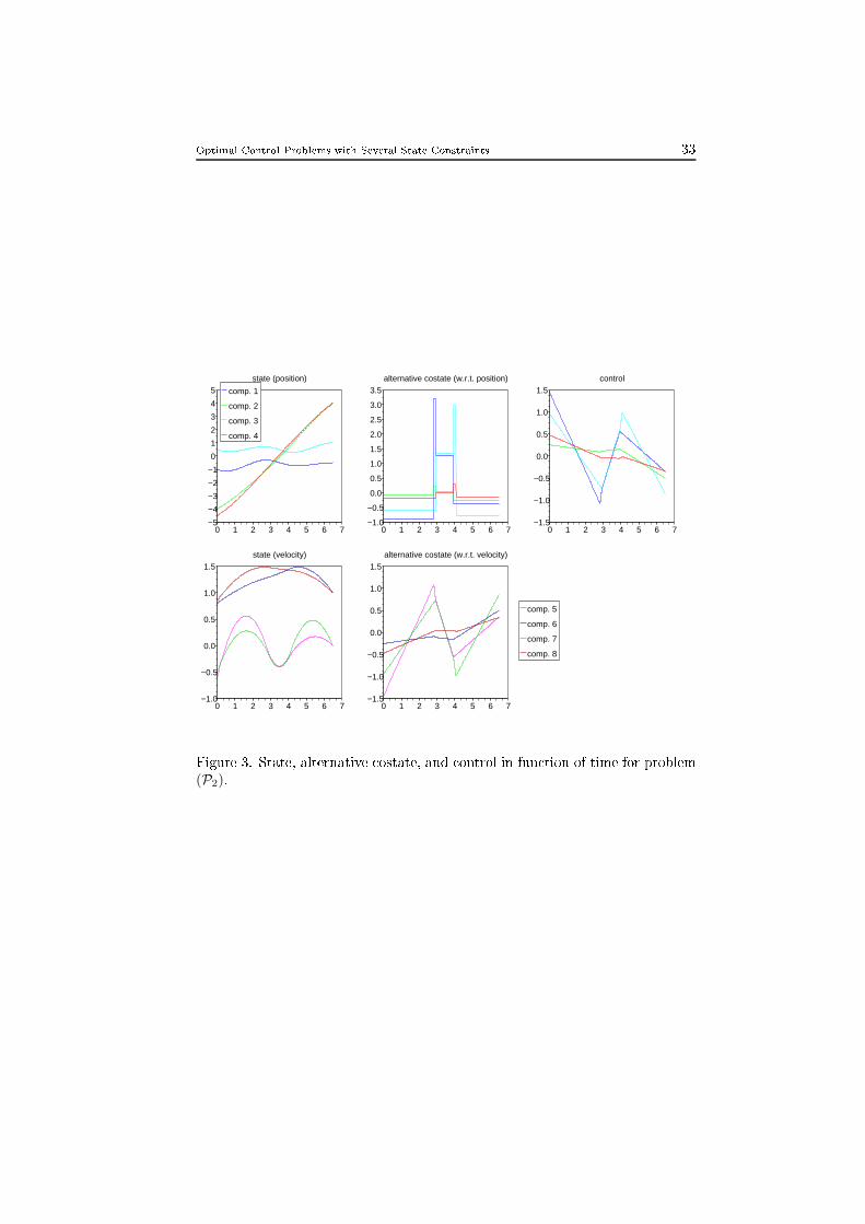
, σT ). (156)With Lemma 7, this implies that DF(θ)ω = δ i� π0 = πδ0 and the remaining omponents of ω are determined by (150)-(154), as to be proved.Remark 3 In view of the analysis of jun tion onditions in Bonnans and Her-mant (2009b) and Maurer (1979), onditions (142)-(143) are typi ally not sat-is�ed for boundary ar s of order greater than two. In that ase the shootingalgorithm is ill-posed sin e the variations of orresponding times annot be re- overed as in (151)-(152). In fa t, it is generally believed that boundary ar sof order greater than two are ill-posed. See on this subje t Robbins (1980) andMilyutin (2000).6. Numeri al appli ation: ollision avoidan eWe present here a numeri al appli ation of the shooting algorithm on two a a-demi problems involving three state onstraints. The latter modelize the prob-lem of obsta le avoidan e for two vehi les, assimilated to material points, witha onstraint of keeping a minimum distan e between them. The goal is to gofrom given initial positions to �nal ones by minimizing a ompromise between

Optimal Control Problems with Several State Constraints 27the �nal time and the energy spent by the ontrol. It is onvenient in the ex-amples to denote as e.g. y(t) the dependen e w.r.t. t. The problems under onsideration are, for the �rst order dynami s(P1)

min

∫ tf

0

(

1 + µ

4∑

i=1

u2i

)

dt

yi = ui, i = 1, . . . , 4, y(0) = y0, y(tf ) = yf , g(y) ≤ 0,and for the se ond order dynami s(P2)

min

∫ tf

0

(

1 + µ4∑

i=1

u2i

)

dt

yi = yi+4, yi+4 = ui, i = 1, . . . , 4, y(0) = y0, y(tf ) = yf ,

g(y) ≤ 0,with µ > 0. The Cartesian oordinates of the two vehi les in the plane aregiven respe tively by (y1, y2) and (y3, y4). The state onstraint g has three omponents: obsta les avoidan e (the obsta les are modelled by two parabola)g1(y) := −y1−b(y2−c)2−a ≤ 0, g2(y) := y3−b(y4+c)2−a ≤ 0, (157)where a, b > 0 and c are given parameters, and a minimum distan e onstraintbetween the two vehi les:

g3(y) := ρ2min − ((y1 − y3)

2 + (y2 − y4)2) ≤ 0, (158)with ρmin > 0. The �nal time tf is free. Note that by the well-known hange oftime s := t/tf , we re over the ase of a �xed �nal time. Due to the onstraint onthe �nal state, the �nal ondition in the shooting algorithm p(tf )−φ′(y(tf )) = 0is repla ed by the ondition y(tf ) − yf = 0.Remark 4 For the problems under onsideration, the stru ture of the traje -tory and initial values for the unknowns variables were guessed, making, ifne essary, several tries. Methods that automati ally determine the stru tureare presented in Bonnans and Hermant (2009b) Hermant (2009b) (when thereis however only one onstraint and one ontrol).6.1. First order state onstraintsWe solve problem (P1) using the shooting algorithm for the parameters

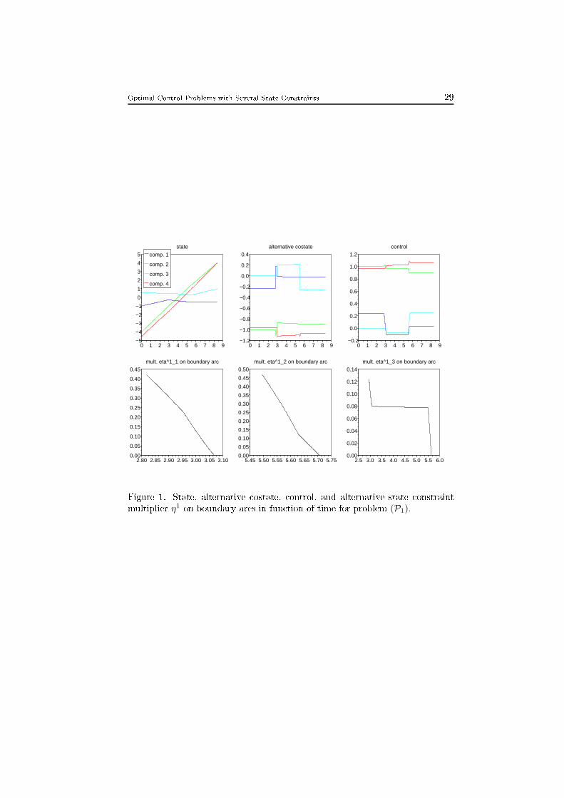
µ = 0.5, a = 0.3, b = 0.7, c = −1, ρmin = 1, (159)and initial and �nal onditions given byy0 = (−1, −4, 0.5, −4.5)⊤, yf = (−0.5, 4, 1, 4)⊤.

28 J.F. Bonnans and A. HermantEa h omponent of the state onstraint is a tive on a single boundary ar . Thestru ture of the traje tory, omposed by seven ar s, is given more pre isely inTable 1, where the jun tion times are given at beginning of ar s, and jumpparameters are at entry times.Ar 1 2 3 4 5 6 7A tive(s) onstraint(s) no 1 1, 3 3 2, 3 2 noJun tion time 0 2.82 2.95 3.07 5.49 5.62 5.71Jump parameter - 0.42 0.12 - 0.47 - -Table 1. Stru ture of problem (P1).The solution is plotted on Fig. 1. The initial ostate and �nal time arep0 =

−0.2412−1.00410.0040−0.9662

,

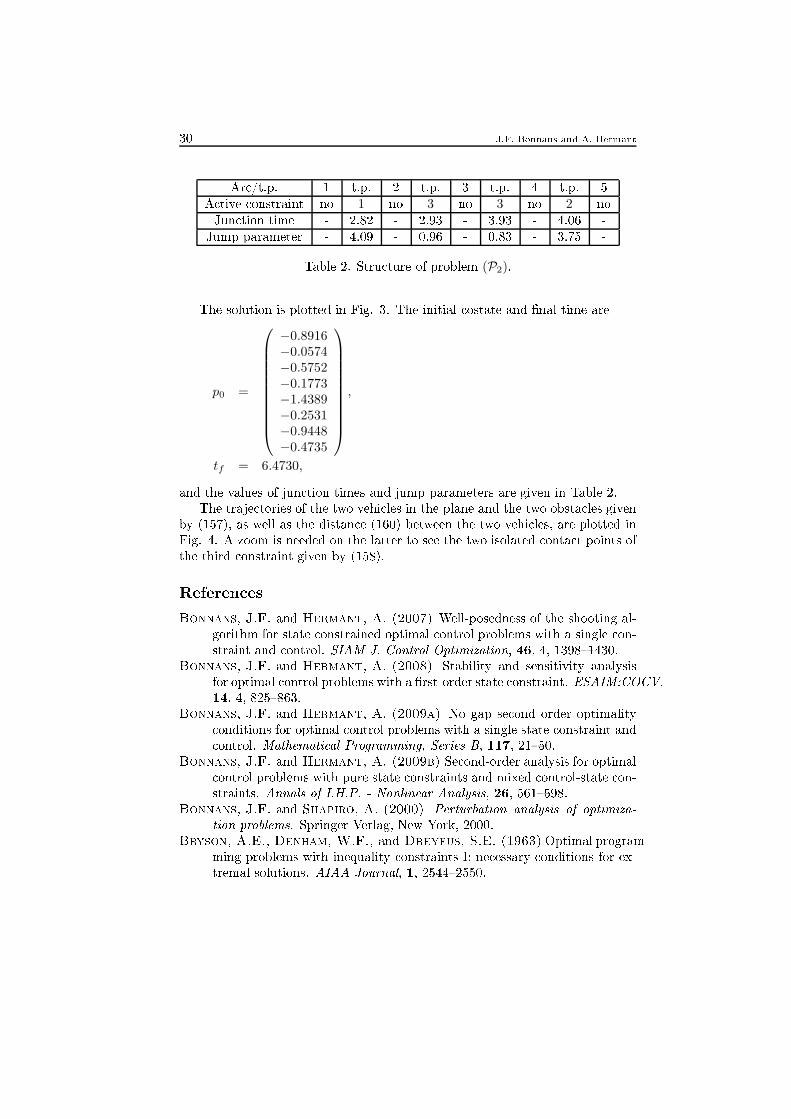
tf = 8.3605,and the jun tion times and jump parameters are given in Table 1.The three omponents of the alternative state onstraint multiplier η1i , i = 1to 3, are plotted along their respe tive boundary ar . We he k that the latterare de reasing, and hen e the ondition η = −η1 ≥ 0 of the minimum prin iple issatis�ed. The traje tories of the two vehi les in the plane and the two obsta lesgiven by (157), as well as the distan e

d :=√

(y1 − y3)2 + (y2 − y4)2 (160)between the two vehi les, are plotted on Fig. 2.6.2. Se ond order state onstraintsWe solve problem (P2) using the shooting algorithm for parameters given by(159) and initial and �nal onditions as follows:y0 = (−1, −4, 0.5, −4.5, −0.6, 0.8, −0.5, 0.85)⊤,

yf = (−0.5, 4, 1, 4, 0, 1, 0, 1)⊤.Ea h of the two �rst state onstraints are a tive at a single tou h point, while thethird is a tive at two tou h points. The stru ture of the traje tory, omposedby �ve ar s separated by four tou h points (t.p.), is given more pre isely inTable 2. We he k that the jumps parameters of the ostate at tou h points arenonnegative.

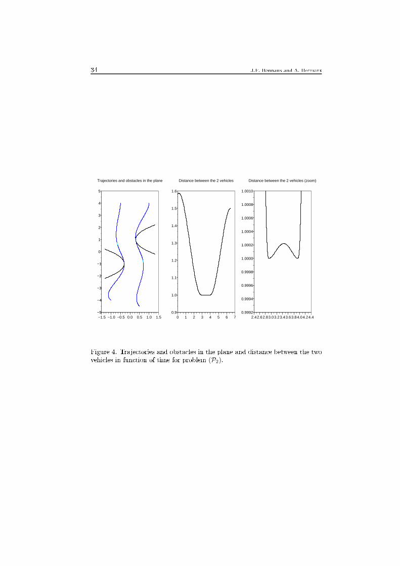
Optimal Control Problems with Several State Constraints 29

0 1 2 3 4 5 6 7 8 9−5

−4

−3

−2

−1

0

1

2

3

4

5state

0 1 2 3 4 5 6 7 8 9−1.2

−1.0

−0.8

−0.6

−0.4

−0.2

0.0

0.2

0.4alternative costate

0 1 2 3 4 5 6 7 8 9−0.2

0.0

0.2

0.4

0.6

0.8

1.0

1.2control

2.5 3.0 3.5 4.0 4.5 5.0 5.5 6.00.00

0.02

0.04

0.06

0.08

0.10

0.12

0.14mult. eta^1_3 on boundary arc

2.80 2.85 2.90 2.95 3.00 3.05 3.100.00

0.05

0.10

0.15

0.20

0.25

0.30

0.35

0.40

0.45mult. eta^1_1 on boundary arc

5.45 5.50 5.55 5.60 5.65 5.70 5.750.00

0.05

0.10

0.15

0.20

0.25

0.30

0.35

0.40

0.45

0.50mult. eta^1_2 on boundary arc

comp. 1

comp. 2

comp. 3

comp. 4

Figure 1. State, alternative ostate, ontrol, and alternative state onstraintmultiplier η1 on boundary ar s in fun tion of time for problem (P1).

30 J.F. Bonnans and A. HermantAr /t.p. 1 t.p. 2 t.p. 3 t.p. 4 t.p. 5A tive onstraint no 1 no 3 no 3 no 2 noJun tion time - 2.82 - 2.93 - 3.93 - 4.06 -Jump parameter - 4.09 - 0.96 - 0.83 - 3.75 -Table 2. Stru ture of problem (P2).The solution is plotted in Fig. 3. The initial ostate and �nal time arep0 =

−0.8916−0.0574−0.5752−0.1773−1.4389−0.2531−0.9448−0.4735

,

tf = 6.4730,and the values of jun tion times and jump parameters are given in Table 2.The traje tories of the two vehi les in the plane and the two obsta les givenby (157), as well as the distan e (160) between the two vehi les, are plotted inFig. 4. A zoom is needed on the latter to see the two isolated onta t points ofthe third onstraint given by (158).Referen esBonnans, J.F. and Hermant, A. (2007) Well-posedness of the shooting al-gorithm for state onstrained optimal ontrol problems with a single on-straint and ontrol. SIAM J. Control Optimization, 46, 4, 1398�1430.Bonnans, J.F. and Hermant, A. (2008) Stability and sensitivity analysisfor optimal ontrol problems with a �rst-order state onstraint. ESAIM:COCV,14, 4, 825�863.Bonnans, J.F. and Hermant, A. (2009a) No gap se ond order optimality onditions for optimal ontrol problems with a single state onstraint and ontrol. Mathemati al Programming, Series B, 117, 21�50.Bonnans, J.F. and Hermant, A. (2009b) Se ond-order analysis for optimal ontrol problems with pure state onstraints and mixed ontrol-state on-straints. Annals of I.H.P. - Nonlinear Analysis, 26, 561�598.Bonnans, J.F. and Shapiro, A. (2000) Perturbation analysis of optimiza-tion problems. Springer-Verlag, New York, 2000.Bryson, A.E., Denham, W.F., and Dreyfus, S.E. (1963)Optimal program-ming problems with inequality onstraints I: ne essary onditions for ex-tremal solutions. AIAA Journal, 1, 2544�2550.

Optimal Control Problems with Several State Constraints 31Hartl, R.F., Sethi, S.P., and Vi kson, R.G. (1995) A survey of the maxi-mum prin iples for optimal ontrol problems with state onstraints. SIAMReview, 37, 181�218.Hermant, A. (2008) Optimal ontrol of the atmospheri reentry of a spa eshuttle by an homotopy method. Rapport de Re her he RR 6627, INRIA,2008.Hermant, A. (2009a) Stability analysis of optimal ontrol problems with ase ond order state onstraint. SIAM J. Optimization, 20, 1, 104�129.Hermant, A. (2009b) Homotopy algorithm for optimal ontrol problems witha se ond-order state onstraint. Applied Mathemati s and Optimization,DOI:10.1007/s00245-009-9076-y.Ioffe, A.D., and Tihomirov, V.M. (1979) Theory of Extremal Problems.North-Holland Publishing Company, Amsterdam. Russian Edition: Nau-ka, Mos ow, 1974.Ja obson, D.H., Lele, M.M., and Speyer, J.L. (1971) New ne essary on-ditions of optimality for ontrol problems with state-variable inequality ontraints. J. of Mathemati al Analysis and Appli ations, 35, 255�284.Malanowski, K. (2007) Stability analysis for nonlinear optimal ontrol prob-lems subje t to state onstraints. SIAM J. Optim., 18, 3, 926�945 (ele -troni ).Malanowski, K. and Maurer, H. (1998) Sensitivity analysis for state on-strained optimal ontrol problems. Dis rete and Continuous Dynami alSystems, 4, 241�272.Malanowski, K. and Maurer, H. (2001) Sensitivity analysis for optimal ontrol problems subje t to higher order state onstraints. Ann. Oper.Res., 101, 43�73. Optimization with data perturbations, II.Maurer, H. (1979) On the minimum prin iple for optimal ontrol problemswith state onstraints. S hriftenreihe des Re henzentrum 41, UniversitätMünster.Milyutin, A. A. (2000) On a ertain family of optimal ontrol problems withphase onstraint. J. Math. S i. (New York), 100, 5, 2564�2571. Pon-tryagin Conferen e, 1, Optimal Control (Mos ow, 1998).Opfer, G., and Oberle, H.J. (1988) The derivation of ubi splines withobsta les by methods of optimization and optimal ontrol. Numeris heMathematik, 52, 17�31.Robbins, H.M. (1980) Jun tion phenomena for optimal ontrol with state-variable inequality onstraints of third order. J. of Optimization Theoryand Appli ations, 31, 85�99.

32 J.F. Bonnans and A. Hermant

−1.5 −1.0 −0.5 0.0 0.5 1.0 1.5−5

−4

−3

−2

−1

0

1

2

3

4

5

Trajectories and obstacles in the plane

0 1 2 3 4 5 6 7 8 91.0

1.1

1.2

1.3

1.4

1.5

1.6

Distance between the 2 vehicles

Figure 2. Traje tories and obsta les in the plane and distan e between the twovehi les in fun tion of time for problem (P1)..

Optimal Control Problems with Several State Constraints 33

0 1 2 3 4 5 6 7−5

−4

−3

−2

−1

0

1

2

3

4

5state (position)

0 1 2 3 4 5 6 7−1.0

−0.5

0.0

0.5

1.0

1.5state (velocity)

0 1 2 3 4 5 6 7−1.0

−0.5

0.0

0.5

1.0

1.5

2.0

2.5

3.0

3.5alternative costate (w.r.t. position)

0 1 2 3 4 5 6 7−1.5

−1.0

−0.5

0.0

0.5

1.0

1.5alternative costate (w.r.t. velocity)

0 1 2 3 4 5 6 7−1.5

−1.0

−0.5

0.0

0.5

1.0

1.5control

comp. 1

comp. 2

comp. 3

comp. 4

comp. 5

comp. 6

comp. 7

comp. 8

Figure 3. State, alternative ostate, and ontrol in fun tion of time for problem(P2).

34 J.F. Bonnans and A. Hermant

−1.5 −1.0 −0.5 0.0 0.5 1.0 1.5−5

−4

−3

−2

−1

0

1

2

3

4

5

Trajectories and obstacles in the plane

0 1 2 3 4 5 6 70.9

1.0

1.1

1.2

1.3

1.4

1.5

1.6

Distance between the 2 vehicles

2.42.62.83.03.23.43.63.84.04.24.40.9992

0.9994

0.9996

0.9998

1.0000

1.0002

1.0004

1.0006

1.0008

1.0010

Distance between the 2 vehicles (zoom)

Figure 4. Traje tories and obsta les in the plane and distan e between the twovehi les in fun tion of time for problem (P2).