Embed Size (px)
Citation preview
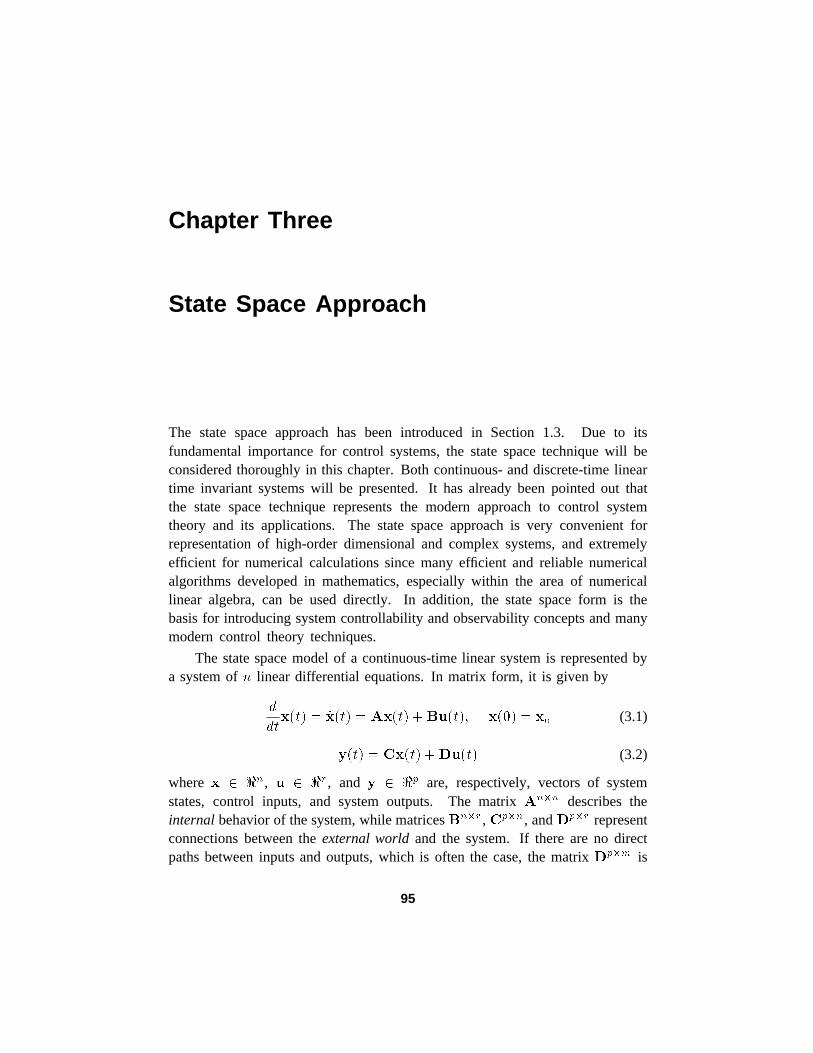
Chapter Three
State Space Approach
The state space approach has been introduced in Section 1.3. Due to itsfundamental importance for control systems, the state space technique will beconsidered thoroughly in this chapter. Both continuous- and discrete-time lineartime invariant systems will be presented. It has already been pointed out thatthe state space technique represents the modern approach to control systemtheory and its applications. The state space approach is very convenient forrepresentation of high-order dimensional and complex systems, and extremelyefficient for numerical calculations since many efficient and reliable numericalalgorithms developed in mathematics, especially within the area of numericallinear algebra, can be used directly. In addition, the state space form is thebasis for introducing system controllability and observability concepts and manymodern control theory techniques.
The state space model of a continuous-time linear system is represented bya system ofn linear differential equations. In matrix form, it is given by
d
dtx(t) = _x(t) = Ax(t) +Bu(t); x(0) = x0 (3.1)
y(t) = Cx(t) +Du(t) (3.2)
where x 2 <n, u 2 <r, and y 2 <p are, respectively, vectors of systemstates, control inputs, and system outputs. The matrixAn�n describes theinternal behavior of the system, while matricesBn�r ,Cp�n, andDp�r representconnections between theexternal worldand the system. If there are no directpaths between inputs and outputs, which is often the case, the matrixDp�m is
95
96 STATE SPACE APPROACH
zero. It is assumed in this book that all matrices in (3.1) and (3.2) are timeinvariant. Studying linear control systems with time varying coefficient matricesrequires knowledge of some advanced topics in mathematics (see for exampleChen, 1984; see also Section 10.1).
The state space model for linear discrete-time control systems has exactly thesame form as (3.1) and (3.2) with differential equations replaced by differenceequations, that is
x(k +1) =Adx(k) +Bdu(k); x(0) = x0 (3.3)
y(k) = Cdx(k) +Ddu(k) (3.4)
All vectors and matrices defined in (3.3) and (3.4) have the same dimensions ascorresponding ones given in (3.1) and (3.2). In this chapter, we present and derivein detail the main state space concepts for continuous-time linear control systemsand then give the corresponding interpretations in the discrete-time domain.
The chapter is organized as follows. In Section 3.1 several systematicmethods for obtaining the state space form from differential equations and transferfunctions are developed. The time response of linear systems given in the stateform is considered in Section 3.2. The corresponding results for discrete-timesystems, and the procedure for discretization of continuous-time systems leadingto discrete-time models, are given in Section 3.3. The concepts of the systemcharacteristic equation, eigenvalues, and eigenvectors and their use in controlsystem theory are presented in Section 3.4. At the end of the chapter, in Section3.5, three MATLAB laboratory experiments are outlined.
Chapter Objectives
The dynamical systems considered in this book are either described bydifferential/difference equations or given in the form of system transfer functions.One of the goals is to present procedures for obtaining the state space forms eitherfrom differential/difference equations or from transfer functions. In that respectstudents will be exposed to four standard state space forms, known as canonicalforms: the phase variable form or controller form, the observer form, the modalform, and the Jordan form.
Another important objective is to show students how to analyze linearsystems given in the state space form, i.e. how to find responses (state variablesand outputs) of the corresponding state space models to any input signal (control
STATE SPACE APPROACH 97
input). A working knowledge of undergraduate linear algebra and the basictheory of differential equations is helpful for complete understanding of thischapter. Some useful results on linear algebra are given in Appendix C. Studentswithout a strong background in these topics may consult any undergraduate text,(for example, Fraleigh and Beauregard, 1990; Boyce and DiPrima, 1992).
3.1 State Space ModelsIn this section we study state space models of continuous-time linear systems.The corresponding results for discrete-time systems, obtained via duality with thecontinuous-time models, are given in Section 3.3.
The state space model of a continuous-time dynamic system can be derivedeither from the system model given in the time domain by a differential equationor from its transfer function representation. Both cases will be considered in thissection. Four state space forms—the phase variable form (controller form), theobserver form, the modal form, and the Jordan form—which are often used inmodern control theory and practice, are presented.
3.1.1 The State Space Model and Differential EquationsConsider a generalnth-order model of a dynamic system represented by annth-order differential equation
dny(t)
dtn+ an�1
dn�1y(t)dtn�1
+ � � �+ a1dy(t)
dt+ a0y(t)
= bndnu(t)
dtn+ bn�1
dn�1u(t)dtn�1
+ � � �+ b1du(t)
dt+ b0u(t)
(3.5)
At this point we assume that all initial conditions for the above differentialequation, i.e. y(0�); dy(0�)=dt; :::; dn�1y(0�)=dtn�1, are equal to zero. Wewill show later how to take into account the effect of initial conditions.
In order to derive a systematic procedure that transforms a differentialequation of ordern to a state space form representing a system ofn first-orderdifferential equations, we first start with a simplified version of (3.5), namely westudy the case when no derivatives with respect to the input are present
dny(t)
dtn+ an�1
dn�1y(t)dtn�1
+ � � �+ a1dy(t)
dt+ a0y(t) = u(t) (3.6)
98 STATE SPACE APPROACH
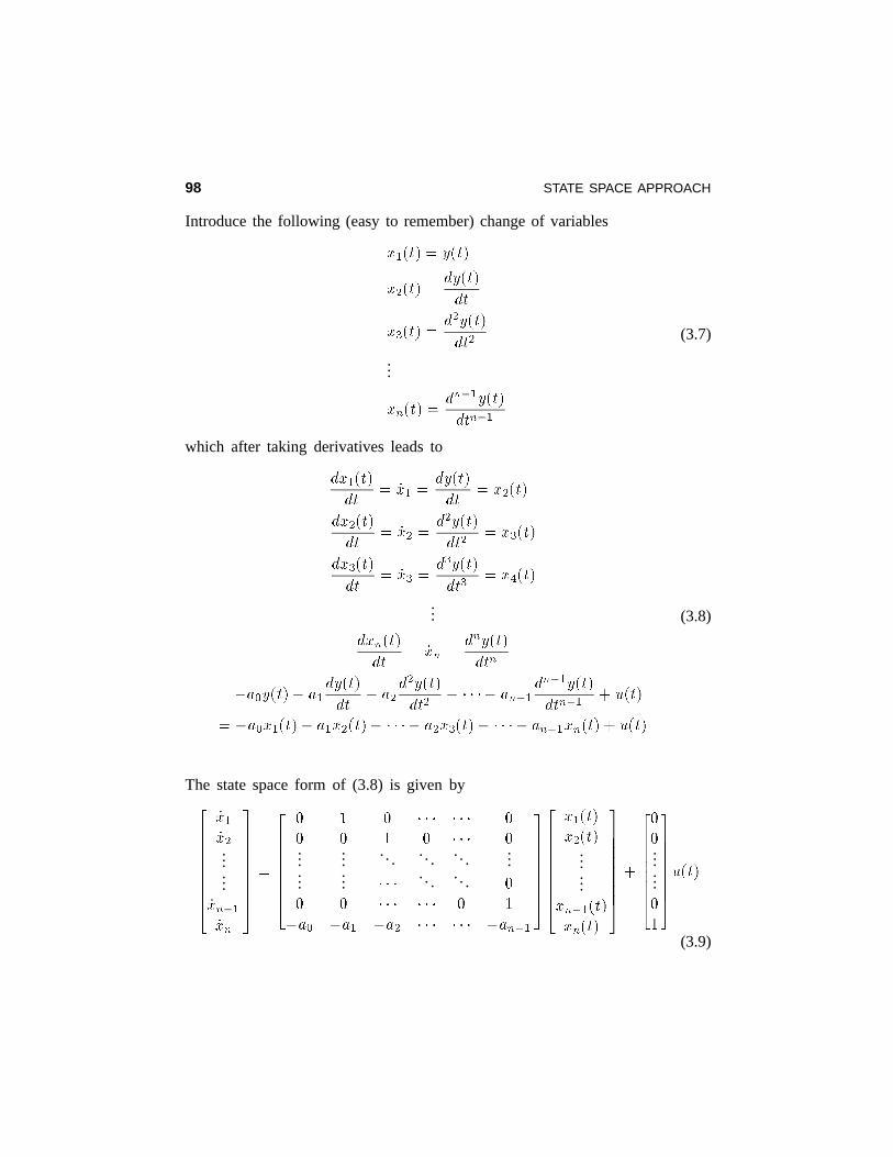
Introduce the following (easy to remember) change of variables
x1(t) = y(t)
x2(t) =dy(t)
dt
x3(t) =d2y(t)
dt2
...
xn(t) =dn�1y(t)dtn�1
(3.7)
which after taking derivatives leads to
dx1(t)
dt= _x1 =
dy(t)
dt= x2(t)
dx2(t)
dt= _x2 =
d2y(t)
dt2= x3(t)
dx3(t)
dt= _x3 =
d3y(t)
dt3= x4(t)
...
dxn(t)
dt= _xn =
dny(t)
dtn
= �a0y(t)� a1dy(t)
dt� a2
d2y(t)
dt2� � � � � an�1
dn�1y(t)dtn�1
+ u(t)
= �a0x1(t)� a1x2(t)� � � � � a2x3(t)� � � � � an�1xn(t) + u(t)
(3.8)
The state space form of (3.8) is given by266666664
_x1_x2......
_xn�1_xn
377777775=
26666664
0 1 0 � � � � � � 0
0 0 1 0 � � � 0...
..... . .. . .. .
......
... � � � .. . .. . 0
0 0 � � � � � � 0 1
�a0 �a1 �a2 � � � � � � �an�1
37777775
266666664
x1(t)
x2(t)......
xn�1(t)xn(t)
377777775+
26666664
0
0......0
1
37777775u(t)(3.9)
STATE SPACE APPROACH 99
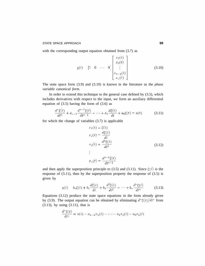
with the corresponding output equation obtained from (3.7) as
y(t) = [1 0 � � � 0 ]
2666664x1(t)
x2(t)...
xn�1(t)xn(t)
3777775 (3.10)
The state space form (3.9) and (3.10) is known in the literature as thephasevariable canonical form.
In order to extend this technique to the general case defined by (3.5), whichincludes derivatives with respect to the input, we form an auxiliary differentialequationof (3.5) having the form of (3.6) as
dn�(t)
dtn+ an�1
dn�1�(t)dtn�1
+ � � �+ a1d�(t)
dt+ a0�(t) = u(t) (3.11)
for which the change of variables (3.7) is applicable
x1(t) = �(t)
x2(t) =d�(t)
dt
x3(t) =d2�(t)
dt2
...
xn(t) =dn�1�(t)dtn�1
(3.12)
and then apply the superposition principle to (3.5) and (3.11). Since�(t) is theresponse of (3.11), then by the superposition property the response of (3.5) isgiven by
y(t) = b0�(t) + b1d�(t)
dt+ b2
d2�(t)
dt2+ � � �+ bn
dn�(t)
dtn(3.13)
Equations (3.12) produce the state space equations in the form already givenby (3.9). The output equation can be obtained by eliminatingdn�(t)=dtn from(3.13), by using (3.11), that is
dn�(t)
dtn= u(t)� an�1xn(t)� � � � � a1x2(t)� a0x1(t)
100 STATE SPACE APPROACH
This leads to the output equation
y(t) = [(b0 � a0bn) (b1 � a1bn) � � � (bn�1 � an�1bn) ]
2664x1(t)
x2(t)...
xn(t)
3775 + bnu(t)
(3.14)It is interesting to point out that forbn = 0, which is almost always the case, theoutput equation also has an easy-to-remember form given by
y(t) = [b0 b1 � � � bn�1 ]
2664x1(t)
x2(t)...
xn(t)
3775 (3.15)
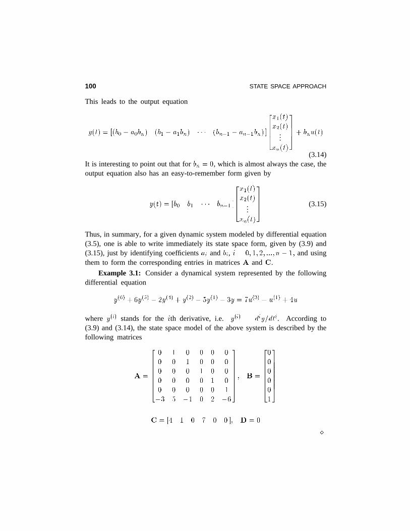
Thus, in summary, for a given dynamic system modeled by differential equation(3.5), one is able to write immediately its state space form, given by (3.9) and(3.15), just by identifying coefficientsai andbi, i = 0; 1;2; :::;n � 1; and usingthem to form the corresponding entries in matricesA andC.
Example 3.1: Consider a dynamical system represented by the followingdifferential equation
y(6) +6y(5) � 2y(4) + y(2) � 5y(1) + 3y = 7u(3) + u(1) + 4u
where y(i) stands for theith derivative, i.e. y(i) = diy=dti. According to(3.9) and (3.14), the state space model of the above system is described by thefollowing matrices
A =
26666664
0 1 0 0 0 0
0 0 1 0 0 0
0 0 0 1 0 0
0 0 0 0 1 0
0 0 0 0 0 1
�3 5 �1 0 2 �6
37777775; B =
26666664
0
0
0
0
0
1
37777775C = [4 1 0 7 0 0 ]; D = 0
�
STATE SPACE APPROACH 101
3.1.2 State Space Variables from Transfer Functions
In this section, we present two methods, known as direct and parallel program-ming techniques, which can be used for obtaining state space models from systemtransfer functions. For simplicity, like in the previous subsection, we consideronly single-input single-output systems.
The resulting state space models may or may not contain all the modesof the original transfer function, where by transfer function modes we meanpoles of the original transfer function (before zero-pole cancellation, if any, takesplace). If some zeros and poles in the transfer function are cancelled, then theresulting state space model will be of reduced order and the corresponding modeswill not appear in the state space model. This problem of system reducibilitywill be addressed in detail in Chapter 5 after we have introduced the systemcontrollability and observability concepts.
In the following, we first use direct programming techniques to derive thestate space forms known as the controller canonical form and the observercanonical form; then, by the method of parallel programing, the state spaceforms known as modal canonical form and Jordan canonical form are obtained.
The Direct Programming Technique and Controller Canonical Form
This technique is convenient in the case when the plant transfer function isgiven in a nonfactorized polynomial form
Y (s)
U(s)=
bnsn + bn�1sn�1 + � � �+ b1s+ b0
sn + an�1sn�1 + � � �+ a1s+ a0(3.16)
For this system an auxiliary variableV (s) is introduced such that the transferfunction is split as
V (s)
U(s)=
1
sn + an�1sn�1 + � � �+ a1s+ a0(3.17a)
Y (s)
V (s)= bns
n + bn�1sn�1 + � � �+ b1s+ b0 (3.17b)
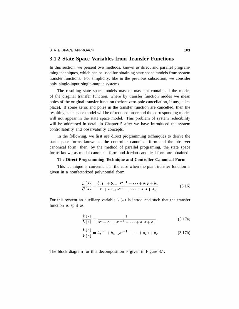
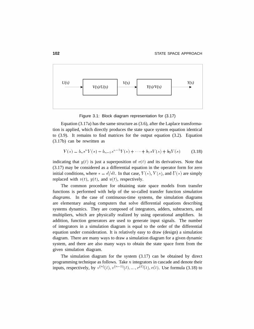
The block diagram for this decomposition is given in Figure 3.1.
102 STATE SPACE APPROACH
U(s) V(s)V(s)/U(s) Y(s)/V(s)
Y(s)
Figure 3.1: Block diagram representation for (3.17)
Equation (3.17a) has the same structure as (3.6), after the Laplace transforma-tion is applied, which directly produces the state space system equation identicalto (3.9). It remains to find matrices for the output equation (3.2). Equation(3.17b) can be rewritten as
Y (s) = bnsnV (s) + bn�1s
n�1V (s) + � � �+ b1sV (s) + b0V (s) (3.18)
indicating thaty(t) is just a superposition ofv(t) and its derivatives. Note that(3.17) may be considered as a differential equation in the operator form for zeroinitial conditions, wheres � d=dt. In that case,V (s), Y (s), andU(s) are simplyreplaced withv(t), y(t), andu(t), respectively.
The common procedure for obtaining state space models from transferfunctions is performed with help of the so-called transfer functionsimulationdiagrams. In the case of continuous-time systems, the simulation diagramsare elementary analog computers that solve differential equations describingsystems dynamics. They are composed of integrators, adders, subtracters, andmultipliers, which are physically realized by using operational amplifiers. Inaddition, function generators are used to generate input signals. The numberof integrators in a simulation diagram is equal to the order of the differentialequation under consideration. It is relatively easy to draw (design) a simulationdiagram. There are many ways to draw a simulation diagram for a given dynamicsystem,and there are also many ways to obtain the state space form from thegiven simulation diagram.
The simulation diagram for the system (3.17) can be obtained by directprogramming technique as follows. Taken integrators in cascade and denote theirinputs,respectively, byv(n)(t); v(n�1)(t); :::; v(1)(t); v(t). Use formula (3.18) to
STATE SPACE APPROACH 103
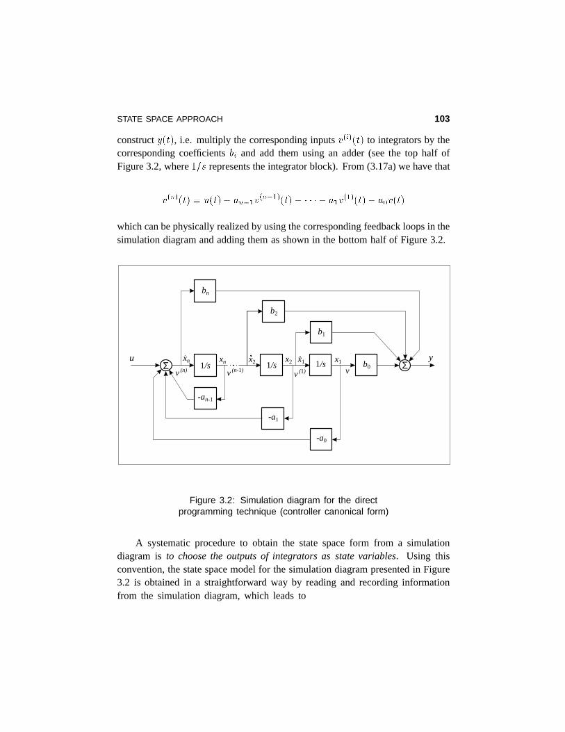
constructy(t), i.e. multiply the corresponding inputsv(i)(t) to integrators by thecorresponding coefficientsbi and add them using an adder (see the top half ofFigure 3.2, where1=s represents the integrator block). From (3.17a) we have that
v(n)(t) = u(t)� an�1v(n�1)(t)� � � � � a1v
(1)(t)� a0v(t)
which can be physically realized by using the corresponding feedback loops in thesimulation diagram and adding them as shown in the bottom half of Figure 3.2.
x1x1x2x2xnxn
v (n)1/s1/s ΣΣ
u yb0
bn
b2
b1
-a0
-a1
-an-1
v (n-1)v (1) v
1/s
Figure 3.2: Simulation diagram for the directprogramming technique (controller canonical form)
A systematic procedure to obtain the state space form from a simulationdiagram isto choose the outputs of integrators as state variables. Using thisconvention, the state space model for the simulation diagram presented in Figure3.2 is obtained in a straightforward way by reading and recording informationfrom the simulation diagram, which leads to
104 STATE SPACE APPROACH
_x(t) =
26666664
0 1 0 � � � � � � 0
0 0 1 0 � � � 0...
..... . .. . .. .
......
......
.. . .. . 0
0 0 0 � � � 0 1
�a0 �a1 �a2 � � � � � � �an�1
37777775x(t) +26666664
0
0......0
1
37777775u(t) (3.19)
and
y(t) = [(b0 � a0bn) (b1 � a1bn) � � � (bn�1 � an�1bn) ]x(t) + bnu(t)
(3.20)
This form of the system model is called thecontroller canonical form. Itis identical to the one obtained in the previous section—equations (3.9) and(3.14). Controller canonical form plays an important role in control theory sinceit represents the so-called controllable system. System controllability is one of themain concepts of modern control theory. It will be studied in detail in Chapter 5.
It is important to point out that there are many state space forms for a givendynamical system, and that all of them are related by linear transformations.More about this fact, together with the development of other important state spacecanonical forms, can be found in Kailath (1980; see also similarity transformationin Section 3.4).
Note that the MATLAB functiontf2ss produces the state space form fora given transfer function, in fact, it produces the controller canonical form.
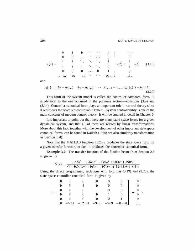
Example 3.2: The transfer function of the flexible beam from Section 2.6is given by
G(s) =1:65s4 � 0:331s3 � 576s2 + 90:6s+19080
s6 +0:996s5 +463s4 + 97:8s3 + 12131s2 + 8:11s
Using the direct programming technique with formulas (3.19) and (3.20), thestate space controller canonical form is given by
_x =
26666664
0 1 0 0 0 0
0 0 1 0 0 0
0 0 0 1 0 0
0 0 0 0 1 0
0 0 0 0 0 1
0 �8:11 �12131 �97:8 �463 �0:996
37777775x+26666664
0
0
0
0
0
1
37777775u
STATE SPACE APPROACH 105
andy = [19080 90:6 �576 �0:331 1:65 0 ]x
�Direct Programming Technique and Observer Canonical Form
In addition to controller canonical form,observercanonical formis relatedto another important concept of modern control theory: system observability.Observer canonical form has a very simple structure and represents an observablesystem. The concept of linear system observability will be considered thoroughlyin Chapter 5.
Observer canonical form can be derived as follows. Equation (3.16) is writtenin the form
Y (s)�sn + an�1sn�1 + � � �+ a1s+ a0
�= U(s)
�bns
n + bn�1sn�1 + � � �+ b1s+ b0� (3.21)
and expressed as
Y (s) = � 1
sn�an�1sn�1 + � � �+ a1s+ a0
�Y (s)
+1
snU(s)
�bns
n + bn�1sn�1 + � � �+ b1s+ b0� (3.22)
leading to
Y (s) = �1
san�1Y (s)� 1
s2an�2Y (s)� � � � � 1
sn�1a1Y (s)� 1
sna0Y (s)
+ bnU(s) +1
sbn�1U(s) +
1
s2bn�2U(s) + � � �+ 1
sn�1b1U(s) +
1
snb0U(s)
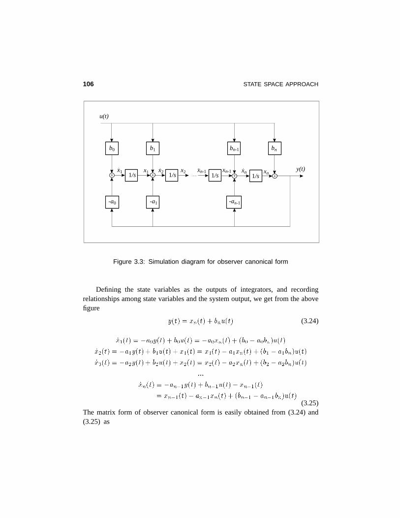
(3.23)This relationship can be implemented by using a simulation diagram composedof n integrators in a cascade, and letting the corresponding signals to passthrough the specified number of integrators. For example, terms containing1=s
should pass through only one integrator, signalsan�2y(t) and bn�2u(t) shouldpass through two integrators, and so on. Finally, signalsa0y(t) and b0u(t)
should be integratedn-times, i.e. they must pass through alln integrators. Thecorresponding simulation diagram is given in Figure 3.3.
106 STATE SPACE APPROACH
b0
u(t)
y(t)x2
-a0
+ 1/sx2
b1
-a1
+ 1/sxn-1 xn1/s
xn-1 xn
bn-1
-an-1
+ 1/s
bn
+x1x1
Figure 3.3: Simulation diagram for observer canonical form
Defining the state variables as the outputs of integrators, and recordingrelationships among state variables and the system output, we get from the abovefigure
y(t) = xn(t) + bnu(t) (3.24)
_x1(t) = �a0y(t) + b0u(t) = �a0xn(t) + (b0 � a0bn)u(t)
_x2(t) = �a1y(t) + b1u(t) + x1(t) = x1(t)� a1xn(t) + (b1 � a1bn)u(t)
_x3(t) = �a2y(t) + b2u(t) + x2(t) = x2(t)� a2xn(t) + (b2 � a2bn)u(t)
:::
_xn(t) = �an�1y(t) + bn�1u(t) + xn�1(t)= xn�1(t)� an�1xn(t) + (bn�1 � an�1bn)u(t)
(3.25)The matrix form of observer canonical form is easily obtained from (3.24) and(3.25) as
STATE SPACE APPROACH 107
_x(t) =
266666664
0 0 . . . . . . 0 �a01 0 . . . . . . 0 �a1
0 1.. . . . .
... �a2... 0 1
.. ....
......
..... . .. . 0 �an�2
0 0 . . . 0 1 �an�1
377777775x(t) +
266666664
b0 � a0bnb1 � a1bnb2 � a2bn
...
...bn�1 � an�1bn
377777775u(t) (3.26)
andy(t) = [0 � � � 0 1 ]x(t) + bnu(t) (3.27)
Example 3.3: The observer canonical form for the flexible beam fromExample 3.2 is given by
_x =
26666664
0 0 0 0 0 0
1 0 0 0 0 �8:11
0 1 0 0 0 �12131
0 0 1 0 0 �97:8
0 0 0 1 0 �463
0 0 0 0 1 �0:996
37777775x+26666664
19080
90:6
�576
�0:331
1:65
0
37777775u
andy = [0 0 0 0 0 1 ]x
�Observer canonical form is very useful for computer simulation of linear
dynamical systems since it allows the effect of the system initial conditions to betaken into account. Thus, this form represents an observable system, in the senseto be defined in Chapter 5, which means that all state variables have an impact onthe system output, and vice versa, that from the system output and state equationsone is able to reconstruct the state variables at any time instant, and of course atzero, and thus, determinex1(0); x2(0); :::; xn(0) in terms of the original initialconditionsy(0�); dy(0�)=dt; :::; dn�1y(0�)=dtn�1. For more details see Section5.5 for a subtopic on the observability role in analog computer simulation.
Parallel Programming Technique
For this technique we distinguish two cases: distinct real roots and multiplereal roots of the system transfer function denominator.
108 STATE SPACE APPROACH
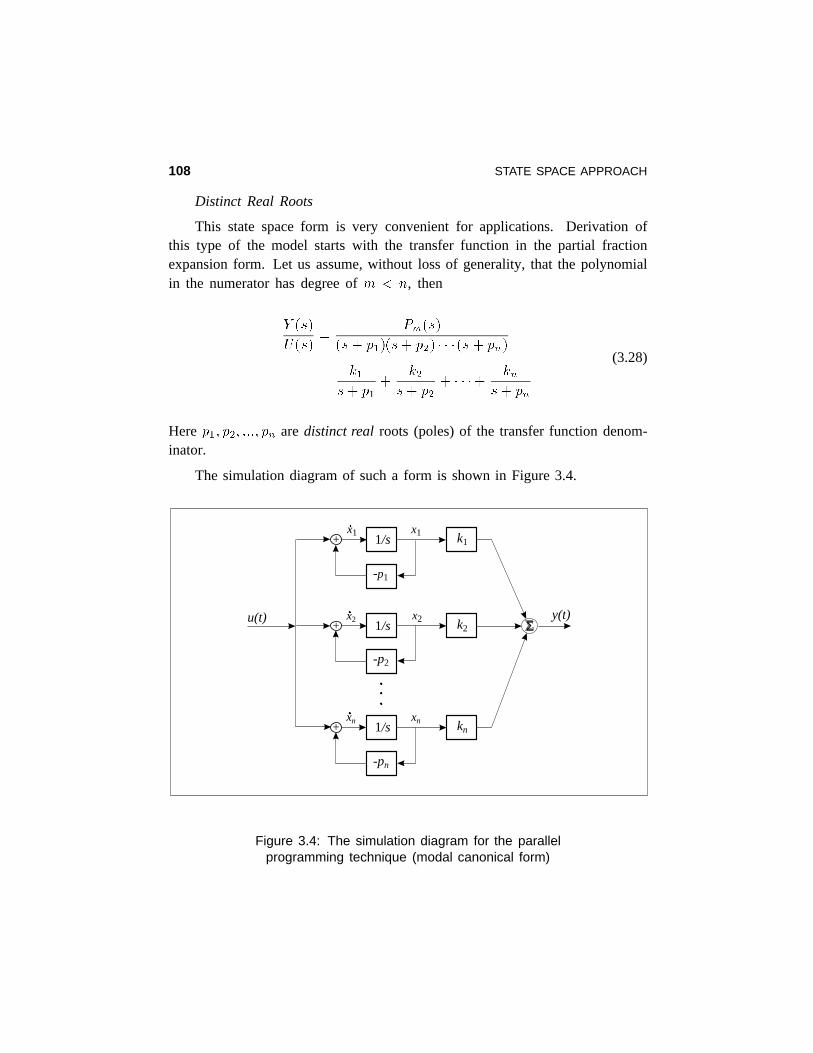
Distinct Real Roots
This state space form is very convenient for applications. Derivation ofthis type of the model starts with the transfer function in the partial fractionexpansion form. Let us assume, without loss of generality, that the polynomialin the numerator has degree ofm < n, then
Y (s)
U(s)=
Pm(s)
(s+ p1)(s+ p2) � � � (s+ pn)
=k1
s + p1+
k2s+ p2
+ � � �+ kns+ pn
(3.28)
Herep1; p2; :::; pn aredistinct real roots (poles) of the transfer function denom-inator.
The simulation diagram of such a form is shown in Figure 3.4.
u(t) y(t)Σ
x2x2
-p2
+ k21/s
x1x1
-p1
+ k11/s
xnxn
-pn
+ kn1/s
Figure 3.4: The simulation diagram for the parallelprogramming technique (modal canonical form)
STATE SPACE APPROACH 109
The state space model derived from this simulation diagram is given by
_x(t) =
2666664�p1 0 � � � � � � 0
0 �p2. .. � � � 0
..... . . .. . ..
......
.... .. . .. 0
0 0 � � � 0 �pn
3777775x(t) +2666641
1......1
377775u(t)
y(t) = [k1 k2 � � � � � � kn ]x(t)
(3.29)
This form is known in the literature as themodal canonical form(also knownas uncoupled form).
Example 3.4: Find the state space model of a system described by thetransfer function
Y (s)
U(s)=
(s+ 5)(s+4)
(s+ 1)(s+2)(s+ 3)
using both direct and parallel programming techniques.
The nonfactorized transfer function is
Y (s)
U(s)=
s2 + 9s+ 20
s3 + 6s2 + 11s+ 6
and the state space form obtained by using (3.19) and (3.20) of the directprogramming technique is
_x =
24 0 1 0
0 0 1
�6 �11 �6
35x+
24001
35uy = [20 9 1 ]x
Note that the MATLAB functiontf2ss produces
_x =
24�6 �11 �6
1 0 0
0 1 0
35x+
24100
35uy = [1 9 20 ]x
110 STATE SPACE APPROACH
which only indicates a permutation in the state space variables, that is
x =
240 0 1
0 1 0
1 0 0
35xEmploying the partial fraction expansion (which can be obtained by the
MATLAB function residue), the transfer function is written as
Y (s)
U(s)=
(s+5)(s+ 4)
(s+ 1)(s+ 2)(s+ 3)=
6
s +1� 6
s+ 2+
1
s+ 3
The state space model, directly written using (3.29), is
_x =
24�1 0 0
0 �2 0
0 0 �3
35x+
24111
35uy = [6 �6 1 ]x
�Note that the parallel programming technique presented is valid only for the
case of real distinct roots. If complex conjugate roots appear they should becombined in pairs corresponding to the second-order transfer functions, whichcan be independently implemented as demonstrated in the next example.
Example 3.5: Let a transfer function containing a pair of complex conjugateroots be given by
G(s) =4
s + 1� j+
4
s+ 1 + j+
2
s+ 5+
3
s + 10
We first group the complex conjugate poles in a second-order transfer function,that is
G(s) =8s+8
s2 + 2s+ 2+
2
s + 5+
3
s +10
Then, distinct real poles are implemented like in the case of parallel programming.A second-order transfer function, corresponding to the pair of complex conjugatepoles, is implemented using direct programming, and added in parallel to the first-order transfer functions corresponding to the real poles. The simulation diagram
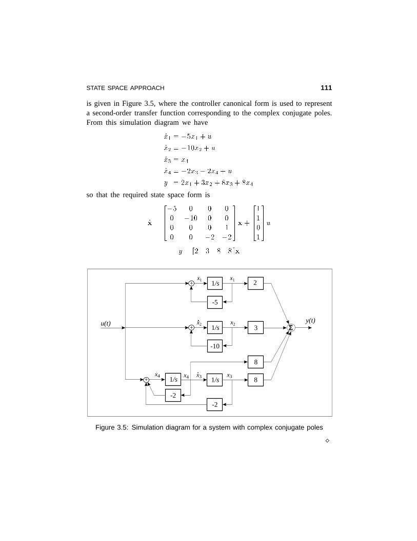
STATE SPACE APPROACH 111
is given in Figure 3.5, where the controller canonical form is used to representa second-order transfer function corresponding to the complex conjugate poles.From this simulation diagram we have
_x1 = �5x1 + u
_x2 = �10x2 + u
_x3 = x4
_x4 = �2x3 � 2x4 + u
y = 2x1 +3x2 + 8x3 + 8x4
so that the required state space form is
_x =
2664�5 0 0 0
0 �10 0 0
0 0 0 1
0 0 �2 �2
3775x+
26641
1
0
1
3775uy = [2 3 8 8 ]x
u(t) y(t)Σ
x2x2
-10
+ 31/s
x1x1
-5
+ 21/s
x4 x3 x3x4
-2-2
+ 8
8
1/s 1/s
Figure 3.5: Simulation diagram for a system with complex conjugate poles
�
112 STATE SPACE APPROACH
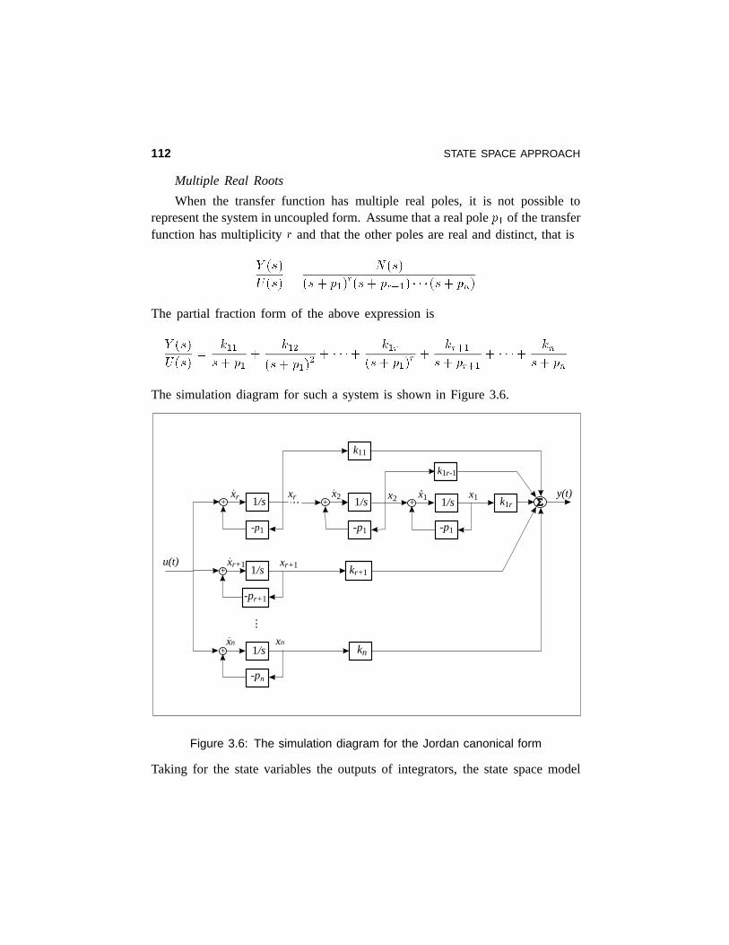
Multiple Real Roots
When the transfer function has multiple real poles, it is not possible torepresent the system in uncoupled form. Assume that a real polep1 of the transferfunction has multiplicityr and that the other poles are real and distinct, that is
Y (s)
U(s)=
N(s)
(s+ p1)r(s+ pr+1) � � � (s+ pn)
The partial fraction form of the above expression is
Y (s)
U(s)=
k11s+ p1
+k12
(s+ p1)2 + � � �+ k1r
(s+ p1)r +
kr+1s+ pr+1
+ � � �+ kns+ pn
The simulation diagram for such a system is shown in Figure 3.6.
y(t)Σ
k1r-1
k11
u(t)
x2
-p1
+ 1/sxrxr
-p1
+ 1/s
xr+ 1
-pr+ 1
+ kr+ 11/s
xn
-pn
+ 1/s kn
xr+ 1
xn
x2 x1x1
-p1
+ k1r1/s
Figure 3.6: The simulation diagram for the Jordan canonical form
Taking for the state variables the outputs of integrators, the state space model
STATE SPACE APPROACH 113
is obtained as follows
A =
266666666666666664
�p1 1 0 � � � � � � 0 0 � � � � � � 0
0 �p1 1 0 � � � 0 0 � � � � � � 0...
. .. .. . . .. . .....
......
......
0 � � � 0 �p1 1 0...
......
...0 � � � � � � 0 �p1 1 0 � � � � � � 0
0 � � � � � � � � � 0 �p1 0 � � � � � � 0
0 0 � � � � � � � � � 0 �pr+1 0 � � � 0
0 0 � � � � � � � � � 0. .. �pr+2
.. ....
......
......
......
.... .. .. . 0
0 0 � � � � � � � � � 0 0 � � � 0 �pn
377777777777777775(3.30)
B = [0 0 � � � � � � 0 1 1 � � � � � � 1 ]T
C = [k1r k1r�1 � � � � � � k12 k11 kr+1 kr+2 � � � kn ]; D = 0
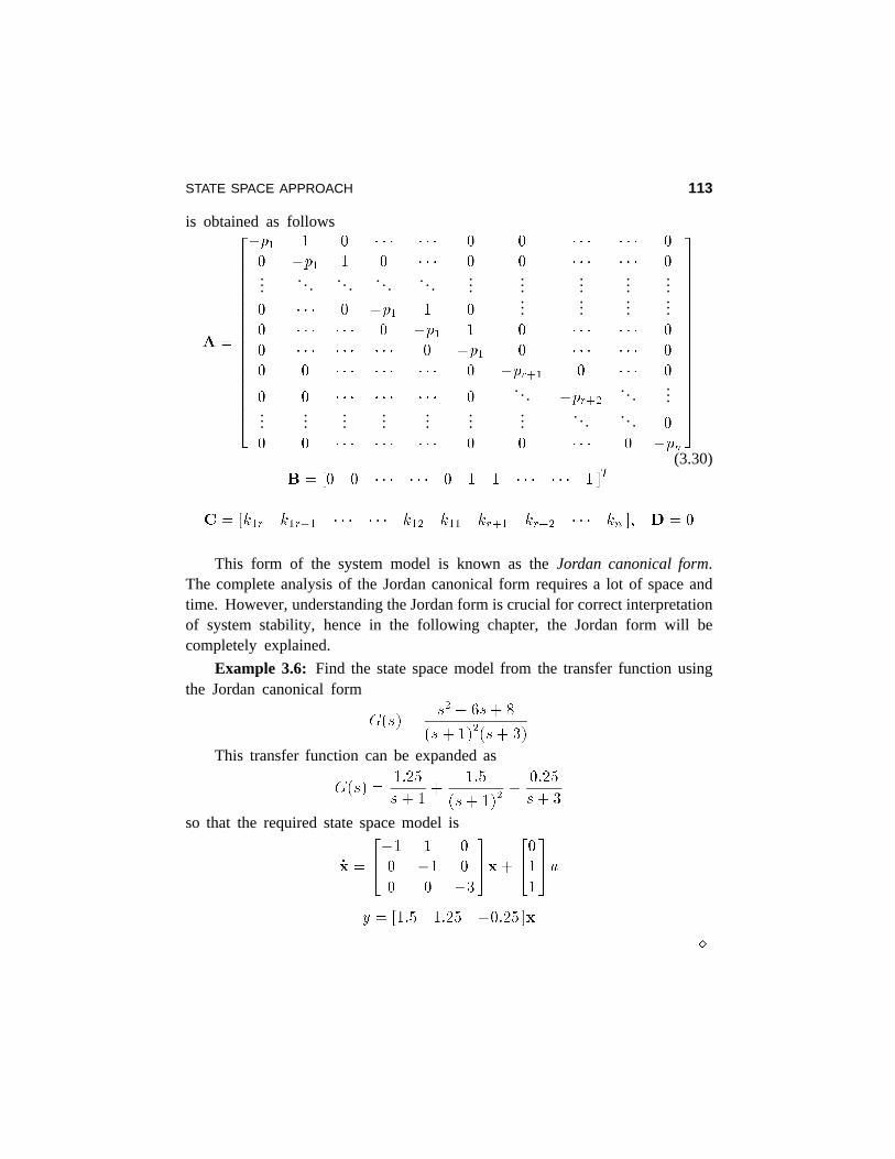
This form of the system model is known as theJordan canonical form.The complete analysis of the Jordan canonical form requires a lot of space andtime. However, understanding the Jordan form is crucial for correct interpretationof system stability, hence in the following chapter, the Jordan form will becompletely explained.
Example 3.6: Find the state space model from the transfer function usingthe Jordan canonical form
G(s) =s2 + 6s+ 8
(s+1)2(s+ 3)
This transfer function can be expanded as
G(s) =1:25
s + 1+
1:5
(s+1)2� 0:25
s +3
so that the required state space model is
_x =
24�1 1 0
0 �1 0
0 0 �3
35x+
24011
35uy = [1:5 1:25 �0:25 ]x
�
114 STATE SPACE APPROACH
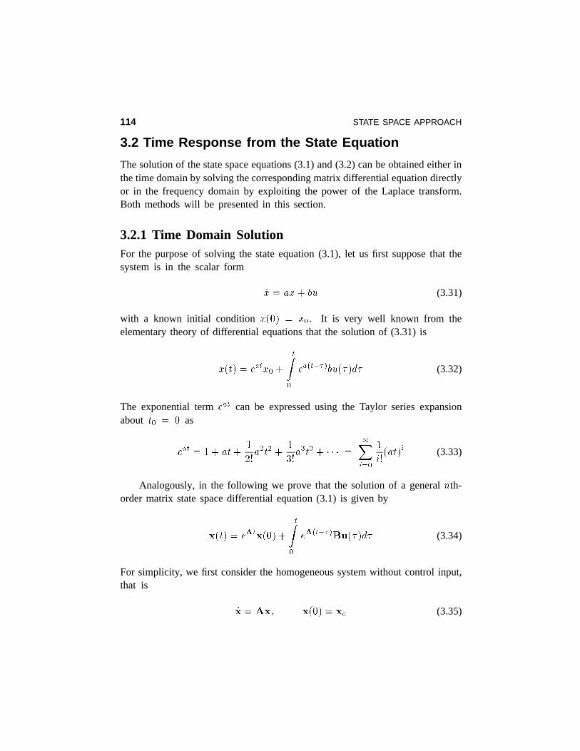
3.2 Time Response from the State Equation
The solution of the state space equations (3.1) and (3.2) can be obtained either inthe time domain by solving the corresponding matrix differential equation directlyor in the frequency domain by exploiting the power of the Laplace transform.Both methods will be presented in this section.
3.2.1 Time Domain SolutionFor the purpose of solving the state equation (3.1), let us first suppose that thesystem is in the scalar form
_x = ax+ bu (3.31)
with a known initial conditionx(0) = x0. It is very well known from theelementary theory of differential equations that the solution of (3.31) is
x(t) = eatx0 +
tZ0
ea(t��)bu(�)d� (3.32)
The exponential termeat can be expressed using the Taylor series expansionabout t0 = 0 as
eat = 1 + at+1
2!a2t2 +
1
3!a3t3 + � � � =
1Xi=0
1
i!(at)i (3.33)
Analogously, in the following we prove that the solution of a generalnth-order matrix state space differential equation (3.1) is given by
x(t) = eAtx(0) +
tZ0
eA(t��)Bu(�)d� (3.34)
For simplicity, we first consider the homogeneous system without control input,that is
_x = Ax; x(0) = x0 (3.35)
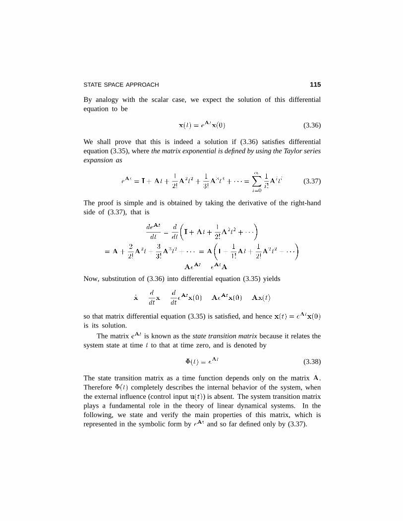
STATE SPACE APPROACH 115
By analogy with the scalar case, we expect the solution of this differentialequation to be
x(t) = eAtx(0) (3.36)
We shall prove that this is indeed a solution if (3.36) satisfies differentialequation (3.35), wherethe matrix exponential is defined by using the Taylor seriesexpansion as
eAt = I+At+1
2!A2t2 +
1
3!A3t3 + � � � =
1Xi=0
1
i!Aiti (3.37)
The proof is simple and is obtained by taking the derivative of the right-handside of (3.37), that is
deAt
dt=
d
dt
�I+At+
1
2!A2t2 + � � �
�=A+
2
2!A2t +
3
3!A3t2 + � � � =A
�I+
1
1!At+
1
2!A2t2 + � � �
�=AeAt = eAtA
Now, substitution of (3.36) into differential equation (3.35) yields
_x =d
dtx =
d
dteAtx(0) =AeAtx(0) = Ax(t)
so that matrix differential equation (3.35) is satisfied, and hencex(t) = eAtx(0)
is its solution.
The matrixeAt is known as thestate transition matrixbecause it relates thesystem state at timet to that at time zero, and is denoted by
�(t) = eAt (3.38)
The state transition matrix as a time function depends only on the matrixA.Therefore�(t) completely describes the internal behavior of the system, whenthe external influence (control inputu(t)) is absent. The system transition matrixplays a fundamental role in the theory of linear dynamical systems. In thefollowing, we state and verify the main properties of this matrix, which isrepresented in the symbolic form byeAt and so far defined only by (3.37).
116 STATE SPACE APPROACH
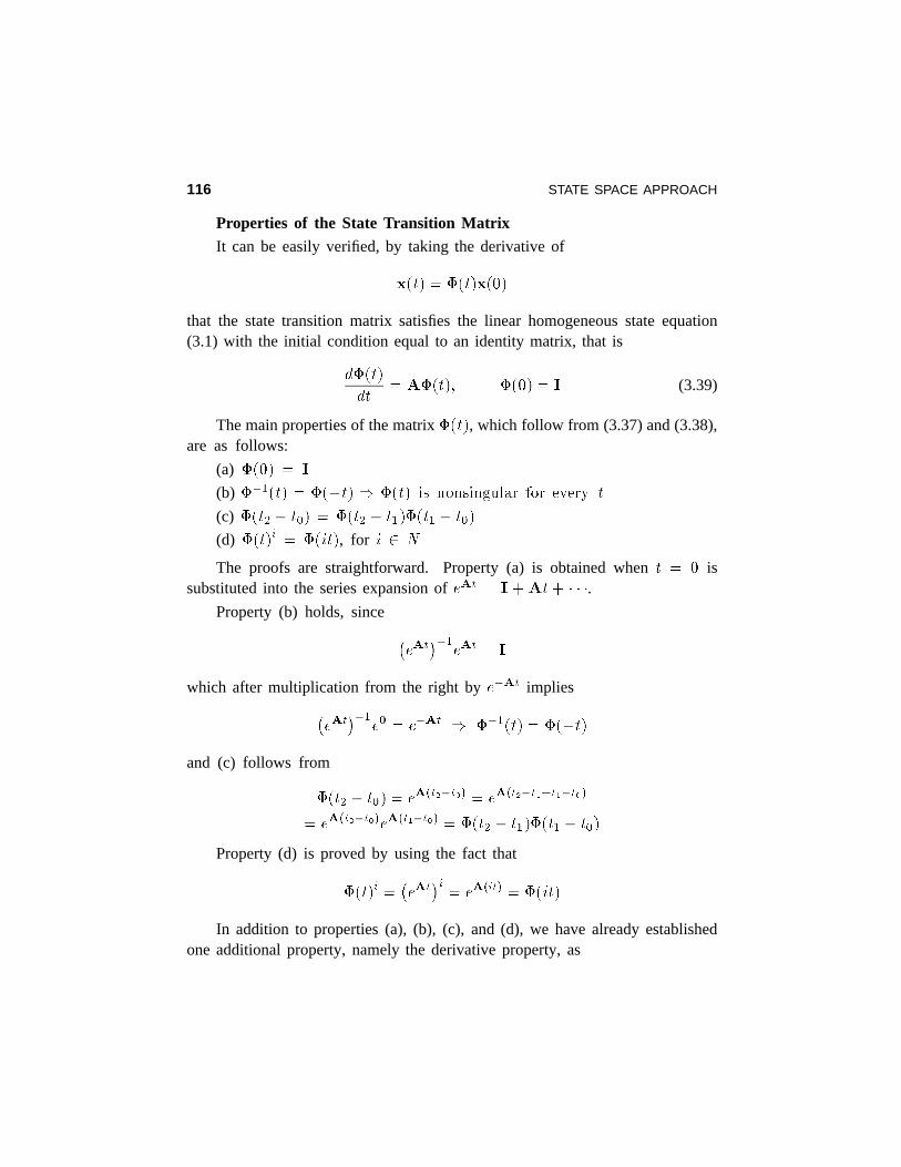
Properties of the State Transition Matrix
It can be easily verified, by taking the derivative of
x(t) = �(t)x(0)
that the state transition matrix satisfies the linear homogeneous state equation(3.1) with the initial condition equal to an identity matrix, that is
d�(t)
dt= A�(t); �(0) = I (3.39)
The main properties of the matrix�(t), which follow from (3.37) and (3.38),are as follows:
(a) �(0) = I
(b) ��1(t) = �(�t) ) �(t) is nonsingular for every t
(c) �(t2 � t0) = �(t2 � t1)�(t1 � t0)
(d) �(t)i = �(it), for i 2 N
The proofs are straightforward. Property (a) is obtained whent = 0 issubstituted into the series expansion ofeAt = I +At+ � � �.
Property (b) holds, since�eAt
��1eAt = I
which after multiplication from the right bye�At implies�eAt
��1e0 = e�At ) ��1(t) = �(�t)
and (c) follows from
�(t2 � t0) = eA(t2�t0) = eA(t2�t1+t1�t0)
= eA(t2�t0)eA(t1�t0) = �(t2 � t1)�(t1 � t0)
Property (d) is proved by using the fact that
�(t)i =�eAt
�i= eA(it) = �(it)
In addition to properties (a), (b), (c), and (d), we have already establishedone additional property, namely the derivative property, as
STATE SPACE APPROACH 117
(e)d
dt�(t) =A�(t) , d
dteAt = eAtA =AeAt
The state transition matrix�(t) can be found by using several methods. Twoof them are given in this chapter—formulas (3.37) and (3.49). The third one,very popular in linear algebra, is based on the Cayley–Hamilton theorem and isgiven in Appendix C.
In the case when the control vectoru(t) is present in the system (forcedresponse)
_x =Ax+Bu; x(0) = x0
we look for the solution of the state space equation in the form
x(t) = eAtf(t) (3.40)
Then_x(t) =AeAtf(t) + eAt _f(t) =Ax+ eAt _f (3.41)
It follows from (3.1) and (3.41) that
eAt _f(t) = Bu (3.42)
From (3.42) we have
_f (t) =�eAt
��1Bu =e�AtBu (3.43)
Integrating this equation, bearing in mind thatx(0) = eA�0f(0) = f(0), we get
f(t)� f(0) =tZ
0
e�A�Bu(�)d� (3.44)
Substitution of the last expression in (3.40) gives the required solution
x(t) = eAtx(0) +
tZ0
eA(t��)Bu(�)d� (3.45)
or
x(t) = �(t)x(0)+
tZ0
�(t� � )Bu(�)d� (3.46)
118 STATE SPACE APPROACH
When the initial state of the system is known at timet0, rather than at timet = 0,the solution of the state equation is similarly obtained as
x(t) = �(t� t0)x(t0) +
tZt0
�(t� �)Bu(�)d�
= eA(t�t0)x(t0) +
tZt0
eA(t��)Bu(�)d�
(3.47)
This can be easily verified by repeating steps (3.40)–(3.45) withx(t0) = x0 andx(t0) = eAt0f(t0).
Example 3.7: For the system given in Example 3.4 find the state transitionmatrix �(t). Evaluate�(1) using the MATLAB function expm. Assumingthatthe initial state of the system is zero, find the state response to a unit step. Checkthe solution obtained by using the MATLAB functionstep.
At the present time we are able to find the state transition matrix (matrixexponential) by using formula (3.37), which deals with an infinite series, andhence is not very convenient for calculations. Better ways to find�(t) are themethod based on the Cayley–Hamilton theorem (see Appendix C) and the formulabased on the Laplace transform, see formula (3.49). However, in this problem, ifwe start with the uncoupled (modal) state space form of the system considered inExample 3.4, we can avoid using any of the above methods in order to find thestate transition matrix. Namely,for diagonal matrices only, it is easy to show that
�(t) = e
24�1 0 0
0 �2 0
0 0 �3
35t
=
24e�t 0 0
0 e�2t 0
0 0 e�3t
35Using the MATLAB function for evaluating the matrix exponential asexpm(A*1), we get
�(1) =
24e�1 0 0
0 e�2 0
0 0 e�3
35 =
240:3679 0 0
0 0:1353 0
0 0 0:0498
35
STATE SPACE APPROACH 119
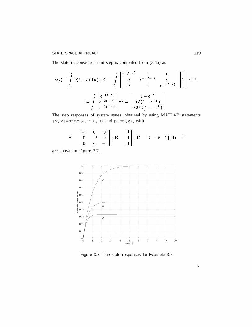
The state response to a unit step is computed from (3.46) as
x(t) =
tZ0
�(t � � )Bu(�)d� =
tZ0
24e�(t��) 0 0
0 e�2(t��) 0
0 0 e�3(t��)
3524111
35 � 1d�
=
tZ0
24 e�(t��)
e�2(t��)
e�3(t��)
35d� =
24 1� e�t
0:5�1� e�2t
�0:333
�1� e�3t
�35
The step responses of system states, obtained by using MATLAB statements[y,x]=step(A,B,C,D) andplot(x), with
A =
24�1 0 0
0 �2 0
0 0 �3
35; B =
24111
35; C = [6 �6 1 ]; D = 0
are shown in Figure 3.7.
0 1 2 3 4 5 6 7 8 9 100
0.1
0.2
0.3
0.4
0.5
0.6
0.7
0.8
0.9
1
time [s]
stat
e st
ep r
espo
nse
x3
x2
x1
Figure 3.7: The state responses for Example 3.7
�
120 STATE SPACE APPROACH
3.2.2 Solution Using the Laplace TransformThe time trajectory of the state vectorx(t) can be also found using the Laplacetransform method. The main properties of the Laplace transform and commontransform pairs are given in Appendix A.
The Laplace transform applied to the state equation (3.1) gives
sX(s)� x�0�� =AX(s) +BU(s)
orX(s) = (sI�A)�1x
�0�
�+ (sI�A)�1BU(s) (3.48)
Let us assume thatx(0) = x(0�). Comparing equations (3.46) and (3.48), itis easy to see that the term(sI�A)�1 is the Laplace transform of the statetransition matrix, that is
�(s) = (sI�A)�1 =1
det(sI�A)adj(sI�A) = Lf�(t)g (3.49)
The time form of the state vectorx(t) is obtained by applying the inverse Laplacetransform to
X(s) = �(s)x(0) +�(s)BU(s) (3.50)
Note that the second term on the right-hand side corresponds in the time domainto the convolution integral, so that we have
x(t) = eAtx(0) +
tZ0
eA(t��)Bu(�)d� (3.51)
Once the state vectorx(t) is determined, the output vectory(t) of the systemis simply obtained by substitution ofx(t) into equation (3.2), that is
y(t) = C�(t)x(0)+C
tZ0
�(t� �)Bu(�)d� +Du(t) (3.52)
or, in the complex domain
Y(s) = C�(s)x(0) + [C�(s)B+D]U(s) (3.53)
STATE SPACE APPROACH 121
3.2.3 State Space Model and Transfer Function
The matrix that establishes a relationship between the output vectorY(s) and theinput vectorU(s), for the zero initial conditions,x(0) = 0, is called thesystemmatrix transfer function. From (3.53) it is given by
G(s) = C(sI�A)�1B+D (3.54)
Note that (3.54) represents the open-loop system matrix transfer function.
Example 3.8: Find the transfer function for the system given in Example 3.4.
It is the easiest to use modal (uncoupled) canonical form, which leads to
G(s) = [6 �6 1 ]
24s+1 0 0
0 s+ 2 0
0 0 s+ 3
35�124111
35
= [6 �6 1 ]
24 1s+1 0 0
0 1s+2 0
0 0 1s+3
3524111
35=
6
s+ 1� 6
s + 2+
1
s +3=
(s+ 5)(s+4)
(s+ 1)(s+ 2)(s+3)
If we start with controller canonical form we will get, after some algebra,
G(s) = [20 9 1 ]
24s+ 6 �1 0
11 s �1
6 0 s
35�124001
35
= [20 9 1 ]1
s3 + 6s2 +11s+6
24s2 +6s+11 s + 6 1
�6 s(s+6) s
�6s �11s� 6 s2
3524001
35=
s2 + 9s+ 20
s3 + 6s2 + 11s+6
Note that the MATLAB functionss2tf can be used to solve the above problem.�
122 STATE SPACE APPROACH
3.3 Discrete-Time Models
Discrete-time systems are either inherently discrete (e.g. models of bank ac-counts, national economy growth models, population growth models, digitalwords) or they are obtained as a result of sampling (discretization) of continuous-time systems. In such kinds of systems, inputs, state space variables, and outputshave the discrete form and the system models can be represented in the formof transition tables.
The mathematical model of a discrete-time system can be written in termsof a recursive formula by using linear matrix difference equations as
x[(k + 1)T ] =Adx(kT ) +Bdu(kT )
y(kT ) = Cdx(kT ) +Ddu(kT )(3.55)
HereT represents the sampling interval, which may be omitted for brevity. Evenmore, in the case of inherent discrete systems, there is no need to introduce thenotion of the sampling intervalT so that these systems are described by (3.55)with T = 1.
Similarly to continuous-time systems, discrete state space equations canbe derived either from difference equations (Subsection 3.3.1) or from discretetransfer functions using simulation diagrams (Subsection 3.3.2). In Subsection3.3.3 we show how to discretize continuous-time linear systems and obtaindiscrete-time ones. In the rest of the section we parallel most of the resultsobtained in previous sections for continuous-time systems.
3.3.1 Difference Equations and State Space Form
An nth-orderdifference equation is given by
y(k+ n) + an�1y(k+ n� 1) + � � �+ a1y(k+ 1) + a0y(k)
= bnu(k+ n) + bn�1u(k+ n� 1) + � � �+ b1u(k+ 1) + b0u(k)(3.56)
This equation expresses all values in terms of discrete-timek.
The corresponding state space equation can be derived by using the sametechniques as in the continuous-time case. For example, for phase variable
STATE SPACE APPROACH 123
canonical form (controller canonical form) in discrete-time, we have2666664x1(k + 1)
x2(k + 1)...
xn�1(k +1)
xn(k+ 1)
3777775 =
2666640 1 0 � � � 0
0 0 1 � � � 0...
......
.. ....
0 0 0 � � � 1
�a0 �a1 �a2 � � � �an�1
3777752666664
x1(k)
x2(k)...
xn�1(k)xn(k)
3777775 +
2666640
0...0
1
377775u(k)
y(k) = [(b0 � a0bn) (b1 � a1bn) � � � (bn�1 � an�1bn) ]
2664x1(k)
x2(k)...
xn(k)
3775+ bnu(k)
(3.57)Note that the transformation equations, dual to the continuous-time ones(3.11)–(3.13), are given in the discrete-time domain by
�(k+ n) + an�1�(k + n � 1) + � � �+ a1�(k+ 1) + a0�(k) = u(k) (3.58)
x1(k) = �(k)
x2(k) = �(k+ 1)
x3(k) = �(k+ 2)
...
xn(k) = �(k + n � 1)
(3.59)
y(k) = b0�(k) + b1�(k+ 1) + b2�(k+ 2)+ � � �+ bn�(k+ n) (3.60)
Eliminating�(k+ n) from (3.60) by using (3.58) and (3.59), the output equationgiven in (3.57) is obtained.
3.3.2 Discrete Transfer Function and State Space ModelThe derivation of state space equations from discrete transfer functions, basedon simulation diagrams, is very similar to the continuous-time case. The onlydifference is that in simulation diagrams the integration block1=s is replaced bythe unit delay elementz�1. The state variables are selected as outputs of thesedelay elements. We shall illustrate this method by an example.
124 STATE SPACE APPROACH
Example 3.9: Find two state space forms for the transfer function
Y (z)
U(z)=
z +1:1
(z � 0:9)(z +0:7)(z � 0:7)
We solve this problem by using both direct (a) and parallel (b) programmingtechniques.
(a) The transfer function can be rewritten as
Y (z)
U(z)=
z +1:1
z3 � 0:9z2 � 0:49z +0:441
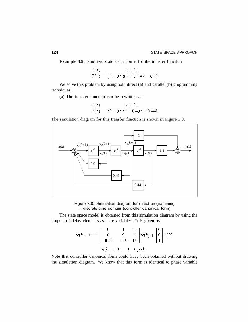
The simulation diagram for this transfer function is shown in Figure 3.8.
x1(k+1)
x1(k)
x2(k+1)
x2(k)x3(k)
x3(k+1)
0.9
z-1 ΣΣu(k) y(k)
z-1 z-1
1
1.1
-0.441
0.49
Figure 3.8: Simulation diagram for direct programmingin discrete-time domain (controller canonical form)
The state space model is obtained from this simulation diagram by using theoutputsof delay elements as state variables. It is given by
x(k + 1) =
24 0 1 0
0 0 1
�0:441 0:49 0:9
35x(k) +24001
35u(k)y(k) = [1:1 1 0 ]x(k)
Note that controller canonical form could have been obtained without drawingthe simulation diagram. We know that this form is identical to phase variable
STATE SPACE APPROACH 125
canonical form, which is represented by (3.57). Identifying the correspondingcoefficients in the original transfer function, the desired state space form isobtained directly from (3.57). We have used the above method in order todemonstrate at the same time the procedure of drawing simulation diagrams inthe discrete-time domain.
(b) Employing the partial fraction expansion (with help of the MATLABfunction residue), we get
Y (z)
U(z)=
6:25
z � 0:9+
0:1786
z + 0:7+�6:4286
z � 0:7
Since the poles of the transfer function are real and distinct we get the modalcanonical form as
x(k + 1) =
240:9 0 0
0 �0:7 0
0 0 0:7
35x(k) +24111
35u(k)y(k) = [6:25 0:1786 �6:4286]x(k)
�
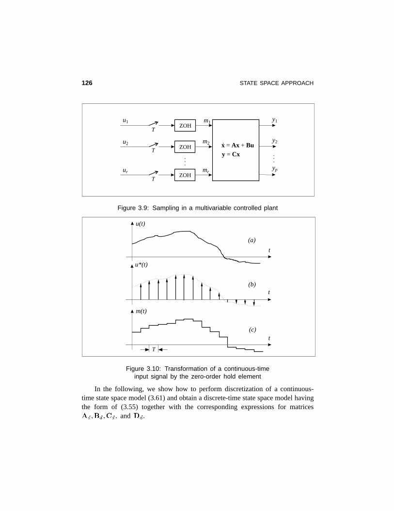
3.3.3 Discretization of Continuous-Time SystemsReal physical dynamic systems are continuous in nature. In this section, weshow how to obtain discrete-time state space models from continuous-time systemmodels. Assume that the plant is linear, continuous, and time invariant withr-inputs andp-outputs (see Figure 3.9). Inputs are sampled by using the zero-orderhold (ZOH) device. This device samples inputs at discrete-time instantskT (seeFigure 3.10b) and the values obtained for vectoru(kT ) are held until(k+ 1)T .The corresponding signal is given in Figure 3.10c.
The state space model of such a plant is
_x(t) =Ax(t) +Bm(t)
y(t) = Cx(t) +Dm(t)(3.61)
These equations define states and outputs during the sampling intervalkT � t < (k +1)T . Input signalsmi(t); i = 1; :::; r; are defined by
mi(t) = mi(kT ) = ui(kT ); kT � t < (k+ 1)T; k = 0; 1; 2; ::: (3.62)
126 STATE SPACE APPROACH
x = Ax + Buy = Cx
.
ZOH
ZOH
ZOH
m1
m2
mr
u1
u2
ur
T
T
T
y1
y2
yp... .
..
Figure 3.9: Sampling in a multivariable controlled plant
u(t)
m(t)
T
(a)
(b)
(c)
t
t
t
u*(t)
Figure 3.10: Transformation of a continuous-timeinput signal by the zero-order hold element
In the following, we show how to perform discretization of a continuous-time state space model (3.61) and obtain a discrete-time state space model havingthe form of (3.55) together with the corresponding expressions for matricesAd;Bd;Cd; andDd.
STATE SPACE APPROACH 127
Consider formula (3.45) witht = T
x(T ) = eATx(0) +
TZ0
eA(T��)Bu(0)d�
= eATx(0) + eATTZ0
e�A�d�Bu(0) = �(T )x(0) +
TZ0
�(T � �)d�Bu(0)
(3.63)which can be written in the form
x(T ) =Adx(0) +Bdu(0) (3.64)
Comparing (3.63) and (3.64) we can find expressions forAd andBd. They aregiven by
Ad = eAT = �(T )
Bd = eATTZ0
e�A�d�B =
TZ0
eA(T��)d� �B =
TZ0
eA�d� �B(3.65)
Note thatAd andBd are obtained for the time interval from0 to T . However,it can easily be shown that due to system time invariance the same expressionsfor Ad andBd are obtained for any time interval. Namely, steps (3.63)–(3.65)can be repeated for succeeding time intervals2T; 3T; :::; (k + 1)T with initialconditions taken, respectively, asx(T );x(2T); :::;x(kT ). Therefore, for the timeinstantt = (k+ 1)T and for t0 = kT , we have from (3.47)
x[(k+ 1)T ] = �[(k+ 1)T � kT ]x(kT ) +
(k+1)TZkT
�[(k+ 1)T � � ]d�Bu(kT )
=Adx(kT ) +Bdu(kT )(3.66)
From the above equation we see that the matricesAd andBd are given by
Ad = �[(k+ 1)T � kT ] = �(T ) = eAT
Bd =
(k+1)TZkT
�[(k +1)T � � ]d�B =
TZ0
�(�)d�B =
TZ0
eA�d�B(3.67)
128 STATE SPACE APPROACH
The last equality is obtained by using change of variables as� = (k +1)T � � .Since (3.65) and (3.67) are identical, we conclude that for a time invariantcontinuous-time linear system, the discretization procedure yields a time invariantdiscrete-time linear system whose matricesAd andBd depend only onA, B,and the sampling intervalT .
In a similar manner the output equation (3.61) att = kT is given by
y(kT ) = Cx(kT ) +Du(kT ) (3.68)
Comparing this equation with the general output equation of linear discrete-timesystems (3.55), we conclude that
Cd = C; Dd = D (3.69)
In the literature one can find several methods for discretization of continuous-time linear systems. The discretization technique presented in this section isknown as theintegral approximation method.
In the case of discrete-time linear systems obtained by sampling continuous-time linear systems, the matrixAd, given by (3.65), can be determined fromthe infinite series
Ad = eAT = I+AT +1
2!A2T 2 + � � � =
1Xi=0
1
i!AiT i (3.70)
It can be also obtained either by using formula (3.49) or the method based onthe Cayley–Hamilton theorem and settingt = T in �(t) = eAt. Also, in orderto evaluateeAT we can use MATLAB functionexpm(A*T).
To find Bd, the second expression in (3.65) is integrated to give (seeAppendix C—matrix integrals)
Bd = eAT��e�ATA�1 +A�1
�B = (Ad � I)A�1B (3.71)
which is valid under the assumption thatA is invertible. If A is singular,Bd
can be determined from
Bd =
1Xi=1
T i
i!Ai�1
!B =
1Xi=0
T i+1
(i+1)!Ai
!B (3.72)
STATE SPACE APPROACH 129
which is obtained by using (3.37) in (3.67) and performing the correspondingintegration. Note that the above sum converges quite quickly so that only a fewterms give quite an accurate expression forBd.
Example 3.10: Find the discrete-time state space model of a continuous-time system
_x =
�0 1
�2 �3�x+
�0
1
�u
y = [1 0 ]x
The sampling periodT is equal to0:1.
According to (3.65) and (3.69), we have from (3.49)
Ad = �(T ) =
�2e�T � e�2T e�T � e�2T
2e�2T � 2e�T 2e�2T � e�T
�=
�0:9909 0:0861
�0:1722 0:7326
�
Bd = (Ad � I)A�1B =
�12
�1 + e�2T
�� e�T
e�T � e�2T
�=
�0:0045
0:0861
�Cd = [1 0 ]; Dd = 0
The same result is obtained by using the MATLAB function for discretization ofa continuous state space model as[Ad,Bd]=c2d(A,B,T).
�
3.3.4 Solution of the Discrete-Time State EquationThe objective of this section is to find the solution of the difference state equation(3.55) for the given initial statex(0) and the control signalu(k) at the samplinginstantsT; 2T;:::; kT . For simplicity we assumeT = 1.
From the state equationx(k+ 1) = Adx(k) + Bdu(k), for k = 0; 1; :::;
N � 1, it follows
x(1) =Adx(0) +Bdu(0)
x(2) =Adx(1) +Bdu(1) =A2dx(0) +AdBdu(0) + Bdu(1)
x(3) =Adx(2) +Bdu(2) =A3dx(0) +A
2dBdu(0) +AdBdu(1) +Bdu(2)
130 STATE SPACE APPROACH
...
x(N) =Adx(N � 1) +Bdu(N � 1) = ANd x(0) +
N�1Xi=0
AN�i�1d Bdu(i)
(3.73)
Using the notion of thediscrete-timestate transition matrixdefined by
�d(k) =Akd (3.74)
we get
x(N) = �d(N)x(0) +N�1Xi=0
�d(N � i� 1)Bdu(i) (3.75)
Note that the discrete-time state transition matrix relates the state of an input-free system at initial time (k = 0) to the state of the system at any other timek > 0, that is
x(k) = �d(k)x(0) = Akdx(0) (3.76)
It is easy to verify that the discrete-time state transition matrix has thefollowing properties
(a) �d(0) = A0d = I ( x(0) = �d(0)x(0)
(b) �d(k2 � k0) = �d(k2 � k1)�d(k1 � k0) = Ak2�k1d Ak1�k0
d =Ak2�k0d
(c) �id(k) = �d(ik) (
�Ak
d
�i= Aik
d
(d) �d(k+ 1) = Ad�d(k); �d(0) = I
The last property follows from
x(k +1) =Adx(k) ) �d(k+ 1)x(0) =Ad�d(k)x(0)
It is important to point out that the discrete-time state transition matrix maybe singular, which follows from the fact thatAk
d is nonsingular if and only ifthe matrixAd is nonsingular. In the case of inherent discrete-time systems, thematrixAd may be singular in general. However, ifAd is obtained through thediscretization procedure of a continuous-time linear system, like in (3.65), then
(Ad)�1 =
�eAT
��1= e�AT
so that the discrete-time state transition matrix is nonsingular in this case.
STATE SPACE APPROACH 131
Remark 1: If the initial value of the state vector is notx(0) but x(k0),then the solution (3.75) is
x(k0 +N) = �d(N)x(k0) +N�1Xi=0
�d(N � i� 1)Bdu(k0 + i) (3.77)
The output of the system at sampling instantk = N is obtained by substi-tuting x(k) from (3.75) into the output equation, producing
y(N) = Cd�d(N)x(0) +Cd
N�1Xi=0
�(N � i� 1)Bdu(i) +Ddu(N) (3.78)
Note that forT 6= 1, equations (3.75) and (3.78) are modified as
x(NT ) = �d(NT )x(0) +N�1Xi=0
�d[(N � i� 1)T ]Bdu(iT ) (3.79)
y(NT ) = Cd�d(NT )x(0) +Cd
N�1Xi=0
�[(N � i� 1)T ]Bdu(iT ) +Ddu(NT)
(3.80)
Remark 2: The discrete-time state transition matrix defined byAkd can
be evaluated efficiently for large values ofk by using a method based on theCayley–Hamilton theorem and described in Appendix C. It can be also evaluatedby using theZ-transformmethod as given in formula (3.85), see Subsection 3.3.5.
Example 3.11: For the system given in Example 3.10, use MATLAB tofind the unit step and impulse responses assuming that the initial condition isx(0) = [0 0 ]T .
The required time responses can be obtained directly by using MAT-LAB statements[y,x]=dstep(Ad,Bd,Cd,Dd) (for step response) and[y,x]=dimpulse(Ad,Bd,Cd,Dd) (for impulse response) with the discrete-
132 STATE SPACE APPROACH
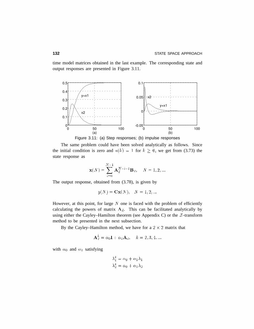
time model matrices obtained in the last example. The corresponding state andoutput responses are presented in Figure 3.11.
0 50 1000
0.1
0.2
0.3
0.4
0.5
(a)
x2
y=x1
0 50 100-0.05
0
0.05
0.1
(b)
y=x1
x2
Figure 3.11: (a) Step responses; (b) impulse responses
The same problem could have been solved analytically as follows. Sincethe initial condition is zero andu(k) = 1 for k � 0, we get from (3.73) thestate response as
x(N) =N�1Xi=0
AN�i�1d Bd; N = 1;2; :::
The output response, obtained from (3.78), is given by
y(N) = Cx(N); N = 1; 2; :::
However, at this point, for largeN one is faced with the problem of efficientlycalculating the powers of matrixAd. This can be facilitated analytically byusing either the Cayley–Hamilton theorem (see Appendix C) or theZ-transformmethodto be presented in the next subsection.
By the Cayley–Hamilton method, we have for a2 � 2 matrix that
Akd = �0I+ �1Ad; k = 2;3;4; :::
with �0 and �1 satisfying
�k1 = �0 + �1�1
�k2 = �0 + �1�2
STATE SPACE APPROACH 133
where�1 and �2 are distinct eigenvalues ofAd. System eigenvalues will beconsidered in Section 3.4.
�
3.3.5 Solution of the Discrete State Equation bythe Z-transform
Applying the Z-transform (see Appendix B) to the state space equation of adiscrete-time system
x(k + 1) =Adx(k) +Bdu(k) (3.81)
we get
zX(z)� zx(0) =AdX(z) +BdU(z) (3.82)
The complex state vectorX(z) can be expressed as
X(z) = (zI�Ad)�1zx(0) + (zI�Ad)
�1BdU(z) (3.83)
The inversez-transform of the last equation givesx(k), that is
x(k) = Z�1h(zI�Ad)
�1zix(0) +Z�1
h(zI�Ad)
�1BdU(z)i
(3.84)
Comparing equations (3.75) and (3.84) we conclude that
�d(k) = Z�1h(zI�Ad)
�1zi=Ak
d; k = 1;2;3; ::: (3.85)
Let us repeat and emphasize that the discrete state transition matrix�d(k) ofa general discrete-time invariant linear system can be obtained either by using(3.85) or the Cayley–Hamilton method given in Appendix C.
The inverse transform of the second term on the right-hand side of (3.84)is obtained directly by the application of the discrete convolution theorem (seeAppendix B), leading to
Z�1n(zI�Ad)
�1BdU(z)o=
k�1Xi=0
�d(k� 1� i)Bdu(i) (3.86)
134 STATE SPACE APPROACH
Combining (3.84) and (3.86) we get the required solution of the discrete-timestate space equation as
x(k) = �d(k)x(0) +k�1Xi=0
�d(k � i� 1)Bdu(i) (3.87)
The complex form of the output vectorY(z) is obtained if theZ-transformis applied to the output equation
y(k) = Cdx(k) +Ddu(k)
andX(z) is substituted from (3.83), leading to
Y(z) = Cd(zI�Ad)�1zx(0) +
hCd(zI�Ad)
�1Bd +Dd
iU(z)
From the above expression, for the zero initial condition, i.e.x(0) = 0, thediscrete matrix transfer functionis given by
Gd(z) = Cd(zI�Ad)�1Bd +Dd (3.88)
3.3.6 Response Between Sampling InstantsAn important feature of the state variable method is that it can be modified todetermine the output between sampling instants. Lett0 = kT andt = (k+�)T ,where0 � � < 1. Equation (3.47) gives
x[(k+�)T ] = eA�Tx(kT ) +
(k+�)TZkT
eA[(k+�)T�� ]Bu(�)d� (3.89)
Replacing (k+�)T � � by � and assuming thatu(�) is constant duringkT � � < (k+�)T , we get
x[(k +�)T ] = eA�Tx(kT ) +
�TZ0
eA�d�Bu(kT)
=Ad(�T )x(kT ) +Bd(�T )u(kT )
(3.90)
whereAd(�T ) = eA�T (3.91)
STATE SPACE APPROACH 135
and
Bd(�T ) =
�TZ0
eA�d�B (3.92)
Therefore, the matrixAd(�T ) is obtained by replacingT by �T in Ad.Similarly, Bd(�T ) is obtained by replacingT by �T in Bd.
3.3.7 Euler’s Approximation
Discretization of a continuous-time linear model, as presented in Subsection 3.3.3,by the integral approximation method, gives a desired discrete-time linear model.However, in the case of high-order systems, computation of the state transitionmatrix is very involved, so that in those cases the matricesAd and Bd arecalculated approximately by using some simpler methods. The simplest such amethod, known as Euler’s approximation, is just one of several methods used fornumerical solution of differential equations.
The objective of numerical integration is to find a discrete-time counterpartto a continuous-time model
_x(t) =Ax(t) +Bm(t)
in the form of a difference equation. The equation obtained, given by a recursiveformula, is then easily solved by a digital computer. The integration of theabove equation gives
x(t) =
tZ�1
[Ax(�) +Bm(�)]d�
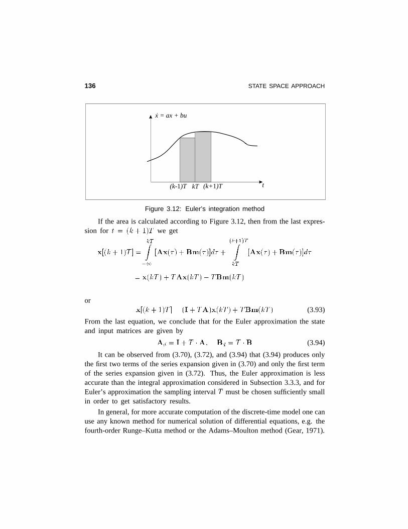
For simplicity, the main idea of the Euler method is explained for a scalarcase. Consider the first-order system_x = ax+bu. The integration is analogous tothe problem of finding the area, within the imposed integration limits, betweenthe curve defined byf(t) = ax(t) + bu(t) and the time axis. This area isapproximately equal to the sum of the rectangles in Figure 3.12.
136 STATE SPACE APPROACH
kT (k+1)T(k-1)T t
x = ax + bu.
Figure 3.12: Euler’s integration method
If the area is calculated according to Figure 3.12, then from the last expres-sion for t = (k + 1)T we get
x[(k+ 1)T ] =
kTZ�1
[Ax(�) +Bm(�)]d� +
(k+1)TZkT
[Ax(�) +Bm(�)]d�
= x(kT ) + TAx(kT) + TBm(kT)
orx[(k +1)T ] = (I+ TA)x(kT) + TBm(kT) (3.93)
From the last equation, we conclude that for the Euler approximation the stateand input matrices are given by
Ad = I+ T �A; Bd = T �B (3.94)
It can be observed from (3.70), (3.72), and (3.94) that (3.94) produces onlythe first two terms of the series expansion given in (3.70) and only the first termof the series expansion given in (3.72). Thus, the Euler approximation is lessaccurate than the integral approximation considered in Subsection 3.3.3, and forEuler’s approximation the sampling intervalT must be chosen sufficiently smallin order to get satisfactory results.
In general, for more accurate computation of the discrete-time model one canuse any known method for numerical solution of differential equations, e.g. thefourth-orderRunge–Kutta method or the Adams–Moulton method (Gear, 1971).
STATE SPACE APPROACH 137
3.4 The System Characteristic Equation andEigenvalues
The characteristic equation is very important in the study of both linear timeinvariant continuous and discrete systems. No matter what model type is consid-ered (ordinarynth-order differential equation, state space or transfer function),the characteristic equation always has the same form.
If we start with a differentialnth-order system model in the operator form�pn + an�1pn�1 + � � �+ a1p+ a0
�y(t)
=�bmp
m + bm�1pm�1 + � � �+ b1p+ b0�u(t)
where the operatorp is defined as
pi =di
dti; i = 1;2; . . . ; n� 1
and m � n, then thecharacteristicequation, according to the mathematicaltheory of linear differential equations (Boyce and DiPrima, 1992), is defined by
sn + an�1sn�1 + � � �+ a1s+ a0 = 0 (3.95)
Note that the operatorp is replaced by the complex variables playing the roleof a derivative in the Laplace transform context.
In the state space variable approach we have seen from (3.54) that
G(s) = C(sI�A)�1B+D =1
jsI�AjC[adj(sI�A)]B+D
=1
jsI�AjfC[adj(sI�A)]B+ jsI�AjDg
The characteristic equation here is defined by
jsI�Aj = 0 (3.96)
A third form of the characteristic equation is obtained in the context of thetransfer function approach. The transfer function of a single-input single-outputsystem is
G(s) =bms
m + bm�1sm�1 + � � �+ b1s+ b0sn + an�1sn�1 + � � �+ a1s+ a0
(3.97)
138 STATE SPACE APPROACH
The characteristic equation in this case is obtained by equating the denominatorof this expression to zero. Note that for multivariable systems, the characteristicpolynomial (obtained from the corresponding characteristic equation) appears indenominators of all entries of the matrix transfer function.
No matter what form of the system model is considered, the characteristicequation is always the same. This is obvious from (3.95) and (3.97), but is notso clear from (3.96). It is left as an exercise to the reader to show that (3.95)and (3.96) are identical (Problem 3.30).
The eigenvaluesare defined in linear algebra as scalars,�, satisfying(Fraleigh and Beauregard, 1990)
Av = �v (3.98)
where the vectorsv 6= 0 are called theeigenvectors. This system ofn linearalgebraic equations (� is fixed) has a solutionv 6= 0 if and only if
j�I�Aj = 0 (3.99)
Obviously, (3.96) and (3.99) have the same form. Since (3.96) = (3.95), it followsthat the last equation is the characteristic equation, and hence the eigenvalues arethe zeros of the characteristic equation. For the characteristic equation of ordern, the number of eigenvalues is equal ton. Thus, the roots of the characteristicequation in the state space context are the eigenvalues of the matrixA. Theseroots in the transfer function context are called thesystem poles, according to themathematical tools for analysis of these systems—the complex variable methods.
Similarity Transformation
We have pointed out before that a system modeled by the state spacetechnique may have many state space forms. Here, we establish a relationshipamong those state space forms by using a linear transformation known as thesimilarity transformation.
For a given system
_x =Ax+Bu; x(0) = x0
y = Cx+Du
we can introduce a new state vectorx by a linear coordinate transformation asfollows
x = Px
STATE SPACE APPROACH 139
whereP is some nonsingularn�n matrix. A new state space model is obtained as
_x = Ax+ Bu; x(0) = x0
y = Cx+ Du(3.100)
where
A = P�1AP; B = P�1B; C = CP; D =D; x(0) = P�1x(0) (3.101)
This transformation is known in the literature as thesimilarity transformation.Itplays an important role in linear control system theory and practice.
Very important features of this transformation are that under similaritytransformation both the system eigenvalues and the system transfer function areinvariant.
Eigenvalue Invariance
A new state space model obtained by the similarity transformation does notchange internal structure of the model, that is, the eigenvalues of the systemremain the same. This can be shown as follows���sI� A��� = ��sI�P�1AP�� = ��P�1(sI�A)P
��=
��P�1��jsI�AjjPj = jsI�Aj(3.102)
Note that in this proof the following properties of the matrix determinant havebeen used
det(M1M2M3) = detM1�detM2�detM3
detM�1 =1
detM
see Appendix C.
Transfer Function Invariance
Another important feature of the similarity transformation is that the transferfunction remains the same for both models, which can be shown as follows
G(s) = C�sI� A
��1B+ D = CP
�sI�P�1AP��1P�1B+D
= CP�P�1(sI�A)P
��1P�1B+D
= CPP�1(sI�A)�1PP�1B+D
= C(sI�A)�1B+D =G(s)
(3.103)
140 STATE SPACE APPROACH
Note that we have used in (3.103) the matrix inversion property (Appendix C)
(M1M2M3)�1 =M�1
3 M�12 M
�11
The above result is quite logical—the system preserves its input–output behaviorno matter how it is mathematically described.
Modal Transformation
One of the most interesting similarity transformations is the one that putsmatrixA into diagonal form. Assume thatP = V = [v1;v2; . . . ;vn], whereviare the eigenvectors. We then have
V�1AV = A = � = diag(�1; �2; . . . ; �n) (3.104)
It is easy to show that the elements�i; i = 1; :::;n, on the matrix diagonal of� are the roots of the characteristic equationjsI� �j = jsI�Aj = 0, i.e. theyare the eigenvalues. This can be shown in a straightforward way
jsI� �j = detfdiag(s� �1; s� �2; . . . ; s� �n)g= (s� �1)(s� �2) � � � (s� �n)
The state transformation (3.104) is known as themodal transformation.
Note that the pure diagonal state space form defined in (3.104) can beobtained only in the following three cases.
1. The system matrix has distinct eigenvalues, namely�1 6= �2 6= � � � 6= �n.2. The system matrix is symmetric (see Appendix C).3. The system minimal polynomial does not contain multiple eigenvalues.
For the definition of the minimal polynomial and the corresponding purediagonal Jordan form, see Subsection 4.2.4.
In the above three cases we say that the system matrix is diagonalizable.
Remark: Relation (3.104) may be represented in another form, that is
V�1A = �V�1
orWTA = �WT
whereWT =V�1 ) WTV = I
STATE SPACE APPROACH 141
In this case theleft eigenvectorswi; i = 1;2; :::; n; can be computed from
wTi A = �iw
Ti ) ATwi = �iwi
whereW = [w1;w2; . . . ;wn]. Since j�I�Aj = ���I�AT��, then�i is also
an eigenvalue ofAT .
There are numerous program packages available to compute both the eigen-values and eigenvectors of a matrix. In MATLAB this is done by using thefunction eig.
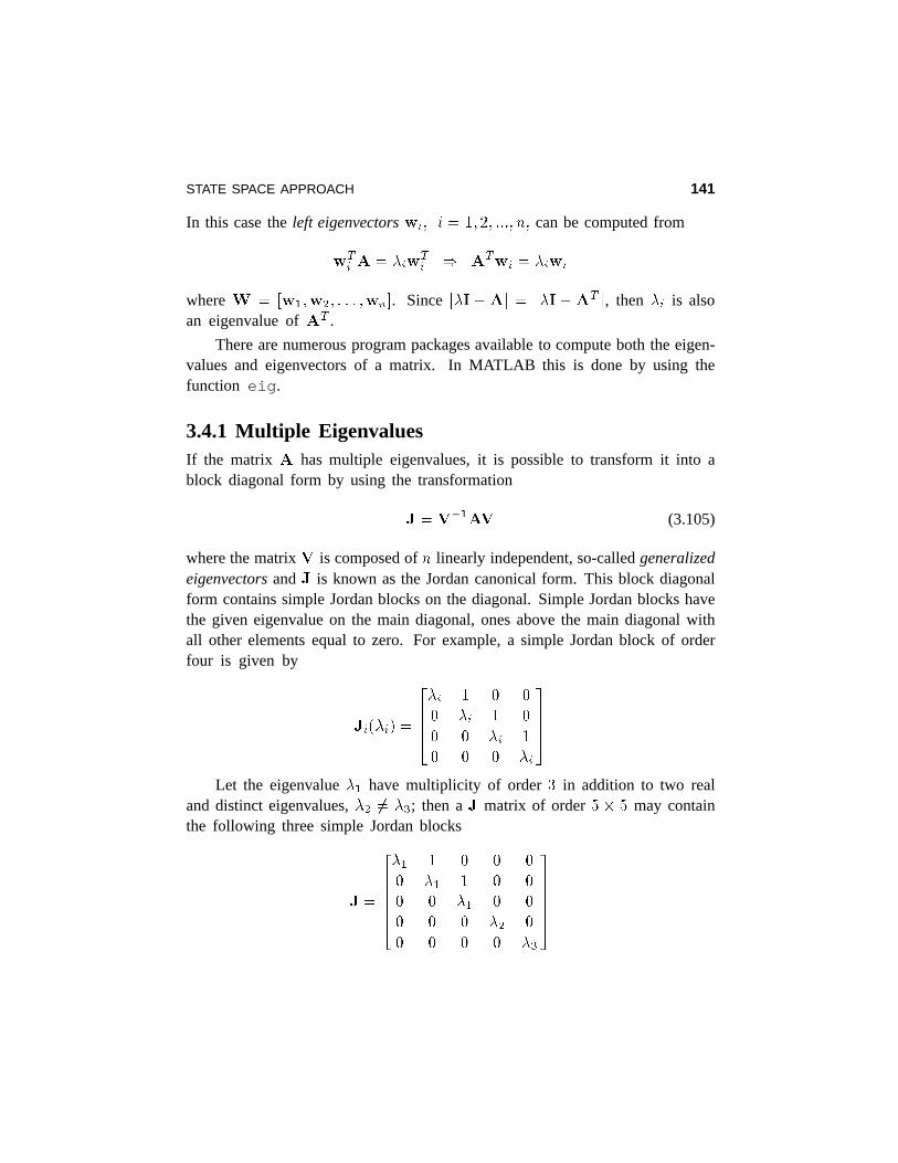
3.4.1 Multiple EigenvaluesIf the matrix A has multiple eigenvalues, it is possible to transform it into ablock diagonal form by using the transformation
J =V�1AV (3.105)
where the matrixV is composed ofn linearly independent, so-calledgeneralizedeigenvectorsandJ is known as the Jordan canonical form. This block diagonalform contains simple Jordan blocks on the diagonal. Simple Jordan blocks havethe given eigenvalue on the main diagonal, ones above the main diagonal withall other elements equal to zero. For example, a simple Jordan block of orderfour is given by
Ji(�i) =
2664�i 1 0 0
0 �i 1 0
0 0 �i 1
0 0 0 �i
3775Let the eigenvalue�1 have multiplicity of order3 in addition to two real
and distinct eigenvalues,�2 6= �3; then aJ matrix of order5 � 5 may containthe following three simple Jordan blocks
J =
266664�1 1 0 0 0
0 �1 1 0 0
0 0 �1 0 0
0 0 0 �2 0
0 0 0 0 �3
377775
142 STATE SPACE APPROACH
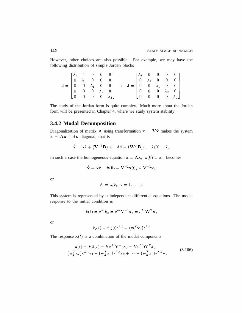
However, other choices are also possible. For example, we may have thefollowing distribution of simple Jordan blocks
J =
266664�1 1 0 0 0
0 �1 0 0 0
0 0 �1 0 0
0 0 0 �2 0
0 0 0 0 �3
377775 or J =
266664�1 0 0 0 0
0 �1 0 0 0
0 0 �1 0 0
0 0 0 �2 0
0 0 0 0 �3
377775The study of the Jordan form is quite complex. Much more about the Jordanform will be presented in Chapter 4, where we study system stability.
3.4.2 Modal DecompositionDiagonalization of matrixA using transformationx = Vx makes the system_x = Ax + Bu diagonal, that is
_x = �x+�V�1B
�u = �x+
�WTB
�u; x(0) = x0
In such a case the homogeneous equation_x = Ax; x(0) = x0, becomes
_x = �x; x(0) =V�1x(0) =V�1x0
or_xi = �ixi; i = 1; . . . ; n
This system is represented byn independent differential equations. The modalresponse to the initial condition is
x(t) = e�tx0 = e�tV�1x0 = e�tWTx0
orxi(t) = xi(0)e
�it =�wT
i x0�e�it
The responsex(t) is a combination of the modal components
x(t) =Vx(t) =Ve�tV�1x0 =Ve�tWTx0
=�wT1 x0
�e�1tv1 +
�wT2 x0
�e�2tv2 + � � �+ �
wTnx0
�e�ntvn
(3.106)
STATE SPACE APPROACH 143
This equation represents the modal decomposition ofx(t) and it shows that thetotal response consists of a sum of responses of all individual modes. Note thatwTi x0 are scalars.
It is customary to call the reciprocals of�i the systemtime constantsanddenote them by�i, that is
�i =1
�i; i = 1;2; :::;n
This has physical meaning since the system dynamics is determined by its timeconstants and these do appear in the system response in the forme�t=�i .
The transient response of the system may be influenced differently bydifferent modes, depending of the eigenvalues�i. Some modes may decay fasterthan the others. Some modes might be dominant in the system response. Thesecases will be illustrated in Chapter 6.
Remark: A similarity transformation� = V�1AV can be used for thestate transition matrix calculation. Recall
x(t) = e�tx(0); x(t) =Vx(t); x(0) =Vx(0)
and
x(t) =V�1e�tVx(0) = �(t)x(0)
Hence,
�(t) = e�t =V�1e�tV =WTe�tV
or, in the complex domain
�(s) = V�1(sI� �)�1V
=V�1diagfs� �1; s� �2; . . . ; s� �ng�1V
= V�1diag�
1
s � �1;
1
s � �2; . . . ;
1
s � �n
�V
Remark: The presented theory about the system characteristic equation,eigenvalues, eigenvectors, similarity and modal transformations can be applieddirectly to discrete-time linear systems withAd replacingA.
144 STATE SPACE APPROACH
3.5 State Space MATLAB Laboratory ExperimentsIn this section we present three MATLAB laboratory experiments on the statespace method in control systems. These experiments can be used either as sup-plements for lectures or independently in the corresponding control system lab-oratory. Most of the required MATLAB functions have been already introducedin the examples done in this chapter. Students should also consult AppendixD, where a shortened MATLAB manual is given. It is advisable that beforeusing any MATLAB function, the students check all its options by typinghelpfunction name.
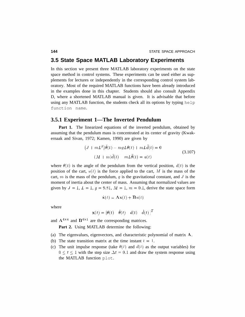
3.5.1 Experiment 1—The Inverted PendulumPart 1. The linearized equations of the inverted pendulum, obtained by
assuming that the pendulum mass is concentrated at its center of gravity (Kwak-ernaak and Sivan, 1972; Kamen, 1990) are given by�
J +mL2���(t)�mgL�(t) +mL �d(t) = 0
(M +m) �d(t) +mL��(t) = u(t)(3.107)
where�(t) is the angle of the pendulum from the vertical position,d(t) is theposition of the cart,u(t) is the force applied to the cart,M is the mass of thecart,m is the mass of the pendulum,g is the gravitational constant, andJ is themoment of inertia about the center of mass. Assuming that normalized values aregiven byJ = 1, L = 1, g = 9:81, M = 1, m = 0:1, derive the state space form
_x(t) =Ax(t) +Bu(t)
wherex(t) = [�(t) _�(t) d(t) _d(t) ]T
andA4�4 andB4�1 are the corresponding matrices.
Part 2. Using MATLAB determine the following:
(a) The eigenvalues, eigenvectors, and characteristic polynomial of matrixA.(b) The state transition matrix at the time instantt = 1.(c) The unit impulse response (take�(t) and d(t) as the output variables) for
0 � t � 1 with the step size�t = 0:1 and draw the system response usingthe MATLAB function plot.
STATE SPACE APPROACH 145
(d) The unit step response for0 � t � 1 and �t = 0:1. Draw the systemresponse.
(e) The unit ramp response for0 � t � 1 and�t = 0:1 and draw the systemresponse. Compare the response diagrams obtained in (c), (d), and (e).
(f) The state response resulting from the initial statex(0) = [�1 1 1 1 ]T
and the inputu(t) = sin (t) for 0 � t � 5 and�t = 0:1.
(g) The inverse of the state transition matrix�eAt
��1for t = 5.
(h) The statex(t) at time t = 5 assuming thatx(10) = [10 0 5 2 ]T andu(t) = 0 by using the result from (g).
(i) Find the system transfer function.
Part 3. Discretize the continuous-time system given in (3.107) withT = 0:02 and find the discrete space model
x(k +1) = Adx(k) +Bdu(k)
Assuming that the output equation of the discrete system is given by
y(k) =
�1 0 0 0
0 0 1 0
�x(k) = Cdx(k)
find the system (output) response for0 � k � 50 due to initial conditionsx0 = [�1 1 �1 1 ]T and unit step input (note thatu(k) should be generatedas a column vector of 50 elements equal to 1).
Part 4. Consider the continuous-time system given by
d2y(t)
dt2+ 0:1
dy(t)
dt= u(t) (3.108)
(a) Discretize this system withT = 1 by using the Euler approximation.(b) Find the response of the obtained discrete system fork = 1; 2;3; :::;20; when
u(t) = sin(0:1�t) and y(0) = _y(0) = 0.(c) Find discrete transfer function, characteristic equation, eigenvalues, and
eigenvectors.
Part 5. Discretize the state space form of (3.108) obtained by usingMATLAB function c2d with T = 1. Find the discrete system response forthe initial condition and the input function defined in Part 4b. Compare theresults obtained in Parts 4 and 5. Comment on the results obtained.
146 STATE SPACE APPROACH
3.5.2 Experiment 2—Response of Continuous SystemsPart 1. Consider a continuous-time linear system represented by its transfer
functionG(s) =
s+ 5
s2 + 5s+ 6
(a) Find the impulse response by using the MATLAB functionimpulse. In thiscase you have to use[y,x]=impulse(num,den), wherenum anddenare row vectors that contain the polynomial coefficients in descending powersof s. Plot both state space variable and output responses (use functionplot).
(b) Find the step response by using the functionstep and plot both the stateresponse and the output response.
(c) Find the zero-state response due to an input given byf(t) = e�3t; t � 0.Note that you have to use the functionlsim and specify input at everytime instant of interest. That can be obtained byt=0:0.1:5 (definestat 0; 0:1; 0:2; :::;4:9; 5) and byf = exp(-3*t). Check that the resultsobtained in (c) agree with analytical results att = 1.
(d) Obtain the state space form for this system by using the functiontf2ss.Repeat parts (a), (b), and (c) for the corresponding state space representation.Use the following MATLAB instructions
[y,x]=impulse(A,B,C,D,1);[y,x]=step(A,B,C,D,1);[y,x]=lsim(A,B,C,D,f,t);
respectively, withf and t defined in (c). Compare the results obtained.
Part 2. Consider the continuous-time linear system represented by
d2y(t)
dt2+4
dy(t)
dt+ 4y(t) =
df(t)
dt+ f(t)
f(t) = e�4t; t � 0; y�0�
�= 2; _y(0) = 1
(a) Find the complete system response by using the MATLAB functionlsim.Compare the simulation results obtained with analytical results. Hint: Use
[y,x]=lsim(A,B,C,D,f,t,X0);
with t = 0:0.1:5. Note that the initial condition for the state vector,X0, hasto be found. This can be obtained by playing algebra with the state andoutput equations and settingt = 0.
STATE SPACE APPROACH 147
(b) Find the zeros and poles of this system by using the functiontf2zp.(c) Find the system response due to initial conditions specified in Part 2a and
the impulse delta function as an input. Since you are not able to specify thesystem input in time (the delta function has no time structure), you cannot usethelsim function. Instead use theinitial function (zero-input response).The required response is obtained analytically as follows
x(t) = eAt(x(0) +B)
whereA andB stand for the system and input matrices in the state space.Thus, the new initial condition is given byx(0) +B.
(d) Justify the answer obtained in (c). Solve the same problem analytically byusing the Laplace transform. Plot results from (c) and compare with resultsobtained in (d). Can you draw any conclusion for this “nonstandard” problemfrom the point of view of the system initial conditions att = 0+. (Thestandard problem requires that for the impulse response all initial conditionsare set to zero.)
Part 3. Given the following dynamical system represented in the state spaceform by (Gajic and Shen, 1993)
A =
2664�0:01357 �32:2 �46:3 0
0:00012 0 1:214 0
�0:0001212 0 �1:214 1
0:00057 0 �9:1 �0:6696
3775; B =
2664�0:4330:1394
�0:1394�0:1577
3775C =
�0 0 0 1
1 0 0 0
�; D = 02�1
This is a real mathematical model of an F-8 aircraft (Teneketzis and Sandell,1977). Using MATLAB, determine the following quantities.
(a) The eigenvalues, eigenvectors, and characteristic polynomial. Takep=poly(A) and verify thatroots(p) produces also the eigenvaluesof matrix A.
(b) The state transition matrix at the time instantt = 1. Use theexpm function.(c) The unit impulse response and plot output variables. Hint: Use
impulse(A,B,C,D);
148 STATE SPACE APPROACH
(d) The unit step response and plot the corresponding output variables.(e) Let the initial system state bex(0) = [�1 1 0:5 1 ]T . Find the response
due to an input given byf(t) = sin(t); 0 < t < 1000. Hint: Taket=0:10:1000 and find the corresponding values forf(t) by using thefunctionsin in the formf = sin(t). Then use thelsim function.
(f) Find the system transfer functions. Note that you have one input and twooutputs which implies two transfer functions. Hint: Use the functionss2tf.
(g) Find the inverse of the state transition matrix�eAt
��1= e�At at t = 2.
Part 4. Consider a linear continuous-time dynamical system represented byits transfer function
G(s) =(s+ 1)(s+3)(s+ 5)(s+7)
s(s+2)(s+ 4)(s+6)(s+ 8)(s+10)
(a) Input the system zeros and poles as column vectors. Note that in this casethe static gaink = 1. Use the functionzp2ss(z,p,k) in order to get thestate space matrices.
(b) Find the eigenvalues and eigenvectors of matrixA.(c) Verify that the transformationx = P~x, whereP is the matrix whose columns
are the eigenvectors of matrixA, produces in the new coordinates thediagonal system matrix� = P�1AP with diagonal elements equal to theeigenvalues of matrixA.
(d) Find the remaining state space matrices in the new coordinates. Find thetransfer function in the new coordinates and compare it with the originalone.
(e) Compare the unit step responses of the original and transformed systems.
3.5.3 Experiment 3—Response of Discrete SystemsPart 1. Consider a discrete-time linear system represented by its transfer
functionG(z) =
z
4z2 +4z + 1
(a) Find the impulse response by using the MATLAB functiondimpulse. Inthis case you have to use[y,x]=dimpulse(num,den), wherenum andden are row vectors which contain the polynomial coefficients in descendingpowers ofs. Plot both state and output responses (use functionplot).
STATE SPACE APPROACH 149
(b) Find the step response by using the functiondstep and plot both the stateand output responses.
(c) Find the system (output) response due to a unit step function,f(k) = h(k),and initial conditions specified byy(�1) = 0; y(�2) = 1. Note that youhave to use the functiondlsim and to specify input at every time instant ofinterest. That can be obtained byk=0:1:20 (definesk at 0; 1; 2; :::; 19; 20)and byf(k)=1. Check analytically that the results obtained in (c) agreewith the analytical results fork = 10.
(d) Obtain the state space form for this system by using the functiontf2ss.Repeat parts (a), (b), and (c). Use the following MATLAB statements
[y,x]=dimpulse(A,B,C,D,1);[y,x]=dstep(A,B,C,D,1);[y,x]=dlsim(A,B,C,D,f,k);
respectively,with f andk defined in (c). Compare the results obtained.
Part 2. Consider the discrete-time linear system represented by
y(k+ 2)+5
6y(k+ 1) +
1
6y(k) = f(k+ 1)
f(k) = (0:8)ku(k); y(�1) = 2; y(�2) = 3
(a) Find the system response by using the MATLAB functiondlsim. Hint: Use
[y,x]=dlsim(A,B,C,D,f,X0); with k=0:1:10.
Note that the initial condition has to be found. This can be obtained byplaying algebra with the state space and output equations. Compare thesimulation results obtained with analytical results.
(b) Find the zeros and poles of this system by using the functiontf2zp.(c) Find the system response due to initial conditions specified in Part 2a and
with the impulse delta function as an input. Use thedlsim function.(d) Solve the same problem analytically by using theZ-transform. Plot results
from (c) and compare with results obtained in (d).
Part 3. Given a dynamical system represented in the continuous-time statespace form in Section 3.5.2, Experiment 2, Part 3.
(a) Discretize the continuous-time system by using the MATLAB functionc2d.Assume that the sampling period isT = 1.
150 STATE SPACE APPROACH
(b) Find the eigenvalues, eigenvectors, and characteristic polynomial of theobtained discrete-time system.
(c) Find the state transition matrix at time instantk = 5.(d) Find the unit impulse response and plot output variables. Hint: Use
dimpulse(A,B,C,D);
(e) Find the unit step response and plot the corresponding output variables.(f) Assume that the initial system state isx(0) = [�1 0 1 �0:5 ]T . Find
the response due to an input given byf(t) = sink; 0 < k < 1000. Hint:Takek=0:10:1000 and find the corresponding values forf(k) by usingthe functionsin in the form f = sin(k). Then use thedlsim function.Compare the obtained discrete-time results with the continuous-time resultsfor the same system studied in Section 3.5.2, Experiment 2.
(g) Find the system transfer functions. Note that you have one input and twooutputs which implies two transfer functions. The matricesC andD arenotchanged due to discretization procedure. Hint: Use the functionss2tf.
3.6 References
Arkun, Y. and S. Ramakrishnan, “Bounds of the optimum quadratic cost ofstructure constrained regulators,”IEEE Transactions on Automatic Control, vol.AC-28, 924–927, 1983.
Boyce, W. and R. DiPrima,Elementary Differential Equations, Wiley, New York,1992.
Chen, C.,Linear System Theory Design, CBS College Publishing, New York,1984.
Dressler, R. and D. Tabak, “Satellite tracking by combined optimal estimationand control techniques,”IEEE Transactions on Automatic Control, vol. AC-16,833–840, 1971.
Fraleigh, J. and R. Beauregard,Linear Algebra, Addison-Wesley, Reading, Mass-achusetts, 1990.
Gajic, Z. and X. Shen, “Study of the discrete singularly perturbed linear quadraticcontrol problem by a bilinear transformation,”Automatica, vol. 27, 1025–1028,1991.
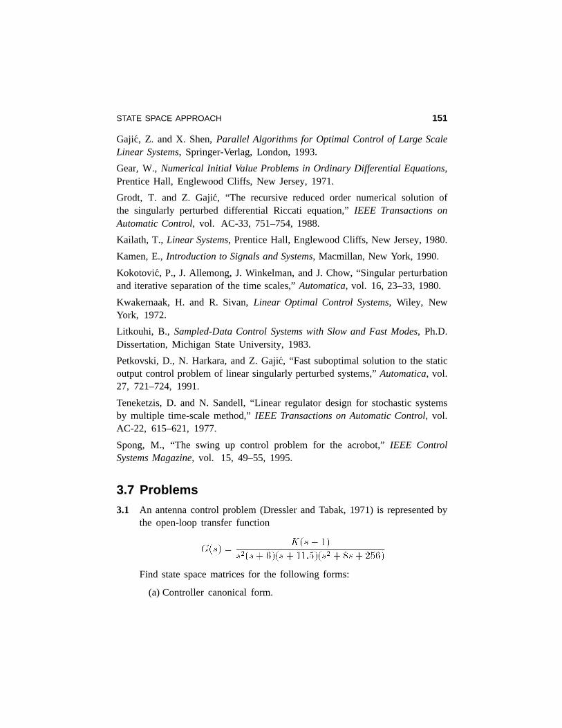
STATE SPACE APPROACH 151
Gajic, Z. and X. Shen,Parallel Algorithms for Optimal Control of Large ScaleLinear Systems, Springer-Verlag, London, 1993.
Gear, W.,Numerical Initial Value Problems in Ordinary Differential Equations,Prentice Hall, Englewood Cliffs, New Jersey, 1971.
Grodt, T. and Z. Gajic, “The recursive reduced order numerical solution ofthe singularly perturbed differential Riccati equation,”IEEE Transactions onAutomatic Control, vol. AC-33, 751–754, 1988.
Kailath, T.,Linear Systems, Prentice Hall, Englewood Cliffs, New Jersey, 1980.
Kamen, E.,Introduction to Signals and Systems, Macmillan, New York, 1990.
Kokotovic, P., J. Allemong, J. Winkelman, and J. Chow, “Singular perturbationanditerative separation of the time scales,”Automatica, vol. 16, 23–33, 1980.
Kwakernaak, H. and R. Sivan,Linear Optimal Control Systems, Wiley, NewYork, 1972.
Litkouhi, B., Sampled-Data Control Systems with Slow and Fast Modes, Ph.D.Dissertation, Michigan State University, 1983.
Petkovski, D., N. Harkara, and Z. Gajic, “Fast suboptimal solution to the staticoutput control problem of linear singularly perturbed systems,”Automatica, vol.27, 721–724, 1991.
Teneketzis, D. and N. Sandell, “Linear regulator design for stochastic systemsby multiple time-scale method,”IEEE Transactions on Automatic Control, vol.AC-22, 615–621, 1977.
Spong, M., “The swing up control problem for the acrobot,”IEEE ControlSystems Magazine, vol. 15, 49–55, 1995.
3.7 Problems3.1 An antenna control problem (Dressler and Tabak, 1971) is represented by
the open-loop transfer function
G(s) =K(s+ 1)
s2(s+ 6)(s+ 11:5)(s2 +8s+256)
Find state space matrices for the following forms:
(a) Controller canonical form.
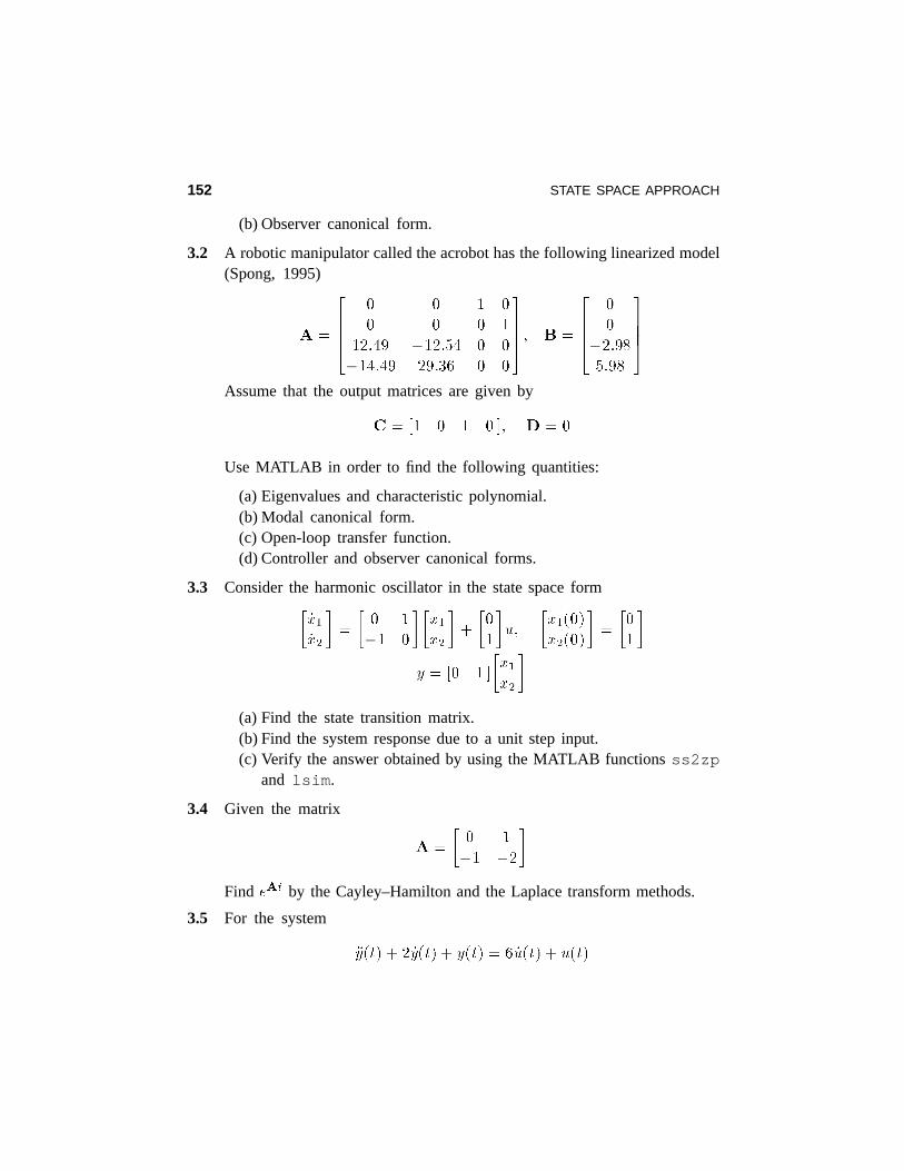
152 STATE SPACE APPROACH
(b) Observer canonical form.
3.2 A robotic manipulator called the acrobot has the following linearized model(Spong, 1995)
A =
26640 0 1 0
0 0 0 1
12:49 �12:54 0 0
�14:49 29:36 0 0
3775; B =
26640
0
�2:985:98
3775Assume that the output matrices are given by
C = [1 0 1 0 ]; D = 0
Use MATLAB in order to find the following quantities:
(a) Eigenvalues and characteristic polynomial.(b) Modal canonical form.(c) Open-loop transfer function.(d) Controller and observer canonical forms.
3.3 Consider the harmonic oscillator in the state space form�_x1_x2
�=
�0 1
�1 0
��x1x2
�+
�0
1
�u;
�x1(0)
x2(0)
�=
�0
1
�y = [0 1 ]
�x1x2
�(a) Find the state transition matrix.(b) Find the system response due to a unit step input.(c) Verify the answer obtained by using the MATLAB functionsss2zp
and lsim.
3.4 Given the matrix
A =
�0 1
�1 �2�
Find eAt by the Cayley–Hamilton and the Laplace transform methods.
3.5 For the system
�y(t) + 2 _y(t) + y(t) = 6 _u(t) + u(t)
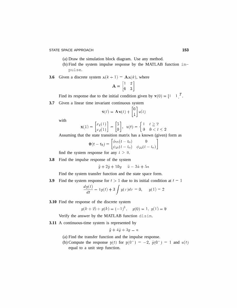
STATE SPACE APPROACH 153
(a) Draw the simulation block diagram. Use any method.(b) Find the system impulse response by the MATLAB functionim-
pulse.
3.6 Given a discrete systemx(k +1) = Ax(k), where
A =
�1 2
0 3
�Find its response due to the initial condition given byx(0) = [1 1 ]T .
3.7 Given a linear time invariant continuous system
_x(t) =Ax(t) +
�0
1
�u(t)
with
x(1) =
�x1(1)
x2(1)
�=
�5
0
�; u(t) =
�1 t � 2
0 0 < t � 2
Assuming that the state transition matrix has a known (given) form as
�(t� t0) =
��11(t� t0) 0
�21(t� t0) �22(t� t0)
�find the system response for anyt � 0.
3.8 Find the impulse response of the system
�y +2 _y + 10y = �u� 3 _u+5u
Find the system transfer function and the state space form.
3.9 Find the system response fort > 1 due to its initial condition att = 1
dy(t)
dt+ 4y(t) + 3
Zy(�)d� = 0; y(1) = 2
3.10 Find the response of the discrete system
y(k+ 2) + y(k) = (�1)k ; y(0) = 1; y(1) = 0
Verify the answer by the MATLAB functiondlsim.
3.11 A continuous-time system is represented by
�y + 4 _y +3y = u
(a) Find the transfer function and the impulse response.(b) Compute the responsey(t) for y(0�) = �2, _y(0�) = 1 and u(t)
equal to a unit step function.
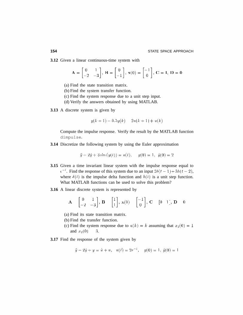
154 STATE SPACE APPROACH
3.12 Given a linear continuous-time system with
A =
�0 1
�2 �3�; B =
�0
�1
�; x(0) =
��1
0
�; C = I; D = 0
(a) Find the state transition matrix.(b) Find the system transfer function.(c) Find the system response due to a unit step input.(d) Verify the answers obtained by using MATLAB.
3.13 A discrete system is given by
y(k + 1)� 0:5y(k) = 2u(k + 1)+ u(k)
Compute the impulse response. Verify the result by the MATLAB functiondimpulse.
3.14 Discretize the following system by using the Euler approximation
�y + 2 _y + 3sin (y(t)) = u(t); y(0) = 1; _y(0) = 2
3.15 Given a time invariant linear system with the impulse response equal toe�t. Find the response of this system due to an input2�(t� 1)+3h(t� 2),where�(t) is the impulse delta function andh(t) is a unit step function.What MATLAB functions can be used to solve this problem?
3.16 A linear discrete system is represented by
A =
�0 1
�2 �3
�; B =
�1
1
�; x(0) =
��1
0
�; C = [0 1 ]; D = 0
(a) Find its state transition matrix.(b) Find the transfer function.(c) Find the system response due tou(k) = k assuming thatx1(0) = 1
and x2(0) = 3.
3.17 Find the response of the system given by
�y + 2 _y + y = _u + u; u(t) = 2e�t; y(0) = 1; _y(0) = 1
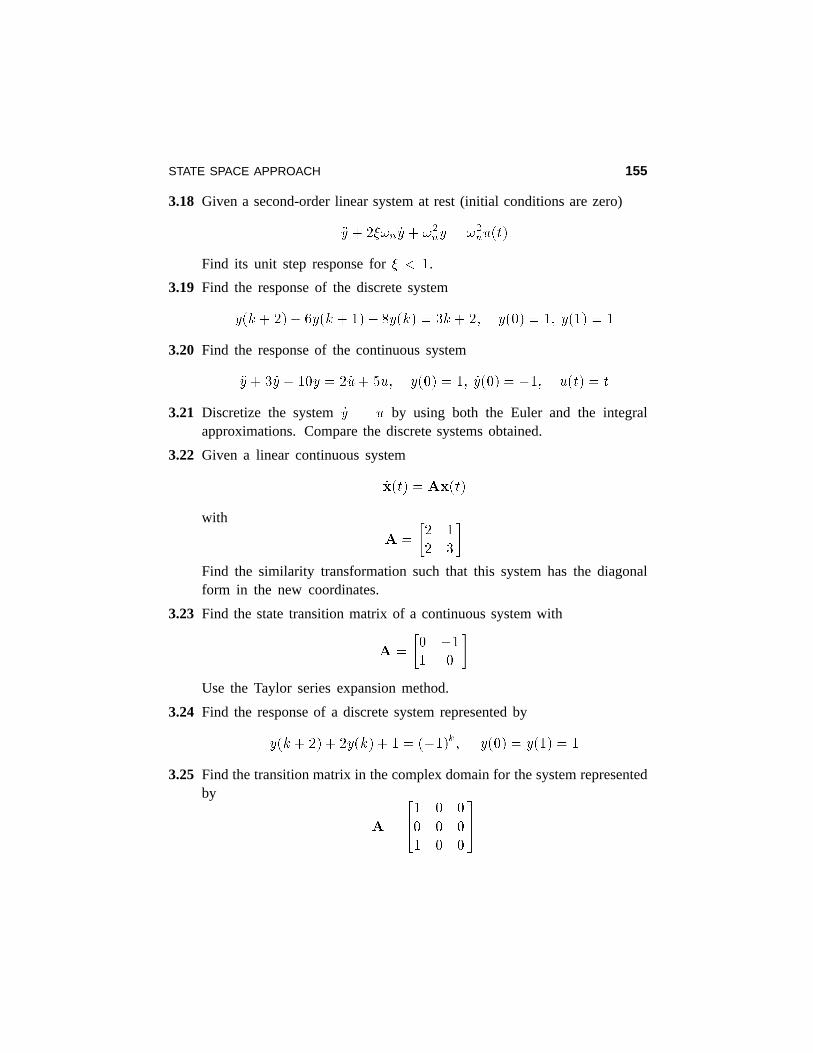
STATE SPACE APPROACH 155
3.18 Given a second-order linear system at rest (initial conditions are zero)
�y + 2�!n _y + !2ny = !2
nu(t)
Find its unit step response for� < 1.
3.19 Find the response of the discrete system
y(k + 2)� 6y(k+ 1) + 8y(k) = 3k+ 2; y(0) = 1; y(1) = 1
3.20 Find the response of the continuous system
�y + 3 _y � 10y = 2 _u+ 5u; y(0) = 1; _y(0) = �1; u(t) = t
3.21 Discretize the system_y = u by using both the Euler and the integralapproximations. Compare the discrete systems obtained.
3.22 Given a linear continuous system
_x(t) =Ax(t)
with
A =
�2 1
2 3
�Find the similarity transformation such that this system has the diagonalform in the new coordinates.
3.23 Find the state transition matrix of a continuous system with
A =
�0 �11 0
�Use the Taylor series expansion method.
3.24 Find the response of a discrete system represented by
y(k+ 2) + 2y(k) + 1 = (�1)k ; y(0) = y(1) = 1
3.25 Find the transition matrix in the complex domain for the system representedby
A =
241 0 0
0 0 0
1 0 0
35
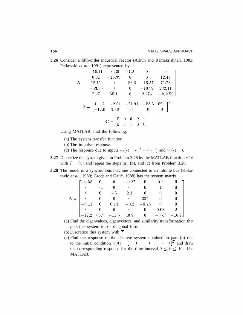
156 STATE SPACE APPROACH
3.26 Consider a fifth-order industrial reactor (Arkun and Ramakrishnan, 1983;Petkovskiet al., 1991) represented by
A =
266664�16:11 �0:39 27:2 0 0
0:01 �16:99 0 0 12:47
15:11 0 �53:6 �16:57 71:78
�53:36 0 0 �107:2 232:11
2:27 60:1 0 2:273 �102:99
377775B =
�11:12 �2:61 �21:91 �53:5 69:1
�12:6 3:36 0 0 0
�TC =
�0 0 0 0 1
0 1 1 0 0
�Using MATLAB, find the following:
(a) The system transfer function.(b) The impulse response.(c) The response due to inputsu1(t) = e�t + sin (t) andu2(t) = 0.
3.27 Discretize the system given in Problem 3.26 by the MATLAB functionc2dwith T = 0:1 and repeat the steps (a), (b), and (c) from Problem 3.26.
3.28 The model of a synchronous machine connected to an infinite bus (Koko-tovic et al., 1980; Grodt and Gajic, 1988) has the system matrix
A =
2666666664
�0:58 0 0 �0:27 0 0:2 0
0 �1 0 0 0 1 0
0 0 �5 2:1 0 0 0
0 0 0 0 337 0 0
�0:14 0 0:14 �0:2 �0:28 0 0
0 0 0 0 0 0:08 2
�17:2 66:7 �11:6 40:9 0 �66:7 �16:7
3777777775(a) Find the eigenvalues, eigenvectors, and similarity transformation that
puts this system into a diagonal form.(b) Discretize this system withT = 1.(c) Find the response of the discrete system obtained in part (b) due
to the initial conditionx(0) = [1 1 1 1 1 1 1 ]T and drawthe corresponding response for the time interval0 � k � 10. UseMATLAB.
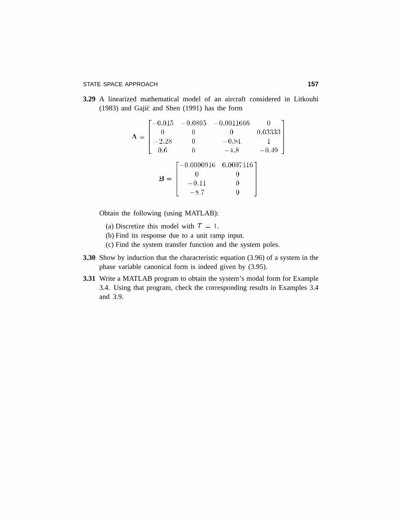
STATE SPACE APPROACH 157
3.29 A linearized mathematical model of an aircraft considered in Litkouhi(1983) and Gajic and Shen (1991) has the form
A =
2664�0:015 �0:0805 �0:0011666 0
0 0 0 0:03333
�2:28 0 �0:84 1
0:6 0 �4:8 �0:49
3775
B =
2664�0:0000916 0:0007416
0 0
�0:11 0
�8:7 0
3775Obtain the following (using MATLAB):
(a) Discretize this model withT = 1.(b) Find its response due to a unit ramp input.(c) Find the system transfer function and the system poles.
3.30 Show by induction that the characteristic equation (3.96) of a system in thephase variable canonical form is indeed given by (3.95).
3.31 Write a MATLAB program to obtain the system’s modal form for Example3.4. Using that program, check the corresponding results in Examples 3.4and 3.9.