A Buse , N Tischler , M L Juan and G Molina-Terriza zz cn p: L 2np

Where are photons created in parametric down

conversion? On the control of the spatio-temporal

properties of biphoton states

A Buse1, 2, 3, N Tischler1, 2, 3, M L Juan1, 2 and G

Molina-Terriza1, 2‡1 Centre for Engineered Quantum Systems, Macquarie University, NSW 2109,

Australia

2 Department of Physics & Astronomy, Macquarie University, NSW 2109, Australia

3 Joint first authors

E-mail: [email protected]

Abstract. In spontaneous parametric down-conversion photons are known to be

created coherently and with equal probability over the entire length of the crystal.

Then, there is no particular position in the crystal where a photon pair is created. We

make the seemingly contradictory observation that we can control the time delay with

the crystal position along the propagation direction. We resolve this contradiction by

showing that the spatio-temporal correlations critically affect the temporal properties

of the pair of photons, when using a finite detector size. We expect this to have

important implications for experiments that require indistinguishable photons.

‡ Corresponding author

arX

iv:1

502.

0277

3v1

[qu

ant-

ph]

10

Feb

2015

On the control of the spatio-temporal properties of biphoton states 2

1. Introduction

The nonlinear process of spontaneous parametric down-conversion (SPDC), in which

a small fraction of photons from an intense pump beam is converted into pairs of

lower energy photons, is currently the predominant method for producing photon pairs

[1, 2] and heralded single photons [3]. These are required for several applications

of quantum optics, including quantum computation [4], quantum metrology [5, 6],

quantum communication [7, 8], and fundamental tests of quantum mechanics [9, 10].

Such diversity of applications has been made available through the possibility to

tailor properties of the down-converted photons, which depend on the polarisation,

spectral/temporal, and spatial degrees of freedom. Photon pairs can be entangled

in each of, and even between, these degrees of freedom [11–15]. A lot of progress

has been made in developing ways to achieve frequency or momentum correlated,

uncorrelated, and anticorrelated states [16–21]. Temporal indistinguishability is a

common requirement for quantum optics experiments, especially in applications that

rely on quantum interference. In the case of type II SPDC sources this is often achieved

by birefringent compensation [10, 11, 22].

The photons from SPDC are generally well understood and known to be created

coherently and, in the absence of pump losses, with equal probability over the length

of the crystal [22]. In theory, the number of down-converted photons depends on the

total pump power and, unlike second harmonic generation, is independent of the pump

intensity distribution for a fixed pump divergence and power. This is basically due to the

low efficiency of the nonlinear effect which leaves the pump beam essentially undepleted.

The total number of photon pairs created is then independent of the location of the pump

beam relative to the crystal [23, 24]. On the other hand, under realistic experimental

conditions, the number of detected photons will strongly depend on the collection optics

and detector size.

Here we report the measurement of a time delay between the photon pair in type

II SPDC that depends on the position of the crystal. We will experimentally and

theoretically show that this effect is not due to a crystal localized photon creation

or detection. Instead, the cause of the tunable time delay can be attributed to the

particular spatio-temporal structure of the biphoton wavefunction. The frequency

momentum correlations induced by the SPDC process are akin to those present in

localized waves [25]. We show that the collection lens introduces a spatially dependent

quadratic phase, which through the spatio-temporal correlations, becomes a temporal

delay between the photon pairs arriving at the detectors.

When concentrating on either spectral or spatial correlations between signal and

idler photons, spatio-temporal correlations are often considered a nuisance and are

avoided through strong filtering in the other degree of freedom. However, without such

filtering, pronounced correlations exist between frequency and transverse momentum

[26]. These correlations are currently subject of intense research [27–30].

As explained in more detail in section 3, a popular SPDC source consists of a focused


pump beam, a nonlinear crystal designed for type II collinear down-conversion, and a

lens to collect the photon pairs. The usual protocol for setting the relative positions of

the crystal and collection lens is to centre the pump focal point in the middle of the

crystal and then set the collection lens to maximise the count rates. Hence, the positions

of the crystal and collection lens are fixed. One of the few investigations into the effect

the crystal position has on the two-photon state was done by Di Lorenzo Pires et al.,

who studied the near-field intensity patterns in type I emission [23]. In the following,

we also allow the crystal and collection lens positions to be variable and find that their

distance has a strong impact on the delay between signal and idler. We establish this

for single-mode fibre and free-space detection through both measurements and theory.

2. Theoretical Model

We will start by providing a complete theoretical model of the frequency and momentum

correlations of the biphoton wavefunction and their effect in relevant experimental

conditions. We therefore set out to calculate the number of coincidence counts as a

function of time delay between signal and idler photons from type II down-conversion,

arriving at the detector for two different detection schemes: single-mode fiber collection

and free space detection. Since we regard the pump focal position and distance between

crystal and collection lens as free parameters, they are to appear explicitly in the

calculation.

Let us begin with the biphoton wavefunction at the crystal exit facet, which already

contains the dependence on the pump focal position. Throughout this work, we will

model our experiment with a monochromatic pump beam, which means that signal and

idler frequencies add up to a fixed pump frequency. The biphoton wavefunction is

|Ψ〉 =∫

dqsdqidωs Φ(qs,qi, ωs, ωi)a†(qs, ωs, σs)a

†(qi, ωi, σi)|0〉, (1)

where s and i label signal and idler photons, q is the transverse wavevector, ω the

angular frequency, and σ the polarisation. a†(q, ω, σ) is the photon creation operator for

a photon mode characterized by transverse wavenumber, frequency, and polarisation.

Throughout this work, our integrals are implied to be over all possible values of the

integration variables, unless specified otherwise. Φ(qs,qi, ωs, ωi) is the biphoton mode

function, which takes on the form

Φ(qs,qi, ωs, ωi) ∝ sinc

(∆kz(qs,qi, ωs, ωi)L

2

)exp

(−w

2|qs + qi|24

)× exp(i kpz(zc − zfoc(zc)))× exp(i (ksz(ωs,qs) + kiz(ωi,qi)) L/2). (2)

Here L is the crystal length, w the pump beam waist, ∆kz the longitudinal wave vector

mismatch kpz − ksz − kiz − 2πΛ

and Λ the poling period of the crystal. ωi is not an

independent variable as it is given by ωi = ωp−ωs, but we do keep it in the expressions

for the sake of clarity. Our main experiment consists in longitudinally displacing the


Figure 1. (a) Longitudinal shift of the pump focus caused by a translation of the

crystal. z = 0 is the reference position at which the pump focus coincides with the

crystal centre. zc is the position of the crystal centre and zfoc the position of the

pump focus. L is the length of the crystal. This configuration is similar to the one

used in [23]. (b) Illustration of our geometry after the crystal. zCL is the position of

the collection lens which has a focal length f1. d is the distance between a point one

focal distance before the collection lens, and the crystal end.

crystal, and to model this process, we need to consider the effect this has on the pump

focal position. The geometry is illustrated in figure 1. zc denotes the position of the

crystal centre and zfoc(zc) the focus of the pump beam, both relative to the position at

which the focus coincides with the crystal centre (i.e. zfoc = 0 when zc = 0). Clearly, in

the commonly assumed case of the pump focal point lying at the centre of the crystal,

the exp(i kpz(zc − zfoc(zc))) term disappears. Assuming the pump beam is paraxial, its

focal position in the laboratory frame is given by:

zfoc(zc) =

L2− L

2np: zc ≤ − L

2np

zc − npzc : − L2np

< zc <L

2np

−L2

+ L2np

: zc ≥ L2np,

(3)

where np is the refractive index of the crystal experienced by the pump beam. The

crystal positions |zc| = L2np

correspond to the pump focus lying at one of the crystal

facets. Within the crystal, the pump focal position shifts in the opposite direction to

the crystal movement. Once shifted out of the crystal in either direction, it no longer

depends on the crystal position. As mentioned earlier, from here there are two possible

treatments of the spatial degree of freedom, depending on the detection scheme used.

For single-mode fibre detection, a projection into a Gaussian detection mode is

performed. We can do this at the crystal end facet where we have the expression for

the biphoton wavefunction (1,2). The Gaussian detection mode is

Gspa(q)z=zc+L/2 =wf√2π

exp

(−w

2f |q|24

)exp

(−i |q|

2d

2kair(ω)

), (4)

where wf is the detection mode beam waist, and kair(ω) = ωc

is the wavenumber of the

detected photon in air, c being the speed of light in vacuum. The Gaussian mode is

effectively characterised by two things, the distance of the crystal end from where the


detection focal point would be in the absence of the crystal, d =(f1 − (zCL − zc − L

2)),

and the beam waist, wf . The optimal detection beam waist depends on the pump

beam waist among other things, and a body of work on this subject is available in the

literature [31–33]. Usually, the detection focal point is assumed to lie at the centre of

the crystal, coinciding with the pump focal point, and this imposes a particular distance

from the crystal end to where the detection focal point would be without the crystal,(L/2n

). The position of the collection lens for this case is zCL = L

2− L/2

n+ f1. As we

allow for longitudinal translations of the collecting lens, zCL will remain a parameter in

our calculations. After projection of the photons into Gaussian detection modes with

equal detection beam waists for signal and idler, the wavefunction reads:

|ΨSMF 〉 =∫

dωs ΦSMF (ωs, ωi)a†(ωs, σs)a

†(ωi, σi)|0〉,

ΦSMF (ωs, ωi) =∫

dqsdqiΦ(qs,qi, ωs, ωi)G∗spa(qs)G

∗spa(qi). (5)

In order to calculate the time delay distribution between the arrival times of signal and

idler photons, the following expression is evaluated:

Rcoinc,SMF (τ) ∝ |〈0|E(+)i (t− τ/2)E(+)

s (t+ τ/2)|ΨSMF 〉|2, (6)

where the operator E(+)j (t) is proportional to

∫dω exp(−iωt)a(ω, σj). The reason t does

not appear on the left-hand-side is that for a monochromatic pump beam, the quantity

is independent of the mean time; it only depends on the time difference.

In contrast to the single-mode fibre case where only one spatial mode is relevant at

the detector, for free-space detection, the counts as a function of time delay need to be

calculated for all pairs of points on the detector surfaces, and subsequently integrated

over all such available pairs:

Rcoinc,FS(τ) =∫

Adet

drsdriRcoinc,PP (rs, ri, τ)

∝∫

Adet

drsdri|〈0|E(+)i (ri, t− τ/2)E(+)

s (rs, t+ τ/2)|Ψ〉|2 (7)

The electric field operator at the detector plane can be related to the annihilation

operator at the crystal exit facet using a thin lens model from Fourier optics and the

Fresnel approximation:

E(r, t)z=zdet =∫

dω dq exp

(−if1

f2

r · q− iωt)

× exp (−ikair,zd) a(q, ω)z=zc+L/2

≈∫

dω dq exp

(−if1

f2

r · q− iωt)

× exp

(i

(−kair(ω) +

|q|22kair(ω)

)d

)a(q, ω)z=zc+L/2, (8)

where f1 and f2 are the focal lengths of the collection lens and of the focusing lenses

in front of the detectors, respectively. For each pair of points that contribute to the

integral in equation (7) and for the expression from the Gaussian detection scheme (6),


0 2 4 6 8

−2

0

2

·105

|Ω| (THz)

q x(m

−1)

(a)

0

max

0.0 2.0 4.0 6.00.0

0.5

1.0

Time delay(ps)

Coi

ncid

ence

s(a

rb.u

nits

) (b)

Figure 2. (a) Calculated spatio-temporal correlations of the SPDC wavefunction

for experimentally relevant parameters. What we depict is proportional to the

probabilities of different qx, Ω values for a photon with qy = 0, after having traced

out the other photon of the pair. The overlaid line illustrates the linear dependence

between Ω and |q|2. (b) Simulated time delay distribution between signal and idler

photons for single-mode fibre detection, with the crystal in the central position (solid

line) and shifted by 1 mm (dashed line).

the coincidence counts as a function of time delay can be cast in the form of

Rcoinc(τ) ∝∣∣∣∣ ∫ dqsdqidΩ exp (i(ksz(−Ω,qs) + kiz(Ω,qi)) L/2)

× exp

(id

(|qs|2

2kair(−Ω)+|qi|2

2kair(Ω)

))

× sinc(

∆kzL

2

)g(qs,qi, zc) exp(iΩτ)

∣∣∣∣2. (9)

Ω is defined as Ω = ωi − ωp/2, and the shorthand of kair(Ω) means kair(ω) =

kair(ωp/2 + Ω). g(qs,qi, zc) incorporates the remaining terms and depends on the

type of detection and on the crystal position through the pump focal position.

The term that models a change in the distance between crystal and collection lens

is exp(id(

|qs|22kair(−Ω)

+ |qi|22kair(Ω)

)). What impact does such a transverse momentum-

dependent phase have on the time delay? A potential impact must be mediated

by spatio-temporal correlations. Hence, a way to develop an understanding is by

considering the form of spatio-temporal correlations imposed by the phase-matching

conditions of SPDC.

To gain an intuitive picture of the system, in the following we develop a toy model

by introducing approximations. We will, however, come back to the exact equations

(6) and (7) for the simulation which we compare to the experimental results in section

4. To learn about the spatio-temporal correlations, we perform a multivariate Taylor

approximation of ksz, kiz and ∆kz, about the collinear degenerate case up to the first

nonzero terms. The reference, for which we take kpz − ksz − kiz − 2πΛ

= 0, is therefore at

Ω = 0, T = T0, qs = qi = 0 (T is the crystal temperature). For now, we will further

simplify our analysis by considering the case of a plane wave pump beam with qp = 0


for our toy model. This imposes −qs = qi ≡ q, and hence |qs|2 = |qi|2 = |q|2 which

will allow us to immediately draw some interesting conclusions:

∆kz ≈ ΩD + (T − T0)E +|q|2

2ks(0)+|q|2

2ki(0), (10)

where D =(∂ks∂Ω− ∂ki

∂Ω

)and E =

(∂kp∂T− ∂ks

∂T− ∂ki

∂T

). From now on, all derivatives are

evaluated at the reference settings mentioned above. With very long crystals and plane

wave pump beam, the photons would be generated only in the perfect phase matching

condition, ∆kz = 0. We see that this case entails a linear dependence between Ω

and |q|2, indicated by the overlaid line in figure 2 (a) and also shown in reference

[28]. As a result, the q-dependent phase term induced by the coupling lens causes a

shift of the time delays which is proportional to the change in distance between the

crystal and the coupling lens. This is the main mechanism we have identified causing

the observed crystal dependent time delay of the emitted photons. We would like to

note that the absence of the linear term in momentum in Eq. (10) is due to the fact

that in our configuration the photons propagate along one of the optical axes; in other

configurations there can be a linear dependence in the momentum [34].

Let’s go back to the finite crystal model where the sinc function actually results in a

spread of |q|2 values for a given Ω value. To account for this spread and deepen our first

grasp of the underlying physics, let us analyse (9), again using the Taylor approximation

of the longitudinal wavevector mismatch (10).

Rcoinc(τ) ∝∼∣∣∣∣ ∫ dqdΩ exp

(iL

2

(ks(0) + ki(0) + (T − T0)

(∂ks∂T

+∂ki∂T

)− ΩD

))

× exp

(id

(|q|2

2kair(−Ω)+

|q|22kair(Ω)

))

× sinc

((ΩD + (T − T0)E +

|q|22ks(0)

+|q|2

2ki(0)

)L

2

)g(q) exp(iΩτ)

∣∣∣∣2 (11)

Since we are assuming a plane wave pump and therefore qs = −qi, the integrals over

signal and idler transverse momenta were replaced by an integral over one transverse

momentum. Importantly, note that the dependence of g on the crystal position, zc, has

also dropped out for a plane wave pump. We can now proceed with equation (11) as

follows: Since we are taking the modulus, we can remove the phase that is independent

of the integration variables. We next evaluate the integral over Ω, which is an inverse

Fourier transform of a sinc function. Then, the functions that contain no dependence

on q can be taken outside of the remaining integral. This leaves us with

Rcoinc(τ) ∝∼∣∣∣∣ 2π

DLrect

(1

DL

(τ −DL

2

))×∫

dq exp

(id

(|q|2

2kair(−Ω)+

|q|22kair(Ω)

))

× exp

(−i(τ −DL

2

)1

D

(|q|2

2ks(0)+|q|2

2ki(0)

))g(q)

∣∣∣∣2 (12)


At this point, making the approximation of ks(0) ≈ ki(0) ≈ nkair(Ω) ≈ nkair(−Ω) ≈nkair(0) shows us the primary effect of changing the distance between crystal and

collection lens:

Rcoinc(τ) ∝∼2π

DLrect

(1

DL

(τ −DL

2

))×∣∣∣∣ ∫ dq exp

(−i|q|2

nDkair(0)(τ − τ0)

)g(q)

∣∣∣∣2 (13)

where τ0 = DL/2 + nD(f1 − zCL + zc +L/2). The two key outcomes we can learn from

the simplified expression (13) are the rectangular function and the shift in τ within

the integral. The rectangular function has a width of DL and is centred such that the

nonzero interval begins at 0. It physically corresponds to the time delays photons can

acquire throughout the length of the crystal and ensures that the time delay distribution

can only be nonzero in this specific interval. As for the specific shape of the time

delay distribution, this depends on g(q), which means that it is not predicted with

this general analysis. The important thing, however, is that within the applicability of

the approximations made, a change in the distance between collection lens and crystal,

zCL− zc, results in a shift of the time delay distributions, except for the fixed cut-off by

the rectangular function. The shift is given by nD∆z, where ∆z is the displacement of

the crystal or collection lens. It is important to bear in mind that this analysis applies

to the case of fibre-coupled detection and to individual pairs of points on the detectors

contributing to the free-space detection.

We have evaluated the biphoton mode function and coincidences given by (6) and

(7) numerically without the approximations made later on, with the refractive indices

modeled by temperature-dependent Sellmeier equations. A temperature dependence of

the poling period caused by thermal expansion of the crystal was also taken into account

based on coefficients from [35], although this has a comparatively small impact. One of

the detection schemes incorporates a bandpass filter, which we model with a Gaussian

spectral transmission function applied to the biphoton wavefunction. The parameters

required as inputs to the simulations for modelling the experiments are i. the fixed

and known crystal length, poling period, and pump wavelength, ii. the variable but

known pump beam waist and crystal temperature, and iii. the variable detection beam

waist (for single-mode fibre detection) or detection area (for free-space detection). The

detection beam waist was not measured experimentally but adjusted to optimise counts,

and the free-space detection area is nominally (50 µm)2 but needed to be adjusted in

the simulations to account for an imperfect imaging system.

To demonstrate the applicability of our analytic results from the toy model, which

assumes a plane wave pump and is based on a Taylor approximation of the wavevector

mismatch, to our experimental case of a focused pump beam, we present simulation

results in figure 2 without the use of those approximations. Figure 2 (a) shows the

spatio-temporal correlations for our set-up, with the linear dependence between |q|2 and

Ω illustrated. It is interesting to note that this dependence differs from the case of type I

down-conversion [27, 29, 30] due to the nonzero difference in the group velocities of signal


and idler. The main outcomes from the simplified expression (13) can be recognised in

figure 2 (b), which shows time delay distributions for two different crystal positions

using the single-mode fibre detection scheme. As discussed, the time delay distribution

is shifted when the crystal is displaced, except for a fixed cut-off that remains and is

modelled by the rectangular function. Of course unlike for a plane wave pump, the

pump focal position comes into play for a focused pump. In our work we found that

the focal position of the pump beam has little effect on the time delay shift, but has

a significant impact on the proportion of photons detected, particularly depending on

whether the pump and detection focal positions match up.

3. Experimental Method

Figure 3. Schematic of the experimental set-up. The 404.25 nm pump laser is

expanded with a telescope to obtain a specific beam waist in the nonlinear crystal. A

half waveplate (HWP) controls the polarisation relative to the crystallographic axes.

A lens then focuses the collimated beam into the periodically poled potassium titanyl

phosphate (ppKTP) crystal, from where the down-converted photons are collected by a

collection lens. The pump beam is blocked by a longpass or interference bandpass filter.

Signal and idler are separated by a polarising beam splitter (PBS) and subsequently

either directly detected by two free-space avalanche photo diodes (APD) or first coupled

to single-mode fibres and then detected. The time difference between signal and idler

is measured with a time correlated single photon counting system.

After describing theoretically the spatio-temporal correlations of the down-

converted photons and their effect on the time delays in the detection of the photons,

let us turn to describe our experimental apparatus and results. In figure 3 we show the

experimental set-up used to create the SPDC photon pairs and how the time delay is

measured. A continuous wave (CW), single frequency, diode laser with a wavelength of


13.45 13.50 13.55 13.60 13.650

20,000

40,000

60,000

Arrival time difference (ns)

Num

ber

ofph

oton

s

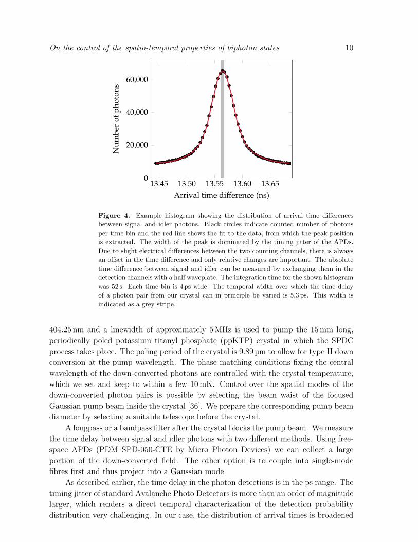
Figure 4. Example histogram showing the distribution of arrival time differences

between signal and idler photons. Black circles indicate counted number of photons

per time bin and the red line shows the fit to the data, from which the peak position

is extracted. The width of the peak is dominated by the timing jitter of the APDs.

Due to slight electrical differences between the two counting channels, there is always

an offset in the time difference and only relative changes are important. The absolute

time difference between signal and idler can be measured by exchanging them in the

detection channels with a half waveplate. The integration time for the shown histogram

was 52 s. Each time bin is 4 ps wide. The temporal width over which the time delay

of a photon pair from our crystal can in principle be varied is 5.3 ps. This width is

indicated as a grey stripe.

404.25 nm and a linewidth of approximately 5 MHz is used to pump the 15 mm long,

periodically poled potassium titanyl phosphate (ppKTP) crystal in which the SPDC

process takes place. The poling period of the crystal is 9.89 µm to allow for type II down

conversion at the pump wavelength. The phase matching conditions fixing the central

wavelength of the down-converted photons are controlled with the crystal temperature,

which we set and keep to within a few 10 mK. Control over the spatial modes of the

down-converted photon pairs is possible by selecting the beam waist of the focused

Gaussian pump beam inside the crystal [36]. We prepare the corresponding pump beam

diameter by selecting a suitable telescope before the crystal.

A longpass or a bandpass filter after the crystal blocks the pump beam. We measure

the time delay between signal and idler photons with two different methods. Using free-

space APDs (PDM SPD-050-CTE by Micro Photon Devices) we can collect a large

portion of the down-converted field. The other option is to couple into single-mode

fibres first and thus project into a Gaussian mode.

As described earlier, the time delay in the photon detections is in the ps range. The

timing jitter of standard Avalanche Photo Detectors is more than an order of magnitude

larger, which renders a direct temporal characterization of the detection probability

distribution very challenging. In our case, the distribution of arrival times is broadened


by the timing jitter of both APDs to a full width at half maximum of about 50 ps. On

the other hand, the average time delay is amenable to be measured by carefully fitting

the arrival time distribution. This measurement is only limited by the signal to noise in

the measurements and the stability of the single photon counting system (PicoHarp 300

from PicoQuant). A typical histogram is shown in figure 4, together with an empirical

fit that is used to extract the peak position and thus the average arrival time difference

between signal and idler. The fitting model which was validated by the experimental

data is based on a sum of two Gaussian profiles with different widths, positions and

amplitudes, plus a constant background. This model contains just 7 free parameters

from which we can extract the peak position. As the model fits very well the collected

data, the error in the peak position is much smaller than the bin size. To further reduce

the uncertainty, we acquire several histograms per crystal or collection lens position and

average over the resulting peak positions. As a result we are able to measure average

time differences much smaller than the time-binning of the histogram. To correct for

a slow drift of the electronics, we acquire additional histograms at a reference position

after each measurement. Both nonlinear crystal and the collection lens are mounted on

motorized stages to scan their position and record the corresponding time difference.

4. Experimental Results and Comparison with Theory

−5 0 50

2

4

Crystal z-position (mm)

Tim

ede

lay

(ps)

(a)

−10 −5 0 5 100

2

4


(b)

−10 −5 0 5 100

2

4


(c)

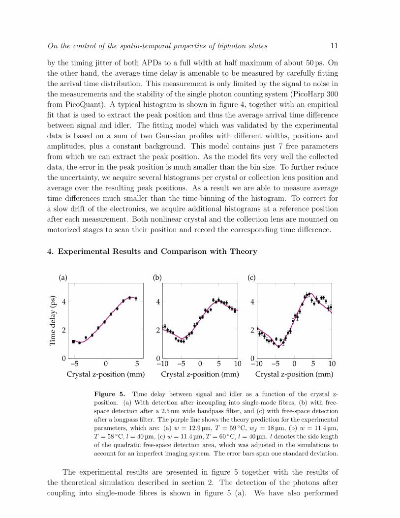
Figure 5. Time delay between signal and idler as a function of the crystal z-

position. (a) With detection after incoupling into single-mode fibres, (b) with free-

space detection after a 2.5 nm wide bandpass filter, and (c) with free-space detection

after a longpass filter. The purple line shows the theory prediction for the experimental

parameters, which are: (a) w = 12.9 µm, T = 59 C, wf = 18 µm, (b) w = 11.4 µm,

T = 58 C, l = 40 µm, (c) w = 11.4 µm, T = 60 C, l = 40 µm. l denotes the side length

of the quadratic free-space detection area, which was adjusted in the simulations to

account for an imperfect imaging system. The error bars span one standard deviation.

The experimental results are presented in figure 5 together with the results of

the theoretical simulation described in section 2. The detection of the photons after

coupling into single-mode fibres is shown in figure 5 (a). We have also performed


free-space detection with a spectral filter of width 2.5 nm (FWHM), figure 5 (b), and

without spectral filtering, figure 5 (c). The simulation is based on the experimental

parameters and the only adjustable parameter is the detection beam waist or detector

size, depending on the type of measurement.

The results from different detection schemes are qualitatively similar. Each set of

results shows a monotonic change in time delay within the range of crystal positions

for which the detection focal point lies within the crystal, an interval of approximately

8 mm. As mentioned above, in our convention the 0 crystal position is such that the

pump and detection focal points coincide with the centre of the crystal. The range

of time delays depicted in the figure corresponds to orthogonally polarised photons

propagating a distance of up to the full crystal length in the birefringent crystal medium.

Mathematically, these limits correspond to the cut-off by the rectangular function in

equation (13). A nonzero width in the distribution of time delays reduces the range

of observed values since we are working with average time delays. The turning points

visible in each case occur when the peak in the time delay distribution is shifted past the

cut-off. Since we are measuring an average rather than the position of the maximum,

shifting the peak past the cut-off results in the average moving back towards the central

value.

In addition to the dependencies shown, the specific shapes are further influenced by

the detection beam waist for single-mode fibre coupling, the detector size for free-space

measurement, and the crystal temperature. Spectral filtering is a common practice

for a number of purposes such as decreasing the distinguishability of the two photons,

and one of the other reasons is the frequently desired consequence of reducing spatio-

temporal correlations. However, as figure 5 shows, the difference between the cases with

and without spectral filtering is relatively minor, so in our case the reduction in the

correlations was not sufficient to eliminate the mechanism. As mentioned previously,

the distance between crystal and collection lens results in a particular time delay

distribution. It is therefore also possible to achieve a change in time delay by moving

the collection lens instead of the crystal. We have tried this in both experiment and

theory and obtained results similar to those shown in figure 5. However, changing the

crystal position is experimentally more relevant since this keeps the collimation of the

beam after the collection lens intact.

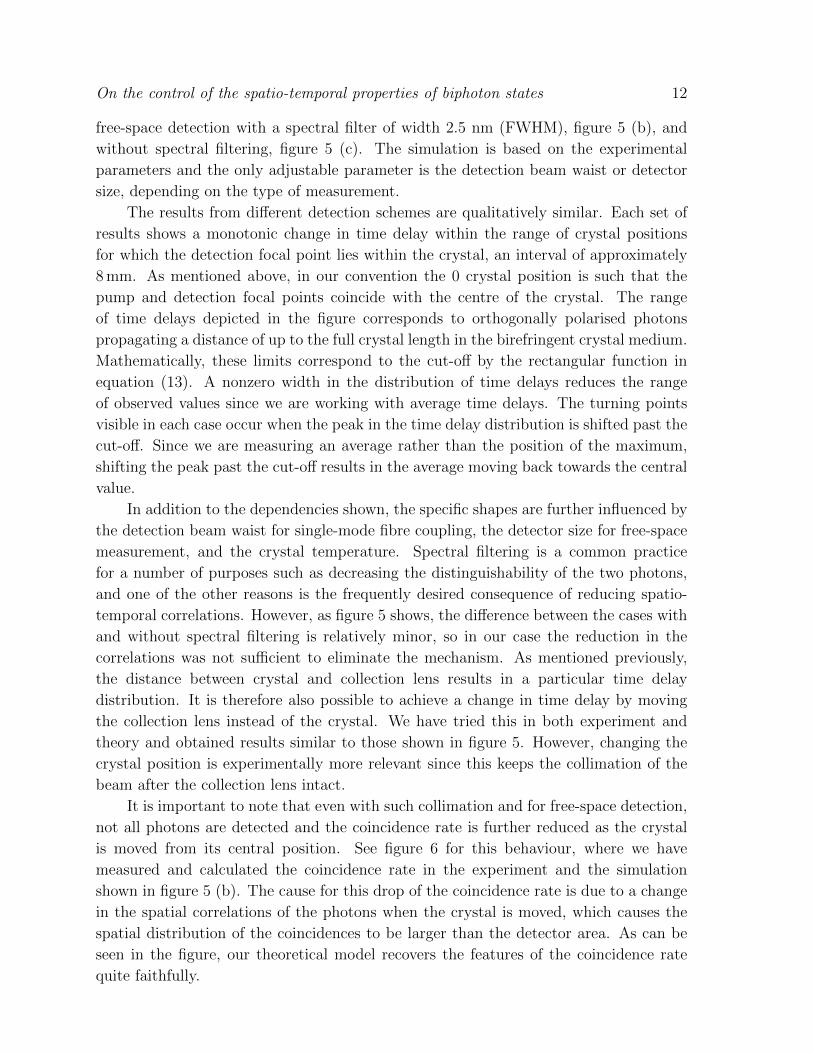
It is important to note that even with such collimation and for free-space detection,

not all photons are detected and the coincidence rate is further reduced as the crystal

is moved from its central position. See figure 6 for this behaviour, where we have

measured and calculated the coincidence rate in the experiment and the simulation

shown in figure 5 (b). The cause for this drop of the coincidence rate is due to a change

in the spatial correlations of the photons when the crystal is moved, which causes the

spatial distribution of the coincidences to be larger than the detector area. As can be

seen in the figure, our theoretical model recovers the features of the coincidence rate

quite faithfully.


−10 −5 0 5 100.0

0.5

1.0

Crystal position (mm)N

orm

alis

edco

inci

denc

era

te

Figure 6. The coincidence count rate drops as the pump and detection foci move away

from the centre of the crystal. Depicted are results for the free-space detection scheme

with the 2.5 nm wide bandpass filter. The purple line shows the theory prediction,

where the same parameters were used as for figure 5 (b).

5. Discussion

It is well known that SPDC is a coherent process and photons generated throughout the

whole length of the crystal contribute to the biphoton wavefunction equally [22]. With

this in mind, it is somewhat surprising to observe a change in time delay. The resolution

lies in the fact that we do not detect all photons generated in the crystal. This is obvious

for the case of single-mode fibre detection, where a significant portion of the down-

converted field is rejected. Using a free-space detection scheme considerably increases

the number of collected photons, but nonetheless, not all photons are collected due to

the finite detector size. Indeed, in the simulations we only recover the experimentally

measured change in time delay after restricting the collection of photons in space,

compared to an infinite detector area. We believe such a loss of photons may also have

caused the change of counts in [37], from which the authors then infer a dependence

of the SPDC efficiency on the pump beam intensity. Changing the distance between

crystal and collection lens is modeled by the phase term exp(id(

|qs|22kair(−Ω)

+ |qi|22kair(Ω)

))where d =

(f1 −

(zCL − zc − L

2

)). This term influences the time delay due to spatio-

temporal correlations.

The time delay between photons plays an important role in quantum interference

experiments such as the one by Hong, Ou, and Mandel [38]. In the case where the

photons travel along separate paths before incidence on the beam splitter, it is easy to

control the path length difference over a wide range. In contrast, a Hong-Ou-Mandel

experiment in which signal and idler photons travel along the same path before arriving

at a polarising beam splitter [39, 40], requires birefringent materials to control the time

delay. When using a fixed delay compensation, our results show that it is important

to have the crystal and collection lens positioned correctly, even if spectral filtering

comparable to our 2.5 nm bandpass filter is performed. This is particularly relevant

for the increasingly popular use of long crystals for bright sources of photon pairs,


made possible through the use of periodic poling. Conversely, our observed dependence

could also be harnessed by controlling the time delay through a deliberate positioning

of the crystal. It is important to keep in mind, however, that the change in time delay

achieved in this way is not equivalent to a shift in the complete time delay distribution,

as is the case with a relative difference in free-space propagation lengths, and that it is

influenced by the restricted detection. The restriction of the detection depends on the

ratio of the focal lengths of the collection lens and the lenses before the detectors, and

on the detector area.

It is interesting to compare our findings with reference [41]. Similarly to our work,

a quadratic phase associated with the displacement of an experimental component was

shown to be responsible for a change of the time delay distribution. However, since

the type I phase matching in that case entails different spatio-temporal correlations, a

dispersion like effect instead of a time delay shift was observed.

Throughout this work, we have presented results of average time delays.

Experimentally, this was necessary because of the timing jitter of the detectors, which

is much larger than the range of observed changes. In future experiments, it would be

interesting to extract more information about the time delay distribution.

6. Conclusion

We have shown for a number of experimentally relevant detection schemes, that the

average time delay between signal and idler photons in type II collinear down-conversion

depends on the distance between the nonlinear crystal and the collection lens. The

possible change of time delay covers a large portion of the total delay photon pairs can

acquire by propagating through the whole length of the crystal. We have measured

the time delay for single-mode fibre detection, as well as free-space detection with and

without spectral filtering. The experimental results are well described by our model.

The reason for the change in time delay are spatio-temporal correlations and the selective

nature of the detection, even in the case of free-space measurements. On the one

hand, the observed effect is something to beware of when indistinguishable photons

are required. On the other hand, when used deliberately, this constitutes a novel way

to tune the delay.

References

[1] Clausen C, Usmani I, Bussieres F, Sangouard N, Afzelius M, de Riedmatten H and Gisin N 2011

Nature 469 508–11

[2] Kim Y H, Kulik S and Shih Y 2001 Physical Review Letters 86 1370–1373

[3] Fasel S, Alibart O, Tanzilli S, Baldi P, Beveratos A, Gisin N and Zbinden H 2004 New Journal of

Physics 6 163–163

[4] Walther P, Resch K J, Rudolph T, Schenck E, Weinfurter H, Vedral V, Aspelmeyer M and Zeilinger

A 2005 Nature 434 169–76

[5] Sergienko A and Jaeger G 2003 Contemporary Physics 44 341–356

[6] Afek I, Ambar O and Silberberg Y 2010 Science 328 879–881


[7] Trifonov a and Zavriyev a 2005 Journal of Optics B: Quantum and Semiclassical Optics 7 S772–

S777

[8] Ursin R, Tiefenbacher F, Schmitt-Manderbach T, Weier H, Scheidl T, Lindenthal M, Blauensteiner

B, Jennewein T, Perdigues J, Trojek P, Omer B, Furst M, Meyenburg M, Rarity J, Sodnik Z,

Barbieri C, Weinfurter H and Zeilinger A 2007 Nature Physics 3 481–486

[9] Dada A C, Leach J, Buller G S, Padgett M J and Andersson E 2011 Nature Physics 7 677–680

[10] Tittel W and Weihs G 2001 Quantum Information and Computation 1 1–54

[11] Wong F N C, Shapiro J H and Kim T 2006 Laser Physics 16 1517–1524

[12] Kwiat P G, Steinberg A M and Chiao R Y 1993 Physical Review A 47 R2472–R2475

[13] Molina-Terriza G, Torres J P and Torner L 2007 Nature Physics 3 305–310

[14] Barreiro J T, Langford N K, Peters N A and Kwiat P G 2005 Physical Review Letters 95 1–4

[15] Nagali E and Sciarrino F 2010 Optics Express 18 18243–18248

[16] Grice W P, Bennink R S, Goodman D S and Ryan A T 2011 Physical Review A 83 023810

[17] Hendrych M, Micuda M and Torres J P 2007 Optics Letters 32 2339–2341

[18] Rangarajan R, Vicent L E, U’Ren A B and Kwiat P G 2011 Journal of Modern Optics 58 318–327

[19] Shimizu R and Edamatsu K 2009 Optics Express 17 16385–93

[20] Yun S, Xu P, Zhao J S, Gong Y X, Bai Y F, Shi J and Zhu S N 2012 Physical Review A 86 023852

[21] Valencia A, Cere A, Shi X, Molina-Terriza G and Torres J 2007 Physical Review Letters 99 243601

[22] Shih Y 2003 Reports on Progress in Physics 66 1009–1044

[23] Di Lorenzo Pires H, Coppens F M G J and van Exter M P 2011 Physical Review A 83 033837

[24] Bennink R, Liu Y, Earl D D and Grice W 2006 Physical Review A 74 023802

[25] Saari P and Reivelt K 2004 Physical Review E 69 036612

[26] Osorio C I, Valencia A and Torres J P 2008 New Journal of Physics 10 113012

[27] Gatti A, Brambilla E, Caspani L, Jedrkiewicz O and Lugiato L 2009 Physical Review Letters 102

223601

[28] Brambilla E, Caspani L, Lugiato L A and Gatti A 2010 Physical Review A 82 013835

[29] Gatti A, Corti T, Brambilla E and Horoshko D B 2012 Physical Review A 86 053803

[30] Gatti A, Caspani L, Corti T, Brambilla E and Jedrkiewicz O 2014 International Journal of

Quantum Information 12 1461016

[31] Bennink R S 2010 Physical Review A 81 053805

[32] Smirr J L, Deconinck M, Frey R, Agha I, Diamanti E and Zaquine I 2013 Journal of the Optical

Society of America B 30 288

[33] Guerreiro T, Martin A, Sanguinetti B, Bruno N, Zbinden H and Thew R T 2013 Optics Express

21 27641–27651

[34] Brida G, Chekhova M, Genovese M and Krivitsky L 2007 Phys. Rev. A 76(5) 053807

[35] Pignatiello F, De Rosa M, Ferraro P, Grilli S, De Natale P, Arie A and De Nicola S 2007 Optics

Communications 277 14–18

[36] Law C and Eberly J 2004 Physical Review Letters 92 127903

[37] Suzer O and Goodson T G 2008 Optics Express 16 20166–75

[38] Hong C K, Ou Z Y and Mandel L 1987 Physical Review Letters 59 2044–2046

[39] Resch K, Lundeen J and Steinberg A 2001 Physical Review A 63 020102

[40] Kuklewicz C, Fiorentino M, Messin G, Wong F and Shapiro J 2004 Physical Review A 69 013807

[41] Jedrkiewicz O, Blanchet J L, Brambilla E, Di Trapani P and Gatti A 2012 Physical Review Letters

108 253904

Documents

A Buse , N Tischler , M L Juan and G Molina-Terriza zz cn p: L 2np