© 2017 IEEE. Personal use of this material is permitted. Permission from IEEE must be obtained for

all other uses, in any current or future media, including reprinting/republishing this material for

advertising or promotional purposes, creating new collective works, for resale or redistribution to

servers or lists, or reuse of any copyrighted component of this work in other works.

Distance Function based 6DOF Localization for Unmanned AerialVehicles in GPS Denied Environments

James Unicomb1, Lakshitha Dantanarayana∗1, Janindu Arukgoda1,Ravindra Ranasinghe1, Gamini Dissanayake1, and Tomonari Furukawa2

Abstract— This paper presents an algorithm for localizing anunmanned aerial vehicle (UAV) in GPS denied environments.Localization is performed with respect to a pre-built map of theenvironment represented using the distance function of a binarymosaic, avoiding the need for extraction and explicit matchingof visual features. Edges extracted from images acquired by anon-board camera are projected to the map to compute an errormetric that indicates the misalignment between the predictedand true pose of the UAV. A constrained extended Kalman filter(EKF) framework is used to generate an estimate of the full6-DOF location of the UAV by enforcing the condition that thedistance function values are zero when there is no misalignment.Use of an EKF also makes it possible to seamlessly incorporateinformation from any other system on the UAV, for example,from its auto-pilot, a height sensor or an optical flow sensor.Experiments using a hexarotor UAV both in a simulationenvironment and in the field are presented to demonstrate theeffectiveness of the proposed algorithm.

I. INTRODUCTION

Small autonomous Unmanned Aerial Vehicles (UAVs)such as quadrotors or hexarotors are becoming increasinglycommon in a broad range of applications. Many of theseapplications require a UAV to follow a path or move to alocation defined in the 3D Cartesian space. Typically, theUAV location obtained using a GPS receiver is therefore ad-equate in many situations. However, incorporating robustnessto GPS failure is widely accepted as important, particularly inlaw enforcement and defence applications. UAVs have beenbuilt with navigation units that are able to fuse informationfrom one or more of the multitude of sensors including anon-board inertial measurement unit, a magnetometer, a heightsensors, a barometer and optical flow sensors, typically usingan extended Kalman filter (EKF). Such a system can generatesufficiently accurate estimates of the attitude of the UAVmaking it feasible to control and stabilise the UAV. TheCartesian position of the UAV become observable only whena GPS receiver is connected to the navigation unit. Thechallenge addressed in this paper is how to provide positionwhen information from the GPS receiver is momentarily lost.

Integration of information from an on-board camera anda body mounted inertial measurement system is one ofthe most promising approaches to navigate in environmentswithout GPS information. In this paper, we focus on usingimages from a camera looking at the terrain below. We

1 Centre for Autonomous Systems, University of Technology Sydney,Australia.

2 Computational Multi-physics Laboratory, Virginia Polytechnic Instituteand State University, Blacksburg, VA, USA

∗ Corresponding Author: laki (at) ieee.org

consider the situation that the UAV is flying at a sufficientheight so that we can assume that the terrain is locally planar.We also assume that an a-priori geo-referenced map of theenvironment is available. Although the UAV attitude with anaccuracy adequate for control purposes is available from itsnavigation system, a small angular error results in a largechange to the image captured from a camera. Therefore, wefocus on solving the complete six degrees-of-freedom (DOF)localisation problem to estimate the UAV state. This workextends the distance function based 3-DOF localisation on2D occupancy grid maps presented in [1].

The localisation strategy used in this paper is as follows.We use a distance function based technique for representingthe map of the environment [2], [1]. This is achievedby first obtaining a binary edge map of the terrain andcomputing its signed distance function. We use a cubic-spline approximation to extract high resolution informationfrom the map and its spatial derivatives in a compact form.Although computing distance function and its derivatives iscomputationally expensive, this needs to be done only once.We extract edges from the image captured by the on boardcamera and compute value of the distance function and itsuncertainty at each edge pixel, using the map and the latestavailable 6-DOF state of the UAV. This is done at run-time but consists of simply a few function look ups. Wethen use the fact that the distance function value at eachedge pixel should be zero at the correct alignment in anEKF framework to compute the 6-DOF state estimate ofthe UAV. We implement the pseudo-observation technique toenforce this constraint and use the sum of squares of distancefunction values at each edge pixel to reduce the dimensionof the resulting observation equation. We demonstrate thatthe EKF can function using a motion model based on thevelocities and angular velocities of the UAV or with the UAVmotion modelled as a random walk.

We argue that the method proposed in this paper has anumber of significant advantages over image based tech-niques proposed in literature. Use of edges extracted fromimages make the strategy robust to illumination changesas well as makes it computationally light, as tracking,association, and explicit matching of visual features in theenvironment is not required. The observation equation hasthe same computational cost, independent of the height fromwhich the image is taken, in contrast to template matchingtechniques that require resizing images and therefore can becostly to implement. Furthermore, only the edge pixels needto be processed, rather than the whole image. In addition,

the availability of sound information on the uncertainty as-sociated with the measurements makes it possible to exploitconventional EKF strategies to reject measurements resultingfrom noise due to the edge extraction process or from edgesthat are visible in the camera image but not present in thepre-built map. Thus when building the map, only edges thatare always likely to be visible can be used.

The paper is organised as follows. Section II reviews therelated literature. Section III presents a brief descriptionof the UAV platform and the specific task for which theproposed algorithm was first developed. Section IV detailsthe methodology including the formulation of the EKF. Ex-perimental results are presented in Section V, while SectionVI concludes the paper.

II. RELATED WORK

As mentioned in Section I, vision based sensing techniquesfor mapping and navigation of UAVs using information froman on-board camera and inertial information from a bodymounted inertial measurement system are quite common.

Yol et. al [3] proposed a template based image registrationmethod in which the UAV camera motion obtained bemaximising a mutual information based similarity functionbetween the images acquired by the on-board camera andgeo-referenced images. Amidi et al. [4] presented a vision-based odometer based on a stereo pair pointed at the groundtogether with a gyroscopes to determine the UAV pose. Inorder to address significantly high drift in traditional GPSaided inertial navigation system in estimating the UAV poseduring extended GPS outages, Madison et al. [5] proposed amethod to augment the navigation system with an onboardcamera to track visual landmarks to infer vehicle motion.Using an EKF framework the vehicle states and the inertiallocations of 3D features are estimated. Langelaan [6] haspresented a framework to compute the UAV state (position,orientation, and velocity) and the positions of obstacles inthe environment using a sigma point Kalman filter to enablecontrol and navigation of small autonomous UAVs operatingin cluttered environments, using a monocular camera andinertial measurements as sensing. Here the state estimationproblem was formulated as bearings only Simultaneous Lo-calisation And Mapping (SLAM).

An inertial-aided vision-based localization and mappingalgorithm is proposed by Yang et al. [7]. However, thisis specifically developed for a UAV operating in riverineenvironments. The algorithm exploits a two-view geometryformulation using captured features surrounding rivers andtheir corresponding points reflected in the river using a lightweight monocular camera to triangulate locations, and anInertial Measurement Unit (IMU) fitted to the UAV is usedto compliment the estimates.

Work reported in Wu et al. [8] uses Harris corner detectorbased features extracted from a monocular camera thatare then fused with information from an IMU in an EKFframework to address navigation and mapping problems. At

Fig. 1: Hexarotor UAV

the beginning, when GPS is available, UAV uses feature pointobservations of landmarks in the surrounding environment tomap out the landmarks in 3D inertial space. Once accuratefeature locations are available, observations from the cameracan be subsequently used to determine the pose of the aircraftin the absence of GPS. This, however, requires accurate dataassociation.

III. DESCRIPTION OF UAV PLATFORM

This work was motivated by the need to develop a reliablelocalisation framework for hexarotor UAVs that are usedby team VICTOR in the Mohamed Bin Zayed InternationalRobotics Challenge (MBZIRC) competition in March, 2017.The competition is composed of three stages: stage oneand three requires a UAV to autonomously land on a truckmoving on the figure-of-eight track drawn in the arena, andfor a team of UAVs to autonomously and cooperatively pickup objects that are scattered around the arena.

The UAV platform of choice for team VICTOR is acustom-built hexa-rotor helicopter (Fig. 1). This UAV isdesigned for a much higher payload capacity and longerendurance than the commercially available hexa-rotor he-licopters to be able to complete the challenges posedat the competition. The platform is equipped with aPixhawkTM flight controller unit and an on-board ARMcomputer. This flight controller comes with an in-built IMUand several other sensors such as an on-board GPS witha compass. An RTK GPS module, a laser range finder, aPX4FLOWTM optical sensor and two cameras connectedexternally to the flight controller. The first of these camerasis a 5 MP perspective camera mounted on the UAV bodyusing a gimbal to maintain its optical axis normal to theground plane while the second camera is a fish-eye camerawith 180◦ field of view fixed to the UAV body pointingdownwards.

The images captured by either the perspective camera orthe fish-eye camera are to be used as inputs for localisation.

We run all high-level software modules using the on-board NVIDIATM Jetson TX1 computer. We rely on RobotOperating System (ROS), which is an open source set ofsoftware libraries and tools to build the software framework

(a) (b)

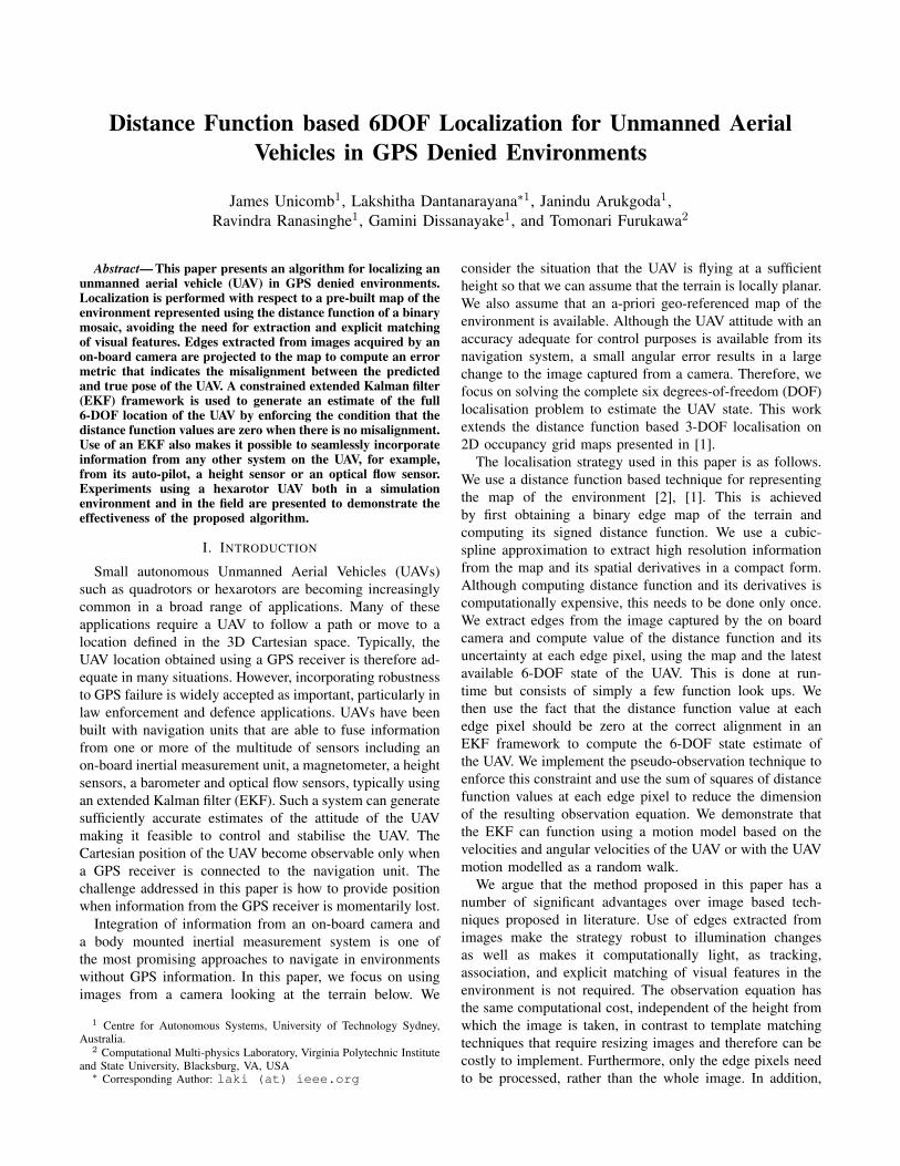
Fig. 2: Visual sensors mounted on the platform. (a). LiDar,Px4Flow and fisheye camera mounted on UAV . (b). Gimbalused to mount the perspective camera

(a) (b)

Fig. 3: (a) Map of the arena created by stitching UAV images.(b) Cleaned-up map used for localization.

to interface low level drivers and high-level algorithms suchas localisation.

IV. METHODOLOGY

A. Map of the Environment

In order to localise, the UAV uses a pre-built map repre-sented using the distance function of a binary mosaic thatcorrespond to the edges that are present in the environment.Fig. 3a shows the initial map built using the images acquiredusing the on board camera. This map has been pruned toremove spurious noise from the map while retaining theprominent edge image (Fig. 3b) to use as the final map.

B. Sensing the Environment

Once an image is captured through the on board camera(perspective camera or the fish-eye camera), it is processedto correct each pixel location for radial and tangential lensdistortions. Subsequently, the undistorted image is passed

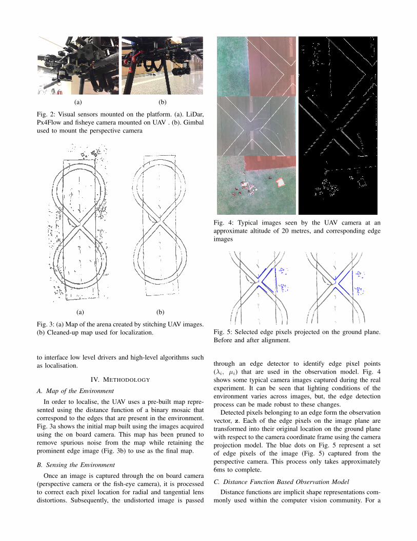
Fig. 4: Typical images seen by the UAV camera at anapproximate altitude of 20 metres, and corresponding edgeimages

Fig. 5: Selected edge pixels projected on the ground plane.Before and after alignment.

through an edge detector to identify edge pixel points(λi, µi) that are used in the observation model. Fig. 4shows some typical camera images captured during the realexperiment. It can be seen that lighting conditions of theenvironment varies across images, but, the edge detectionprocess can be made robust to these changes.

Detected pixels belonging to an edge form the observationvector, z. Each of the edge pixels on the image plane aretransformed into their original location on the ground planewith respect to the camera coordinate frame using the cameraprojection model. The blue dots on Fig. 5 represent a setof edge pixels of the image (Fig. 5) captured from theperspective camera. This process only takes approximately6ms to complete.

C. Distance Function Based Observation Model

Distance functions are implicit shape representations com-monly used within the computer vision community. For a

Fig. 6: Distance field of the arena

given binary image with the set of boundaries V , the distancefunction value at a given location x, is computed via (1),which specifies the Euclidean distance from that pixel to thenearest boundary pixel vj in V [9]. Fig. 6 shows the distancefield of the synthetically generated MBZIRC arena in Gazebosimulation environment.

DF (x) = minvj∈V

‖x− vj‖ (1)

The distance function as described in (1) quantises thesedistances into cell numbers. Furthermore, derivatives of thedistance functions are not continuous at points which belongto the edges of the binary map or to the cut-locus [10]. As thepurpose of the exercise is to use the distance functions as thebasis for an observation model within an EKF framework,a cubic spline approximation based interpolation algorithmis used to compute the distance function and its derivativesat any given location in the map. The parameters of thespline function are precomputed and stored so that thecomputational effort required during runtime is minimised.Future references to distance function in this paper refer tothe interpolated continuous version.

We further define the sign of the distance function basedon the colour of the initial binary map. Distances correspond-ing to points in black regions hold a positive value whilepoints in white region holds a negative value. This guaranteesthat the gradient of distance function is continuous at theedges of the binary map.

The observation vector zi ∈ z; zi = (λi, µi), of a singlebinary image obtained by the camera, consisting of n edgepoints with coordinates (λ, µ) on the image plane can beprojected from the current estimate of the 6DOF UAV posex = (x, y, z(altitude), ψ(roll), θ(pitch), φ(yaw))>, using(2) to obtain the observation vector in 2D space xo on theground plane.

xoi =

{xoiyoi

}=

{x+ z

λiR1,1+µiR1,2−fR1,3

λiR3,1−µiR3,2+fR3,3

y + zλiR2,1+µiR2,2−fR2,3

λiR3,1−µiR3,2+fR3,3

}(2)

where, R is the 3D rotation matrix representing the UAVpose, R(ψ, θ, φ), and f is the focal length of the camera.

When the projected edge points and the map are fullyaligned, the sum of squared distance function values at thesepoints is expected to be zero. Therefore, setting the expected

measurement to zero in (3) yields the measurement equation(4) that is suitable for robot localisation.

h(x, z) =

n−1∑i=0

DF (xoi)2 = dss (3)

h(x, z) = 0 (4)

D. Formulation of the Extended Kalman Filter

Traditional formulation of the EKF requires an observationequation of the form z = h(x). The alternative formulationthat is proposed below can directly deal with an implicit formof the measurement equation.

1) Prediction: Let the estimate of the UAV pose xk|k−1 =(xk|k−1, yk|k−1, zk|k−1, ψk|k−1, θk|k−1, φk|k−1)>, besubjected to a control command of uk = (vk, ωk)>, wherevk is the linear velocity (in x, y, and z directions) and ωk isthe angular velocity (in ψ, θ, and φ directions) over a periodof ∆t.

Then the predicted location of the UAV is given by (5)and its covariance by (6).

xk|k−1 = F (xk−1|k−1, uk∆t) (5)

Pk|k−1 = ∇FxPk−1|k−1∇F>x +∇FuQk∇F>u (6)

where ∇Fx and ∇Fu are respectively the Jacobian of thecontrol function F with respect to x and u, obtained bylinearising about the UAV pose estimate xk−1|k−1 , whileQk is the control noise covariance matrix.

2) Observation: Equation (4) provides the observationfunction, h(x, z) = 0.

Assuming that each selected pixel point of the edge imagez, corrupted by noise η with N (0, σ2) in both λ and µdirections, the covariance of the measurement vector is givenby the diagonal matrix, Σz = diag(σ2, σ2).

3) Update: Update equations can be written as follows,where the filter gain K is given by,

K = Pk|k−1∇h>x (∇hxPk|k−1∇h>x +∇hzΣz∇h>z )−1 (7)

The state update:

xk|k = xk|k−1 +K(−h(xk|k−1, z)) (8)

while the covariance update is,

Pk|k = (I −K∇hx)Pk|k−1 (9)

The Jacobians∇hx and∇hz at the appropriate linearisationpoints can be easily calculated using the DF .

As previously mentioned, DF and its derivatives can beprecomputed and stored to be used during the runtime toefficiently compute the gradients of DF and the Jacobiansabove. The remaining components of the gradient can thenbe analytically derived from (2).

Fig. 7: Flight path of the UAV during Gazebo simulation. Estimation without the use of odometry.

Fig. 8: Pose error and the relevant covariances during simu-lation without using odometry.

Fig. 4 and Fig. 5 shows spurious measurements resultingfrom the edge extraction process. This is to be expected in apractical situation as the objects that did not exist during themapping process can exist in the environment. Changes tothe illumination and shadows can also contribute to this. Aninnovation gate (with a 2σ bound) is used to rejects thesemeasurements before they reach the update stage.

V. EXPERIMENTAL RESULTS

In this section we validate the proposed algorithm usingsimulation and experimental data.

For simulations, we use the Gazebo robot simulationsoftware provided with ROS Kinetic Kame. The simulatedUAV flies at varying altitudes and captures images using amonocular camera that is mounted on the robot’s body. ThePixhawk controller firmware estimates the UAV velocitiesand odometry based on physics properties of the simulation.Ground-truth is known.

For the real experiment we used images obtained fromthe normal camera. The UAV is controlled by a PixhawkAutopilot device. RTK GPS unit is also present on the UAVand is used only for ground-truth. Map shown in Fig. 3b isused for localization.

A. Simulation Results

During the simulation, the UAV is flown in altitudesvarying between 20 - 40 metres and travels a total distanceof 1km. Fig. 7 shows a comparison between ground-truthand the estimated poses. Odometry generated from the UAVflight system is also plotted. This odometry is used withinthe EKF framework during the prediction phase. However, asthe flight system cannot estimate the x and y components ofthe UAV linear velocity in the absence of GPS, we considerthose components to be zero, and use a larger uncertainty tocapture the transition.

It can be seen that the estimation closely follows theground-truth trajectory. However, when the UAV moves outof the range of the arena (275 seconds into simulation,Fig. 8), the errors increase when the image captured by thecamera is completely blank, as soon as the UAV is back inrange, the estimate continues to track the trajectory well.

Fig. 9: Flight path of the UAV during the field trials.

B. Field Trials

Results from estimation during field trials are shown inFig. 9. Position updates from RTK-GPS system is onlyavailable at a 1Hz frequency and are plotted against theestimated pose. However, it is not reliable and dependson environment conditions. We use these GPS readings forground-truth purposes.

It can be seen that the estimates closely follow the ground-truth trajectory.

VI. CONCLUSION

In this paper, we presented an algorithm for localizinga UAV in absence of GPS signals. We use experimentsconducted both in simulation and field trials to demonstratethe effectiveness of the proposed algorithm. The resultsreported demonstrate that the estimated pose closely followground-truth trajectories even when an odometry estimate ofthe UAV is not present. It is also seen that the algorithmis able to reject observations from edges extracted from theimages that contain noise and artefacts that are not presentin the map.

Our future work will focus on incorporating informationfrom other sensors mounted on the UAV for example theoptical flow sensor. We also aim to explore the utility oftightly coupling the information from an IMU and othersensors in a single EKF framework.

One major limitation of the work presented is the as-sumption that the map of the environment that the UAVtraverses is planar. Relaxing this assumption using a full threedimensional distance map or exploring whether maintainingonly a planar map and relying on the outlier rejectioncapability of the EKF is adequate, are also of interest.

REFERENCES

[1] L. Dantanarayana, G. Dissanayake, R. Ranasinghe, andT. Furukawa, “An extended Kalman filter for localisationin occupancy grid maps,” in 2015 IEEE 10th InternationalConference on Industrial and Information Systems (ICIIS).IEEE, 12 2015, pp. 419–424. [Online]. Available:http://ieeexplore.ieee.org/lpdocs/epic03/wrapper.htm?arnumber=7399048

[2] L. Dantanarayana, G. Dissanayake, and R. Ranasinge,“C-LOG: A Chamfer Distance Based Algorithm forLocalisation in Occupancy Grid-maps,” CAAI Transactionson Intelligence Technology, 10 2016. [Online]. Available:http://linkinghub.elsevier.com/retrieve/pii/S2468232216300555

[3] A. Yol, B. Delabarre, A. Dame, J.-E. Dartois, and E. Marchand,“Vision-based absolute localization for unmanned aerial vehicles,”in 2014 IEEE/RSJ International Conference on Intelligent Robotsand Systems. IEEE, 9 2014, pp. 3429–3434. [Online]. Available:http://ieeexplore.ieee.org/document/6943040/

[4] O. Amidi, T. Kanade, and K. Fujita, “A visual odometer forautonomous helicopter flight,” Robotics and Autonomous Systems,vol. 28, no. 2-3, pp. 185–193, 8 1999. [Online]. Available:http://linkinghub.elsevier.com/retrieve/pii/S0921889099000160

[5] R. Madison, G. Andrews, P. DeBitetto, S. Rasmussen, andM. Bottkol, “Vision-Aided Navigation for Small UAVs in GPS-Challenged Environments,” in AIAA Infotech@Aerospace 2007Conference and Exhibit. Reston, Virigina: American Instituteof Aeronautics and Astronautics, 5 2007. [Online]. Available:http://arc.aiaa.org/doi/10.2514/6.2007-2986

[6] J. W. Langelaan, “State Estimation for Autonomous Flight inCluttered Environments,” Journal of Guidance, Control, andDynamics, vol. 30, no. 5, pp. 1414–1426, 9 2007. [Online]. Available:http://arc.aiaa.org/doi/10.2514/1.27770

[7] J. Yang, A. Dani, S.-J. Chung, and S. Hutchinson, “Inertial-AidedVision-Based Localization and Mapping in a Riverine Environmentwith Reflection Measurements,” in AIAA Guidance, Navigation, andControl (GNC) Conference. Reston, Virginia: American Instituteof Aeronautics and Astronautics, 8 2013. [Online]. Available:http://arc.aiaa.org/doi/10.2514/6.2013-5246

[8] Allen D. Wu, Eric N. Johnson, Michael Kaess, Frank Dellaert, andGirish Chowdhary, “Autonomous Flight in GPS-Denied EnvironmentsUsing Monocular Vision and Inertial Sensors,” Journal of AerospaceInformation Systems, vol. 10, no. 4, pp. 172–186, 4 2013. [Online].Available: http://arc.aiaa.org/doi/10.2514/1.I010023

[9] M. Y. Liu, O. Tuzel, A. Veeraraghavan, and R. Chellappa, “Fastdirectional chamfer matching,” in 2010 IEEE ComputerSociety Conference on Computer Vision and PatternRecognition. IEEE, 6 2010, pp. 1696–1703. [Online]. Available:http://ieeexplore.ieee.org/lpdocs/epic03/wrapper.htm?arnumber=5539837

[10] M. Jones, J. Baerentzen, and M. Sramek, “3D distance fields: a surveyof techniques and applications,” IEEE Transactions on Visualizationand Computer Graphics, vol. 12, no. 4, pp. 581–599, 7 2006.[Online]. Available: http://www.ncbi.nlm.nih.gov/pubmed/16805266http://ieeexplore.ieee.org/lpdocs/epic03/wrapper.htm?arnumber=1634323