Embed Size (px)
Citation preview

© 2015 H. Scott Hinton
Lesson: Robustness and Phenotype Phase Plane AnalysisBIE 5500/6500Utah State University
Constraint-based Metabolic Reconstructions & Analysis
Robustness Analysis & Phenotype Phase Plane Analysis
© 2015 H. Scott Hinton
Lesson: Robustness and Phenotype Phase Plane AnalysisBIE 5500/6500Utah State University
Constraint-based Metabolic Reconstructions & Analysis
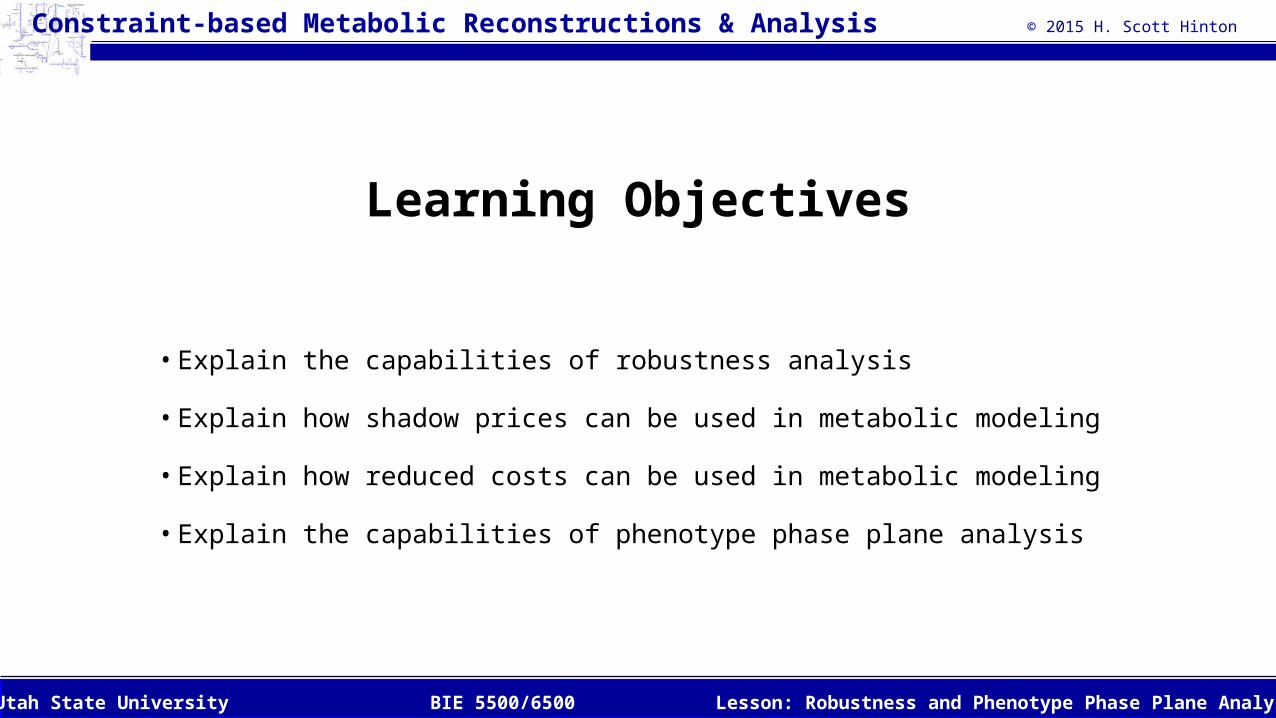
Learning Objectives
• Explain the capabilities of robustness analysis
• Explain how shadow prices can be used in metabolic modeling
• Explain how reduced costs can be used in metabolic modeling
• Explain the capabilities of phenotype phase plane analysis

© 2015 H. Scott Hinton
Lesson: Robustness and Phenotype Phase Plane AnalysisBIE 5500/6500Utah State University
Constraint-based Metabolic Reconstructions & Analysis
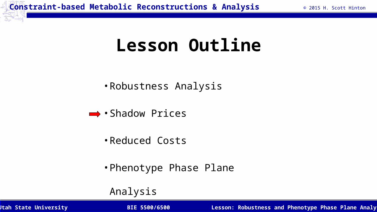
Lesson Outline
• Robustness Analysis
• Shadow Prices
• Reduced Costs
• Phenotype Phase Plane
Analysis
© 2015 H. Scott Hinton
Lesson: Robustness and Phenotype Phase Plane AnalysisBIE 5500/6500Utah State University
Constraint-based Metabolic Reconstructions & Analysis
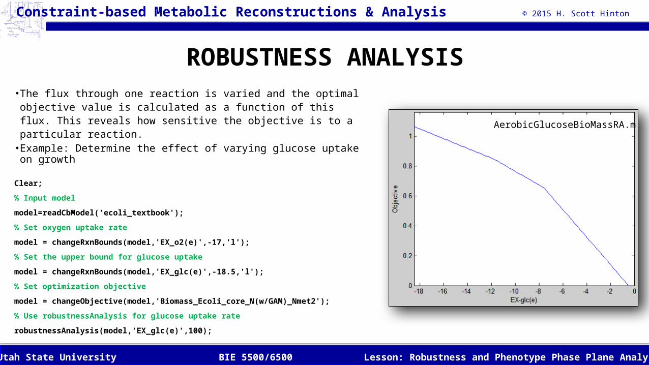
ROBUSTNESS ANALYSIS• The flux through one reaction is varied and the optimal
objective value is calculated as a function of this flux. This reveals how sensitive the objective is to a particular reaction.
• Example: Determine the effect of varying glucose uptake on growth
Clear;
% Input model
model=readCbModel('ecoli_textbook');
% Set oxygen uptake rate
model = changeRxnBounds(model,'EX_o2(e)',-17,'l');
% Set the upper bound for glucose uptake
model = changeRxnBounds(model,'EX_glc(e)',-18.5,'l');
% Set optimization objective
model = changeObjective(model,'Biomass_Ecoli_core_N(w/GAM)_Nmet2');
% Use robustnessAnalysis for glucose uptake rate
robustnessAnalysis(model,'EX_glc(e)',100);
AerobicGlucoseBioMassRA.m
© 2015 H. Scott Hinton
Lesson: Robustness and Phenotype Phase Plane AnalysisBIE 5500/6500Utah State University
Constraint-based Metabolic Reconstructions & Analysis
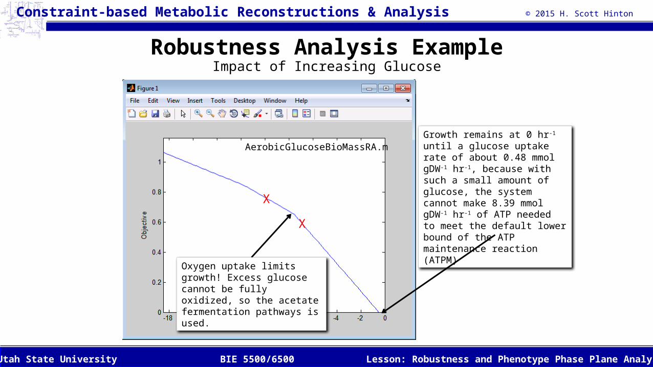
Robustness Analysis ExampleImpact of Increasing Glucose
Growth remains at 0 hr-1 until a glucose uptake rate of about 0.48 mmol gDW-1 hr-1, because with such a small amount of glucose, the system cannot make 8.39 mmol gDW-1 hr-1 of ATP needed to meet the default lower bound of the ATP maintenance reaction (ATPM)
Oxygen uptake limits growth! Excess glucose cannot be fully oxidized, so the acetate fermentation pathways is used.
X
X
AerobicGlucoseBioMassRA.m
© 2015 H. Scott Hinton
Lesson: Robustness and Phenotype Phase Plane AnalysisBIE 5500/6500Utah State University
Constraint-based Metabolic Reconstructions & Analysis
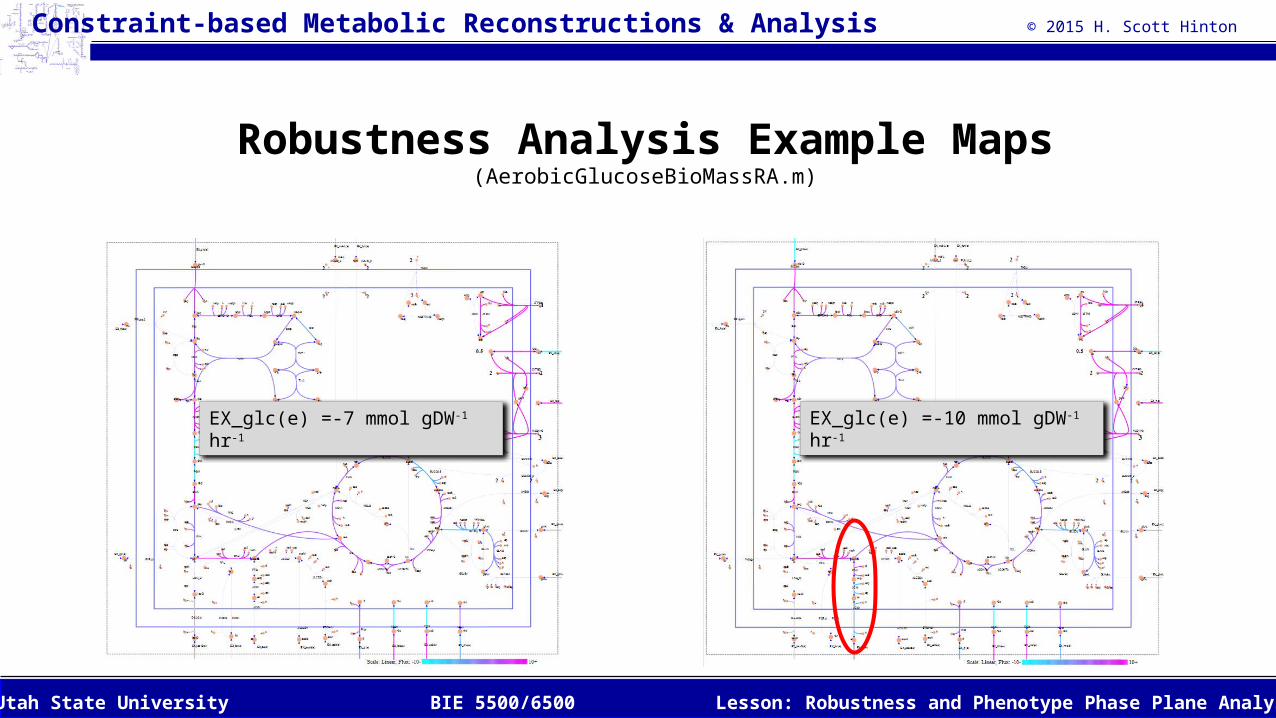
Robustness Analysis Example Maps(AerobicGlucoseBioMassRA.m)
EX_glc(e) =-7 mmol gDW-1 hr-1 EX_glc(e) =-10 mmol gDW-1 hr-1
© 2015 H. Scott Hinton
Lesson: Robustness and Phenotype Phase Plane AnalysisBIE 5500/6500Utah State University
Constraint-based Metabolic Reconstructions & Analysis
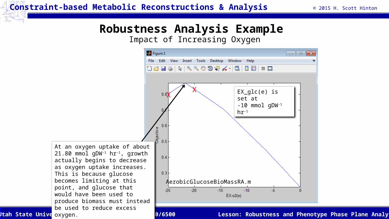
Robustness Analysis Example Impact of Increasing Oxygen
At an oxygen uptake of about 21.80 mmol gDW-1 hr-1, growth actually begins to decrease as oxygen uptake increases. This is because glucose becomes limiting at this point, and glucose that would have been used to produce biomass must instead be used to reduce excess oxygen.
EX_glc(e) is set at -10 mmol gDW-1 hr-1
AerobicGlucoseBioMassRA.m
XX
© 2015 H. Scott Hinton
Lesson: Robustness and Phenotype Phase Plane AnalysisBIE 5500/6500Utah State University
Constraint-based Metabolic Reconstructions & Analysis
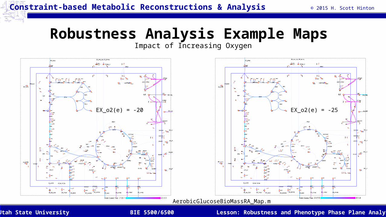
Robustness Analysis Example Maps Impact of Increasing Oxygen
EX_o2(e) = -20 EX_o2(e) = -25
AerobicGlucoseBioMassRA_Map.m
© 2015 H. Scott Hinton
Lesson: Robustness and Phenotype Phase Plane AnalysisBIE 5500/6500Utah State University
Constraint-based Metabolic Reconstructions & Analysis
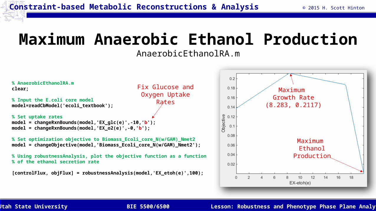
Maximum Anaerobic Ethanol ProductionAnaerobicEthanolRA.m
% AnaerobicEthanolRA.mclear;
% Input the E.coli core modelmodel=readCbModel('ecoli_textbook');
% Set uptake ratesmodel = changeRxnBounds(model,'EX_glc(e)',-10,‘b'); model = changeRxnBounds(model,'EX_o2(e)',-0,'b');
% Set optimization objective to Biomass_Ecoli_core_N(w/GAM)_Nmet2model = changeObjective(model,'Biomass_Ecoli_core_N(w/GAM)_Nmet2');
% Using robustnessAnalysis, plot the objective function as a function % of the ethanol secretion rate
[controlFlux, objFlux] = robustnessAnalysis(model,'EX_etoh(e)',100);
Maximum Growth Rate
(8.283, 0.2117)
Maximum Ethanol
Production
Fix Glucose and Oxygen Uptake
Rates
© 2015 H. Scott Hinton
Lesson: Robustness and Phenotype Phase Plane AnalysisBIE 5500/6500Utah State University
Constraint-based Metabolic Reconstructions & Analysis
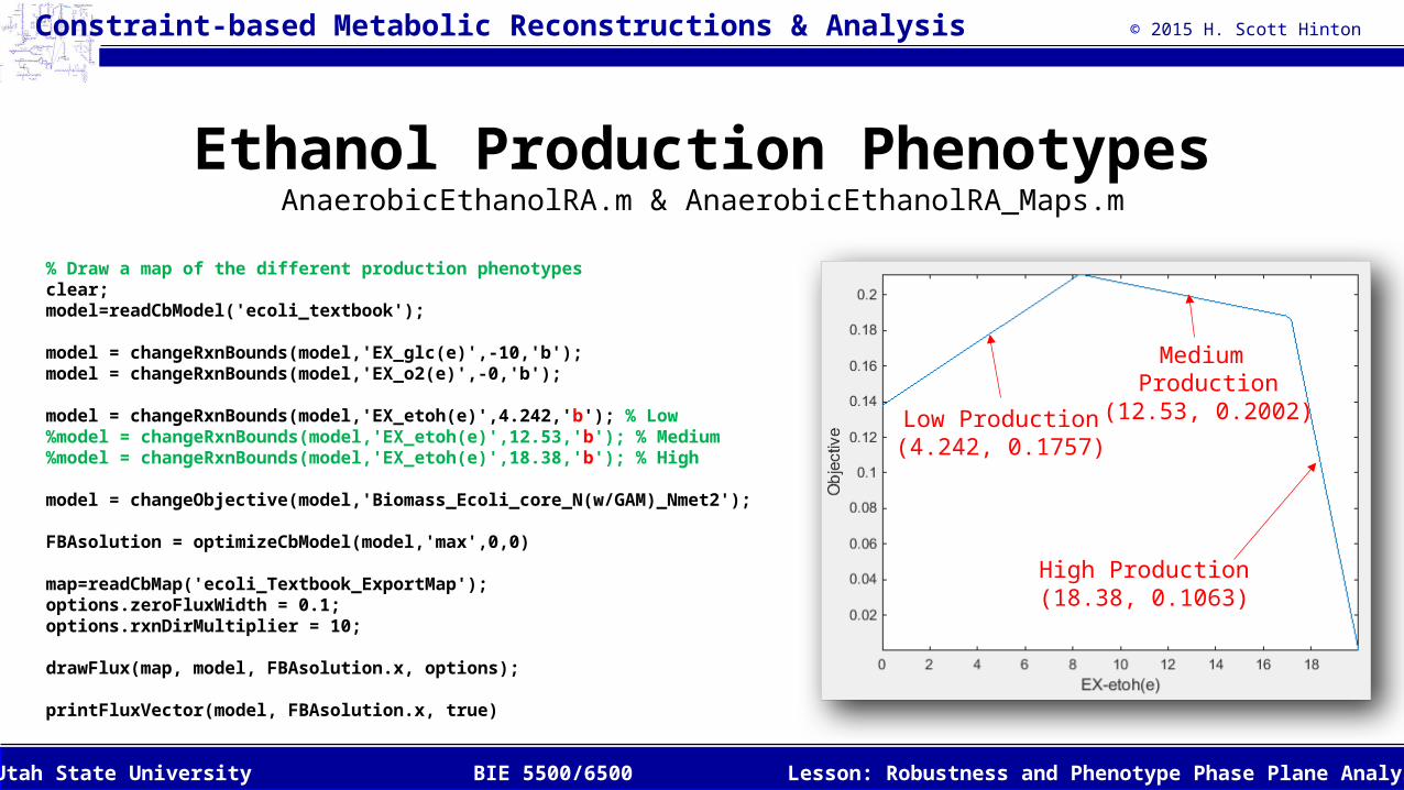
Ethanol Production PhenotypesAnaerobicEthanolRA.m & AnaerobicEthanolRA_Maps.m
% Draw a map of the different production phenotypesclear;model=readCbModel('ecoli_textbook');
model = changeRxnBounds(model,'EX_glc(e)',-10,'b'); model = changeRxnBounds(model,'EX_o2(e)',-0,'b');
model = changeRxnBounds(model,'EX_etoh(e)',4.242,'b'); % Low %model = changeRxnBounds(model,'EX_etoh(e)',12.53,'b'); % Medium %model = changeRxnBounds(model,'EX_etoh(e)',18.38,'b'); % High
model = changeObjective(model,'Biomass_Ecoli_core_N(w/GAM)_Nmet2');
FBAsolution = optimizeCbModel(model,'max',0,0)
map=readCbMap('ecoli_Textbook_ExportMap');options.zeroFluxWidth = 0.1;options.rxnDirMultiplier = 10;
drawFlux(map, model, FBAsolution.x, options);
printFluxVector(model, FBAsolution.x, true)
Low Production(4.242, 0.1757)
High Production(18.38, 0.1063)
Medium Production
(12.53, 0.2002)
© 2015 H. Scott Hinton
Lesson: Robustness and Phenotype Phase Plane AnalysisBIE 5500/6500Utah State University
Constraint-based Metabolic Reconstructions & Analysis
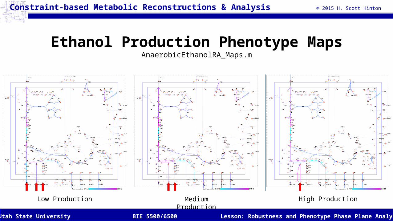
Ethanol Production Phenotype MapsAnaerobicEthanolRA_Maps.m
Low Production Medium Production High Production
© 2015 H. Scott Hinton
Lesson: Robustness and Phenotype Phase Plane AnalysisBIE 5500/6500Utah State University
Constraint-based Metabolic Reconstructions & Analysis
Lesson Outline
• Robustness Analysis
• Shadow Prices
• Reduced Costs
• Phenotype Phase Plane
Analysis
© 2015 H. Scott Hinton
Lesson: Robustness and Phenotype Phase Plane AnalysisBIE 5500/6500Utah State University
Constraint-based Metabolic Reconstructions & Analysis
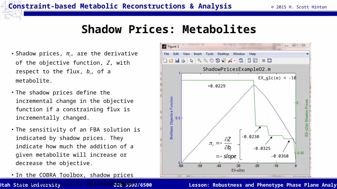
Shadow Prices: Metabolites
• Shadow prices, πi, are the derivative of the
objective function, Z, with respect to the flux,
bi, of a metabolite.
• The shadow prices define the incremental
change in the objective function if a
constraining flux is incrementally changed.
• The sensitivity of an FBA solution is indicated
by shadow prices. They indicate how much
the addition of a given metabolite will
increase or decrease the objective.
• In the COBRA Toolbox, shadow prices can be
calculated by optimizeCbModel. The vector
of y shadow prices is solution.y (glpk
solver)
-0.0360
-0.0325
-0.0230
+0.0229
ii
Z
b
slope
ShadowPricesExampleO2.m
EX_glc(e) = -10
© 2015 H. Scott Hinton
Lesson: Robustness and Phenotype Phase Plane AnalysisBIE 5500/6500Utah State University
Constraint-based Metabolic Reconstructions & Analysis
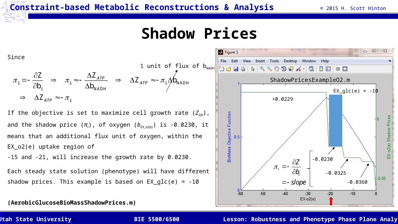
Shadow PricesSince
If the objective is set to maximize cell growth rate (ZGR), and the
shadow price (πi), of oxygen (bEX_o2(e)) is -0.0230, it means that an
additional flux unit of oxygen, within the EX_o2(e) uptake region
of
-15 and -21, will increase the growth rate by 0.0230.
Each steady state solution (phenotype) will have different
shadow prices. This example is based on EX_glc(e) = -10
(AerobicGlucoseBioMassShadowPrices.m)
i i i NADHi NADH
i
Z ZZ b
b b
Z
ATPATP
ATP
1 unit of flux of bNADH
-0.0360
-0.0325
-0.0230
+0.0229
ii
Z
b
slope
EX_glc(e) = -10
ShadowPricesExampleO2.m
© 2015 H. Scott Hinton
Lesson: Robustness and Phenotype Phase Plane AnalysisBIE 5500/6500Utah State University
Constraint-based Metabolic Reconstructions & Analysis
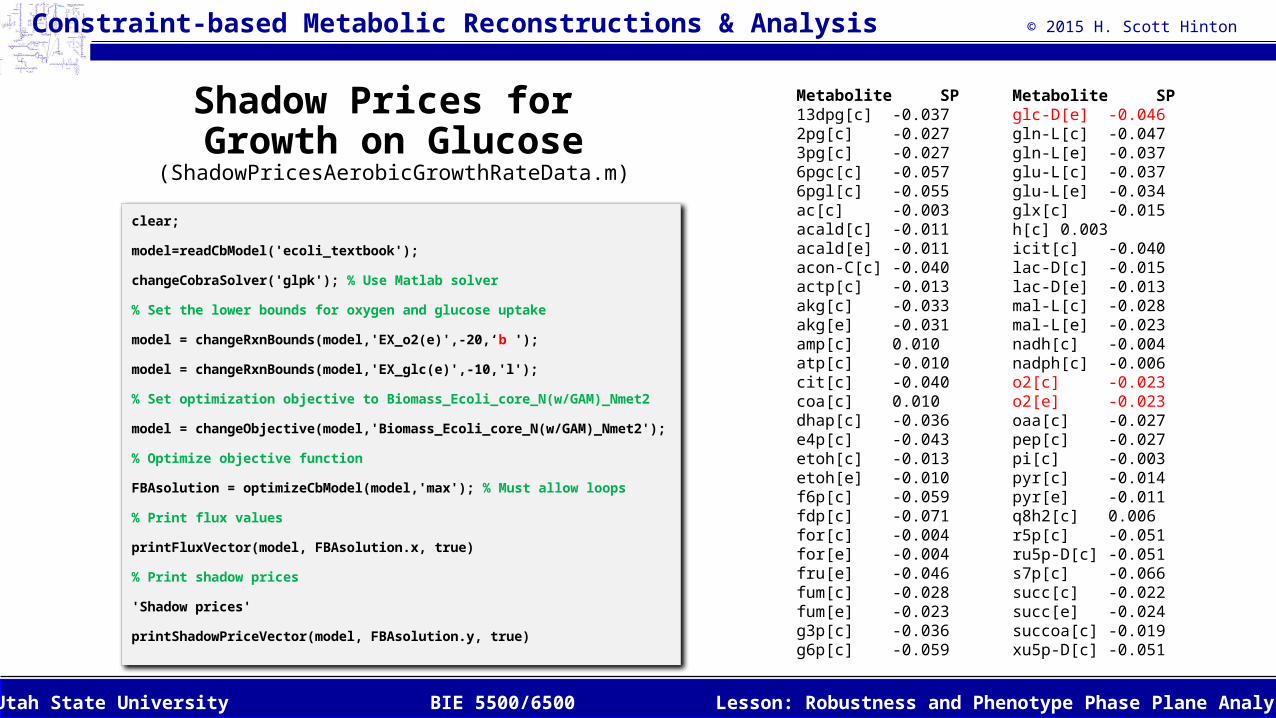
Shadow Prices for Growth on Glucose
(ShadowPricesAerobicGrowthRateData.m)
clear;
model=readCbModel('ecoli_textbook');
changeCobraSolver('glpk'); % Use Matlab solver
% Set the lower bounds for oxygen and glucose uptake
model = changeRxnBounds(model,'EX_o2(e)',-20,‘b ');
model = changeRxnBounds(model,'EX_glc(e)',-10,'l');
% Set optimization objective to Biomass_Ecoli_core_N(w/GAM)_Nmet2
model =
changeObjective(model,'Biomass_Ecoli_core_N(w/GAM)_Nmet2');
% Optimize objective function
FBAsolution = optimizeCbModel(model,'max'); % Must allow loops
% Print flux values
printFluxVector(model, FBAsolution.x, true)
% Print shadow prices
'Shadow prices'
printShadowPriceVector(model, FBAsolution.y, true)
Metabolite SP13dpg[c] -0.0372pg[c] -0.0273pg[c] -0.0276pgc[c] -0.0576pgl[c] -0.055ac[c] -0.003acald[c] -0.011acald[e] -0.011acon-C[c] -0.040actp[c] -0.013akg[c] -0.033akg[e] -0.031amp[c] 0.010atp[c] -0.010cit[c] -0.040coa[c] 0.010dhap[c] -0.036e4p[c] -0.043etoh[c] -0.013etoh[e] -0.010f6p[c] -0.059fdp[c] -0.071for[c] -0.004for[e] -0.004fru[e] -0.046fum[c] -0.028fum[e] -0.023g3p[c] -0.036g6p[c] -0.059
Metabolite SPglc-D[e] -0.046gln-L[c] -0.047gln-L[e] -0.037glu-L[c] -0.037glu-L[e] -0.034glx[c] -0.015h[c] 0.003icit[c] -0.040lac-D[c] -0.015lac-D[e] -0.013mal-L[c] -0.028mal-L[e] -0.023nadh[c] -0.004nadph[c] -0.006o2[c] -0.023o2[e] -0.023oaa[c] -0.027pep[c] -0.027pi[c] -0.003pyr[c] -0.014pyr[e] -0.011q8h2[c] 0.006r5p[c] -0.051ru5p-D[c] -0.051s7p[c] -0.066succ[c] -0.022succ[e] -0.024succoa[c] -0.019xu5p-D[c] -0.051
© 2015 H. Scott Hinton
Lesson: Robustness and Phenotype Phase Plane AnalysisBIE 5500/6500Utah State University
Constraint-based Metabolic Reconstructions & Analysis
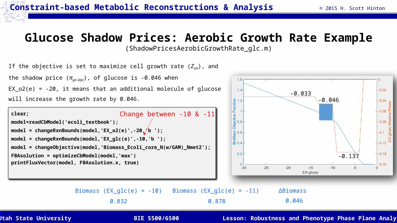
Glucose Shadow Prices: Aerobic Growth Rate Example(ShadowPricesAerobicGrowthRate_glc.m)
If the objective is set to maximize cell growth rate (ZGR), and the
shadow price (πglc-D[e]), of glucose is -0.046 when
EX_o2(e) = -20, it means that an additional molecule of glucose will
increase the growth rate by 0.046.
clear;
model=readCbModel('ecoli_textbook');
model = changeRxnBounds(model,'EX_o2(e)',-20,‘b ');
model = changeRxnBounds(model,'EX_glc(e)',-10,‘b ');
model = changeObjective(model,'Biomass_Ecoli_core_N(w/GAM)_Nmet2');
FBAsolution = optimizeCbModel(model,'max')printFluxVector(model, FBAsolution.x, true)
Biomass (EX_glc(e) = -10)
0.832 0.878
Biomass (EX_glc(e) = -11) ΔBiomass
0.046
-0.046
-0.137
-0.033
Change between -10 & -11
© 2015 H. Scott Hinton
Lesson: Robustness and Phenotype Phase Plane AnalysisBIE 5500/6500Utah State University
Constraint-based Metabolic Reconstructions & Analysis
Lesson Outline
• Robustness Analysis
• Shadow Prices
• Reduced Costs
• Phenotype Phase Plane
Analysis
© 2015 H. Scott Hinton
Lesson: Robustness and Phenotype Phase Plane AnalysisBIE 5500/6500Utah State University
Constraint-based Metabolic Reconstructions & Analysis
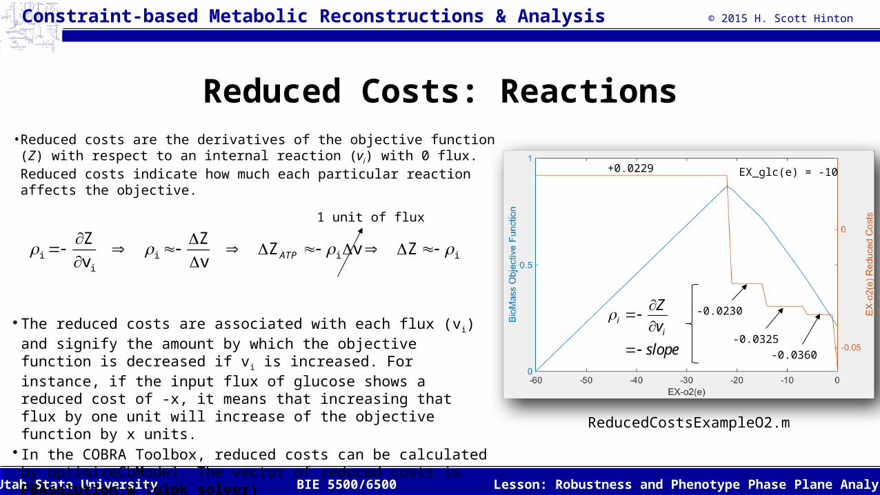
Reduced Costs: Reactions• Reduced costs are the derivatives of the objective function (Z) with respect to an internal reaction (vi) with 0 flux. Reduced costs indicate how much each particular reaction affects the objective.
• The reduced costs are associated with each flux (vi) and signify the amount by which the objective function is decreased if vi is increased. For instance, if the input flux of glucose shows a reduced cost of -x, it means that increasing that flux by one unit will increase of the objective function by x units.
• In the COBRA Toolbox, reduced costs can be calculated by optimizeCbModel. The vector of reduced costs is FBAsolution.w (glpk solver)
i i i ii
Z ZZ v Z
v v ATP
1 unit of flux
EX_glc(e) = -10+0.0229
-0.0230
-0.0325-0.0360
ii
Z
v
slope
ReducedCostsExampleO2.m
© 2015 H. Scott Hinton
Lesson: Robustness and Phenotype Phase Plane AnalysisBIE 5500/6500Utah State University
Constraint-based Metabolic Reconstructions & Analysis
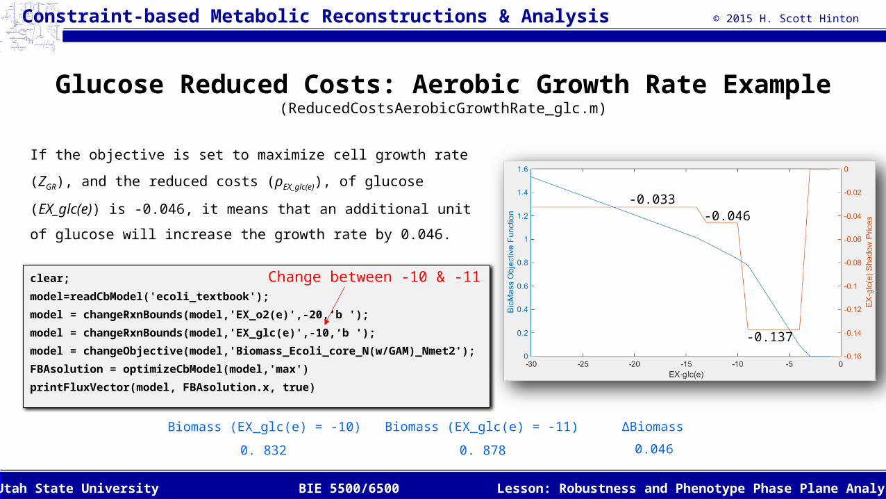
Glucose Reduced Costs: Aerobic Growth Rate Example(ReducedCostsAerobicGrowthRate_glc.m)
If the objective is set to maximize cell growth rate
(ZGR), and the reduced costs (ρEX_glc(e)), of glucose
(EX_glc(e)) is -0.046, it means that an additional unit
of glucose will increase the growth rate by 0.046.
clear;
model=readCbModel('ecoli_textbook');
model = changeRxnBounds(model,'EX_o2(e)',-20,‘b ');
model = changeRxnBounds(model,'EX_glc(e)',-10,‘b ');
model = changeObjective(model,'Biomass_Ecoli_core_N(w/GAM)_Nmet2');
FBAsolution = optimizeCbModel(model,'max')
printFluxVector(model, FBAsolution.x, true)
Biomass (EX_glc(e) = -10)
0. 832 0. 878
Biomass (EX_glc(e) = -11) ΔBiomass
0.046
-0.046
-0.137
-0.033
Change between -10 & -11
© 2015 H. Scott Hinton
Lesson: Robustness and Phenotype Phase Plane AnalysisBIE 5500/6500Utah State University
Constraint-based Metabolic Reconstructions & Analysis
Lesson Outline
• Robustness Analysis
• Shadow Prices
• Reduced Costs
• Phenotype Phase Plane
Analysis
© 2015 H. Scott Hinton
Lesson: Robustness and Phenotype Phase Plane AnalysisBIE 5500/6500Utah State University
Constraint-based Metabolic Reconstructions & Analysis
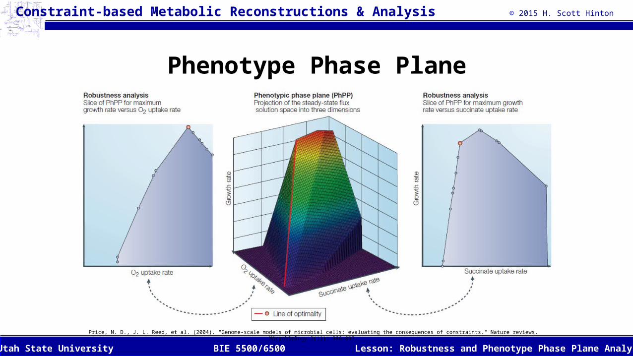
Phenotype Phase Plane
Price, N. D., J. L. Reed, et al. (2004). "Genome-scale models of microbial cells: evaluating the consequences of constraints." Nature reviews. Microbiology 2(11): 886-897.
© 2015 H. Scott Hinton
Lesson: Robustness and Phenotype Phase Plane AnalysisBIE 5500/6500Utah State University
Constraint-based Metabolic Reconstructions & Analysis
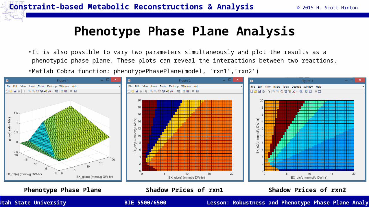
Phenotype Phase Plane Analysis
• It is also possible to vary two parameters simultaneously and plot the results as a phenotypic phase plane. These plots can reveal the interactions between two reactions.
• Matlab Cobra function: phenotypePhasePlane(model, ‘rxn1’,’rxn2’)
Phenotype Phase Plane Shadow Prices of rxn1 Shadow Prices of rxn2
© 2015 H. Scott Hinton
Lesson: Robustness and Phenotype Phase Plane AnalysisBIE 5500/6500Utah State University
Constraint-based Metabolic Reconstructions & Analysis
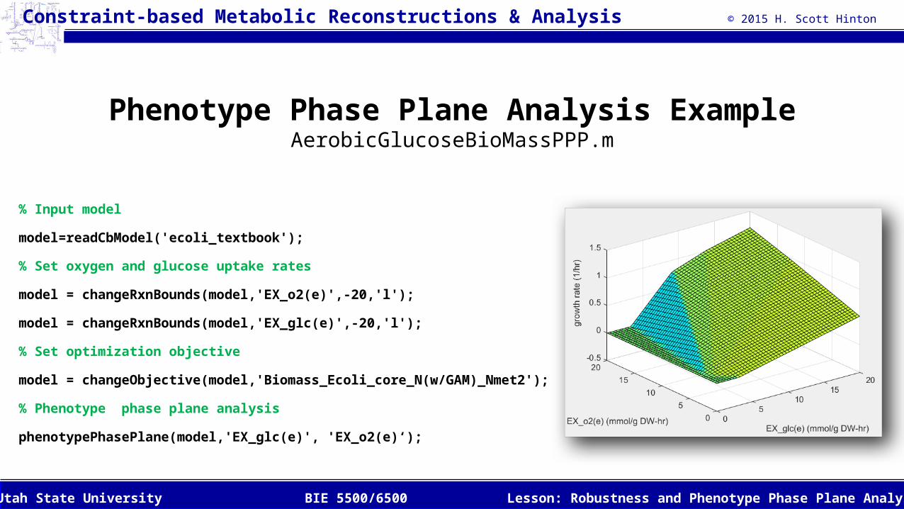
Phenotype Phase Plane Analysis ExampleAerobicGlucoseBioMassPPP.m
% Input model
model=readCbModel('ecoli_textbook');
% Set oxygen and glucose uptake rates
model = changeRxnBounds(model,'EX_o2(e)',-20,'l');
model = changeRxnBounds(model,'EX_glc(e)',-20,'l');
% Set optimization objective
model = changeObjective(model,'Biomass_Ecoli_core_N(w/GAM)_Nmet2');
% Phenotype phase plane analysis
phenotypePhasePlane(model,'EX_glc(e)', 'EX_o2(e)‘);
© 2015 H. Scott Hinton
Lesson: Robustness and Phenotype Phase Plane AnalysisBIE 5500/6500Utah State University
Constraint-based Metabolic Reconstructions & Analysis
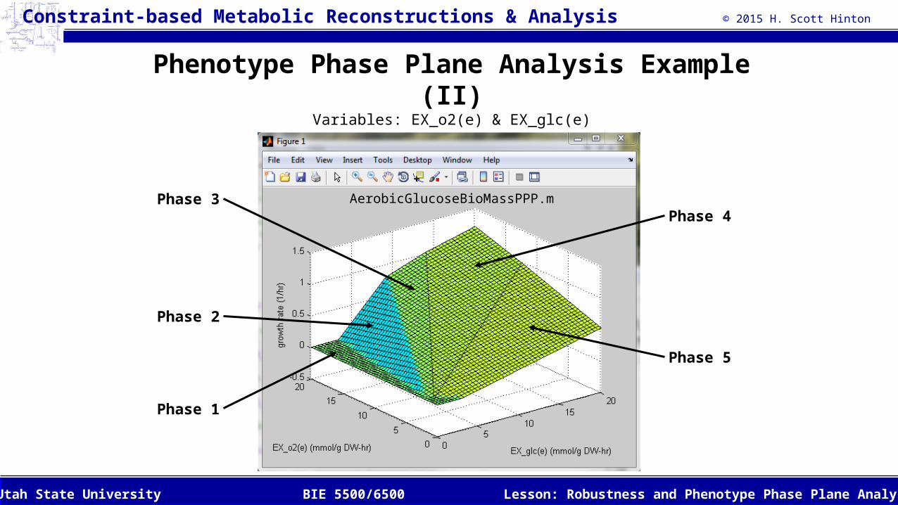
Phenotype Phase Plane Analysis Example (II)
Variables: EX_o2(e) & EX_glc(e)
Phase 1
Phase 3
Phase 2
Phase 4
Phase 5
AerobicGlucoseBioMassPPP.m
© 2015 H. Scott Hinton
Lesson: Robustness and Phenotype Phase Plane AnalysisBIE 5500/6500Utah State University
Constraint-based Metabolic Reconstructions & Analysis
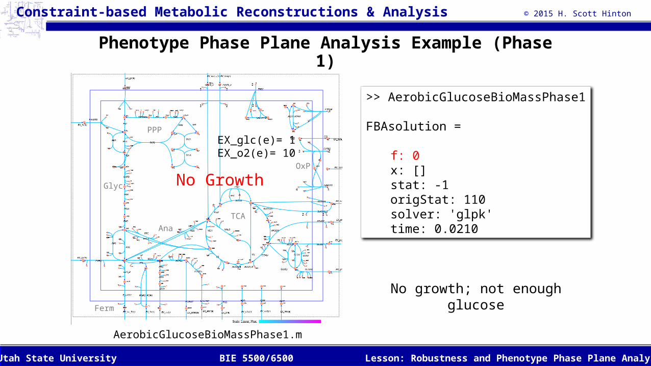
Phenotype Phase Plane Analysis Example (Phase 1)
>> AerobicGlucoseBioMassPhase1
FBAsolution =
f: 0x: []stat: -1origStat: 110solver: 'glpk'time: 0.0210
No Growth
No growth; not enough glucose
AerobicGlucoseBioMassPhase1.m
EX_glc(e)= 1EX_o2(e)= 10
Ferm
TCA
PPP
Glyc
Ana
OxP
© 2015 H. Scott Hinton
Lesson: Robustness and Phenotype Phase Plane AnalysisBIE 5500/6500Utah State University
Constraint-based Metabolic Reconstructions & Analysis
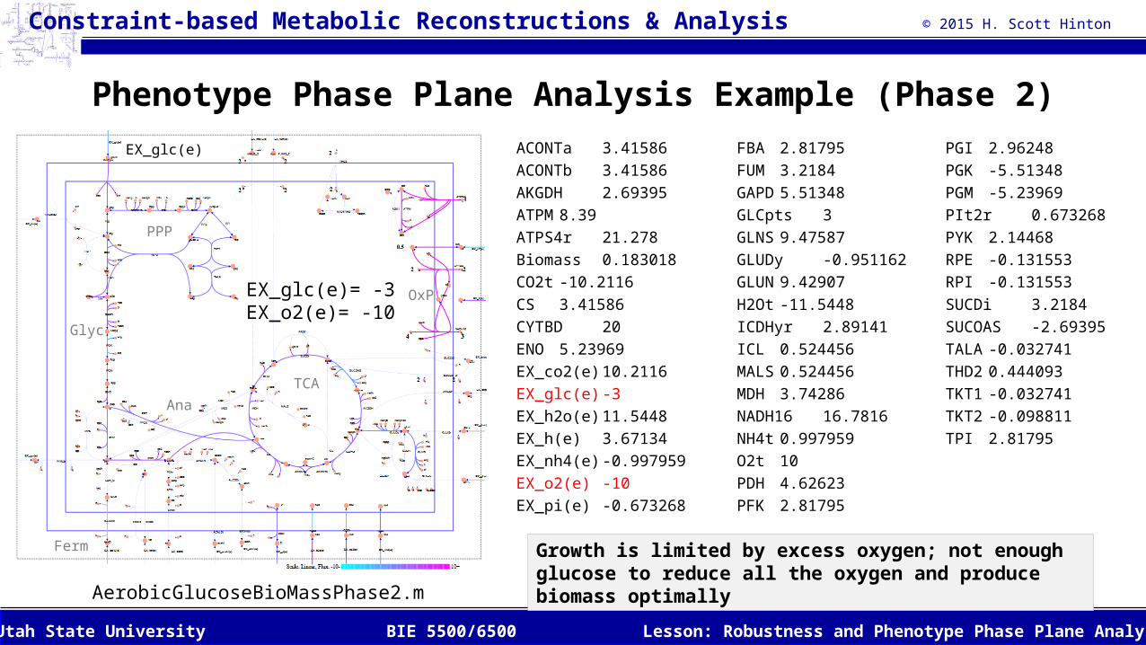
Phenotype Phase Plane Analysis Example (Phase 2)
ACONTa 3.41586ACONTb 3.41586AKGDH 2.69395ATPM 8.39ATPS4r 21.278Biomass 0.183018CO2t -10.2116CS 3.41586CYTBD 20ENO 5.23969EX_co2(e) 10.2116EX_glc(e) -3EX_h2o(e) 11.5448EX_h(e) 3.67134EX_nh4(e) -0.997959EX_o2(e) -10EX_pi(e) -0.673268
AerobicGlucoseBioMassPhase2.m
EX_glc(e)
Growth is limited by excess oxygen; not enough glucose to reduce all the oxygen and produce biomass optimally
FBA 2.81795FUM 3.2184GAPD 5.51348GLCpts 3GLNS 9.47587GLUDy -0.951162GLUN 9.42907H2Ot -11.5448ICDHyr 2.89141ICL 0.524456MALS 0.524456MDH 3.74286NADH16 16.7816NH4t 0.997959O2t 10PDH 4.62623PFK 2.81795
EX_glc(e)= -3EX_o2(e)= -10
PGI 2.96248PGK -5.51348PGM -5.23969PIt2r 0.673268PYK 2.14468RPE -0.131553RPI -0.131553SUCDi 3.2184SUCOAS -2.69395TALA -0.032741THD2 0.444093TKT1 -0.032741TKT2 -0.098811TPI 2.81795
Ferm
TCA
PPP
Glyc
Ana
OxP
© 2015 H. Scott Hinton
Lesson: Robustness and Phenotype Phase Plane AnalysisBIE 5500/6500Utah State University
Constraint-based Metabolic Reconstructions & Analysis
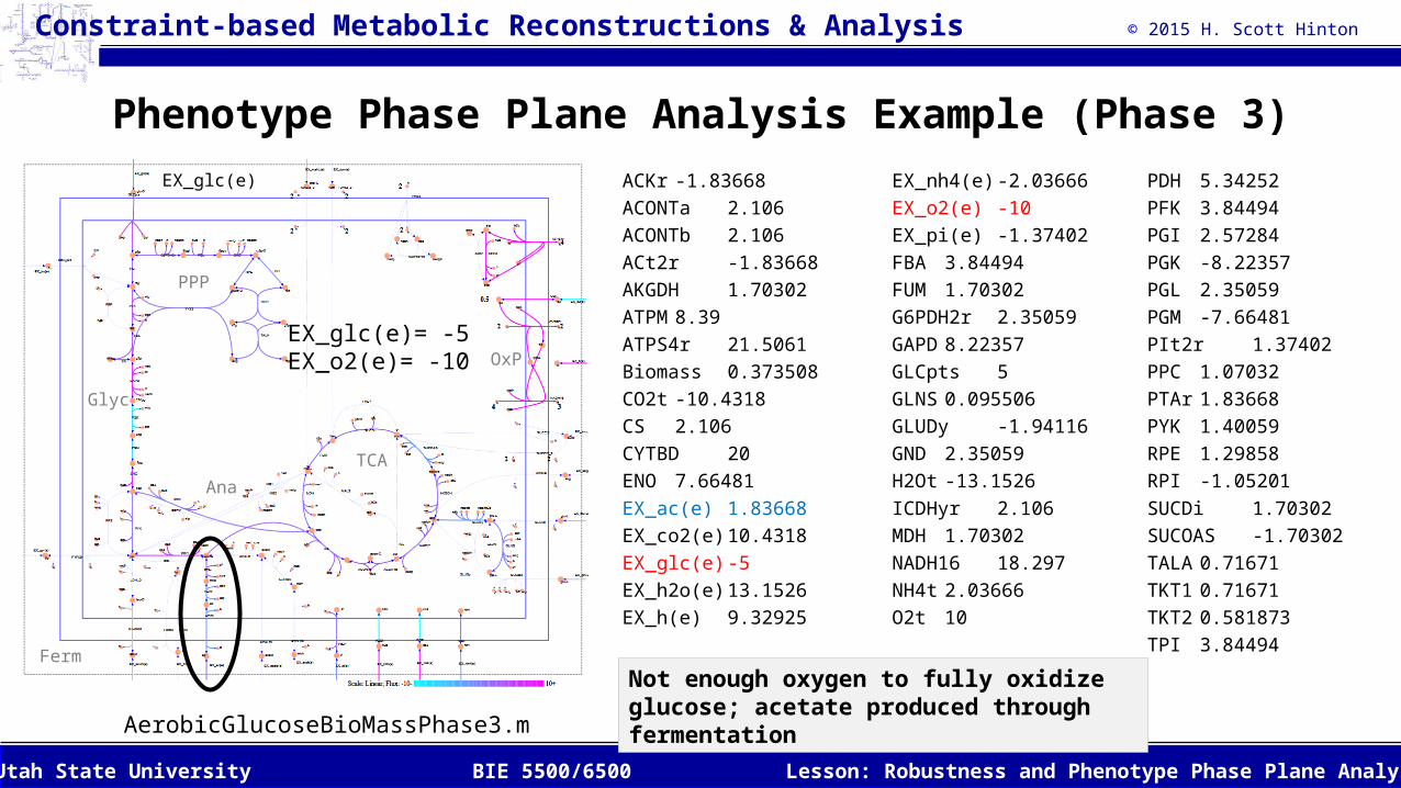
Phenotype Phase Plane Analysis Example (Phase 3)
ACKr -1.83668ACONTa 2.106ACONTb 2.106ACt2r -1.83668AKGDH 1.70302ATPM 8.39ATPS4r 21.5061Biomass 0.373508CO2t -10.4318CS 2.106CYTBD 20ENO 7.66481EX_ac(e) 1.83668EX_co2(e) 10.4318EX_glc(e) -5EX_h2o(e) 13.1526EX_h(e) 9.32925
AerobicGlucoseBioMassPhase3.m
EX_nh4(e) -2.03666EX_o2(e) -10EX_pi(e) -1.37402FBA 3.84494FUM 1.70302G6PDH2r 2.35059GAPD 8.22357GLCpts 5GLNS 0.095506GLUDy -1.94116GND 2.35059H2Ot -13.1526ICDHyr 2.106MDH 1.70302NADH16 18.297NH4t 2.03666O2t 10
PDH 5.34252PFK 3.84494PGI 2.57284PGK -8.22357PGL 2.35059PGM -7.66481PIt2r 1.37402PPC 1.07032PTAr 1.83668PYK 1.40059RPE 1.29858RPI -1.05201SUCDi 1.70302SUCOAS -1.70302TALA 0.71671TKT1 0.71671TKT2 0.581873TPI 3.84494
EX_glc(e)
EX_glc(e)= -3EX_o2(e)= -10
EX_glc(e)
Ferm
TCA
PPP
Glyc
Ana
OxP
Not enough oxygen to fully oxidize glucose; acetate produced through fermentation
EX_glc(e)= -5EX_o2(e)= -10
© 2015 H. Scott Hinton
Lesson: Robustness and Phenotype Phase Plane AnalysisBIE 5500/6500Utah State University
Constraint-based Metabolic Reconstructions & Analysis
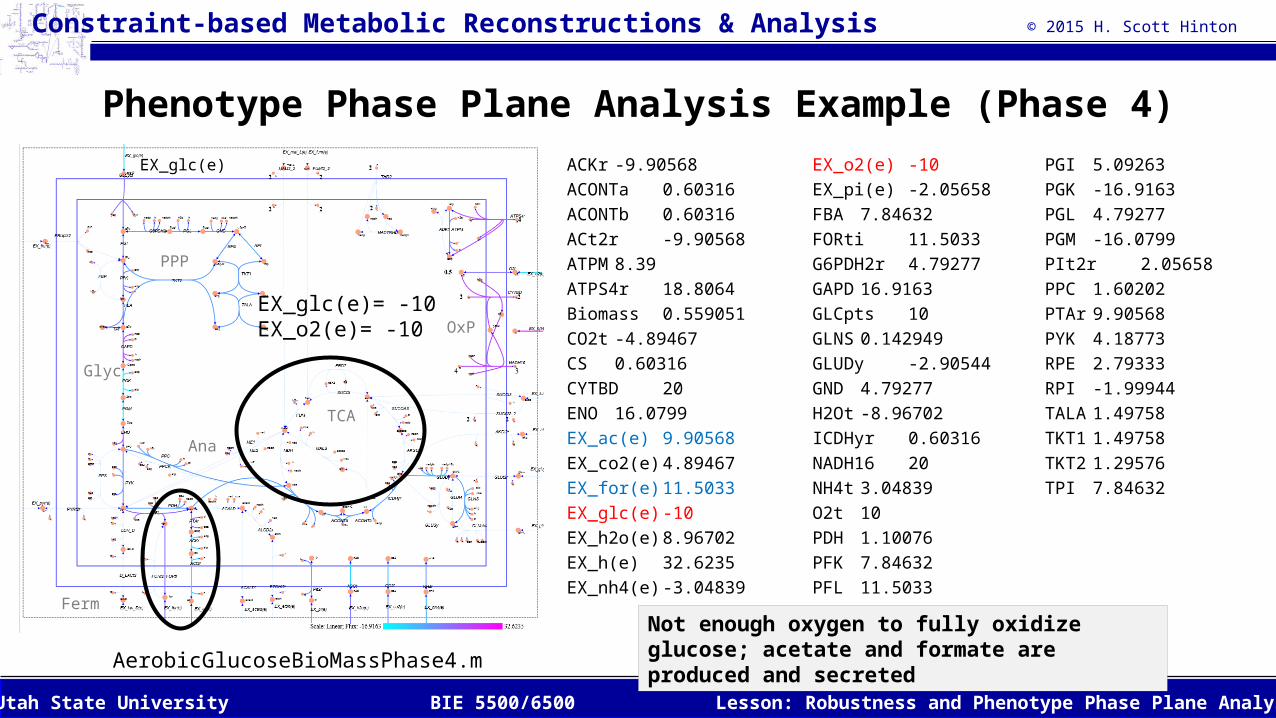
Phenotype Phase Plane Analysis Example (Phase 4)
ACKr -9.90568ACONTa 0.60316ACONTb 0.60316ACt2r -9.90568ATPM 8.39ATPS4r 18.8064Biomass 0.559051CO2t -4.89467CS 0.60316CYTBD 20ENO 16.0799EX_ac(e) 9.90568EX_co2(e) 4.89467EX_for(e) 11.5033EX_glc(e) -10EX_h2o(e) 8.96702EX_h(e) 32.6235EX_nh4(e) -3.04839
AerobicGlucoseBioMassPhase4.m
EX_o2(e) -10EX_pi(e) -2.05658FBA 7.84632FORti 11.5033G6PDH2r 4.79277GAPD 16.9163GLCpts 10GLNS 0.142949GLUDy -2.90544GND 4.79277H2Ot -8.96702ICDHyr 0.60316NADH16 20NH4t 3.04839O2t 10PDH 1.10076PFK 7.84632PFL 11.5033
PGI 5.09263PGK -16.9163PGL 4.79277PGM -16.0799PIt2r 2.05658PPC 1.60202PTAr 9.90568PYK 4.18773RPE 2.79333RPI -1.99944TALA 1.49758TKT1 1.49758TKT2 1.29576TPI 7.84632
EX_glc(e)
Ferm
TCA
PPP
Glyc
Ana
OxPEX_glc(e)= -10EX_o2(e)= -10
Not enough oxygen to fully oxidize glucose; acetate and formate are produced and secreted
© 2015 H. Scott Hinton
Lesson: Robustness and Phenotype Phase Plane AnalysisBIE 5500/6500Utah State University
Constraint-based Metabolic Reconstructions & Analysis
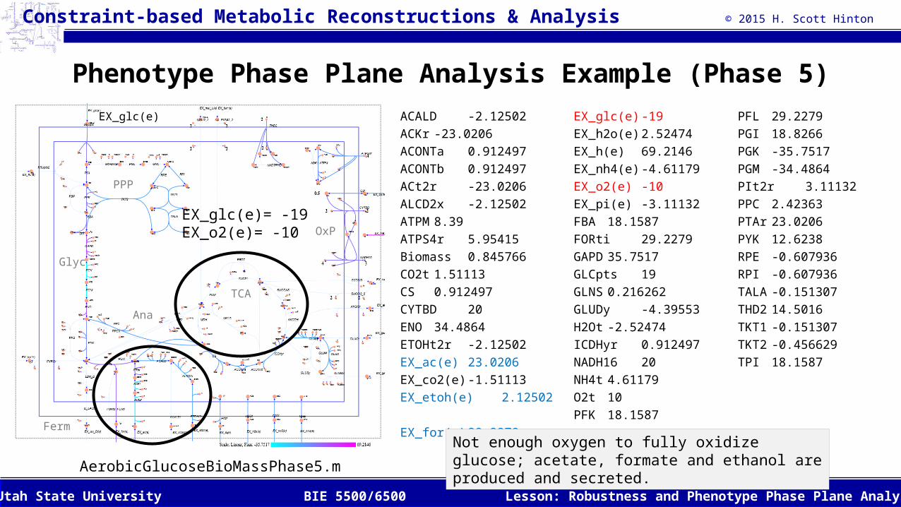
Phenotype Phase Plane Analysis Example (Phase 5)
ACALD -2.12502ACKr -23.0206ACONTa 0.912497ACONTb 0.912497ACt2r -23.0206ALCD2x -2.12502ATPM 8.39ATPS4r 5.95415Biomass 0.845766CO2t 1.51113CS 0.912497CYTBD 20ENO 34.4864ETOHt2r -2.12502EX_ac(e) 23.0206EX_co2(e) -1.51113EX_etoh(e)2.12502EX_for(e) 29.2279
AerobicGlucoseBioMassPhase5.m
EX_glc(e) -19EX_h2o(e) 2.52474EX_h(e) 69.2146EX_nh4(e) -4.61179EX_o2(e) -10EX_pi(e) -3.11132FBA 18.1587FORti 29.2279GAPD 35.7517GLCpts 19GLNS 0.216262GLUDy -4.39553H2Ot -2.52474ICDHyr 0.912497NADH16 20NH4t 4.61179O2t 10PFK 18.1587
PFL 29.2279PGI 18.8266PGK -35.7517PGM -34.4864PIt2r 3.11132PPC 2.42363PTAr 23.0206PYK 12.6238RPE -0.607936RPI -0.607936TALA -0.151307THD2 14.5016TKT1 -0.151307TKT2 -0.456629TPI 18.1587
EX_glc(e)
Ferm
TCA
PPP
Glyc
Ana
OxPEX_glc(e)= -19EX_o2(e)= -10
Not enough oxygen to fully oxidize glucose; acetate, formate and ethanol are produced and secreted.
© 2015 H. Scott Hinton
Lesson: Robustness and Phenotype Phase Plane AnalysisBIE 5500/6500Utah State University
Constraint-based Metabolic Reconstructions & Analysis
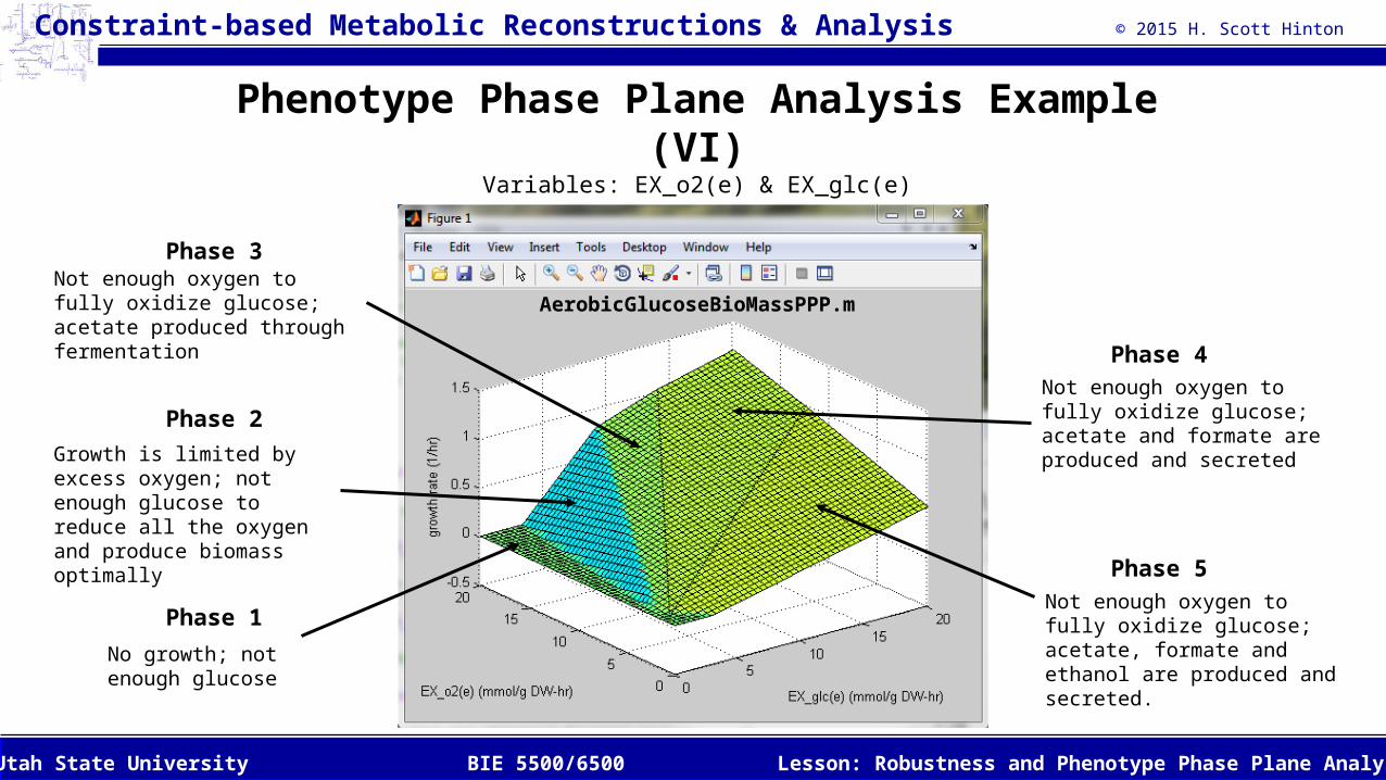
Phenotype Phase Plane Analysis Example (VI)
Variables: EX_o2(e) & EX_glc(e)
Phase 1
Phase 3
Phase 2
Phase 4
Phase 5
No growth; not enough glucose
Growth is limited by excess oxygen; not enough glucose to reduce all the oxygen and produce biomass optimally
Not enough oxygen to fully oxidize glucose; acetate produced through fermentation
Not enough oxygen to fully oxidize glucose; acetate and formate are produced and secreted
Not enough oxygen to fully oxidize glucose; acetate, formate and ethanol are produced and secreted.
AerobicGlucoseBioMassPPP.m
© 2015 H. Scott Hinton
Lesson: Robustness and Phenotype Phase Plane AnalysisBIE 5500/6500Utah State University
Constraint-based Metabolic Reconstructions & Analysis
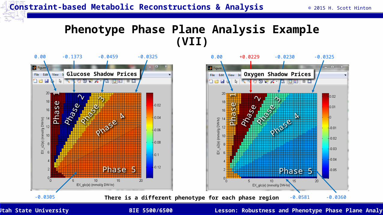
Phenotype Phase Plane Analysis Example (VII)
There is a different phenotype for each phase region
Ph
ase
1Ph
ase
2Ph
ase
3
Phase 4
Phase 5
+0.02290.00 -0.0230 -0.0325
-0.0581 -0.0360
Oxygen Shadow Prices
Ph
ase
1Ph
ase
2Ph
ase
3
Phase 4
Phase 5
-0.13730.00 -0.0459 -0.0325
-0.0305
Glucose Shadow Prices
© 2015 H. Scott Hinton
Lesson: Robustness and Phenotype Phase Plane AnalysisBIE 5500/6500Utah State University
Constraint-based Metabolic Reconstructions & Analysis
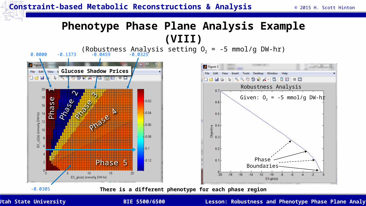
Phenotype Phase Plane Analysis Example (VIII)
(Robustness Analysis setting O2 = -5 mmol/g DW-hr)
There is a different phenotype for each phase region
Given: O2 = -5 mmol/g DW-hr
PhaseBoundaries
Robustness Analysis
Ph
ase
1Ph
ase
2Ph
ase
3
Phase 4
Phase 5
-0.13730.0000 -0.0459 -0.0325
-0.0305
Glucose Shadow Prices
© 2015 H. Scott Hinton
Lesson: Robustness and Phenotype Phase Plane AnalysisBIE 5500/6500Utah State University
Constraint-based Metabolic Reconstructions & Analysis
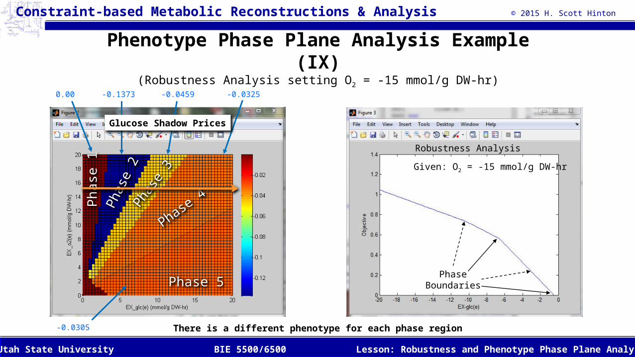
Phenotype Phase Plane Analysis Example (IX)
(Robustness Analysis setting O2 = -15 mmol/g DW-hr)
There is a different phenotype for each phase region
Given: O2 = -15 mmol/g DW-hr
PhaseBoundaries
Robustness Analysis
Ph
ase
1Ph
ase
2Ph
ase
3
Phase 4
Phase 5
-0.13730.00 -0.0459 -0.0325
-0.0305
Glucose Shadow Prices
© 2015 H. Scott Hinton
Lesson: Robustness and Phenotype Phase Plane AnalysisBIE 5500/6500Utah State University
Constraint-based Metabolic Reconstructions & Analysis
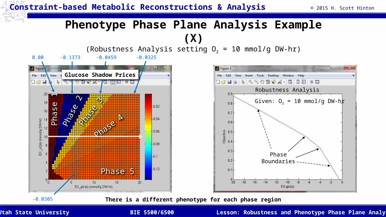
Phenotype Phase Plane Analysis Example (X)
(Robustness Analysis setting O2 = 10 mmol/g DW-hr)
There is a different phenotype for each phase region
Given: O2 = 10 mmol/g DW-hr
PhaseBoundaries
Robustness Analysis
Ph
ase
1Ph
ase
2Ph
ase
3
Phase 4
Phase 5
-0.13730.00 -0.0459 -0.0325
-0.0305
Glucose Shadow Prices
© 2015 H. Scott Hinton
Lesson: Robustness and Phenotype Phase Plane AnalysisBIE 5500/6500Utah State University
Constraint-based Metabolic Reconstructions & Analysis
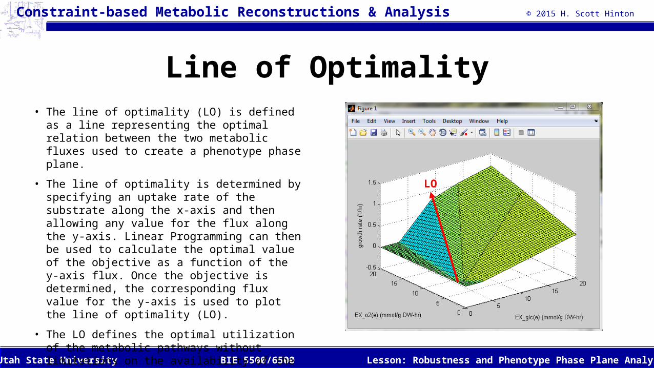
Line of Optimality• The line of optimality (LO) is defined as a line
representing the optimal relation between the two metabolic fluxes used to create a phenotype phase plane.
• The line of optimality is determined by specifying an uptake rate of the substrate along the x-axis and then allowing any value for the flux along the y-axis. Linear Programming can then be used to calculate the optimal value of the objective as a function of the y-axis flux. Once the objective is determined, the corresponding flux value for the y-axis is used to plot the line of optimality (LO).
• The LO defines the optimal utilization of the metabolic pathways without limitations on the availability of the substrates.
LO
© 2015 H. Scott Hinton
Lesson: Robustness and Phenotype Phase Plane AnalysisBIE 5500/6500Utah State University
Constraint-based Metabolic Reconstructions & Analysis
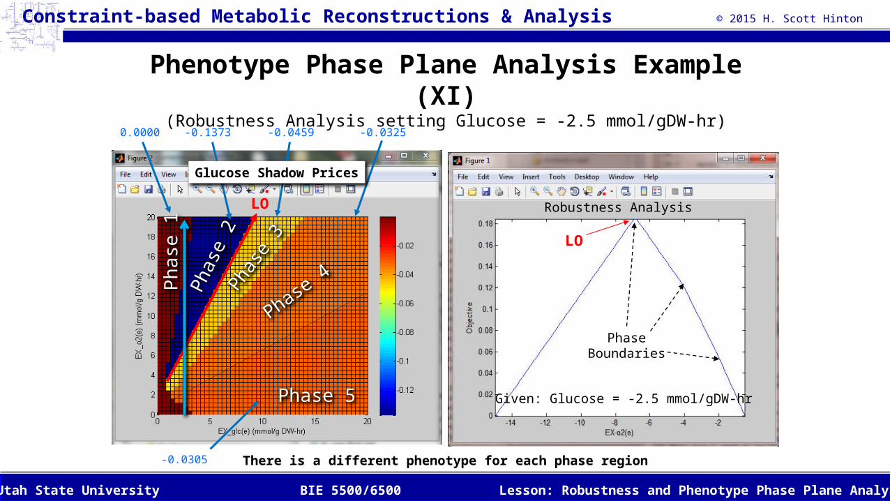
Phenotype Phase Plane Analysis Example (XI)
(Robustness Analysis setting Glucose = -2.5 mmol/gDW-hr)
Ph
ase
1Ph
ase
2Ph
ase
3
Phase 4
Phase 5
-0.13730.0000 -0.0459 -0.0325
-0.0305 There is a different phenotype for each phase region
Given: Glucose = -2.5 mmol/gDW-hr
PhaseBoundaries
Robustness AnalysisLO
LO
Glucose Shadow Prices
© 2015 H. Scott Hinton
Lesson: Robustness and Phenotype Phase Plane AnalysisBIE 5500/6500Utah State University
Constraint-based Metabolic Reconstructions & Analysis
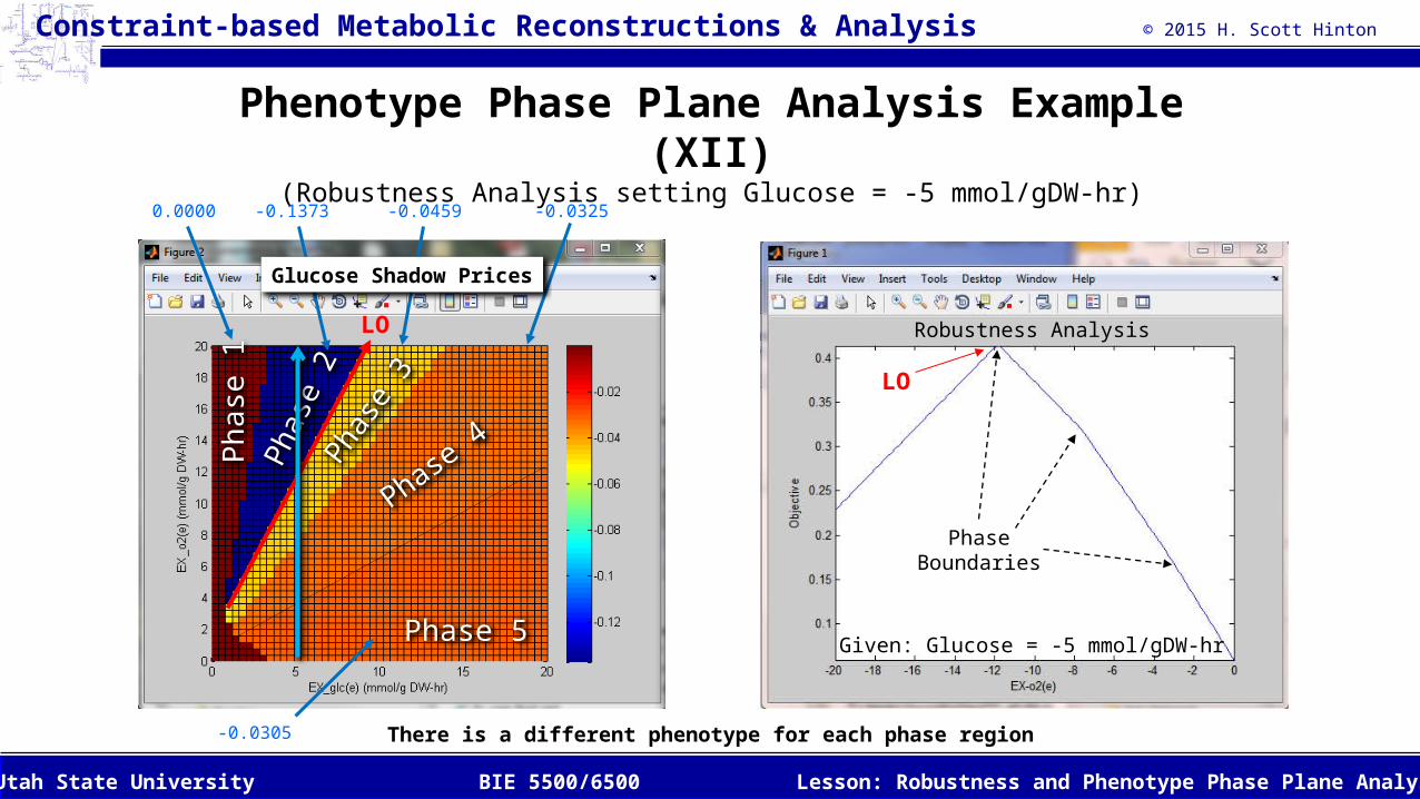
Phenotype Phase Plane Analysis Example (XII)
(Robustness Analysis setting Glucose = -5 mmol/gDW-hr)
There is a different phenotype for each phase region
Given: Glucose = -5 mmol/gDW-hr
PhaseBoundaries
Robustness Analysis
LO
Ph
ase
1Ph
ase
2Ph
ase
3
Phase 4
Phase 5
-0.13730.0000 -0.0459 -0.0325
-0.0305
LO
Glucose Shadow Prices
© 2015 H. Scott Hinton
Lesson: Robustness and Phenotype Phase Plane AnalysisBIE 5500/6500Utah State University
Constraint-based Metabolic Reconstructions & Analysis
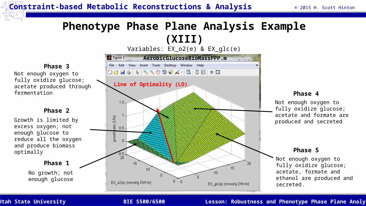
Phenotype Phase Plane Analysis Example (XIII)
Variables: EX_o2(e) & EX_glc(e)
Phase 1
Phase 3
Phase 2
Phase 4
Phase 5
No growth; not enough glucose
Growth is limited by excess oxygen; not enough glucose to reduce all the oxygen and produce biomass optimally
Not enough oxygen to fully oxidize glucose; acetate produced through fermentation
Not enough oxygen to fully oxidize glucose; acetate and formate are produced and secreted
Not enough oxygen to fully oxidize glucose; acetate, formate and ethanol are produced and secreted.
Line of Optimality (LO)
AerobicGlucoseBioMassPPP.m
© 2015 H. Scott Hinton
Lesson: Robustness and Phenotype Phase Plane AnalysisBIE 5500/6500Utah State University
Constraint-based Metabolic Reconstructions & Analysis
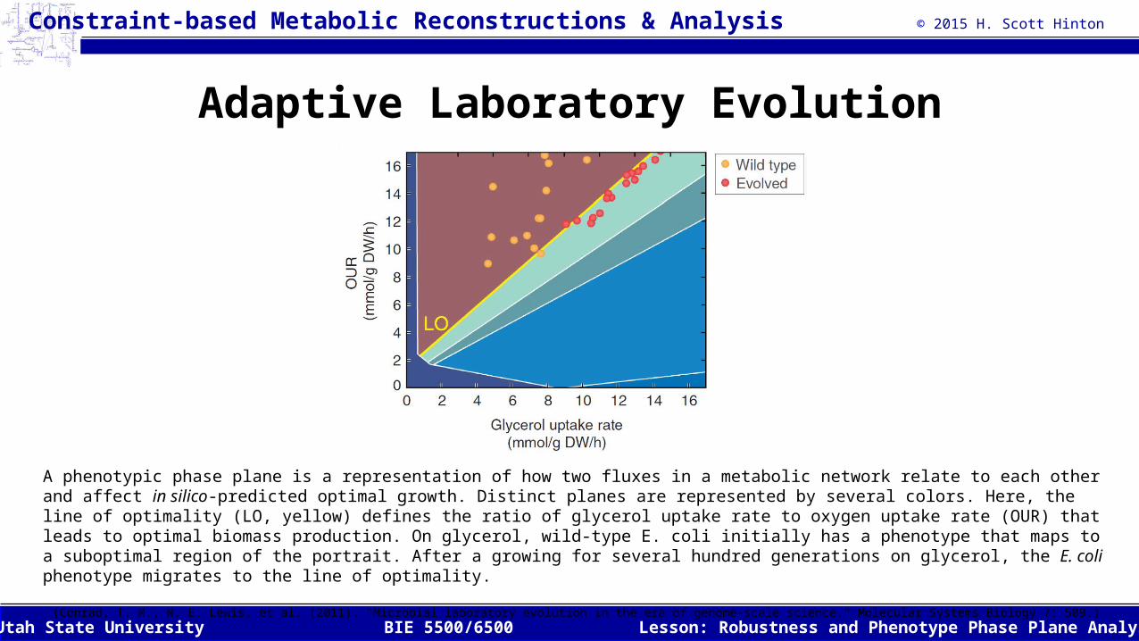
Adaptive Laboratory Evolution
A phenotypic phase plane is a representation of how two fluxes in a metabolic network relate to each other and affect in silico-predicted optimal growth. Distinct planes are represented by several colors. Here, the line of optimality (LO, yellow) defines the ratio of glycerol uptake rate to oxygen uptake rate (OUR) that leads to optimal biomass production. On glycerol, wild-type E. coli initially has a phenotype that maps to a suboptimal region of the portrait. After a growing for several hundred generations on glycerol, the E. coli phenotype migrates to the line of optimality.
(Conrad, T. M., N. E. Lewis, et al. (2011). "Microbial laboratory evolution in the era of genome-scale science." Molecular Systems Biology 7: 509.)
© 2015 H. Scott Hinton
Lesson: Robustness and Phenotype Phase Plane AnalysisBIE 5500/6500Utah State University
Constraint-based Metabolic Reconstructions & Analysis
Lesson Outline
• Robustness Analysis
• Shadow Prices
• Reduced Costs
• Phenotype Phase Plane
Analysis

© 2015 H. Scott Hinton
Lesson: Robustness and Phenotype Phase Plane AnalysisBIE 5500/6500Utah State University
Constraint-based Metabolic Reconstructions & Analysis
Extra Slides
© 2015 H. Scott Hinton
Lesson: Robustness and Phenotype Phase Plane AnalysisBIE 5500/6500Utah State University
Constraint-based Metabolic Reconstructions & Analysis
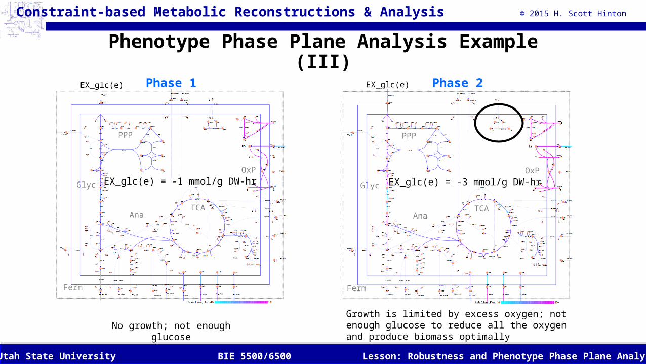
Phenotype Phase Plane Analysis Example (III)
EX_glc(e) = -1 mmol/g DW-hr
Phase 1EX_glc(e)
Ferm
TCA
PPP
Glyc
Ana
OxP
No growth; not enough glucose
EX_glc(e) = -3 mmol/g DW-hr
Phase 2EX_glc(e)
Ferm
TCA
PPP
Glyc
Ana
OxP
Growth is limited by excess oxygen; not enough glucose to reduce all the oxygen and produce biomass optimally
© 2015 H. Scott Hinton
Lesson: Robustness and Phenotype Phase Plane AnalysisBIE 5500/6500Utah State University
Constraint-based Metabolic Reconstructions & Analysis
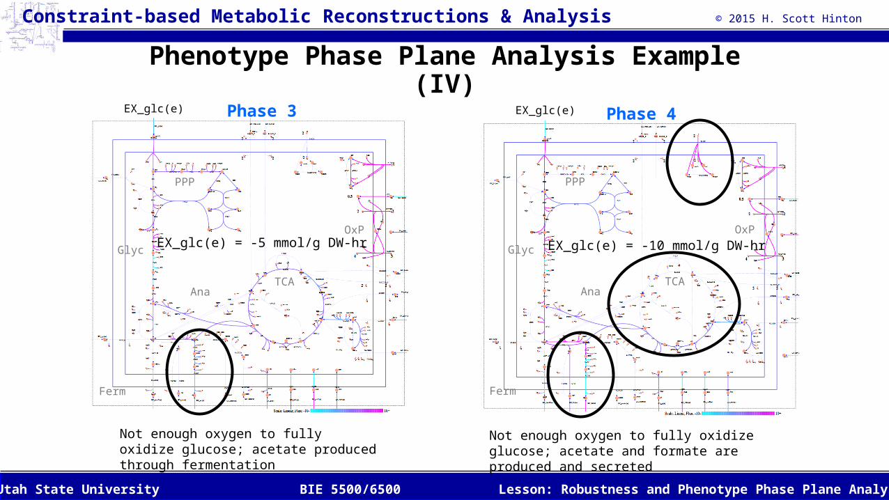
Phenotype Phase Plane Analysis Example (IV)
Phase 3
EX_glc(e) = -5 mmol/g DW-hr
EX_glc(e)
Ferm
TCA
PPP
Glyc
Ana
OxP
Not enough oxygen to fully oxidize glucose; acetate produced through fermentation
Phase 4
EX_glc(e) = -10 mmol/g DW-hr
EX_glc(e)
Ferm
TCA
PPP
Glyc
Ana
OxP
Not enough oxygen to fully oxidize glucose; acetate and formate are produced and secreted
© 2015 H. Scott Hinton
Lesson: Robustness and Phenotype Phase Plane AnalysisBIE 5500/6500Utah State University
Constraint-based Metabolic Reconstructions & Analysis
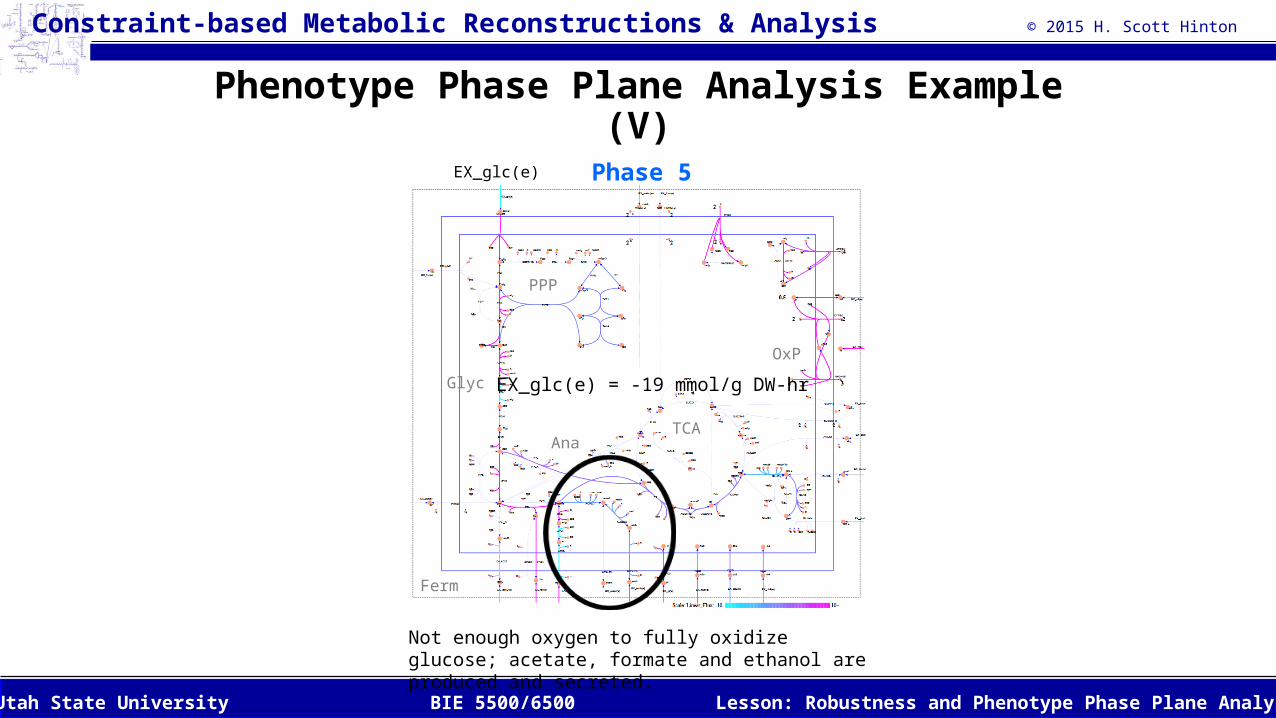
Phenotype Phase Plane Analysis Example (V)
Phase 5
EX_glc(e) = -19 mmol/g DW-hr
EX_glc(e)
Ferm
TCA
PPP
Glyc
Ana
OxP
Not enough oxygen to fully oxidize glucose; acetate, formate and ethanol are produced and secreted.