Embed Size (px)
Citation preview
IMPLEMENTING AND ANALYZING ONLINE EXPERIMENTSSEAN J. TAYLOR 28 JUL 2015 MULTITHREADED DATA

WHO AM I?
• Core Data Science Team at Facebook
• PhD from NYU in Information Systems
• Four academic papers employing online field experiments
• Teach and consult on experimental design at Facebook
http://seanjtaylor.comhttp://github.com/seanjtaylorhttp://facebook.com/seanjtaylor@seanjtaylor
I ASSUME YOU KNOW
• Why causality matters
• A little bit of Python and R
• Basic statistics + linear regression

SIMPLEST POSSIBLE EXPERIMENT
user_id version spent
123 B $10
596 A $0
456 A $4
991 B $9
def get_version(user_id): if user_id % 2: return 'A' else: return 'B'
> t.test(c(0, 4), c(10, 9))
Welch Two Sample t-‐test
data: c(0, 4) and c(10, 9) t = -‐3.638, df = 1.1245, p-‐value = 0.1487 alternative hypothesis: true difference in means is not equal to 0 95 percent confidence interval: -‐27.74338 12.74338 sample estimates: mean of x mean of y 2.0 9.5

FIN
COMMON PROBLEMS
• Type I errors from measuring too many effects
• Type II and M errors from lack of power
• Repeated use of the same population (“pollution”)
• Type I errors from violation of the i.i.d. assumption
• Composing many changes into one experiment
POWEROR
THE ONLY WAY TO TRULY FAIL AT AN EXPERIMENT
OR
THE SIZE OF YOUR CONFIDENCE INTERVALS
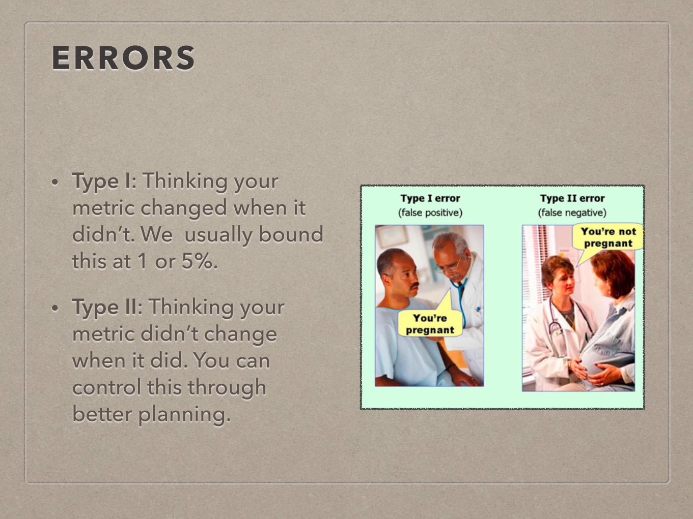
ERRORS
• Type I: Thinking your metric changed when it didn’t. We usually bound this at 1 or 5%.
• Type II: Thinking your metric didn’t change when it did. You can control this through better planning.
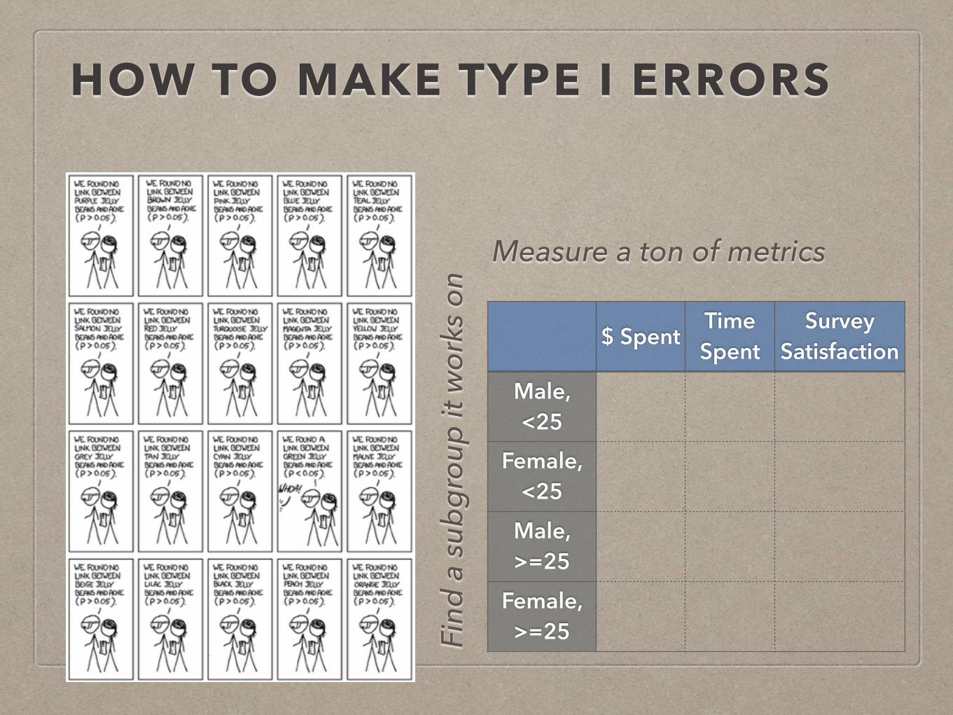
HOW TO MAKE TYPE I ERRORS
$ SpentTime Spent
Survey Satisfaction
oMale, <25
Female, <25
Male, >=25
Female, >=25
Measure a ton of metrics
Find
a su
bgro
up it
wor
ks o
n
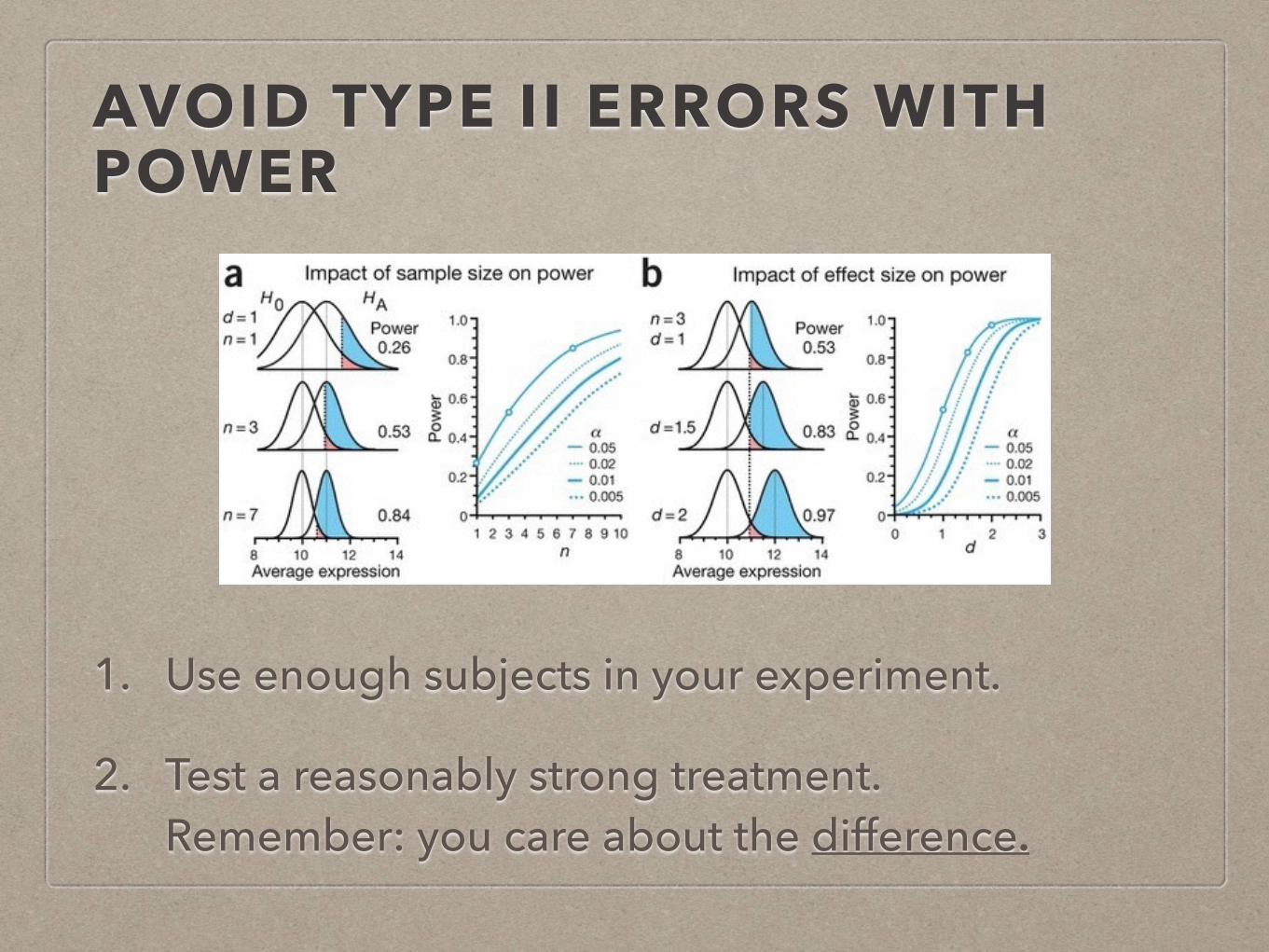
AVOID TYPE II ERRORS WITH POWER
1. Use enough subjects in your experiment.
2. Test a reasonably strong treatment. Remember: you care about the difference.

POWER ANALYSIS
First step in designing an experiment is to determine how much data you’ll need to learn the answer to your question.
Process:
• set the smallest effect size you’d like to detect.
• simulate your experiment 200 times at various sample sizes
• count the number of simulated experiments where you correctly reject the null of effect=0.

TYPE M ERRORS
• Magnitude error: reporting an effect size which is too large
• happens when your experiment is underpowered AND you only report the significant results

IMPLEMENTATION
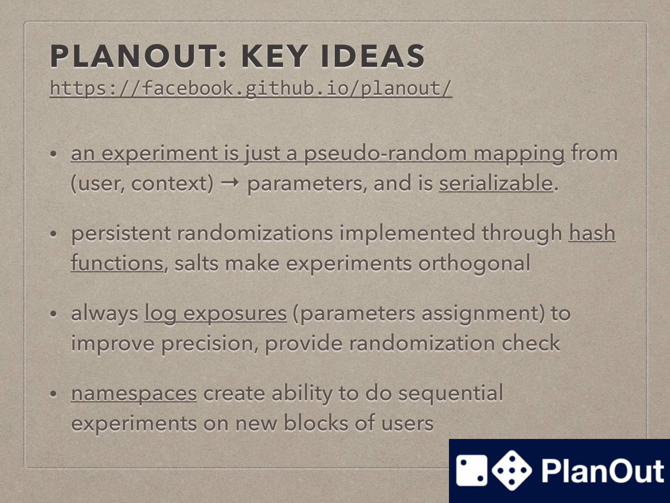
PLANOUT: KEY IDEAS
• an experiment is just a pseudo-random mapping from (user, context) → parameters, and is serializable.
• persistent randomizations implemented through hash functions, salts make experiments orthogonal
• always log exposures (parameters assignment) to improve precision, provide randomization check
• namespaces create ability to do sequential experiments on new blocks of users
https://facebook.github.io/planout/

A/B TESTING IN PLANOUTfrom planout.ops.random import * from planout.experiment import SimpleExperiment
class ButtonCopyExperiment(SimpleExperiment): def assign(self, params, user_id): # `params` is always the first argument. params.button_text = UniformChoice( choices=["Buy now!", "Buy later!"], unit=user_id )
# Later in your production code: from myexperiments import ButtonCopyExperiment
e = ButtonCopyExperiment(user_id=212) print(e.get('button_text'))
# Event later: e = ButtonCopyExperiment(user_id=212) e.log_event('purchase', {'amount': 9.43})

PLANOUT LOGS → DATA
{"inputs": {"user_id": 212}, "name": "ButtonCopyExperiment", "checksum": "646e69a5", "params": {"button_text": "Buy later!"}, "time": 1437952369, "salt": "ButtonCopyExperiment", "event": “exposure"}
{"inputs": {"user_id": 212}, "name": "ButtonCopyExperiment", "checksum": "646e69a5", "params": {"button_text": "Buy later!"}, "time": 1437952369, "extra_data": {"amount": 9.43}, "salt": "ButtonCopyExperiment", "event": "purchase"}
user_id button_text
123 Buy later!
596 Buy later!
456 Buy now!
991 Buy later!
user_id amount
123 $12
596 $9
Exposures
Purchases

ADVANCED DESIGN 1: FACTORIAL DESIGN
• Can use conditional logic as well as other random assignment operators: RandomInteger, RandomFloat, WeightedChoice, Sample.
class FactorialExperiment(SimpleExperiment): def assign(self, params, user_id): params.button_text = UniformChoice( choices=["Buy now!", "Buy later!"], unit=user_id ) params.button_color = UniformChoice( choices=["blue", "orange"], unit=user_id )

ADVANCED DESIGN 2: INCREMENTAL CHANGES
## We're going to try two different button redesigns. class FirstExperiment(SimpleExperiment): def assign(self, params, user_id): # ... set some params
class SecondExperiment(SimpleExperiment): def assign(self, params, user_id): # ... set some params differently class ButtonNamespace(SimpleNamespace): def setup(self): self.name = 'button_experiment_sequence' self.primary_unit = 'user_id' self.num_segments = 1000
def setup_experiments(): # allocate and deallocate experiments here # First gets 100 out of 1000 segments. self.add_experiment('first', FirstExperiment, 100) self.add_experiment('second', SecondExperiment, 100)

ADVANCED DESIGN 3: WITHIN-SUBJECTS
Previous experiments persistently assigned same treatment to user, but unit of analysis can be more complex:
class DiscountExperiment(SimpleExperiment): def assign(self, params, user_id, item_id): params.discount = BernoulliTrial(p=0.1, unit=[user_id, item_id]) if params.discount: params.discount_amount = RandomInteger( min=5, max=15, unit=user_id ) else: params.discount_amount = 0
e = DiscountExperiment(user_id=212, item_id=2) print(e.get('discount_amount'))

ANALYSIS

THE IDEAL DATA SET
Subject / User
Gender Age Button Size
Button Text
Spent Bounce
Erin F 22 Large Buy Now!
$20 0
Ashley F 29 Large Buy Later!
$4 0
Gary M 34 Small Buy Now!
$0 1
Leo M 18 Large Buy Now!
$0 1
Ed M 46 Small Buy Later!
$9 0
Sam M 25 Small Buy Now!
$5 0
Independent Observations
Randomly Assigned MetricsPre-experiment
Covariates{ { {
{

SIMPLEST CASE: OLS
> summary(lm(spent ~ button.size, data = df))
Call: lm(formula = spent ~ button.size, data = df)
Residuals: 1 2 3 4 5 6 10.0 -‐0.5 -‐4.5 -‐10.0 4.5 0.5
Coefficients: Estimate Std. Error t value Pr(>|t|) (Intercept) 10.000 5.489 1.822 0.143 factor(button.size)s -‐5.500 6.722 -‐0.818 0.459
Residual standard error: 7.762 on 4 degrees of freedom Multiple R-‐squared: 0.1434, Adjusted R-‐squared: -‐0.07079 F-‐statistic: 0.6694 on 1 and 4 DF, p-‐value: 0.4592

DATA REDUCTION
Subject Xi Di Yi
Evan M 0 1
Ashley F 0 1
Greg M 1 0
Leena F 1 0
Ema F 0 0
Seamus M 1 1
X D Y Cases
M 0 1 1
M 1 1 1
F 0 1 1
F 1 1 0
M 0 0 0
M 1 0 1
F 0 0 1
F 1 0 1
N # treatments X # groups X #outcomes
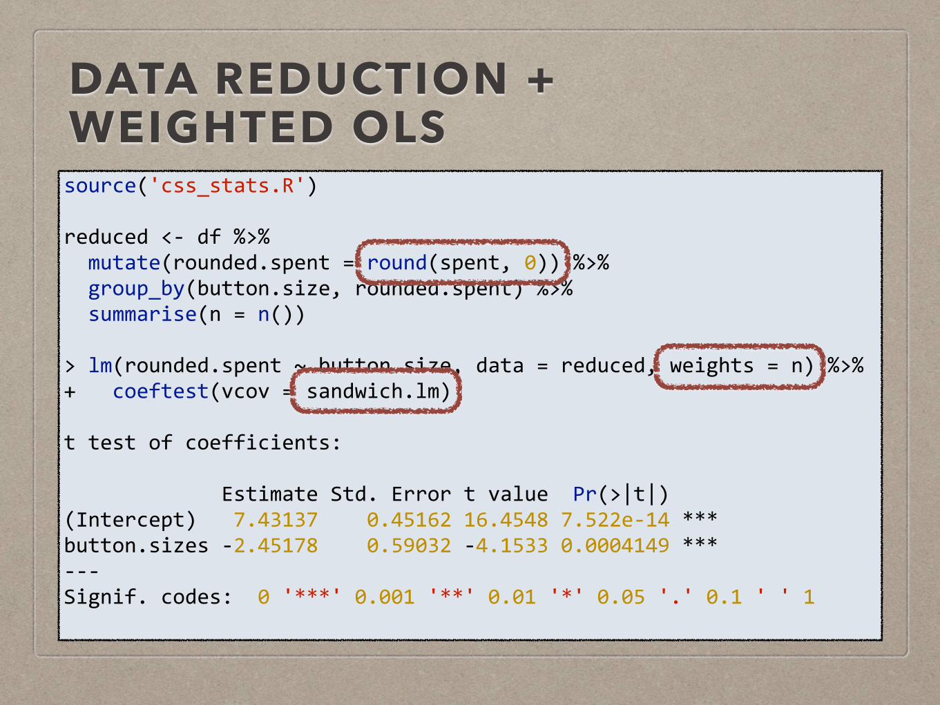
source('css_stats.R')
reduced <-‐ df %>% mutate(rounded.spent = round(spent, 0)) %>% group_by(button.size, rounded.spent) %>% summarise(n = n())
> lm(rounded.spent ~ button.size, data = reduced, weights = n) %>% + coeftest(vcov = sandwich.lm)
t test of coefficients:
Estimate Std. Error t value Pr(>|t|) (Intercept) 7.43137 0.45162 16.4548 7.522e-‐14 *** button.sizes -‐2.45178 0.59032 -‐4.1533 0.0004149 *** -‐-‐-‐ Signif. codes: 0 '***' 0.001 '**' 0.01 '*' 0.05 '.' 0.1 ' ' 1
DATA REDUCTION + WEIGHTED OLS

FACTORIAL DESIGNS
• Identify two types of effects: marginal and interactions. Need to fix one group as the baseline.
> coeftest(lm(spent ~ button.size * button.text, data = df))
t test of coefficients:
Estimate Std. Error t value Pr(>|t|) (Intercept) 6.79643 0.62998 10.7884 < 2.2e-‐16 *** button.sizes -‐2.43253 0.86673 -‐2.8066 0.006064 ** button.textn 2.11611 0.86673 2.4415 0.016458 * button.sizes:button.textn -‐2.57660 1.27584 -‐2.0195 0.046219 * -‐-‐-‐ Signif. codes: 0 '***' 0.001 '**' 0.01 '*' 0.05 '.' 0.1 ' ' 1

USING COVARIATES TO GAIN PRECISION
• With simple random assignment, using covariates is not necessary.
• However, you can improve precision of ATE estimates if covariates explain a lot of variation in the potential outcomes.
• Can be added to a linear model and SEs should get smaller if they are helpful.

NON-IID DATA
• Repeated observations of the same user are not independent.
• Ditto if you ‘re experimenting on certain items only.
• If you ignore dependent data, the true confidence intervals are larger than you think.
Subject / User
Item Button Size
Spent
Erin Shirt Large $20
Erin Socks Large $4
Erin Pants Large $0
Leo Shirt Large $0
Ed Shirt Small $9
Ed Socks Small $5
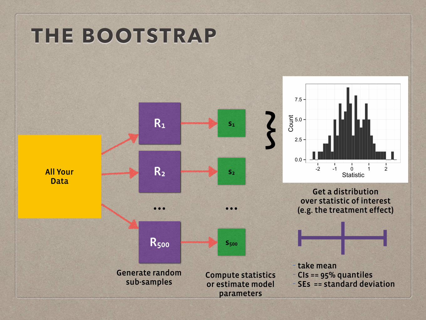
THE BOOTSTRAP
R1
All Your Data
R2
…
R500
Generate random sub-samples
s1
s2
s500
Compute statistics or estimate model
parameters
…
}0.0
2.5
5.0
7.5
-2 -1 0 1 2Statistic
Count
Get a distribution over statistic of interest
(e.g. the treatment effect)
- take mean - CIs == 95% quantiles - SEs == standard deviation
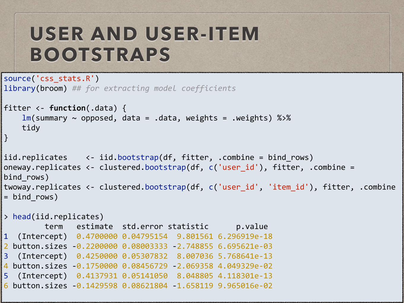
USER AND USER-ITEM BOOTSTRAPS
source('css_stats.R') library(broom) ## for extracting model coefficients
fitter <-‐ function(.data) { lm(summary ~ opposed, data = .data, weights = .weights) %>% tidy }
iid.replicates <-‐ iid.bootstrap(df, fitter, .combine = bind_rows) oneway.replicates <-‐ clustered.bootstrap(df, c('user_id'), fitter, .combine = bind_rows) twoway.replicates <-‐ clustered.bootstrap(df, c('user_id', 'item_id'), fitter, .combine = bind_rows)
> head(iid.replicates) term estimate std.error statistic p.value 1 (Intercept) 0.4700000 0.04795154 9.801561 6.296919e-‐18 2 button.sizes -‐0.2200000 0.08003333 -‐2.748855 6.695621e-‐03 3 (Intercept) 0.4250000 0.05307832 8.007036 5.768641e-‐13 4 button.sizes -‐0.1750000 0.08456729 -‐2.069358 4.049329e-‐02 5 (Intercept) 0.4137931 0.05141050 8.048805 4.118301e-‐13 6 button.sizes -‐0.1429598 0.08621804 -‐1.658119 9.965016e-‐02
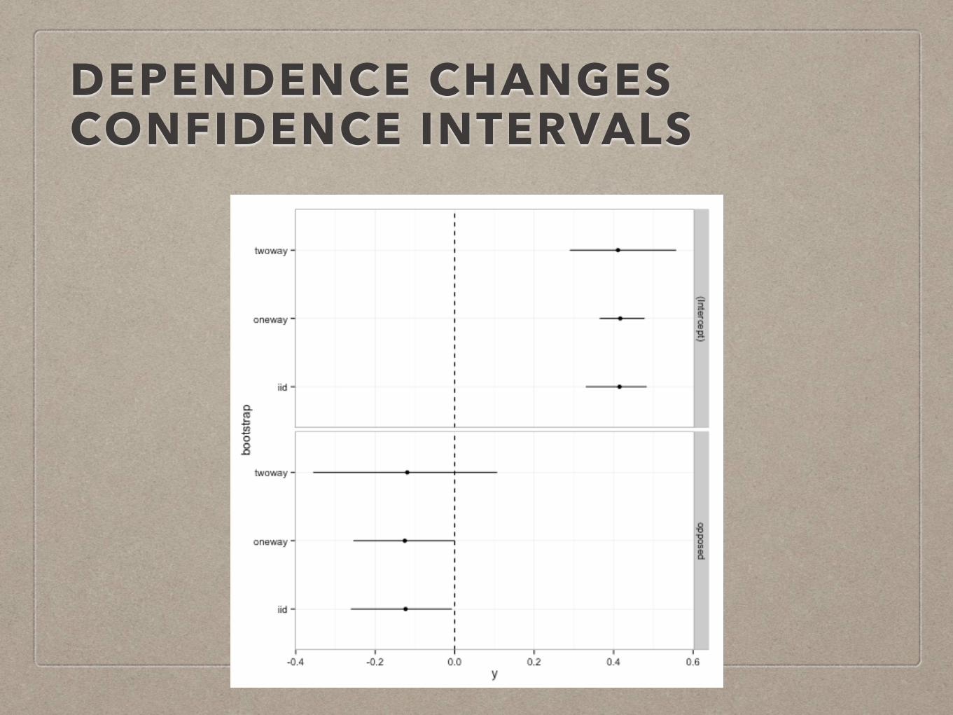
DEPENDENCE CHANGES CONFIDENCE INTERVALS

DATA REDUCTION WITH DEPENDENT DATA
Subject Di Yij
Evan 1 1
Evan 1 0
Ashley 0 1
Ashley 0 1
Ashley 0 1
Greg 1 0
Leena 1 0
Leena 1 1
Ema 0 0
Seamus 1 1
Create bootstrap replicates
R1
R2
R3
reduce the replicates as if they’re i.i.d.
r1
r2
r3
s1
s2
s3
compute statistics on reduced data
THANKS! HERE ARE SOME RESOURCES:
• Me: http://seanjtaylor.com
• These slides:http://www.slideshare.net/seanjtaylor/implementing-and-analyzing-online-experiments
• Full Featured Tutorial: http://eytan.github.io/www-15-tutorial/
• “Field Experiments” by Gerber and Green