The 15th Scandinavian International Conference on Fluid Power, SICFP’17, June 7-9, 2017, Linköping, Sweden

Towards Finding the Optimal Bucket Filling Strategy through Simulation

R. Filla1 and B. Frank1,2

1Volvo Construction Equipment, Emerging Technologies, 631 85 Eskilstuna, Sweden 2Lund University, Faculty of Engineering, 221 00 Lund, Sweden

E-mail: reno.filla@volvo.com, bobbie.frank@volvo.com

Abstract The purpose of earth-moving equipment like wheel loaders is to engage with the ground or other material. It is therefore obvious that the bucket filling phase must be included when studying optimal machine control over a complete working cycle because total productivity and efficiency of the machine are to a large extent determined by it. This paper reports and discusses the results of research into how to utilize Discrete Element Method simulations in combination with Optimal Control to find the optimal bucket filling strategy and what has been learned regarding preparing and conducting both simulations of bucket filling and physical testing for verification. This paper also discloses which bucket filling strategy appears to be optimal, based on the results so far – and why we cannot be completely certain.

Keywords: wheel loaders, bucket filling, working cycle, trajectory, optimization, simulation, optimal control, dynamic programming, tool/ground interaction, discrete-element method

1 Introduction Construction machines can be made – and need to be – significantly more energy efficient. Industry knowledge and published research, including our own, indicate that large improvements can be achieved by approaching this task holistically. Construction machinery OEMs will have to make their journey towards significantly increased energy efficiency with these four milestones in mind:

‒ Understanding the machine as one system ‒ Understanding the interaction between machine,

operator and working environment ‒ Understanding the cooperation between several

machines and their operators ‒ Understanding the connection to regional, national

and international transport and energy systems

All these milestones have been previously described in [1]. The topic of this paper relates to milestones 1 and 2 as our research is anchored in the realization that in a working machine like a wheel loader all major systems interact frequently, all phases in a working cycle are connected, and both operator and working environment play a decisive role when it comes to productivity and energy efficiency of the total system.

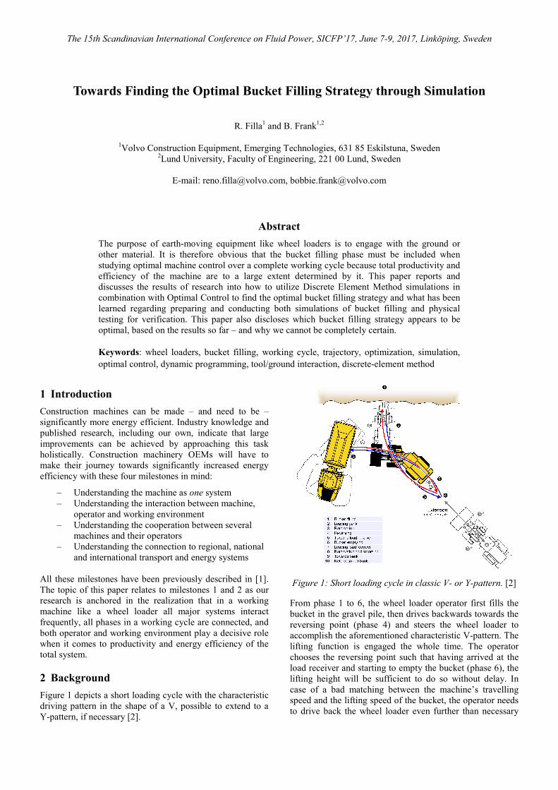
2 Background Figure 1 depicts a short loading cycle with the characteristic driving pattern in the shape of a V, possible to extend to a Y-pattern, if necessary [2].

Figure 1: Short loading cycle in classic V- or Y-pattern. [2]

From phase 1 to 6, the wheel loader operator first fills the bucket in the gravel pile, then drives backwards towards the reversing point (phase 4) and steers the wheel loader to accomplish the aforementioned characteristic V-pattern. The lifting function is engaged the whole time. The operator chooses the reversing point such that having arrived at the load receiver and starting to empty the bucket (phase 6), the lifting height will be sufficient to do so without delay. In case of a bad matching between the machine’s travelling speed and the lifting speed of the bucket, the operator needs to drive back the wheel loader even further than necessary

for maneuvering alone. This additional leg transforms the V-pattern into a Y.

In previous research [3][4] it has been examined whether the driving pattern necessarily has to resemble a V or Y as it appears that this pattern has emerged from the operators’ desire to minimize the personal workload, rather than maximize energy efficiency, for a required productivity. The traditional cycle in Figure 1 might not necessarily be the most productive or the most energy-efficient way for new non-conventional systems like hybrids or autonomous machines where the operator’s requirements are less dominant or taken out of the loop completely. However, papers [3][4] showed that the classic V- or Y-cycle is a good and robust choice and seems to be recommendable for virtually all situations where such driving pattern is not prevented by the layout of the site.

Based on this conclusion research has then been focused on how to optimally control the actuators of a wheel loader for maximum energy efficiency [5], basically covering phases 2 to 10 in Figure 1 with an assumed attachment position in the beginning. However, this exclusion of the bucket filling phase is a serious simplification because how the bucket is filled in phase 1 and at what height the bucket is retracted from the pile has a significant influence on the overall energy efficiency of a wheel loader in a short loading cycle [2][6].

We have therefore used DEM (Discrete Element Method) particle simulation to study how bucket filling can be simulated in detail [2]. In order to avoid slowing down simulation of loading cycle phases 2 to 6 a non-coupled approach was chosen for the bucket filling in phase 1, which means that the bucket was considered in isolation, moving along a (large) set of pre-defined trajectories.

As discussed at length in [7] this approach has the obvious flaw that the tight coupling of forces leading to a complex interaction of the machine’s subsystems (engine, drivetrain, hydraulics etc.), the work environment and the operator is largely disregarded. Even though the loader’s linkage has been represented through the way the trajectories have been generated [2] and/or how the simulation results have been analyzed [7], this limited approach falls short of the full simulation scope actually required. The overall cycle efficiency value and thus the performance of a particular bucket filling strategy are first apparent after the wheel loader has arrived at the load receiver to empty the bucket. Therefore the simulation must comprise a complete machine model operated by an adaptable operator model in a full working cycle, executed in a comprehensive model of the work place – and run in an overall optimization loop of the bucket trajectory. However, this is not feasible today and must remain a vision for the moment being.

We have thus been left with the pragmatic approach of isolating the bucket and prescribing its nominal motion independent of any resistive forces that might interfere with the actual control. Papers [1][2] have discussed the setup and results of these simulations and [1] has also shown a simplistic way of how the evaluate them in the context of a complete loading cycle.

The next step for reaching the vision of the comprehensive, integrated optimization described above has been Optimal Control of machine actuators in all phases of a prescribed loading cycle, using Dynamic Programming, which paper [7] reports. The machine studied is the electric series hybrid wheel loader briefly discussed in [8][9], which has been the precursor and foundation of the “LX1” concept loader [10].

In the paper at hand we will revisit the bucket filling in both simulation and practice, discuss how to prepare and conduct testing virtually and physically, and provide a self-critical assessment of the results achieved.

3 Simulation

3.1 Process

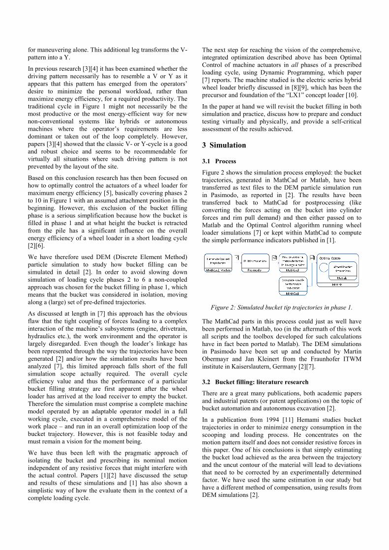
Figure 2 shows the simulation process employed: the bucket trajectories, generated in MathCad or Matlab, have been transferred as text files to the DEM particle simulation run in Pasimodo, as reported in [2]. The results have been transferred back to MathCad for postprocessing (like converting the forces acting on the bucket into cylinder forces and rim pull demand) and then either passed on to Matlab and the Optimal Control algorithm running wheel loader simulations [7] or kept within MathCad to compute the simple performance indicators published in [1].

Figure 2: Simulated bucket tip trajectories in phase 1.

The MathCad parts in this process could just as well have been performed in Matlab, too (in the aftermath of this work all scripts and the toolbox developed for such calculations have in fact been ported to Matlab). The DEM simulations in Pasimodo have been set up and conducted by Martin Obermayr and Jan Kleinert from the Fraunhofer ITWM institute in Kaiserslautern, Germany [2][7].

3.2 Bucket filling: literature research

There are a great many publications, both academic papers and industrial patents (or patent applications) on the topic of bucket automation and autonomous excavation [2].

In a publication from 1994 [11] Hemami studies bucket trajectories in order to minimize energy consumption in the scooping and loading process. He concentrates on the motion pattern itself and does not consider resistive forces in this paper. One of his conclusions is that simply estimating the bucket load achieved as the area between the trajectory and the uncut contour of the material will lead to deviations that need to be corrected by an experimentally determined factor. We have used the same estimation in our study but have a different method of compensation, using results from DEM simulations [2].

3.3 Trajectory generation: overview

Ideally the DEM simulation would be part of the overall simulation that includes the Optimal Control scheme. That way both physicality and optimality (local or global, depending on the method chosen) would be ensured. However, no traditional Optimal Control algorithm can be used as the overall problem is not and cannot be made convex to find gradients for optimization. Instead we used an own algorithm based on Dynamic Programming [7]. However, running one big simulation with a complex machine model in a sufficiently detailed environment, controlled by an adaptive operator model is impossible with the calculation resources typically available, because the computational costs using Dynamic Programming would be extraordinary high (though this can change in the near future, considering cloud computing).

Instead, we disconnected the DEM bucket filling simulation from the machine simulation [1][2] by generating a total of 5781 bucket motion trajectories a priori which were then simulated in parallel on a computer cluster of 800 cores for a week. The results of these simulations have then been incorporated into the machine simulation [7].

We have developed four different principle trajectories along which the bucket is moved in DEM simulations. Each trajectory type is the result of interviews with experienced wheel loader operators and represents a different bucket filling strategy commonly employed.

In addition to the desired bucket fill factor (i.e. load mass in the bucket in relation to the nominal load) most trajectories types offer at least one parameter to vary the individual shape. The bucket trajectories are generated a priori using a kinematic model of the wheel loader’s front body, complete with linkage, hydraulic cylinders, bucket, and front axle. Controlling the bucket motion indirectly through cylinder displacements and a longitudinal motion of the machine ensures that only valid bucket positions are prescribed, corresponding to a valid state of the wheel loader’s linkage.

In addition to these four parametric trajectories a fifth set of bucket motions has been generated as an exploration of “all possible” ways for a bucket to move through a pile and end up with the desired fill factor. In this type of trajectory we only considered the bucket motion, initially without taking linkage constraints into account. Bucket positions that do not correspond to a valid state of the wheel loader’s linkage have been filtered out afterwards.

The major simplification with both approaches is that only the nominal motion of the bucket is prescribed, independent of any resistive forces that might interfere with the actual control and without the adaptive behavior of a human operator. This lack of feedback is a significant limitation, but the study gives some meaningful answers, nonetheless. There are clearly also challenges, which will be discussed later.

3.4 Type A: “Slicing cheese”

This type is a literal implementation of the bucket filling strategy advocated by professional machine instructors who

were interviewed prior to our study. Their advice was to move the bucket such as if carving a slice of constant thickness off the material pile.

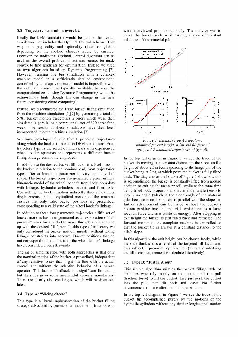
Figure 3: Example type A trajectory, optimized for exit height at 2m and fill factor 1 (grey: all 9 simulated trajectories of type A).

In the top left diagram in Figure 3 we see the trace of the bucket tip moving at a constant distance to the slope until a height of about 2.5m (corresponding to the hinge pin of the bucket being at 2m), at which point the bucket is fully tilted back. The diagrams at the bottom of Figure 3 show how this is accomplished: the bucket is constantly lifted from ground position to exit height (set a priori), while at the same time being tilted back proportionally from initial angle (zero) to maximum angle (which is the slope angle of the material pile, because once the bucket is parallel with the slope, no further advancement can be made without the bucket’s bottom pushing into the material, which creates a large reaction force and is a waste of energy). After stopping at exit height the bucket is just tilted back and retracted. The forward motion of the complete machine is controlled so that the bucket tip is always at a constant distance to the pile’s slope.

In this algorithm the exit height can be chosen freely, while the slice thickness is a result of the targeted fill factor and thus subject to parameter optimization (the value satisfying the fill factor requirement is calculated iteratively).

3.5 Type B: “Just in & out”

This simple algorithm mimics the bucket filling style of operators who rely mostly on momentum and rim pull (traction force) to fill the bucket: they just push the bucket into the pile, then tilt back and leave. No further advancement is made after the initial penetration.

In the top left diagram in Figure 4 we see the trace of the bucket tip accomplished purely by the motions of the hydraulic cylinders without any further longitudinal motion

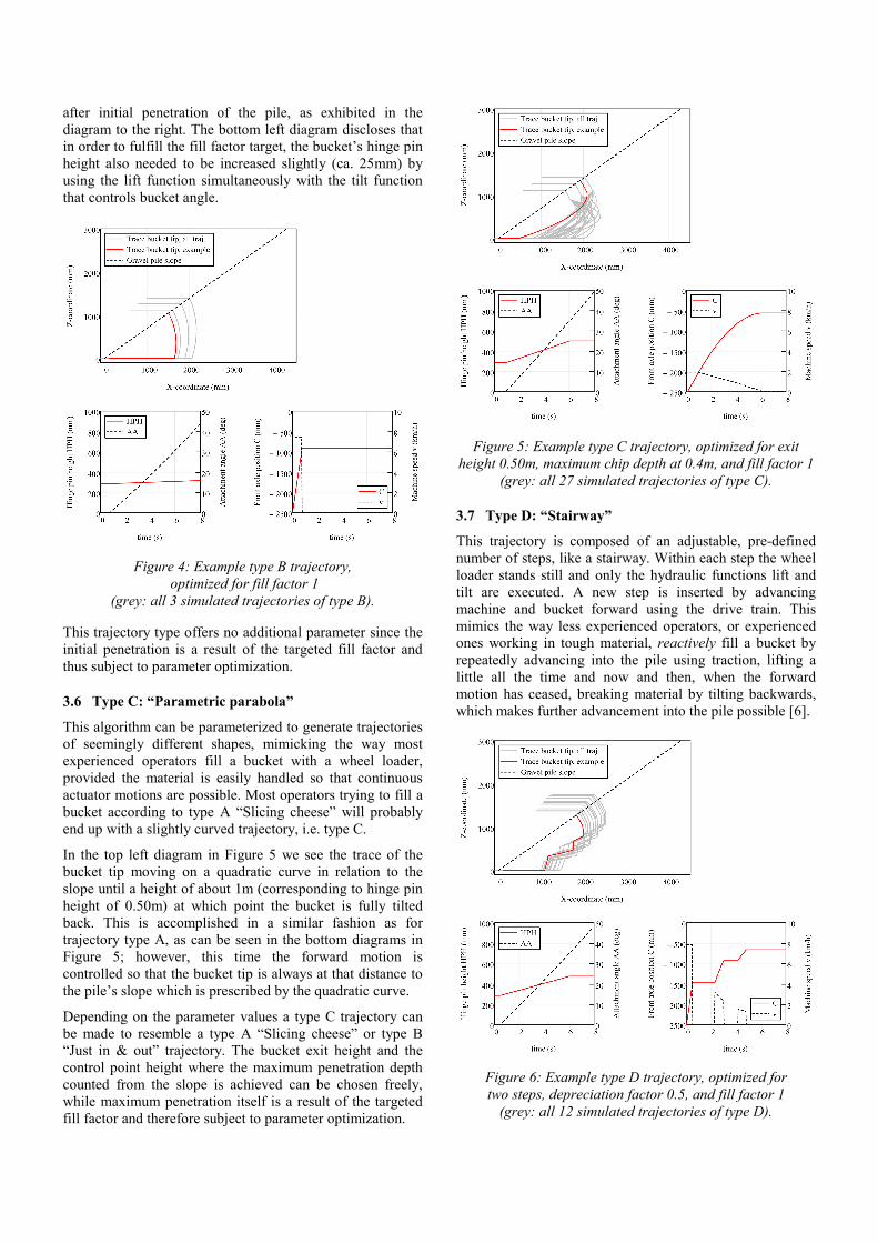
after initial penetration of the pile, as exhibited in the diagram to the right. The bottom left diagram discloses that in order to fulfill the fill factor target, the bucket’s hinge pin height also needed to be increased slightly (ca. 25mm) by using the lift function simultaneously with the tilt function that controls bucket angle.

Figure 4: Example type B trajectory, optimized for fill factor 1

(grey: all 3 simulated trajectories of type B).

This trajectory type offers no additional parameter since the initial penetration is a result of the targeted fill factor and thus subject to parameter optimization.

3.6 Type C: “Parametric parabola”

This algorithm can be parameterized to generate trajectories of seemingly different shapes, mimicking the way most experienced operators fill a bucket with a wheel loader, provided the material is easily handled so that continuous actuator motions are possible. Most operators trying to fill a bucket according to type A “Slicing cheese” will probably end up with a slightly curved trajectory, i.e. type C.

In the top left diagram in Figure 5 we see the trace of the bucket tip moving on a quadratic curve in relation to the slope until a height of about 1m (corresponding to hinge pin height of 0.50m) at which point the bucket is fully tilted back. This is accomplished in a similar fashion as for trajectory type A, as can be seen in the bottom diagrams in Figure 5; however, this time the forward motion is controlled so that the bucket tip is always at that distance to the pile’s slope which is prescribed by the quadratic curve.

Depending on the parameter values a type C trajectory can be made to resemble a type A “Slicing cheese” or type B “Just in & out” trajectory. The bucket exit height and the control point height where the maximum penetration depth counted from the slope is achieved can be chosen freely, while maximum penetration itself is a result of the targeted fill factor and therefore subject to parameter optimization.

Figure 5: Example type C trajectory, optimized for exit height 0.50m, maximum chip depth at 0.4m, and fill factor 1

(grey: all 27 simulated trajectories of type C).

3.7 Type D: “Stairway”

This trajectory is composed of an adjustable, pre-defined number of steps, like a stairway. Within each step the wheel loader stands still and only the hydraulic functions lift and tilt are executed. A new step is inserted by advancing machine and bucket forward using the drive train. This mimics the way less experienced operators, or experienced ones working in tough material, reactively fill a bucket by repeatedly advancing into the pile using traction, lifting a little all the time and now and then, when the forward motion has ceased, breaking material by tilting backwards, which makes further advancement into the pile possible [6].

Figure 6: Example type D trajectory, optimized for two steps, depreciation factor 0.5, and fill factor 1

(grey: all 12 simulated trajectories of type D).

In the top left diagram in Figure 6 we see an example stairway consisting of two stairs after initial penetration. In between the steps the bucket is constantly lifted and tilted. During forward advancement the bucket height and angle also need to be controlled in order to avoid pressing the bucket’s bottom against the cut surface of the gravel pile. At the end of the sequence the bucket is tilted back fully and then retracted.

In this algorithm the number of stairs can be chosen freely, together with a depreciation factor that controls the subsequent advancements in relation to the initial penetration (a depreciation of 0.5 means that the depth of each subsequent penetration is only half as deep as the previous one). The initial penetration depth is a result of the targeted fill factor and therefore derived through parameter optimization by means of iterations.

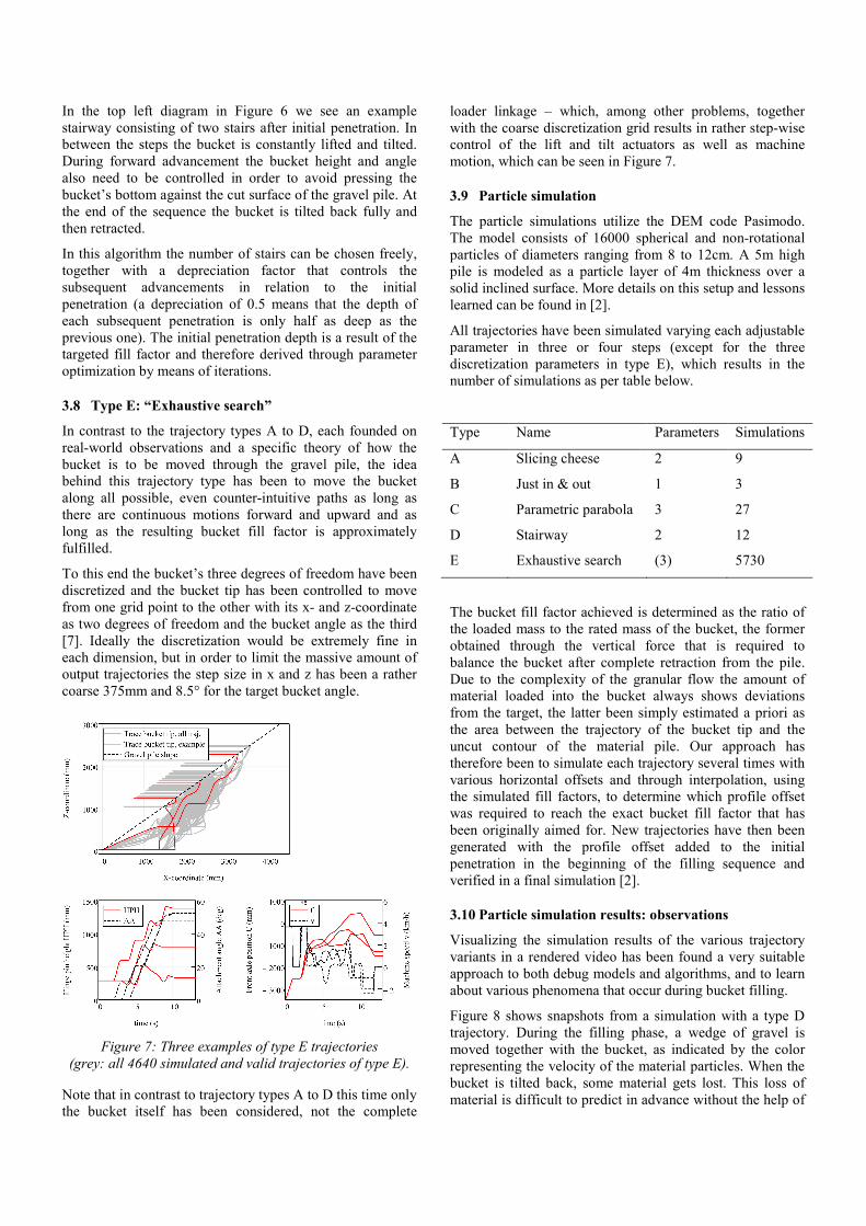
3.8 Type E: “Exhaustive search”

In contrast to the trajectory types A to D, each founded on real-world observations and a specific theory of how the bucket is to be moved through the gravel pile, the idea behind this trajectory type has been to move the bucket along all possible, even counter-intuitive paths as long as there are continuous motions forward and upward and as long as the resulting bucket fill factor is approximately fulfilled.

To this end the bucket’s three degrees of freedom have been discretized and the bucket tip has been controlled to move from one grid point to the other with its x- and z-coordinate as two degrees of freedom and the bucket angle as the third [7]. Ideally the discretization would be extremely fine in each dimension, but in order to limit the massive amount of output trajectories the step size in x and z has been a rather coarse 375mm and 8.5° for the target bucket angle.

Figure 7: Three examples of type E trajectories

(grey: all 4640 simulated and valid trajectories of type E).

Note that in contrast to trajectory types A to D this time only the bucket itself has been considered, not the complete

loader linkage – which, among other problems, together with the coarse discretization grid results in rather step-wise control of the lift and tilt actuators as well as machine motion, which can be seen in Figure 7.

3.9 Particle simulation

The particle simulations utilize the DEM code Pasimodo. The model consists of 16000 spherical and non-rotational particles of diameters ranging from 8 to 12cm. A 5m high pile is modeled as a particle layer of 4m thickness over a solid inclined surface. More details on this setup and lessons learned can be found in [2].

All trajectories have been simulated varying each adjustable parameter in three or four steps (except for the three discretization parameters in type E), which results in the number of simulations as per table below.

Type Name Parameters Simulations

A Slicing cheese 2 9

B Just in & out 1 3

C Parametric parabola 3 27

D Stairway 2 12

E Exhaustive search (3) 5730

The bucket fill factor achieved is determined as the ratio of the loaded mass to the rated mass of the bucket, the former obtained through the vertical force that is required to balance the bucket after complete retraction from the pile. Due to the complexity of the granular flow the amount of material loaded into the bucket always shows deviations from the target, the latter been simply estimated a priori as the area between the trajectory of the bucket tip and the uncut contour of the material pile. Our approach has therefore been to simulate each trajectory several times with various horizontal offsets and through interpolation, using the simulated fill factors, to determine which profile offset was required to reach the exact bucket fill factor that has been originally aimed for. New trajectories have then been generated with the profile offset added to the initial penetration in the beginning of the filling sequence and verified in a final simulation [2].

3.10 Particle simulation results: observations

Visualizing the simulation results of the various trajectory variants in a rendered video has been found a very suitable approach to both debug models and algorithms, and to learn about various phenomena that occur during bucket filling.

Figure 8 shows snapshots from a simulation with a type D trajectory. During the filling phase, a wedge of gravel is moved together with the bucket, as indicated by the color representing the velocity of the material particles. When the bucket is tilted back, some material gets lost. This loss of material is difficult to predict in advance without the help of

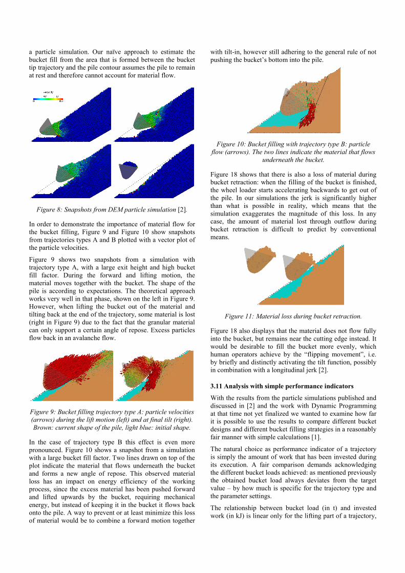
a particle simulation. Our naïve approach to estimate the bucket fill from the area that is formed between the bucket tip trajectory and the pile contour assumes the pile to remain at rest and therefore cannot account for material flow.

Figure 8: Snapshots from DEM particle simulation [2].

In order to demonstrate the importance of material flow for the bucket filling, Figure 9 and Figure 10 show snapshots from trajectories types A and B plotted with a vector plot of the particle velocities.

Figure 9 shows two snapshots from a simulation with trajectory type A, with a large exit height and high bucket fill factor. During the forward and lifting motion, the material moves together with the bucket. The shape of the pile is according to expectations. The theoretical approach works very well in that phase, shown on the left in Figure 9. However, when lifting the bucket out of the material and tilting back at the end of the trajectory, some material is lost (right in Figure 9) due to the fact that the granular material can only support a certain angle of repose. Excess particles flow back in an avalanche flow.

Figure 9: Bucket filling trajectory type A: particle velocities (arrows) during the lift motion (left) and at final tilt (right). Brown: current shape of the pile, light blue: initial shape.

In the case of trajectory type B this effect is even more pronounced. Figure 10 shows a snapshot from a simulation with a large bucket fill factor. Two lines drawn on top of the plot indicate the material that flows underneath the bucket and forms a new angle of repose. This observed material loss has an impact on energy efficiency of the working process, since the excess material has been pushed forward and lifted upwards by the bucket, requiring mechanical energy, but instead of keeping it in the bucket it flows back onto the pile. A way to prevent or at least minimize this loss of material would be to combine a forward motion together

with tilt-in, however still adhering to the general rule of not pushing the bucket’s bottom into the pile.

Figure 10: Bucket filling with trajectory type B: particle flow (arrows). The two lines indicate the material that flows

underneath the bucket.

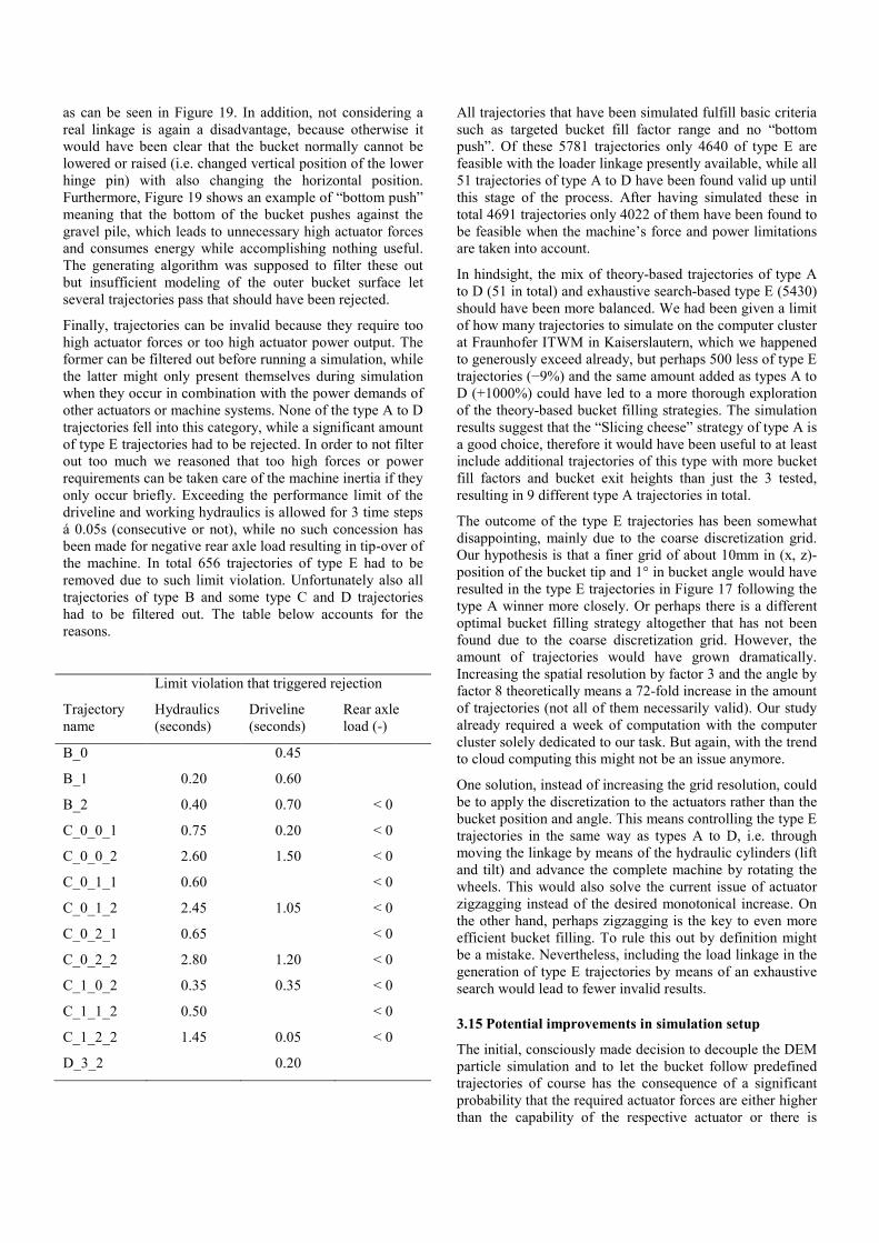
Figure 18 shows that there is also a loss of material during bucket retraction: when the filling of the bucket is finished, the wheel loader starts accelerating backwards to get out of the pile. In our simulations the jerk is significantly higher than what is possible in reality, which means that the simulation exaggerates the magnitude of this loss. In any case, the amount of material lost through outflow during bucket retraction is difficult to predict by conventional means.

Figure 11: Material loss during bucket retraction.

Figure 18 also displays that the material does not flow fully into the bucket, but remains near the cutting edge instead. It would be desirable to fill the bucket more evenly, which human operators achieve by the “flipping movement”, i.e. by briefly and distinctly activating the tilt function, possibly in combination with a longitudinal jerk [2].

3.11 Analysis with simple performance indicators

With the results from the particle simulations published and discussed in [2] and the work with Dynamic Programming at that time not yet finalized we wanted to examine how far it is possible to use the results to compare different bucket designs and different bucket filling strategies in a reasonably fair manner with simple calculations [1].

The natural choice as performance indicator of a trajectory is simply the amount of work that has been invested during its execution. A fair comparison demands acknowledging the different bucket loads achieved: as mentioned previously the obtained bucket load always deviates from the target value – by how much is specific for the trajectory type and the parameter settings.

The relationship between bucket load (in t) and invested work (in kJ) is linear only for the lifting part of a trajectory,

but non-linear for the filling sequence as a whole. This means that while one way to compare trajectories of similar fill factors is to calculate the specific work invested (in kJ/t), a fair comparison between trajectories of significantly different fill factors is more difficult to achieve. It is therefore recommended to plot performance indicators against respective bucket fill factor (i.e. the ratio of achieved bucket load and the bucket rating according to ISO 7546), also when the performance indicator is already normalized to bucket load, such as specific work invested.

We show in [1] that the pure value of the specific work invested in bucket filling is not relevant because it disregards the fact that the achieved result is not only the bucket load itself but also the potential energy achieved by lifting the bucket including its load – which in turn impacts the remainder of the working cycle shown in Figure 1. The height at which the bucket is retracted from the gravel pile thus affects the total energy efficiency of the loading cycle, because it dictates the amount of lifting work still to be performed during driving towards the load receiver, which in turn may affect the driving pattern itself (extension of V to Y). A fair performance indicator must therefore credit the lifting work performed during bucket filling.

One might assume the ratio of the potential energy achieved (affected by bucket load and bucket height) to the work invested can be a suitable performance indicator but we show in [1] that is a poor choice (at least for short loading cycles) because it implies that the sole utility of a bucket filling sequence is a load being lifted. It totally neglects the utility of the bucket actually being filled, which will always require a certain amount of work.

Besides, while the load lifting included in a bucket filling sequence should be credited, it is wrong to assume it to be essential. In a typical short loading cycle there is ample opportunity for lifting to be performed in the phases 2 to 5 (Figure 1) – and in a typical load & carry cycle (not studied here) the lifting is performed right before reaching the load receiver after a transport phase covering a certain distance. To end bucket filling at too great a height in short loading cycles is impractical because the remaining lift work might be so little that even the shortest driving phase to the load receiver will be too long. This might be a waste, also depending on the general question whether it is more efficient to drive and lift concurrently or sequentially (which in turn must be answered for each machine type, i.e. there might be differences for a conventional loader versus the electric series hybrid we have studied). Furthermore, driving and steering a wheel loader with a bucket fully loaded and raised high gives poor machine stability. Most operators therefore raise the bucket to unloading height as late as possible in the cycle, i.e. as close as possible to the load receiver. This also means that loader operators usually don’t leave the pile at too great a bucket height (generally not above the position where the lifting arms are parallel to the ground). The discussed ratio of potential energy achieved and work invested however rewards higher bucket exit heights over lower values for the same bucket load, which shows that it is not a suitable performance indicator [1].

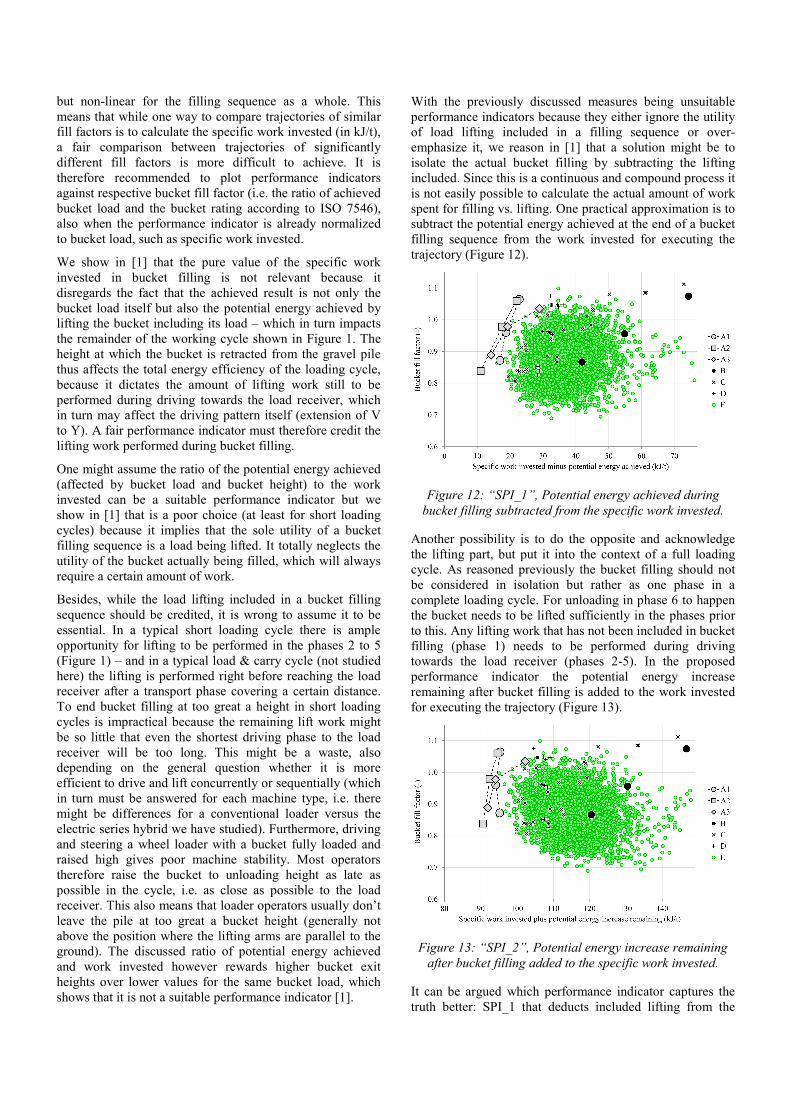
With the previously discussed measures being unsuitable performance indicators because they either ignore the utility of load lifting included in a filling sequence or over-emphasize it, we reason in [1] that a solution might be to isolate the actual bucket filling by subtracting the lifting included. Since this is a continuous and compound process it is not easily possible to calculate the actual amount of work spent for filling vs. lifting. One practical approximation is to subtract the potential energy achieved at the end of a bucket filling sequence from the work invested for executing the trajectory (Figure 12).

Figure 12: “SPI_1”, Potential energy achieved during bucket filling subtracted from the specific work invested.

Another possibility is to do the opposite and acknowledge the lifting part, but put it into the context of a full loading cycle. As reasoned previously the bucket filling should not be considered in isolation but rather as one phase in a complete loading cycle. For unloading in phase 6 to happen the bucket needs to be lifted sufficiently in the phases prior to this. Any lifting work that has not been included in bucket filling (phase 1) needs to be performed during driving towards the load receiver (phases 2-5). In the proposed performance indicator the potential energy increase remaining after bucket filling is added to the work invested for executing the trajectory (Figure 13).

Figure 13: “SPI_2”, Potential energy increase remaining after bucket filling added to the specific work invested.

It can be argued which performance indicator captures the truth better: SPI_1 that deducts included lifting from the

bucket filling sequence by subtracting the amount of potential energy achieved at the end of the trajectory or SPI_2 that acknowledges lifting by adding the increase in potential energy still remaining to be achieved in the subsequent phases of the loading cycle. In both indicators the lifting work invested to achieve an increase in potential energy is assumed without losses, which is a notable simplification.

Also, neither SPI_1 nor SPI_2 as published in [1] include the driveline work, which means that bucket filling sequences resulting in low bucket loads are not suitably punished for poor transport efficiency (basically: the longer the transport section in a working cycle the better it is to fill the bucket as much as possible).

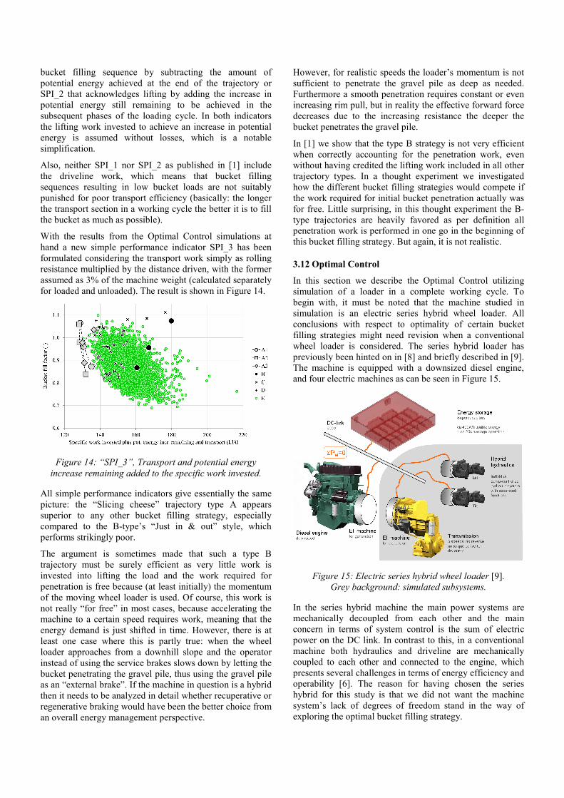
With the results from the Optimal Control simulations at hand a new simple performance indicator SPI_3 has been formulated considering the transport work simply as rolling resistance multiplied by the distance driven, with the former assumed as 3% of the machine weight (calculated separately for loaded and unloaded). The result is shown in Figure 14.

Figure 14: “SPI_3”, Transport and potential energy increase remaining added to the specific work invested.

All simple performance indicators give essentially the same picture: the “Slicing cheese” trajectory type A appears superior to any other bucket filling strategy, especially compared to the B-type’s “Just in & out” style, which performs strikingly poor.

The argument is sometimes made that such a type B trajectory must be surely efficient as very little work is invested into lifting the load and the work required for penetration is free because (at least initially) the momentum of the moving wheel loader is used. Of course, this work is not really “for free” in most cases, because accelerating the machine to a certain speed requires work, meaning that the energy demand is just shifted in time. However, there is at least one case where this is partly true: when the wheel loader approaches from a downhill slope and the operator instead of using the service brakes slows down by letting the bucket penetrating the gravel pile, thus using the gravel pile as an “external brake”. If the machine in question is a hybrid then it needs to be analyzed in detail whether recuperative or regenerative braking would have been the better choice from an overall energy management perspective.

However, for realistic speeds the loader’s momentum is not sufficient to penetrate the gravel pile as deep as needed. Furthermore a smooth penetration requires constant or even increasing rim pull, but in reality the effective forward force decreases due to the increasing resistance the deeper the bucket penetrates the gravel pile.

In [1] we show that the type B strategy is not very efficient when correctly accounting for the penetration work, even without having credited the lifting work included in all other trajectory types. In a thought experiment we investigated how the different bucket filling strategies would compete if the work required for initial bucket penetration actually was for free. Little surprising, in this thought experiment the B-type trajectories are heavily favored as per definition all penetration work is performed in one go in the beginning of this bucket filling strategy. But again, it is not realistic.

3.12 Optimal Control

In this section we describe the Optimal Control utilizing simulation of a loader in a complete working cycle. To begin with, it must be noted that the machine studied in simulation is an electric series hybrid wheel loader. All conclusions with respect to optimality of certain bucket filling strategies might need revision when a conventional wheel loader is considered. The series hybrid loader has previously been hinted on in [8] and briefly described in [9]. The machine is equipped with a downsized diesel engine, and four electric machines as can be seen in Figure 15.

Figure 15: Electric series hybrid wheel loader [9]. Grey background: simulated subsystems.

In the series hybrid machine the main power systems are mechanically decoupled from each other and the main concern in terms of system control is the sum of electric power on the DC link. In contrast to this, in a conventional machine both hydraulics and driveline are mechanically coupled to each other and connected to the engine, which presents several challenges in terms of energy efficiency and operability [6]. The reason for having chosen the series hybrid for this study is that we did not want the machine system’s lack of degrees of freedom stand in the way of exploring the optimal bucket filling strategy.

Dynamic Programming has been used as Optimal Control method. The specific implementation details can be found in [7], but some basic information is necessary to include here: the algorithm developed seeks the global optimum in terms of fuel efficiency, though for practicality converted to electrical actuator energy efficiency – thus excluding the generator set and energy storage, which would be a topic on its own. The simulated subsystems have been marked with a grey background in Figure 15.

For computational efficiency the Optimal Control has been split into four parts:

In part 1 bucket filling, phase 1 in Figure 1, is handled by choosing between the various bucket trajectories. Backward simulation is performed to calculate the energy required for following the trajectories without deviation.

Phases 2 to 5 are covered by the Dynamic Programming algorithm in part 2. Each bucket trajectory from part 1 gives a starting point for part 2, unique in bucket position and load. Optimal Control is performed to find the optimal, i.e. energy-minimizing way to get from the starting point to the point of unloading while maintaining cycle time and thus productivity.

Part 3 covers phase 6, bucket emptying. Ideally this should have been included in part 2 and thus treated individually for each trajectory, because of the different bucket loads. Instead, Optimal Control has been performed one time only to find the minimal energy required to empty a bucket with the load achieved on average with the simulated trajectories. The effect of this is that working cycles with comparatively low bucket load are not suitably punished for the low transport efficiency. However, it is estimated that the impact on the overall conclusions from this study is not severe.

Finally, in part 4 Optimal Control has been performed once for phases 7 to 10, as independent on the chosen bucket filling trajectory from this point on the loader starts always in the same position with the same bucket load (zero) and stops at the same position in front of the gravel pile, ready to start a new working cycle.

The details of the driving cycle in parts 2 and 4, i.e. how long to drive backward/forward, where to reverse, when to steer etc., have not been subject to optimization. Instead, we have used the values from the most energy-efficient operator in the measurements reported in [15] and refer otherwise to previous work [3][4].

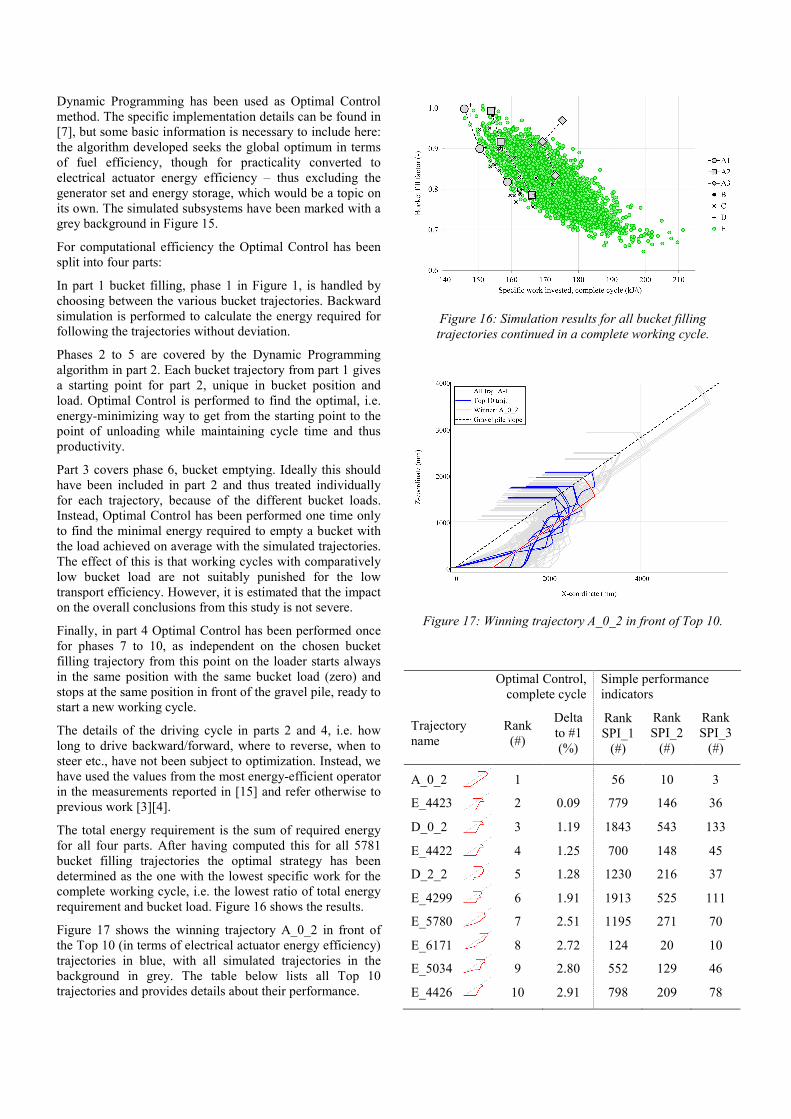
The total energy requirement is the sum of required energy for all four parts. After having computed this for all 5781 bucket filling trajectories the optimal strategy has been determined as the one with the lowest specific work for the complete working cycle, i.e. the lowest ratio of total energy requirement and bucket load. Figure 16 shows the results.

Figure 17 shows the winning trajectory A_0_2 in front of the Top 10 (in terms of electrical actuator energy efficiency) trajectories in blue, with all simulated trajectories in the background in grey. The table below lists all Top 10 trajectories and provides details about their performance.

Figure 16: Simulation results for all bucket filling trajectories continued in a complete working cycle.

Figure 17: Winning trajectory A_0_2 in front of Top 10.

Optimal Control, complete cycle

Simple performance indicators

Trajectory name

Rank (#)

Delta to #1 (%)

Rank SPI_1

(#)

Rank SPI_2

(#)

Rank SPI_3

(#)

A_0_2 1 56 10 3

E_4423 2 0.09 779 146 36

D_0_2 3 1.19 1843 543 133

E_4422 4 1.25 700 148 45

D_2_2 5 1.28 1230 216 37

E_4299 6 1.91 1913 525 111

E_5780 7 2.51 1195 271 70

E_6171 8 2.72 124 20 10

E_5034 9 2.80 552 129 46

E_4426 10 2.91 798 209 78

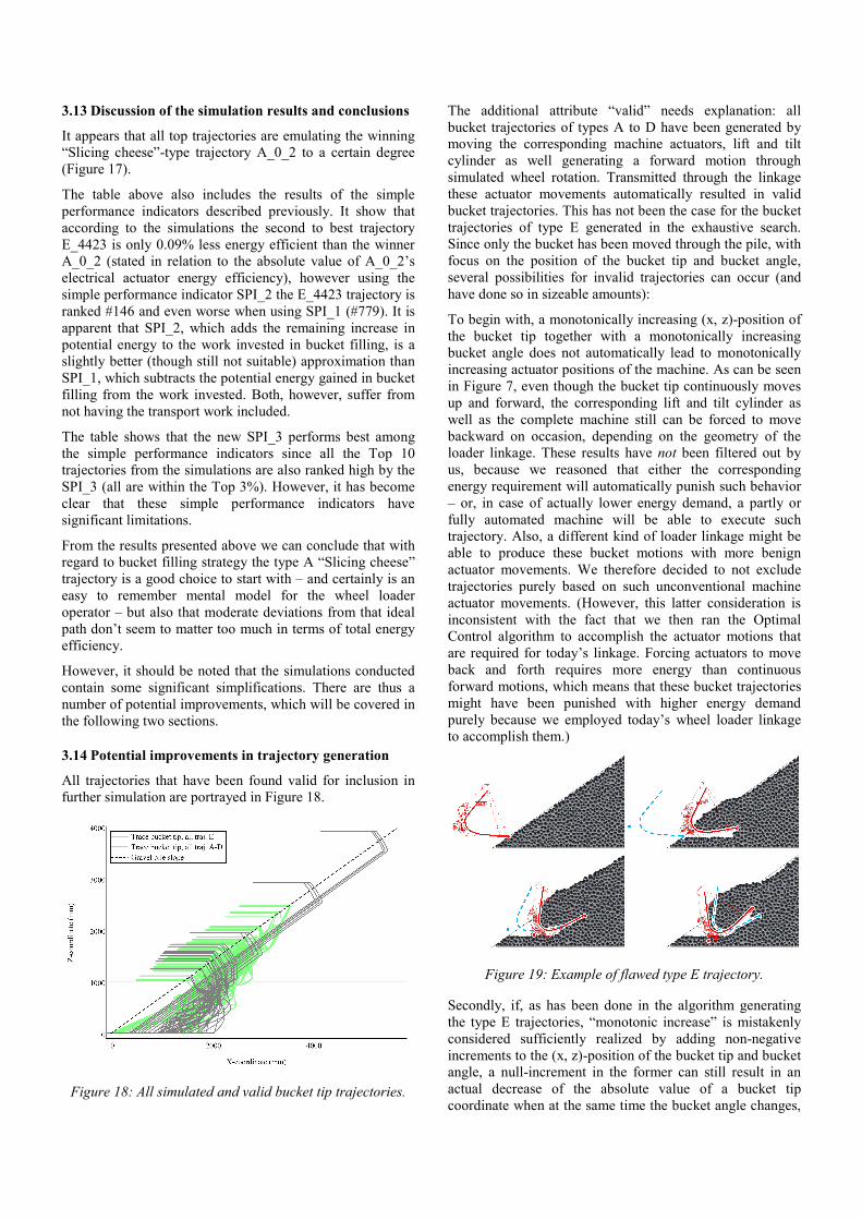
3.13 Discussion of the simulation results and conclusions

It appears that all top trajectories are emulating the winning “Slicing cheese”-type trajectory A_0_2 to a certain degree (Figure 17).

The table above also includes the results of the simple performance indicators described previously. It show that according to the simulations the second to best trajectory E_4423 is only 0.09% less energy efficient than the winner A_0_2 (stated in relation to the absolute value of A_0_2’s electrical actuator energy efficiency), however using the simple performance indicator SPI_2 the E_4423 trajectory is ranked #146 and even worse when using SPI_1 (#779). It is apparent that SPI_2, which adds the remaining increase in potential energy to the work invested in bucket filling, is a slightly better (though still not suitable) approximation than SPI_1, which subtracts the potential energy gained in bucket filling from the work invested. Both, however, suffer from not having the transport work included.

The table shows that the new SPI_3 performs best among the simple performance indicators since all the Top 10 trajectories from the simulations are also ranked high by the SPI_3 (all are within the Top 3%). However, it has become clear that these simple performance indicators have significant limitations.

From the results presented above we can conclude that with regard to bucket filling strategy the type A “Slicing cheese” trajectory is a good choice to start with – and certainly is an easy to remember mental model for the wheel loader operator – but also that moderate deviations from that ideal path don’t seem to matter too much in terms of total energy efficiency.

However, it should be noted that the simulations conducted contain some significant simplifications. There are thus a number of potential improvements, which will be covered in the following two sections.

3.14 Potential improvements in trajectory generation

All trajectories that have been found valid for inclusion in further simulation are portrayed in Figure 18.

Figure 18: All simulated and valid bucket tip trajectories.

The additional attribute “valid” needs explanation: all bucket trajectories of types A to D have been generated by moving the corresponding machine actuators, lift and tilt cylinder as well generating a forward motion through simulated wheel rotation. Transmitted through the linkage these actuator movements automatically resulted in valid bucket trajectories. This has not been the case for the bucket trajectories of type E generated in the exhaustive search. Since only the bucket has been moved through the pile, with focus on the position of the bucket tip and bucket angle, several possibilities for invalid trajectories can occur (and have done so in sizeable amounts):

To begin with, a monotonically increasing (x, z)-position of the bucket tip together with a monotonically increasing bucket angle does not automatically lead to monotonically increasing actuator positions of the machine. As can be seen in Figure 7, even though the bucket tip continuously moves up and forward, the corresponding lift and tilt cylinder as well as the complete machine still can be forced to move backward on occasion, depending on the geometry of the loader linkage. These results have not been filtered out by us, because we reasoned that either the corresponding energy requirement will automatically punish such behavior – or, in case of actually lower energy demand, a partly or fully automated machine will be able to execute such trajectory. Also, a different kind of loader linkage might be able to produce these bucket motions with more benign actuator movements. We therefore decided to not exclude trajectories purely based on such unconventional machine actuator movements. (However, this latter consideration is inconsistent with the fact that we then ran the Optimal Control algorithm to accomplish the actuator motions that are required for today’s linkage. Forcing actuators to move back and forth requires more energy than continuous forward motions, which means that these bucket trajectories might have been punished with higher energy demand purely because we employed today’s wheel loader linkage to accomplish them.)

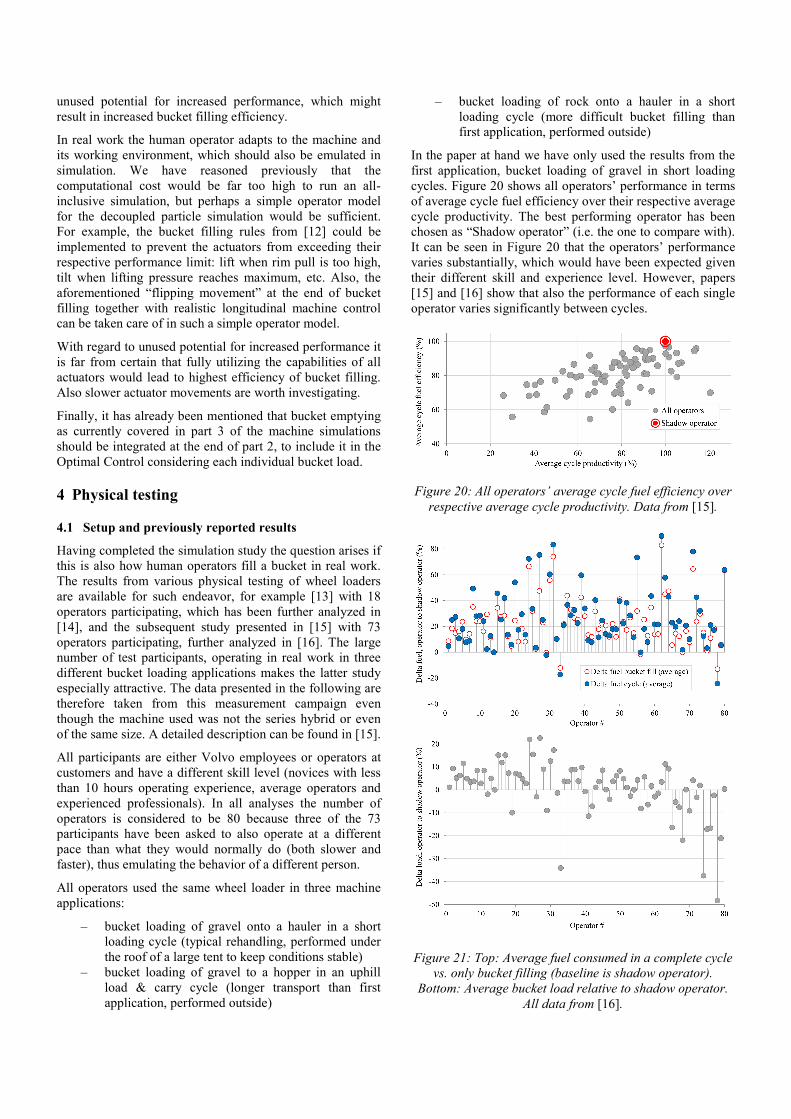
Figure 19: Example of flawed type E trajectory.

Secondly, if, as has been done in the algorithm generating the type E trajectories, “monotonic increase” is mistakenly considered sufficiently realized by adding non-negative increments to the (x, z)-position of the bucket tip and bucket angle, a null-increment in the former can still result in an actual decrease of the absolute value of a bucket tip coordinate when at the same time the bucket angle changes,

as can be seen in Figure 19. In addition, not considering a real linkage is again a disadvantage, because otherwise it would have been clear that the bucket normally cannot be lowered or raised (i.e. changed vertical position of the lower hinge pin) with also changing the horizontal position. Furthermore, Figure 19 shows an example of “bottom push” meaning that the bottom of the bucket pushes against the gravel pile, which leads to unnecessary high actuator forces and consumes energy while accomplishing nothing useful. The generating algorithm was supposed to filter these out but insufficient modeling of the outer bucket surface let several trajectories pass that should have been rejected.

Finally, trajectories can be invalid because they require too high actuator forces or too high actuator power output. The former can be filtered out before running a simulation, while the latter might only present themselves during simulation when they occur in combination with the power demands of other actuators or machine systems. None of the type A to D trajectories fell into this category, while a significant amount of type E trajectories had to be rejected. In order to not filter out too much we reasoned that too high forces or power requirements can be taken care of the machine inertia if they only occur briefly. Exceeding the performance limit of the driveline and working hydraulics is allowed for 3 time steps á 0.05s (consecutive or not), while no such concession has been made for negative rear axle load resulting in tip-over of the machine. In total 656 trajectories of type E had to be removed due to such limit violation. Unfortunately also all trajectories of type B and some type C and D trajectories had to be filtered out. The table below accounts for the reasons.

Limit violation that triggered rejection

Trajectory name

Hydraulics (seconds)

Driveline (seconds)

Rear axle load (-)

B_0 0.45

B_1 0.20 0.60

B_2 0.40 0.70 < 0

C_0_0_1 0.75 0.20 < 0

C_0_0_2 2.60 1.50 < 0

C_0_1_1 0.60 < 0

C_0_1_2 2.45 1.05 < 0

C_0_2_1 0.65 < 0

C_0_2_2 2.80 1.20 < 0

C_1_0_2 0.35 0.35 < 0

C_1_1_2 0.50 < 0

C_1_2_2 1.45 0.05 < 0

D_3_2 0.20

All trajectories that have been simulated fulfill basic criteria such as targeted bucket fill factor range and no “bottom push”. Of these 5781 trajectories only 4640 of type E are feasible with the loader linkage presently available, while all 51 trajectories of type A to D have been found valid up until this stage of the process. After having simulated these in total 4691 trajectories only 4022 of them have been found to be feasible when the machine’s force and power limitations are taken into account.

In hindsight, the mix of theory-based trajectories of type A to D (51 in total) and exhaustive search-based type E (5430) should have been more balanced. We had been given a limit of how many trajectories to simulate on the computer cluster at Fraunhofer ITWM in Kaiserslautern, which we happened to generously exceed already, but perhaps 500 less of type E trajectories (−9%) and the same amount added as types A to D (+1000%) could have led to a more thorough exploration of the theory-based bucket filling strategies. The simulation results suggest that the “Slicing cheese” strategy of type A is a good choice, therefore it would have been useful to at least include additional trajectories of this type with more bucket fill factors and bucket exit heights than just the 3 tested, resulting in 9 different type A trajectories in total.

The outcome of the type E trajectories has been somewhat disappointing, mainly due to the coarse discretization grid. Our hypothesis is that a finer grid of about 10mm in (x, z)-position of the bucket tip and 1° in bucket angle would have resulted in the type E trajectories in Figure 17 following the type A winner more closely. Or perhaps there is a different optimal bucket filling strategy altogether that has not been found due to the coarse discretization grid. However, the amount of trajectories would have grown dramatically. Increasing the spatial resolution by factor 3 and the angle by factor 8 theoretically means a 72-fold increase in the amount of trajectories (not all of them necessarily valid). Our study already required a week of computation with the computer cluster solely dedicated to our task. But again, with the trend to cloud computing this might not be an issue anymore.

One solution, instead of increasing the grid resolution, could be to apply the discretization to the actuators rather than the bucket position and angle. This means controlling the type E trajectories in the same way as types A to D, i.e. through moving the linkage by means of the hydraulic cylinders (lift and tilt) and advance the complete machine by rotating the wheels. This would also solve the current issue of actuator zigzagging instead of the desired monotonical increase. On the other hand, perhaps zigzagging is the key to even more efficient bucket filling. To rule this out by definition might be a mistake. Nevertheless, including the load linkage in the generation of type E trajectories by means of an exhaustive search would lead to fewer invalid results.

3.15 Potential improvements in simulation setup

The initial, consciously made decision to decouple the DEM particle simulation and to let the bucket follow predefined trajectories of course has the consequence of a significant probability that the required actuator forces are either higher than the capability of the respective actuator or there is

unused potential for increased performance, which might result in increased bucket filling efficiency.

In real work the human operator adapts to the machine and its working environment, which should also be emulated in simulation. We have reasoned previously that the computational cost would be far too high to run an all-inclusive simulation, but perhaps a simple operator model for the decoupled particle simulation would be sufficient. For example, the bucket filling rules from [12] could be implemented to prevent the actuators from exceeding their respective performance limit: lift when rim pull is too high, tilt when lifting pressure reaches maximum, etc. Also, the aforementioned “flipping movement” at the end of bucket filling together with realistic longitudinal machine control can be taken care of in such a simple operator model.

With regard to unused potential for increased performance it is far from certain that fully utilizing the capabilities of all actuators would lead to highest efficiency of bucket filling. Also slower actuator movements are worth investigating.

Finally, it has already been mentioned that bucket emptying as currently covered in part 3 of the machine simulations should be integrated at the end of part 2, to include it in the Optimal Control considering each individual bucket load.

4 Physical testing

4.1 Setup and previously reported results

Having completed the simulation study the question arises if this is also how human operators fill a bucket in real work. The results from various physical testing of wheel loaders are available for such endeavor, for example [13] with 18 operators participating, which has been further analyzed in [14], and the subsequent study presented in [15] with 73 operators participating, further analyzed in [16]. The large number of test participants, operating in real work in three different bucket loading applications makes the latter study especially attractive. The data presented in the following are therefore taken from this measurement campaign even though the machine used was not the series hybrid or even of the same size. A detailed description can be found in [15].

All participants are either Volvo employees or operators at customers and have a different skill level (novices with less than 10 hours operating experience, average operators and experienced professionals). In all analyses the number of operators is considered to be 80 because three of the 73 participants have been asked to also operate at a different pace than what they would normally do (both slower and faster), thus emulating the behavior of a different person.

All operators used the same wheel loader in three machine applications:

‒ bucket loading of gravel onto a hauler in a short loading cycle (typical rehandling, performed under the roof of a large tent to keep conditions stable)

‒ bucket loading of gravel to a hopper in an uphill load & carry cycle (longer transport than first application, performed outside)

‒ bucket loading of rock onto a hauler in a short loading cycle (more difficult bucket filling than first application, performed outside)

In the paper at hand we have only used the results from the first application, bucket loading of gravel in short loading cycles. Figure 20 shows all operators’ performance in terms of average cycle fuel efficiency over their respective average cycle productivity. The best performing operator has been chosen as “Shadow operator” (i.e. the one to compare with). It can be seen in Figure 20 that the operators’ performance varies substantially, which would have been expected given their different skill and experience level. However, papers [15] and [16] show that also the performance of each single operator varies significantly between cycles.

Figure 20: All operators’ average cycle fuel efficiency over respective average cycle productivity. Data from [15].

Figure 21: Top: Average fuel consumed in a complete cycle vs. only bucket filling (baseline is shadow operator).

Bottom: Average bucket load relative to shadow operator. All data from [16].

The diagram in the top of Figure 21 shows with blue dots how much more fuel each operator consumes on average per cycle in comparison to the Shadow operator (normalized to 100%. The red rings in the plot show how much the bucket filling phase contributes to that additional fuel consumption per cycle. Some operators manage to consume less fuel than the most efficient Shadow operator, but the bottom diagram reveals that this is due to an even lesser bucket load (i.e. in terms of fuel efficiency they are still worse than the Shadow operator as their decrease in fuel consumption is less than their decrease in bucket load). Figure 21 confirms previous reporting [6] that bucket filling is the predominant phase in a short loading cycle when it comes to fuel efficiency.

In the context of the paper at hand it is of interest to examine whether the data from [15] can support the conclusion that following the “Slicing cheese” strategy for filling the bucket leads to an efficient (if not the most efficient) short loading cycle for a wheel loader working in gravel.

4.2 Analysis of bucket filling trajectories

The large number of data acquired in this measurement campaign necessitates an automatic analysis, one important aspect of this being the ability to automatically extract the bucket filling phase from a continuous series of time data. Ideally the location of the machine in relation to the gravel pile would be among the signals recorded (and in high resolution). However, this has not been the case. In any case the location of the gravel pile is ever changing since material is constantly removed by the wheel loader, yet more material might fall down from the pile’s top like a landslide.

A solution might be to record the loading cycle on video and let automatic motion capture take care of locating both bucket and pile. In the simplest version this would be done from the side of the pile, but the constantly changing shape of the gravel pile’s front might be a problem (and a loading pocket with transparent side walls seems far-fetched). Filming from a different angle with stereo cameras or time-of-flight cameras might solve this problem, but requires sophisticated image analysis. The measurement setup we used did include a forward-facing camera in the wheel loader cab, but the frame rate of 1fps and the fish-eye lens employed make the recorded video feed unsuitable for precise automatic determination of when and where bucket filling started. Also, the camera is moving with the machine and the image is therefore somewhat shaky.

Solutions for automatic detection of loading cycle phases such as bucket filling have been published [13][17][18], though it turned out that each of the underlying assumptions have been violated in our case. For example, it is not possible to let the gear shift F2→F1 (forward 2 down to 1) mark the beginning of the bucket filling or even use it to search back in time to find the beginning, because some operators such as the Shadow operator “EP15” prefer to manually activate the kick-down function. Also, each operator is unique in how deep the gravel pile is initially penetrated and how fast – both factors affect the resistance and thus the required traction force, which in turn affects

when the automatic kick-down function triggers the gear shift. Basing the beginning of the bucket filling phase on this gear shift is therefore not reliable.

Another possibility seems to be to set the gear shift F1→R2 (forward 1 to reverse 2) as the end of bucket filling and normalize all filling sequences to this point in time and space. However, all operators penetrate the pile differently and to unique depths, which makes it impossible to use this to find when the bucket filling actually started.

In [13] the beginning of bucket filling is defined by the operator laying the bucket flat on the ground and not touching the hydraulic levers again until after the initial penetration of the gravel pile. In the measurements used here some operators lay the bucket down very early, farther away from the gravel pile than others – thus invalidating this possibility, too. In addition, we discovered that due to the specific setup for data acquisition the recorded signals for lift and tilt position have a varying and overall rather poor sampling rate, mostly 10Hz but sometimes as low as 1Hz.

Finally, a significantly increased torque output of the engine might indicate the beginning of bucket filling – yet again, all operators act differently and while some almost operate in a stop-motion fashion others keep all actuators moving all the time. The torque output of the engine is determined by the requirements of hydraulics and driveline, which in turn both are largely affected by the operator’s use of the machine.

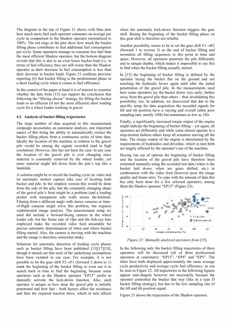
Having run out of options the beginning of bucket filling and the location of the gravel pile have therefore been estimated manually using the recorded test data (when is the bucket laid down, when are gears shifted, etc.) in combination with the video feed (however poor the image quality and frame rate). To cope with the amount of data this has only been done for a few selected operators, among them the Shadow operator “EP15” (Figure 22).

Figure 22: Manually analyzed operators from [15].

In the following only the bucket filling trajectories of three operators will be discussed (all of them professional operators at customers): “EP15”, “EP4” and “EP5”. The latter have both displayed approximately the same average cycle productivity and average cycle fuel efficiency, as can be seen in Figure 22. All trajectories in the following figures appear stair-shaped, however not necessarily because the operator controlled the bucket that way (like in a type D bucket filling strategy), but due to the low sampling rate of the lift and tilt position signal.

Figure 23 shows the trajectories of the Shadow operator.

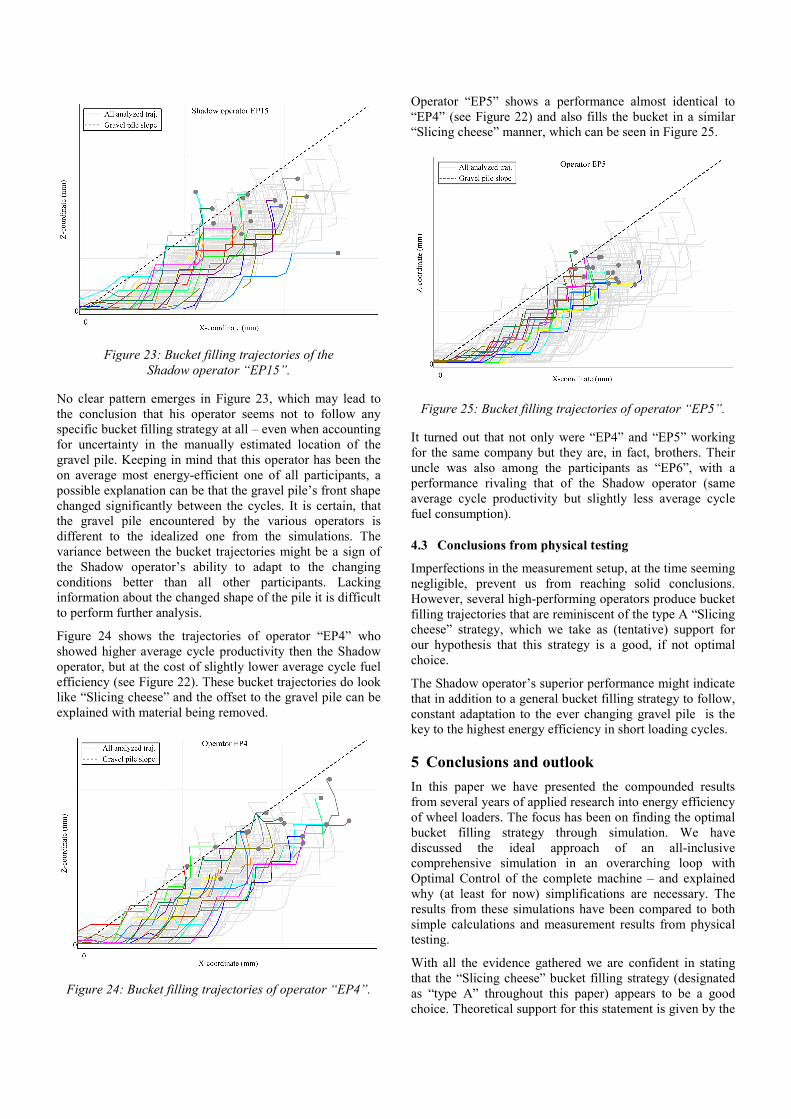
Figure 23: Bucket filling trajectories of the Shadow operator “EP15”.

No clear pattern emerges in Figure 23, which may lead to the conclusion that his operator seems not to follow any specific bucket filling strategy at all – even when accounting for uncertainty in the manually estimated location of the gravel pile. Keeping in mind that this operator has been the on average most energy-efficient one of all participants, a possible explanation can be that the gravel pile’s front shape changed significantly between the cycles. It is certain, that the gravel pile encountered by the various operators is different to the idealized one from the simulations. The variance between the bucket trajectories might be a sign of the Shadow operator’s ability to adapt to the changing conditions better than all other participants. Lacking information about the changed shape of the pile it is difficult to perform further analysis.

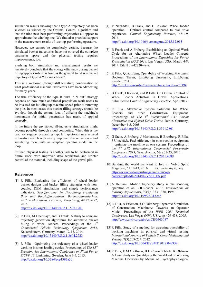
Figure 24 shows the trajectories of operator “EP4” who showed higher average cycle productivity then the Shadow operator, but at the cost of slightly lower average cycle fuel efficiency (see Figure 22). These bucket trajectories do look like “Slicing cheese” and the offset to the gravel pile can be explained with material being removed.

Figure 24: Bucket filling trajectories of operator “EP4”.

Operator “EP5” shows a performance almost identical to “EP4” (see Figure 22) and also fills the bucket in a similar “Slicing cheese” manner, which can be seen in Figure 25.

Figure 25: Bucket filling trajectories of operator “EP5”.

It turned out that not only were “EP4” and “EP5” working for the same company but they are, in fact, brothers. Their uncle was also among the participants as “EP6”, with a performance rivaling that of the Shadow operator (same average cycle productivity but slightly less average cycle fuel consumption).

4.3 Conclusions from physical testing

Imperfections in the measurement setup, at the time seeming negligible, prevent us from reaching solid conclusions. However, several high-performing operators produce bucket filling trajectories that are reminiscent of the type A “Slicing cheese” strategy, which we take as (tentative) support for our hypothesis that this strategy is a good, if not optimal choice.

The Shadow operator’s superior performance might indicate that in addition to a general bucket filling strategy to follow, constant adaptation to the ever changing gravel pile is the key to the highest energy efficiency in short loading cycles.

5 Conclusions and outlook In this paper we have presented the compounded results from several years of applied research into energy efficiency of wheel loaders. The focus has been on finding the optimal bucket filling strategy through simulation. We have discussed the ideal approach of an all-inclusive comprehensive simulation in an overarching loop with Optimal Control of the complete machine – and explained why (at least for now) simplifications are necessary. The results from these simulations have been compared to both simple calculations and measurement results from physical testing.

With all the evidence gathered we are confident in stating that the “Slicing cheese” bucket filling strategy (designated as “type A” throughout this paper) appears to be a good choice. Theoretical support for this statement is given by the

simulation results showing that a type A trajectory has been selected as winner by the Optimal Control algorithm and that the nine next best performing trajectories all appear to approximate the winning one. We find also practical support in the measurement results of two top-performing operators.

However, we cannot be completely certain, because the simulated bucket trajectories have not covered the complete parameter space and the physical testing requires improvements, too.

Studying both simulation and measurement results we tentatively conclude that the energy efficiency during bucket filling appears robust as long as the general trend is a bucket trajectory of type A “Slicing cheese”.

This is a welcome (though still tentative) confirmation of what professional machine instructors have been advocating for many years.

The true efficiency of the type B “Just in & out” strategy depends on how much additional propulsion work needs to be invested for building up machine speed prior to ramming the pile. In most cases this bucket filling strategy should be avoided, though the general idea of utilizing the machine’s momentum for initial penetration has merit, if applied correctly.

In the future the envisioned all-inclusive simulations might become possible through cloud computing. When this is the case we suggest generating type E trajectories in a revised exhaustive search with vastly improved discretization – and simulating these with an adaptive operator model in the loop.

Refined physical testing is another task to be performed in future work, with improved data acquisition and stricter control of the material, including shape of the gravel pile.

References [1] R Filla. Evaluating the efficiency of wheel loader

bucket designs and bucket filling strategies with non-coupled DEM simulations and simple performance indicators. Schriftenreihe der Forschungsvereinigung Bau- und Baustoffmaschinen: Baumaschinentechnik 2015 – Maschinen, Prozesse, Vernetzung, 49:273-292, 2015. http://dx.doi.org/10.13140/RG.2.1.1507.1201

[2] R Filla, M Obermayr, and B Frank. A study to compare trajectory generation algorithms for automatic bucket filling in wheel loaders. Proceedings of the 3rd Commercial Vehicle Technology Symposium 2014, Kaiserslautern, Germany, March 12-13, 2014. http://dx.doi.org/10.13140/RG.2.1.3604.2723

[3] R Filla. Optimizing the trajectory of a wheel loader working in short loading cycles. Proceedings of The 13th Scandinavian International Conference on Fluid Power SICFP’13, Linköping, Sweden, June 3-5, 2013. http://dx.doi.org/10.3384/ecp1392a30

[4] V Nezhadali, B Frank, and L Eriksson. Wheel loader operation – Optimal control compared to real drive experience. Control Engineering Practice, 48:1-9, 2016. http://dx.doi.org/10.1016/j.conengprac.2015.12.015

[5] B Frank and A Fröberg. Establishing an Optimal Work Cycle for an Alternative Wheel Loader Concept. Proceedings of the International Exposition for Power Transmission IFPE 2014, Las Vegas, USA, March 4-8, 2014. ISBN 0-942220-49-8.

[6] R Filla. Quantifying Operability of Working Machines. Doctoral Thesis, Linköping University, Linköping, Sweden, 2011. http://urn.kb.se/resolve?urn=urn:nbn:se:liu:diva-70394

[7] B Frank, J Kleinert, and R Filla. On Optimal Control of Wheel Loader Actuators in Gravel Applications. Submitted to Control Engineering Practice, April 2017.

[8] R Filla. Alternative System Solutions for Wheel Loaders and other Construction Equipment. Proceedings of The 1st International CTI Forum Alternative and Hybrid Drive Trains, Berlin, Germany, December 4-5, 2008. http://dx.doi.org/10.13140/RG.2.1.3391.2801

[9] G Stein, A Fröberg, J Martinsson, B Brattberg, R Filla, J Unnebäck. Fuel efficiency in construction equipment – optimize the machine as one system. Proceedings of the 7th AVL International Commercial Powertrain Conference 2013, Graz, Austria, May 22-23, 2013. http://dx.doi.org/10.13140/RG.2.1.2031.4089

[10] Building the world we want to live in. Volvo Spirit Magazine, 61:10-13, 2016. (URL verified May 17, 2017) https://www.volvospiritmagazine.com/wp-content/uploads/2014/02/VS61_EN.pdf

[11] A Hemami. Motion trajectory study in the scooping operation of an LHD-loader. IEEE Transactions on Industry Applications, 30(5):1333-1338, 1994. http://dx.doi.org/10.1109/28.315248

[12] R Filla, A Ericsson, J-O Palmberg. Dynamic Simulation of Construction Machinery: Towards an Operator Model. Proceedings of the IFPE 2005 Technical Conference, Las Vegas (NV), USA, pp 429-438, 2005. http://www.arxiv.org/abs/cs.CE/0503087

[13] R Filla. Study of a method for assessing operability of working machines in physical and virtual testing. International Journal of Vehicle Systems Modelling and Testing, 7(3):209-234, 2012. http://dx.doi.org/10.1504/IJVSMT.2012.048939

[14] R Filla, E M G Olsson, B H C von Schéele, K Ohlsson. A Case Study on Quantifying the Workload of Working Machine Operators by Means of Psychophysiological

Measurements. The 13th Scandinavian International Conference on Fluid Power SICFP’13, Linköping, Sweden, June 3-5, 2013. http://dx.doi.org/10.3384/ecp1392a29

[15] B Frank, L Skogh, M Alaküla. On wheel loader fuel efficiency difference due to operator behaviour distribution. Proceedings of the 2nd Commercial Vehicle Technology Symposium 2012, Kaiserslautern, Germany, March 13-15, 2012. (URL verified May 17, 2017) http://www.iea.lth.se/publications/Papers/Frank_2012.pdf

[16] B Frank, L Skogh, R Filla, M Alaküla. On increasing fuel efficiency by operator assistant systems in a wheel loader. Proceedings of the 2012 International Conference on Advanced Vehicle Technologies and Integration, Changchun, China, July 16-19, 2012, pp. 155-161. ISBN 978-7-111-39909-4. http://dx.doi.org/10.13140/RG.2.1.3129.1362

[17] K Ohlsson-Öhman. Identifying operator usage of wheel loaders utilizing pattern recognition techniques. Master thesis, Division of Automatic Control, Department of Electrical Engineering, Linköping University, Linköping, Sweden, 2012. http://urn.kb.se/resolve?urn=urn:nbn:se:liu:diva-78937

[18] T Nilsson, P Nyberg, C Sundström, E Frisk and M Krysander. Robust Driving Pattern Detection and Identification with a Wheel Loader Application. International journal of vehicle systems modelling and testing, 1(9):56-76, 2014. http://dx.doi.org/10.1504/IJVSMT.2014.059156