DeconstructingSfM-Net architectureand beyond

Deep Learning for Structure-from-Motion (SfM)

Purpose of this presentation

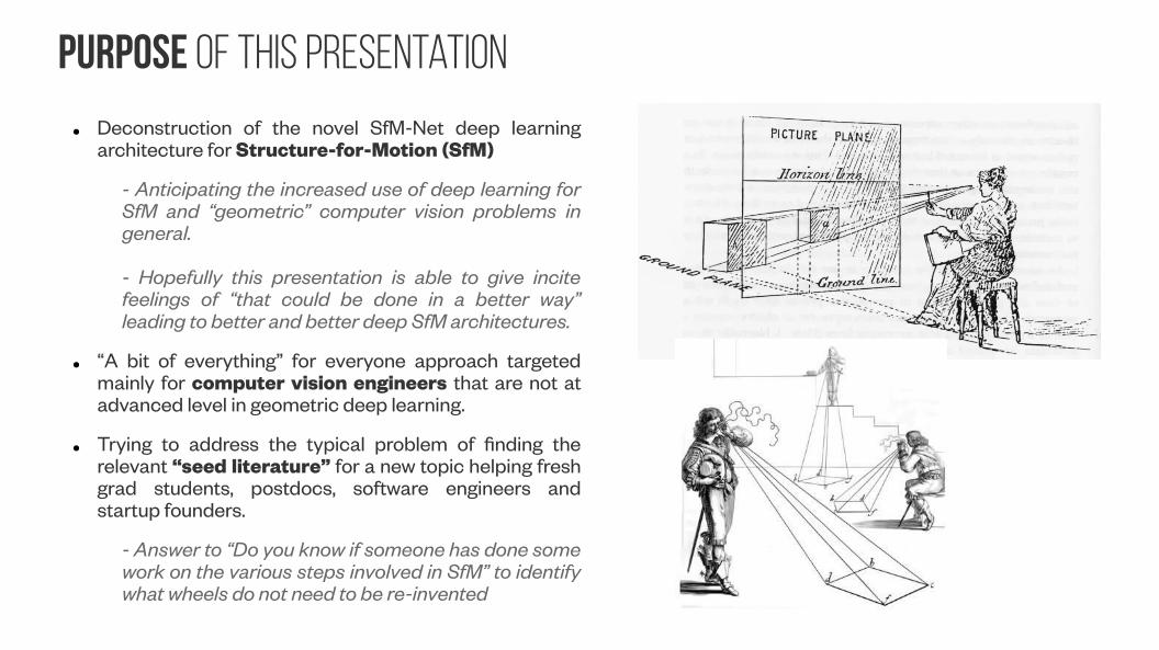
● Deconstruction of the novel SfM-Net deep learning architecture for Structure-for-Motion (SfM)

- Anticipating the increased use of deep learning for SfM and “geometric” computer vision problems in general.

- Hopefully this presentation is able to give incite feelings of “that could be done in a better way” leading to better and better deep SfM architectures.

● “A bit of everything” for everyone approach targeted mainly for computer vision engineers that are not at advanced level in geometric deep learning.

● Trying to address the typical problem of finding the relevant “seed literature” for a new topic helping fresh grad students, postdocs, software engineers and startup founders.

- Answer to “Do you know if someone has done some work on the various steps involved in SfM” to identify what wheels do not need to be re-invented

Background

SfM • Structure from Motion Basics recap • Camera Projections

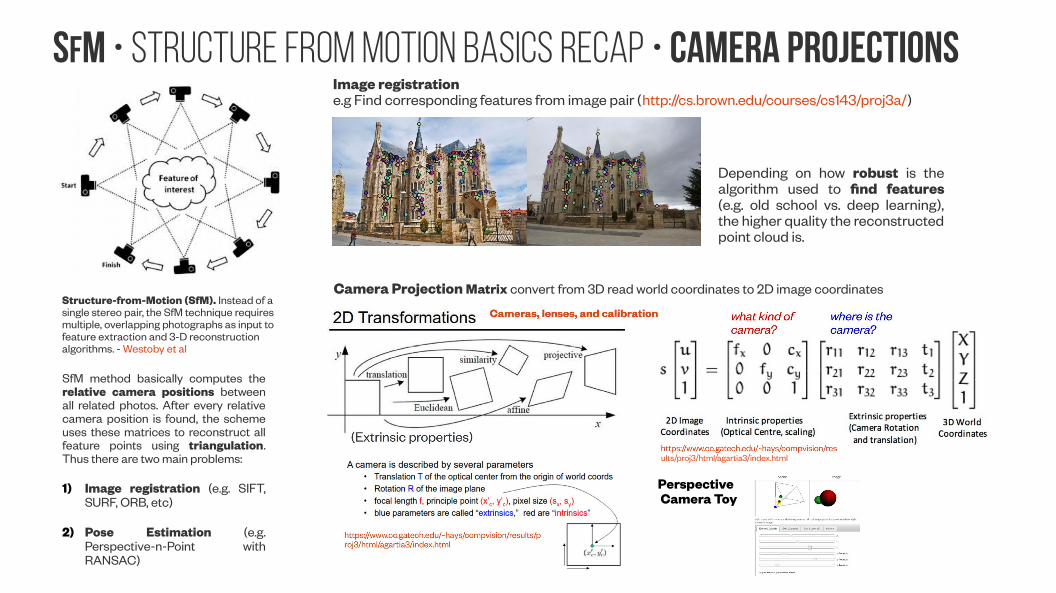
Structure-from-Motion (SfM). Instead of a single stereo pair, the SfM technique requires multiple, overlapping photographs as input to feature extraction and 3-D reconstruction algorithms. - Westoby et al

SfM method basically computes the relative camera positions between all related photos. After every relative camera position is found, the scheme uses these matrices to reconstruct all feature points using triangulation. Thus there are two main problems:

1) Image registration (e.g. SIFT, SURF, ORB, etc)

2) Pose Estimation (e.g. Perspective-n-Point with RANSAC)

Image registratione.g Find corresponding features from image pair (http://cs.brown.edu/courses/cs143/proj3a/)

Depending on how robust is the algorithm used to find features (e.g. old school vs. deep learning), the higher quality the reconstructed point cloud is.

Camera Projection Matrix convert from 3D read world coordinates to 2D image coordinates

ults/proj3/html/agartia3/index.html

Perspective Camera Toy

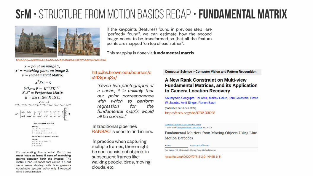
SfM • Structure from Motion Basics recap • Fundamental Matrix

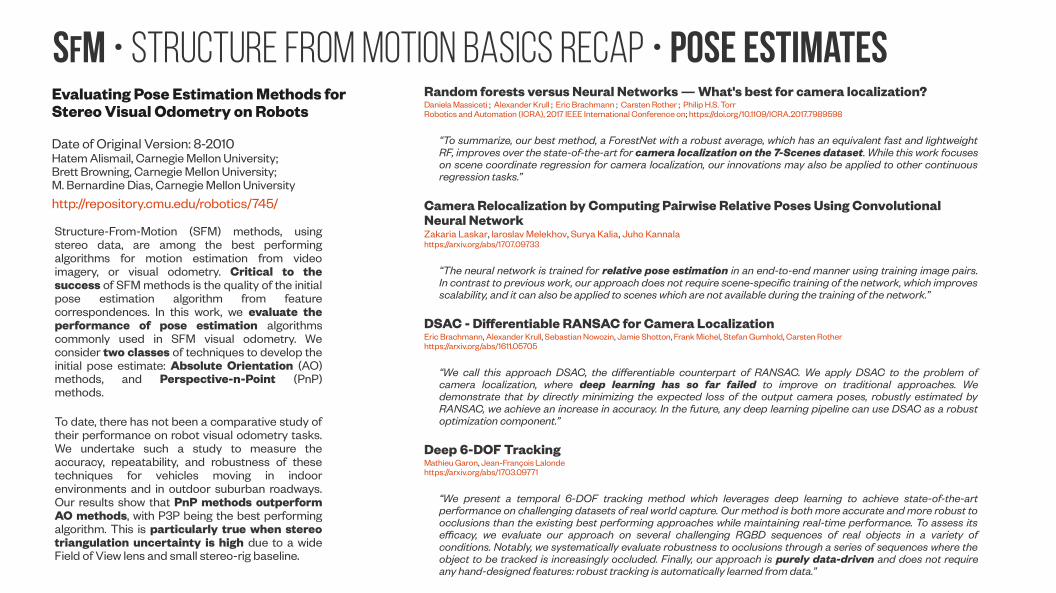
SfM • Structure from Motion Basics recap • pose estimatesEvaluating Pose Estimation Methods forStereo Visual Odometry on Robots

Date of Original Version: 8-2010Hatem Alismail, Carnegie Mellon University; Brett Browning, Carnegie Mellon University;M. Bernardine Dias, Carnegie Mellon University

http://repository.cmu.edu/robotics/745/

Structure-From-Motion (SFM) methods, using stereo data, are among the best performing algorithms for motion estimation from video imagery, or visual odometry. Critical to the success of SFM methods is the quality of the initial pose estimation algorithm from feature correspondences. In this work, we evaluate the performance of pose estimation algorithms commonly used in SFM visual odometry. We consider two classes of techniques to develop the initial pose estimate: Absolute Orientation (AO) methods, and Perspective-n-Point (PnP) methods.

To date, there has not been a comparative study of their performance on robot visual odometry tasks. We undertake such a study to measure the accuracy, repeatability, and robustness of these techniques for vehicles moving in indoor environments and in outdoor suburban roadways. Our results show that PnP methods outperform AO methods, with P3P being the best performing algorithm. This is particularly true when stereo triangulation uncertainty is high due to a wide Field of View lens and small stereo-rig baseline.

Random forests versus Neural Networks — What's best for camera localization?Daniela Massiceti ; Alexander Krull ; Eric Brachmann ; Carsten Rother ; Philip H.S. TorrRobotics and Automation (ICRA), 2017 IEEE International Conference on; https://doi.org/10.1109/ICRA.2017.7989598

“To summarize, our best method, a ForestNet with a robust average, which has an equivalent fast and lightweight RF, improves over the state-of-the-art for camera localization on the 7-Scenes dataset. While this work focuses on scene coordinate regression for camera localization, our innovations may also be applied to other continuous regression tasks.”

Camera Relocalization by Computing Pairwise Relative Poses Using Convolutional Neural NetworkZakaria Laskar, Iaroslav Melekhov, Surya Kalia, Juho Kannalahttps://arxiv.org/abs/1707.09733

“The neural network is trained for relative pose estimation in an end-to-end manner using training image pairs. In contrast to previous work, our approach does not require scene-specific training of the network, which improves scalability, and it can also be applied to scenes which are not available during the training of the network.”

DSAC - Differentiable RANSAC for Camera LocalizationEric Brachmann, Alexander Krull, Sebastian Nowozin, Jamie Shotton, Frank Michel, Stefan Gumhold, Carsten Rotherhttps://arxiv.org/abs/1611.05705

“We call this approach DSAC, the differentiable counterpart of RANSAC. We apply DSAC to the problem of camera localization, where deep learning has so far failed to improve on traditional approaches. We demonstrate that by directly minimizing the expected loss of the output camera poses, robustly estimated by RANSAC, we achieve an increase in accuracy. In the future, any deep learning pipeline can use DSAC as a robust optimization component.”

Deep 6-DOF TrackingMathieu Garon, Jean-François Lalondehttps://arxiv.org/abs/1703.09771

“We present a temporal 6-DOF tracking method which leverages deep learning to achieve state-of-the-art performance on challenging datasets of real world capture. Our method is both more accurate and more robust to occlusions than the existing best performing approaches while maintaining real-time performance. To assess its efficacy, we evaluate our approach on several challenging RGBD sequences of real objects in a variety of conditions. Notably, we systematically evaluate robustness to occlusions through a series of sequences where the object to be tracked is increasingly occluded. Finally, our approach is purely data-driven and does not require any hand-designed features: robust tracking is automatically learned from data.”

SfM-Net • Intro

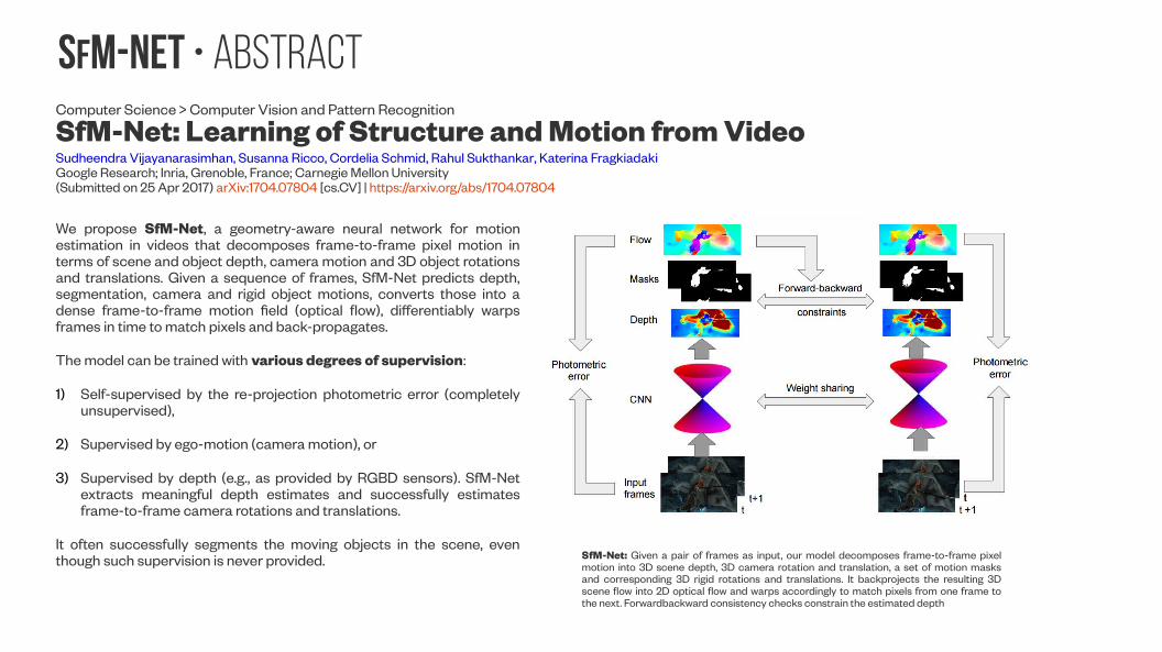
SfM-NeT • AbstractComputer Science > Computer Vision and Pattern Recognition

SfM-Net: Learning of Structure and Motion from VideoSudheendra Vijayanarasimhan, Susanna Ricco, Cordelia Schmid, Rahul Sukthankar, Katerina Fragkiadaki Google Research; Inria, Grenoble, France; Carnegie Mellon University(Submitted on 25 Apr 2017) arXiv:1704.07804 [cs.CV] | https://arxiv.org/abs/1704.07804

We propose SfM-Net, a geometry-aware neural network for motion estimation in videos that decomposes frame-to-frame pixel motion in terms of scene and object depth, camera motion and 3D object rotations and translations. Given a sequence of frames, SfM-Net predicts depth, segmentation, camera and rigid object motions, converts those into a dense frame-to-frame motion field (optical flow), differentiably warps frames in time to match pixels and back-propagates.

The model can be trained with various degrees of supervision:

1) Self-supervised by the re-projection photometric error (completely unsupervised),

2) Supervised by ego-motion (camera motion), or

3) Supervised by depth (e.g., as provided by RGBD sensors). SfM-Net extracts meaningful depth estimates and successfully estimates frame-to-frame camera rotations and translations.

It often successfully segments the moving objects in the scene, even though such supervision is never provided. SfM-Net: Given a pair of frames as input, our model decomposes frame-to-frame pixel

motion into 3D scene depth, 3D camera rotation and translation, a set of motion masks and corresponding 3D rigid rotations and translations. It backprojects the resulting 3D scene flow into 2D optical flow and warps accordingly to match pixels from one frame to the next. Forwardbackward consistency checks constrain the estimated depth

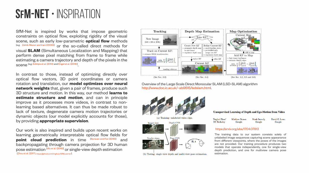
SfM-NeT • InspirationSfM-Net is inspired by works that impose geometric constraints on optical flow, exploiting rigidity of the visual scene, such as early low-parametric optical flow methods

[e.g. Zelnik-Manor and Irani (2000)] or the so-called direct methods for visual SLAM (Simultaneous Localization and Mapping) that perform dense pixel matching from frame to frame while estimating a camera trajectory and depth of the pixels in the scene [e.g. Schöps et al. (2014) and Engel et al. (2014)].

In contrast to those, instead of optimizing directly over optical flow vectors, 3D point coordinates or camera rotation and translation, our model optimizes over neural network weights that, given a pair of frames, produce such 3D structure and motion. In this way, our method learns to estimate structure and motion, and can in principle improve as it processes more videos, in contrast to non-learning based alternatives. It can thus be made robust to lack of texture, degenerate camera motion trajectories or dynamic objects (our model explicitly accounts for those), by providing appropriate supervision.

Our work is also inspired and builds upon recent works on learning geometrically interpretable optical flow fields for point cloud prediction in time [Byravan and Fox (2016)] and backpropagating through camera projection for 3D human pose estimation [Wu et al. (2016)] or single-view depth estimation [Zhou et al. (2017), https://github.com/tinghuiz/SfMLearner].

The training data to our system consists solely of unlabeled image sequences capturing scene appearance from different viewpoints, where the poses of the images are not provided. Our training procedure produces two models that operate independently, one for single-view depth prediction, and one for multiview camera pose estimation.

https://arxiv.org/abs/1704.07813

Overview of the Large Scale Direct Monocular SLAM (LSD-SLAM) algorithm http://www.doc.ic.ac.uk/~ab9515/lsdslam.html.

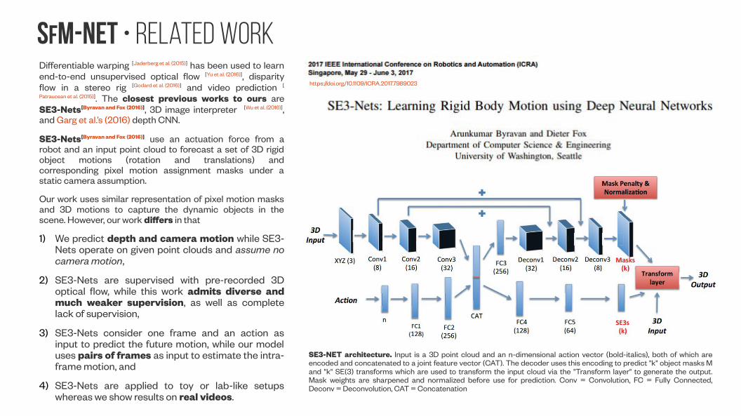
SfM-NeT • related WorkDifferentiable warping [Jaderberg et al. (2015)] has been used to learn end-to-end unsupervised optical flow [Yu et al. (2016)], disparity flow in a stereo rig [Godard et al. (2016)] and video prediction [

Patraucean et al. (2015)]. The closest previous works to ours are SE3-Nets[Byravan and Fox (2016)], 3D image interpreter [Wu et al. (2016)], and Garg et al.’s (2016) depth CNN.

SE3-Nets[Byravan and Fox (2016)] use an actuation force from a robot and an input point cloud to forecast a set of 3D rigid object motions (rotation and translations) and corresponding pixel motion assignment masks under a static camera assumption.

Our work uses similar representation of pixel motion masks and 3D motions to capture the dynamic objects in the scene. However, our work differs in that

1) We predict depth and camera motion while SE3-Nets operate on given point clouds and assume no camera motion,

2) SE3-Nets are supervised with pre-recorded 3D optical flow, while this work admits diverse and much weaker supervision, as well as complete lack of supervision,

3) SE3-Nets consider one frame and an action as input to predict the future motion, while our model uses pairs of frames as input to estimate the intra-frame motion, and

4) SE3-Nets are applied to toy or lab-like setups whereas we show results on real videos.

https://doi.org/10.1109/ICRA.2017.7989023

SE3-NET architecture. Input is a 3D point cloud and an n-dimensional action vector (bold-italics), both of which are encoded and concatenated to a joint feature vector (CAT). The decoder uses this encoding to predict "k" object masks M and "k" SE(3) transforms which are used to transform the input cloud via the "Transform layer" to generate the output. Mask weights are sharpened and normalized before use for prediction. Conv = Convolution, FC = Fully Connected, Deconv = Deconvolution, CAT = Concatenation

SfM-Net • Architecture

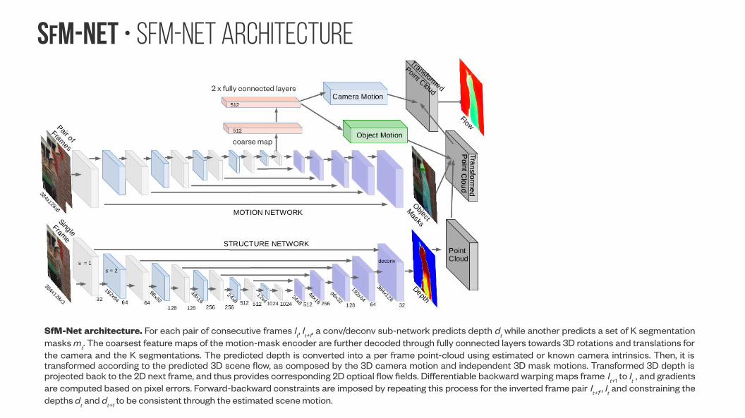
SfM-NeT • SfM-Net architecture

SfM-Net architecture. For each pair of consecutive frames It, I

t+1, a conv/deconv sub-network predicts depth d

t while another predicts a set of K segmentation

masks mt. The coarsest feature maps of the motion-mask encoder are further decoded through fully connected layers towards 3D rotations and translations for the camera and the K segmentations. The predicted depth is converted into a per frame point-cloud using estimated or known camera intrinsics. Then, it is transformed according to the predicted 3D scene flow, as composed by the 3D camera motion and independent 3D mask motions. Transformed 3D depth is projected back to the 2D next frame, and thus provides corresponding 2D optical flow fields. Differentiable backward warping maps frame It+1 to It , and gradients are computed based on pixel errors. Forward-backward constraints are imposed by repeating this process for the inverted frame pair It+1,, It and constraining the depths d

t and d

t+1 to be consistent through the estimated scene motion.

coarse map

2 x fully connected layers

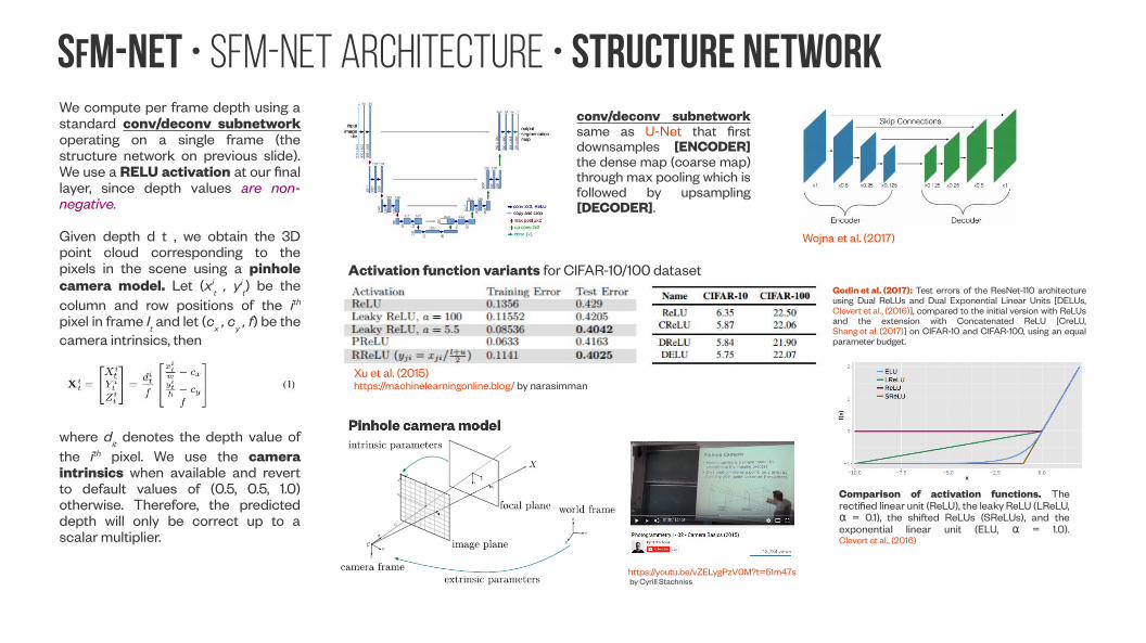
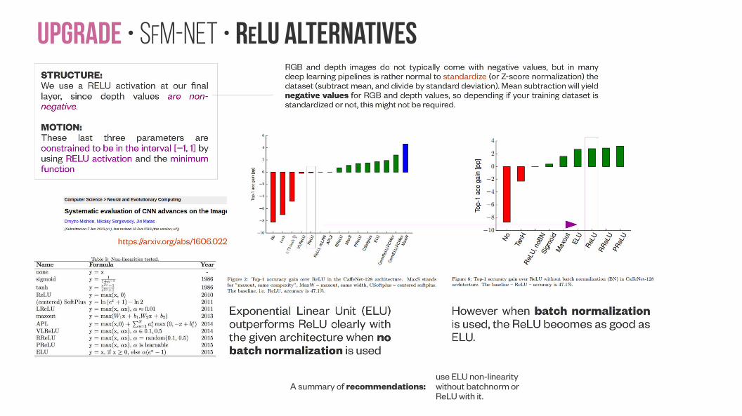
SfM-NeT • SfM-Net architecture • structure NetworkWe compute per frame depth using a standard conv/deconv subnetwork operating on a single frame (the structure network on previous slide). We use a RELU activation at our final layer, since depth values are non-negative.

Given depth d t , we obtain the 3D point cloud corresponding to the pixels in the scene using a pinhole camera model. Let (xi

t , yit) be the

column and row positions of the ith pixel in frame It and let (cx , cy , f) be the camera intrinsics, then

where dit denotes the depth value of

the ith pixel. We use the camera intrinsics when available and revert to default values of (0.5, 0.5, 1.0) otherwise. Therefore, the predicted depth will only be correct up to a scalar multiplier.

https://youtu.be/vZELygPzV0M?t=51m47s by Cyrill Stachniss

Xu et al. (2015)https://machinelearningonline.blog/ by narasimman

Activation function variants for CIFAR-10/100 datasetGodin et al. (2017): Test errors of the ResNet-110 architecture using Dual ReLUs and Dual Exponential Linear Units [DELUs, Clevert et al., (2016)], compared to the initial version with ReLUs and the extension with Concatenated ReLU [CreLU, Shang et al. (2017)] on CIFAR-10 and CIFAR-100, using an equal parameter budget.

Comparison of activation functions. The rectified linear unit (ReLU), the leaky ReLU (LReLU,

= 0.1), the shifted ReLUs (SReLUs), and the αexponential linear unit (ELU, = 1.0).αClevert et al., (2016)

conv/deconv subnetwork same as U-Net that first downsamples [ENCODER] the dense map (coarse map) through max pooling which is followed by upsampling [DECODER].

Wojna et al. (2017)

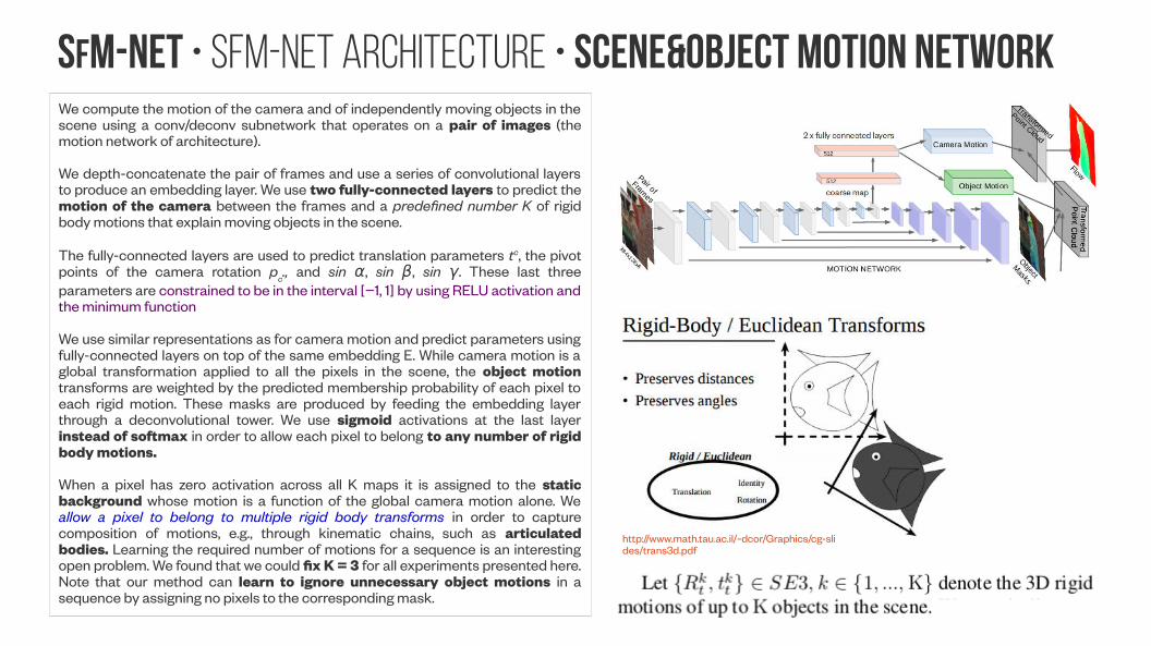
SfM-NeT • SfM-Net architecture • Scene&Object Motion NetworkWe compute the motion of the camera and of independently moving objects in the scene using a conv/deconv subnetwork that operates on a pair of images (the motion network of architecture).

We depth-concatenate the pair of frames and use a series of convolutional layers to produce an embedding layer. We use two fully-connected layers to predict the motion of the camera between the frames and a predefined number K of rigid body motions that explain moving objects in the scene.

The fully-connected layers are used to predict translation parameters tc, the pivot points of the camera rotation pc., and sin α, sin β, sin γ. These last three parameters are constrained to be in the interval [−1, 1] by using RELU activation and the minimum function

We use similar representations as for camera motion and predict parameters using fully-connected layers on top of the same embedding E. While camera motion is a global transformation applied to all the pixels in the scene, the object motion transforms are weighted by the predicted membership probability of each pixel to each rigid motion. These masks are produced by feeding the embedding layer through a deconvolutional tower. We use sigmoid activations at the last layer instead of softmax in order to allow each pixel to belong to any number of rigid body motions.

When a pixel has zero activation across all K maps it is assigned to the static background whose motion is a function of the global camera motion alone. We allow a pixel to belong to multiple rigid body transforms in order to capture composition of motions, e.g., through kinematic chains, such as articulated bodies. Learning the required number of motions for a sequence is an interesting open problem. We found that we could fix K = 3 for all experiments presented here. Note that our method can learn to ignore unnecessary object motions in a sequence by assigning no pixels to the corresponding mask.

http://www.math.tau.ac.il/~dcor/Graphics/cg-slides/trans3d.pdf

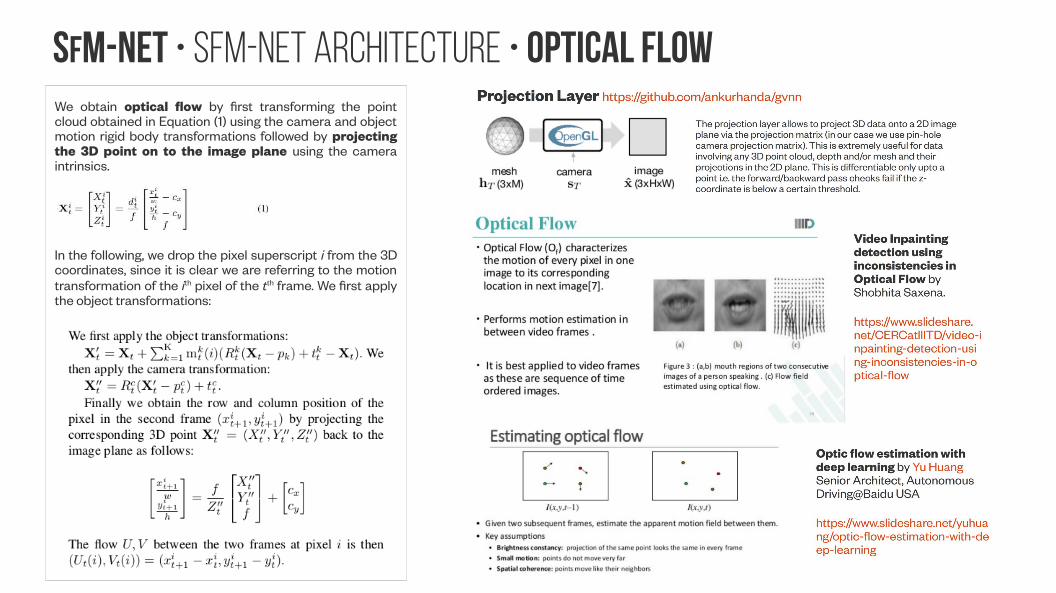
SfM-NeT • SfM-Net architecture • optical FlowWe obtain optical flow by first transforming the point cloud obtained in Equation (1) using the camera and object motion rigid body transformations followed by projecting the 3D point on to the image plane using the camera intrinsics.

In the following, we drop the pixel superscript i from the 3D coordinates, since it is clear we are referring to the motion transformation of the ith pixel of the tth frame. We first apply the object transformations:

Upgrade • SfM-NeT • Upgrade to architecture #1

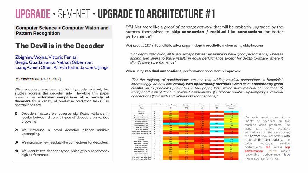
The Devil is in the DecoderZbigniew Wojna, Vittorio Ferrari, Sergio Guadarrama, Nathan Silberman, Liang-Chieh Chen, Alireza Fathi, Jasper Uijlings

While encoders have been studied rigorously, relatively few studies address the decoder side. Therefore this paper presents an extensive comparison of a variety of decoders for a variety of pixel-wise prediction tasks. Our contributions are:

1) Decoders matter: we observe significant variance in results between different types of decoders on various problems.

2) We introduce a novel decoder: bilinear additive upsampling.

3) We introduce new residual-like connections for decoders.

4) We identify two decoder types which give a consistently high performance.

SfM-Net more like a proof-of-concept network that will be probably upgraded by the authors themselves to skip-connection / residual-like connections for better performance?

Wojna et al. (2017) found little advantage in depth prediction when using skip layers:

“For depth prediction, all layers except bilinear upsampling have good performance, whereas adding skip layers to these results in equal performance except for depth-to-space, where it slightly lowers performance”

When using residual connections, performance consistently improves:

“For the majority of combinations, we see that adding residual connections is beneficial. Interestingly, we now can identify two upsampling methods which have consistently good results on all problems presented in this paper, both which have residual connections: (1) transposed convolutions + residual connections. (2) bilinear additive upsampling + residual connections (both with and without skip connections).”

Our main results comparing a variety of decoders on five machine vision problems. The upper part shows decoders without residual-like connections; the bottom shows decoders with residual-like connections. The colors represent relative performance: red means top performance, yellow means reasonable performance, blue means poor performance.

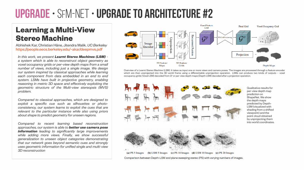
Upgrade • SfM-NeT • Upgrade to architecture #2Learning a Multi-View Stereo MachineAbhishek Kar, Christian Häne, Jitendra Malik. UC Berkeleyhttps://people.eecs.berkeley.edu/~akar/deepmvs.pdf

In this work, we present Learnt Stereo Machines (LSM) - a system which is able to reconstruct object geometry as voxel occupancy grids or per-view depth maps from a small number of views, including just a single image. We design our system inspired by classical approaches while learning each component from data embedded in an end to end system. LSMs have built in projective geometry, enabling reasoning in metric 3D space and effectively exploiting the geometric structure of the Multi-view stereopsis (MVS) problem.

Compared to classical approaches, which are designed to exploit a specific cue such as silhouettes or photo-consistency, our system learns to exploit the cues that are relevant to the particular instance while also using priors about shape to predict geometry for unseen regions.

Compared to recent learning based reconstruction approaches, our system is able to better use camera pose information leading to significantly large improvements while adding more views. Finally, we show successful generalization to unseen object categories demonstrating that our network goes beyond semantic cues and strongly uses geometric information for unified single and multi-view 3D reconstruction

Overview of a Learnt Stereo Machine (LSM). It takes as input one or more views and camera poses. The images are processed through a feature encoder which are then unprojected into the 3D world frame using a differentiable unprojection operation. LSMs can produce two kinds of outputs – voxel occupancy grids (Voxel LSM) decoded from Go or per-view depth maps (Depth LSM) decoded after a projection operation.

Qualitative results for per-view depth map prediction on ShapeNet. We show the depth maps predicted by Depth-LSM (visualized with shading from a shifted viewpoint) and the point cloud obtained by unprojecting them into world coordinates.

Upgrade • SfM-NeT • Relu alternatives

use ELU non-linearity without batchnorm or ReLU with it.

A summary of recommendations:

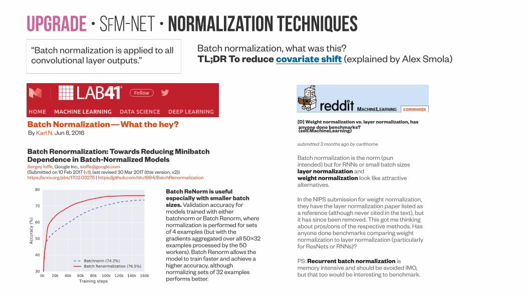
Upgrade • SfM-NeT • Normalization techniquesBatch normalization, what was this?TL;DR To reduce covariate shift (explained by Alex Smola)

[D] Weight normalization vs. layer normalization, has anyone done benchmarks? (self.MachineLearning)

submitted 3 months ago by carlthome

Batch normalization is the norm (pun intended) but for RNNs or small batch sizes layer normalization and weight normalization look like attractive alternatives.

In the NIPS submission for weight normalization, they have the layer normalization paper listed as a reference (although never cited in the text), but it has since been removed. This got me thinking about pros/cons of the respective methods. Has anyone done benchmarks comparing weight normalization to layer normalization (particularly for ResNets or RNNs)?

PS: Recurrent batch normalization is memory intensive and should be avoided IMO, but that too would be interesting to benchmark.

Batch Renormalization: Towards Reducing Minibatch Dependence in Batch-Normalized ModelsSergey Ioffe, Google Inc., sioffe@google.com(Submitted on 10 Feb 2017 (v1), last revised 30 Mar 2017 (this version, v2))https://arxiv.org/abs/1702.03275 | https://github.com/titu1994/BatchRenormalization

Batch Normalization — What the hey?By Karl N. Jun 8, 2016

Batch ReNorm is useful especially with smaller batch sizes. Validation accuracy for models trained with either batchnorm or Batch Renorm, where normalization is performed for sets of 4 examples (but with the gradients aggregated over all 50×32 examples processed by the 50 workers). Batch Renorm allows the model to train faster and achieve a higher accuracy, although normalizing sets of 32 examples performs better.

“Batch normalization is applied to all convolutional layer outputs.”

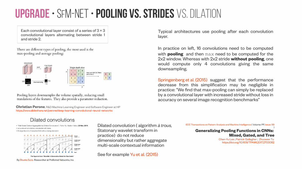
Upgrade • SfM-NeT • pooling vs. strides vs. dilation

Christian Perone, R&D Machine Learning Engineer and Software Engineer at HPhttps://www.slideshare.net/perone/deep-learning-convolutional-neural-networks

Typical architectures use pooling after each convolution layer.

In practice on left, 16 convolutions need to be computed with pooling and then max need to be computed for the 2x2 window. Whereas with 2x2 stride without pooling, one would compute only 4 convolutions giving the same downsampling.

Springenberg et al. (2015) suggest that the performance decrease from this simplification may be negligible in practice: “We find that max-pooling can simply be replaced by a convolutional layer with increased stride without loss in accuracy on several image recognition benchmarks”

Dilated convolution ( algorithm à trous, Statonary wavelet transform in practice) do not reduce dimensionality but rather aggregate multi-scale contextual information

See for example Yu et al. (2015)

IEEE Transactions on Pattern Analysis and Machine Intelligence ( Volume: PP, Issue: 99 )

Generalizing Pooling Functions in CNNs: Mixed, Gated, and Tree

Chen-Yu Lee ; Patrick Gallagher ; Zhuowen Tu https://doi.org/10.1109/TPAMI.2017.2703082

Each convolutional layer consist of a series of 3 × 3 convolutional layers alternating between stride 1 and stride 2.

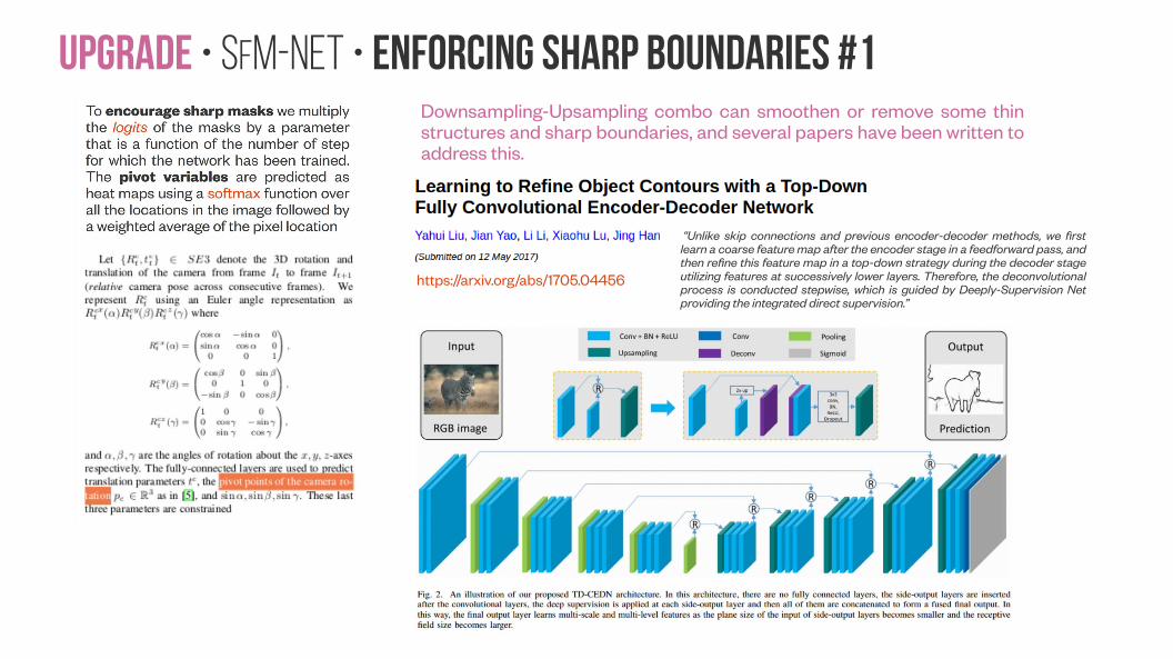
Upgrade • SfM-NeT • Enforcing sharp boundaries #1Downsampling-Upsampling combo can smoothen or remove some thin structures and sharp boundaries, and several papers have been written to address this.

“Unlike skip connections and previous encoder-decoder methods, we first learn a coarse feature map after the encoder stage in a feedforward pass, and then refine this feature map in a top-down strategy during the decoder stage utilizing features at successively lower layers. Therefore, the deconvolutional process is conducted stepwise, which is guided by Deeply-Supervision Net providing the integrated direct supervision.”

https://arxiv.org/abs/1705.04456

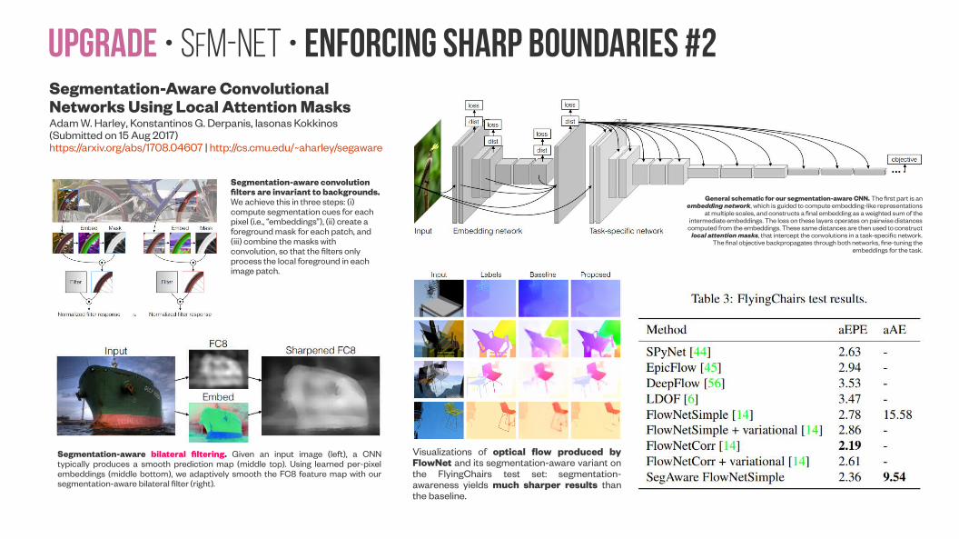
Upgrade • SfM-NeT • Enforcing sharp boundaries #2Segmentation-Aware Convolutional Networks Using Local Attention MasksAdam W. Harley, Konstantinos G. Derpanis, Iasonas Kokkinos(Submitted on 15 Aug 2017)https://arxiv.org/abs/1708.04607 | http://cs.cmu.edu/~aharley/segaware

Segmentation-aware convolution filters are invariant to backgrounds. We achieve this in three steps: (i) compute segmentation cues for each pixel (i.e., “embeddings”), (ii) create a foreground mask for each patch, and (iii) combine the masks with convolution, so that the filters only process the local foreground in each image patch.

Segmentation-aware bilateral filtering. Given an input image (left), a CNN typically produces a smooth prediction map (middle top). Using learned per-pixel embeddings (middle bottom), we adaptively smooth the FC8 feature map with our segmentation-aware bilateral filter (right).

General schematic for our segmentation-aware CNN. The first part is an embedding network, which is guided to compute embedding-like representations

at multiple scales, and constructs a final embedding as a weighted sum of the intermediate embeddings. The loss on these layers operates on pairwise distances

computed from the embeddings. These same distances are then used to construct local attention masks, that intercept the convolutions in a task-specific network.

The final objective backpropagates through both networks, fine-tuning the embeddings for the task.

Visualizations of optical flow produced by FlowNet and its segmentation-aware variant on the FlyingChairs test set: segmentation-awareness yields much sharper results than the baseline.

SfM-Net • Supervision

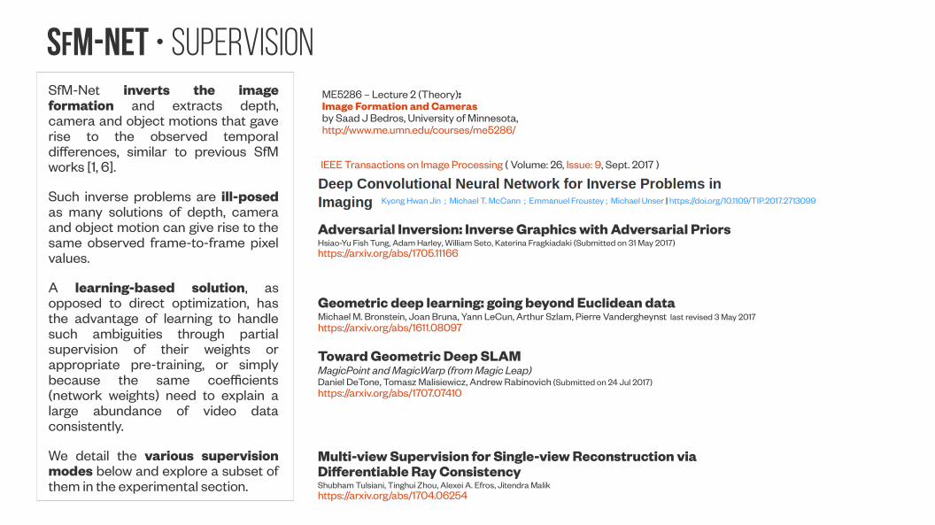
SfM-NeT • SupervisionSfM-Net inverts the image formation and extracts depth, camera and object motions that gave rise to the observed temporal differences, similar to previous SfM works [1, 6].

Such inverse problems are ill-posed as many solutions of depth, camera and object motion can give rise to the same observed frame-to-frame pixel values.

A learning-based solution, as opposed to direct optimization, has the advantage of learning to handle such ambiguities through partial supervision of their weights or appropriate pre-training, or simply because the same coefficients (network weights) need to explain a large abundance of video data consistently.

We detail the various supervision modes below and explore a subset of them in the experimental section.

Kyong Hwan Jin ; Michael T. McCann ; Emmanuel Froustey ; Michael Unser | https://doi.org/10.1109/TIP.2017.2713099

IEEE Transactions on Image Processing ( Volume: 26, Issue: 9, Sept. 2017 )

ME5286 – Lecture 2 (Theory): Image Formation and Camerasby Saad J Bedros, University of Minnesota, http://www.me.umn.edu/courses/me5286/

Adversarial Inversion: Inverse Graphics with Adversarial PriorsHsiao-Yu Fish Tung, Adam Harley, William Seto, Katerina Fragkiadaki (Submitted on 31 May 2017)https://arxiv.org/abs/1705.11166

Multi-view Supervision for Single-view Reconstruction via Differentiable Ray ConsistencyShubham Tulsiani, Tinghui Zhou, Alexei A. Efros, Jitendra Malikhttps://arxiv.org/abs/1704.06254

Toward Geometric Deep SLAMMagicPoint and MagicWarp (from Magic Leap)Daniel DeTone, Tomasz Malisiewicz, Andrew Rabinovich (Submitted on 24 Jul 2017)https://arxiv.org/abs/1707.07410

Geometric deep learning: going beyond Euclidean dataMichael M. Bronstein, Joan Bruna, Yann LeCun, Arthur Szlam, Pierre Vandergheynst last revised 3 May 2017https://arxiv.org/abs/1611.08097

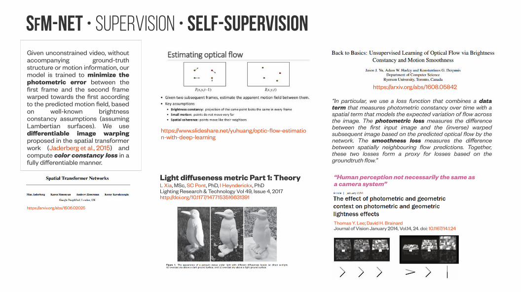
SfM-NeT • Supervision • Self-supervisionGiven unconstrained video, without accompanying ground-truth structure or motion information, our model is trained to minimize the photometric error between the first frame and the second frame warped towards the first according to the predicted motion field, based on well-known brightness constancy assumptions (assuming Lambertian surfaces). We use differentiable image warping proposed in the spatial transformer work (Jaderberg et al., 2015) and compute color constancy loss in a fully differentiable manner.

https://arxiv.org/abs/1608.05842

“In particular, we use a loss function that combines a data term that measures photometric constancy over time with a spatial term that models the expected variation of flow across the image. The photometric loss measures the difference between the first input image and the (inverse) warped subsequent image based on the predicted optical flow by the network. The smoothness loss measures the difference between spatially neighbouring flow predictions. Together, these two losses form a proxy for losses based on the groundtruth flow.”

https://www.slideshare.net/yuhuang/optic-flow-estimation-with-deep-learning

https://arxiv.org/abs/1506.02025

Light diffuseness metric Part 1: TheoryL Xia, MSc, SC Pont, PhD, I Heynderickx, PhDLighting Research & Technology Vol 49, Issue 4, 2017http://doi.org/10.1177/1477153516631391

Thomas Y. Lee; David H. Brainard Journal of Vision January 2014, Vol.14, 24. doi: 10.1167/14.1.24

“Human perception not necessarily the same as a camera system”

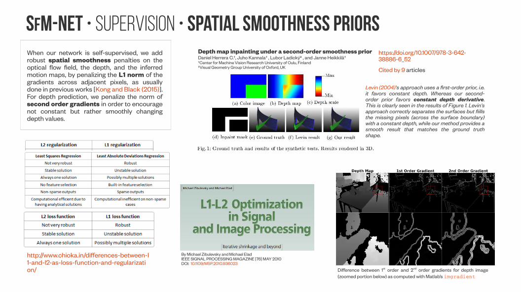
SfM-NeT • Supervision • Spatial smoothness priorsWhen our network is self-supervised, we add robust spatial smoothness penalties on the optical flow field, the depth, and the inferred motion maps, by penalizing the L1 norm of the gradients across adjacent pixels, as usually done in previous works [Kong and Black (2015)]. For depth prediction, we penalize the norm of second order gradients in order to encourage not constant but rather smoothly changing depth values.

http://www.chioka.in/differences-between-l1-and-l2-as-loss-function-and-regularization/

By Michael Zibulevsky and Michael EladIEEE SIGNAL PROCESSING MAGAZINE [76] MAY 2010DOI: 10.1109/MSP.2010.936023

Depth map inpainting under a second-order smoothness prior Daniel Herrera C.†, Juho Kannala† , Lubor Ladický‡ , and Janne Heikkilä† †Center for Machine Vision Research University of Oulu, Finland‡Visual Geometry Group University of Oxford, UK

Levin (2004)'s approach uses a first-order prior, i.e. it favors constant depth. Whereas our second-order prior favors constant depth derivative. This is clearly seen in the results of Figure 1. Levin's approach correctly separates the surfaces but fiills the missing pixels (across the surface boundary) with a constant depth, while our method provides a smooth result that matches the ground truth shape.

Difference between 1st order and 2nd order gradients for depth image (zoomed portion below) as computed with Matlab’s imgradient

https://doi.org/10.1007/978-3-642-38886-6_52

Cited by 9 articles

SfM-NeT • Supervision • Forward-backward consistency constraintsWe incorporate forward-backward consistency constraints between inferred scene depth in different frames. Composing scene flow forward and backward across consecutive frames allows us to impose such forward-backward consistency cycles across more than one frame gaps, however, we have not yet seen empirical gain from doing so.

In other words one could “robustify” the network by having more temporal samples which should improve inlier / outlier separation

Science of Electrical Engineering (ICSEE), IEEE International Conference on theA Depth Restoration Occlusionless Temporal DatasetDaniel Rotman ; Guy Gilboa Electrical Engineering Department, Technion - Israel Institute of Technology.https://doi.org/10.1109/3DV.2016.26

“Utilizing multiple frames, we create a number of possibilities for an initial degraded depth map, which allows us to arrive at a more educated decision when refining depth images. Evaluating this method with our dataset shows significant benefits, particularly for overcoming real sensor-noise artifacts.”

The dataset is freely downloadable at: http://visl.technion.ac.il/databases/drot2016/

3D Vision (3DV), 2016 Fourth International Conference on, 16-18 Nov. 2016Frame rate reduction of depth cameras by RGB-based depth predictionDaniel Rotman ; Omer Cohen ; Guy Gilboa Electrical Engineering Department, Technion - Israel Institute of Technology.https://doi.org/10.1109/ICSEE.2016.7806153

“Depth cameras are becoming widely used for facilitating fast and robust natural user interaction. But measuring depth can be high in power consumption mainly due to the active infrared illumination involved in the acquisition process, for both structured-light and time-of-flight technologies. It becomes a critical issue when the sensors are mounted on hand-held (mobile) devices, where power usage is of the essence. A method is proposed to reduce the depth acquisition frame rate, possibly by factors of 2 or 3, thus saving considerable power.

The compensation is done by calculating reliable depth estimations using a coupled color (RGB) camera working at full frame rate. These predictions, which are shown to perform outstandingly, create for the end user or application the perception of a depth sensor working at full frame rate. Quality measures based on skeleton extraction and depth inaccuracy are used to calculate the deviation from the ground truth.”

SfM-NeT • Supervision • Supervising depthIf depth is available on parts of the input image, such as with video sequences captured by a Kinect sensor, we can use depth supervision in the form of robust depth regression.

No in theory we can give targets automatically for SfM pipeline designed to operate:

1) without depth sensor, such as traditional smartphone

- Target with Kinect or high-quality laser scanner

2) Google Tango smartphone with “low-quality depth sensing”

- Target with high-quality laser scanner

No need for massive Mechanic Turker workforce for boring time-consuming labeling

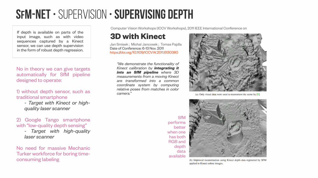
3D with Kinect Computer Vision Workshops (ICCV Workshops), 2011 IEEE International Conference on

Jan Smisek ; Michal Jancosek ; Tomas PajdlaDate of Conference: 6-13 Nov. 2011https://doi.org/10.1109/ICCVW.2011.6130380

“We demonstrate the functionality of Kinect calibration by integrating it into an SfM pipeline where 3D measurements from a moving Kinect are transformed into a common coordinate system by computing relative poses from matches in color camera.”

SfM performs

better when one has both RGB and

depth data

available

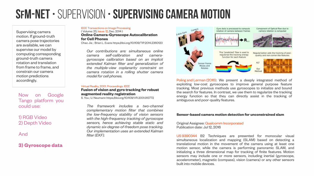
SfM-NeT • Supervision • Supervising camera motionSupervising camera motion. If ground-truth camera pose trajectories are available, we can supervise our model by computing corresponding ground-truth camera rotation and translation from frame to frame, and constrain our camera motion predictions accordingly.

IEEE Transactions on Image Processing ( Volume: 23, Issue: 12, Dec. 2014 )Online Camera-Gyroscope Autocalibration for Cell PhonesChao Jia ; Brian L. Evans https://doi.org/10.1109/TIP.2014.2360120

Our contributions are: simultaneous online camera self-calibration and camera-gyroscope calibration based on an implicit extended Kalman filter and generalization of the multiple-view coplanarity constraint on camera rotation in a rolling shutter camera model for cell phones.

Now on Google Tango platform you could use:

1) RGB Video2) Depth Video

And

3) Gyroscope data

Sensor-based camera motion detection for unconstrained slam

Original Assignee: Qualcomm IncorporatedPublication date: Jul 12, 2016

US 9390344 B2 Techniques are presented for monocular visual simultaneous localization and mapping (SLAM) based on detecting a translational motion in the movement of the camera using at least one motion sensor, while the camera is performing panoramic SLAM, and initializing a three dimensional map for tracking of finite features. Motion sensors may include one or more sensors, including inertial (gyroscope, accelerometer), magnetic (compass), vision (camera) or any other sensors built into mobile devices.

Virtual Reality, 2001. Proceedings. IEEEFusion of vision and gyro tracking for robust augmented reality registrationS. You ; U. Neumann https://doi.org/10.1109/VR.2001.913772

The framework includes a two-channel complementary motion filter that combines the low-frequency stability of vision sensors with the high-frequency tracking of gyroscope sensors, hence achieving stable static and dynamic six-degree-of-freedom pose tracking. Our implementation uses an extended Kalman filter (EKF).

Poling and Lerman (2016): We present a deeply integrated method of exploiting low-cost gyroscopes to improve general purpose feature tracking. Most previous methods use gyroscopes to initialize and bound the search for features. In contrast, we use them to regularize the tracking energy function so that they can directly assist in the tracking of ambiguous and poor-quality features.

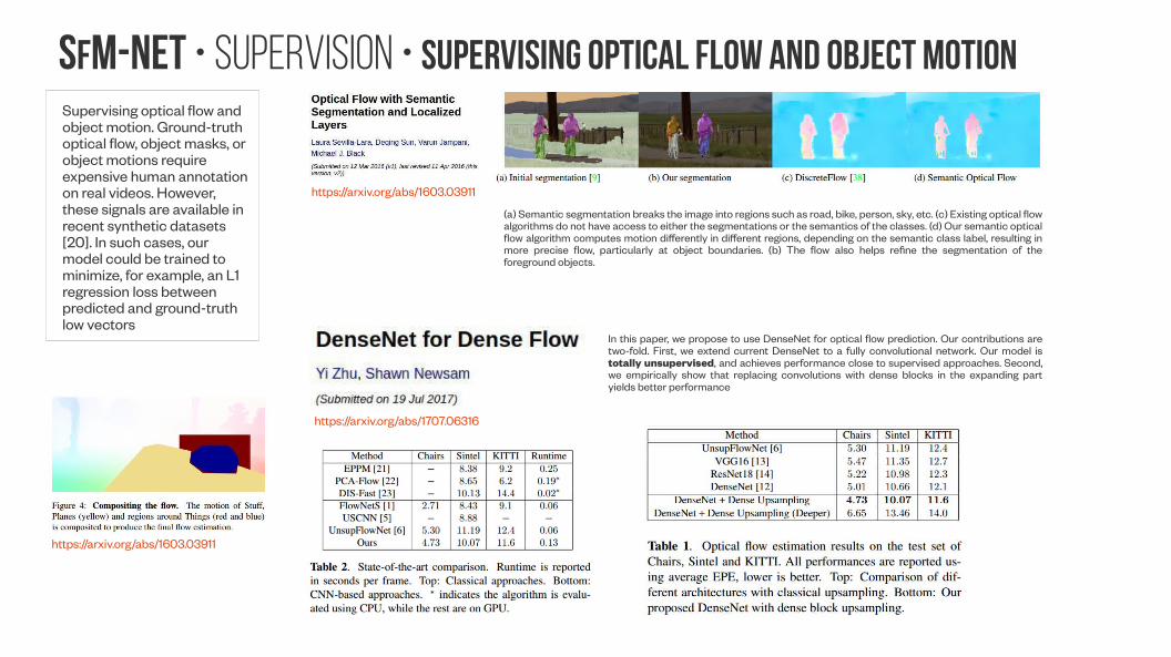
SfM-NeT • Supervision • Supervising optical flow and object motionSupervising optical flow and object motion. Ground-truth optical flow, object masks, or object motions require expensive human annotation on real videos. However, these signals are available in recent synthetic datasets [20]. In such cases, our model could be trained to minimize, for example, an L1 regression loss between predicted and ground-truth low vectors

https://arxiv.org/abs/1707.06316

In this paper, we propose to use DenseNet for optical flow prediction. Our contributions are two-fold. First, we extend current DenseNet to a fully convolutional network. Our model is totally unsupervised, and achieves performance close to supervised approaches. Second, we empirically show that replacing convolutions with dense blocks in the expanding part yields better performance

https://arxiv.org/abs/1603.03911

(a) Semantic segmentation breaks the image into regions such as road, bike, person, sky, etc. (c) Existing optical flow algorithms do not have access to either the segmentations or the semantics of the classes. (d) Our semantic optical flow algorithm computes motion differently in different regions, depending on the semantic class label, resulting in more precise flow, particularly at object boundaries. (b) The flow also helps refine the segmentation of the foreground objects.

https://arxiv.org/abs/1603.03911

Upgrade • Supervision • Loss Function #1

http://doi.ieeecomputersociety.org/10.1109/TPAMI.2007.1171

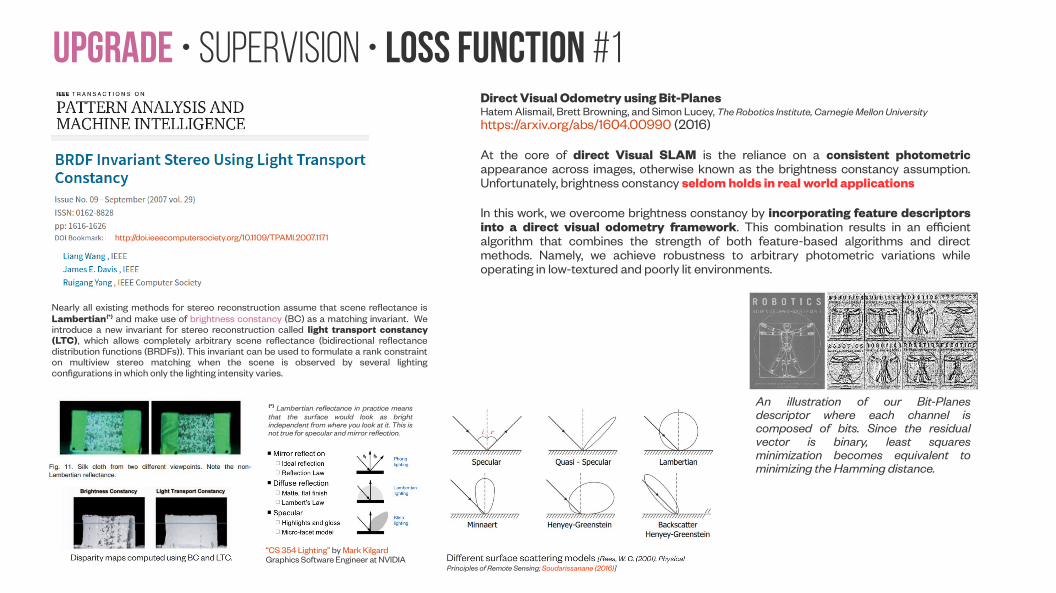
Nearly all existing methods for stereo reconstruction assume that scene reflectance is Lambertian{*} and make use of brightness constancy (BC) as a matching invariant. We introduce a new invariant for stereo reconstruction called light transport constancy (LTC), which allows completely arbitrary scene reflectance (bidirectional reflectance distribution functions (BRDFs)). This invariant can be used to formulate a rank constraint on multiview stereo matching when the scene is observed by several lighting configurations in which only the lighting intensity varies.

{*} Lambertian reflectance in practice means that the surface would look as bright independent from where you look at it. This is not true for specular and mirror reflection.

“CS 354 Lighting” by Mark KilgardGraphics Software Engineer at NVIDIA

Direct Visual Odometry using Bit-PlanesHatem Alismail, Brett Browning, and Simon Lucey, The Robotics Institute, Carnegie Mellon Universityhttps://arxiv.org/abs/1604.00990 (2016)

At the core of direct Visual SLAM is the reliance on a consistent photometric appearance across images, otherwise known as the brightness constancy assumption. Unfortunately, brightness constancy seldom holds in real world applications

In this work, we overcome brightness constancy by incorporating feature descriptors into a direct visual odometry framework. This combination results in an efficient algorithm that combines the strength of both feature-based algorithms and direct methods. Namely, we achieve robustness to arbitrary photometric variations while operating in low-textured and poorly lit environments.

An illustration of our Bit-Planes descriptor where each channel is composed of bits. Since the residual vector is binary, least squares minimization becomes equivalent to minimizing the Hamming distance.

Principles of Remote Sensing; Soudarissanane (2016)]

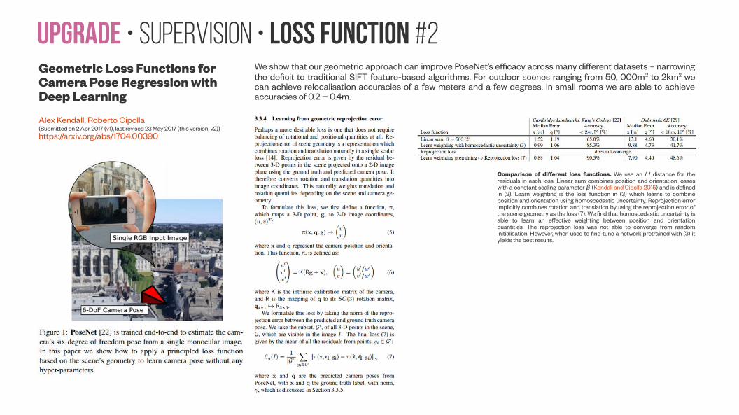
Upgrade • Supervision • Loss Function #2Geometric Loss Functions for Camera Pose Regression with Deep Learning

Alex Kendall, Roberto Cipolla(Submitted on 2 Apr 2017 (v1), last revised 23 May 2017 (this version, v2))https://arxiv.org/abs/1704.00390

We show that our geometric approach can improve PoseNet’s efficacy across many different datasets – narrowing the deficit to traditional SIFT feature-based algorithms. For outdoor scenes ranging from 50, 000m2 to 2km2 we can achieve relocalisation accuracies of a few meters and a few degrees. In small rooms we are able to achieve accuracies of 0.2 − 0.4m.

Comparison of different loss functions. We use an L1 distance for the residuals in each loss. Linear sum combines position and orientation losses with a constant scaling parameter β (Kendall and Cipolla 2015) and is defined in (2). Learn weighting is the loss function in (3) which learns to combine position and orientation using homoscedastic uncertainty. Reprojection error implicitly combines rotation and translation by using the reprojection error of the scene geometry as the loss (7). We find that homoscedastic uncertainty is able to learn an effective weighting between position and orientation quantities. The reprojection loss was not able to converge from random initialisation. However, when used to fine-tune a network pretrained with (3) it yields the best results.

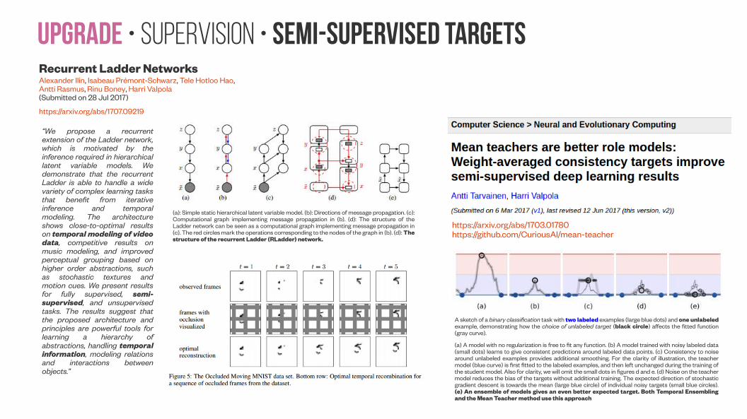
Upgrade • Supervision • Semi-supervised targetsRecurrent Ladder NetworksAlexander Ilin, Isabeau Prémont-Schwarz, Tele Hotloo Hao, Antti Rasmus, Rinu Boney, Harri Valpola(Submitted on 28 Jul 2017)

https://arxiv.org/abs/1707.09219

“We propose a recurrent extension of the Ladder network, which is motivated by the inference required in hierarchical latent variable models. We demonstrate that the recurrent Ladder is able to handle a wide variety of complex learning tasks that benefit from iterative inference and temporal modeling. The architecture shows close-to-optimal results on temporal modeling of video data, competitive results on music modeling, and improved perceptual grouping based on higher order abstractions, such as stochastic textures and motion cues. We present results for fully supervised, semi-supervised, and unsupervised tasks. The results suggest that the proposed architecture and principles are powerful tools for learning a hierarchy of abstractions, handling temporal information, modeling relations and interactions between objects.”

(a): Simple static hierarchical latent variable model. (b): Directions of message propagation. (c): Computational graph implementing message propagation in (b). (d): The structure of the Ladder network can be seen as a computational graph implementing message propagation in (c). The red circles mark the operations corresponding to the nodes of the graph in (b). (d): The structure of the recurrent Ladder (RLadder) network.

https://arxiv.org/abs/1703.01780https://github.com/CuriousAI/mean-teacher

A sketch of a binary classification task with two labeled examples (large blue dots) and one unlabeled example, demonstrating how the choice of unlabeled target (black circle) affects the fitted function (gray curve).

(a) A model with no regularization is free to fit any function. (b) A model trained with noisy labeled data (small dots) learns to give consistent predictions around labeled data points. (c) Consistency to noise around unlabeled examples provides additional smoothing. For the clarity of illustration, the teacher model (blue curve) is first fitted to the labeled examples, and then left unchanged during the training of the student model. Also for clarity, we will omit the small dots in figures d and e. (d) Noise on the teacher model reduces the bias of the targets without additional training. The expected direction of stochastic gradient descent is towards the mean (large blue circle) of individual noisy targets (small blue circles). (e) An ensemble of models gives an even better expected target. Both Temporal Ensembling and the Mean Teacher method use this approach

Upgrade • Supervision • “proxy” supervised targets

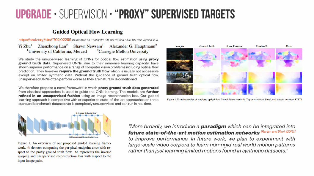
https://arxiv.org/abs/1702.02295 (Submitted on 8 Feb 2017 (v1), last revised 1 Jul 2017 (this version, v2))

We study the unsupervised learning of CNNs for optical flow estimation using proxy ground truth data. Supervised CNNs, due to their immense learning capacity, have shown superior performance on a range of computer vision problems including optical flow prediction. They however require the ground truth flow which is usually not accessible except on limited synthetic data. Without the guidance of ground truth optical flow, unsupervised CNNs often perform worse as they are naturally ill-conditioned.

We therefore propose a novel framework in which proxy ground truth data generated from classical approaches is used to guide the CNN learning. The models are further refined in an unsupervised fashion using an image reconstruction loss. Our guided learning approach is competitive with or superior to state-of-the-art approaches on three standard benchmark datasets yet is completely unsupervised and can run in real time.

“More broadly, we introduce a paradigm which can be integrated into future state-of-the-art motion estimation networks [Ranjan and Black (2016)] to improve performance. In future work, we plan to experiment with large-scale video corpora to learn non-rigid real world motion patterns rather than just learning limited motions found in synthetic datasets.”

Upgrade • Supervision • Self-supervision

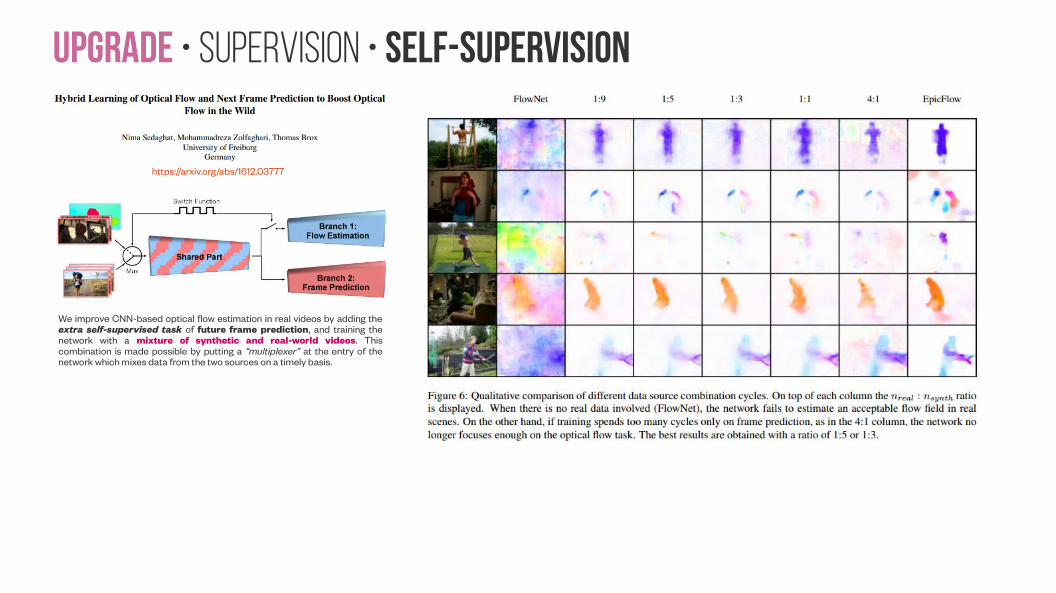
https://arxiv.org/abs/1612.03777

We improve CNN-based optical flow estimation in real videos by adding the extra self-supervised task of future frame prediction, and training the network with a mixture of synthetic and real-world videos. This combination is made possible by putting a “multiplexer” at the entry of the network which mixes data from the two sources on a timely basis.

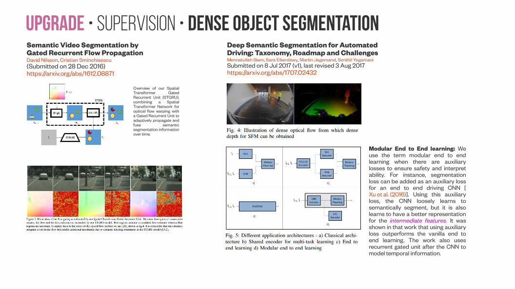
Upgrade • Supervision • Dense object segmentationSemantic Video Segmentation by Gated Recurrent Flow PropagationDavid Nilsson, Cristian Sminchisescu(Submitted on 28 Dec 2016)https://arxiv.org/abs/1612.08871

Deep Semantic Segmentation for Automated Driving: Taxonomy, Roadmap and ChallengesMennatullah Siam, Sara Elkerdawy, Martin Jagersand, Senthil YogamaniSubmitted on 8 Jul 2017 (v1), last revised 3 Aug 2017https://arxiv.org/abs/1707.02432

Overview of our Spatial Transformer Gated Recurrent Unit (STGRU), combining a Spatial Transformer Network for optical flow warping with a Gated Recurrent Unit to adaptively propagate and fuse semantic segmentation information over time.

Modular End to End learning: We use the term modular end to end learning when there are auxiliary losses to ensure safety and interpret ability. For instance, segmentation loss can be added as an auxiliary loss for an end to end driving CNN [Xu et al. (2016)]. Using this auxiliary loss, the CNN loosely learns to semantically segment, but it is also learns to have a better representation for the intermediate features. It was shown in that work that using auxiliary loss outperforms the vanilla end to end learning. The work also uses recurrent gated unit after the CNN to model temporal information.

Upgrade • Supervision • generative motion and content

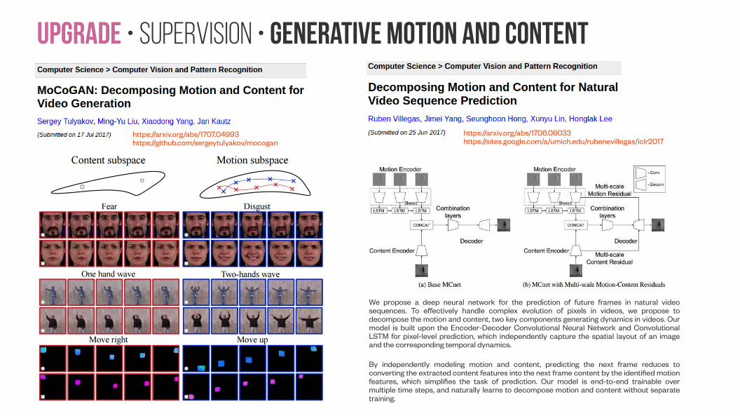
https://arxiv.org/abs/1707.04993https://github.com/sergeytulyakov/mocogan

https://arxiv.org/abs/1706.08033https://sites.google.com/a/umich.edu/rubenevillegas/iclr2017

We propose a deep neural network for the prediction of future frames in natural video sequences. To effectively handle complex evolution of pixels in videos, we propose to decompose the motion and content, two key components generating dynamics in videos. Our model is built upon the Encoder-Decoder Convolutional Neural Network and Convolutional LSTM for pixel-level prediction, which independently capture the spatial layout of an image and the corresponding temporal dynamics.

By independently modeling motion and content, predicting the next frame reduces to converting the extracted content features into the next frame content by the identified motion features, which simplifies the task of prediction. Our model is end-to-end trainable over multiple time steps, and naturally learns to decompose motion and content without separate training.

Upgrade • Supervision • data Augmentation

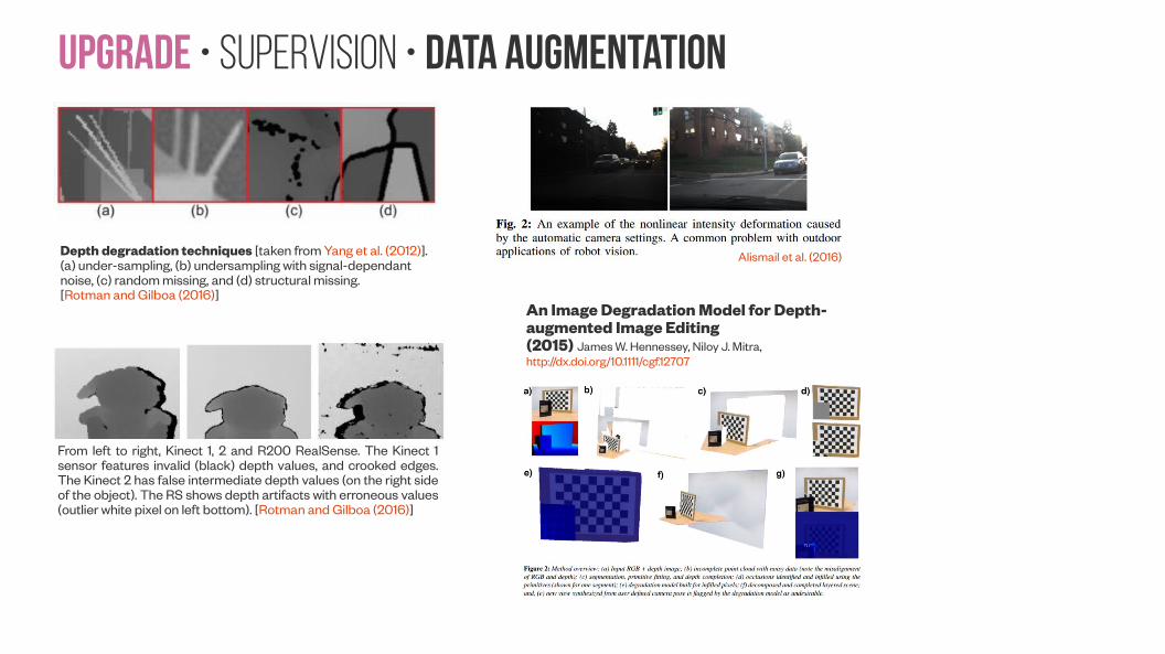
Depth degradation techniques [taken from Yang et al. (2012)]. (a) under-sampling, (b) undersampling with signal-dependant noise, (c) random missing, and (d) structural missing. [Rotman and Gilboa (2016)]

From left to right, Kinect 1, 2 and R200 RealSense. The Kinect 1 sensor features invalid (black) depth values, and crooked edges. The Kinect 2 has false intermediate depth values (on the right side of the object). The RS shows depth artifacts with erroneous values (outlier white pixel on left bottom). [Rotman and Gilboa (2016)]

Alismail et al. (2016)

An Image Degradation Model for Depth-augmented Image Editing(2015) James W. Hennessey, Niloy J. Mitra, http://dx.doi.org/10.1111/cgf.12707

Upgrade • Supervision • (multimodal) decomposition

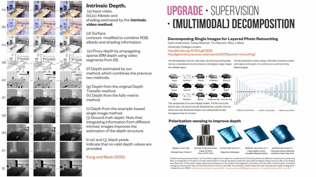
Intrinsic Depth. (a) Input video. (b),(c) Albedo andshading estimated by the intrinsic video method.

(d) Surfacecontours modified to combine RGB, albedo and shading information.

(e) Proxy depth by propagating sparse SfM depth using video segments from [9].

(f) Depth estimated by ourmethod, which combines the previous two methods.

(g) Depth from the original Depth Transfer method.(h) Depth from the fully-metric method.

(i) Depth from the example-basedsingle image method.(j) Ground truth depth. Note that integrating information from different intrinsic images improves the estimation of the depth structure.

In (e) and (j), black pixelsindicate that no valid depth values are provided.

Kong and Black (2015)

Decomposing Single Images for Layered Photo RetouchingCarlo Innamorati, Tobias Ritschel. Tim Weyrich. Niloy J. MitraUniversity College London http://dx.doi.org/10.1111/cgf.13220http://geometry.cs.ucl.ac.uk/projects/2017/layered-retouching/

Outline of proposed technique. (a) The Kinect depth of an object is combined with (b) three photos at different rotations of a polarizing filter. (c) Integration of surface normals obtained from Fresnel equations. Note the azimuthal ambiguity (observed as a flip in the shape) and distortion of the zenith angle (observed as flatness in the shape). (d) Integration of surface normals after correcting for azimuthal ambiguity removes the flip, and the final result is shown in (e) after correcting for zenith distortion and using physics-based integration. Kadambi et al. (2015) - http://web.media.mit.edu/~achoo/polar3D/ - http://news.mit.edu/2015/algorithms-boost-3-d-imaging-resolution-1000-times-1201

Polarization-sensing to improve depth

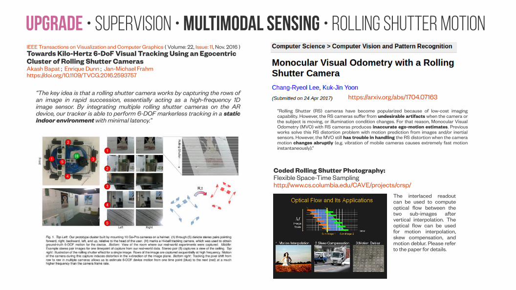
Upgrade • Supervision • Multimodal Sensing • Rolling shutter motionIEEE Transactions on Visualization and Computer Graphics ( Volume: 22, Issue: 11, Nov. 2016 )Towards Kilo-Hertz 6-DoF Visual Tracking Using an Egocentric Cluster of Rolling Shutter CamerasAkash Bapat ; Enrique Dunn ; Jan-Michael Frahmhttps://doi.org/10.1109/TVCG.2016.2593757

“The key idea is that a rolling shutter camera works by capturing the rows of an image in rapid succession, essentially acting as a high-frequency 1D image sensor. By integrating multiple rolling shutter cameras on the AR device, our tracker is able to perform 6-DOF markerless tracking in a static indoor environment with minimal latency.”

https://arxiv.org/abs/1704.07163

“Rolling Shutter (RS) cameras have become popularized because of low-cost imaging capability. However, the RS cameras suffer from undesirable artifacts when the camera or the subject is moving, or illumination condition changes. For that reason, Monocular Visual Odometry (MVO) with RS cameras produces inaccurate ego-motion estimates. Previous works solve this RS distortion problem with motion prediction from images and/or inertial sensors. However, the MVO still has trouble in handling the RS distortion when the camera motion changes abruptly (e.g. vibration of mobile cameras causes extremely fast motion instantaneously).”

Coded Rolling Shutter Photography:Flexible Space-Time Samplinghttp://www.cs.columbia.edu/CAVE/projects/crsp/

The interlaced readout can be used to compute optical flow between the two sub-images after vertical interpolation. The optical flow can be used for motion interpolation, skew compensation, and motion deblur. Please refer to the paper for details.

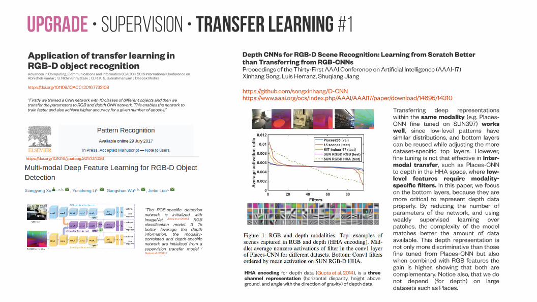
Upgrade • Supervision • Transfer learning #1Application of transfer learning in RGB-D object recognitionAdvances in Computing, Communications and Informatics (ICACCI), 2016 International Conference onAbhishek Kumar ; S. Nithin Shrivatsav ; G. R. K. S. Subrahmanyam ; Deepak Mishra

https://doi.org/10.1109/ICACCI.2016.7732108

“Firstly we trained a CNN network with 10 classes of different objects and then we transfer the parameters to RGB and depth CNN network. This enables the network to train faster and also achieve higher accuracy for a given number of epochs.”

Depth CNNs for RGB-D Scene Recognition: Learning from Scratch Better than Transferring from RGB-CNNs Proceedings of the Thirty-First AAAI Conference on Artificial Intelligence (AAAI-17)Xinhang Song, Luis Herranz, Shuqiang Jiang

https://github.com/songxinhang/D-CNNhttps://www.aaai.org/ocs/index.php/AAAI/AAAI17/paper/download/14695/14310

HHA encoding for depth data (Gupta et al. 2014), is a three channel representation (horizontal disparity, height above ground, and angle with the direction of gravity) of depth data.

Transferring deep representations within the same modality (e.g. Places-CNN fine tuned on SUN397) works well, since low-level patterns have similar distributions, and bottom layers can be reused while adjusting the more dataset-specific top layers. However, fine tuning is not that effective in inter-modal transfer, such as Places-CNN to depth in the HHA space, where low-level features require modality-specific filters. In this paper, we focus on the bottom layers, because they are more critical to represent depth data properly. By reducing the number of parameters of the network, and using weakly supervised learning over patches, the complexity of the model matches better the amount of data available. This depth representation is not only more discriminative than those fine tuned from Places-CNN but also when combined with RGB features the gain is higher, showing that both are complementary. Notice also, that we do not depend (for depth) on large datasets such as Places.

https://doi.org/10.1016/j.patcog.2017.07.026

“The RGB-specific detection network is initialized with ImageNet [Deng et al. (2009)] RGB classification model. 3 To better leverage the depth information, the modality-correlated and depth-specific network are initialized from a supervision transfer model [

Gupta et al. (2016)]”

Upgrade • Supervision • Transfer learning #2Learning Transferrable Knowledge for Semantic Segmentation With Deep Convolutional Neural Network

Seunghoon Hong, Junhyuk Oh, Honglak Lee, Bohyung Han; The IEEE Conference on Computer Vision and Pattern Recognition (CVPR), 2016, pp. 3204-3212https://doi.org/10.1109/CVPR.2016.349

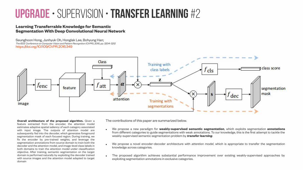
Overall architecture of the proposed algorithm. Given a feature extracted from the encoder, the attention model estimates adaptive spatial saliency of each category associated with input image. The outputs of attention model are subsequently fed into the decoder, which generates foreground segmentation mask of each focused region. During training, we fix the encoder by pre-trained weights, and leverage the segmentation annotations from source domain to train both the decoder and the attention model, and image-level class labels in both domains to train the attention model under classification objective. After training, semantic segmentation on the target domain is performed naturally by exploiting the decoder trained with source images and the attention model adapted to target domain

The contributions of this paper are summarized below.

● We propose a new paradigm for weakly-supervised semantic segmentation, which exploits segmentation annotations from different categories to guide segmentations with weak annotations. To our knowledge, this is the first attempt to tackle the weakly-supervised semantic segmentation problem by transfer learning.

● We propose a novel encoder-decoder architecture with attention model, which is appropriate to transfer the segmentation knowledge across categories.

● The proposed algorithm achieves substantial performance improvement over existing weakly-supervised approaches by exploiting segmentation annotations in exclusive categories.

Upgrade • Supervision • Transfer learning #3Borrowing Treasures from the Wealthy: Deep Transfer Learning through Selective Joint Fine-tuningWeifeng Ge, Yizhou Yu (Submitted on 28 Feb 2017 (v1), last revised 6 Jun 2017 (this version, v2))https://arxiv.org/abs/1702.08690https://github.com/ZYYSzj/Selective-Joint-Fine-tuning

In this paper, we introduce a source-target selective joint fine-tuning scheme for improving the performance of deep learning tasks with insufficient training data. In this scheme, a target learning task with insufficient training data is carried out simultaneously with another source learning task with abundant training data. However, the source learning task does not use all existing training data. Our core idea is to identify and use a subset of training images from the original source learning task whose low-level characteristics are similar to those from the target learning task, and jointly fine-tune shared convolutional layers for both tasks.

Pipeline of the proposed selective joint fine-tuning. From left to right: (a) Datasets in the source domain and the target domain. (b) Select nearest neighbors of each target domain training sample in the source domain via a low-level feature space. (c) Deep convolutional neural network initialized with weights pre-trained on ImageNet or Places. (d) Jointly optimize the source and target cost functions in their own label spaces.

Similar Image Search

There is a unique step in our pipeline. For each image from the target domain, we search a certain number of images with similar low-level characteristics from the source domain. Only images returned from these searches are used as training images for the source learning task in selective joint fine-tuning. We elaborate this image search step below.

In summary, this paper has the following contributions:

● We introduce a new deep transfer learning scheme, called selective joint fine-tuning, for improving the performance of deep learning tasks with insufficient training data. It is an important step forward in the context of the widely adopted strategy of fine-tuning a pre-trained deep neural network.

● We develop a novel pipeline for implementing this deep transfer learning scheme. Specifically, we compute descriptors from linear or nonlinear filter bank responses on training images from both tasks, and use such descriptors to search for a desired subset of training samples for the source learning task.

● Experiments demonstrate that our deep transfer learning scheme achieves state-of-the-art performance on multiple visual classification tasks with insufficient training data for deep learning.

SfM-Net • Implementation

SfM-NeT • implementation Details

coarse map

2 x fully connected layers

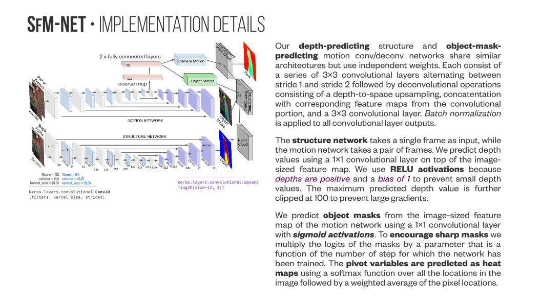
Our depth-predicting structure and object-mask-predicting motion conv/deconv networks share similar architectures but use independent weights. Each consist of a series of 3×3 convolutional layers alternating between stride 1 and stride 2 followed by deconvolutional operations consisting of a depth-to-space upsampling, concatentation with corresponding feature maps from the convolutional portion, and a 3×3 convolutional layer. Batch normalization is applied to all convolutional layer outputs.

The structure network takes a single frame as input, while the motion network takes a pair of frames. We predict depth values using a 1×1 convolutional layer on top of the image-sized feature map. We use RELU activations because depths are positive and a bias of 1 to prevent small depth values. The maximum predicted depth value is further clipped at 100 to prevent large gradients.

We predict object masks from the image-sized feature map of the motion network using a 1×1 convolutional layer with sigmoid activations. To encourage sharp masks we multiply the logits of the masks by a parameter that is a function of the number of step for which the network has been trained. The pivot variables are predicted as heat maps using a softmax function over all the locations in the image followed by a weighted average of the pixel locations.

keras.layers.convolutional.Conv2D(filters, kernel_size, strides)

filters = 32strides = (1,1)

kernel_size = (3,3)

filters = 64strides = (2,2)kernel_size = (3,3) keras.layers.convolutional.UpSamp

ling2D(size=(2, 2))

SfM-Net • Results

SfM-NeT • Experimental Results #1

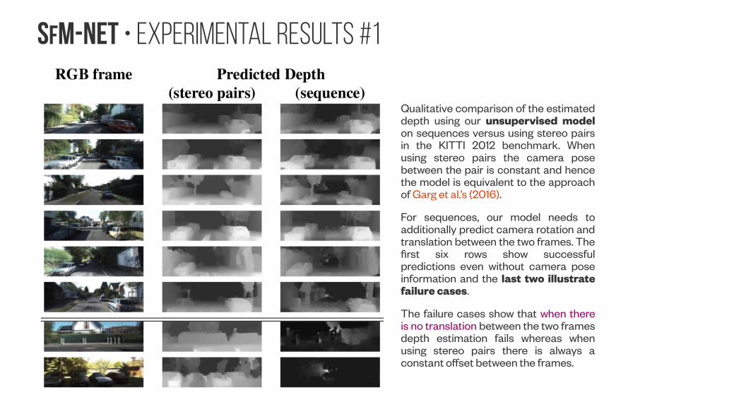
Qualitative comparison of the estimated depth using our unsupervised model on sequences versus using stereo pairs in the KITTI 2012 benchmark. When using stereo pairs the camera pose between the pair is constant and hence the model is equivalent to the approach of Garg et al.’s (2016).

For sequences, our model needs to additionally predict camera rotation and translation between the two frames. The first six rows show successful predictions even without camera pose information and the last two illustrate failure cases.

The failure cases show that when there is no translation between the two frames depth estimation fails whereas when using stereo pairs there is always a constant offset between the frames.

SfM-NeT • Experimental Results #2

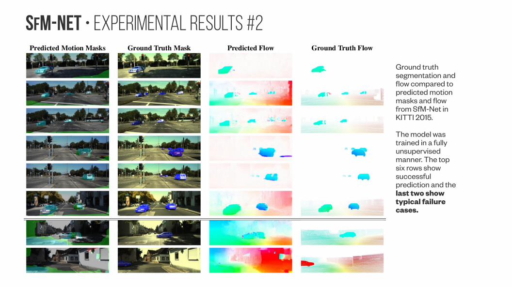
Ground truth segmentation and flow compared to predicted motion masks and flow from SfM-Net in KITTI 2015.

The model was trained in a fully unsupervised manner. The top six rows show successful prediction and the last two show typical failure cases.

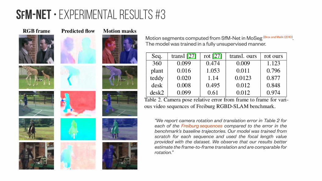
SfM-NeT • Experimental Results #3

Motion segments computed from SfM-Net in MoSeg [Brox and Malik (2010]. The model was trained in a fully unsupervised manner.

“We report camera rotation and translation error in Table 2 for each of the Freiburg sequences compared to the error in the benchmark’s baseline trajectories. Our model was trained from scratch for each sequence and used the focal length value provided with the dataset. We observe that our results better estimate the frame-to-frame translation and are comparable for rotation.”

SfM-Net • Summary

SfM-NeT • ConclusionCurrent geometric SLAM methods obtain excellent egomotion and rigid 3D reconstruction results, but often come at a price of extensive engineering, low tolerance to moving objects — which are treated as noise during reconstruction — and sensitivity to camera calibration.

Furthermore, matching and reconstruction are difficult in low textured regions. Incorporating learning into depth reconstruction, camera motion prediction and object segmentation, while still preserving the constraints of image formation,is a promising way to robustify SLAM and visual odometry even further. However, the exact training scenario required to solve this more difficult inference problem remains an open question.

Exploiting long history and far in time forward-backward constraints with visibility reasoning is an important future direction. Further, exploiting a small amount of annotated videos for object segmentation, depth, and camera motion, and combining those with an abundance of self-supervised videos, could help initialize the network weights in the right regime and facilitate learning. Many other curriculum learning regimes, including those that incorporate synthetic datasets, can also be considered

t geom

Future • Architecture

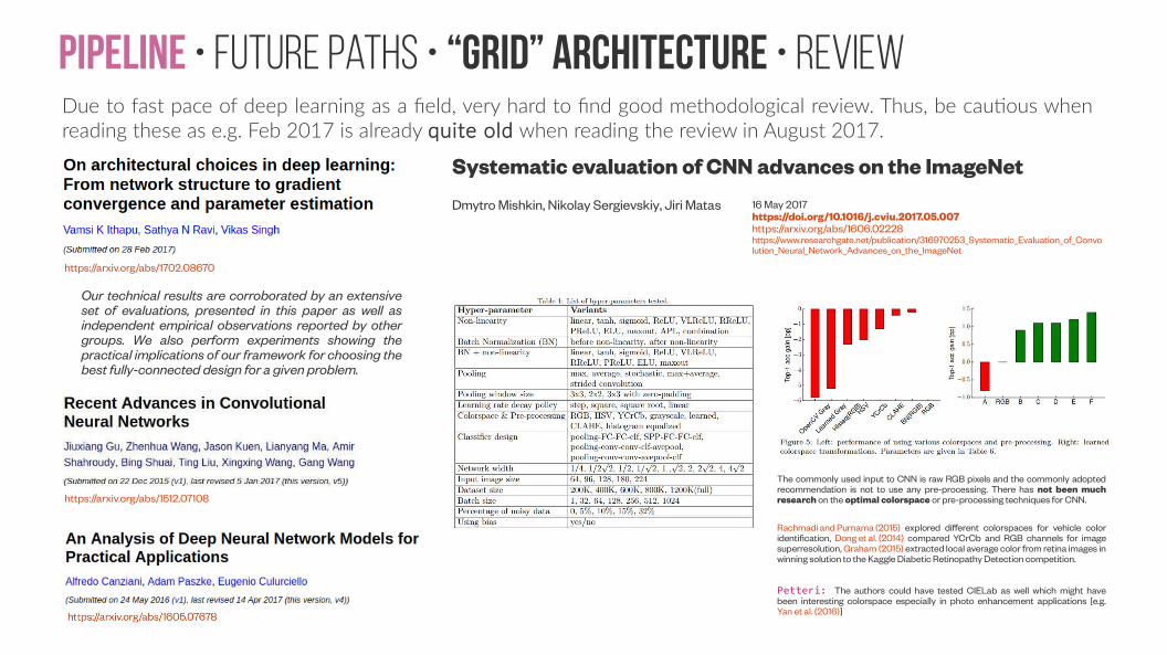
Pipeline • Future paths • “GRID” Architecture • Review

https://arxiv.org/abs/1702.08670

Our technical results are corroborated by an extensive set of evaluations, presented in this paper as well as independent empirical observations reported by other groups. We also perform experiments showing the practical implications of our framework for choosing the best fully-connected design for a given problem.

Due to fast pace of deep learning as a field, very hard to find good methodological review. Thus, be cautious when reading these as e.g. Feb 2017 is already quite old when reading the review in August 2017.

https://arxiv.org/abs/1512.07108

Systematic evaluation of CNN advances on the ImageNet

Dmytro Mishkin, Nikolay Sergievskiy, Jiri Matas 16 May 2017 https://doi.org/10.1016/j.cviu.2017.05.007https://arxiv.org/abs/1606.02228https://www.researchgate.net/publication/316970253_Systematic_Evaluation_of_Convolution_Neural_Network_Advances_on_the_ImageNet

The commonly used input to CNN is raw RGB pixels and the commonly adopted recommendation is not to use any pre-processing. There has not been much research on the optimal colorspace or pre-processing techniques for CNN.

Rachmadi and Purnama (2015) explored different colorspaces for vehicle color identification, Dong et al. (2014) compared YCrCb and RGB channels for image superresolution, Graham (2015) extracted local average color from retina images in winning solution to the Kaggle Diabetic Retinopathy Detection competition.

Petteri: The authors could have tested CIELab as well which might have been interesting colorspace especially in photo enhancement applications [e.g. Yan et al. (2016)]

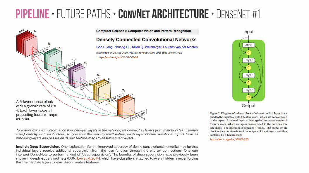
Pipeline • Future paths • ConvNet Architecture • DenseNet #1

To ensure maximum information flow between layers in the network, we connect all layers (with matching feature-map sizes) directly with each other. To preserve the feed-forward nature, each layer obtains additional inputs from all preceding layers and passes on its own feature-maps to all subsequent layers.

Implicit Deep Supervision. One explanation for the improved accuracy of dense convolutional networks may be that individual layers receive additional supervision from the loss function through the shorter connections. One can interpret DenseNets to perform a kind of “deep supervision”. The benefits of deep supervision have previously been shown in deeply-supervised nets (DSN; Lee et al. 2014), which have classifiers attached to every hidden layer, enforcing the intermediate layers to learn discriminative features.

https://arxiv.org/abs/1611.09326

Pipeline • Future paths • ConvNet Architecture • DenseNet #2

https://arxiv.org/abs/1608.06993

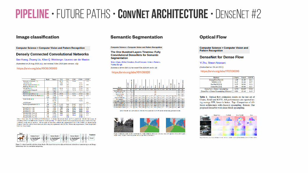
Image classification Semantic Segmentation Optical Flow

https://arxiv.org/abs/1611.09326 https://arxiv.org/abs/1707.06316

Pipeline • Future paths • ConvNet Architecture • DenseNet #3

https://arxiv.org/abs/1702.02295 https://arxiv.org/abs/1707.06316

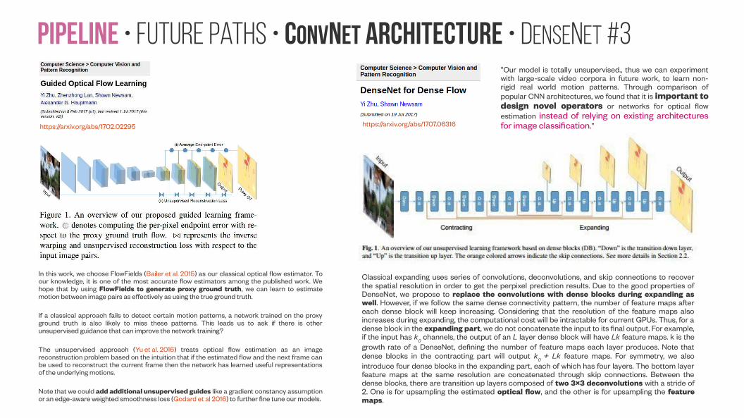
Classical expanding uses series of convolutions, deconvolutions, and skip connections to recover the spatial resolution in order to get the perpixel prediction results. Due to the good properties of DenseNet, we propose to replace the convolutions with dense blocks during expanding as well. However, if we follow the same dense connectivity pattern, the number of feature maps after each dense block will keep increasing. Considering that the resolution of the feature maps also increases during expanding, the computational cost will be intractable for current GPUs. Thus, for a dense block in the expanding part, we do not concatenate the input to its final output. For example, if the input has k

0 channels, the output of an L layer dense block will have Lk feature maps. k is the

growth rate of a DenseNet, defining the number of feature maps each layer produces. Note that dense blocks in the contracting part will output k

0 + Lk feature maps. For symmetry, we also

introduce four dense blocks in the expanding part, each of which has four layers. The bottom layer feature maps at the same resolution are concatenated through skip connections. Between the dense blocks, there are transition up layers composed of two 3×3 deconvolutions with a stride of 2. One is for upsampling the estimated optical flow, and the other is for upsampling the feature maps.

“Our model is totally unsupervised., thus we can experiment with large-scale video corpora in future work, to learn non-rigid real world motion patterns. Through comparison of popular CNN architectures, we found that it is important to design novel operators or networks for optical flow estimation instead of relying on existing architectures for image classification.”

In this work, we choose FlowFields (Bailer et al. 2015) as our classical optical flow estimator. To our knowledge, it is one of the most accurate flow estimators among the published work. We hope that by using FlowFields to generate proxy ground truth, we can learn to estimate motion between image pairs as effectively as using the true ground truth.

If a classical approach fails to detect certain motion patterns, a network trained on the proxy ground truth is also likely to miss these patterns. This leads us to ask if there is other unsupervised guidance that can improve the network training?

The unsupervised approach (Yu et al. 2016) treats optical flow estimation as an image reconstruction problem based on the intuition that if the estimated flow and the next frame can be used to reconstruct the current frame then the network has learned useful representations of the underlying motions.

Note that we could add additional unsupervised guides like a gradient constancy assumption or an edge-aware weighted smoothness loss (Godard et al 2016) to further fine tune our models.

Pipeline • Future paths • ConvNet Architecture • DenseNet #4

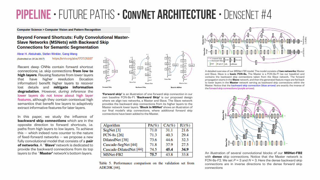
degradation. However, during inference the lower layers do not know about high layer features, although they contain contextual high semantics that benefit low layers to adaptively extract informative features for later layers.

In this paper, we study the influence of backward skip connections which are in the opposite direction to forward shortcuts, i.e. paths from high layers to low layers. To achieve this -- which indeed runs counter to the nature of feed-forward networks -- we propose a new fully convolutional model that consists of a pair of networks. A `Slave' network is dedicated to provide the backward connections from its top layers to the `Master' network's bottom layers.

‘Forward skip’ is an illustration of one forward skip connection in our own baseline FCN-8s-F1. ‘Backward Skip’ is our proposed design where we align two networks, a Master and Slave. The Slave network provides the backward skip connections from its higher layers to the Master network lower layers. ‘Block in MSNet’ shows an illustration of our final model’s skip connections, where additional forward skip connections have been added to the Master.

A detailed overview of our MSNet-FB1 model. The model consists of two networks; Master and Slave. Slave is a basic FCN-8s. The Master is a FCN-8s-F1 (as our baseline) and contains the backward skip connections taken from the Slave network. The forward propagation starts in the Slave network, and then the generated feature maps are fed back to lower layers in the Master network serving as backward skip connections within the Master. Notice that the backward skip connection (blue arrows) are exactly the inverse of the forward skip connections (purple arrows).

An illustration of several convolutional blocks of our MSNet-FB2 with dense skip connections. Notice that the Master network is FCN-8s-F2. We set P = 3 and N = 3. Here the dense backward skip connections are in inverse directions to the dense forward skip connections

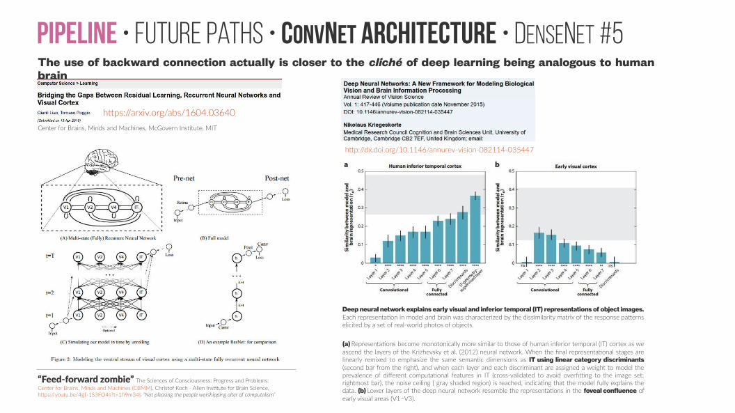
Pipeline • Future paths • ConvNet Architecture • DenseNet #5The use of backward connection actually is closer to the cliché of deep learning being analogous to human brain

Deep neural network explains early visual and inferior temporal (IT) representations of object images. Each representation in model and brain was characterized by the dissimilarity matrix of the response patterns elicited by a set of real-world photos of objects.

(a) Representations become monotonically more similar to those of human inferior temporal (IT) cortex as we ascend the layers of the Krizhevsky et al. (2012) neural network. When the final representational stages are linearly remixed to emphasize the same semantic dimensions as IT using linear category discriminants (second bar from the right), and when each layer and each discriminant are assigned a weight to model the prevalence of different computational features in IT (cross-validated to avoid overfitting to the image set; rightmost bar), the noise ceiling ( gray shaded region) is reached, indicating that the model fully explains the data. (b) Lower layers of the deep neural network resemble the representations in the foveal confluence of early visual areas (V1–V3).

http://dx.doi.org/10.1146/annurev-vision-082114-035447

https://arxiv.org/abs/1604.03640

Center for Brains, Minds and Machines, McGovern Institute, MIT

“Feed-forward zombie” The Sciences of Consciousness: Progress and Problems: Center for Brains, Minds and Machines (CBMM), Christof Koch - Allen Institute for Brain Science, https://youtu.be/4gT-1S3FO4s?t=1h9m34s “Not pleasing the people worshipping alter of computalism”

Pipeline • Future paths • Uncertainty • with DenseNet

https://arxiv.org/abs/1506.02142 https://arxiv.org/abs/1705.07832

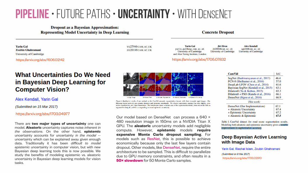
https://arxiv.org/abs/1703.04977

There are two major types of uncertainty one can model. Aleatoric uncertainty captures noise inherent in the observations. On the other hand, epistemic uncertainty accounts for uncertainty in the model -- uncertainty which can be explained away given enough data. Traditionally it has been difficult to model epistemic uncertainty in computer vision, but with new Bayesian deep learning tools this is now possible. We study the benefits of modeling epistemic vs. aleatoric uncertainty in Bayesian deep learning models for vision tasks.

Our model based on DenseNet can process a 640 × 480 resolution image in 150ms on a NVIDIA Titan X GPU. The aleatoric uncertainty models add negligible compute. However, epistemic models require expensive Monte Carlo dropout sampling. For models such as ResNet, this is possible to achieve economically because only the last few layers contain dropout. Other models, like DenseNet, require the entire architecture to be sampled. This is difficult to parallelize due to GPU memory constraints, and often results in a 50× slowdown for 50 Monte Carlo samples.

https://arxiv.org/abs/1703.02910

Pipeline • Future paths • Uncertainty • With model compressionBayesian Compression for Deep LearningChristos Louizos, Karen Ullrich, Max Welling(Submitted on 24 May 2017 (v1), last revised 10 Aug 2017 (this version, v3))https://arxiv.org/abs/1705.08665

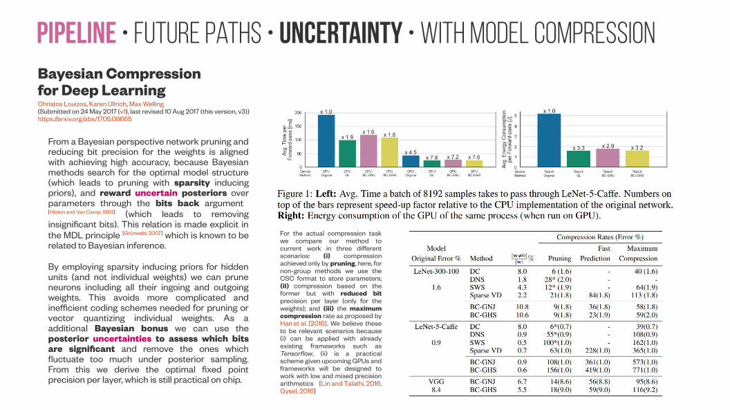
From a Bayesian perspective network pruning and reducing bit precision for the weights is aligned with achieving high accuracy, because Bayesian methods search for the optimal model structure (which leads to pruning with sparsity inducing priors), and reward uncertain posteriors over parameters through the bits back argument [Hinton and Van Camp, 1993] (which leads to removing insignificant bits). This relation is made explicit in the MDL principle [Grünwald, 2007] which is known to be related to Bayesian inference.

By employing sparsity inducing priors for hidden units (and not individual weights) we can prune neurons including all their ingoing and outgoing weights. This avoids more complicated and inefficient coding schemes needed for pruning or vector quantizing individual weights. As a additional Bayesian bonus we can use the posterior uncertainties to assess which bits are significant and remove the ones which fluctuate too much under posterior sampling. From this we derive the optimal fixed point precision per layer, which is still practical on chip.

For the actual compression task we compare our method to current work in three different scenarios: (i) compression achieved only by pruning, here, for non-group methods we use the CSC format to store parameters; (ii) compression based on the former but with reduced bit precision per layer (only for the weights); and (iii) the maximum compression rate as proposed by Han et al. [2016]. We believe these to be relevant scenarios because (i) can be applied with already existing frameworks such as Tensorflow, (ii) is a practical scheme given upcoming GPUs and frameworks will be designed to work with low and mixed precision arithmetics [Lin and Talathi, 2016, Gysel, 2016]

Pipeline • Future paths • Uncertainty • Geometric problems

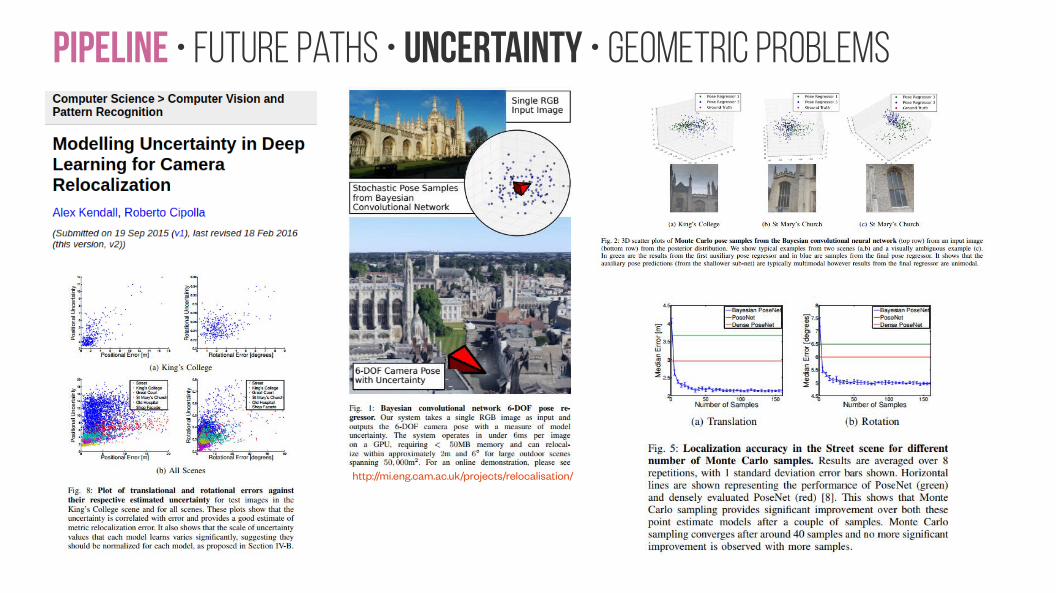
http://mi.eng.cam.ac.uk/projects/relocalisation/

Future • Geometric Architectures

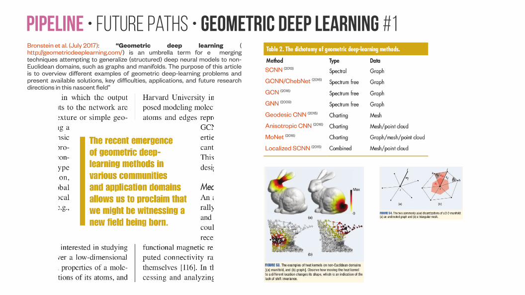
Pipeline • Future paths • Geometric Deep Learning #1Bronstein et al. (July 2017): “Geometric deep learning (http://geometricdeeplearning.com/) is an umbrella term for e merging techniques attempting to generalize (structured) deep neural models to non-Euclidean domains, such as graphs and manifolds. The purpose of this article is to overview different examples of geometric deep-learning problems and present available solutions, key difficulties, applications, and future research directions in this nascent field”

SCNN (2013)

GCNN/ChebNet (2016)

GCN (2016)

GNN (2009)

Geodesic CNN (2015)

Anisotropic CNN (2016)

MoNet (2016)

Localized SCNN (2015)

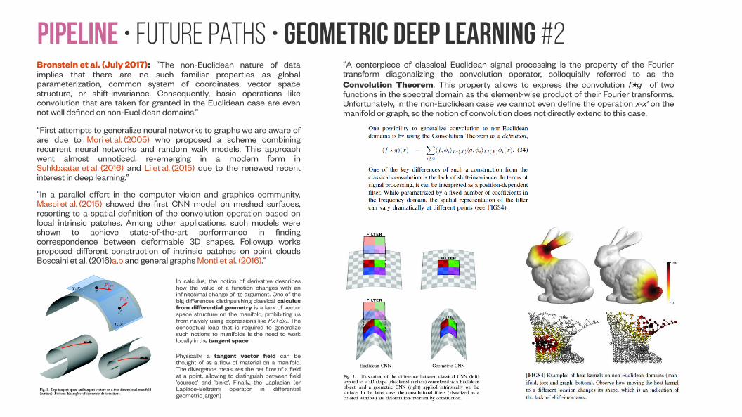
Pipeline • Future paths • Geometric Deep Learning #2Bronstein et al. (July 2017): “The non-Euclidean nature of data implies that there are no such familiar properties as global parameterization, common system of coordinates, vector space structure, or shift-invariance. Consequently, basic operations like convolution that are taken for granted in the Euclidean case are even not well defined on non-Euclidean domains.”

“First attempts to generalize neural networks to graphs we are aware of are due to Mori et al. (2005) who proposed a scheme combining recurrent neural networks and random walk models. This approach went almost unnoticed, re-emerging in a modern form in Suhkbaatar et al. (2016) and Li et al. (2015) due to the renewed recent interest in deep learning.”

“In a parallel effort in the computer vision and graphics community, Masci et al. (2015) showed the first CNN model on meshed surfaces, resorting to a spatial definition of the convolution operation based on local intrinsic patches. Among other applications, such models were shown to achieve state-of-the-art performance in finding correspondence between deformable 3D shapes. Followup works proposed different construction of intrinsic patches on point clouds Boscaini et al. (2016)a,b and general graphs Monti et al. (2016).”

In calculus, the notion of derivative describes how the value of a function changes with an infinitesimal change of its argument. One of the big differences distinguishing classical calculus from differential geometry is a lack of vector space structure on the manifold, prohibiting us from naïvely using expressions like f(x+dx). The conceptual leap that is required to generalize such notions to manifolds is the need to work locally in the tangent space.

Physically, a tangent vector field can be thought of as a flow of material on a manifold. The divergence measures the net flow of a field at a point, allowing to distinguish between field ‘sources’ and ‘sinks’. Finally, the Laplacian (or Laplace-Beltrami operator in differential geometric jargon)

“A centerpiece of classical Euclidean signal processing is the property of the Fourier transform diagonalizing the convolution operator, colloquially referred to as the Convolution Theorem. This property allows to express the convolution f⋆g of two functions in the spectral domain as the element-wise product of their Fourier transforms. Unfortunately, in the non-Euclidean case we cannot even define the operation x-x’ on the manifold or graph, so the notion of convolution does not directly extend to this case.

Pipeline • Future paths • Geometric Deep Learning #3Bronstein et al. (July 2017): “We expect the following years to bring exciting new approaches and results, and conclude our review with a few observations of current key difficulties and potential directions of future research.”

Generalization: Generalizing deep learning models to geometric data requires not only finding non-Euclidean counterparts of basic building blocks (such as convolutional and pooling layers), but also generalization across different domains. Generalization capability is a key requirement in many applications, including computer graphics, where a model is learned on a training set of non-Euclidean domains (3D shapes) and then applied to previously unseen ones.

Time-varying domains: An interesting extension of geometric deep learning problems discussed in this review is coping with signals defined over a dynamically changing structure. In this case, we cannot assume a fixed domain and must track how these changes affect signals. This could prove useful to tackle applications such as abnormal activity detection in social or financial networks. In the domain of computer graphics and vision, potential applications deal with dynamic shapes (e.g. 3D video captured by a range sensor).

Computation: The final consideration is a computational one. All existing deep learning software frameworks are primarily optimized for Euclidean data. One of the main reasons for the computational efficiency of deep learning architectures (and one of the factors that contributed to their renaissance) is the assumption of regularly structured data on 1D or 2D grid, allowing to take advantage of modern GPU hardware. Geometric data, on the other hand, in most cases do not have a grid structure, requiring different ways to achieve efficient computations. It seems that computational paradigms developed for large-scale graph processing are more adequate frameworks for such applications.

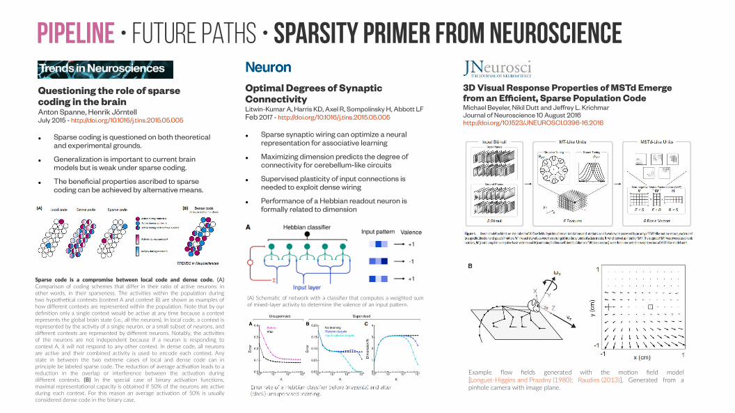
Pipeline • Future paths • sparsity primer from neuroscience

Questioning the role of sparse coding in the brainAnton Spanne, Henrik JörntellJuly 2015 - http://doi.org/10.1016/j.tins.2015.05.005

Optimal Degrees of Synaptic ConnectivityLitwin-Kumar A, Harris KD, Axel R, Sompolinsky H, Abbott LFFeb 2017 - http://doi.org/10.1016/j.tins.2015.05.005

3D Visual Response Properties of MSTd Emerge from an Efficient, Sparse Population CodeMichael Beyeler, Nikil Dutt and Jeffrey L. KrichmarJournal of Neuroscience 10 August 2016http://doi.org/10.1523/JNEUROSCI.0396-16.2016

● Sparse coding is questioned on both theoretical and experimental grounds.

● Generalization is important to current brain models but is weak under sparse coding.

● The beneficial properties ascribed to sparse coding can be achieved by alternative means.

Sparse code is a compromise between local code and dense code. (A) Comparison of coding schemes that differ in their ratio of active neurons: in other words, in their sparseness. The activities within the population during two hypothetical contexts (context A and context B) are shown as examples of how different contexts are represented within the population. Note that by our definition only a single context would be active at any time because a context represents the global brain state (i.e., all the neurons). In local code, a context is represented by the activity of a single neuron, or a small subset of neurons, and different contexts are represented by different neurons. Notably, the activities of the neurons are not independent because if a neuron is responding to context A, it will not respond to any other context. In dense code, all neurons are active and their combined activity is used to encode each context. Any state in between the two extreme cases of local and dense code can in principle be labeled sparse code. The reduction of average activation leads to a reduction in the overlap or interference between the activation during different contexts. (B) In the special case of binary activation functions, maximal representational capacity is obtained if 50% of the neurons are active during each context. For this reason an average activation of 50% is usually considered dense code in the binary case.

● Sparse synaptic wiring can optimize a neural representation for associative learning

● Maximizing dimension predicts the degree of connectivity for cerebellum-like circuits

● Supervised plasticity of input connections is needed to exploit dense wiring

● Performance of a Hebbian readout neuron is formally related to dimension

(A) Schematic of network with a classifier that computes a weighted sum of mixed-layer activity to determine the valence of an input pattern.

Example flow fields generated with the motion field model[Longuet-Higgins and Prazdny (1980); Raudies (2013)]. Generated from a pinhole camera with image plane.

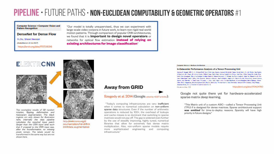
Pipeline • Future paths • Non-euclidean computability & Geometric Operators #1

https://arxiv.org/abs/1707.06316

“Our model is totally unsupervised., thus we can experiment with large-scale video corpora in future work, to learn non-rigid real world motion patterns. Through comparison of popular CNN architectures, we found that it is important to design novel operators or networks for optical flow estimation instead of relying on existing architectures for image classification”

pixels remain. The labels would be transformed in the same way but are not shown here.

Away from GRID

Szegedy et al. 2014 (Google, cited by 4,027 articles):

“Today’s computing infrastructures are very inefficient when it comes to numerical calculation on non-uniform sparse data structures. Even if the number of arithmetic operations is reduced by 100×, the overhead of lookups and cache misses is so dominant that switching to sparse matrices would not pay off. The gap is widened even further by the use of steadily improving, highly tuned, numerical libraries that allow for extremely fast dense matrix multiplication. Also, non-uniform sparse models require more sophisticated engineering and computing infrastructure.”

https://arxiv.org/abs/1704.04760

Google not quite there yet for hardware-accelerated sparse matrix deep learning.

“This Matrix unit of a custom ASIC—called a Tensor Processing Unit (TPU) if is designed for dense matrices. Sparse architectural support was omitted for time-to-deploy reasons. Sparsity will have high priority in future designs.”

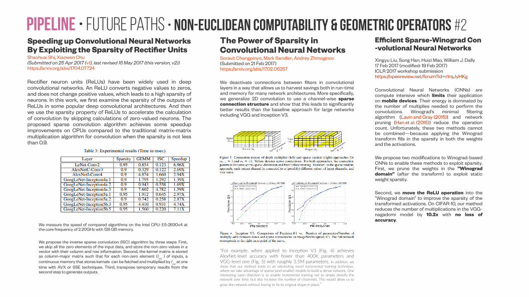
Pipeline • Future paths • Non-euclidean computability & Geometric Operators #2Speeding up Convolutional Neural Networks By Exploiting the Sparsity of Rectifier UnitsShaohuai Shi, Xiaowen Chu(Submitted on 25 Apr 2017 (v1), last revised 15 May 2017 (this version, v2))https://arxiv.org/abs/1704.07724

Rectifier neuron units (ReLUs) have been widely used in deep convolutional networks. An ReLU converts negative values to zeros, and does not change positive values, which leads to a high sparsity of neurons. In this work, we first examine the sparsity of the outputs of ReLUs in some popular deep convolutional architectures. And then we use the sparsity property of ReLUs to accelerate the calculation of convolution by skipping calculations of zero-valued neurons. The proposed sparse convolution algorithm achieves some speedup improvements on CPUs compared to the traditional matrix-matrix multiplication algorithm for convolution when the sparsity is not less than 0.9.

We measure the speed of compared algorithms on the Intel CPU: E5-2630v4 at the core frequency of 2.20GHz with 128 GB memory.

We propose the inverse sparse convolution (ISC) algorithm by three steps: First, we skip all the zero elements of the input data, and store the non-zero values in a vector with their column and row information. Second, the kernel matrix is stored as column-major matrix such that for each non-zero element (Ic,i,j ) of inputs, a continuous memory that stores kernels can be fetched and multiplied by I

c,i,j at one

time with AVX or SSE techniques. Third, transpose temporary results from the second step to generate outputs.

The Power of Sparsity in Convolutional Neural NetworksSoravit Changpinyo, Mark Sandler, Andrey Zhmoginov (Submitted on 21 Feb 2017)https://arxiv.org/abs/1702.06257

We deactivate connections between filters in convolutional layers in a way that allows us to harvest savings both in run-time and memory for many network architectures. More specifically, we generalize 2D convolution to use a channel-wise sparse connection structure and show that this leads to significantly better results than the baseline approach for large networks including VGG and Inception V3.

“For example, when applied to Inception V3 (Fig. 4) achieves AlexNet-level accuracy with fewer than 400K parameters and VGG-level one (Fig. 5) with roughly 3.5M parameters. In addition, we show that our method leads to an interesting novel incremental training technique, where we take advantage of sparse (and smaller) models to build a dense network. One interesting open direction is to enable incremental training not to simply densify the network over time, but also increase the number of chaannels. This would allow us to grow the network without having to fix its original shape in place.”

Efficient Sparse-Winograd Con-volutional Neural NetworksXingyu Liu, Song Han, Huizi Mao, William J. Dally17 Feb 2017 (modified: 19 Feb 2017)ICLR 2017 workshop submissionhttps://openreview.net/forum?id=r1rqJyHKg

Convolutional Neural Networks (CNNs) are compute intensive which limits their application on mobile devices. Their energy is dominated by the number of multiplies needed to perform the convolutions. Winograd’s minimal filtering algorithm (Lavin and Gray (2015)) and network pruning (Han et al. (2015)) reduce the operation count. Unfortunately, these two methods cannot be combined—because applying the Winograd transform fills in the sparsity in both the weights and the activations.

We propose two modifications to Winograd-based CNNs to enable these methods to exploit sparsity. First, we prune the weights in the ”Winograd domain” (after the transform) to exploit static weight sparsity.

Second, we move the ReLU operation into the ”Winograd domain” to improve the sparsity of the transformed activations. On CIFAR-10, our method reduces the number of multiplications in the VGG-nagadomi model by 10.2x with no loss of accuracy.

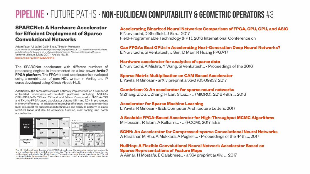
Pipeline • Future paths • Non-euclidean computability & Geometric Operators #3SPARCNet: A Hardware Accelerator for Efficient Deployment of Sparse Convolutional NetworksAdam Page, Ali Jafari, Colin Shea, Tinoosh MohseninACM Journal on Emerging Technologies in Computing Systems (JETC) - Special Issue on Hardware and Algorithms for Learning On-a-chip and Special Issue on Alternative Computing Systems.Volume 13 Issue 3, May 2017 - Article No. 31. https://doi.org/10.1145/3005448

The SPARCNet accelerator with different numbers of processing engines is implemented on a low-power Artix-7 FPGA platform. The FPGA-based accelerator is developed using a combination of pure HDL written in Verilog and IP cores developed using Xilinx’s Vivado HLS.

Additionally, the same networks are optimally implemented on a number of embedded commercial-off-the-shelf platforms including NVIDIAs CPU+GPU SoCs TK1 and TX1 and Intel Edison. Compared to NVIDIAs TK1 and TX1, the FPGA-based accelerator obtains 11.8 × and 7.5 × improvement in energy efficiency In addition to improving efficiency, the accelerator has built-in support for sparsification techniques and ability to perform in-place rectified linear unit (ReLU) activation function, max-pooling, and batch normalization.

Accelerating Binarized Neural Networks: Comparison of FPGA, CPU, GPU, and ASICE Nurvitadhi, D Sheffield, J Sim… 2017 Field-Programmable Technology (FPT), 2016 International Conference on

Can FPGAs Beat GPUs in Accelerating Next-Generation Deep Neural Networks?E Nurvitadhi, G Venkatesh, J Sim, D Marr, R Huang FPGA’17

Hardware accelerator for analytics of sparse dataE Nurvitadhi, A Mishra, Y Wang, G Venkatesh… - Proceedings of the 2016

Sparse Matrix Multiplication on CAM Based AcceleratorL Yavits, R Ginosar - arXiv preprint arXiv:1705.09937, 2017

Cambricon-X: An accelerator for sparse neural networksS Zhang, Z Du, L Zhang, H Lan, S Liu… - … (MICRO), 2016 49th …, 2016

Accelerator for Sparse Machine LearningL Yavits, R Ginosar - IEEE Computer Architecture Letters, 2017

A Scalable FPGA-Based Accelerator for High-Throughput MCMC AlgorithmsM Hosseini, R Islam, A Kulkarni… - … (FCCM), 2017 IEEE

SCNN: An Accelerator for Compressed-sparse Convolutional Neural NetworksA Parashar, M Rhu, A Mukkara, A Puglielli… - Proceedings of the 44th …, 2017

NullHop: A Flexible Convolutional Neural Network Accelerator Based on Sparse Representations of Feature MapsA Aimar, H Mostafa, E Calabrese… - arXiv preprint arXiv: …, 2017

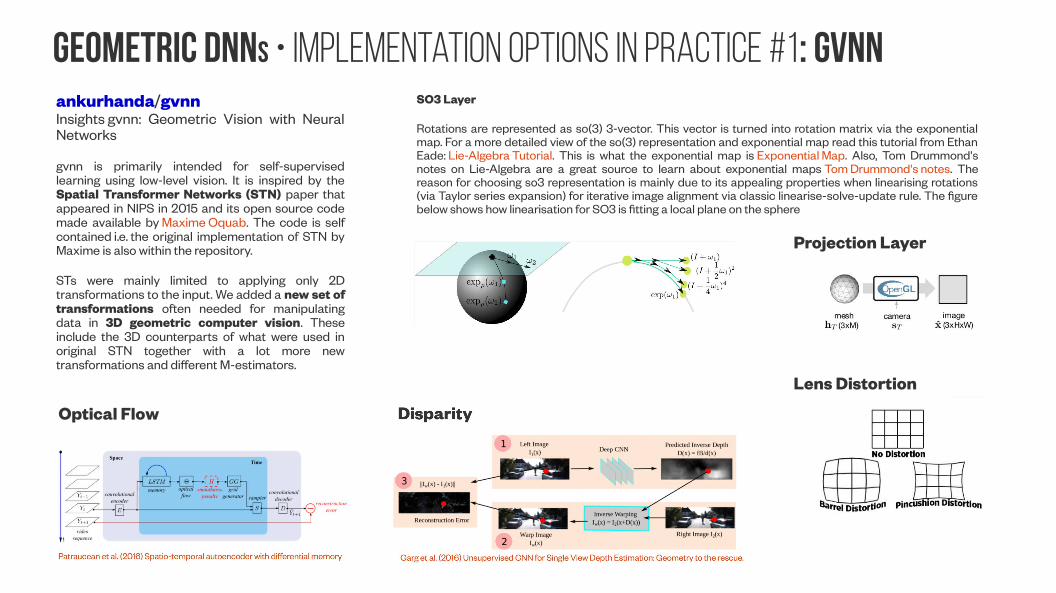
Geometric DNNs • implementation options in practice #1: GVNNankurhanda/gvnnInsights gvnn: Geometric Vision with Neural Networks

gvnn is primarily intended for self-supervised learning using low-level vision. It is inspired by the Spatial Transformer Networks (STN) paper that appeared in NIPS in 2015 and its open source code made available by Maxime Oquab. The code is self contained i.e. the original implementation of STN by Maxime is also within the repository.

STs were mainly limited to applying only 2D transformations to the input. We added a new set of transformations often needed for manipulating data in 3D geometric computer vision. These include the 3D counterparts of what were used in original STN together with a lot more new transformations and different M-estimators.

SO3 Layer

Rotations are represented as so(3) 3-vector. This vector is turned into rotation matrix via the exponential map. For a more detailed view of the so(3) representation and exponential map read this tutorial from Ethan Eade: Lie-Algebra Tutorial. This is what the exponential map is Exponential Map. Also, Tom Drummond's notes on Lie-Algebra are a great source to learn about exponential maps Tom Drummond's notes. The reason for choosing so3 representation is mainly due to its appealing properties when linearising rotations (via Taylor series expansion) for iterative image alignment via classic linearise-solve-update rule. The figure below shows how linearisation for SO3 is fitting a local plane on the sphere

Optical Flow

Lens Distortion

Projection Layer