1

The Computational Problem of Structure from Motion (SFM)

Structure from Motion (SFM)

• People spend a large portion of their time in locomotion. Every time we change the position of our eyes or head, retinal motion is produced. – dominant stimulus for normal everyday vision.

• Role for biological vision– Find direction of heading (navigation and stabilization)– Cues to depth and shape (compare with stereo)– Avoid obstacles when moving– Find other objects approaching/leaving (hunt/escape)– Figure-ground segmentation / object segmentation (similar

velocities and /or depths)– Controlling eye movements (saccades and smooth pursuit)

2

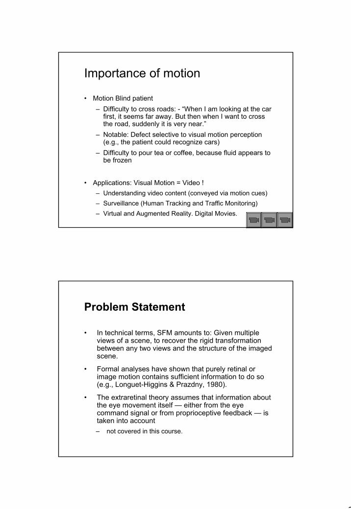
Importance of motion

• Motion Blind patient– Difficulty to cross roads: - “When I am looking at the car

first, it seems far away. But then when I want to cross the road, suddenly it is very near.”

– Notable: Defect selective to visual motion perception (e.g., the patient could recognize cars)

– Difficulty to pour tea or coffee, because fluid appears to be frozen

• Applications: Visual Motion = Video ! – Understanding video content (conveyed via motion cues)– Surveillance (Human Tracking and Traffic Monitoring)– Virtual and Augmented Reality. Digital Movies.

Problem Statement

• In technical terms, SFM amounts to: Given multiple views of a scene, to recover the rigid transformationbetween any two views and the structure of the imaged scene.

• Formal analyses have shown that purely retinal or image motion contains sufficient information to do so (e.g., Longuet-Higgins & Prazdny, 1980).

• The extraretinal theory assumes that information about the eye movement itself — either from the eye command signal or from proprioceptive feedback — is taken into account – not covered in this course.

3

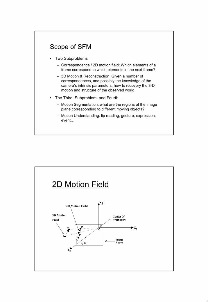
Scope of SFM• Two Subproblems

– Correspondence / 2D motion field: Which elements of a frame correspond to which elements in the next frame?

– 3D Motion & Reconstruction :Given a number of correspondences, and possibly the knowledge of the camera’s intrinsic parameters, how to recovery the 3-D motion and structure of the observed world

• The Third Subproblem, and Fourth….– Motion Segmentation: what are the regions of the image

plane corresponding to different moving objects?

– Motion Understanding: lip reading, gesture, expression, event…

2D Motion Field

2D Motion Field

3D Motion Field

4

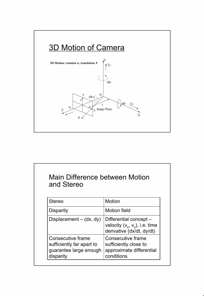
3D Motion of Camera yT

yω

zω

xω xT zT

Y

f

X

Y O

XZ Image Plane

O

P

3D Motion: rotation w, translation T

Main Difference between Motion and Stereo

Consecutive frame sufficiently close to approximate differential conditions

Consecutive frame sufficiently far apart to guarantee large enough disparity

Differential concept –velocity (vx, vy), i.e. time derivative (dx/dt, dy/dt)

Displacement – (dx, dy)

Motion fieldDisparity

MotionStereo

5

2D Motion Estimation

• Three prevalent approaches to computing 2D Motion Field: -- gradient techniques

» obtain 2D image flow / optical flow from spatial and temporal image intensity derivatives.

-- token/feature matching or correlation» similar to the methods covered in stereo

-- velocity sensitive filters» frequency domain models of motion estimation» not covered in this course.

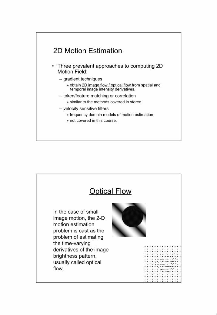
Optical Flow

In the case of small image motion, the 2-D motion estimation problem is cast as the problem of estimating the time-varying derivatives of the image brightness pattern, usually called optical flow.

6

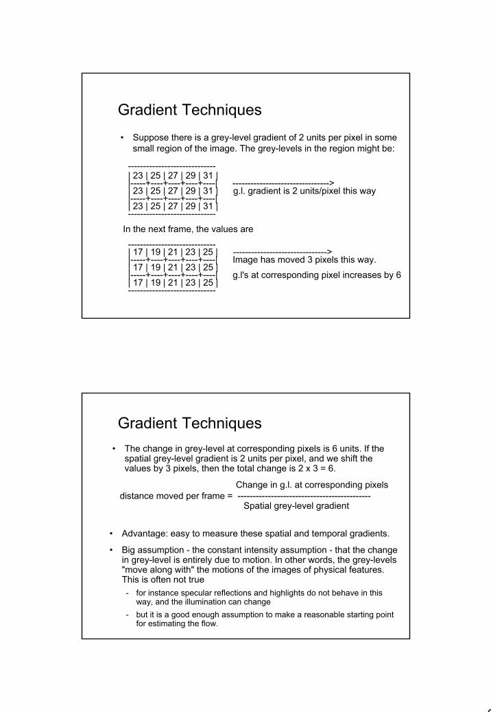
Gradient Techniques• Suppose there is a grey-level gradient of 2 units per pixel in some

small region of the image. The grey-levels in the region might be:

-----------------------------| 23 | 25 | 27 | 29 | 31 ||-----+----+----+----+----| -------------------------------->| 23 | 25 | 27 | 29 | 31 | g.l. gradient is 2 units/pixel this way|-----+----+----+----+----|| 23 | 25 | 27 | 29 | 31 |-----------------------------

In the next frame, the values are

-----------------------------| 17 | 19 | 21 | 23 | 25 | ------------------------------->|-----+----+----+----+----| Image has moved 3 pixels this way.| 17 | 19 | 21 | 23 | 25 ||-----+----+----+----+----| g.l's at corresponding pixel increases by 6| 17 | 19 | 21 | 23 | 25 |-----------------------------

Gradient Techniques• The change in grey-level at corresponding pixels is 6 units. If the

spatial grey-level gradient is 2 units per pixel, and we shift the values by 3 pixels, then the total change is 2 x 3 = 6.

Change in g.l. at corresponding pixelsdistance moved per frame = --------------------------------------------

Spatial grey-level gradient

• Advantage: easy to measure these spatial and temporal gradients.

• Big assumption - the constant intensity assumption - that the change in grey-level is entirely due to motion. In other words, the grey-levels "move along with" the motions of the images of physical features. This is often not true - for instance specular reflections and highlights do not behave in this

way, and the illumination can change- but it is a good enough assumption to make a reasonable starting point

for estimating the flow.

7

Gradient Techniques

• Assume E(x,y,t) is a continuous and differentiable function of space and time

• Suppose the brightness pattern is locally displaced by a distance dx, dy over time period dt. -- we assume that as the time varying image evolves, the image

brightness of points don't change as they move in the image

E(x,y,t) = E(x + dx, y + dy, t + dt)

0=dtdE

– In other word, the total derivative of E w.r.t. time is zero.

Gradient Techniques

tE

dtdy

yE

dtdx

xE

dtdE

δδ

δδ

δδ0 ++==

• Expanding E(x + dx, y + dy, t + dt) in a Taylor series & divide by dt:

• Can write as dE/dt = = ∇ET (vx,vy) + Et = 0.

-- The ∇E and Et are derivatives measured from the image

-- (vx,vy) are the unknown optic flow components (dx/dt,dy/dt) in the x and y directions, respectively

• This equation is known as the Brightness Constancy Equation (BCE) -- valid only if intensity change is due entirely to motion

0x x y y tE v E v E+ + =

8

Aperture Problem

• Beside the constant brightness assumption, there is a further problem.– In the example above, a motion along the y-axis will not

have any effect on the grey levels– We only have information about motion along the x-axis

in this case, or in general along the grey-level gradient. – This component of motion is sometimes called the edge

motion; it is at right-angles to the local edge direction.

• This effect is a manifestation of what is known as the aperture problem, because it is a result of considering a local region of the image only.

-----------------------------| 23 | 25 | 27 | 29 | 31 ||-----+----+----+----+----| | 23 | 25 | 27 | 29 | 31 | |-----+----+----+----+----|| 23 | 25 | 27 | 29 | 31 |-----------------------------

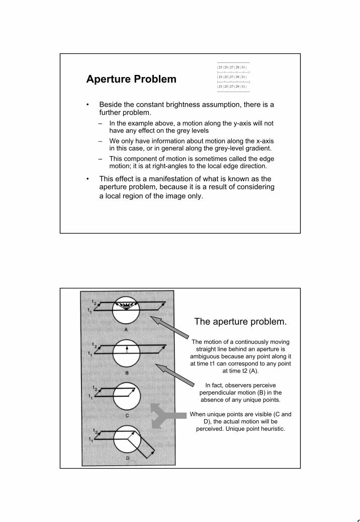
The aperture problem.

The motion of a continuously moving straight line behind an aperture is

ambiguous because any point along it at time t1 can correspond to any point

at time t2 (A).

In fact, observers perceive perpendicular motion (B) in the absence of any unique points.

When unique points are visible (C and D), the actual motion will be

perceived. Unique point heuristic.

9

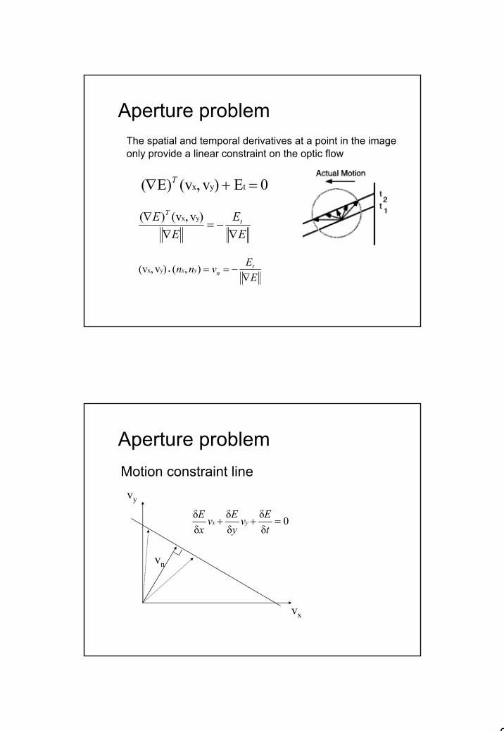
Aperture problem

EEvnn t

nyx∇

−==• ),()v,(v yx

EE

EE t

T

∇−=

∇∇ )v,(v)( yx

The spatial and temporal derivatives at a point in the image only provide a linear constraint on the optic flow

0 E )v,(vE)( tyx =+∇ T

Aperture problemMotion constraint linevy

vn

vx

0δδ

δδ

δδ

=++tEv

yEv

xE

yx

10

Constraining the BCE• Three common approaches:

- impose smoothness constraint on flow (H+S)• Solution: iterative scheme minimizing departure of (u,v) from

smoothness.

- assume velocity is locally constant (L+K) • Solution: Least square of two variables (u,v) from NxN Equations in

the NxN window

- assume local parametric model (eg affine, uT = ApT+b ). • Solution: Least square of 6 variables (A,b) from NxN

• All methods combine information from a larger region. Other approaches also exist.

Horn and Schunck’s algorithm

H+S assumptions: Flow field are varying smoothly within a small patch

+∇= tT

b EEE )v,(v)( yx

The error in the optical flow constraint equation should be small too

2y2y2x2x2 vvvv

∂∂

+

∂∂

+

∂∂

+

∂∂

=yxyx

Ec

Thus we shall try to minimize a measure of departure from smoothness

( ) dydxEE bc∫∫ + 222min α

Solve using calculus of variation Known as regularization approach.

big α : put emphasis on regularity small α: put emphasis on the optical flow constraint equation

11

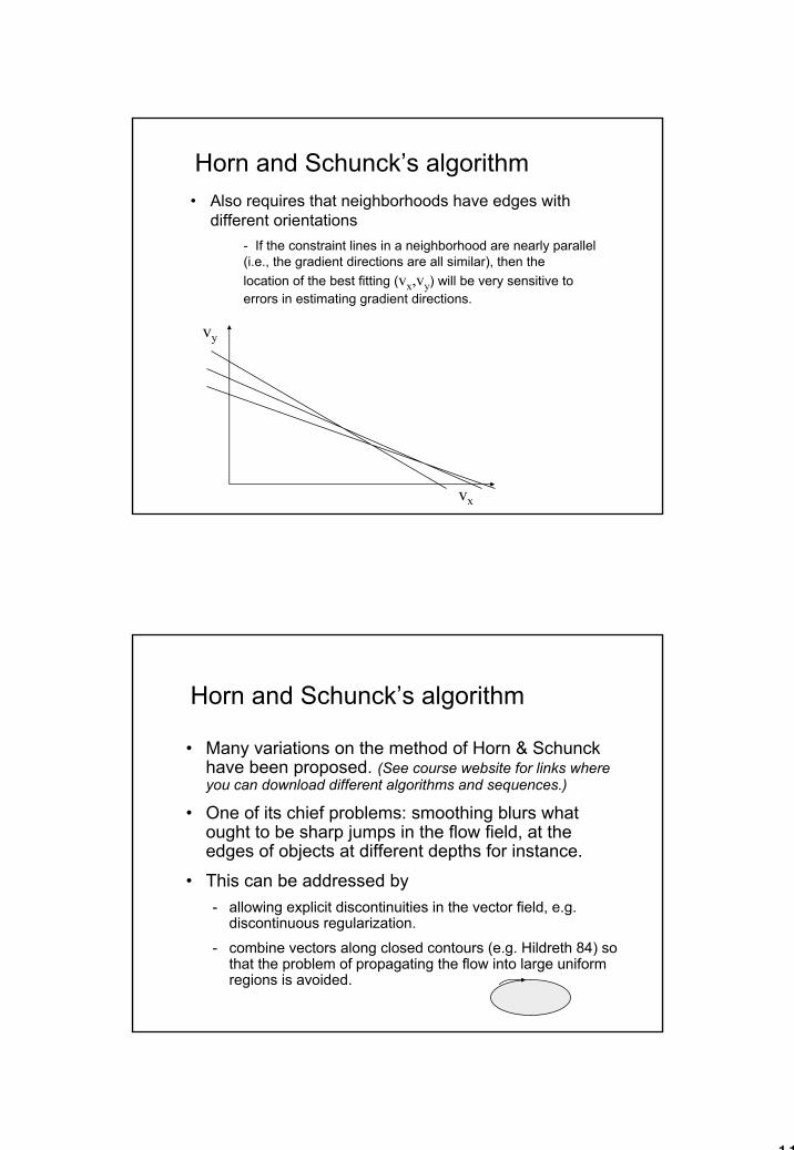
• Also requires that neighborhoods have edges with different orientations

vy

vx

Horn and Schunck’s algorithm

- If the constraint lines in a neighborhood are nearly parallel(i.e., the gradient directions are all similar), then the location of the best fitting (vx,vy) will be very sensitive to errors in estimating gradient directions.

Horn and Schunck’s algorithm

• Many variations on the method of Horn & Schunckhave been proposed. (See course website for links where you can download different algorithms and sequences.)

• One of its chief problems: smoothing blurs what ought to be sharp jumps in the flow field, at the edges of objects at different depths for instance.

• This can be addressed by - allowing explicit discontinuities in the vector field, e.g.

discontinuous regularization.

- combine vectors along closed contours (e.g. Hildreth 84) so that the problem of propagating the flow into large uniform regions is avoided.

12

Interlude: A regularization approach• Many vision problems such as stereo reconstruction of visible

surfaces and recovery of optic flow are instances of ill posedproblems.

• A problem is well posed when its solution (Hadamard’s definition): -- exists -- is unique, and -- depends continuously on its initial data

• Any problem that is not well posed is said to be ill posed

• The optic flow problem is to recover both degress of freedom of motion at each image pixel, given the spatial and temporal derivatives of the image sequence -- but any solution chosen at each pixel that locally satisfies the motion

constraint equation can be used to construct an optic flow fieldconsistent with the derivatives measured

-- therefore, the solution is not unique - how to choose one?

A regularization approach• Solution - add a priori knowledge that can choose between the

solutions

• Formally, suppose we have an ill posed problem of determining z from data y expressed as -- Az = y, where A is a linear operator (e.g., projection operation in

image formation)

• We must choose a quadratic norm || || and a so-called stabilizing functional || Pz || and then find the z that minimizes: -- ||Az-y|| 2 + ||Pz|| 2

-- controls the compromise between the degree of regularization and the closeness of the solution to the input data (the first term).

λλ

• T. Poggio, V. Torre and C. Koch, Computational vision and regularization theory, Nature, 317, 1984.

13

A regularization approach• A regularization approach for optic flow:

2yx

2 ||)v,(v)(|||||| +∇= tT

dtdE EE-- the first term is

2y2y2x2x2 vvvv

∂∂

+

∂∂

+

∂∂

+

∂∂

=yxyx

Ec

-- the second term enforces a smoothness constraint on the optic flow field :

-- The regularization problem is then to find a flow field that minimizes both terms.

-- This minimization can be done over the entire image using various iterative techniques (calculus of variation; not needed).

The Lucas & Kanade Algorithm

• Assume motion field at given time, v(x; y), is constant over a block of pixels B

• Not unreasonable for small blocks in homogeneous motion regions

• Error in BCE over block is then 2

yx ))v,(v)(( +∇= ∑ tT EEε

• Estimated motion at centre of block is then the flow which minimises . Typical least square problem.ε

• Repeat procedure for all point

14

L&K Algorithm: Example

• Error in BCE over 3x3 block B is

2x y

,

x

y

( ( ) ( v , v ) )

vv :: :

Tt

x y B

t

E E

E E Ex y

ε∈

= ∇ +

∂ ∂ − ∂ ∂ =

∑

-----------------------------| 23 | 25 | 27 | 29 | 31 |-----------------------------| 23 | 25 | 27 | 29 | 31 | -----------------------------| 23 | 25 | 27 | 29 | 31 |-----------------------------|23 | 25 | 27 | 29 | 31 |-----------------------------|23 | 25 | 27 | 29 | 31 |-----------------------------

at time t0

-----------------------------| 17 | 19 | 21 | 23 | 25 | -----------------------------| 17 | 19 | 21 | 23 | 25 |-----------------------------| 17 | 19 | 21 | 23 | 25 |-----------------------------| 17 | 19 | 21 | 23 | 25 |-----------------------------| 17 | 19 | 21 | 23 | 25 |-----------------------------

at time t1

3x3 Block B

x

y

2 0 6v

2 0 :v

: : :

=

Assume: derivative computed using forward difference. Spatial derivatives computed using frame at t0 only.

9 equationsWhat is the solution?What happens to SVD?

First Order (Affine) Methods

• L+K algorithm assumes constant velocity within region - only valid within small regions.

• For larger regions variation of motion with position is more complex. E.g. moving plane gives rise to quadratic motionfield.

• Improved performance can be achieved by integrating optical flow estimates over larger regions using higher order motion models.

• Example - first order (affine) model, ievx = a 1 + a 2 x + a 3 y vy = a 4 + a 5 x + a 6 y – For given region, fit above model to optical flow estimates using

method of least squares.

• Assumptions: 1) region is planar; 2) region is small so that 2nd order flow variation can be ignored.

15

Optical Flow vs Motion Field

• The optical flow approximates the motion field. Assumptions required are:– no photometric distortion– no occlusion problem occurs. – Lambertian surfaces– pointwise light sources at infinity

• Error of this approximation will be small at points with high spatial gradient

• Error exactly zero for translational motion or for any rigid motion such that the illumination direction is parallel to the angular velocity

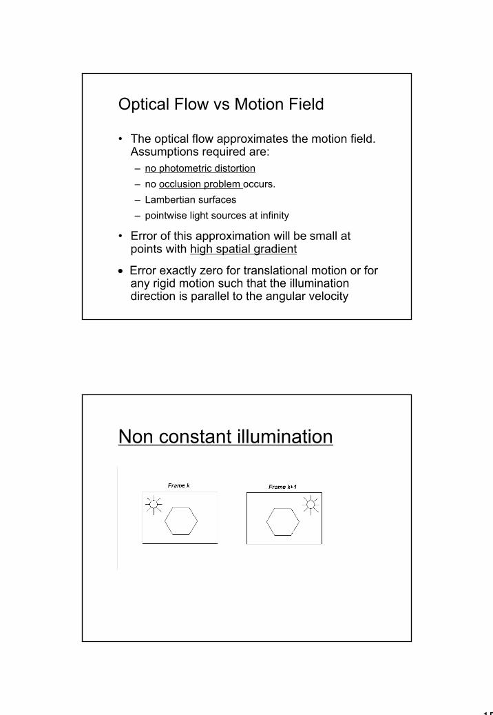
Non constant illumination

16

Occlusion Problem

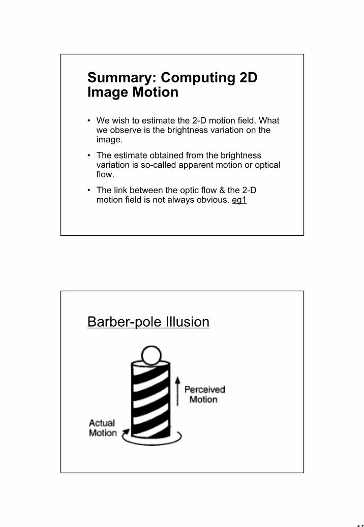
•It is impossible to find correspondence in the to be covered anduncovered regions. An example: Barber-pole illusion.

•Thus strictly speaking, the motion field estimates are accurate only if the changes in intensity over time are due to texture and surface markings on the moving surfaces, rather than depth discontinuities occluding each other.

Barber-pole Illusion

A. Barberpole Illusion B. Possible Motions in the Center C. Possible Motion at the Edge

If the stripes were made up of many red dots on a white background so that correspondences over time were unambiguous, the barberpole illusion should disappear.

Notice that the ends of the stripes at the bottom edge of the barberpole are actually moving leftward. Because they are true endpoints, they specify the true motion of the pole.

Why do these bottom endpoints not determine the perceived motion of the whole barberpole? The answer appears to be that they are simply overwhelmed by the larger number of ends along the sides.If the barber-pole is fat and short (so that there are less endpoints), then the perceived motion is horizontal!

17

Insufficient spatial image gradient

Flow vs Correspondence

• Gradient based methods only work when the 2D motion is ``small'' so that the derivatives can be reliably computed -- example of large “motion”: stereo pair, action movie.-- to cope with ``large'' 2D motions, one has to employ

multiresolution methods

• Preferably, correspondence algorithms should be used to compute 2D motion when the motion is “large'‘. -- correlation -- feature tracking

18

Summary: Computing 2D Image Motion

• We wish to estimate the 2-D motion field. What we observe is the brightness variation on the image.

• The estimate obtained from the brightness variation is so-called apparent motion or optical flow.

• The link between the optic flow & the 2-D motion field is not always obvious. eg1

Barber-pole Illusion

19

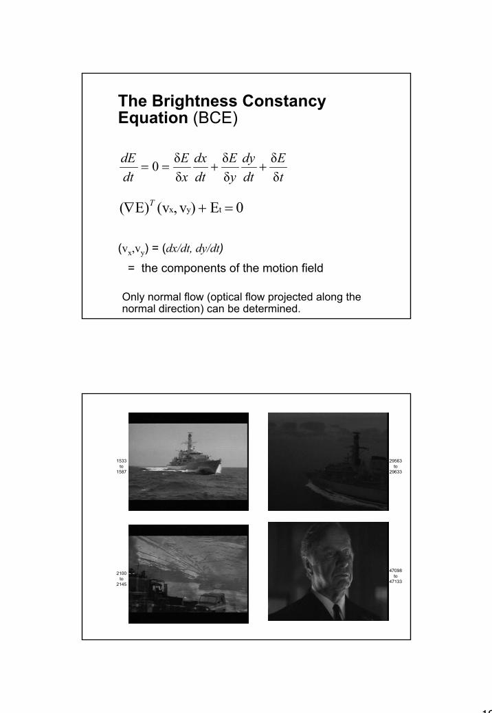
The Brightness Constancy Equation (BCE)

(vx,vy) = (dx/dt, dy/dt)

= the components of the motion field

tE

dtdy

yE

dtdx

xE

dtdE

δδ

δδ

δδ0 ++==

0 E )v,(vE)( tyx =+∇ T

Only normal flow (optical flow projected along the normal direction) can be determined.

1533to

1587

2100to

2145

29563to

29633

47098to

47133

20

3746to

3764

3764to

3777

48682to

48708

48998to

49018

End of 2D Motion Estimation

Reference:

- Chapter 8, Textbook

- Handout (Motion and Depth Perception)