Embed Size (px)
Citation preview
Should we abandon the t-test ? A statistical comparison of 8 differential gene expression tests
Marine Jeanmougin, Master student INSA-Lyon
Mickaël Guedj1,3, Grégory Nuel2,3
1. Ligue Nationale contre le Cancer – Cartes d’Identité des Tumeurs program (CIT)
2. Paris Descartes University – MAP5 laboratory
3. Statistics for Systems Biology working group
SMPGD’09
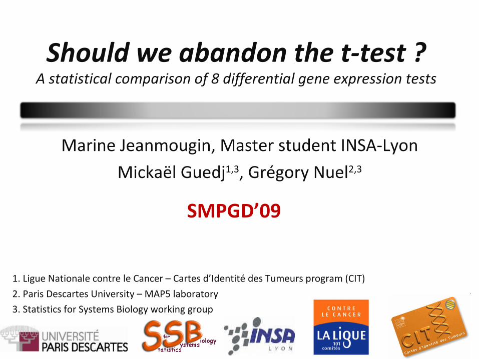
Analysis process
Differential analysis
Experiment Pre-processing
(normalization…)
Post-analysis (classification, multiple- testing, prediction…)
microarray data
Normalized microarraydata
Differentially expressed gene lists
2
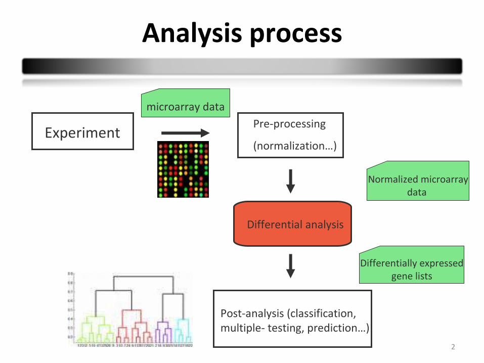
Hypothesis testing
Differential analysis : comparison of 2 populations (or more) according to a variable of interest (expression level).
Statistical hypothesis : assumption about a population parameter :2 types of statistical hypotheses :
H0 : Expression level is the same between the 2 populations
H1 : Expression level differs between the 2 populations
3
4
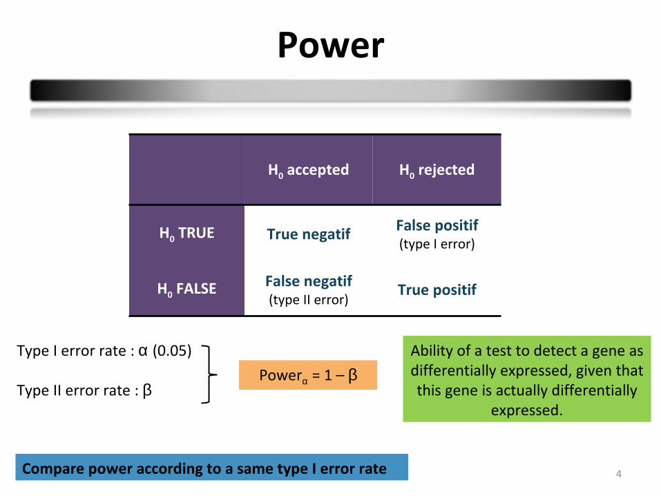
Power
H0 accepted H0 rejected
H0 TRUE True negatif False positif(type I error)
H0 FALSE False negatif(type II error)
True positif
Type I error rate : α (0.05)
Type II error rate : βPowerα = 1 – β
Ability of a test to detect a gene as differentially expressed, given that this gene is actually differentially
expressed.
Compare power according to a same type I error rate
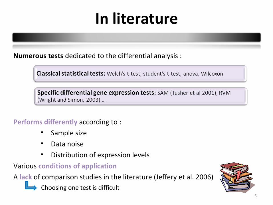
In literature
Numerous tests dedicated to the differential analysis :
5
Performs differently according to :• Sample size• Data noise• Distribution of expression levels
Various conditions of application
A lack of comparison studies in the literature (Jeffery et al. 2006)
Choosing one test is difficult
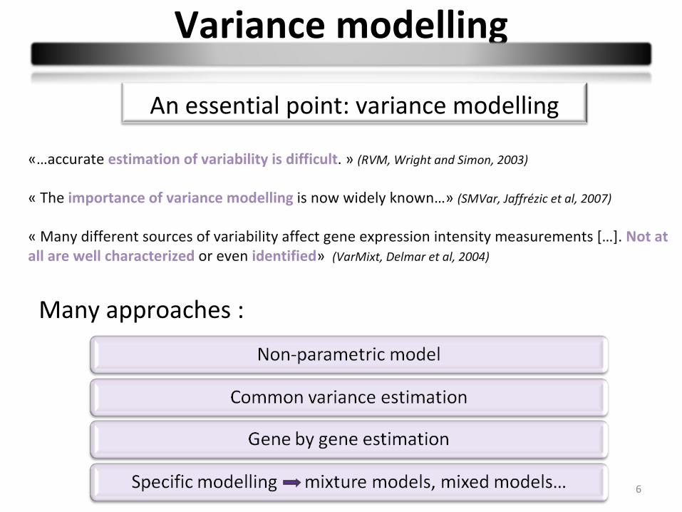
«…accurate estimation of variability is difficult. » (RVM, Wright and Simon, 2003)
« The importance of variance modelling is now widely known…» (SMVar, Jaffrézic et al, 2007)
« Many different sources of variability affect gene expression intensity measurements […]. Not at all are well characterized or even identified» (VarMixt, Delmar et al, 2004)
Variance modelling
An essential point: variance modelling
6
Many approaches :
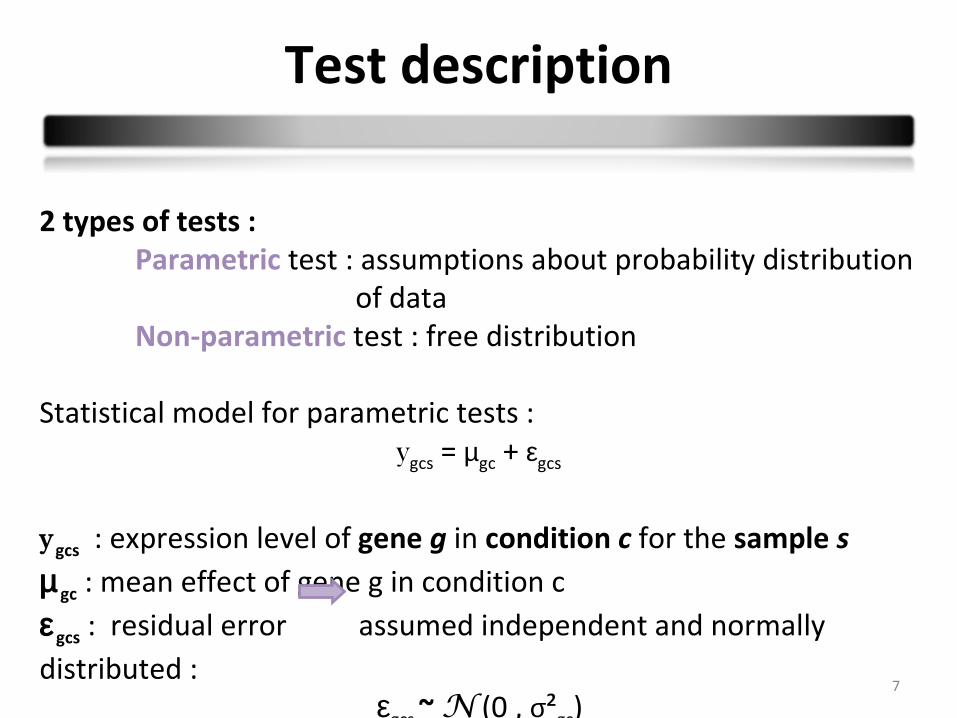
Test description
2 types of tests :Parametric test : assumptions about probability distribution
of dataNon-parametric test : free distribution
Statistical model for parametric tests : ygcs = µgc + εgcs
y gcs : expression level of gene g in condition c for the sample sµgc : mean effect of gene g in condition cε gcs : residual error assumed independent and normally distributed :
εgcs ~ N (0 , σ²gc) 7
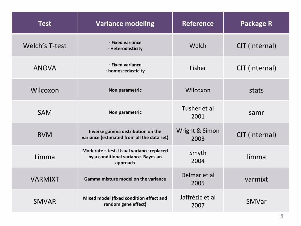
Test Variance modeling Reference Package R
Welch’s T-test - Fixed variance- Heterodasticity Welch CIT (internal)
ANOVA - Fixed variance- homoscedasticity Fisher CIT (internal)
Wilcoxon Non parametric Wilcoxon stats
SAM Non parametricTusher et al
2001 samr
RVM Inverse gamma distribution on the variance (estimated from all the data set)
Wright & Simon2003 CIT (internal)
LimmaModerate t-test. Usual variance replaced
by a conditional variance. Bayesian approach
Smyth2004 limma
VARMIXT Gamma mixture model on the varianceDelmar et al
2005 varmixt
SMVAR Mixed model (fixed condition effect and random gene effect)
Jaffrézic et al 2007 SMVar
8
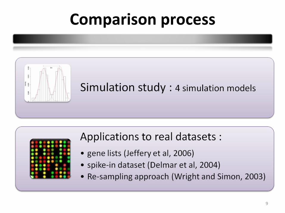
Comparison process
9
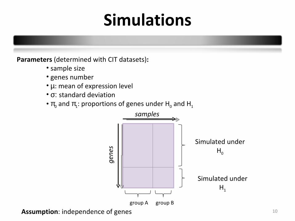
Simulations
10
Parameters (determined with CIT datasets):• sample size• genes number• µ: mean of expression level• σ: standard deviation• π0 and π1: proportions of genes under H0 and H1
Simulated underH0
Simulated underH1
gene
ssamples
group B group A
Assumption: independence of genes
Simulations
11
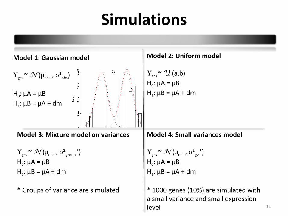
Model 1: Gaussian model
Ygcs ~ N (µobs , σ²obs)
H0: µA = µBH1: µB = µA + dm
Model 2: Uniform model
Ygcs ~ U (a,b)H0: µA = µB H1: µB = µA + dm
Model 3: Mixture model on variances
Ygcs ~ N (µobs , σ²group *)
H0: µA = µB H1: µB = µA + dm
* Groups of variance are simulated
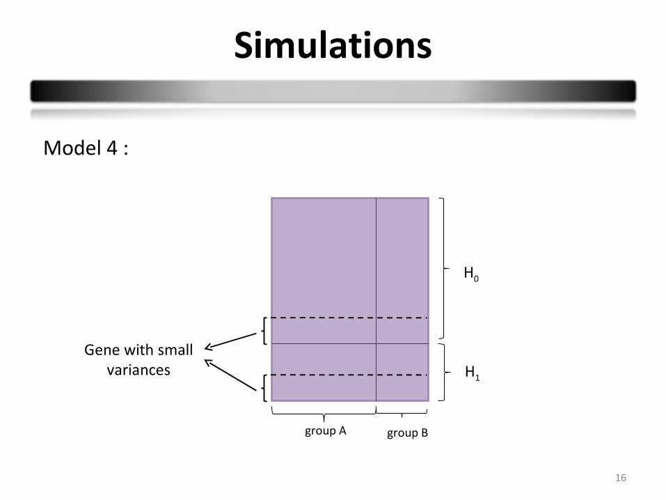
Model 4: Small variances model
Ygcs ~ N (µobs , σ²gv *)
H0: µA = µB H1: µB = µA + dm
* 1000 genes (10%) are simulated with a small variance and small expression level
Simulations
12
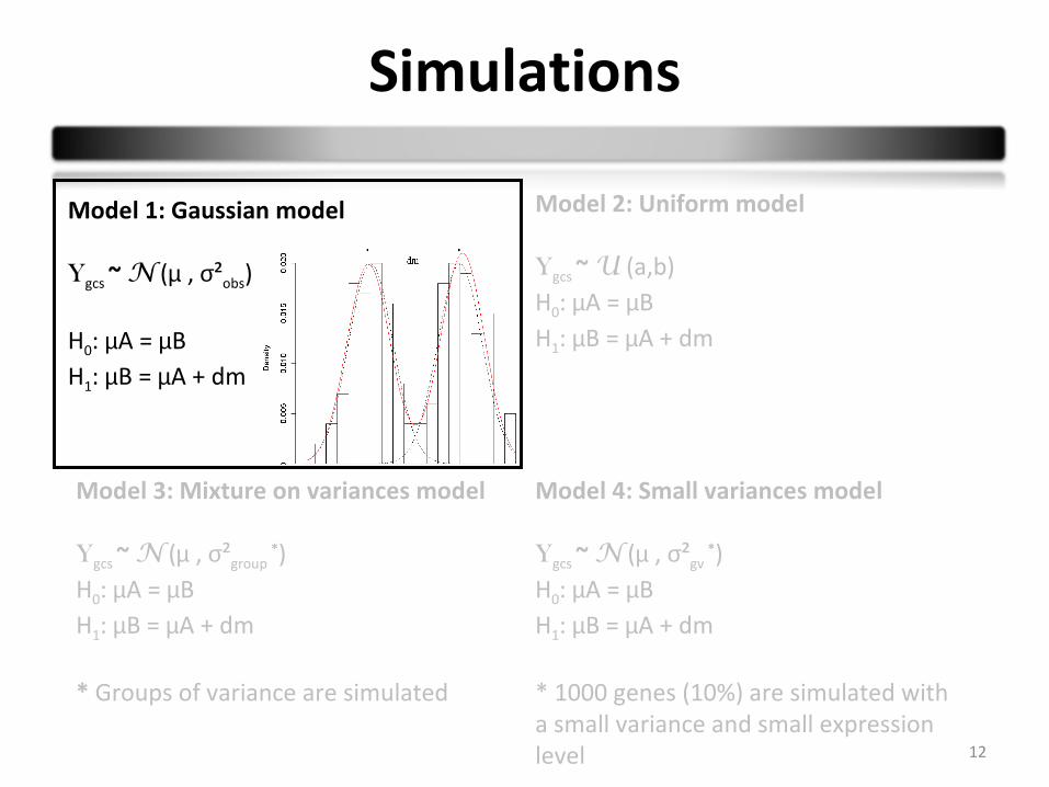
Model 1: Gaussian model
Ygcs ~ N (µ , σ²obs)
H0: µA = µB H1: µB = µA + dm
Model 2: Uniform model
Ygcs ~ U (a,b)H0: µA = µB H1: µB = µA + dm
Model 3: Mixture on variances model
Ygcs ~ N (µ , σ²group *)
H0: µA = µB H1: µB = µA + dm
* Groups of variance are simulated
Model 4: Small variances model
Ygcs ~ N (µ , σ²gv *)
H0: µA = µB H1: µB = µA + dm
* 1000 genes (10%) are simulated with a small variance and small expression level
Simulations
13
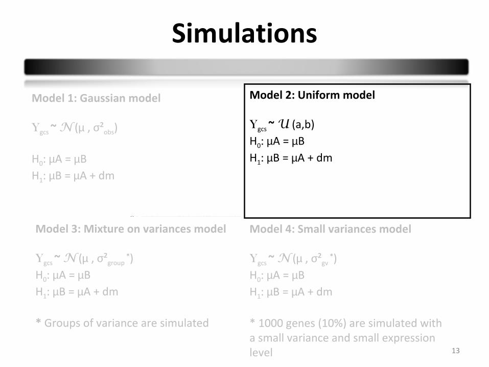
Model 1: Gaussian model
Ygcs ~ N (µ , σ²obs)
H0: µA = µB H1: µB = µA + dm
Model 2: Uniform model
Ygcs ~ U (a,b)H0: µA = µB H1: µB = µA + dm
Model 3: Mixture on variances model
Ygcs ~ N (µ , σ²group *)
H0: µA = µB H1: µB = µA + dm
* Groups of variance are simulated
Model 4: Small variances model
Ygcs ~ N (µ , σ²gv *)
H0: µA = µB H1: µB = µA + dm
* 1000 genes (10%) are simulated with a small variance and small expression level
Simulations
14
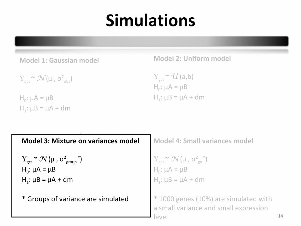
Model 1: Gaussian model
Ygcs ~ N (µ , σ²obs)
H0: µA = µB H1: µB = µA + dm
Model 2: Uniform model
Ygcs ~ U (a,b)H0: µA = µB H1: µB = µA + dm
Model 3: Mixture on variances model
Ygcs ~ N (µ , σ²group *)
H0: µA = µB H1: µB = µA + dm
* Groups of variance are simulated
Model 4: Small variances model
Ygcs ~ N (µ , σ²gv *)
H0: µA = µB H1: µB = µA + dm
* 1000 genes (10%) are simulated with a small variance and small expression level
Simulations
15
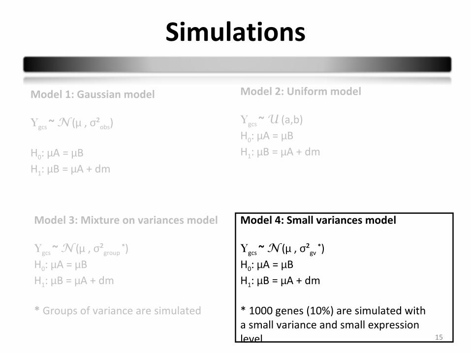
Model 1: Gaussian model
Ygcs ~ N (µ , σ²obs)
H0: µA = µB H1: µB = µA + dm
Model 2: Uniform model
Ygcs ~ U (a,b)H0: µA = µB H1: µB = µA + dm
Model 3: Mixture on variances model
Ygcs ~ N (µ , σ²group *)
H0: µA = µB H1: µB = µA + dm
* Groups of variance are simulated
Model 4: Small variances model
Ygcs ~ N (µ , σ²gv *)
H0: µA = µB H1: µB = µA + dm
* 1000 genes (10%) are simulated with a small variance and small expression level
Simulations
16
group A group B
H0
H1
Gene with small variances
Model 4 :
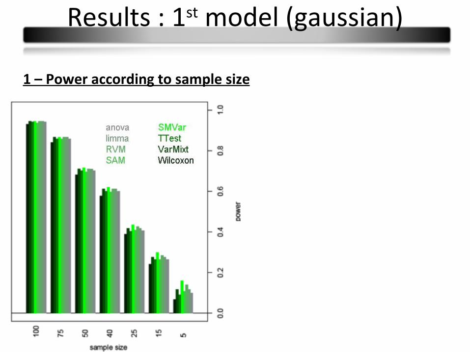
1 – Power according to sample size
Results : 1st model (gaussian)

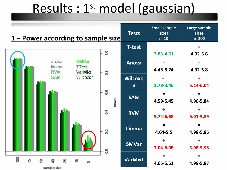
1 – Power according to sample size
Results : 1st model (gaussian)
1 – Power according to sample size
Results : 1st model (gaussian)
TestsSmall sample
sizesn=10
Large sample sizes
n=200
T-test -
3.83-4.61
=
4.92-5.8
Anova =
4.46-5.24
=
4.92-5.8
Wilcoxon
-
2.78-3.46
+
5.14-6.04
SAM=
4.59-5.45
=
4.96-5.84
RVM+
5.74-6.68
+
5.01-5.89
Limma=
4.64-5.5
=
4.98-5.86
SMVar+
7.04-8.08
+
5.08-5.98
VarMixt=
4.65-5.51
=
4.99-5.87
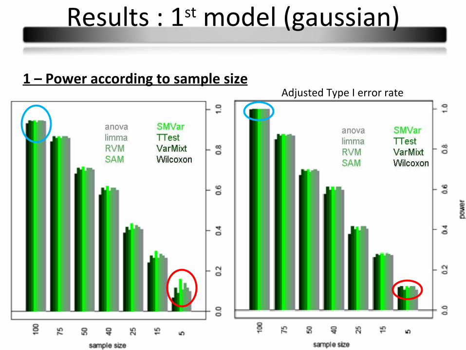
1 – Power according to sample sizeAdjusted Type I error rate
Results : 1st model (gaussian)
Results : 1st model (gaussian)
21
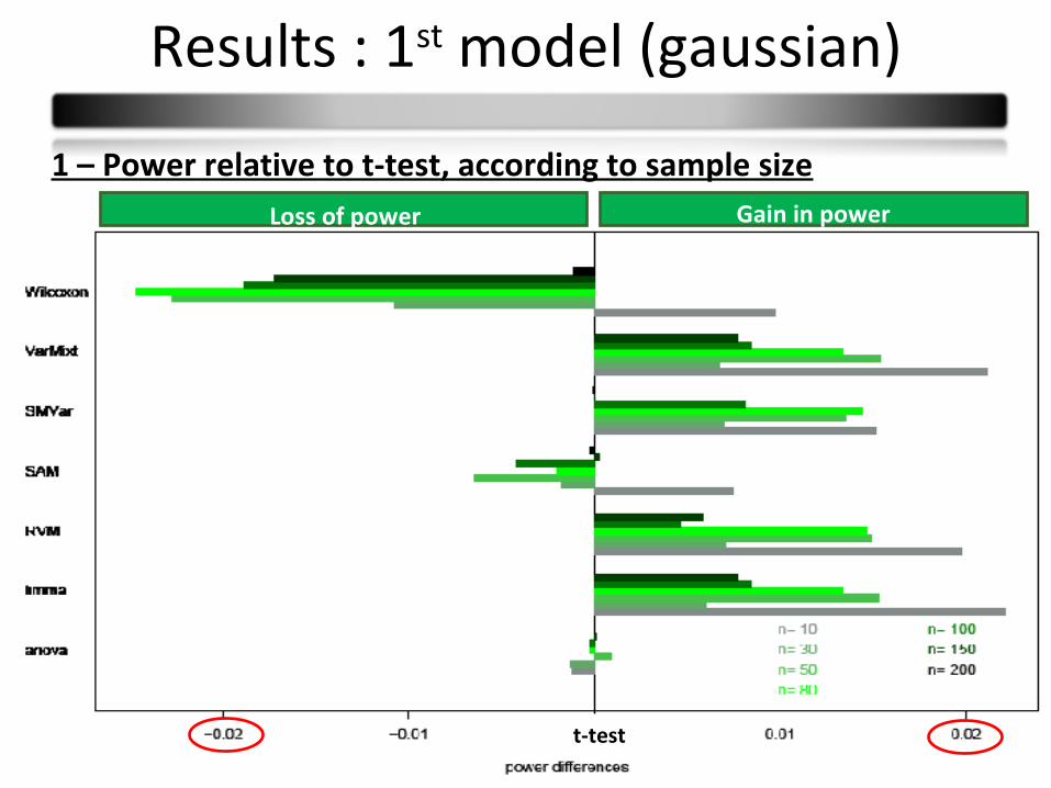
1 – Power relative to t-test, according to sample sizeGain in powerLoss of power
t-test
Results : 1st model (gaussian)
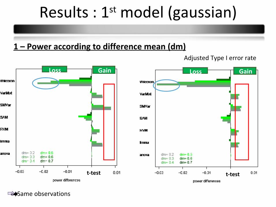
1 – Power according to difference mean (dm)Adjusted Type I error rate
GainLoss
t-test t-test
GainLoss
Same observations
Results : 1st model (gaussian)
Conclusions :
Few power differences
Observed differences in small sample sizes partly due to type I error rates
Wilcoxon: less powerful
Limma and varmixt : similar good results
Anova : equivalent to the t-test
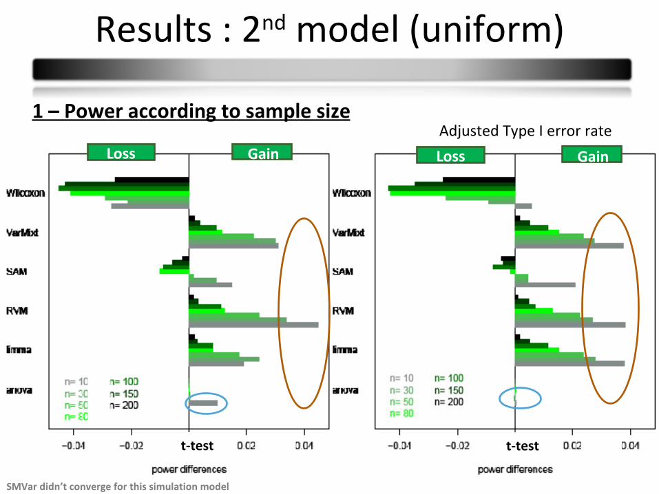
Results : 2nd model (uniform)
1 – Power according to sample sizeAdjusted Type I error rate
SMVar didn’t converge for this simulation model
GainLoss GainLoss
t-testt-test
Results
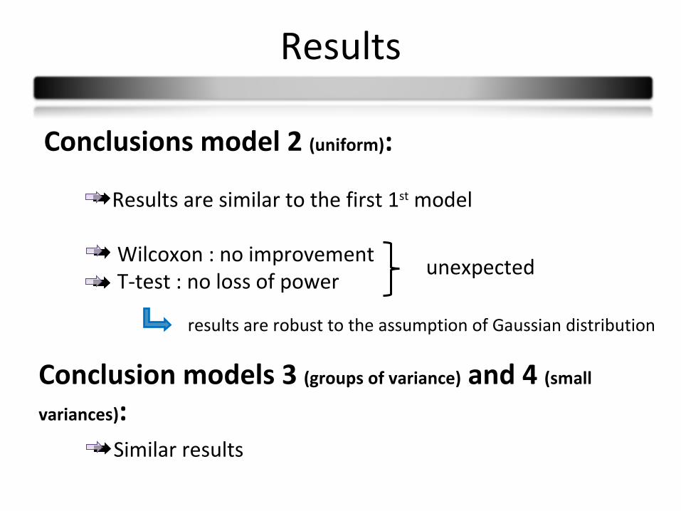
Conclusions model 2 (uniform):
Results are similar to the first 1st model
Wilcoxon : no improvement T-test : no loss of power
Conclusion models 3 (groups of variance) and 4 (small
variances): Similar results
unexpected
results are robust to the assumption of Gaussian distribution
26
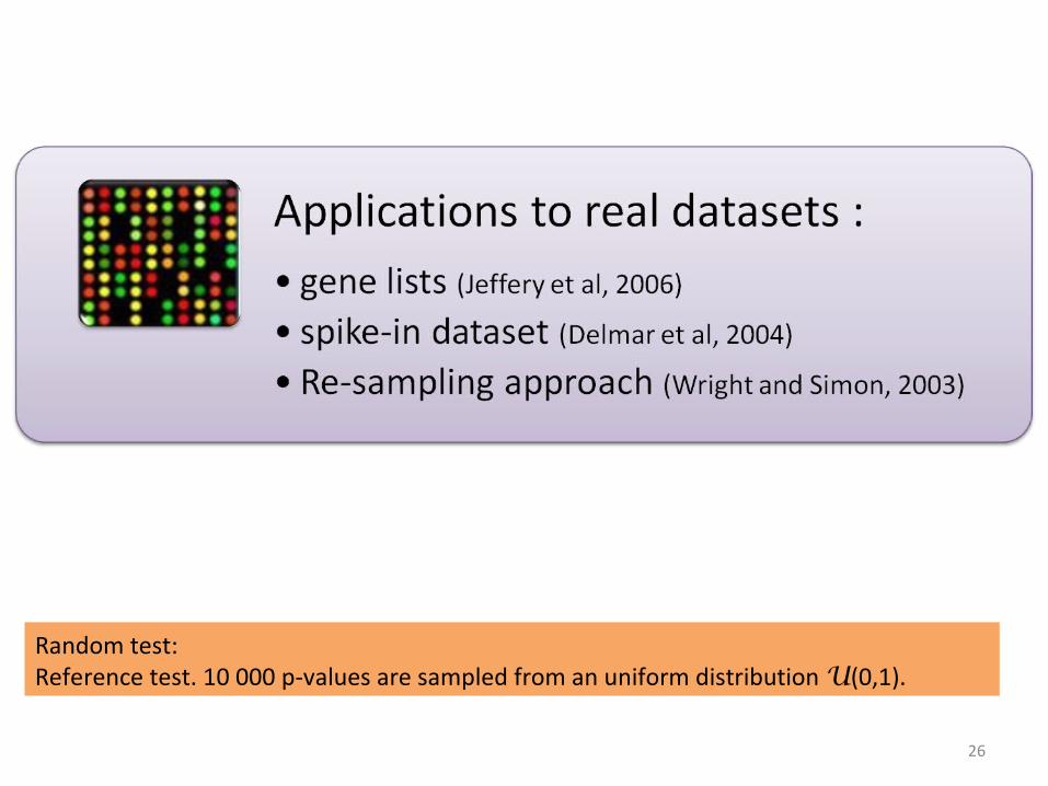
Random test:Reference test. 10 000 p-values are sampled from an uniform distribution U(0,1).
27
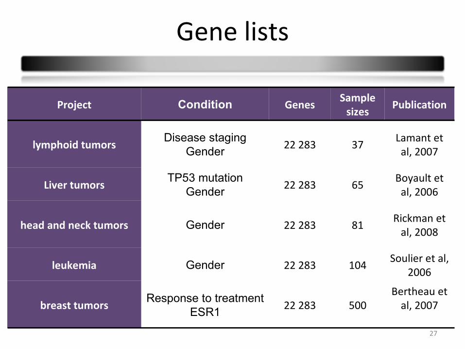
Gene lists
Project Condition GenesSample
sizesPublication
lymphoid tumorsDisease staging
Gender22 283 37
Lamant et al, 2007
Liver tumorsTP53 mutation
Gender22 283 65
Boyault et al, 2006
head and neck tumors Gender 22 283 81Rickman et
al, 2008
leukemia Gender 22 283 104Soulier et al,
2006
breast tumorsResponse to treatment
ESR122 283 500
Bertheau et al, 2007
28
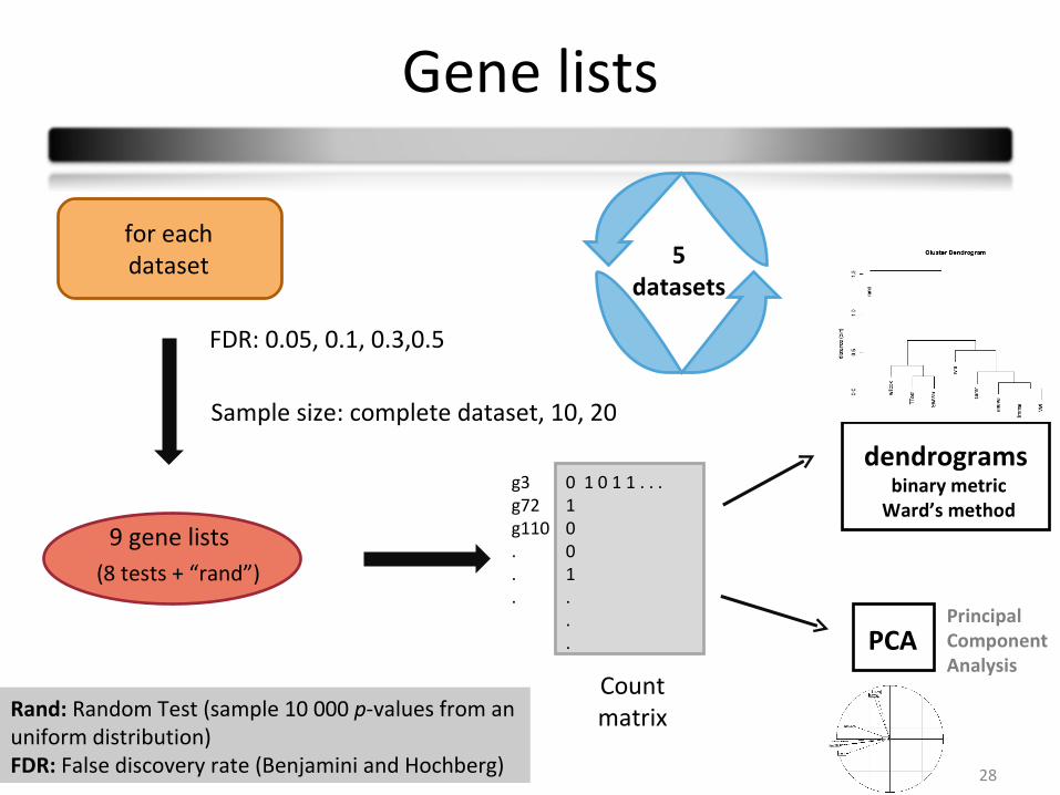
Gene lists
for eachdataset
9 gene lists
Countmatrix
g3g72g110...
0 1 0 1 1 . . . 1001...
dendrogramsbinary metric
Ward’s method
PCA
(8 tests + “rand”)
FDR: 0.05, 0.1, 0.3,0.5
5 datasets
Sample size: complete dataset, 10, 20
Rand: Random Test (sample 10 000 p-values from an uniform distribution)FDR: False discovery rate (Benjamini and Hochberg)
PrincipalComponentAnalysis
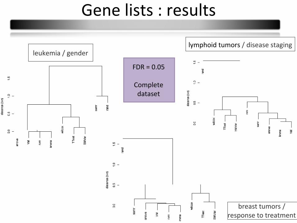
Gene lists : results
breast tumors / response to treatment
leukemia / genderlymphoid tumors / disease staging
FDR = 0.05
Complete dataset
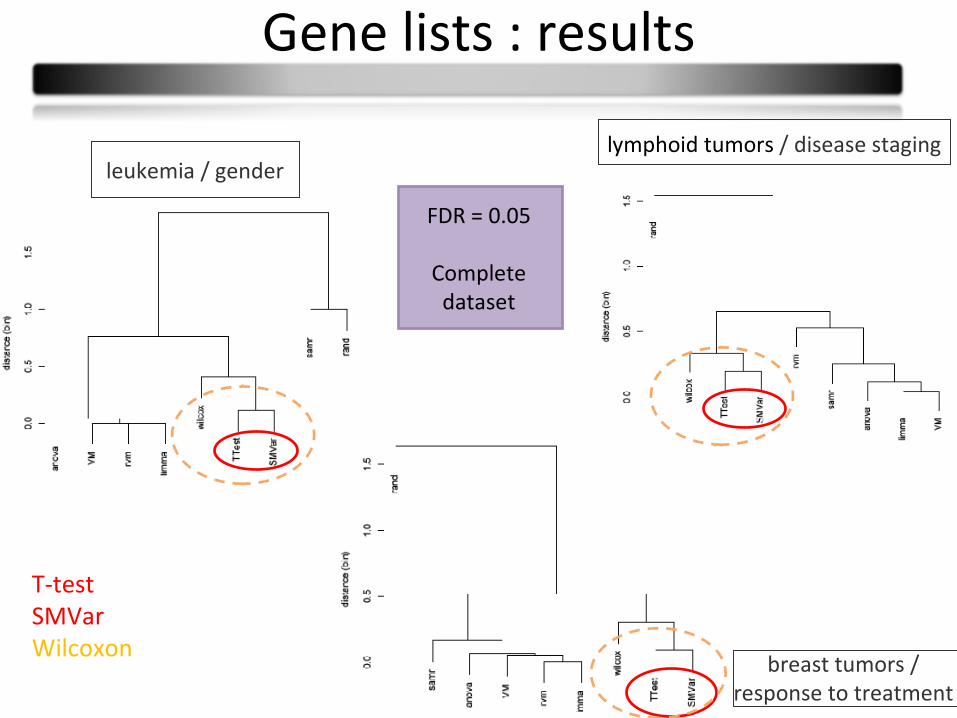
Gene lists : results
breast tumors / response to treatment
FDR = 0.05
Complete dataset
leukemia / genderlymphoid tumors / disease staging
T-testSMVarWilcoxon
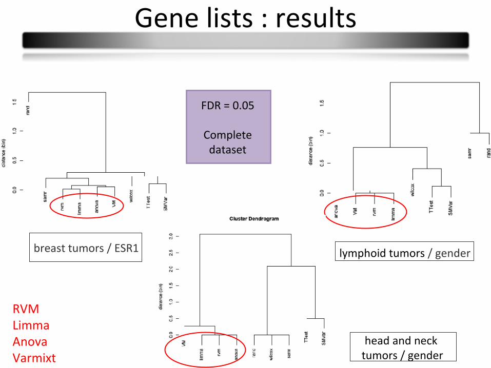
Gene lists : results
lymphoid tumors / gender
head and neck tumors / gender
breast tumors / ESR1
FDR = 0.05
Complete dataset
RVMLimmaAnovaVarmixt
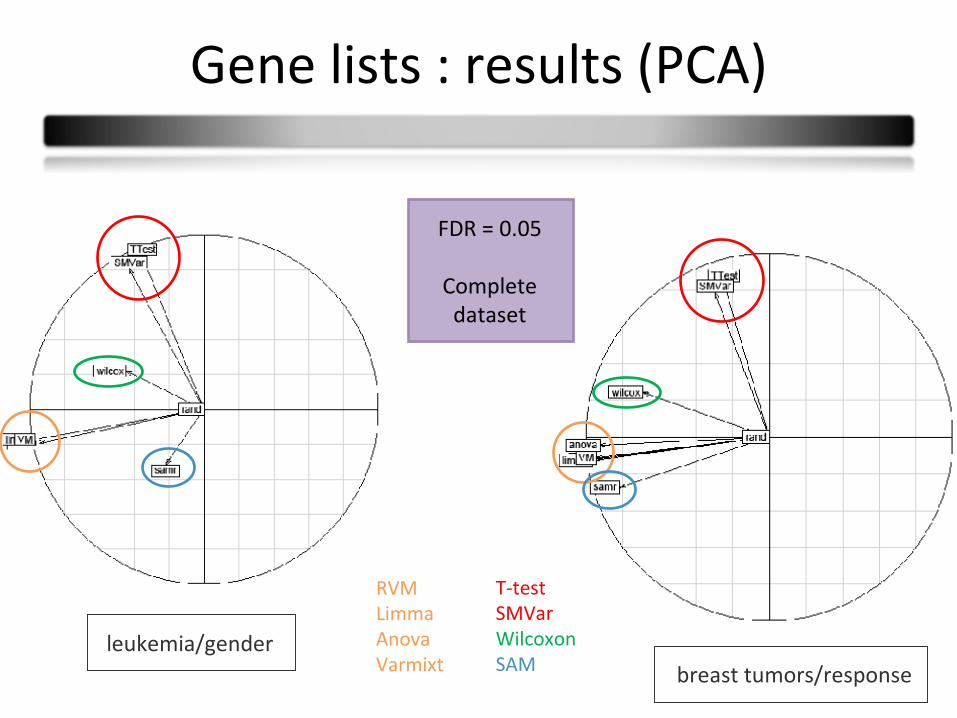
Gene lists : results (PCA)
breast tumors/responseleukemia/gender
FDR = 0.05
Complete dataset
RVMLimmaAnovaVarmixt
T-testSMVarWilcoxonSAM
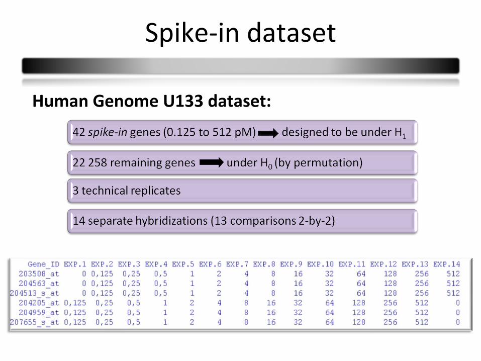
Spike-in dataset
Human Genome U133 dataset:
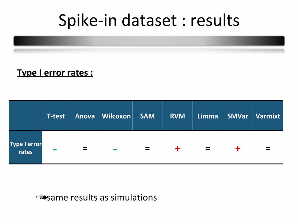
Spike-in dataset : results
Type I error rates :
T-test Anova Wilcoxon SAM RVM Limma SMVar Varmixt
Type I error rates - = - = + = + =
same results as simulations
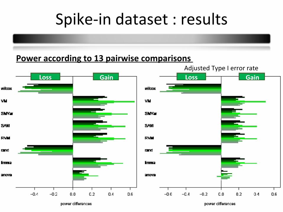
Spike-in dataset : results
Power according to 13 pairwise comparisons Adjusted Type I error rate
GainLoss GainLoss
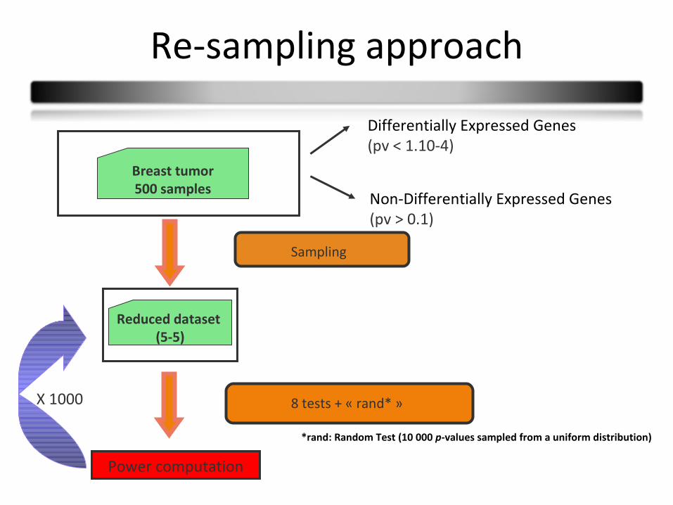
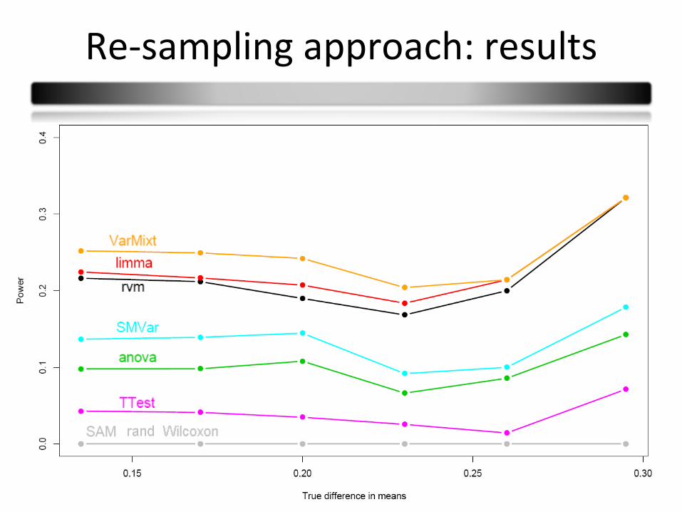
Re-sampling approach
Differentially Expressed Genes (pv < 1.10-4)
Reduced dataset (5-5)
Breast tumor500 samples
Power computation
X 1000 8 tests + « rand* »
Sampling
*rand: Random Test (10 000 p-values sampled from a uniform distribution)
Non-Differentially Expressed Genes (pv > 0.1)
37
Re-sampling approach: results
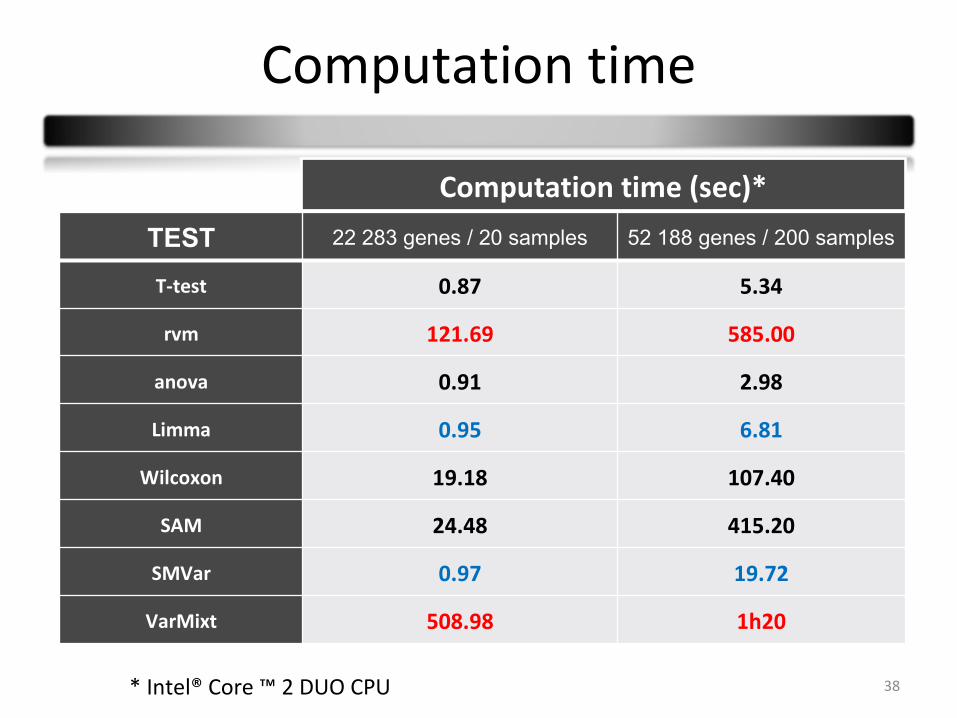
Computation time
38
TEST 22 283 genes / 20 samples 52 188 genes / 200 samples
T-test 0.87 5.34
rvm 121.69 585.00
anova 0.91 2.98
Limma 0.95 6.81
Wilcoxon 19.18 107.40
SAM 24.48 415.20
SMVar 0.97 19.72
VarMixt 508.98 1h20
* Intel® Core ™ 2 DUO CPU
Computation time (sec)*
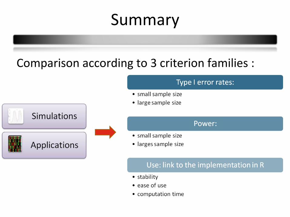
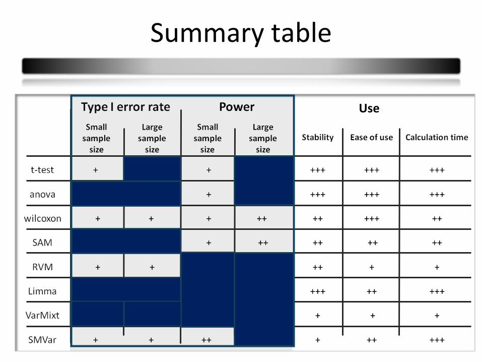
Summary
Comparison according to 3 criterion families :
40
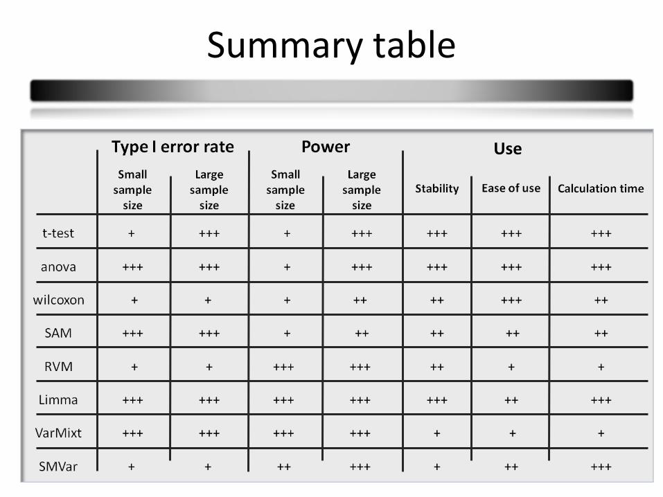
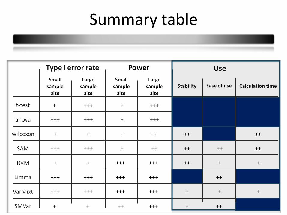
Summary table
Use
41
Summary table
41
Use
42
Summary table
42
Use
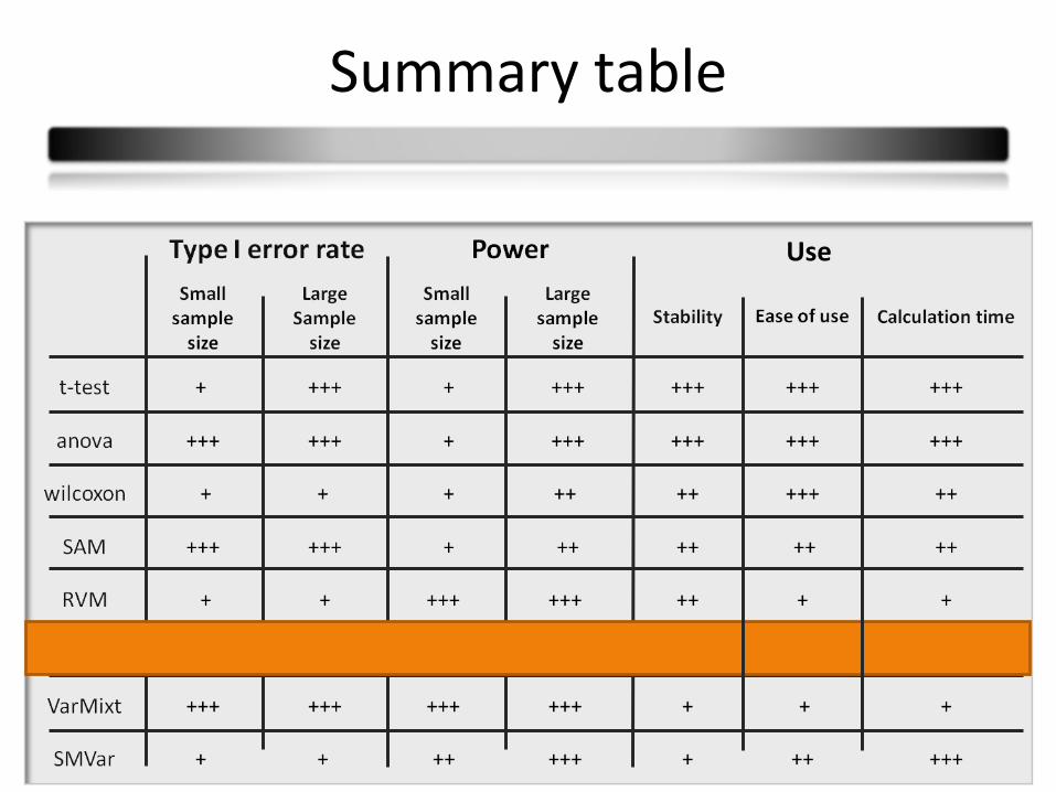
43
Summary table
4343
Use
44
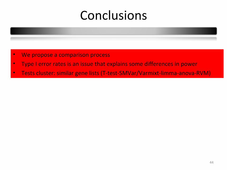
Conclusions
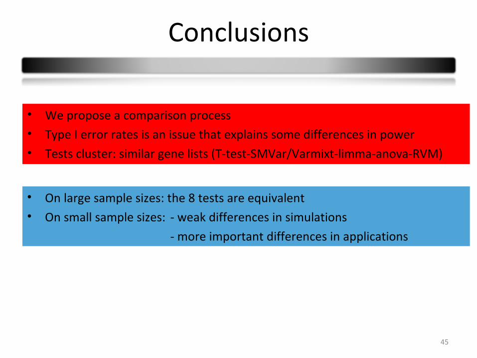
• We propose a comparison process• Type I error rates is an issue that explains some differences in power• Tests cluster: similar gene lists (T-test-SMVar/Varmixt-limma-anova-RVM)
45
Conclusions
• We propose a comparison process• Type I error rates is an issue that explains some differences in power• Tests cluster: similar gene lists (T-test-SMVar/Varmixt-limma-anova-RVM)
• On large sample sizes: the 8 tests are equivalent• On small sample sizes: - weak differences in simulations
- more important differences in applications
46
Conclusions
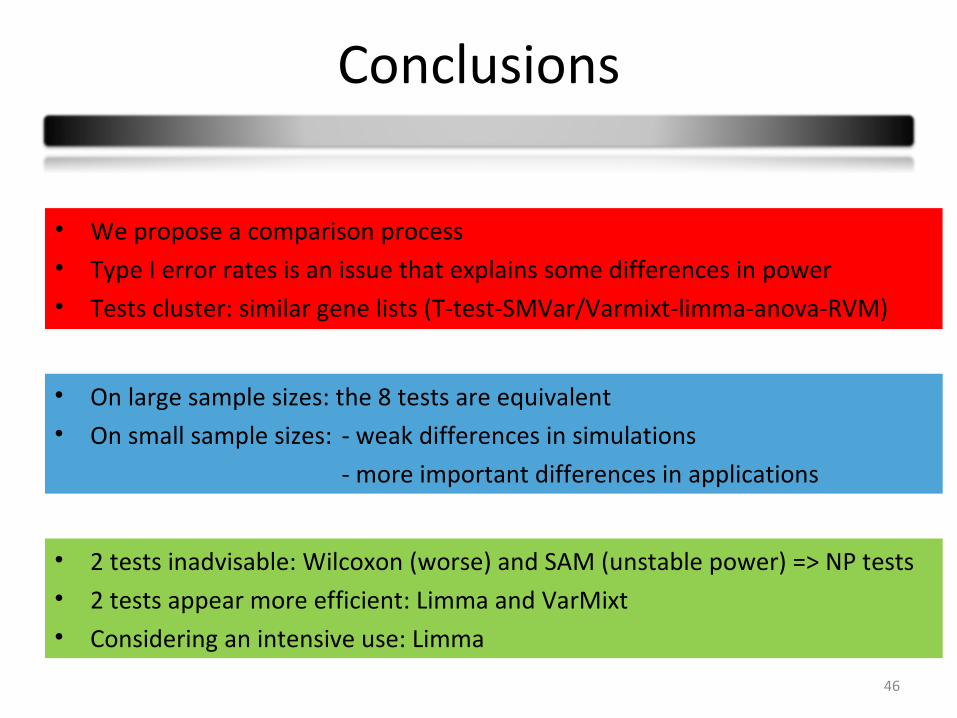
• We propose a comparison process• Type I error rates is an issue that explains some differences in power• Tests cluster: similar gene lists (T-test-SMVar/Varmixt-limma-anova-RVM)
• 2 tests inadvisable: Wilcoxon (worse) and SAM (unstable power) => NP tests• 2 tests appear more efficient: Limma and VarMixt• Considering an intensive use: Limma
• On large sample sizes: the 8 tests are equivalent• On small sample sizes: - weak differences in simulations
- more important differences in applications
Thanks
To the whole CIT’s team of the Ligue Nationale Contre le Cancer :
To M. Guedj, L. Marisa, AS. Valin, F. Petel, E. Thomas, R. Schiappa, L. Vescovo, A. de Reynies, J. Metral and J. Godet
To G. Nuel, MAP5 laboratory, UMR 8145, Paris V Universityand V. Dumeaux, Tromsø University et Paris V University
To the IRISA of Rennes
To the SMPGD’s team who enables me to introduce my work