SELECTION AND REPRESENTATION OF ATTRIBUTES FORSOFTWARE DEFECT PREDICTION

SADIA SHARMINBSSE 0426

A ThesisSubmitted to the Bachelor of Science in Software Engineering Program Office

of the Institute of Information Technology, University of Dhakain Partial Fulfillment of theRequirements for the Degree

BACHELOR OF SCIENCE IN SOFTWARE ENGINEERING

Institute of Information TechnologyUniversity of Dhaka

DHAKA, BANGLADESH

c© SADIA SHARMIN, 2015

SELECTION AND REPRESENTATION OF ATTRIBUTES FOR SOFTWAREDEFECT PREDICTION

SADIA SHARMIN

Approved:

Signature Date

Supervisor: Dr. Mohammad Shoyaib

Committee Member: Dr. Kazi Muheymin-Us-Sakib

Committee Member: Dr. Md. Shariful Islam

Committee Member: Alim Ul Gias

Committee Member: Amit Seal Ami

ii

Abstract

For software quality assurance, software defect prediction (SDP) has drawn a great

deal of attention in recent years. Its goal is to reduce verification cost, time and

effort by predicting the defective modules efficiently. The datasets used in SDP

consist of attributes which are not equally important for predicting the defects of

software. Therefore, proper attribute selection plays a significant role in building

an acceptable defect prediction model. However, selection of proper attributes

and their representation in an efficient way are very challenging because except

few basic attributes most of them are derived attributes and their reliability are

still debatable.

To address these issues, we introduce Selection of Attribute with Log filtering

(SAL) to represent them in an organized way and to select the proper set of

attributes. Our proposed attribute selection process can effectively select the best

set of attributes, which are relevant for the discrimination of defected and non-

defected software modules. We have evaluated the proposed attribute selection

method using several widely used publicly available datasets. To validate our

model, we calculate the prediction performances using some of the commonly

used measurement scales such as balance, AUC (Area Under the ROC Curve).

The simulation results demonstrate that our method is more effective to improve

the accuracy of SDP than the existing state-of-the-art methods.

iii

Acknowledgments

I would like to thank my supervisor, Dr. Mohammad Shoyaib, Associate Profes-

sor of Institute of Information Technology (IIT) for his support, motivation and

suggestion during this thesis completion. With the help of his guidance I have

been able to bring the best out of me.

iv

Publications

The publications made during the course of this research have been listed below:-

1. Sadia Sharmin, Md Rifat Arefin, M. Abdullah-Al Wadud, Naushin Nower,

Mohammad Shoyaib, SAL: An Effective Method for Software Defect Pre-

diction, The 18th International Conference on Computer and Information

Technology (ICCIT), 2015. (Accepted)

2. Md. Habibur Rahman, Sadia Sharmin, Sheikh Muhammad Sarwar, Shah

Mostafa Khaled, Mohammad Shoyaib, Software Defect Prediction using

minimized attributes. Journal of Engineering and Technology (JET), IUT,

Dhaka, Bangladesh,2015.

v

Contents

Approval ii

Abstract iii

Acknowledgements iv

Publications v

Table of Contents vi

List of Tables viii

List of Figures ix

1 Introduction 11.1 Motivation . . . . . . . . . . . . . . . . . . . . . . . . . . . . . . . . 11.2 Objectives . . . . . . . . . . . . . . . . . . . . . . . . . . . . . . . . 31.3 Organization of the Thesis . . . . . . . . . . . . . . . . . . . . . . . 3

2 Background Study 52.1 Software Defect Prediction Model . . . . . . . . . . . . . . . . . . . 52.2 Evaluation Measurement Scales . . . . . . . . . . . . . . . . . . . . 62.3 Defect Prediction Metrics . . . . . . . . . . . . . . . . . . . . . . . 92.4 Defect Prediction Dataset . . . . . . . . . . . . . . . . . . . . . . . 112.5 Defect Prediction Classifiers . . . . . . . . . . . . . . . . . . . . . . 122.6 Summary . . . . . . . . . . . . . . . . . . . . . . . . . . . . . . . . 15

3 Literature Review of Software Defect Prediction 163.1 Pre-processing . . . . . . . . . . . . . . . . . . . . . . . . . . . . . . 173.2 Attribute Selection . . . . . . . . . . . . . . . . . . . . . . . . . . . 183.3 Classification . . . . . . . . . . . . . . . . . . . . . . . . . . . . . . 203.4 Summary . . . . . . . . . . . . . . . . . . . . . . . . . . . . . . . . 21

4 Methodology 224.1 Data Pre-processing . . . . . . . . . . . . . . . . . . . . . . . . . . 224.2 Attribute Selection . . . . . . . . . . . . . . . . . . . . . . . . . . . 23

4.2.1 Ranking of Attributes . . . . . . . . . . . . . . . . . . . . . 234.2.2 Selection of the Best Set of Attributes . . . . . . . . . . . . 24

vi

4.3 Classification . . . . . . . . . . . . . . . . . . . . . . . . . . . . . . 254.4 Summary . . . . . . . . . . . . . . . . . . . . . . . . . . . . . . . . 25

5 Results 265.1 Evaluation Metrics . . . . . . . . . . . . . . . . . . . . . . . . . . . 265.2 Implementation Details . . . . . . . . . . . . . . . . . . . . . . . . . 275.3 Results and Discussions . . . . . . . . . . . . . . . . . . . . . . . . 275.4 Summary . . . . . . . . . . . . . . . . . . . . . . . . . . . . . . . . 29

6 Conclusion 31

Bibliography 33

vii

List of Tables

2.1 Confusion Matrix for Machine Learning . . . . . . . . . . . . . . . . 62.2 Software Code Attributes of Defect Prediction . . . . . . . . . . . . 92.3 NASA Dataset Overview . . . . . . . . . . . . . . . . . . . . . . . . 11

5.1 Comparison of Balance Values of Different Defect Prediction Meth-ods . . . . . . . . . . . . . . . . . . . . . . . . . . . . . . . . . . . 28

5.2 Comparison of AUC Values of Different Defect Prediction Methods 295.3 Comparison of AUC Values of Different Classifiers using SAL . . . 30

viii

List of Figures

4.1 An Overview of Software Defect Prediction Process . . . . . . . . . 224.2 An Overview of Attribute Selection Process . . . . . . . . . . . . . 23

5.1 Performance of Log-filtering for Different ∈ Values . . . . . . . . . . 27

ix

Chapter 1

Introduction

In software development life-cycle, software testing is regarded as one of most

significant processes. In this stage, we try to identify the bugs of the software in

order to meet its required quality. More than 50% of time is spent in this phase

for maintaining the reliability and quality of software. It can be viewed as trade-

off of time, budget and quality. However, finding errors in the program modules

is not an easy task to perform. As a result, many defect prediction techniques

have been introduced approaching this problem. It has become an integral part of

testing phase. A lot of researches have been undergoing for building a good defect

prediction technique in order to predict the defective modules in an efficient way.

1.1 Motivation

In recent years, software defect prediction (SDP) has become an important re-

search topic in the field of software industry. SDP is the way to estimate the

location of the bugs of the software after being developed so that the quality and

the productivity can be improved.

The historical datasets collected during software development phase consist

of the data about software based on some software metrics like line of code, cy-

clomatic complexity, essential complexity, total operators and operands etc. This

1

attributes are regarded as the measurement of software. By using these attributes,

we can predict which components are more likely to be defect-prone as compared

to the others. The performance of a defect prediction model is usually significantly

influenced by the characteristics of the attributes [1]. However, a set of standard

attributes has not yet been agreed that can be used for defect prediction. It is

found that the attributes of different datasets used for SDP are not same. All

of them are not even necessary for defect prediction [2]. Rather, some attributes

might decrease the performance of defect prediction models. In contrast, some

are highly responsible. Performance of these models increases if we remove these

irrelevant and unnecessary attributes [1, 3, 4]. Therefore, one of the main con-

cerns is to remove the unnecessary or irrelevant attributes from the set of available

attributes so that the minimized set can lead to a faster model training [4].

Apart from attribute selection, pre-processing of data also improves the classi-

fication performance. The training data sets are pre-processed to remove outliers,

handle missing value, discretize or transform numeric attributes etc. which influ-

ence the prediction result [5]. The overall performance of defect prediction can be

realized by the combination of an effective attribute selection method augmented

by a suitable normalization technique.

Classifiers are used to discriminate the non-defect modules from the defective

ones by using a prediction model derived from the training data-sets. A variety

of learning algorithms have been applied as classifiers, but none has proven to

be consistently accurate. These classifiers include statistical algorithm, machine

learning algorithm, rules based algorithm and mixed algorithms etc. Thus, another

research area in this regard is to find an appropriate classifier for the selected

attributes to get the final decision.

2

1.2 Objectives

Various defect predication techniques have been experimented and analyzed till

now. But there is no standard model of defect prediction which will generate the

best result for identifying the bugs. Implementing a new defect prediction tech-

nique covering limitations of existing approaches or bringing some modifications

can produce better result. So, the objectives of my study are:

1. To analyze the existing pre-processing methods and find out how they can be

used with the attribute selection methods more efficiently to produce better

result.

2. To analyze the limitations of the existing methods and propose an effective

attribute selection method that will improve the accuracy of software defect

prediction.

3. To do a comparative study among the classifiers in order to find out the

appropriate one for the best set of attributes.

1.3 Organization of the Thesis

This section provides an overview about the remaining chapters of this thesis. The

chapters are organized as follows:

Chapter 2: This chapter describes the background of the thesis work describ-

ing the defect prediction models and its associated attributes, defect prediction

datasets etc.

Chapter 3: In this chapter the existing works have been discussed for defect

prediction.

Chapter 4: This chapter presents the contributions of this thesis and how it

works to improve the defect prediction accuracy. All the algorithms along with

necessary descriptions have been presented in this chapter.

3

Chapter 5: The experimental design and their results are discussed in this

chapter.

Chapter 6: This chapter concludes the thesis work giving some future direc-

tions of our work.

4

Chapter 2

Background Study

Software Defect prediction has been an active research area in software engineering

due to its positive impact on quality assurance. It provides the list of defect-prone

software modules which help the quality assurance team to allocate its limited

resource for testing and investigating the software products. The most important

fact in software defect prediction is the training and testing data set as these come

in the form of software metrics where a software code is represented as attributes

(i.e. lines of code, cyclomatic complexity, branch count etc.). Based on this

software product metrics, several publicly available dataset has been prepared to

accommodate the defect prediction purposes. In these circumstances, defect pre-

diction may be done using some of the statistical and machine learning classifiers

(i.e. Bayesian network, Logistic Regression etc.) and the performance can be eval-

uated using some of the commonly used measurement scales (i.e. balance, Area

under the ROC Curve etc.).

2.1 Software Defect Prediction Model

The first task of building a prediction model is to extract instances from software.

The software archives may be an email-archive, issue tracking system, version

control system and historical database etc. Every instances of these archive rep-

5

resent a system, a software package, a source code file, a class, a function (or

method) change according to prediction granularity. An instance contains several

attributes which are extracted from the software archive and all are labeled with

defected/no-defected or the number of bugs.

When we have instances with metrics and their corresponding labels, the next

task is to pre-process those instances which is a commonly used technique in

machine learning. Many defect prediction tasks have been conducted using the

concept of pre-processing of the dataset which includes noise reduction, attribute

selection, data normalization. When the pre-processing step is completed and we

get the final set of training instances, we can train the defect prediction model.

After that, if a new test instance needs to classify, we pass it to the defect predic-

tion model and we get a binary classification of that instances as defected or not

defected.

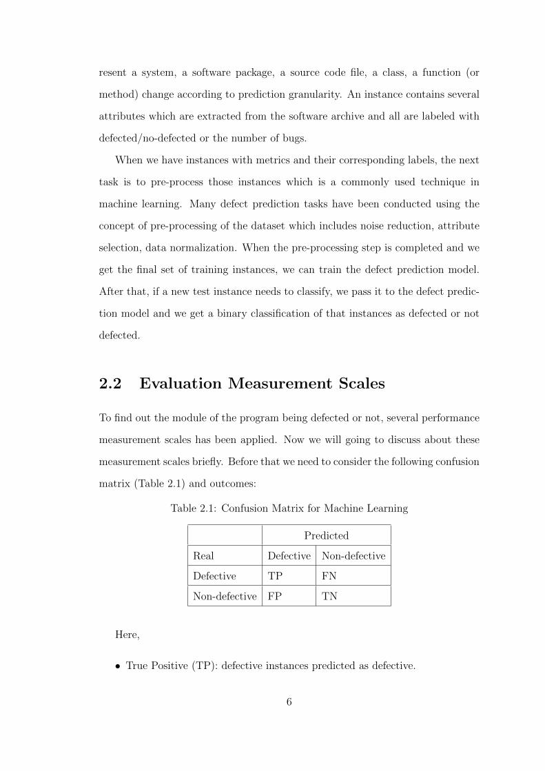
2.2 Evaluation Measurement Scales

To find out the module of the program being defected or not, several performance

measurement scales has been applied. Now we will going to discuss about these

measurement scales briefly. Before that we need to consider the following confusion

matrix (Table 2.1) and outcomes:

Table 2.1: Confusion Matrix for Machine Learning

Predicted

Real Defective Non-defective

Defective TP FN

Non-defective FP TN

Here,

• True Positive (TP): defective instances predicted as defective.

6

• False Positive (FP): Non-defective instances predicted as defective.

• True Negative (TN): Non-defective instances predicted as non-defective.

• False Negative (FN): Defective instances predicted as non-defective.

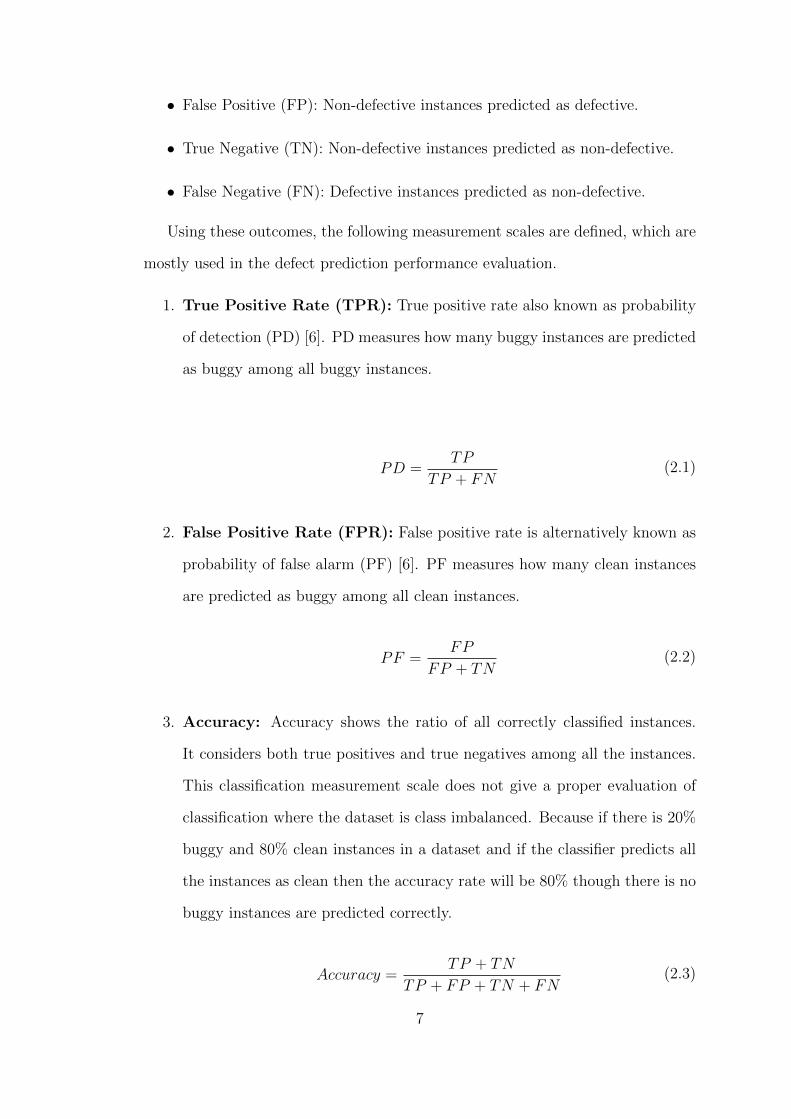
Using these outcomes, the following measurement scales are defined, which are

mostly used in the defect prediction performance evaluation.

1. True Positive Rate (TPR): True positive rate also known as probability

of detection (PD) [6]. PD measures how many buggy instances are predicted

as buggy among all buggy instances.

PD =TP

TP + FN(2.1)

2. False Positive Rate (FPR): False positive rate is alternatively known as

probability of false alarm (PF) [6]. PF measures how many clean instances

are predicted as buggy among all clean instances.

PF =FP

FP + TN(2.2)

3. Accuracy: Accuracy shows the ratio of all correctly classified instances.

It considers both true positives and true negatives among all the instances.

This classification measurement scale does not give a proper evaluation of

classification where the dataset is class imbalanced. Because if there is 20%

buggy and 80% clean instances in a dataset and if the classifier predicts all

the instances as clean then the accuracy rate will be 80% though there is no

buggy instances are predicted correctly.

Accuracy =TP + TN

TP + FP + TN + FN(2.3)

7

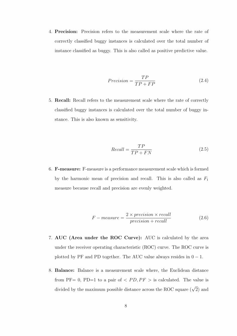
4. Precision: Precision refers to the measurement scale where the rate of

correctly classified buggy instances is calculated over the total number of

instance classified as buggy. This is also called as positive predictive value.

Precision =TP

TP + FP(2.4)

5. Recall: Recall refers to the measurement scale where the rate of correctly

classified buggy instances is calculated over the total number of buggy in-

stance. This is also known as sensitivity.

Recall =TP

TP + FN(2.5)

6. F-measure: F-measure is a performance measurement scale which is formed

by the harmonic mean of precision and recall. This is also called as F1

measure because recall and precision are evenly weighted.

F −measure =2× precision× recall

precision + recall(2.6)

7. AUC (Area under the ROC Curve): AUC is calculated by the area

under the receiver operating characteristic (ROC) curve. The ROC curve is

plotted by PF and PD together. The AUC value always resides in 0− 1.

8. Balance: Balance is a measurement scale where, the Euclidean distance

from PF= 0, PD=1 to a pair of < PD,PF > is calculated. The value is

divided by the maximum possible distance across the ROC square (√

2) and

8

subtracted from 1.

Balance = 1−

√(1− pd)2 + (0− pf)2

2(2.7)

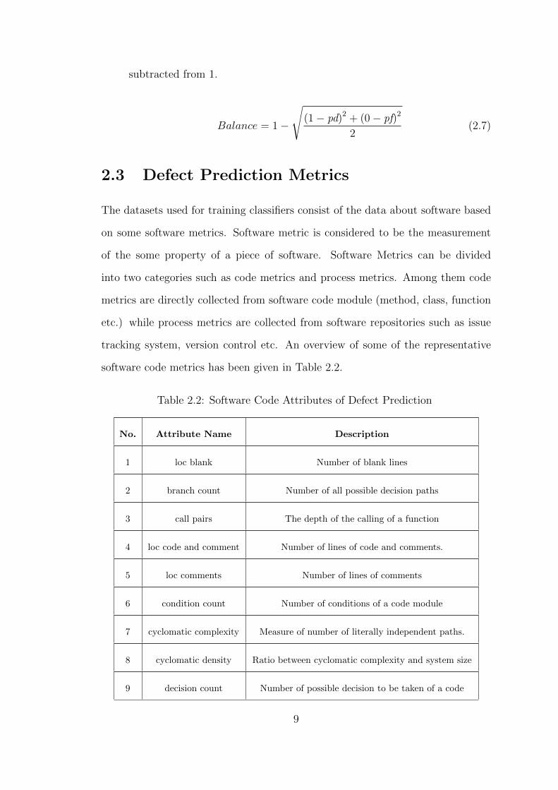
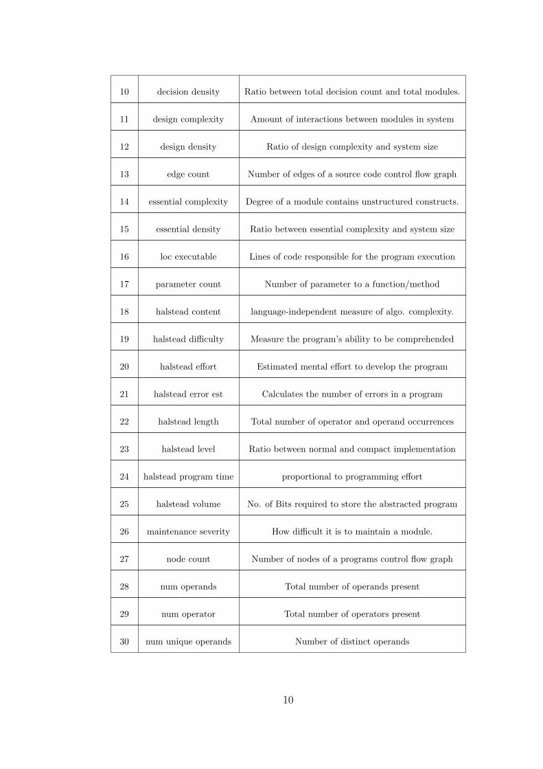
2.3 Defect Prediction Metrics

The datasets used for training classifiers consist of the data about software based

on some software metrics. Software metric is considered to be the measurement

of the some property of a piece of software. Software Metrics can be divided

into two categories such as code metrics and process metrics. Among them code

metrics are directly collected from software code module (method, class, function

etc.) while process metrics are collected from software repositories such as issue

tracking system, version control etc. An overview of some of the representative

software code metrics has been given in Table 2.2.

Table 2.2: Software Code Attributes of Defect Prediction

No. Attribute Name Description

1 loc blank Number of blank lines

2 branch count Number of all possible decision paths

3 call pairs The depth of the calling of a function

4 loc code and comment Number of lines of code and comments.

5 loc comments Number of lines of comments

6 condition count Number of conditions of a code module

7 cyclomatic complexity Measure of number of literally independent paths.

8 cyclomatic density Ratio between cyclomatic complexity and system size

9 decision count Number of possible decision to be taken of a code

9

10 decision density Ratio between total decision count and total modules.

11 design complexity Amount of interactions between modules in system

12 design density Ratio of design complexity and system size

13 edge count Number of edges of a source code control flow graph

14 essential complexity Degree of a module contains unstructured constructs.

15 essential density Ratio between essential complexity and system size

16 loc executable Lines of code responsible for the program execution

17 parameter count Number of parameter to a function/method

18 halstead content language-independent measure of algo. complexity.

19 halstead difficulty Measure the program’s ability to be comprehended

20 halstead effort Estimated mental effort to develop the program

21 halstead error est Calculates the number of errors in a program

22 halstead length Total number of operator and operand occurrences

23 halstead level Ratio between normal and compact implementation

24 halstead program time proportional to programming effort

25 halstead volume No. of Bits required to store the abstracted program

26 maintenance severity How difficult it is to maintain a module.

27 node count Number of nodes of a programs control flow graph

28 num operands Total number of operands present

29 num operator Total number of operators present

30 num unique operands Number of distinct operands

10

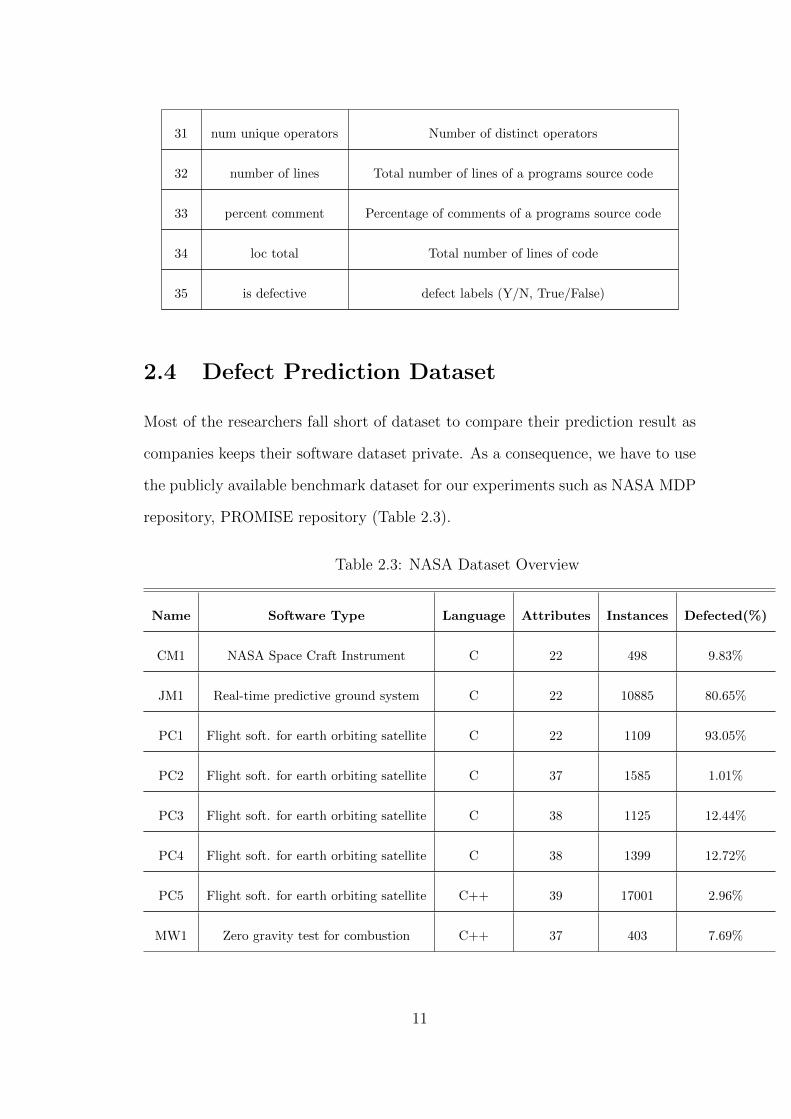
31 num unique operators Number of distinct operators

32 number of lines Total number of lines of a programs source code

33 percent comment Percentage of comments of a programs source code

34 loc total Total number of lines of code

35 is defective defect labels (Y/N, True/False)

2.4 Defect Prediction Dataset

Most of the researchers fall short of dataset to compare their prediction result as

companies keeps their software dataset private. As a consequence, we have to use

the publicly available benchmark dataset for our experiments such as NASA MDP

repository, PROMISE repository (Table 2.3).

Table 2.3: NASA Dataset Overview

Name Software Type Language Attributes Instances Defected(%)

CM1 NASA Space Craft Instrument C 22 498 9.83%

JM1 Real-time predictive ground system C 22 10885 80.65%

PC1 Flight soft. for earth orbiting satellite C 22 1109 93.05%

PC2 Flight soft. for earth orbiting satellite C 37 1585 1.01%

PC3 Flight soft. for earth orbiting satellite C 38 1125 12.44%

PC4 Flight soft. for earth orbiting satellite C 38 1399 12.72%

PC5 Flight soft. for earth orbiting satellite C++ 39 17001 2.96%

MW1 Zero gravity test for combustion C++ 37 403 7.69%

11

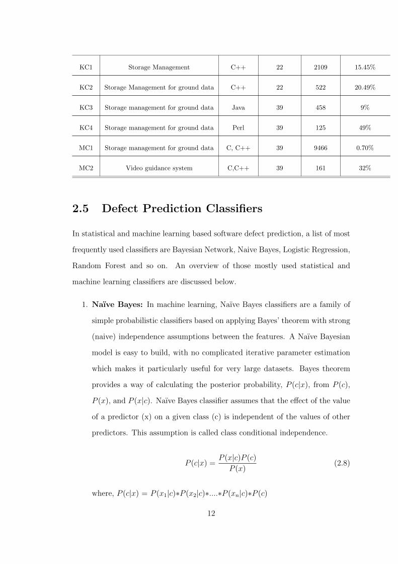
KC1 Storage Management C++ 22 2109 15.45%

KC2 Storage Management for ground data C++ 22 522 20.49%

KC3 Storage management for ground data Java 39 458 9%

KC4 Storage management for ground data Perl 39 125 49%

MC1 Storage management for ground data C, C++ 39 9466 0.70%

MC2 Video guidance system C,C++ 39 161 32%

2.5 Defect Prediction Classifiers

In statistical and machine learning based software defect prediction, a list of most

frequently used classifiers are Bayesian Network, Naive Bayes, Logistic Regression,

Random Forest and so on. An overview of those mostly used statistical and

machine learning classifiers are discussed below.

1. Naıve Bayes: In machine learning, Naıve Bayes classifiers are a family of

simple probabilistic classifiers based on applying Bayes’ theorem with strong

(naive) independence assumptions between the features. A Naıve Bayesian

model is easy to build, with no complicated iterative parameter estimation

which makes it particularly useful for very large datasets. Bayes theorem

provides a way of calculating the posterior probability, P (c|x), from P (c),

P (x), and P (x|c). Naıve Bayes classifier assumes that the effect of the value

of a predictor (x) on a given class (c) is independent of the values of other

predictors. This assumption is called class conditional independence.

P (c|x) =P (x|c)P (c)

P (x)(2.8)

where, P (c|x) = P (x1|c)∗P (x2|c)∗....∗P (xn|c)∗P (c)

12

• P (c|x) is the posterior probability of class (target)given predictor (at-

tribute).

• P (c) is the prior probability of class.

• P (x|c) is the likelihood which is the probability of predictor given class.

• P (x) is the prior probability of predictor.

2. Logistic Regression: Logistic regression is a statistical method for ana-

lyzing a dataset in which there are one or more independent variables that

determine an outcome. The outcome is measured with a dichotomous vari-

able (in which there are only two possible outcomes).In logistic regression,

the dependent variable is binary or dichotomous, i.e. it only contains data

coded as 1 (TRUE, success, pregnant, etc. ) or 0 (FALSE, failure, non-

pregnant, etc.).

The goal of logistic regression is to find the best fitting (yet biologically rea-

sonable) model to describe the relationship between the dichotomous charac-

teristic of interest (dependent variable = response or outcome variable) and

a set of independent (predictor or explanatory) variables. Logistic regression

generates the coefficients (and its standard errors and significance levels) of

a formula to predict a logit transformation of the probability of presence of

the characteristic of interest:

logit(p)= b0 + b1X1 + b2X2 + ...... bkXk

where p is the probability of presence of the characteristic of interest. The

logit transformation is defined as the logged odds:

odds =P

1− P=

probabilityofpresenceofcharacteristic

probabilityofpresenceofcharacteristic(2.9)

and

13

logit(P ) = ln(P

1− P) (2.10)

3. Decision Tree: Decision Trees are excellent classifier choosing between

several courses of action. It provides a highly effective structure within which

we can lay out options and investigate the possible outcomes of choosing

those options. They also help to form a balanced picture of the risks and

rewards associated with each possible course of action.

4. Random Forest: Random forest is a classification method based on en-

semble learning that operate by constructing a multitude of decision trees.

The response of each tree depends on a set of predictor values chosen in-

dependently and with the same distribution for all trees in the forest. For

classification problems, given a set of simple trees and a set of random pre-

dictor variables, the random forest method defines a margin function that

measures the extent to which the average number of votes for the correct

class exceeds the average vote for any other class present in the dependent

variable. This measure provides us not only with a convenient way of making

predictions, but also with a way of associating a confidence measure with

those predictions.

5. Bayesian Network: Bayesian network is a graphical model which encodes

probabilistic relationships among variables of interest. These graphical struc-

ture represents knowledge about an uncertain domain. In the graphical

model, each node represents a random variable and the edges are used to

represent the probabilistic dependencies among those variables. In Bayesian

network graph theory, probability theory, computer science and statistics are

combined which makes this a popular models in the last decade in machine

14

learning, text mining, natural language processing and so on.

2.6 Summary

In this chapter, we discussed the importance as well as the process of software de-

fect prediction. A detail overview of software attributes, datasets used for building

the prediction model are given here. Moreover, we summarized different types of

performance measurement metrics and classifiers along with their utilities.

15

Chapter 3

Literature Review of Software

Defect Prediction

In the recent years, software defect prediction has been become one of the most

important research issues in software engineering due to its great contribution in

improving the quality and productivity of software. In this chapter, the previous

work explored by different researchers in this context has been presented and

analyzed. Based on the existing literature, it is found that researchers emphasis

on different issues for Software Defect prediction including pre-processing of data,

attribute selection and classification methods. Moreover, the defect prediction

process can be categorized into two sections: Within-Project and Cross-Project

defect prediction based on the datasets. In case of insufficient datasets, cross-

project defect prediction has been done where training and test datasets come

from different projects. NASA MDP Repository and PROMISE Date Repository

are the mostly used available datasets in this field.

16

3.1 Pre-processing

The pre-processing strategy is a significant step while using the datasets in the ex-

periment. Sheppard et al. [7] analyzed different versions of NASA defects datasets

and showed the importance of pre-processing due to the presence of various in-

consistencies like missing and conflicting values, features with identical cases etc.

on the datasets. Because this erroneous and implausible value of data can lead to

the prediction result in an incorrect conclusion. Gray et al. [8] also explained the

need of data pre-processing before training the classifier and conducted five stages

of data cleaning process for 13 sets of original NASA dataset. Their concern arises

due to the presence of identical data both in training and testing sets as a result

of data replication. The cleaning method consists of five stages including the dele-

tion of constant and repeated attributes, replacing the missing values, enforcing

integrity of domain specific expertise and removing redundant and inconsistent

instances. The findings of this experiment reveal that the processed datasets be-

come 6-90% less from their original after cleaning and it improves the accuracy of

defect prediction.

Log-filtering, z-score, min-max are some widely used data pre-processing tech-

niques introduced in various researches [7, 9, 10, 11]. Nam et al. [10] used z-score,

variants of z-score and min-max normalization methods in their study in order

to provide all the values an equivalent weight to improve the prediction perfor-

mances. In another study, Gray et al. [11] normalized the data from -1 to +1 for

compressing the range of values. Little changes to data representation can affect

the results of feature selection and defect prediction greatly [11]. Song et al. [12]

utilized log-filtering preprocessor by replacing the numeric values with their log-

arithms, and showed that it performed well with Nave Bays classifier. Moreover,

log filtering can handle the extreme values and its normal distribution better suits

to data [13]. Menzies et al. [6] also processed the datasets using the logarithmic

17

method for improving the prediction performance.

3.2 Attribute Selection

Various attribute selection methods have already been proposed till to date. The

feature selection methods can be divided into two classes based on how they in-

tegrate the selection algorithm and the model building. Filter methods select the

attributes relying on the characteristic of the attributes without having any de-

pendency on the learning algorithm. On the other hand, wrapper based attribute

selection method include the predictor classification algorithm as a part of evalu-

ating the attribute subsets. Both type of selection algorithm have been discussed

here.

An attribute-ranking method was proposed in [2], which focused on select-

ing the minimum number of attributes required for an effective defect prediction

model. To do that, they proposed a threshold-based feature selection method

to come up with the necessary metrics for defect prediction. Five versions of

the proposed selection technique have been experimented creating different size

of metric subsets to assess their effectiveness at the time of defect prediction.

The versions are specified by five performances metrics-Mutual Information (MI),

Kolmogorov-Smirnov (KS), Deviance (DV), Area Under the ROC (Receiver Op-

erating Characteristic) Curve (AUC), and Area Under the Precision-Recall Curve

(PRC).They revealed that only three metrics are enough for SDP. However, it is

not confirmed that it will work with all datasets. Jobaer et al. [14] provided a

technique for choosing the best set of attributes in order to build a good prediction

model. Authors utilized a cardinality to choose the best set of attributes. How-

ever, the selection of this cardinality is heuristically defined which will not work

in general. Further, the frequency based ranking also might fail in many cases.

Gao et al. [4] introduced a hybrid attribute selection approach that first cat-

18

egorizes the important metrics by feature ranking approach and then chooses the

subsets of metrics through features subset selection approach. Another paper [1]

proposed a technique called hybrid attribute selection approach consisting of both

feature ranking and feature subset selection. In this experiment, five feature rank-

ing techniques including chi-square (CS), information gain (IG), gain ratio (GR),

KolmogorovSmirnov statistic (KS), two forms of the Relief algorithm (RLF), and

symmetrical uncertainty (SU) were studied along with four feature subset selection

algorithms: exhaustive search (ES), heuristic search (HS), and automatic hybrid

search (AHS) and no subset selection. The hybrid method first categorizes the

important attributes and reduces the search space using a search algorithm in

feature ranking approach. Then it chooses the subsets of metrics through features

subset selection approaches. It is found that automatic hybrid search (AHS) is

better than other search algorithm in the context of choosing attributes and the

removal of 85% metrics can enhance the performance of the prediction model in

some cases.

A general defect prediction framework consisting of a data pre-processor, at-

tribute selection, and learning algorithms is proposed by et al. [12]. They made

total 12 learning schemes by combining two data pre-processor, two wrapper based

attribute selection (forward selection and backward elimination) and three learn-

ing algorithms ( NB, J48, OneR) to find out the best learning scheme. The best

results are achieved for different datasets with different combinations of these pre-

processing, feature selection and learning algorithms. However, in their proposal,

there is no clear indication about which combination should be used for a partic-

ular dataset.

It is found in the most researches that the performance of cross-project defect

prediction is worse compared to within-project due to the differences of distri-

bution between source and target projects. In this Paper [15], the performance

of cross-project defect prediction has been evaluated from a different perspective

19

called cost-sensitive analysis using 9 Apache Software Foundation projects con-

sisting of 38 releases. Prediction models are built under Logistic Regression and

compared on the basis of AUC, Precision, F-measure and AUCEC (area under the

cost-effectiveness curve) measurement between cross-project and within-project.

The experiment shows that cross-project defeat prediction provides a good perfor-

mance like within-project and better one than random prediction if the resources

are constrained. HE et al. [16] investigates the effectiveness of the different pre-

dictors on a simplified metrics set for both within-project and cross-project defect

prediction. The authors proposed a selection technique including an evaluator

called CfsSubsetEval and a search algorithm named GreedyStepwise. The find-

ings of the experiment shows that the predictors with minimal metrics sets provide

better result and simple classifiers like Nave Bayes perform well in this context.

In order to improve the result of cross-project defect prediction a new novel

transfer learning approach has been proposed by Nam et al. [16] named TCA+

to select the proper normalization options for TCA. The result shows TCA+

outperforms the entire baseline and it is also comparable to within-project defect

prediction.

3.3 Classification

Various machine learning algorithms have been investigated in different ways to

find the best one that performs well in the respective context. Naıve Bayes, deci-

sion tree, logistic regression, neural networks, support vector machine are widely

used classifiers in the field of SDP.

Menzies et al. [6] used J48, OneR and Naıve Bays classifiers in their research

and found that Nave Bays performs better than others. Challagulla [17] analyzed

different classifiers and concluded that IBL (instance based learning) and 1R (1-

Rule) were in a better condition in respect of accuracy of finding bugs properly.

20

In [18], the authors investigated the statistical comparison of 22 classifiers in the

respect of AUC performance which indicated that the accuracy of these classifiers

of top 17 does not differ much unlike previous researches.

Besides, Five class imbalance learning methods that are Random undersam-

pling (RUS), the balanced version of random undersampling (RUS-bal), threshold-

moving (THM), AdaBoost.NC (BNC) and SMOTEBoost (SMB) have been stud-

ied in this paper [19] using two top-ranked classifiers Naıve Bayes and Random

Forest for the purpose of improving the performances of defect prediction. Ad-

aBoost.NC shows the best result in terms of balance, G-mean, and AU.

3.4 Summary

Different research works on software defect prediction have been gathered in this

chapter with a view to reviewing their methodology and results. We discussed

the previous researches into three categories: Pre-processing, Attribute Selection,

Classification. Though many attribute selection process have been proposed till

now, there exists some limitations of these works. Therefore, It leads us to propose

a new method which can produce better result in predicting the defects.

21

Chapter 4

Proposed Methodology

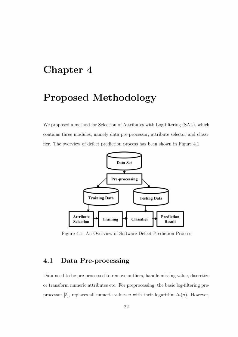
We proposed a method for Selection of Attributes with Log-filtering (SAL), which

contains three modules, namely data pre-processor, attribute selector and classi-

fier. The overview of defect prediction process has been shown in Figure 4.1

Figure 4.1: An Overview of Software Defect Prediction Process

4.1 Data Pre-processing

Data need to be pre-processed to remove outliers, handle missing value, discretize

or transform numeric attributes etc. For preprocessing, the basic log-filtering pre-

processor [5], replaces all numeric values n with their logarithm ln(n). However,

22

we use ln(n+∈) instead of ln(n), where ∈ is a small value and is set based on

rigorous experiment (Figure 5.1).

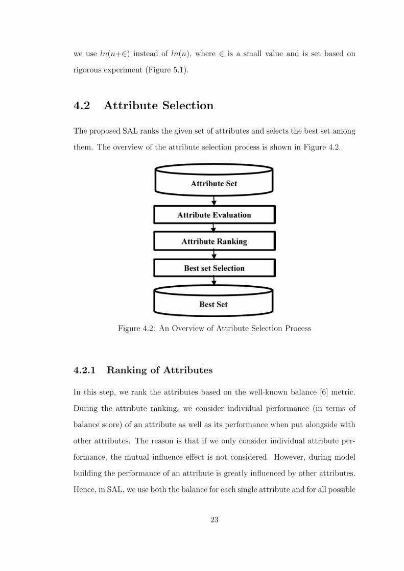
4.2 Attribute Selection

The proposed SAL ranks the given set of attributes and selects the best set among

them. The overview of the attribute selection process is shown in Figure 4.2.

Figure 4.2: An Overview of Attribute Selection Process

4.2.1 Ranking of Attributes

In this step, we rank the attributes based on the well-known balance [6] metric.

During the attribute ranking, we consider individual performance (in terms of

balance score) of an attribute as well as its performance when put alongside with

other attributes. The reason is that if we only consider individual attribute per-

formance, the mutual influence effect is not considered. However, during model

building the performance of an attribute is greatly influenced by other attributes.

Hence, in SAL, we use both the balance for each single attribute and for all possible

23

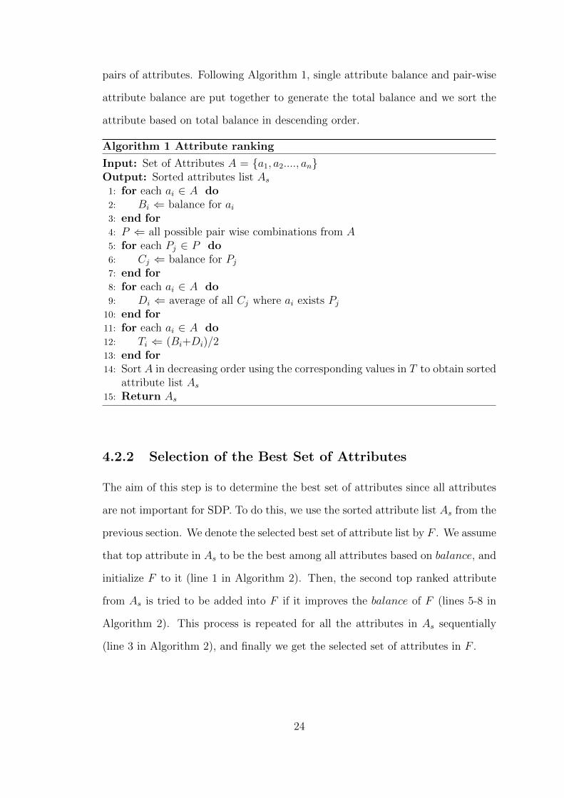
pairs of attributes. Following Algorithm 1, single attribute balance and pair-wise

attribute balance are put together to generate the total balance and we sort the

attribute based on total balance in descending order.

Algorithm 1 Attribute ranking

Input: Set of Attributes A = {a1, a2...., an}Output: Sorted attributes list As

1: for each ai ∈ A do2: Bi ⇐ balance for ai3: end for4: P ⇐ all possible pair wise combinations from A5: for each Pj ∈ P do6: Cj ⇐ balance for Pj

7: end for8: for each ai ∈ A do9: Di ⇐ average of all Cj where ai exists Pj

10: end for11: for each ai ∈ A do12: Ti ⇐ (Bi+Di)/213: end for14: Sort A in decreasing order using the corresponding values in T to obtain sorted

attribute list As

15: Return As

4.2.2 Selection of the Best Set of Attributes

The aim of this step is to determine the best set of attributes since all attributes

are not important for SDP. To do this, we use the sorted attribute list As from the

previous section. We denote the selected best set of attribute list by F . We assume

that top attribute in As to be the best among all attributes based on balance, and

initialize F to it (line 1 in Algorithm 2). Then, the second top ranked attribute

from As is tried to be added into F if it improves the balance of F (lines 5-8 in

Algorithm 2). This process is repeated for all the attributes in As sequentially

(line 3 in Algorithm 2), and finally we get the selected set of attributes in F .

24

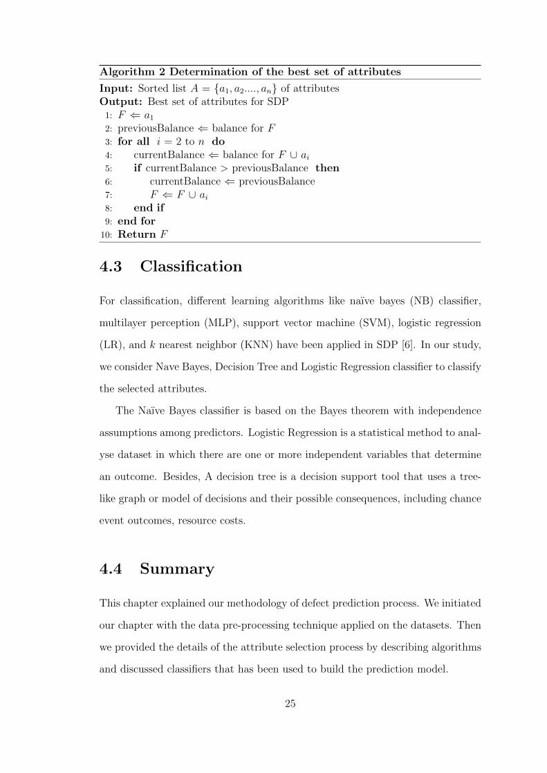
Algorithm 2 Determination of the best set of attributes

Input: Sorted list A = {a1, a2...., an} of attributesOutput: Best set of attributes for SDP

1: F ⇐ a12: previousBalance ⇐ balance for F3: for all i = 2 to n do4: currentBalance ⇐ balance for F ∪ ai5: if currentBalance > previousBalance then6: currentBalance ⇐ previousBalance7: F ⇐ F ∪ ai8: end if9: end for

10: Return F

4.3 Classification

For classification, different learning algorithms like naıve bayes (NB) classifier,

multilayer perception (MLP), support vector machine (SVM), logistic regression

(LR), and k nearest neighbor (KNN) have been applied in SDP [6]. In our study,

we consider Nave Bayes, Decision Tree and Logistic Regression classifier to classify

the selected attributes.

The Naıve Bayes classifier is based on the Bayes theorem with independence

assumptions among predictors. Logistic Regression is a statistical method to anal-

yse dataset in which there are one or more independent variables that determine

an outcome. Besides, A decision tree is a decision support tool that uses a tree-

like graph or model of decisions and their possible consequences, including chance

event outcomes, resource costs.

4.4 Summary

This chapter explained our methodology of defect prediction process. We initiated

our chapter with the data pre-processing technique applied on the datasets. Then

we provided the details of the attribute selection process by describing algorithms

and discussed classifiers that has been used to build the prediction model.

25

Chapter 5

Experimental Results and

Discussion

In this section, we present the experimental evaluation of the proposed SAL in

comparison with other currently available methods for SDP. We first describe the

simulation setup including evaluation metrics and then present the experimental

results.

5.1 Evaluation Metrics

We have used Balance and AUC to measure the perfromance of prediction re-

sult.The equation for computing the balance according to [12, 6] is shown below

using (5.1).

balance = 1−√

(1− pd)2 + (0− pf)2√2

(5.1)

Another evaluation is the Receiver Operating Characteristic (ROC) curve

which provides a graphical visualization of the results. The Area Under the ROC

Curve (AUC) also provides a quality measure for classification problem [20].

26

5.2 Implementation Details

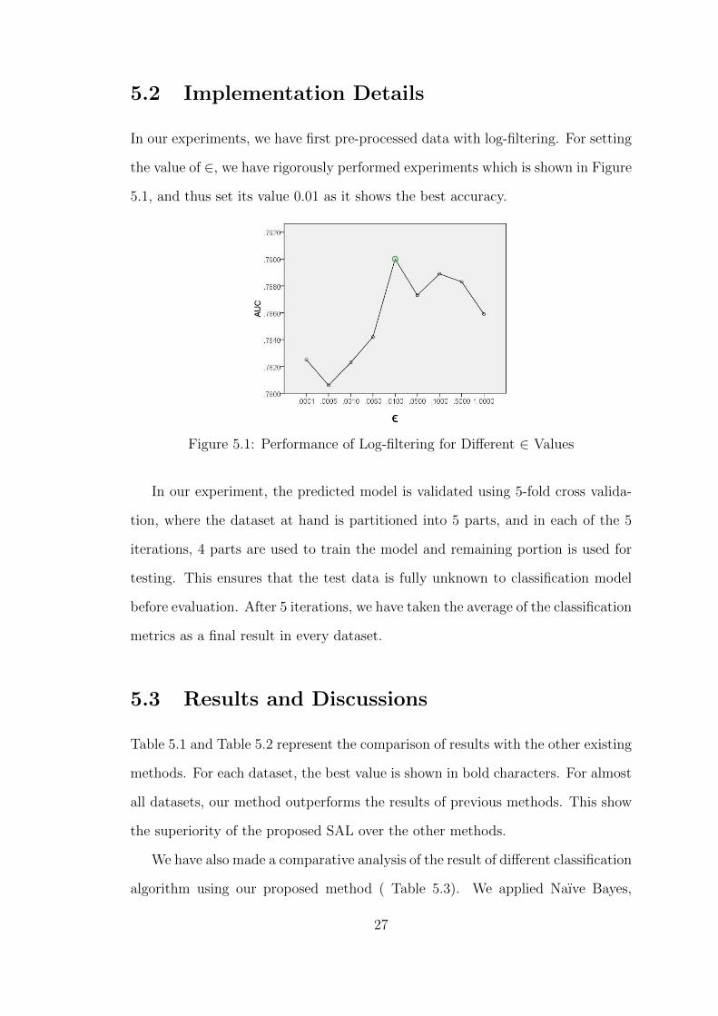
In our experiments, we have first pre-processed data with log-filtering. For setting

the value of ∈, we have rigorously performed experiments which is shown in Figure

5.1, and thus set its value 0.01 as it shows the best accuracy.

Figure 5.1: Performance of Log-filtering for Different ∈ Values

In our experiment, the predicted model is validated using 5-fold cross valida-

tion, where the dataset at hand is partitioned into 5 parts, and in each of the 5

iterations, 4 parts are used to train the model and remaining portion is used for

testing. This ensures that the test data is fully unknown to classification model

before evaluation. After 5 iterations, we have taken the average of the classification

metrics as a final result in every dataset.

5.3 Results and Discussions

Table 5.1 and Table 5.2 represent the comparison of results with the other existing

methods. For each dataset, the best value is shown in bold characters. For almost

all datasets, our method outperforms the results of previous methods. This show

the superiority of the proposed SAL over the other methods.

We have also made a comparative analysis of the result of different classification

algorithm using our proposed method ( Table 5.3). We applied Naıve Bayes,

27

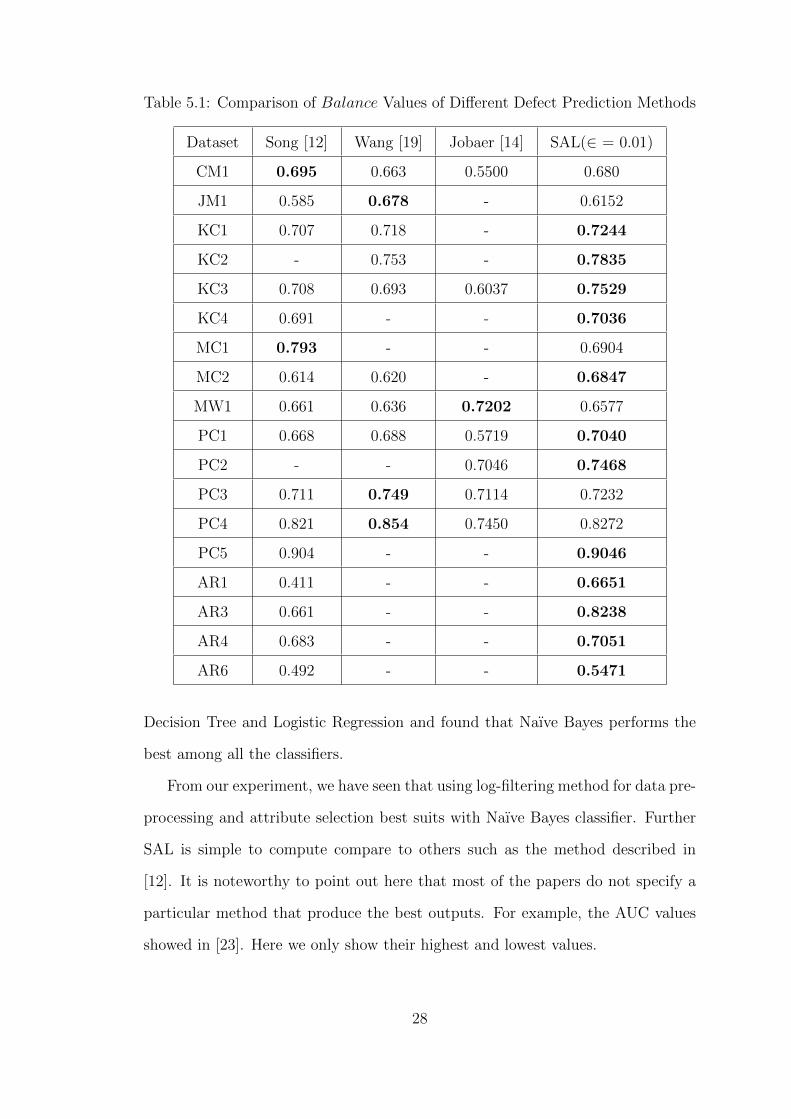
Table 5.1: Comparison of Balance Values of Different Defect Prediction Methods

Dataset Song [12] Wang [19] Jobaer [14] SAL(∈ = 0.01)

CM1 0.695 0.663 0.5500 0.680

JM1 0.585 0.678 - 0.6152

KC1 0.707 0.718 - 0.7244

KC2 - 0.753 - 0.7835

KC3 0.708 0.693 0.6037 0.7529

KC4 0.691 - - 0.7036

MC1 0.793 - - 0.6904

MC2 0.614 0.620 - 0.6847

MW1 0.661 0.636 0.7202 0.6577

PC1 0.668 0.688 0.5719 0.7040

PC2 - - 0.7046 0.7468

PC3 0.711 0.749 0.7114 0.7232

PC4 0.821 0.854 0.7450 0.8272

PC5 0.904 - - 0.9046

AR1 0.411 - - 0.6651

AR3 0.661 - - 0.8238

AR4 0.683 - - 0.7051

AR6 0.492 - - 0.5471

Decision Tree and Logistic Regression and found that Naıve Bayes performs the

best among all the classifiers.

From our experiment, we have seen that using log-filtering method for data pre-

processing and attribute selection best suits with Naıve Bayes classifier. Further

SAL is simple to compute compare to others such as the method described in

[12]. It is noteworthy to point out here that most of the papers do not specify a

particular method that produce the best outputs. For example, the AUC values

showed in [23]. Here we only show their highest and lowest values.

28

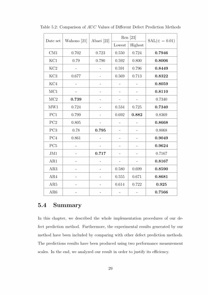
Table 5.2: Comparison of AUC Values of Different Defect Prediction Methods

Date set Wahono [21] Abaei [22]Ren [23]

SAL(∈ = 0.01)Lowest Highest

CM1 0.702 0.723 0.550 0.724 0.7946

KC1 0.79 0.790 0.592 0.800 0.8006

KC2 - - 0.591 0.796 0.8449

KC3 0.677 - 0.569 0.713 0.8322

KC4 - - - - 0.8059

MC1 - - - - 0.8110

MC2 0.739 - - - 0.7340

MW1 0.724 - 0.534 0.725 0.7340

PC1 0.799 - 0.692 0.882 0.8369

PC2 0.805 - - - 0.8668

PC3 0.78 0.795 - - 0.8068

PC4 0.861 - - - 0.9049

PC5 - - - - 0.9624

JM1 - 0.717 - - 0.7167

AR1 - - - - 0.8167

AR3 - - 0.580 0.699 0.8590

AR4 - - 0.555 0.671 0.8681

AR5 - - 0.614 0.722 0.925

AR6 - - - - 0.7566

5.4 Summary

In this chapter, we described the whole implementation procedures of our de-

fect prediction method. Furthermore, the experimental results generated by our

method have been included by comparing with other defect prediction methods.

The predictions results have been produced using two performance measurement

scales. In the end, we analyzed our result in order to justify its efficiency.

29

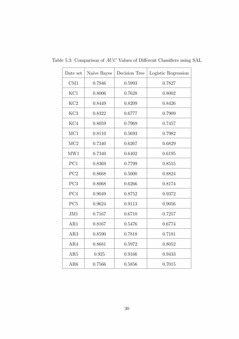
Table 5.3: Comparison of AUC Values of Different Classifiers using SAL

Date set Naıve Bayes Decision Tree Logistic Regression

CM1 0.7946 0.5993 0.7827

KC1 0.8006 0.7628 0.8002

KC2 0.8449 0.8209 0.8426

KC3 0.8322 0.6777 0.7909

KC4 0.8059 0.7969 0.7457

MC1 0.8110 0.5693 0.7982

MC2 0.7340 0.6267 0.6829

MW1 0.7340 0.6402 0.6195

PC1 0.8369 0.7799 0.8555

PC2 0.8668 0.5000 0.8824

PC3 0.8068 0.6266 0.8174

PC4 0.9049 0.8752 0.9372

PC5 0.9624 0.9113 0.9056

JM1 0.7167 0.6710 0.7257

AR1 0.8167 0.5476 0.6774

AR3 0.8590 0.7818 0.7181

AR4 0.8681 0.5972 0.8052

AR5 0.925 0.9166 0.9433

AR6 0.7566 0.5856 0.7015

30

Chapter 6

Conclusion

At present defect prediction has become one of the most important research topics

in the field of software engineering. For improving the prediction result, we need

to find the standard sets of attributes which is a very challenging task. There-

fore,exploring the best sets of attributes for training the classifiers has become one

of the key issues in SDP.

In our thesis, we have proposed an attribute selection method which includes

ranking of attributes and then selecting the best set. Our ranking technique is

built based on the balances of different combinations of attributes.From this or-

dered attributes, we finally determine our best group of attributes.We compared

the performance of our technique using Balance and AUC measurement scales.

For classification, we have used Nave Bayes, Decision Tree and Logistic Regres-

sion algorithm to train our datasets. In our proposed method we considered the

influence of one attribute over another one using their combinations as the at-

tributes have dependency among them. The influence of paired attributes while

ranking them has not taken into concern in other existing methods. However, we

only calculated the value of pair-wise combinations instead of all combinations to

avoid the complexity.According to the results of experiment, our proposed SAL

provides better accuracy of prediction.

31

Our thesis work considered only eighteen datasets for defect prediction. In

future, we will expand our work using other publicly available datasets for ex-

periment which will strengthen the efficiency of our method. Apart from nave

bayes, we want to study the performances of other classifiers to improve our re-

sult. Moreover, we have a plan to apply our proposed method for cross-project

defect prediction.

32

Bibliography

[1] K. Gao, T. M. Khoshgoftaar, H. Wang, and N. Seliya, “Choosing softwaremetrics for defect prediction: an investigation on feature selection tech-niques,” Software: Practice and Experience, vol. 41, no. 5, pp. 579–606, 2011.

[2] H. Wang, T. M. Khoshgoftaar, and N. Seliya, “How many software metricsshould be selected for defect prediction?,” in FLAIRS Conference, 2011.

[3] H. Wang, T. M. Khoshgoftaar, and J. Van Hulse, “A comparative study ofthreshold-based feature selection techniques,” in Granular Computing (GrC),2010 IEEE International Conference on, pp. 499–504, IEEE, 2010.

[4] K. Gao, T. M. Khoshgoftaar, and H. Wang, “An empirical investigation offilter attribute selection techniques for software quality classification,” in In-formation Reuse & Integration, 2009. IRI’09. IEEE International Conferenceon, pp. 272–277, IEEE, 2009.

[5] K. O. Elish and M. O. Elish, “Predicting defect-prone software modules usingsupport vector machines,” Journal of Systems and Software, vol. 81, no. 5,pp. 649–660, 2008.

[6] T. Menzies, J. Greenwald, and A. Frank, “Data mining static code attributesto learn defect predictors,” Software Engineering, IEEE Transactions on,vol. 33, no. 1, pp. 2–13, 2007.

[7] M. Shepperd, Q. Song, Z. Sun, and C. Mair, “Data quality: Some commentson the nasa software defect datasets,” Software Engineering, IEEE Transac-tions on, vol. 39, no. 9, pp. 1208–1215, 2013.

[8] D. Gray, D. Bowes, N. Davey, Y. Sun, and B. Christianson, “The misuse ofthe nasa metrics data program data sets for automated software defect pre-diction,” in Evaluation & Assessment in Software Engineering (EASE 2011),15th Annual Conference on, pp. 96–103, IET, 2011.

[9] J. Yang and V. Honavar, “Feature subset selection using a genetic algorithm,”in Feature extraction, construction and selection, pp. 117–136, Springer, 1998.

[10] J. Nam, S. J. Pan, and S. Kim, “Transfer defect learning,” in Proceedingsof the 2013 International Conference on Software Engineering, pp. 382–391,IEEE Press, 2013.

33

[11] D. Gray, D. Bowes, N. Davey, Y. Sun, and B. Christianson, “Using the sup-port vector machine as a classification method for software defect predictionwith static code metrics,” in Engineering Applications of Neural Networks,pp. 223–234, Springer, 2009.

[12] Q. Song, Z. Jia, M. Shepperd, S. Ying, and S. Y. J. Liu, “A general soft-ware defect-proneness prediction framework,” Software Engineering, IEEETransactions on, vol. 37, no. 3, pp. 356–370, 2011.

[13] B. Turhan and A. Bener, “A multivariate analysis of static code attributes fordefect prediction,” in Quality Software, 2007. QSIC’07. Seventh InternationalConference on, pp. 231–237, IEEE, 2007.

[14] J. Khan, A. U. Gias, M. S. Siddik, M. H. Rahman, S. M. Khaled, M. Shoyaib,et al., “An attribute selection process for software defect prediction,” in In-formatics, Electronics & Vision (ICIEV), 2014 International Conference on,pp. 1–4, IEEE, 2014.

[15] F. Rahman, D. Posnett, and P. Devanbu, “Recalling the imprecision of cross-project defect prediction,” in Proceedings of the ACM SIGSOFT 20th In-ternational Symposium on the Foundations of Software Engineering, p. 61,ACM, 2012.

[16] P. He, B. Li, X. Liu, J. Chen, and Y. Ma, “An empirical study on softwaredefect prediction with a simplified metric set,” Information and SoftwareTechnology, vol. 59, pp. 170–190, 2015.

[17] V. U. B. Challagulla, F. B. Bastani, I.-L. Yen, and R. A. Paul, “Empiricalassessment of machine learning based software defect prediction techniques,”International Journal on Artificial Intelligence Tools, vol. 17, no. 02, pp. 389–400, 2008.

[18] S. Lessmann, B. Baesens, C. Mues, and S. Pietsch, “Benchmarking classi-fication models for software defect prediction: A proposed framework andnovel findings,” Software Engineering, IEEE Transactions on, vol. 34, no. 4,pp. 485–496, 2008.

[19] S. Wang and X. Yao, “Using class imbalance learning for software defectprediction,” Reliability, IEEE Transactions on, vol. 62, no. 2, pp. 434–443,2013.

[20] T. Fawcett, “An introduction to roc analysis,” Pattern recognition letters,vol. 27, no. 8, pp. 861–874, 2006.

[21] R. S. Wahono and N. S. Herman, “Genetic feature selection for software defectprediction,” Advanced Science Letters, vol. 20, no. 1, pp. 239–244, 2014.

[22] G. Abaei and A. Selamat, “A survey on software fault detection based on dif-ferent prediction approaches,” Vietnam Journal of Computer Science, vol. 1,no. 2, pp. 79–95, 2014.

34

[23] J. Ren, K. Qin, Y. Ma, and G. Luo, “On software defect prediction usingmachine learning,” Journal of Applied Mathematics, vol. 2014, 2014.

35