Machine Learning meets DevOps

MachineLearningmeetsDevOps:whenuncertaintycanbehelpful

Pooyan JamshidiImperial College [email protected]

Software Performance Engineering in the DevOps World, Sept 2016

Motivation

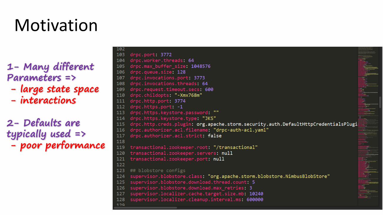
1- Many different Parameters => - large state space- interactions

2- Defaults are typically used =>- poor performance

Motivation

0 1 2 3 4 5average read latency (µs)

×104

0

20

40

60

80

100

120

140

160

obse

rvatio

ns

1000 1200 1400 1600 1800 2000average read latency (µs)

0

10

20

30

40

50

60

70

obse

rvatio

ns

1

1200

1300

1400

1500

1600

1700

1800

1900

1

0.5 1

1.5 2

2.5 3

3.5 4

×10

4(a) cass-20 (b) cass-10

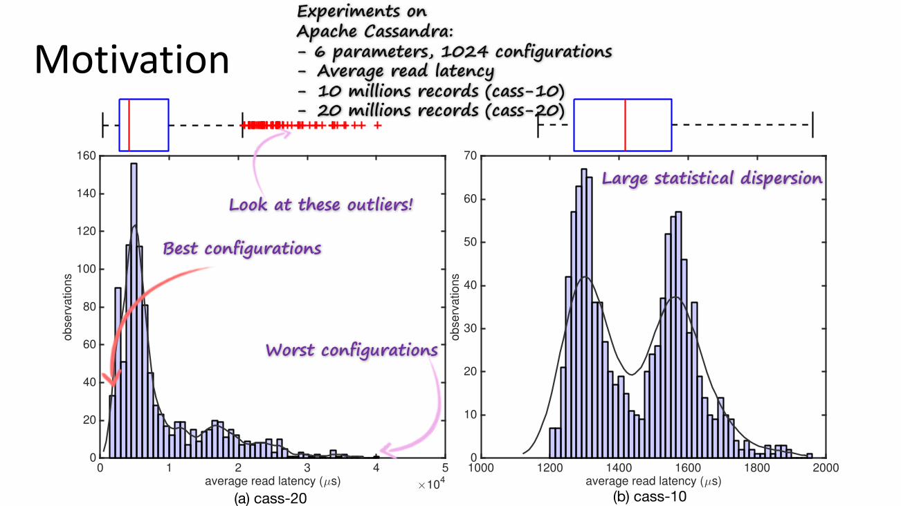
Best configurations

Worst configurations

Experiments on Apache Cassandra:- 6 parameters, 1024 configurations- Average read latency- 10 millions records (cass-10)- 20 millions records (cass-20)

Look at these outliers!Large statistical dispersion

Motivation

0 1000 2000 3000 4000 5000average write latency ( s)

0

50

100

150

200

250

300

350

400

450

500

ob

serv

atio

ns

1

500

1000

1500

2000

2500

3000

3500

4000

4500

5000

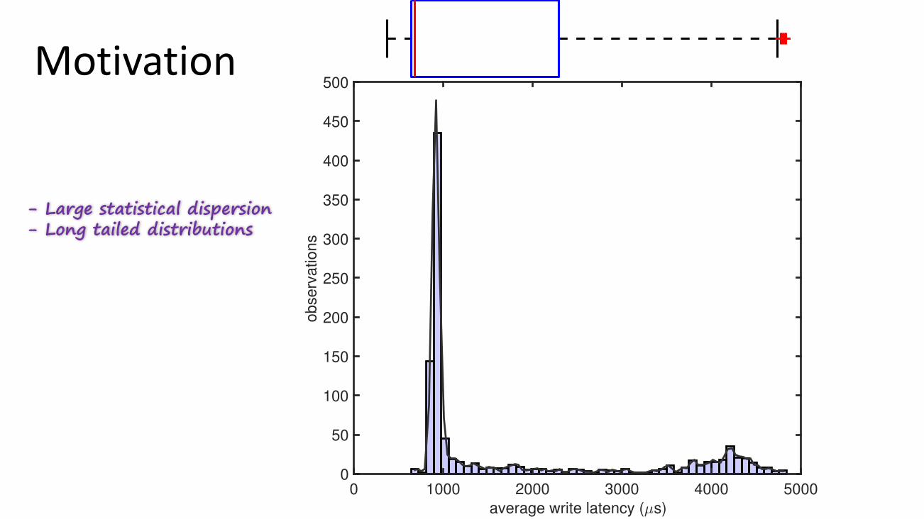
- Large statistical dispersion- Long tailed distributions

Motivation(throughput)

-500 0 500 1000 1500throughput (ops/sec)

0

10

20

30

40

50

60

obse

rvatio

ns

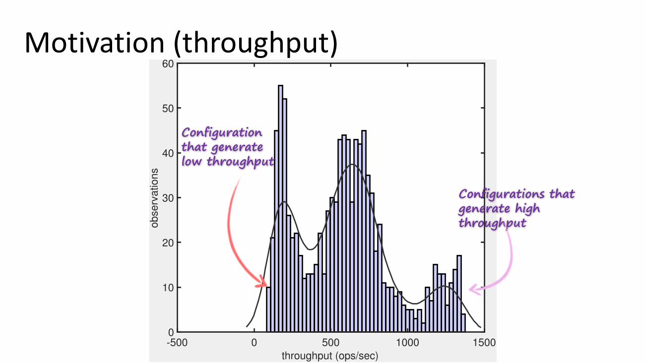
Configuration that generate low throughput

Configurations that generate high throughput

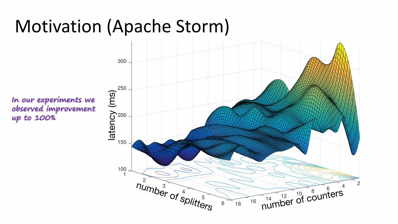
Motivation(ApacheStorm)

number of countersnumber of splitters

late

ncy

(ms)

100

150

1

200

250

2

300

Cubic Interpolation Over Finer Grid

243

684 10

125 14166 18

In our experiments we observed improvement up to 100%

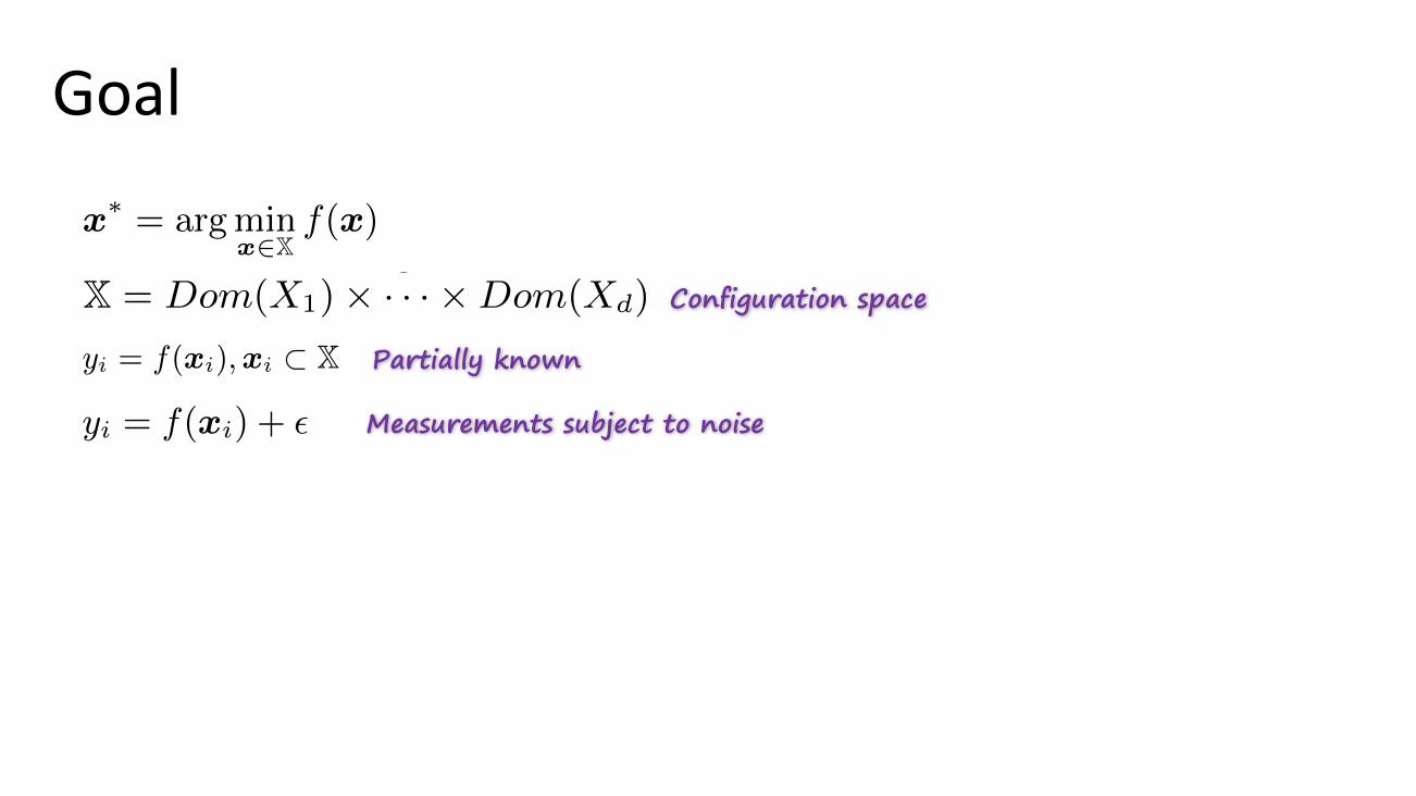
Goal

information from the previous versions, the acquired data onthe current version, and apply a variety of kernel estimators[27] to locate regions where optimal configurations may lie.The key benefit of MTGPs over GPs is that the similaritybetween the response data helps the model to converge tomore accurate predictions much earlier. We experimentallyshow that TL4CO outperforms state-of-the-art configurationtuning methods. Our real configuration datasets are collectedfor three stream processing systems (SPS), implemented withApache Storm, a NoSQL benchmark system with ApacheCassandra, and using a dataset on 6 cloud-based clustersobtained in [21] worth 3 months of experimental time.The rest of this paper is organized as follows. Section 2

overviews the problem and motivates the work via an exam-ple. TL4CO is introduced in Section 3 and then validated inSection 4. Section 5 provides behind the scene and Section 6concludes the paper.

2. PROBLEM AND MOTIVATION

2.1 Problem statementIn this paper, we focus on the problem of optimal system

configuration defined as follows. Let Xi indicate the i-thconfiguration parameter, which ranges in a finite domainDom(Xi). In general, Xi may either indicate (i) integer vari-able such as level of parallelism or (ii) categorical variablesuch as messaging frameworks or Boolean variable such asenabling timeout. We use the terms parameter and factor in-terchangeably; also, with the term option we refer to possiblevalues that can be assigned to a parameter.

We assume that each configuration x 2 X in the configura-tion space X = Dom(X1)⇥ · · ·⇥Dom(Xd) is valid, i.e., thesystem accepts this configuration and the corresponding testresults in a stable performance behavior. The response withconfiguration x is denoted by f(x). Throughout, we assumethat f(·) is latency, however, other metrics for response maybe used. We here consider the problem of finding an optimalconfiguration x

⇤ that globally minimizes f(·) over X:

x

⇤ = argminx2X

f(x) (1)

In fact, the response function f(·) is usually unknown orpartially known, i.e., yi = f(xi),xi ⇢ X. In practice, suchmeasurements may contain noise, i.e., yi = f(xi) + ✏. Thedetermination of the optimal configuration is thus a black-box optimization program subject to noise [27, 33], whichis considerably harder than deterministic optimization. Apopular solution is based on sampling that starts with anumber of sampled configurations. The performance of theexperiments associated to this initial samples can delivera better understanding of f(·) and guide the generation ofthe next round of samples. If properly guided, the processof sample generation-evaluation-feedback-regeneration willeventually converge and the optimal configuration will belocated. However, a sampling-based approach of this kind canbe prohibitively expensive in terms of time or cost (e.g., rentalof cloud resources) considering that a function evaluation inthis case would be costly and the optimization process mayrequire several hundreds of samples to converge.

2.2 Related workSeveral approaches have attempted to address the above

problem. Recursive Random Sampling (RRS) [43] integratesa restarting mechanism into the random sampling to achievehigh search e�ciency. Smart Hill Climbing (SHC) [42] inte-grates the importance sampling with Latin Hypercube Design

(lhd). SHC estimates the local regression at each potentialregion, then it searches toward the steepest descent direction.An approach based on direct search [45] forms a simplexin the parameter space by a number of samples, and itera-tively updates a simplex through a number of well-definedoperations including reflection, expansion, and contractionto guide the sample generation. Quick Optimization viaGuessing (QOG) in [31] speeds up the optimization processexploiting some heuristics to filter out sub-optimal configu-rations. The statistical approach in [33] approximates thejoint distribution of parameters with a Gaussian in order toguide sample generation towards the distribution peak. Amodel-based approach [35] iteratively constructs a regressionmodel representing performance influences. Some approacheslike [8] enable dynamic detection of optimal configurationin dynamic environments. Finally, our earlier work BO4CO[21] uses Bayesian Optimization based on GPs to acceleratethe search process, more details are given later in Section 3.

2.3 SolutionAll the previous e↵orts attempt to improve the sampling

process by exploiting the information that has been gained inthe current task. We define a task as individual tuning cyclethat optimizes a given version of the system under test. As aresult, the learning is limited to the current observations andit still requires hundreds of sample evaluations. In this pa-per, we propose to adopt a transfer learning method to dealwith the search e�ciency in configuration tuning. Ratherthan starting the search from scratch, the approach transfersthe learned knowledge coming from similar versions of thesoftware to accelerate the sampling process in the currentversion. This idea is inspired from several observations arisein real software engineering practice [2, 3]. For instance, (i)in DevOps di↵erent versions of a system is delivered con-tinuously, (ii) Big Data systems are developed using similarframeworks (e.g., Apache Hadoop, Spark, Kafka) and runon similar platforms (e.g., cloud clusters), (iii) and di↵erentversions of a system often share a similar business logic.

To the best of our knowledge, only one study [9] exploresthe possibility of transfer learning in system configuration.The authors learn a Bayesian network in the tuning processof a system and reuse this model for tuning other similarsystems. However, the learning is limited to the structure ofthe Bayesian network. In this paper, we introduce a methodthat not only reuse a model that has been learned previouslybut also the valuable raw data. Therefore, we are not limitedto the accuracy of the learned model. Moreover, we do notconsider Bayesian networks and instead focus on MTGPs.

2.4 MotivationA motivating example. We now illustrate the previous

points on an example. WordCount (cf. Figure 1) is a popularbenchmark [12]. WordCount features a three-layer architec-ture that counts the number of words in the incoming stream.A Processing Element (PE) of type Spout reads the inputmessages from a data source and pushes them to the system.A PE of type Bolt named Splitter is responsible for splittingsentences, which are then counted by the Counter.

Kafka Spout Splitter Bolt Counter Bolt

(sentence) (word)[paintings, 3][poems, 60][letter, 75]

Kafka Topic

Stream to Kafka

File(sentence)

(sentence)

(sen

tenc

e)

Figure 1: WordCount architecture.

2








x

⇤ = argminx2X

f(x) (1)












Kafka Topic

Stream to Kafka

File(sentence)

(sentence)

(sen

tenc

e)


2








x

⇤ = argminx2X

f(x) (1)












Kafka Topic

Stream to Kafka

File(sentence)

(sentence)

(sen

tenc

e)


2








x

⇤ = argminx2X

f(x) (1)












Kafka Topic

Stream to Kafka

File(sentence)

(sentence)

(sen

tenc

e)


2

Partially known

Measurements subject to noise

Configuration space

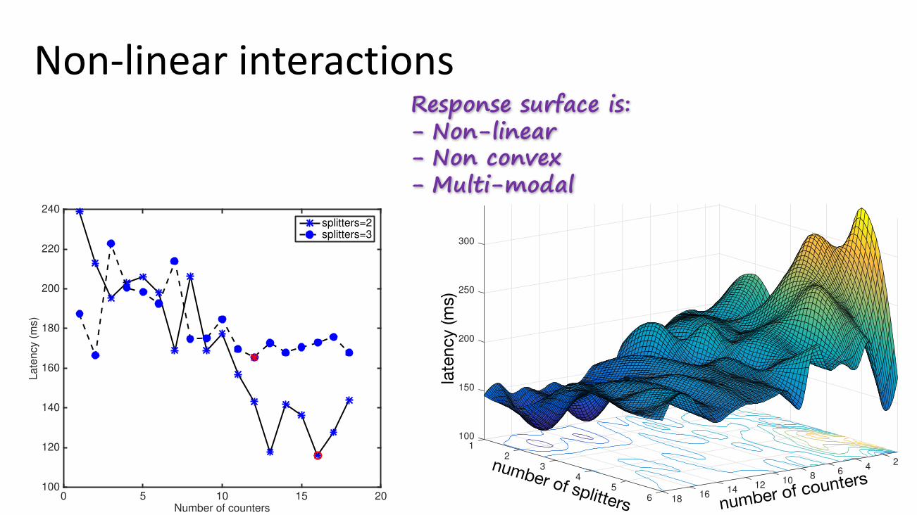
Non-linearinteractions

0 5 10 15 20Number of counters

100

120

140

160

180

200

220

240

Late

ncy

(m

s)

splitters=2splitters=3


late

ncy

(ms)

100

150

1

200

250

2

300


243

684 10

125 14166 18

Response surface is:- Non-linear- Non convex- Multi-modal

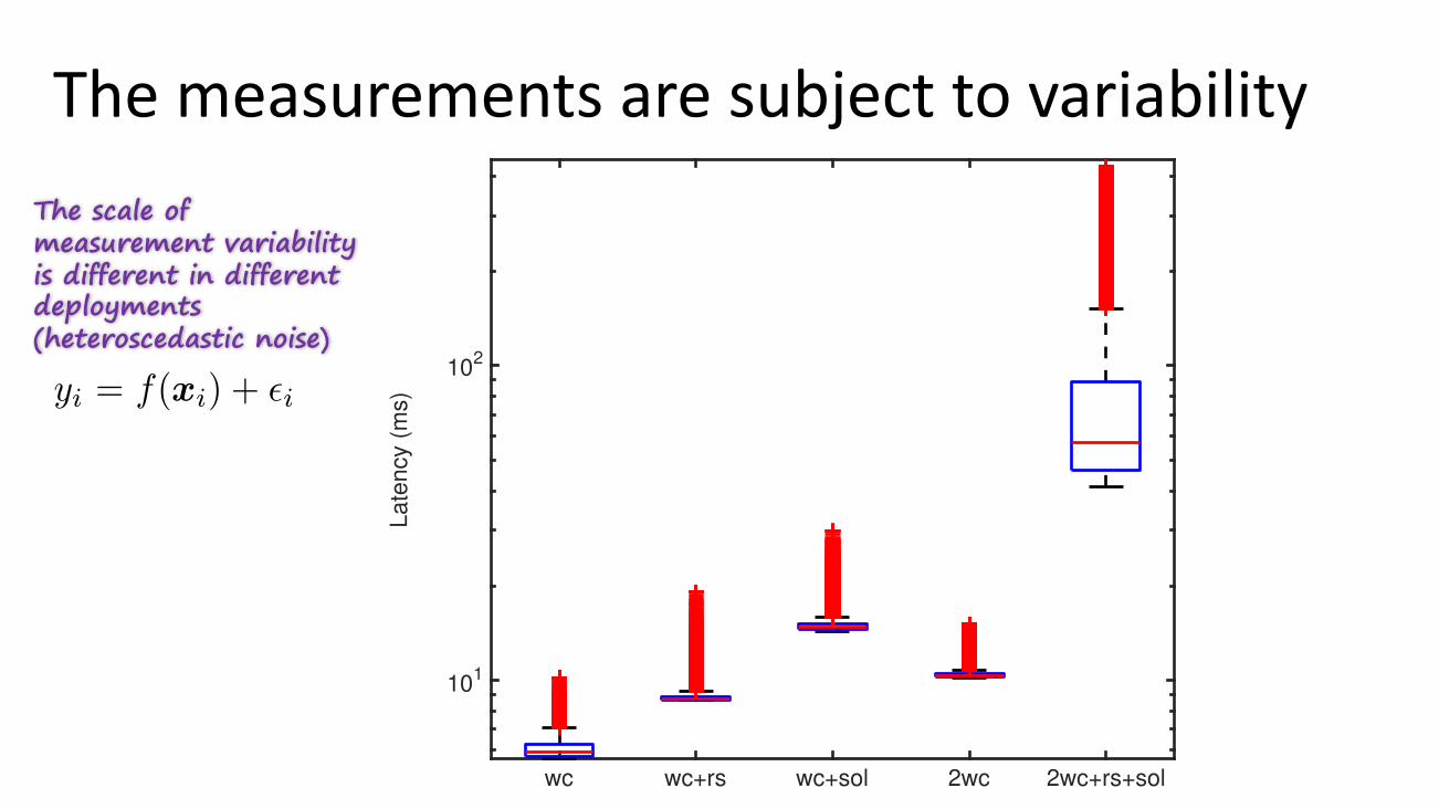
Themeasurementsaresubjecttovariability

wc wc+rs wc+sol 2wc 2wc+rs+sol

101

102

Late

ncy

(m

s)

The scale of measurement variability is different in different deployments (heteroscedastic noise)



Kafka Topic

Stream to Kafka

File(sentence)

(sentence)

(sen

tenc

e)

Fig. 1: WordCount topology architecture.

of d parameters of interest. We assume that each configurationx 2 X is valid and denote by f(x) the response measured onthe SPS under that configuration. Throughout, we assume thatf is latency, however other response metrics (e.g., throughput)may be used. The graph of f over configurations is calledthe response surface and it is partially observable, i.e., theactual value of f(x) is known only at points x that has beenpreviously experimented with. We here consider the problemof finding an optimal configuration x

⇤ that minimizes f overthe configuration space X with as few experiments as possible:

x

⇤= argmin

x2Xf(x) (1)

In fact, the response function f(·) is usually unknown orpartially known, i.e., y

i

= f(xi

),xi

⇢ X. In practice, suchmeasurements may contain noise, i.e., y

i

= f(xi

) + ✏i

. Notethat since the response surface is only partially-known, findingthe optimal configuration is a blackbox optimization problem[23], [29], which is also subject to noise. In fact, the problemof finding a optimal solution of a non-convex and multi-modalresponse surface (cf. Figure 2) is NP-hard [36]. Therefore, oninstances where it is impossible to locate a global optimum,BO4CO will strive to find the best possible local optimumwithin the available experimental budget.

B. Motivation1) A running example: WordCount (cf. Figure 1) is a

popular benchmark SPS. In WordCount a text file is fedto the system and it counts the number of occurrences ofthe words in the text file. In Storm, this corresponds to thefollowing operations. A Processing Element (PE) called Spoutis responsible to read the input messages (tuples) from a datasource (e.g., a Kafka topic) and stream the messages (i.e.,sentences) to the topology. Another PE of type Bolt calledSplitter is responsible for splitting sentences into words, whichare then counted by another PE called Counter.

2) Nonlinear interactions: We now illustrate one of theinherent challenges of configuration optimization. The metricthat defines the surface in Figure 2 is the latency of individualmessages, defined as the time since emission by the KafkaSpout to completion at the Counter, see Figure 1. Note thatthis function is the subset of wc(6D) in Table I when the levelof parallelism of Splitters and Counters is varied in [1, 6] and[1, 18]. The surface is strongly non-linear and multi-modaland indicates two important facts. First, the performancedifference between the best and worst settings is substantial,65%, and with more intense workloads we have observeddifferences in latency as large as 99%, see Table V. Next, non-linear relations between the parameters imply that the optimalnumber of counters depends on the number of Splitters, andvice-versa. Figure 3 shows this non-linear interaction [31] and


late

ncy

(ms)

100

150

1

200

250

2

300


243

684 10

125 14166 18

Fig. 2: WordCount response surface. It is an interpolated sur-face and is a projection of 6 dimensions, in wc(6D), onto 2D.It shows the non-convexity, multi-modality and the substantialperformance difference between different configurations.

0 5 10 15 20Number of counters

100

120

140

160

180

200

220

240

Late

ncy (

ms)

splitters=2splitters=3

Fig. 3: WordCount latency, cut though Figure 2.

demonstrates that if one tries to minimize latency by actingjust on one of these parameters at the time, the resultingconfiguration may not lead to a global optimum, as the numberof Splitters has a strong influence on the optimal counters.

3) Sparsity of effects: Another observation from our ex-tensive experiments with SPS is the sparsity of effects. Morespecifically, this means low-order interactions among a fewdominating factors can explain the main changes in the re-sponse function observed in the experiments. In this work weassume sparsity of effects, which also helps in addressing theintractable growth of the configuration space [19].

Methodology. In order to verify to what degree the sparsityof effects assumption holds in SPS, we ran experimentson 3 different benchmarks that exhibit different bottlenecks:WordCount (wc) is CPU intensive, RollingSort (rs) is mem-ory intensive, and SOL (sol) is network intensive. Differenttestbed settings were also considered, for a total of 5 datasets,as listed in Table I. Note that the parameters we considerhere are known to significantly influence latency, as they havebeen chosen according to professional tuning guides [26] andalso small scale tests where we varied a single parameter tomake sure that the selected parameters were all influential.For each test in the experiment, we run the benchmark for 8minutes including the initial burn-in period. Further detailson the experimental procedure are given in Section IV-B.Note that the largest dataset (i.e., rs(6D)) has required alone3840 ⇥ 8/60/24 = 21 days, within a total experimental timeof about 2.5 months to collect the datasets of Table I.

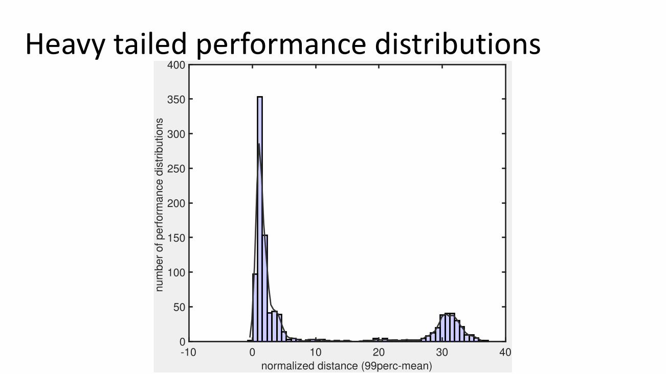
Heavytailedperformancedistributions

-10 0 10 20 30 40normalized distance (99perc-mean)

0

50

100

150

200

250

300

350

400

num

ber

of perf

orm

ance

dis

trib

utio

ns

BO4COarchitecture

Configuration Optimisation Tool

performance repository

Monitoring

Deployment Service

Data Preparation

configuration parameters

values


values

Experimental Suite

Testbed

Doc

Data Broker

Tester

experiment timepolling interval

configurationparameters

GP model

Kafka

System Under TestWorkloadGenerator

Technology Interface

Stor

m

Cas

sand

ra

Spar

k

GPformodelingblackboxresponsefunction

true function

GP mean

GP variance

observation

selected point

true minimum

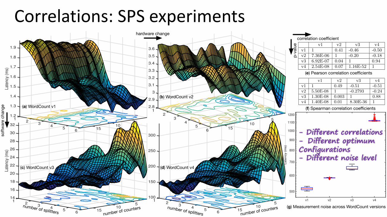
Table 1: Pearson (Spearman) correlation coe�cients.v1 v2 v3 v4

v1 1 0.41 (0.49) -0.46 (-0.51) -0.50 (-0.51)v2 7.36E-06 (5.5E-08) 1 -0.20 (-0.2793) -0.18 (-0.24)v3 6.92E-07 (1.3E-08) 0.04 (0.003) 1 0.94 (0.88)v4 2.54E-08 (1.4E-08) 0.07 (0.01) 1.16E-52 (8.3E-36) 1

Table 2: Signal to noise ratios for WordCount.

Top. µ � µci �ciµ�

wc(v1) 516.59 7.96 [515.27, 517.90] [7.13, 9.01] 64.88wc(v2) 584.94 2.58 [584.51, 585.36] [2.32, 2.92] 226.32wc(v3) 654.89 13.56 [652.65, 657.13] [12.15, 15.34] 48.30wc(v4) 1125.81 16.92 [1123, 1128.6] [15.16, 19.14] 66.56

Figure 2 (a,b,c,d) shows the response surfaces for 4 di↵er-ent versions of the WordCount when splitters and countersare varied in [1, 6] and [1, 18]. WordCount v1, v2 (also v3, v4)are identical in terms of source code, but the environmentin which they are deployed on is di↵erent (we have deployedseveral other systems that compete for capacity in the samecluster). WordCount v1, v3 (also v2, v4) are deployed on a sim-ilar environment, but they have undergone multiple softwarechanges (we artificially injected delays in the source codeof its components). A number of interesting observationscan be made from the experimental results in Figure 2 andTables 1, 2 that we describe in the following subsections.

Correlation across di↵erent versions. We have measuredthe correlation coe�cients between the four versions of Word-Count in Table 1 (upper triangle shows the coe�cients whilelower triangle shows the p-values). The correlations be-tween the response functions are significant (p-values areless than 0.05). However, the correlation di↵ers betweenversions to versions. Also, more interestingly, di↵erent ver-sions of the system have di↵erent optimal configurations:x⇤v1 = (5, 1), x⇤

v2 = (6, 2), x⇤v3 = (2, 13), x⇤

v4 = (2, 16). InDevOps, di↵erent versions of a system will be delivered con-tinuously on daily basis [3]. Current DevOps practices donot systematically use the knowledge from previous versionsfor performance tuning of the current version under test de-spite such significant correlations [3]. There are two reasonsbehind this: (i) the techniques that are used for performancetuning cannot exploit the historical data belong to a di↵erentversion. (ii) they assume di↵erent versions have the sameoptimum configuration. However, based on our experimentalobservations above, this is not true. As a result, the existingpractice treat the experimental data as one-time-use.

Nonlinear interactions. The response functions f(·) in Fig-ure 2 are strongly non-linear, non-convex and multi-modal.The performance di↵erence between the best and worst set-tings is substantial, e.g., 65% in v4, providing a case foroptimal tuning. Moreover, the non-linear relations amongthe parameters imply that the optimal number of countersdepends on splitters, and vice-versa. In other words, if onetries to minimize latency by acting just on one of theseparameters, this may not lead to a global optimum [21].Measurement uncertainty. We have taken samples of the

latency for the same configuration (splitters=counters=1) ofthe 4 versions of WordCount. The experiment were conductedon Amazon EC2 (m3.large (2 CPU, 7.5 GB)). After filteringthe initial burn-in, we have computed average and variance ofthe measurements. The results in Table 2 illustrate that thevariability of measurements across di↵erent versions can beof di↵erent scales. In traditional techniques, such as designof experiments, the variability is typically disregarded byrepeating experiments and obtaining the mean. However, wehere pursue an alternative approach that relies on MTGPmodels that are able to explicitly take into account variability.

3. TL4CO: TRANSFER LEARNING FOR CON-FIGURATION OPTIMIZATION

3.1 Single-task GP Bayesian optimizationBayesian optimization [34] is a sequential design strategy

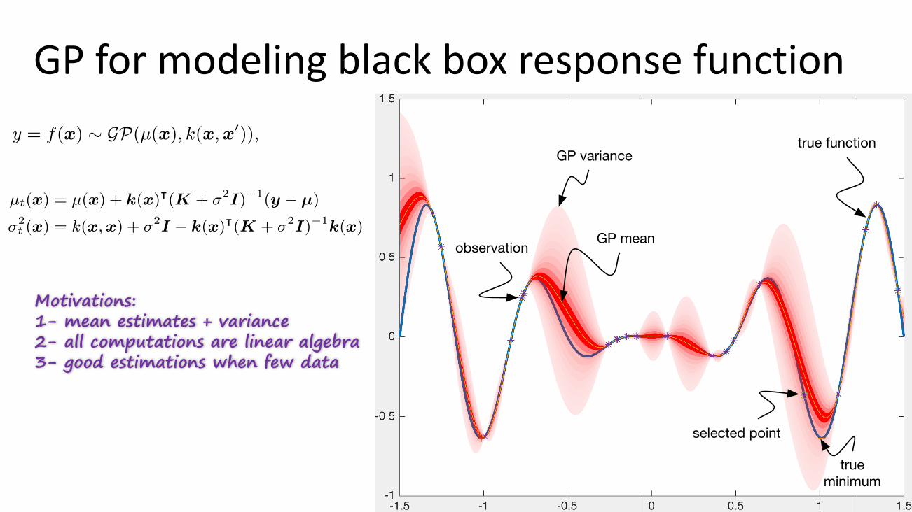
that allows us to perform global optimization of black-boxfunctions. Figure 3 illustrates the GP-based Bayesian Op-timization approach using a 1-dimensional response. Thecurve in blue is the unknown true response, whereas themean is shown in yellow and the 95% confidence interval ateach point in the shaded red area. The stars indicate ex-perimental measurements (or observation interchangeably).Some points x 2 X have a large confidence interval due tolack of observations in their neighborhood, while others havea narrow confidence. The main motivation behind the choiceof Bayesian Optimization here is that it o↵ers a frameworkin which reasoning can be not only based on mean estimatesbut also the variance, providing more informative decisionmaking. The other reason is that all the computations inthis framework are based on tractable linear algebra.In our previous work [21], we proposed BO4CO that ex-

ploits single-task GPs (no transfer learning) for prediction ofposterior distribution of response functions. A GP model iscomposed by its prior mean (µ(·) : X ! R) and a covariancefunction (k(·, ·) : X⇥ X ! R) [41]:

y = f(x) ⇠ GP(µ(x), k(x,x0)), (2)

where covariance k(x,x0) defines the distance between x

and x

0. Let us assume S1:t = {(x1:t, y1:t)|yi := f(xi)} bethe collection of t experimental data (observations). In thisframework, we treat f(x) as a random variable, conditionedon observations S1:t, which is normally distributed with thefollowing posterior mean and variance functions [41]:

µt(x) = µ(x) + k(x)|(K + �2I)�1(y � µ) (3)

�2t (x) = k(x,x) + �2

I � k(x)|(K + �2I)�1

k(x) (4)

where y := y1:t, k(x)| = [k(x,x1) k(x,x2) . . . k(x,xt)],

µ := µ(x1:t), K := k(xi,xj) and I is identity matrix. Theshortcoming of BO4CO is that it cannot exploit the observa-tions regarding other versions of the system and as thereforecannot be applied in DevOps.

3.2 TL4CO: an extension to multi-tasksTL4CO 1 uses MTGPs that exploit observations from other

previous versions of the system under test. Algorithm 1defines the internal details of TL4CO. As Figure 4 shows,TL4CO is an iterative algorithm that uses the learning fromother system versions. In a high-level overview, TL4CO: (i)selects the most informative past observations (details inSection 3.3); (ii) fits a model to existing data based on kernellearning (details in Section 3.4), and (iii) selects the nextconfiguration based on the model (details in Section 3.5).

In the multi-task framework, we use historical data to fit abetter GP providing more accurate predictions. Before that,we measure few sample points based on Latin Hypercube De-sign (lhd) D = {x1, . . . , xn} (cf. step 1 in Algorithm 1). Wehave chosen lhd because: (i) it ensures that the configurationsamples in D is representative of the configuration space X,whereas traditional random sampling [26, 17] (called brute-force) does not guarantee this [29]; (ii) another advantage isthat the lhd samples can be taken one at a time, making it e�-cient in high dimensional spaces. We define a new notation for1Code+Data will be released (due in July 2016), as this isfunded under the EU project DICE: https://github.com/dice-project/DICE-Configuration-BO4CO

3

Table 1: Pearson (Spearman) correlation coe�cients.v1 v2 v3 v4

v1 1 0.41 (0.49) -0.46 (-0.51) -0.50 (-0.51)v2 7.36E-06 (5.5E-08) 1 -0.20 (-0.2793) -0.18 (-0.24)v3 6.92E-07 (1.3E-08) 0.04 (0.003) 1 0.94 (0.88)v4 2.54E-08 (1.4E-08) 0.07 (0.01) 1.16E-52 (8.3E-36) 1

Table 2: Signal to noise ratios for WordCount.

Top. µ � µci �ciµ�

wc(v1) 516.59 7.96 [515.27, 517.90] [7.13, 9.01] 64.88wc(v2) 584.94 2.58 [584.51, 585.36] [2.32, 2.92] 226.32wc(v3) 654.89 13.56 [652.65, 657.13] [12.15, 15.34] 48.30wc(v4) 1125.81 16.92 [1123, 1128.6] [15.16, 19.14] 66.56

Figure 2 (a,b,c,d) shows the response surfaces for 4 di↵er-ent versions of the WordCount when splitters and countersare varied in [1, 6] and [1, 18]. WordCount v1, v2 (also v3, v4)are identical in terms of source code, but the environmentin which they are deployed on is di↵erent (we have deployedseveral other systems that compete for capacity in the samecluster). WordCount v1, v3 (also v2, v4) are deployed on a sim-ilar environment, but they have undergone multiple softwarechanges (we artificially injected delays in the source codeof its components). A number of interesting observationscan be made from the experimental results in Figure 2 andTables 1, 2 that we describe in the following subsections.

Correlation across di↵erent versions. We have measuredthe correlation coe�cients between the four versions of Word-Count in Table 1 (upper triangle shows the coe�cients whilelower triangle shows the p-values). The correlations be-tween the response functions are significant (p-values areless than 0.05). However, the correlation di↵ers betweenversions to versions. Also, more interestingly, di↵erent ver-sions of the system have di↵erent optimal configurations:x⇤v1 = (5, 1), x⇤

v2 = (6, 2), x⇤v3 = (2, 13), x⇤

v4 = (2, 16). InDevOps, di↵erent versions of a system will be delivered con-tinuously on daily basis [3]. Current DevOps practices donot systematically use the knowledge from previous versionsfor performance tuning of the current version under test de-spite such significant correlations [3]. There are two reasonsbehind this: (i) the techniques that are used for performancetuning cannot exploit the historical data belong to a di↵erentversion. (ii) they assume di↵erent versions have the sameoptimum configuration. However, based on our experimentalobservations above, this is not true. As a result, the existingpractice treat the experimental data as one-time-use.

Nonlinear interactions. The response functions f(·) in Fig-ure 2 are strongly non-linear, non-convex and multi-modal.The performance di↵erence between the best and worst set-tings is substantial, e.g., 65% in v4, providing a case foroptimal tuning. Moreover, the non-linear relations amongthe parameters imply that the optimal number of countersdepends on splitters, and vice-versa. In other words, if onetries to minimize latency by acting just on one of theseparameters, this may not lead to a global optimum [21].Measurement uncertainty. We have taken samples of the

latency for the same configuration (splitters=counters=1) ofthe 4 versions of WordCount. The experiment were conductedon Amazon EC2 (m3.large (2 CPU, 7.5 GB)). After filteringthe initial burn-in, we have computed average and variance ofthe measurements. The results in Table 2 illustrate that thevariability of measurements across di↵erent versions can beof di↵erent scales. In traditional techniques, such as designof experiments, the variability is typically disregarded byrepeating experiments and obtaining the mean. However, wehere pursue an alternative approach that relies on MTGPmodels that are able to explicitly take into account variability.

3. TL4CO: TRANSFER LEARNING FOR CON-FIGURATION OPTIMIZATION

3.1 Single-task GP Bayesian optimizationBayesian optimization [34] is a sequential design strategy

that allows us to perform global optimization of black-boxfunctions. Figure 3 illustrates the GP-based Bayesian Op-timization approach using a 1-dimensional response. Thecurve in blue is the unknown true response, whereas themean is shown in yellow and the 95% confidence interval ateach point in the shaded red area. The stars indicate ex-perimental measurements (or observation interchangeably).Some points x 2 X have a large confidence interval due tolack of observations in their neighborhood, while others havea narrow confidence. The main motivation behind the choiceof Bayesian Optimization here is that it o↵ers a frameworkin which reasoning can be not only based on mean estimatesbut also the variance, providing more informative decisionmaking. The other reason is that all the computations inthis framework are based on tractable linear algebra.In our previous work [21], we proposed BO4CO that ex-

ploits single-task GPs (no transfer learning) for prediction ofposterior distribution of response functions. A GP model iscomposed by its prior mean (µ(·) : X ! R) and a covariancefunction (k(·, ·) : X⇥ X ! R) [41]:

y = f(x) ⇠ GP(µ(x), k(x,x0)), (2)

where covariance k(x,x0) defines the distance between x

and x

0. Let us assume S1:t = {(x1:t, y1:t)|yi := f(xi)} bethe collection of t experimental data (observations). In thisframework, we treat f(x) as a random variable, conditionedon observations S1:t, which is normally distributed with thefollowing posterior mean and variance functions [41]:

µt(x) = µ(x) + k(x)|(K + �2I)�1(y � µ) (3)

�2t (x) = k(x,x) + �2

I � k(x)|(K + �2I)�1

k(x) (4)

where y := y1:t, k(x)| = [k(x,x1) k(x,x2) . . . k(x,xt)],

µ := µ(x1:t), K := k(xi,xj) and I is identity matrix. Theshortcoming of BO4CO is that it cannot exploit the observa-tions regarding other versions of the system and as thereforecannot be applied in DevOps.

3.2 TL4CO: an extension to multi-tasksTL4CO 1 uses MTGPs that exploit observations from other

previous versions of the system under test. Algorithm 1defines the internal details of TL4CO. As Figure 4 shows,TL4CO is an iterative algorithm that uses the learning fromother system versions. In a high-level overview, TL4CO: (i)selects the most informative past observations (details inSection 3.3); (ii) fits a model to existing data based on kernellearning (details in Section 3.4), and (iii) selects the nextconfiguration based on the model (details in Section 3.5).

In the multi-task framework, we use historical data to fit abetter GP providing more accurate predictions. Before that,we measure few sample points based on Latin Hypercube De-sign (lhd) D = {x1, . . . , xn} (cf. step 1 in Algorithm 1). Wehave chosen lhd because: (i) it ensures that the configurationsamples in D is representative of the configuration space X,whereas traditional random sampling [26, 17] (called brute-force) does not guarantee this [29]; (ii) another advantage isthat the lhd samples can be taken one at a time, making it e�-cient in high dimensional spaces. We define a new notation for1Code+Data will be released (due in July 2016), as this isfunded under the EU project DICE: https://github.com/dice-project/DICE-Configuration-BO4CO

3

Motivations:1- mean estimates + variance2- all computations are linear algebra3- good estimations when few data

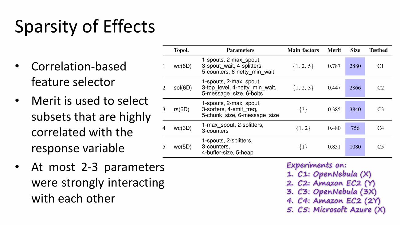
SparsityofEffects

• Correlation-basedfeature selector

• Meritisusedtoselectsubsetsthatarehighlycorrelatedwiththeresponsevariable

• At most 2-3 parameterswere strongly interactingwith each other

TABLE I: Sparsity of effects on 5 experiments where we have varieddifferent subsets of parameters and used different testbeds. Note thatthese are the datasets we experimentally measured on the benchmarksystems and we use them for the evaluation, more details includingthe results for 6 more experiments are in the appendix.

Topol. Parameters Main factors Merit Size Testbed

1 wc(6D)1-spouts, 2-max spout,3-spout wait, 4-splitters,5-counters, 6-netty min wait

{1, 2, 5} 0.787 2880 C1

2 sol(6D)1-spouts, 2-max spout,3-top level, 4-netty min wait,5-message size, 6-bolts

{1, 2, 3} 0.447 2866 C2

3 rs(6D)1-spouts, 2-max spout,3-sorters, 4-emit freq,5-chunk size, 6-message size

{3} 0.385 3840 C3

4 wc(3D) 1-max spout, 2-splitters,3-counters {1, 2} 0.480 756 C4

5 wc(5D)1-spouts, 2-splitters,3-counters,4-buffer-size, 5-heap

{1} 0.851 1080 C5

wc wc+rs wc+sol 2wc 2wc+rs+sol

101

102

Late

ncy

(m

s)

Fig. 4: Noisy experimental measurements. Note that + heremeans that wc is deployed in a multi-tenant environmentwith other topologies and as a result not only the latency isincreased but also the variability became greater.

Results. After collecting experimental data, we have useda common correlation-based feature selector1 implemented inWeka to rank parameter subsets according to a heuristic. Thebias of the merit function is toward subsets that contain pa-rameters that are highly correlated with the response variable.Less influential parameters are filtered because they will havelow correlation with latency, and a set with the main factorsis returned. For all of the 5 datasets, we list in Table I themain factors. The analysis results demonstrate that in all the 5experiments at most 2-3 parameters were strongly interactingwith each other, out of a maximum of 6 parameters variedsimultaneously. Therefore, the determination of the regionswhere performance is optimal will likely be controlled by suchdominant factors, even though the determination of a globaloptimum will still depends on all the parameters.

4) Measurement uncertainty: We now illustrate measure-ment variabilities, which represent an additional challenge forconfiguration optimization. As depicted in Figure 4, we took

1The most significant parameters are selected based on the following meritfunction [9], also shown in Table I:

mps =nrlpp

n+ n(n� 1)rpp, (2)

where rlp is the mean parameter-latency correlation, n is the number ofparameters, rpp is the average feature-feature inter-correlation [9, Sec 4.4].

different samples of the latency metric over 2 hours for fivedifferent deployments of WordCount. The experiments runon a multi-node cluster on the EC2 cloud. After filtering theinitial burn-in, we computed averages and standard deviationof the latencies. Note that the configuration across all 5settings is similar, the only difference is the number of co-located topologies in the testbed. The data in boxplots illustratethat variability can be small in some settings (e.g., wc),while they can be large in some other experimental setups(e.g., 2wc+rs+sol). In traditional techniques such as designof experiments, such variability is addressed by repeatingexperiments multiple times and obtaining regression estimatesfor the system model across such repetitions. However, wehere pursue the alternative approach of relying on GP modelsto capture both mean and variance of measurements withinthe model that guides the configuration process. The theoryunderpinning this approach is discussed in the next section.

III. BO4CO: BAYESIAN OPTIMIZATION FORCONFIGURATION OPTIMIZATION

A. Bayesian Optimization with Gaussian Process prior

Bayesian optimization is a sequential design strategy thatallows us to perform global optimization of blackbox functions[30]. The main idea of this method is to treat the blackboxobjective function f(x) as a random variable with a given priordistribution, and then perform optimization on the posteriordistribution of f(x) given experimental data. In this work,GPs are used to model this blackbox objective function at eachpoint x 2 X. That is, let S1:t be the experimental data collectedin the first t iterations and let x

t+1 be a candidate configurationthat we may select to run the next experiment. Then BO4COassesses the probability that this new experiment could findan optimal configuration using the posterior distribution:

Pr(ft+1|S1:t,xt+1) ⇠ N (µ

t

(x

t+1),�2t

(x

t+1)),

where µt

(x

t+1) and �2t

(x

t+1) are suitable estimators of themean and standard deviation of a normal distribution that isused to model this posterior. The main motivation behind thechoice of GPs as prior here is that it offers a framework inwhich reasoning can be not only based on mean estimatesbut also the variance, providing more informative decisionmakings. The other reason is that all the computations in thisframework are based on linear algebra.

Figure 5 illustrates the GP-based Bayesian optimizationusing a 1-dimensional response surface. The curve in blue isthe unknown true posterior distribution, whereas the mean isshown in green and the 95% confidence interval at each pointin the shaded area. Stars indicate measurements carried out inthe past and recorded in S1:t (i.e., observations). Configurationcorresponds to x1 has a large confidence interval due to lack ofobservations in its neighborhood. Conversely, x4 has a narrowconfidence since neighboring configurations have been exper-imented with. The confidence interval in the neighborhood ofx2 and x3 is not high and correctly our approach does notdecide to explore these zones. The next configuration x

t+1,indicated by a small circle right to the x4, is selected basedon a criterion that will be defined later.

Experiments on:1. C1: OpenNebula (X)2. C2: Amazon EC2 (Y)3. C3: OpenNebula (3X)4. C4: Amazon EC2 (2Y)5. C5: Microsoft Azure (X)

-1.5 -1 -0.5 0 0.5 1 1.5-1.5

-1

-0.5

0

0.5

1

x1 x2 x3 x4

true function

GP surrogate mean estimate

observation

Fig. 5: An example of 1D GP model: GPs provide mean esti-mates as well as the uncertainty in estimations, i.e., variance.



Monitoring

Deployment Service

Data Preparation


values


values

Experimental Suite

Testbed

Doc

Data Broker

Tester



GP model

Kafka



Stor

m

Cas

sand

ra

Spar

k

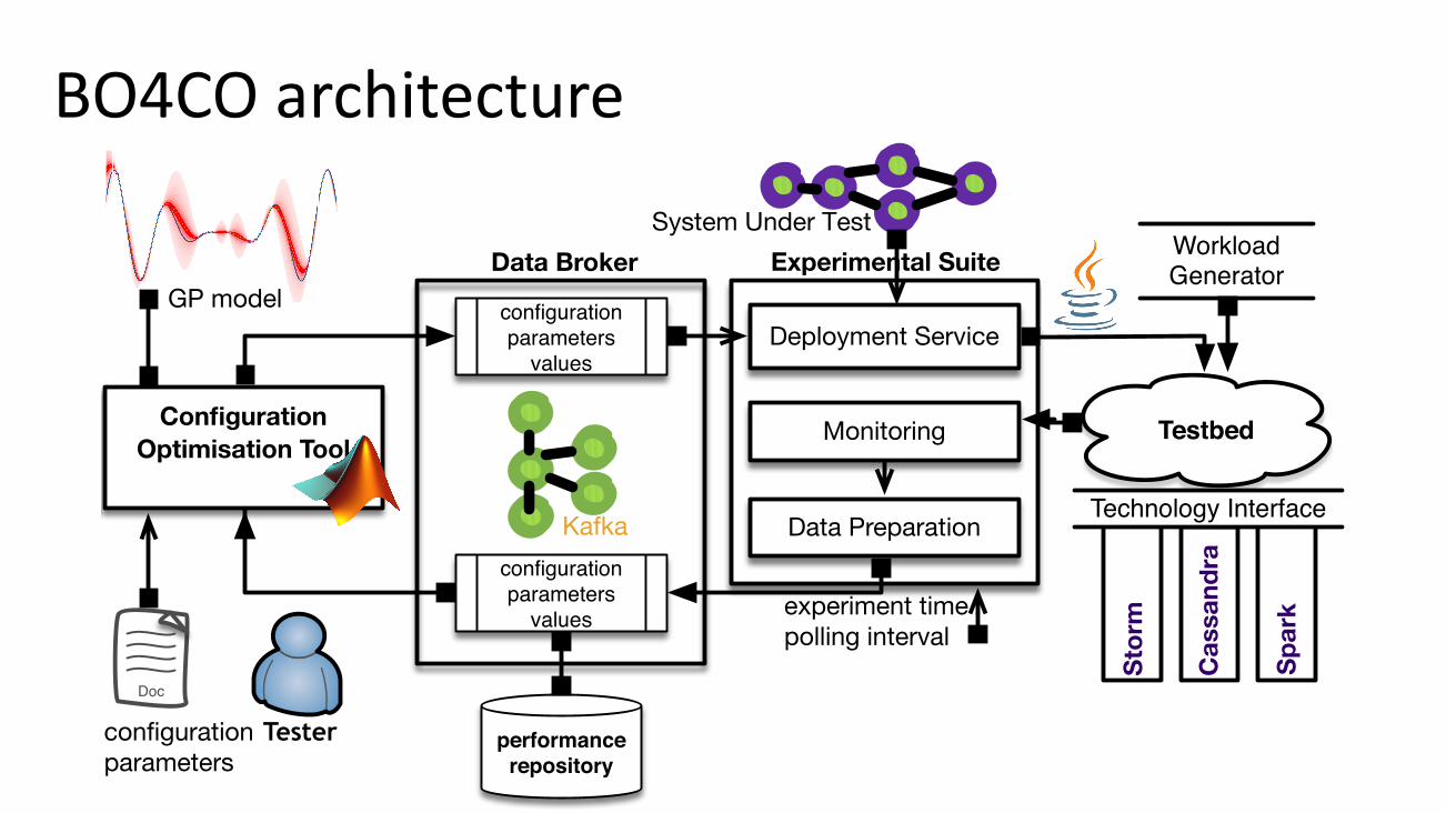
Fig. 6: BO4CO architecture: (i) optimization and (ii) exper-imental suite are integrated via (iii) a data broker. The in-tegrated solution is available: https://github.com/dice-project/DICE-Configuration-BO4CO.

B. BO4CO algorithm

BO4CO’s high-level architecture is shown in Figure 6 andthe procedure that drives the optimization is described in Al-gorithm. We start by bootstrapping the optimization followingLatin Hypercube Design (lhd) to produce an initial designD = {x1, . . . ,xn

} (cf. step 1 in Algorithm 1). Although otherdesign approaches (e.g., random) could be used, we have cho-sen lhd because: (i) it ensures that the configuration samplesin D is representative of the configuration space X, whereastraditional random sampling [17], [9] (called brute-force) doesnot guarantee this [20]; (ii) another advantage is that the lhdsamples can be taken one at a time, making it efficient inhigh dimensional spaces. After obtaining the measurementsregarding the initial design, BO4CO then fits a GP model tothe design points D to form our belief about the underlyingresponse function (cf. step 3 in Algorithm 1). The while loop inAlgorithm 1 iteratively updates the belief until the budget runsout: As we accumulate the data S1:t = {(x

i

, yi

)}ti=1, where

yi

= f(xi

)+ ✏i

with ✏ ⇠ N (0,�2), a prior distribution Pr(f)

and the likelihood function Pr(S1:t|f) form the posteriordistribution: Pr(f |S1:t) / Pr(S1:t|f) Pr(f).

A GP is a distribution over functions [31], specified by itsmean (see Section III-E2), and covariance (see Section III-E1):

y = f(x) ⇠ GP(µ(x), k(x,x0)), (3)

Algorithm 1 : BO4COInput: Configuration space X, Maximum budget N

max

, Re-sponse function f , Kernel function K

✓

, Hyper-parameters✓, Design sample size n, learning cycle N

l

Output: Optimal configurations x

⇤ and learned model M1: choose an initial sparse design (lhd) to find an initial

design samples D = {x1, . . . ,xn

}2: obtain performance measurements of the initial design,

yi

f(xi

) + ✏i

, 8xi

2 D3: S1:n {(x

i

, yi

)}ni=1; t n+ 1

4: M(x|S1:n,✓) fit a GP model to the design . Eq.(3)5: while t N

max

do6: if (t mod N

l

= 0) ✓ learn the kernel hyper-parameters by maximizing the likelihood

7: find next configuration x

t

by optimizing the selectioncriteria over the estimated response surface given the data,x

t

argmaxx

u(x|M, S1:t�1) . Eq.(9)8: obtain performance for the new configuration x

t

, yt

f(x

t

) + ✏t

9: Augment the configuration S1:t = {S1:t�1, (xt

, yt

)}10: M(x|S1:t,✓) re-fit a new GP model . Eq.(7)11: t t+ 1

12: end while13: (x

⇤, y⇤) = min S1:Nmax

14: M(x)

where k(x,x0) defines the distance between x and x

0. Let usassume S1:t = {(x1:t, y1:t)|yi := f(x

i

)} be the collection oft observations. The function values are drawn from a multi-variate Gaussian distribution N (µ,K), where µ := µ(x1:t),

K :=

2

64k(x1,x1) . . . k(x1,xt

)

.... . .

...k(x

t

,x1) . . . k(xt

,xt

)

3

75 (4)

In the while loop in BO4CO, given the observations weaccumulated so far, we intend to fit a new GP model:

f1:tft+1

�⇠ N (µ,

K + �2

I k

k

| k(xt+1,xt+1)

�), (5)

where k(x)

|= [k(x,x1) k(x,x2) . . . k(x,x

t

)] and I

is identity matrix. Given the Eq. (5), the new GP model canbe drawn from this new Gaussian distribution:

Pr(ft+1|S1:t,xt+1) = N (µ

t

(x

t+1),�2t

(x

t+1)), (6)

where

µt

(x) = µ(x) + k(x)

|(K + �2

I)

�1(y � µ) (7)

�2t

(x) = k(x,x) + �2I � k(x)

|(K + �2

I)

�1k(x) (8)

These posterior functions are used to select the next point xt+1

as detailed in Section III-C.

C. Configuration selection criteriaThe selection criteria is defined as u : X ! R that selects

x

t+1 2 X, should f(·) be evaluated next (step 7):

x

t+1 = argmax

x2Xu(x|M, S1:t) (9)

-1.5 -1 -0.5 0 0.5 1 1.5-1

-0.8

-0.6

-0.4

-0.2

0

0.2

0.4

0.6

0.8

1

Configuration Space

Empirical Model

2

4

6

8

10

1212

34

56

160

140

120

100

80

60

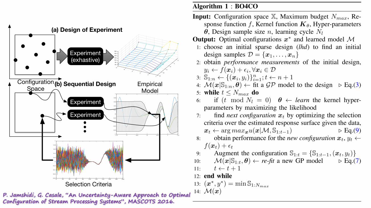
180Experiment(exhastive)

Experiment

Experiment

0 20 40 60 80 100 120 140 160 180 200-0.8

-0.6

-0.4

-0.2

0

0.2

0.4

0.6

0.8

1

Selection Criteria

(b) Sequential Design

(a) Design of Experiment

P. Jamshidi, G. Casale, “An Uncertainty-Aware Approach to Optimal Configuration of Stream Processing Systems”, MASCOTS 2016.

-1.5 -1 -0.5 0 0.5 1 1.5-0.8

-0.6

-0.4

-0.2

0

0.2

0.4

0.6

0.8

configuration domain

resp

onse

val

ue

-1.5 -1 -0.5 0 0.5 1 1.5-0.8

-0.6

-0.4

-0.2

0

0.2

0.4

0.6

0.8

1 true response functionGP fit

-1.5 -1 -0.5 0 0.5 1 1.5-0.8

-0.6

-0.4

-0.2

0

0.2

0.4

0.6

0.8

1

criteria evaluation

new selected point

-1.5 -1 -0.5 0 0.5 1 1.5-0.8

-0.6

-0.4

-0.2

0

0.2

0.4

0.6

0.8

1

new GP fit

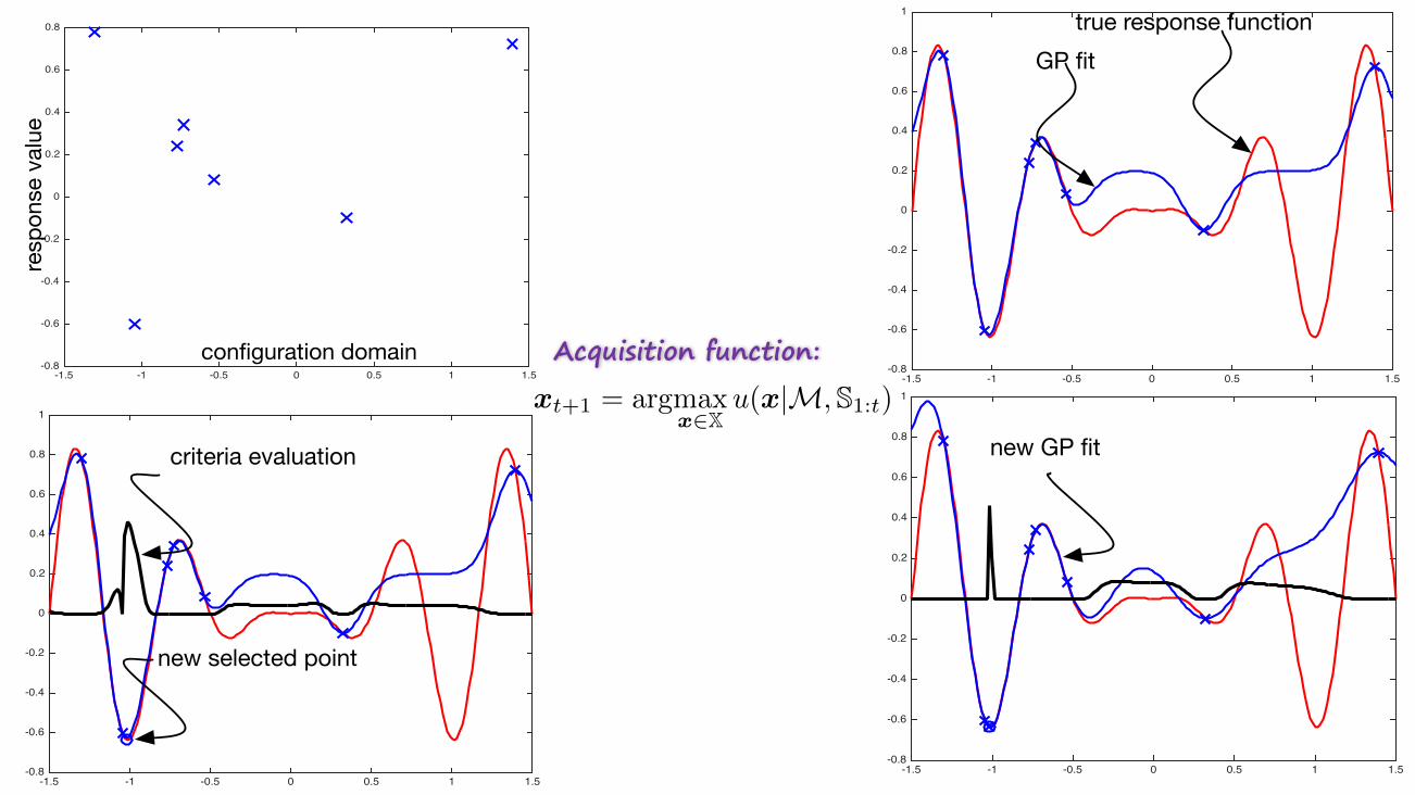
Acquisition function:

-1.5 -1 -0.5 0 0.5 1 1.5-1.5

-1

-0.5

0

0.5

1

x1 x2 x3 x4

true function

GP surrogate mean estimate

observation

Fig. 5: An example of 1D GP model: GPs provide mean esti-mates as well as the uncertainty in estimations, i.e., variance.



Monitoring

Deployment Service

Data Preparation


values


values

Experimental Suite

Testbed

Doc

Data Broker

Tester



GP model

Kafka



Stor

m

Cas

sand

ra

Spar

k

Fig. 6: BO4CO architecture: (i) optimization and (ii) exper-imental suite are integrated via (iii) a data broker. The in-tegrated solution is available: https://github.com/dice-project/DICE-Configuration-BO4CO.

B. BO4CO algorithm

BO4CO’s high-level architecture is shown in Figure 6 andthe procedure that drives the optimization is described in Al-gorithm. We start by bootstrapping the optimization followingLatin Hypercube Design (lhd) to produce an initial designD = {x1, . . . ,xn

} (cf. step 1 in Algorithm 1). Although otherdesign approaches (e.g., random) could be used, we have cho-sen lhd because: (i) it ensures that the configuration samplesin D is representative of the configuration space X, whereastraditional random sampling [22], [11] (called brute-force)does not guarantee this [25]; (ii) another advantage is thatthe lhd samples can be taken one at a time, making it efficientin high dimensional spaces. After obtaining the measurementsregarding the initial design, BO4CO then fits a GP model tothe design points D to form our belief about the underlyingresponse function (cf. step 3 in Algorithm 1). The while loop inAlgorithm 1 iteratively updates the belief until the budget runsout: As we accumulate the data S1:t = {(x

i

, yi

)}ti=1, where

yi

= f(xi

)+ ✏i

with ✏ ⇠ N (0,�2), a prior distribution Pr(f)

and the likelihood function Pr(S1:t|f) form the posteriordistribution: Pr(f |S1:t) / Pr(S1:t|f) Pr(f).

A GP is a distribution over functions [37], specified by itsmean (see Section III-E2), and covariance (see Section III-E1):

y = f(x) ⇠ GP(µ(x), k(x,x0)), (3)

Algorithm 1 : BO4COInput: Configuration space X, Maximum budget N

max

, Re-sponse function f , Kernel function K

✓

, Hyper-parameters✓, Design sample size n, learning cycle N

l

Output: Optimal configurations x

⇤ and learned model M1: choose an initial sparse design (lhd) to find an initial

design samples D = {x1, . . . ,xn

}2: obtain performance measurements of the initial design,

yi

f(xi

) + ✏i

, 8xi

2 D3: S1:n {(x

i

, yi

)}ni=1; t n+ 1

4: M(x|S1:n,✓) fit a GP model to the design . Eq.(3)5: while t N

max

do6: if (t mod N

l

= 0) ✓ learn the kernel hyper-parameters by maximizing the likelihood

7: find next configuration x

t

by optimizing the selectioncriteria over the estimated response surface given the data,x

t

argmaxx

u(x|M, S1:t�1) . Eq.(9)8: obtain performance for the new configuration x

t

, yt

f(x

t

) + ✏t

9: Augment the configuration S1:t = {S1:t�1, (xt

, yt

)}10: M(x|S1:t,✓) re-fit a new GP model . Eq.(7)11: t t+ 1

12: end while13: (x

⇤, y⇤) = min S1:Nmax

14: M(x)

where k(x,x0) defines the distance between x and x

0. Let usassume S1:t = {(x1:t, y1:t)|yi := f(x

i

)} be the collection oft observations. The function values are drawn from a multi-variate Gaussian distribution N (µ,K), where µ := µ(x1:t),

K :=

2

64k(x1,x1) . . . k(x1,xt

)

.... . .

...k(x

t

,x1) . . . k(xt

,xt

)

3

75 (4)

In the while loop in BO4CO, given the observations weaccumulated so far, we intend to fit a new GP model:

f1:tft+1

�⇠ N (µ,

K + �2

I k

k

| k(xt+1,xt+1)

�), (5)

where k(x)

|= [k(x,x1) k(x,x2) . . . k(x,x

t

)] and I

is identity matrix. Given the Eq. (5), the new GP model canbe drawn from this new Gaussian distribution:

Pr(ft+1|S1:t,xt+1) = N (µ

t

(x

t+1),�2t

(x

t+1)), (6)

where

µt

(x) = µ(x) + k(x)

|(K + �2

I)

�1(y � µ) (7)

�2t

(x) = k(x,x) + �2I � k(x)

|(K + �2

I)

�1k(x) (8)

These posterior functions are used to select the next point xt+1

as detailed in Section III-C.

C. Configuration selection criteriaThe selection criteria is defined as u : X ! R that selects

x

t+1 2 X, should f(·) be evaluated next (step 7):

x

t+1 = argmax

x2Xu(x|M, S1:t) (9)

Correlations:SPSexperiments

100

150

1

200

250

Late

ncy

(ms)

300

2 53 104

5 156

14

16

18

20

1

22

24

26

Late

ncy

(ms)

28

30

32

2 53 1045 156 number of countersnumber of splitters number of countersnumber of splitters

2.8

2.9

1

3

3.1

3.2

3.3

2

Late

ncy

(ms)

3.4

3.5

3.6

3 54 10

5 156

1.2

1.3

1.4

1

1.5

1.6

1.7

Late

ncy

(ms)

1.8

1.9

2 53104

5 156

(a) WordCount v1

(b) WordCount v2

(c) WordCount v3 (d) WordCount v4

(e) Pearson correlation coefficients

(g) Measurement noise across WordCount versions

(f) Spearman correlation coefficients

correlation coefficient

p-va

lue

v1 v2 v3 v4

500

600

700

800

900

1000

1100

1200

Late

ncy (

ms)

hardware change

softw

are

chan

ge

Table 1: My caption

v1 v2 v3 v4

v1 1 0.41 -0.46 -0.50

v2 7.36E-06 1 -0.20 -0.18

v3 6.92E-07 0.04 1 0.94

v4 2.54E-08 0.07 1.16E-52 1

Table 2: My caption

v1 v2 v3 v4

v1 1 0.49 -0.51 -0.51

v2 5.50E-08 1 -0.2793 -0.24

v3 1.30E-08 0.003 1 0.88

v4 1.40E-08 0.01 8.30E-36 1

Table 3: My caption

ver. µ � µ�

v1 516.59 7.96 64.88

v2 584.94 2.58 226.32

v3 654.89 13.56 48.30

v4 1125.81 16.92 66.56

1

Table 1: My caption

v1 v2 v3 v4

v1 1 0.41 -0.46 -0.50

v2 7.36E-06 1 -0.20 -0.18

v3 6.92E-07 0.04 1 0.94

v4 2.54E-08 0.07 1.16E-52 1

Table 2: My caption

v1 v2 v3 v4

v1 1 0.49 -0.51 -0.51

v2 5.50E-08 1 -0.2793 -0.24

v3 1.30E-08 0.003 1 0.88

v4 1.40E-08 0.01 8.30E-36 1

Table 3: My caption

ver. µ � µ�

v1 516.59 7.96 64.88

v2 584.94 2.58 226.32

v3 654.89 13.56 48.30

v4 1125.81 16.92 66.56

1

- Different correlations- Different optimum Configurations- Different noise level

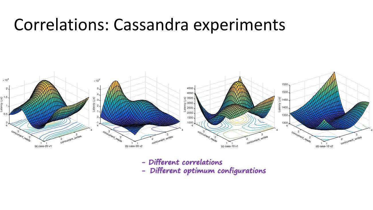
Correlations:Cassandraexperiments

04

0.5

1

4

×104

Late

ncy

(µ

s)

3

1.5

3

2

22

1 1

-14

0

1

2

4

Late

ncy

(µ

s)

×105

3

3

4

3

5

22

1 1

10004

1500

2000

2500

4

3000

Late

ncy

(µ

s)

3

3500

4000

3

4500

22

1 1

13004

1350

1400

4

Late

ncy

(µ

s)

3

1450

1500

3

1550

22

1 1(a) cass-20 v1 (b) cass-20 v2 (c) cass-10 v1 (d) cass-10 v2

concurrent_readsconcurrent_writes




- Different correlations- Different optimum configurations

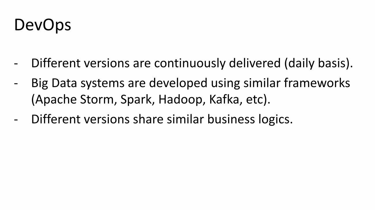
DevOps

- Differentversionsarecontinuouslydelivered(dailybasis).- BigDatasystemsaredevelopedusingsimilarframeworks

(ApacheStorm,Spark,Hadoop,Kafka,etc).- Differentversionssharesimilarbusinesslogics.

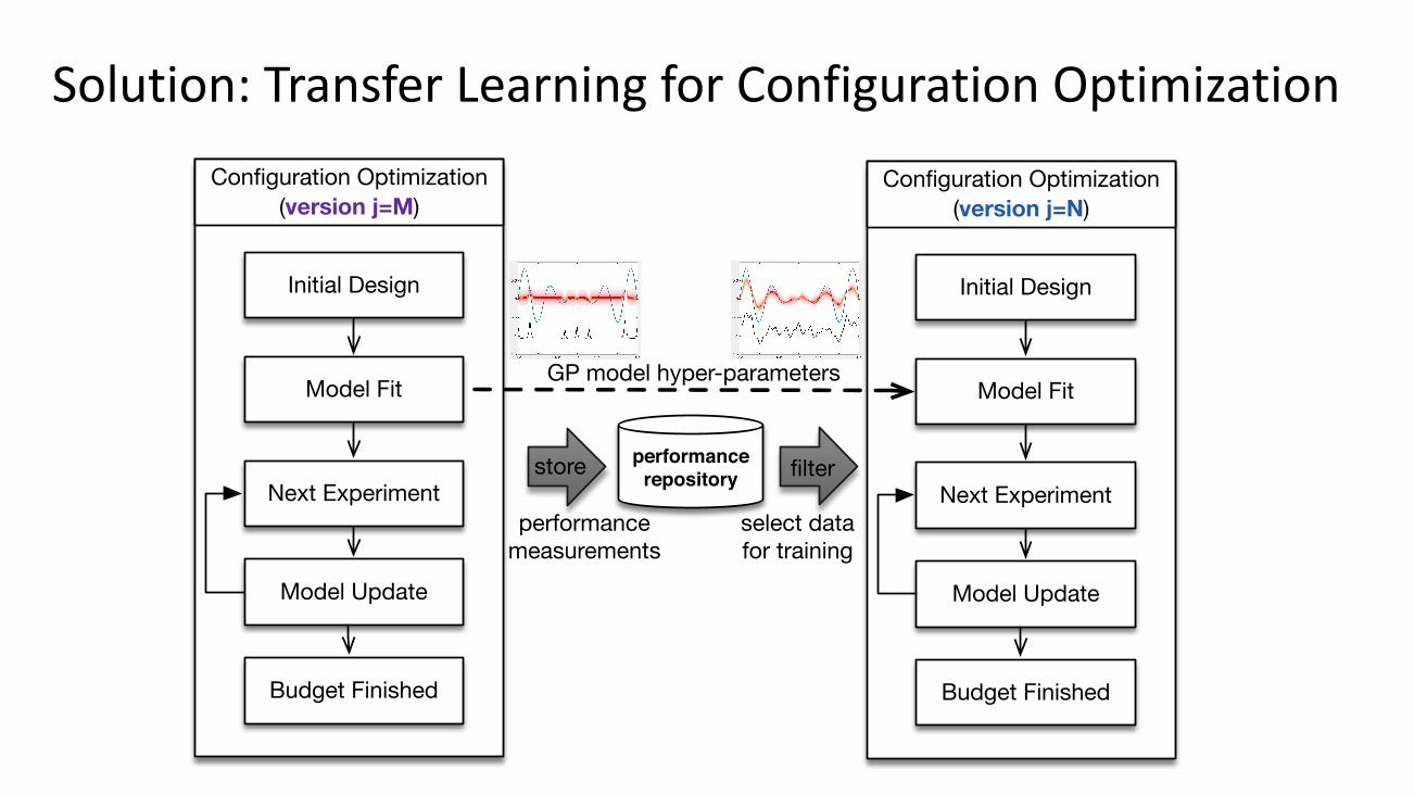
Solution:TransferLearningforConfigurationOptimizationConfiguration Optimization

(version j=M)

performance measurements

Initial Design

Model Fit

Next Experiment

Model Update

Budget Finished


Configuration Optimization(version j=N)

Initial Design

Model Fit

Next Experiment

Model Update

Budget Finished

select data for training

GP model hyper-parameters

store filter

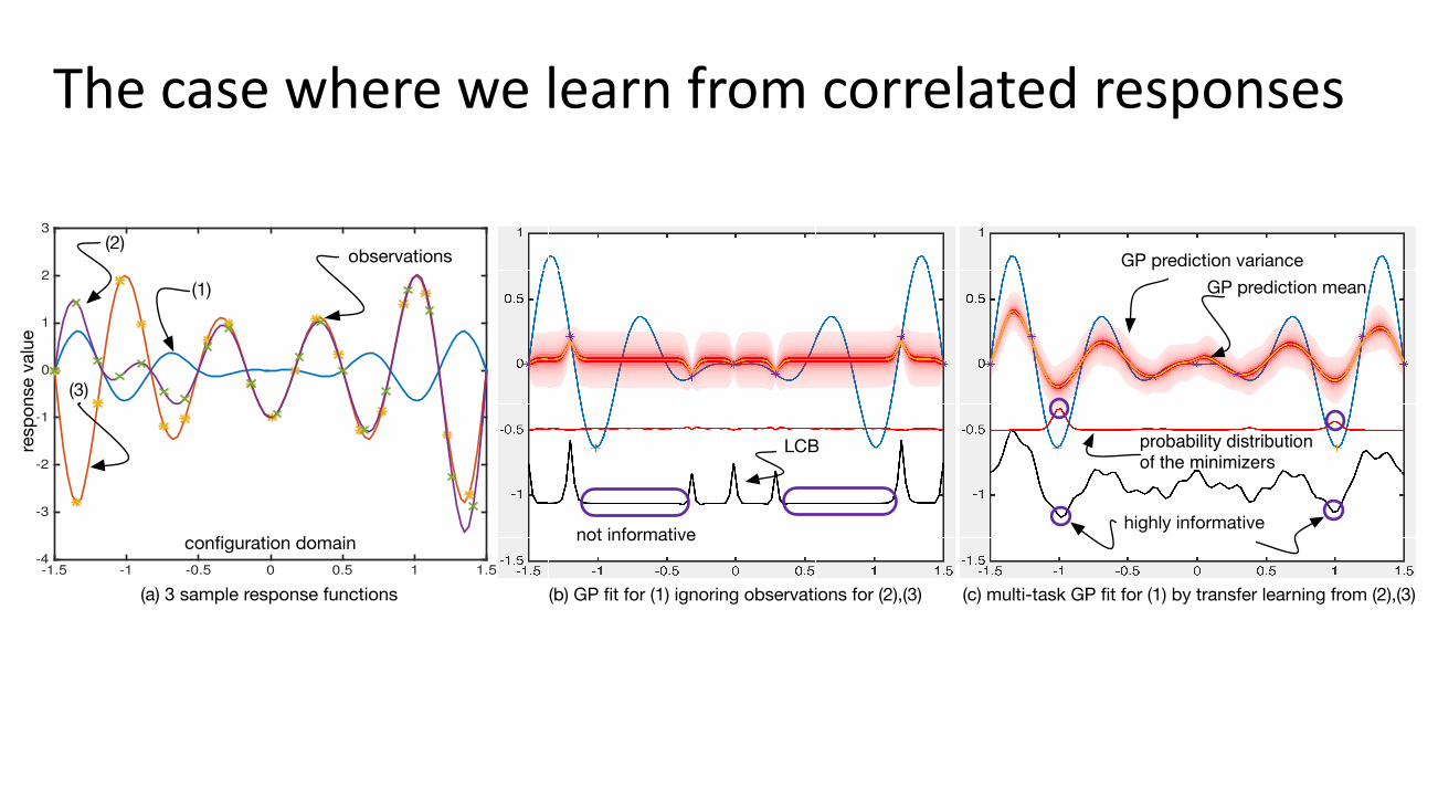
Thecasewherewelearnfromcorrelatedresponses

-1.5 -1 -0.5 0 0.5 1 1.5-4

-3

-2

-1

0

1

2

3

(a) 3 sample response functions

configuration domain

resp

onse

val

ue

(1)

(2)

(3)

observations

(b) GP fit for (1) ignoring observations for (2),(3)

LCB

not informative

(c) multi-task GP fit for (1) by transfer learning from (2),(3)

highly informative

GP prediction meanGP prediction variance

probability distribution of the minimizers

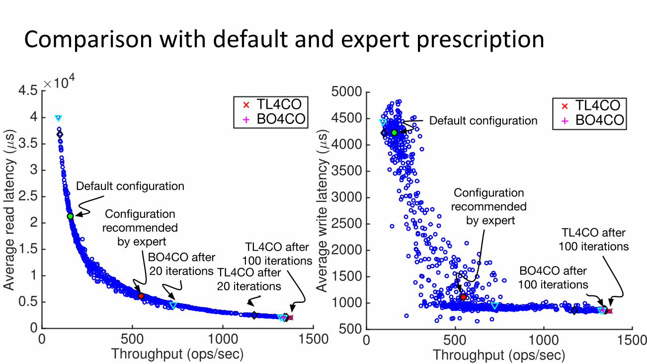
Comparisonwithdefaultandexpertprescription

0 500 1000 1500Throughput (ops/sec)

0

0.5

1

1.5

2

2.5

3

3.5

4

4.5

Ave

rag

e r

ea

d la

ten

cy (µ

s)

×104

TL4COBO4CO

BO4CO after 20 iterations TL4CO after

20 iterations

TL4CO after 100 iterations


500

1000

1500

2000

2500

3000

3500

4000

4500

5000

Ave

rag

e w

rite

late

ncy

(µ

s)

TL4COBO4CO

Default configuration

Configuration recommended

by expertTL4CO after

100 iterations

BO4CO after 100 iterations



by expert

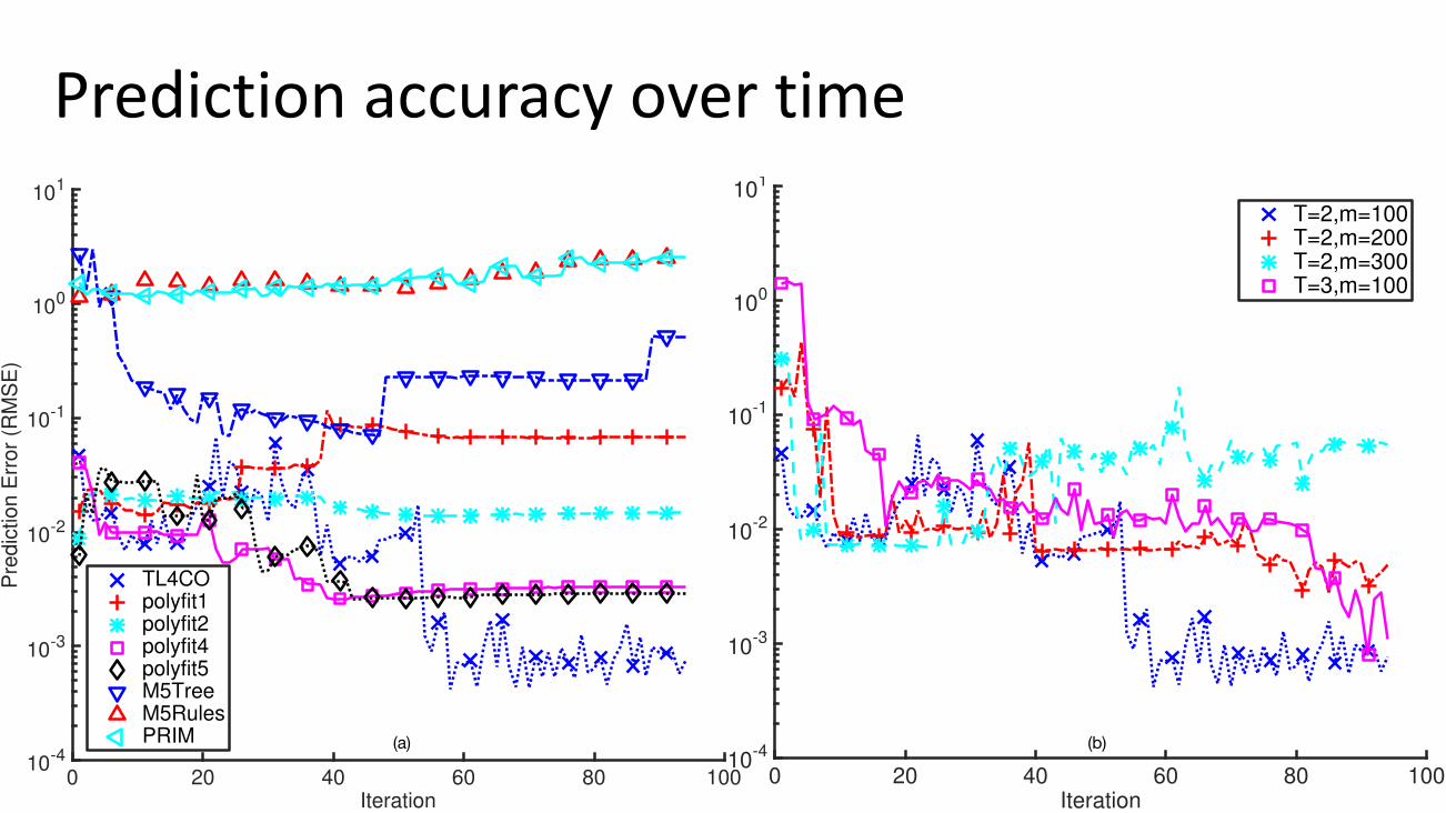
Predictionaccuracyovertime

0 20 40 60 80 100Iteration

10-4

10-3

10-2

10-1

100

101

Pre

dic

tion

Err

or

(RM

SE

)

T=2,m=100T=2,m=200T=2,m=300T=3,m=100

0 20 40 60 80 100Iteration

10-4

10-3

10-2

10-1

100

101

Pre

dic

tion E

rror

(RM

SE

)

TL4COpolyfit1polyfit2polyfit4polyfit5M5TreeM5RulesPRIM (a) (b)

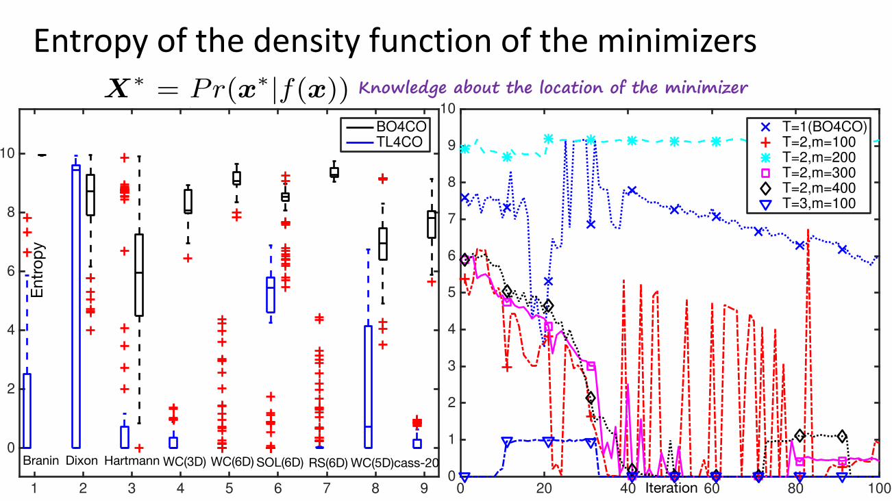
Entropyofthedensityfunctionoftheminimizers

0 20 40 60 80 100Iteration

0

1

2

3

4

5

6

7

8

9

10

Entr

opy

T=1(BO4CO)T=2,m=100T=2,m=200T=2,m=300T=2,m=400T=3,m=100

1 2 3 4 5 6 7 8 9

0

2

4

6

8

10

Entr

opy

BO4COTL4CO

Entro

py

Iteration

Branin Hartmann WC(3D) SOL(6D) WC(5D)Dixon WC(6D) RS(6D) cass-20

0 20 40 60 80 100Iteration (10 minutes each)

101

102

103

104

Abso

lute

Err

or

(µs)

TL4COBO4COSAGAHILLPSDrift

Figure 15: cass-20 configuration optimization.


0

0.5

1

1.5

2

2.5

3

3.5

4

4.5

Ave

rage r

ead la

tency

(µ

s)

×104

TL4COBO4CO

BO4CO after 20 iterations TL4CO after

20 iterations

TL4CO after 100 iterations


500

1000

1500

2000

2500

3000

3500

4000

4500

5000

Ave

rage w

rite

late

ncy

(µ

s)

TL4COBO4CO



by expertTL4CO after

100 iterations

BO4CO after 100 iterations



by expert

Figure 16: TL4CO, BO4CO and expert prescription.

4.5 Entropy analysisThe knowledge about the location of optimum configura-

tion is summarized by the approximation of the conditionalprobability density function of the response function mini-mizers, i.e., X⇤ = Pr(x⇤|f(x)), where f(·) is drawn fromthe MTGP model (cf. solid red line in Figure 5(b,c)). Theentropy of the density functions in Figure 5(b,c) are 6.39,3.96, so we know more information about the latter.

The results in Figure 19 confirm that the entropy measureof the minimizers with the models provided by TL4CO for allthe datasets (synthetic and real) significantly contains moreinformation. The results demonstrate that the main reasonfor finding quick convergence comparing with the baselinesis that TL4CO employs a more e↵ective model. The resultsin Figure 19(b) show the change of entropy of X⇤ over timefor WC(5D) dataset. First, it shows that in TL4CO, theentropy decreases sharply. However, the overall decrease ofentropy for BO4CO is slow. The second observation is thatas we increase the number of observations from similar tasksthe gain in terms of entropy change is not significant. Toshow this more clearly, we have disabled the filtering stepfor T = 2,m = 200 and the results shows that the entropyof X⇤ not only decreases, but it slightly increases over time.

4.6 Computational and memory requirementsThe inference complexity in TL4CO is O(T 2t2) because

of the Cholesky kernel inversion in (6). Since in TL4CO welearn the hyper-parameters every N` iterations, Choleskydecomposition must be re-computed. Therefore the com-plexity is in principle O(T 2t2 ⇥ t/N`). Figure 20(a) providesthe runtime overhead of TL4CO. The time is measured on aMacBook Pro with 2.5 GHz Intel Core i7 CPU and 16GB ofMemory. The computation time in larger datasets (RS(6D),SOL(6D), WC(6D)) is higher than those with less data andlower dimensions (WC(3,5D)). Moreover, the computationtime increases over time since the matrix size for Choleskyinversion gets larger. Figure 20(b) shows the mean and vari-ance of response time over 100 iterations for di↵erent numberof tasks and historical observations per task.

TL4CO polyfit1 polyfit2 polyfit3 polyfit4 polyfit5

10-12

10-10

10-8

10-6

10-4

10-2

100

102

Abso

lute

Perc

enta

ge E

rror

[%]

TL4CO BO4CO M5Tree R-Tree M5Rules MARS PRIM

10-2

10-1

100

101

102

Abso

lute

Perc

enta

ge E

rror

[%]

Abso

lute

Per

cent

age

Erro

r [%

]

Figure 17: Absolute percentage error of predictions made byTL4CO’s MTGP vs regression models for cass-20(6D).

0 20 40 60 80 100Iteration

10-4

10-3

10-2

10-1

100

101

Pre

dic

tion

Err

or

(RM

SE

)

T=2,m=100T=2,m=200T=2,m=300T=3,m=100

0 20 40 60 80 100Iteration

10-4

10-3

10-2

10-1

100

101

Pre

dic

tion

Err

or

(RM

SE

)

TL4COpolyfit1polyfit2polyfit4polyfit5M5TreeM5RulesPRIM (a) (b)

Figure 18: (a) comparing prediction accuracy of TL4CO withother regression models, (b) comparing prediction accuracyof TL4CO with di↵erent number of tasks and observations.

TL4CO requires to store 3 vectors of size |X| = N for mean,variance, and LCB estimates and matrix of size Tn⇥ Tn forstoring K and Tn for keeping tack of historical observations,making the memory requirement O(3N + Tn⇥ Tn+ Tn)).

5. DISCUSSIONS

5.1 Behind the sceneTL4CO in practice: usability and extensibility. In our

experiments, we have evaluated whether TL4CO is feasible inpractice. Although partly parallelized, we have invested morethan three months (24/7) for performance measurements ofthe systems in Table 3 to obtain a huge data basis. However,our approach would require much less measurements, as mostmeasurements were meant to evaluate our approach.

TL4CO can be also used in a di↵erent scenario for configu-ration tuning of Big Data software. Let us assume that thecurrent version of the system is expensive to test (e.g., hasa very large database and each round of experiments takesseveral hours [10]). We, therefore, use a smaller scale of thecurrent version (e.g., with only few records of representativedata). The idea is to spend larger portion of the budget tocollect data from the cheaper version. This data can then beexploited to accelerate the tuning of the expensive version.TL4CO is easy to use, end users only need to determine

the parameters of interests as well as experimental param-eters and then the tool automatically sets the optimizedparameters for the system in its configuration file (all inYAML format). Currently, TL4CO supports Apache Stormand Cassandra. However, it is designed to be extensible, seethe technology interface in Figure 7.How much did ARD help? TL4CO uses ARD technique

(see Section 3.4.1) in order to get a better MTGP fit in statespaces where a subset of parameters interact [21]. To comparethe e↵ects of this technique, we disable ARD for optimization

9

Knowledge about the location of the minimizer

LetsdiscussØ BeawareofUncertainty

- Byquantifying theuncertainty(lookatCatia’s work)- Makedecisionstakingintoaccounttherightlevelofuncertainty(homoscedasticvs

heteroscedastic)- Uncertaintysometimeshelps(modelsthatprovideanestimationoftheuncertainty

aretypicallymoreinformative)- Byexploitingthisknowledgeyoucanonlyexploreinterestingzonesratherthan

learningthewholeperformancefunction

Ø Youcanlearnfromoperationaldata- Notonlyfromthecurrentversion,butfrompreviousmeasurementsaswell- Usethelearningfrompastmeasurementsaspriorknowledge- Toomuchdata canbealsoharmful,itwouldslowdownorblurtheproperlearning

SubmittoSEAMS2017

- AnyworkonSelf-*- ForPerformance-AwareDevOpscommunity:

- DevOpsforadaptivesystems?- Self-adaptiveDevOpspipeline?

- AbstractSubmission:6Jan,2017(firm)- PaperSubmission:13Jan,2017(firm)- Pagelimit:

- Long:10+2,- Newideasandtools:6+1

- Moreinfo:https://wp.doc.ic.ac.uk/seams2017/- Symposium:22-23May,2017- Weacceptartifactssubmissions(tool,data,model)

12thInternationalSymposiumonSoftwareEngineeringforAdaptiveandSelf-ManagingSystems

http://wp.doc.ic.ac.uk/seams2017

CallforPapersSelf-adaptationand self-managementarekeyobjectives inmanymodernandemerging software systems, includingtheindustrialinternetofthings,cyber-physicalsystems,cloudcomputing,andmobilecomputing.Thesesystemsmustbeabletoadaptthemselvesatruntimetopreserveandoptimizetheiroperationinthepresenceofuncertainchangesintheiroperatingenvironment,resourcevariability,newuserneeds,attacks,intrusions,andfaults.

Approachestocomplementsoftware-basedsystemswithself-managingandself-adaptivecapabilitiesareanimportantareaof researchanddevelopment,offeringsolutions that leverageadvances in fieldssuchassoftwarearchitecture,fault-tolerant computing, programming languages, robotics, and run-time program analysis and verification.Additionally, research in this field is informed by related areas like biologically-inspired computing, artificialintelligence,machinelearning,controlsystems,andagent-basedsystems.TheSEAMSsymposiumfocusesonapplyingsoftwareengineeringtotheseapproaches,includingmethods,techniques,andtoolsthatcanbeusedtosupportself-*propertieslikeself-adaptation,self-management,self-healing,self-optimization,andself-configuration.

TheobjectiveofSEAMS is tobring together researchersandpractitioners fromdiverseareas to investigate,discuss,andexaminethefundamentalprinciples,stateoftheart,andcriticalchallengesofengineeringself-adaptiveandself-managingsystems.

TopicsofInterest:Alltopicsrelatedtoengineeringself-adaptiveandself-managingsystems,including:FoundationalConcepts• self-*properties• controltheory• algorithms• decision-makingandplanning• managinguncertainty• mixed-initiativeandhuman-in-the-loopsystems

Languages• formalnotationsformodelingandanalyzingself-*

properties• programminglanguagesupportforself-adaptation

Constructivemethods• requirementselicitationtechniques• reusesupport(e.g.,patterns,designs,code)• architecturaltechniques• legacysystems

AnalyticalMethodsforSelf-Adaptationand-Management• evaluationandassurance• verificationandvalidation• analysisandtestingframeworks

ApplicationAreas• Industrialinternetofthings• Cyber-physicalsystems• Cloudcomputing• Mobilecomputing• Robotics• Smartuserinterfaces• Securityandprivacy• Wearablesandubiquitous/pervasivesystems

Artifacts*andEvaluations• modelproblemsandexemplars• resources,metrics,orsoftwarethatcanbeusedto

compareself-adaptiveapproaches• experiencesinapplyingtoolstorealproblems

*Therewillbeaspecificsessiontobededicatedtoartifactsthatmaybeusefulforthecommunityasawhole.Pleaseseehttp://wp.doc.ic.ac.uk/seams2017/call-for-artifacts/formoredetails.

SelectedpaperswillbeinvitedtosubmittotheACMTransactionsonAutonomousandAdaptiveSystems(TAAS).

PaperSubmissionDetails

FurtherInformationSymposia-relatedemailshouldbeaddressedto:[email protected]

ImportantDates:AbstractSubmission:6January,2017(firm)PaperSubmission:13January,2017(firm)Notification:21February,2017Cameraready:6Mar,2017

SEAMSsolicitsthreetypesofpapers:longpapers(10pagesforthemaintext,inclusiveoffigures,tables,appendices,etc.;referencesmaybeincludedonuptotwoadditionalpages),shortpapersfornewideasandearlyresults(6pages+1references)andartifactpapers(6pages+1reference).Longpapersshouldclearlydescribeinnovativeandoriginalresearchorexplainhowexistingtechniqueshavebeenappliedtoreal-worldexamples.Shortpapersshoulddescribenovelandpromisingideasand/ortechniquesthatareinanearlystageofdevelopment.Artifactpapersmustdescribewhy and how the accompanying artifact may be useful for the broader community. Papers must not have beenpreviously published or concurrently submitted elsewhere. Papersmust conform to IEEE formatting guidelines (seeICSE2017styleguidelines),andsubmittedviaEasyChair.Acceptedpaperswillappear inthesymposiumproceedingsthatwillbepublishedintheACMandIEEEdigitallibraries.

GeneralChairDavidGarlan,USA

ProgramChairBasharNuseibeh,UK

ArtifactChairJavierCámara,US

PublicityChairPooyanJamshidi,UK

LocalChairNicolásD’Ippolito,AR

ProgramCommitteeTBDSteeringCommitteeLucianoBaresi,ItalyNellyBencomo,UKGregorEngels,GermanyRogériodeLemos,UKDavidGarlan,USAPaolaInverardi,ItalyMarinLitoiu(Chair),CanadaJohnMylopoulos,ItalyHausiA.Müller,CanadaBasharNuseibeh,UKBradleySchmerl,USA

Co-lo

cate

d w

ith

Acknowledgement/IC4activities- MyparticipationtotheDagstuhl seminarisfullysupportedbyIC4.- Weareworkingonamachinelearningworkforpredictingthe

performance(jobcompletiontime,utilizations,throughput,performanceregressions)ofbigdata(ApacheHadoopandSpark),theresultswillbesoonpublished(PIs:TheoLynn,BrianLee,andothercolleaguesSaulGill,Binesh Nair,DavidO’Shea,Yuansong Qiao)

- Wearealsoworkingoncloud/microservices migrationforIC4industrymembers(PIs:TheoLynn,ClausPahl)

- Andaself-configurationtoolforhighlyconfigurablesystems(withTheoLynn)