Embed Size (px)
Citation preview

Asieh Abolpour Mofrad
OsloMet Avhandling 2021 nr 3
When Behavior Analysis Meets Machine LearningFormation of Stimulus Equivalence Classes and AdaptiveLearning in Artificial Agents


When Behavior Analysis Meets Machine Learning
Formation of Stimulus Equivalence Classes and Adaptive Learning in
Artificial Agents
Asieh Abolpour Mofrad
Dissertation for the degree of philosophiae doctor (PhD)
Department of Behavioral Science
Faculty of Health Sciences
OsloMet - Oslo Metropolitan University
Spring 2021

CC‐BY‐SA versjon 4.0 OsloMet Avhandling 2021 nr 3 ISSN 2535-471X (trykket) ISSN 2535-5454 (online) ISBN 978-82-8364-282-7 (trykket) ISBN 978-82-8364-292-6 (online) OsloMet – storbyuniversitetet Universitetsbiblioteket Skriftserien St. Olavs plass 4, 0130 Oslo, Telefon (47) 64 84 90 00 Postadresse: Postboks 4, St. Olavs plass 0130 Oslo Trykket hos Byråservice Trykket på Scandia 2000 white, 80 gram på materiesider/200 gram på coveret

Dedicated with love to my parents Sedigheh & Mahmoud,
my sister Samaneh,
and my husband Iman

Preface
This thesis is submitted in partial fulfillment of the requirements for the degree of Philosophiae
Doctor at the University of OsloMet - Oslo Metropolitan University. The research pre-
sented here was conducted at OsloMet Artificial Intelligence (AI) Lab as well as the
Experimental Studies of Complex Human Behaviour (ESCo HuB) Lab, under the super-
vision of Prof. Anis Yazidi (main supervisor), Prof. Erik Arntzen, and Prof. Hugo L.
Hammer.
The thesis is a collection of four theoretical papers, the common theme of which is
computational explanations of behavioral processes with a focus on developing tools for
the study of human behavior in simple yet powerful computational simulations. The
papers are preceded by an introductory chapter that bonds them together and provides
background information and motivation for the work. The candidate is the first author
and corresponding author for the first three papers, and the second author with equal
contribution with professor Anis Yazidi for the last paper. This work was supported by
the OsloMet through grant number 160139.

Acknowledgements
During the journey that led to this dissertation, many wonderful people have helped me.
The few paragraphs below are an attempt to express my deepest gratitude to all those
who made this experience possible.
My utmost gratitude goes to my main supervisor Prof. Anis Yazidi. I am truly
honored to have the opportunity to work with Anis, who is not only a great advisor and
a brilliant researcher but also a trustworthy friend with whom I could share my concerns
and thoughts freely. Beyond his valuable academic advice about research problems, he
has taught me how to be an effective, patient, and confident researcher. I am particularly
thankful to Anis for his trust in my ability and for supporting me to pursue my research
interests. I also appreciate his eagerness to discuss new ideas, thoughts, and methods.
Anis put maximum efforts into facilitating my research stay at the Center for Mind,
Brain, and Computation at Stanford; a visit which was sadly canceled due to the Covid-
19 situation. Finally, I thank him for his constant support during my PhD to follow high
educational and research standards, and his continuous concern regarding my forthcoming
career.
Next, I would like to thank my supervisor, the renowned behavior analyst, Prof. Erik
Arntzen who introduced me to the exciting research area of stimulus equivalence. I have
had the opportunity of acquaintance with experimental methods of behavior analysis and
psychology in his Experimental Studies of Complex Human Behavior (ESCo HuB) Lab.
It was a great honor to become familiar with Erik, cooperate with and learn from him
during my Ph.D. period. I sincerely thank Erik for kindly supporting me to adopt a
distinctive approach regarding the formation of stimulus equivalence classes. Finally, I
would like to especially thank him for his kind supports during the final stages of my
study to overcome the difficulties generated by Covid-19 pandemic.
I would like to thank Prof. Hugo L. Hammer, my advisor at the Computer Science
Department and AI Lab. I benefited from his expertise in many areas, including statistical
parts of my research. His structured way of thinking and well-timed feedbacks helped me
quite often, especially during the first stages of my work, where I was exploring the value
of data and simulation results. I appreciate his constructive attitude, and all I learned
from him during my Ph.D. at OsloMet.
I would like to extend my deepest gratitude to Prof. Jay L. McClelland at the De-

partment of Psychology, Stanford for giving me motivation, excitement, and confidence.
I received these through frequent communications with him and his invitation letter to be
a Visiting Student Scholar (VSR) at his Lab. His responsible attitude toward the hassles
which deprived me of the research stay, clearly proves that not only he is a distinguished
scientist, but also a person with a kind heart. Besides Anis, Jay, and Erik, I would like to
thank all who have been involved in my planned visit at Stanford: Siri Aanstad, Anders
Braarud Hanssen, Mari Devik, Laurence Marie Anna Habib, Tale Skjølsvik, Birgit Abfal-
terer, Richard Buzurgmehr Rahmatulloev, Hilde Tverseth, Guro Fjellstad Stensvag, and
Renee Rittler.
My particular thanks go to the head of the Computer Science Department, Laurence
Marie Anna Habib; she has always been supportive and solution-oriented. Besides, I
thank all the administrative staff working at Computer Science and Behavioural Sciences
Departments. They facilitated the accomplishment of my doctoral degree at OsloMet.
I am also grateful to the present and former members of the Computer Science Depart-
ment and AI Lab for creating a friendly and enjoyable environment. I especially extend
my gratitude to the Ph.D. candidates who shaped numerous memorable occasions during
my study: Habib Sherkat, Roza Abolghasemi, Ramtin Aryan, Desta Haileselassie Hagos,
Ashish Rauniyar, Anna Nishchyk, Sidney Pontes-Filho, Marco Antonio Pinto-Orellana,
Way Kiat Bong, Martha Risnes, Mirjam Mellema, Bineeth Kuriakose, Akriti Sharma, and
my fantastic office-mate and friend Kristine Heiney. Thank you all for serious technical
and research-related dialogues in addition to cheerful everyday communications. I also
thank the Ph.D. candidates at ESCo HuB Lab and the participants in PHBA8100 and
PHBA8110 courses in 2017. Attending the Lab sessions and courses at the Behavioural
Sciences Department was a memorable occasion!
I take this opportunity to thank Mahdi Rouzbahaneh for his comments on the Python
code in Study II and for generously writing a graphical user-friendly interface for EPS
simulator. I also thank Kristin Solli at the unit for Academic Language and Practice for
all the Informative and enjoyable courses they offer. Especially the digital course “Writing
the Introduction to Article-based Dissertations” was motivating; it carried on during the
difficult time of stay-at-home due to Covid-19 and write-your-thesis due to the submission
deadline! I appreciate Kristin to generously read and comment on my thesis introduction
at the end of the course.

I am also thankful to the committee members who kindly accepted to take some
time off their busy schedule near the end of the year to read my thesis and comment
on it: Dr. Angel Eugenio Tovar Y Romo, and Dr. Boudour Ammar. I also thank the
Committee chair Dr. Sigmund Eldevik, the leader of the public defense and head of
Behavioural Sciences Department Prof. Magne Arve Flaten, in addition to senior advisor
Birgit Abfalterer for coordinating administrative parts of my Ph.D. and defense.
Above all, I express my heartfelt gratitude to my parents, for all the support, love,
and meaning they have gifted to me throughout my life. Beyond any doubt, they have
always been sincere consultants whose wise manners of living continue to inspire me.
They have also been an everlasting source of peace and happiness in my life. I feel greatly
thankful for having my parents, my brothers Sajad and Khosrow, my sister Samaneh, my
sister-in-law Ghazal, and my kind husband Iman, for their unconditional everlasting love,
inspiration, support, and encouragement.
I have to express my deepest gratitude to my sister Samaneh for being one of the most
influential people in my life. It is a great privilege and source of happiness to have such a
smart, kind, courage, thoughtful, motivated, and strong person as a caring sister by my
side. I would like to sincerely thank her for being one of the co-authors in Study II of this
thesis, which makes the resulted paper stronger, and the writing process more pleasant.
And last but not the least, my special thanks go to my husband Iman who has always
been a caring, patient fellow. This was great to simultaneously initiate my OsloMet
Ph.D. and marital life with Iman. He encourages me to face difficulties, cross borders of
the habitual, and welcome unknown opportunities for academic research and professional
life. We were forced to spend most of our holidays on my Ph.D. ambition. Regardless, his
cheerfulness to assist me realizing my objectives has always eased the path of hard working.
Thanks for your hopeful correspondence, delicate roses, and mindful companionship Iman!
Asieh Abolpour Mofrad
Oslo, January 2021

“The purpose of (scientific) computing is insight, not numbers.”
Richard Hamming

Abstract
In this thesis, two well studied subjects in behavior analysis are computationally modeled;
formation of stimulus equivalence classes, and adaptive learning. The former is addressed
in Study I and Study II, while the latter is addressed in Study III and Study IV.
Background. Stimulus equivalence as a behavioral analytic approach studies cognitive
skills such as memory and learning. Despite its importance in experimental studies, from
a computational modelling point of view, the formation of stimulus equivalence classes
has largely been under-investigated. On the other hand, adaptive learning in a broad
sense, is a tool to study several cognitive tasks including memory and remembering. An
appropriate model can be used as a cognitive level finder, and as a recommendation tool
to optimize the training and learning sequence of tasks.
Aims. To propose computational models that replicate formation of stimulus equiva-
lence classes and adaptive learning. The models are supposed to be simple, flexible and
interpretable in order to be suitable for analysis of human complex behavior.
Methods. Agents endowed with Reinforcement learning, more precisely Projective Sim-
ulation and Stochastic Point Location, are used to model the interaction between exper-
imenter and the participant through the testing/learning process. Formation of derived
relations in Study I is achieved by on demand computation during the test phase trials
using likelihood reasoning. In Study II, subsequent to the training phase, an iterative dif-
fusion process called Network Enhancement is used to form derived relations, which turns
the test phase into a memory retrieval phase. The solution to Stochastic Point Location
in Study III aims to estimate the tolerable task difficulty level in an online and interactive
settings. In Study IV, the appropriate task difficulty for training and learning is sought by
using a target success rate that is usually defined beforehand by the experimenter using
a method called Balanced Difficulty Task Finder.
Results. The proposed models for replication of equivalence relations, called Equiva-
lence Projective Simulation (Study I) and Enhanced Equivalence Projective Simulation
(Study II) could replicate a variety of settings in a matching-to-sample procedure. The
models are quite flexible and appropriate to replicate results from real experiments and
simulate different scenarios before performing an empirical experiment involving human
subjects. In Study III, we suggest a new method to estimate the unknown point location
in the Stochastic Point Location problem domain using the mutual probability flux con-

cept and we prove that the proposed solution outperforms the legacy solution reported
in the literature. The probability of receiving correct response from the participant is
also estimated as a measure of reliability of participant’s performance. In Study IV, we
propose a model that is able to suggest a manageable difficulty level to a learner based
on online feedback via an asymmetric adjustment technique of difficulty.
Discussion. We aimed for models that are flexible, interpretative without a need of ex-
tensive pre-training of the model. By resorting to the theory of Projective Simulation, we
propose an interpretable simulator for equivalence relations that enjoys the advantage of
being easy to configure. By virtue of the Stochastic Point Location model, it is possible to
eliminate the need for prior-knowledge about the participant while also avoiding complex
modelling techniques. Although not pursued in this thesis, those two lines of modelling
could be used in a complementary setting. For instance, adaptive learning can be inte-
grated in the training phase of matching-to-sample or titrated delayed matching-to-sample
procedures as suggested in Study IV.
K eywords: human complex behavior, learning and memory, stimulus equivalence
classes, arbitrary matching-to-sample, titrated delayed matching-to-sample, artificial in-
telligence, reinforcement learning, adaptive learning, stochastic point location

Sammendrag
I denne oppgaven er velstuderte emner i atferdsanalyse modellert ved bruk av beregn-
ingsmodeller; formasjon av stimulusekvivalensklasser, og adaptiv læring. Det første er
diskutert i Studie I og Studie II, og det andre i Studie III og Studie IV.
Bakgrunn. Stimulusekvivalens som en atferdsanalytisk tilnærming studerer kognitive
ferdigheter som hukommelse og læring. Til tross for sin viktighet i eksperimentelle studier
sett fra beregnings og modelleringsperspektivet, har formasjonen av stimulusekvivalen-
sklasser i hovedsakelig vært lite forsket pa. Pa en annen side, adaptiv læring, i vid
forstand, er et verktøy for a studere flere kognitive funksjoner, inkludert hukommelse og
evne til a huske. En passende modell kan brukes for a finne kognitivt niva, og som et
anbefalingsverktøy for optimalisering av oppgaverssekvenser for trening og læring.
Mal. A foresla beregningsmodeller som er i stand til a replisere formasjon av stimulusek-
vivalensklasser og adaptiv læring. Modellene forventes a være enkle, fleksible og tolkbare
for a være godt egnet til analysering av menneskelig komplisert atferd.
Metoder. Agenter utstyrt med forsterkende læring, mer presist projektiv simulering og
stokastisk punktlokalisering, er brukt til a modellere samhandling mellom eksperimenta-
tor og forsøkspersonen gjennom en prøving og læringsprosess. Formasjonen av deriverte
relasjoner i Studie I er oppnadd ved behovsbasert beregning under prøveforsøksfasen
ved bruk av sannsynlighetsresonnementer. I Studie II, etter treningsfasen, en iterative
diffusjonsprosess kalt nettverkforbedring er brukt til a danne deriverte relasjoner, som
omgjør testfasen til en fase for gjenvinning av hukommelse. Stokastisk punktlokalisering
i Studie III tar sikte pa vurdering av passende vanskelighetsniva i et interaktivt miljø
i reell tid. I Studie IV, søkes passende vanskelighetsgrad pa oppgavene ved prøving og
læring ved a bruke en viss suksessrate og som vanligvis er definert av eksperimentatoren
pa forhand ved bruk av en metode kalt Balanced Difficulty Task Finder.
Resultater. Foreslatte modeller for replikasjoner av ekvivalensrelasjoner, som kalles
ekvivalens projektiv simulering (Studie I) og forbedret ekvivalens projektiv simulering
(Studie II) kan replikere en rekke ulike matching-to-sample-prosedyrer. Modellene er helt
fleksible og passende for a replikere resultater fra ekte eksperimenter og simulere ulike
scenarioer før gjennomføring av empiriske eksperimenter med mennesker. I Studie III,
foreslar vi en ny metode for a vurdere den ukjent posisjonen i stokastisk punktlokaliserings
problemdomen ved bruk av konseptet kalt mutual probability flux og vi beviser at var

foreslatte løsning utkonkurrerer andre løsninger rapportert i litteraturen. Sannsynligheten
for a fa korrekte responser fra forsøkspersonen er ogsa vurdert som et palitelighetsmal
til forsøkspersonens gjennomføring. I Studie IV, foreslar vi en modell som anbefaler
et passende vanskelighetsniva for en bruker basert pa umiddelbare tilbakemeldingen og
justering av vanskelighetsgrad gjennom en teknikk kalt asymmetric adjustment.
Diskusjon. Vart mal var a lage modeller som er fleksible, fortolkende uten behov for
forhandstrening av modellen. Ved bruk av projektiv simuleringteori, foreslar vi en tolkn-
ingsmulig simulator for ekvivalensrelasjoner som i tillegg enkelt kan konfigureres. Ved
a bruke Stokastisk punktlokaliseringsmodellen elimineres behovet for tidligere kunnskap
om forsøkspersonen og samtidig unngas behovet for kompleks modellering. Selv om at
det er ikke fulgt i denne oppgaven, kan disse to retningene for modellering bli brukt i et
kompletterende miljø. For eksempel, adaptiv læring kunne bli innlemmet i treningsfasen
av matching-to-sample eller titrert forsinket matching-to-sample-prosedyrer, og som er
foreslatt i Studie IV.
N økkelord: kompleks menneskelig atferd, læring og hukommelse, stimulusekvivalen-
sklasser, arbitrær matching-to-sample, titrert forsinket matching-to-sample, kunstig in-
telligens, adaptiv læring, stokastisk punktlokalisering

WhenBehaviorAnalysisMeetsMachineLearningFormationofStimulusEquivalenceClassesandAdaptiveLearninginArtificialAgents
ModelingFormationofStimulusEquivalenceClasses
ModelingAdaptiveTestingandAdaptiveLearning
StudyIEquivalenceProjectiveSimulation
asaFrameworkforModelingFormationofStimulusEquivalenceClasses
StudyIII
OnsolvingtheSPLproblemusingthe conceptofprobabilityflux
StudyII
EnhancedEquivalenceProjectiveSimulation:aFrameworkforModelingFormationof
StimulusEquivalenceClasses
StudyIVBalancedDifficultyTaskFinder:
AnAdaptiveRecommendationMethodforLearningTasksBasedontheConceptof
StateofFlow
Aim1 Aim2
NetworkEnhancement
DiffusionModels
ProjectiveSimulation
StimulusEquivalence
IntelligentTutoringSystems
AdaptiveComputerTests
Psychometrics
AdaptiveLearning
Machinelearning
ExplainableAI
ReinforcementLearningArtificial
Intelligence
MathematicalPsychology
Computationalmodelling
RandomWalk
Memory
AdaptiveTesting
StochasticPointLocation
Max-Product
Absorbing-Points
ProbabilityFlux
Thesis at a glance. Two main objective of this thesis were to computationally modelformation of stimulus equivalence classes, and adaptive learning. As illustrated, Study Iand Study II, address first aim and Study III and Study IV address the second aim. Therelated concepts to each paper is depicted in a Venn diagram with color matching to thestudy ID.


Table of Contents
List of Tables and Figures 3
Introduction 8
On Stimulus Equivalence . . . . . . . . . . . . . . . . . . . . . . . . . . . . . . . 11
Equivalence Relations in Real Life . . . . . . . . . . . . . . . . . . . . . . . 13
Theoretical Accounts of Stimulus Equivalence . . . . . . . . . . . . . . . . 15
Parameters in Formation of Stimulus Equivalence . . . . . . . . . . . . . . 16
Type of Stimuli . . . . . . . . . . . . . . . . . . . . . . . . . . . . . 17
Training Procedure . . . . . . . . . . . . . . . . . . . . . . . . . . . 17
Training structures (training directionality) . . . . . . . . . . . . . 19
Class Size vs. Number of Classes . . . . . . . . . . . . . . . . . . . 19
Nodal Number . . . . . . . . . . . . . . . . . . . . . . . . . . . . . 20
Relatedness in Equivalence Class . . . . . . . . . . . . . . . . . . . 20
Delayed Matching-to-Sample . . . . . . . . . . . . . . . . . . . . . . 21
Performance Evaluation in Matching-to-Sample Tasks . . . . . . . . 21
Adaptive Behavior and Learning . . . . . . . . . . . . . . . . . . . . . . . . . . 22
Behavior Analysis in Education . . . . . . . . . . . . . . . . . . . . . . . . 23
Mathematical Psychology and Psychometrics . . . . . . . . . . . . . . . . . 23
Artificial Intelligence - Machine Learning . . . . . . . . . . . . . . . . . . . . . . 25
Neural Networks and Connectionist Models of Cognition . . . . . . . . . . 27
Computational Reinforcement Learning . . . . . . . . . . . . . . . . . . . . 31
Projective Simulation . . . . . . . . . . . . . . . . . . . . . . . . . . 32
Stochastic Point Location (SPL) . . . . . . . . . . . . . . . . . . . . 33
Diffusion and Random Walk Processes . . . . . . . . . . . . . . . . . . . . 34
Network Enhancement . . . . . . . . . . . . . . . . . . . . . . . . . 36
1

Related Works . . . . . . . . . . . . . . . . . . . . . . . . . . . . . . . . . . . . 36
Computational Models of Equivalence Classes . . . . . . . . . . . . . . . . 37
Computational Theories for Adaptive Testing and Learning . . . . . . . . . 39
Intelligent Tutoring System (ITS) . . . . . . . . . . . . . . . . . . . 39
Studies Conducted for the Dissertation . . . . . . . . . . . . . . . . . . . . . . . 41
Summary of the Studies . . . . . . . . . . . . . . . . . . . . . . . . . . . . 41
Ethical Considerations . . . . . . . . . . . . . . . . . . . . . . . . . . . . . 46
Discussion . . . . . . . . . . . . . . . . . . . . . . . . . . . . . . . . . . . . 47
Concluding Remarks . . . . . . . . . . . . . . . . . . . . . . . . . . . . . . 50
References . . . . . . . . . . . . . . . . . . . . . . . . . . . . . . . . . . . . . . . 53
2

List of Tables and Figures
Introduction Figure 1 A summary of “stimulus relations”
Figure 2 Example of an arbitrary MTS training trial
Figure 3 Training structures for an equivalence class
Figure 4 Some definitions of AI
Figure 5 The general structure of two basic neural networks; feedforward
and recurrent neural networks
Figure 6 The general structure of an RL interacting with environment
Figure 7 A memory network in PS model and a random walk on the clip
space
Figure 8 The proposed solution for SPL
Figure 9 Network Enhancement updates
Figure 10 Comparison of Study III and Study IV
Study I Figure 1 A memory network in PS model and a random walk on the clip
space
Figure 2 Simulation results derived from experiment 1
Table 1 Training Time in Various Settings
Table 2 Training Order in experiment 2, a Replication of Sidman and
Tailby (1982).
Figure 3 Results of the replication of Sidman and Tailby (1982)
Table 3 The Training Order in experiment 3, a Replication of Devany
et al. (1986)
Figure 4 The results for experiment 3
Table 4 The Training Order in experiment 4, a Replication of Spencer
and Chase (1996)
Table 5 First Testing Block Order in experiment 4
Table 6 Second Testing Block Order in experiment 4
Figure 5 Simulation results for experiment 4
Figure 6 Simulation results of study (Spencer & Chase, 1996) using the
softmax
Figure 7 The results for experiment 6
Figure 8 The results for experiment 7
3

Figure 9 Simulation results of the Spencer and Chase (1996) study using
absorbing Markov chain
Table 7 The Proposed Training Order in Experiment 9, an Alternative
Training Order to Devany et al. (1986)
Figure 10 The results for experiment 9
Figure 11 The first trial for A1B1 through positive and negative rewards
Figure 12 The second trial where A3 is the sample stimulus
Figure 13 When the AB relation is trained and the B category members
appear as the sample stimulus
Figure 14 When AB and BC relations are trained, and training the rela-
tions DC is the next step
Figure 15 A representation of the memory clip network after the training
phase
Figure 16 A sample configuration of network h-values after training AB,
BC, and DC based on protocol 1
Figure 17 Transition probabilities and negative log of probabilities of the
sample network in Figure 16
Table 8 Details of Computing Derived Probabilities from the Sample
Network in Figure 16
Figure 18 Transition probabilities and negative log of probabilities of the
sample network in Figure 16 when category is taken into ac-
count
Figure 19 Transition probabilities and negative log of probabilities of the
sample network in Figure 16 when a trellis diagram based on
the trial is made first, before computing the probabilities
Study II Table 1 The training stages in (Spencer & Chase, 1996) study
Figure 1 A sample configuration of network h-values
Figure 2 The new network adjacency matrix using DNE
Figure 3 The new network adjacency matrix using SNE
Figure 4 Probability of choosing correct pairs between categories when
isolating Symmetry
4

Figure 5 Probability of choosing correct pairs between categories when
isolating Transitivity
Table 2 The average of required repetition of training blocks in Exper-
iment 3
Figure 6 Comparison of probability matrix out of training and final
category-based probability of correct choice in the test phase
in Experiment 3
Table 3 The average of required repetition of training blocks in Exper-
iment 4
Figure 7 Probability of choosing correct pairs between categories in Ex-
periment 4
Figure 8 The connection weights in the converged matrix
Figure 9 Probability of choosing correct pairs between categories in Ex-
periment 5
Figure 10 Probability of choosing correct pairs between categories in Ex-
periment 6
Table 4 The simultaneous effect of α and βt values on the test results
for AB and AG relations in Experiment 6
Table 5 The training order for OTM
Table 6 The training order for MTO
Figure 11 Probability of choosing correct pairs between categories in Ex-
periment 7
Figure 12 Role of α on the non-linear transformation of eigenvalues
Figure 13 The effect of α on the eigenvalues of the transition matrix of a
clip network obtained from Experiment 1
Figure 14 General training structure for seven categories
Table 7 The Training Order for Training Structure Depicted in Figure
15
Figure 15 A possible training structure for seven categories
Figure 16 Graphical representation of training order for OTM and MTO
Study III Figure 1 SWITCH-1000-1000
Figure 2 SINE-1080-1080
5

Figure 3 SWITCH-100-100
Figure 4 SINE-360-360
Figure 5 SWITCH-1000-100
Figure 6 SWITCH-1000-10000
Figure 7 Tracking the point over time
Table 1 Summary of the choices of tuning parameters resulting into
minimum error in SWITCH experiments
Figure 8 SINE-1080-360
Figure 9 SINE-1080-10080
Table 2 Summary of the choices of tuning parameters resulting into
minimum error in SINE experiments
Figure 10 SINE-1080-1080
Table 3 Summary of SINE-1080-1080 alternatives
Figure 11 Estimation of environment effectiveness probability with bino-
mial weak estimation in SWITCH experiments
Figure 12 Estimation of environment effectiveness probability with bino-
mial weak estimation in SINE experiments
Table 4 Summary of tuning parameters resulting into minimum error
for probability estimation
Figure 13 Comparison of how the estimators track environment effective-
ness probability with different dynamics
Figure 14 SINE-1080-1080
Figure 15 Trace plot for FES (Max) and LTES (Tr) for tracking the prob-
ability of the current topic be News in topic tracking experi-
ment with keyword list approach
Figure 16 Evaluation of FES (Max) and LTES (Tr) for tracking the News
in feed experiment in machine learning approach
Study IV Figure 1 Model of the flow state
Figure 2 Representation of Case 1 in the theorem
Figure 3 Representation of Case 2 in the theorem
Figure 4 Representation of Case 3 in the theorem
6

Figure 5 Balanced Difficulty Task Finder behavior for fixed success
probability
Figure 6 Balanced Difficulty Task Finder behavior for changing success
probability
7

Introduction
The study of human behavior and cognition is a complex cross-disciplinary field of research
involving various disciplines which include mainly philosophy, psychology, neuroscience,
computer science, anthropology, and linguistics. Understanding the learning and memory
mechanisms is essential in the effort to understand human cognition. In brief, learning can
be understood as a process of acquiring or modifying knowledge and behaviors based on
previous interactions over time. Memory is a firmly related concept where the previously
learned information is maintained and available to be applied (see, Clark, 2017, for a basic
history of research on the phenomenon of learning and memory).
Among scientific disciplines whereby human complex behaviors are addressed, behav-
ior analysis science has its own approach
...most philosophers (and psychologists) treat cognition as a phenomenon that
is built into the psyche and they ask questions about its role in such other
phenomena as perception, communication, reasoning, intellectual activities,
and so on. Behavior analysts, however, treat cognition as a name that sum-
marizes a set of activities, mostly learned. Instead of accepting cognition as a
built-in phenomenon, they do experiments that demonstrate how to teach the
activities that constitute cognition. From the point of view that we ourselves
construct cognition by means of specifiable operations, any philosophical treat-
ment of cognition requires an understanding of those operations, that is to say,
of how the construction of cognition is designed. (Sidman, 2010, p. 143)
In other words, behavior analysis treats cognition in terms of observable behaviors and
activities that are mostly learnt and not built-in in the brain.
Computational models of psychological processes such as connectionist models are of-
ten used for modeling human perception, cognition, and behavior, as well as the learning
8

processes underlying the behavior, and the storage and retrieval from memory (see Mc-
Clelland, 1988, for instance). Modeling, in a general term, can render vague and complex
ideas reachable, explicit, and precise enough such that their implications become clear.
...the usefulness of a model is not simply a matter of its correctness... models of
complex processes should be taken as tools that help us understand the impli-
cations of possible assumptions that might be made about the characteristics
of information-processing systems. (McClelland, 1988, p. 114)
Therefore, a model might be considered as a theory describing a real-life phenomenon
which can be used to gain insights, build hypotheses and make predictions in empirical
research. Mathematical psychology, which dates to 1950s, is an important branch and
pillar in psychological theory such as learning, memory, classification, choice response
time, decision making, attention, and problem solving (see, Busemeyer, Wang, Townsend,
& Eidels, 2015). Since mathematical psychology can be used in theory construction, many
areas of cognitive and experimental psychology are built on formal mathematical models
and theories (Batchelder, 2010).
Artificial Intelligence (AI), although is considered as a field of research in its own right,
could enrich the landscape of mathematical psychology methods as AI is concerned with
the design of algorithms that mimic human natural intelligence. A definition of AI due
to Bellman is:
The automation of activities that we associate with human thinking, activities
such as decision-making, problem solving and learning (Bellman, 1978).
Due to great advancement in AI, machine learning, and reinforcement learning, any
effort to study mutual lessons of human brain and AI is worthy.
In order to conduct research in learning and memory, in this thesis two well-studied
subjects in behavior analysis are modeled using AI algorithms; formation of stimulus
equivalence classes, and adaptive learning in the face of different task difficulty levels that
can model the learning experience of a learner.
Sidman (1971) identified and explored the stimulus equivalence phenomenon, the term
which was co-opted from earlier scientists (e.g, Hull, 1939; Kluver, 1933; Tolman, 1938).
Equivalence relations was originally used to study teaching methodologies for children
9

and adults with developmental disabilities like autism spectrum disorder and Down syn-
drome (e.g., Arntzen, Halstadtro, Bjerke, & Halstadtro, 2010; Sidman, Cresson Jr, &
Willson-Morris, 1974). Seen from a broader perspective, equivalence relations is an im-
portant research topic worthy of great attention due to its role in language, creativity and
inductive inference (Sidman, 2018).
Many cognitive tasks that address remembering and learning, deal with the adjustment
between task difficulty and the cognitive level of the task taker. The cognitive level of a
participant is important both in studying memory problems, and in designing a sequence
of training tasks with suitable difficulty level. For instance, titrated delayed matching-
to-sample (TDMTS) method and Spaced Retrieval Training (SRT) (Camp, Gilmore, &
Whitehouse, 1989), can be used respectively to study important variables for analyzing
short-term memory problems (Arntzen & Steingrimsdottir, 2014a), and to learn and re-
tain target information by recalling that information over increasingly longer intervals;
a method which is especially used for people with dementia (Camp, Foss, O’Hanlon, &
Stevens, 1996). Although testing and learning by practicing have different aims, by adap-
tive learning, we refer to a wide range of methods where the participant’s performance is
central in designing the training or testing procedures.
Despite the fact there are several computational models for both the formation of
stimulus equivalence classes, and adaptive learning, in this thesis, reinforcement learning
is chosen as the ground for modeling due to the interactive nature of the problems in hand.
Even though there are other modeling methods that could have been used in this thesis
from the realm of AI, we deliberately choose not to adopt them in this thesis because of
the importance of interpretability of models in psychology which makes other black-box
AI models inappropriate.
In Study I a novel instance of Projective Simulation (Briegel & De las Cuevas, 2012)
which we called Equivalence Projective Simulation (EPS) is proposed for modeling equiv-
alence relations. This model is further enhanced by applying a network enhancement
method (Wang et al., 2018) in Study II which we refer to as Enhanced Equivalence
Projective Simulation (E-EPS) model. These models successfully simulate the results of
some well-known studies in the stimulus equivalence literature. To address the adap-
tive learning aspect, in Study III, we provide a method by which we can search for the
difficulty level that a participant can manage based on his previous performance. This
10

method can propose the most appropriate sequence of tasks for either testing or learning.
The proposed search algorithm is based on modeling our problem as an instance of the
Stochastic Point Location (SPL) problem (Oommen, 1997). A method to estimate and
track the probability of receiving correct response from the participant in tandem with
the estimation of tolerable task difficulty level is proposed in Study III. In Study IV,
the focus is more on training and learning, and therefore we consider motivational tests
fitting the capabilities of the participants in line with the efficiency of the length of the
test. The idea of Study IV is closely related to the state of “Flow” in psychology and
“balanced-difficulty” in game design.
In the rest of this comprehensive introduction, the importance of equivalence relations,
theoretical accounts and parameters in formation of equivalence classes are addressed
first. Then, the role of adaptive learning in cognitive tasks and the related concepts from
mathematical psychology and psychometrics are discussed. Some essential background
information about Artificial Intelligence, computational models in psychology and their
role in psychology research, together with the known connectionist models are provided to
make the thesis self-contained. The underlying reinforcement learning methods on which
we base our model are provided afterwards. The Network Enhancement diffusion based
model that is used in Study II is presented before Related works section where we briefly
survey the prior models of equivalence relations and adaptive learning. At the end, a
summary of the four studies in this thesis is provided and discussed.
On Stimulus Equivalence
The problem of equality (or of equivalents, as it has been called) is precisely the
problem of finding alternative stimulus configurations for which some attribute
of a response remains invariant. This problem shows up in many forms and in
many fields of inquiry. As a matter of fact, an inventory would probably show
it to be one of the commonest problems tackled by psychologists. (Stevens,
1951, p. 36)
The focus of Sidman (1971) seminal study was on teaching reading comprehension to
a young man with intellectual disability. This seminal study made stimulus equivalence
prominent in behavior analysis research for about 50 years (e.g, Arntzen, 2012; Critchfield,
11

Barnes-Holmes, & Dougher, 2018). In general, stimuli are in an equivalence relation in
the sense that they evoke the same behavioral response. Derived stimulus relations are
the new relations that can be deduced from explicitly taught relations and could address
aspects of learning that have been characterized as creative or generative.
Sidman and Tailby (1982) later formalized stimulus equivalence through relations in
mathematical equivalence sets i.e. the relations between stimuli possess the properties of
reflexivity (A = A), symmetry (if A = B then B = A), and transitivity (if A = B and
B = C, then A = C).
Stimulus equivalence framework as an efficient learning method benefits children and
adults with developmental disabilities such as autism spectrum disorder (Arntzen, Hal-
stadtro, Bjerke, & Halstadtro, 2010; Arntzen, Halstadtro, Bjerke, Wittner, & Kristiansen,
2014; Groskreutz, Karsina, Miguel, & Groskreutz, 2010; McLay, Sutherland, Church, &
Tyler-Merrick, 2013; Ortega & Lovett, 2018), Down syndrome (Sidman et al., 1974), and
children with degenerative visual impairments (Toussaint & Tiger, 2010). Equivalence re-
lations have also been used in teaching new concepts to children (Sidman, Willson-Morris,
& Kirk, 1986), young people and adults without developmental disabilities (Arntzen & Eil-
ertsen, 2020; Saunders, Chaney, & Marquis, 2005), and college students (Fienup, Covey,
& Critchfield, 2010; Fienup, Wright, & Fields, 2015; Grisante et al., 2013; Hove, 2003;
Lovett, Rehfeldt, Garcia, & Dunning, 2011; Placeres, 2014; Walker, Rehfeldt, & Nin-
ness, 2010). Neurocognitive disorders, such as Alzheimer’s disease, is one another target
research area in equivalence relation studies. For instance, it has been discussed that
derived relational responding is deteriorated as the cognitive impairment advances over
time (Arntzen & Steingrimsdottir, 2017; Arntzen & Steingrimsdottir, 2014b; Arntzen,
Steingrimsdottir, & Brogard-Antonsen, 2013; Bodi, Csibri, Myers, Gluck, & Keri, 2009;
Brogard-Antonsen & Arntzen, 2019, 2; Ducatti & Schmidt, 2016; Gallagher & Keenan,
2009; Seefeldt, 2015; Sidman, 2013; Steingrimsdottir & Arntzen, 2011).
The study by Sidman (1971) is not only a major landmark in the experimental analysis
of human behavior, but also in the analysis of language and cognition. Figure 1 represents
some of the topics and research related to stimulus relations reported by Critchfield et al.
(2018). In the following I review the areas of research most relevant for the topic of this
thesis, including equivalence relations and different theoretical accounts for equivalence
classes, parameters in the formation of stimulus equivalence, training procedures and
12

structures.
non-equivalence(oppositeto,
differentfrom,etc.)
stimulusrelation
equivalencesemanticnetwork
conceptorcategory
approximatesynonyms
usefulfor
basicresearch-toexplainstimulusrelations-toexpandgeneralbehaviortheory-toanalyselanguageandcognition -toconnectwithmainstreamscholars-tolearnwhatis"uniquelyhuman"
types
theoreticalexplanation
traditionalaccount
-neuralmediation-cognitivemediation
behaviorscience-Sidman-RelationalFrameTheory-NamingTheory
application-translationalmodels-"freelearning"interventions(autism,academic)
-consumer&organisationalissues
-clinicalinterventions(ACT)
Figure 1: A summary of how the concept of “stimulus relations” emerges in differentresearch areas based on the concept map provided by Critchfield, Barnes-Holmes, andDougher (2018).
Equivalence Relations in Real Life
It is fair to claim that the most important role of equivalence relations is making language
such a powerful factor in human social life by using words and other symbols. As a
matter of fact, words have meanings and the type of word meaning is a symbolic reference
according to which the word refers to another thing or event. Sidman (2018), for example,
describes this kind of symbolic reference in this way:
...one of the most fascinating observations is that we often react to words and
other symbols as if they are the things or events they refer to. Even though we
do not treat word and referent as equal in all respects, we attribute some of the
same properties to both. This treatment of linguistic forms as equivalent to
their referents permits us to listen and read with comprehension, to work out
13

problems in their absence, to instruct others by means of speech or text, to plan
ahead, to store information for use in the future, and to think abstractly–all
of these by means of words that are spoken, written, or thought in the absence
of the things and events they refer to. (Sidman, 2018, p. 34)
The substitution of words and other symbols with their referents may generate strange
behavior though. Words, for instance, are not able to produce direct damage or hurt; but
deeply integrating of words with what they refer to transform them to hurtful tools which
can be used to inflict pain.
In fact, words are considered to be hurtful. Witness what has now become
commonplace in our daily news: first, killings after the receipt of actual or
imagined verbal insults and, second, such killings then being justified even in
the courtroom as self-defense. (Sidman, 2018, p. 35)
Examples of treating linguistic forms and nonverbal symbols as equivalent to their
referents in reality abound (e.g, Sidman, 1994, 2018).
Equivalence relations by definition require the emergence of new relations from a
baseline of explicitly arranged relations. This shows the incredible efficiency of the exper-
imental paradigm as a method of teaching and a potential contribution of the equivalence
research to instructional technology (for some instances of this efficiency in teaching and
education, see Fienup et al., 2010; Lovett et al., 2011; Placeres, 2014; Saunders et al.,
2005; Walker et al., 2010). Indeed, an equivalence class composed of m stimuli, requires
only (m−1) stimulus-stimulus pairs to be trained and (m−1)2 relations will emerge (e.g,
Arntzen, 1999, 2012). Given that each component of class is used in at least one trained
relation, and further none of the trained relations can have the same two stimuli as com-
ponents1. There exist many possible ways for designing training procedures, some of them
might be more efficient than the others (Arntzen, Grondahl, & Eilifsen, 2010; Arntzen &
Hansen, 2011; Arntzen & Holth, 1997; Fields, Adams, Verhave, & Newman, 1990; Fienup
et al., 2015; Hove, 2003; Lyddy & Barnes-Holmes, 2007; O’Mara, 1991).
1The calculation is intuitive. If a class has m members, then there are m(m−1) bidirectional relationsbetween class members. By reducing the baseline relations we have m(m−1)−(m−1) = (m−1)2. Thesevalues are just multiplied by c (the number of classes), to have the total number of training and emergentrelations in a setting; i.e. c(m − 1) baseline relations results into c(m − 1)2 derived relations (Arntzen,1999, 2010).
14

The emergence of new behavior which is captured in equivalence classes, is also a defin-
ing feature of creativity. The creative process is largely considered as an unapproachable
phenomenon and clearly, creativity entails more than only equivalence relations. However,
due to the fact that equivalence relations can underlie creative acts, better understand-
ing of equivalence relations results into better understanding creativity. Sidman (2018)
identifies the creativity from equivalence relations point of view as follows:
To the extent that we can say, “Teach a person that A is related to B, and
B to C, and then, without further teaching, you will find the person relating
C to A, A to C, B to A, and C to A,” we are predicting acts of creativity
from a set of specified circumstances. This is exactly what has happened over
and over in the research on equivalence. In the very process of testing for
equivalence relations, we see creativity being displayed even by people who
have been classified as nonlearners. The more we find out about equivalence
relations, the better we will understand and thereby become able to generate
desirable creative performances. (Sidman, 2018, p. 41-42)
In other words, research on equivalence and the testing phase that underlie the emer-
gence of untaught behavior is a tangible approach to study and understand some aspects
of creativity.
Different Theoretical Accounts of Stimulus Equivalence
In order to explain stimulus equivalence, there have been three main theories in behavior
analysis literature; Sidman’s theory (e.g, Sidman, 1994), naming theory (e.g, Horne &
Lowe, 1996), and Relational Frame Theory (e.g, Hayes, 1994). These different theoretical
accounts show that the stimulus equivalence phenomenon is not completely understood
yet and there is still room for further investigations. A major difference between Sidman
(1994) and the other theories is that Sidman considers establishing equivalence relation-
ships as a basic behavioral process, while both Hayes (1991) and Horne and Lowe (1996)
have tried to specify the historical conditions that give rise to responding derived rela-
tions. To explain how stimulus equivalence emerged, much of the legacy research focused
on identifying the naming of the stimuli.
We identify naming as the basic unit of verbal behavior, describe the condi-
15

tions under which it is learned, and outline its crucial role in the development
of stimulus classes and, hence, of symbolic behavior. (Horne & Lowe, 1996,
p. 185)
While Horne and Lowe (1996) emphasize on naming as the mediator for equivalence
formation, Sidman has repeatedly stated that equivalence relations cannot be derived
from more basic principles and, therefore, they are taken for granted:
An equivalence relation, therefore, has no existence as a thing; it is not actually
established, formed, or created. It does not exist, either in theory or in reality.
It is defined by the emergence of new - and predictable - analytic units of
behavior from previously demonstrated units. (Sidman, 1994, pp. 388-389)
The Relational Frame Theory (RFT) account of stimulus equivalence has been devel-
oped by Hayes (1991, 1994), Hayes, Barnes-Holmes, and Roche (2001). The history of
reinforcement for bidirectional responding across multiple-exemplar training is the main
focus in RFT (Hayes et al., 2001). Clayton and Hayes (1999) explain the main difference
between RFT and Sidman’s understanding of stimulus equivalence in this way:
Unlike the position of Sidman (1994), in which stimulus equivalence is re-
duced to a basic stimulus function, RFT explains equivalence as the result of
prolonged exposure to the contingencies of reinforcement operating within a
verbal community. (Clayton & Hayes, 1999, p. 150)
Besides an account for formation of stimulus equivalence classes, RFT is a psychological
theory of human language which is built upon equivalence theory (Hayes, 1991, 1994;
Hayes et al., 2001). Details of RFT as well as comparison of the three accounts is discussed
by Clayton and Hayes (1999).
Parameters in Formation of Stimulus Equivalence
The detailed design of the experiment is essential to assess the validity of the results of the
experiment and evaluate the significance of data (Sidman, 2010). Some of the variables
that influence equivalence class formation are addressed below.
16

Type of Stimuli
Type of stimuli is one of variables that influence the formation of equivalence classes and
can increase yields on equivalence tests; which means the ratio of participants who meet
criteria for equivalence class formation (see, Arntzen & Mensah, 2020, and references
therein). Effect of stimuli type in the formation of equivalence classes is well explored in
many research studies including use of pronounceable nonsense syllable (consonant-vowel-
consonant (CVC) trigrams, Lyddy, Barnes-Holmes, & Hampson, 2000), familiar color-
form compounds (Smeets & Barnes-Holmes, 2005), nameable stimuli (Bentall, Dickins,
& Fox, 1993), pronounceable stimuli (Mandell & Sheen, 1994), rhyming stimuli (Randell
& Remington, 2006), and meaningful pictures in both children and adults (Arntzen,
2004; Arntzen & Lian, 2010; Arntzen & Lunde Nikolaisen, 2011; Holth & Arntzen, 1998;
O’Connor, Rafferty, Barnes-Holmes, & Barnes-Holmes, 2009). Moreover, including famil-
iar color pictures to the stimuli of a class has been recently studied to model meaning-
fulness in a laboratory setting (e.g., Arntzen & Mensah, 2020; Arntzen & Nartey, 2018;
Arntzen, Nartey, & Fields, 2014, 2015, 2018a, 2018b; Fields & Arntzen, 2018; Fields,
Arntzen, Nartey, & Eilifsen, 2012; Mensah & Arntzen, 2017; Nartey, Arntzen, & Fields,
2014, 2015a, 2015b; Nedelcu, Fields, & Arntzen, 2015; Travis, Fields, & Arntzen, 2014).
Training Procedure
The minimum prerequisites for studying formation of equivalence classes are first, to have
two trained relations with one common element (explained later as node), and second
to test for emergence of reflexivity, symmetry and transitivity relations (Sidman, 1994;
Sidman & Tailby, 1982).
Matching-to-sample (MTS) procedure is the traditional, useful and powerful method-
ology for studying derived stimulus relations (e.g, Sidman, 1994). In the MTS process, a
given stimulus, say A1, is matched with B1 among a set of comparison stimuli, say B1,
B2, and B3. The discrimination is based on programmed consequence, and not because of
perceptual resemblance between the matched stimuli. Arbitrary MTS means there is no
conceptual relation between members of an equivalence class. An example of an arbitrary
MTS is depicted in Figure 2. When the matching criteria are arbitrary, usually the pro-
cedural term, conditional discriminations, is used. This arbitrary match between stimuli,
is the key aspect to study the emergence of equivalence relations that are not matched
17
directly (Sidman, 2009). The MTS procedure has two phases, the training phase where
baseline relations are trained and the testing phase where derived relations are tested.
Response to sample stimulus
Incorrect Choice
CorrectChoice
IncorrectChoice
Inter TrialInterval
A1
B1B3 B2
Programmed Consequences
Figure 2: Example of an arbitrary MTS training trial. The discrimination is basedon programmed consequence, and not because of resemblance between the sample andcomparison stimuli (figure is based on an example by Arntzen & Steingrimsdottir, 2014b).
There have been some variations on standard MTS. For instance, complex or com-
pound stimuli have been used in identity and arbitrary MTS (e.g, Braaten & Arntzen,
2019; Markham & Dougher, 1993; Schenk, 1995; Smeets, Schenk, & Barnes, 1995).
The go/no-go task is another procedure that could be used to train and test for equiv-
alence responding with compound stimuli (e.g, Debert, Huziwara, Faggiani, De Mathis,
& McIlvane, 2009; Debert, Matos, & McIlvane, 2007; Grisante et al., 2013). Similar
procedures to the go/no-go procedure have been developed, such as go left/go right, or
yes/no (D’amato & Worsham, 1974), or same/different (Edwards, Jagielo, Zentall, &
Hogan, 1982). In the review by Fields, Reeve, Varelas, Rosen, and Belanich (1997), the
18

wide variety of psychological phenomena that have been addressed using these method-
ologies is outlined.
By applying MTS procedure, Fields and Verhave (1987) identified four atemporal
parameters with which defined the structures of all equivalence classes: class size, number
of nodes, training directionality, and nodal density. These parameters are defined briefly
below.
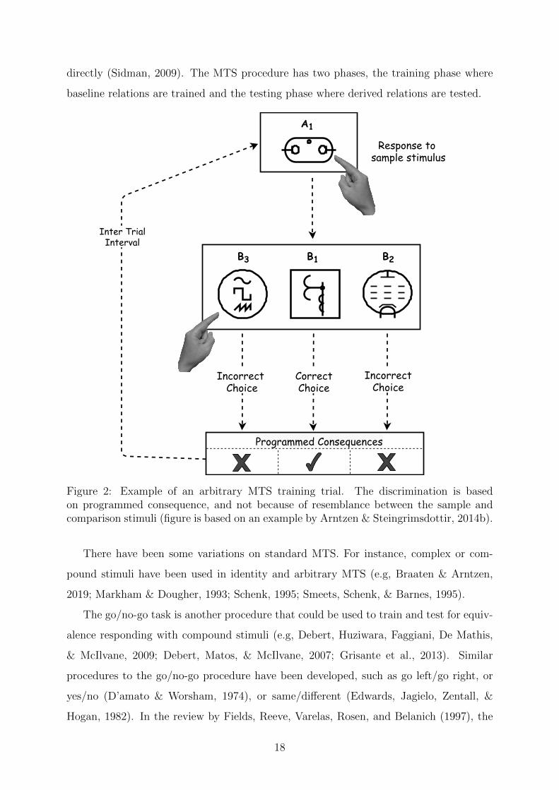
Training structures (training directionality)
In equivalence literature, with MTS procedure three training structures have been used
in establishing conditional discriminations: linear series (LS), many-to-one (MTO) also
known as comparison-as-node, and one-to-many (OTM), also known as sample-as-node (e.g,
Arntzen, 2012). Figure 3 shows the training structures for three-members equivalence
classes. The order of training relations are: AB, and BC in LS; AC, and BC in MTO;
and AB, AC, in OTM settings. There are several studies on the differences between LS,
OTM, and MTO training structures (e.g, Arntzen, 2012; Arntzen, Grondahl, & Eilifsen,
2010; Arntzen & Hansen, 2011).
A B C
A
A
Linear Series (LS)
B
Many-to-One (MTO)Comparison-as-node
One-to-Many (OTM)Sample-as-node
B
C
C
Training Structures
Figure 3: Training structures for an equivalence class with three members indicating by A,B, and C letters. Solid arrows show the training relations and dashed lines show derivedrelations, or test relations. Training relations are: AB, and BC in LS; AC, and BC inMTO; and AB, AC, in OTM (e.g, Arntzen, 2012).
Class Size vs. Number of Classes
Class size refers to the number of members within a class. Class size and number of
classes may also affect the formation of stimulus equivalence classes. For instance, the
19

reported results of two experiments that have been conducted to study stimulus equiva-
lence as a function of class size and number of classes indicate that the number of nodes
disrupts the probability of equivalence class formation more significantly than the number
of classes (Arntzen & Holth, 2000).
Nodal Number
A node in equivalence class terms refers to any stimulus, or class member, which is
related to at least two other members in the equivalence class through training. Stimuli
that relate to only one other stimulus in a class are referred as singles (Fields & Verhave,
1987). Nodal number (Sidman, 1994) or nodal distance (Fields & Verhave, 1987) is the
number of nodes between two members of the equivalence class. Nodal number specifies
the smallest number of required baseline nodes for particular new stimulus pairs to become
members of a relation. For instance, when AB and BC relations are trained, the nodal
number for AC relation is one (see linear series in Figure 3). Nodal density refers to the
number of stimuli related to a particular node. In the AB/BC training, the nodal density
of B is two for AC/BC training, the nodal density of C is two and for AB/AC the nodal
density of A is two, see Figure 3.
Relatedness in Equivalence Class
In stimulus equivalence literature, it has been postulated that after the baseline relations
are trained well in typical humans, all the stimuli in an equivalence class are each equally
related to each other (e.g, Barnes, Browne, Smeets, & Roche, 1995; Fields, Adams, Ver-
have, & Newman, 1993; Sidman & Tailby, 1982). However, evidence from experimental
studies show that under some conditions, different stimuli can have different levels of
relatedness (see, Doran & Fields, 2012, for more details). Fields and Verhave (1987) ad-
dress the effect of class size, number of nodes, training directionality, and nodal density,
either alone or in conjunction with each other, on the relatedness between stimuli in an
equivalence class. The study by Spencer and Chase (1996) addresses the relatedness on
equivalence formation by measuring the response speed during equivalence responding
and provides a temporal analysis of the responses. A decrease in the relatedness between
the members with higher nodal number is observed too in Fields and Verhave (1987).
Likewise, Doran and Fields (2012) show that stimuli within an equivalence class are dif-
20
ferently related based on nodal distance and relational type. The degree of relatedness
between equivalent stimuli has been studied using more sensitive measures than MTS
results (e.g., Bortoloti & de Rose, 2011) confirming the notion that equivalent stimuli
may differ in their degree of relatedness.
Delayed Matching-to-Sample
Conditional discriminations procedures might be either simultaneous MTS or delayed
MTS (see, Arntzen, 2006, as the first parametric study combining delayed MTS and
equivalence performance). In simultaneous MTS, the sample stimulus is presented along
with the comparison stimuli, however, in delayed MTS, the sample stimulus appears first
and disappears for some programmed time before the comparison stimuli are presented.
Simultaneous MTS procedures are applicable when studying learning, while delayed MTS
procedure is relevant for the study of memory (Blough, 1959; Palmer, 1991). The delay
period could be fixed or could be “titrating”. Titrated delayed MTS method, also referred
to as adjusting delayed MTS (Cumming & Berryman, 1965; Sidman, 2013), changes the
length of the delay as a function of the participants’ responses using trials and errors.
In this sense, the participants’ responses provide additional information about the re-
membering behavior of the participant. Titrated delayed MTS has been used to study
remembering in a variety of settings, including to study important variables in analyzing
short-term memory problems (e.g, Arntzen & Steingrimsdottir, 2014a). Delayed MTS
procedures often increase the equivalence responding yield, which could be the result
of rehearsal to keep the sample information during the delay until comparison stimuli
appear (e.g, Arntzen & Vie, 2013).
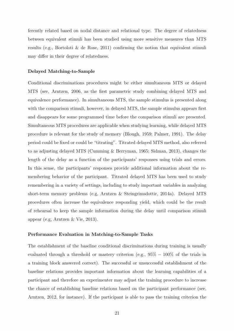
Performance Evaluation in Matching-to-Sample Tasks
The establishment of the baseline conditional discriminations during training is usually
evaluated through a threshold or mastery criterion (e.g., 95% − 100% of the trials in
a training block answered correct). The successful or unsuccessful establishment of the
baseline relations provides important information about the learning capabilities of a
participant and therefore an experimenter may adjust the training procedure to increase
the chance of establishing baseline relations based on the participant performance (see,
Arntzen, 2012, for instance). If the participant is able to pass the training criterion the
21

derived relations will be tested. Usually the criterion ratio in the test phase is lower
than its equivalent in the training phase and there is no programmed consequence. By
passing the criterion for testing in all relations, the equivalence class is considered to be
formed (Sidman & Tailby, 1982).
Reaction time (Dymond & Rehfeldt, 2001; Whelan, 2008) or speed (Imam, 2006;
Spencer & Chase, 1996) can be considered as a supplementary measure worth analyzing in
the stimulus equivalence research. The research on reaction time shows that the response
latency for symmetry trials is longer compared to the baseline relations and even longer
in transitivity and equivalence trials, moreover, reaction time toward the end of testing
is lower compared to the beginning ( e.g., Bentall et al., 1993; Holth & Arntzen, 2000).
Moreover, the stimulus equivalence literature has been expanded by using additional
measures, including sorting tests (Arntzen, Granmo, & Fields, 2017), brain imaging such
as fMRI (Dickins, 2005; Dickins et al., 2001) and EEG recording (Arntzen & Steingrims-
dottir, 2017; Haimson, Wilkinson, Rosenquist, Ouimet, & McIlvane, 2009), or eye-tracking
analysis (Dube et al., 1999; Hansen & Arntzen, 2018; Steingrimsdottir & Arntzen, 2016).
These additional measures could lead to fine-grained analysis of the conditional discrimi-
nations learning and stimulus equivalence responding (Palmer, 2010).
Adaptive Behavior and Learning
Time delay procedure, first was used by Touchette (1971) in teaching discrete responses to
individuals with intellectual disability. From then, time delay and its modifications have
been used in the fields of special education, speech-language pathology, and early inter-
vention (Pennington, 2018). As it has been mentioned, delayed MTS and titrated delayed
MTS can be used as measurement techniques in short-term memory studies (Arntzen &
Steingrimsdottir, 2014a; Sidman, 2013). Spaced Retrieval Training (e.g., Camp et al.,
1996; Camp et al., 1989) is another method of learning and retaining target information
by recalling the information over longer intervals. These methods can be seen as instances
of adaptive learning and the delay time can be addressed by applying theories from the
psychometrics field. In the following, a brief overview of the research from behavior anal-
ysis scientists in education and adaptive learning is provided. The field of psychometrics
and its use in personalized learning is also addressed in this part.
22

Behavior Analysis in Education
The history of applying behavior analysis theory in the design and production of hardware
and apparatus as well as methods and practices is quite rich (Twyman, 2014). Skinner’s
Technology of teaching, published in 1968, reflects his theoretical perspective applied
to problems in teaching and learning (Skinner, 2016). To surpass the usual classroom
experience, Skinner designed and implemented a series of studies to improve teaching
methods for spelling, math, and other school subjects using a teaching machine (Skinner,
1954, 1960). A teaching machine could be any device which arranges contingencies of
reinforcement. The teaching machine of Skinner was a mechanical device that uses an
algorithm which combines teaching and testing items and helps the student to gradually
learn the material via a sort of reinforcement learning. Skinner teaching machine aims
to provide a problem tailored precisely to a student skill level, not to the class average,
and assesses every answer immediately to determine the next learning step. Tailored
or personalized learning can not usually achieved in nowadays learning classes given the
scarcity and cost of human teachers, which motivates using a teaching machine to handle
this type of tailored learning.
Keller formulated the Personalized System of Instruction for college teaching (Keller,
1968). Personalized System of Instruction is a widely used teaching plan composed of
small, self-paced, modularized units of instruction with guidance to lead learners over the
modules until they achieve mastery (see, Twyman, 2014, for more details on how behavior
analysis has contributed to the field of education). It is noteworthy that the importance of
tailoring stimuli in learning has also been studied through stimulus equivalence method-
ology (Arntzen & Eilertsen, 2020).
Mathematical Psychology and Psychometrics
A model, which is central in scientific research, can be seen as a simplified illustration of
a system to reduce its complexity and its behavior quantitatively and also qualitatively.
Model types can be conceptual, verbal, diagrammatic, physical, or formal (mathematical).
The central function of modeling is to turn vague and complex ideas into accessible,
explicit, and precise enough so that their implications become clear (e.g, McClelland,
1988).
Devising models mimicking the brain mechanisms is quite hard in psychological science
23

due to the brain’s incredible complexity. Busemeyer et al. (2015) address the benefits of
modeling in this complex area as follows:
Nonetheless, the resources of mathematical modeling, neuroscientific knowl-
edge and techniques, and excellent behavioral and neuropsychological exper-
imental designs offer the best we can hope for. ...Electrical engineering and
computer science have long possessed rigorous quantitative bodies of knowl-
edge; we could call them meta-theories, of how to infer the internal mechanisms
and dynamics from observable behavior. (Busemeyer et al., 2015, p. 91).
Historically, the application of mathematics to psychology dates back to at least the
seventeenth century (Batchelder, 2015); theories for experimental phenomena led to the
field of mathematical psychology in the 1950s and statistical methods for measuring in-
dividual differences led to the field of psychometrics in the 1930s. Since experimental
psychology was dominated by behavioral learning theory in 1950s, mathematical mod-
els of the learning process (or mathematical learning theory) became a central topic in
mathematical psychology (Bush & Estes, 1959).
Psychometrics is rather concerned more with how psychological constructs, such as
intelligence, neuroticism, or depression, can be optimally related to observables, like out-
comes of psychological tests, genetic profiles, and neuroscientific information (e.g, Bors-
boom, Molenaar, et al., 2015). The psychometric model, in a sense is a measurement
model that integrates the correspondence between observational and theoretical terms.
The measurement model falls under the scope of item response theory (IRT), a subfield
of psychometrics, if the observed variables are responses to test items. IRT can be seen
as a collection of measurement models which is especially important in the analysis of
educational tests and adaptive testing (e.g, Chen & Chang, 2018).
Briefly, IRT offers several advantages over classical test theory: (1) it pro-
vides more in-depth insight at the item level; (2) it facilitates the develop-
ment of shorter measures (by applying computerized adaptive routines); (3)
it detects cross-group variations in item performance (called differential item
functioning or DIF); (4) and it permits linking scores from one measure to
another (Krabbe, 2016, Chapter 10, p. 171).
In IRT-based models, items have different difficulty levels. Defining or measuring task
difficulty can be addressed in many ways. IRT models determine the probability of a
24

discrete result, such as a correct response to an item, based on both item and respondee
parameters using mathematical functions (Krabbe, 2016, Chapter 10).
Adaptive testing has become increasingly important with the advent of computerized
test administration tools. Adaptive testing shortened the test without affecting reliability
by administering items based on the previous item responses of the learner. Computerized
adaptive testing (CAT), also called tailored testing, is a form of computer-based test that
adapts to the examinee’s ability level (e.g, Linden & Glas, 2000). It can be seen as a
form of computer-administered test in which the next item selected to be administered
depends on the correctness of the examinee’s responses to the late items administered (see,
Embretson, 1992, for some contributions of CAT to psychological research).
Adaptive learning designs could also benefit from psychometrics approaches such as
IRT to extract required information for adaptive and personalized learning (Chen, Li, Liu,
& Ying, 2018). An adaptive learning system provides instruction based on the current
status of a learner and together with advances in technology, provides learners with high-
quality and low cost instructions. A recommendation system is a key component of an
adaptive learning system that recommends the next item (video lectures, practices, and
so on) based on the history of learner (e.g, Chen et al., 2018, for some psychometrics ap-
plications in adaptive personalized learning). Adaptive learning in the form of Intelligent
Tutoring Systems, that benefits from the application of artificial intelligence techniques,
will be presented later.
Artificial Intelligence - Machine Learning
Artificial intelligence (AI) is the field devoted to build intelligence demonstrated in ma-
chines, unlike the natural intelligence displayed by humans and animals. Concerning
the concept of intelligence makes AI similar to philosophy and psychology, however, AI
attempts to build artificial intelligent entities in addition to understanding natural intel-
ligence found in nature.
The concept of intelligence has methodically been studied for long times. Scholars
from philosophy and psychology have always attempted to study cognitive functions such
as vision, learning, remembering, and reasoning theoretically and through real experi-
ments. During 1950s, the advent of computer systems led to a paradigm shift as the
25

abstracts contemplation on those cognitive categories to be shaped as real experimental
and theoretical discipline. At the moment, AI is a flourishing field which includes many
sub-fields; from perception and logical reasoning, playing games such as chess and go, to
diagnosing diseases. Due to the increasing popularity of AI, experts in different research
disciplines are getting more interested in AI literature and its applications in their re-
spective research fields. It can also be asserted that AI researchers, who are computer
scientists by definition, have applied AI methodologies to other disciplines and that inter-
disciplinary AI research is gaining a lot of momentum. Therefore, this is fair to claim that
the AI as a field of study has expanded with a broad workability (e.g, Russell & Norvig,
2009, for more details).
Systems that think like humans Systems that think rationally
Systems that act like humans Systems that act rationally
``Theexcitingnewefforttomake computersthink... machineswithminds,inthefullandliteralsense''(Haugeland,1985)
``Theautomationofactivitiesthatweassociatewithhumanthinking,activitiessuchasdecision-making,problemsolving,learning...'' (Bellman,1978)
``Thestudyofmentalfacultiesthroughtheuseofcomputationalmodels''(CharniakandMcDermott,1985)
``Thestudyofthecomputationsthatmakeitpossibletoperceive,reason,andact''(Winston,1992)
``Theartofcreatingmachinesthatperformfunctionsthatrequireintelligencewhenperformedbypeople''(Kurzweil,1990)
``Thestudyofhowtomakecomputersdothingsatwhich,atthemoment,peoplearebetter''(RichandKnight,1991)
``Afieldofstudythatseekstoexplainandemulateintelligentbehaviorintermsofcomputationalprocesses''(Schalkoff,1990)
``Thebranchofcomputersciencethatisconcernedwiththeautomationofintelligentbehavior''(LugerandStubblefield,1993)
Figure 4: Some definitions of AI, based on the categorization by Russell and Norvig (2009,Chapter 1)
Some definitions of artificial intelligence that are collected by Russell and Norvig
26

(2009) are reported in Figure 4. Based on these definitions, an AI researcher might
concerned with either thinking or behavior and want to model humans, or an ideal concept
of intelligence (called rationality). The distinction between a human-centered approach
and a rationalist approach comes from the fact that humans often make mistakes (see,
Kahneman, Slovic, Slovic, & Tversky, 1982, for some of the systematic errors in human
reasoning). Therefore, a human-based approach can be seen as an empirical science,
involving hypothesis and experimental confirmation, while a rationalist approach involves
a combination of mathematics and engineering (Russell & Norvig, 2009). Regardless of
which approach is chosen to the AI, better understanding of brain and intelligent behaviors
in humans and animals could play an essential role in building intelligent machines (see,
Hassabis, Kumaran, Summerfield, & Botvinick, 2017, for some advances in AI that have
been inspired from neuroscience).
In the following, first some artificial neural network models, known as connectionist
models are briefly introduced. Then, reinforcement learning models and some specific
types that are more relevant to this thesis are reviewed.
Neural Networks and Connectionist Models of Cognition
A Computational model, typically studies a complex system by running a simulation on
a computer with the desired parameters and interpreting the behavior of the model. The
computational models in the field of cognitive science are referred to as computational
cognitive models or computational psychology which can be theories of cognition; mostly
process based theories (e.g, Sun, 2008).
Historically, the first known artificial unit based on biological neurons is the McCulloch-
Pitts neuron (McCulloch & Pitts, 1943) which is an abstracted version of a real neuron and
functions as a logic gate, which is assumed to be the main function of a neuron. These
types of neurons are also known as threshold logic units (e.g, Kruse, Borgelt, Braune,
Mostaghim, & Steinbrecher, 2016) since a symbolic logic is applied in order to describe
what neural nets can do. In McCulloch-Pitts nets, a neuron becomes active and sends a
signal to other neurons if it receives enough excitatory input that is not compensated by
equally strong inhibitory input.
Perceptron (Rosenblatt, 1958) is one of the first major advances from the McCulloch-
Pitts neuron with the ability to classify some pattern of input data. Perceptron uses
27

non-binary input and weight connections, and adjust the weights so that network can
learn. In such models an artificial neuron is not equivalent to a single biological neuron,
but rather a population of neurons performing a particular function. Some of Rosenblatt’s
predictions for future of perceptrons demonstrated to be surprisingly accurate:
Later Perceptrons will be able to recognize people and call out their names
and instantly translate speech in one language to speech or writing in another
language, it was predicted.2
The idea of using changes in the weight values of the network for learning in artificial
neural networks is based on the biological neural systems and a simple rule of synaptic
plasticity which is proposed by Hebb (1949):
When an axon of cell A is near enough to excite a cell B and repeatedly or
persistently takes part in firing it, some growth process or metabolic change
takes place in one or both cells such that A’s efficiency, as one of the cells
firing B, is increased. p.62, Hebb (1949)
This type of learning, known as Hebb’s rule or associative learning, suggested that connec-
tions between neurons with correlated activity must be strengthened; a postulate which
is supported by a large body of experimental evidence (see Karaminis & Thomas, 2012;
Sommer, 2012).
Adding hidden layers to perceptrons yields multi-layer perceptrons, which are basically
the Feedforward neural networks, known also as parallel distributed processing (PDP)
models, Connectionist models, and deep learning. Feedforward networks are called so
since the signals pass along only one way; forward (see Figure 5 for the general struc-
ture of feedforward neural networks). Although Feedforward neural networks are not
considered as biologically plausible, these networks can be seen as universal function ap-
proximation where many applications of the AI is based on these types of networks; such
as object recognition tasks, speech recognition, image processing, self-driving cars (see,
Liu et al., 2017, for a survey of on architectures and applications of such networks).
The Backpropagation algorithm which was introduced in the 1970s, became an impor-
tant fast learning approach to neural networks after famous paper by Rumelhart, Hinton,
and Williams (1985). Feedforward neural networks uses backpropagation algorithm in
2The New York Times, “New Navy Device Learns By Doing” (8 July 1958)
28

training for supervised learning and this algorithm is the workhorse of learning in neural
networks. Briefly, the network processes the input and by passing signals through layers
produces an output. Since the learning is supervised, the correct output is known and
therefore the error can be calculated. The network has to figure out how to change the
weights (learning is through adjusting the weights) in order to generate outputs closer to
the right answer. This weight adjustment is for all the connections in the network and
network must figure out how much of the error is due to a particular connection and its
weight; this is also known as Credit Assignment Problem (e.g, Schmidhuber, 2015).
Backpropagation algorithm propagates the error backward toward the network and
captures the amount of error due to each connection in order to adjust the weights to
most efficiently decrease the the errors see, LeCun, Touresky, Hinton, and Sejnowski, 1988,
for a theoretical framework of backpropagation algorithm. Convolutional neural networks,
which is highly praised models in neural networks, is categorized as a feedforward neural
network (Krizhevsky, Sutskever, & Hinton, 2012).
Recurrent neural networks is a more biologically plausible model, in comparison with
feedforward nets, which is appropriate to the time-dependent information processing such
as memory, sequences and dynamics. In recurrent neural networks, units are not just
connected and send signals to the forward layer, but they can project into units in the
same layer and the previous layer. Unlike feedforward neural networks where the output
is only a function of input (a static function is computed), in recurrent neural network
the output is a function of input and internal states or history of learning (a dynamic
function is computed). Sometimes it is hard to distinguish and analyze recurrent neural
networks as multi-layer network due to the cycles in the structure which provides the sys-
tem memory. Hopfield neural networks (Hopfield, 1982) which is also known as content
addressable memories is one of the first models of the learning and retrieval of memories
in the brain. Hopfield neural networks could form a full memory using partial informa-
tion related to that memory. The learning in Hopfield is based on Hebb’s rule and the
so-called one-shot learning, where the network needs to observe each query and memory
only once to learn the association between them (Hopfield, 1982). Boltzmann Machine,
also called stochastic Hopfield network with hidden units, is a similar but more powerful
recurrent neural network where units are stochastic (Ackley, Hinton, & Sejnowski, 1985).
Recurrent neural networks appeared in many applications such as natural language pro-
29

cessing (e.g, Collobert et al., 2011), language understanding machine translation, video
processing, music composition and financial markets (Medsker & Jain, 1999). Training
recurrent neural networks is much more challenging than feedforward networks. Back-
propagation through time is a popular solution Which basically transforms a recurrent
network into a feedforward network and update the training weights (Lillicrap & Santoro,
2019). Long Short Term Memory (LSTM) networks is a widely used recurrent neural
network (Hochreiter & Schmidhuber, 1997) which uses memory cells, that is basically a
series of gates. LSTMs’ memory ability make it the standard recurrent neural network in
AI.
Spiking neural networks is another class of neural networks which is a closer model to
the brain, since a real neural network uses spikes, but adding more realism to the model
adds more challenge to train and implement the model.
Both feedforward and recurrent networks use continuous activation functions and back-
propagation which depends on this continues function. In other words, the activity of a
unit can take any value in a range and that value passes through all the connections.
However, real neurons send action potentials, i.e. the neuron send either the spike or
nothing. Spiking neural networks are good models to study how brain works and there is
significant research attention around these networks as an inspiration to the algorithms
in AI (see, Taherkhani et al., 2020, for a review on learning in spiking neural networks).
From cognitive psychology point of view, connectionist models attempt to explain
and replicate intellectual abilities by assuming that neural systems pass activation among
simple, interconnected processing units (McClelland, Rumelhart, Group, et al., 1987).
Connectionist models, or neural network models, are the most commonly used cognitive
model today which similar to all cognitive models, need some building blocks and some
organization for them. The primitives in PDP or connectionist models are units and
connections; with emphasis on the parallel nature of neural processing, and the distributed
nature of neural representation. To define the architecture of a connectionist model,
one decides on the number of units, connectivity pattern between the units, and the
interactions with the environment. The network term typically refers to the set of units
and their connections (McClelland, 1988).
Although Connectionist models have been primarily studied in cognitive science and
cognitive psychology, they have been also applied in behavior analysis studies (Barnes &
30

Input
Hidden
Output
FeedforwardNeuralNetwork
Input
Hidden
Output
RecurrentNeuralNetwork
Figure 5: The general structure of two basic neural networks; feedforward and recurrentneural networks. Deep neural networks usually have many hidden layers. In the learningprocess, the knowledge is stored in the connections by changing the connection weightswhich justifies the connectionism name for these models.
Hampson, 1993; Barnes & Holmes, 1991; Fodor & Pylyshyn, 1988; Staddon & Bueno,
1991).
Computational Reinforcement Learning
Reinforcement learning (RL) refers to the scientific study of how animals, humans, and
machines use the experience to adapt their behavior in order to maximize the received
total reward from an environment (Busemeyer et al., 2015, Chapter 5).
RL is a highly interdisciplinary field of research that lies at the intersection between
computer science, machine learning, psychology, and neuroscience. RL deals with learning
from evaluative feedback (see Figure 6 for a schematic view) and not corrective feedback
bearing similarities to supervised learning which is dominant in the field of machine learn-
ing (Sutton & Barto, 2018). In supervised learning, an external supervisor provides a set
of labeled samples and the objective is to generalize or extrapolate the kind of responses
that are taught during training. Supervised learning, unlike reinforcement learning, is an
inadequate choice for reactive learning from interaction with the environment (see, Sutton
& Barto, 2018, for details of reinforcement learning schemes).
31

Reward
Environment
Agent
Action
State
Figure 6: The general structure of an RL interacting with environment. At each timestep, the agent perceives the state of environment, performs an action and receives afeedback. The feedback is the source of learning for the agent which tries to revise itsfuture actions to maximize its total received reward over time.
Projective Simulation
A newly developed particular type of RL agent, called Projective Simulation (PS) agents (Briegel
& De las Cuevas, 2012) is presented in this section (for detailed comparisons of RL and
PS, see Bjerland, 2015; Mautner, Makmal, Manzano, Tiersch, & Briegel, 2015).
PS model, similar to other reinforcement learning algorithms, can be embodied in
an environment, to perceive stimuli, execute actions, and learn through trial and error.
The PS episodic memory is perhaps the most important difference of PS with other
standard RL algorithms which facilitates modeling more complex features. Learning in
standard RL algorithms is based on estimation of value functions, whilst in PS learning
is through the re-configuration of episodic memory. This re-configuration could be either
by updating transition probabilities or by adding/creating new clips (Bjerland, 2015;
Melnikov, Makmal, Dunjko, & Briegel, 2017).
PS agent interaction with the environment is similar to other RL agents, so that the
agent receives a precept, chooses an action among the possible actions which usually leads
to a reward (positive or negative) from environment. Note that usually negative reward
is referred to as penalty. The agent then tries to bias its actions towards the actions
with positive rewards. The internal mechanism of PS by which agents act is based on a
directed, weighted network of clips, so called Episodic and Compositional Memory (ECM),
32

where each clip could represent a remembered percept, action, or sequences of them. It
is noteworthy that the term episodic memory has been coined by Tulving et al. (1972) to
refer to the ability to vividly remember specific episodes of one’s life. EMC memory in PS
agents can be described as a probabilistic network of clips (see Figure 7 for a schematic
view of a network clip in PS agents).
!"#$"!%
$&$'
$( $)
!(,'
!(,)
$+
$,
$-
$.
$/
!',,
!',-
!),+
!),-
!.,&
!/,&
0$%123
$4!),4!-,4
!',+
Figure 7: A memory network in PS model and a random walk on the clip space whichstarts with activation of clip cs and reaches the action clip ca that coupled-out the realaction. The clips and transition probabilities between them can evolve based on theenvironment feedback.
As demonstrated in Figure 7, once a percept is observed by agent, a clip corresponding
to the percept is activated and a random walk on the clip network triggers. When an
action clip is reached, agent realises the corresponding action. The probabilities of going
from one clip to the next are based on the connection weights of the relevant edges, so
called h-value. If agent receives reward for the chosen action, the edges traversed to reach
that decision are reinforced and as a result the probability of repeating the same behavior
will be increased. The learning in PS agents is not limited to updating the connection
weights through Bayesian rules. The structure of network clip can also be altered by
creating and adding new clips. New clips, can be added either by composing existing ones
under certain compositional principles, or by adding blank clips that can represent novel
content (Melnikov et al., 2017).
Stochastic Point Location (SPL)
Stochastic Point Location (SPL) problem, also synonymously known as Stochastic Search
on the Line (SSL), deals with searching for an unknown point in an interval under faulty
33
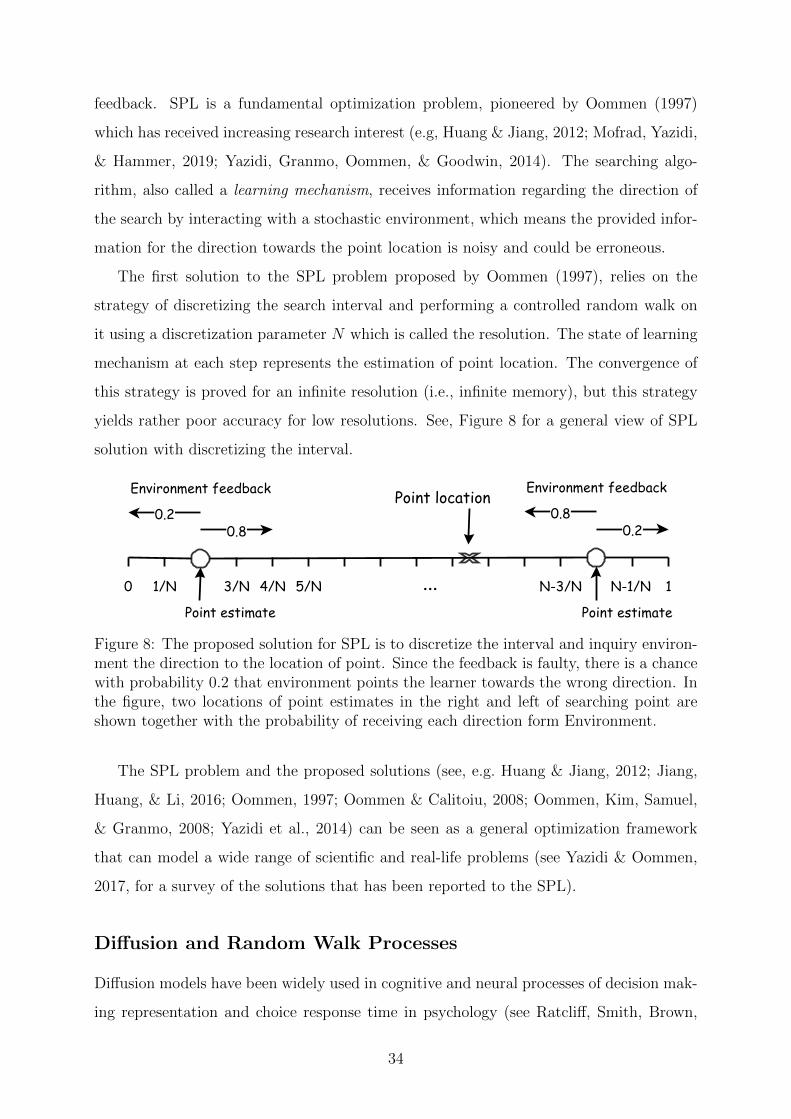
feedback. SPL is a fundamental optimization problem, pioneered by Oommen (1997)
which has received increasing research interest (e.g, Huang & Jiang, 2012; Mofrad, Yazidi,
& Hammer, 2019; Yazidi, Granmo, Oommen, & Goodwin, 2014). The searching algo-
rithm, also called a learning mechanism, receives information regarding the direction of
the search by interacting with a stochastic environment, which means the provided infor-
mation for the direction towards the point location is noisy and could be erroneous.
The first solution to the SPL problem proposed by Oommen (1997), relies on the
strategy of discretizing the search interval and performing a controlled random walk on
it using a discretization parameter N which is called the resolution. The state of learning
mechanism at each step represents the estimation of point location. The convergence of
this strategy is proved for an infinite resolution (i.e., infinite memory), but this strategy
yields rather poor accuracy for low resolutions. See, Figure 8 for a general view of SPL
solution with discretizing the interval.
0 1/N 3/N 1N-1/N...4/N
Pointlocation
0.80.2
Environmentfeedback
Pointestimate
5/N N-3/N
Pointestimate
0.20.8
Environmentfeedback
Figure 8: The proposed solution for SPL is to discretize the interval and inquiry environ-ment the direction to the location of point. Since the feedback is faulty, there is a chancewith probability 0.2 that environment points the learner towards the wrong direction. Inthe figure, two locations of point estimates in the right and left of searching point areshown together with the probability of receiving each direction form Environment.
The SPL problem and the proposed solutions (see, e.g. Huang & Jiang, 2012; Jiang,
Huang, & Li, 2016; Oommen, 1997; Oommen & Calitoiu, 2008; Oommen, Kim, Samuel,
& Granmo, 2008; Yazidi et al., 2014) can be seen as a general optimization framework
that can model a wide range of scientific and real-life problems (see Yazidi & Oommen,
2017, for a survey of the solutions that has been reported to the SPL).
Diffusion and Random Walk Processes
Diffusion models have been widely used in cognitive and neural processes of decision mak-
ing representation and choice response time in psychology (see Ratcliff, Smith, Brown,
34

& McKoon, 2016, for a survey of diffusion models in psychology). Decision making in
diffusion models are based on accumulating samples of noisy evidence to a response crite-
rion, where new information is used to update beliefs and choose future actions. Decision
making is considered as a statistical process, where successive samples of noisy evidence
or stimulus information are accumulated until a response criterion is meet. The noisy
evidence assumption comes from either the fact that the stimulus itself is composed of a
sequence of noisy events or from the noisy coding in the neural system. Random walk
models can be seen as the discrete-time counterpart of diffusion models (Smith & Ratcliff,
2015).
Network enhancement is based on (Zhou, Bousquet, Lal, Weston, & Scholkopf, 2004)
to solve semi-supervised labeling problem where some of the data points are labels where
the majority was unlabeled. A diffusion process is used to label the rest of the data points
by diffusion of information globally over local graph structure in an iterative manner.
In semi-supervised learning problems the prior assumption of consistency is essential,
that is nearby units most probably have the same label and units on the same structure
are expected to have the same label. The former assumption is local, and the latter
assumption is global.
As Zhou et al. (2004) explicitly mention, the Network enhancement is inspired by
“spreading activation network” in experimental psychology.
This algorithm can be understood intuitively in terms of spreading activation
networks (Anderson, 1983; Shrager, Hogg, & Huberman, 1987) from experi-
mental psychology.
Spreading activation refers to a class of algorithms that propagate activation levels
in a network in order to select the most closely related nodes to the activation source.
The idea of tracing chains of connections addressed in experimental psychology research,
and in the theories of psychologists such as Freud and Pavlov (Anderson, 1983). Quillian
(1967) introduced spreading activation as a computational process that can accomplish
search in semantic networks. Collins and Loftus (1975) proposed a version of the semantic
network model which activation values simultaneously spread through all network links
to account for semantic priming phenomena. In psychological models spreading activa-
tion is used for selecting among several possible related memories or actions when the
situation is ambiguous (Shrager et al., 1987). Zhou et al. (2004) algorithm which is in-
35

spired by spreading activation networks (Shrager et al., 1987) updates, let every unit in
the network iteratively spread its label information to its neighbors until a global stable
state is achieved. The algorithm controls the relative amount of the information from
unit neighbors and its initial label information using a regularization parameter. Network
Enhancement model (Wang et al., 2018) introduced an iterative algorithm for denoising
weighted networks with inspiration from the local and global consistency proposed by
Zhou et al. (2004). Specifically, Wang et al. (2018) introduced a localized network to cap-
ture the information of all paths of length three or less connecting any given two nodes
which is used for spreading the information and updating the network weights.
Applications of Network Enhancement Network Enhancement has found mul-
tiple applications which include enforcing similarity links between individual based on
genomics data (Wang et al., 2014), image segmentation in computer vision (Wang, Jiang,
Wang, Zhou, & Tu, 2012), community detection (Hu, Wang, Chen, & Dai, 2020).
Network Enhancement
Network Enhancement (NE) (Wang et al., 2018) is a diffusion-based computational ap-
proach that has been proposed for denoising weighted biological networks. NE converts a
noisy, undirected, weighted network into a network with the same nodes but different con-
nections and weights. The basic assumption is that nodes which are connected through
paths with high weight edges, most probably are directly connected with a high weight
edge. In this regards, the diffusion process in NE uses random walks of length three or
less and a regularized interaction flow in order to revise edge weights (See Figure 9 for an
illustration).
The NE algorithm, takes as an input a weighted network, and iteratively updates its
associated weighted adjacency matrix using the NE diffusion process. NE can be used for
a more accurate detection of modules/clusters in the network.
Related Works
In this section the existing computational models of equivalence classes in behavior anal-
ysis domain as well as Intelligent Tutoring Systems as adaptive learning models are re-
viewed.
36

nodeA
nodeB high-interactionflow node
AnodeB low-interactionflow
Figure 9: Network enhancement updates the network structure by updating the connec-tion weights based on the neighboring connections and paths of length two and three. Inthe left panel, there are strong paths between node A and node B and therefore, networkenhancement increases the direct connection weight between them. The opposite scenariois in the right panel, where due to the low-weight connections network enhancement pro-cess decreases the weight of direct connection. This figure is a modification of proposedillustration by Wang et al. (2018).
Computational Models of Equivalence Classes
Artificial neural networks could advance the understanding of way derived stimulus re-
lations are formed, by either simulating MTS procedures (Barnes & Hampson, 1993;
Cullinan, Barnes, Hampson, & Lyddy, 1994; Lyddy, Barnes-Holmes, & Hampson, 2001;
Tovar & Westermann, 2017) or training stimulus relations through compound stimuli and
alternative procedures to MTS (Tovar & Chavez, 2012; Vernucio & Debert, 2016).
A well-known behavior-analytic approach to modelling with neural networks is the
network for relational responding, called RELNET (Barnes & Hampson, 1993) which was
designed to simulate complex human behaviors, from the RFT perspective. The model
is a feed-forward neural network that uses standard backward-error propagation (Rumel-
hart et al., 1985) for learning. Three modular stages of RELNET are an encoder that
preprocesses the stimuli for the relational responding machine (central system) as the
second stage, and the third stage is a decoder that decodes the output of the central
system. The simulation of learning task is performed through the central system and the
encoder and decoder act like a simple pattern association. Barnes and Hampson (1993)
replicated the empirical study by Steele and Hayes (1991) which is a contextual control
of derived stimulus relations with MTS procedure. Modified versions of RELNET have
been used to simulate other examples of derived relational responding (see, e.g. Cullinan
et al., 1994). RELNET is also used to study the effect of training protocols in equiva-
37

lence class formation (Lyddy & Barnes-Holmes, 2007) through modeling the experiment
by Arntzen and Holth (1997). However, Barnes and Hampson (1997) discuss that lack of
neural plausibility is the major weaknesses of RELNET model. Tovar and Chavez (2012),
also criticise the RELNET model by arguing that the transitive relations are partially
trained during encoding which means the model purpose to form untrained relations is
not completely meet.
Another computational model of formation of equivalence classes with MTS procedure
is presented by (Tovar & Westermann, 2017). The proposed fully interconnected neural
network model links stimulus equivalence field to Hebbian learning, associative learning
and categorization. In the model, each neuron accounts for a stimulus represented through
activation. The weighted connections among neurons spread activation in the network,
and coactivation of neurons based on Hebbian learning, updates the connection weights.
Three high impact studies (Devany, Hayes, & Nelson, 1986; Sidman & Tailby, 1982;
Spencer & Chase, 1996) have been simulated with this model. To validate the model,
the connection weights in the neural network were compared with the results of real
experiments.
Tovar and Chavez (2012) used a three-layer feed-forward neural network to train stim-
ulus equivalence relations with compound stimuli procedures. The network inputs are
stimulus pairs (e.g., A1B1, A1B3) and the outputs are yes/no responses. In order to
derive relations in desired classes, this model requires a previous learning of all possi-
ble relations of an equivalence class, say XY Z. Vernucio and Debert (2016) considers a
replication of this model with a go/no-go procedure, i.e. just considering a yes responses.
Although RELNET, yes/no, and go/no-go models successfully replicate the formation
of equivalence classes, they are not addressing relatedness between members of stimulus
classes, and therefore they are not considered to be biologically plausible (O’Reilly &
Munakata, 2000; Tovar & Westermann, 2017).
The real time neural network model presented by Lew and Zanutto (2011) is based on
biological mechanisms that are able to learn different tasks such as operant conditioning
and delayed MTS. The first layer of this three layers network receives sensory input from
the environment and produces short-term memory traces of them. The second layer’s job
is further filtering of task relevant stimuli which will in the third layer be associated with
the proper response (for an application of the model, see Rapanelli, Frick, Fernandez, &
38

Zanutto, 2015).
An overview of existing connectionist models of formation of equivalence relations is
provided by (Ninness, Ninness, Rumph, & Lawson, 2018) along with a neural network
framework called emergent virtual analytics (EVA), where the process of applying neural
network simulations in behavior-analytic research is demonstrated (see Ninness, Rehfeldt,
& Ninness, 2019, for more simulations with EVA).
Computational Theories for Adaptive Testing and Learning
Several studies show that personalized learning is the key to increased fulfillment of po-
tential (e.g, Miliband, 2004). A possible solution to the latter problem is resorting to the
advances in AI in order to personalize the teaching process. Achieving computer tutoring
systems that are as effective as human tutors can be traced back to the earliest days of
computers (Smith & Sherwood, 1976). Recent research indicate that computer tutoring
systems can raise student performance beyond the level of traditional classes and even
beyond the level of students who learn from human tutors see, Kulik and Fletcher, 2016,
for a survey. Chirikov, Semenova, Maloshonok, Bettinger, and Kizilcec (2020) show that
online education platforms could scale high-quality science, technology, engineering, and
mathematics (STEM) education through national online education platforms at universi-
ties. This means that such instruction can produce similar learning outcomes for students
as traditional, in-person classes with a much lower cost see also, VanLehn, 2011, for a
review of relative effectiveness of human tutoring, intelligent tutoring systems, and no
tutoring.
Intelligent Tutoring System (ITS)
Intelligent systems (also known as intelligent tutoring systems), is a broad term and con-
sists of any computer program or educational software containing an artificial-intelligence
component (Freedman, 2000). ITS aims to provide personalized sophisticated instruc-
tional advice which outperforms conventional computer-aided instruction systems which
is comparable with human tutors. ITS can be classified according to their underlying
algorithm. Model-tracing tutor, is a well-known category where the algorithm tracks the
progress of student and controls the performance to be in an acceptable interval by adjust-
ing feedback and providing guidance along the way (e.g, Freedman, 2000; Shute & Zapata-
39

Rivera, 2010). Sleeman and Brown (1982) pioneered the idea behind ITS for designing
systems assisting students reach their full potential in a limited amount of time. There are
different artificial intelligence approaches to create an ITS including multi-armed bandits
(e.g, Clement, Roy, & Oudeyer, 2015), Bayesian-networks (e.g, Millan, Loboda, & Perez-
de-la-Cruz, 2010) and neural-networks (e.g, Zatarain Cabada, Barron Estrada, Gonzalez
Hernandez, & Oramas Bustillos, 2015). Many ITSs are based on Computerized Adap-
tive Testing (CAT) which as mentioned earlier is an efficient computer-based testing (see
for instance Hatzilygeroudis, Koutsojannis, Papavlasopoulos, & Prentzas, 2006; Jansen,
Hofman, Savi, Visser, & van der Maas, 2016; Kozierkiewicz-Hetmanska & Nguyen, 2010).
In adaptive testing, the aim is to estimate the participant’s ability and administration
of problems should provide as much information as possible (Birnbaum, 1968; Eggen &
Verschoor, 2006). Adaptive learning or training, on the other hand needs to consider
other factors which are the motivation and involvement of participant (Jansen et al.,
2016). In most adaptive testing and CATs, selection of problems is due to the partici-
pant’s current estimated ability (see, Eggen & Verschoor, 2006, for instance) which means
when the probability of success equals to 0.5. This condition provides highest information
and minimizes the test length. This level of challenge could be frustrating for many of
participants and trade-off between the length of the test and motivation and pleasure of
students is needed. For instance, by using a higher success rate, CAT principles have been
successfully applied for practicing math skills (e.g, Jansen et al., 2016; Jansen et al., 2013;
Klinkenberg, Straatemeier, & van der Maas, 2011). The optimal strategy for motivating
the student has been investigated by Lumsden (1994) which is backed up by Clement
et al. (2015) where the tasks should be slightly beyond the participant’s current abilities,
concurring with theories of intrinsic motivation.
Despite that research on ITS has produced many interesting theoretical insights, using
ITS regularly in schools is not common and there is more effort that is needed to deploy
ITS in real-life learning settings (Shute & Zapata-Rivera, 2010).
Works on Learning Automata (LA) and ITSs e.g, Oommen and Hashem, 2013 can
be addressed here. In simple terms, LA is a stochastic machine attempting to find the
optimal strategy from a set of actions in a random environment. LA is particularly
important in decision making under uncertainty see, Narendra and Thathachar, 2012, for
an introduction to LA. The term tutorial-like systems refers to study tutorial systems
40

while no entity needs to be a real-life individual. So, all the component of the model
are basically an algorithm that simulate the real teacher, student, knowledge-domain,
etc (Oommen & Hashem, 2013).
For a few design and analysis of tutorial-like system models using LA, consider model-
ing of a student (Oommen & Hashem, 2009b), modeling of a classroom of students where
artificial students can interact and learn from each other as well as the teacher (Oom-
men & Hashem, 2009a), modeling of a (stochastic) teacher (Hashem & Oommen, 2007),
modeling the domain knowledge (Oommen & Hashem, 2010), and modeling how teaching
abilities of a teacher can be improved (Oommen & Hashem, 2013).
Studies Conducted for the Dissertation
The four studies included in this thesis propose computational models of formation of
stimulus equivalence classes and adaptive testing and adaptive learning. A summary of
the papers is provided first, followed by ethical considerations and discussion.
Summary of the Studies
Study I
In this study, formation of stimulus equivalence classes through a MTS procedure has
been modeled based on a reinforcement learning framework called projective simulation
(PS) (Briegel & De las Cuevas, 2012). In order to make the PS model appropriate for
stimulus equivalence, we modify the model and name it, equivalence PS (EPS). To the best
of our knowledge, EPS is the first study which proposes a computational model in stimulus
equivalence based on machine learning. The extra features that EPS has, in comparison
with PS, can be further used in machine learning research. The proposed model is as a
transparent model as opposed to black-box models in AI and is able to control various
factors such as learning rate, forgetting rate, symmetry and transitivity relation formation
and stimulus relatedness through nodal number. The model is able to mimic both typical
participants and participants with some disabilities. The influential experimental studies
in behavior analysis literature due to Sidman and Tailby (1982), Devany et al. (1986),
and Spencer and Chase (1996) have been simulated with our EPS framework in order
to validate our model. Alternatives by which a hypothetical experiment in stimulus
41

equivalence research can be studied through EPS have also been discussed in this study.
The learning algorithm, similar to empirical settings, has two phases, the training phase
where the clip network will be shaped and the testing phase where the clip network is used
to cope with new, derived relations. In the proposed model (EPS) a directed graph is used
to differentiate between all types of relations. The symmetry relations are formed during
training, and we assume transitivity and equivalence relations are also formed during
training. However, transitivity and equivalence transition probabilities are calculated on
demand upon trials in the MTS test, which is based on the findings that the response
latencies in transitivity and equivalence tests are typically longer than trained relations
or symmetry tests (Bentall et al., 1993). We propose several methods to address the
test phase and derived relations, including max-product, memory sharpness, and random
walk on the memory network with absorbing action sets. The transitive and equivalence
relations in EPS model are not a part of clip network and they are derived upon request,
i.e. when they appear in a MTS trial during the testing phase. The formation of symmetry
relations, by virtue of the flexibility of PS, can be postponed until the testing phase. On
the other hand, it is possible to establish all the connections in the training phase and
gradually update them during MTS training phase, or during the MTS test.
Study II
Enhanced EPS (E-EPS) model that builds upon EPS proposed a new way of modeling
derived relations which possesses many advantages in comparison with EPS. The E-EPS
has almost the same training phase as the model in Study I, but derived relations are
formed after training phase using an iterative diffusion process called Network Enhance-
ment (Wang et al., 2018). As a result, in testing phase E-EPS retrieves relations from
memory, unlike EPS where derived relations are computed on demand by using some
type of likelihood reasoning. During the network enhancement phase, the structure of
clip network changes and indirect relations get enhanced.
We can regard the clip network at the end of training phase of EPS as a noisy version of
the agent’s memory network that is supposed to contain all trained and derived relations
strong. Using a denoising approach such as network enhancement could produce a new
less noisy clip network with information regarding the equivalence class formation. We
propose directed NE (DNE) diffusion process by which we can control the formation
42

or non-formation of derived relations. In order to study the role of parameters on the
agent performance in the E-EPS model, various experimental settings are simulated and
discussed. Moreover, training procedures LS, MTO, and OTM are simulated where similar
to the main stream literature in behavior analysis (see, e.g. Arntzen, 2012; Arntzen,
Grondahl, & Eilifsen, 2010; Arntzen & Hansen, 2011), the model yields better performance
in OTM and MTO cases in comparison with LS.
E-EPS has less parameters in comparison with EPS and is a much simpler com-
putational method and yet accurate. Theoretical analysis of the updating process and
convergence guarantees are established.
Study III
The proposed model in this study is a solution to the SPL problem which is a search prob-
lem for a point location in an interval based on the feedback’s from environment. One
of the applications of this model is to find the tolerable difficulty level by the participant
in an adaptive test. To make the model more realistic, the feedback from participants is
assumed to be inaccurate and the workable difficulty level is assumed to be non-stationary
over time. In this study, two major contributions to the SPL problem are proposed. First,
we employ the concept of mutual probability flux between neighboring states along the
line to improve the estimation of the point location. Next, we estimate the error probabil-
ity characterizing the environment while tracking the position of the optimal point. This
study is partially based on our previous work (Mofrad, Yazidi, & Hammer, 2017) by which
we show that the SPL problem can be solved by tracking two multinomially distributed
random variables using the Stochastic Learning Weak Estimator (SLWE) method (Oom-
men & Rueda, 2006). We proposed to integrate the SLWE, which figures among the most
prominent estimators for non-stationary distributions, as the inherent part of a more
sophisticated solution for the SPL. The estimation strategy at each time step revolves
around tracking the distribution and estimating the point location based upon it. Differ-
ent statistical operators namely maximum, expectation, and median have been applied on
the estimated probability vectors to obtain point location estimates. Simulation results
indicate that, the proposed methods produce smoother estimates than those obtained
from other SPL solutions and can track the changes more efficiently. The probability of
receiving correct feedback from environment, called environment effectiveness, is usually
43
unknown and might change over time. As the second contribution of this study, we esti-
mate the feedback error probability in tandem with the unknown location estimation. In
Study III, the participant performance is modeled using a stair function with two levels:
a high performance for difficulties under the optimal “manageable” difficulty level and a
low performance for difficulties just above the same level, i.e., the “manageable” optimal
difficulty level. However, if we rather use a more realistic performance function according
to which the performance is continuous and monotonically decreases as a function of the
difficulty level, the approach in Study III will basically converge to difficulty level for
which the participant performance is at 50% under some mild conditions. Such remark
motivated Study IV in which we resort to the latter realistic performance model, for effi-
ciently finding a higher rates of performance that are motivating enough for the learner,
usually above 50% such as 70%. For a schematic description of approaches to find task
difficulty based on success probability in Study Study III and Study IV see Figure 10.
Study IV
The Balanced Difficulty Task Finder (BDTF) proposed in this study is a method for ad-
equate difficulty task assignment based on the principles adaptive learning. The BDTF
method is general and can be integrated as a part of an ITS system. BDTF has ap-
plications in learning and remembering techniques in behavior analysis methods such as
titrated delayed MTS and online learning environments. The idea behind BDTF is to
select tasks with appropriate difficulty to the learner so that ensure that the level of mo-
tivation and enjoyment during the learning is maintained. The strategy is similar to Elo’s
chess skill rating (Glickman, 1995) and TrueSkill (Herbrich, Minka, & Graepel, 2006) for
matching game players, where players with similar capabilities and skills are matched.
Choosing an appropriate opponent or appropriate game level in BDTF is analogous to
choosing automatically an appropriate level of the learning task. In this regard, each
participant starts with a predefined difficulty level of tasks (Clement et al., 2015), and
based on the performance of the learner the difficulty of future tasks is adjusted in a trial
and error manner.
The difficulty of any given task is mapped to a number between zero and one where
zero denotes the lowest possible difficulty and one denotes the highest possible difficulty.
In BDTF, we assume the chance of success in a given task decreases monotonically as the
44

1 1
0 0
DifficultyLevel DifficultyLevel1
Succ
essprob
ability
Succ
essprob
abilityp
1-p0.5
Succ
essprob
ability
p*
0
DifficultyLevel
1
1
1
p
1-p
d* d*
Decreasingfunction
d*
0.7
0.45
Figure 10: Comparison of Study III and Study IV. The top-left figure represents thestair function with two levels which we used in Study III. p represents high performancefor difficulties under the optimal “manageable” difficulty level d∗, and 1 − p is a lowperformance for difficulties above d∗. The top-right figure, shows the performance ofproposed model if we instead using a more realistic performance function according towhich the performance is continuous and monotonically decreases as a function of thedifficulty level. The approach in Study III will converge to difficulty level for which theparticipant performance is at 0.5 under some mild conditions. The bottom figure, depictsthe approach in Study IV with a more realistic performance model, for efficiently findinga higher rates of performance that are motivating enough for the learner, usually above0.5 such as 0.7.
45
difficulty level increases. The recommended task difficulty gets increased upon success
and decreased upon failure in an asymmetric manner so that we can adjust the difficulty
of the given tasks and consequently drive the system towards a state of flow (Chen, 2007).
Ethical Considerations
Since this work reports no original empirical research, it is not subject to the ethical con-
siderations regarding participants (humans and animals) that psychology research usually
deals with.
On the other hand, ethical concerns regarding AI algorithms appear mostly in the cases
with social dimensions where AI algorithms act as autonomous agents and team-mates.
For instance, avoiding cognitive biases, seeking reliability and applicability in decision-
making domains such as healthcare, and preventing possible harms of AI to humans and
other morally relevant beings (Bostrom & Yudkowsky, 2014).
Computational modelling in basic research though draw different ethical views. Re-
sorting to a modeling approach rather than to an experimental approach, as an alternative
methodology in studies involving human and animal subjects, may allow behavior-analytic
researchers to formulate, explore, and examine ideas prior to full experimental testing.
These models usually are highly controllable and precise and can be promising candidates
for research. Using cognitive and computational models can reduce the possible harm to
the human and nonhuman subjects by limiting the need to test all the ideas on them.
Moreover, in some cases, such as in the case of Relational Frame Theory, that relies on
a long and often complex histories of explicit reinforcement, it would be so difficult, and
even unethical, to test hypothesises directly on subjects in a behavioral laboratory (Barnes
& Hampson, 1997).
An important feature in developing AI algorithms in general and cognitive models in
particular is transparency and interpretability of the models (e.g, Bostrom & Yudkowsky,
2014; Fleischmann & Wallace, 2017). Some modeling paradigms such as neural networks
are not considered practical in many settings even though they yield accurate predictions
as the predictions of those models are opaque and the logic behind them can not be ex-
plained clearly. The area of Explainable Artificial Intelligence (XAI) (see Biran & Cotton,
2017, for a survey on XAI) has been attracting more attention recently due to the need
to increase the trust and transparency of intelligent agents (e.g, Miller, 2019), including
46

the design of models that are inherently interpretable instead of black-box models (see
Rudin, 2019, for instance).
In modeling equivalence formation, it is vital to understand the model and to also
design a biologically plausible model. We found Projective Simulation model as an ap-
propriate candidate for this aim. For adaptive learning, we could apply more complex
models but we rather opted for a fairly simple probabilistic model in favor of interpretabil-
ity and explainability. Therefore, all the proposed models in the studies for this thesis
can be categorized as XAI models with the capability of easy interpretation.
Discussion
The purpose of this dissertation was to propose flexible and interpretable computational
models that replicate formation of stimulus equivalence classes and adaptive learning.
Reinforcement learning agents, in the form of Projective Simulation and Stochastic Point
Location, were the chosen candidates to model the interaction between experimenter and
the participant through the processes.
Although neural networks is one of the most powerful simulation techniques, designing
models that are inherently interpretable instead of black-box models (see Rudin, 2019, for
instance) is an advantage. Projective simulation (Briegel & De las Cuevas, 2012; Mautner
et al., 2015) is a fairly simple graphical model which provides a flexible paradigm that can
be easily extended. Based on projective simulation, we proposed a general simulator for
equivalence relations. In Study I formation of derived relations are computed on demand
through some type of likelihood reasoning. In Study II, Network Enhancement (Wang
et al., 2018) updates the agent memory after training phase and as a result the test
trials become like a memory retrieval phase. The simulators could replicate a variety
of settings in a matching-to-sample procedure. There are different mechanistic accounts
on the formation of stimulus equivalence classes and derived relations. Galizio, Stewart,
et al. (2001) discuss that some degree of equivalence class formation occurs during the
MTS training, which is further enhanced during the testing. In many studies, on the
other hand, the emergence of equivalence relations is considered to be only the result of
testing lower-stage relations (see, part E of Dickins, 2015, for a discussion). Different
approaches to the test phase proposed in Study I and Study II can be interpreted in
accordance with different views on mechanism of deriving relations. Modified versions
47

of the models can address other types of training procedures, such as compound stimuli.
A possible approach for modeling compound stimuli is to use the generalized projective
simulation (Melnikov et al., 2017) that considers clips composed of different categories.
The proposed models, on the other hand, can be considered as an extension of PS model
which might be interesting solely from a machine learning point of view. For instance,
symmetry connections and variable action sets could be used in more general applications
or the use of diffusion methods to update the clip network.
To compare E-EPS with EPS, we found the implementation of NE more adequate and
useful, in the sense that it can be interpreted as a denoising procedure that happens within
the agent’s memory. The employed procedures such as the max-product rule described in
Study I had been introduced as an external, ad-hoc computational tool rather than an
intrinsic feature of the model. The use of NE, on the other hand, fits more naturally into
the semantics of PS/EPS. On the more technical side, the E-EPS model also avoids the
use of the memory sharpness parameter and provides a more elegant process to model
and control the transitivity relations and other features such as the nodal effect. From
computational point of view, the presented method in Study II has less parameters in
comparison with Study I where the testing phases involved more processing than memory.
In modeling stimulus equivalence, we propose an interpretative reinforcement learning
models and focus on the computational models proposed in behavior analysis domain.
However, the concept of equivalence relations is modeled in other domains more frequently,
say in cognitive psychology and cognitive science (e.g, Kumaran & McClelland, 2012) and
a more comprehensive research is needed to include all the models.
Finding the cognitive level of a participant in a learning task in order of designing
suitable level of training is one of the key challenges faced by many learning methods.
This problem is modeled in Study III by SPL with certain conditions. For instance, the
point location is set to be non-stationary, since the manageable difficulty level will change
as time goes for trained participant. Additionally, certainty/probability of the results
is unknown, because there are many factors that might affect the response to a training
which might be irrelevant to the real ability of the participant. In Study III, a new solution
for estimation of point location in the SPL problem is proposed by using the mutual
probability flux concept. The participant performance in this study is modeled through
a stair function with two levels: a high performance for difficulties under the optimal
48

manageable difficulty level and a low performance for difficulties just above the same
level, i.e., the manageable optimal difficulty level. The proposed solution outperforms the
original method and estimates the tolerable task difficulty level as fast as possible. As
a measure of reliability of participant performance, the probability of receiving correct
response from the participant is also estimated. However, if we rather use a more realistic
performance function according to which the performance is continuous and monotonically
decreases as a function of the difficulty level, the approach in Study III will basically
converge to difficulty level for which the participant performance is at 50% under some
mild conditions.
Such remark motivated Study IV in which we resort to the latter realistic performance
model, for efficiently finding a higher rates of performance that are motivating enough
for the learner, usually above 50% such as 70%. In Study IV the Balanced Difficulty
Task Finder model searches for appropriate difficulty level in adaptive learning setting
via an asymmetric adjustment technique. The appropriate task difficulty for training and
learning is sought by targeting a higher rate of success in the task sequence in order to
to maintain the level of motivation and enjoyment during the learning, for instance with
70% chance of success. Unlike neural network and Bayesian-network models that rely on
comprehensive student models to be reliable and effective (e.g, Clement et al., 2015), the
proposed model makes a weaker link between the student and the cognitive model and
therefore is much simpler, yet efficient.
As it has been mentioned in Study IV, the task difficulty techniques and adaptive
learning models can be used in a complementary manner with EPS and E-EPS models
for formation of stimulus equivalence classes in the training phase of MTS or titrated
delayed MTS procedures.
It is discussed that there are many parameters to design a training phase. If a difficulty
level can be assigned to each trial, or each block of trials, then the abilities of participants
could be taken into consideration and an adaptive training can be proposed. A handy
example is adjusting the time delay between sample stimulus and the comparison stimuli
which is referred to as tirtrated delayed MTS. The EPS and E-EPS models can easily
have a delay factor by rendering the forgetting factor delay dependent. Note that in our
studies the delay is assumed to be very negligible and so the forgetting factor is fixed.
49

Concluding Remarks
Understanding learning and memory mechanisms is crucial in the effort to understand
human behavior and cognition. Computational models of cognition and behavior, as
simplified models of a complex system, might be useful tools to study brain activity
and to analyze experimental data as well as exploring new ideas through simulation.
Computational models can examine variables that are challenging to examine on humans
or animals due to time constrains or ethical issues. Due to the more control over the
experimental variables, components of the computational models can be manipulated,
disrupted, impaired, and removed to study the effect of those components on the results.
(Barnes & Hampson, 1993; McClelland, 2009; Ninness et al., 2018).
In this thesis, to address the complex behaviors such as learning and memory, com-
putational reinforcement learning algorithms are used to model formation of stimulus
equivalence classes and adaptive learning in the face of different task difficulty levels.
In Study I, we proposed to apply Projective Simulation learning agent to the field
of behavior analysis. Our modified version of PS, which we called Equivalence Projec-
tive Simulation (EPS), enables the agent to learn and form stimulus equivalence classes
in matching-to-sample (MTS) experiments. The proposed reinforcement learning agent,
EPS, has a directed, weighted memory, clip network where each clip represents a remem-
bered stimulus that is added to the clip network during the training phase. During MTS
training, the associated connections to the baseline relations are reinforced. In order to
replicate the test phase and study the agent ability to form new relations, EPS relies on
some type of likelihood reasoning whenever tested via a MTS trial. In other words, in
EPS model, derived relations are calculated on demand in the test phase trials externally
using a computational method such as max-product, memory sharpness, or absorbing ac-
tion sets. The flexibility and interpretability of the PS/EPS model allows us to model a
broad range of behaviors in matching-to-sample (MTS) experiments.
In Study II we significantly expand on and improve the model by combining EPS
with a new method, called Network Enhancement (NE), which corresponds to some post-
processing of the agent’s episodic memory. Network Enhancement (Wang et al., 2018).
changes the structure of clip network by enhancing indirect relations with strong paths.
Network enhancement is applied after the training process in order to de-noise the memory
network and distill derived relations. This approach to the testing phase and derived
50

relations can be seen as an offline approach, relies rather on memory retrieval during test
phase than on complex logical processing.
Network enhancement changes the structure of clip network by enhancing indirect
relations with strong paths. A modification of network enhancement diffusion method is
proposed by which the updated network remains directed and we can control the agent’s
ability to derive transitivity and also control its ability to derive symmetry.
The proposed method for post-processing of the episodic memory allows one to study
and control the main relations that define an equivalence class, namely reflexivity, symme-
try and transitivity. The main advantage of being able to control these relations through
the model parameters in a clear and interpretable way is that realistic hypotheses can
be easily simulated and new behavior experiments with humans can be designed to test
these hypotheses and gain new insights.
The simulation results of real experiments show that the proposed models are appro-
priate candidates for replication of formation and non-formation of stimulus equivalence
classes. We also compare the main training structures; LS, MTO, OTM, and notice better
outcomes of MTO and OTM training structures in comparison with LS which supports
reported evidences from behavioral analysis literature. E-EPS implementation, in com-
parison with EPS is more adequate and useful, where NE method fits naturally into the
semantics of PS/EPS.
To study the learning and remembering, as the second direction of thesis we propose
a task difficulty recommendation system which can be applied for either testing the level
of participants or providing training administration. In Study III, we propose methods to
yield a difficulty level that a participant can manage in an online manner. The proposed
algorithm is a solution to the stochastic point location that can models many dynamic
and interactive optimization problems. We show that the algorithm is faster and more
accurate than legacy solutions.
The algorithm is also able to estimate the reliability of participant responses which
later can be the decision basis whether participant is in a reliable condition to continue
the training or not.
In Study IV, we benefit from concept of flow in psychology and game-balance in the
game field to propose a task recommender algorithm. The argument is that to maintain
an efficient learning experiment, we need to find tasks that are both challenging and
51

motivating for the participant, say the tasks that 70% of the time are correctly answered
by the learner
Overall, to keep the proposed models in the thesis transparent and interpretable, we
avoid the more common approach of neural network models that are often considered as
black-box models and instead use interpretable machine learning models. It is noteworthy
as the final point that although the studies in this thesis aim to propose models for specific
behavior analysis research areas, the proposed models are not limited to behavior analysis
and could embrace broader research areas.
52

References
Ackley, D. H., Hinton, G. E., & Sejnowski, T. J. (1985). A learning algorithm for boltz-
mann machines. Cognitive science, 9 (1), 147–169.
Anderson, J. R. (1983). The architecture of cognition. Harvard University Press.
Arntzen, E. (1999). Establishment of stimulus equivalence-effects of training structure and
familiarity of stimuli (Doctoral dissertation, University of Oslo).
Arntzen, E. (2004). Probability of equivalence formation: Familiar stimuli and training
sequence. The Psychological Record, 54 (2), 275–291.
Arntzen, E. (2006). Delayed matching to sample: Probability of responding in accord with
equivalence as a function of different delays. The Psychological Record, 56 (1), 135–
167.
Arntzen, E. (2010). Stimulusekvivalens. teoretiske betraktninger og noen praktiske imp-
likasjoner. In S. E. Frode Svartdal (Ed.), Anvendt atferdsanalyse: Teori og praksis
(2 ed) (pp. 100–138). Oslo: Gyldendal Akademika.
Arntzen, E. (2012). Training and testing parameters in formation of stimulus equivalence:
Methodological issues. European Journal of Behavior Analysis, 13 (1), 123–135.
Arntzen, E., & Eilertsen, J. M. (2020). Using stimulus-equivalence technology to teach
skills about nutritional content. Perspectives on Behavior Science, 1–17.
Arntzen, E., Granmo, S., & Fields, L. (2017). The relation between sorting tests and
matching-to-sample tests in the formation of equivalence classes. The Psychological
Record, 67 (1), 81–96.
Arntzen, E., Grondahl, T., & Eilifsen, C. (2010). The effects of different training structures
in the establishment of conditional discriminations and subsequent performance on
tests for stimulus equivalence. The Psychological Record, 60 (3), 437–461.
Arntzen, E., Halstadtro, L.-B., Bjerke, E., & Halstadtro, M. (2010). Training and testing
music skills in a boy with autism using a matching-to-sample format. Behavioral
53

Interventions: Theory & Practice in Residential & Community-Based Clinical Pro-
grams, 25 (2), 129–143.
Arntzen, E., Halstadtro, L.-B., Bjerke, E., Wittner, K. J., & Kristiansen, A. (2014). On
the sequential and concurrent presentation of trials establishing prerequisites for
emergent relations. The Behavior Analyst Today, 14 (1-2), 1.
Arntzen, E., & Hansen, S. (2011). Training structures and the formation of equivalence
classes. European Journal of Behavior Analysis, 12 (2), 483–503.
Arntzen, E., & Holth, P. (1997). Probability of stimulus equivalence as a function of
training design. The Psychological Record, 47 (2), 309–320.
Arntzen, E., & Holth, P. (2000). Probability of stimulus equivalence as a function of class
size vs. number of classes. The Psychological Record, 50 (1), 79–104.
Arntzen, E., & Lian, T. (2010). Trained and derived relations with pictures versus abstract
stimuli as nodes. The Psychological Record, 60 (4), 659–678.
Arntzen, E., & Lunde Nikolaisen, S. (2011). Establishing equivalence classes in children
using familiar and abstract stimuli and many-to-one and one-to-many training struc-
tures. European Journal of Behavior Analysis, 12 (1), 105–120.
Arntzen, E., & Mensah, J. (2020). On the effectiveness of including meaningful pictures
in the formation of equivalence classes. Journal of the Experimental Analysis of
Behavior, 113 (2), 305–321.
Arntzen, E., & Nartey, R. K. (2018). Equivalence class formation as a function of prelimi-
nary training with pictorial stimuli. Journal of the experimental analysis of behavior,
110 (2), 275–291.
Arntzen, E., Nartey, R. K., & Fields, L. (2014). Identity and delay functions of meaningful
stimuli: Enhanced equivalence class formation. The Psychological Record, 64 (3),
349–360.
Arntzen, E., Nartey, R. K., & Fields, L. (2015). Enhanced equivalence class formation by
the delay and relational functions of meaningful stimuli. Journal of the Experimental
Analysis of Behavior, 103 (3), 524–541.
Arntzen, E., Nartey, R. K., & Fields, L. (2018a). Graded delay, enhanced equivalence class
formation, and meaning. The Psychological Record, 68 (2), 123–140.
54

Arntzen, E., Nartey, R. K., & Fields, L. (2018b). Reorganization of equivalence classes:
Effects of preliminary training and meaningful stimuli. Journal of the experimental
analysis of behavior, 109 (3), 564–586.
Arntzen, E., & Steingrimsdottir, H. S. (2017). Electroencephalography (eeg) in the study
of equivalence class formation. an explorative study. Frontiers in human neuro-
science, 11, 58.
Arntzen, E., & Steingrimsdottir, H. S. (2014a). On the use of variations in a delayed
matching-to-sample procedure in a patient with neurocognitive disorder. In B. Swahn
Palmier (Ed.), Mental disorder. iConcept Press.
Arntzen, E., & Steingrimsdottir, H. S. (2014b). On the use of variations in a delayed
matching-to-sample procedure in a patient with neurocognitive disorder. In B. Swahn
Palmier (Ed.), Mental disorder (pp. 123–138). iConcept Press.
Arntzen, E., Steingrimsdottir, H., & Brogard-Antonsen, A. (2013). Behavioral studies
of dementia: Effects of different types of matching-to-sample procedures. European
Journal of Behavior Analysis, 40, 17–29.
Arntzen, E., & Vie, A. (2013). The expression of equivalence classes influenced by dis-
tractors during dmts test trials. European Journal of Behavior Analysis, 14 (1), 151–
164.
Barnes, D., Browne, M., Smeets, P., & Roche, B. (1995). A transfer of functions and a
conditional transfer of functions through equivalence relations in three-to six-year-
old children. The Psychological Record, 45 (3), 405–430.
Barnes, D., & Hampson, P. J. (1997). Connectionist models of arbitrarily applicable re-
lational responding: A possible role for the hippocampal system. In J. W. Donahoe
& V. P. Dorsel (Eds.), Advances in psychology (Vol. 121, pp. 496–521). Elsevier.
Barnes, D., & Hampson, P. J. (1993). Stimulus equivalence and connectionism: Implica-
tions for behavior analysis and cognitive science. The Psychological Record, 43 (4),
617–638.
Barnes, D., & Holmes, Y. (1991). Radical behaviorism, stimulus equivalence, and human
cognition. The Psychological Record, 41 (1), 19–31.
Batchelder, W. H. (2010). Mathematical psychology. Wiley Interdisciplinary Reviews:
Cognitive Science, 1 (5), 759–765.
55

Batchelder, W. H. (2015). Mathematical psychology: History. In J. D. Wright (Ed.),
International encyclopedia of the social & behavioral sciences (2nd edition) (Vol. 19,
pp. 808–815). Elsevier Ltd.
Bellman, R. E. (1978). An introduction to artificial intelligence: Can computers think?
Boyd & Fraser Publishing Company.
Bentall, R. P., Dickins, D. W., & Fox, S. R. (1993). Naming and equivalence: Response
latencies for emergent relations. The Quarterly Journal of Experimental Psychology,
46 (2), 187–214.
Biran, O., & Cotton, C. (2017). Explanation and justification in machine learning: A
survey. In Ijcai-17 workshop on explainable ai (xai) (Vol. 8, 1 ).
Birnbaum, A. L. (1968). Some latent trait models and their use in inferring an examinee’s
ability. Statistical theories of mental test scores.
Bjerland, Ø. F. (2015). Projective simulation compared to reinforcement learning (Master’s
thesis, The University of Bergen).
Blough, D. S. (1959). Delayed matching in the pigeon. Journal of the experimental analysis
of behavior, 2 (2), 151–160.
Bodi, N., Csibri, E., Myers, C. E., Gluck, M. A., & Keri, S. (2009). Associative learning,
acquired equivalence, and flexible generalization of knowledge in mild alzheimer
disease. Cognitive and Behavioral Neurology, 22 (2), 89–94.
Borsboom, D., Molenaar, D. et al. (2015). Psychometrics. In J. D. Wright (Ed.), In-
ternational encyclopedia of the social & behavioral sciences (2nd edition) (Vol. 19,
pp. 418–422). Elsevier Ltd.
Bortoloti, R., & de Rose, J. C. (2011). An “orwellian” account of stimulus equivalence.
are some stimuli “more equivalent” than others? European Journal of Behavior
Analysis, 12 (1), 121–134.
Bostrom, N., & Yudkowsky, E. (2014). The ethics of artificial intelligence. The Cambridge
handbook of artificial intelligence, 1, 316–334.
Braaten, L. F., & Arntzen, E. (2019). On the role of compound stimuli in a matching-to-
sample procedure. Behavior Analysis: Research and Practice.
Briegel, H. J., & De las Cuevas, G. (2012). Projective simulation for artificial intelligence.
Scientific reports, 2 (1), 1–16.
56

Brogard-Antonsen, A., & Arntzen, E. (2019). Analyzing conditions for recognizing pictures
of family members in a patient with alzheimer’s disease. Behavioral Interventions,
34, 293–304.
Busemeyer, J. R., Wang, Z., Townsend, J. T., & Eidels, A. (2015). The oxford handbook
of computational and mathematical psychology. Oxford University Press.
Bush, R. R., & Estes, W. K. (1959). Studies in mathematical learning theory.
Camp, C. J., Foss, J. W., O’Hanlon, A. M., & Stevens, A. B. (1996). Memory interventions
for persons with dementia. Applied Cognitive Psychology, 10 (3), 193–210.
Camp, C. J., Gilmore, G., & Whitehouse, P. (1989). Facilitation of new learning in
alzheimer’s disease. Memory, aging, and dementia: Theory, assessment, and treat-
ment, 212–225.
Chen, J. (2007). Flow in games (and everything else). Communications of the ACM, 50 (4),
31–34.
Chen, Y., & Chang, H.-H. (2018). Psychometrics help learning: From assessment to learn-
ing. Applied psychological measurement, 42 (1), 3–4.
Chen, Y., Li, X., Liu, J., & Ying, Z. (2018). Recommendation system for adaptive learning.
Applied psychological measurement, 42 (1), 24–41.
Chirikov, I., Semenova, T., Maloshonok, N., Bettinger, E., & Kizilcec, R. F. (2020). Online
education platforms scale college stem instruction with equivalent learning outcomes
at lower cost. Science Advances, 6 (15), eaay5324.
Clark, R. E. (2017). A history and overview of the behavioral neuroscience of learning and
memory. In Behavioral neuroscience of learning and memory (pp. 1–11). Springer.
Clayton, M. C., & Hayes, L. J. (1999). Conceptual differences in the analysis of stimulus
equivalence. The Psychological Record, 49 (1), 145–161.
Clement, B., Roy, D., & Oudeyer, P.-Y. (2015). Multi-armed bandits for intelligent tu-
toring systems. Journal of Educational Data Mining, 7 (2). Retrieved from http :
//flowers.inria.fr/
Collins, A. M., & Loftus, E. F. (1975). A spreading-activation theory of semantic process-
ing. Psychological review, 82 (6), 407.
Collobert, R., Weston, J., Bottou, L., Karlen, M., Kavukcuoglu, K., & Kuksa, P. (2011).
Natural language processing (almost) from scratch. Journal of machine learning
research, 12 (Aug), 2493–2537.
57

Critchfield, T. S., Barnes-Holmes, D., & Dougher, M. J. (2018). Editorial: What sidman
did–historical and contemporary significance of research on derived stimulus rela-
tions. Perspectives on Behavior Science, 41 (1), 9–32. doi:10.1007/s40614-018-0154-
9
Cullinan, V. A., Barnes, D., Hampson, P. J., & Lyddy, F. (1994). A transfer of explic-
itly and nonexplicitly trained sequence responses through equivalence relations: An
experimental demonstration and connectionist model. The Psychological Record,
44 (4), 559–585.
Cumming, W., & Berryman, R. (1965). The complex discriminated operant: Studies of
matching-to-sample and related problems. Stimulus generalization, 284–330.
D’amato, M., & Worsham, R. (1974). Retrieval cues and short-term memory in capuchin
monkeys. Journal of Comparative and Physiological Psychology, 86 (2), 274.
Debert, P., Huziwara, E. M., Faggiani, R. B., De Mathis, M. E. S., & McIlvane, W. J.
(2009). Emergent conditional relations in a go/no-go procedure: Figure-ground and
stimulus-position compound relations. Journal of the Experimental Analysis of Be-
havior, 92 (2), 233–243.
Debert, P., Matos, M. A., & McIlvane, W. (2007). Conditional relations with compound
abstract stimuli using a go/no-go procedure. Journal of the Experimental Analysis
of Behavior, 87 (1), 89–96.
Devany, J. M., Hayes, S. C., & Nelson, R. O. (1986). Equivalence class formation in
language-able and language-disabled children. Journal of the experimental analysis
of behavior, 46 (3), 243–257.
Dickins, D. (2015). Stimulus equivalence: A laboratory artefact or the heart of language?
(Doctoral dissertation, University of Huddersfield).
Dickins, D. W. (2005). On aims and methods in the neuroimaging of derived relations.
Journal of the Experimental Analysis of Behavior, 84 (3), 453–483.
Dickins, D. W., Singh, K. D., Roberts, N., Burns, P., Downes, J. J., Jimmieson, P., &
Bentall, R. P. (2001). An fmri study of stimulus equivalence. Neuroreport, 12 (2),
405–411.
Doran, E., & Fields, L. (2012). All stimuli are equal, but some are more equal than
others: Measuring relational preferences within an equivalence class. Journal of the
Experimental Analysis of Behavior, 98 (3), 243–256.
58

Dube, W. V., Lombard, K. M., Farren, K. M., Flusser, D. S., Balsamo, L. M., & Fowler,
T. R. (1999). Eye tracking assessment of stimulus overselectivity in individuals with
mental retardation. Experimental Analysis of Human Behavior Bulletin, 17, 8–14.
Ducatti, M., & Schmidt, A. (2016). Learning conditional relations in elderly people with
and without neurocognitive disorders. Psychology & Neuroscience, 9 (2), 240.
Dymond, S., & Rehfeldt, R. A. (2001). Supplemental measures of derived stimulus rela-
tions. Experimental Analysis of Human Behavior Bulletin, 19, 8–12.
Edwards, C. A., Jagielo, J. A., Zentall, T. R., & Hogan, D. E. (1982). Acquired equiva-
lence and distinctiveness in matching to sample by pigeons: Mediation by reinforcer-
specific expectancies. Journal of Experimental Psychology: Animal Behavior Pro-
cesses, 8 (3), 244.
Eggen, T. J., & Verschoor, A. J. (2006). Optimal testing with easy or difficult items in
computerized adaptive testing. Applied Psychological Measurement, 30 (5), 379–393.
Embretson, S. E. (1992). Computerized adaptive testing: Its potential substantive contri-
butions to psychological research and assessment. Current directions in psychological
science, 1 (4), 129–131.
Fields, L., Adams, B. J., Verhave, T., & Newman, S. (1990). The effects of nodality on the
formation of equivalence classes. Journal of the Experimental Analysis of behavior,
53 (3), 345–358.
Fields, L., Adams, B. J., Verhave, T., & Newman, S. (1993). Are stimuli in equivalence
classes equally related to each other? The Psychological Record, 43 (1), 85.
Fields, L., & Arntzen, E. (2018). Meaningful stimuli and the enhancement of equivalence
class formation. Perspectives on behavior science, 41 (1), 69–93.
Fields, L., Arntzen, E., Nartey, R. K., & Eilifsen, C. (2012). Effects of a meaningful, a
discriminative, and a meaningless stimulus on equivalence class formation. Journal
of the Experimental Analysis of Behavior, 97 (2), 163–181.
Fields, L., Reeve, K. F., Varelas, A., Rosen, D., & Belanich, J. (1997). Equivalence class
formation using stimulus-pairing and yes-no responding. The Psychological Record,
47 (4), 661–686.
Fields, L., & Verhave, T. (1987). The structure of equivalence classes. Journal of the
experimental analysis of behavior, 48 (2), 317–332.
59

Fienup, D. M., Covey, D. P., & Critchfield, T. S. (2010). Teaching brain—behavior rela-
tions economically with stimulus equivalence technology. Journal of Applied Behav-
ior Analysis, 43 (1), 19–33.
Fienup, D. M., Wright, N. A., & Fields, L. (2015). Optimizing equivalence-based instruc-
tion: Effects of training protocols on equivalence class formation. Journal of Applied
Behavior Analysis, 48 (3), 613–631.
Fleischmann, K. R., & Wallace, W. A. (2017). Ethical implications of computational
modeling. Bridge, 47 (1), 45–51.
Fodor, J. A., & Pylyshyn, Z. W. (1988). Connectionism and cognitive architecture: A
critical analysis. Cognition, 28 (1-2), 3–71.
Freedman, R. (2000). What is an intelligent tutoring system? intelligence, 11 (3), 15–16.
Galizio, M., Stewart, K. L. et al. (2001). Clustering in artificial categories: An equivalence
analysis. Psychonomic Bulletin & Review, 8 (3), 609–614.
Gallagher, S. M., & Keenan, M. (2009). Stimulus equivalence and the mini mental status
examination in the elderly. European Journal of Behavior Analysis, 10 (2), 159–165.
Glickman, M. E. (1995). A comprehensive guide to chess ratings. American Chess Journal,
3, 59–102.
Grisante, P. C., Galesi, F. L., Sabino, N. M., Debert, P., Arntzen, E., & McIlvane, W. J.
(2013). Go/no-go procedure with compound stimuli: Effects of training structure on
the emergence of equivalence classes. The Psychological Record, 63 (1), 63–72.
Groskreutz, N. C., Karsina, A., Miguel, C. F., & Groskreutz, M. P. (2010). Using com-
plex auditory-visual samples to produce emergent relations in children with autism.
Journal of Applied Behavior Analysis, 43 (1), 131–136.
Haimson, B., Wilkinson, K. M., Rosenquist, C., Ouimet, C., & McIlvane, W. J. (2009).
Electrophysiological correlates of stimulus equivalence processes. Journal of the Ex-
perimental Analysis of Behavior, 92 (2), 245–256.
Hansen, S., & Arntzen, E. (2018). Eye movements during conditional discrimination train-
ing and equivalence class formation. European Journal of Behavior Analysis, 1–18.
Hashem, K., & Oommen, B. J. (2007). Using learning automata to model the behavior of
a teacher in a tutorial-like system. In 2007 ieee international conference on systems,
man and cybernetics (pp. 76–82). IEEE.
60

Hassabis, D., Kumaran, D., Summerfield, C., & Botvinick, M. (2017). Neuroscience-
inspired artificial intelligence. Neuron, 95 (2), 245–258.
Hatzilygeroudis, I., Koutsojannis, C., Papavlasopoulos, C., & Prentzas, J. (2006). Knowledge-
based adaptive assessment in a web-based intelligent educational system. In Sixth
ieee international conference on advanced learning technologies (icalt’06) (pp. 651–
655). IEEE.
Hayes, S. C. (1991). A relational control theory of stimulus equivalence. In P. Chase &
L. J. Hayes (Eds.), Dialogues on verbal behavior (pp. 19–40). Context Press.
Hayes, S. C. (1994). Relational frame theory: A functional approach to verbal behavior.
Behavior analysis of language and cognition, 11–30.
Hayes, S. C., Barnes-Holmes, D., & Roche, B. (2001). Relational frame theory: A post-
skinnerian account of human language and cognition. Springer Science & Business
Media.
Hebb, D. (1949). The organization of behavior; a neuropsychological theory.
Herbrich, R., Minka, T., & Graepel, T. (2006). Trueskill: A bayesian skill rating system.
In Advances in neural information processing systems (pp. 569–576).
Hochreiter, S., & Schmidhuber, J. (1997). Long short-term memory. Neural computation,
9 (8), 1735–1780.
Holth, P., & Arntzen, E. (1998). Stimulus familiarity and the delayed emergence of stim-
ulus equivalence or consistent nonequivalence. The Psychological Record, 48 (1), 81–
110.
Holth, P., & Arntzen, E. (2000). Reaction times and the emergence of class consistent
responding: A case for precurrent responding? The Psychological Record, 50 (2),
305–337.
Hopfield, J. J. (1982). Neural networks and physical systems with emergent collective com-
putational abilities. Proceedings of the national academy of sciences, 79 (8), 2554–
2558.
Horne, P. J., & Lowe, C. F. (1996). On the origins of naming and other symbolic behavior.
Journal of the Experimental Analysis of behavior, 65 (1), 185–241.
Hove, O. (2003). Differential probability of equivalence class formation following a one-
to-many versus a many-to-one training structure. The Psychological Record, 53 (4),
617–634.
61

Hu, J., Wang, Z., Chen, J., & Dai, Y. (2020). A community partitioning algorithm based
on network enhancement. Connection Science, 1–20.
Huang, D.-S., & Jiang, W. (2012). A general cpl-ads methodology for fixing dynamic
parameters in dual environments. IEEE Transactions on Systems, Man, and Cyber-
netics, Part B (Cybernetics), 42 (5), 1489–1500.
Hull, C. L. (1939). The problem of stimulus equivalence in behavior theory. Psychological
Review, 46 (1), 9–30.
Imam, A. A. (2006). Experimental control of nodality via equal presentations of condi-
tional discriminations in different equivalence protocols under speed and no-speed
conditions. Journal of the Experimental Analysis of behavior, 85 (1), 107–124.
Jansen, B. R., Hofman, A. D., Savi, A., Visser, I., & van der Maas, H. L. (2016). Self-
adapting the success rate when practicing math. Learning and Individual Differ-
ences, 51, 1–10.
Jansen, B. R., Louwerse, J., Straatemeier, M., Van der Ven, S. H., Klinkenberg, S., & Van
der Maas, H. L. (2013). The influence of experiencing success in math on math anx-
iety, perceived math competence, and math performance. Learning and Individual
Differences, 24, 190–197.
Jiang, W., Huang, D.-S., & Li, S. (2016). Random walk-based solution to triple level
stochastic point location problem. IEEE transactions on cybernetics, 46 (6), 1438–
1451.
Kahneman, D., Slovic, S. P., Slovic, P., & Tversky, A. (1982). Judgment under uncertainty:
Heuristics and biases. Cambridge university press.
Karaminis, T. N., & Thomas, M. S. C. (2012). Connectionist theories of learning. In N. M.
Seel (Ed.), Encyclopedia of the sciences of learning (pp. 771–774). doi:10.1007/978-
1-4419-1428-6 398
Keller, F. S. (1968). ‘‘good-bye, teacher...” Journal of applied behavior analysis, 1 (1), 79–
89.
Klinkenberg, S., Straatemeier, M., & van der Maas, H. L. (2011). Computer adaptive
practice of maths ability using a new item response model for on the fly ability and
difficulty estimation. Computers & Education, 57 (2), 1813–1824.
Kluver, H. (1933). Behavior mechanisms in monkeys.
62

Kozierkiewicz-Hetmanska, A., & Nguyen, N. T. (2010). A computer adaptive testing
method for intelligent tutoring systems. In International conference on knowledge-
based and intelligent information and engineering systems (pp. 281–289). Springer.
Krabbe, P. (2016). The measurement of health and health status: Concepts, methods and
applications from a multidisciplinary perspective. Academic Press.
Krizhevsky, A., Sutskever, I., & Hinton, G. E. (2012). Imagenet classification with deep
convolutional neural networks. In Advances in neural information processing systems
(pp. 1097–1105).
Kruse, R., Borgelt, C., Braune, C., Mostaghim, S., & Steinbrecher, M. (2016). Threshold
logic units. In Computational intelligence (pp. 15–35). Springer.
Kulik, J. A., & Fletcher, J. (2016). Effectiveness of intelligent tutoring systems: A meta-
analytic review. Review of educational research, 86 (1), 42–78.
Kumaran, D., & McClelland, J. L. (2012). Generalization through the recurrent interac-
tion of episodic memories: A model of the hippocampal system. Psychological review,
119 (3), 573.
LeCun, Y., Touresky, D., Hinton, G., & Sejnowski, T. (1988). A theoretical framework for
back-propagation. In Proceedings of the 1988 connectionist models summer school
(Vol. 1, pp. 21–28). CMU, Pittsburgh, Pa: Morgan Kaufmann.
Lew, S. E., & Zanutto, S. B. (2011). A computational theory for the learning of equivalence
relations. Frontiers in human neuroscience, 5, 113.
Lillicrap, T. P., & Santoro, A. (2019). Backpropagation through time and the brain.
Current opinion in neurobiology, 55, 82–89.
Linden, W. J. v. d., & Glas, C. A. (2000). Computerized adaptive testing: Theory and
practice. Springer.
Liu, W., Wang, Z., Liu, X., Zeng, N., Liu, Y., & Alsaadi, F. E. (2017). A survey of deep
neural network architectures and their applications. Neurocomputing, 234, 11–26.
Lovett, S., Rehfeldt, R. A., Garcia, Y., & Dunning, J. (2011). Comparison of a stimu-
lus equivalence protocol and traditional lecture for teaching single-subject designs.
Journal of Applied Behavior Analysis, 44 (4), 819–833.
Lumsden, L. S. (1994). Student motivation to learn. eric digest, number 92.
63

Lyddy, F., & Barnes-Holmes, D. (2007). Stimulus equivalence as a function of training
protocol in a connectionist network. The Journal of Speech and Language Pathology–
Applied Behavior Analysis, 2 (1), 14.
Lyddy, F., Barnes-Holmes, D., & Hampson, P. J. (2000). The effect of stimulus mean-
ingfulness on the formation of equivalence classes. European Journal of Behavior
Analysis, 1 (2), 71–87.
Lyddy, F., Barnes-Holmes, D., & Hampson, P. J. (2001). A transfer of sequence function
via equivalence in a connectionist network. The Psychological Record, 51 (3), 409–
428.
Mandell, C., & Sheen, V. (1994). Equivalence class formation as a function of the pro-
nounceability of the sample stimulus. Behavioural Processes, 32 (1), 29–46.
Markham, M. R., & Dougher, M. J. (1993). Compound stimuli in emergent stimulus
relations: Extending the scope of stimulus equivalence. Journal of the Experimental
Analysis of Behavior, 60 (3), 529–542.
Mautner, J., Makmal, A., Manzano, D., Tiersch, M., & Briegel, H. J. (2015, January 1).
Projective simulation for classical learning agents: A comprehensive investigation.
New Gener. Comput. 33 (1), 69–114. doi:10.1007/s00354-015-0102-0
McClelland, J. L. (1988). Connectionist models and psychological evidence. Journal of
Memory and Language, 27 (2), 107–123.
McClelland, J. L. (2009). The place of modeling in cognitive science. Topics in Cognitive
Science, 1 (1), 11–38.
McClelland, J. L., Rumelhart, D. E., Group, P. R., et al. (1987). Parallel distributed
processing. MIT press Cambridge, MA:
McCulloch, W. S., & Pitts, W. (1943). A logical calculus of the ideas immanent in nervous
activity. The bulletin of mathematical biophysics, 5 (4), 115–133.
McLay, L. K., Sutherland, D., Church, J., & Tyler-Merrick, G. (2013). The formation of
equivalence classes in individuals with autism spectrum disorder: A review of the
literature. Research in Autism Spectrum Disorders, 7 (2), 418–431.
Medsker, L., & Jain, L. C. (1999). Recurrent neural networks: Design and applications.
CRC press.
Melnikov, A. A., Makmal, A., Dunjko, V., & Briegel, H. J. (2017). Projective simulation
with generalization. Scientific reports, 7 (1), 14430.
64

Mensah, J., & Arntzen, E. (2017). Effects of meaningful stimuli contained in different
numbers of classes on equivalence class formation. The Psychological Record, 67 (3),
325–336.
Miliband, D. (2004). Personalised learning: Building a new relationship with schools. In
Speech by the minister of state for school standards to the north of england education
conference.
Millan, E., Loboda, T., & Perez-de-la-Cruz, J. L. (2010). Bayesian networks for student
model engineering. Computers & Education, 55 (4), 1663–1683.
Miller, T. (2019). Explanation in artificial intelligence: Insights from the social sciences.
Artificial Intelligence, 267, 1–38.
Mofrad, A. A., Yazidi, A., & Hammer, H. L. (2017). Solving stochastic point location
problem in a dynamic environment with weak estimation. In Proceedings of the
international conference on research in adaptive and convergent systems (pp. 30–
35). ACM. doi:10.1145/3129676.3129687
Mofrad, A. A., Yazidi, A., & Hammer, H. L. (2019). On solving the SPL problem using
the concept of probability flux. Applied Intelligence, 49 (7), 2699–2722.
Narendra, K. S., & Thathachar, M. A. (2012). Learning automata: An introduction.
Courier Corporation.
Nartey, R. K., Arntzen, E., & Fields, L. (2014). Two discriminative functions of meaningful
stimuli that enhance equivalence class formation. The Psychological Record, 64 (4),
777–789.
Nartey, R. K., Arntzen, E., & Fields, L. (2015a). Enhancement of equivalence class for-
mation by pretraining discriminative functions. Learning & Behavior, 43 (1), 20–
31.
Nartey, R. K., Arntzen, E., & Fields, L. (2015b). Training order and structural location
of meaningful stimuli: Effects on equivalence class formation. Learning & behavior,
43 (4), 342–353.
Nedelcu, R. I., Fields, L., & Arntzen, E. (2015). Arbitrary conditional discriminative
functions of meaningful stimuli and enhanced equivalence class formation. Journal
of the Experimental Analysis of Behavior, 103 (2), 349–360.
65

Ninness, C., Ninness, S. K., Rumph, M., & Lawson, D. (2018). The emergence of stimulus
relations: Human and computer learning. Perspectives on Behavior Science, 41 (1),
121–154.
Ninness, C., Rehfeldt, R. A., & Ninness, S. K. (2019). Identifying accurate and inaccurate
stimulus relations: Human and computer learning. The Psychological Record, 1–24.
O’Mara, H. (1991). Quantitative and methodological aspects of stimulus equivalence.
Journal of the experimental analysis of behavior, 55 (1), 125–132.
O’Reilly, R. C., & Munakata, Y. (2000). Computational explorations in cognitive neuro-
science: Understanding the mind by simulating the brain. MIT press.
O’Connor, J., Rafferty, A., Barnes-Holmes, D., & Barnes-Holmes, Y. (2009). The role
of verbal behavior, stimulus nameability, and familiarity on the equivalence per-
formances of autistic and normally developing children. The Psychological Record,
59 (1), 53–74.
Oommen, B. J. (1997). Stochastic searching on the line and its applications to parame-
ter learning in nonlinear optimization. IEEE Transactions on Systems, Man, and
Cybernetics, Part B (Cybernetics), 27 (4), 733–739.
Oommen, B. J., & Calitoiu, D. (2008). Modeling and simulating a disease outbreak by
learning a contagion parameter-based model. In Proceedings of the 2008 spring sim-
ulation multiconference (pp. 547–555). Society for Computer Simulation Interna-
tional.
Oommen, B. J., & Hashem, M. K. (2009a). Modeling a student–classroom interaction in a
tutorial-like system using learning automata. IEEE Transactions on Systems, Man,
and Cybernetics, Part B (Cybernetics), 40 (1), 29–42.
Oommen, B. J., & Hashem, M. K. (2009b). Modeling a student’s behavior in a tutorial-
like system using learning automata. IEEE Transactions on Systems, Man, and
Cybernetics, Part B (Cybernetics), 40 (2), 481–492.
Oommen, B. J., & Hashem, M. K. (2013). Modeling the “learning process” of the teacher
in a tutorial-like system using learning automata. IEEE transactions on cybernetics,
43 (6), 2020–2031.
Oommen, B. J., Kim, S.-W., Samuel, M. T., & Granmo, O.-C. (2008). A solution to the
stochastic point location problem in metalevel nonstationary environments. IEEE
66

Transactions on Systems, Man, and Cybernetics, Part B (Cybernetics), 38 (2), 466–
476.
Oommen, B. J., & Rueda, L. (2006). Stochastic learning-based weak estimation of multino-
mial random variables and its applications to pattern recognition in non-stationary
environments. Pattern Recognition, 39 (3), 328–341.
Oommen, J. B., & Hashem, M. K. (2010). Modeling a domain in a tutorial-like system
using learning automata. Acta cybernetica, 19 (3), 635–653.
Ortega, D., & Lovett, S. (2018). Equivalence-based instruction to establish a textual
activity schedule in an adult with down syndrome. Behavioral Interventions, 33 (3),
306–312.
Palmer, D. C. (1991). A behavioral interpretation of memory. Dialogues on verbal behav-
ior, 261–279.
Palmer, D. C. (2010). Behavior under the microscope: Increasing the resolution of our
experimental procedures. The Behavior Analyst, 33 (1), 37–45.
Pennington, R. (2018). Special issue on behavior analysis in education. SAGE Publications
Sage CA: Los Angeles, CA.
Placeres, V. (2014). An analysis of compound stimuli and stimulus equivalence in the
acquisition of russian vocabulary (Master’s thesis, Youngstown State University).
Quillian, M. R. (1967). Word concepts: A theory and simulation of some basic semantic
capabilities. Behavioral science, 12 (5), 410–430.
Randell, T., & Remington, B. (2006). Equivalence relations, contextual control, and nam-
ing. Journal of the Experimental Analysis of Behavior, 86 (3), 337–354.
Rapanelli, M., Frick, L. R., Fernandez, A. M. M., & Zanutto, B. S. (2015). Dopamine
bioavailability in the mpfc modulates operant learning performance in rats: An
experimental study with a computational interpretation. Behavioural brain research,
280, 92–100.
Ratcliff, R., Smith, P. L., Brown, S. D., & McKoon, G. (2016). Diffusion decision model:
Current issues and history. Trends in cognitive sciences, 20 (4), 260–281.
Rosenblatt, F. (1958). The perceptron: A probabilistic model for information storage and
organization in the brain. Psychological review, 65 (6), 386.
67

Rudin, C. (2019). Stop explaining black box machine learning models for high stakes
decisions and use interpretable models instead. Nature Machine Intelligence, 1 (5),
206.
Rumelhart, D. E., Hinton, G. E., & Williams, R. J. (1985). Learning internal repre-
sentations by error propagation. In Parallel distributed processing: Explorations in
the microstructure of cognition (Vol. 1, pp. 318–362). Bradford Books/MIT Press,
Cambridge, MA.
Russell, S., & Norvig, P. (2009). Artificial intelligence: A modern approach (3rd ed.).
Pearson.
Saunders, R. R., Chaney, L., & Marquis, J. G. (2005). Equivalence class establishment
with two-, three-, and four-choice matching to sample by senior citizens. The Psy-
chological Record, 55 (4), 539–559.
Schenk, J. J. (1995). Complex stimuli in nonreinforced simple discrimination tasks: Emer-
gent simple and conditional discriminations. The Psychological Record, 45 (3), 477–
494.
Schmidhuber, J. (2015). Deep learning in neural networks: An overview. Neural networks,
61, 85–117.
Seefeldt, D. A. (2015). Evaluation of equivalence relations: Models of assessment and best
practice (Doctoral dissertation, Southern Illinois University).
Shrager, J., Hogg, T., & Huberman, B. A. (1987). Observation of phase transitions in
spreading activation networks. Science, 236 (4805), 1092–1094.
Shute, V. J., & Zapata-Rivera, D. (2010). Intelligent systems. In P. L. Peterson, E. Baker,
& B. McGaw (Eds.), International encyclopedia of education (pp. 75–80). Elsevier
Ltd.
Sidman, M. (1971). Reading and auditory-visual equivalences. Journal of Speech, Lan-
guage, and Hearing Research, 14 (1), 5–13.
Sidman, M. (1994). Equivalence relations and behavior: A research story. Authors Coop-
erative.
Sidman, M. (2009). Equivalence relations and behavior: An introductory tutorial. The
Analysis of verbal behavior, 25 (1), 5–17.
Sidman, M. (2010). Remarks on research tactics and philosophy of science. Behavior and
Philosophy, 38, 141–144.
68

Sidman, M. (2013). Techniques for describing and measuring behavioral changes in alzheimer’s
patients. European Journal of Behavior Analysis, 14 (1), 141–149.
Sidman, M. (2018). What is interesting about equivalence relations and behavior? Per-
spectives on Behavior Science, 41 (1), 33–43.
Sidman, M., Cresson Jr, O., & Willson-Morris, M. (1974). Acquisition of matching to
sample via mediated transfer. Journal of the Experimental Analysis of Behavior,
22 (2), 261–273.
Sidman, M., & Tailby, W. (1982). Conditional discrimination vs. matching to sample: An
expansion of the testing paradigm. Journal of the Experimental Analysis of behavior,
37 (1), 5–22.
Sidman, M., Willson-Morris, M., & Kirk, B. (1986). Matching-to-sample procedures and
the development of equivalence relations: The role of naming. Analysis and inter-
vention in Developmental Disabilities, 6 (1-2), 1–19.
Skinner, B. F. (1954). The science of learning and the art of teaching. Harvard Educational
Review, 24, 86–97.
Skinner, B. F. (1960). Teaching machines. The Review of Economics and Statistics, 42 (3),
189–191.
Skinner, B. F. (2016). The technology of teaching. BF Skinner Foundation.
Sleeman, D., & Brown, J. S. (1982). Intelligent tutoring systems. London: Academic Press.
Smeets, P. M., & Barnes-Holmes, D. (2005). Establishing equivalence classes in preschool
children with one-to-many and many-to-one training protocols. Behavioural Pro-
cesses, 69 (3), 281–293.
Smeets, P. M., Schenk, J. J., & Barnes, D. (1995). Establishing arbitrary stimulus classes
via identity-matching training and non-reinforced matching with complex stimuli.
The Quarterly Journal of Experimental Psychology Section B, 48 (4b), 311–328.
Smith, P. L., & Ratcliff, R. (2015). Diffusion and random walk processes. In International
encyclopedia of the social & behavioral sciences (Vol. 6, pp. 395–401). Elsevier.
Smith, S. G., & Sherwood, B. A. (1976). Educational uses of the plato computer system.
Science, 192 (4237), 344–352.
Sommer, F. T. (2012). Associative memory and learning. In N. M. Seel (Ed.), Encyclopedia
of the sciences of learning (pp. 340–342). doi:10.1007/978-1-4419-1428-6 375
69

Spencer, T. J., & Chase, P. N. (1996). Speed analyses of stimulus equivalence. Journal of
the Experimental Analysis of Behavior, 65 (3), 643–659.
Staddon, J., & Bueno, J. L. O. (1991). On models, behaviorism and the neural basis of
learning. Psychological Science, 2 (1), 3–11.
Steele, D., & Hayes, S. C. (1991). Stimulus equivalence and arbitrarily applicable relational
responding. Journal of the Experimental Analysis of Behavior, 56 (3), 519–555.
Steingrimsdottir, H. S., & Arntzen, E. (2011). Using conditional discrimination procedures
to study remembering in an alzheimer’s patient. Behavioral Interventions, 26 (3),
179–192.
Steingrimsdottir, H. S., & Arntzen, E. (2016). Eye movements during conditional discrim-
ination training. The Psychological Record, 66 (2), 201–212.
Stevens, S. S. (1951). Handbook of experimental psychology. Wiley.
Sun, R. (2008). Introduction to computational cognitive modeling. Cambridge handbook
of computational psychology, 3–19.
Sutton, R. S., & Barto, A. G. (2018). Reinforcement learning: An introduction. MIT press.
Taherkhani, A., Belatreche, A., Li, Y., Cosma, G., Maguire, L. P., & McGinnity, T. M.
(2020). A review of learning in biologically plausible spiking neural networks. Neural
Networks, 122, 253–272.
Tolman, E. C. (1938). The determiners of behavior at a choice point. Psychological Review,
45 (1), 1–41.
Touchette, P. E. (1971). Transfer of stimulus control: Measuring the moment of transfer
1. Journal of the Experimental Analysis of Behavior, 15 (3), 347–354.
Toussaint, K. A., & Tiger, J. H. (2010). Teaching early braille literacy skills within a
stimulus equivalence paradigm to children with degenerative visual impairments.
Journal of Applied Behavior Analysis, 43 (2), 181–194.
Tovar, A. E., & Chavez, A. T. (2012). A connectionist model of stimulus class formation
with a yes/no procedure and compound stimuli. The Psychological Record, 62 (4),
747–762.
Tovar, A. E., & Westermann, G. (2017). A neurocomputational approach to trained and
transitive relations in equivalence classes. Frontiers in psychology, 8, 1848.
70

Travis, R. W., Fields, L., & Arntzen, E. (2014). Discriminative functions and over-training
as class-enhancing determinants of meaningful stimuli. Journal of the Experimental
Analysis of Behavior, 102 (1), 47–65.
Tulving, E. et al. (1972). Episodic and semantic memory. Organization of memory, 1,
381–403.
Twyman, J. S. (2014). Behavior analysis in education. The Wiley Blackwell handbook of
operant and classical conditioning, 533–558.
VanLehn, K. (2011). The relative effectiveness of human tutoring, intelligent tutoring
systems, and other tutoring systems. Educational Psychologist, 46 (4), 197–221.
Vernucio, R. R., & Debert, P. (2016). Computational simulation of equivalence class
formation using the go/no-go procedure with compound stimuli. The Psychological
Record, 66 (3), 439–449.
Walker, B. D., Rehfeldt, R. A., & Ninness, C. (2010). Using the stimulus equivalence
paradigm to teach course material in an undergraduate rehabilitation course. Jour-
nal of Applied Behavior Analysis, 43 (4), 615–633.
Wang, B., Jiang, J., Wang, W., Zhou, Z.-H., & Tu, Z. (2012). Unsupervised metric fusion
by cross diffusion. In 2012 ieee conference on computer vision and pattern recognition
(pp. 2997–3004). IEEE.
Wang, B., Mezlini, A. M., Demir, F., Fiume, M., Tu, Z., Brudno, M., . . . Goldenberg,
A. (2014). Similarity network fusion for aggregating data types on a genomic scale.
Nature methods, 11 (3), 333.
Wang, B., Pourshafeie, A., Zitnik, M., Zhu, J., Bustamante, C. D., Batzoglou, S., &
Leskovec, J. (2018). Network enhancement as a general method to denoise weighted
biological networks. Nature communications, 9 (1), 3108.
Whelan, R. (2008). Effective analysis of reaction time data. The Psychological Record,
58 (3), 475–482.
Yazidi, A., Granmo, O.-C., Oommen, B. J., & Goodwin, M. (2014). A novel strategy for
solving the stochastic point location problem using a hierarchical searching scheme.
IEEE transactions on cybernetics, 44 (11), 2202–2220.
Yazidi, A., & Oommen, B. J. (2017). The theory and applications of the stochastic point
location problem. In New trends in computing sciences (ictcs), 2017 international
conference on (pp. 333–341). IEEE.
71

Zatarain Cabada, R., Barron Estrada, M. L., Gonzalez Hernandez, F., & Oramas Bustil-
los, R. (2015). An affective learning environment for java. In 2015 international
conference on advanced learning technologies (icalt) (pp. 350–354). IEEE.
Zhou, D., Bousquet, O., Lal, T. N., Weston, J., & Scholkopf, B. (2004). Learning with
local and global consistency. In Advances in neural information processing systems
(pp. 321–328).
72

Study I
Equivalence Projective Simulation as a Framework
for Modeling Formation of Stimulus Equivalence
Classes
Asieh Abolpour Mofrad, Anis Yazidi, Hugo L. Hammer and Erik Arntzen
Mofrad, A. A., Yazidi, A., Hammer, H. L., & Arntzen, E. (2020). Equivalence Projective
Simulation as a Framework for Modeling Formation of Stimulus Equivalence Classes.
Neural Computation, 32(5), 912-968. DOI: https://doi.org/10.1162/neco_a_01274
73

LETTER Communicated by Sergio Lew
Equivalence Projective Simulation as a Framework forModeling Formation of Stimulus Equivalence Classes
Asieh Abolpour [email protected] [email protected] L. [email protected] of Computer Science, Oslo Metropolitan University,Oslo 0167, Norway
Erik [email protected] of Behavioral Science, Oslo Metropolitan University,Oslo 0167, Norway
Stimulus equivalence (SE) and projective simulation (PS) study com-plex behavior, the former in human subjects and the latter in artificialagents. We apply the PS learning framework for modeling the formationof equivalence classes. For this purpose, we first modify the PS model toaccommodate imitating the emergence of equivalence relations. Later, weformulate the SE formation through the matching-to-sample (MTS) pro-cedure. The proposed version of PS model, called the equivalence projec-tive simulation (EPS) model, is able to act within a varying action set andderive new relations without receiving feedback from the environment.To the best of our knowledge, it is the first time that the field of equiva-lence theory in behavior analysis has been linked to an artificial agent in amachine learning context. This model has many advantages over existingneural network models. Briefly, our EPS model is not a black box model,but rather a model with the capability of easy interpretation and flexibil-ity for further modifications. To validate the model, some experimentalresults performed by prominent behavior analysts are simulated. The re-sults confirm that the EPS model is able to reliably simulate and replicatethe same behavior as real experiments in various settings, including for-mation of equivalence relations in typical participants, nonformation ofequivalence relations in language-disabled children, and nodal effect ina linear series with nodal distance five. Moreover, through a hypotheticalexperiment, we discuss the possibility of applying EPS in further equiv-alence theory research.
Neural Computation 32, 912–968 (2020) © 2020 Massachusetts Institute of Technologyhttps://doi.org/10.1162/neco_a_01274

Equivalence Projective Simulation 913
1 Introduction
In this letter, we present a novel machine learning model that is able to ef-ficiently replicate human behavior in equivalence experiments. The mainstream of research in modeling equivalence behavior for humans using con-nectionist models involves neural networks. Despite being far less complexthan neural network–based models, our model is easy to interpret and flex-ible enough to model a wide range of behaviors in a matching-to-sample(MTS) experiment.
Sidman (1971) introduced the stimulus equivalence term, which Sid-man and Tailby (1982) later characterized through mathematical relations inequivalence sets: reflexivity, symmetry, and transitivity between membersof an equivalence class. By training some relations in a class, experimenterscould test the emergence of new relations or derived relations on the trainedrelations. As a general rule, a class composed of n stimuli needs only (n − 1)stimulus-stimulus matches to be trained. Each component of these relationsmust be used in at least one trained relation, and none of the trained rela-tions can have the same two stimuli as components. Given these constraints,there exist many ways for selecting training relation sets, some possiblymore efficient than the others (Fields, Adams, Verhave, & Newman, 1990;O’Mara, 1991; Arntzen & Holth, 1997; Hove, 2003; Lyddy & Barnes-Holmes,2007; Arntzen, Grondahl, & Eilifsen, 2010; Arntzen & Hansen, 2011; Fienup,Wright, & Fields, 2015).
Stimulus equivalence framework as a learning method was origi-nally used to teach children and adults with developmental disabilitieslike autism and Down’s syndrome (Sidman, Cresson, & Willson-Morris,1974; Groskreutz, Karsina, Miguel, & Groskreutz, 2010; Toussaint & Tiger,2010; Arntzen, Halstadtro, Bjerke, & Halstadtro, 2010; McLay, Sutherland,Church, & Tyler-Merrick, 2013; Arntzen, Halstadtro, Bjerke, Wittner, & Kris-tiansen, 2014; Ortega & Lovett, 2018). However, the equivalence theory canbe used in teaching new concepts to normal children and adults, includ-ing college students (Sidman, Willson-Morris, & Kirk, 1986; Hove, 2003;Saunders, Chaney, & Marquis, 2005; Fienup, Covey, & Critchfield, 2010;Walker, Rehfeldt, & Ninness, 2010; Lovett, Rehfeldt, Garcia, & Dunning,2011; Grisante et al., 2013; Placeres, 2014; Fienup et al., 2015). Some neu-rocognitive disorders like Alzheimer’s disease are also a research area thatequivalence theory deals with where it is discussed that derived relationalresponding is deteriorated as the cognitive impairment advances over time(Bódi, Csibri, Myers, Gluck, & Kéri, 2009; Gallagher & Keenan, 2009; Ste-ingrimsdottir & Arntzen, 2011; Sidman, 2013; Arntzen, Steingrimsdottir, &Brogård-Antonsen, 2013; Arntzen & Steingrimsdottir, 2014, 2017; Seefeldt,2015; Ducatti & Schmidt, 2016; Brogård-Antonsen & Arntzen, 2019).
One interesting feature of stimulus equivalence is its efficiency and thefact that just a small fraction of relations has to be explicitly taught. Thiscould make a faster intervention in disorders. By training on only a few

914 A. Mofrad, A. Yazidi, H. Hammer, and E. Arntzen
relations, fewer training trials are needed, as the rest of relations can besimply deduced.
The stimulus equivalence relationship to verbal behavior is another in-teresting research topic in equivalence literature. For instance, Hall andChase (1991) wrote that all equivalence classes could be defined as ver-bal behavior, but all verbal behavior cannot be fit into equivalence classes.Moreover, the evidence shows that stimulus equivalence relations are notformed properly in nonverbal humans (Devany, Hayes, & Nelson, 1986)and animals (Nissen, 1951; Sidman et al., 1982; Hayes, 1989). Furthermore,the relational frame theory (RFT) is a psychological theory of human lan-guage built on equivalence theory (Hayes, 1991, 1994; Barnes-Holmes &Roche, 2001). This theory describes stimulus equivalence research in rela-tion to Skinner’s verbal behavior (see, e.g., Barnes, 1994; Clayton & Hayes,1999; Barnes-Holmes, Barnes-Holmes, & Cullinan, 2000; Hayes & Sanford,2014; Hayes, Sanford, & Chin, 2017, for more details on RFT research).
Investigations in the area of stimulus equivalence traditionally, have em-ployed humans or animals as experimental participants. However, artificialneural network (ANN) models of cognition, often referred to as connectionistmodels (CMs) (see McClelland & Rumelhart, 1987; Bechtel & Abrahamsen,1991; Commons, Grossberg, & Staddon, 2016, for CMs) have been devel-oped to simulate the behavior of human participants in stimulus equiva-lence experiments. Connectionism tries to explain and replicate intellectualabilities using ANNs (McClelland & Rumelhart, 1987). Many researchershave been exploring methods in which ANNs could develop the under-standing of derived stimulus relations by using simulated MTS procedures(Barnes & Hampson, 1993; Cullinan, Barnes, Hampson, & Lyddy, 1994; Ly-ddy, Barnes-Holmes, & Hampson, 2001; Tovar & Westermann, 2017) or bytraining stimulus relations through compound stimuli and alternative pro-cedures to MTS (Tovar & Chávez, 2012; Vernucio & Debert, 2016). A con-nectionist model of RFT is presented in Barnes and Hampson (1997).
Connectionism brings a common conceptual and empirical domain forboth behavior analysis and cognitive science (Fodor & Pylyshyn, 1988; Stad-don & Bueno, 1991; Barnes & Holmes, 1991; Barnes & Hampson, 1993). De-veloping connectionist models of equivalence formation could be a tool tostudy the limitations and power of connectionism. For instance, modelingthe formation of stimulus equivalence classes shows that semantic and syn-tactic relations can be modeled through connectionist networks (Barnes &Hampson, 1993) as opposed to discussion within frequently cited studies(Fodor & Pylyshyn, 1988).
The development of computational models makes it possible to examinevariables that are challenging to examine on humans or animals due to timeconstraints or ethical issues. For instance, components of the computationalmodel can be easily manipulated, disrupted, impaired, and removed to seethe effect of those components on the results. Having more control over the

Equivalence Projective Simulation 915
experimental variables, including a controllable environment, is a majoradvantage of these models over experiments with human and animalsubjects (Barnes & Hampson, 1993; McClelland, 2009; Ninness, Ninness,Rumph, & Lawson, 2018).
Computational models could be used for exploring the implicationsof new ideas through simulation (McClelland, 2009). Behavior-analyticresearchers can apply ANNs to understand, simulate, and predict de-rived stimulus relations made by human participants. Furthermore, a goodmodel of complex behaviors, like the formation of stimulus equivalenceclasses, will lead to a better understanding of the disorders that appliedbehavior analysis deals with and might enable us to suggest new interven-tions for patients (Murre, Graham, & Hodges, 2001; Baddeley, Kopelman,& Wilson, 2003).
On the other hand, the experimental data from humans could enhancethe model of brain function in an efficient way. Similar to studies with hu-man subjects, patients’ data are valuable for making the model more real-istic. For instance, knowing that people with dementia might not be able toderive transitive relations (Arntzen, Steingrimsdottir, & Brogård-Antonsen,2013), would be an aid to advance the model.
Although neural networks are one of the most powerful simulation tech-niques, their black box nature makes interpreting their models hard (Zhanget al., 2018), and there are serious discussions for designing models that areinherently interpretable instead of black box models (see Rudin, 2019, for in-stance).1 Moreover, in general, the computational power comes from a com-plex network that replicates the complex behavior appropriately, but doesnot help in understanding the underlying mechanisms of the brain (see, e.g.,Silver et al., 2016, deep neural network model) and (see, e.g., Mnih et al.,2015, deep reinforcement learning model). Among different types of ma-chine learning schemes, reinforcement learning (RL; Sutton & Barto, 2018)is the closest computational model to actual learning in humans and otheranimals, and many RL algorithms are inspired by biological learning sys-tems such as stimulus-response theory from behavioral psychology.
The newly developed idea of projective simulation (PS) agents (Briegel& De las Cuevas, 2012) can be seen as an RL algorithm. Projective simula-tion (Briegel & De las Cuevas, 2012; Mautner, Makmal, Manzano, Tiersch,& Briegel, 2015) provides a flexible paradigm that can be easily extended, afeature that makes it a suitable framework for equivalence class formation.PS is not a black box, and although it is a fairly simple graphical model,we will demonstrate that it is powerful enough to model equivalence classformation.
1By “black box,” we mean that although we can get accurate predictions from the
model, we cannot explain or identify the logic behind the predictions in a clear way.

916 A. Mofrad, A. Yazidi, H. Hammer, and E. Arntzen
We propose a modified version of PS in order to make the model appro-priate for equivalence modeling. The modification of the PS model not onlymakes it suitable for producing equivalence emergence, but also adds extrafeatures to the PS model that can be used in machine learning research. In-deed, by studying how the brain works in equivalence theory, we can devisemore intelligent algorithms that mimic human nature and can be appliedin other fields.
The outline of the letter is as follows. In section 2, we provide the re-quired background from stimulus equivalence and projective simulation.The state-of-the-art computational models of equivalence formation are dis-cussed and compared to the newly presented model. Moreover, PS is com-pared with standard reinforcement learning methods, and the motivationbehind choosing PS as the basis of our model is provided. In section 3, wepresent the modified version of PS (called EPS hereafter). Section 4 reportsthe artificial model results from EPS and compares them to the results ofreal experiments in order to demonstrate that the model can produce realis-tic results despite its simplicity. In section 5 we provide concluding remarksand further suggestions.
2 Background and Related Works
To address the required background of this work, in section 2.1, we explainthe concept of stimulus equivalence and some methods that are used tolearn and test the relations in behavior analysis. In section 2.2, we discusssome computational models and connectionist models of stimulus equiv-alence class formation. We explain the projective simulation as a model ofintelligence machines in section 2.3. The standard reinforcement learning(RL) models are compared with PS in section 2.4 and the reasons behindselection of PS framework are discussed.
2.1 Stimulus Equivalence. Stimulus equivalence research is aboutcomplex human behavior research, including research on memory andproblem solving, that in the past was studied only by cognitive psychol-ogy (Sidman, 1990). The stimulus-equivalence methodology, introduced bySidman (1994), uses MTS procedures to train arbitrary relations betweenunfamiliar stimuli and deals with testing some derived relations throughreflexivity, symmetry, transitivity, and equivalence.2
The MTS or conditional discrimination procedure occurs when a stim-ulus, say A1, is given, and it must be paired with B1 among a set ofcomparison stimuli, say B1, B2, and B3. The discrimination is done throughfeedback or rewards provided by the experimenter, not because of resem-blance between the matched stimuli. This arbitrary match between stimuli
2“Arbitrary MTS” means there is no conceptual relation between an equivalence class
members.

Equivalence Projective Simulation 917
is a key aspect for studying the emergence of equivalence relations that arenot matched directly (Sidman, 2009).
Two main procedures in behavior analysis for training the relations areMTS, which uses simple stimuli (Sidman, 1971; McDonagh, McIlvane, &Stoddard, 1984; Sidman et al., 1986; Arntzen, 2012), and the go/no-go pro-cedure or successive matching-to-sample (S-MTS) that uses compound (orcomplex) stimuli (Markham & Dougher, 1993; Debert, Matos, & McIlvane,2007; Debert, Huziwara, Faggiani, De Mathis, & McIlvane, 2009; Grisanteet al., 2013; Lantaya, Miguel, Howland, LaFrance, & Page, 2018). In MTS,the traditional procedure, a sample stimulus is paired with one of the givenchoices; in compound stimuli, a match is shown, and the participant learnsif it is a correct match or not through trial and error (see Grisante et al., 2013;Lantaya et al., 2018, for comparison of the procedures).
In equivalence literature, three training structures have been used toestablish conditional discrimination with an MTS procedure: linear series(LS), many-to-one (MTO), and one-to-many (OTM) (Arntzen, 2012). For in-stance, if any of equivalence classes have four members, each from one of A,B, C, and D, categories, the order of training relations would be: AB, BC, andCD in LS; AD, BD, and CD in MTO; and AB, AC, and AD in OTM settings.However, a mixture of these methods is also a possibility—for example, AB,BC, and DC.
Conditional discrimination procedures might also be either simultane-ous MTS or delayed MTS. In simultaneous MTS, a sample stimulus is pre-sented that might require response.3 Subsequent to the response, the com-parison stimuli will appear. Both sample and comparisons remain on thescreen until one of the comparisons is selected. However, in delayed MTS,the sample stimulus appears and disappears first. Then the comparisonstimuli appear after a certain time delay, which could be fixed (called fixeddelayed MTS) or changing (called titrated delayed MTS).
The performance evaluation of participant is usually done according tothe criterion that the participant must pass in order to have mastered thetraining phase. After mastery of the training relations, the testing phase isdone. Note that the mastery criterion ratio should be placed higher in train-ing (e.g., 0.95–1) than in testing (e.g., 0.9–1), and that in the testing phase,there is no feedback from the experimenter.
The equivalence class is considered to be formed whenever the evi-dence (passing the criterion for testing) shows that all these relations areestablished (Sidman & Tailby, 1982) (for more details about MTS training
3The standard MTS procedure requires that the sample stimulus receives a response
by the participant before the comparison stimuli appear (say, by clicking on the samplestimulus in computer setting experiments or by touching it in a physical setting). Thisguarantees that the sample stimulus has been observed. Sometimes there is no need torespond, but a delay between the appearance of sample stimuli and responses (usually 1to 2 s) is considered.

918 A. Mofrad, A. Yazidi, H. Hammer, and E. Arntzen
and testing procedures and parameters in formation of stimulus equiva-lence classes, see Arntzen, 2012).
2.2 Computational Models of Formation of Stimulus EquivalenceClasses. There are two main families of equivalence simulation methods:the first familiy simulates MTS procedures that consider simple stimuli(Barnes & Hampson, 1993; Cullinan et al., 1994; Lyddy et al., 2001; Tovar& Westermann, 2017), and the second familiy simulates equivalence forma-tion through compound stimuli (Tovar & Chávez, 2012; Vernucio & Debert,2016).
One of the well-known behavior-analytic approaches to neural networkis RELNET, the network for relational responding, which is a feedforwardneural network with backpropagation learning (Barnes & Hampson, 1993).The model consists of three modular stages: the first stage is an encoder thatpreprocesses the stimuli for the second stage, called relational respondingmachine (central system), and the third stage is a decoder that decodes theoutput of the relational responding machine. The three stages are separatemodules. The encoder and decoder act like a simple pattern association,while the simulation of the learning task is done through the central sys-tem. RELNET simulates the MTS procedure for training and testing trialsof conditional relations. It is used (Barnes & Hampson, 1993) to replicate acontextual control of derived stimulus relations in a real experiment (Steele& Hayes, 1991) and to study the effect of training protocols in equivalenceclass formation (Lyddy & Barnes-Holmes, 2007) by modeling the experi-ment in Arntzen and Holth (1997). One of the criticisms of to the RELNETmodel is that the transitive relations were partially trained during encod-ing and therefore not derived from directly trained relations, in accordancewith the formation of equivalence classes (Tovar & Chávez, 2012).
Another computational model that uses MTS procedure is presented inTovar and Westermann (2017). The model is a fully interconnected neuralnetwork that links the equivalence class field to Hebbian learning, asso-ciative learning, and categorization. The model assumptions are threefold.First, each neuron accounts for a stimulus that is represented through acti-vation. Second, the weighted connections between different neurons spreadactivation in the network, and third, the coactivation of neurons based onHebbian learning updates the connection weights, and, as a result, the net-work learns the relatedness of relations, both trained and derived. Themodel simulates three high-impact studies (Sidman & Tailby, 1982; Devanyet al., 1986; Spencer & Chase, 1996), and the connection weights in the modelwere compared with the results of real experiments, which validates themodel in various scenarios, such as the replication of failures in transitiveresponding for the experiment with disabilities (Devany et al., 1986).
Another promising alternative to MTS is to train stimulus equivalencerelations with compound stimuli procedures (Tovar & Chávez, 2012). Thenetwork input in this case is stimulus pairs (e.g., A1B1, A1B3) and the

Equivalence Projective Simulation 919
output is yes/no responses. This model requires previous learning of allpossible relations of an equivalence class, say, XYZ, in order to be able tomake derived relations in desired classes. Areplication of Tovar and Chávez(2012) using a go/no-go procedure (i.e., just considering a yes responses)is presented in Vernucio and Debert (2016). Both connectionist models arecapable of simulating humans’ formation of derived stimulus relationswithout the assistance of sample marking duplicators that RELNET needs.Although RELNET, go/no-go, and yes/no models are promising models,they are criticized for their inability to describe the relatedness of mem-bers of stimulus classes and are not considered to be biologically plausible(Tovar & Westermann, 2017; O’Reilly & Munakata, 2000).
The neural network presented in Lew and Zanutto (2011) is a real-timeneurocomputational model based on biological mechanisms that is able tolearn various tasks, including operant conditioning and DMTS. The net-work has three layers. The first layer receives sensory input from the en-vironment and produces short-term memory traces for them. The secondlayer allows further filtering of task-relevant stimuli, which will then be as-sociated with the proper response in the third layer (see Rapanelli, Frick,Fernández, & Zanutto, 2015, for an application of the model).
A good overview of existing CMs is provided in Ninness et al. (2018)along with a working example of a neural network called emergent vir-tual analytics (EVA; see Ninness, Rehfeldt, & Ninness, 2019, for more sim-ulations with EVA). Through EVA, the process of applying neural networksimulations in behavior-analytic research is demonstrated.
In our current study, we model the MTS procedure and use simple stim-uli based on PS as a machine learning framework. The proposed model isnot a connectionist model but a reinforcement learning agent that is biolog-ically plausible and uses Hebbian learning principles.
2.3 Projective Simulation. Projective simulation, introduced recently(Briegel & De las Cuevas, 2012), is a machine learning model built on prin-ciples from physics and relies on stochastic processing of experience. Themodel can be seen as a reinforcement learning algorithm that can be em-bodied in an environment to perceive stimuli, execute actions, and learnthrough trial and error.
PS has a neural network–type structure that is considered to be its phys-ical basis, where any initial experience can activate other patterns in aspatiotemporal manner. The memory type in PS denoted as episodic andcompositional memory (ECM), which literally is a directed, weighted net-work of clips, where each clip represents a remembered percept, action, orsequences of them.4 Episodic and compositional memory can be described
4Episodic memory, introduced in psychology by Tulving (1985) and Ingvar (1985), has
gained increasing attention in the cognitive neuroscience and other scientific fields.

920 A. Mofrad, A. Yazidi, H. Hammer, and E. Arntzen
Figure 1: A memory network in PS model and a random walk on the clip spacethat starts with the activation of clip cs and reaches the action clip ca that cou-pled out the real action. The clips and transition probabilities between them canevolve based on feedback from the environment.
as a probabilistic network of clips. In the following, we use the terms episodeand clip interchangeably.
Once a percept is observed, its coupled clip is activated and a randomwalk on the clip network is triggered, until an action clip is reached andcoupled out as a real action that the agent does. In other words, any recall ofmemory is understood as a dynamic replay of an excitation pattern, whichgives rise to episodic sequences of memory (see Figure 1).
Indeed, in the PS model, a random walk in the network of clips happensbefore the action is excited. An interpretation is that the agent projects itselfto the future (imagines what will happen if an action is chosen) and there-fore complex decisions might be taken, including choices that were not inthe training phase (like stimulus equivalence).
The main part of the agent is usually considered to be its learning pro-gram, which depends on the nature of the agent and its environment. Thelearning in PS is realized by updating of weights and structure throughadding new clips. The connection weights between the clips are updatedthrough Bayesian rules. New clips will be created and added via interac-tion with the environment as perceptions or from existing clips under cer-tain compositional principles (Melnikov, Makmal, Dunjko, & Briegel, 2017).
2.4 Comparison of PS with Reinforcement Learning. Here, we pro-vide a very brief comparison between PS and other well-studied RL al-gorithms (see Sutton & Barto, 2018, for details of reinforcement learningschemes, and Bjerland, 2015, and Mautner et al., 2015, for detailed compar-isons of RL and PS). We also discuss our reasons for selecting PS over otherRL methods.

Equivalence Projective Simulation 921
It is worth mentioning that RL is different from supervised learning,which is dominant in the field of machine learning. Supervised learningis performed through a set of labeled samples provided by an externalsupervisor. The objective of this important kind of learning is to general-ize or extrapolate the kind of responses that are taught during training. Inthis way, it can handle situations that were not present in training trials.A reinforcement learning model bears close similarity to human and an-imal learning. The development of RL algorithms has benefited from ad-vancements within other fields, especially psychology and neuroscience.Supervised learning, however, is not an adequate choice for learning frominteraction with environment.
The notion of PS can be used as an RL algorithm, since, like RL, it isan independent embodied agent that interacts with the environment andlearns by trial and error through feedback. However, PS is a more generalframework that is able to use quantum mechanics and solve larger tasksthan those possible with RL (Paparo, Dunjko, Makmal, Martin-Delgado, &Briegel, 2014; Mautner et al., 2015).
The most important difference between PS and other standard RL al-gorithms is its episodic memory, which allows modeling more complexfeatures. More specifically, learning in RL is based on estimation of valuefunctions, while in PS, learning is through the reconfiguration of the mem-ory network. This reconfiguration could be simply the update of transitionprobabilities or by adding or creating new clips. Standard RL has no coun-terpart for this dynamic change in structure (new clips), which makes thePS model more flexible (Melnikov et al., 2017; Bjerland, 2015).
The fact that PS distinguishes between real percepts and actions by us-ing their internal representation makes it more similar to the functioning ofthe brain, such as the idea of cognitive maps (Tolman, 1948; Behrens et al.,2018), the role of internal manipulation of representations (Piaget, Chilton,& Inhelder, 1971), and brain mechanisms for episodic memory (Hasselmo,2011).
3 Formation of Stimulus Equivalence Classes in Projective SimulationSetting
We present the standard model of PS formalism in section 3.1, where thenotations are mostly from Melnikov et al. (2017). In section 3.2 we presentEPS through algorithms.
3.1 The Formalism of PS. First, the agent’s policy is defined as an exter-nal view of agent’s way of behaving at a given time t. The policy is denotedby P(t)(a|s), which represents the probabilities for selecting each possibleaction a ∈ A, when percept s ∈ S is received.

922 A. Mofrad, A. Yazidi, H. Hammer, and E. Arntzen
Let C = {c1, · · · , cp} be the set of possible internal states of the agent. Inthe clip network of memory, the transition probabilities from clip ci ∈ C toclip c j ∈ C at time step t are defined as
p(t)(c j|ci) = h(t)(ci, c j )∑k h(t)(ci, ck)
, (3.1)
where the weight h(t)(ci, c j ), called the h-value, is updated as follows at timestep t:
h(t+1)(ci, c j ) = h(t)(ci, c j ) − γ (h(t)(ci, c j ) − 1) +{
λ(t) if traversed
0 else,
(3.2)
where 0 ≤ γ ≤ 1 is a damping parameter and λ ∈ � is a nonnegative re-ward given by the environment. Equation 3.2 shows that h(t+1)(ci, c j ) willbe affected by the reward at previous time t only if the (ci, c j ) connectionwas traversed during the random walk at time t. � could be a subset ofreal numbers, in accordance with the learning task and environment type.In the simplest case, � = {0, 1}, where λ = 1 means a reward and λ = 0means no reward. h-values are initialized with h0 = 1 as soon as a transi-tion link (an edge) is established. A positive damping parameter enablesthe agent to weaken and even totally forget what it has been learned untiltime step t (i.e., h(t)(ci, c j ) − h0). As discussed in the PS literature (Melnikovet al., 2017, for instance), the damping term is not necessary for stationaryenvironments as in contextual bandit tasks (Wang, Kulkarni, & Poor, 2005).The SE task that we model has a stationary environment in which the de-sired percept-action relations do not change over time. However, since weaim at modeling the brain and because gradual forgetting is an importantcharacteristic of human memory, we keep it in the model.5
In order to keep conditional probabilities in equation 3.1 well defined,equation 3.2 guarantees that h-values are lower bounded by h0 when rewardλ is not negative. An alternative expression for the transition probability,known as the softmax (or Boltzmann) distribution function, can handle thenegative rewards and keeps the transition probabilities nonnegative,
p(t)(c j|ci) = eβh(t) (ci,c j )∑k eβh(t) (ci,ck )
, (3.3)
5To apply the PS agent in modeling the contextually controlled equivalence classes,
the environment might be considered nonstationary since the established relations couldchange to new relations. In spite of that, a contextually controlled equivalence class exper-iment can be considered stationary if one argues that the relations will not change undera specific context.

Equivalence Projective Simulation 923
where β can be used for tuning the learning rate as well. Lower values of β
increase the chance of choosing an edge with a larger h-value.6
Before moving to the next section, we briefly introduce emotion tags andreflection time in the PS model. Emotion tags belong to an emotion spacethat has arbitrary emotion states. The tags are attached to the transition linksbetween clips and indicate the associated feedback that was stored in theevaluation system of memory. The role of these tags is similar to a short-term memory of the previous rewards for previous actions. So the agentmight avoid an action if a negative tag is attached. The state of the emotiontag attached to transition links changes based on the feedback, so if the en-vironment changes, the agent could update its short-term memory quickly.It is important to consider emotion tags as internal memory of rewards, dis-tinct from external real rewards by environment.7
The emotion tags can be used by the agent in order to avoid immediateaction when the reflection time is greater than one (R > 1). Reflection timeis the frequency that the agent can reflect on its action. More specifically, ifthe random walk on the memory space ended in an action where the agentremembers that the previous reward for this action was not desirable, theagent reexcites the percept clip and gives other action clips the chance to beselected rather than coupling out the action clip to the real clip.
3.2 Equivalence Projective Simulation Model. Some desired featuresof a beneficial model in equivalence formation through MTS could be:
1. The ability to form equivalence classes—that is, correctly match de-rived relations (i.e., symmetry, transitivity and equivalence) in MTStrials
2. The ability to show different relatedness factors between stimuli in anequivalence class—for instance, show that relatedness is an inversefunction of the nodal distance (Fields, Adams, & Verhave, 1993)
3. Endowment with the forgetting ability similar to that humans4. The ablility to model memory and learning disabilities by manipu-
lating tuning parameters5. Possible use as a hypothesis testing tool before conducting a real
experiment
There are different views on the mechanism of deriving relations, thatis, either during the training phase and before the testing phase or dur-ing the MTS test. For instance, Galizio, Stewart, and Pilgrim (2001) noted
6Note that there is no tuning parameter in equation 3.2 for h-values. Moreover using
β computationally means that instead of a natural logarithm, a different base (i.e., eβ ) isused.
7We do not use emotion tags in this letter. For modeling more advanced scenarios of
equivalence formation such as contextually controlled stimulus equivalence formation(Bush, Sidman, & Rose, 1989), one can apply emotion tags to improve the model.

924 A. Mofrad, A. Yazidi, H. Hammer, and E. Arntzen
that some degree of equivalence class formation occurs during MTS train-ing and that it is enhanced during testing. However, in many other stud-ies, the emergence of equivalence relations is considered to be the resultof testing lower-stage relations (see Dickins, 2015, part E, for a discussion).As explained in Dickins (2015) explained, evidence is established throughbrain-imaging studies.
At this juncture, we provide the assumptions in our EPS model:
• Appropriate training of baseline relations is necessary for the forma-tion of an equivalence class, but it is not sufficient.
• Any symmetry relation is a function of its entailed baseline relation.K2 attempts to model mechanisms in the brain that can influence theformation of symmetry.
• Formation of transitivity is a function of well-trained baseline rela-tions. However, a memory sharpness (θ ) less than one can weakenthe effect of baseline relations. Memory sharpness (θ ) plays a similarrole to K2 and controls derived relations with nodal distance greaterthan one (i.e., transitivity and equivalence relations).
• θ could be chosen as a constant independent of the nodal distance orcould vary according to it.
• Equivalence formation is a function of both symmetry and transitiv-ity formation, so K2 and θ could be seen as other mechanisms in thebrain, along with the reinforcement of baseline relations, that mightaffect the emergence of equivalence relations.
• In EPS, whenever symmetry and transitivity relations emerge, equiv-alence relations will emerge as well.
• EPS does not model reflexivity, since in many experiments with hu-man adults, the ability to perform a reflexivity task is usually takenfor granted (see Dickins et al., 2001, for instance).8
The proposed model (EPS) aims at modeling human behavior when allthe stimuli in an equivalence class are expected to be equal. One option is toconsider an undirected graph as the memory clip, define all the stimulus-stimulus connections as bidirectional, and drop the K2 parameter. However,evidence from experimental studies shows that derived relations are some-times weaker than baseline relations, and sometimes not formed at all. Inorder to cover more general cases, such as humans who are not able to de-rive new relations, we consider a directed graph and differentiate the typesof relations. Moreover, EPS can be extended to model other derived rela-tions in line with equivalence or sameness, as it is in RFT. In such a case, a
8PS has the capability to add features to the stimuli and define transitions between
clips within each category, including self-loops at each clip. The formation of reflexiv-ity can be achieved using high h-values for self-loops and low h-values within differentstimuli in the same category.

Equivalence Projective Simulation 925
directed graph, similar to the current selection in EPS, is needed to differ-entiate relation types.
In the proposed EPS model, symmetry relations are formed during train-ing, with the assumption that transitivity and equivalence are also formedduring training. However, since the response latencies in transitivity andequivalence tests at the beginning are typically longer than trained relationsor symmetry tests (Bentall, Dickins, & Fox, 1993), transitivity and equiva-lence transition probabilities are calculated for each trial in the MTS test.However, by virtue of the flexibility of PS, the model can be modified sothat the formation of symmetry relations is postponed to the testing phase.Also, one can establish connections in the training phase and gradually up-date them during the MTS testing phase or during the MTS test.
In the following, we model an arbitrary MTS experiment independent ofthe training structures (LS, OTM, MTO). The agent has no memory at the be-ginning (the memory space C is empty); however, all the stimuli potentiallybelong to the set of percepts (S) and actions (A), as well as rememberedclips C. This initialization will be shown with S = C = A = ∅. The perceptand possible actions are provided by the environment at each time step.
The sample stimuli will make the percept clips, and the comparison stim-uli will make the action clips. A policy corresponds to a set of stimulus-response rules or associations where S is the set of stimuli and A is the setof responses. The memory space will be updated and enlarged through thetraining phase. Clips are added the first time that the agent perceives them.
The algorithm has two phases. In the training phase, the memory net-work is shaped, and in the testing phase, no new memory clip is createdbut new connections can be added and initialized.9
3.2.1 Training Phase. At each time step in general and at the beginningmore specifically, the agent might create new clips, add new transition links,and update them based on the reward value. In the model, a memorized clipcould simultaneously play the role of either percept clip or action clip.
Since the training structure is through MTS, the possible actions in eachtrial are limited to a subset of all actions—the set of comparison stimuli.10
The action space at time t is denoted by At . The probability that action a(t) ischosen by the agent when percept s(t) is presented may depend on the his-tory of experiment. Indeed, the agent learns through changing its internalnetwork, which determines the agent future policy.
In the PS model and in general form, the clips as the building blocks ofmemory are defined as sequences of remembered percepts and actions. In
9The agent can be provided with the possibility of creating new, or “fictitious,” clips
during the testing phase. We do not resort to fictitious clips in this letter.10
For simplicity, we consider that the location (order) of comparison stimuli is notimportant.

926 A. Mofrad, A. Yazidi, H. Hammer, and E. Arntzen
modeling the SE, each memory clip represents a remembered stimulus, aseither a sample stimulus or a comparison stimulus.
Note that the sample stimulus (percept s ∈ S) and the comparison stim-uli (actions a ∈ At) belong to different categories, like Greek letters, naturepictures, or colored balls. As a result, each of the class members belongs toa different category (say, category A or B) and there is no connection (pairedrelation) within elements of a category.
Moreover, in stimulus equivalence, there is no redundancy in the train-ing phase, so the only information that could assist during the learningcomes from the members of a category. Consequently, when a new cat-egory appears in trials, the agent creates connections with equal weightssince there is no prior information from previous connections. The agent’soperation cycle can be summarized as follows:
1. Stimulus s ∈ S with probability P(t)(s) is perceived from the environ-ment.
2. A fixed input-coupler probability function I(c|s) activates the mem-ory clip c ∈ C, denoted by cs. This typically maps the real stimulus sto its internal representation clip with probability 1. When a stimu-lus is perceived for the first time, a clip is created and added to thenetwork.
3. Action set At is perceived from the environment. If any of the actionsa ∈ At do not have an internal image, a clip ca will be created.
4. If there exist connections among the sample and comparisons, theagent computes the p(t)(ca|cs), a ∈ At based on the h-values. If suchconnections do not exist, the agent establishes and initializes themand then computes the probabilities p(t)(ca|cs).
5. The agent selects one of the possible actions based on the computedprobability distribution. Then excitation of the selected action clipmaps to a real action a ∈ A through a fixed output-coupler functionO(a|ca). Similar to the input coupler function in general, this functionmaps the internal action to the real action with probability one.
6. The agent receives a positive or negative reward from the environ-ment. The connection weights, h-values, will be updated due to thisfeedback such that the desired match be reinforced.
An important issue in modeling the SE is that the percepts and actionscould play the same role. For instance, B1 is a possible action in AB relationtraining, and in the original PS memory, it is remembered as an action clip,but it would play the role of percept in BC training. Subsequently, the role ofclips will be changed based on the trial. This double role of clips makes thenetwork slightly different from PS. Another distinction between the modelsis derived relations. Handling symmetry relations in the model is taken careof by establishing the opposite transition links whenever a specific MTS ispresented for the first time.

Equivalence Projective Simulation 927
Therefore, initialization of the transition links and h-values for newlyadded clips is done simply by establishing two direct connections for eachpossible new match and initializing them with h0. So if the newly addedclip is a percept clip, the number of new connections would be 2|At |. If it isan action clip, just two connections will be established.
To complete the process, the updating rules for h-values based on theenvironment feedback must be added. Recall that we consider negative re-ward in the model as well: � = {−1, 0, 1}. The reason is that in MTS meth-ods, the participants are usually notified whether the chosen stimulus wascorrect or incorrect.
We suggest two methods for updating h-values. The first method, similarto PS, keeps positive the h-values that are lower bounded by h0. Therefore,this method is suitable for being used in both equations 3.1 and equation 3.3.The second method cannot be used in equation 3.1. The difference betweenmethods occurs when the agent received a negative reward. We explain thepositive reward first and then the two alternatives for negative reward.
Suppose the percept is s ∈ S , coupled into cs ∈ C, and the chosen actionby the agent is a ∈ At , which is coupled out from clip ca ∈ C. Let λ(t) = 1:the agent chooses the correct option, which must be reinforced. The h-valueupdates will be calculated like a PS model,
h(t+1)(cs, ca) = h(t)(cs, ca) − γ (h(t)(cs, ca) − 1) + K1λ(t), (3.4)
where K1 is a positive value and equals one based on PS. The opposite link,(ca, cs), will be updated in a similar way, but with parameter 0 < K2 ≤ K1
(see equation 3.5). We could consider a simpler model with bidirectionalconnections representing typical humans who are trained well. This is anal-ogous to setting K2 = K1:
h(t+1)(ca, cs) = h(t)(ca, cs) − γ (h(t)(ca, cs) − 1) + K2λ(t). (3.5)
If λ(t) = −1, the agent chooses a wrong option that must be inhibited.
• First scenario for updating h-values. This negative reward reinforcesall the actions in At except the one that the agent has chosen. Letca′ ∈ O−1(At ) − {ca}, where O() is the output coupler function thattransforms a set of clips into real actions. Since O() is one-to-one, itsinverse is well defined,11 the updates rule is
h(t+1)(cs, ca′ ) = h(t)(cs, ca′ ) − γ (h(t)(cs, ca′ ) − 1) − K3λ(t), (3.6)
11We abuse notation since O() coupled-out an action clip to its real counterpart; how-
ever, for simplicity, we use the same notation for the function that sends a set of clips tothe set of real actions.

928 A. Mofrad, A. Yazidi, H. Hammer, and E. Arntzen
where K3 ≤ K1m−1 and m = |At | is the number of options in the action
space at time t.12 Note that since λ(t) = −1, the term −K3λ(t) is pos-
itive. The symmetry connections are updated in the same way, thatis, the transition weight from clip ca′ to clip cs will be increased by anadditive factor K4 where 0 < K4 ≤ K2
m−1 :
h(t+1)(ca′ , cs) = h(t)(ca′ , cs) − γ (h(t)(ca′ , cs) − 1) − K4λ(t). (3.7)
• Second scenario for updating h-values. The second scenario is similar tothe positive reward. The h-values of the transitions will be updatedby a negative factor. In this case, only the soft-max method can beused for conditional probabilities.
When all clips are created and all possible relations are added and ini-tiated, further training trials are updating the h-values as explained aboveuntil the desired relations meet the criterion, so we will be able to move tothe testing phase.
3.2.2 Testing Phase. The testing phase starts when all training relationsmeet the mastery criterion. In this phase, we test the emergent relations thatare not trained explicitly. During the test, basically there is no feedback,and we can consider that the evolution of the network based on externalfeedback is finished. However, one can consider the feedback λ = 0 andlet the forgetting factor work with dissipation rate γ . The experimenter canconsider various testing procedures, such as a random selection of mixture-of-the-learn relations and the emergent ones, or testing symmetry relationsfirst, then transitivity relations, and equivalence relations (a combinationof symmetry and transitivity) afterward. At the end of experiment, usuallythe percentage of correct choices in a specific relation will be calculated andanalyzed.
In the artificial model, however, one can use the final policy P(a|s), a ∈A, s ∈ S for analysis instead of running a testing phase. The agent’s func-tioning during the testing phase can be summarized as follows:
1. Stimulus s ∈ S with probability P(t)(s) is perceived.2. A fixed input-coupler probability function I(cs|s) activates the mem-
ory clip cs ∈ C.3. Action set At is perceived from the environment.4. If connections exist among the sample and comparisons, the agent
computes the p(t)(ca|cs), a ∈ At based on the h-values. If such connectionsdo not exist, the agent establishes imaginary connections and computes the
12The reason that we define K3 this way is intuitive. The information we got from
the negative reward reinforces other options; moreover, it is an indirect process so theexpectation is that it will be less effective than the direct ones.

Equivalence Projective Simulation 929
probabilities p(t)(ca|cs). The connections in this case represent the transitiv-ity or equivalence relations.13 This is the case when nodal distance (Fields& Verhave, 1987) or, equivalently, nodal number (Sidman, 1994) is positive,and there is at least a path with length L ≥ 2 between the possible matches.14
There might be several options and policies to compute the probabilityof derived connections. For instance, one might consider the most probablepaths between cs and each action ca, a ∈ At , which is
p(t)(ca|cs) = maxPL∈P (cs,ca )
L−1∏i=0
p(t)(cli+1 |cli ), (3.8)
where P (cs, ca) is the set of all possible paths from cs to ca, and PL ∈ P (cs, ca)is a specific one with L ≥ 2. li; i = 1, 2, . . . (L − 1) shows the indices of in-termediate clips, while cl0 = cs and clL = ca. In section 4.1, the max-productscenario for computing derived probabilities is addressed.
Memory sharpness, 0 ≤ θ ≤ 1, functions as a mechanism to control theformation of transitivity relations, in line with baseline relations training.Memory sharpness is analogous to the deliberation time in the PS model.
If θ = 1, meaning it is simply omitted from the model, the well-trainedbaseline relations result in strong transitivity connections. This fact is not al-ways true for all real experiments. Therefore, we introduce memory sharp-ness in the model to control transitivity, equivalence relations, and theeffect of the nodal distance. Memory sharpness can also represent the ef-fect of comparison stimuli and to what extent the agent recalls its memory(memory sharpness is addressed in section 4.2).
Instead of max-product policy, equation 3.8, one might consider a ran-dom walk in C, starting from cs and ending with a clip in At . In other words,instead of finding the most probable path from cs to each of possibilities inAt , the probability of reaching each action from cs can be considered. Theseprobabilities, as explained in detail in section 4.3, can be computed easilywhen actions ca ∈ At are set to be absorbing states of the underlying Markovchain, at time t.
5. The agent selects one of the possible actions based on probabilitiesp(t)(ca|cs), and the activation of the action clip maps to a real action a ∈ Athrough a fixed output-coupler function O(a|c).
Since, the aim is to compare the performance of this artificial agentwith human results, we could have considered these probabilities without
13In this case, if one does not establish and update the inverse links during the training
phase, symmetry connections must be calculated.14
A node in equivalence class terms refers to any stimulus, or class member, that con-nects at least two other members in the equivalence class through training. The nodaldistance or nodal number is the number of nodes between the two members.

930 A. Mofrad, A. Yazidi, H. Hammer, and E. Arntzen
running the testing phase. However, we prefer to keep it this way to showsimilar functioning of the agent in the testing phase.
Algorithms 1 and 2, respectively, summarize the environment and theagent operations in the training phase. Note that the protocol gives allthe information that the experimenter (and the environment in the arti-ficial model) needs to perform the experiment, including all the stimuli,the training structure (say, LS, OTM, or MTO), learning, and the masterycriterion.
It is worth mentioning that the training loop in algorithm 1 might haveother stopping criteria along with the mastery of training relations. For in-stance, an upper bound for the number of trials t might be specified in theprotocol or a limitation on the time period that the participant can spendbefore choosing an option. The experimenter might exclude such partic-ipants from analysis. However, in the artificial model, there is no needto consider such cases; instead, it is more beneficial to put some restric-tions on the memory evolution and tuning parameters to avoid undesiredscenarios.
The environment and agent algorithms during the testing phase (i.e., nofeedback) are presented in algorithms 3 and 4, respectively.
A sample protocol sheet that the experimenter has is presented in proto-col 1, and a description of how EPS models this experiment is provided indetail in appendix A.

Equivalence Projective Simulation 931

932 A. Mofrad, A. Yazidi, H. Hammer, and E. Arntzen
Protocol 1:
• Three four-member classes {A1, B1,C1, D1}, {A2, B2,C2, D2}, and {A3,
B3,C3, D3} are going to be trained with an arbitrary MTS procedure.• Let the order of training relations be AB, BC, and DC.• The set of comparison stimuli will appear simultaneously after a 1 s
delay.• The training is in blocks of 30 trials, a mixture of the possible three
relations, each 10 times. Each answer will be followed by feedback:correct (λ = 1) or incorrect (λ = −1).15
• The training mastery criterion is to answer 90% of the trials in theblock correctly.
• If the participant leaves the experiment or could not learn a set ofrelation after T = 1000 steps, terminate the experiment by notifyingthe participant.
• If the training mastery criterion is met, the testing phase consists of,respectively, four blocks; baseline, symmetry, transitivity, and equiv-alence. The baseline block is composed of AB, BC, and DC relations,each 9 times. Symmetry is a block of BA,CB, and CD relations, eachrepeated 9 times. A transitivity block with size 9 contains the AC re-lation. The equivalence block contains CA, BD, DB, AD, and DA re-lations, 9 times each.
15For instance, the first block would be a random shuffling of A1, A2, and A3, as a
sample stimulus, 10 times each. B1, B2, and B3 make the comparison stimuli or action setin a random order.

Equivalence Projective Simulation 933
• Compute the percentage of correct answers for the emergent relationsand determine if the equivalence relation is formed.
• The mastery criterion ratio for the test part is 0.9.
4 Simulation of Stimulus Equivalence
Although investigation of various parameters’ assembly is not in the scopethis letter, in order to validate the model and explain its functionality, somereal experiments from the literature, including experiments with patients,are provided and simulated. We have to figure out how parameters mustbe tuned in order to get similar results for healthy people or patients. Wefix θ = 1 in section 4.1 and simulate the sample experiment provided inprotocol 1 using the max-product method for computing the probabilitydistributions. Next, similar to Tovar and Westermann (2017), we simulatesome high-impact experimental studies in Sidman and Tailby (1982), De-vany et al. (1986), and Spencer and Chase (1996). The training is in the stan-dard format in which h-values get positive values. A replication of Spencerand Chase (1996) with softmax policy, with both positive and negativeh-values, is reported at the end of this section. In section 4.2, we explainthe concept of memory sharpness in detail. We discuss similarities betweenthe deliberation length in the PS model and nodal distance or nodal num-ber in equivalence theory and model studies in Devany et al. (1986) as wellas Spencer and Chase (1996). The third case, in section 4.3, is to computethe transition probabilities between a sample stimulus clip and comparisonstimuli clips through a random walk, that is, as if the action clips are the ab-sorbing states of the network. In this setting, similar to that of Spencer andChase (1996), we explain how the reaction time might be increased withnodal distance.
The concluding experiment in section 4.4, is a replication of that of De-vany et al. (1986) with a different training setting. The aim is to show thatEPS is a suitable model to investigate a new hypothesis in equivalencestudy.
The following reported simulation results are the average over 1000simulations.
4.1 Case 1: Max-Product Algorithm for Probability of Transitive andEquivalence Relations. In the testing phase, when there is no direct con-nection between percept cs and actions ca ∈ At , in order to find the path fromcs to ca with the highest probability, one way is to convert the max-productproblem into a min-sum problem by using the negative logarithm value.
This is similar to the maximum likelihood algorithms where likelihoodsare converted to log likelihoods. In this manner, products are converted tosums, and max-products are converted to max-sums. Similarly, the nega-tive log likelihood converts max-product to min-sum. These variations areall trivially equivalent. Through this conversion, finding the path with the

934 A. Mofrad, A. Yazidi, H. Hammer, and E. Arntzen
highest probability will be the lowest-cost path problem. The lowest-costpath problem then can be solved with Dijkstra’s (1959) often-cited and well-known algorithm or the min-sum/Viterbi algorithm (see MacKay, 2003).The final values as the probability product of the path with the highest prob-abilities are normalized to obtain the probability distribution over the actionset that an agent uses to select actions (for more details on how the modelcomputes the max-product of testing phase, see appendix B).
In this scenario, the relative value of the probabilities is important, andthe nodal distance that affects the probability values might be ignored dur-ing the normalization. In section 4.2 we deal with this issue using the mem-ory sharpness parameter.
4.1.1 Experiment 1: Simulation of Protocol 1. Consider an example basedon protocol 1, where the training phase is AB, BC, and DC, respectively. Themastery criterion is set to 0.9, and each block contains 30 trials. For instance,a block for training AB contains 10 trials with correct match A1B1, 10 trialswith correct match A2B2, and 10 trials with correct match A3B3. In the re-sults reported in Figure 2, the blue bars show the outcome of testing phase(the counterpart of what experimenter receive), and the green bars showthe connection weights of the memory network at the end of experiment(a representative of the internal state). The baseline is composed of a blockof relations AB, BC, and DC each nine times, which means each relation isrepeated three times in the block. Symmetry is a block of BA,CB, and CD,each repeated nine times in a similar way. The transitivity contains a blockof AC relations of size 9. Finally, the equivalence shows the results for ablock of CA, BD, DB, AD, and DA relations, nine times each.
In the simulation represented in Figure 2a the parameters are γ = 0.001,K1 = 1, K2 = 0.9, K3 = 0.5, and K4 = 0.45. Figure 2a shows that all the rela-tions in equivalence classes are formed. The baseline relations ratio is about.85, and for transitivity and equivalence, the ratio is about 0.8. In Figure 2b,the forgetting factor changes to γ = 0.01, which means that the agent forgetsfaster. We see that a higher forgetting factor can affect the results severely.The baseline relations ratio falls to 0.6, and transitivity and equivalence re-lations ratios fall to about 0.4. Figure 2b also shows a difference between theconnection weights at the end of experiment and the test results. This ex-plains why experimenters usually repeat the relations during training evenafter mastery and test the relations as a mixture of all relations to cancel theeffect of forgetting.
In Figure 2c, γ = 0.001, K1 = 5, K2 = 4, K3 = 2.5, K4 = 2, we aim at ex-amining how an agent can learn or derive faster by tuning Ki, i = 1, 2, 3, 4parameters. We see that the results shown in Figures 2a and 2c are similar,and the only difference is the time for mastery relations, reported in Table 1.With the setting in Figure 2c, each training block has to be repeated around3.5 times on average, whereas this is about 6.5 times in Figure 2a setting. Sowe can tune the block repetition in training by manipulating parameters. In

Equivalence Projective Simulation 935
Figure 2: Simulation results derived from experiment 1 with different parame-ters. The blue bar is the outcome of experiment (analogous to what experimenterreceives), and the green bar is the connection weight of the memory network atthe end of experiment (representing the internal state).
Table 1: Training Time in Various Settings.
Training Time (Figure 2a) Time (Figure 2b) Time (Figure 2c) Time (Figure 2d)
(AB, 30) 6.558 7.221 3.470 1.846(BC, 30) 6.662 7.299 3.476 1.868(DC, 30) 6.471 7.188 3.350 1.845
Figure 2d, we study the behavior of an agent when the symmetry relationsare not constructed properly by setting γ = 0.001, K1 = 20, K2 = 1, K3 = 3,and K4 = 0.3. We observe that a higher value of K1 makes training faster—about 1.8 times repetition of blocks. As a consequence, the forgetting factoris less effective, and the baseline relations ratio is about 0.97. We see that thedifference between K1 = 20 and K2 = 1 values resulted in weaker symmetryformation and weaker equivalence relations consequently.

936 A. Mofrad, A. Yazidi, H. Hammer, and E. Arntzen
Table 2: Training Order in Experiment 2, a Replication of Sidman and Tailby(1982).
Training Block Size Time Mastery
1. Training ABA1B1, A2B2 20 4.146 0.927A1B1, A3B3 20 3.253 0.930A2B2, A3B3 20 2.077 0.932A1B1, A2B2, A3B3 30 1.641 0.936
2. Training ACA1C1, A2C2 20 4.241 0.927A1C1, A3C3 20 3.244 0.930A2C2, A3C3 20 2.075 0.934A1C1, A2C2, A3C3 30 1.682 0.935
3. Training AB and ACA1B1, A2B2, A3B3,
A1C1, A2C2, A3C3 30 1.497 0.9364. Training DC
D1C1, D2C2 20 4.215 0.929D1C1, D3C3 20 3.182 0.931D2C2, D3C3 20 1.991 0.934D1C1, D2C2, D3C3 30 1.628 0.932
5. Training AB, AC, and DCA1B1, A2B2, A3B3,
A1C1, A2C2, A3C3,
D1C1, D2C2, D3C3 45 1.721 0.935
Note: The average number of training blocks before reachingthe mastery criterion ratio, 0.9, in addition to the results inthe last block are reported in the Time and Mastery columns,respectively.
As reported in Table 1, a greater value of K1 makes the training fasterin general. The forgetting factor also affects the training time. For instance,if K1 = 1 and γ = 0.001, each block must be repeated about 6.5 times onaverage. This will be about 7.3 blocks for K1 = 1 and γ = 0.01 and will beabout 1.8 blocks for K1 = 20 and γ = 0.001.
Next, similar to Tovar and Westermann (2017) we replicate the studiesof Sidman and Tailby (1982), Devany et al. (1986), and Spencer and Chase(1996).
4.1.2 Experiment 2: Sidman and Tailby (1982). In this study, stimulusclasses with four members are studied in order to analyze the power ofequivalence relations in generating larger networks. Eight children withtypical development were trained with three four-member stimulus classes.In stimuli set A were spoken Greek letter names; the other stimuli sets (B,C, and D) were sets of different printed Greek letters. The training orderwas AB and AC relations first and then DC relations (see Table 2 for the

Equivalence Projective Simulation 937
Figure 3: The replication of Sidman and Tailby (1982) when γ = 0.001, K1 = 2,K2 = 1.8, K3 = 1, K4 = 0.9.
order of training and the blocks of MTS trials). The time column shows howmany blocks on average were used to achieve mastery in the simulation. Weput the mastery criterion ratio at 0.9. The number of necessary blocks wasreduced as the relations repeated. The testing phase in Sidman and Tailby(1982) was a combination of some baseline and some derived relations, butwe test each relation, say AB, in a block of 30 trials. The results presentedin Figure 3 show the similar results as the experiment, i.e. the formation ofrelations.
4.1.3 Experiment 3: Devany et al. (1986). The results for replicating the ex-periment in Devany et al. (1986) are presented here. This is to model thecase of language-disabled children who cannot manage the equivalence re-lations. In Devany et al. (1986), three groups of children learned AB andAC relations from two classes and the tested for formation of BC and CB.16
The training order is presented in Table 3. The test results and the transitionprobabilities of the network at the end of experiment are presented in Fig-ure 4. In the testing phase, each block consists of 20 trials—say, BC consistsof 10 B1C1 and 10 B2C2. As Figure 4 shows, the symmetry and equivalencerelations are not formed properly. While the ratio of the baseline relationsis about 0.9, the BC and CB ratio is about 0.6.
In this experiment, we weaken the formation of equivalence relationswith a lower K2 parameter, which controls the formation of symmetryrelation. However, as can be seen in experiment 6, even with stronglyformed symmetry relations, the formation of equivalence relations is not
16The three groups were typically developing children, children with a learning dis-
ability with some language skills, and children with a learning disability without lan-guage skills.

938 A. Mofrad, A. Yazidi, H. Hammer, and E. Arntzen
Table 3: The Training Order in Experiment 3, a Replication of Devany et al.(1986) for Children with a Learning Disability without Language Skills.
Training Block Size Time Mastery
A1B1 10 1.825 0.944A2B2 10 1.821 0.947A1B1, A2B2 10 1.141 0.960A1C1 10 1.871 0.950A2C2 10 1.841 0.949A1C1, A2C2 10 1.118 0.959A1B1, A2B2, A1C1, A2C2 8 1.746 1.000
Notes: The Time column shows the average repetition ofthe training block before reaching the mastery criterionratio (0.9), when γ = 0.01, K1 = 1, K2 = 0.1, K3 = 0.2, andK4 = 0.05. The Mastery column refers to the results in thelast block.
Figure 4: The results for experiment 3, the replication of Devany et al. (1986)when γ = 0.01, K1 = 1, K2 = 0.1, K3 = 0.2, and K4 = 0.05.
guaranteed as nonformation of transitivity induces nonformation of equiv-alence relations. See experiment 9 as well to see the effect of K2 and θ in themodel.
4.1.4 Experiment 4: Spencer and Chase (1996). The experiment in Spencerand Chase (1996) addresses the relatedness (or nodal distance effect) ofequivalence formation, with the expectation of observing a decrease inthe relatedness between the members with higher nodal distance. Spencerand Chase (1996) measure the response speed during equivalence respond-ing and provide a temporal analysis of the responses. Similar to Tovarand Westermann (2017), we try to replicate the standard group, formedby college students. However, we measure the relatedness by the ratio ofcorrect answers and the transition probabilities of the network. In the

Equivalence Projective Simulation 939
Table 4: The Training Order in Experiment 4, a Replication of Spencer andChase (1996), to Study the Nodal Effect.
Number of Trials per Relation
Training AB BC CD DE EF FG Time Mastery
AB 48 2.864 0.944BC 24 24 2.925 0.941CD 12 12 24 3.139 0.939DE 9 9 9 24 2.737 0.928EF 6 6 6 6 24 3.294 0.937FG 3 3 3 6 9 24 3.438 0.937Baseline maintenance 3 3 3 3 3 3 1.850 0.964
Notes: The average time before reaching the mastery criterion ratio (0.9), whenγ = 0.005, K1 = 5, K2 = 2, K3 = 2, and K4 = 1. The Mastery column refers to theresults in the last block.
Table 5: The Testing Block Order in Experiment 4, a Replication of Spencer andChase (1996) to Study the Nodal Effect.
Label Testing Block Block Size
Baseline AB, BC,CD, DE, EF, FG 6 × 9Symmetry BA,CB, DC, ED, FE, GF 6 × 9Transitivity AC, AD, AE, AF, AG, BD, BE,
BF, BG,CE,CF,CG, DF, DG, EG 15 × 9Equivalence CA, DA, EA, FA, GA, DB, EB,
FB, GB, EC, FC, GC, FD, GD, GE 15 × 9
Note: The results are depicted in Figures 5a and 5b.
experiment, three seven-member stimulus classes consisting of nonsensefigures are trained in six sets of relations (AB, BC, CD, DE, EF, and FG) forthe three classes) via MTS with three response options per trial. Trainingconsists of seven stages with 48 trials per stage. The training order and thesimulation time to learn them are presented in Table 4. The mastery crite-rion ratio was 0.9. We use three different orders for the testing phase; thefirst two are provided in Tables 5 and 6, and the third one is a mixture ofall the relations with a random order. Figure 5 shows that the model, sim-ilar to real experiments, is sensitive to the order of testing. We have betterresults for baseline relations, around 0.92, when these relations are testedfirst in Figures 5a to 5d, compared to results in Figures 5e and 5f, which isabout 0.87. Generally the forgetting factor affects relations during both thetraining and testing phases; therefore, using a shuffled mix of all relationtypes in the testing phase can weaken the forgetting effect. For instance, inFigure 5f, we see that the strongest relation results are about 0.87 and the

940 A. Mofrad, A. Yazidi, H. Hammer, and E. Arntzen
Table 6: The Testing Block Order in Experiment 4, a Replication of Spencer andChase (1996) to Study the Nodal Effect.
Label Testing Block Block Size
Baseline AB, BC,CD, DE, EF, FG 6 × 9Symmetry BA,CB, DC, ED, FE, GF 6 × 91 − Tr AC, BD,CE, DF, EG 5 × 92 − Tr AD, BE,CF, DG 4 × 93 − Tr AE, BF,CG 3 × 94 − Tr AF, BG 2 × 95 − Tr AG 1 × 91 − Eq CA, DB, EC, FD, GE 5 × 92 − Eq DA, EB, FC, GD 4 × 93 − Eq EA, FB, GC 3 × 94 − Eq FA, GB 2 × 95 − Eq GA 1 × 9
Note: The results are depicted in Figures 5c and 5d.
weakest relation results are about 0.71, but in Figure 5d, these values are,respectively, 0.92 and 0.6.
Despite the order of testing, the results in Figure 5 show that the modelis sensitive to the nodal distance and can show a reverse effect. However,in order to achieve a better nodal effect, we simulate this experiment withother methods of computing probability transitions in the testing phase. Inthe following, we report only the results for when the testing is a mixtureof all relations.
4.1.5 Experiment 5: Using softmax to compute the probabilities. For this ex-periment, we apply the softmax function for transforming h-values intoprobabilities. In this case, there are two options: first, we keep h-values pos-itive and use equations 3.4 to 3.7 for updates; second, we allow h-values tobe negative using equation 4.1 for updates:
h(t+1)(ci, c j ) = h(t)(ci, c j ) − γ (h(t)(ci, c j ) − 1) + K1λ(t), direct
h(t+1)(c j, ci) = h(t)(c j, ci) − γ (h(t)(c j, ci) − 1) + K2λ(t), symmetry
(4.1)
where λ(t) = +1,−1.Again, we replicate the experiment in Spencer and Chase (1996). In Fig-
ure 6a (positive h-values), we see that the higher nodal distance causesweaker results—that is, the nodal distance and relatedness have a reverserelation—compare 0.97 for AB with nodal distance zero to 0.83 for AG withnodal distance five. In Figure 6b, we update the h-values using equation 4.1.

Equivalence Projective Simulation 941
Figure 5: Simulation results for experiment 4, the replication of the Spencer andChase (1996) experiment when γ = 0.005, K1 = 5, K2 = 2, K3 = 2, K4 = 1.
Figure 6 shows that in the case of using softmax, both proposed strategiesfor updating the h-values work well.
4.2 Case 2: Different Deliberation Length (Nodal Distance Effect).One of the scenarios in the PS model (Briegel & De las Cuevas, 2012)is to have different deliberation times, where D = 0 means direct edges,

942 A. Mofrad, A. Yazidi, H. Hammer, and E. Arntzen
Figure 6: Simulation results of study (Spencer & Chase, 1996) using the softmaxfunction to calculate the transition probabilities.
as we have in baseline and symmetry relations, and D ≥ 1 for sequenceswith D clips between the percept clip and action clip. Then, after activa-tion of the percept clip, the agent can either go directly to an action clip(called direct) or reach an action clip after some intermediate clips (calledcompositional)—(the detailed account of updating connection weights (h-values) is in Briegel and De las Cuevas, 2012). We slightly twist the conceptin order to use it in the testing phase of the EPS model. The deliberationlength could be the counterpart for nodal distance in equivalence literature.
In this scenario, during the testing phase and whenever there is noedge between sample stimulus and comparison stimuli, the agent acts asfollows:
• Similar to the training phase, if there is no connection between per-cept and action clips, the agent establishes direct edges and initializesthem with h0.
• A memory sharpness parameter, 0 ≤ θ ≤ 1, could control transitivity.It quantifies how much the agent uses the memory, that is, navigatesthrough the memory clips and reaches an action indirectly. The moreintact the memory, the higher is the value of θ , and the less intact thememory, the smaller the value of θ .
• In the PS model, an action is chosen through either direct connectionor compositional clips; the direct connection will be rewarded, so thechance to go for direct connections will increase. However, we do nothave any reward in this stage and alternate between D = 0 and D ≥ 1using θ . What we do here is perform a two-factor selection. First, ei-ther D = 0 or D ≥ 1 is chosen based on the binomial probability withp = θ ; then the action will be chosen based on the uniform probabil-ities (D = 0 or no memory) or the max-product scenario.

Equivalence Projective Simulation 943
• The real probabilities can be simply expressed as a biased sum of thetwo probabilities:17
P = θPD≥1 + (1 − θ )PD=0. (4.2)
As we have mentioned, the case 1 scenario (see section 4.1) is a specialcase of the scenario proposed here. If the memory sharpness factor achievesits maximum value, θ = 1, the direct connections and D = 0 have no effecton the chosen option. The reason for differentiation between the forgettingfactor and memory sharpness is that in reality, one might not be able toderive new relations even though direct relations are not forgotten.
Since θ is expected to somehow control the nodal effect, it could be de-fined as a function of D. Otherwise, it affects various transitivity and equiv-alence relations in the same manner without taking the nodal distance intoaccount. This nodal effect could be fulfilled in several ways. For instance,an effective memory sharpness, say θ ′, can be defined as a function of bothD and θ . In this way, we have the ordinary forgetting factor (γ ), generalmemory sharpness (θ ) that relates to usage of memory and transitivity ingeneral, and effective memory sharpness (θ ′), which is a sort of memorysharpness under the influence of nodal distance.
An effective memory sharpness definition could be θ ′ = θ − D(γ ′),where θ is a fixed value, which has already been described. In this case,in order to have θ ′ ≥ 0, we need γ ′ ≤ θ
D .A method similar to the power-law model of psychological Memory can
be used as well (Donkin & Nosofsky, 2012)—say,
θ ′ = θD−γ ′, for D ≥ 1
where 0 ≤ γ ′ ≤ 1 and the larger the γ ′, the more intense the nodal effect. Inthe following and for simplicity, we use the memory sharpness term and θ
symbol for effective memory sharpness as well, unless it is ambiguous.
4.2.1 Experiment 6: Devany et al. (1986) in Case 2 Setting. Here, similar toexperiment 3, the results for replication of the experiment in Devany et al.(1986) is presented. In experiment 3, nonformation of symmetry relationscauses nonformation of equivalence relations. We show that nonformationof transitivity relations can result in the same case.
17One might look at this as the effect of memory sharpness on the h-values. Instead of
initializing the direct h-values with h0, they might be initialized with a value Kθ where asmaller θ is proportional to a larger value of Kθ (lowering the memory impact and indirectpaths). Likewise, a bigger θ is proportional to a smaller value of Kθ , to scale in favor ofusing memory and longer paths. Then the outgoing probabilities will be computed in asimilar way as PS.

944 A. Mofrad, A. Yazidi, H. Hammer, and E. Arntzen
Figure 7: The results for experiment 6: replication of Devany et al. (1986) whenγ = 0.01, K1 = 1, K2 = 0.9, K3 = 0.5, K4 = 0.45, and θ = 0.5.
The training order is presented in Table 3. The test results and the transi-tion probabilities of the network at the end of experiment are presented inFigure 7. As it can be seen from Figure 7, symmetry relations are derived,but transitivity relations are not formed properly. The ratio of the baselinerelations is about 0.93, the ratio of the symmetry relations for BA and CA isabout 0.9, and the BC and CB relations ratio is about 0.5.
Therefore, in the EPS model, the formation of equivalence relations is aconsequence of the formation of both symmetry and transitivity relations.
4.2.2 Experiment 7: Spencer and Chase (1996) in Case 2 Setting. We repli-cate the experiment in Spencer and Chase (1996) to address relatedness (ornodal distance) using memory sharpness. The training order is presented inTable 4; the testing phase is a mixture of all relations. In Figures 8a and 8b,the memory sharpness is fixed to θ = 0.7. In Figures 8c and 8d, the mem-ory sharpness is adjusted in a linear form (θ = 0.7 − D(0.1)), and finally, inFigures 8e and 8f, the memory sharpness is adjusted in a power law form(θ = 0.7 × D(−0.8)). Comparing the three cases, we observe that in the caseof fixed memory sharpness, the indirect relations are influenced in the sameway. This can be seen if we compare AC relations with ratio 0.69 to AG rela-tions with ratio 0.66 in Figure 8b. Through adjusting the scenarios, we canmodel the nodal effect better (see Figures 8c and 8e and compare them toFigure 8a). In Figure 8d, compare the ratio for AC, which is 0.63, to the ra-tio for AG, which is 0.42. This rate of changes with nodal distance is muchmore than fixed memory sharpness. The same comparison in Figure 8f gives0.69 and 0.43 for nodal distance one at AC and nodal distance five at AGrespectively.
Although the model with memory sharpness (see case 2) is more com-plex due to extra parameters, it seems that using an adjusting memory

Equivalence Projective Simulation 945
Figure 8: Simulation results for experiment 7, a replication of a study in Spencerand Chase (1996), when γ = 0.005, K1 = 5, K2 = 2, K3 = 2, and K4 = 1 with dif-ferent memory sharpness values.

946 A. Mofrad, A. Yazidi, H. Hammer, and E. Arntzen
sharpness could control the nodal distance, and case 2 sounds morepromising.
4.3 Case 3: Action Set as the Set of Absorbing States. In the standardPS model, an action is coupled out whenever the relevant action clip isreached. If a unit transition probability is assigned from each action clipto itself, then the action clips will be absorbing states of the Markov chain(or memory clip network). Briefly, in an absorbing Markov chain, it is im-possible to leave some states once visited. Those states are called absorbingstates. Moreover, any state has a path to reach such a state. The nonabsorb-ing states in an absorbing Markov chain are transient. In our equivalencePS, since a clip can be used as percept clip and action clip interchangeably,the network does not have absorbing states in its general form. However,for simplicity, at each trial where the agent perceives the percept and theaction set, we ignore the output connections and assign a unit transitionprobability for the clips in the action clip. As a result, the clips in the actionset temporarily become the absorbing states.
This way, instead of using transition probabilities, we consider the prob-ability of being absorbed by an action clip in At , starting at percept stimulus.This is closer to the logic of PS memory clip and the random walk.18
If the size of nonabsorbing or transient clips in the network is nt and thenumber of absorbing states is m = |At |, the transition matrix of the networkcan be written as
P =(
Q R
0 Im
),
where Q is an nt × nt matrix, R is an nt × m matrix, 0 is the m × nt zeromatrix, and Im is the identity matrix of size m × m. The fundamental matrixis defined as
N = (Int − Q)−1 =∞∑
k=0
Qk.
If one starts at clip i, the expected number of nodes before entering an ac-tion clip is the ith component of the vector N1. This could be used to addressthe answering time that is mentioned in Spencer and Chase (1996). The
18One might bias the random walk according to the action set, since it would be differ-
ent if the actions are present simultaneously or are given with a delay (in the delay case,the random walk will start without any bias from actions presence). In other words, thepresence of the action set plays a reinforcing role. One possibility is to consider a param-eter similar to memory sharpness that controls the effect of the action set.

Equivalence Projective Simulation 947
probability starting at i and ending at absorbing state j is the (i, j)th entryof matrix M = NR.
Note that as mentioned in the original PS model, it is possible that therandom walk on the clip space falls in a loop and, for instance, goes backand forth between two clips that have a high transition probability to eachother. As we will see in the simulation, this results into larger expectedsteps. However, various mechanisms could control this undesired situation.A method from Briegel and De las Cuevas (2012) is to put a limitation on therandom walk time, called the maximum deliberation time, Dmax. If the agentcould not manage to reach an action before Dmax, whatever the ultimate ac-tion would be, it will not be rewarded. But since we are using the randomwalk for the testing phase, this is not applicable. Even if we use the absorb-ing Markov chain to compute the probabilities during the training, insteadof just relying on direct connections, Dmax is not a compatible strategy withreal experiments since in the standard SE protocols, too much delay doesnot have the penalty of not receiving feedback from experimenter (here, theenvironment). One might use the concept of gating in the model, which isused, for instance, in long short-term memories (Hochreiter & Schmidhu-ber, 1997) or a kind of local emotional tags similar to PS. Another option toavoid revisiting clips could be self-avoiding walks (SAWs).19
4.3.1 Experiment 8: Spencer and Chase (1996) in Case 3 Setting (AbsorbingStates). We replicate the experiment in Spencer and Chase (1996) to addressthe relatedness in absorbing state setting. The training order is presented inTable 4. Note that in this experiment, we use a second measurement of nodaldistance, which is the expected number of transitions between the samplestimulus and an action.
Figures 8a and 8b show that computing probabilities in an absorbingMarkov chain setting has the capability of showing a sort of nodal effect.Compare AB with 0.87 to AG with 0.37. Figure 8c shows that in general,greater nodal distance causes higher expected steps. However, based onthe results, nodal distance is not the only factor affecting the number of ex-pected steps, and the probability distribution plays a stronger role. First, wenote that for AB and GF, the expected number of steps is 1. That’s becauseA and G are located at the two end sides of the learning series. The expectednumber of steps for BA with zero nodal distance is around 23, which is morethan the expected number of steps for BE with nodal distance two (around12). So we observe that nodal distance is not the only effect; the input andoutput probabilities and the location of a category in the learning order arealso important. Compare BA and FE, where both are symmetry relationsand one node away from one end of the series, but the expected numberof steps for FE is around 4, which is many fewer than 23 steps of BA, so
19Note that unlike the random walk, the SAW is not a Markovian stochastic process.

948 A. Mofrad, A. Yazidi, H. Hammer, and E. Arntzen
Figure 9: Simulation results of the Spencer and Chase (1996) study using ab-sorbing Markov chain (see experiment 8) when γ = 0.005, K1 = 5, K2 = 4, K3 =2.5, and K4 = 2.
the general form of the network must be taken into account as there aremany studies on differences of LS, OTM, and MTO training structures (seeArntzen, Grondahl et al., 2010; Arntzen & Hansen, 2011; Arntzen, 2012).
In Figure 9c, we see that the expected number of steps is higher than theshortest path that shows back-and-forth transitions between the clips.
4.4 Experiment 9: Devany et al. (1986) with a New Training Setting.Computational models can be used to gain insight, build hypotheses, makepredictions, and formulate questions that lead in new directions for empir-ical research. Experiment 9 could be considered a hypothetical experimentto see how the proposed EPS model can interact with practical experiments.The question is whether it is possible to gain better results in Devany et al.(1986) with the same number of trials but with a different training order.We propose a new training order that we present in Table 7, along with theoriginal one in Devany et al. (1986).

Equivalence Projective Simulation 949
Table 7: The Proposed Training Order in Experiment 9, an Alternative TrainingOrder to Devany et al. (1986).
Original Training Suggested Training Block Size
A1B1 A1B1 10A2B2 B2A2 10A1B1, A2B2 A1B1, B2A2 10A1C1 A1C1 10A2C2 C2A2 10A1C1, A2C2 A1C1, C2A2 10A1B1, A2B2, A1C1, A2C2 A1B1, B2A2, A1C1, C2A2 8
Figure 10: The results for experiment 9 when we use similar parameters as ex-periment 3—γ = 0.01, K1 = 1, K2 = 0.1, K3 = 0.2, and K4 = 0.05—but a differentmemory sharpness in panel c.
Throughout experiment 9, we suggest that if one chooses a mixture of tri-als between the given categories, the symmetry relations will be stronger,and, as a consequence, the equivalence relations might be formed. Intu-itively, by reinforcing one of the pairs (say, A1B1), the other one will be in-hibited, A1B2, and so A2B2 gets a higher chance to be selected. The idea isto train B2A2, which is not formed well (with the chosen parameter values),instead of training A2B2, which might be derived more easily. The same ar-gument shows that B2A2 training accelerates deriving B1A1.
A comparison between Figures 10a and 10b, shows that the agent withsimilar parameters and training time can achieve better results in BC andCB relations (compare 0.6 in Figure 10a for these relations to 0.9 in Figure10b). Based on these results, EPS could suggest that experimenters considera different combination of trials in the baseline training blocks.
To complete the circle, suppose an experimenter tests this hypothesis inpractice and observes that the equivalence relations still are not formed.This means that the problem in equivalence formation does not emanatesolely from symmetry relation formation, but maybe from the transitivityformation that we referred to in experiment 6. In Figure 10c, we put θ = 0.5

950 A. Mofrad, A. Yazidi, H. Hammer, and E. Arntzen
in order to model the new results. This time, even though the symmetryrelations are formed well, the equivalence relations are not formed (around0.64). So first we study the effect of a new training procedure in this experi-ment and then emphasize the fact that equivalence relation formation in theEPS model is based on both symmetry and transitivity relations. In exper-iment 3, the lack of strong symmetry relations results in weak equivalencerelations (see Figure 10a). We suggest a possible solution by redesigning thetraining setting in experiment 9. However, if the transitivity relations are notformed similar to experiment 6, equivalence relations cannot be derived aswell (see Figure 10c).
Experiment 9 is an example of the possibility of generating and vettingan idea in equivalence theory prior to full experimental testing. Note thatto study a behavior, the most important thing is to tune the parameters ofthe model and then use them to study new settings.
5 Conclusion
Although computational models of cognition and behavior are simplifiedversions of brain activity, they might be a useful tool to study brain activ-ity and analyze experimental data. In this regard, the model must be inter-pretable and biologically plausible so that psychologists can rely on it.
In our study, we propose a machine learning scheme for modeling theequivalence formation. To the best of our knowledge, it is the first study thatapproaches computational modeling in stimulus equivalence through ma-chine learning. We consider a specific reinforcement learning model, projec-tive simulation, as the foundation of our model, since we found this modelflexible and adaptable to equivalence class formation. The model has aninternal episodic memory that could easily be interpreted and extendedto replicate various stimulus equivalence experimental settings. Our pro-posed model is not a black box model, which makes it more appropriate forresearchers in behavior analysis to accept and apply it.
As discussed in the simulation results, the model can control various fac-tors such as learning rate, forgetting rate, symmetry, and transitivity forma-tion. Nodal effect, an important topic in equivalence formation, is simulatedand explained with EPS. Through simulation of some real experiments inthe behavior analysis literature, we display the model capability to behavelike typical participants or participants with special disabilities. Moreover,we show how a research idea in equivalence theory can be studied throughEPS.
The proposed simulations can be considered a proof of concept, butstudying the parameters, optimal tuning for a specific behavior, and com-paring the proposed calculation of probabilities require separate study. Forinstance, one might tune different parameters to model a specific behav-ior in MTS trials or study the optimal number of members and categories,comparing LS, OTM, and MTO, and so on. Using a softmax function to

Equivalence Projective Simulation 951
calculate probabilities in an absorbing Markov chain model, as well asadding a memory sharpness effect, are straightforward steps. Furthermore,it is possible to add direct edges, initialize them (with h0 or an adjustingh-value that is proportional to other output h-values), and then computethe absorbing probabilities. Alternative options are using emotional tags,gating, or self-avoiding random walks. The main advantage of using PS asthe foundation model is that it is quite flexible and easy to interpret. It can bemodified to address other types of training procedures, such as compoundstimuli, instead of MTS. A possible approach for modeling compound stim-uli is to use the generalized projective simulation (Melnikov et al., 2017)that considers clips composed of different categories. The EPS model canbe considered an extension of the PS model that might be interesting solelyfrom a machine learning point of view. For instance, symmetry connectionsand variable action sets could be used in more general applications. Over-all, we believe that the PS framework in general, and the introduced EPSmodel specifically, could be a powerful and flexible tool for computationalmodeling in equivalence theory that has many advantages over the existingconnectionist models.
Appendix A: A Detailed Example on How the Model Works
We explain an experiment through modeling protocol 1. First, one of A1, A2,and A3 is chosen with probability P(t)(s) = 1/3 to be shown as the samplestimulus, where the comparison stimuli (or actions) will be B1, B2, and B3.Hereafter, for simplicity, we use the same notations for actual stimuli andthe remembered clips of the stimuli, say, A1 = I(A1), unless this would beambiguous. In Figures 11 to 15, the inside of the rectangle shows the agentmemory (clip network), and the outside shows the environment and actualstimuli. Moreover, red is used for the sample stimuli and its internal clipat current trial, while blue is used for the comparison stimuli at the sametrial. Solid links are used for baseline relations, and dashed links representsymmetry links.
• Consider that at time t = 1, sample stimulus A1 is presented to theagent, so A1 is added to the percept set: S = S ∪ {A1}. Also, a memory cliprepresenting A1 is created and added to the memory space: C = C ∪ {A1} ={A1}.• Based on the learning protocol, the set of comparison stimuli B1, B2, B3
will appear after a 1 s delay.20 Then three memory clips for B1, B2, and B3
20When the relation A1B1 is the desired relation to be reinforced, the comparison stim-
uli are chosen from the B category. The number of them could be different, but there willbe at least two. In this case, each category contains three members, so we just have oneoption of three-member comparison, which the location of the stimuli shown does nottake into account. If there are more members in categories, we have more options.

952 A. Mofrad, A. Yazidi, H. Hammer, and E. Arntzen
Figure 11: The first trial for A1B1 through positive and negative rewards at timestep t = 1. The agent creates clips for all the perceived stimuli (a) and updatesthe connection weights based on the environment feedback. The updating rulein positive reward (b,c) and negative reward (d,e), is presented. The percept clip(sample stimulus) is shown in red and the action clips (comparison stimuli) inblue.

Equivalence Projective Simulation 953
are created by the agent and added to the C space. The action space nowhas three members as well, so A = A ∪ A1 = {B1, B2, B3}.• The new connections and h-values must be initiated, since this
sample stimulus and comparison stimuli are presented for the firsttime. At this stage, six edges will be established. Their initial h-valuesare h0: h(1)(A1, B1) = h(1)(A1, B2) = h(1)(A1, B3) = h0, and h(1)(B1, A1) =h(1)(B2, A1) = h(1)(B3, A1) = h0. As a result, the conditional probabilitydistribution {p(1)(a|s)}A1 is uniform for all possible actions in the memoryspace (see Figure 11a).• Consider that the agent chooses a(1) where:
1. a(1) = B1, that is, the agent chooses the correct option, which must bereinforced by λ = 1. In this case, h(2)(A1, B1) will be increased by K1
due to equation 3.4. K1 is set to one based on PS. Moreover, we ex-pect that strengthening A1B1, affects the formation of B1A1 (symme-try relation in SE), so h(2)(B1, A1) = h0 + K2. Other transitions remainunchanged (i.e., equal to h0). See Figures 11b and 11c.
2. a(1) = B2, that is, the agent chooses a wrong option (exactly the samefor a(1) = B3 at this stage), so λ = −1. This negative reward reinforcesother options, but not the negatively rewarded one (see Figures 11dand 11e). In this example, the transition weight from clip A1 to clipsB1 and B3 will be increased by K3 where K3 ≤ K1
2 (see equation 3.6).The symmetry updates are similar: the transition weight from clip B2
to clip A1 will not change, and the transition weights from clips B1
and B3 to clip A1 will be increased by an additive factor K4, where0 < K4 ≤ K2
2 , due to equation 3.7.
• Let t = 2, and the sample stimulus be A3, while the comparison stim-uli are the same as in the previous time step, A2 = A1, so no new actionis added to the action space A. A3 is added to the percept space, nowS = S ∪ {A3} = {A1, A3}. Note that the percept and action spaces are notshown in the figures and that we depict only how an agent updates its mem-ory clips during training. Since the trial setting is new, all the transitions willbe established, initialized, and updated like the previous time step. This issimilar to the first time that the A2B2 pair is supposed to be learned. See theclip network C (inside the rectangle) in Figures 12a and Figure 12b whenclip A3 is added.• Now consider that the experiment repeated the trials until all the de-
sired AB relations are trained and 90% of agent’s choices within the last 30trials are correct (see Figure 13a for a schematic representation). The thicksolid links between A1B1, A2B2, and A3B3 show the mastery of these base-line relations. The thick dashed links show symmetry formation. The weaklinks illustrate that although the agent is well trained, there is still a lowchance of a wrong choice in an MTS trial. Based on protocol 1, the environ-ment trains BC relation next.

954 A. Mofrad, A. Yazidi, H. Hammer, and E. Arntzen
Figure 12: The second trial (t = 2) where A3 is the sample stimulus. The agentcreates a new clip for A3 and updates the h-values based on the learning history,that is, if the network has been updated with a chosen correct pair (see Figure11c) or with a chosen wrong pair (see Figure 11e). Only h-values between thecurrent sample stimulus (A3 in red) and comparison stimuli (B1, B2, B3 in blue)will be updated at this trial.
At time t′, let the sample stimulus be B1 and the comparison stim-uli be At′ = {C1,C2,C3} (see Figure 13b, outside the rectangle). Atthis point, the percept space is S = S ∪ {B1} = {A1, A2, A3, B1}; the ac-tion space would be A = A ∪ At′ = {B1, B2, B3,C1,C2,C3}; and the clipspace would be C = {A1, A2, A3, B1, B2, B3,C1,C2,C3}. For clip spacerepresentation, see Figure 13b, inside the rectangle. Note that clip B1
in the agent memory represents both a percept clip and an action clip.At time t′, three input and three output links will be established from
B1 and initialized with h0 = 1 (see Figure 13b). The probabilities forall comparison stimuli are then uniform: p(t′ )(C1|B1) = p(t′ )(C2|B1) =p(t′ )(C3|B1) = 1/3. Similar to the AB training step, the environmentreinforces the desired relation, and by accomplishing this trainingphase, we expect a network like the one presented in Figure 14a. Thicksolid links show the well-trained baseline relations, thick dashed re-lations represent the formation of symmetry relations, and weak linksshow a weak possibility for wrong option in MTS trials.
Suppose that BC relation is also trained and passed the criterion (seeFigure 14a, thick connections). The final step in the training phaseis the DC relation. Let D2 be the sample stimulus at time t′′ andAt′′ = {C1,C2,C3} (see Figure 14b, outside the rectangle). D2 will be

Equivalence Projective Simulation 955
Figure 13: When the AB relation is trained (a) and the B category members ap-pear as the sample stimulus, clips in the B category will be activated as the per-cept clips (b) and C1, C2, and C3 will be action clips.

956 A. Mofrad, A. Yazidi, H. Hammer, and E. Arntzen
Figure 14: When AB and BC relations are trained (a), and training the relationsDC is the next step. D2 appears as the sample stimulus, and its connections areinitialized to the C category, which plays the action set role (b).

Equivalence Projective Simulation 957
Figure 15: A representation of the memory clip network after the trainingphase. We show the symmetry connections with the dashed lines in order toclarify that they are not reinforced directly during the MTS procedure.
added to S , but the action space does not change. A clip for D2 wouldbe added to C, and the initial links will be established and initializedwith h0 (see Figure 14b, inside the rectangle). The first choice is uni-formly selected with probability 1/3, but after enough MTS trials, theprobability of the desired pair meets the criterion.
Figure 15 shows the memory network after a successful training phase,where thick connections are the trained relations and weak connectionsshow the wrong unfavorable possible choices. For the testing phase, wecan compute the agent’s policy and see if the conditional probabilities forsymmetry, transitivity, and equivalence relations are according to the proto-col. If the desired one passes the criterion, we will say that the equivalencerelations are formed for the agent. In the simulation part, section 4, we ad-dress the testing phase using different methods to compute probability dis-tribution for an action set when the relation is a derived one. We replicatethe testing phase similar to real experiments, along with computation ofprobabilities.

958 A. Mofrad, A. Yazidi, H. Hammer, and E. Arntzen
Figure 16: A sample configuration of network h-values after training AB, BC,and DC based on protocol 1 when γ = 0.0001, K1 = 1, K2 = 0.9, K3 = 0.5, andK4 = 0.45.
Appendix B: Calculation of Probability Distribution over an Action Setwith Max-Product
Computation of probabilities from h-values is an important phase, since theagent updates h-values but actions are taken based on probabilities. Twogeneral methods used in the original PS and in EPS are the standard modeland softmax model. They respectively use simple normalization and soft-max function over h-values. However, this could be more challenging whenthe direct connections do not exist. In this case, one might consider otherconditions that might change the computed probabilities. Here, we explaina few possibilities for computing probabilities in a max-product scenario,which we addressed in equation 3.8 and section 4.1.
In Figure 16, a sample structure of the agent’s memory clip is presentedwhere the h-values are positive and probabilities during training are com-puted by normalization of h-values. In Figure 16, we see that the rangeof h-values for different categories could be quite diverse. For instance,h-values between stimuli in category D andC are about six times bigger thanh-values between stimuli in category B and C. This means that the agent isselected more efficiently in BC training trials and passes the criterion morequickly, but behaves less efficiently in DC training trials and needs moreblocks of training to meet the criterion. This will affect the probabilities, asrepresented in Figure 17.

Equivalence Projective Simulation 959
Figure 17: Transition probabilities and negative log of probabilities of the sam-ple network in Figure 16.
Table 8: Details of Computing Derived Probabilities from the Sample Networkin Figure 16.
Computation Method A2C3 A2C1 A2C2
No condition (Figure 17)Lowest-cost path A2, B2,C2, D2,C3 A2, B1,C1 A2, B2,C2Min-sum value 4.4697 4.2016 1.7019Calculated probability 0.0115 0.015 0.1823Normalized probability 0.0549 0.0717 0.8734h-values 1.0 1.3075 15.9229
Category based (Figure 18)Lowest-cost path A2, B2,C2, D2,C3 A2, B2,C2, B1,C1 A2, B2,C2Min-sum value 2.8554 2.6740 0.2625Calculated probability 0.0575 0.069 0.7692Normalized probability 0.0642 0.0770 0.8588h-values 1.0 1.1989 13.3693
Viterbi (Figure 19)Lowest-cost path A2, B3,C3 A2, B2,C1 A2, B2,C2Min-sum value 3.0743 2.8471 0.2625Calculated probability 0.0462 0.0580 0.7692Normalized probability 0.0529 0.0664 0.8807h-values 1.0 1.2551 16.6406
Suppose that the testing trial has A2 as the sample stimulus and C3,C1,C2
as the action stimuli. As reported in Table 8, the path with the lowest costcould pass through a category more than once, say, A2, B2,C2, D2,C3. Notethat the reported simulation results, which we referred to as Dijkstra’s al-gorithm, are similar to Figure 17, that is, without any extra conditions.

960 A. Mofrad, A. Yazidi, H. Hammer, and E. Arntzen
Figure 18: Transition probabilities and negative log of probabilities of the sam-ple network in Figure 16 when category is taken into account.
One might argue that the probabilities must be marginalized based onthe categories. In other words, the agent first targets a specific category,then, at the second level, chooses a member of that category. Therefore, theprobability must be normalized for each category. In Figure 18, a category-based computation in which probabilities are marginalized is presented.
From Table 8, we observe that the calculated probability vector ofcategory-based computation is higher than the previous case in general,but comparison of the normalized vectors shows that the probability of thecorrect choice, A2C2, in category-based computation is slightly less than itscounterpart. The explanation is that in a category-based version, a multi-plicative factor, which represents the probability of choosing each differentcategory, is removed. This affects the probabilities and therefore producesdifferent final distributions. Consider that if the h-values for different cate-gories are in the same range, which is what we expect, this multiplicativefactor would be the same for all the actions and the normalized probabili-ties would be the same. In the category-based calculation of probabilities,the lowest-cost path could pass through a category more than once, similarto the first case.
The third scenario, which we refer to as a Viterbi algorithm, avoids pass-ing a category more than once and is based on a trellis diagram from thenetwork. The diagram is an ordered graph from a starting point to the des-tination layer. The trellis diagram for EPS is configured for each trial andhas cs as the starting point; the layers consist of members of passing cat-egories, and the destination layer is At . The strategy to find the passingcategories from cs to ca is simply to find the shortest path from cs to ca, keepthe members of categories with at least a member in the path, and removeother nodes and edges that have the opposite direction. Figure 19 shows theprobabilities on the trellis diagram and negative log values.

Equivalence Projective Simulation 961
Figure 19: Transition probabilities and negative log of probabilities of the sam-ple network in Figure 16 when a trellis diagram based on the trial is made first,before computing the probabilities.
The probability of a correct match, A2C2, from the Viterbi scenario, isslightly higher than the previous methods. The explanation is that by re-moving some edges and not allowing passage through a category twice,the lowest-cost path in wrong options might be removed.
After finding the probabilities for all the possible actions a ∈ At , we cancompute h-values of the connections using equation B.1.
h(t)(cs, ca) = p(t)(ca|cs)pmin
h0, (B.1)
where pmin is the minimum of achieved probability where we set its h-valueequal to h0. Note that if we use the softmax function to compute probabili-ties, converting probabilities to the h-values is through equation B.2,
h(t)(cs,At ) = 1β
[log(p(t)(ca1 |cs)) · · · log(p(t)(cam |cs))
]− [hmin + h0, · · · hmin + h0] , (B.2)
where hmin is the minimum value of the computed h-values, which is usedto put the minimum value of h-values to h0.
It is worth mentioning that the final results in the max-product scenario,in spite of the chosen strategy for calculation of probabilities, are quite sim-ilar. However, the selected method affects the interpretation of the mecha-nism of the agent’s memory in order to make a decision on a derived rela-tion, which might be of interest in the EPS model.

962 A. Mofrad, A. Yazidi, H. Hammer, and E. Arntzen
Acknowledgments
We thank Mahdi Rouzbahaneh for his help and comments on the Pythoncode and for generously writing a graphical user-friendly interface for oursimulator that is easy for behavior analyst researchers to use. The sourcecode of EPS model simulator is available for download at github.
References
Arntzen, E. (2012). Training and testing parameters in formation of stimulus equiva-lence: Methodological issues. European Journal of Behavior Analysis, 13(1), 123–135.
Arntzen, E., Grondahl, T., & Eilifsen, C. (2010). The effects of different training struc-tures in the establishment of conditional discriminations and subsequent perfor-mance on tests for stimulus equivalence. Psychological Record, 60(3), 437–461.
Arntzen, E., Halstadtro, L.-B., Bjerke, E., & Halstadtro, M. (2010). Training and test-ing music skills in a boy with autism using a matching-to-sample format. Behav-ioral Interventions: Theory and Practice in Residential and Community-Based ClinicalPrograms, 25(2), 129–143.
Arntzen, E., Halstadtro, L.-B., Bjerke, E., Wittner, K. J., & Kristiansen, A. (2014). Onthe sequential and concurrent presentation of trials establishing prerequisites foremergent relations. Behavior Analyst Today, 14(1–2), 1.
Arntzen, E., & Hansen, S. (2011). Training structures and the formation of equiva-lence classes. European Journal of Behavior Analysis, 12(2), 483–503.
Arntzen, E., & Holth, P. (1997). Probability of stimulus equivalence as a function oftraining design. Psychological Record, 47(2), 309–320.
Arntzen, E., & Steingrimsdottir, H. S. (2014). On the use of variations in a delayedmatching-to-sample procedure in a patient with neurocognitive disorder. In M.H. Swahn, J. B. Palmier, & S. M. Braunstein (Eds.), Mental Disorder (pp. 123–138).Hong Kong: iConcept Press.
Arntzen, E., & Steingrimsdottir, H. S. (2017). Electroencephalography (EEG) in thestudy of equivalence class formation: An explorative study. Frontiers in HumanNeuroscience, 11, 58.
Arntzen, E., Steingrimsdottir, H., & Brogård-Antonsen, A. (2013). Behavioral studiesof dementia: Effects of different types of matching-to-sample procedures. Eur. J.Behav. Anal., 40, 17–29.
Baddeley, A. D., Kopelman, M. D., & Wilson, B. A. (2003). The handbook of memorydisorders. Hoboken, NJ: Wiley.
Barnes, D. (1994). Stimulus equivalence and relational frame theory. PsychologicalRecord, 44(1), 91–125.
Barnes, D., & Hampson, P. J. (1993). Stimulus equivalence and connectionism: Im-plications for behavior analysis and cognitive science. Psychological Record, 43(4),617–638.
Barnes, D., & Hampson, P. J. (1997). Connectionist models of arbitrarily applicable re-lational responding: Apossible role for the hippocampal system. In J. W. Donahoe& V. P. Dorsel (Eds.), Advances in psychology, vol. 121 (pp. 496–521). Amsterdam:Elsevier.

Equivalence Projective Simulation 963
Barnes, D., & Holmes, Y. (1991). Radical behaviorism, stimulus equivalence, and hu-man cognition. Psychological Record, 41(1), 19–31.
Barnes-Holmes, D., Barnes-Holmes, Y., & Cullinan, V. (2000). Relational frame theoryand Skinner’s verbal behavior: A possible synthesis. Behavior Analyst, 23(1), 69–84.
Barnes-Holmes, S. C. H. D., & Roche, B. (2001). Relational frame theory: A post-Skinnerian account of human language and cognition. New York: Springer Science& Business Media.
Bechtel, W., & Abrahamsen, A. (1991). Connectionism and the mind: An introduction toparallel processing in networks. London: Basil Blackwell.
Behrens, T. E., Muller, T. H., Whittington, J. C., Mark, S., Baram, A. B., Stachenfeld, K.L., & Kurth-Nelson, Z. (2018). What is a cognitive map? Organizing knowledgefor flexible behavior. Neuron, 100(2), 490–509.
Bentall, R. P., Dickins, D. W., & Fox, S. R. (1993). Naming and equivalence: Responselatencies for emergent relations. Quarterly Journal of Experimental Psychology, 46(2),187–214.
Bjerland, Ø. F. (2015). Projective simulation compared to reinforcement learning. Master’sthesis, University of Bergen.
Bódi, N., Csibri, É., Myers, C. E., Gluck, M. A., & Kéri, S. (2009). Associative learn-ing, acquired equivalence, and flexible generalization of knowledge in mildAlzheimer disease. Cognitive and Behavioral Neurology, 22(2), 89–94.
Briegel, H. J., & De las Cuevas, G. (2012). Projective simulation for artificial intelli-gence. Scientific Reports, 2, 400.
Brogård-Antonsen, A., & Arntzen, E. (2019). Analyzing conditions for recognizingpictures of family members in a patient with Alzheimer’s disease. Behavioral In-terventions, 34, 293–304.
Bush, K. M., Sidman, M., & Rose, T. d. (1989). Contextual control of emergentequivalence relations. Journal of the Experimental Analysis of Behavior, 51(1), 29–45.
Clayton, M. C., & Hayes, L. J. (1999). Conceptual differences in the analysis of stim-ulus equivalence. Psychological Record, 49(1), 145–161.
Commons, M. L., Grossberg, S., & Staddon, J. (2016). Neural network models of condi-tioning and action. New York: Routledge.
Cullinan, V. A., Barnes, D., Hampson, P. J., & Lyddy, F. (1994). A transfer of explicitlyand nonexplicitly trained sequence responses through equivalence relations: Anexperimental demonstration and connectionist model. Psychological Record, 44(4),559–585.
Debert, P., Huziwara, E. M., Faggiani, R. B., De Mathis, M. E. S., & McIlvane, W. J.(2009). Emergent conditional relations in a go/no-go procedure: Figure-groundand stimulus-position compound relations. Journal of the Experimental Analysis ofBehavior, 92(2), 233–243.
Debert, P., Matos, M. A., & McIlvane, W. (2007). Conditional relations with com-pound abstract stimuli using a go/no-go procedure. Journal of the ExperimentalAnalysis of Behavior, 87(1), 89–96.
Devany, J. M., Hayes, S. C., & Nelson, R. O. (1986). Equivalence class formation inlanguage-able and language-disabled children. Journal of the Experimental Analysisof Behavior, 46(3), 243–257.
964 A. Mofrad, A. Yazidi, H. Hammer, and E. Arntzen
Dickins, D. (2015). Stimulus equivalence: A laboratory artefact or the heart of language?PhD diss., University of Huddersfield.
Dickins, D. W., Singh, K. D., Roberts, N., Burns, P., Downes, J. J., Jimmieson, P., &Bentall, R. P. (2001). An FMRI study of stimulus equivalence. Neuroreport, 12(2),405–411.
Dijkstra, E. W. (1959). A note on two problems in connexion with graphs. Numerischemathematik, 1(1), 269–271.
Donkin, C., & Nosofsky, R. M. (2012). A power-law model of psychological mem-ory strength in short-and long-term recognition. Psychological Science, 23(6), 625–634.
Ducatti, M., & Schmidt, A. (2016). Learning conditional relations in elderly peoplewith and without neurocognitive disorders. Psychology and Neuroscience, 9(2), 240.
Fields, L., Adams, B. J., & Verhave, T. (1993). The effects of equivalence class structureon test performances. Psychological Record, 43(4), 697–712.
Fields, L., Adams, B. J., Verhave, T., & Newman, S. (1990). The effects of nodality onthe formation of equivalence classes. Journal of the Experimental Analysis of behav-ior, 53(3), 345–358.
Fields, L., & Verhave, T. (1987). The structure of equivalence classes. Journal of theExperimental Analysis of Behavior, 48(2), 317–332.
Fienup, D. M., Covey, D. P., & Critchfield, T. S. (2010). Teaching brain-behavior re-lations economically with stimulus equivalence technology. Journal of Applied Be-havior Analysis, 43(1), 19–33.
Fienup, D. M., Wright, N. A., & Fields, L. (2015). Optimizing equivalence-based in-struction: Effects of training protocols on equivalence class formation. Journal ofApplied Behavior Analysis, 48(3), 613–631.
Fodor, J. A., & Pylyshyn, Z. W. (1988). Connectionism and cognitive architecture: Acritical analysis. Cognition, 28(1–2), 3–71.
Galizio, M., Stewart, K. L., & Pilgrim, C. (2001). Clustering in artificial categories: Anequivalence analysis. Psychonomic Bulletin and Review, 8(3), 609–614.
Gallagher, S. M., & Keenan, M. (2009). Stimulus equivalence and the mini mentalstatus examination in the elderly. European Journal of Behavior Analysis, 10(2), 159–165.
Grisante, P. C., Galesi, F. L., Sabino, N. M., Debert, P., Arntzen, E., & McIlvane, W. J.(2013). Go/no-go procedure with compound stimuli: Effects of training structureon the emergence of equivalence classes. Psychological Record, 63(1), 63–72.
Groskreutz, N. C., Karsina, A., Miguel, C. F., & Groskreutz, M. P. (2010). Usingcomplex auditory-visual samples to produce emergent relations in children withautism. Journal of Applied Behavior Analysis, 43(1), 131–136.
Hall, G. A., & Chase, P. N. (1991). The relationship between stimulus equivalenceand verbal behavior. Analysis of Verbal Behavior, 9(1), 107–119.
Hasselmo, M. E. (2011). How we remember: Brain mechanisms of episodic memory. Cam-bridge, MA: MIT Press.
Hayes, S. C. (1989). Nonhumans have not yet shown stimulus equivalence. Journalof the Experimental Analysis of behavior, 51(3), 385–392.
Hayes, S. C. (1991). A relational control theory of stimulus equivalence. In P. Chase &L. J. Hayes (Eds.), Dialogues on verbal behavior (pp. 19–40). Oakland, CA: ContextPress.

Equivalence Projective Simulation 965
Hayes, S. (1994). Relational frame theory: A functional approach to verbal behavior.In S. C. Hayes, L. J. Hayes, M. Sato, & K. Ono (Eds.), Behavior analysis of languageand cognition (pp. 11–30). Oakland, CA: Context Press.
Hayes, S. C., & Sanford, B. T. (2014). Cooperation came first: Evolution and humancognition. Journal of the Experimental Analysis of Behavior, 101(1), 112–129.
Hayes, S. C., Sanford, B. T., & Chin, F. T. (2017). Carrying the baton: Evolution sci-ence and a contextual behavioral analysis of language and cognition. Journal ofContextual Behavioral Science, 6(3), 314–328.
Hochreiter, S., & Schmidhuber, J. (1997). Long short-term memory. Neural Computa-tion, 9(8), 1735–1780.
Hove, O. (2003). Differential probability of equivalence class formation following aone-to-many versus a many-to-one training structure. Psychological Record, 53(4),617–634.
Ingvar, D. H. (1985). “Memory of the future”: An essay on the temporal organizationof conscious awareness. Human Neurobiology, 4(3), 127–136.
Lantaya, C. A., Miguel, C. F., Howland, T. G., LaFrance, D. L., & Page, S. V. (2018). Anevaluation of a visual–visual successive matching-to-sample procedure to estab-lish equivalence classes in adults. Journal of the Experimental Analysis of Behavior,109(3), 533–550.
Lew, S. E., & Zanutto, S. B. (2011). A computational theory for the learning of equiv-alence relations. Frontiers in Human Neuroscience, 5, 113.
Lovett, S., Rehfeldt, R. A., Garcia, Y., & Dunning, J. (2011). Comparison of a stimulusequivalence protocol and traditional lecture for teaching single-subject designs.Journal of Applied Behavior Analysis, 44(4), 819–833.
Lyddy, F., & Barnes-Holmes, D. (2007). Stimulus equivalence as a function of trainingprotocol in a connectionist network. Journal of Speech and Language Pathology—Applied Behavior Analysis, 2(1), 14.
Lyddy, F., Barnes-Holmes, D., & Hampson, P. J. (2001). A transfer of sequence func-tion via equivalence in a connectionist network. Psychological Record, 51(3), 409–428.
MacKay, D. J. (2003). Information theory, inference and learning algorithms. Cambridge:Cambridge University Press.
Markham, M. R., & Dougher, M. J. (1993). Compound stimuli in emergent stimulusrelations: Extending the scope of stimulus equivalence. Journal of the ExperimentalAnalysis of Behavior, 60(3), 529–542.
Mautner, J., Makmal, A., Manzano, D., Tiersch, M., & Briegel, H. J. (2015). Projec-tive simulation for classical learning agents: A comprehensive investigation. NewGener. Comput., 33(1), 69–114.
McClelland, J. L. (2009). The place of modeling in cognitive science. Topics in CognitiveScience, 1(1), 11–38.
McClelland, J. L., & Rumelhart, D. E. (1987). Parallel distributed processing, vol. 2. Cam-bridge, MA: MIT Press.
McDonagh, E., McIlvane, W., & Stoddard, L. T. (1984). Teaching coin equivalencesvia matching to sample. Applied Research in Mental Retardation, 5(2), 177–197.
McLay, L. K., Sutherland, D., Church, J., & Tyler-Merrick, G. (2013). The formationof equivalence classes in individuals with autism spectrum disorder: A review ofthe literature. Research in Autism Spectrum Disorders, 7(2), 418–431.

966 A. Mofrad, A. Yazidi, H. Hammer, and E. Arntzen
Melnikov, A. A., Makmal, A., Dunjko, V., & Briegel, H. J. (2017). Projective simulationwith generalization. Scientific Reports, 7(1), 14430.
Mnih, V., Kavukcuoglu, K., Silver, D., Rusu, A. A., Veness, J., Bellemare, M. G., . . .Hassabis, D. (2015). Human-level control through deep reinforcement learning.Nature, 518(7540), 529.
Murre, J. M., Graham, K. S., & Hodges, J. R. (2001). Semantic dementia: Relevance toconnectionist models of long-term memory. Brain, 124(4), 647–675.
Ninness, C., Ninness, S. K., Rumph, M., & Lawson, D. (2018). The emergence of stim-ulus relations: Human and computer learning. Perspectives on Behavior Science,41(1), 121–154.
Ninness, C., Rehfeldt, R. A., & Ninness, S. K. (2019). Identifying accurate and inaccu-rate stimulus relations: Human and computer learning. Psychological Record, 41,1–24.
Nissen, H. W. (1951). Analysis of a complex conditional reaction in chimpanzee. Jour-nal of Comparative and Physiological Psychology, 44(1), 9.
O’Mara, H. (1991). Quantitative and methodological aspects of stimulus equiva-lence. Journal of the Experimental Analysis of Behavior, 55(1), 125–132.
O’Reilly, R. C., & Munakata, Y. (2000). Computational explorations in cognitive neuro-science: Understanding the mind by simulating the brain. Cambridge, MA: MIT Press.
Ortega, D., & Lovett, S. (2018). Equivalence-based instruction to establish a textualactivity schedule in an adult with Down syndrome. Behavioral Interventions, 33(3),306–312.
Paparo, G. D., Dunjko, V., Makmal, A., Martin-Delgado, M. A., & Briegel, H. J. (2014).Quantum speedup for active learning agents. Physical Review X, 4(3), 031002.
Piaget, J., Chilton, P. A., & Inhelder, B. (1971). Mental imagery in the child: A study ofthe development of imaginal representation. London: Routledge & Kegan Paul.
Placeres, V. (2014). An analysis of compound stimuli and stimulus equivalence in the ac-quisition of Russian vocabulary. Master’s thesis, Youngstown State University.
Rapanelli, M., Frick, L. R., Fernández, A. M. M., & Zanutto, B. S. (2015). Dopaminebioavailability in the MPFC modulates operant learning performance in rats: Anexperimental study with a computational interpretation. Behavioural Brain Re-search, 280, 92–100.
Rudin, C. (2019). Stop explaining black box machine learning models for high stakesdecisions and use interpretable models instead. Nature Machine Intelligence, 1(5),206.
Saunders, R. R., Chaney, L., & Marquis, J. G. (2005). Equivalence class establishmentwith two-, three-, and four-choice matching to sample by senior citizens. Psycho-logical Record, 55(4), 539–559.
Seefeldt, D. A. (2015). Evaluation of equivalence relations: Models of assessment and bestpractice. PhD diss., Southern Illinois University.
Sidman, M. (1971). Reading and auditory-visual equivalences. Journal of Speech, Lan-guage, and Hearing Research, 14(1), 5–13.
Sidman, M. (1990). Equivalence relations: Where do they come from? In D. F. Black-mar & H. Lejeune (Eds.), Behaviour analysis in theory and practice: Contributions andcontroversies (pp. 93–114). Mahwah, NJ: Erlbaum.
Sidman, M. (1994). Equivalence relations and behavior: A research story. N.p.: AuthorsCooperative.

Equivalence Projective Simulation 967
Sidman, M. (2009). Equivalence relations and behavior: An introductory tutorial.Analysis of Verbal Behavior, 25(1), 5–17.
Sidman, M. (2013). Techniques for describing and measuring behavioral changes inAlzheimer’s patients. European Journal of Behavior Analysis, 14(1), 141–149.
Sidman, M., Cresson Jr., O., & Willson-Morris, M. (1974). Acquisition of matchingto sample via mediated transfer 1. Journal of the Experimental Analysis of Behavior,22(2), 261–273.
Sidman, M., Rauzin, R., Lazar, R., Cunningham, S., Tailby, W., & Carrigan, P. (1982).A search for symmetry in the conditional discriminations of rhesus monkeys, ba-boons, and children. Journal of the Experimental Analysis of Behavior, 37(1), 23–44.
Sidman, M., & Tailby, W. (1982). Conditional discrimination vs. matching to sam-ple: An expansion of the testing paradigm. Journal of the Experimental Analysis ofBehavior, 37(1), 5–22.
Sidman, M., Willson-Morris, M., & Kirk, B. (1986). Matching-to-sample proceduresand the development of equivalence relations: The role of naming. Analysis andIntervention in Developmental Disabilities, 6(1–2), 1–19.
Silver, D., Huang, A., Maddison, C. J., Guez, A., Sifre, L., Van Den Driessche, G.,. . . Hassabis, D. (2016). Mastering the game of go with deep neural networks andtree search. Nature, 529(7587), 484.
Spencer, T. J., & Chase, P. N. (1996). Speed analyses of stimulus equivalence. Journalof the Experimental Analysis of Behavior, 65(3), 643–659.
Staddon, J., & Bueno, J. L. O. (1991). On models, behaviorism and the neural basis oflearning. Psychological Science, 2(1), 3–11.
Steele, D., & Hayes, S. C. (1991). Stimulus equivalence and arbitrarily applicable re-lational responding. Journal of the Experimental Analysis of Behavior, 56(3), 519–555.
Steingrimsdottir, H. S., & Arntzen, E. (2011). Using conditional discrimination pro-cedures to study remembering in an Alzheimer’s patient. Behavioral Interventions,26(3), 179–192.
Sutton, R. S., & Barto, A. G. (2018). Reinforcement learning: An introduction. Cam-bridge, MA: MIT Press.
Tolman, E. C. (1948). Cognitive maps in rats and men. Psychological Review, 55(4),189.
Toussaint, K. A., & Tiger, J. H. (2010). Teaching early braille literacy skills withina stimulus equivalence paradigm to children with degenerative visual impair-ments. Journal of Applied Behavior Analysis, 43(2), 181–194.
Tovar, A. E., & Chávez, A. T. (2012). A connectionist model of stimulus class forma-tion with a yes/no procedure and compound stimuli. Psychological Record, 62(4),747–762.
Tovar, Á. E., & Westermann, G. (2017). A neurocomputational approach to trainedand transitive relations in equivalence classes. Frontiers in Psychology, 8, 1848.
Tulving, E. (1985). Memory and consciousness. Canadian Psychology 26(1), 1.Vernucio, R. R., & Debert, P. (2016). Computational simulation of equivalence class
formation using the go/no-go procedure with compound stimuli. PsychologicalRecord, 66(3), 439–449.
Walker, B. D., Rehfeldt, R. A., & Ninness, C. (2010). Using the stimulus equivalenceparadigm to teach course material in an undergraduate rehabilitation course.Journal of Applied Behavior Analysis, 43(4), 615–633.

968 A. Mofrad, A. Yazidi, H. Hammer, and E. Arntzen
Wang, C.-C., Kulkarni, S. R., & Poor, H. V. (2005). Bandit problems with side obser-vations. IEEE Transactions on Automatic Control, 50(3), 338–355.
Zhang, Z., Beck, M. W., Winkler, D. A., Huang, B., Sibanda, W., & Goyal, H. (2018).Opening the black box of neural networks: Methods for interpreting neural net-work models in clinical applications. Annals of Translational Medicine, 6(11).
Received September 20, 2019; accepted December 22, 2019.

Study II
Enhanced Equivalence Projective Simulation: a
Framework for Modeling Formation of Stimulus
Equivalence Classes
Asieh Abolpour Mofrad, Anis Yazidi, Samaneh Abolpour Mofrad, Hugo L.
Hammer and Erik Arntzen
Mofrad, A. A., Yazidi, A., Mofrad, S. A., Hammer, H. L., & Arntzen, E. Enhanced
Equivalence Projective Simulation: a Framework for Modeling Formation of Stimulus
Equivalence Classes. Neural Computation 2021 33:2, 483-527.
DOI: https://doi.org/10.1162/neco_a_01346
[Article not included due to copyright]131

Study III
On solving the SPL problem using the concept of
probability flux
Asieh Abolpour Mofrad, Anis Yazidi, Hugo L. Hammer
Mofrad, A. A., Yazidi, A., & Hammer, H. L. (2019). On solving the SPL problem using
the concept of probability flux. Applied Intelligence, 49(7), 2699-2722.
179

https://doi.org/10.1007/s10489-018-01399-9
On solving the SPL problem using the concept of probability flux
Asieh Abolpour Mofrad1 · Anis Yazidi1 ·Hugo Lewi Hammer1
© Springer Science+Business Media, LLC, part of Springer Nature 2019
AbstractThe Stochastic Point Location (SPL) problem Oommen is a fundamental learning problem that has recently found a lot ofresearch attention. SPL can be summarized as searching for an unknown point in an interval under faulty feedback. Thesearch is performed via a Learning Mechanism (LM) (algorithm) that interacts with a stochastic Environment which inturn informs it about the direction of the search. Since the Environment is stochastic, the guidance for directions could befaulty. The first solution to the SPL problem, which was pioneered two decades ago by Oommen, relies on discretizing thesearch interval and performing a controlled random walk on it. The state of the random walk at each step is considered tobe the estimation of the point location. The convergence of the latter simplistic estimation strategy is proved for an infiniteresolution, i.e., infinite memory. However, this strategy yields rather poor accuracy for low discretization resolutions. Inthis paper, we present two major contributions to the SPL problem. First, we demonstrate that the estimation of the pointlocation can significantly be improved by resorting to the concept of mutual probability flux between neighboring statesalong the line. Second, we are able to accurately track the position of the optimal point and simultaneously show a method bywhich we can estimate the error probability characterizing the Environment. Interestingly, learning this error probability ofthe Environment takes place in tandem with the unknown location estimation. We present and analyze several experimentsdiscussing the weaknesses and strengths of the different methods.
Keywords Stochastic Point Location (SPL) ·Mutual probability flux · Flux-based Estimation Solution (FES) · LastTransition-based Estimation Solution (LTES) · Stochastic Learning Weak Estimation (SLWE) · Estimating environmenteffectiveness
1 Introduction
Stochastic Point Location (SPL) is a fundamentaloptimization problem that was pioneered by Oommen[20] and ever since has received increasing researchinterest [11, 28]. A Learning Mechanism (LM) attemptsto locate a unique point λ∗ in an interval while theonly assistance comes from the information provided bya random Environment (E) which informs it, possiblyerroneously, whether the location is to the left or to the
! Asieh Abolpour [email protected]
Anis [email protected]
Hugo Lewi [email protected]
1 Department of Computer Science, OsloMet - OsloMetropolitan University, Oslo, Norway
right of the point. The probability of receiving the correctresponse from Environment is basically fixed and unknown.The SPL problem, which was addressed by Oommen anda few others [11, 13, 20–22, 28], is indeed a generaloptimization framework where a large class of optimizationproblems could be modeled as an instantiation of it, see [31]for a survey of all the reported solutions to the SPL.
The assumption that the parameter or point locationin the SPL setting does not change over time is not thecase in many real-life dynamic systems such as web-basedapplications [10]. Indeed, the probability of receiving thecorrect response from Environment might be unknown andeven non-stationary. Sliding window [12] is a traditionalstrategy for estimation in non-stationary Environments.However, choosing the appropriate window size would becrucial. When the window size is too small, the estimationwill be poor. Contrarily, if the window size is rather large,the estimation accuracy will be degraded.
It is worth mentioning that Continuous Point Locationwith Adaptive Tertiary Search (CPL-ATS) strategy [23] isanother method of solving SPL which systematically and
Applied Intelligence (2019) 49:2699–2722
Published online: 2 February 2019
A. Abolpour Mofrad et al.
recursively searches for sub-intervals that λ∗ is guaranteedto reside in, with an arbitrarily high probability. A seriesof guessing which starts with the mid-point of the giveninterval estimates the point location and repeats until therequested resolution is achieved. The given interval ispartitioned into three sub-intervals where three LA workin parallel in each sub-interval and at least one of themwill be eliminated from further search. So, it is crucialin CPL-ATS to construct the partition and eliminationprocess. This method is further developed into the CPLwith Adaptive d-ary Search (CPL-AdS) Strategy [24] wherethe current interval is partitioned into d sub-intervals,instead of three. A larger d results in faster convergence,as a consequence the decision table of elimination processbecomes more complicated. An extension of the CPL-AdS scheme, which could also operate in non-stationaryenvironments, is presented in [11]. The decision formulais proposed to modify the decision table in [24] to resolvecertain issues of original CPL-AdS scheme.
In [35] an SPL algorithm based on Optimal ComputingBudget Allocation (OCBA), named as SPL-OCBA, isproposed. SPL-OCBA employs OCBA and the historicalsample information to find the location of a target point.Zhang et al. [33] integrated SPL with Particle SwarmOptimization (PSO)- which is a popular swarm intelligencealgorithm- in a noisy Environment, in order to alleviatethe impacts of noise on the evaluation of true fitness andincrease the convergence speed.
In order to fasten the SPL scheme, the work reportedin [26] proposes to use the last two transitions of the SPLto decide whether to increase or decrease the step size.Intuitively, two suggestions from the Environment in a rowfor going left or right will increase the step size. On theother hand, the step size is decreased whenever the SPLoscillates between two sates; this might be an indication thatthe optimal point is located between those two states.
In [7], SPL is modified in accordance with the classicalRandom Walk-based Triple level Algorithm (RWTA),where Environment provides three kinds of responses, i.e,right, left or unmoved.
A generalization of the hierarchical SPL scheme [28] tothe case of deceptive Environment was proposed in [34]. Inorder to deal with the deceptive nature of the Environmentand still be able to estimate the optimal location, the originaltree structure found in [28] was extended by a symmetrictree rooted at the root node and it was shown that theSPL will converge to a leaf node in that symmetric tree incase the Environment is deceptive, while it will convergeto the leaf node in the original tree if the Environment isinformative i.e., not deceptive.
There is a wide range of scientific and real-life problemsthat can be modeled as the instances of SPL problem,such as adaptive data encoding, web-based applications, etc.
[10]. In [6], Granmo and Oommen presented an approachfor solving resources allocation problems under noisyEnvironment using a learning machine that is basicallyan SPL. The basic SPL version is used to determinethe probability of polling a resource among two possibleresources at each time instant. The scheme was alsogeneralized to handle the case of more than one materialusing an hierarchical structure. The paradigm has beenapplied to determining the optimal polling frequencies of aweb-page and to solving sampling estimation problems withconstraints [5].
In [30], it is proposed to apply the SPL paradigm to solvethe stochastic root finding problem which is a well-knownstochastic optimization problem. The classical solution tosolve this problem is based on stochastic approximation.Yazidi and Oommen show that it is possible to modelthe problem as variant of the SPL with adaptive d-arysearch.
Recently, Yazidi et al. [29] showed that quantiles canbe estimated using an SPL type search. The scheme hascomputational advantages as it uses discretized memoryand it is able to adapt to dynamic environments. Anotherrecent application of the SPL [23] is estimating theoptimal parameters of Distance Estimation Functions(DEF). Distance Estimation (DE) [9] is a classical problemwhere the aim is to estimate an accurate value for thereal (road) distance between two points which is typicallytackled by utilizing parametric functions called DistanceEstimation Functions. The authors use the Adaptive TertiarySearch strategy [23], to calculate the best parameters forthe DEF. The proposed method uses the current estimateof the distances, the feedback from the Environment, andthe set of known distances, to determine the unknownparameters of the DEF. It is suggested that SPL is a betterway to determine DEF parameters rather than the traditionalGoodness of-Fit (GoF) based paradigm [9].
Furthermore, SPL can also be used to find the appropriatedose in clinical practices and experiments [15].
A possible interesting application, which we focus on inour ongoing research, is to determine the difficulty levelof a cognitive training method by SPL. One of the keychallenges, faced by many learning methods, is to find thecognitive level of a participant in order of designing suitablelevel of training. To the best of our knowledge, in mostlegacy methods, alternating between different training levelsand scenarios is simply done by increasing the difficultyif the task is managed, once or over a set of repeatediterations, or by decreasing/fixing the difficulty level ifthe task is not managed. This problem could be modeledby SPL with certain conditions, such as non-stationarypoint location, since the manageable difficulty level willchange as time goes for trained participant, and unknowncertainty/probability of the results. Because there are many
2700

On solving the SPL problem using the concept of probability flux
factors that might affect the response to a training test thatare not related to the real ability of the participant. Forinstance, Titrated delayed matching-to-sample (TDMTS)method, which is used by behaviour analysts, could easilybe modeled as a SPL problem. TDMTS can be used tostudy important variables for analyzing short-term memoryproblems [1].
Spaced Retrieval Training (SRT) [16] is also a method oflearning and retaining target information by recalling thatinformation over increasingly longer intervals; a methodwhich is especially used for people with dementia [2]. Forprogressive diseases like dementia, it is so important toestimate the ability level, i.e. point location in SPL, asquickly as possible, since the ability will rapidly changeduring time, affected by training, disease, and patient’scondition.
This paper is partially based on our previous workpublished in [18]. In [18], we show that the SPL problemcan be solved by introducing two key multinomiallydistributed random variables and tracking them usingthe Stochastic Learning Weak Estimator (SLWE) method.SLWE [25] figures among the most prominent estimatorsfor non-stationary distributions. We proposed to integratethe SLWE as the inherent part of a more sophisticated andaccurate solution for the SPL. The recursive updated formof the SLWE makes it a viable strategy in our problem sincethe tracked distribution in the case of SLWE is updatedincrementally. Therefore, our strategy for estimation ofpoint location revolves around tracking the distributionat each time step and estimating the point based uponit. We applied different statistical operators: maximum,expectation, and median on the estimated probabilityvectors to obtain our estimates. The results indicate that, theestimates obtained from these methods are smoother thanthose obtained from legacy SPL solutions and can trackthe changes more efficiently. The results, also, confirm thatusing the concept of mutual probability flux between states,according to which transitions are considered as the eventsof multinomially distributed random variable, is a superioralternative to [20]. We name the contribution as Flux-basedEstimation Solution (FES). In the simulation part of initialwork reported [18], Environment effectiveness fixed to p =0.7 and the resolution fixed to N = 16. It was shown therethat the estimated error reduced up to 75%. In the currentpaper, we do not fix the resolution and consider the casewhere we can tune the resolution. A new contribution in thispaper is to introduce the Last Transition-based EstimationSolution (LTES). This estimator is much simpler than FESand in the case that we have no constraint on the resolution,LTES could estimate the point location equally well withFES.
The Environment effectiveness, i.e. probability of correctanswer, is unknown and might vary over time. As the second
contribution of this paper, we estimate the probability intandem with the unknown location estimation.
The remainder of this paper is organized as follows. InSection 2, the SPL problem is defined formally. Section 3is devoted to presenting our solution for both estimatingthe point location as well as the Environment effectivenessprobability. In this perspective, Section 3.1 introduces theconcept of mutual probability flux which is formally provedto be a stronger method compared with the last visitedstate of the Markov Chain. In Section 3.2, we introduceour estimation approach reckoned as Flux-based EstimationSolution (FES) that is based on a subtle usage of theconcept of flux probability. We show that the LTES is aspecial case of the FES method, and a comparison betweenthe LTES with the FES method is provided at the end ofthis part. Section 3.3 deals with the related fundamentalproblem of estimation of the Environment effectiveness. Toevaluate the behavior of estimators, extensive simulationresults based on synthetic data are presented and discussedin Section 4. Experiments based on real-life data related toonline tracking of topics are presented in Section 5. Finally,we drew final conclusions in Section 6.
2 Stochastic point location problemin a dynamic setting
This problem considers that the learning mechanism (LM)moves within [0, 1] interval and attempts to locate apoint (0 ≤ λ∗(n) ≤ 1) that may change over timen. The Environment E is considered to be informative;LM receives the right direction to the point location withprobability p∗(n) > 0.5. This probability of receivinga correct response, which reflects the “effectiveness” ofthe Environment, is unknown by LM and assumed to bevarying.
As aforementioned, we intend to track λ∗(n) in anefficient manner. We follow the model presented in [20] anddiscretize the interval and perform a controlled randomwalkon it, characterized by λ(n). More precisely, we subdividethe unit interval into N + 1 discrete points
{0, 1/N , 2/N , · · · , (N − 1)/N , 1},
where N is called the resolution of the learning scheme. Letλ(n) be the current location at time step n:
– If E suggests increasing λ(n):λ(n + 1) = min(λ(n)+ 1/N , 1)
– If E suggests decreasing λ(n):λ(n + 1) = max(0, λ(n) − 1/N )
Hereafter, the binary function E(n, i) stands for theEnvironment answer at step n and location λ(n) = i/N ,
2701

A. Abolpour Mofrad et al.
where E(n, i) = 1 refers to the Environment suggestion toincrease λ(n) and E(n, i) = 0 refers to the Environmentsuggestion to decrease λ(n). Let Z be an integer valuebetween 0 and N − 1, based on above rules, if Z/N ≤λ∗(n) < (Z + 1)/N at time n we have:
Pr(E(n, i) = 1) = p∗(n) i f 0 ≤ i ≤ Z
= q ∗(n) i f Z < i ≤ N
Pr(E(n, i) = 0) = q ∗(n) i f 0 ≤ i ≤ Z
= p∗(n) i f Z < i ≤ N (1)
Where q ∗(n) = 1 − p∗(n).Based on the results presented in [20], in the stationary
case in which λ∗(n) = λ∗, this random walk will convergeinto a value arbitrarily close to λ∗, when N → ∞ & n →∞. However, the above asymptotic results are not valid forthe non-stationary SPL. In practice, we might experiencesome constraints, both on time n ≤ T and on the resolutionN ≤ R. Throughout the rest of this paper, we pursue betterestimates for λ∗(n) than λ(n).
3 Estimation strategies
In this section, we first show the superiority of the LastTransition-based Estimation Solution (LTES) over the lastlocation estimate. Then, a multinomially distributed randomvariable is considered. We track its probability distributionwith SLWE method [25] and estimate the λ∗(n) fromthe estimated distributions. Then, we explain how we canestimate the probability p∗(n) using the estimation of λ∗(n).
In [18], we showed that tracking probability distributionfor different state transitions, instead of the point locations,yields a better performance. The reason is that theestimation by Markov chain will have many transitionsaround the true and unknown λ∗(n). In the following, weprove that using the concept of mutual probability flux isa stronger tool for solving the SPL problem than using thecurrent point location. In the proof, we consider the staticcase, i.e. λ∗(n) = λ∗.
3.1 Superior accuracy with the concept of mutualprobability flux
For simplicity, let xi = i/N for i = 0, 1, . . . , N . So,the Markov chain states will be the possible value ofxi for 0 ≤ i ≤ N which belongs to the set ofvalues {0, 1/N , 2/N , · · · , 1}. Let πi be the stationary (orequilibrium) probability of the chain being in state xi . Then,
the equilibrium probability distribution vector will be # =[π0,π1, · · · ,πN ]T .
We know that the Markov chain is an instantiation of thebirth-death process.1 It is also known that, such a processis a time reversible Markov chain, i.e. satisfies the detailedbalance equation:
πi Mi, j = π j M j,i for all i = j
where Mi, j ’s are transition probabilities. For a completeoverview about time reversibility, we refer the reader to anexcellent book by Kelly [14]. The following simple proofshows time reversibility of our Markov chain.
If |i − j | > 1 for 0 ≤ i, j ≤ N , i.e. xi and x j arenot adjacent, then the detailed balance equation is obviouslytrue. For a given i , we can divide the states into two parts,L = {xk |k ≤ i} and R = {xk |k > i}. Since the Markovchain is a birth-death chain, the only passage between thetwo parts is the transition xi to xi+1 or xi+1 to xi . The flowfrom L to R is πi Mi,i+1 and from R to L is πi+1Mi+1,i .Since # is stationary, the total flow must be 0, whichconcludes what is desired:
πi Mi,i+1 = πi+1Mi+1,i . (2)
Let x+i denotes the event according to which the Markovchain makes a transition from xi to xi+1 or from xi+1 to xi .The informed reader would observe the latter event can berelated to the concept of flux probability [19, Chapter 8.4].In fact, in the literature, the flux probability between twoneighboring states xi and xi+1 is given by Mi,i+1πi whichrepresents the absolute probability of observing a transitionfrom xi to xi+1. We can see that the probability of x+ican be described as the sum of two flux probabilities;namely the flux probability corresponding to transiting fromxi to xi+1, and the flux probability of transiting in theopposite direction from state xi+1 to xi . In other words, theprobability of the event x+i , which is shown by π+
i , equalsto the following sum
π+i = Mi,i+1πi + Mi+1,iπi+1. (3)
We call this quantity as mutual probability flux betweenstates xi and xi+1. In the light of this explanation, we call#+ = [π+
0 ,π+1 , · · · ,π+
N−1]T the mutual flux probabilityvector between two neighboring states.
Now we intend to investigate the relation between # and#+. Let xZ ≤ λ∗ < xZ+1 and e = p
q > 1.2 As a result
1Since the only possible transitions are moving one state to the left orright.2Suppose the Environment is stationary; λ∗(n) = λ∗, p∗(n) = p >0.5, and q ∗(n) = q = 1 − p.
2702

On solving the SPL problem using the concept of probability flux
of (2) and referring to relations in (1), the following balanceequations hold.
πi = e.πi−1 whenever i ≤ Z (4)
In the case i ≤ Z we have Mi,i+1 = p and Mi+1,i = q .
πi =πi−1
ewhenever i > Z + 1 (5)
In the case i > Z + 1 we have Mi,i+1 = q and Mi+1,i = p.Finally, since we have MZ ,Z+1 = p and MZ+1,Z = p:
πZ+1 = πZ (6)
These relations show that values are increasing from π0 toπZ and decreasing from πZ+1 to πN ; and therefore, πZ andπZ+1 take the maximum value.
Let λtr(n) be the mean of last two states, i.e. λtr(n) =λ(n−1)+λ(n)
2 . In this case, π+i would be the stationary prob-
ability of λtr(n) chain being in transition x+i . We can easilysee that the probabilities of #+ = [π+
0 ,π+1 , · · · ,π+
N−1]Tare larger for indexes around the λ∗.
Whenever i < Z , using (3), we have
π+i = pπi + (1 − p)πi+1 = p
qpπi+1 + q πi+1.
and therefore
π+i = 2q πi+1 whenever i < Z . (7)
In the case i = Z we have:
π+Z = pπZ + pπZ+1 = 2pπZ , (8)
and finally whenever i > Z
π+i = q πi + pπi+1 = q πi + p
qpπi ,
π+i = 2q πi whenever i > Z . (9)
Up to this point, we have showed the relation between #
and #+. Now, to show the convergence of #+, we just needto prove π+
Z is greater than π+i for i = Z (i.e. i < Z and
i > Z ).
Case 1: i < Z Based on (4), (5), and (6), we know thatπZ > πi for i < Z . We also know that 2q < 1, whenp > 1/2; and therefore, 2q πi < πZ . However, we showedthat 2q πi = π+
i , and as a result:
π+i = 2q πi+1 < πZ < 2pπZ = π+
Z
Case 2: i > Z Again, we observe that πZ > πi for i > Z .So, we have
π+i = 2q πi < πi < πZ < 2pπZ = π+
Z .
Thus, we have proved that π+i < π+
Z for i = Z , whichmeans that, the transition has higher probabilities at π+
Z andlower values at other locations.
Since π+Z is greater than πZ , we expect that the λtr(n)
estimator, or LTES, performs better than λ(n). This can beinvestigated by comparing the expected estimation error ofSPL and LTES. Let ESPL be the expected estimation errorfor SPL and let ELTES be the expected estimation error forthe LTES. For the sake of simplicity, we suppose that λ∗ isin the middle of the interval[Z/N , (Z+1)/N ]which meansλ∗ = Z+(Z+1)
2N .
ESPL =∑
i
πi | λ∗ − xi |
=∑
i
πi |Z + (Z + 1)
2N− i
N|
=∑
i =Z
πi |Z + (Z + 1)
2N− i
N|
+πZ | Z + (Z + 1)2N
− ZN
|(10)
On the other hand for the LTES we have
ELTES =∑
i
π+i | λ∗ − x+i |
=∑
i
π+i | Z + (Z + 1)
2N− i + (i + 1)
2N|
=∑
i =Z
π+i | Z + (Z + 1)
2N− i + (i + 1)
N|
+π+Z | Z + (Z + 1)
2N− Z + (Z + 1)
2N|
=∑
i =Z
2q πi |Z + (Z + 1)
2N− i + (i + 1)
2N| (11)
As for large N , 2i+12N ≈ i
N , we can write
ELTES =∑
i =Z
2q πi |Z + (Z + 1)
2N− i
N| .
From the above equations we get:
ESPL >∑
i =Z
πi |Z + (Z + 1)
2N− i
N|
> 2q
⎛
⎝∑
i =Z
πi |Z + (Z + 1)
2N− i
N|
⎞
⎠
= ELTES (12)
2703

A. Abolpour Mofrad et al.
The last inequality is due to the fact that 2q < 1.Therefore we conclude that the expected estimation error
for LTES is smaller than SPL for large enough N . Theresults in Section 4 confirm the discussion above.
3.2 Flux-based estimation solution (FES)
Let X+(n) denote a multinomially distributed variable overthe possible transitions x+i , i = 0, . . . , N − 1; where theconcrete realization of X+(n) at time step n is λtr(n). Pleasenote that the distribution of X+(n) can be explained usingthe mutual flux probability vector #+(n). The portion oftransitions defined as P(X+(n) = x+i ) = π+
i (n), i =0, . . . , N − 1.
The SLWE method estimates the probabilities
#+(n) = [π+0 (n),π+
1 (n), . . . ,π+N−1(n)]T
by maintaining a running estimate S(n) = [s0(n), s1(n), · · · , sN−1(n)]T of #+(n) where si (n) is the estimateof π+
i (n) at time n. The updating rule is (the rules for othervalues of s j (n), j = i , are similar):
si (n + 1) ← αsi (n)+ (1 − α) when λtr(n) = x+i← αsi (n) when λtr(n) = x+i (13)
0 < α < 1 is a user-defined parameter for updating theprobability distribution. The intuition behind the updatingrule is that if λtr(n) = x+i we should decrease our estimatesi (n) which is given by the second part of the updatingrule. Similarly, if λtr(n) = x+i we should increase ourestimate which is given by the first part of the updatingrule.
It is worth mentioning that in [25], X (n) = X ,i.e. it is not modeled as a function of time and as aresult #(n) = [π0,π1, · · · ,πN ]T is time-invariant. Thetheorems and results are also proven in the asymptotic casewhen n → ∞ which is in contradiction with the non-stationary assumption for Environment. It is discussed thatin practice the convergence takes place after a relativelysmall value of n. For instance, if the Environment switchesits multinomial probability vector after 50 steps, the SLWEcould track this change. However, we prefer to use thenotation in a way that the point location, and thereafter,the multinomially probability vector is clearly shown tobe non-stationary. SLWE converges weakly, independentlyof α value, however the rate of convergence is a functionof α. Based on previous section where we showed πi <
πZ , i = Z , and as S(n) converges to #+(n), we are able toestimate the point location, λ∗(n), by finding the maximumprobability, i.e.
z = argmaxi (si (n))
λmax(n) = x+z (14)
Note that the maximum value refers to a pair that the LMtransits to the most. For non-unique z, the last visited pairwith the max probability value is chosen (see Algorithm 1).
As n → ∞, and for appropriate choices of α → 1;S(n) → #+(n). Thus, (14) reduces to z = Z , as we knowthat π+
Z is the largest component in the vector #+(n). Then,the error will be ≈ 0 as time goes to infinity.
As a side remark, if α ≤ 0.5 and λtr(n) = x+i , thensi (n) ≥ 0.5 for event x+i . In other words, λmax(n) = λtr(n)if α ≤ 0.5. Because of this, we set α > 0.5 in oursimulations to avoid repeating the same estimation.
3.2.1 LTES as a special case of FES
The informed reader would remark that the FES schemeneeds to keep track of the maximum component of themutual flux probability vector. For each component, themiddle point of the corresponding pair of states is used asan estimate of the point location. A special case of the FESmethod is to operate without memory, and in this case, themaximum component of the mutual flux probability vectorwill simply correspond to the middle point of the last visitedpair of states. This is also true regarding Algorithm 1, where
2704

On solving the SPL problem using the concept of probability flux
we see that if we replace α by 0, then FES reduces to theLTES algorithm.
A potential strength of LTES (λtr) is that we only needto tune the parameter, namely N , while the FES estimator(λmax ) contains two parameters N and α. However, bothparameters are related to how rapidly the estimator adjuststo changes in the Environment. This suggests that ifwe are able to tune over N , the LTES approach andOommen’s method could perform equally well as the moresophisticated algorithm with weak estimation.
In the following, we show how to estimate the p∗(n)using λtr and weak estimators. The Oommen estimate i.e.λ(n) can not be a basis for estimation of p∗(n). The reasonis that we increase or decrease the probability by comparingthe estimation of point location λ(n) and Environmentsuggestion E(n, i) at point λ(n). In Oommen’s methodsince λ(n) = λ(n) the probability estimation always wouldbe 0.5.
3.3 Estimation of environment effectivenessprobability
To estimate p∗(n) based on the estimation of λ∗(n), we usesimple binomial weak estimator. Let λ(n) be the estimationof λ∗(n). We adjust over γ which is the parameter forbinomial weak estimator (see Algorithm 2). Since theprobability assumed to change over[0.5, 1], the initial guessof the probability is set to p(0) = 0.75.
– If (λ(n) < λ(n) and E(n, i) = 1) OR (λ(n) > λ(n)and E(n, i) = 0):
p(n) = 1 − γ (1 − p(n − 1))
– Else if (λ(n) < λ(n) and E(n, i) = 0) or (λ(n) > λ(n)and E(n, i) = 1):
p(n) = max(0.5, γ p(n − 1)) (15)
– Else if (λ(n) = λ(n)):
p(n) = p(n − 1)
Basically, the probability p(n) increases by a multiplica-tive parameter γ if the Environment direction E(n, i) agreeswith the estimation of point location, λ(n), and vice versa;the opposite probability (1 − p(n)) increases by a mul-tiplicative factor γ if they disagree. Since we know thatp∗(n) change over [0.5, 1], we restrict our estimations tothis domain by setting the lower bound 0.5 in (15).
4 Experimental results
In this section, we resort to simulation experiments toevaluate the performance of the estimators suggested inthis paper. As mentioned before, both λ∗(n) and p∗(n),which are not known by LM, could be either constantor dynamic. In this regard, there are many possibilitiesto define the Environment in which two general typesof Environments are considered. Those Environments canshow the characteristics of estimators in the best manner.
– Both λ∗(n) and p∗(n) change after a fixed amountof time. So their values are fixed for a while until asharp change happens. We use the sample abbreviationSWITCH-1000-10000 for this type, which means λ∗(n)changes after 1000 steps and p∗(n) changes after 10000steps. The next value of λ∗(n) is randomly chosen from[0, 1], and for p∗(n) the random value is chosen from[0.5, 1].
– Both λ∗(n) and p∗(n) vary gradually as continuousfunctions of time. We consider the changes as sinefunctions. A sample abbreviation for this type wouldbe SINE-1080-10080, which means that λ∗(n) has aperiod of 1080 and p∗(n) has a period of 10080. Moreprecisely, λ∗(n) = 0.5 + 0.5 sin((n/540)π) where thesine argument changes by π/180 radians every 3 steps.Therefore, period equals 3 · 360 = 1080. Moreover,p∗(n) = 0.75 + 0.25 sin((n/5040)π) where the sineargument changes by π/180 radians every 28 steps; sothe period equals 28 · 360 = 10080.
The key aspects of presented estimators can be discussedthrough eight cases that highlight the salient features of our
2705

A. Abolpour Mofrad et al.
Fig. 1 SWITCH-1000-1000. Ineach of the three sub-figures,one of the max, med, and expalong with the Oommen’smethod λ(n) and the transitionλtr are depicted
scheme. For the sake of clarity, these cases are classifiedinto seven headings which are introduced briefly in thefollowing.
The first Section 4.1 presents the initial settings whenboth λ∗(n) and p∗(n) change moderately. Cases SWITCH-1000-1000 and SINE-1080-1080 are presented in this partin Figs. 1 and 2 respectively. Next, in Section 4.2 theeffect of faster changes in λ∗(n) and p∗(n) are addressedthrough cases SWITCH-100-100 (Fig. 3) and SINE-360-360 (Fig. 4). In the third Section 4.3 the effect of changing
rate of p∗(n) on estimating λ∗(n) in SWITCH dynamicis examined. To do so, the changes of λ∗(n) are fixedon 1000, and two alternative cases SWITCH-1000-100(Fig. 5) and SWITCH-1000-10000 (Fig. 6) are comparedwith SWITCH-1000-1000 (Fig.1). Additionally, in Fig. 7a trace plot for tracking λ∗(n) via LTES (λtr) is presentedand the behavior of the estimator is discussed throughthree cases SWITCH-1000-100, SWITCH-1000-1000, andSWITCH-1000-10000. Table 1 summarizes the choices oftuning parameters resulting into the minimum error for λtr
Fig. 2 SINE-1080-1080. Ineach of the three sub-figures,one of the max, med, and expalong with the Oommen’smethod λ(n) and the transitionλtr are depicted
2706

On solving the SPL problem using the concept of probability flux
Fig. 3 SWITCH-100-100. Ineach of the three sub-figures,one of the max, med, and expalong with the Oommen’smethod λ(n) and the transitionλtr are depicted
and λmax to the SWITCH cases. The fourth Section 4.4focuses on the SINE dynamic and presents the results forthe effect of changing rate of p∗(n) on estimating λ∗(n).Similarly, the periods of sine function at λ∗(n) are fixedon 1080, and two alternative cases SINE-1080-360 (Fig. 8)and SINE-1080-10080 (Fig. 9) are compared with SINE-1080-1080 (Fig. 2). Table 2 summarizes the same data asTable 1 for SINE cases. Fifth Section 4.5 is devoted to study
the effect of relation between λ∗(n) and p∗(n) dynamics onthe estimators. Figure 10 depicts tracking λ∗(n) throughoutthe two scenarios SINE-1080-1080 and SINE-1080-1080-Shift where the second scenario has a shift in the phaseof λ∗(n). The differences in the tracking performance arediscussed in detail. Table 3 is assisting the discussion inthis section. Estimation of Environment effectiveness isaddressed in the last two sections. In Section 4.6, Figs. 11
Fig. 4 SINE-360-360. In eachof the three sub-figures, one ofthe max, med, and exp alongwith the Oommen’s methodλ(n) and the transition λtr aredepicted
2707

A. Abolpour Mofrad et al.
Fig. 5 SWITCH-1000-100. Ineach of the three sub-figures,one of the max, med, and expalong with the Oommen’smethod λ(n) and the transitionλtr are depicted
and 12 present the estimation error for various SWITCHand SINE cases respectively. Moreover, Table 4 summarizesthe choices of tuning parameters resulting into the minimumerror while Environment effectiveness is estimated. In orderto compare the effect of tuning parameters, in Table 4, theestimation error for p∗(n) with N = 5 and α = 0.9 isreported as well. Finally, Section 4.7 analyses the resultsof estimation of Environment effectiveness for the trackingprocess depicted in Figs. 13 and 14.
It is worth mentioning that there are two main otherapproaches to solve the SPL problem which we do notcompare with here. The first approach was pioneered byYazidi et al. [28] and is based on arranging the search spaceinto a tree structure. The second main approach is the CPL-ATS strategy [23, 24] and is based on diving the search
interval into d sub-intervals and then recursively eliminatingat least one sub-interval, thus shrinking the search space. Wedid not compare with these methods because in contrast toour solution and to Oommen’s original SPL solution [20],much more queries are required per iteration. In fact, whenit comes to the hierarchical solution [28], three queries arerequired in the case of a binary tree structure while theCPL-ATS strategy requires as many queries as the numberd of sub-interval. Therefore, it would be inappropriate tocompare against our method and Oommen’s original SPLwhich use only one query per iteration. Furthermore, theCPL-ATS strategy suffers from the fact that is not suitablefor dynamic Environment as it eliminates irreversibly partsof the search space at each epoch. Before proceeding tothe experimental results, it is necessary to clarify some
Fig. 6 SWITCH-1000-10000.In each of the three sub-figures,one of the max, med, and expalong with the Oommen’smethod λ(n) and the transitionλtr are depicted
2708

On solving the SPL problem using the concept of probability flux
Fig. 7 a shows how λtr tracksλ∗(n) in case SWITCH-1000-100. b and c show the same forSWITCH-1000-1000 andSWITCH-1000-10000respectively. In all cases, a sliceof Environment from n = 60000to n = 90000 are represented
general issues regarding the reported data and figures.First, some figures shows the estimation error for a varietyof tuning parameters N and α. Below, we refer to thisas “error plots”. In all experiments we have consideredα ∈ [0.6, 0.7, 0.8, 0.9, 0.95, 0.99], however, in the sake ofclarity, we only depict α ∈ [0.6, 0.9, 0.95] cases in the errorplots.
Along with λmax(n) estimation, λmed(n) and λexp(n)estimations are presented in [18] respectively as the medianand expectation of probability vector. Formally, λmed(n) andλexp(n) are defined by
– the expected value of the X+(n) at step n
λexp(n) =N−1∑
i=0
x+i si (n), (16)
– the median of the X+(n) at step n:
λmed(n) = x+z where z is the index satisfying:z∑
i=0
si (n) ≥ 0.5 andN−1∑
i=z
si (n) ≥ 0.5. (17)
Intuitively, it makes sense to estimate λ∗(n) by the mostvisited transition which is given by λmax(n). However, if thesystem varies rapidly, the probability vector estimate S(n)will be quite poor. In such a case, taking the expectationmight be a more robust alternative, as given by λexp(n).
Although the main proposal of this paper is λtr(n) andλmax(n), in order of comparison, we include error plots forλ(n), λmed(n) and λexp(n).
The presented plots in Section 4.5, show estimation errorof p∗(n) as a function of tuning parameter γ . Since the mainobjective of this paper is to track λ∗(n), and there are many
Table 1 Summary of the choices of tuning parameters resulting into minimum error for λtr and λmax in SWITCH experiments. The smallest errorvalue in each experiment is represented in bold font
SWITCH-Estimator
1000–1000 100–100 1000–100 1000–10000
N Error N Error N Error N Error
Oommen(λ(n)) 65 0.06315 25 0.1069 90 0.03797 80 0.05027
LTES(λtr) 50 0.06135 20 0.10258 80 0.03671 65 0.04879
FES(λmax) α = 0.6 50 0.06098 20 0.1021 80 0.03646 65 0.04843
α = 0.7 50 0.06069 20 0.10253 80 0.03628 65 0.04806
α = 0.8 50 0.06 20 0.10349 80 0.03586 65 0.047312
α = 0.9 50 0.05914 20 0.10916 75 0.03539 65 0.04589
α = 0.95 50 0.05928 15 0.1233 75 0.0355 50 0.04521α = 0.99 35 0.07094 10 0.20845 40 0.0406 45 0.06035
2709
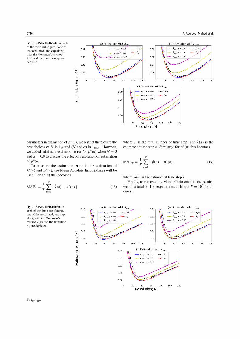
A. Abolpour Mofrad et al.
Fig. 8 SINE-1080-360. In eachof the three sub-figures, one ofthe max, med, and exp alongwith the Oommen’s methodλ(n) and the transition λtr aredepicted
parameters in estimation of p∗(n), we restrict the plots to thebest choices of N in λtr, and (N and α) in λmax. However,we added minimum estimation error for p∗(n) when N = 5and α = 0.9 to discuss the effect of resolution on estimationof p∗(n).
To measure the estimation error in the estimation ofλ∗(n) and p∗(n), the Mean Absolute Error (MAE) will beused. For λ∗(n) this becomes
MAEλ = 1T
T∑
n=1
| λ(n) − λ∗(n) | (18)
where T is the total number of time steps and λ(n) is theestimate at time step n. Similarly, for p∗(n) this becomes
MAEp = 1T
T∑
n=1
| p(n) − p∗(n) | (19)
where p(n) is the estimate at time step n.Finally, to remove any Monte Carlo error in the results,
we ran a total of 100 experiments of length T = 105 for allcases.
Fig. 9 SINE-1080-10080. Ineach of the three sub-figures,one of the max, med, and expalong with the Oommen’smethod λ(n) and the transitionλtr are depicted
2710

On solving the SPL problem using the concept of probability flux
Table 2 Summary of the choices of tuning parameters resulting in minimum error for λtr and λmax in SINE Experiments. The smallest error valuein each experiment is represented in bold font
E–NISEstimator
1080–1080 360–360 1080–360 1080–10080
N Error N Error N Error N Error
Oommen(λ(n)) 80 0.04791 35 0.08634 65 0.05502 40 0.09244
LTES(λtr) 80 0.04682 35 0.08425 60 0.05363 40 0.08952
FES(λmax) α = 0.6 80 0.0471 35 0.08533 60 0.05377 40 0.08937
α = 0.7 80 0.04749 35 0.08659 60 0.05398 40 0.08935α = 0.8 75 0.0485 35 0.08965 60 0.0548 35 0.08959
α = 0.9 75 0.05106 35 0.09706 60 0.05733 35 0.09085
α = 0.95 75 0.05578 35 0.11246 55 0.06228 30 0.09474
α = 0.99 65 0.111 20 0.31157 30 0.12002 25 0.14673
4.1 Moderate changes of both λ∗(n) and p∗(n)
In this section both λ∗(n) and p∗(n) change moderately.Figure 1 shows the estimation error as a function ofresolution for some choices of α. At any resolution, λtr haslower estimation error than λ(n) and indeed, all the casesλmax, λmed, and λexp perform more efficiently than λ(n) for,at least, a specific choice of α.
We also note that, the higher resolution will not result ina smaller error in all the cases. For instance, for λ(n), theestimation error increases after resolution N = 65 in whichthere is a minimum of errors. As it is represented in Table 1,the minimum error for λ(n) equals e = 0.063149 whenN = 65. We reach error e = 0.061353 for λtr at resolutionN = 50. The best error for λmax is e = 0.059138 whenN = 50 and α = 0.9. The minimum error over all scenariosis e = 0.058559 which is achieved by λmed estimator whenN = 50 and α = 0.95.
Figure 2 shows the estimation error as a function ofresolution for some choices of α for SINE-1080-1080. Allthe curves have an optimum resolution point in which anyhigher resolution cause higher estimation error. In the SINE-1080-1080 case, λmax and λtr are best satisfying estimators.λtr with minimum error e = 0.04682 at N = 80, slightlyoutperforms λmax with minimum error e = 0.047095 at(N = 80, and α = 0.6).
4.2 Fast changes of both λ∗(n) and p∗(n)
Here the effect of faster changes in λ∗(n) and p∗(n) areaddressed through cases SWITCH-100-100 and SINE-360-360.
Figure 3 is devoted to SWITCH-100-100 that both λ∗(n)and p∗(n) randomly switch to a new value in their domain.As expected, comparing the error with the SWITCH-1000-1000 case, the estimation errors are higher. From Table 1we see that the minimum error for the estimators λ(n), λtr,
and λmax are e = 0.1069, e = 0.10258, and e = 0.1021respectively. The minimum error in case SWITCH-100-100equals to e = 0.1021 and is achieved by λmax when N = 20and α = 0.6
As expected, we see that faster changing Environmentcould be tracked more accurately with smaller values ofresolution and α. For instance, compare resolution N = 20in this case, for λmax, to N = 50 in case SWITCH-1000-1000. The same comparison between α = 0.9 and 0.6 showsthat to track faster changing Environment we must rely onless on memory.
In Fig. 3, we observe that the best choice of α isdependent on the resolution; for example, if N = 5, theλmax, λmed, and λexp with α = 0.95 and α = 0.9 are superiorto the choices with α = 0.6. However N = 15, α = 0.6would be a more desirable option.
Regarding fast changes, Fig. 4 is devoted to SINE-360-360 in which both λ∗(n) and p∗(n) change continuouslyas a sine function with period 360 degree. The minimumerror in this case equals e = 0.08425 that is achieved byλtr at N = 35. Again, the simpler estimator λtr outperformsλmax with minimum error e = 0.085329 when (N =35 and α = 0.6). Note that, the λmax estimator is moreefficient than λ(n) that has minimum error e = 0.08634when N = 35. In comparison with SINE-1080-1080, theestimated error is higher and the best resolution is muchsmaller in case SINE-360-360. Compare the best resolutionN = 35 to the case SINE-1080-1080 which equals toN = 80. Notice that α values closer to 1, produce weakerestimations.
4.3 Effect of changing rate of p∗(n) on estimationof λ∗(n) in SWITCH cases
In this section the effect of changing rate of p∗(n)on estimating λ∗(n) in SWITCH dynamic is examined.Two alternative cases SWITCH-1000-100 (Fig. 5) and
2711

A. Abolpour Mofrad et al.
SWITCH-1000-10000 (Fig. 6) are compared to SWITCH-1000-1000 (Fig.1). In Fig. 7 a trace plot for tracking λ∗(n)through LTES (λtr) is presented and the behavior of theestimator is discussed. Additionally, Table 1 summarizes thechoices of tuning parameters resulting into the minimumerror for λtr and λmax to the SWITCH cases.
From Fig. 5 and Table 1, we observe that estimatorsperform better in SWITCH-1000-100 in comparison withSWITCH-1000-1000. For instance, compare the minimumerror of estimator λtr in case SWITCH-1000-100 which ise = 0.03671 for N = 80 with e = 0.06135 for N = 50 incase SWITCH-1000-1000.
The minimum error in various settings is e = 0.03538which is achieved by λmed estimator when N = 75 andα = 0.9.
Figure 6 presents the case SWITCH-1000-10000 wherep∗(n) changes ten times slower than SWITCH-1000-1000.It is observable that estimators show a better performance incase SWITCH-1000-10000 compared with SWITCH-1000-1000. As presented in Table 1 we see that the minimumerror for the estimators λ(n), λtr, and λmax are e = 0.05027,e = 0.048795, and e = 0.04521 respectively. The bestestimator is λmax when α = 0.95 and N = 50.
In summary, the results, as shown in Figs. 5, 6, andTable 1, indicate that when the Environment effective-ness changes fast, the minimum estimation error will besmaller. Compare minimum errors e = 0.03539 to e =0.05914 and e = 0.04521 for cases SWITCH-1000-100,SWITCH-1000-1000, and SWITCH-1000-10000 respec-tively. However, the error in SWITCH-1000-10000 whenp∗(n) changes very slow is better than moderate changes inSWITCH-1000-1000. This result is somewhat counterintu-itive. In order to understand it, we compare the trace plots ofSWITCH-1000-100, SWITCH-1000-1000, and SWITCH-1000-10000 together in Fig. 7.
Figure 7 shows tracking λ∗(n) under optimal choicesof parameters for λtr in order to study the impact ofEnvironment effectiveness on estimation of λ∗(n). Forthe sake of simplicity, suppose there is a same chainλ∗(n) in all the cases. Consider λ∗(n) along with threeEnvironment effectiveness chains p∗
f (n), p∗m(n), and p∗
s (n),for SWITCH-1000-100 (fast changes), SWITCH-1000-1000 (moderate changes), and SWITCH-1000-10000 (slowchanges) respectively, in which their average value areapproximately the same i.e.
1T
T∑
t=1
p∗f (n) ≈ 1
T
T∑
t=1
p∗m(n) ≈ 1
T
T∑
t=1
p∗s (n).
Consider SWITCH-1000-10000 with p∗s (n) and let the
estimation of λ∗(n) be λ(n); suppose the following threescenarios:
1. The Environment effectiveness is close to 1, see n =60000 to n = 70000 in Fig. 7c. λ∗(n) is easily trackedin this segment and the estimation λ(n) is satisfactory.
2. The Environment effectiveness is slightly distant from1, but it is informative, see n = 70000 to n = 80000in Fig. 7c where p∗
s (n) value is close to 0.8. Becausethe information from Environment is somewhat faulty,tracking the point location in this segment is moredifficult, but still satisfactory.
3. The Environment effectiveness has a value close to 0.5,see n = 80000 to n = 90000 in Fig. 7c. The estimationλ(n) is unsatisfactory and it is almost a random chainwith a lot of fluctuations. The reason is that estimatordoes not receive new information from Environmentand after a short time λ(n) will deviate from λ∗(n).
In summary, we keep the well estimation in the firstsegment, the estimation performance is reduced in thesecond segment, but still satisfactory. Within the thirdsegment, possibility of error is rather high, and λ(n)fluctuates at a distant point from λ∗(n). For p∗
s (n) segmentslike the last one is discouraging, since we remain in anunsatisfactory situation for a long period of time.
Alternatively, consider the Environment effectivenessp∗f (n), Fig. 7a. It is possible to detect segments like the
above three segments but with a much shorter length. So,the behavior of λ(n) in each of them is not long lasting.Faster changes make the behavior of estimators more likethe second segment, with fluctuations around λ∗(n).
In Fig. 7b; i.e. SWITCH-1000-1000 case, the error isthe highest among the three cases. In this case, p∗
m(n) andλ∗(n) are changing at the same time. So, the changes ofp∗m(n) has no positive effect on estimation of λ∗(n). The
best resolution in this case equals N = 50, which suggestsmore changes than SWITCH-1000-10000 with N = 65 andSWITCH-1000-100 with N = 80. This smaller resolution,produces a higher error. To investigate the negative effectof the simultaneous changes more, we run the SWITCH-1000-1000 case where there is a 500 steps delay betweenλ∗(n) and p∗
m(n) changes. That reduces the minimum errorto e = 0.05144 for N = 65, and approves the negativeeffect of simultaneous changes in SWITCH cases.
The main observations in Fig. 7 are:
– Tracking λ∗(n) is heavily affected by Environmenteffectiveness. In Fig. 7c, there are no fluctuations whenp∗s (n) ≈ 1, however, when p∗
s (n) ≈ 0.8, the estimatorfluctuates more around the optimal λ∗(n), and thenwhen p∗
s (n) is slightly larger than 0.5 the fluctuationsare much more bigger.
– Faster changes in Environment effectiveness leads tobetter estimations of λ∗(n). Note that, the rate ofchanges must be regulated in a way that λ(n) can
2712

On solving the SPL problem using the concept of probability flux
Fig. 10 SINE-1080-1080. a andb subfigures show how theestimation tracks λ∗(n) whenthe argument of sine function isthe same by λtr and λmax ,respectively. The c and dsub-figures show the same whenthe argument of sine functiondiffer by π/2
converge to λ∗(n) when Environment effectiveness isclose to 1.
– When λ∗(n) and p∗(n) changes together, it is muchharder to track λ∗(n).
– Since the average values of Environment effectivenessin three cases are supposed to be the same, and the mostestimation error is produced in the third segment, thereis a better performance in case p∗
f (n) in total.
From Table 1, we observe that the best estimationsbelong to the case SWITCH-1000-100 and estimator λmax.
4.4 Effect of changing rate of p∗(n) on estimationof λ∗(n) in SINE cases
This section focuses on the SINE dynamic and presents theresults for the effect of changing rate of p∗(n) on estimatingλ∗(n). Two alternative cases SINE-1080-360 (Fig. 8) andSINE-1080-10080 (Fig. 9) are compared with SINE-1080-1080 (Fig. 2), and Table 2 summarizes the same data asTable 1 for SINE cases.
As reported in Table 2, the best estimation error forcase SINE-1080-360 (Fig. 8) is achieved through λtr atN = 60 which equals to e = 0.05363; compare to the
best estimation error for SINE-1080-1080 that equals e =0.04682. In contrast to the SWITCH case, we see that fasterchanges of probability does not result in smaller estimationerrors. We later explain that along with the rate of changes,another factor which plays a role is the phase of changes.In SINE-1080-1080 both λ∗(n) and p∗(n) are in phasebut in SINE-1080-360 they have different periods and cannot be in phase. The effect of this will be addressed inSection 4.5 in details. The final case, SINE-1080-10080 inFig. 9, provides a more clear insight.
In SINE-1080-10080, the changes are asymmetric andthe Environment effectiveness varies slower. The minimumestimation error equals e = 0.08935 and occurs for λmaxat (N = 40,α = 0.7). In this case, we observe that λmax
estimator slightly outperforms λtr. The minimum error forλtr is e = 0.08952 at N = 40. Moreover, λexp resultsthe best minimum error, e = 0.08835 when N = 35 andα = 0.6
By comparing SINE-1080-10080 with SINE-1080-1080and SINE-1080-360, we observe that its estimation error isthe weakest.
If only SINE-1080-360 and SINE-1080-10080 arecompared with together, we detect a better estimation at
Table 3 Summary of SINE-1080-1080 alternatives
n range θ range λ∗(n) range p∗1(n) range p∗
2(n) range
n1 − n2 (2kπ + π/4) − (2kπ + 3π/4) [0.85, 1] [0.93, 1] [0.57, 0.93]n2 − n3 (2kπ + 3π/4) − (2kπ + 5π/4) [0.15, 0.85] [0.57, 0.93] [0.93, 1]n3 − n4 (2kπ + 5π/4) − (2kπ + 7π/4) [0, 0.15] [0.5, 0.57] [0.57, 0.93]n4 − n5 (2kπ + 7π/4) − (2(k + 1)π + π/4) [0.15, 0.85] [0.57, 0.93] [0.5, 0.57]
2713

A. Abolpour Mofrad et al.
Fig. 11 Estimation of p∗(n)with binomial weak estimationvia two alternative choices ofλ∗(n) estimations (λmax and λtr)for SWITCH-1000-1000 a,SWITCH-100-100 b,SWITCH-1000-100 c, andSWITCH-1000-10000 d
faster changing Environment effectiveness. While SINE-1080-1080 is not following this hypothesis. In contrastto SWITCH cases, where moderate changes of p∗(n)in SWITCH-1000-1000 show the weakest performance,moderate changes of p∗(n) in SINE-1080-1080 show thebest results. This suggests that another factor affects theestimation. Later in Section 4.5, Fig. 10, we explain itthrough the assessment of two different trace plots forSINE-1080-1080 case.
We have collected the best parameter values and resultedminimum errors of λ(n), λtr, and λmax in Table 2. Thebest estimations belong to the case SINE-1080-1080. Here,LTES estimator (λtr) is the best estimator.
4.5 The relation between λ∗(n) and p∗(n) changesand the estimation performance
To study the effect of the relation between λ∗(n) andp∗(n) dynamics on the estimators, we consider the caseSINE-1080-1080 that both λ∗(n) and p∗(n) are changingaccording a sine curve. So, we re-run the SINE-1080-1080 case when the arguments of sine functions for λ∗(n)and p∗(n) differ by π/2. More formally, what we havereported on Fig. 2 and on the top of Fig. 10 is λ∗(n) =0.5 + 0.5 sin( π
3·180 ) and p∗(n) = 0.75 + 0.25 sin( π3·180 ).
In the second run, λ∗(n) argument is added by π/2, soλ∗(n) = 0.5 + 0.5 sin( π
3·180 + π/2) (Fig. 10c and d).
Fig. 12 Estimation of p∗(n)with binomial weak estimationvia two alternative choices ofλ∗(n) estimations (λmax and λtr)for SINE-1080-1080 a, SINE-360-360 b, SINE-1080-360 c,and SINE-1080-10080 dEnvironments
2714

On solving the SPL problem using the concept of probability flux
Table 4 Summary of tuning parameters resulting into minimum error, along with the parameters N = 5 and α = 0.9 for ptr and pmax. The lowesterror value among ptr and pmax for each case is represented in bold font
EstimatorCase
λtr λmax
N γ Error N α γ Error
SWITCH-1000-1000 50 0.97 0.08406 50 0.9 0.99 0.0524SWITCH-1000-1000 5 0.98 0.06812 5 0.9 0.99 0.04199SWITCH-100-100 20 0.92 0.10819 20 0.6 0.92 0.10819SWITCH-100-100 5 0.94 0.08967 5 0.9 0.95 0.07445SWITCH-1000-100 80 0.94 0.10135 75 0.9 0.94 0.08126SWITCH-1000-100 5 0.94 0.08697 5 0.9 0.95 0.07086SWITCH-1000-10000 65 0.95 0.10736 50 0.95 0.999 0.04036SWITCH-1000-10000 5 0.999 0.08444 5 0.9 0.999 0.0399SINE-1080-1080 80 0.94 0.11103 80 0.6 0.94 0.11103SINE-1080-1080 5 0.97 0.06308 5 0.9 0.97 0.05056SINE-360-360 35 0.92 0.125 35 0.6 0.92 0.125SINE-360-360 5 0.94 0.077 5 0.9 0.94 0.07433SINE-1080-360 60 0.94 0.11201 60 0.6 0.94 0.11201SINE-1080-360 5 0.94 0.07282 5 0.9 0.94 0.06873SINE-1080-10080 40 0.99 0.08299 40 0.7 0.99 0.08299SINE-1080-10080 5 0.99 0.04871 5 0.9 0.99 0.0345SINE-1080-1080-Shift 25 0.97 0.07681 20 0.8 0.97 0.762SINE-1080-1080-Shift 5 0.97 0.0586 5 0.9 0.97 0.05437
Hereafter, we call it SINE-1080-1080-Shift. We observesignificant differences between tracking λ∗(n) throughoutthe two scenarios SINE-1080-1080 (Fig. 10a and b) andSINE-1080-1080-Shift (Fig. 10c and d). The estimatorsλtr and λmax track λ∗(n) more accurately in SINE-1080-1080 than SINE-1080-1080-Shift. Moreover, the minimumestimation error for λtr in SINE-1080-1080-Shift is e =0.10504, while it equals to e = 0.04682 for λtr in SINE-1080-1080. Similarly, the minimum estimation error forλmax in SINE-1080-1080-Shift is e = 0.10382. Compare itto e = 0.0471 for λmax in SINE-1080-1080. We explain itby analyzing Fig. 10. In general, when λ∗(n) value is closeto 0 or 1, the effect of wrong guidance from Environment isreduced. The reason is that λ(n) cannot pass the boundaries.
Let λ∗(n) = 0.5 + 0.5 sin(θ), so we have p∗1(n) =
0.75+0.25 sin(θ) for SINE-1080-1080 and p∗2(n) = 0.75+
0.25 sin(θ − π/2) for SINE-1080-1080-Shift.Let us take the case SINE-1080-1080 where p∗(n) and
λ∗(n) are in phase, i.e. p∗(n) = p∗1(n) . Interestingly, the
valley of p∗1(n) corresponds to the valley of λ∗(n). Since
p∗1(n) has a valley around 0.5, then the tracking of λ∗(n)
will be handicapped during that period but this will notaffect much the accuracy as λ∗(n) is also experiencing avalley and the changes are slow over that valley. However,in case SINE-1080-1080-Shift where p∗
2(n) and λ∗(n) areout of phase, a valley of p∗
2(n) coincides with a change of
λ∗(n) from its lowest value to its biggest value. Then, duringthat valley of p∗
2(n), λ∗(n) tracking gets handicapped andthe error is big due to the scheme not being able to trackthe true underlying λ∗(n) that changes dramatically from itsmin to its max. To be more precise, let
θ1 = 2kπ + π/4, θ2 = 2kπ + 3π/4, θ3 = 2kπ + 5π/4,θ4 = 2kπ + 7π/4, and θ5 = 2(k + 1)π + π/4 where k is apositive integer. This way we divide a period of 1080 stepsto four equal parts each with 270 steps. For the above values,λ∗(n1) up to λ∗(n2) is situated in the range [0.85, 1]; i.e. in270 successive steps the point location is placed within thisrange. However, for the next 270 steps, i.e. from λ∗(n2) toλ∗(n3), the values locate in range [0.15, 0.85]. We observethat the rate of changes is not uniform. Similarly, λ∗(n3) toλ∗(n4) is placed in the range [0, 0.15] and λ∗(n4) to λ∗(n5)is situated in the range [0.15, 0.85].
Similar to the discussions we had about SWITCH cases,we have
1T
T∑
t=1
p∗1(n) ≈ 1
T
T∑
t=1
p∗2(n).
This time p∗1(n) and p∗
2(n) are exactly the same, but theirrelation to λ∗(n) makes them different.
2715

A. Abolpour Mofrad et al.
In range n1 to n2, where λ∗(n) is located in [0.85, 1],p∗1(n1) to p∗
1(n2) is situated in the range [0.93, 1]. In rangen2 to n3, where λ∗(n) is located in [0.15, 0.85], p∗
1(n2) top∗1(n3) is situated in the range[0.57, 0.93]. Moreover, in the
range n3 to n4, where λ∗(n) is located in[0, 0.15], p∗1(n3) to
p∗1(n4) is placed in the range [0.5, 0.57]. Finally, for range
n4 to n5, where λ∗(n) is located in [0.15, 0.85], p∗1(n4) to
p∗1(n5) is situated in the range [0.57, 0.93].The intervals for values of p∗
2(n) are achieved throughshifting p∗
1(n) values. When λ∗(n) is in range [0.85, 1] ittakes values in [0.57, 0.93], and when λ∗(n) is in range[0.15, 0.85] it takes values in [0.93, 1]. When λ∗(n) isplaced in range [0, 0.15] it takes values in [0.57, 0.93], andwhen λ∗(n) is placed in range [0.15, 0.85] it takes values in[0.5, 0.57]. See Table 3 for a summary:
A comparison of the two Environments reveals whyestimation of SINE-1080-1080 (p∗
1(n)) outperforms SINE-1080-1080-Shift (p∗
2(n)):
– In range n1 − n2, since p∗1(n) values are higher, we will
have more promising estimations. Note that p∗2(n) is in
range [0.57, 0.93], λ∗(n) is close to 1, when it reachesits peak, hence its value changes slowly. That is to sayin this period, estimations in SINE-1080-1080-Shift aresatisfactory. See, for instance, around n = 24500 inFig. 10c and d.
– In range n2 − n3, the changes in λ∗(n) are fast.Estimation in SINE-1080-1080 case is more difficultthan SINE-1080-1080-Shift, because p∗
1(n) is in range[0.57, 0.93] and p∗
2(n) is in range [0.93, 1].– In range n3 − n4, the changes in λ∗(n) are not fast and
the value is close to the boundary. p∗1(n) is in range
[0.5, 0.57] while the information from Environment isalmost random. However, since λ∗(n) is in a peak, itsvalue is close to boundary and does not change fast,as we explained before, the most fluctuations will benearby the true λ∗(n); see around n = 21000 in Fig. 10aand b. Tracking λ∗(n) changes in SINE-1080-1080-Shift case is more accurate than in SINE-1080-1080case.
– In range n4−n5, the changes in λ∗(n) are fast. Trackingλ∗(n) in SINE-1080-1080 Environment, similar to therange n2 − n3, is acceptable to some extent. However,tracking the point location in SINE-1080-1080-ShiftEnvironment is almost impossible. As can be seen inFig. 10c and d around n = 22500, the combinationof fast changes of λ∗(n) and distance from boundaries,cause huge deviation. Such periods result in higherestimation error in SINE-1080-1080-Shift Environmentthan SINE-1080-1080.
Therefore, both the rate of changes in Environmenteffectiveness and its relationship to the point location mightaffect the estimations.
4.6 Estimation of environment effectiveness: p∗(n)
In Figs. 11 and 12 the estimation error for various SWITCHand SINE cases are presented respectively. Moreover,Table 4 summarizes the choices of tuning parametersresulting into the minimum error while Environmenteffectiveness is estimated.
In order to depict the estimation performance of p∗(n),we restrict the results to estimation based on two casesλmax and λtr, for these are the main contribution in thispaper which perform the best. Moreover, we consider thebest parameters of these two estimators based on results ofprevious error plots. The tuning parameters resulted to thebest minimum error reported in Table 4. We will considerand discuss the results for N = 5 and α = 0.9 in Table 4later. In the following we will compare the results frombest λ∗(n) estimations. The best minimum error in caseSWITCH-1000-1000 is achieved for pmax when (N =50,α = 0.9 and γ = 0.99) equals to e = 0.0524. The errorfor alternative method, i.e. ptr equals to e = 0.08406 when(N = 50, and γ = 0.97), see Table 4.
The best minimum error in case SWITCH-100-100 issimultaneously achieved for pmax and ptr at value e =0.10819 with parameters (N = 20,α = 0.6, and γ =0.92). In comparison with SWITCH-1000-1000, it isweaker than the previous case in which Environmentchanges more slowly.
In case SWITCH-1000-100, the best minimum error isobtained through pmax when (N = 75,α = 0.9 and γ =0.94), that equals to e = 0.08126. Error for ptrequals to e = 0.10135 in the case (N = 80, andγ = 0.94).
Finally, the case SWITCH-1000-10000 where the mini-mum error for pmax when (N = 50,α = 0.95 and γ =0.999) equals to e = 0.04036. The error for alternativemethod ptr equals to e = 0.10736 in case that (N =65, and γ = 0.95).
Overall, it seems like λmax performs a little better thanλtr. However, a significant disadvantage of λmax comparedwith λtr is that the tracking of λ∗(n) requires tuning of twoparameters compared to only one for λtr. For dynamicallychanging environments it is usually hard enough to tune oneparameter.
In case SINE-1080-1080 illustrated in Fig. 12a, wechoose N = 80 for λtr and (N = 80,α = 0.6) for λmaxas the best parameters. As reported in Table 4, the bestestimation error for both pmax and ptr occurs at γ = 0.94and equals e = 0.11103.
Similarly, we observe that both estimators are equallywell for cases SINE-360-360, SINE-1080-360, and SINE-1080-10080; where the best estimation error equals to e =0.125, e = 0.11201, and e = 0.08299 respectively, seeTable 4 for more details.
2716

On solving the SPL problem using the concept of probability flux
Even though the estimation error for point locationin case SINE-1080-10080 is weaker than all the casesSINE-1080-1080, SINE-360-360, and SINE-1080-360, itsestimated probability is preferred; because slower changescan be tracked more easily.
In SINE cases, apart from the case SINE-1080-10080and SINE-1080-1080-Shift, the estimation error is poor, i.e.optimal error is greater than 0.1 in both ptr and pmax. InFigs. 11, 12 and Table 4, we see that in some cases ptr andpmax perform equally well, even though the estimators λtrand λmax results are different. The reason is in estimationof Environment effectiveness, the important data is whetherthe suggested direction by Environment agrees with theestimation or not. In other words the distance betweenestimation and the point location is not important, and thecrucial issue is that both point location and its estimation,are at the same side- left or right- of the query location. Sowe can have exactly the same results even if the estimatedpoint is not the same in two estimators.
A natural question that might arise is that whether thebest parameters for estimation of λ∗(n) are the best forestimating p∗(n) or not. A simple simulation, where we setN = 5 and α = 0.9, provides a negative answer to thisquestion. These parameters result into a smaller estimationerror for all the cases compare to the best parameters.Moreover, the pmax estimations are all better than ptr. Forinstance, in case SWITCH-1000-1000 the estimation errorfor ptr drops from e = 0.08406 for N = 50, to e = 0.06812for N = 5. For pmax, error drops from e = 0.0524 to e =0.04199 for the same resolutions. Similarly, for SINE-1080-1080, please compare the error e = 0.11103 for N = 80and α = 0.6 to e = 0.06308 and e = 0.05056 for ptr andpmax respectively, when N = 5 and α = 0.9; see Table 4.We try to justify the reason behind this in the following.
Recall (4), (5), and (6) where we have:
πi = e.πi−1 whenever i ≤ Z ,
πZ+1 = πZ , and
πi =πi−1
ewhenever i > Z + 1,
where e = pq . To find a relation between resolution and π+
Zwe have:
1 =N−1∑
i=0
π+i
=Z−1∑
i=0
π+i +
N−1∑
i=Z+1
π+i + π+
Z (20)
By substituting the relations (7), (8), and (9):
= 2q
⎛
⎝Z−1∑
i=1
πi +N−1∑
i=Z+1
πi
⎞
⎠ + 2p(πZ )
= 2q πZ
⎛
⎝Z−1∑
i=1
(1e
)i
+N−1∑
i=Z+1
(1e
)i−Z⎞
⎠ + 2p(πZ ) (21)
By removing q and simplification:
= 2pπZ
[
1+ 1e2
(Z−2∑
i=0
(1e
)i
+N−2∑
i=Z
(1e
)i−Z)]
. So
πZ = 1
2p[1+ 1
e2
(∑Z−2i=0
(1e
)i+ ∑N−2
i=Z
(1e
)i−Z)] (22)
The above equation implies that for a static environmentthe larger N , the smaller πZ . Since for the estimation ofp∗(n) the accuracy of point location is not important, asmaller resolution will increase the probability to be at thecorrect pair, i.e. Z/N ≤ λ∗(n) < (Z + 1)/N . Basedon this argument, we can formally prove that a smallerresolution gives a better estimation of p∗(n) while a largerresolution yields a better estimation of λ∗(n). Based onthe above theoretical result that is in accordance with ourexperimental results, we therefore suggest to run the SPL inparallel using two different resolutions: a smaller resolutionfor better estimation of p∗(n) and a larger resolution forbetter estimation of λ∗(n).
4.7 Environment effectiveness tracking
The results of estimation of Environment effectivenessthrough tracking curves, which are depicted in Figs. 13 and14, are analyzed in this section.
Figure 13 compares tracking p∗(n) for two casesSWITCH-1000-100 (a-b) and SWITCH-1000-10000 (c-d)based on estimations λmax and λtr. We observe that ptrfluctuation is higher than pmax. Indeed, pmax documents alittle better peak performance (as the trace plots show), butat the price of requiring tuning of an additional parameter inλmax.
Moreover, as we see more clear at SWITCH-1000-10000case, whenever probability is closer to 1, any change inλ∗(n) intensely affects the p∗(n) estimators. So we detectsharper changes in p∗(n) estimators within the range ofn = 60000 to n = 70000. Then, there is a middle rangeprobability around 0.8 from n = 70000 to n = 80000.In this range estimators fluctuate more but change lessshapely. Interestingly, within the range of n = 80000 ton = 90000 there are fewer fluctuations. The reason is that
2717

A. Abolpour Mofrad et al.
Fig. 13 Comparison of how theestimators track p∗(n) withdifferent dynamics. Thesub-figures a and b show howλ∗(n) is tracked by λtr and λmaxrespectively in caseSWITCH-1000-100.Sub-figures c and d track λ∗(n)by λtr and λmax respectively, incase SWITCH-1000-10000. InSWITCH-1000-100 cases a sliceof Environment from n = 60000to n = 62000 are represented.The represented slice forSWITCH-1000-100 isn = 60000 to n = 90000
the Environment provides almost random directions andthe changes of λ∗(n) are not followed by the estimatorsefficiently. Since λ∗(n) estimation is the basis for p∗(n)estimation, the changes in λ∗(n) could not affect p∗(n)estimations. Therefore, there are no sharp changes whenp∗(n) is close to 0.5.
Even though the estimation error for point location incase SWITCH-1000-10000 is weaker than SWITCH-1000-100, its estimated probability is preferred; because slowerchanges can be tracked more easily.
Figure 14 compares tracking p∗1(n) with p∗
2(n) forSINE-1080-1080 and SINE-1080-1080-Shift, based ontwo estimations λmax and λtr. An interesting observation
regarding the Fig. 14 is the different behavior of estimationsnear value 1. The estimation for p∗
1(n) is more accuratecomparing to p∗
2(n), which can be explained due to thevalue of λ∗(n). The tracking is promoted by the fact thatin SINE-1080-1080 (Fig. 14a and b), λ∗(n) is both closeto 1 and changes more slowly. However, the tracking isweakened in SINE-1080-1080-Shift due to λ∗(n) changesfaster in the middle ranges. Through comparing the tworesults, it can be seen that although the estimation ofλ∗(n) is weaker in SINE-1080-1080-Shift, the proposedestimators for p∗(n) in SINE-1080-1080-Shift are moreprecise. Compare the minimum error e = 0.07681 inSINE-1080-1080-Shift to e = 0.11103 in SINE-1080-1080.
Fig. 14 SINE-1080-1080.Comparison of how theestimations track p∗(n), whenλ∗(n) and p∗(n) are eitherin-phase a–b, or out of phasec–d
2718

On solving the SPL problem using the concept of probability flux
Fig. 15 Trace plot for FES(Max) and LTES (Tr) fortracking the probability of thecurrent topic be News in topictracking experiment withkeyword list approach. Theblack curve show the offlineestimate
5 Real-Life experiment
In this Section, we show how our proposed algorithms canbe used for topic tracking in a stream of text by enhancingan existing estimator proposed in the literature [32]. Onlinetracking of topics in a stream of text, such as news/socialmedia feeds, has been addressed in several research [3, 8,25].
Consider News and Entertainment (including sports)as the two topics of interest. The aim is to modelthis problem such that the point location would be theprobability of current topic being News. This quantity hasthe characteristics of point location (λ∗(n)). Additionally,we need some guidance from Environment to be able torun the proposed algorithms. As we will explain in thefollowing, we can consider x(n) ∈ {0, 1} to be a stream
of zero and ones, where zero stands for Entertainment andone stands for News. So, x(n) is a Binomial variable andλ∗(n)- i.e. probability that the current topic is News- is theBernoulli parameter for each trial.
In [32], the Stochastic Search on the Line-basedDiscretized weak Estimator (SSLDE) is used to estimatethe parameters of a distribution, when these parameterschange with time. Note that in the distribution parameterestimation problem, the Environment is rather artificialand is constructed to suggest whether to increase ordecrease the current estimate. We follow the same methodas the SSLDE for the online tracking problem andcreate an artificial Environment that guides us to the pointlocation.
Recall that for resolution N , we have λ(n) ∈{0, 1/N , 2/N , · · · , i/N , · · · , (N−1)/N , 1}. The estimator
Fig. 16 Evaluation of FES(Max) and LTES (Tr) fortracking the News in feedexperiment in machine learningapproach. The black curve showthe offline estimate
2719

A. Abolpour Mofrad et al.
is assigned initially the value λ(0) = ⌊N/2⌋N . The updating
rules for SSLDE [32] depends on whether the currentestimate is greater or less than N/2. Suppose that λ(n) = i
Nand, as mentioned above, let x(n) be the Binomial variablethat takes zero or one at time n.
1. Case 1: [i ≥ (N/2)]:– If x(n) = 1 and rand() ≤ N
2·i :
E(n, i) = 1 → λ(n + 1) = min((i + 1), N )
N– Else:
E(n, i) = 0 → λ(n + 1) = i − 1N
2. Case 2: [i < (N/2)]:– If x(n) = 0 and rand() ≤ N
2(N−i) :
E(n, i) = 0 → λ(n + 1) = max((i − 1), 0)N
– Else:
E(n, i) = 1 → λ(n + 1) = i + 1N
where 0 ≤ rand() ≤ 1 is a uniform random numbergenerator. Now, we are able to track the probability of thecurrent topic be News by using the above suggestions byEnvironment.
5.1 Tracking problem
As mentioned above, News and Entertainment are thetwo topics we consider in this experiment. To generatethe text feed, a large set of related articles are collectedfrom the popular Norwegian newspaper site vg.no. Thearticles are shuffled randomly with the assumption that thealgorithm is unaware of when transitions between News andEntertainment take place. In the same line as in [8], basedon the stream of text, two methods are used for generatingbinary observations namely the keyword-list approach andthe Machine learning approach.
– Keyword lists. A keyword list is a set of words for eachtopic, here News and Entertainment. For generationof the keyword lists, the popular Pointwise MutualInformation criterion [17] is used. We assume that oneword at time is received from the News feed and thetask is to track the probability of the current topic of thetext stream is News. The best possible estimate based onthe keyword list approach is to compute the portion ofkeywords in each article that are News keywords. Thisapproach is called offline approach. The performance ofour algorithm can be compared to this offline approachand see how close our online estimates are to theoptimal offline approach.
Figure 15 shows the tracking of the probability thatthe current topic is News for FES (Max) and LTES (Tr)for the first 15000 words. The total number of keywordsin the experiment was 800400, while there was not afixed period for changing between topics. We see thatour algorithms are able to track changes in the Newsstream well. For instance, look at period n = 5000to n = 11000. A difference between these real datafrom the simulations in Section 4 is that here the rateof changes is not fixed. As we see in Fig. 15 the offlineestimate changes rapidly in some periods (for n = 2000to n = 5000) and does not change for a long period(n = 5000 to n = 11000). Since in average the datahas long fixed periods, the best achieved resolution isN = 185, which is better for the long periods.
It is worth mentioning that this tracking data canbe used as a classifier. Consider what we really wantto understand from the data is that if the current feedbelongs to the News or Entertainment. Indeed, therequired answer is if the probability of the current topicbe News is greater than 0.5 or not. Interestingly, forclassification application, the best resolution is muchsmaller, i.e N = 45. The reason is that for classification,the flexibility is much more important compared toaccuracy.
– Machine Learning. The most used approach toautomatically classify text into different classes liketopics or sentiment is to train a machine learner. Theprocess starts by dividing the training text stream inbatches of 20 words, each within one of the Newsor Entertainment topics. In the machine learningapproach, the documents (batches) were representedby word frequencies in a bag of word matrix. Thesebatches are used to train a machine learning model. Forthis experiment multinomial ridge regression [4] is usedthrough the glmnet package in R [27]. For the testingpart, the single words of the text stream were collectedinto batches of 20 words. Each batch in this phase wereclassified into one of the News or Entertainment topicsusing the trained multinomial regression model. Theprobabilities of the current topic were updated in thesame manner as for the keyword list approach.
Figure 16 shows the tracking of the probabilities for thedifferent topics for the machine learning approach. The totalnumber of batches was 189141 which we depict the trackingin the first 5000 batches. Data changes faster in the MLapproach and therefore the best resolution is much smaller;N = 35. We see that the fluctuations are greater than Fig. 15because of this smaller resolution, but in turn, it is moreadaptable with fast changes. Similar to the keyword list,if we use the algorithms for classification, the resolutionwill be even smaller; i.e. N = 11. So, being aware of that
2720

On solving the SPL problem using the concept of probability flux
there might be different best parameters in the estimationfor different applications is an important point.
6 Conclusion
A wide range of real-life problems can be modeled as a SPLproblem, especially when the Environment is considered tobe non-stationary. The random walk method, that Oommenpresented for solving the SPL problem, is known toconverge into a value arbitrarily close to the point location,when both resolution and time tend to infinity. Oommen’smethod simply discretizes the interval and performs acontrolled random walk on it. This paper is an extentionof the preliminary work presented [18] where we proposea new method to estimate the point location in the SPLproblem domain. In the current paper, we have introducedthe mutual probability flux concept and have proved thatFlux-based Estimation Solution (FES) and Last Transition-based Estimation Solution (LTES), as a special case, alwaysoutperform Oommen’s method. Moreover, we present amethod to estimate Environment effectiveness, p∗(n). Thissimple method could track the probability of receivingcorrect response from the Environment in tandem with theunknown location estimation.
Apart from theoretical proofs several experiments arepresented in order to understand the characteristics ofeach method. We argued that λtr, proposed in this paper,is equally simple but with better estimation performancethan Oommen’s method. λmax, λexp and λmed show betterestimation performance than λtr in low resolutions, but thiscomes at the price of tuning one additional parameter. Thissuggests that if we have no constraint on N , i.e. λ∗(n)represents a continuous quantity, we can tune just with Nand estimate with LTES. But in the case where freely tuningover N is not possible, tuning with α and using one of λmax,λexp, and λmed could provide more accurate estimations.
As experiments show, the tracking of λ∗(n) performsbetter when p∗(n) value is close to 1. The estimationperformance of λ∗(n) drops drastically when p∗(n) is closeto 0.5. This is as expected, since in case p∗(n) = 1, ourestimation procedure will be correct, i.e. λ(n) switches backand forth around the true λ∗(n). In contradiction, in the casep∗(n) is close to 0.5, we have more faulty feedback, and soan unsatisfactory estimation of λ∗(n).
Based on the results, we have also discussed when λ∗(n)value is close to 0 or 1, the effect of faulty guidancefrom Environment will be reduced to some extent andthe estimation is slightly better. Moreover, if p∗(n) takesthe same value in average, faster changes of p∗(n) arepreferable; with the condition that changes in p∗(n) areslow enough that estimator could converge into λ∗(n) whenp∗(n) is reaching to 1. In this case, faster changes interrupt
a long lasting weak estimation and bring the estimator backinto a more accurate value. However, if p∗(n) and λ∗(n)changes simultaneously, the positive effect of faster changesof p∗(n) is lost. We have also discussed that, not only therate of changes, but also the relation between λ∗(n) andp∗(n) affects the estimation error where p∗(n) representsreliability of the feedback from Environment. A satisfactoryestimation of p∗(n) informs us to what extent we can trustthe feedback and subsequently the estimations we have builtupon that.
Publisher’s note Springer Nature remains neutral with regard tojurisdictional claims in published maps and institutional affiliations.
References
1. Arntzen E, Steingrimsdottir HS (2014) On the use of variationsin a delayed matching-to-sample procedure in a patient withneurocognitive disorder. In: Braunstein SM, Swahn MH, PalmierJB (eds) Mental disorder. iConcept Press
2. Camp CJ, Foss JW, O’Hanlon AM, Stevens AB (1996) Memoryinterventions for persons with dementia. Appl Cogn Psychol10(3):193–210
3. De Santo M, Percannella G, Sansone C, Vento M (2004) Amulti-expert approach for shot classification in news videos.In: International conference image analysis and recognition, pp564–571. Springer
4. Friedman J, Hastie T, Tibshirani R (2010) Regularization pathsfor generalized linear models via coordinate descent. J Stat Softw33(1):1
5. Granmo O-C, John Oommen B (2010) Optimal sampling forestimation with constrained resources using a learning automaton-based solution for the nonlinear fractional knapsack problem.Appl Intell 33(1):3–20
6. Granmo O-C, John Oommen B (2010) Solving stochasticnonlinear resource allocation problems using a hierarchy oftwofold resource allocation automata. IEEE Trans Comput59(4):545–560
7. Guo Y, Ge H, Huang J, Li S (2016) A general strategy for solvingthe stochastic point location problem by utilizing the correlationof three adjacent nodes. In: IEEE international conference on datascience in cyberspace (DSC). IEEE, pp 215–221
8. Hammer HL, Yazidi A (2018) Parameter estimation in abruptlychanging dynamic environments using stochastic learning weakestimator. Appl Intell 48(11):4096–4112
9. Havelock J, Oommen BJ, Granmo O-C (2018) Novel distanceestimation methods using ?stochastic learning on the line?strategies. IEEE Access 6:48438–48454
10. Hossain MA, Parra J, Atrey PK, El Saddik A (2009) A frameworkfor human-centered provisioning of ambient media services.Multimed Tools Appl 44(3):407–431
11. Huang D-S, Jiang W (2012) A general cpl-ads methodology forfixing dynamic parameters in dual environments. IEEE Trans SystMan Cybern B (Cybernetics) 42(5):1489–1500
12. Jang YM (2000) Estimation and prediction-based connectionadmission control in broadband satellite systems. ETRI J22(4):40–50
13. Jiang W, Huang D-S, Li S (2016) Random walk-based solution totriple level stochastic point location problem. IEEE Trans Cybern46(6):1438–1451
14. Kelly FP (2011) Reversibility and stochastic networks. CambridgeUniversity Press, Cambridge
2721

A. Abolpour Mofrad et al.
15. Kpamegan EE, Flournoy N (2008) Up-and-down designs forselecting the dose with maximum success probability. Seq Anal27(1):78–96
16. Landauer TK, Bjork RA (1978) Optimum rehearsal patterns andname learning. In: Gruneberg MM, Morris PE, Sykes RN (eds)Practical aspects of memory. Academic Press, London, pp 625–632
17. Manning CD, Schutze H (1999) Foundations of statistical naturallanguage processing. MIT Press, Cambridge
18. Mofrad AA, Yazidi A, Hammer HL (2017) Solving stochasticpoint location problem in a dynamic environment with weakestimation
19. Randolph N (2013) Probability, stochastic processes, and queue-ing theory: the mathematics of computer performance modeling.Springer Science & Business Media, Berlin
20. Oommen BJ (1997) Stochastic searching on the line and itsapplications to parameter learning in nonlinear optimization. IEEETrans Syst Man Cybern B (Cybernetics) 27(4):733–739
21. Oommen BJ, Calitoiu D (2008) Modeling and Simulating adisease outbreak by learning a contagion parameter-based model.In: Proceedings of the spring simulation multiconference, pp547–555. Society for computer simulation international
22. Oommen BJ, Kim S-W, Samuel MT, Granmo O-C (2008) Asolution to the stochastic point location problem in metalevelnonstationary environments. IEEE Trans Syst Man Cybern B(Cybernetics) 38(2):466–476
23. Oommen BJ, Raghunath G (1998) Automata learning andintelligent tertiary searching for stochastic point location. IEEETrans Syst Man Cybern B (Cybernetics) 28(6):947–954
24. Oommen BJ, Raghunath G, Kuipers B (2006) Parameter learningfrom stochastic teachers and stochastic compulsive liars. IEEETrans Syst Man Cybern B (Cybernetics) 36(4):820–834
25. Oommen BJ, Rueda L (2006) Stochastic learning-based weakestimation of multinomial random variables and its applicationsto pattern recognition in non-stationary environments. PatternRecogn 39(3):328–341
26. Tao T, Tao H, Cai G, Li S (2013) ALidaptive step searchingfor solving stochastic point location problem. In: Internationalconference on intelligent computing. Springer, pp 192–198
27. R Core Team (2017) R: A language and environment for statisticalcomputing
28. Yazidi A, Granmo O-C, Oommen BJ, Goodwin M (2014) A novelstrategy for solving the stochastic point location problem using ahierarchical searching scheme. IEEE Trans Cybern 44(11):2202–2220
29. Yazidi A, Hammer H, Oommen BJ (2018) Higher-fidelity frugaland accurate quantile estimation using a novel incrementaldiscretized paradigm. IEEE Access 6:24362–24374
30. Yazidi A, Oommen BJ (2017) A novel technique for stochasticroot-finding: enhancing the search with adaptive d-ary search. InfSci 393:108–129
31. Yazidi A, Oommen BJ (2017) The theory and applications of thestochastic point location problem. In: 2017 international confer-ence on new trends in computing sciences (ICTCS). IEEE, pp333–341
32. Yazidi A, Oommen BJ (2016) Novel discretized weak estimatorsbased on the principles of the stochastic search on the lineproblem. IEEE Trans Cybern 46(12):2732–2744
33. Zhang J, Lu S, Zang D, Zhou M (2016) Integrating particleswarm optimization with stochastic point location method in noisyenvironment. In: 2016 international conference on systems, man,and cybernetics (SMC). IEEE, pp 002067–002072
34. Zhang J, Wang Y, Wang C, Zhou M (2017) Symmetricalhierarchical stochastic searching on the line in informative anddeceptive environments. IEEE Trans Cybern 47(3):626–635
35. Zhang J, Zhang L, Zhou M (2015) Solving stationary andstochastic point location problem with optimal computing budget
allocation. In: 2015 IEEE international conference on systems,man, and cybernetics (SMC). IEEE, pp 145–150
Asieh Abolpour Mofrad is athird year PhD student in [psy-chological] Behavior Analy-sis at Oslo Metropolitan Uni-versity (OsloMet), Norway.She has an academic back-ground in Applied Mathemat-ics and Computer Science.She obtained her Master’sdegree in Coding Theory andCryptography from Amirk-abir University of Technol-ogy, Tehran, Iran in 2011. Shestarted a PhD in Informaticsat University of Bergen (UiB),Norway at 2012. Within her
first PhD in Bergen, she has worked on Artificial Auto-AssociativeMemories inspired from Neural Networks using Coding Theory Tech-niques. In terms of her second PhD, she has worked on HumanMemory and Learning; focusing Techniques. In terms of her secondPhD, she has worked on Human Memory and Learning; focusinginterested in Brain, Mechanisms of Memory, and Learning.
Anis Yazidi received the M.Sc.and Ph.D. degrees from theUniversity of Agder, Grimstad,Norway, in 2008 and 2012,respectively. He is currently anAssociate Professor with theDepartment of 2008 and 2012,respectively. He is currently anAssociate Professor with theDepartment of 2008 and 2012,respectively. He is currently anAssociate Professor with theDepartment of machine lear-ning, learning automata, sto-chastic optimization, software-defined networks and cloud
computing. He led the research group Autonomous Systems andNetworks at OsloMet from 2015 to 2018. He is currently the leader ofthe research group Applied Artificial Intelligence at OsloMet.
Hugo Lewi Hammer receivedthe M.Sc. and Ph.D. degreesfrom the Norwegian Univer-sity of Science received theM.Sc. and Ph.D. degrees fromthe Norwegian University ofScience received the M.Sc.and Ph.D. degrees from theNorwegian University of Sci-ence received the M.Sc. andPh.D. degrees from the Nor-wegian University of Sciencereceived the M.Sc. and Ph.D.degrees from the NorwegianUniversity of Science automa-ta and stochastic optimization.
2722

Study IV
Balanced Difficulty Task Finder: An Adaptive
Recommendation Method for Learning Tasks Based
on the Concept of State of Flow
Anis Yazidi, Asieh Abolpour Mofrad, Morten Goodwin, Hugo L. Hammer
and Erik Arntzen
Yazidi, A., Mofrad, A. A., Goodwin, M., Hammer, H. L., & Arntzen, E. (2020). Balanced
Difficulty Task Finder: An Adaptive Recommendation Method for Learning Tasks Based
on the Concept of State of Flow. Cognitive Neurodynamics.
204

RESEARCH ARTICLE
Balanced difficulty task finder: an adaptive recommendation methodfor learning tasks based on the concept of state of flow
Anis Yazidi1 • Asieh Abolpour Mofrad1 • Morten Goodwin2 • Hugo Lewi Hammer1,4 •
Erik Arntzen3
Received: 31 December 2019 / Revised: 24 May 2020 / Accepted: 1 June 2020� The Author(s) 2020
AbstractAn adaptive task difficulty assignment method which we reckon as balanced difficulty task finder (BDTF) is proposed in
this paper. The aim is to recommend tasks to a learner using a trade-off between skills of the learner and difficulty of the
tasks such that the learner experiences a state of flow during the learning. Flow is a mental state that psychologists refer to
when someone is completely immersed in an activity. Flow state is a multidisciplinary field of research and has been
studied not only in psychology, but also neuroscience, education, sport, and games. The idea behind this paper is to try to
achieve a flow state in a similar way as Elo’s chess skill rating (Glickman in Am Chess J 3:59–102) and TrueSkill
(Herbrich et al. in Advances in neural information processing systems, 2006) for matching game players, where ‘‘matched
players’’ should possess similar capabilities and skills in order to maintain the level of motivation and involvement in the
game. The BDTF draws analogy between choosing an appropriate opponent or appropriate game level and automatically
choosing an appropriate difficulty level of a learning task. This method, as an intelligent tutoring system, could be used in a
wide range of applications from online learning environments and e-learning, to learning and remembering techniques in
traditional methods such as adjusting delayed matching to sample and spaced retrieval training that can be used for people
with memory problems such as people with dementia.
Keywords Adaptive task difficulty � State of flow � Intelligent tutoring system � Game ranking systems � Online learning �Adjusting delayed matching-to-sample � Computerized adaptive testing � Stochastic point location
Introduction
Attempts to achieve computer tutoring systems that are as
effective as human tutors can be traced back to the earliest
days of computers (Smith and Sherwood 1976). Online
learning is becoming a significant driving force in today’s
educational systems. The lack of faculty members is a
common trend in today’s universities which makes per-
sonalized one to one teaching challenging, or practically
impossible. Students may struggle to fulfill their full
potential because the assigned tasks are generic and not
tailored to their specific needs and skill level. Several
studies show that personalized learning is the key to
increased fulfillment of potential (see, e.g., Miliband 2004).
A possible solution to the latter problem is resorting to the
advances in AI in order to personalize the teaching process.
AI could be defined as: ‘‘The automation of activities that
we associate with human thinking, activities such as
Anis Yazidi and Asieh Abolpour Mofrad have contributed
equally to this work.
& Anis Yazidi
Asieh Abolpour Mofrad
1 Department of Computer Science, Oslo Metropolitan
University, Oslo, Norway
2 Department of Computer Science, University of Agder,
Kristiansand, Norway
3 Department of Behavioral Science, Oslo Metropolitan
University, Oslo, Norway
4 Simula Metropolitan Center, Oslo, Norway
123
Cognitive Neurodynamicshttps://doi.org/10.1007/s11571-020-09624-3(0123456789().,-volV)(0123456789().,- volV)

decision-making, problem solving and learning’’ (Bellman
1978).
Some of early studies that allude to the term Intelligent
Tutoring System (ITS) dates back to 1982, where D. Slee-
man and J.S Brown pioneered the idea of a system
designed to help students reach their full potential in a
limited amount of time (see Sleeman and Brown 1982). A
few years later, a study is published demonstrating that
individual tutoring is twice as effective as group teaching
(Bloom 1984). Later, online e-learning platforms such as
Kahn Academy1 and Udemy,2 massive open online course
(MOOC) such as MIT OpenCourseWare,3 digital hand in
tools like Fronter, plagiarism controls like Ephorus
(Fronter), and autograding assignment tools such as Bak-
pax4 have emerged. True ITS also exists with open tools
like Codeacademy5 and other e-learning platforms.
ITSs can raise student performance beyond the level of
traditional classes and even beyond the level of students
who learn from human tutors (see Kulik and Fletcher 2016,
for a survey). A recent study by Chirikov et al. (2020)
shows that online education platforms could scale high-
quality science, technology, engineering, and mathematics
(STEM) education through national online education plat-
forms at universities. Such instruction can produce similar
learning outcomes for students as traditional, in-person
classes with a much lower cost (see also VanLehn 2011, for
a review of relative effectiveness of human tutoring,
intelligent tutoring systems, and other tutoring systems or
no tutoring).
An ITS is supposed to ‘‘provide immediate and cus-
tomized instruction or feedback to learners’’ (Psotka et al.
1988). In this paper, we provide algorithms that aspire to
fulfill the latter statement for the purpose of task selection.
Many ITSs are based on Computerized Adaptive Testing
(CAT) which is a form of computer-based test in which the
correctness of the student’s responses shapes the difficulty
level of upcoming tasks (see, e.g. Hatzilygeroudis et al.
2006; Kozierkiewicz-Hetmanska and Nguyen 2010; Jansen
et al. 2016, for instance). The aims of testing and practic-
ing through tutoring differ; testing should efficiently esti-
mate the student’s ability (Birnbaum 1968; Eggen and
Verschoor 2006), while training and practicing need to
consider motivation and involvement of students in line
with the length of the test (Jansen et al. 2016). A proba-
bility of success of 0.5 could minimize the test length, but
this level of challenge could be frustrating for some stu-
dents. For instance, in Math Garden, which is a web-based
application for monitoring and practicing math skills based
on CAT principles (Klinkenberg et al. 2011), a success
rate of 75% is considered on average.
There is a substantial body of work on Learning Auto-
mata (LA) and ITSs (see, e.g. Oommen and Hashem 2013).
In simple terms, LA is a stochastic machine attempting to
find the optimal strategy from a set of actions in a random
environment. LA, as a fundamental problem in AI, is
particularly important in decision making under uncer-
tainty (see Narendra and Thathachar 2012, for an intro-
duction to LA). The term tutorial-like systems refers to
study tutorial systems while no entity needs to be a real-life
individual. Research in this field tries to model components
of the system with appropriate learning models, such as
LA (Oommen and Hashem 2013).
In a tutorial-like system, the teacher also might be
stochastic and learns through the process of training
(Hashem 2007). The design and analysis of a tutorial-like
system model could involve modeling of a student (Oom-
men and Hashem 2009b), modeling of a classroom of
students where artificial students can interact and learn
from each other as well as the teacher (Oommen and
Hashem 2009a), modeling of a (stochastic) teacher
(Hashem and Oommen 2007), modeling the domain
knowledge (Oommen and Hashem 2010), and modeling
how teaching abilities of a teacher can be improved
(Oommen and Hashem 2013).
ITSs can also be applied in some traditional learning
methods in behavior analysis such as titrated delayed
Matching-to-Sample (MTS) method, also referred as
adjusting delayed MTS (Cumming and Berryman 1965;
Sidman 2013).6 Titrated delayed MTS has been used to
study remembering in a variety of settings, including to
study important variables in analyzing short-term memory
problems (Arntzen and Steingrimsdottir 2014). Similar
applications of ITSs in MTS and titrated delayed MTS
procedures, can proposed to the computational models of
these experimental methods which are usually introduced
in the sake of research (see, e.g. Mofrad et al. 2020, for a
recent computational model that simulates MTS proce-
dure). ITSs can be used as a tool in the simulation part of
training phase of MTS or titrated delayed MTS procedures
to study the effect of adaptive training in a simulator
model.
1 www.khanacademy.com.2 www.udemy.com.3 https://ocw.mit.edu.4 www.bakpax.com.5 www.codecademy.com.
6 Matching-to-sample procedures, have been frequently used to study
complex human behavior (see for instance Cumming and Berryman
1965; Sidman 1994). Arntzen (2012) provides an overview of MTS
experiments and several variables that can be manipulated when
designing an experiment through MTS procedures. In adjusting
delayed MTS, the length of the delay changes as a function of the
participants’ responses, which makes it similar to the adaptive task
assignment problem.
Cognitive Neurodynamics
123

Spaced retrieval training (SRT) (Camp et al. 1989) is
another method of learning and retaining a piece of infor-
mation by recalling that piece of information over
increasingly longer intervals. The underlying problem in
SRT is also similar to the adaptive difficulty task assign-
ment which is addressed here. The SRT method is espe-
cially used for people with dementia (Camp et al. 1996).
Note that defining or measuring task difficulty can be
addressed in many ways. A definition based on whether or
not a task is performed, has applications in developmental
research. In this context, easier tasks can be performed at
earlier stages of development (see, e.g. Gilbert et al. 2012).
For healthy adults, a difficult task can be defined as a
quantitative measure, say percentage of task compliance in
a series of trials. Response time is another measure of task
difficulty, where a longer response time in average is
equivalent to a more difficult task. Accuracy and response
time, however, trade against each other (Fitts 1966;
Wickelgren 1977) and both must be considered in a well-
defined and standard task difficulty measure. Difficult tasks
in this respect, can be defined as those with long response
time and and/or high frequency error (see, e.g. Gilbert et al.
2012, for other accounts in defining task difficulty).
In this paper, we present a formal theory by which an
ITS can select the difficulty of task in a similar manner to
selecting an opponent of similar capabilities in balanced
difficulty game (Herbrich et al. 2006), which is called
Balanced Difficulty Task Finder (BDTF). As suggested by
systems such as Elo’s chess skill rating (Glickman 1995)
and TrueSkill (Herbrich et al. 2006) for matching game
players, matched players should have similar capabilities
and skills in order to achieve a balance between skills and
challenges to experience the state of flow. We draw anal-
ogy between choosing an appropriate opponent or appro-
priate game level and automatically choosing an
appropriate level of a learning task. It is noteworthy that by
way of analogy, we can model the student as the player and
the chosen task by the system as the opponent.
Paper organization
The remainder of this paper is organized as follows. ‘‘State
of art’’ section reviews the state of the art and various
approaches to ITS modeling. ‘‘Modeling task selection as
balanced game using balanced difficulty task finder’’ sec-
tion models task selection as balanced difficulty game by
resorting to our devised BDTF. ‘‘The concept of flow’’
section addresses the concept of flow from psychological
point of view. In ‘‘Related work on games’’ section, related
works from research on games are reported. ‘‘Neural basis
of adaptive learning and state of flow experience’’ section
addresses some literature on neural basis of adaptive
learning and state of flow. Furthermore, theoretical
formulation of BDTF is provided in ‘‘Formulating learning
as a balanced difficulty game’’ section. Experimental
results in ‘‘Experimental results’’ section catalogues the
convergence properties of the BDTF discussed in the the-
ory part. Finally, concluding remarks and future works are
addressed in ‘‘Conclusions and future work’’ section.
State of art
In this section, relevant studies and papers are discussed to
give the reader an overview over the current state of the art.
Although several papers on this topic exist dating back
several years, the literature reviewed in this section is
limited to content published (preferably) after 2005.
There are several approaches to create an ITS. In the
most recent papers, we are presented with a mix of dif-
ferent artificial intelligence approaches to solve the prob-
lem. Common for most of the papers reviewed is the need
for a model of student including different properties like
learning-rate, previous experience and knowledge, and
other variables. An approach for such a model (from now
referred to as the student model) is represented in numerous
studies (see for instance Brusilovsky and Millan 2007;
Clement et al. 2014, 2015; Millan et al. 2010).
The use of the student model in recent papers suggests
that this approach is fairly common in the field of ITS.
Even though the model itself is fairly common, the
implementation varies significantly. As an example, Cle-
ment et al. (2015) resort to a combination of a student
model and a cognitive model to create a tutoring model.
With this approach, the authors try to eliminate the need for
a strongly typed student model. The goal is to adjust the
learning tasks to individual students with as little infor-
mation as possible. The use of a Learning Automata (LA)
algorithm enables the system to find the optimal learning
sequence for a specific student subject to some constraints;
such as requiring certain activities to happen before others.
A disadvantage of the latter approach is particularly the
assumption that some tasks should be carried out in an
order. The authors (Clement et al. 2015) assume that after
task A1, either A2 or B1 need to follow. If students move
to B1, they can not move back to any task in A category.
This is in most cases a simplification of the learning pro-
cess, since students should be able to work on several
categories and practice by repeating previous categories.
Clement et al. (2015) use partial-observable Markov
decision process (POMDP) for optimization of task
selection, which is inspired by Rafferty et al. (2011) who
used the students acquisition level to propose activities.
This method requires the system to assume all students
learn in the same way. It is also stated that this approach
can be optimal, but requires sophisticated student and
Cognitive Neurodynamics
123

cognitive models. In most cases these methods are based on
knowledge tracing-methods (KTM) which attempt to esti-
mate student knowledge in a parametric manner. Usually,
the lack of data causes this form of modeling to be inac-
curate. POMDPs also has been suggested to be used for
modeling a population of students, instead of individuals.
This approach has been proven to be suboptimal in an ITS
setting (Clement et al. 2015; Lee and Brunskill 2012).
On the other hand, several improved versions of the
KTM have been proposed in the literature. A Representa-
tive example is the Bayesian knowledge tracing (BKT) with
skill-specific parameters for each student. There are strong
indicators that BKT models accounting for the student
variance is superior to the Bayesian knowledge model
(Pardos and Heffernan 2010; Yudelson et al. 2013). This
partially nuances the criticism proposed by Clement et al.
(2015).
A significant number of studies indicate that intrinsically
motivated students perform better. Thus, this requires a
good ITS keeps motivating the student throughout the
whole learning experience. Lumsden (1994) investigated
the optimal strategy for motivating the student, and found
that one of the main keystones for a motivational experi-
ence is task mastery. This is backed up by Clement et al.
(2015) who proposes a solution where the student is pre-
sented with tasks that are neither too easy nor too hard, but
slightly beyond their current abilities. Psychologists refer
to this experience as state of flow (see, e.g. Csikzentmi-
halyi 1996).
In this article, we propose a solution where each student
starts with a predefined optimal-difficulty (Clement et al.
2015) which will be adjusted over time based on the stu-
dent answers. Some students may be more prone to be
motivated with challenging tasks, and therefore the overall
learning outcome may be more effective for these students.
On the other hand, we might find students struggling with
the default or optimal-difficulty. In such cases, the learn-
ing-rate should be decreased, allowing these students to
participate at a slower pace.
There are several possible alternatives to design an ITS.
We have looked at several candidates in this study,
including multi-armed bandits (Clement et al. 2015),
Bayesian-networks (Millan et al. 2010) and neural-net-
works (Zatarain Cabada et al. 2015), each with its own
advantages. As mentioned earlier the student model is an
important part of this ITS. In the latter reviewed papers, the
neural network and Bayesian-network both relied on
comprehensive student models, with a solid core of data in
order to be able to draw accurate assumptions and deci-
sions. These systems are shown to be reliable and effective,
but comprehensive data models are required in order to
achieve optimal operation (Clement et al. 2015). With the
use of LA it is possible to eliminate the need for prior-
knowledge about the students. The LA is efficient, and it
requires a weaker link between student and the cognitive
model. Clement et al. (2015) propose an LA for seven to
eight years old school-children learning to decompose
numbers while manipulating money. Even though a generic
solution is presented by Clement et al. (2015) relying
on multi-armed bandit, there is no evidence that a similar
approach is viable for use for adults and contexts addressed
in online learning (see also Hashem and Oommen 2007;
Hashem 2007; Oommen and Hashem 2009a, b, 2010, 2013,
for LA based models for a generalized framework of
tutoring system, called tutoring-like systems).
A limited number of studies describe the use of ITS in
programming courses. As representative studies, we iden-
tified Java Sensei (Zatarain Cabada et al. 2015) and ASK-
ELLE (Jeuring et al. 2012), each of the latter studies use a
different machine learning approach. Java Sensei resorts to
a combination of neural-network strategies and emotion
sensors to register information and to make decisions based
on input. ASK-ELLE ITS utilizes a domain reasoner using
a Haskel Compiler called Helios. This compiler was
developed to give feedback on wrong syntax. The system
requires each student to complete a given task, but helps
the student to accomplish the tasks by giving hints and
examples relevant to found error(s).
Before moving to the model and contribution of this
paper, we refer to the Stochastic Point Location (SPL)
problem which has some similarities to the current work. A
considerable amount of literature has been published on
SPL since the Oommen work (Oommen 1997) (see for
instance Yazidi et al. 2014; Mofrad et al. 2019). In SPL, an
LA search for a point location in a line through the guid-
ance of an external environment which might give faulty
advice. Many scientific and real-life problems can be
modeled as the instances of SPL problem, including
adaptive task assignment problem. For instance, in Mofrad
et al. (2019), some authors of this paper discuss that the
point location can represent the difficulty level of a task
that a participant can handle, and tries to find that point as
fast and accurate as possible. The participant performance
in Mofrad et al. (2019) is modeled using a stair function
with two levels: a high performance for difficulties under
the optimal manageable difficulty level and a low perfor-
mance for difficulties just above the same level, i.e., the
manageable optimal difficulty level. However, if we rather
use a more realistic performance function according to
which the performance is continuous and monotonically
decreases as a function of the difficulty level, the approach
proposed in Mofrad et al. (2019) will basically converge to
difficulty level for which the participant performance is at
50% under some mild conditions. In other words the model
finds a manageable difficulty level and can be used in
titrated delayed MTS, SRT and online environments. Such
Cognitive Neurodynamics
123

remark motivated the current study in which we resort to
the latter realistic performance model, for efficiently find-
ing a higher rates of performance that are motivating
enough for the learner, and provides a balance between
challenge and skills, usually above 50% such as 70%. In
comparison with Mofrad et al. (2019), where the adjust-
ment technique is symmetric, in the current work the effect
of correct and incorrect responses are not the same, i.e. the
adjustment is asymmetric.
Modeling task selection as balanced gameusing balanced difficulty task finder
In this section, we present BDTF as the main contribution
in this article which is a theory that aspires to learn the
appropriate difficulty of a task rather than exploring dif-
ferent types of tasks as in the case of work in Andersen
et al. (2016). Although both approaches can be combined,
we clearly distinguish between them as the second case can
be seen as a novel theory for determining the adequate
difficulty level of an assignment for the purpose of keeping
the learning activity motivating and not exploring (as in
Andersen et al. (2016), which is more concerned about
exploring the different tasks in a similar manner to bandit
problem).
Difficulty is a subjective concept, or more precisely, it is
more individual and personal (see, e.g. Gilbert et al. 2012).
We argue that difficulty should be tailored to the ability of
the student. In fact, as in video games, or chess, the player
is motivated by an appropriate level of challenge or
equivalently difficulty. For example, the purpose of Xbox
TrueSkill system (Herbrich et al. 2006) is to match players
that have similar capabilities so that the outcome of the
game is unpredictable (optimally equi-chance of winning
and losing). Elo tries to find a global ranking among
players and TrueSkill is similar to the Elo rating system for
matching chess players. We advocate that, in a similar
manner to TrueSkill and Elo, a student needs to find an
enough challenging assignment that matches his
capabilities.
After a brief introduction on psychological concept of
flow experience (‘‘The concept of flow’’ section), review-
ing related works on games (‘‘Related work on games’’
section), and related works addressing neural basis of
adaptive task difficulty and the state of flow (‘‘Neural basis
of adaptive learning and state of flow experience’’ section),
we provide a sound mathematical formulation (‘‘Formu-
lating learning as a balanced difficulty game’’ section) that
emanates from the field of stochastic approximation
(Kushner and Yin 2003).
The concept of flow
The history of optimal human functioning in humanistic
and health psychology can be tracked back to the work of
Maslow (1959) who refereed to these moments of self-
actualization peak experiences. These experiences are
described as instances of happiness, fulfillment, and
achievement with a feeling of awareness to one’s human
potential. Csikzentmihalyi (1996) has described such an
experience as a state of flow since it is characterized by ‘‘an
almost automatic, effortless, yet highly focused state of
consciousness’’ (p. 110).
Any mental or physical activity, according to
Csikzentmihalyi (1996), can generate flow if: it is a chal-
lenging enough task that requires intense concentration and
commitment, involves clear goals, provides immediate
feedback, and is perfectly balanced to the skill level of the
person.
Delle Fave and Massimini (1988) discuss that balancing
challenges and skills is not enough for optimizing the
quality of experience and the notion of skill stretching
inherent in the flow concept. They redefined flow as the
balance of challenges and skills at the time both are above
average levels for the person. Moreover, the quality of
experience intensifies in a channel by moving away from a
person’s average levels in the challenge/skills space. Fig-
ure 1 depicts a classification of experiences based on the
level of challenge and skill in eight categories. The rings
depict increasing intensity of experience in each channel or
Fig. 1 Model of the flow state adapted from Csikszentmihalyi (2020).
Perceived challenges and skills must be above the person average
level in order to experience a state of a flow. The apathy is the case
when both are below the average and the experience intensity is
increased by distancing from average, shown by rings
Cognitive Neurodynamics
123

quadrant (see Nakamura and Csikszentmihalyi 2014, for a
detailed overview of the concept of flow).
Related work on games
A representative study that sheds light on the relationship
between three inter-related concepts: difficulty, motivation
and learning is presented by Chen (2007) that introduces
the flow Channel to the filed of games. According to Schell
(2014) and Chen (2007), when the difficulty exceeds the
learner’s skill, the learner experience a feeling of anxiety at
the thought of his learning skills are insufficient, and as a
result gets demotivated. Consequently, the learner tends to
abandon the activity after short time. On the other hand,
boredom takes place in the other extreme case where the
student level is much higher than the assignment’s diffi-
culty. In this sense, the student perceives the assignment as
a waste of time. The ideal case according to Schell (2014)
and Chen (2007) takes place when the aptitude of the
learner and the difficulty level are in state of balance. In
this case, similar to the psychological definition of flow, the
learner is said to achieve a state of flow. Chen (2007)
defines the flow as: ‘‘the feeling of complete and energized
focus in an activity, with a high level of enjoyment and
fulfillment’’.
As reported by Gallego-Duran et al. (2016), the notion
of difficulty in games does not seem to have attracted much
attention in the field of education in general. In this per-
spective, the proposed BDTF tries to bridge the gap
between two seemingly disjoint fields of research, namely,
ITSs and game ranking/matching systems.
The most pertinent work to our approach emanates from
the realm of computer games and chess where it was
remarked that when the level of the game is either too
difficult or too easy, the players abandon playing (Chen
2007; Schell 2014). Extensive literature has been centred
on the design of adaptive method to adjust the difficulty of
the game so that to match the level of the players, but in the
interest of brevity, we skip them (see, e.g. Hunicke 2005).
Neural basis of adaptive learning and stateof flow experience
There are many studies on the neural basis of state of flow
that we briefly review some of them. Due to the complexity
of concept of flow, it must be measured through its com-
ponents. Dietrich (2004) analyses the flexibility/efficiency
trade-off in the flow state and concludes that a prerequisite
to the experience of flow period is ‘‘a state of transient
hypofrontality that enables the temporary suppression of
the analytical and meta-conscious capacities of the explicit
system’’. Klasen et al. (2012) use brain imaging to study
neural basis of flow and showed an influence of flow on
midbrain reward structures as well as complex network of
sensorimotor, cognitive and emotional brain circuits. Some
of the components of flow that identified in this study are
focus, direct feedback, balance between skill and difficulty,
clear goals and having control over the activity. Flow
association with prefrontal functions such as emotion and
reward processing was suggested by Yoshida et al. (2014)
where brain activity in the prefrontal cortex during a flow
state is examined using functional near-infrared spec-
troscopy (fNIRS). Cheron (2016) addresses some possible
ways to measure the psychological flow from a neuro-
science perspective. The neuroscience studies on games are
not limited to the flow state, but we leave it since it is out of
the scope of this article (see Palaus et al. 2017, for a sys-
tematic review on neural basis of video gaming).
To achieve and keep the state of flow, we use adaptive
task difficulty methods. The neural basis of adaptive task
difficulty has been studied by researches of the field (see,
e.g. Flegal et al. 2019). An important issue is to see if the
cognitive training effect could transfer to untrained tasks
and neural plasticity. Kalbfleisch et al. (2007) study the
influences of task difficulty and response correctness dur-
ing fluid reasoning on neural systems using functional
magnetic resonance imaging (fMRI). Von Bastian and
Eschen (2016) compared conditions in which the difficulty
of working memory training tasks was adaptive, self-se-
lected, or randomly varied, in a behavioral study. The
reported results indicate that all three procedures produced
equivalent improvement on trained tasks, in comparison
with an active control group. However, no significant dif-
ference between the training groups and the active control
group, was reported for the transfer effects on untrained
working memory tasks and far transfer (reasoning) tasks.
So the transfer effects could not link to adaptivity or
variability of task difficulty. McKendrick et al. (2014)
examined mechanisms of training-induced plasticity by
comparing a group that received adaptive working memory
training with an active control group where task difficulty
was matched to the performance of participants in the
adaptive group, i.e. training was variable but not individ-
ually adaptive. The method was continuous monitoring of
working memory training with near infrared spectroscopy
(NIRS) during a dual verbal–spatial working memory task.
The results suggested refuting the hypothesis that the
effectiveness of adaptive task difficulty and variable task
difficulty are alike. Flegal et al. (2019) study the effect of
adaptive task difficulty on transfer of training and neural
plasticity by measuring behavioral and neural plasticity in
fMRI sessions before and after 10 sessions of working
memory updating (WMU) training. The tasks difficulty was
either fixed or adaptively increased in response to perfor-
mance. The results show the transfer to an untrained epi-
sodic memory task activation decreases in striatum and
Cognitive Neurodynamics
123

hippocampus on a trained WMU task in adaptive training.
Flegal et al. (2019) support the use of adaptive training as
the best practice and suggest that cognitive training pro-
grams need to incorporate adaptive task difficulty to extend
the transfer of training gains and optimize the efficiency of
task-related brain activity (see also Gaume et al. 2019;
Mora-Sanchez et al. 2020, for brain-computer interfaces
which are able to monitor the working memory load and
cognitive load in real-time based on biomarkers derived
from EEG).
Formulating learning as a balanced difficultygame
Without loss of generality, we suppose that the difficulty of
any given task can be characterized by a real number from
[0, 1], where 0 denotes the lowest possible difficulty and 1
denotes the highest possible difficulty.
The main intuition behind BDTF is the fact that the
chance of a student for succeeding in a given task decreases
monotonically as the difficulty level increases. We suppose
that a student possesses a characterizing skill-curve that
describes the relationship between the difficulty of the task
and the student chance for succeeding in solving the task.
We assume that the tasks are ranked on scale from 0 to 1 by
an expert such as teacher where 0 denotes the lowest level
of difficulty and 1 denotes the highest level of difficulty.
We suppose that s� is the optimal success probability
that we want a learner (student) to experience. It is up to
the designer of the intelligent tutoring system to fix the
desired target chance of the succeeding in a task for a
student. Thus, our approach will try to adjust the difficulty
of the given tasks in an online manner that drives the
system towards a state of flow (Chen 2007). Inspired by
Elo system, one can choose s� ¼ 0:5 which basically
means that the designer desires that the student finds the
tasks challenging enough by fixing the target success
probability to 50%.
Please note that this reflects the most uncertain case
since the outcome of the task in terms of success or failure
is unpredictable. However, deciding on s� value requires
more in depth study that takes into account many factors
including psychological factors. In this paper, and in all the
experiments presented in the rest of the article, we will fix
s� ¼ 0:7 which basically reflects the fact that we desire the
student to succeed most of the time in solving the given
task while failing just 30% of the time.
In addition, we suppose that we are operating in a dis-
crete time space and t referring to the current time instant.
The difficulty of the next assignment at time t þ 1 depends
on the difficulty of the solved assignment at time t as well
as the previous achievement (success or failure).
dðt þ 1Þ ¼ minð1; dðtÞ þ kð1� s�ÞÞ: if xðtÞ ¼ 1
maxð0; dðtÞ � ks�Þ: if xðtÞ ¼ 0
�
ð1Þ
where d(t) denotes the difficulty of the task at time t,7 k is
an update parameter that is in the interval ]0, 1[, and x(t)
denotes the binary variable that records the result of solv-
ing the task given at time instant t. xðtÞ ¼ 0 in case of
failure and xðtÞ ¼ 1 in case of success.
Equation (1) describes a recursive update of the diffi-
culty of the tasks depending on the performance of the
student, x(t). According to Eq. (1), the difficulty gets
increased upon success and decreased upon failure in an
asymmetric manner. We suppose that at time t ¼ 0, the
BDTF starts by suggesting a task with difficulty
dð0Þ ¼ 0:5, i.e, we start with tasks with medium level. We
suppose that for student i, there is a function SiðdÞ that
describes the success probability given the difficulty of the
task. Whenever there is no ambiguity, we drop the index i.
As explained previously, the latter function is monotoni-
cally decreasing. Please note that xðtÞ ¼ 1 with probability
S(d(t)) and xðtÞ ¼ 0 with probability 1� SðdðtÞÞ. We will
later provide theoretical results that demonstrate that if
there exists a point d� such that Sðd�Þ ¼ s� then the update
equation converges to it. Since d is defined over [0, 1] and
S(d) is decreasing over [0, 1] and admits values in [0, 1],
then for any function Si such point d� is unique (if it exists).
A simple and sufficient condition for the existence as well
as uniqueness of d� is that Sið0Þ ¼ 1 and Sið1Þ ¼ 0. This
has an intuitive interpretation: the success probability for
the min difficulty is one and for the max difficulty is zero.
However, in general, S(0) might be different from one and
S(1) might be different from zero. The following theorem
catalogues the convergence of our scheme for an arbitrary
monotonically decreasing function S such that S is mapping
from [0, 1] to [0, 1].8
It is noteworthy that the proof of the coming theorem is
based on the results of the stochastic approximation theory
(Kushner and Yin 2003). The informed reader would
observe that our algorithm is very similar to the seminal
algorithm of Robbins and Monro (1951) who pioneered the
field of stochastic approximation. The main differences are
the following:
• They use a time dependent update parameter k.• In Robbins and Monro (1951), the response function is
increasing, while in our case it is decreasing.
7 When relation to time is not important, we simply use d to refer to
difficulty.8 The function S(.) has values within [0, 1] since it denotes the
probability of success.
Cognitive Neurodynamics
123

Those differences can be tackled easily in the proof as
within the field of stochastic approximation, there are two
types of algorithms: algorithms with fixed step size and
algorithms with time varying step size, usually decreasing.
We are working in this paper with a fixed step size algo-
rithm. The second difference concerns the response func-
tion. The monotonicity of the function gives uniqueness of
the equilibrium. If our function was increasing, we would
simply change k by �k. This form of update is similar to
gradient descent where the direction of movement is
determined according to whether we are facing a mini-
mization or maximization problem.
Theorem 1 The stochastic process d(t) converges to one of
the three following cases as the learning parameter k tends
to zero:
Case 1 If min SðdÞ� s� � max SðdÞ, then
limt!1 limk!0 dðtÞ ¼ S�1ðs�Þ ¼ d�.Case 2 If max SðdÞ\s�, then limt!1 limk!0 dðtÞ ¼ 0.
Case 3 If min SðdÞ[ s�, then limt!1 limk!0 dðtÞ ¼ 1.
Proof Similar to Altman et al. (2009), we can re-write the
update equations as per:
dðt þ 1Þ ¼ PHðdðtÞ þ kðxðtÞ � s�ÞÞ ð2Þ
where PH denote the following projection
PHðdÞ ¼d; if 1\d\0;1; if d� 1;0; if d� 0:
8<:
The usage of projection is common with the field of
stochastic approximation to force the iteration to stay with
a bounded set H ¼ ½0; 1�, and they are projected back to the
set whenever they go outside it. Without loss of generality,
the boundary set we are using here, consisting of zero and
one, is a well-behaved one as described by Borkar
(2009, Chapter 5.4). We can show that process converges
to some limit set of the following Ordinary Differential
Equation (ODE):
_d ¼ E½xðtÞjd� � s�: ð3Þ
We know that E½xðtÞjd� ¼ SðdÞ, therefore the ODE is
_d ¼ SðdÞ � s�: ð4Þ
The decreasing nature of S(d) provides the uniqueness of
the fixed point s� whenever min SðdÞ� s� � max SðdÞ.Whenever s� lies outside H ¼ ½0; 1�, we will converge
towards the boundary point, zero and one, according to
whether max SðdÞ\s� or min SðdÞ[ s� respectively. h
Experimental results
In this section, we provide some experimental results
which confirm the theoretical results presented in
Theorem 1.
In order to describe the relationship between difficulty
and success, we define
SðdÞ ¼ a� b=ð1þ expð� 20 � ðd � 0:5ÞÞÞ, where
0\b� a� 1, ensuring that S is decreasing. In the reported
results for three cases of the theorem, k ¼ 0:01, and the
target success probability is s� ¼ 0:7. Please note that the
aim of the section is to rather confirm the theoretical
properties of our scheme so any decreasing function
suffices.
Figure 2 depicts the time evolution of d and the corre-
sponding success probability S(d) where SðdÞ ¼1� 1=ð1þ expð� 20 � ðd � 0:5ÞÞÞ for an update parameter
k ¼ 0:01. Please note that since
min SðdÞ ¼ 0� s� ¼ 0:7� max SðdÞ ¼ 1, then according
to Theorem 1, d(t) converges to d� ¼ S�1ðs�Þ ¼ 0:458.
Figure 3 depicts the time evolution of d and the corre-
sponding success probability S(d) where SðdÞ ¼ 0:6�0:5=ð1þ expð� 20 � ðd � 0:5ÞÞÞ for an update parameter
k ¼ 0:01. Please note that since max SðdÞ ¼ 0:6\s� ¼ 0:7,
then d(t) converges to d� ¼ 0.
Finally, Fig. 4 depicts the time evolution of d and the
corresponding success probability S(d) where SðdÞ ¼ 1�0:2=ð1þ expð� 20 � ðd � 0:5ÞÞÞ for an update parameter
k ¼ 0:01. Since min SðdÞ ¼ 0:8[ s� ¼ 0:7, then d(t) con-
verges to d� ¼ 1.
Please note that the convergence time is a function of
both starting point distance to optimal difficulty and value
of k. In Fig. 2, the optimal difficulty is d� ¼ 0:458 which
means it is about 0.14 far from the starting point. After
around 100 iterations, the optimal difficulty is reached. In
Figs. 3 and 4 the optimal difficulty is about 0.5 far from the
starting point, and in both cases after about 600 steps, the
optimal difficulty is reached. In all the three cases,
k ¼ 0:01. To study the role of k in the convergence time,
we fix the success probability function to
SðdÞ ¼ 1� 1=ð1þ expð� 20 � ðd � 0:5ÞÞÞ, which is
depicted in Fig. 2 and test it for three different values of
k ¼ 0:1, k ¼ 0:01, and k ¼ 0:001. As we see in Fig. 5,
smaller values of k result into a slower, but smoother
convergence. In Fig. 5a, with k ¼ 0:1, the convergence is
just about 10 steps, in Fig. 5b, with k ¼ 0:01, the conver-
gence happens after about 100 steps, and finally in Fig. 5c,
with k ¼ 0:001, the convergence happens after about 1000
steps. Hence, the value of k can be chosen in a way to find
a compromise between convergence speed and conver-
gence accuracy.
Cognitive Neurodynamics
123

The aim of the last experiment is to demonstrate the
ability to track the changes in optimal difficulty. This is
analogous to the cases where instructor or teacher decides
to give easier or harder tasks based on the feedback from
learner. In Fig. 6 the optimal success probability is set to
s� ¼ 0:7 at the beginning where the learner achieves this
success rate when the optimal difficulty is d� ¼ 0:458.
Then at time instance t ¼ 1500, the teacher see that this is
still challenging for the student and decided to provide
student with tasks that 90% of the time handled by student.
Figure 6a shows the case that k ¼ 0:01 and therefore the
change rate it higher. Figure 6b is when changes are
slower, k ¼ 0:001. The optimal difficulty for s� ¼ 0:9
equals d� ¼ 0:39.
Conclusions and future work
In this paper, we tackled the problem of personalized task
assignment in online learning environment as well as
training methods for retaining information. We present the
BDTF which is a formal theory by which an ITS can fine
tune the difficulty of a task to a level that matches the
student level. The underlying assumption of the BDTF is
that the ITSs can fine tune the difficulty of the task to a
continuous level. The BDTF application to the learning
methods that focus on memory and retaining information
such as adjusting delayed MTS and spaced retrieval
training methods is discussed. These methods are looking
for the best delay time between two consecutive tasks and
can be used for memory training.
Fig. 2 Case 1 in the theorem.
SðdÞ ¼ 1� 1=ð1þ expð� 20 �ðd � 0:5ÞÞÞ so d(t) converges to
d� ¼ S�1ðs�Þ ¼ 0:458
Fig. 3 Case 2 in the theorem.
SðdÞ ¼ 0:6� 0:5=ð1þexpð� 20 � ðd � 0:5ÞÞÞ so d(t)converges to d� ¼ 0
Cognitive Neurodynamics
123

The BDTF approach deals only with binary feedback. It
is possible to extend our work so that to accommodate non-
binary feedback in the form of a continuous or discrete
score reflecting the achievement of the student in solving a
given task. Furthermore, as a future work, we intend to
explore the effect of learning on the progress of the student.
Intuitively, the success probability S(d) shall also be fre-
quency dependent, i.e, the more assignments the student
Fig. 4 Case 3 in the theorem.
SðdÞ ¼ 1� 0:2=ð1þexpð� 20 � ðd � 0:5ÞÞÞ so d(t)converges to d� ¼ 1
(a) λ = 0.1 (b) λ = 0.01
(c) λ = 0.001
Fig. 5 The success probability function based on difficulty is SðdÞ ¼ 1� 1=ð1þ expð� 20 � ðd � 0:5ÞÞÞ, which is depicted in Fig. 2. The
optimal task difficulty for success probability s� ¼ 0:7 is d� ¼ 0:458 and shown by dashed red line
Cognitive Neurodynamics
123

tries, the higher the chance of success in future tasks. This
is also described as the learning effect that results from
repetitive trials. The latter effect can be easily accommo-
dated in our model by rendering S(d) a function of the
number of trials, meaning the dynamics of S(d) shall
include a frequency dependent term. An interesting avenue
for research is the possibility of introducing the recency
and spacing in time between the different student trials as
an extra parameter in S(d). BDTF approach could be
extended to the tutorial-like systems similar to the LA
applications for a generalized concept of ITS proposed by
Hashem (2007). Since we are using LA, we can integrate
the idea of having an stochastic teacher (Hashem and
Oommen 2007), modeling a classroom of students where
artificial students can interact and learn from each other as
well as the teacher (see Oommen and Hashem 2009a, for
such a model), and propose an adaptive learning model of
teacher and how teaching abilities of a teacher can be
improved during the process (inspired by Oommen and
Hashem (2013)).
Funding Open Access funding provided by OsloMet - Oslo
Metropolitan University.
Open Access This article is licensed under a Creative Commons
Attribution 4.0 International License, which permits use, sharing,
adaptation, distribution and reproduction in any medium or format, as
long as you give appropriate credit to the original author(s) and the
source, provide a link to the Creative Commons licence, and indicate
if changes were made. The images or other third party material in this
article are included in the article’s Creative Commons licence, unless
indicated otherwise in a credit line to the material. If material is not
included in the article’s Creative Commons licence and your intended
use is not permitted by statutory regulation or exceeds the permitted
use, you will need to obtain permission directly from the copyright
holder. To view a copy of this licence, visit http://creativecommons.
org/licenses/by/4.0/.
References
Altman E, Neglia G, De Pellegrini F, Miorandi D (2009) Decentral-
ized stochastic control of delay tolerant networks. In: IEEE
INFOCOM 2009. IEEE, New York, pp 1134–1142
Andersen P-A, Krakevik C, Goodwin M, Yazidi A (2016) Adaptive
task assignment in online learning environments. In: Proceedings
of the 6th international conference on web intelligence, mining
and semantics. ACM, New York, pp 1–10
Arntzen E (2012) Training and testing parameters in formation of
stimulus equivalence: methodological issues. Eur J Behav Anal
13(1):123–135
Arntzen E Steingrimsdottir HS (2014) On the use of variations in a
delayed matching-to-sample procedure in a patient with neu-
rocognitive disorder. I: Swahn B, Palmier (eds) Mental disorder.
iConcept Press, London
Bellman RE et al (1978) An introduction to artificial intelligence: Can
computers think?. Boyd & Fraser Publishing Company, New
York
Birnbaum AL (1968) Some latent trait models and their use in
inferring an examinee’s ability. In: Lord FM, Novick MR (eds)
Statistical theories of mental test scores, Addison-Wesley,
Reading, pp 397-479
Bloom BS (1984) The 2 sigma problem: the search for methods of
group instruction as effective as one-to-one tutoring. Educ Res
13(6):4–16
Borkar VS (2009) Stochastic approximation: a dynamical systems
viewpoint, vol 48. Springer, Berlin
Brusilovsky P, Millan E (2007) User models for adaptive hypermedia
and adaptive educational systems. The adaptive web. Springer,
Berlin, pp 3–53
Camp CJ, Gilmore G, Whitehouse P (1989) Facilitation of new
learning in Alzheimer’s disease. In: Gilmore GC, Whitehouse
PJ, Wykle ML (eds) Memory, aging, and dementia: theory,
assessment, and treatment, Springer, pp 212–225
Camp CJ, Foss JW, O’Hanlon AM, Stevens AB (1996) Memory
interventions for persons with dementia. Appl Cogn Psychol
10(3):193–210
Chen J (2007) Flow in games (and everything else). Commun ACM
50(4):31–34
Cheron G (2016) How to measure the psychological ‘‘flow’’? A
neuroscience perspective. Front Psychol 7:1823
Chirikov I, Semenova T, Maloshonok N, Bettinger E, Kizilcec RF
(2020) Online education platforms scale college stem instruction
(a) λ = 0.01 (b) λ = 0.001
Fig. 6 The success probability function based on difficulty is
SðdÞ ¼ 1� 1=ð1þ expð� 20 � ðd � 0:5ÞÞÞ, which is depicted in
Fig. 2. The optimal task difficulty for success probability s� ¼ 0:7is d� ¼ 0:458 in the first 1500 time instances, then the target success
probability changes to s� ¼ 0:9 which means the optimal task
difficulty is d� ¼ 0:39. The optimal task difficulty is shown by
dashed red line
Cognitive Neurodynamics
123

with equivalent learning outcomes at lower cost. Sci Adv
6(15):eaay5324
Clement B, Roy D, Oudeyer P-Y, Lopes M (2014) Online optimiza-
tion of teaching sequences with multi-armed bandits. In: 7th
international conference on educational data mining
Clement B, Roy D, Oudeyer P-Y (2015) Multi-armed bandits for
intelligent tutoring systems. J Educ Data Min 7(2):20–48
Csikzentmihalyi M (1996) Creativity: flow and the psychology of
discovery and invention. Harper Perennial, New York
Csikszentmihalyi M (2020) Finding flow: the psychology of engage-
ment with everyday life. Hachette, London
Cumming WW, Berryman R (1965) The complex discriminated
operant: studies of matching-to-sample and related problems. In:
En DI Mostofsky(ed) Stimulus generalization, Stanford Univer-
sity Press, Stanford, pp 284–330
Delle Fave A, Massimini F (1988) Modernization and the changing
contexts of flow in work and leisure. In: Mihaly C, Isabella
Selega C (eds) Optimal experience: psychological studies of flow
in consciousness. Cambridge University Press, Cambridge,
pp 193–213
Dietrich A (2004) Neurocognitive mechanisms underlying the
experience of flow. Conscious Cogn 13(4):746–761
Eggen TJ, Verschoor AJ (2006) Optimal testing with easy or difficult
items in computerized adaptive testing. Appl Psychol Meas
30(5):379–393
Fitts PM (1966) Cognitive aspects of information processing: III. Set
for speed versus accuracy. J Exp Psychol 71(6):849
Flegal KE, Ragland JD, Ranganath C (2019) Adaptive task difficulty
influences neural plasticity and transfer of training. NeuroImage
188:111–121
Gallego-Duran FJ, Molina-Carmona R, Llorens-Largo F (2016) An
approach to measuring the difficulty of learning activities. In:
International conference on learning and collaboration technolo-
gies. Springer, Berlin, pp 417–428
Gaume A, Dreyfus G, Vialatte F-B (2019) A cognitive brain–
computer interface monitoring sustained attentional variations
during a continuous task. Cogn Neurodyn 13(3):257–269
Gilbert S, Bird G, Frith C, Burgess P (2012) Does ‘‘task difficulty’’
explain ‘‘task-induced deactivation?’’. Front Psychol 3:125
Glickman ME (1995) A comprehensive guide to chess ratings. Am
Chess J 3:59–102
Hashem MK (2007) Learning automata based intelligent tutorial-like
systems. PhD thesis, Carleton University
Hashem MK, Oommen BJ (2007) Using learning automata to model
the behavior of a teacher in a tutorial-like system. In: 2007 IEEE
international conference on systems, man and cybernetics. IEEE,
New York, pp 76–82
Hatzilygeroudis I, Koutsojannis C, Papavlasopoulos C, Prentzas J
(2006) Knowledge-based adaptive assessment in a web-based
intelligent educational system. In: 6th IEEE international
conference on advanced learning technologies (ICALT’06).
IEEE, New York, pp 651–655
Herbrich R, Minka T, Graepel T (2006) Trueskill: a Bayesian skill
rating system. In: Advances in neural information processing
systems, vol 20, The MIT press, pp 569–576
Hunicke R (2005) The case for dynamic difficulty adjustment in
games. In: Proceedings of the 2005 ACM SIGCHI international
conference on advances in computer entertainment technology.
ACM, New York, pp 429–433
Jansen BR, Hofman AD, Savi A, Visser I, van der Maas HL (2016)
Self-adapting the success rate when practicing math. Learn Ind
Differ 51:1–10
Jeuring J, Gerdes A, Heeren B (2012) Ask-elle: a Haskell tutor. In:
21st century learning for 21st century skills. Springer, New
York, pp 453–458
Kalbfleisch ML, Van Meter JW, Zeffiro TA (2007) The influences of
task difficulty and response correctness on neural systems
supporting fluid reasoning. Cogn Neurodyn 1(1):71–84
Klasen M, Weber R, Kircher TT, Mathiak KA, Mathiak K (2012)
Neural contributions to flow experience during video game
playing. Soc Cogn Affect Neurosci 7(4):485–495
Klinkenberg S, Straatemeier M, van der Maas HL (2011) Computer
adaptive practice of maths ability using a new item response
model for on the fly ability and difficulty estimation. Comput
Educ 57(2):1813–1824
Kozierkiewicz-Hetmanska A, Nguyen NT (2010) A computer adap-
tive testing method for intelligent tutoring systems. In: Interna-
tional conference on knowledge-based and intelligent
information and engineering systems. Springer, Berlin,
pp 281–289
Kulik JA, Fletcher J (2016) Effectiveness of intelligent tutoring
systems: a meta-analytic review. Rev Educ Res 86(1):42–78
Kushner H, Yin GG (2003) Stochastic approximation and recursive
algorithms and applications, vol 35. Springer, Berlin
Lee JI, Brunskill E (2012) The impact on individualizing student
models on necessary practice opportunities. International Edu-
cational Data Mining Society, New York
Lumsden LS (1994) Student motivation to learn. ERIC Digest,
Number 92
Maslow AH (1959) Cognition of being in the peak experiences.
J Genet Psychol 94(1):43–66
McKendrick R, Ayaz H, Olmstead R, Parasuraman R (2014)
Enhancing dual-task performance with verbal and spatial
working memory training: continuous monitoring of cerebral
hemodynamics with nirs. Neuroimage 85:1014–1026
Miliband D (2004) Personalised learning: building a new relationship
with schools. In: Speech by the Minister of State for School
Standards to the North of England Education Conference
Millan E, Loboda T, Perez-de-la Cruz JL (2010) Bayesian networks
for student model engineering. Comput Educ 55(4):1663–1683
Mofrad AA, Yazidi A, Hammer HL (2019) On solving the SPL
problem using the concept of probability flux. Appl Intell
49:1–24
Mofrad AA, Yazidi A, Hammer HL, Arntzen E (2020) Equivalence
projective simulation as a framework for modeling formation of
stimulus equivalence classes. Neural Comput 32(5):912–968
Mora-Sanchez A, Pulini A-A, Gaume A, Dreyfus G, Vialatte F-B
(2020) A brain-computer interface for the continuous, real-time
monitoring of working memory load in real-world environments.
Cogn Neurodyn 13:1–21
Nakamura J, Csikszentmihalyi M (2014) The concept of flow. Flow
and the foundations of positive psychology. Springer, Berlin,
pp 239–263
Narendra KS, Thathachar MA (2012) Learning automata: an intro-
duction. Courier Corporation, New York
Oommen BJ (1997) Stochastic searching on the line and its
applications to parameter learning in nonlinear optimization.
IEEE Trans Syst Man Cybern Part B (Cybern) 27(4):733–739
Oommen BJ, Hashem MK (2009a) Modeling a student–classroom
interaction in a tutorial-like system using learning automata.
IEEE Trans Syst Man Cybern Part B (Cybern) 40(1):29–42
Oommen BJ, Hashem MK (2009b) Modeling a student’s behavior in
a tutorial-like system using learning automata. IEEE Trans Syst
Man Cybern Part B (Cybern) 40(2):481–492
Oommen JB, Hashem MK (2010) Modeling a domain in a tutorial-
like system using learning automata. Acta Cybern
19(3):635–653
Oommen BJ, Hashem MK (2013) Modeling the ‘‘learning process’’ of
the teacher in a tutorial-like system using learning automata.
IEEE Trans Cybern 43(6):2020–2031
Cognitive Neurodynamics
123

Palaus M, Marron EM, Viejo-Sobera R, Redolar-Ripoll D (2017)
Neural basis of video gaming: a systematic review. Front Hum
Neurosci 11:248
Pardos ZA, Heffernan NT (2010) Modeling individualization in a
Bayesian networks implementation of knowledge tracing. In:
International conference on user modeling, adaptation, and
personalization. Springer, Berlin, pp 255–266
Psotka J, Massey LD, Mutter SA (1988) Intelligent tutoring systems:
lessons learned. Psychology Press, London
Rafferty AN, Brunskill E, Griffiths TL, Shafto P (2011) Faster
teaching by POMDP planning. In: International conference on
artificial intelligence in education. Springer, Berlin, pp 280–287
Robbins H, Monro S (1951) A stochastic approximation method. Ann
Math Stat 23:400–407
Schell J (2014) The art of game design: a book of lenses. CRC Press,
London
Sidman M (1994) Equivalence relations and behavior: a research
story. Authors Cooperative, New York
Sidman M (2013) Techniques for describing and measuring behav-
ioral changes in Alzheimer’s patients. Eur J Behav Anal
14(1):141–149
Sleeman D, Brown JS (1982) Intelligent tutoring systems. Academic
Press, London
Smith SG, Sherwood BA (1976) Educational uses of the plato
computer system. Science 192(4237):344–352
VanLehn K (2011) The relative effectiveness of human tutoring,
intelligent tutoring systems, and other tutoring systems. Educ
Psychol 46(4):197–221
Von Bastian CC, Eschen A (2016) Does working memory training
have to be adaptive? Psychol Res 80(2):181–194
Wickelgren WA (1977) Speed-accuracy tradeoff and information
processing dynamics. Acta Psychol 41(1):67–85
Yazidi A, Granmo O-C, Oommen BJ, Goodwin M (2014) A novel
strategy for solving the stochastic point location problem using a
hierarchical searching scheme. IEEE Trans Cybern
44(11):2202–2220
Yoshida K, Sawamura D, Inagaki Y, Ogawa K, Ikoma K, Sakai S
(2014) Brain activity during the flow experience: a functional
near-infrared spectroscopy study. Neurosci Lett 573:30–34
Yudelson MV, Koedinger KR, Gordon GJ (2013) Individualized
Bayesian knowledge tracing models. In: H. Chad Lane, Kalina
Yacef, Jack Mostow, Philip Pavlik (eds) Artificial intelligence in
education. Springer, Berlin, pp 171–180
Zatarain Cabada R, Barron Estrada ML, Gonzalez Hernandez F,
Oramas Bustillos R (2015) An affective learning environment
for Java. In: 2015 international conference on advanced learning
technologies (ICALT). IEEE, New York, pp 350–354
Publisher’s Note Springer Nature remains neutral with regard to
jurisdictional claims in published maps and institutional affiliations.
Cognitive Neurodynamics
123